mathematical preparation course before studying physicshefft/vk_download/vk1e.pdf · mathematical...

MATHEMATICALPREPARATION COURSE

before studying Physics

Accompanying Booklet to the Online Course:www.thphys.uni-heidelberg.de/∼hefft/vk1

without Animations, Function Plotterand Solutions of the Exercises

Klaus HefftInstitute of Theoretical Physics

University of Heidelberg

Please send error messages [email protected]

March 4, 2017

Contents

1 MEASURING:Measured Value and Measuring Unit 5

1.1 The Empirical Method . . . . . . . . . . . . . . . . . . . . . . . . . . . . . 5

1.2 Physical Quantities . . . . . . . . . . . . . . . . . . . . . . . . . . . . . . . 6

1.3 Units . . . . . . . . . . . . . . . . . . . . . . . . . . . . . . . . . . . . . . . 7

1.4 Order of Magnitude . . . . . . . . . . . . . . . . . . . . . . . . . . . . . . . 9

2 SIGNS AND NUMBERSand Their Linkages 13

2.1 Signs . . . . . . . . . . . . . . . . . . . . . . . . . . . . . . . . . . . . . . . 13

2.2 Numbers . . . . . . . . . . . . . . . . . . . . . . . . . . . . . . . . . . . . . 16

2.2.1 Natural Numbers . . . . . . . . . . . . . . . . . . . . . . . . . . . . 16

2.2.2 Integers . . . . . . . . . . . . . . . . . . . . . . . . . . . . . . . . . 18

2.2.3 Rational Numbers . . . . . . . . . . . . . . . . . . . . . . . . . . . 21

2.2.4 Real Numbers . . . . . . . . . . . . . . . . . . . . . . . . . . . . . . 25

3 SEQUENCES AND SERIESand Their Limits 27

3.1 Sequences . . . . . . . . . . . . . . . . . . . . . . . . . . . . . . . . . . . . 27

3.2 Boundedness . . . . . . . . . . . . . . . . . . . . . . . . . . . . . . . . . . 29

3.3 Monotony . . . . . . . . . . . . . . . . . . . . . . . . . . . . . . . . . . . . 30

3.4 Convergence . . . . . . . . . . . . . . . . . . . . . . . . . . . . . . . . . . . 30

3.5 Series . . . . . . . . . . . . . . . . . . . . . . . . . . . . . . . . . . . . . . 32

i

4 FUNCTIONS 39

4.1 The Function as Input-Output Relation or Mapping . . . . . . . . . . . . . 39

4.2 Basic Set of Functions . . . . . . . . . . . . . . . . . . . . . . . . . . . . . 43

4.2.1 Rational Functions . . . . . . . . . . . . . . . . . . . . . . . . . . . 43

4.2.2 Trigonometric Functions . . . . . . . . . . . . . . . . . . . . . . . . 45

4.2.3 Exponential Functions . . . . . . . . . . . . . . . . . . . . . . . . . 48

4.2.4 Functions with Kinks and Cracks . . . . . . . . . . . . . . . . . . . 52

4.3 Nested Functions . . . . . . . . . . . . . . . . . . . . . . . . . . . . . . . . 55

4.4 Mirror Symmetry . . . . . . . . . . . . . . . . . . . . . . . . . . . . . . . . 58

4.5 Boundedness . . . . . . . . . . . . . . . . . . . . . . . . . . . . . . . . . . 59

4.6 Monotony . . . . . . . . . . . . . . . . . . . . . . . . . . . . . . . . . . . . 60

4.7 Bi-uniqueness . . . . . . . . . . . . . . . . . . . . . . . . . . . . . . . . . . 61

4.8 Inverse Functions . . . . . . . . . . . . . . . . . . . . . . . . . . . . . . . . 62

4.8.1 Roots . . . . . . . . . . . . . . . . . . . . . . . . . . . . . . . . . . 64

4.8.2 Cyclometric Functions . . . . . . . . . . . . . . . . . . . . . . . . . 64

4.8.3 Logarithms . . . . . . . . . . . . . . . . . . . . . . . . . . . . . . . 66

4.9 Limits . . . . . . . . . . . . . . . . . . . . . . . . . . . . . . . . . . . . . . 71

4.10 Continuity . . . . . . . . . . . . . . . . . . . . . . . . . . . . . . . . . . . . 74

5 DIFFERENTIATION 77

5.1 Differential quotient . . . . . . . . . . . . . . . . . . . . . . . . . . . . . . 77

5.2 Differential Quotient . . . . . . . . . . . . . . . . . . . . . . . . . . . . . . 80

5.3 Differentiability . . . . . . . . . . . . . . . . . . . . . . . . . . . . . . . . . 82

5.4 Higher Derivatives . . . . . . . . . . . . . . . . . . . . . . . . . . . . . . . 85

5.5 The Technique of Differentiation . . . . . . . . . . . . . . . . . . . . . . . . 86

5.5.1 Four Examples . . . . . . . . . . . . . . . . . . . . . . . . . . . . . 86

5.5.2 Simple Differentiation Rules: Basic Set of Functions . . . . . . . . . 88

5.5.3 Chain and Inverse Function Rules . . . . . . . . . . . . . . . . . . . 92

5.6 Numerical Differentiation . . . . . . . . . . . . . . . . . . . . . . . . . . . . 99

5.7 Preview of Differential Equations . . . . . . . . . . . . . . . . . . . . . . . 99

ii

6 TAYLOR SERIES 103

6.1 Power Series . . . . . . . . . . . . . . . . . . . . . . . . . . . . . . . . . . . 103

6.2 Geometric Series as Model . . . . . . . . . . . . . . . . . . . . . . . . . . . 104

6.3 Form and Non-ambiguity . . . . . . . . . . . . . . . . . . . . . . . . . . . . 104

6.4 Examples from the Basic Set of Functions . . . . . . . . . . . . . . . . . . 107

6.4.1 Rational Functions . . . . . . . . . . . . . . . . . . . . . . . . . . . 107


6.4.3 Exponential Functions . . . . . . . . . . . . . . . . . . . . . . . . . 109

6.4.4 Further Taylor Series . . . . . . . . . . . . . . . . . . . . . . . . . . 111

6.5 Convergence Radius . . . . . . . . . . . . . . . . . . . . . . . . . . . . . . 112

6.6 Accurate Rules for Inaccurate Calculations . . . . . . . . . . . . . . . . . . 113

6.7 Quality of Convergence: the Remainder Term . . . . . . . . . . . . . . . . 116

6.8 Taylor Series around an Arbitrary Point . . . . . . . . . . . . . . . . . . . 117

7 INTEGRATION 121

7.1 Work . . . . . . . . . . . . . . . . . . . . . . . . . . . . . . . . . . . . . . . 121

7.2 Area under a Function over an Interval . . . . . . . . . . . . . . . . . . . . 123

7.3 Properties of the Riemann Integral . . . . . . . . . . . . . . . . . . . . . . 126

7.3.1 Linearity . . . . . . . . . . . . . . . . . . . . . . . . . . . . . . . . . 126

7.3.2 Interval Addition . . . . . . . . . . . . . . . . . . . . . . . . . . . . 127

7.3.3 Inequalities . . . . . . . . . . . . . . . . . . . . . . . . . . . . . . . 128

7.3.4 Mean Value Theorem of the Integral Calculus . . . . . . . . . . . . 129

7.4 Fundamental Theorem of Differential and Integral Calculus . . . . . . . . . 130

7.4.1 Indefinite Integral . . . . . . . . . . . . . . . . . . . . . . . . . . . . 130

7.4.2 Differentiation with Respect to the Upper Border . . . . . . . . . . 131

7.4.3 Integration of a Differential Quotient . . . . . . . . . . . . . . . . . 131

7.4.4 Primitive Function . . . . . . . . . . . . . . . . . . . . . . . . . . . 134

7.5 The Art of Integration . . . . . . . . . . . . . . . . . . . . . . . . . . . . . 135

iii

7.5.1 Differentiation Table Backwards . . . . . . . . . . . . . . . . . . . . 135

7.5.2 Linear Decomposition . . . . . . . . . . . . . . . . . . . . . . . . . 136

7.5.3 Substitution . . . . . . . . . . . . . . . . . . . . . . . . . . . . . . . 137

7.5.4 Partial Integration . . . . . . . . . . . . . . . . . . . . . . . . . . . 141

7.5.5 Further Integration Tricks . . . . . . . . . . . . . . . . . . . . . . . 143

7.5.6 Integral Functions . . . . . . . . . . . . . . . . . . . . . . . . . . . . 146

7.5.7 Numerical Integration . . . . . . . . . . . . . . . . . . . . . . . . . 147

7.6 Improper Integrals . . . . . . . . . . . . . . . . . . . . . . . . . . . . . . . 148

7.6.1 Infinite Integration Interval . . . . . . . . . . . . . . . . . . . . . . 148

7.6.2 Unbounded Integrand . . . . . . . . . . . . . . . . . . . . . . . . . 150

8 COMPLEX NUMBERS 155

8.1 Imaginary Unit and Illustrations . . . . . . . . . . . . . . . . . . . . . . . . 155

8.1.1 Motivation . . . . . . . . . . . . . . . . . . . . . . . . . . . . . . . . 155

8.1.2 Imaginary Unit . . . . . . . . . . . . . . . . . . . . . . . . . . . . . 156

8.1.3 Definition of complex numbers . . . . . . . . . . . . . . . . . . . . . 157

8.1.4 Gauss Number Plane . . . . . . . . . . . . . . . . . . . . . . . . . . 158

8.1.5 Euler’s Formula . . . . . . . . . . . . . . . . . . . . . . . . . . . . . 161

8.1.6 Complex Conjugation . . . . . . . . . . . . . . . . . . . . . . . . . 162

8.2 Calculation Rules of Complex Numbers . . . . . . . . . . . . . . . . . . . . 164

8.2.1 Abelian Group of Addition . . . . . . . . . . . . . . . . . . . . . . . 164

8.2.2 Abelian Group of Multiplication . . . . . . . . . . . . . . . . . . . . 167

8.3 Functions of a Complex Variable . . . . . . . . . . . . . . . . . . . . . . . 173

8.3.1 Definition . . . . . . . . . . . . . . . . . . . . . . . . . . . . . . . . 173

8.3.2 Limits and Continuity . . . . . . . . . . . . . . . . . . . . . . . . . 174

8.3.3 Graphic Illustration . . . . . . . . . . . . . . . . . . . . . . . . . . . 175

8.3.4 Powers . . . . . . . . . . . . . . . . . . . . . . . . . . . . . . . . . . 175

8.3.5 Exponential Function . . . . . . . . . . . . . . . . . . . . . . . . . . 180

iv


8.3.7 Roots . . . . . . . . . . . . . . . . . . . . . . . . . . . . . . . . . . 191

8.3.8 Logarithms . . . . . . . . . . . . . . . . . . . . . . . . . . . . . . . 193

8.3.9 General Power . . . . . . . . . . . . . . . . . . . . . . . . . . . . . . 194

9 VECTORS 195

9.1 Three-dimensional Euclidean Space . . . . . . . . . . . . . . . . . . . . . . 195

9.1.1 Three-dimensional Real Space . . . . . . . . . . . . . . . . . . . . . 195

9.1.2 Coordinate Systems . . . . . . . . . . . . . . . . . . . . . . . . . . . 195

9.1.3 Euclidean Space . . . . . . . . . . . . . . . . . . . . . . . . . . . . 196

9.1.4 Transformations of the Coordinate System . . . . . . . . . . . . . . 198

9.2 Vectors as Displacements . . . . . . . . . . . . . . . . . . . . . . . . . . . . 204

9.2.1 Displacements . . . . . . . . . . . . . . . . . . . . . . . . . . . . . . 204

9.2.2 Vectors . . . . . . . . . . . . . . . . . . . . . . . . . . . . . . . . . . 204

9.2.3 Transformations of the Coordinate Systems . . . . . . . . . . . . . 207

9.3 Addition of Vectors . . . . . . . . . . . . . . . . . . . . . . . . . . . . . . . 221

9.3.1 Vector Sum . . . . . . . . . . . . . . . . . . . . . . . . . . . . . . . 221

9.3.2 Commutative Law . . . . . . . . . . . . . . . . . . . . . . . . . . . 222

9.3.3 Associative Law . . . . . . . . . . . . . . . . . . . . . . . . . . . . . 223

9.3.4 Zero-vector . . . . . . . . . . . . . . . . . . . . . . . . . . . . . . . 224

9.3.5 Negatives and Subtraction . . . . . . . . . . . . . . . . . . . . . . . 224

9.4 Multiplication with Real Numbers, Basis Vectors . . . . . . . . . . . . . . 225

9.4.1 Multiple of a Vector . . . . . . . . . . . . . . . . . . . . . . . . . . 225

9.4.2 Laws . . . . . . . . . . . . . . . . . . . . . . . . . . . . . . . . . . . 226

9.4.3 Vector Space . . . . . . . . . . . . . . . . . . . . . . . . . . . . . . 226

9.4.4 Linear Dependence, Basis Vectors . . . . . . . . . . . . . . . . . . . 227

9.4.5 Unit Vectors . . . . . . . . . . . . . . . . . . . . . . . . . . . . . . . 228

9.5 Scalar Product and the Kronecker Symbol . . . . . . . . . . . . . . . . . . 230

v

9.5.1 Motivation . . . . . . . . . . . . . . . . . . . . . . . . . . . . . . . . 230

9.5.2 Definition . . . . . . . . . . . . . . . . . . . . . . . . . . . . . . . . 230

9.5.3 Commutative Law . . . . . . . . . . . . . . . . . . . . . . . . . . . 232

9.5.4 No Associative Law . . . . . . . . . . . . . . . . . . . . . . . . . . . 232

9.5.5 Homogeneity . . . . . . . . . . . . . . . . . . . . . . . . . . . . . . 233

9.5.6 Distributive Law . . . . . . . . . . . . . . . . . . . . . . . . . . . . 233

9.5.7 Basis Vectors . . . . . . . . . . . . . . . . . . . . . . . . . . . . . . 234

9.5.8 Kronecker Symbol . . . . . . . . . . . . . . . . . . . . . . . . . . . 234

9.5.9 Component Representation . . . . . . . . . . . . . . . . . . . . . . 235

9.5.10 Transverse Part . . . . . . . . . . . . . . . . . . . . . . . . . . . . . 237

9.5.11 No Inverse . . . . . . . . . . . . . . . . . . . . . . . . . . . . . . . . 238

9.6 Vector Product and the Levi-Civita Symbol . . . . . . . . . . . . . . . . . 239

9.6.1 Motivation . . . . . . . . . . . . . . . . . . . . . . . . . . . . . . . . 239

9.6.2 Definition . . . . . . . . . . . . . . . . . . . . . . . . . . . . . . . . 240

9.6.3 Anticommutative . . . . . . . . . . . . . . . . . . . . . . . . . . . . 243

9.6.4 Homogeneity . . . . . . . . . . . . . . . . . . . . . . . . . . . . . . 243

9.6.5 Distributive Law . . . . . . . . . . . . . . . . . . . . . . . . . . . . 244

9.6.6 With Transverse Parts . . . . . . . . . . . . . . . . . . . . . . . . . 245

9.6.7 Basis Vectors . . . . . . . . . . . . . . . . . . . . . . . . . . . . . . 245

9.6.8 Levi-Civita Symbol . . . . . . . . . . . . . . . . . . . . . . . . . . . 246

9.6.9 Component Representation . . . . . . . . . . . . . . . . . . . . . . 248

9.6.10 No Inverse . . . . . . . . . . . . . . . . . . . . . . . . . . . . . . . . 250

9.6.11 No Associative Law . . . . . . . . . . . . . . . . . . . . . . . . . . . 251

9.7 Multiple Products . . . . . . . . . . . . . . . . . . . . . . . . . . . . . . . . 251

9.7.1 Triple Product . . . . . . . . . . . . . . . . . . . . . . . . . . . . . 252

9.7.2 Nested Vector Product . . . . . . . . . . . . . . . . . . . . . . . . . 257

9.7.3 Scalar Product of Two Vector Products . . . . . . . . . . . . . . . . 258

vi

9.7.4 Vector Product of Two Vector Products . . . . . . . . . . . . . . . 259

9.8 Transformation Properties of the Products . . . . . . . . . . . . . . . . . . 262

9.8.1 Orthonormal Right-handed Bases . . . . . . . . . . . . . . . . . . . 262

9.8.2 Group of the Orthogonal Matrices . . . . . . . . . . . . . . . . . . . 263

9.8.3 Subgroup of Rotations . . . . . . . . . . . . . . . . . . . . . . . . . 264

9.8.4 Transformation of the Products . . . . . . . . . . . . . . . . . . . . 265

vii

PREFACE

Johann Wolfgang von Goethe: FAUST, Part I(transl. by Bayard Taylor)

WAGNER in Faust’s study to Faust:

How hard it is to compass the assistanceWhereby one rises to the source!

FAUST on his Easter walk to Wagner:

That which one does not know, one needs to use;And what one knows, one uses never.

O happy he, who still renewsThe hope, from Error’s deeps to rise forever!

From Knowledge to Skill

This course is intended to ease the transition from school studies to universitystudies. It is intended to diminish or compensate for the sometimes pronounced differ-ences in mathematical preparation among incoming students, resulting from the differingstandards of schools, courses and teachers. Forgotten and submerged material shall berecalled and repeated, scattered knowledge collected and organized, known material re-formulated, with the goal of developing common mathematical foundations. No newmathematics is offered here, at any rate nothing that is not presented elsewhere, perhapseven in a more detailed, more exact or more beautiful form.

The main features of this course to emphasize are its selection of material, its compactpresentation and modern format. Most of the material of an advanced mathematicsschool course is selected less for the development of practical math skills, and more forthe purpose of intellectual training in logic and axiomatic theory. Here we shall organizemuch of the same material in a way appropriate for university studies, in some placessupplementing and extending it a little.

It is well-known, that in the natural sciences you need to know mathematical terms andoperations. You must also be able to work effectively with them. For this reason themany exercises are particularly important, because they allow you to determine yourown location in the crucial transition region “from knowledge to technique” We shallespecially stress practical aspects, even if thereby sometimes the mathematical sharpness(and possibly also the elegance) is diminished. This online course is not a replacement formathematical lectures. It can, however, be a good preparation for these as well.

1

Repeating and training basic knowledge must start as early as possible, before gaps inthis knowledge begin to impede the understanding of the basic lectures, and psychologicalbarriers can develop. Therefore in Heidelberg the physics faculty has offered to physicsbeginners, since many years during the two weeks prior to the start of the first lectures,a crash course in form of an all-day block course. I have given this course several timessince 84/85, with listeners also from other natural sciences and mathematics. We canwell imagine that this course can make the beginning considerably easier for engineeringstudents as well. In Heidelberg the online version shall by no means replace the provencrash courses for the beginners prior to their first semester. But it will usefully supportand augment these courses. And perhaps it will help incoming students with their prepa-ration, and later with solidifying their understanding of the material. This need mightbe especially acute for students beginning in summer semester, in particular when Easterholiday is unusually late. Over years this course may also help serve to standardize thematerial.

This electronic form of the course, free of charge available on the net, seems ideally suitedfor use during the relaxation time between school graduation and the beginning of lecturesat university. A thoughtful student will have time to prepare, to cushion the unfortunatelystill frequent small shock of the first lectures, if not to avoid it altogether. It seems tous appropriate and meaningful to present this electronic form of the course (which isaccessible to you always, and not only two weeks before the semester), to augment anddeepen the treatment beyond what is normally possible in our block courses in intensivecontact with the Heidelberg beginner students. Furthermore we have often noticed inpractice that small excursions in “higher mathematics”, historical reviews and physicalapplications beyond school knowledge energize and awaken a desire to learn more aboutwhat is coming. I shall therefore also address here some “higher things”, especially towardthe ends of the chapters. I will put these topics however in small or larger inserts orspecial exercises, so that they can be passed over without hesitation.

As you have seen from the quotation at the beginning from Goethe’s (1749-1832) Faustwe have to deal with an old problem. But you are now in the fortunate situation of havingfound this course, and you can hope. Don’t hesitate! Begin! And have a little fun, too!

Acknowledgements

First of all I want to thank Prof. Dr. Jorg Hufner for the suggeation and invitation to revise my old, proven “Vorkurs”manuscript. The idea was to redesign and reformat it attractively, making it accessible online, or in the form of the newmedium of CD-ROM, to a larger number of interested people (before, during and after the actual preparation course).Thank you for many discussions including detailed questions, tips or formulations, and last not least for the continuousencouragement during the long labor on a project full of vicissitudes.

Then my special thanks go to Prof. Dr. Hans-Joachim Nastold who helped and encouraged me by answering a couple ofmathematical questions nearly 50 years ago when I - coming from a law oriented home and a grammar school concentratingon classical languages, without knowing any scientist and lacking any access to mathematical textbooks or to a library, and

2

confronted with two young brilliant mathematics lecturers - was in a similar, but even more hopeless situation than youcould possibly be in now. At that time I decided to someday do something really effective to reduce the math shock, if notto overcome it, if I survived this shock myself.

Prof. Dr. Dieter Heermann deserves my thanks for his competent advice, his influential support and active aid in an earlystage of the project. I thank Dr. Thomas Fuhrmann cordially for his enthusiasm for the multimedia ideas, the first workon the electronic conversion of the manuscript, for the programming of the three Java applets, and in particular for thefunction plotter. To his wife Dr. Andrea Schafferhans-Fuhrmann I owe the correction of a detail important for the users ofthe plotter.

I also have to thank the following members of the Institute for numerous discussions, suggestions and help, especially Prof.F. Wegner for the attentive correction of the last chapters of the Word script in an early stage, Dr. E. Thommes forexceptionally careful aid during the error location in the HTML text, Prof. W. Wetzel for tireless advice and inestimablehelp in all sorts of computer questions, Dr. Peter John for relief with some illustrations, Mr. Ting Wang for computationalassistance and many other members of the Institute for occasional support and ongoing encouragement.

My main thanks go to my immediate staff: firstly to Mrs. Melanie Steiert and then particularly to Mrs. Dipl.-Math.Katharina Schmock for the excellent transcription of the text into LATEX, Mrs. Birgitta Schiedt and Mr. BernhardZielbauer for their enthusiasm and skill in transferring the TEX formulae into the HTML version and finally to OlsenTechnologies for the conception of the navigation and the fine organization of the HTML version. To the board of directorsof the Institute, in particular Prof. C. Wetterich and Prof. F. Wegner, I owe a great dept of gratitude for providing thefunds for this team in the decisive stage.

Furthermore I would like to thank the large number of interested students over the years who, through their rousingcollaboration and their questions during the course, or via even later feedback, have contributed decisively to the qualityand optimization of the compact form of my lecture script “Mathematical Methods of Physicists” of which the “Vorkurs” isthe first part. As a representative of the many whose faces and voices I remember better than their names I want to nameBjorn Seidel. Many thanks also to all those users of the online course who spared no effort in reporting actual transferenceproblems, or remaining typing and other errors to me, and thus helped me to asymptotically approach the ideal of a faultlesstext. My thanks go also to Prof. Dr. rer.nat.habil. L. Paditz for critical hints and suggestions for changes of the limits forthe arguments of complex numbers.

My thanks especially go to my former student tutors Peter Nalbach, Rainer Tafelmayer, Steffen Weinstock and Carola vonSaldern for their help in welcoming the beginners from near and far cheerfully, and motivating and encouraging them. Theyraised the course above the dull routine of everyday and helped to make it an experience which one may remember withpleasure even years later.

Finally I am full of sincere gratitude to my three children and my son-in-law Christoph Lubbe. Without their perpetualencouragement and untiring help at all times of the day or night I never would have been been able to get so deeply intothe world of modern media. To them and to my grandchildren I want to dedicate this future-oriented project:

to ANGELIKA, JOHANNES, BETTINA and CHRISTOPHas well as CAROLINE, TOBIAS, FABIAN, NIKLAS and HENRI.

After the online course resulted in a doubling of the number of German speaking beginners at the physics faculty inHeidelberg within two years, an English version was suggested by Prof. Dr. Karlheinz Meier. I am deeply grateful tocand. phil. transl. Aleksandra Ewa Dastych for her very careful, patient and indispensable help in composing this Englishversion. Also I owe thanks to Prof. K. Meier, Prof. Dr. J. Kornelius and Mr. Andrew Jenkins, B.A. for managing contactto her. My thanks go also to the directors of the Institute, Prof. Dr. C. Wetterich and Prof. Dr. O. Nachtmann, forproviding financial support for this task. Many special thanks go to my friend Prof. Dr. Alfred Actor (from PennsylvaniaState University) for a very careful and critical expert reading of the English translation.

For the rapid and competent transfer of the English text to the LaTeX format in oder to allow easy printing my whole-hearted thanks go to cand. phys. Lisa Speyer. The support for this work was kindly provided by the relevant commissionof our faculty under the chairman Prof. Dr. H.-Ch. Schultz-Coulon.

3

Chapter 1

MEASURING:Measured Value and Measuring Unit

1.1 The Empirical Method

All scientific insight begins when a curious and attentive person wonders about somephenomenon, and begins a detailed qualitative observation of this aspect of nature. Thisobserving process then can become more and more quantitative, the object of interestincreasingly idealized, until it becomes an experiment asking a well-defined question.The answers to this experiment, the measured data, are organized into tables, and canbe graphically visualized in diagram form to facilitate the search for correlations anddependencies. After calculating or estimating the precision of the measurement, the so-called experimental error, one can interpolate and search for a description or at leastan approximation in terms of known mathematical curves or formulae Fromsuch empirical connections, conformities to known laws may be discovered. These aremostly formulated in mathematical language (e.g. as differential equations). Once onehas found such a connection, one wants to “understand” it. This means either one findsa theory (e.g. some known physical laws) from which one can derive the experimentallyobtained data, or one tries using a “hypothesis” to guess the equation which underlies thephenomenon. Obviously also for doing this task a lot of mathematics is necessary. Finallymathematics is needed once again to make predictions which are intended to be checkedagainst experiments, and so on. In such an upward spiral science is progressing.

5

1.2 Physical Quantities

In the development of physics it turned out again and again how difficult, but also impor-tant it was to develop the most suitable concepts and find the relevant quantities (e.g.force or energy) in terms of which nature can be described both simply and comprehen-sively.

Insert: History: It took more than 100 years for the discussion among the “nat-

ural philosophers” (especially D´Alembert, Bruno, Newton, Leibniz, Boskovic and

Kant) to create our modern concepts of force and action from the old terms prin-

cipium, substantia, materia, causa efficiente, causa formale, causa finale, effectum,

actio, vis viva and vis insita.

Every physical quantity consists of a a measured value and a measuring unit, i.e.a pure number and a dimension. All difficulties in conversations are avoided, if we treatboth parts like a product “value times dimension”.

Example: Velocity: In residential districts often a speed limit v = 30kmh

is imposed, whichmeans 30 kilometers per hour. How many meters is that per second?One kilometer contains 1000 meters: 1km = 1000m, thus v = 30 · 1000m

h.

Every hour consists of 60 minutes: 1h = 60min, consequently v = 30 · 1000 m60min

.One minute has 60 seconds: 1 min = 60 s , therefore v = 30 · 1000 m

60·60s= 8.33m

s.

Even that may be too fast for a ball playing child.

Insert: Denotations: It is an accepted thing in international physics for long

time past to abbreviate as many of the physical quantities as possible by the first

letter of the corresponding English word, e.g. s(pace), t(ime), m(ass), v(elocity),

a(cceleration), F(orce), E(nergy), p(ressure), R(esistance), C(apacity), V(oltage),

T(emperature), etc..

Of course there are some exceptions from this rule: e.g. momentum p, angular

momentum l, electric current I or potential V

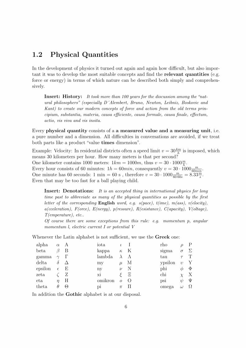
Whenever the Latin alphabet is not sufficient, we use the Greek one:

alpha α Abeta β Bgamma γ Γdelta δ ∆epsilon ε Ezeta ζ Zeta η Htheta θ Θ

iota ι Ikappa κ Klambda λ Λmy µ Mny ν Nxi ξ Ξomikron o Opi π Π

rho ρ Psigma σ Σtau τ Typsilon υ Yphi φ Φchi χ Xpsi ψ Ψomega ω Ω

In addition the Gothic alphabet is at our disposal.

6

1.3 Units

The units are defined in terms of yardsticks. The search for suitable yardsticks and theirdefinition, by as international a convention as possible, is an important part of science.

Insert: Standard units: What can be used as a standard unit? - The an-swers to this question have changed greatly through the centuries. Originally peopleeverywhere used easily available comparative quantities like cubit or foot as units oflength, and the human pulse beat as unit of time. (The Latin word tempora initiallymeant temple!) But not every foot has equal length, and the pulse can beat morequickly or slowly. Alone in Germany there have been more than 100 different cubitand foot units in use.

Therefore, since 1795 people referred to the ten millionth part of the earth meridianquadrant as the “meter” and represented this length by the well-known rod made outof an alloy of platinum and iridium. The measurement of time was referred to theearth’s rotation: for a long time the second was defined as the 86400th part of anaverage solar day.

In the meantime more exact atomic standards have been introduced: One meter is

now the distance light travels within the 1/299 792 485 part of a second. One second

is now defined in terms of the period of a certain oscillation of cesium 133 atoms in

“atomic clocks”. Perhaps some day these standards will also be improved.

Today, these questions are solved after many error ways by the conventions of the SI-units(Systeme International d’Unites) The following fundamental quantities are specified:

length measured in meters: mtime in seconds: smass in kilograms: kgelectric current in ampere: Atemperature in kelvin: Kluminous intensity in candelas: cdeven angle in radiant: radsolid angle in steradiant: sramount of material in mol: mol

All remaining physical quantities are to be regarded as derived, thus by laws, definitionsor measuring regulations traced back to the fundamental quantities: e.g.

7

frequency measured in hertz: Hz := 1/sforce in newton: N := kg m/s2

energy in joule: J := Nmpower in watt: W := J/spressure in pascal: Pa := N/m2

electric charge in coulomb: C := Aselectric potential in volt: V := J/Celectric resistance in ohm: Ω := V/Acapacitance in farad: F := C/Vmagnetic flux in weber: Wb := Vs

Exercise 1.1 SI-units

a) What is the SI-unit of momentum?

b) From which law can we deduce the unit of force?

c) Who formulated this law first?

d) What is the dimension of work?

e) What is the unit of the electric field strength?

Insert: Old units: Some examples of units which are still widely in use in spiteof the SI-convention:

grad: = (π/180)rad = 0.01745 radkilometer per hour: km/h = 0.277 m/shorse-power: PS = 735.499 Wcalorie: cal ' 4.185 Jkilowatt-hour: kWh = 3.6 · 106Jelektron volt: eV ' 1.6 · 10−19J

Many non-metric units are still used especially in England and the USA:

inch = Zoll: in = ” = 2.54 cmfoot: ft = 12 in ' 0.30 myard: yd = 3 ft ' 0.9144 m(amer.) mile: mil = 1760 yd ' 1609 mounce: oz ' 28.35 g(engl.) pound: lb = 16 oz ' 0.454 kg(amer.) gallon: gal ' 3.785 l(amer.) barrel: bbl = 42 gal ' 158.984 l

8

Exercise 1.2 Conversion of units

a) You are familiar with the conversion of angles from degrees to radiants using yourpocket calculator: Calculate 30, 45, 60, and 180 in radiant and 1 rad and 2 rad indegrees.

b) How many seconds make up one sidereal year with 12 months, 5 days, 6 hours, 9minutes and 9.5 seconds?

c) How much does it cost with an “electricity tariff” of 0.112 ¿/kWh, if you burn one nightlong a 60-Watt bulb for six hours and your PC runs needing approximately 200 watts?

d) Maria and Lucas measure their training distance with a stick, which is 5 feet and 2inches long. The stick fits in 254 times. What is the run called in Europe?How many rounds do Maria and Lucas have to run, until they put a mile back?

e) Bill Gates said: “If General Motors had kept up with technology like the computerindustry has, we would all be driving twenty-five dollar cars that go 1000 miles per gallon.”Did he mean the “3-litre car”?

1.4 Order of Magnitude

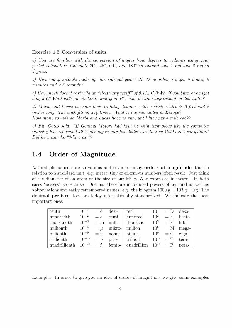
Natural phenomena are so various and cover so many orders of magnitude, that inrelation to a standard unit, e.g. meter, tiny or enormous numbers often result. Just thinkof the diameter of an atom or the size of our Milky Way expressed in meters. In bothcases “useless” zeros arise. One has therefore introduced powers of ten and as well asabbreviations and easily remembered names: e.g. the kilogram 1000 g = 103 g = kg. Thedecimal prefixes, too, are today internationally standardized. We indicate the mostimportant ones:

tenth 10−1 = d dezi- ten 101 = D deka-hundredth 10−2 = c centi- hundred 102 = h hecto-thousandth 10−3 = m milli- thousand 103 = k kilo-millionth 10−6 = µ mikro- million 106 = M mega-billionth 10−9 = n nano- billion 109 = G giga-trillionth 10−12 = p pico- trillion 1012 = T tera-quadrillionth 10−15 = f femto- quadrillion 1015 = P peta-

Examples: In order to give you an idea of orders of magnitude, we give some examples

9

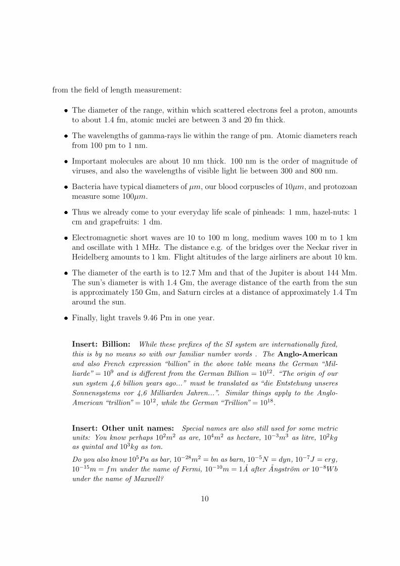
from the field of length measurement:

The diameter of the range, within which scattered electrons feel a proton, amountsto about 1.4 fm, atomic nuclei are between 3 and 20 fm thick.

The wavelengths of gamma-rays lie within the range of pm. Atomic diameters reachfrom 100 pm to 1 nm.

Important molecules are about 10 nm thick. 100 nm is the order of magnitude ofviruses, and also the wavelengths of visible light lie between 300 and 800 nm.

Bacteria have typical diameters of µm, our blood corpuscles of 10µm, and protozoanmeasure some 100µm.

Thus we already come to your everyday life scale of pinheads: 1 mm, hazel-nuts: 1cm and grapefruits: 1 dm.

Electromagnetic short waves are 10 to 100 m long, medium waves 100 m to 1 kmand oscillate with 1 MHz. The distance e.g. of the bridges over the Neckar river inHeidelberg amounts to 1 km. Flight altitudes of the large airliners are about 10 km.

The diameter of the earth is to 12.7 Mm and that of the Jupiter is about 144 Mm.The sun’s diameter is with 1.4 Gm, the average distance of the earth from the sunis approximately 150 Gm, and Saturn circles at a distance of approximately 1.4 Tmaround the sun.

Finally, light travels 9.46 Pm in one year.

Insert: Billion: While these prefixes of the SI system are internationally fixed,

this is by no means so with our familiar number words . The Anglo-American

and also French expression “billion” in the above table means the German “Mil-

liarde” = 109 and is different from the German Billion = 1012. “The origin of our

sun system 4,6 billion years ago...” must be translated as “die Entstehung unseres

Sonnensystems vor 4,6 Milliarden Jahren...”. Similar things apply to the Anglo-

American “trillion” = 1012, while the German “Trillion” = 1018.

Insert: Other unit names: Special names are also still used for some metricunits: You know perhaps 102m2 as are, 104m2 as hectare, 10−3m3 as litre, 102kgas quintal and 103kg as ton.

Do you also know 105Pa as bar, 10−28m2 = bn as barn, 10−5N = dyn, 10−7J = erg,

10−15m = fm under the name of Fermi, 10−10m = 1A after Angstrom or 10−8Wb

under the name of Maxwell?

10

Exercise 1.3 Decimal prefixes

a) Express the length of a stellar year (365 d + 6 h + 9 min + 9.5 s) in megaseconds.

b) The ideal duration of a scientific seminar talk amounts to one microcentury.

c) How long does a photon need, in order to fly with the speed of lightc = 2.997 924 58 ·108 m/s 21 m far through the lecture-room?

d) With the Planck energy of Ep = 1.22 · 1016 TeV gravitation effects for the elementaryparticles are expected. Express the appropriate Planck mass MP in grams.

In the following we are only concerned with the numerical values of the examinedphysical quantities, which we read off usually in the form of lengths or angles from ourmeasuring apparatuses, these being calibrated for the desired measuring range in appro-priate units of the measured quantities.

11

Chapter 2

SIGNS AND NUMBERSand Their Linkages

The laws of numbers and their linkages are the main objects of mathematics. Althoughnumbers have developed from basic needs of human social interaction, and natural sci-ence has inspired mathematics again and again, e.g. for differential and integral calculus,mathematics actually does not belong to natural sciences, but rather to humanities. Math-ematics does not start from empirical (i.e. measured) facts. Instead, it investigates thelogical structure of numbers and their generalizations within the human ability of thought.In many cases empirical facts can be well represented in terms of these logical structures.In this way mathematics became an indispensable tool for natural scientists and engineers.

2.1 Signs

Mathematics like every other science has developed its own language. This languageincludes among other things some mathematical and logical signs, which we would liketo list here for quick, clear reference, because we will be using them continually:

Question game: Some mathematical signs

The meaning of the following mathematical signs is known to most of you. ONLINE youcan challenge yourself and click directly on the symbols to check if you are right. If yourbrowser does not support this, you will find a complete list of answers here:

13

+: plus -: minus ± : plus or minus· : times /: divided by ⊥ : is perpendicular to<: is smaller than ≤: is smaller or equal to : is much smaller than=: is equal to 6=: is unequal to ≡: is identically equal to>: is bigger than ≥: is bigger or equal to : is much bigger than∠ : angle between ': is approximately equal to ∞ : bigger than every number

Insert: Infinity: Physicists often use the sign ∞, known as “infinity”, rather

casually. Assuming the meaning “bigger than every number” we avoid the problems

mathematicians warn us about: thus a < ∞ means a is a finite number. Shortly

we will use the combination of symbpols →∞ whenever we mean that a quantity is

“growing beyond all limits”.

In addition, we use the

Sum Sign∑

: for example3∑

n=1

an := a1 + a2 + a3

A famous example is the sum of the first m natural numbers:

m∑n=1

n := 1 + 2 + . . .+ (m− 1) +m =m

2(m+ 1),

just as the young Gauss has proved by skillful composition and clever use of brackets:m∑n=1

n = (1 +m) + (2 + (m− 1)) + (3 + (m− 2)) + . . . = m2

(m+ 1).

Another example is the sum of the first m squares of natural numbers:

m∑n=1

n2 := 1 + 4 + . . .+ (m− 1)2 +m2 =m

6(m+ 1)(2m+ 1),

a formula we will later need for the calculation of integrals.

A further example is the sum of the first m powers of a number q:

m∑n=0

qn := 1 + q + q2 + . . .+ qm−1 + qm =1− qm+1

1− qfor q 6= 1,

which is known as the “geometrical” sum.

14

Insert: Geometric sum: Just as an exception, we want to prove the formulafor the geometric series which we will need several times. To do this we define thesum

sm := 1+ q + q2 + . . .+ qm−1 + qm,

then we subtract from this q · sm = q + q2 + q3 + . . .+ qm + qm+1

and obtain (since nearly everything cancels)

sm − q · sm = sm(1− q) = 1− qm+1, from which we easily get for q 6= 1 dividing by

(1− q) the above formula for sm.

Much more important than the product sign∏

, defined analogously to the sum sign:

for instance3∏

n=1

an := a1 · a2 · a3 is for us the

factorial sign ! : m! := 1 · 2 · 3 · . . . · (m− 1) ·m =m∏n=1

n

(speak: “m factorial”), e.g. 3! = 1 ·2 ·3 = 6 or 5! = 120, augmented by the convention0! = 1.

Question game: Some logical signs

From the logical symbols which most of you are familiar with from math class, we use thefollowing symbols to display logical connections in a simpler, more concise, and memorableway, as well as to make it easier for us to memorize them. ONLINE you can click directlyon the symbols to get the answer. If your browser does not support this, you will find acomplete list of answers :

∈: is an element of 3: contains as element /∈: is no element of

⊆: is a subset of or equal ⊇: contains as a subset or is equal := : is defined by

∃: there exists ∃!: there exists exactly one ∀: for all

∪: union of sets ∩: intersection of sets ∅: empty set

⇒: from this it follows that, ⇐: this holds when, ⇔: this holds exactly when,is a sufficient condition for is a necessary condition for is a nec. and suff. cond. for

These symbols will be explained once more when they occur for the first time in the text.

15

2.2 Numbers

In order to display our measured data we need the numbers which you have been familiarwith for a long time. In order to get an overview, we shall put together here their propertiesas a reminder. In addition we recall some selected concepts which mathematicians haveformulated as rules for the combination of numbers, so that we can later on compare thoserules with the ones for more complicated mathematical quantities.

2.2.1 Natural Numbers

We begin with the set of natural numbers 1, 2, 3, . . ., given the name N by numbertheoreticians and called “natural” because they have been used by mankind to countwithin living memory. Physicists think for instance of particle numbers, e.g. the numberL of atoms or molecules in a mole.

Insert: Avogadro’s Number: Avogadro’s Number L is usually named after

Amedeo Avogadro (only in Germany after Joseph Loschmidt). It is a number with

24 digits from which only the first six ( 602213 ) are reliably known, while the next

two (67) are possibly affected by an error of (±36) Physicists use the following way

of writing: N = 6.022 136 7(36) · 1023.

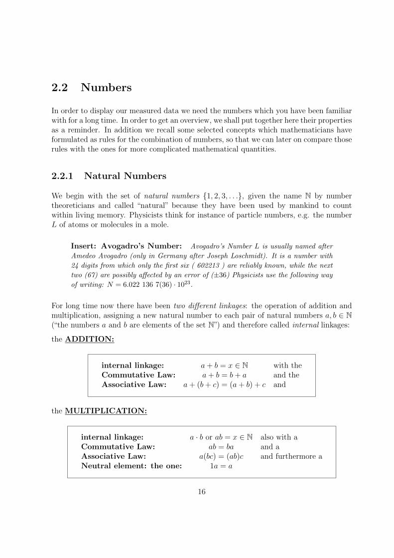
For long time now there have been two different linkages: the operation of addition andmultiplication, assigning a new natural number to each pair of natural numbers a, b ∈ N(“the numbers a and b are elements of the set N”) and therefore called internal linkages:

the ADDITION:

internal linkage: a+ b = x ∈ N with theCommutative Law: a+ b = b+ a and theAssociative Law: a+ (b+ c) = (a+ b) + c and

the MULTIPLICATION:

internal linkage: a · b or ab = x ∈ N also with aCommutative Law: ab = ba and aAssociative Law: a(bc) = (ab)c and furthermore aNeutral element: the one: 1a = a

16

Both linkages, addition and multiplication, are connected through the

Distributive Law: (a+ b)c = ac+ bc

with each other.

Insert: Shorthand: If we want to express that in the set of natural numbers

(n ∈ N) there exists only exactly one (∃!) element one which for all (∀) natural

numbers a fulfils the equation 1a = a , we could express this using the logical signs

in the following manner: ∃! 1 ∈ N : ∀a ∈ N 1a = a. Please appreciate this compact

logical writing.

Insert: Counter-examples: As an example of a linkage that leads out of a set,

we will soon deal with the well known scalar product of two vectors, which combines

their components into a simple number.

Non-communicative are for example the rotations of the match box shown in Figure

9.10 in a Cartesian coordinate system: First turn it clockwise around the longitu-

dinal symmetry axis parallel to the 3-axis and then around the shortest transversal

axis parallel to the 1-axis and compare the result with the position of the box after

you have performed the two rotations in the reversed order!

Counter-examples of the bracket law for three elements of a set are very hard to

find: From the home chemistry sector we remember the three ingredients for non-fat

whipped cream for children: ( sugar + egg-white ) + juice = cream. If you try to

whip first the egg-white together with juice as suggested by the instruction: sugar +

(egg-white + juice) you will never get the cream whipped.

We can clearly imagine the natural numbers as equally spaced points on a half line asshown in the next figure:

For physicists it is sometimes convenient to add the zero 0 as you would with a ruler, andso to extend N to N0 := N ∪ 0. Through this, the addition operation also obtains auniquely defined

17

Neutral element: the zero: 0 + a = a

In “logical shorthand”: ∃! 0 ∈ N0 : ∀a ∈ N0 : 0 + a = a in full analogy to the neutralelement of multiplication.

Insert: History: Even the ancient Greeks and Romans did not know numbers

other than the natural ones: N = I, II, III, IV, . . .. The Chinese knew zero as

“empty place” already in the 4th century BC. Not before the 12th century AD did

the Arabs bring the number zero to Europe.

2.2.2 Integers

Along with the progress in civilization and human culture it became necessary to extendthe numbers. For example, when talking about money it is not sufficient to know theamount (e.g. the number of coins) we also need to be able to express whether we have orowe that amount. Sometimes this is expressed through the colour of the number (“blackand red numbers”) or through a preceding + or − sign. In the natural sciences such signshave been established.

Physicists can shift a marking on their ruler by an arbitrary number of points to the right,they will however encounter difficulties if they want to move it to the left. Mathematicallyspeaking does not have for all natural numbers a and b the equation a+x = b a solution xwhich is itself a natural number: e.g. the equation 2+x = 1. Such equations can then onlybe solved if we extend the natural numbers through the negative numbers −a| a ∈ Nto form the set of all integers:

To every positive element a there exists exactly one

Negative element −a with: a+ (−a) = 0

Even for 1 we get a -1, meaning owing a pound in contrast to possessing a pound. In“logical shorthand” : ∀a ∈ Z ∃!− a : a+ (−a) = 0.

Mathematicians refer to the set of integers, which consist of all natural numbers a ∈ N,their negative partners −a ∈ (−N) and zero as Z := N ∪ 0 ∪ −a| a ∈ N.

With this extension, the above equation a+ x = b has now, as desired, always a solutionfor all pairs of integers, namely the difference x = b − a which once again is an integer

18

x ∈ Z. We also say that Z is “closed” concerning addition: i.e. addition does not lead outof the set. This brings us to a central concept in mathematics (and in physics), namelythat of a group :

We call a set of objects (e.g. the integers) a group, if

1. it is closed concerning an internal linkage (like e.g. addition),

2. an Associative Law holds (like e.g.: a+ (b+ c) = (a+ b) + c),

3. it encloses exactly one neutral element (like e.g. the number 0) and

4. if there exists exactly one reversal for each element (like e.g. the negative element).

If moreover the Commutative Law (like e.g. a+ b = b+ a) holds, mathematicians call thegroup Abelian.

Insert: Groups: Later on you will learn that groups play a very important role

in the search for symmetries in physics, e.g. for crystals or the classification of

elementary particles. The elements of a group are often operations, like e.g. rota-

tions: the result of two rotations performed one after the other can also be reached

by one single rotation. In performing three rotations the result does not depend on

the brackets. The operation no rotation leaves the body unchanged. Each rotation

can be cancelled. Usually these groups are not Abelian, e.g. two rotations performed

in different order yield different results. Therefore mathematicians did not incor-

porate the Commutative Law into the properties of groups. The more specialized

commutative groups are given the name Abelian after the Norwegian mathematician

Niels Henrik Abel (1802-1829).

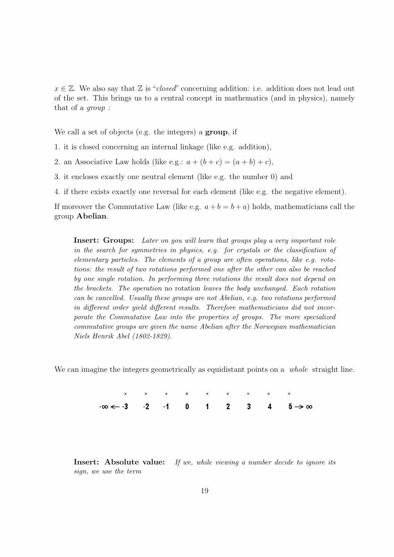
We can imagine the integers geometrically as equidistant points on a whole straight line.

Insert: Absolute value: If we, while viewing a number decide to ignore itssign, we use the term

19

absolute value: |a| := a for a ≥ 0 and |a| := −a for a < 0,

so that |a| ≥ 0 ∀a ∈ Z.For Instance for the number −5 : | − 5| = 5 and for the number 3 : |3| = 3 = 3.

The multiplication rule for the product of absolute values:

|a · b| = |a| · |b|

can easily be verified. For the absolute values of the sum and difference of integersthere hold only inequalities which we will meet later.

||a| − |b|| ≤ |a± b| ≤ |a|+ |b|.

The second part is known as “Triangle Inequality”.

The term |a− b| then gives the distance between the numbers a and b on the line of

numbers.

All points a in the neighbourhood interval of a point a0, having a distance from a0

which is smaller than a positive number ε is called a ε-neighbourhood Uε(a0) of a0 :

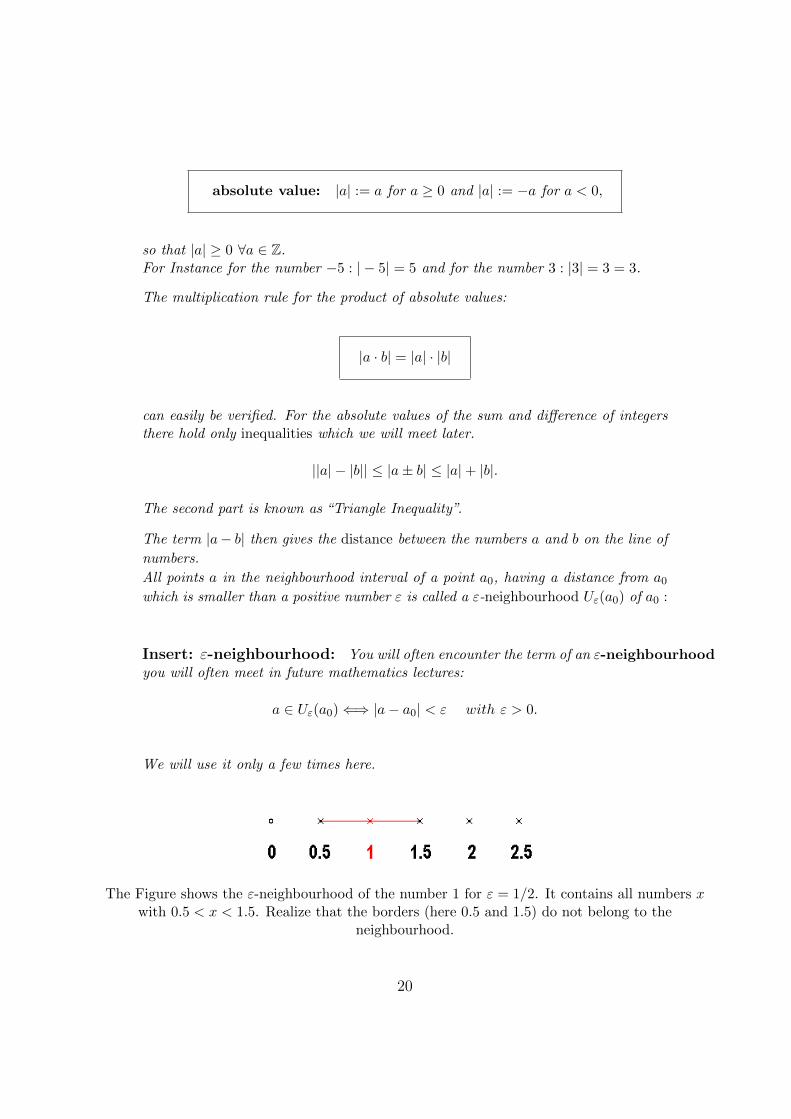
Insert: ε-neighbourhood: You will often encounter the term of an ε-neighbourhoodyou will often meet in future mathematics lectures:

a ∈ Uε(a0)⇐⇒ |a− a0| < ε with ε > 0.

We will use it only a few times here.

The Figure shows the ε-neighbourhood of the number 1 for ε = 1/2. It contains all numbers xwith 0.5 < x < 1.5. Realize that the borders (here 0.5 and 1.5) do not belong to the

neighbourhood.

20

2.2.3 Rational Numbers

Whenever people have been forced to do division, they have noticed that integers are notenough. Mathematically speaking: to solve the equation a · x = b for a 6= 0 within anumber set we are forced to extend the integers to rational numbers Q by adding theinverse numbers 1

aor a−1|a ∈ Z. We use the notation Z \ 0 for the set of integers

without the zero. Then we have for each integer a different from 0 exactly one

inverse element a−1 with: a · a−1 = 1

In “logical shorthand”: ∀a ∈ Z \ 0 ∃! a−1 : a · a−1 = 1.

We are familiar with this concept. The inverse to the number 3 is 13, the inverse number

to −7 is −17.

This way the fraction x = ba

for a 6= 0 solves our starting equation ax = b as desired. Ingeneral, a rational number is the quotient of two integers, consisting out of a numeratorand a denominator (different from 0). Rational numbers are therefore mathematicallyspeaking, ordered pairs of integers: x = (b, a).

Insert: Class: Strictly speaking one rational number is always represented by a

whole class of ordered pairs of integers, e.g. (1, 2) = (2, 4) = (3, 6) = (1a, 2a) for

a ∈ Q and a 6= 0 should be taken as one single number: 1/2 = 2/4 = 3/6 = 1a/2a :

Cancelling should not change the number, as we know.

When they are divided out, the rational numbers become finite, meaning breaking offor periodic decimal fractions: for example 1

5= 0.2 , 1

3= 0.3333333... = 0, 3 and 1

11=

0.09090909... = 0.09, where the line over the last digits indicates the period.

With this definition of the inverse elements the rational numbers form a group not onlyrelative to addition, but also, relative to multiplication (with the Associative Law, theone and the inverse elements). This group is, due to the Commutative Law of the factorsab = ba Abelian.

Insert: Field: For sets which form groups subject to two internal linkages

connected by a Distributive Law mathematicians have created a special name because

of their importance: They call such a set a field.

21

The rational numbers lie densely on our number line, meaning in every interval we canfind countable infinity of them:

Because of the finite accuracy of every physical measurement the rational numbers arein every practical aspect the working numbers of physics as well as in every othernatural science. This is why we had paid such an attention to their rules.

By stating results as rational numbers, mostly in the form of decimal fractions, scientistsworldwide have agreed on indicating only as many decimal digits as they have measured.Along with every measured value the uncertainty should also be indicated. This forexample is what we find in a table for Planck’s quantum of action

~ = 1.054 571 68(18) · 10−34 Js.

This statement can also be written in the following way:

~ = (1.054 571 68± 0.000 000 18) · 10−34 Js

meaning that the value of ~ (with a probability of 68 %) lies between the following twoborders:

1.054 571 50 · 10−34 Js ≤ ~ ≤ 1.054 571 86 · 10−34 Js.

Exercise 2.1

a) Show with the above indicated prescription of Gauss for even m, that the formula for

the sum of the first m natural numbersm∑n=1

n = m2

(m+ 1) holds also for odd m gilt.

b) Prove the above stated formula for the first m squares of natural numbersm∑n=1

n2 =

m6

(m+ 1)(2m+ 1) by consideringm∑n=1

(n+ 1)3

c) What do the following statements out of the “particle properties data booklet” mean:e = 1.602 176 53(14) · 10−19 Cb and me = 9.109 382 6(16) · 10−31 kg?

22

Insert: Powers: Repeated application of the same factor we describe usually aspower with the number of factors as

exponent: bn := b · b · b · · · b in case of n factors b,

where the known

calculation rules bnbm = bn+m, (bn)m = bn·m and (ab)n = anbn for n,m ∈ N

hold true. With the definitions b0 := 1 and b−n := 1/bn these calculation rules canbe extended to all integer exponents: n,m ∈ Z. Later we will generalize yet further.

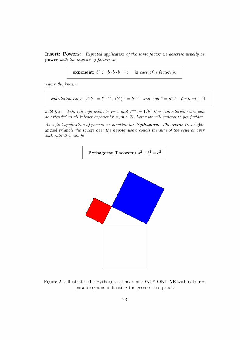
As a first application of powers we mention the Pythagoras Theorem: In a right-angled triangle the square over the hypotenuse c equals the sum of the squares overboth catheti a and b:

Pythagoras Theorem: a2 + b2 = c2

Figure 2.5 illustrates the Pythagoras Theorem, ONLY ONLINE with colouredparallelograms indicating the geometrical proof.

23

Very frequently we need the so-called

binomial formulas: (a± b)2 = a2 ± 2ab+ b2 and (a+ b)(a− b) = a2 − b2,

which can be easily derived, but need to be memorized.

The binomial formulas are a special case (for n = 2) of the more general formula

(a± b)n =n∑k=0

n!

k!(n− k)!an−k(±b)k,

where n!k!(n−k)!

=:(nk

)are the so-called binomial coefficients. We can calculate them

either directly from the definition of the factorial, e.g.(5

3

)=

5!

3!(5− 3)!=

1 · 2 · 3 · 4 · 51 · 2 · 3 · 1 · 2

= 10

or find them in the Pascal Triangle. This triangle is constructed in the following way:

n = 0 : 1n = 1 : 1 1n = 2 : 1 2 1n = 3 : 1 3 3 1n = 4 : 1 4 6 4 1n = 5 : 1 5 10 10 5 1n = 6 : 1 6 15 20 15 6 1

We start with the number 1 in the line n = 0. In the next line (n = 1) we write two ones,one on each side. Then for n = 2 we add two ones to the left and right side once again,and in the gap between them a 2 = 1 + 1 as the sum of the left and right “front man”(in each case a 1). In the framed box, we once again recognize the formation rule. Therequired binomial coefficient

(53

)is then found in line n = 5 on position 3.

Exercise 2.2

a) Determine the length of the space diagonal in a cube with side length a.

b) Calculate (a4 − b4)/(a− b).

c) Calculate(n0

)and

(nn

).

d) Calculate(

74

)and

(83

).

e) Show that(

nn−k

)=(nk

)holds true.

f) Prove the formation rule for the Pascal Triangle:(nk−1

)+(nk

)=(n+1k

).

24

2.2.4 Real Numbers

Mathematicians were however not fully satisfied with the rational numbers, seeing howfor example something as important as the circumference π of a circle with the diameterof 1 is not a rational number: π /∈ Q. They also wanted the solution of the equationx2 = a at least for a 6= 0, as well as the roots x = a1/2 =:

√a to be included. This is why

the rational numbers (by addition of infinite decimal fractions) have been extended to thereal numbers R which can be mapped one-to-one onto a straight line R1 (meaning everypoint on the line corresponds to exactly one real number).

Insert: History: Already in antiquity some mathematicians knew that there arenumbers which cannot be represented as fractions. They showed this with a so-calledindirect proof:

If e.g. the diagonal of a square with side length 1 were a rational number, like√2 = b/a, two natural numbers b, a ∈ N would exist with b2 = 2a2. Think now of

the prime factor decompositions of b and a. On the left hand side of the equationthere stands an even number of these factors, because of the square each factorappears twice. On the right hand side, however, an odd number of factors shows up,because in addition the factor 2 appears. Since the prime factor decomposition isunique, the equation cannot be right.

With this it is shown that the assumption,√

2 can be represented as a fraction, leads

to a contradiction and thus must be wrong.

With the real numbers, which have the same calculation rules of a field as the rationalnumbers, both solutions of the general

quadratic equation: x2 + ax+ b = 0, x1,2 = −a2±√a2

4− b

will then be real numbers, as long as the discriminant under the root is not negative:a2 ≥ 4b.

Insert: Preview: complex numbers: Later in Chapter 8 we will go one

step further by introducing the complex numbers C for which e.g. also x2 = a

for a < 0 is always solvable and, amazingly enough, many other beautiful laws hold.

25

Chapter 3

SEQUENCES AND SERIESand Their Limits

Direct mathematical study of sequences and series are, for natural scientists, less im-portant than the fact that they greatly help us to understand and perform the limitingprocedures which are of fundamental importance in physics. For this reason, we havecombined in this chapter the most important facts of this part of mathematics. Later youwill deal in greater detail with these things in your future mathematics lectures.

3.1 Sequences

The first important mathematical concept we have to inspect is that of a sequence.With this physicists think for instance of the sequence of the bounce heights of a steelball on a plate, which due to the inevitable dissipation of energy decrease with time andtend more or less quickly to zero. After a while, the ball remains still. The resultingphysical sequence of the jump heights has only a finite number of non-vanishing membersin contrast to the ones that are of interest to mathematicians: Mathematically, a sequenceis an infinite set of numbers which can be numbered consecutively, i.e. labelled by theset of the natural numbers: (an)n∈N. Because it is impossible to list all infinite manymembers (a1, a2, a3, a4, a5, a6, . . .), a sequence is mostly defined by the “general member”an, which is a law stating how to calculate the individual members of the sequence. Letus look at the following typical examples which already enable us to display all importantconcepts:

27

(F1) 1, 2, 3, 4, 5, 6, 7, . . . = (n)n∈N the natural numbers themselves(F2) 1,−1, 1,−1, 1,−1, . . . = ((−1)n+1)n∈N a simple “alternating” sequence,(F3) 1, 1

2, 1

3, 1

4, 1

5, . . . =

(1n

)n∈N the inverse natural numbers,

the so-called “harmonic” sequence,(F4) 1, 1

2, 1

6, 1

24, . . . =

(1n!

)n∈N the inverse factorials,

(F5) 12, 2

3, 3

4, 4

5, . . . =

(nn+1

)n∈N

a sequence of proper fractions and

(F6) q, q2, q3, q4, q5 . . . = (qn)n∈N , q ∈ R the “geometric” sequence.

Insert: Compound interest: Many of you know the geometrical sequence

from school because it causes a capital K0 at p% compound interest after n years to

increase to Kn = K0qn with q = 1 + p

100 .

In order to give us a first clear idea of these sample sequences, we have plotted thesequence members an (in the 2-direction) over the equidistant natural numbers n (in the1-direction) in the following Cartesian coordinate system in a plane:

Figure 3.1: Visualization of our sample sequences over the natural numbers, in case of thegeometrical sequence (F6) for q = 2 and q = 1

2.

Also the sum, the difference or the product of two sequences are again a sequence. Forexample, the sample sequence (F5) with an = n

n+1= n+1−1

n+1= 1 − 1

n+1is the difference

of the trivial sequence (1)n∈N = 1, 1, 1, . . ., consisting purely of ones, and the harmonicsequence (F3) except for the first member.

The termwise product of the sample sequences (F2) and (F3) makes up a new sequence:

(F7) 1,−12, 1

3,−1

4, ... =

((−1)n+1

n

)n∈N

the “alternating” harmonic sequence.

Similarly the termwise product of the harmonic sequence (F3) with itself is once again asequence:

28

(F8) 1, 14, 1

9, 1

16, ... =

(1n2

)n∈N the sequence of the inverse natural squares.

The termwise product of the sample sequences (F1) and (F6), too, gives a new sequence:(F9) q, 2q2, 3q3, 4q4, 5q5 . . . = (nqn)n∈N, q ∈ R a modified geometric sequence.

An other more complicated combined sequence will attract our attention later:

(F10) 2, (32)2, (4

3)3, . . . =

((1 + 1

n)n)n∈N the so-called exponential sequence.

Exercise 3.1 Illustrate these additional sample sequences graphically. Project thepoints on the 2-axis.

There are three characteristics that are of special interest to us as far as sequences areconcerned: boundedness, monotony and convergence:

3.2 Boundedness

A sequence is called bounded above, if there is an upper bound B for the members ofthe sequence: an ≤ B: in shorthand notation this means:

(an)n∈N bounded above ⇐⇒ ∃B : an ≤ B ∀n ∈ N

Bounded below is defined in full analogy with a lower lower bound A:∃A : A ≤ an ∀n ∈ N.

For example, our first sample sequence (F1) consisting of the natural numbers is boundedonly from below e.g. by 1: A = 1. The alternating sequence (F2) is obviously boundedfrom above and from below, e.g. by A = −1 and B = 1, respectively. For the harmonicsequence (F3) the first member, the 1, is an upper bound: B = 1 ≥ 1

n∀n ∈ N and the

zero a lower one: A = 0. The sample sequence (F4) of the inverse factorials has the lowerbound A = 0 and the upper one B = 1.

Exercise 3.2 Investigate the boundedness of the other two of our sample sequences.

29

3.3 Monotony

A sequence is said to be monotonically increasing, if the successive members increasewith increasing number: To memorize:

(an)n∈N monotonically increasing ⇐⇒ an ≤ an+1 ∀n ∈ N.

If the stronger condition an an+1 holds true, one calls the sequence strictly monotonicincreasing.

In full analogy, monotonically decreasing is defined with an ≥ an+1.

For example, the sequence (F1) of the natural numbers is strictly monotonic increasing,the alternating harmonic sequence (F2) is not monotonic at all and the harmonic sequence(F3) as well as the sequence (F4) of the inverse factorials are strictly monotonic decreasing.

Exercise 3.3 Monotonic sequences

Investigate the monotony of the other two of our sample sequences.

3.4 Convergence

Now we come to the central topic of the whole chapter: As you may have seen from theprojection of the visualizing points onto the 2-axis there are sequences, whose membersan accumulate around a number a on the number line, so that infinitely many membersof the sequence lie in every ε-neighbourhood Uε(a) of this number a, which by the wayneeds not necessarily to be itself a member of the sequence. We call a in such a case acluster point of the sequence.

In our examples we immediately realize that the sequence (F1) of the natural numbershas none and the harmonic sequence (F3) has one cluster point, namely the zero. Thealternating sequence (F2) has even two cluster points: one at +1 and one at −1.

The Theorem of Bolzano and Weierstrass guarantees, that every sequence which isbounded above and below has to have at least one cluster point.

In the case that a sequence has only one single cluster point, it may occur that all sequencemembers from a certain number on, lie in the neighbourhood of that point. We then callthis point the limit of the sequence and this situation turns out to be the central concept

30

of analysis: Therefore mathematicians have several terms for it: They also say that thesequence converges or is convergent to a and write: lim

n→∞an = a, or sometimes more

casually: ann→∞−→ a.

(an)n∈N convergent: ∃a : limn→∞

an = a

⇐⇒ ∀ε > 0 ∃N(ε) ∈ N : |an − a| < ε ∀n > N(ε).

The last shorthand reads: for every pre-set positive number ε which may be as tiny asyou like, you can find a number N(ε) so that the distance from the cluster point a for allsequence members with a number larger than N(ε) is smaller than the pre-given small ε.

For many sequences we can recognize the convergence or even the limit value with someskill just by looking at it. But sometimes it is by no means easy to determine whethera sequence is convergent. This is why the Theorem of Bolzano and Weierstrass is somuch appreciated: It shows us very generally when we can conclude the convergence of asequence:

Theorem of Bolzano and Weierstrass:Every monotonically increasing sequence which is bounded above isconvergent, andevery monotonically decreasing sequence which is bounded below isconvergent, respectively.

In all cases where the limiting value is unknown or not easily identifiable mathematiciansoften make also use of the necessary (⇐) and sufficient (⇒)

Cauchy-Criterion: (an) convergent⇐⇒ ∀ε > 0 ∃N(ε) ∈ N : |an − am| < ε ∀n,m > N(ε)

meaning, a sequence converges if and only if from a certain point onward the distancesbetween the members of the sequence decrease more and more, i.e. the correspondingpoints on the number axis move closer and closer together. If that is not the case thesequence diverges. In addition, it can be shown that every subsequence of a convergentsequence and the sum and difference as well as the product and (provided the denominator

31

is different from zero) also the quotient of two convergent sequences are convergent as well.This means that the limit is commutable with the rational arithmetic operations.

Many convergent sequences tend to zero as their cluster point, we call them zero sequences.

The harmonic sequence (F3) with an = 1n

is for example such a zero sequence.

Insert: Convergence proofs: For the sequence F3:( 1n)n∈N we want to test

all convergence criteria:

1. Most easily we check the Theorem of Bolzano and Weierstrass: the sequence(F3)( 1

n)n∈N is monotonically decreasing and bounded below: 0 < 1n , consequently it

converges.

2. The cluster point is apparently a = 0 : We pre-set an ε > 0 arbitrarily, e.g.ε = 1

1000 and look for a number N(ε), so that |an − a| = | 1n − 0| = | 1n | =1n < ε for

n > N(ε). That is surely the case if we choose N(ε) as the next natural numberlarger than 1

ε : N(ε) > 1ε (e.g. for ε = 0.001 we take N(ε) = 1001). Then there

holds for all n > N(ε) : 1n <

1N(ε) < ε.

3. Finally also the Cauchy Criterion can easily be checked here: If a certain ε > 0

is pre-given, it follows for the distance of two members an and am with n < m :

|an − am| = | 1n −1m | = |

m−nnm | < |

mnm | =

1n < ε, if n > N(ε) = 1

ε .

The sequences (F1) and (F2) obviously do not converge.

Exercise 3.4 Convergent sequences

a) Test the other three sample sequences for convergence.

b) Calculate - in order to become cautious - the first ten members of the sequence an =n · 0.9n, the product of (F1) with (F6) for q = 0.9, and compare with a60, as well as ofan = n!

10n, the quotient of (F6) for q = 1

10and (F4), and compare with the corresponding

a60.

c) The sequence consisting alternately of the members of (F1) and (F3): i.e. 1,12,3,1

4,5,1

6,. . .

has only one single cluster point, namely 0. Does it converge to 0?

3.5 Series

After having studied the limits of number sequences, we can apply our newly acquiredknowledge to topics which occur more often in physics, for instance infinite sums s =∞∑n=1

an, called series:

32

These are often encountered sometimes in more interesting physical questions: For in-stance if we want to sum up the electrostatic energy of infinitely many equidistant alter-nating positive and negative point charges for one chain link (which gives a simple butsurprisingly good one-dimensional model of a ion crystal) we come across the infinite sum

over the members of the alternating harmonic sequence (F7): the series∞∑n=1

(−1)n+1

n. How

do we calculate this?

Series are sequences whose members are finite sums of real numbers: The definition of a

series∞∑

n=1

an as sequence of partial sums sm =

(m∑n=1

an

)m∈N

reduces the series to sequences which we have been dealing with just above.

Especially, a series is exactly then convergent and has the value s, if the sequence of itspartial sums sm (not that of its summands an!!) converges: lim

m→∞sm = s:

series sm =m∑n=1

an convergent ⇐⇒ limm→∞

m∑n=1

an = s <∞

Also the multiple of a convergent series and the sum and difference of two convergentseries are again convergent.

The few sample series that we need, to see the most important concepts, we derive simplythrough piecewise summing up our sample sequences:

(R1) The series of the partial sums of the sequence (F1) of the natural numbers:

sm =

(m∑n=1

n

)m∈N

= 1, 3, 6, 10, 15, . . . is clearly divergent.

(R2) The series made out of the members of the alternating sequence (F2) always jumpsbetween 1 and 0 and has therefore two cluster points and consequently no limit.

(R3) Also the“harmonic series” summed up out of the members of the harmonic sequence

(F3), i.e. the sequence

(sm =

m∑n=1

1n

)m∈N

= 1, 32, 11

6, 25

12, 137

60, . . . is divergent. Because the

(also necessary) Cauchy Criterion is not fulfilled: If we for instance choose ε = 14> 0 and

consider a piece of the sequence for n = 2m consisting of m terms: |s2m−sm| =2m∑

n=m+1

1n

=

33

1m+1

+ 1m+2

+ . . . + 12m

>1

2m+

1

2m+ . . .+

1

2m︸︷︷︸m summands

= 12> ε = 1

4while for convergence < ε

would have been necessary.

(R7) Their alternating variant however, created out of the sequence (F7), our physical

example from above, converges∞∑n=1

(−1)n+1

n(= ln 2, as we will show later).

Because of this difference between series with purely positive summands and alternatingones, it is appropriate to introduce a new term: A series is said to be absolutely convergent,if already the series of the absolute values converges.

Series sm =m∑n=1

an absolutely convergent ⇐⇒ limm→∞

m∑n=1

|an| <∞

We can easily understand that within an absolutely convergent series the summands canbe rearranged without any effect on the limiting value. Two absolutely convergent seriescan be multiplied termwise to create a new absolutely convergent series.

For absolute convergence the mathematicians have developed various sufficient criteria,the so-called majorant criteria which you will deal with more closely in the lecture aboutanalysis:

Insert: Majorants: If a convergent majorant sequence S = limm→∞

Sm =∞∑n=1

Mn

exists with positive Mn > 0, whose members are larger than the correspondingabsolute values of the sequence under examination Mn ≥ |an|, then the series

limm→∞

sm =∞∑n=1

an is absolutely convergent, because from the Triangle Inequality

it follows

|sm| = |m∑n=1

an| ≤m∑n=1|an| ≤

m∑n=1

Mn = Sm.

Very often the “geometric series”

(R6):∞∑n=0

qn, which follow from the geometric sequences (F6) (qn)n∈N, q ∈ R , serve as

majorants. To calculate them we benefit from the earlier for q 6= 1 derived geometric sum:

limm→∞

m∑n=0

qn = limm→∞

1− qm+1

1− q=

1

1− q<∞,

meaning convergent for |q| < 1 and divergent for |q| ≥ 1.

34

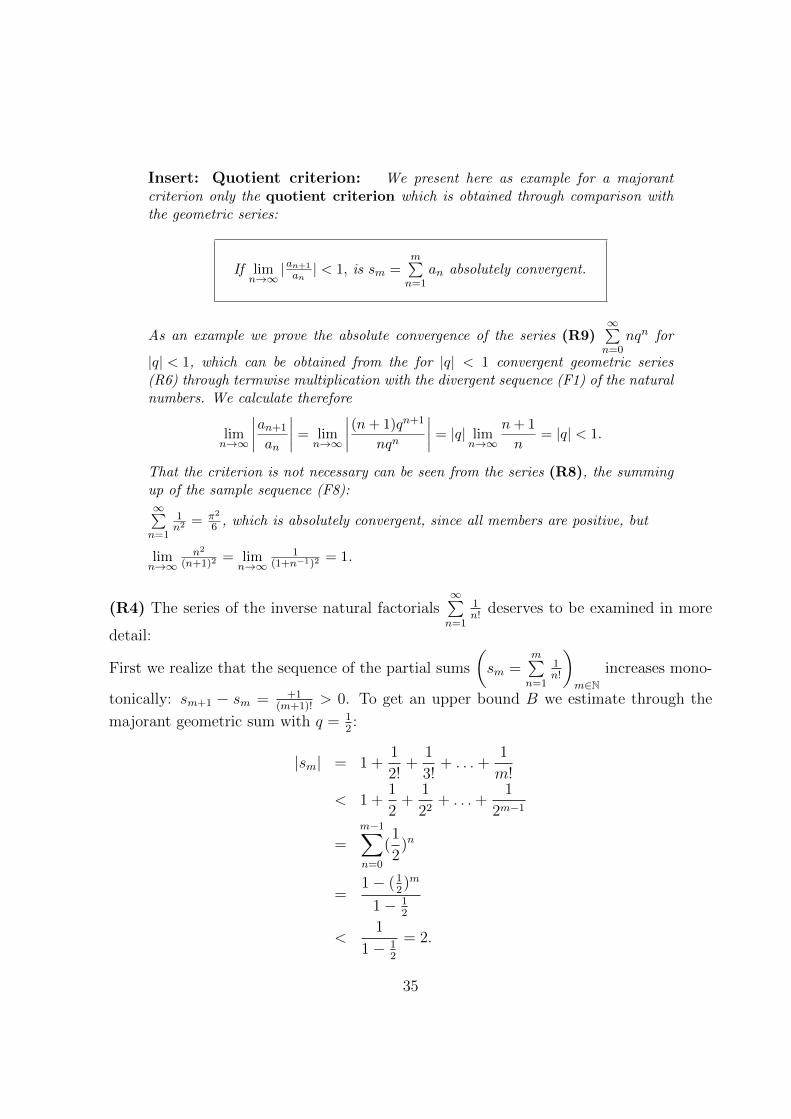
Insert: Quotient criterion: We present here as example for a majorantcriterion only the quotient criterion which is obtained through comparison withthe geometric series:

If limn→∞

|an+1

an| < 1, is sm =

m∑n=1

an absolutely convergent.

As an example we prove the absolute convergence of the series (R9)∞∑n=0

nqn for

|q| < 1, which can be obtained from the for |q| < 1 convergent geometric series(R6) through termwise multiplication with the divergent sequence (F1) of the naturalnumbers. We calculate therefore

limn→∞

∣∣∣∣an+1

an

∣∣∣∣ = limn→∞

∣∣∣∣(n+ 1)qn+1

nqn

∣∣∣∣ = |q| limn→∞

n+ 1

n= |q| < 1.

That the criterion is not necessary can be seen from the series (R8), the summingup of the sample sequence (F8):∞∑n=1

1n2 = π2

6 , which is absolutely convergent, since all members are positive, but

limn→∞

n2

(n+1)2= lim

n→∞1

(1+n−1)2= 1.

(R4) The series of the inverse natural factorials∞∑n=1

1n!

deserves to be examined in more

detail:

First we realize that the sequence of the partial sums

(sm =

m∑n=1

1n!

)m∈N

increases mono-

tonically: sm+1 − sm = +1(m+1)!

> 0. To get an upper bound B we estimate through the

majorant geometric sum with q = 12:

|sm| = 1 +1

2!+

1

3!+ . . .+

1

m!

< 1 +1

2+

1

22+ . . .+

1

2m−1

=m−1∑n=0

(1

2)n

=1− (1

2)m

1− 12

<1

1− 12

= 2.

35

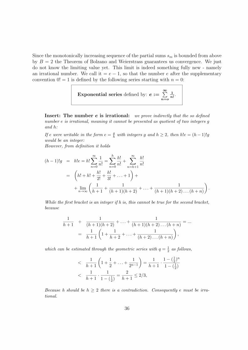
Since the monotonically increasing sequence of the partial sums sm is bounded from aboveby B = 2 the Theorem of Bolzano and Weierstrass guarantees us convergence. We justdo not know the limiting value yet. This limit is indeed something fully new - namelyan irrational number. We call it = e − 1, so that the number e after the supplementaryconvention 0! = 1 is defined by the following series starting with n = 0:

Exponential series defined by: e :=∞∑

n=o

1n!

.

Insert: The number e is irrational: we prove indirectly that the so definednumber e is irrational, meaning it cannot be presented as quotient of two integers gand h:

If e were writable in the form e = gh with integers g and h ≥ 2, then h!e = (h− 1)!g

would be an integer:However, from definition it holds

(h− 1)!g = h!e = h!∞∑n=0

1

n!=

h∑n=0

h!

n!+

∞∑n=h+1

h!

n!

=

(h! + h! +

h!

2!+h!

3!+ . . .+ 1

)+

+ limn→∞

(1

h+ 1+

1

(h+ 1)(h+ 2)+ . . .+

1

(h+ 1)(h+ 2) . . . (h+ n)

).

While the first bracket is an integer if h is, this cannot be true for the second bracket,because

1

h+ 1+

1

(h+ 1)(h+ 2)+ . . .+

1

(h+ 1)(h+ 2) . . . (h+ n)= ...

=1

h+ 1

(1 +

1

h+ 2+ . . .+

1

(h+ 2) . . . (h+ n)

),

which can be estimated through the geometric series with q = 12 as follows,

<1

h+ 1

(1 +

1

2+ . . .+

1

2n−1

)=

1

h+ 1·

1− (12)n

1− (12)

<1

h+ 1· 1

1− (12)

=2

h+ 1≤ 2/3,

Because h should be h ≥ 2 there is a contradiction. Consequently e must be irra-

tional.

36

To get the numerical value of e we first calculate the members of the zero sequence(F4) an = 1

n!:

a1 = 11!

= 1, a2 = 12!

= 12

= 0.50, a3 = 13!

= 16

= 0.1666,a4 = 1

4!= 1

24= 0.041 666, a5 = 1

5!= 1

120= 0.008 33,

a6 = 16!

= 1720

= 0.001 388, a7 = 17!

= 15 040

= 0.000 198,a8 = 1

8!= 1

40 320= 0.000 024, a9 = 1

9!= 1

362 880= 0.000 002, . . .

then we sum up the partial sums: sm =m∑n=1

1n!

= 1 + 12!

+ 13!

+ 14!

+ . . .+ 1m!

s1 = 1, s2 = 1.50, s3 = 1.666 666, s4 = 1.708 333,s5 = 1.716 666, s6 = 1.718 055, s7 = 1.718 253,s8 = 1.718 278, s9 = 1.718 281, . . ..

If we look at the rapid convergence, we can easily imagine that after a short calculationwe receive the following result for the limiting value: e = 2.718 281 828 459 045 . . .

Insert: A sequence converging to e: Besides this exponential series whichwe used to define e there exists as earlier mentioned in addition a sequence, con-verging to the number e, the exponential sequence(F10):((1 + 1

n)n)n∈N = 2, (3

2)2, (43)3, . . . , which we will shortly deal with for comparison:

According to the binomial formula we find firstly for the general sequence member:

an = (1 +1

n)n =

n∑k=0

n!

(n− k)!k!nk

= 1 +n

n+n(n− 1)

n22!+n(n− 1)(n− 2)

n33!+ . . .+

n(n− 1)(n− 2) . . . (n− (k − 1))

nkk!+

. . .+n!

nnn!

= 1 + 1 +(1− 1

n)

2!+

(1− 1n)(1− 2

n)

3!+ . . .+

(1− 1n)(1− 2

n) . . . (1− k−1n )

k!+ . . .

+(1− 1

n)(1− 2n) . . . (1− n−1

n )

n!

On the one hand we enlarge this expression for an, by forgetting the subtractionof the multiples of 1

n within the brackets:

an ≤ 1 + 1 +1

2!+

1

3!+ . . .+

1

n!= 1 + sn

and reach so (besides the term one) the corresponding partial sums of the exponentialseries sn. Thus the exponential series is a majorant for the also monotonicallyincreasing exponential sequence and ensures the convergence of the sequence throughthat of the series. For the limiting value we get:

37

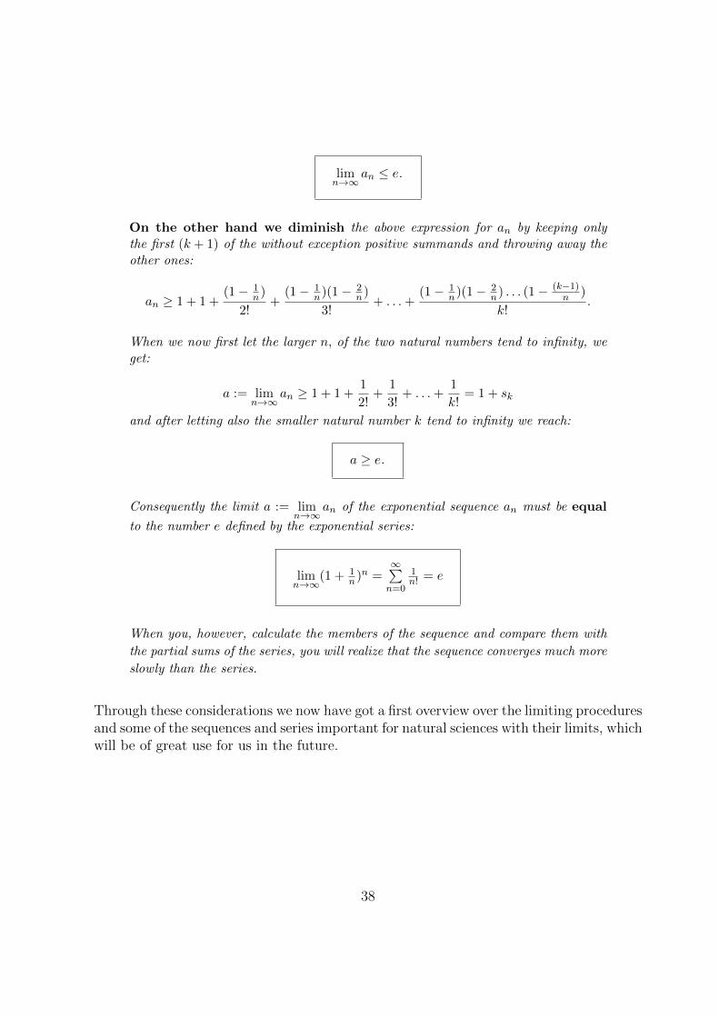
limn→∞

an ≤ e.

On the other hand we diminish the above expression for an by keeping onlythe first (k + 1) of the without exception positive summands and throwing away theother ones:

an ≥ 1 + 1 +(1− 1

n)

2!+

(1− 1n)(1− 2

n)

3!+ . . .+

(1− 1n)(1− 2

n) . . . (1− (k−1)n )

k!.

When we now first let the larger n, of the two natural numbers tend to infinity, weget:

a := limn→∞

an ≥ 1 + 1 +1

2!+

1

3!+ . . .+

1

k!= 1 + sk

and after letting also the smaller natural number k tend to infinity we reach:

a ≥ e.

Consequently the limit a := limn→∞

an of the exponential sequence an must be equal

to the number e defined by the exponential series:

limn→∞

(1 + 1n)n =

∞∑n=0

1n! = e

When you, however, calculate the members of the sequence and compare them with

the partial sums of the series, you will realize that the sequence converges much more

slowly than the series.

Through these considerations we now have got a first overview over the limiting proceduresand some of the sequences and series important for natural sciences with their limits, whichwill be of great use for us in the future.

38

Chapter 4

FUNCTIONS

4.1 The Function as Input-Output Relation or Map-

ping

We would like to remind you of the empirical method of physics discussed in Chapter 1,and take a look at the simplest, but common case: in an experiment we investigate themutual dependency of two physical quantities: “y as a function of x” or y = f(x): In ourexperiment one quantity x, called the independent variable, is measurably changed andthe second quantity y, the dependant variable, is measured in each case. We may imaginethe measuring apparatus in the way depicted below as a black box, into which the x arefed in as input, and from which the corresponding y come out as output.

Figure 4.1: Function as a black box with x as input and y as output

Physicists think for example of an electric circuit where the voltage is changed gradually bya potentiometer and the electric current is measured with a mirror galvanometer in orderto investigate the characteristic curve. Also the time development of the amplitude of apendulum or a radioactively decaying material as function of time are further candidatesout of the huge number of physical examples.

39

The result of such a series of measurements is first of all a value table (x, y). The data canalso be displayed in a graphic illustration, as shown below in our samples. Illustration ofthe functions as a picture, usually called by us graph, through plotting the measured valuesin a plane with a Cartesian (meaning right-angled) coordinate system (with the abscissax on the 1-axis and the ordinate y on the 2-axis) is a matter of course for physicists.

In the following figures you will find examples for value tables, graphic illustrations andinterpolating functions for a swinging spiral spring

xcm

FmN

1 −0.421.5 −0.552 −0.822.5 −1.033 −1.253.5 −1.454 −1.654.5 −1.805 −1.955.5 −2.206 −2.356.6 −2.60

Figure 4.2 a: Reaction force F of the spring measured in mN in dependency on theamplitude x in cm.

xcm

EmJ

1 0.6

1.5 1.0

2.5 2.8

2.9 3.9

3.1 4.8

3.5 6.1

Figure 4.2 b: Potential energy E stored in the spring measured in mJ in dependency onthe amplitude x in cm.

40

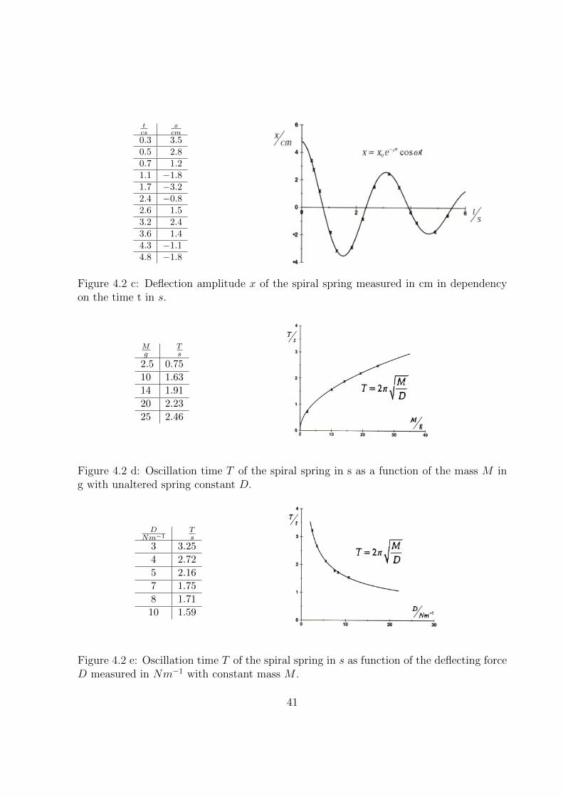
tcs

xcm

0.3 3.50.5 2.80.7 1.21.1 −1.81.7 −3.22.4 −0.82.6 1.53.2 2.43.6 1.44.3 −1.14.8 −1.8

Figure 4.2 c: Deflection amplitude x of the spiral spring measured in cm in dependencyon the time t in s.

Mg

Ts

2.5 0.75

10 1.63

14 1.91

20 2.23

25 2.46

Figure 4.2 d: Oscillation time T of the spiral spring in s as a function of the mass M ing with unaltered spring constant D.

DNm−1

Ts

3 3.25

4 2.72

5 2.16

7 1.75

8 1.71

10 1.59

Figure 4.2 e: Oscillation time T of the spiral spring in s as function of the deflecting forceD measured in Nm−1 with constant mass M .

41

After we have taken into account the inevitable measurement errors, we can start con-necting the measured points by a curve or a mathematical calculation instruction, to lookfor a function which describes the dependence of the two quantities. If we succeed infinding such a function, we have achieved real progress: A mathematical formula is usu-ally short and concise; it can be stapled, processed and conveyed to others much easierthan extensive value tables. With its help we are able to interpolate more closely betweenthe measurements and to extrapolate beyond the measured area, which suggests furtherexperiments. Finally it is the first step towards a theory, and with it to the understandingof the experiment.

Insert: History: T. Brahe measured in his laboratory the position of the planet

Mars at different times. From that value table J. Kepler found the ellipse as an

interpolating function for the orbit curve. This result influenced I. Newton in finding

his gravitation law.

Therefore, for physical reasons, we have to deal with functions, first with real functionsof a real variable.

Mathematically, we can consider a function y = f(x) as an unambiguous mapping x →f(x) of a point x of the area Df , (the “definition domain” of f) of the independentvariable x (also known as abscissa or argument) onto a point f(x) of the area Wf (the“value domain” of f) of the dependent variable y (also known as ordinate or functionvalue).

While the declaration of the definition domain in addition to the mapping prescriptionis absolutely necessary for a function, and often influences the properties of the function,the exact statement of the value domain Wf := f(x)|x ∈ Df is in most cases of lessimportance and sometimes takes much effort.

Figure 4.3: Function f as a mapping of the definition domain Df into the value domainWf (with two arrows, which lead from two pre-image points to one image point)

42

The pre-image set Df is in most cases, just as is the set of images Wf , a part of the realnumber axis R1. The unambiguity included in the definition of a real function means thatto each x there is one and only one y = f(x). (It is however possible that two differentpre-image points are mapped into one and the same image point.) To summarize inmathematical shorthand:

y = f(x) function: ∀x ∈ Df ⊆ R1 ∃!y = f(x) : y ∈ Wf ⊆ R1

The arithmetic for real functions of a real variable follows according to the rules ofthe field R with both the Commutative and Associative Laws, as well as the connectingDistributive Law, which we have put together for the numbers in Chapter 2 : for example,the sum or the difference of two real functions f1(x)± f2(x) = (f1 ± f2)(x) =: g(x) givesa new real function, as well as the real multiple r · f(x) = (r · f)(x) =: g(x) with r ∈ Rand analogously also the product f1(x) · f2(x) = (f1 · f2)(x) =: g(x) or, if f2(x) 6= 0 all

over the definition domain, the quotient, too. f1(x)f2(x)

= f1f2

(x) =: g(x).

4.2 Basic Set of Functions

It is surprising that we can manage to go through daily physics with a basic set of veryfew functions which moreover you are mostly acquainted with from school. In this sectionwe will introduce these basic set of functions as examples, then discuss some of theircharacteristics, and come back to them again and again.

4.2.1 Rational Functions

We start with the constant function y = c, independent of x. Afterwards we come tolinear functions y = s · x+ c with the graph of a straight line having a gradient s and theordinate section c. We proceed to the standard parabola y = x2 and the higher powersy = xn with n ∈ N. Also the standard hyperbola y = 1

x= x−1 and y = 1

x2which you are

surely familiar with.

Straight line and parabola are for example defined over the whole real axis: Df = R. Forthe hyperbola we must omit the origin: Df = R \ 0. Also in the image domain of thehyperbola the origin is missing: Wf = R \ 0. For the parabola the image domain isonly the positive half-line including zero: y ≥ 0. The following figure shows the graphs ofthese simple examples:

43

Figure 4.4: Graphs of simple functions

According to the calculation rules of the field of real numbers R we get from the straightline and the standard parabola y = x2 all functions of second degree y = ax2 + bx+ c aswell as all further polynomial functions of higher, e.g. m−th degree:

y = Pm(x) = a0 + a1x+ a2x2 + . . .+ amx

m =m∑k=0

akxk.

Even the general rational function

y(x) = R(x) =Pm(x)

Qn(x)

with a polynomial of m−th degree Pm(x) in the numerator and a polynomial of the n−thdegree Qn(x) in the denominator you are surely familiar with, for example y = 1

x2+1,

the Lorentz distribution, which among other things describes the natural line width of aspectral line with D = R and 0 < y ≤ 1 or y = x2+1

x−1. These rational functions are defined

for all x except for those values xm, where the denominator vanishes: Qn(xm) = 0.

44

Exercise 4.1 Graphs, definition domains and image domains

State the graphs and maximal definition domains of following functions and if possiblealso the image domains:

a) f(x) = −2x− 2; b) f(x) = 2− 2x2; c) f(x) = x2 − 2x− 3; d) f(x) = 13x3 − 3;

e) f(x) = x4 − 4; f) f(x) = 11−x ; g) f(x) = 2x−3

x−1; h) f(x) = 1

x2−1;

i) f(x) = 1(x−1)2

; j) f(x) = x+2x2−4

; k) f(x) = x2+5x−2

.

4.2.2 Trigonometric Functions

A further group of fundamental functions for all natural sciences which you already knowfrom school are the trigonometric functions. They play a central role in all periodicprocesses, whether it is in space or in time, for example during the oscillation of a pendu-lum, for the description of light or sound waves, and even for the vibration of a string. Inthe following figure a unit circle is pivoted rotatably around the centre carrying a virtualink cartridge on its circumference at the end of the red radius. Please click with yourmouse on the circular disc, pull the underlying sheet of paper out to the right under theuniformly rotating disc and look at the curve which the cartridge has drawn on the paper.

ONLINE ONLYFigure 4.5 shows a virtually rotatable circle disc carrying an ink car-tridge on its circumference, under which per mouse click a pictureof the graph of y = sinx can be extracted.

With the help of the projection of the revolving pointer the cartridge has drawn for usonto the 2-axis the “length of the opposite leg” in the right-angled triangle built by thecirculating radius of length one as hypotenuse, i.e. the graph of the function y = sinx,the “sine” as function of the angle x.Clearly, this construction rule gives a periodic function, meaning that in intervals of 2πof the independent variable the dependent variable takes on the same values: sin(x+2π) =sinx, generally:

y = f(x) periodic with 2π: f(x+ 2π) = f(x)

Out of the sine function by simple operations we can build other trigonometric functions,which have received their own names due to their importance:We get the “cosine-function” y = cosx analogously just like the sine function as the

45

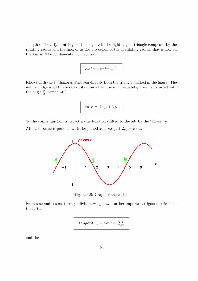
“length of the adjacent leg” of the angle x in the right-angled triangle composed by therotating radius and the sine, or as the projection of the circulating radius, that is now onthe 1-axis. The fundamental connection:

cos2 x+ sin2 x = 1

follows with the Pythagoras Theorem directly from the triangle marked in the figure. Theink cartridge would have obviously drawn the cosine immediately, if we had started withthe angle π

2instead of 0:

cosx = sin(x+ π2).

So the cosine function is in fact a sine function shifted to the left by the “Phase” π2.

Also the cosine is periodic with the period 2π : cos(x+ 2π) = cos x.

Figure 4.6: Graph of the cosine

From sine and cosine, through division we get two further important trigonometric func-tions: the

tangent: y = tanx = sinxcosx

and the

46

cotangent: y = cotx = cosxsinx

= 1tanx

.

Insert: Notations: In the German literature you may often find also

tg x instead of tanx and ctg x instead of cotx.

Figure 4.7: Tangent and cotangent

Tangent and cotangent are periodic with the period π : tan(x+ π) = tan x.

In Chapter 6 we will learn how to calculate the functional value of even the trigonometricfunctions, e.g. of y = sinx for every value of the variable x through elementary calculationssuch as addition and multiplication.

Besides the Pythagoras Relation cos2 x+ sin2x = 1 the

trigonometric addition theorems:

cos(a± b) = cos a cos b∓ sin a sin b

sin(a± b) = sin a cos b± cos a sin b

are of major importance, and experience shows that we have to remind you of them andto recommend that they be learned by heart. In Chapter 8 we will learn to derive themin a much more elegant way than you did in school.

47

Exercise 4.2 Trigonometric Functions:

Sketch the graphs and the definition domains of the following functions, and also the valuedomains except for the last example:a) y = 1 + sinx, b) y = sinx+ cosx, c) y = sinx− cosx, d) y = x+ sinx,e) y = x sinx, f) y = 1

sinx, g) y = 1

tanxund h) y = sinx

x.

4.2.3 Exponential Functions

While raising to powers bn, we have until now introduced only natural numbers n ∈ N asexponents, which indicate how often a real base b occurs as a factor:

bn := b · b · b · . . . · b with n factors b

and we have got the calculation rules:

bnbm = bn+m and (bn)m = bn·m for n,m ∈ N.

We then have added negative exponents by the definition b−n := 1bn

and through theconvention b0 := 1 extended the set of exponents to integers n ∈ Z.

In order to get to the exponential functions we have to allow real numbers x as expo-nents instead of taking only integers n (like with the bases b): y = bx with x, b ∈ R andto restrict ourselves to positive bases b, without changing the calculation rules for thepowers, i.e. with the following

multiplication theorems for exponential functions:

bx+y = bxby, (bx)y = bx·y with x, y, b ∈ R, b > 0

Of central importance for all natural sciences is the natural exponential function withthe irrational number e defined in Section 3.5 as base:

y = ex =: expx,

Its graph with its characteristically fast growth can be directly measured in the followingfigure:

48

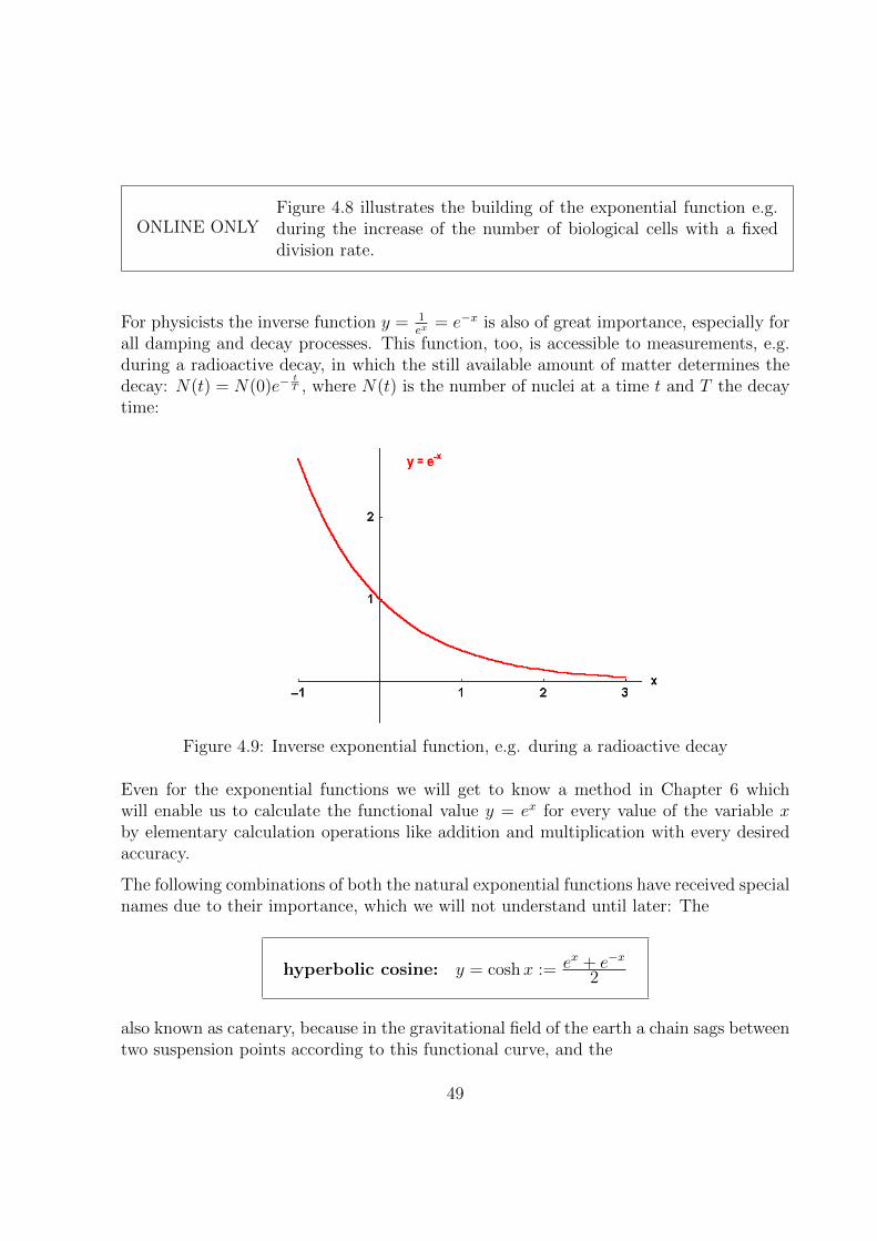
ONLINE ONLYFigure 4.8 illustrates the building of the exponential function e.g.during the increase of the number of biological cells with a fixeddivision rate.

For physicists the inverse function y = 1ex

= e−x is also of great importance, especially forall damping and decay processes. This function, too, is accessible to measurements, e.g.during a radioactive decay, in which the still available amount of matter determines thedecay: N(t) = N(0)e−

tT , where N(t) is the number of nuclei at a time t and T the decay

time:

Figure 4.9: Inverse exponential function, e.g. during a radioactive decay

Even for the exponential functions we will get to know a method in Chapter 6 whichwill enable us to calculate the functional value y = ex for every value of the variable xby elementary calculation operations like addition and multiplication with every desiredaccuracy.

The following combinations of both the natural exponential functions have received specialnames due to their importance, which we will not understand until later: The

hyperbolic cosine: y = coshx := ex + e−x

2

also known as catenary, because in the gravitational field of the earth a chain sags betweentwo suspension points according to this functional curve, and the

49

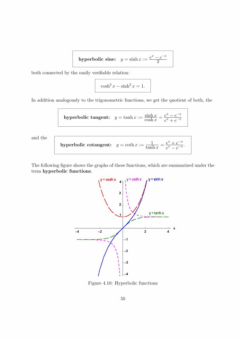
hyperbolic sine: y = sinhx := ex − e−x2

both connected by the easily verifiable relation:

cosh2 x− sinh2 x = 1.

In addition analogously to the trigonometric functions, we get the quotient of both, the

hyperbolic tangent: y = tanhx := sinhxcoshx

= ex − e−xex + e−x

and the

hyperbolic cotangent: y = cothx := 1tanhx

= ex + e−x

ex − e−x .

The following figure shows the graphs of these functions, which are summarized under theterm hyperbolic functions.

Figure 4.10: Hyperbolic functions

50

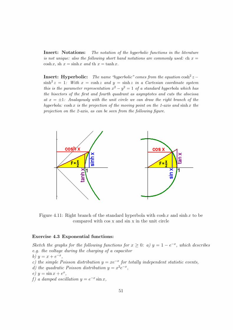
Insert: Notations: The notation of the hyperbolic functions in the literature

is not unique: also the following short hand notations are commonly used: ch x =

coshx, sh x = sinhx and th x = tanhx.

Insert: Hyperbolic: The name “hyperbolic” comes from the equation cosh2 z−sinh2 z = 1: With x = cosh z and y = sinh z in a Cartesian coordinate system

this is the parameter representation x2 − y2 = 1 of a standard hyperbola which has

the bisectors of the first and fourth quadrant as asymptotes and cuts the abscissa

at x = ±1: Analogously with the unit circle we can draw the right branch of the

hyperbola: coshx is the projection of the moving point on the 1-axis and sinhx the

projection on the 2-axis, as can be seen from the following figure.

Figure 4.11: Right branch of the standard hyperbola with coshx and sinh x to becompared with cos x and sin x in the unit circle

Exercise 4.3 Exponential functions:

Sketch the graphs for the following functions for x ≥ 0: a) y = 1 − e−x, which describese.g. the voltage during the charging of a capacitorb) y = x+ e−x,c) the simple Poisson distribution y = xe−x for totally independent statistic events,d) the quadratic Poisson distribution y = x2e−x,e) y = sinx+ ex,f) a damped oscillation y = e−x sinx,

51

g) the reciprocal chain line y = 1coshx

h) the Bose-Einstein distribution function of quantum statistics y = 1ex−1

ori) the corresponding Fermi-Dirac distribution for particles with half-integer spin, e.g. con-ducting electrons y = 1

ex+1,

j) the Planck formula for the spectral intensity distribution of the frequencies of a radiatingcavity y = x3

ex−1.

You may most easily check your sketches online with our function plotter or e.g. graph.tkor www.wolframalpha.com.

4.2.4 Functions with Kinks and Cracks

In addition to these sample functions, physicists use a few functions whose graphs showkinks (or corners) and cracks (or jumps). Among these, the following two are of specialimportance for us:

The first is the

absolute value function: y = |x| :=

x for x ≥ 0−x for x < 0

This function is defined over the whole number axis, but as for the standard parabola thevalue domain covers only the non-negative half-line: y ≥ 0. The following figure showsits graph with the “kink” at x = 0.

Exercise 4.4 Absolute value functions:

Sketch the graphs and the value domains of the following functions:a) y = 1− |x

a|, b) y = x+ |x|, c) y = 1

|x| and d) y = |x| cosx.

The second function is one you most likely have not encountered yet: the Heaviside stepfunction y = θ(x), defined through:

Heaviside step function:

θ(x) := 1 for x > 0,

θ(x) := 0 for x < 0 and

θ(0) :=1

2.

52

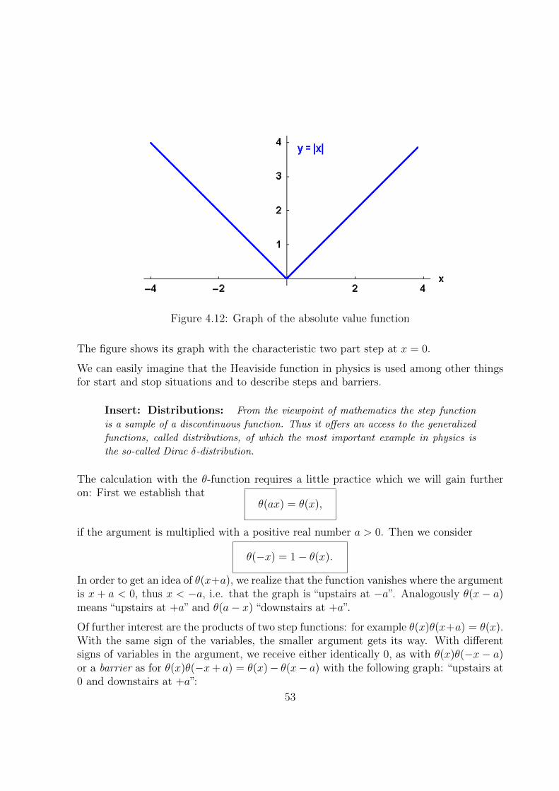
Figure 4.12: Graph of the absolute value function

The figure shows its graph with the characteristic two part step at x = 0.

We can easily imagine that the Heaviside function in physics is used among other thingsfor start and stop situations and to describe steps and barriers.

Insert: Distributions: From the viewpoint of mathematics the step function

is a sample of a discontinuous function. Thus it offers an access to the generalized

functions, called distributions, of which the most important example in physics is

the so-called Dirac δ-distribution.

The calculation with the θ-function requires a little practice which we will gain furtheron: First we establish that

θ(ax) = θ(x),

if the argument is multiplied with a positive real number a > 0. Then we consider

θ(−x) = 1− θ(x).

In order to get an idea of θ(x+a), we realize that the function vanishes where the argumentis x + a < 0, thus x < −a, i.e. that the graph is “upstairs at −a”. Analogously θ(x− a)means “upstairs at +a” and θ(a− x) “downstairs at +a”.

Of further interest are the products of two step functions: for example θ(x)θ(x+a) = θ(x).With the same sign of the variables, the smaller argument gets its way. With differentsigns of variables in the argument, we receive either identically 0, as with θ(x)θ(−x− a)or a barrier as for θ(x)θ(−x+ a) = θ(x)− θ(x− a) with the following graph: “upstairs at0 and downstairs at +a”:

53

Figure 4.13: Heaviside function θ(x) : “upstairs at 0”.

Figure 4.14: Graph of θ(−x): “downstairs at 0”.

Exercise 4.5 Heaviside function: with a>0

a) Sketch θ(−x− a),

b) Sketch θ(x)θ(x− a), θ(−x)θ(−x+ a) and θ(−x)θ(−x− a),

c) Visualize θ(−x)θ(x+ a) = θ(x+ a)− θ(x), θ(−x)θ(x− a)

and θ(x+ a)θ(a− x) = θ(x+ a)− θ(x− a),

d) Draw the graph of θ(x)e−x,

e) Sketch the triangle function (1− |xa|)θ(x+ a)θ(a− x).

Insert: “δ-Function”: The family of functions θa(x) = θ(x+a)θ(a−x)2a with the

family parameter a, the “symmetrical box” of width 2a and height 12a (this means area

1), is one of the large number of function sets, whose limits (here the limit a→ 0)

54

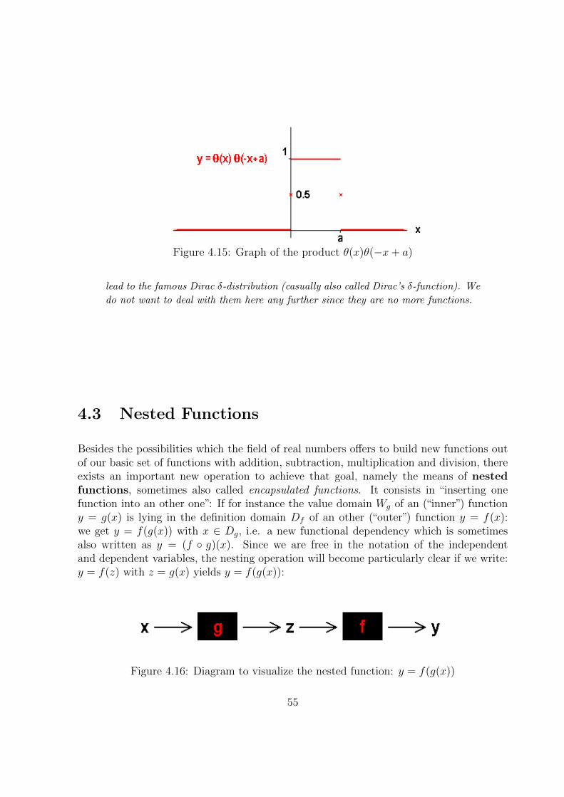
Figure 4.15: Graph of the product θ(x)θ(−x+ a)

lead to the famous Dirac δ-distribution (casually also called Dirac’s δ-function). We

do not want to deal with them here any further since they are no more functions.

4.3 Nested Functions

Besides the possibilities which the field of real numbers offers to build new functions outof our basic set of functions with addition, subtraction, multiplication and division, thereexists an important new operation to achieve that goal, namely the means of nestedfunctions, sometimes also called encapsulated functions. It consists in “inserting onefunction into an other one”: If for instance the value domain Wg of an (“inner”) functiony = g(x) is lying in the definition domain Df of an other (“outer”) function y = f(x):we get y = f(g(x)) with x ∈ Dg, i.e. a new functional dependency which is sometimesalso written as y = (f g)(x). Since we are free in the notation of the independentand dependent variables, the nesting operation will become particularly clear if we write:y = f(z) with z = g(x) yields y = f(g(x)):

Figure 4.16: Diagram to visualize the nested function: y = f(g(x))

55

Simple examples are e.g.: z = g(x) = 1 + x2 with Wg : z ≥ 1 as inner function andy = f(z) = 1

zwith Df = R1 \ 0 as outer one, which yields the Lorentz distribution

function as nested function y = 11+x2

, or z = sinx with Wg : −1 ≤ z ≤ 1 inserted intoy = |x| with Df = R yields y = | sinx| to describe a rectified alternating current, orz = −|2x| with Wg = R inserted into y = ez yields y = exp(−|2x|), an exponential top.Also the bell-shaped Gaussian function y = exp(−x2) built out of z = −x2 with Wg : z ≥ 0and y = ez is an interesting nested function which is widely used in all sciences.

Exercise 4.6 Nested Functions: Sketch the graphs of the above mentioned examplesand examine and sketch the following nested functions:

a) y = sin 2x,b) y = sinx+ sin 2x+ sin 4x,c) y = cos2 x− sin2x,d) y = sin(x2),e) y = sin

(1x

),

f) y = ( sinxx

)2, describing e.g. the intensity of light after diffraction,g) y = tan 2x,h) the classic Maxwell-Boltzmann velocity distribution of the colliding molecules of anideal gas y = x2e−x

2,

i) the Bose-Einstein distribution of the velocities of a gas according to quantum statisticsy = x2

ex2−1,

j) the Fermi-Dirac distribution of the velocities in an electron gas y =√x

ex−a+1with the

constant a depending on the temperature,k) Planck’s formula for the spectral intensity of the wavelengths of the radiation of a cavityy = 1

x5[e1x−1]

,

l) y = esinx,m) y = 1− |2x| andn) y = 1

|2x| .

You may easily check your sketches with our online function plotter ore.g. graph.tk or www.wolframalpha.com.

56

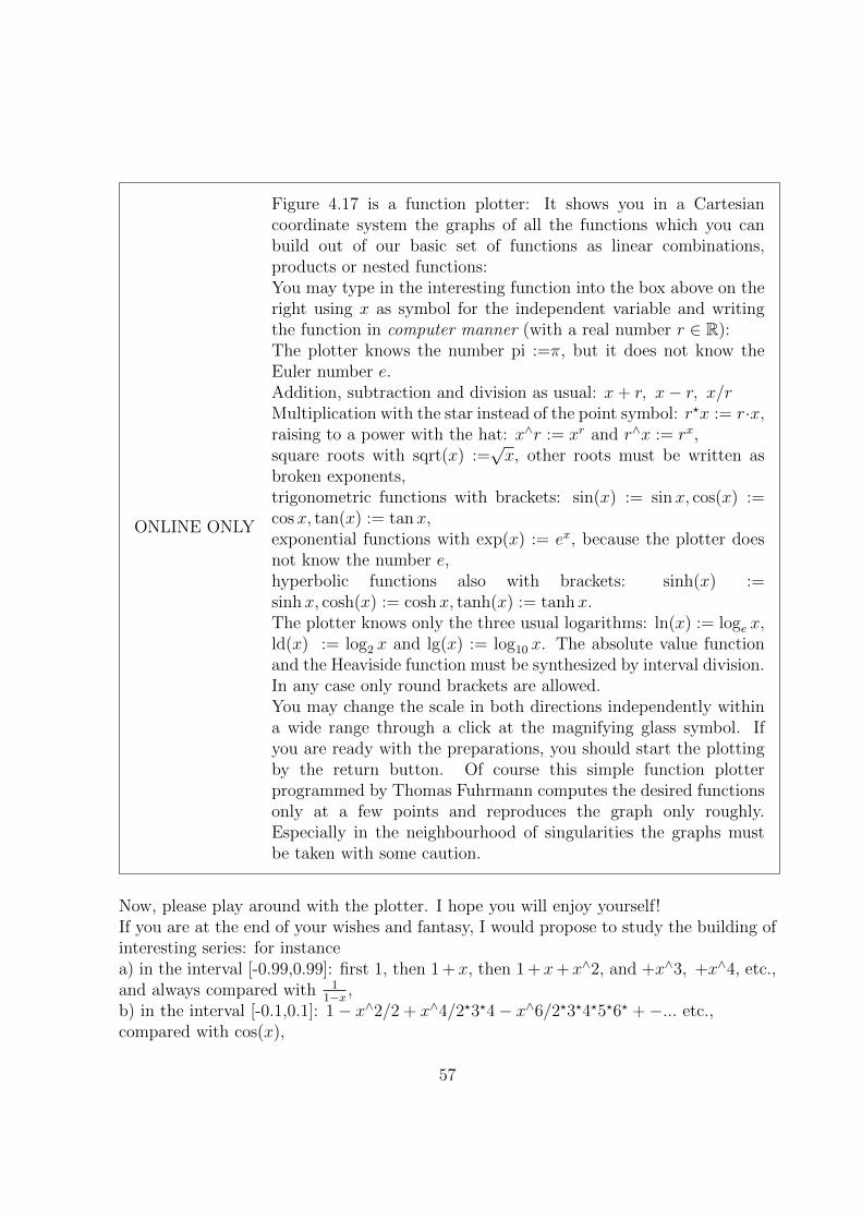
ONLINE ONLY

Figure 4.17 is a function plotter: It shows you in a Cartesiancoordinate system the graphs of all the functions which you canbuild out of our basic set of functions as linear combinations,products or nested functions:You may type in the interesting function into the box above on theright using x as symbol for the independent variable and writingthe function in computer manner (with a real number r ∈ R):The plotter knows the number pi :=π, but it does not know theEuler number e.Addition, subtraction and division as usual: x+ r, x− r, x/rMultiplication with the star instead of the point symbol: r?x := r·x,raising to a power with the hat: x∧r := xr and r∧x := rx,square roots with sqrt(x) :=

√x, other roots must be written as

broken exponents,trigonometric functions with brackets: sin(x) := sin x, cos(x) :=cosx, tan(x) := tan x,exponential functions with exp(x) := ex, because the plotter doesnot know the number e,hyperbolic functions also with brackets: sinh(x) :=sinhx, cosh(x) := cosh x, tanh(x) := tanh x.The plotter knows only the three usual logarithms: ln(x) := loge x,ld(x) := log2 x and lg(x) := log10 x. The absolute value functionand the Heaviside function must be synthesized by interval division.In any case only round brackets are allowed.You may change the scale in both directions independently withina wide range through a click at the magnifying glass symbol. Ifyou are ready with the preparations, you should start the plottingby the return button. Of course this simple function plotterprogrammed by Thomas Fuhrmann computes the desired functionsonly at a few points and reproduces the graph only roughly.Especially in the neighbourhood of singularities the graphs mustbe taken with some caution.

Now, please play around with the plotter. I hope you will enjoy yourself!If you are at the end of your wishes and fantasy, I would propose to study the building ofinteresting series: for instancea) in the interval [-0.99,0.99]: first 1, then 1 + x, then 1 + x+ x∧2, and +x∧3, +x∧4, etc.,and always compared with 1

1−x ,b) in the interval [-0.1,0.1]: 1− x∧2/2 + x∧4/2?3?4− x∧6/2?3?4?5?6? +−... etc.,compared with cos(x),

57

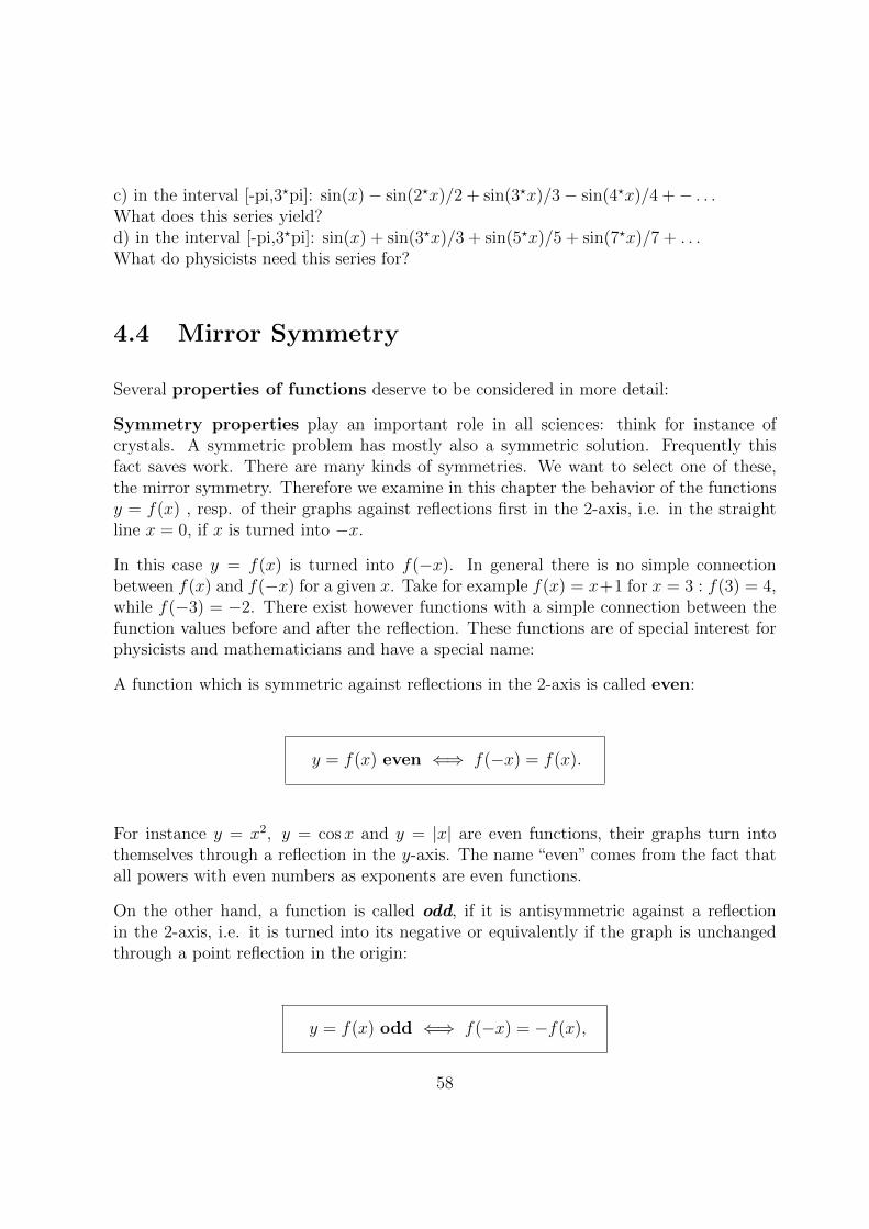
c) in the interval [-pi,3?pi]: sin(x)− sin(2?x)/2 + sin(3?x)/3− sin(4?x)/4 +− . . .What does this series yield?d) in the interval [-pi,3?pi]: sin(x) + sin(3?x)/3 + sin(5?x)/5 + sin(7?x)/7 + . . .What do physicists need this series for?

4.4 Mirror Symmetry

Several properties of functions deserve to be considered in more detail:

Symmetry properties play an important role in all sciences: think for instance ofcrystals. A symmetric problem has mostly also a symmetric solution. Frequently thisfact saves work. There are many kinds of symmetries. We want to select one of these,the mirror symmetry. Therefore we examine in this chapter the behavior of the functionsy = f(x) , resp. of their graphs against reflections first in the 2-axis, i.e. in the straightline x = 0, if x is turned into −x.

In this case y = f(x) is turned into f(−x). In general there is no simple connectionbetween f(x) and f(−x) for a given x. Take for example f(x) = x+1 for x = 3 : f(3) = 4,while f(−3) = −2. There exist however functions with a simple connection between thefunction values before and after the reflection. These functions are of special interest forphysicists and mathematicians and have a special name:

A function which is symmetric against reflections in the 2-axis is called even:

y = f(x) even ⇐⇒ f(−x) = f(x).

For instance y = x2, y = cosx and y = |x| are even functions, their graphs turn intothemselves through a reflection in the y-axis. The name “even” comes from the fact thatall powers with even numbers as exponents are even functions.

On the other hand, a function is called odd, if it is antisymmetric against a reflectionin the 2-axis, i.e. it is turned into its negative or equivalently if the graph is unchangedthrough a point reflection in the origin:

y = f(x) odd ⇐⇒ f(−x) = −f(x),

58

for instance y = 1x, y = x3 or y = sinx.

The straight line function y = s · x + c is for c 6= 0 neither even nor odd. Every functioncan however be split into an even and an odd part:

f(x) = f(x)+f(−x)2

+ f(x)−f(−x)2

= f+(x) + f−(x) with the

even part: f+(x) =f(x) + f(−x)

2 = f+(−x)

and the

odd part: f−(x) =f(x)− f(−x)

2 = −f−(−x).

For instance c is the even part of the straight line function y = s · x + c and s · x is theodd part.

Exercise 4.7 Symmetry properties of functions:

1) Examine the following functions for mirror symmetry:a) y = x4, b) y = x5, c) y = sinx

x, d) y = tanx, e) y = cotx,

f) y = sinhx, g) y = coshx and h) y = −|x|.2) Determine the even and odd part of e.g.:a) f(x) = x(x+ 1), b) f(x) = x sinx+ cosx, c) y = ex and d) y = θ(x).

4.5 Boundedness

Our next step is to transfer the boundedness, known to us from sequences, onto functions.A function is said to be bounded above in an interval [a, b], if there is an upper bound forthe functional values in this interval:

y = f(x) bounded above in [a, b] ⇐⇒ ∃B : B ≥ f(x) ∀x ∈ [a, b]

59

Bounded below is defined analogously with the lower bound A ≤ f(x).The standard parabola y = x2 for example and the absolute value function y = |x| arebound below through A = 0 and the step function θ(x) is bounded above through B = 1and bounded below through A = 0.

Exercise 4.8 Boundedness:

Examine the following functions for boundedness within their definition domain in R:a) y = 2− 2x2, b) y = x2 − 2x− 3, c) y = 2x−3

x−1, d) y = sinx+ cosx,

e) y = x sinx, f) y = 1− e−x, g) y = x+ e−x, h) y = xe−x,i) y = x2e−x, j) y = e−x sinx and k) y = 1

|x| .

4.6 Monotony

Also monotony can be transferred from sequences onto functions, since sequences can beunderstood as special functions over the definition domain N:

A function is said to be monotonically increasing in the interval [a, b], if with increasingargument the functional values also increase in the interval [a, b]:

y = f(x) monotonically increasing in [a, b]⇐⇒ x1, x2 ∈ [a, b] ∈ Df : x1 < x2 ⇒ f(x1) ≤ f(x2)

For example is y = sx+ c for s > 0 monotonically increasing.

Monotonically decreasing is analogously defined with f(x1) ≥ f(x2), for instance y = 1x

in its definition domain Df is monotonically decreasing.If even f(x1) < f(x2) holds true for all x1, x2 ∈ D with x1 < x2, we call the functionstrictly monotonic increasing as in the case of sequences. In both previous examples themonotony is strict.

Exercise 4.9 Monotonic functions:

Examine the following functions for monotony:a) y = x2, b) y = x3

3− 3, c) y = 2x−3

x−1,

d) y = sinx in [−π2, π

2], e) y = tanx in [−π

2, π

2],

f) y = cosx in [0, π], g) y = 1− e−x, h) y = sinhx,i) y = coshx and j) y = θ(x).

60

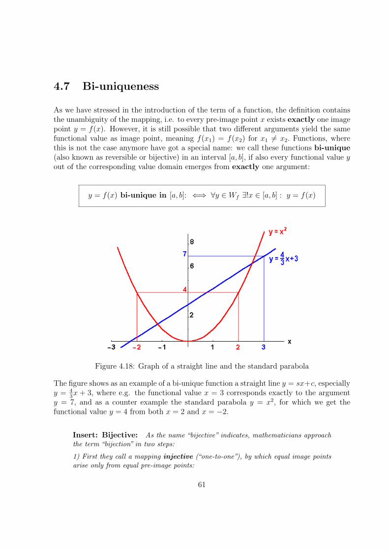
4.7 Bi-uniqueness

As we have stressed in the introduction of the term of a function, the definition containsthe unambiguity of the mapping, i.e. to every pre-image point x exists exactly one imagepoint y = f(x). However, it is still possible that two different arguments yield the samefunctional value as image point, meaning f(x1) = f(x2) for x1 6= x2. Functions, wherethis is not the case anymore have got a special name: we call these functions bi-unique(also known as reversible or bijective) in an interval [a, b], if also every functional value yout of the corresponding value domain emerges from exactly one argument:

y = f(x) bi-unique in [a, b]: ⇐⇒ ∀y ∈ Wf ∃!x ∈ [a, b] : y = f(x)

Figure 4.18: Graph of a straight line and the standard parabola

The figure shows as an example of a bi-unique function a straight line y = sx+c, especiallyy = 4

3x + 3, where e.g. the functional value x = 3 corresponds exactly to the argument

y = 7, and as a counter example the standard parabola y = x2, for which we get thefunctional value y = 4 from both x = 2 and x = −2.

Insert: Bijective: As the name “bijective” indicates, mathematicians approachthe term “bijection” in two steps:

1) First they call a mapping injective (“one-to-one”), by which equal image pointsarise only from equal pre-image points:

61

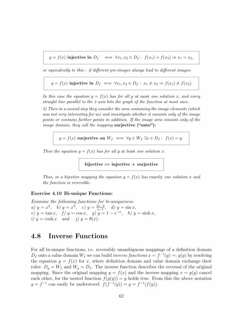
y = f(x) injective in Df ⇐⇒ ∀x1, x2 ∈ Df : f(x1) = f(x2)⇒ x1 = x2,

or equivalently to this : if different pre-images always lead to different images:

y = f(x) injective in Df ⇐⇒ ∀x1, x2 ∈ Df : x1 6= x2 ⇒ f(x1) 6= f(x2).

In this case the equation y = f(x) has for all y at most one solution x, and everystraight line parallel to the 1-axis hits the graph of the function at most once.

2) Then in a second step they consider the area containing the image elements (whichwas not very interesting for us) and investigate whether it consists only of the imagepoints or contains further points in addition. If the image area consists only of theimage domain, they call the mapping surjective (“onto”):

y = f(x) surjective on Wf ⇐⇒ ∀y ∈Wf ∃x ∈ Df : f(x) = y.

Then the equation y = f(x) has for all y at least one solution x.

bijective := injective + surjective

Thus, in a bijective mapping the equation y = f(x) has exactly one solution x and

the function is reversible.

Exercise 4.10 Bi-unique Functions:

Examine the following functions for bi-uniqueness:a) y = x2, b) y = x3, c) y = 2x−3

x−1, d) y = sinx,

e) y = tanx, f) y = cosx, g) y = 1− e−x, h) y = sinhx,i) y = coshx and j) y = θ(x).

4.8 Inverse Functions

For all bi-unique functions, i.e. reversibly unambiguous mappings of a definition domainDf onto a value domain Wf we can build inverse functions x = f−1(y) =: g(y) by resolvingthe equation y = f(x) for x, where definition domain and value domain exchange theirroles: Dg = Wf and Wg = Df . The inverse function describes the reversal of the originalmapping. Since the original mapping y = f(x) and the inverse mapping x = g(y) canceleach other, for the nested function f(g(y)) = y holds true. From this the above notationg = f−1 can easily be understood: f(f−1(y)) = y = f−1(f(y)).

62

Insert: Function Symbol: With a closer look, the symbol f has two different

meanings:

1) On the one hand f gives the operation, which creates the function values y out

of the arguments x. If we write f−1, we mean the reversal of this operation.

2) On the other hand the term f(x) means the special function value, which emerges

from a certain value x of the variable by this prescription. The inverse of this

function value is denoted by 1f(x) = (f(x))−1. f−1(x) is the function value of the

inverse function. E.g. sin 1 = 0.84, (sin 1)−1 = 1.188, but sin−1 1 = arcsin 1 =

1.57.

In the sense of our physical definition of the function as input-output relation, with theinverse function input and output are interchanged, i.e. the flow direction arrows in ourfigure are simply reversed.

Figure 4.19: Black boxes for y = f(x) and the inverse function x = g(y)

Inverse functions occur very often in physics. As an example we consider the length L ofthe liquid column in a narrow glass pipe as function of temperature T : L = f(T ). If weuse the glass pipe as thermometer to measure the temperature, we observe the length ofthe liquid column and infer from it the temperature T = g(L).

Usually after the solution of the equation y = f(x) for x has been found, the now inde-pendent variable y is renamed x and the dependent one y. For the graph the transitionto the inverse function simply means the reflection in the straight line y = x, i.e. thebisector of the first and third quadrant. In this manner we receive a new function out ofevery bi-unique function.

An instructive example is the standard parabola y = x2. Only through the limitationof the definition domain to x ≥ 0 does it become a bi-unique function which is reversible:The inverse function is a new function for us, the square root function x = +

√y and

after renaming the variables: y = +√x = x

12 . Through the notation with the fraction

in the exponent, powers were defined also for rational exponents, beyond our earlierconsiderations, without any change in the calculation rules for powers.

The possibility to create new functions by inversion out of bi-unique functions enlargesthe treasure of our basic set of functions introduced in section 4.2 (rational, trigonometric,and exponential functions) nearly to twice as much. We want to devote ourselves now tothis task:

63

Figure 4.20: The standard parabola y = x2 and its reflection in the bisector deliveringthe inverse function: the square root function y = +

√x

4.8.1 Roots

The example of the parabola has already shown to us that the inverse functions of thepowers y = xn with integer exponents n ∈ Z are the root functions with fractions asexponents: x = y

1n , rewritten as: y = n

√x = x

1n where however the even-numbered powers

need to be made bi-unique before the reversal through limitation of the domain to x ≥ 0.

As inverse functions of the polynomials we receive more complicated roots: for examplefrom y = x2 + 1 which is bi-unique for x ≥ 0, we find x =

√(y − 1) and after redefinition

y =√

(x− 1).

Exercise 4.11 Inverse functions:

Determine the inverse functions of the following functions:a) y = −2x− 2, b) y = 2− 2x2, c) y = x2 − 2x− 3, d) y = x3

3− 3,

e) y = 1(1−x)

and f) y = 1x2−1

.

4.8.2 Cyclometric Functions

The trigonometric functions y = sin x or y = cos x are periodic in x with the period 2πand y = tanx or y = cotx with the period π. Thus they are by no means bi-uniquefunctions. Only by limitation of the definition domain can reversibility be achieved.

For the odd functions y = sinx, y = tanx and cot x we usually choose−π

2< x ≤ π

2, for the even one y = cosx 0 < x ≤ π. Due to the periodicity we

64

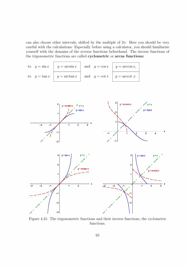
can also choose other intervals, shifted by the multiple of 2π. Here you should be verycareful with the calculations: Especially before using a calculator, you should familiarizeyourself with the domains of the reverse functions beforehand. The inverse functions ofthe trigonometric functions are called cyclometric or arcus functions:

to y = sinx y = arcsinx and y = cosx y = arccosx,

to y = tanx y = arctanx and y = cotx y = arccot x.

Figure 4.21: The trigonometric functions and their inverse functions, the cyclometricfunctions.

65

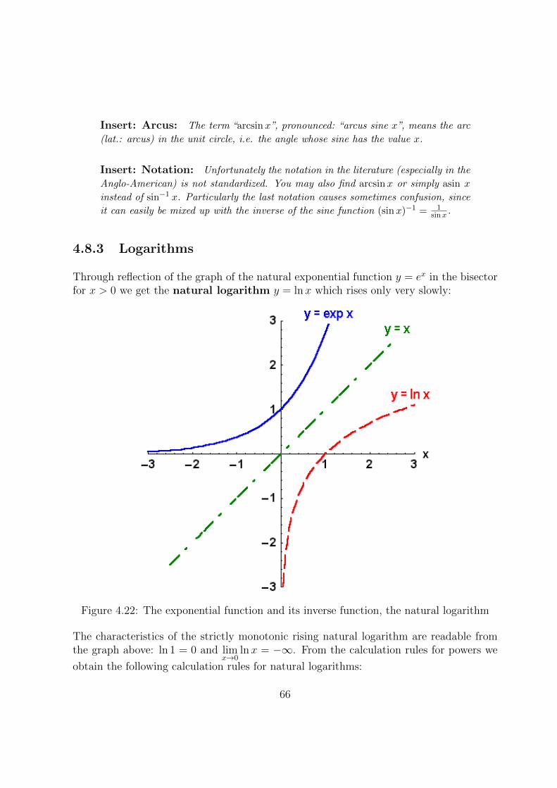
Insert: Arcus: The term “arcsinx”, pronounced: “arcus sine x”, means the arc

(lat.: arcus) in the unit circle, i.e. the angle whose sine has the value x.

Insert: Notation: Unfortunately the notation in the literature (especially in the

Anglo-American) is not standardized. You may also find arcsinx or simply asin x

instead of sin−1 x. Particularly the last notation causes sometimes confusion, since

it can easily be mixed up with the inverse of the sine function (sinx)−1 = 1sinx .

4.8.3 Logarithms

Through reflection of the graph of the natural exponential function y = ex in the bisectorfor x > 0 we get the natural logarithm y = lnx which rises only very slowly:

Figure 4.22: The exponential function and its inverse function, the natural logarithm

The characteristics of the strictly monotonic rising natural logarithm are readable fromthe graph above: ln 1 = 0 and lim

x→0lnx = −∞. From the calculation rules for powers we

obtain the following calculation rules for natural logarithms:

66

ln y · z = ln y + ln z, ln(yz) = ln y − ln z and ln(zy) = y ln z .

After having become familiar with especially the natural exponential function and the nat-ural logarithm, we can use this knowledge to define the general exponential function:

general exponential function: y = bx := ex ln b for b > 0

and as its inverse function the general logarithm:

general logarithm: y = logb x := lnxln b

,

which for b > 1 (just as for lnx) rises strictly monotonic, for b < 1 however decreasesmonotonically.

Figure 4.23: The three most important logarithms for the bases: 2, e, and 10

As calculation rules for the general logarithms with unchanged base b we get:

logb yz = logb y + logb z, logb(yz) = logb y − logb z and y logb z = logb(z

y) .

67

Besides the very important natural logarithms ln := loge with the irrational number

e = 2.7182. . . as base, there are simplified notations for two further widely used bases: the

binary lb:= log2 or dual ld:= log2 and the common or Brigg’s logarithms with

the base 10 lg:= log10 .

The conversion between logarithms with different bases follows from the formula:

logb y = logb z · logz y

especially, e.g. for b = 10 and y = x:

lgx =lg e lnx = 0.434 lnx,

since through the triple use of the identity

b logb x = 2 ldx = e ln x = 10 lg x = x

we get b logb y = y = z logz y = (b logb z)logz y = b logb z· logz y and thus the exponents are equal.

Exercise 4.12 Logarithms:

a) What is logb b?

b) Show that ln 10 = 1lge or rather ln 2 = 1

lbe .

c) Calculate lbx from lnx.d) Calculate 2.5 2.5.

Also the general power function is defined with the help of the natural exponentialfunction and the natural logarithm for x > 0 and r ∈ R through:

general power function: y = xr = e rlnx for x > 0 and r ∈ R.

68

Figure 4.24: Power functions

We will not use it very often.

The inverse functions of the hyperbolic functions: coshx, sinhx and tanh x, which wehave built out of natural exponential functions are more important for physics: They arecalled area functions, can obviously be expressed through natural logarithms and aredisplayed in the following figure:

to y = coshx := ex + e−x

2 y = arcosh x = ln(x+√x2 − 1

),

to y = sinhx := ex − e−x2 y = arsinh x = ln

(x+√x2 + 1

),

to y = tanhx := ex − e−xex + e−x

y = artanh x = 12 ln 1 + x

1− x .

Insert: Notations: Also in this case, there are notation difficulties like with

the inverse functions of the trigonometric functions: arsinh x = arcsinh x = arsh

x = sinh−1x, etc.

69

Figure 4.25: The hyperbolic functions and their inverse functions, the area functions

Insert: Area: The name “arcosh x”, i.e. “area hyperbolic cosine x”,

comes from the connection with the area (also lat.: area) of a sector of the standard

hyperbola: It can be shown that y is the square measure of the area of the hyperbola

sector which in Figure 4.11 is dyed (between the origin, the moving point, the vertex,

and the moving point reflected at the 1-axis), if the 1-coordinate of the moving point

(which means the hyperbolic cosine equals x).

70

Exercise 4.13 Area functions:

a) Show that from y = ln(x+√x2 + 1

)follows x = sinh y.

b) Show that from y = 12

ln 1+x1−x follows x = tanh y.

4.9 Limits

The calculation of limits for functions is reduced to our limiting procedure for sequencesby the following consideration: Whenever we want to know whether the functional valuesf(x) of a real function f tend to a number y0 when the arguments x0 approach a realnumber x0, we choose a sequence (xn)n∈N ⊆ Df of real numbers within the definitiondomain Df of the function f , which for n → ∞ tends to the number x0 ∈ Df . Thenwe calculate the functional values f(xn) for these arguments, which once again form asequence (f(xn))n∈N, and check whether this sequence of the functional values convergesto y0. If this holds true for every sequence taken out of the domain and converging to x0

then we call such sequence of functional values convergent to y0 : limx→x0

f(x) = y0 :

limx→x0

f(x) = y0 convergent: ⇐⇒ ∀(xn)n∈N : limn→∞

xn = x⇒ limn→∞

f(xn) = y0

If we modify our definition for the convergence of sequences, we find:

limx→x0

f(x) = y0 convergent: ⇐⇒ ∀ε > 0 ∃δ > 0 :

|f(x)− y0| < ε ∀x ∈ Df with|x− x0| < δ

To show this for all sequences is easier said than done! We do not need however to occupyourselves with these partly difficult mathematical questions which you will have enoughopportunity to deal with in the analysis lecture. Instead we shall be content with someexamples which are important for physicists.

Already from the graphs we can see e.g. for the behaviour at the origin that for the

powers limx→0

xn = 0 while limx→0

x−n divergent is divergent for n ∈ N. Moreover we

can clearly see that limx→0

cosx = 1 and limx→0

sinx = 0 .

71

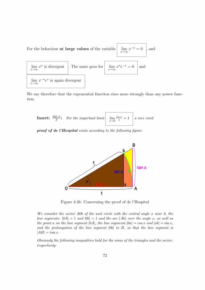
For the behaviour at large values of the variable limx→∞

x−n = 0 , and

limx→∞

xn is divergent . The same goes for limx→∞

xne−x = 0 and

limx→∞

x−nex is again divergent .

We say therefore that the exponential function rises more strongly than any power func-tion.

Insert: sinxx : For the important limit lim

x→0

sinxx = 1 a nice vivid

proof of de l’Hospital exists according to the following figure:

Figure 4.26: Concerning the proof of de l’Hospital

We consider the sector A0b of the unit circle with the central angle x near 0, theline segments: |0A| = 1 and |0b| = 1 and the arc (Ab) over the angle x, as well asthe point a on the line segment |0A|, the line segments |0a| = cosx and |ab| = sinx,and the prolongation of the line segment |0b| to B, so that the line segment is|AB| = tanx.

Obviously the following inequalities hold for the areas of the triangles and the sector,

respectively:

72

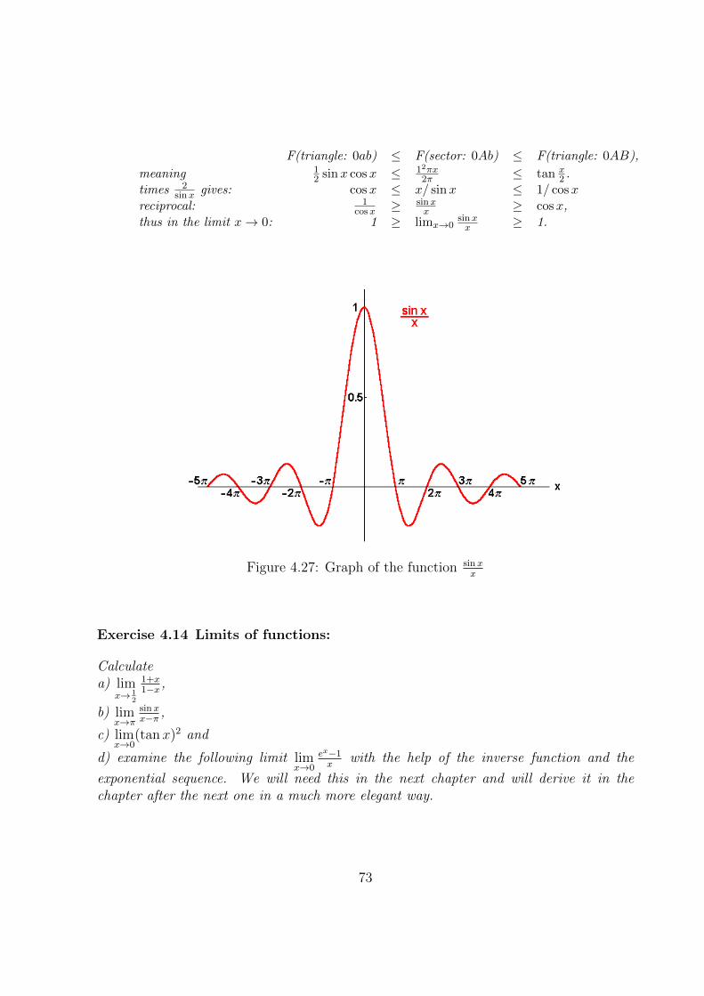
F(triangle: 0ab) ≤ F(sector: 0Ab) ≤ F(triangle: 0AB),

meaning 12 sinx cosx ≤ 12πx

2π ≤ tan x2 .

times 2sinx gives: cosx ≤ x/ sinx ≤ 1/ cosx

reciprocal: 1cosx ≥ sinx

x ≥ cosx,

thus in the limit x→ 0: 1 ≥ limx→0sinxx ≥ 1.

Figure 4.27: Graph of the function sinxx

Exercise 4.14 Limits of functions:

Calculatea) lim

x→ 12

1+x1−x ,

b) limx→π

sinxx−π ,

c) limx→0

(tanx)2 and

d) examine the following limit limx→0

ex−1x

with the help of the inverse function and the

exponential sequence. We will need this in the next chapter and will derive it in thechapter after the next one in a much more elegant way.

73

4.10 Continuity

The last important property of functions which we need is continuity: Particularly inclassical physics we often take the viewpoint: “natura non facit saltus” (nature does notjump), i.e. we deal with continuous functions. For many experiments continuity is un-avoidable because of the finite accuracy of measurements. But there are also discontinuousprocesses in nature, e.g. switching on or off, and “quantum leaps”.

Mathematicians define a function as continuous at a point x0 if it maps points in theneighbourhood of x0 to other neighbouring points, in shorthand:

y = f(x) continuous at x0 ⇐⇒ ∀ε > 0 ∃δ(ε) > 0 : |f(x)− y0| < ε ∀x with |x− x0| < δ

For limits this means that at the considered point x0 the right-hand limit and the left-hand one are equal and are given by the function value y0 = f(x0) of the limit x0 of asequence xn out of the definition domain of the arguments:

limx→x0+0

f(x) = limx→x0−0

f(x) =: limx→x0

f(x) = y0 = f(x0) = f( limn→∞

xn).

The graph of a continuous function “does not jump”. The Heaviside function is the func-tion with the “unit jump”. With its help all discontinuities occurring in physics can bedescribed. Sums, differences, products, quotients, and nested functions of continuous func-tions are again continuous. Therefore all functions considered until now apart from theHeaviside step function are continuous within their definition domains. The step functionjumps at the point 0 by an amount of 1: lim

x→0+0θ(x) = 1, lim

x→0−0θ(x) = 0 while θ(0) = 1

2.

The standard hyperbola y = 1x

is admittedly discontinuous at the point x = 0, but it isnot defined there.

Exercise 4.15 Continuous functions:

Check the continuity of the following functions at the origin x0 = 0:a) y = x, b) y = x2, c) y = 1

1−x , d) y = x sinx, e) y = x+ e−x,

f) y = sinxx

, g) y = ex−1x

, h) y = |x|, i) y = θ(x+ a)θ(a− x),j) y = θ(x)θ(−x− a) k) y = θ(x)e−x and l) y = θ(x)xe−x.

74

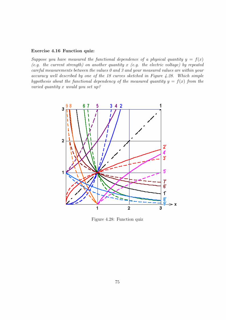
Exercise 4.16 Function quiz:

Suppose you have measured the functional dependence of a physical quantity y = f(x)(e.g. the current strength) on another quantity x (e.g. the electric voltage) by repeatedcareful measurements between the values 0 and 3 and your measured values are within youraccuracy well described by one of the 18 curves sketched in Figure 4.28. Which simplehypothesis about the functional dependency of the measured quantity y = f(x) from thevaried quantity x would you set up?

Figure 4.28: Function quiz

75

Chapter 5

DIFFERENTIATION

It is hardly an overstatement to claim that theoretical physics began with the concept ofdifferentiation. The development of this branch of mathematics by Leibniz and Newtonin the 17th century made possible the formulation of the exact laws describing a widerange of very important physical phenomena: Newton’s laws of mechanics, the Maxwellequations for electrodynamics and the Schrodinger equation of quantum mechanics areall expressed in the language of differential equations. The solutions of these requirethe entire apparatus of analysis, especially of the differential and integral calculus. Forthis reason the present chapter is of the utmost importance to us. Differentiation andintegration are indispensable tools of every physicist.

5.1 Differential quotient

We first examine the uniform motion of a particle along a straight line. Thereby, thedistance covered is: x(t) = st + x0 as a function of time t, where x0 = x(0) means theposition at the time t = 0.

77

Figure 5.1: The straight line x(t) = st+ x0

Physicists are first of all interested in the velocity of the motion. From the graphof this linear function, an ascending straight line with the gradient s through the point(0, x0), we extract the velocity v as quotient of the covered distance x(t) − x(0) dividedby the time needed t, which gives us exactly

v =x(t)− x0

t= s,

the gradient. It is therefore the gradient of the graph, which interests us. For thestraight line we obviously could have taken an other time interval t2 − t1, too:

v =x(t2)− x(t1)

t2 − t1and received the same result. Because with a uniform motion equal distances are coveredwithin equal time intervals: the velocity is constant. We mark the differences in numeratorand denominator of the quotient in the following way through upper-case Greek deltas:(x(t2) − x(t1)) =: ∆x(t) and (t2 − t1) =: ∆t and call the quotient of both differencequotient:

v =∆x(t)

∆t.

Generally, when the independent variable is called x again, we receive for the

78

difference quotient:∆f(x)

∆x :=f(x2)− f(x1)

x2 − x1

How will the situation change, if we consider in our physical example a general motionalong our straight line with a time varying velocity, which is displayed through an arbitraryfunction of the distance from time x(t)?

Figure 5.2: Graph of an arbitrary function x(t) of time

Through the figure we recognize that the difference quotient gives the gradient of thesecant, which connects the two points (t1, x(t1)) and (t2, x(t2)). The value of the differencequotient is then

vm =∆x(t)

∆t=x(t2)− x(t1)

t2 − t1,

the middle or average velocity during the time interval ∆t. For many purposes the av-erage velocity plays an important role. In physics however, the instantaneous velocity,say at the time t1, is far more important. We get it from the average velocity between t1and t2 by the limit in which t2 approaches t1. This limit is called the differential quotient.

79

5.2 Differential Quotient

In order to determine the instantaneous velocity for example at the time t0, we choosean arbitrary point in time t = t0 + ∆t near t0 and draw the secant through the functionvalues x(t) = x(t0) + ∆x(t) and x(t0) = x0. Then we determine their gradient as the

difference quotient s = ∆x(t)∆t

= x(t)−x(t0)t−t0 and let the time point t tend to t0, i.e. let

∆t→ 0. With this procedure for a continuous function also x(t) tends to x0 = x(t0) andthe secant becomes the tangent to the graphs with the

tangent gradient:dx

dt

∣∣∣∣t0

= lim∆t→0

∆x

∆t

In our usual mathematical terminology with x for the independent and y = f(x) for thedependent variable, the results is

differential quotient:df(x)dx

∣∣∣∣x0

= lim∆x→0

f(x0 + ∆x)− f(x0)∆x

The difference quotient ∆y∆x≡ ∆f(x)

∆x≡ f(x0+∆x)−f(x0)

∆xhas turned into the so-called differen-

tial quotient through this limit ∆x → 0, denoted by its inventor Leibniz with df(x)dx

∣∣x0

ordydx

∣∣x0

, which is however, at first sight not quotient itself, but only the limit of a quotient.Just as for all with all fundamental terms in mathematics there are several notationsfor it: The alternative notation which most of you are familiar with from school, f ′(x0),spoken “f prime at the point x0”, was proposed by Lagrange and serves as a reminderthat the gradient of the graph, also called (first) derivative of a function, in general isitself again a new function varying along the curve of the independent variable x, hereespecially given at the point x0. Also the term

(ddx

)f(x)

∣∣x0

is used which emphasizes that

the differentiation is an “operation” where the “differential operator”(ddx

)is to act on the

function f(x) standing to the right of it, and the result should be evaluated especially atthe point x = x0. It makes sense to have all these notations available, and to use thenotation that is most convenient for one’s purpose.

Equivalent denotations: f ′(x0) ≡ df(x)dx

∣∣x0≡(ddx

)f(x)

∣∣x0≡(dydx

) ∣∣x0

Hereby, we have to mention a curiosity of physicists: If the independent variable is thetime t, as of course happens quite often, physicists write and speak a high-placed “point”˙ instead of the “prime” ′: x(t0) ≡ dx(t)

dt

∣∣t0

.

80

Insert: Linear Approximation: We have seen that the differential quotientof a function f(x) at a point x0 has a nice vivid meaning: it gives us the gradientof the tangent to the graph of the function at the point x0. We may understand thistangent property also in the following way:

We set ourselves the task of approximating the curve described by the functiony = f(x) in the neighborhood of the point x0 as nearly as possible by a straightline g(x) = sx+ a: For this purpose we demand therefore:

1. At the point x0, there should hold f(x0) = g(x0) = sx0 + a, from which theabsolute term a = −sx0 + f(x0) can be determined. Inserted above this gives:g(x) = s(x− x0) + f(x0). Thus we find for the deviation of the approximating lineg from the curve f :

f(x)− g(x) = f(x)− f(x0)− s∆x

with the distance ∆x := x− x0 of the independent variable from the approximationpoint.

2. This deviation of the approximation line g from the curve f, measured by ∆x :

f(x)− g(x)

∆x=f(x)− f(x0)

∆x− s

should vanish in the limit x tending to x0, i.e. ∆x→ 0. But this means exactly:

lim∆x→0

f(x)− f(x0)

∆x− s = f ′(x0)− s = 0 and thus s = f ′(x0).

Therefore, we get the best linear approximation to the graph of the function f(x)in the neighbourhood of the point x0, if we choose a straight line with the differential

quotient as gradient, and this is of course exactly the definition of the tangent.

Insert: Differentials: To become even more acquainted with the importantconcept of the differential quotient, we want to study as a further alternative accessthe term “differential”. Here nothing really new will be obtained. We only get newinsight in the concept already obtained. This insight will be useful for later appli-cations and extensions, since it can easily be transferred to several dimensions andwill only there display its full power:

We avoid deliberately the limit and write

the difference quotient as an equation: ∆f(x)∆x

∣∣x0

= f ′(x0) +Rf(x0,∆x)

with a remainder Rf (x0,∆x), which depends on the function f, the point x0 and theinterval ∆x, and vanishes with ∆x. If we multiply this difference quotient with theincrease of the variable ∆x, we get

the “real increase” of our function at x0: ∆f(x)∣∣x0

= f ′(x0)∆x+ rf (x0,∆x)

81

with the new remainder rf (x0,∆x) = Rf (x0,∆x)∆x, which apparently vanisheseven more strongly than Rf does with ∆x. If we can ignore this remainder, we findfor the real increase of the function ∆f(x)

∣∣x0

a first approximation linear in ∆x,

the “linear part of the increase of the function” df(x)∣∣x0

= f ′(x0)∆x,

which is called the “differential”.

In particular for the function y = f(x) = x, the bisector line, we get because off ′(x) = 1

the linear part of the linear function of the independent variable: dx = ∆x,

which is not necessarily infinitesimal and which we may insert above in order to get(using the Lagrange or Leibniz form of the differential quotient):

differential:

df(x) = f ′(x)dx ≡(dfdx

)dx, linear part of the increase of

the function.

Thus we have got an equation in which the symbols df and dx, having been defined

only as quotient in the Leibniz form of the differential quotient, now appear as

singles, as “linear parts of the increase” and are defined also as non-infinitesimal

quantities. Because of this possibility we prefer the far sighted and suggestive writing

form for the differential quotient by Leibniz to that of Lagrange known to most of

you from school.

5.3 Differentiability

From the above construction of the differential quotient as limit of the difference quotientand our knowledge about the formation of limits, it follows immediately that we cannotdetermine a gradient for every function at every point, meaning not every function isdifferentiable at every point of its definition domain:

f(x) differentiable at x0 :⇐⇒ the limit of the difference quotient exists.

82

For this we have to require that both the “limit from the right” limx→x+0

f(x)−f(x0)x−x0 , for which

like above in Figure 5.2 we have chosen the second point for the secant to the right of x0,and the “limit from the left” lim

x→x−0

f(x)−f(x0)x−x0 with the second secant point x to the left of

x0 exist, meaning that they both are finite and in addition agree with each other:

f(x) differentiable at x0 :

⇐⇒ −∞ < limx→x+0

f(x)− f(x0)x− x0

= limx→x−0

f(x)− f(x0)x− x0

<∞

For the graph this obviously means that“kinks”or“corners”are not allowed. For example,the continuous absolute value function y = |x|, which is defined everywhere on the x axis,

is not differentiable at x = 0, because limx→0+

|x|−|0|x−0

= +1, while limx→0−

|x|x

= −1. Even though

both limits exist, they are not equal to each other.

As another example, the root function y = f(x) = +√x defined only on the non-negative

half-line is on the left border of its domain at x = 0 not differentiable, because the only

possible “limit from the right” limx→0+

√x−√

0x−0

= limx→0+

1√x

does not exist, since the gradient

becomes infinite.

From the definition above we can immediately see the differentiability of a function ata certain point implies its continuity there. This is because, for a sequence xn from the

definition domain which tends to x0, |f(xn)−f(x0)| =∣∣∣f(xn)−f(x0)

xn−x0

∣∣∣ |xn−x0| −→ f ′(x0)·0 =

0. The reverse however is not true: Not every continuous function is differentiable, justas we have seen in the above example of the absolute value function f(x) = |x|.

Insert: Can a discontinuous function be differentiable?: Can it hap-pen that a discontinuous function is differentiable? To answer this question weinvestigate our sample discontinuous function the Heaviside function θ(x) which isdiscontinuous at the point x = 0. Thus we can illustrate that we were right in notassuming continuity for the differentiability:

We see easily that neither the “limit from the right” limx→0+

θ(x)−θ(0)x−0 = (1− 1

2) limx→0+

1x

nor the “limit from the left” limx→0−

θ(x)−θ(0)x−0 = (0− 1

2) limx→0−

1x exist.

This problem cannot be cured by redefining the value θ(0) = 12 , which may at first

sight look quite arbitrary. For example we could try to define it by 1. In this

83

case the limit from the right would become 0, but the left-side limit would continue

being ∞. Thus our sample discontious function is incurably not differentiable at the

discontinuity point, although it has a horizontal tangent at both sides of this point.

Exercise 5.1 Differentiability

Examine the following functions f(x) for differentiability at x = 0:a) x2, b) 1

x, c) sinx

x, d) e−|x| and e) θ(x+ a).

It is only one single theorem on differentiable functions which we will use occasionally:

Mean Value Theorem of Differential Calculus:If a function f(x) is continuous in an closed interval [a, b] and dif-ferentiable in the open interval ]a, b[, then there exists at least onepoint x0 ∈]a, b[, called “mean value”, such that the gradient f ′(x0)of the tangent to the graph of the function at this point is equal tothe gradient of the secant over the interval:

f(b)− f(a)

b− a= f ′(x0).

The proof follows vividly from the following figure:

Figure 5.3: Proof of the Mean Value Theorem of Differential Calculus

84

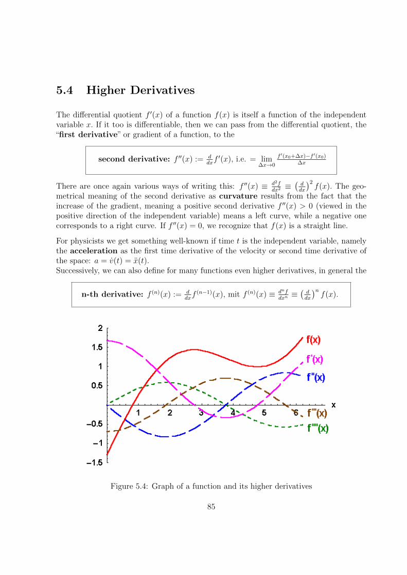
5.4 Higher Derivatives

The differential quotient f ′(x) of a function f(x) is itself a function of the independentvariable x. If it too is differentiable, then we can pass from the differential quotient, the“first derivative” or gradient of a function, to the

second derivative: f ′′(x) := ddxf ′(x), i.e. = lim

∆x→0

f ′(x0+∆x)−f ′(x0)∆x

There are once again various ways of writing this: f ′′(x) ≡ d2fdx2≡(ddx

)2f(x). The geo-

metrical meaning of the second derivative as curvature results from the fact that theincrease of the gradient, meaning a positive second derivative f ′′(x) > 0 (viewed in thepositive direction of the independent variable) means a left curve, while a negative onecorresponds to a right curve. If f ′′(x) = 0, we recognize that f(x) is a straight line.

For physicists we get something well-known if time t is the independent variable, namelythe acceleration as the first time derivative of the velocity or second time derivative ofthe space: a = v(t) = x(t).Successively, we can also define for many functions even higher derivatives, in general the

n-th derivative: f (n)(x) := ddxf (n−1)(x), mit f (n)(x) ≡ dnf

dxn≡(ddx

)nf(x).

Figure 5.4: Graph of a function and its higher derivatives

85

Insert: Extrema: From school many of you are familiar with this use of the

first and second derivative of a function from the discussion of curves:

The vanishing of the first derivative f ′(x0) = 0 at a point x0, the criterion for a

horizontal tangent in this point, is a necessary condition for the existence of a local

extremum. The condition cannot be sufficient because a horizontal turning tangent

may occur.

Sufficient conditions for a local maximum or minimum can be obtained only

by looking at the second derivative: f ′′(x0) > 0 means a turn to the left, i.e. a local

minimum, while f ′′(x0) < 0 indicates a turn to the right, thus a maximum.

Insert: Limits of Quotients: For the calculation of limits of quotients offunctions the Rule of de l’Hospital may be helpful, which states that the limit ofthe quotient of two differentiable functions is not changed by (also multiple) differ-entiation of numerator and denominator, if all concerned limits exist:

lim f(x)/g(x) = lim f ′(x)/g′(x) = lim f (n)(x)/g(n)(x)

Z.B.: limx→0

sinxx = lim

x→0

cosx1 = 1,

as was already shown geometrically in an insert of Section 4.9,

or limx→0

ex−1x = lim

x→0

ex

1 = 1,

which took us much effort to prove in Exercise 4.14d,

or limn→∞

lnxx = lim

n→∞1/x1 = 0

or limx→0

1−cosxx2

= limx→0

sinx2x = lim

x→0

cosx2 = 1/2

or limx→0

x−sinxx3

= limx→0

1−cosx3x2

= limx→0

sinx6x = lim

x→0

cosx6 = 1/6

5.5 The Technique of Differentiation

Now we can start looking at examples, applying the general definition to specific functionswhich will lead us to the rules according to which the technique of differentiation works.We shall calculate the differential quotients of all important elementary functions and putthem all together clearly in a table which will be of unexpected value for us later on.

5.5.1 Four Examples

Initially we calculate the differential quotients of four prominent examples out of ourbasic set of functions, from which we will then be able to find the derivatives of all otherinteresting functions with help of a few simple rules:

1. First of all we examine

86

the powers with natural number exponents n ∈ N : (xn)′ = nxn−1 (∗)

For the proof we use the binomial theorem:

(xn)′ = lim∆x→0

(x+ ∆x)n − xn

∆x

= lim∆x→0

xn + nxn−1∆x+ n(n− 1)xn−2(∆x)2 + ...− xn

∆x= lim

∆x→0nxn−1 + n(n− 1)xn−2∆x+ ...

= nxn−1

The n-th powers are n-times differentiable, so that xn(n) = n(n− 1)(n− 2) · . . . · 2 · 1 = n!.

2. Secondly we determine the differential quotient of

sine: (sinx)′ = cosx

The proof uses an addition theorem and a previously calculated limit:

sinx′ = lim∆x→0

sin(x+ ∆x)− sinx∆x

with help of the addition theorem

= lim∆x→0

2 sin(x+∆x−x

2

)cos(x+∆x+x

2

)∆x

= lim∆x→0

sin(

∆x2

)cos(x+ ∆x

2

)∆x2

= lim∆x→0

sin(

∆x2

)∆x2

lim∆x→0

cos

(x+

∆x

2

)= cos x.

Entirely analogously it follows for the

cosine: (cosx)′ = − sinx.

3. Finally we differentiate the

exponential function: (ex)′ = ex.

87

The proof uses a limit previously calculated in Section 4.14d:

(ex)′ = lim∆x→0

ex+∆x − ex

∆x

= ex lim∆x→0

e∆x − 1

∆x= ex

This is the characteristic property of the exponential function and the deeper reason forits outstanding importance in science, that it is identical with its own differential quotient.

Exercise 5.2 Derive the differential quotient of the cosine.

From these examples we now obtain all desired differential quotients for all functions ofour basic set and beyond, with the help of the following rules.

5.5.2 Simple Differentiation Rules: Basic Set of Functions

In practice we only very rarely have one of the four sample functions studied above todifferentiate purely on its own. Usually we have more or less complicated expressions,composed of many various functions, like for example f(x) = axne−bx(cos cx + d sin cx)with real constants a, b, c, d and n.

For this reason, we put together in this section the general rules which enable us to assem-ble the differential quotients of complicated expressions out of the well known derivativesof the individual parts. As sample applications we first of all check these rules using thefunctions of our basic set, and then beyond these further interesting functions importantfor science. We will arrange the results in a TABLE which we shall need later on alsofor integration.

In the following f(x) and g(x) are two differentiable functions and a, b, c, . . . representreal constants. You can attempt the proofs from the definition of the limit on your own,or you may have a look at the proofs in the inserts.

Due to the obvious homogeneity of the limit (a constant factor can be drawn out) (c ·f(x))′ = c · f ′(x), instead of the well-known sum rule (f(x)± g(x))′ = f ′(x)± g′(x) westart immediately with

linearity: (af(x) + bg(x))′ = a · f ′(x) + b · g′(x).

88

Here we see the differential quotient of a linear combination of functions is equal to thelinear combination of the differential quotients.

Insert: Proof:

(af(x) + bg(x))′ ≡ ( ddx)(af(x) + bg(x))

:= lim∆x→0

af(x+ ∆x) + bg(x+ ∆x)− af(x)− bg(x)

∆x

= a lim∆x→0

f(x+ ∆x)− f(x)

∆x+ b lim

∆x→0

g(x+ ∆x)− g(x)

∆x

= a( ddx)f(x) + b( d

dx)g(x) = af ′(x) + bg′(x)

With this result, the differential quotient for every polynomial e.g. of m-th degree Pm(x) =m∑n=0

anxn as a polynomial of (m− 1)-th degree follows from the power rule:

(∑m

n=0 anxn)′=∑m

n=0 ann · xn−1. Especially the (m+1)-th derivative vanishes:

P(m+1)m (x) = 0.

Many of you are familiar also with the product rule:

product rule: (f(x) · g(x))′ = f ′(x) · g(x) + f(x) · g′(x).

The differential quotient of the product of two differentiable functions f(x) and g(x) is thedifferential quotient of the first factor multiplied by the second factor, plus the differentialquotient of the second factor multiplied by the first factor:

Insert: Proof:

(f(x) · g(x))′ = ( ddx)(f(x)g(x))

:= lim∆x→0

f(x+ ∆x)g(x+ ∆x)− f(x)g(x)

∆x

= lim∆x→0

f(x+ ∆x)g(x+ ∆x)− f(x)g(x+ ∆x) + f(x)g(x+ ∆x)− f(x)g(x)

∆x

= lim∆x→0

(f(x+ ∆x)− f(x))g(x+ ∆x)

∆x+ f(x) lim

∆x→0

g(x+ ∆x)− g(x)

∆x

= ( ddx)f(x) · g(x) + f(x) · ( d

dx)g(x)

= f ′(x) · g(x) + f(x) · g′(x)

For example: (x2 sinx)′ = 2x sinx+ x2 cosx

The next rule we need is the inverse rule:

89

inverse rule:

(1

g(x)

)′= − g

′(x)g2(x)

for g(x) 6= 0.

We obtain the differential quotient of the inverse of a differentiable non-vanishing functiong(x) 6= 0 through division of the function’s differential quotient through the negative ofits square:

Insert: Proof: (1

g(x)

)′:= lim

∆x→0

1g(x+∆x) −

1g(x)

∆x

using the common denominator this gives

= lim∆x→0

g(x)− g(x+ ∆x)

g(x)g(x+ ∆x)∆x

= − lim∆x→0

g(x+ ∆x)− g(x)

∆xg(x)g(x+ ∆x)

= − g′(x)

g2(x)

This way for example, it is possible to expand the power rule onto negative exponents,meaning integers(x−n)

′= (1/xn)′ = −(xn)′/x2n = −nxn−1/x2n = −nxn−1−2n = −nx−n−1 just like above,

now however for n ∈ Z.Even the inverse exponential function can now be differentiated:(e−x)′ = −ex/(ex)2 = −e−x.

From this and linearity we obtain for the hyperbolic functions:

(sinhx)′ = ex−e−x2

′= ex+e−x

2= coshx and analogously (cosh x)′ = + sinh x.

The quotient rule follows from the product and inverse rule:

quotient rule:

(f(x)g(x)

)′=f ′(x)g(x)− f(x)g′(x)

g2(x)for g(x) 6= 0.

The differential quotient of the quotient of two differentiable functions is the differentialquotient of the numerator multiplied by the denominator function, minus the differentialquotient of the denominator multiplied by the numerator function, both divided by thesquare of the denominator function which is not allowed to vanish.

90

Insert: Proof:

(f(x)

g(x)

)′= f ′(x)

1

g(x)+

(1

g(x)

)′f(x)

=f ′(x)

g(x)− g′(x)

g2(x)f(x)

=f ′(x)g(x)− f(x)g′(x)

g2(x)

This is the way we can determine the differential quotients of all rational functions R(x) =Pn(x)Qm(x)

, i.e. the quotient of two polynomials Pn(x) and Qm(x).

We can now differentiate also tangent and cotangent:(tanx)′ = 1/ cos2 x and (cot x)′ = −1/ sin2 x,and the corresponding hyperbolic functions:(tanhx)′ = 1/ cosh2 x and (coth x)′ = −1/ sinh2 x.

Insert: Proofs: Using the quotient rule

(tanx)′ =

(sinx

cosx

)′=

cosx cosx− sinx(− sinx)

cos2 x

=cos2 x+ sin2 x

cos2 x=

1

cos2 x

(cotx)′ =

(1

tanx

)′= − 1

cos2 x tan2 x

= − 1

sin2 x

(tanhx)′ =

(sinhx

coshx

)′=

cosh2 x− sinh2 x

cosh2 x

=1

cosh2 x

(cothx)′ =

(1

tanhx

)′= − 1

cosh2 x tanh2 x

= − 1

sinh2 xfor x 6= 0.

Now we have the differential quotients of all functions in our basic set, and enter theseinto a TABLE which summarizes all of our present knowledge:

91

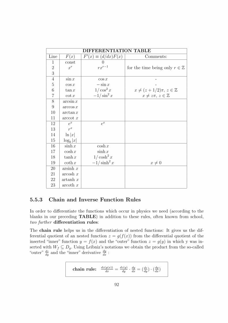
DIFFERENTIATION TABLELine F (x) F ′(x) ≡ (d/dx)F (x) Comments:

1 const 02 xr rxr−1 for the time being only r ∈ Z34 sinx cosx -5 cosx − sinx -6 tanx 1/ cos2 x x 6= (z + 1/2)π, z ∈ Z7 cotx −1/ sin2 x x 6= zπ, z ∈ Z8 arcsinx9 arccosx10 arctanx11 arccot x12 ex ex

13 rx

14 ln |x|15 logb |x|16 sinhx coshx17 coshx sinhx18 tanhx 1/ cosh2 x19 cothx −1/ sinh2 x x 6= 020 arsinh x21 arcosh x22 artanh x23 arcoth x

5.5.3 Chain and Inverse Function Rules

In order to differentiate the functions which occur in physics we need (according to theblanks in our preceding TABLE) in addition to these rules, often known from school,two further differentiation rules:

The chain rule helps us in the differentiation of nested functions: It gives us the dif-ferential quotient of an nested function z = g(f(x)) from the differential quotient of theinserted “inner” function y = f(x) and the “outer” function z = g(y) in which y was in-serted with Wf ⊆ Dg. Using Leibniz’s notations we obtain the product from the so-called“outer” dz

dyand the “inner” derivative dy

dx:

chain rule: dz(y(x))dx

= dz(y)dy· dydx

= (dzdy

) · ( dydx

)

92

in Leibniz’s and in Lagrange’s notation:

(g(f(x)))′ = g′(y)f ′(x).

Now, since we are familiar with the term differential this result may seem trivial to us,seeing how the fraction was simply reduced to higher terms by dy. Nevertheless, we wantto quickly sketch the proof to demonstrate the advantages of the differentials, with whosehelp it is very simple:

First of all for the “inner” function y = f(x) : dy = f ′(x)dx+rf with lim∆x→0

rf (x,∆x)/dx =

0, then for the “outer” function z = g(y) : dz = g′(y)dy + rg with lim∆y→0

rg(y,∆y)/dy = 0.

After insertion it follows that: dz = g′(y)(f ′(x)dx+ rf ) + rg = g′(y)f ′(x)dx+ g′(y)rf + rg,

and after division by the differential dx in the limit it becomes:

dzdx≡ ( d

dx)g(f(x)) ≡ g′(y)f ′(x) = (dg

dy)( dfdx

) ≡ (dzdy

)( dydx

).

The following example illustrates the advantages of the Leibniz notation: We are lookingfor the first derivative of ((x+ 1/x)4 − 1)3 for x 6= 0 :(

((x+ 1/x)4 − 1)3)′

= ( ddx

)w(z(y(x)))

= (dwdz

)(dzdy

)( dydx

) according to the chain rule,

= 12((x+ 1/x)4 − 1

)2(x+ 1/x)3(1− 1/x2),

since y = f(x) = x+ 1/x with ( dydx

) = 1− 1/x2,

z = g(y) = y4 − 1 with (dzdy

) = 4y3 and

w = h(z) = z3 with (dwdz

) = 3z2.

A further example is the

general exponential function: (bx)′ = bx ln b

Proof with y := x ln b : (bx)′ = ( ddx

)(ex ln b) = ( ddx

)ey = ( ddy

)ey( dydx

) = ey ln b = bx ln b.

Exercise 5.3 Chain rule:

Calculate the following differential quotients using the chain rule:a) (cosx)′ = (sin(π

2− x))′, b) (sinx2)′, c) (sin2 x)′, d) (e−x)′,

e) (exp(−x2))′ and f)(

1ax+b

)′93

Finally we need the inverse function rule for the differential quotient of the inversefunction x = f−1(y) with y ∈ Wf of a differentiable bi-unique function y = f(x) withx ∈ Df , whose differential quotient f ′(x) = dy/dx 6= 0 is known and does not vanish inthe whole Df :

inverse function rule: dxdy

= 1( dydx

)for ( dy

dx) 6= 0.

We want to derive this formula very simply in the Leibniz notation: In order to do this,we form the derivative of x = f−1(f(x)) with respect to x according to the chain rule:

1 = ( ddx

)(f−1(f(x))) = ( ddy

)(f−1(y))(df(x)dx

) = dxdy

dydx

and after division by dydx6= 0 we arrive at the stated result.

Equipped with these rules we are able now to calculate all desired derivatives. Most ofthe proofs you will find in inserts:

First of all the

roots: y = m√x = x

1m for x > 0 : m

√x ′ = (x

1m )′ = ( 1

m)x

1m−1

as inverse function of the exponential function x = ym for y > 0, for m√x ′ = (x1/m)′ =

1/(dxdy

) = 1/mym−1 = 1/m(x1/m)m−1 = (1/m)x1/m−1, i.e. our power rule (*) holds also forreciprocal integers in the exponents.

Even more generally for

rational powers: z = xnm for x > 0 : (x

nm )′ = n

mxnm−1

Meaning, our power rule (*) holds true even for any rational exponents.

Insert: Proof: with y = f(x) = x1/m in the chain rule:

(xn/m)′ = (d

dx)((x1/m)n) =

dz

dx=dz

dy· dydx

= ( ddy )yn · ( ddx)x1/m = nyn−1 · (1/m)x1/m−1

= (n/m)(x1/m)n−1x1/m−1 = (n/m)xn/m−1/m+1/m−1

= (n/m)xn/m−1

94

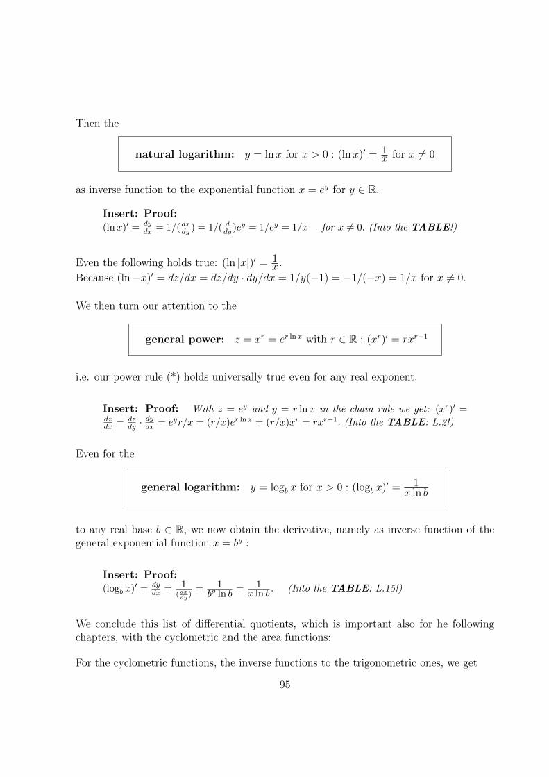
Then the

natural logarithm: y = lnx for x > 0 : (lnx)′ = 1x for x 6= 0

as inverse function to the exponential function x = ey for y ∈ R.

Insert: Proof:(lnx)′ = dy

dx = 1/(dxdy ) = 1/( ddy )ey = 1/ey = 1/x for x 6= 0. (Into the TABLE!)

Even the following holds true: (ln |x|)′ = 1x.

Because (ln−x)′ = dz/dx = dz/dy · dy/dx = 1/y(−1) = −1/(−x) = 1/x for x 6= 0.

We then turn our attention to the

general power: z = xr = er lnx with r ∈ R : (xr)′ = rxr−1

i.e. our power rule (*) holds universally true even for any real exponent.

Insert: Proof: With z = ey and y = r lnx in the chain rule we get: (xr)′ =dzdx = dz

dy ·dydx = eyr/x = (r/x)er lnx = (r/x)xr = rxr−1. (Into the TABLE: L.2!)

Even for the

general logarithm: y = logb x for x > 0 : (logb x)′ = 1x ln b

to any real base b ∈ R, we now obtain the derivative, namely as inverse function of thegeneral exponential function x = by :

Insert: Proof:(logb x)′ = dy

dx = 1( dxdy

)= 1by ln b

= 1x ln b

. (Into the TABLE: L.15!)

We conclude this list of differential quotients, which is important also for he followingchapters, with the cyclometric and the area functions:

For the cyclometric functions, the inverse functions to the trigonometric ones, we get

95

arc tangent: for −π/2 < arctanx < π/2 : (arctanx)′ = 11 + x2

Insert: Proof: With the inverse function x = tan y, where from dxdy =

1/ cos2 y = (cos2 y + sin2 y)/ cos2 y = 1 + tan2 y = 1 + x2 follows: (arctanx)′ =dydx = 1/(dxdy ) = 1/(1 + x2). (Into the TABLE: L.10!)

Analogously for the

arc cotangent for 0 < arccot x < π : (arccot x)′ = − 11 + x2

Exercise 5.4 Prove this with the inverse function: x = cot y.

For the

arc cosine for −π/2 < arcsinx < π/2 : (arcsinx)′ = 1√1− x2

for |x| < 1

Insert: Proof: With the inverse function x = sin y, where from dxdy = cos y =√

(1− sin2 y) =√

(1− x2) for |x| < 1 follows: (arcsinx)′ = dydx = 1/(dxdy ) =

1/√

(1− x2). (Into the TABLE: L.8!)

Analogously for

arc cosine for 0 < arccosx < π : (arccosx)′ = − 1√(1− x2)

for |x| < 1

Exercise 5.5 Prove this with the inverse function: x = cos y.

The area functions the inverse functions of the hyperbolic functions, complete our dif-ferentiation table:

For the

96

area hyperbolic tangent: (artanh x)′ = 11− x2 for |x| < 1

and the

area hyperbolic cotangent: (arcoth x)′ = − 1x2 − 1

for |x| > 1.

Exercise 5.6 Prove this with the inverse function: x = tanh y, respectively with x =coth y.

For the

area hyperbolic sine: (arsinh x)′ = 1√(1 + x2)

for x ∈ R.

and

area hyperbolic cosine: 0 < arcosh x :

(arcosh x)′ = 1√(x2 − 1)

for x ≥ 1.

Exercise 5.7 Prove this with the inverse function: x = sinh y, respectively with x =cosh y ≥ 1, bi-unique only for y > 0.

You will find all the preceding results combined below results in the big differentiationtable, to which we will return very often later on:

97

DIFFERENTIATION TABLELine F (x) F ′(x) ≡ (d/dx)F (x) Comments:

1 const 02 xr rxr−1 r ∈ R34 sinx cosx5 cosx − sinx6 tanx 1/ cos2 x x 6= (z + 1/2)π, z ∈ Z7 cotx −1/ sin2 x x 6= zπ, z ∈ Z8 −π/2 < arcsinx < π/2 1/

√(1− x2) |x| < 1

9 0 < arccosx < π −1/√

(1− x2) |x| < 110 −π/2 < arctanx < π/2 1/(1 + x2)11 0 < arccot x < π −1/(1 + x2)12 ex ex

13 rx rx ln r 0 < r ∈ R14 ln |x| 1/x x 6= 015 logb |x| 1/x ln b x 6= 0, 0 < b ∈ R, b 6= 116 sinhx coshx17 coshx sinhx18 tanhx 1/ cosh2 x19 coth x −1/ sinh2 x x 6= 0

20 arsinh x 1/√

(x2 + 1)

21 0 < arcosh x 1/√

(x2 − 1) x > 122 artanh x 1/(1− x2) |x| < 123 arcoth x −1/(x2 − 1) |x| > 1

Exercise 5.8 Differentiation examples

Determine the differential quotients for the following functions y = f(x) with constantsa, b, c and d:a) y = sin3(4x), b) y = exp(−(x/a)2), c) y = 1√

ax2+b, d) y = ln(3e2x),

e) y = a cosh x−ba

, f) y = ax2 exp(−bx), g) y = cos(ax+ b) sin(cx+ d),

h) y = 11+(x/a)2

, i) y =(

sin(x/a)(x/a)

)2

, j) y = arctan(1/x) + (x/2) (lnx2 − ln(x2 + 1))

Calculate the first five derivatives of the following functions f(x) which we will need inthe next chapter:k) f(x) = sinx, l) f(x) = tan x, m) f(x) = ex and n) f(x) = 1

1−x2

98

5.6 Numerical Differentiation

In some cases we cannot or do not want to calculate the derivative of a function analyticallyaccording to the rules from the last section. This is the case for example when we do notknow an analytical form for the graph of a function. Then we have to rely on numericaldifferentiation.

Our definition formula of the differential quotient from Section 5.2:

f ′(x0) = lim∆x→0

f(x0 + ∆x)− f(x0)

∆x

can also be used for the numerical calculation of the derivative. For the point (x0, f(x0)),we look for neighbouring points (x0 + ∆x, f(x0 + ∆x)), calculate the difference quotientand let ∆x tend to 0.

Since computer numbers are stored only with a certain accuracy (for example with 8decimal places), rounding errors occur in forming the differences f(x0+∆x)−f(x0) which,even though these rounding errors always remain of the same order, increase relative tothe value of the difference more and more. Thus the difference quotient approximatesf ′(x0) increasingly accurately with decreasing ∆x, but eventually the deviation begins todominate with decreasing ∆x due to the numerical roundings. Therefore, we must cometo a compromise. We find a better approximation if

f ′(x0) = lim∆x→0

f(x0 + ∆x)− f(x0 −∆x)

2∆x

With the help of the Taylor series (which we will examine in the next chapter) we canshow that the error is reduced through the symmetrization of ∆xf ′′(x0)/2! to the orderof (∆x)2f ′′′(x0)/3!. Thus the error becomes smaller with ∆x quadratically.

5.7 Preview of Differential Equations

To motivate you for this chapter about differentiation we mentioned at the outset thatmany laws of nature can be expressed in the form of differential equations. What aredifferential equations?

A differential equation is a relation between a function f(x) of interest and itsdifferential quotients f ′(x), f ′′(x), . . .

When e.g. we fasten a weight to a spiral spring hanging down from the ceiling and call theamount by which the spring is stretched x(t), where t means the time, Newton’s secondNewtonian law yields, if we neglect air resistance, the following differential equation:

x(t) + ω2x(t) = 0 with a constant ω.

99

Like most of the differential equations of physics this one is of “second order”, i.e. thehighest occurring differential quotient is the second derivative of the desired function.While in a “normal” equation for one unknown variable, for instance x2 − 1 = 0, thenumerical solutions x, like x = ±1 are the goal, in the differential equation above functionsof the time variable x(t) are what one seeks. We can easily see that x(t) = sinωt is asolution, since x(t) = ω cosωt and consequently x(t) = −ω2 sinωt. But is this the onlysolution? You surely will be dealing very extensively with questions of this kind.

Exercise 5.9 Physical differentiation

Determine the first x(t) derivative and second x(t) derivative of the following functionsx(t) of time t with the constants x0, v0, g, ω, ω0, γ, ρ, b0, w, m0 and µ:The comparison of x(t) with combinations of x(t) and x(t) will lead you to “differentialequations”. Do you recognize the physical systems described by these differential equations?What is the physical meaning of the constants involved?a) x(t) = x0 + v0t

b) x(t) = x0 + v0t− gt2/2c) x(t) = x0 cosωt+ v0

ωsinωt

d) x(t) = x0 + v0ρ

(1− e−ρt)

e) x(t) = x0 − gtρ

+ v0+g/ρρ

(1− e−ρt)

f) x(t) = −1r

ln cosh(t√gr)

g) x(t) = x0 cosh γt+ (v0/γ) sinh γt

h) x(t) = e−ρt(x0 cos t

√ω2 − ρ2 + v0+ρx0√

ω2−ρ2sin t

√ω2 − ρ2

)i) x(t) = e−ρt

(x0 cosh t

√ρ2 − ω2 + v0+ρx0√

ρ2−ω2sinh t

√ρ2 − ω2

)j) x(t) = b0√

(ω20−ω2)2+4ω2ρ2

cos(ωt− arctan 2ωρ

ω20−ω2

)k) x(t) = x0 tanh(ωt)

l) x(t) = wm0

µ(1− µt

m0) ln(1− µt

m0)− gt2/2 + wt

Later on, in treating functions of several variables you will meet even more complicateddifferential operations: with help of the so-called “partial” derivatives you will form gra-dients of scalar fields as well as the divergence or rotation of vector fields. Whenever thecalculation of numbers is concerned, you will need nothing else than what we have learnedhere.

100

Exercise 5.10 Partial derivatives

The change of functions of several variables, for instance fields of the three position vari-ables x1, x2, x3, you will later describe through so-called partial differential quotients, inwhich only one of the variables , e.g. x1, is changed and all others are fixed: in this casex2 = const and x3 = const. Without any further insight into the deeper background of the“partial” derivatives (for which a new notation Nabla: 51 must be introduced) given thethings learned above you are already now able to calculate these “partial” derivatives. Todo this you handle the fixed variables exactly as you do physical constants. Calculate forinstance:

a) ddx1

(x1 + x2 + x3) b) ddx1

(x21 + x2

2 + x23) c) d

dx1(x1x2x3)

d) limx1→0

ddx1

(2x1x2

x21 + x2

2

)and e) d

dx1

1√x2

1 + x22 + x2

3

101

Chapter 6

TAYLOR SERIES

Here we want to examine one of the principal applications of differential calculus, andthis rather closely. Because far too little time is spent on this subject in schools, eventhough this technology is vital to natural scientists. We are going to talk about Taylorseries which allow us to represent and calculate a large number of functions f(x) neededin physics, in the neighbourhood of some value x0 of the independent variable x, in termsof a power series.

6.1 Power Series

By far the simplest functions are the powers xn with natural number exponents n ∈ N,

and the polynomials Pm(x) =m∑n=0

anxn formed through addition and multiplication of

those, whose function values can quickly be calculated. Also the infinite power series∞∑n=0

anxn, being limits of polynomial partial sums, are relatively easy as long as the are

absolutely convergent, compared to the huge variety of elementary functions studied byus. Power series can be added or subtracted and absolutely convergent ones can alsobe multiplied, divided and even differentiated term by term (and integrated as we willdiscover later). It would be great if we only needed to concern ourselves with such powerseries!

We shall see, this dream can become reality to a certain extent. Differential quotients arethe key to this eldorado.

103

6.2 Geometric Series as Model

First of all let us examine once again the simplest of all polynomials, the geometric

sum Gm(x) :=m∑n=0

xn with coefficients an = 1 for all non-negative integers n and the

accompanying powers series, the geometric series:

geometric series: G∞(x) :=∞∑n=0

xn = 1 + x+ x2 + x3 + x4 + ...

=1

1− xfor |x| < 1

Here we already have a prototype for our dream: the rational function 1/(1−x) is displayedin the open interval ] − 1, 1[ around the point x0 = 0 in terms of a power series, namely

the geometric series∞∑n=0

xn, meaning it is approximated by the sum of the constant “one”,

the bisector line of the first and third sector, the standard parabola, a function of thirddegree, and so on. Admittedly this series has an infinite number of terms, but it canbe calculated using only multiplication and addition, and depending on the demand foraccuracy, a few terms may be already sufficient. This representation however only existsin the interval ]− 1, 1[, while the function 1/(1− x) is defined everywhere other than forx = 1.

This example encourages us to ask the following questions:

1. Are there power series also for other functions which can represent these functionsin certain intervals?

2. How can we obtain the coefficients in the series an ?

3. How many different series exist for a function?

4. How good is the convergence, respectively how large is the approximation error, ifwe break off the series?

6.3 Form and Non-ambiguity

Before we deal with the question of existence, we want to turn our attention to thequestions 2 and 3: In order to get information about the characteristics of the desired

104

series, we want to assume for the time being, that we already have found a suitable powerseries:

f(x) =∞∑n=0

anxn = a0 + a1x+ a2x

2 + a3x3 + a4x

4 + ...

with f(0) = a0 which represents the function f(x) of interest in an interval, e.g. for |x| < Raround the origin. Since all functions of our basic set are infinitely times differentiable,we are able to calculate the derivatives of the power series one after another:

f ′(x) =∞∑n=1

nanxn−1 = a1 + 2a2x+ 3a3x

2 + 4a4x3 + . . .

with f ′(0) = a1, thus a1 =f ′(0)

1!

f ′′(x) =∞∑n=2

n(n− 1)anxn−2 = 2a2 + 3 · 2a3x+ 4 · 3a4x

2 + . . .

with f ′′(0) = 2a2, thus a2 =f ′′(0)

2!

f ′′′(x) =∞∑n=3

n(n− 1)(n− 2)anxn−3 = 3!a3 + 4!a4x+ . . .

with f ′′′(0) = 3! a3, thus a3 =f ′′′(0)

3!

In general:

f (n)(x) = n! an + (n+ 1)! an+1x+ (n+ 2)!an+2x2 + . . .

with f (n)(0) = n! an, thus an =f (n)(0)

n!.

In this way we find the desired coefficients an from the derivatives f (n)(0) of the function,evaluated at the expansion point x0 = 0, to be represented. If then a power seriesrepresentation of our function exists, it has the following form and we call it:

TAYLOR SERIES: f(x) =∞∑n=0

f (n)(0)n!

xn

According to the given construction the coefficients are in addition unambiguous, sothat we have answered question 3, too.

105

Our calculations also show us that the function to be represented necessarily mustbe infinitely times differentiable for the Taylor series to exist. That the necessaryprecondition is not sufficient for the existence of a Taylor series is shown through thefollowing counter example: The function f(x) = exp(−1/x2) for x 6= 0 and f(0) = 0.Although this function is infinitely times differentiable, all its derivatives f (n)(0) = 0vanish at the point x = 0, so that no Taylor series around 0 can be constructed.

Figure 6.1: Graph of the function f(x) = exp(−1/x2) for x 6= 0 and f(0) = 0

Exercise 6.1 As a consistency test, calculate the Taylor series of our model, the geomet-ric series for |x| < 1.

Figure 6.2: The geometric series as a Taylor series of the rational function

106

6.4 Examples from the Basic Set of Functions

First of all we consider some examples from our basic set of functions:

6.4.1 Rational Functions

The functions xn with natural number exponents n ∈ N are special cases of power serieswith one single term only. Powers of x with negative exponents are not at all defined forx = 0.

However, the general binomial series with real exponents r ∈ R can be developed:

f(x) = (1 + x)r =∞∑n=0

(rn

)xn = 1 + r

1!x+

r(r − 1)2!

x2 +r(r − 1)(r − 2)

3!x3 + . . .

with the generalized binomial coefficient(rn

):= r(r−1)(r−2)...(r−n+1)

n!and

(r0

):= 1.

As proof:

f ′(x) = r(1 + x)r−1, f ′′(x) = r(r − 1)(1 + x)r−2,

f ′′′(x) = r(r − 1)(r − 2)(1 + x)r−3, . . . etc.

generally f (n)(x) = r(r − 1)(r − 2) . . . (r − n+ 1)(1 + x)r−n

with f(0) = 1, f ′(0) = r,

f ′′(0) = r(r − 1), f ′′′(0) = r(r − 1)(r − 2), . . . etc.

generally f (n)(0) = r(r − 1)...(r − n+ 1)

altogether:(1 + x)r = 1 +

r

1!x+

r(r − 1)

2!x2 +

r(r − 1)(r − 2)

3!x3 + . . .

= 1 +∞∑n=1

r(r − 1)(r − 2)...(r − n+ 1)/n! · xn =∞∑n=0

(r

n

)xn.

Some special cases are of particular importance:

First we recover for natural r = n ∈ N our previously derived binomial formula for thespecial case a = 1 and b = x, since the power series breaks off in case of natural numberexponents:

(1 + x)n =m∑n=0

(m

n

)xn

For negative r ∈ Z, e.g. for r = −1 the alternating geometric series results once more

107

1

(1 + x)= 1− x+ x2 − x3 ± . . . =

∞∑n=0

(−1)nxn,

and for r = −2 its negative derivative:

1

(1 + x)2= 1− 2x+ 3x2 − 4x3 ± . . . =

∞∑n=0

(−1)n(n+ 1)xn.

For fractional r ∈ Q, e.g. r = 1/2 or −1/2 we get the frequently needed series of thesquare root in the numerator or denominator

√1 + x = 1 + (1/2)x− (1/8)x2 + (1/16)x3 − (5/128)x4 ± . . . resp.

1/√

(1 + x) = 1− (1/2)x+ (3/8)x2 − (5/16)x3 + (35/128)x4 ∓ . . .

Exercise 6.2 Calculate the Taylor series of (1 + x)r for r = −3, 1/3 and −1/3.


As the next example we chose one of the trigonometric functions, namely the sine:

f(x) = sinx =∞∑n=0

(−1)nx2n+1/(2n+ 1)! = x− x3/3! + x5/5!− x7/7!± . . .

As proof: f ′(x) = cos x, f ′′(x) = − sinx,

f ′′′(x) = − cosx, f (4)(x) = sin x, . . .

with f(0) = 0, f ′(0) = 1,

f ′′(0) = 0, f ′′′(0) = −1,

f (4)(0) = 0, . . .

altogether: sin x =∞∑n=0

(−1)nx2n+1/(2n+ 1)!

Insert: : From this we see once more that

limx→0

sinx

x= lim

x→0

x− x3/ 3! + x5/ 5!∓ . . .x

= limx→0

(1− x2/ 3! + x4/ 5!∓ . . .) = 1

what we earlier have proved according to de l’Hospital.

108

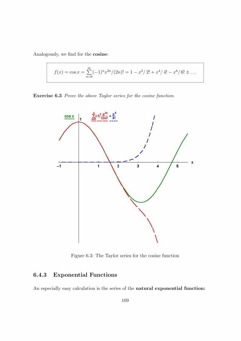
Analogously, we find for the cosine:

f(x) = cos x =∞∑n=0

(−1)nx2n/(2n)! = 1− x2/ 2! + x4/ 4!− x6/ 6!± . . .

Exercise 6.3 Prove the above Taylor series for the cosine function.

Figure 6.3: The Taylor series for the cosine function

6.4.3 Exponential Functions

An especially easy calculation is the series of the natural exponential function:

109

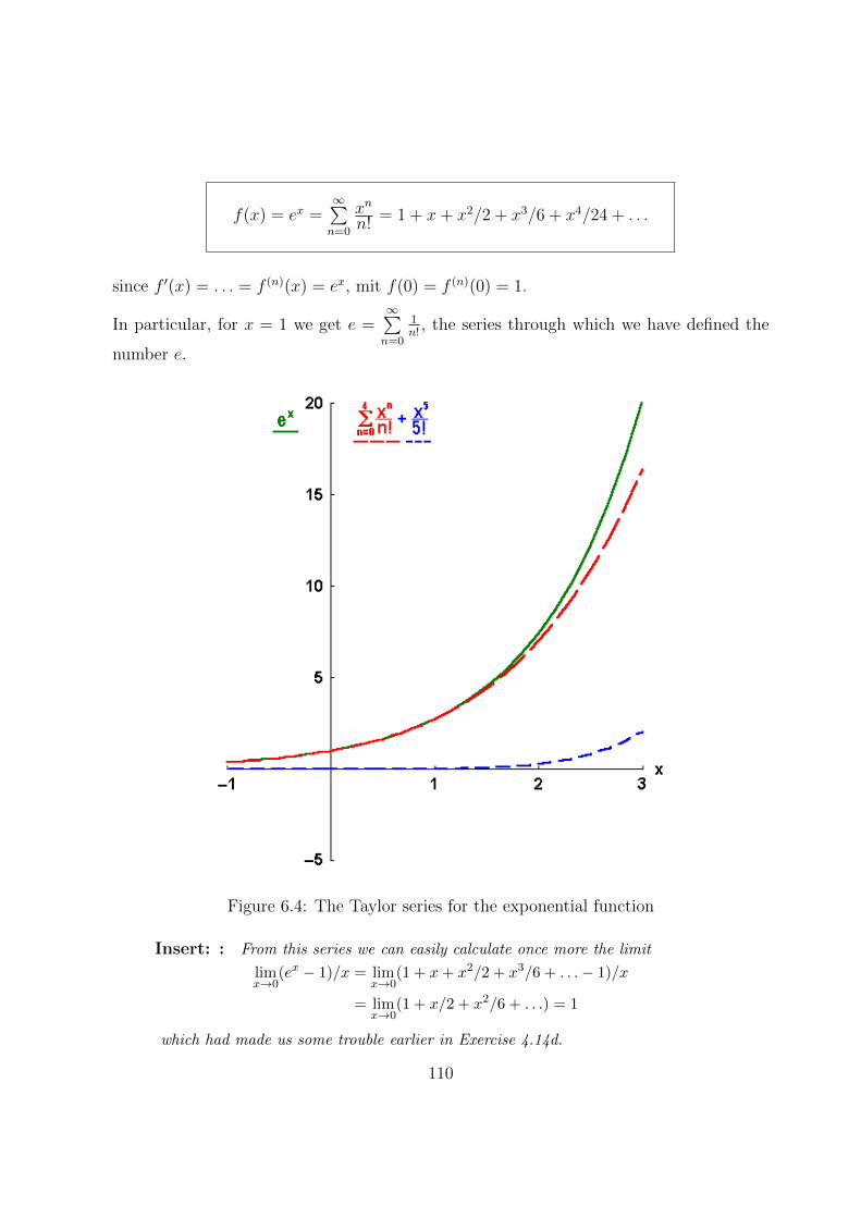
f(x) = ex =∞∑n=0

xn

n!= 1 + x+ x2/2 + x3/6 + x4/24 + . . .

since f ′(x) = . . . = f (n)(x) = ex, mit f(0) = f (n)(0) = 1.

In particular, for x = 1 we get e =∞∑n=0

1n!, the series through which we have defined the

number e.

Figure 6.4: The Taylor series for the exponential function

Insert: : From this series we can easily calculate once more the limit

limx→0

(ex − 1)/x = limx→0

(1 + x+ x2/2 + x3/6 + . . .− 1)/x

= limx→0

(1 + x/2 + x2/6 + . . .) = 1

which had made us some trouble earlier in Exercise 4.14d.

110

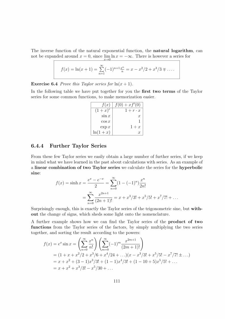
The inverse function of the natural exponential function, the natural logarithm, cannot be expanded around x = 0, since lim

x→0lnx = −∞. There is however a series for

f(x) = ln(x+ 1) =∞∑n=1

(−1)n+1 xn

n= x− x2/2 + x3/3∓ . . . .

Exercise 6.4 Prove this Taylor series for ln(x+ 1).

In the following table we have put together for you the first two terms of the Taylorseries for some common functions, to make memorization easier.

f(x) f(0) + xf ′(0)(1 + x)r 1 + r · x

sinx xcosx 1expx 1 + x

ln(1 + x) x

6.4.4 Further Taylor Series

From these few Taylor series we easily obtain a large number of further series, if we keepin mind what we have learned in the past about calculations with series. As an example ofa linear combination of two Taylor series we calculate the series for the hyperbolicsine:

f(x) = sinh x =ex − e−x

2=∞∑n=0

(1− (−1)n)xn

2n!

=∞∑n=0

x2n+1

(2n+ 1)!= x+ x3/3! + x5/5! + x7/7! + . . .

Surprisingly enough, this is exactly the Taylor series of the trigonometric sine, but with-out the change of signs, which sheds some light onto the nomenclature.

A further example shows how we can find the Taylor series of the product of twofunctions from the Taylor series of the factors, by simply multiplying the two seriestogether, and sorting the result according to the powers:

f(x) = ex sinx =

(∞∑n=0

xn

n!

)(∞∑m=0

(−1)mx2m+1

(2m+ 1)!

)= (1 + x+ x2/2 + x3/6 + x4/24 + . . .)(x− x3/3! + x5/5!− x7/7!± . . .)= x+ x2 + (3− 1)x3/3! + (1− 1)x4/3! + (1− 10 + 5)x5/5! + . . .

= x+ x2 + x3/3!− x5/30 + . . .

111

Even with nested functions, whose Taylor series of inner and outer functions are known tous, it is often easier to insert these in each other than to directly calculate the differentialquotients: For instance

f(x) = exp(sin x) =∞∑n=0

(∞∑m=0

(−1)mx2m+1

(2m+ 1)!

)n

/n!

= 1 + (x− x3/3! + . . .) + (x− x3/3! + . . .)2/2 + (x− x3/3! + . . .)3/3! + . . .

= 1 + x+ x2/2 + (1− 1)x3/3! + (1− 4)x4/4! + . . .

= 1 + x+ x2/2− x4/8 + . . .

Exercise 6.5 Calculate the Taylor series of the following functions

a) the hyperbolic cosine: coshx,b) the bell-shaped Gauss function : exp(−x2),c) of 1/(1− x)2 through termwise differentiation of the geometric series.

Exercise 6.6 Calculate the first four terms of the Taylor series

a) of tanx through division of the seriesb) of the product ex sinx directly trough calculation of the derivativesc) of the nested function exp(sinx) likewise directly.

6.5 Convergence Radius

Already with our model, the geometric series, the validity of the series development waslimited to the interval |x| < 1 around the origin. Also for the other Taylor series, evenif the function to be represented is infinitely often differentiable in a closed interval (i.e.including the boundary points), the convergence is generally limited to the inner of aninterval symmetrical about the origin: |x| < R. The number R is called “convergenceradius”. The term “radius”, however, is understandable only in the theory of functions,i.e. with power series of complex numbers. Within this symmetrical convergence regionlimited by R, all Taylor Series converge absolutely. Outside, i.e. for |x| > R, they aredivergent. The convergence at both the boundary points must be examined separately inevery individual case. Mathematicians provide us (through comparison with for examplethe geometric series) with methods for determining the convergence radius.

We would like to report here only one of these sufficient conditions for the absolute

convergence of a series f(x) =∞∑n=0

anxn, namely D’Alembert’s quotient-criterion,

using which the radius can be written as follows:

112

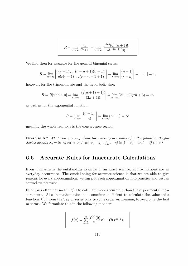
R = limn→∞

∣∣∣ anan+1

∣∣∣ = limn→∞

∣∣∣∣f (n)(0) (n+ 1)!

n! f (n+1)(0)

∣∣∣∣ .We find then for example for the general binomial series:

R = limn→∞

∣∣∣∣r(r − 1) . . . (r − n+ 1)(n+ 1)!

n!r(r − 1) . . . (r − n− 1 + 1)

∣∣∣∣ = limn→∞

∣∣∣∣(n+ 1)

(r − n)

∣∣∣∣ = | − 1| = 1,

however, for the trigonometric and the hyperbolic sine:

R = R[sinhx; 0] = limn→∞

∣∣∣∣(2(n+ 1) + 1)!

(2n+ 1)!

∣∣∣∣ = limn→∞

(2n+ 2)(2n+ 3) =∞

as well as for the exponential function:

R = limn→∞

∣∣∣∣(n+ 1)!

n!

∣∣∣∣ = limn→∞

(n+ 1) =∞

meaning the whole real axis is the convergence region.

Exercise 6.7 What can you say about the convergence radius for the following TaylorSeries around x0 = 0: a) cosx and coshx, b) 1

1−3x, c) ln(1 + x) and d) tanx?

6.6 Accurate Rules for Inaccurate Calculations

Even if physics is the outstanding example of an exact science, approximations are aneveryday occurrence. The crucial thing for accurate science is that we are able to givereasons for every approximation, we can put each approximation into practice and we cancontrol its precision.

In physics often not meaningful to calculate more accurately than the experimental mea-surements. Also in mathematics it is sometimes sufficient to calculate the values of afunction f(x) from the Taylor series only to some order m, meaning to keep only the firstm terms. We formulate this in the following manner:

f(x) =m∑n=0

f (n)(0)n!

xn +O(xm+1).

113

Here O(xm+1) means that the neglected terms are at least of order xm+1 , i.e. they containm+ 1 or more factors x.

In this section we want to put together the rules for doing approximate calculations. Inthis case the approximation consists in consistently taking into account all terms up tothe order xm. Which rules follow from this recipe can be displayed most easily for thefrequent case m = 1, i.e. the series is broken off already after the second term:

f(x) = f(0) + x · f ′(0) +O(x2) = f0 + x · f ′0 +O(x2)

with the following abbreviations f0 = f(0) and f ′0 = f ′(0).

We consider a second function with analogous notations:

g(x) = g0 + x · g′0 +O(x2).

Please realize that we use the same term O(x2) in the series for both f(x) and g(x): O(x2)stands not for a certain numerical value, but is only a symbolic way of writing what hasbeen omitted.

For the product of the two functions f(x) and g(x) we get then:

f(x) · g(x) = f0g0 + x(f ′0g0 + f0g′0) + x2f ′0g

′0 + (f0 + x · f ′0 + g0 + x · g′0)O(x2)

Here the first three terms are well defined, in the last term however concrete terms aremultiplied with the symbol O(x2). What does this mean?

We may write O(x2) =m∑n=2

anxn with some coefficients an. Then the first part of the term

of interest can be written

f0O(x2) =m∑n=2

(f0an)xn =m∑n=2

bnxn = O(x2),

since this series starts again with x2, although with the coefficients bn = f0an. Further-more:

xf ′0O(x2) =m∑n=2

(f ′0an)xn+1 =m∑n=3

cnxn = O(x3),

because this series starts with a term proportional to x3. For the sum we get

(f0 + xf ′0)O(x2) = O(x2) +O(x3) = O(x2),

since the lowest (and in the neighbourhood of the origin dominant) power is x2. If weidentify also the third term in the expression for the product f(x)g(x) as of the order x2

and add it to the rest, we receive altogether:

114

f(x) · g(x) = f0g0 + x(f ′0g0 + f0g′0) +O(x2).

We would have gotten also the same expression if we had calculated the Taylor series forthe product function F (x) := f(x)g(x)

F (x) = F (0) + xF ′(0) +O(x2),

where F (0) = f0g0 and the product rule of differentiation would have lead us to F ′(0) =f ′0g0 + f0g

′0. One additional warning : Over-eager people might think that we should have

included in the approximate expression for f(x)g(x) at least the term x2f ′0g′0 which could

have easily been calculated. That would however be inconsistent, since other terms ofthe same order have been neglected.

For the r-th power of an arbitrary function f(x) we get:

f r(x) = f r0 (1 + xf ′0f0

)r = f r0 (1 + rxf ′0f0

) +O(x2)

where we have taken the binomial series (1+x)r = 1+r ·x+O(x2) from our small table.Especially for r = −1, i.e. the inverse of a function f(x) follows:

f−1(x) = f−10 (1− xf

′0

f0) +O(x2).

We find the same expression clearly also if we break off the Taylor series for the inversefunction after the second term.

For nested functions F (x) = f(g(x)) we use most simply the Taylor series directly,

f(g(x)) = f(g(0)) + xf ′(g(0)) g′(0) +O(x2).

As a numerical example let us consider the problem of calculating (1.2)1/20 = (1 +0.2)1/20 = 1 + 0.2/20 + O((0.2)2) = 1.01 + O(0.04), while the exact value is 1.00915and the error lies near 0.0008.

Exercise 6.8 Develop around the point x = 0 up to first order:

a) (1 + x)ex, b) e−x sinx, c) 3√

8 + x, d) sinx cosx, e) 1coshx

and f) exp(sinx)

Exercise 6.9 Calculate up to first order and compare with the exact values:

a) sin 0.1, b) e−0.3, c) ln 0.8 = ln(1− 0.2) and d) 171/4 = (16 + 1)1/4

115

6.7 Quality of Convergence: the Remainder Term

After the results of the last sections, only question 4) about the quality of convergenceremains unanswered: Even if we are sure of the convergence of the series, it is clearlyessential to know how large the error would be when we use only an

approximation polynomial of m-th degree: Pm(x) =m∑n=0

f (n)(0)n!

xn instead of the

entire infinite power series.

Instead of the exact calculation of the

remainder term rm(x) := f(x)− Pm(x),

we shall only report here the formula which results from this calculation and can serve toestimate rm(x), the so-called

Lagrange form of the remainder term rm(x) =f(m+ 1)(θx)

(m+ 1)!xm+1, where 0 < θ < 1.

At first sight this expression seems a bit astonishing, since it is expressed in terms ofthe (m + 1)-th term of the series, i.e. the first neglected term. This remainder termshould, however, replace the whole remainder of the series. The apparent contradictionis resolved by the observation that the (m+ 1)-th derivative in the remainder term is notto be evaluated at the point of development 0, but rather at a unknown intermediatepoint θx in between the expansion point 0 and the point of interest x, expressed by theunknown number θ with 0 < θ < 1. Because of the fact that θ is unknown, the remainderterm can generally not be calculated, but must be

estimated: |rm(x)| ≤ max0<θ<1

|f (m+1)(θx)||xm+1|(m+1)!

.

From this estimate formula we can see that the error decreases as the (m + 1)-th powerof the distance from the point x to the expansion point 0. Thus it is favorable to go asnear to the expansion point as possible.

116

As an example we calculate sin 100 = sin(5π/9) up to r5(x) with help of the Taylor seriesaround the point x0 = 0, obtained in Section 6.4.2

sinx = x− x3/3! + x5/5!− r5(x) :

We get: sin(5π/9) = 0.9942 − r5(5π/9), where the estimate of the remainder term withθ = 0 yields:

|r5(5π/9)| ≤ (5π/9)7/7! = 0.0098.

The correct value is 0.98480... differing from the approximation value by 0.0094.

Exercise 6.10 Calculate the quadratic terms of the Taylor series and the remainderterms r2(x) in our small table from Section 6.4.3. Choose e.g. r = 1/2, −1/2 and−1 and estimate the errors: At what points x do the relative errors r2(x)/f amount to1% or 10%, respectively?

Exercise 6.11 Calculate4√e3 with the Taylor series around x0 = 0 up to r3.

6.8 Taylor Series around an Arbitrary Point

In the last section we have seen how much depends on the proximity to the expansionpoint of development in the application of the Taylor series, when calculating to calculatefunction values in the neighbourhood of expansion points for which the function is wellknown. Therefore, we finally turn to the problem of optimizing the expansion point x0

which till now we always have chosen to be 0.

We obtain the general Taylor series around any point x0 from our present form verysimply by replacing x everywhere by y := x− x0 and expanding the resulting function ofy in the neighborhood of y = 0. Thus we get for infinitely often differentiable functionsf(x) the form of the general

Taylor series around the point x0 : f(x) =∞∑n=0

f (n)(x0)n!

(x− x0)n,

for the convergence radius R the sufficient quotient criterion:

R = limn→∞

∣∣∣ anan+1

∣∣∣ = limn→∞

∣∣∣f (n)(x0) (n+1)fn+1(x0)

∣∣∣117

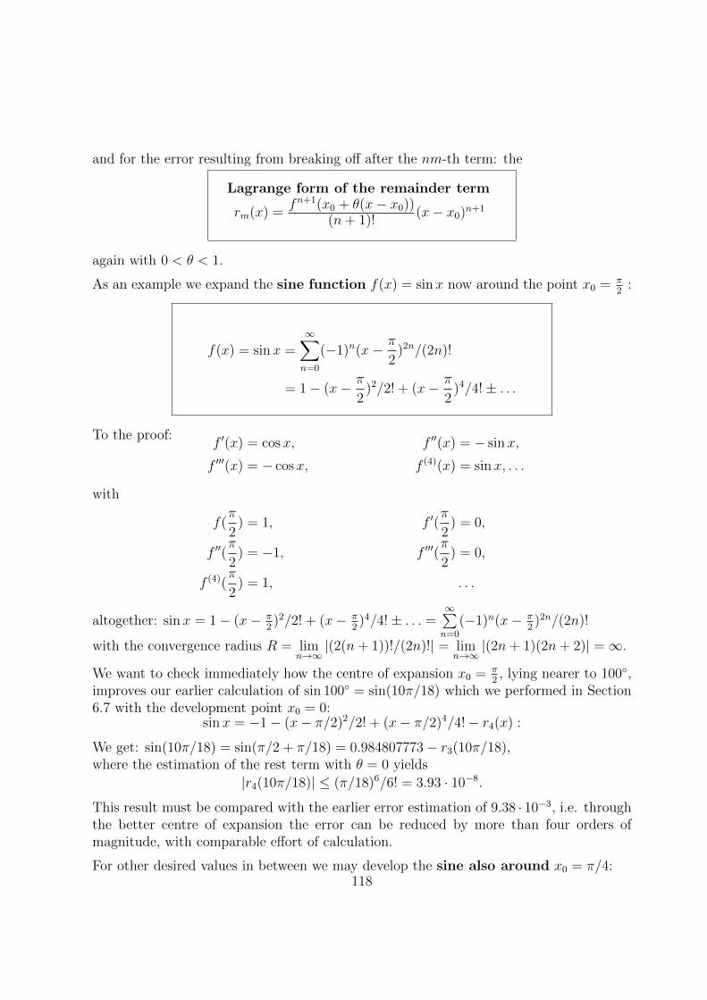
and for the error resulting from breaking off after the nm-th term: the

Lagrange form of the remainder term

rm(x) =fn+1(x0 + θ(x− x0))

(n+ 1)!(x− x0)n+1

again with 0 < θ < 1.

As an example we expand the sine function f(x) = sin x now around the point x0 = π2

:

f(x) = sinx =∞∑n=0

(−1)n(x− π

2)2n/(2n)!

= 1− (x− π

2)2/2! + (x− π

2)4/4!± . . .

To the proof:f ′(x) = cos x, f ′′(x) = − sinx,

f ′′′(x) = − cosx, f (4)(x) = sinx, . . .

with

f(π

2) = 1, f ′(

π

2) = 0,

f ′′(π

2) = −1, f ′′′(

π

2) = 0,

f (4)(π

2) = 1, . . .

altogether: sin x = 1− (x− π2)2/2! + (x− π

2)4/4!± . . . =

∞∑n=0

(−1)n(x− π2)2n/(2n)!

with the convergence radius R = limn→∞

|(2(n+ 1))!/(2n)!| = limn→∞

|(2n+ 1)(2n+ 2)| =∞.

We want to check immediately how the centre of expansion x0 = π2, lying nearer to 100,

improves our earlier calculation of sin 100 = sin(10π/18) which we performed in Section6.7 with the development point x0 = 0:

sinx = −1− (x− π/2)2/2! + (x− π/2)4/4!− r4(x) :

We get: sin(10π/18) = sin(π/2 + π/18) = 0.984807773− r3(10π/18),where the estimation of the rest term with θ = 0 yields

|r4(10π/18)| ≤ (π/18)6/6! = 3.93 · 10−8.

This result must be compared with the earlier error estimation of 9.38 · 10−3, i.e. throughthe better centre of expansion the error can be reduced by more than four orders ofmagnitude, with comparable effort of calculation.

For other desired values in between we may develop the sine also around x0 = π/4:118

f(x) = sinx = (1/√

2)[1 + (x− π/4)− (x− π/4)2/2!− (x− π/4)3/3! + +−− . . .]

since f ′(x) = cos x, f ′′(x) = − sinx, f ′′′(x) = − cosx, f (4)(x) = sinx, . . .with f(π/4) = 1/

√2, f ′(π/4) = 1/

√2, f ′′(π/4) = −1/

√2, f ′′′(π/4) = −1/

√2, f (4)(π/4) =

1/√

2,altogether: sin x = (1/

√2)[1 + (x− π/4)− (x− π/4)2/2!− (x− π/4)3/3! + +−− . . .

with the convergence radius R = limn→∞

|(n+ 1)!/n!| = limn→∞

|n+ 1| =∞.

Now we are able to present a series also for the natural logarithm, e.g. around x0 = 1 :

f(x) = ln x =∞∑n=1

(−1)n+1(x− 1)n/n = (x− 1)− (x− 1)2/2 + (x− 1)3/3 + . . .

If we replace here x by x + 1, we arrive again at our earlier Taylor series for ln(x + 1)around the point 0.

Exercise 6.12 Determine the Taylor series and the convergence regions for:

1) sinx around point x0 = π,2) ex around point x0 = 1,3) ex around point x0 = 2 and4) prove the series for lnx around the point x0 = 1 given above.

Exercise 6.13 Calculate once more4√e3 up to r3, but now using the Taylor series around

x0 = 1 and compare with our earlier calculation around x0 = 0 in Exercise 6.11.

You will get to know and carry out many more series expansions during your studies.There are expansion series also for fields, for instance the famous multipole series. Youwill expand the frequently used periodic functions “after Fourier in the quadratic mean”with cosine and sine as basis functions, and later on also transform non-periodic functions“after Fourier”with help of the exponential functions. Complex functions can be developed“after Laurent” even in the neighbourhood of certain singularities. Finally in quantummechanics, you will perform several perturbation theoretical expansions around the fewsolvable systems like the harmonic oscillator. Theoretical physics is in large part the highart of dealing with series expansions.

119

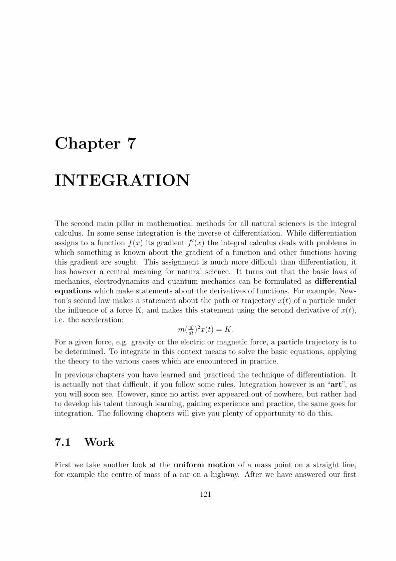
Chapter 7

INTEGRATION

The second main pillar in mathematical methods for all natural sciences is the integralcalculus. In some sense integration is the inverse of differentiation. While differentiationassigns to a function f(x) its gradient f ′(x) the integral calculus deals with problems inwhich something is known about the gradient of a function and other functions havingthis gradient are sought. This assignment is much more difficult than differentiation, ithas however a central meaning for natural science. It turns out that the basic laws ofmechanics, electrodynamics and quantum mechanics can be formulated as differentialequations which make statements about the derivatives of functions. For example, New-ton’s second law makes a statement about the path or trajectory x(t) of a particle underthe influence of a force K, and makes this statement using the second derivative of x(t),i.e. the acceleration:

m( ddt

)2x(t) = K.

For a given force, e.g. gravity or the electric or magnetic force, a particle trajectory is tobe determined. To integrate in this context means to solve the basic equations, applyingthe theory to the various cases which are encountered in practice.

In previous chapters you have learned and practiced the technique of differentiation. Itis actually not that difficult, if you follow some rules. Integration however is an “art”, asyou will soon see. However, since no artist ever appeared out of nowhere, but rather hadto develop his talent through learning, gaining experience and practice, the same goes forintegration. The following chapters will give you plenty of opportunity to do this.

7.1 Work

First we take another look at the uniform motion of a mass point on a straight line,for example the centre of mass of a car on a highway. After we have answered our first

121

question for the velocity with help of the differential calculus, we look as physicists to onelevel deeper for the reason: Why does the car move on this straight plane highway sectionwith the observed uniform speed? Obviously, the reason for the uniform straight motionaccording to Newton is a force, namely the force K, with which the engine pushes thecar against inertia, wind and other frictional loss. Latest at the gas station the questionarises how much work A has the engine done over the travelled distance ∆x. The workdone is proportional to the needed force was, and proportional to the travelled distance∆x. In fact it is exactly equal to the product of both quantities: A = K∆x, geometricallyequal to the rectangular area K times ∆x, if we draw in a Cartesian (i.e. right angled)coordinate system with the travelled distance x in the direction of the 1-axis and theoperating force K in direction of the 2-axis.

Figure 7.1: Constant force K as a function of the travelled distance from a tob = a+ ∆x. The yellow rectangular area is proportional to the work A = K∆x.

Following this idealized case of a constant operating force we turn our attention to a morerealistic case, where the force over the distance is increased linearly from an initialvalue K0 by giving more gas: K(x) = sx+K0 :

From the figure we immediately see how we can help ourselves, if the question arises (whilefilling up the gas tank) how much work was done over the entire distance. We take themean value ξ = (a+ b)/2 between the starting point a and the end point b, read out thecorresponding function value of the force K(ξ) = K((a + b)/2), and multiply this withthe travelled distance ∆x = b− a :

A = K(ξ)∆x = K(a+b2

)(b− a).

122

Figure 7.2: Force rising linearly with distance from the initial value K0 toK(x) = sx+K0 between the points a and b

In this way we reduce the physical question for the work to the geometrical question forthe “area under the force line over the interval ∆x”, more precisely for the contentof the area which is bordered on the top by a known function, to the left by the straightline x = a, to the right by the line x = b, and on the bottom by the 1-axis K(x) = 0.The advanced question for the work done by a force varying according to an arbitraryfunction is herewith traced back to the mathematical problem of the determination ofarea of a rectangle, in which one side (in this case the upper one) is replaced by a curve.In the following we would like to explore this more general mathematical question and togive an answer which will fulfill all wishes of physicists concerning work, and many otherwishes beyond.

7.2 Area under a Function over an Interval

We calculate the area F (f(x); a, b) “under” any bounded continuous, however for themoment positive function f(x) > 0 “over” the finite distance “between” the starting pointa and the final point b, also often called Fa(b)following the recipe indicated above forthe straight line: We divide the desired area in many narrow vertical strips, whose uppersides are nearly straight lines, calculate the areas of the strips as indicated above, sum upthe single parts and finally let the number of strips grow without limit in the hope thatthis way we will find the wanted area as the limiting value.

We want to document this limiting procedure just this once and then let it run in a

123

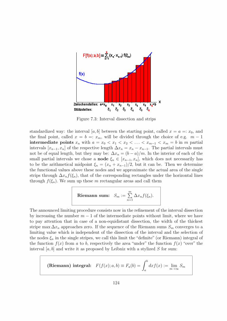
Figure 7.3: Interval dissection and strips

standardized way: the interval [a, b] between the starting point, called x = a =: x0, andthe final point, called x = b =: xm, will be divided through the choice of e.g. m − 1intermediate points xn with a = x0 < x1 < x2 < . . . < xm−1 < xm = b in m partialintervals [xn−1, xn] of the respective length ∆xn = xn − xn−1. The partial intervals mustnot be of equal length, but they may be: ∆xn = (b− a)/m. In the interior of each of thesmall partial intervals we chose a node ξn ∈ [xn−1, xn], which does not necessarily hasto be the arithmetical midpoint ξn = (xn + xn−1)/2, but it can be. Then we determinethe functional values above these nodes and we approximate the actual area of the singlestrips through ∆xnf(ξn), that of the corresponding rectangles under the horizontal linesthrough f(ξn). We sum up these m rectangular areas and call them

Riemann sum: Sm :=m∑n=1

∆xnf(ξn).

The announced limiting procedure consists now in the refinement of the interval dissectionby increasing the number m− 1 of the intermediate points without limit, where we haveto pay attention that in case of a non-equidistant dissection, the width of the thickeststripe max ∆xn approaches zero. If the sequence of the Riemann sums Sm converges to alimiting value which is independent of the dissection of the interval and the selection ofthe nodes ξn in the single stripes, we call this limit the “definite” (or Riemann) integral ofthe function f(x) from a to b, respectively the area “under” the function f(x) “over” theinterval [a, b] and write it as proposed by Leibniz with a stylized S for sum:

(Riemann) integral: F (f(x); a, b) ≡ Fa(b) =

∫ b

a

dxf(x) := limm→∞

Sm

124

The integrand f(x) may also be placed between the integral sign and the differential.

Mathematicians guarantee that the considered limit exists, if the integrand function f(x)is continuous and bounded, and the interval is finite and closed:

A bounded continuous function is (Riemann) integrable over a closedinterval.

In contrast to this, differentiability did not at all follow from continuity.

Insert: Calculation of an Integral According to the Definition: Afterthis complicated definition of the limiting procedure, clearly an example is needed:We choose the function f(x) = x2 and the interval [0, b]:

For the sake of simplicity, we divide the interval of length b through m−1 equidistantintermediate points xn = nb/m in m intervals of the uniform length ∆xn = b/m.As nodes in the intervals we choose the arithmetic means ξn = (xn + xn−1)/2 =(2n− 1)b/2m. With this we form the Riemann sums:

Sm :=m∑n=1

∆xnf(ξn) =m∑n=1

(bm

)((2n− 1)b

2m

)2=(bm

)3 (14

) m∑n=1

(2n− 1)2

The final sum causes a little trouble:

m∑n=1

(2n− 1)2 = 4

m∑n=1

n2 − 4

m∑n=1

n+

m∑n=1

n0

= 4m(m+ 1)(2m+ 1)/6− 4m(m+ 1)/2 +m

= m(4m2 − 1)/3.

Here we have used the sum of the first m numbersm∑n=1

n = m(m + 1)/2 and the

sum of the first m squaresm∑n=1

n2 = m(m + 1)(2m + 1)/6 from Chapter 2.1 and

m∑n=1

n0 = m. Thus we obtain for the sequence of the Riemann sums:

Sm := (b/m)3(1/4)m(4m2 − 1)/3 =b3

3

(1− 1

4m2

)and in the limit m→∞ : ∫ b

0dxx2 = lim

m→∞Sm =

b3

3.

125

The still-needed examination of whether the result is independent of the choice ofthe interval dissection and the choice of nodes we omitted.

This simple example shows us that on one hand the definition leads in fact to theexpected result, but on the other hand also how much effort is needed to calculatesuch a simple example according to the definition.

Therefore we will have to search for other methods to calculate integrals, and this

will be done in what follows.

7.3 Properties of the Riemann Integral

Before we go on to calculate further integrals, we want to get to know the most importantproperties of the derived integral concepts, and put them together. Also we want to freeourselves from some of the preconditions which until now we have accepted out of sheeridleness:

But first let us emphasize that the denotation of the integration variable x is ofcourse completely arbitrary: we also could have named it y:

∫ badxf(x) =

∫ badyf(y).

7.3.1 Linearity

From our knowledge of the characteristics of sums and the limits of sequences we can see,that the integral is linear, i.e. that the integral over a linear combination of functions isequal to the corresponding linear combination of the integrals of the single functions: forexample with two functions f(x) and g(x) and real constants c respectively d :

Linearity:

∫ b

a

dx(cf(x) + dg(x)) = c

∫ b

a

dxf(x) + d

∫ b

a

dxg(x).

The special case c = d = 1 is known as additivity of the integral:∫ b

a

dx(f(x) + g(x)) =

∫ b

a

dxf(x) +

∫ b

a

dxg(x).

An other special case is called homogeneity; when d = 0, it follows:∫ b

a

dxcf(x) = c

∫ b

a

dxf(x).

In particular for c = −1 that means:∫ b

a

dx(−f(x)) = F (−f(x); a, b) = −F (f(x); a, b) = −∫ b

a

dxf(x).

126

If f(x) ≥ 0, as assumed, is a positive function and F (f(x); a, b) =∫ badxf(x) the area

“under”the function, we see from the above relation that the integral over the negative, i.e.through the x-axis reflected function −f(x) ≤ 0, yields exactly −F (f(x); a, b), meaninga negative area. The area “above” the function −f(x) (running in the fourth quadrant)receives in the integral automatically a negative sign. We can therefore give up ourbeginner assumption f(x) ≥ 0, if we interpret the integral as area with sign: positive:“under” a function and above the x-axis, and negative: “above” a negative function andbelow the x-axis.

Figure 7.4: Functions f(x) and -f(x) with the coloured integral areas: F and -F.

If the integrand changes sign within the integration interval, the interval has to be dividedinto two parts, which must be treated separately and afterwards the results subtractedfrom each other with the proper sign.

7.3.2 Interval Addition

Next, we consider two adjoining integration intervals: i.e. two integrals, in which theupper limit of the first one coincides with the lower limit of the second integral whilethe integrand stays the same: From the meaning of the integral as area, there followsimmediately the so-called:

interval addition:

∫ b

a

dxf(x) +

∫ c

b

dxf(x) =

∫ c

a

dxf(x)

Thus we can for instance see without any calculation that∫ 2π

0dx sinx = 0.

With this knowledge we can free ourselves from a further beginner precondition, namelythat the upper limit b ≥ a has to be larger than or equal to the lower one, if we define:

127

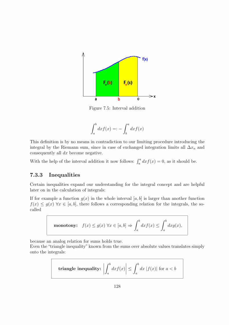
Figure 7.5: Interval addition

∫ b

a

dxf(x) =: −∫ a

b

dxf(x)

This definition is by no means in contradiction to our limiting procedure introducing theintegral by the Riemann sum, since in case of exchanged integration limits all ∆xn andconsequently all dx become negative.

With the help of the interval addition it now follows:∫ aadxf(x) = 0, as it should be.

7.3.3 Inequalities

Certain inequalities expand our understanding for the integral concept and are helpfullater on in the calculation of integrals:

If for example a function g(x) in the whole interval [a, b] is larger than another functionf(x) ≤ g(x) ∀x ∈ [a, b], there follows a corresponding relation for the integrals, the so-called

monotony: f(x) ≤ g(x) ∀x ∈ [a, b] ⇒∫ b

a

dxf(x) ≤∫ b

a

dxg(x),

because an analog relation for sums holds true.Even the “triangle inequality” known from the sums over absolute values translates simplyonto the integrals:

triangle inequality:

∣∣∣∣∫ b

a

dxf(x)

∣∣∣∣ ≤ ∫ b

a

dx |f(x)| for a < b

128

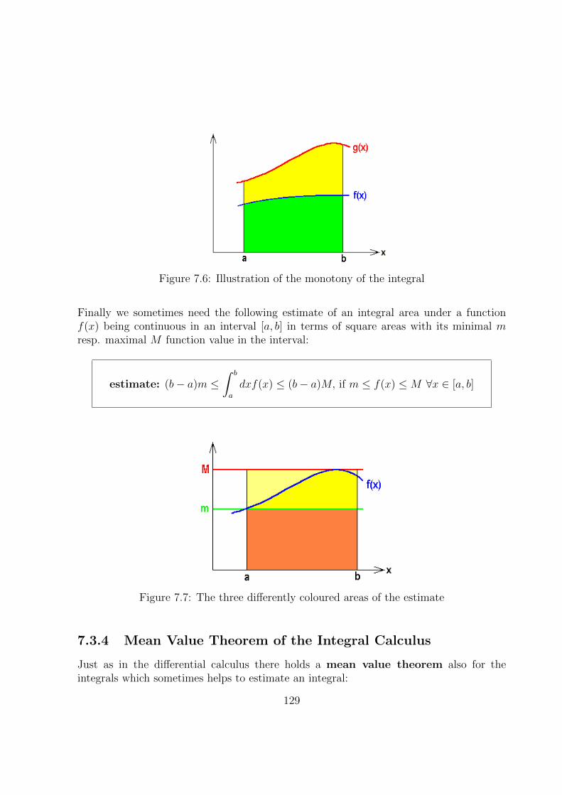
Figure 7.6: Illustration of the monotony of the integral

Finally we sometimes need the following estimate of an integral area under a functionf(x) being continuous in an interval [a, b] in terms of square areas with its minimal mresp. maximal M function value in the interval:

estimate: (b− a)m ≤∫ b

a

dxf(x) ≤ (b− a)M, if m ≤ f(x) ≤M ∀x ∈ [a, b]

Figure 7.7: The three differently coloured areas of the estimate

7.3.4 Mean Value Theorem of the Integral Calculus

Just as in the differential calculus there holds a mean value theorem also for theintegrals which sometimes helps to estimate an integral:

129

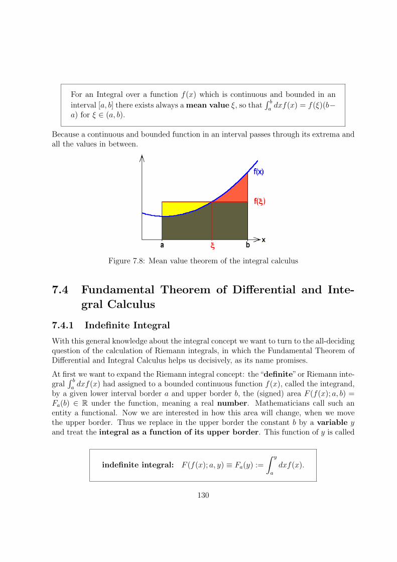
For an Integral over a function f(x) which is continuous and bounded in an

interval [a, b] there exists always a mean value ξ, so that∫ badxf(x) = f(ξ)(b−

a) for ξ ∈ (a, b).

Because a continuous and bounded function in an interval passes through its extrema andall the values in between.

Figure 7.8: Mean value theorem of the integral calculus

7.4 Fundamental Theorem of Differential and Inte-

gral Calculus

7.4.1 Indefinite Integral

With this general knowledge about the integral concept we want to turn to the all-decidingquestion of the calculation of Riemann integrals, in which the Fundamental Theorem ofDifferential and Integral Calculus helps us decisively, as its name promises.

At first we want to expand the Riemann integral concept: the“definite”or Riemann inte-gral

∫ badxf(x) had assigned to a bounded continuous function f(x), called the integrand,

by a given lower interval border a and upper border b, the (signed) area F (f(x); a, b) =Fa(b) ∈ R under the function, meaning a real number. Mathematicians call such anentity a functional. Now we are interested in how this area will change, when we movethe upper border. Thus we replace in the upper border the constant b by a variable yand treat the integral as a function of its upper border. This function of y is called

indefinite integral: F (f(x); a, y) ≡ Fa(y) :=

∫ y

a

dxf(x).

130

The procedure is fully analogous to the expansion step of the differential calculus fromthe gradient f ′(x0) of a function f(x) at a certain point x0 to the first derivative f ′(x) asa function of the variable x.

7.4.2 Differentiation with Respect to the Upper Border

In order to study the functional dependence of the indefinite integral from the variableupper border, we are at first interested in the gradient of the function Fa(y) :

(d

dy)Fa(y) := (

d

dy)

∫ y

a

dxf(x) = lim∆y→0

∫ y+∆y

adxf(x)−

∫ yadxf(x)

∆y=

if we insert the definition of the derivative. Because of the interval addition we get:

= lim∆y→0

∫ yadxf(x) +

∫ y+∆y

ydxf(x)−

∫ yadxf(x)

∆y= lim

∆y→0

∫ y+∆y

ydxf(x)

∆y=

According to the mean value theorem of the integral calculus there exists in the interval[y, y + ∆y] a mean value y + θ∆y with 0 ≤ θ ≤ 1, so that the following holds true:

= lim∆y→0

f(y + θ∆y)∆y

∆y= lim

∆y→0f(y + θ∆y) = f(y).

Altogether we get the

First part of the Fundamental Theorem: F ′a(y) := ( ddy

)

∫ y

a

dxf(x) =

f(y),i.e. the differential quotient of a indefinite integral with respect to its upperborder is the integrand taken at the upper border.

Exactly in this sense is differentiation the reversal of integration. For example ( ddy

)∫ y

0dt sin(ωt+

α) = sin(ωy + α) holds.

7.4.3 Integration of a Differential Quotient

After having learned to differentiate an integral, we are inquisitive about the reverseprocess, namely about the integral of a differential quotient: We start from the well-knowncontinuous differential quotient F ′(x) = f(x) which may be given to us as a continuousfunction f(x), i.e. really from a differential equation of the first order for F (x). We wantto integrate this differential quotient over the interval [a, b]:

131

∫ b

a

dxF ′(x) := limm→∞

m∑n=1

∆xnF′(ξn)

with the nodes ξn ∈ [xn−1, xn] within the interval of length ∆xn = xn − xn−1, if weinsert the definition of the integral. According to the Mean Value Theorem of DifferentialCalculus the gradient at the nodes ξn can be replaced by the gradient of the secant,meaning the replacement of the differential quotient by the difference quotient:

F ′(ξn) =F (xn)− F (xn−1)

xn − xn−1

.

Written in detail this yields:

limm→∞

((F (x1)−F(x0))+(F (x2)−F (x1))+. . .+(F (xm−1)−F (xm−2))+(F(xm)−F (xm−1))

).

We easily see that all terms are cancelling in pairs except the second and the second lastone, which do not at all depend on m and thus will not be affected by the limiting process:

... = F(xm)− F(x0) = F (b)− F (a) =: F (x)∣∣ba.

We therefore get altogether as

Second Part of the FUNDAMENTAL THEOREM:∫ badxF ′(x) = F (b)− F (a) =: F (x)

∣∣ba,

i.e. the definite integral of the differential quotient of a continuous differentiablefunction over an interval is equal to the difference of the function values at theupper and lower border of the interval.

Also in this sense integration is the reversal of differentiation.

For instance we get again the result: F (x2; 0, b) =∫ b

0dxx2 = b3/3, which we were hard put

to derive from the definition of the integral, but now effortlessly from the differentiation( ddx

)x3 = 3x2.

This second part of the Fundamental Theorem is the crucial step to the solution of ourintegration problem: Because we are now able to calculate all definite integrals of all thefunctions which we find in the second column of our Differentiation Table in Chapter5. We simply have to read the TABLE backward from right to left and complete theheading in the following accordingly:

132

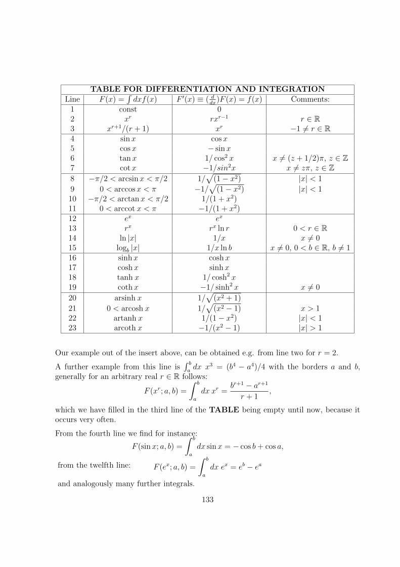
TABLE FOR DIFFERENTIATION AND INTEGRATION

Line F (x) =∫dxf(x) F ′(x) ≡ ( d

dx)F (x) = f(x) Comments:

1 const 02 xr rxr−1 r ∈ R3 xr+1/(r + 1) xr −1 6= r ∈ R4 sinx cosx5 cosx − sinx6 tanx 1/ cos2 x x 6= (z + 1/2)π, z ∈ Z7 cotx −1/sin2x x 6= zπ, z ∈ Z8 −π/2 < arcsinx < π/2 1/

√(1− x2) |x| < 1

9 0 < arccosx < π −1/√

(1− x2) |x| < 110 −π/2 < arctanx < π/2 1/(1 + x2)11 0 < arccot x < π −1/(1 + x2)12 ex ex

13 rx rx ln r 0 < r ∈ R14 ln |x| 1/x x 6= 015 logb |x| 1/x ln b x 6= 0, 0 < b ∈ R, b 6= 116 sinhx coshx17 coshx sinhx18 tanh x 1/ cosh2 x19 cothx −1/ sinh2 x x 6= 0

20 arsinh x 1/√

(x2 + 1)

21 0 < arcosh x 1/√

(x2 − 1) x > 122 artanh x 1/(1− x2) |x| < 123 arcoth x −1/(x2 − 1) |x| > 1

Our example out of the insert above, can be obtained e.g. from line two for r = 2.

A further example from this line is∫ badx x3 = (b4 − a4)/4 with the borders a and b,

generally for an arbitrary real r ∈ R follows:

F (xr; a, b) =

∫ b

a

dx xr =br+1 − ar+1

r + 1,

which we have filled in the third line of the TABLE being empty until now, because itoccurs very often.

From the fourth line we find for instance:

F (sinx; a, b) =

∫ b

a

dx sinx = − cos b+ cos a,

from the twelfth line: F (ex; a, b) =

∫ b

a

dx ex = eb − ea

and analogously many further integrals.

133

Exercise 7.1 Calculate the following examples of integrals:

a)

∫ 3

1

1

xdx, b)

∫ 1

−1

dx

1 + x2, c)

∫ b

0

dx√1 + x2

, d)

∫ 1/√

2

−1/√

2

dx√1− x2

,

e)

∫ a

−adx coshx , f)

∫ π/4

0

dx

cos2 x, g)

∫ 2

1

dx

x1+a, h)

∫ a

−adx x2n+1 for n ∈ Z

7.4.4 Primitive Function

Although we are able to calculate a considerable number of definite integrals over a largenumber of intervals, the question for the indefinite integral of a differential quotientF ′(x) = f(x) remains. We once again replace the constant upper border b of the definiteintegral through a variable y and as above we get∫ y

a

dxf(x) =

∫ y

a

dxF ′(x) = F (y)− F (a).

This we rewrite in the following way:

F (y) =

∫ y

a

dxf(x) + F (a) =:

∫ y

a

dxf(x) + c,

because with respect to the variable y F (a) is indeed a constant, although it depends onthe starting point of the interval a. Since we want to have the usual letter x as symbolfor the independent variable in the function F (y), an extraordinary sloppy way of writinghas sneaked into the above equation world-wide: symbolically it is written as:

F (x) =

∫dxf(x) + c and F (x) is called the primitive function of f(x).

The x on the left side serves only as a hint, that it is a function of an independent variable,and has obviously nothing to do with the really arbitrarily denotable integration variablex on the right hand side, which obviously does not occur anymore after the integration onthe right side. Once we have cleared up this sloppy mess, it is quite a comfortable matterand acknowledged world-wide.

Written in such a sloppy way, the primitive function is actually a whole family of functionswith the family parameter c. The primitive function F (x) of f(x) is exactly the familyof functions which solves our original differential equation F ′(x) = f(x) and that is thereason why it is so important for physicists. Out of this family with pre-given gradientf(x), the physicist has to only pick out the solution by choosing the constant c so thatthe function fulfils the correct boundary condition c = F (a), and the problem is solved.

134

For example, the primitive function F (x) of f(x) = 3x is searched for, which fulfils theboundary condition F (1) = 2. Out of the function family F (x) = 3x2/2 + c we have tochoose the function which fulfills F (1) = 3/2 + c = 2, meaning c = 1/2: consequentlyF (x) = (3x2 + 1)/2 is the desired solution.

Exercise 7.2 Determine the primitive functions of the following functions:

a) f(x) = x3 , b) f(x) =1√

x2 − 1, c) f(x) = sinh x and d) f(x) = 2x

Exercise 7.3 Determine the primitive functions of the following functions with the givenboundary conditions:

a) f(x) = sinx with F (π) = 1, b) f(x) =1√x

with F (4) = 1 and

c) f(x) =1

cosh2 xwith F (a) = 1

2

7.5 The Art of Integration

In this chapter we want to put together what we need for the integration of the functionsfrom our basic set and those assembled from it.

Initially after the discoveries of the Fundamental Theorem, we have the recipe: read thedifferentiation table backwards.

7.5.1 Differentiation Table Backwards

For example from line 14 we get:∫ e

1dx/x = lnx

∣∣e1

= ln e− ln 1 = 1− 0 = 1

or from line 4:∫ π/2

0dt cos t = sin t

∣∣π/20

= sin(π/2)− sin 0 = 1− 0 = 1

or from line 10:∫ badx/(x2 + 1) = arctanx

∣∣ba

or from line 8 indefinitely:∫dx/√

(1− x2) = arcsin x+ c.

In our first enthusiasm for the consequences of the Fundamental Theorem for integration,by reading the differentiation table backwards, we have slightly overrated our success.Because upon closer inspection, we see that there are only relatively few functions, that

135

occur in the second column of our TABLE. Even such simple functions out of our basicset as f(x) = x2 + 1 cannot be found. All the more f(x) =

√(1− x2) is nowhere to be

found, although we can easily integrate the reciprocal of this root. Also with the Gaussianbell-shaped f(x) = exp(−x2) we are pretty helpless with out TABLE.

Differently as in differentiation there is no procedure of integration which automaticallyafter a sufficient amount of work leads to the goal. This is the reason why integrationis an art while differentiation can be called atechnique.

Nevertheless, there are a lot of rules and tricks which follow from the characteristics ofthe integral and can make our lives considerably easier. Therefore we want to turn outattention now to those: the simplest one is the linear decomposition.

7.5.2 Linear Decomposition

We have seen in Chapter 7.3.1, that the integral is a linear operation:

∫ b

a

dx(cf(x) + dg(x)) = c

∫ b

a

dxf(x) + d

∫ b

a

dxg(x).

We will use this recipe in a large number of integrals, e.g. in determining the area of theyellow “leaf” in the following figure:

Figure 7.9a: Integral over the “leaf”

136

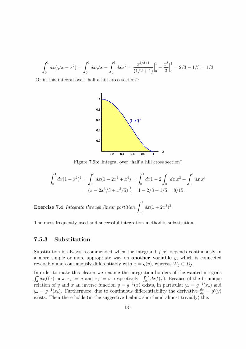
∫ 1

0

dx(√x− x2) =

∫ 1

0

dx√x−

∫ 1

0

dxx2 =x1/2+1

(1/2 + 1)

∣∣∣10− x3

3

∣∣∣10

= 2/3− 1/3 = 1/3

Or in this integral over “half a hill cross section”:

Figure 7.9b: Integral over “half a hill cross section”

∫ 1

0

dx(1− x2)2 =

∫ 1

0

dx(1− 2x2 + x4) =

∫ 1

0

dx1− 2

∫ 1

0

dx x2 +

∫ 1

0

dx x4

= (x− 2x3/3 + x5/5)∣∣10

= 1− 2/3 + 1/5 = 8/15.

Exercise 7.4 Integrate through linear partition

∫ 1

−1

dx(1 + 2x3)3.

The most frequently used and successful integration method is substitution.

7.5.3 Substitution

Substitution is always recommended when the integrand f(x) depends continuously ina more simple or more appropriate way on another variable y, which is connectedreversibly and continuously differentiably with x = g(y), whereas Wg ⊂ Df .

In order to make this clearer we rename the integration borders of the wanted integrals∫ badxf(x) now xa := a and xb := b, respectively:

∫ xbxadxf(x). Because of the bi-unique

relation of y and x an inverse function y = g−1(x) exists, in particular ya = g−1(xa) andyb = g−1(xb). Furthermore, due to continuous differentiability the derivative dx

dy= g′(y)

exists. Then there holds (in the suggestive Leibniz shorthand almost trivially) the:

137

substitution formula

∫ xb

xa

dxf(x) =

∫ yb

ya

dy(dx

dy)f(g(y)) =

∫ yb

ya

dyg′(y)f(g(y)).

Insert: Proof of the Substitution Formula: If the primitive function F (x)of the integrand f(x), i.e. the solution of the differential equation ( d

dx)F (x) = f(x)were known, then from the second part of the Fundamental Theorem for the left sideof the equation would follow∫ xb

xa

dxf(x) = F (xb)− F (xa).

If we assume that the solution of the differential equation ( ddy )F (g(y)) = f(g(y))g′(y)

is known, i.e. F (g(y)) is the primitive function of f(g(y))g′(y) as function of theother variable y, then for the right hand side of the equation follows from the Fun-damental Theorem:∫ yb

ya

dy g′(y)f(g(y)) = F (g(yb))− F (g(ya)) = F (xb)− F (xa)

with x = g(y) as stated above.

From experience, the explanation of the substitution procedure is more complicated thanthis method in practice. Here are some typical examples:∫ 5

1

dx√

(2x− 1) = ... with xa = 1 and xb = 5.

As new variable y := 2x − 1 is pretty obvious with ya = 2 · 1 − 1 = 1, yb = 2 · 5 − 1 = 9and dy

dx= 2, so dx

dy= 1/2. Thus it follows:

... =

∫ 9

1

dydx

dyy1/2 = (1/2)y3/2/(3/2)

∣∣91

= (9 · 3− 1)/3 = 26/3.

An important example for physics is:∫ π

0

dt cosωt = ... with ta = 0 and tb = π.

We chose the substitution y := ωt with ya = 0, yb = ωπ and dydt

= ω, so dtdy

= 1/ω. Thuswe get:

... =

∫ ωπ

0

dy( dtdy

) cos y = (1/ω) sin y∣∣ωπ0

= (1/ω) sinωπ.

A third example from physics:

138

∫ b

0

dt t exp(−αt2) = ... with ta = 0 and tb = b.

We substitute y := −αt2 with ya = 0, yb = −αb2 and dydt

= −2αt, so dtdy

= −1/2αt. Fromthis we get:

... =

∫ −αb20

dy( dtdy

)t exp y = (−1/2α) exp y∣∣−αb20

= (1− exp(−αb2))/2α.

Exercise 7.5 Substitution

a)

∫dx/(ax+ b), b)

∫ t

0

dx e−2x/a, c)

∫ 1

0

dx√

(1− x2),

d)

∫ r

0

dx√r2 − x2, e)

∫dt x(t), f)

∫ a

−adx cosh(x/A)

We obtain even classes of integrals in the following way by using the “substitutionformula backward”. What we mean by this is best explained through the followingexamples:

Supposing we have to calculate an integral of the following type, where we have sugges-tively chosen y for the arbitrary integration variable:∫ yb

ya

dy g′(y)/g(y) = ...

This is obviously the right side of our substitution formula, especially for the functionf(x) = 1/x and we can apply the substitution formula immediately with x = g(y) fromright to left, i.e. “backwards”, in order to find:

... =

∫ xb

xa

dx

x. This however, according to line 14 of our TABLE is equal to

... = ln |x|∣∣xbxa

and with x = g(y) it follows altogether:

∫ yb

ya

dy g′(y)/g(y) = ln |g(y)|∣∣ybya.

As examples we have:

139

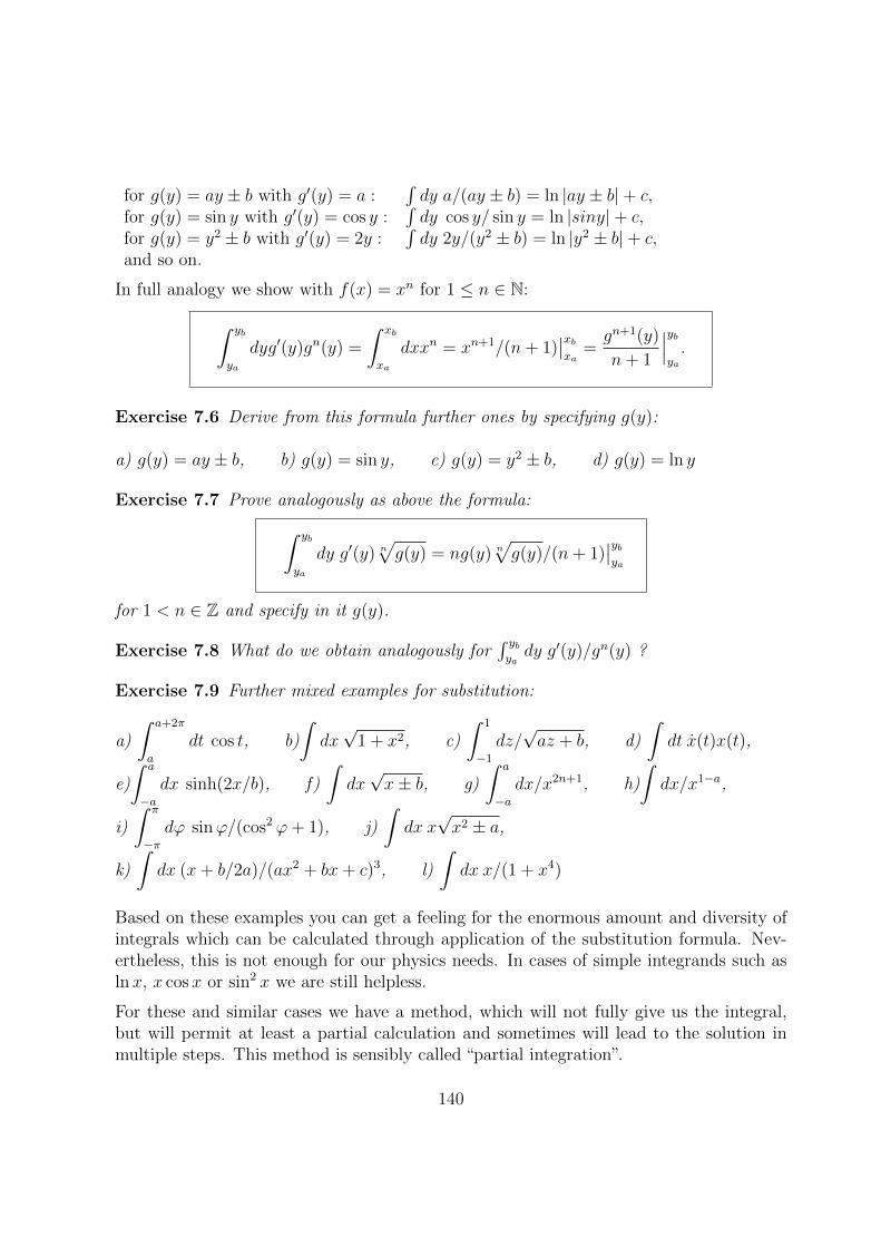
for g(y) = ay ± b with g′(y) = a :∫dy a/(ay ± b) = ln |ay ± b|+ c,

for g(y) = sin y with g′(y) = cos y :∫dy cos y/ sin y = ln |siny|+ c,

for g(y) = y2 ± b with g′(y) = 2y :∫dy 2y/(y2 ± b) = ln |y2 ± b|+ c,

and so on.

In full analogy we show with f(x) = xn for 1 ≤ n ∈ N:

∫ yb

ya

dyg′(y)gn(y) =

∫ xb

xa

dxxn = xn+1/(n+ 1)∣∣xbxa

=gn+1(y)

n+ 1

∣∣∣ybya.

Exercise 7.6 Derive from this formula further ones by specifying g(y):

a) g(y) = ay ± b, b) g(y) = sin y, c) g(y) = y2 ± b, d) g(y) = ln y

Exercise 7.7 Prove analogously as above the formula:∫ yb

ya

dy g′(y) n√g(y) = ng(y) n

√g(y)/(n+ 1)

∣∣ybya

for 1 < n ∈ Z and specify in it g(y).

Exercise 7.8 What do we obtain analogously for∫ ybyady g′(y)/gn(y) ?

Exercise 7.9 Further mixed examples for substitution:

a)

∫ a+2π

a

dt cos t, b)

∫dx√

1 + x2, c)

∫ 1

−1

dz/√az + b, d)

∫dt x(t)x(t),

e)

∫ a

−adx sinh(2x/b), f)

∫dx√x± b, g)

∫ a

−adx/x2n+1, h)

∫dx/x1−a,

i)

∫ π

−πdϕ sinϕ/(cos2 ϕ+ 1), j)

∫dx x√x2 ± a,

k)

∫dx (x+ b/2a)/(ax2 + bx+ c)3, l)

∫dx x/(1 + x4)

Based on these examples you can get a feeling for the enormous amount and diversity ofintegrals which can be calculated through application of the substitution formula. Nev-ertheless, this is not enough for our physics needs. In cases of simple integrands such aslnx, x cosx or sin2 x we are still helpless.

For these and similar cases we have a method, which will not fully give us the integral,but will permit at least a partial calculation and sometimes will lead to the solution inmultiple steps. This method is sensibly called “partial integration”.

140

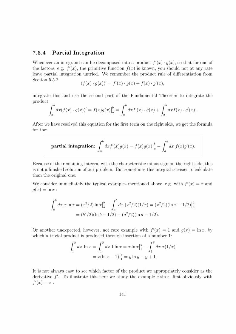
7.5.4 Partial Integration

Whenever an integrand can be decomposed into a product f ′(x) · g(x), so that for one ofthe factors, e.g. f ′(x), the primitive function f(x) is known, you should not at any rateleave partial integration untried. We remember the product rule of differentiation fromSection 5.5.2:

(f(x) · g(x))′ = f ′(x) · g(x) + f(x) · g′(x),

integrate this and use the second part of the Fundamental Theorem to integrate theproduct:∫ b

a

dx(f(x) · g(x))′ = f(x)g(x)∣∣ba

=

∫ b

a

dxf ′(x) · g(x) +

∫ b

a

dxf(x) · g′(x).

After we have resolved this equation for the first term on the right side, we get the formulafor the:

partial integration:

∫ b

a

dxf ′(x)g(x) = f(x)g(x)∣∣ba−∫ b

a

dx f(x)g′(x).

Because of the remaining integral with the characteristic minus sign on the right side, thisis not a finished solution of our problem. But sometimes this integral is easier to calculatethan the original one.

We consider immediately the typical examples mentioned above, e.g. with f ′(x) = x andg(x) = lnx :∫ b

a

dx x lnx = (x2/2) lnx∣∣ba−∫ b

a

dx (x2/2)(1/x) = (x2/2)(lnx− 1/2)∣∣ba

= (b2/2)(ln b− 1/2)− (a2/2)(ln a− 1/2).

Or another unexpected, however, not rare example with f ′(x) = 1 and g(x) = lnx, bywhich a trivial product is produced through insertion of a number 1:∫ y

1

dx lnx =

∫ y

1

dx 1 lnx = x lnx∣∣y1−∫ y

1

dx x(1/x)

= x(lnx− 1)∣∣y1

= y ln y − y + 1.

It is not always easy to see which factor of the product we appropriately consider as thederivative f ′. To illustrate this here we study the example x sinx, first obviously withf ′(x) = x :

141

∫ y

0

dx x sinx = (x2/2) sinx∣∣y0−∫ y

0

dx(x2/2) cosx.

We see immediately that this choice will not get us further. Instead, it makes the remainingintegrand even more complicated. The other possibility f ′(x) = sinx leads to success:

∫ y

0

dx x sinx = −x cosx∣∣y0−∫ y

0

dx 1(− cosx) = −y cos y + sinx∣∣y0

= −y cos y + sin y.

As a further example we consider the integrand x2 cosx and choose based on our experiencefrom just above f ′(x) = cos x :∫ y

0

dx x2 cosx = x2 sinx∣∣y0−∫ y

0

dx 2x sinx = y2 sin y − 2

∫ y

0

dx x sinx.

Although this is not the solution to our problem, it is a step in the right direction, sincewe have just calculated the remaining integral in our last example. With this result itfollows: ∫ y

0

dx x2 cosx = y2 sin y + 2y cos y − 2 sin y.

Altogether, a double partial integration has lead us here to the solution.

A further interesting example is (for a change an indefinite integral):∫dx cosx sinx = sinx sinx−

∫dx sinx cosx+ c.

The remaining integral is equal to the original one, hence we get with a new c :∫dx cosx sinx =

sin2 x

2+ c.

The next example with f ′(x) = g(x) = sinx is also remarkable:∫dx sin2 x = − cosx sinx−

∫dx(− cosx) cosx = − cosx sinx+

∫dx cos2 x = ...

After inserting the relation cos2 x+ sin2 x = 1, we get:

... = − cosx sinx+

∫dx(1− sin2x) = x− cosx sinx−

∫dx sin2 x = (x− cosx sinx)/2.

142

An entire series of examples of this kind follows with f ′(x) = e−x, for which a specialnotation was created because of their importance in physics:

E1(y) =

∫ y

0

dx xe−x = −xe−x∣∣y0

+

∫ y

0

dx 1e−x = −ye−x + 0− e−x∣∣y0

= −ye−y + e−y − 1

E2(y) =

∫ y

0

dx x2e−x = −x2e−x∣∣y0

+

∫ y

0

dx 2xe−x = −y2e−y + 2E1(y)

...

En(y) =

∫ y

0

dx xne−x = −yne−y + nEn−1(y).

Exercise 7.10 Integrate the following integrals by partial integration:

a)

∫ y

0

dx sinx e−x, b)

∫ y

0

dx cosx e−x, c)

∫dx arcsinx, d)

∫dx x√

1 + x,

e)

∫dx x3 exp(x2), f)

∫dx x2 lnx, g)

∫dx ln(x2 + 1)

and prove the following useful recursion formulae for n ∈ N:

h)

∫dx f ′(x)xn = f(x)xn − n

∫dx f(x)xn−1,

i)

∫dx g(x)/xn = −g(x)/(n− 1)xn−1 +

∫dx g′(x)/(n− 1)xn−1 for n 6= 1,

j)

∫dx sinn x = − 1

ncosx sinn−1 x+

n− 1

n

∫dx sinn−2 x,

k)

∫dx (1± x2)n = x

(1± x2)n

2n+ 1+ 2n

∫dx

(1± x2)n−1

2n+ 1

Exercise 7.11 Show that for the motion of a mass point on a straight line the traveleddistance x(t) can be calculated from a pre-given acceleration function a(t) with startingvelocity v0 and position x0 by partial integration in the following form: x(t) =

∫ t0dy(t −

y)a(y) + v0t+ x0.

7.5.5 Further Integration Tricks

Apart from substitution and partial integration with their broad field of application thereare a whole range of further integration tricks, mostly for a limited classes of integrals.As representative for these, we want to take a closer look at the Hermite ansatz, whichexpresses integrals of type

∫dxPm(x)/Γ(x) with a polynomial Pm(x) of the m-th degree

over a root Γ(x) :=√

(ax2 + bx+ c) of a quadratic expression, in terms of the correspond-ing integral with the polynomial 1, because these kinds of integrands are very common inphysics. Hermite made the following ansatz:

143

Hermite ansatz:∫dxPm(x)/Γ(x) = Qm−1(x)Γ(x) + am

∫dx/Γ(x) with Qm−1(x) :=

m−1∑n=0

anxn

with a polynomial of the (m − 1)-th degree Qm−1(x) and real numbers am. We get therequired (m+ 1) numbers an with n = 0, 1, 2, . . . ,m through coefficient comparison of thefollowing two polynomials of m-th degree:

Pm(x) = Q′m−1(x)Γ2(x) + (ax+ b/2)Qm−1(x) + am

The differentiation of the Hermite ansatz yields

Pm(x)/Γ(x) = Q′m−1(x)Γ(x) +Qm−1(x)Γ′(x) + am/Γ(x)

= Q′m−1(x)Γ(x) +Qm−1(x)(2ax+ b)/2Γ(x) + am/Γ(x)

and multiplication with Γ(x) gives the above determination equation for the (m + 1)coefficients an.

Exercise 7.12 Show that the coefficient comparison

a) for P3(x) = 3x3 + 5x2 + 3x and Γ(x) =√

(x2 + 2x+ 2) leads to a3 = a2 = 1, a1 = 0and a0 = −1, so that Q2(x) = x2 − 1 follows and

b) for P2(x) = x2 and Γ(x) =√

1− x2 leads to a2 = 1/2, a1 = −1/2 and a0 = 0with Q1(x) = −x/2 as solution.

The remaining integrals of type∫dx/Γ(x) we solve by a trick, known to many of you

from school, namely the quadratic completion, i.e. addition and subtraction of thesame term (here bold printed): if e.g. a > 0

∫dx/Γ(x) =

∫dx/√

(ax2 + bx+ c)

= (1/√a)

∫dx/√x2 + bx/a+ (b/2a)2 + c/a− (b/2a)2

= (1/√a)

∫dx/√

(x+ b/2a)2 + ∆/4a2

144

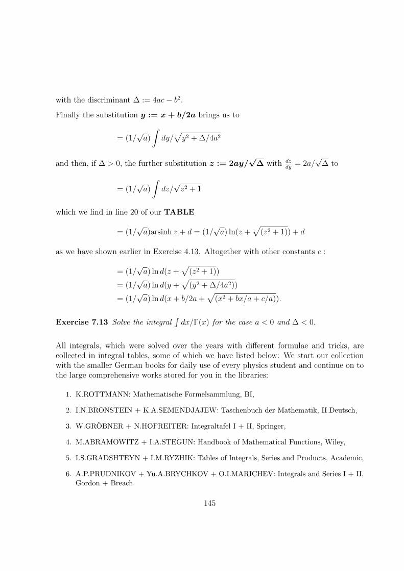
with the discriminant ∆ := 4ac− b2.

Finally the substitution y := x+ b/2a brings us to

= (1/√a)

∫dy/√y2 + ∆/4a2

and then, if ∆ > 0, the further substitution z := 2ay/√

∆ with dzdy

= 2a/√

∆ to

= (1/√a)

∫dz/√z2 + 1

which we find in line 20 of our TABLE

= (1/√a)arsinh z + d = (1/

√a) ln(z +

√(z2 + 1)) + d

as we have shown earlier in Exercise 4.13. Altogether with other constants c :

= (1/√a) ln d(z +

√(z2 + 1))

= (1/√a) ln d(y +

√(y2 + ∆/4a2))

= (1/√a) ln d(x+ b/2a+

√(x2 + bx/a+ c/a)).

Exercise 7.13 Solve the integral∫dx/Γ(x) for the case a < 0 and ∆ < 0.

All integrals, which were solved over the years with different formulae and tricks, arecollected in integral tables, some of which we have listed below: We start our collectionwith the smaller German books for daily use of every physics student and continue on tothe large comprehensive works stored for you in the libraries:

1. K.ROTTMANN: Mathematische Formelsammlung, BI,

2. I.N.BRONSTEIN + K.A.SEMENDJAJEW: Taschenbuch der Mathematik, H.Deutsch,

3. W.GROBNER + N.HOFREITER: Integraltafel I + II, Springer,

4. M.ABRAMOWITZ + I.A.STEGUN: Handbook of Mathematical Functions, Wiley,

5. I.S.GRADSHTEYN + I.M.RYZHIK: Tables of Integrals, Series and Products, Academic,

6. A.P.PRUDNIKOV + Yu.A.BRYCHKOV + O.I.MARICHEV: Integrals and Series I + II,Gordon + Breach.

145

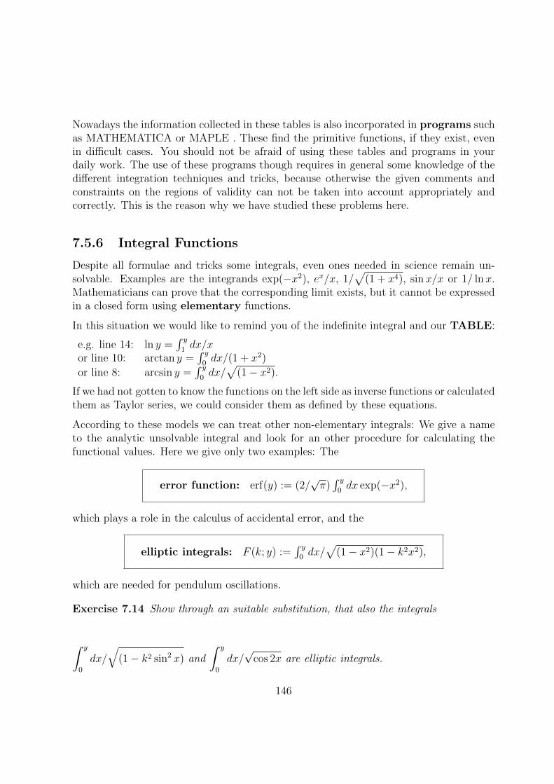
Nowadays the information collected in these tables is also incorporated in programs suchas MATHEMATICA or MAPLE . These find the primitive functions, if they exist, evenin difficult cases. You should not be afraid of using these tables and programs in yourdaily work. The use of these programs though requires in general some knowledge of thedifferent integration techniques and tricks, because otherwise the given comments andconstraints on the regions of validity can not be taken into account appropriately andcorrectly. This is the reason why we have studied these problems here.

7.5.6 Integral Functions

Despite all formulae and tricks some integrals, even ones needed in science remain un-solvable. Examples are the integrands exp(−x2), ex/x, 1/

√(1 + x4), sinx/x or 1/ lnx.

Mathematicians can prove that the corresponding limit exists, but it cannot be expressedin a closed form using elementary functions.

In this situation we would like to remind you of the indefinite integral and our TABLE:

e.g. line 14: ln y =∫ y

1dx/x

or line 10: arctan y =∫ y

0dx/(1 + x2)

or line 8: arcsin y =∫ y

0dx/√

(1− x2).

If we had not gotten to know the functions on the left side as inverse functions or calculatedthem as Taylor series, we could consider them as defined by these equations.

According to these models we can treat other non-elementary integrals: We give a nameto the analytic unsolvable integral and look for an other procedure for calculating thefunctional values. Here we give only two examples: The

error function: erf(y) := (2/√π)∫ y

0dx exp(−x2),

which plays a role in the calculus of accidental error, and the

elliptic integrals: F (k; y) :=∫ y

0dx/√

(1− x2)(1− k2x2),

which are needed for pendulum oscillations.

Exercise 7.14 Show through an suitable substitution, that also the integrals

∫ y

0

dx/√

(1− k2 sin2 x) and

∫ y

0

dx/√

cos 2x are elliptic integrals.

146

Figure 7.11: Error function

Obviously the beautiful name alone does not help. A method must be found which allowsthe calculation of the functional values. When all other means fail, we have no choice butthe numerical integration.

7.5.7 Numerical Integration

The oldest and most primitive way to determine a definite integral, i.e. to calculate thearea “under” a function “over” an interval, is of course to draw the integrand onto graphpaper and then count the squares.

With today’s electronic calculators we can do this more elegantly and much faster, byconsidering the defining limit and summing up the areas of the strips after the dissectionof the interval. In doing so, the fewer strips and steps of iteration are needed, the closerwe fit the upper edge of the strip to the actual function to be integrated.

The simplest choice are the horizontal straight lines as we have done in the definition, sothat the strips become rectangles, whose areas are easy to calculate. Instead of the nodesξn in the interior of the partial intervals just as with the Riemann sum, we can also takethe minima and maxima of the function in the partial intervals. Then we obtain an underand over sum, which enclose the integral in the limit.

The next elegant method is the chord-trapezium rule, by which the function in eachpartial interval is approximated through the secant, and the real areas of the stripesthrough the areas of trapezia. For each partial interval we take instead of ∆xnf(ξn) :

(∆xn)(f(xn−1) + f(xn))/2.

147

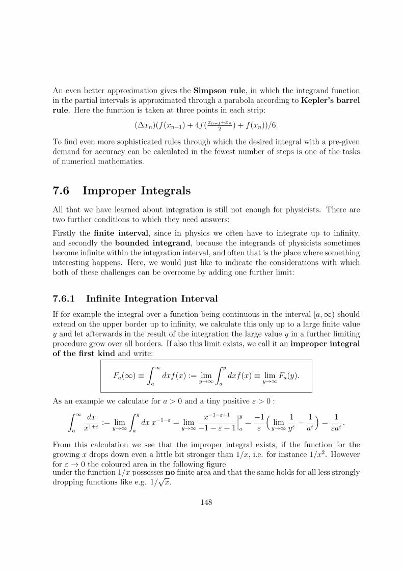
An even better approximation gives the Simpson rule, in which the integrand functionin the partial intervals is approximated through a parabola according to Kepler’s barrelrule. Here the function is taken at three points in each strip:

(∆xn)(f(xn−1) + 4f(xn−1+xn2

) + f(xn))/6.

To find even more sophisticated rules through which the desired integral with a pre-givendemand for accuracy can be calculated in the fewest number of steps is one of the tasksof numerical mathematics.

7.6 Improper Integrals

All that we have learned about integration is still not enough for physicists. There aretwo further conditions to which they need answers:

Firstly the finite interval, since in physics we often have to integrate up to infinity,and secondly the bounded integrand, because the integrands of physicists sometimesbecome infinite within the integration interval, and often that is the place where somethinginteresting happens. Here, we would just like to indicate the considerations with whichboth of these challenges can be overcome by adding one further limit:

7.6.1 Infinite Integration Interval

If for example the integral over a function being continuous in the interval [a,∞) shouldextend on the upper border up to infinity, we calculate this only up to a large finite valuey and let afterwards in the result of the integration the large value y in a further limitingprocedure grow over all borders. If also this limit exists, we call it an improper integralof the first kind and write:

Fa(∞) ≡∫ ∞a

dxf(x) := limy→∞

∫ y

a

dxf(x) ≡ limy→∞

Fa(y).

As an example we calculate for a > 0 and a tiny positive ε > 0 :∫ ∞a

dx

x1+ε:= lim

y→∞

∫ y

a

dx x−1−ε = limy→∞

x−1−ε+1

−1− ε+ 1

∣∣∣ya

=−1

ε

(limy→∞

1

yε− 1

aε

)=

1

εaε.

From this calculation we see that the improper integral exists, if the function for thegrowing x drops down even a little bit stronger than 1/x, i.e. for instance 1/x2. Howeverfor ε→ 0 the coloured area in the following figureunder the function 1/x possesses no finite area and that the same holds for all less stronglydropping functions like e.g. 1/

√x.

148

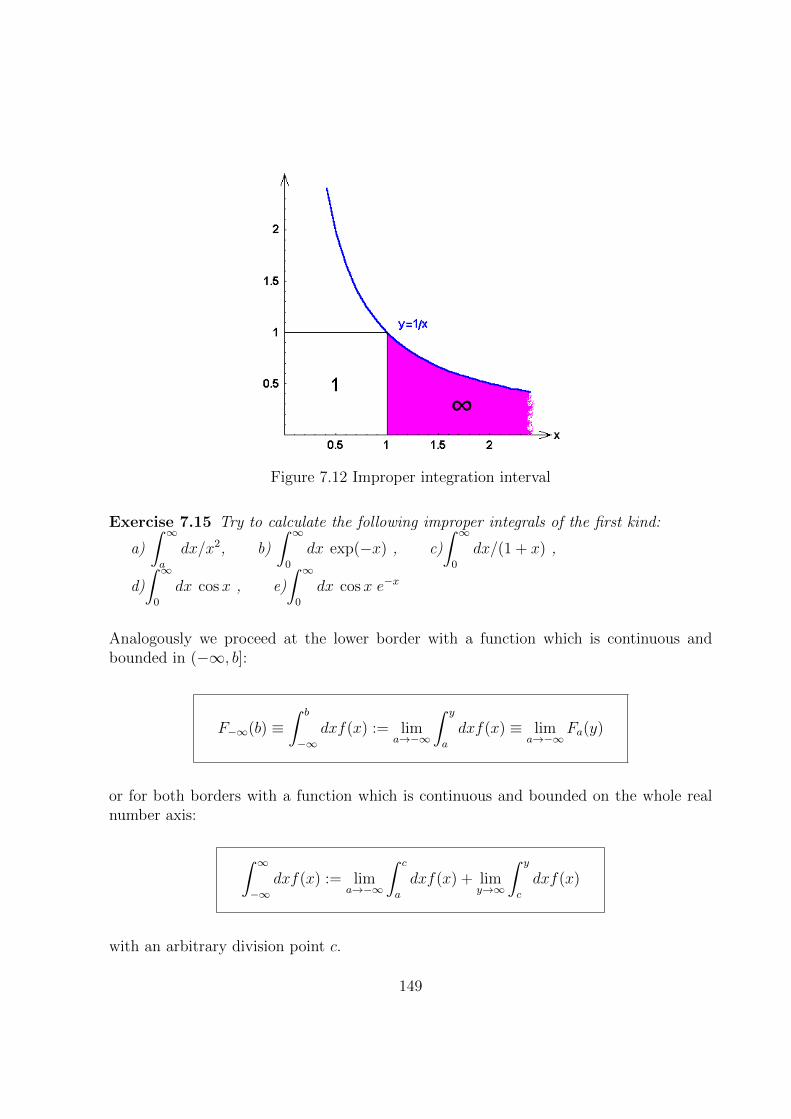
Figure 7.12 Improper integration interval

Exercise 7.15 Try to calculate the following improper integrals of the first kind:

a)

∫ ∞a

dx/x2, b)

∫ ∞0

dx exp(−x) , c)

∫ ∞0

dx/(1 + x) ,

d)

∫ ∞0

dx cosx , e)

∫ ∞0

dx cosx e−x

Analogously we proceed at the lower border with a function which is continuous andbounded in (−∞, b]:

F−∞(b) ≡∫ b

−∞dxf(x) := lim

a→−∞

∫ y

a

dxf(x) ≡ lima→−∞

Fa(y)

or for both borders with a function which is continuous and bounded on the whole realnumber axis:

∫ ∞−∞

dxf(x) := lima→−∞

∫ c

a

dxf(x) + limy→∞

∫ y

c

dxf(x)

with an arbitrary division point c.

149

Exercise 7.16 Calculate:

∫ −2/π

−∞dx sin(1/x)/x2 and

∫ 0

−∞dx x/(1 + x4).

Insert: Cauchy Principal Value: It is possible that both the limits existonly if the huge finite borders grow in the same manner. In this case the resultis called

Cauchy principal value: P

∫ ∞−∞

dxf(x) := limc→∞

∫ c

−cdxf(x).

In order to illustrate this we calculate the following example for n ∈ N:

∫ ∞−∞

dx x2n−1 := lima→−∞

∫ c

adx x2n−1 + lim

y→∞

∫ y

cdx x2n−1

= lima→−∞

(−a2n/2n) + limy→∞

y2n/2n.

Apparently both the limits do not exist. If we, however, form the principal value,there follows:

P

∫ ∞−∞

dx x2n−1 := limc→∞

∫ c

−cdx x2n−1 = lim

c→∞0 = 0,

since once again the integral of an odd function over an interval symmetric to the

origin vanishes.


∫ ∞−∞

dx/(1 + x2) and

∫ ∞−∞

dx x/(1 + x4).

7.6.2 Unbounded Integrand

We now take a quick look at the second case, namely when the integrand is unboundedat a point x0 of the finite integration interval [a, b], e.g. on the lower border: x0 = a. Wecalculate in this case the integral starting from the value x0 + η, which lies only a tinydistance η > 0 above the critical point x0 and let only in the result of the integration thistiny distance approach zero. If this limit exists, we call it an improper integral of thesecond kind and write:

150

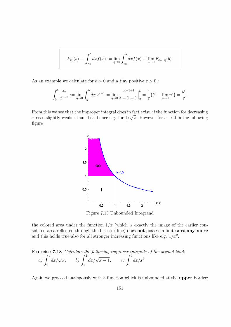
Fx0(b) ≡∫ b

x0

dxf(x) := limη→0

∫ b

x0

dxf(x) ≡ limη→0

Fx0+η(b).

As an example we calculate for b > 0 and a tiny positive ε > 0 :∫ b

0

dx

x1−ε := limη→0

∫ b

η

dx xε−1 = limη→0

xε−1+1

ε− 1 + 1

∣∣∣bη

=1

ε

(bε − lim

η→0ηε)

=bε

ε.

From this we see that the improper integral does in fact exist, if the function for decreasingx rises slightly weaker than 1/x, hence e.g. for 1/

√x. However for ε→ 0 in the following

figure

Figure 7.13 Unbounded Integrand

the colored area under the function 1/x (which is exactly the image of the earlier con-sidered area reflected through the bisector line) does not possess a finite area any moreand this holds true also for all stronger increasing functions like e.g. 1/x2.

Exercise 7.18 Calculate the following improper integrals of the second kind:

a)

∫ b

0

dx/√x, b)

∫ 2

1

dx/√x− 1, c)

∫ b

0

dx/x3

Again we proceed analogously with a function which is unbounded at the upper border:

151

Fa(x0) ≡∫ x0

a

dxf(x) := limε→0

∫ x0−ε

a

dxf(x) ≡ limε→0

Fa(x0 − ε)

or in case the function is unbounded within the integration interval at a point x0:

∫ b

a

dxf(x) := limε→0

∫ x0−ε

a

dxf(x) + limη→0

∫ b

x0+η

dxf(x).

Insert: Cauchy Principal Value: Here it is possible that both the limitsexist only, if the tiny distances ε and η off the critical point vanish in the samemanner. Also in this case the result is called

Cauchy principal value: P

∫ b

adxf(x) := lim

ε→0

( ∫ x0−ε

adxf(x) +

∫ b

x0+εdxf(x)

).

The following example may explain this for n ∈ N:

∫ b>0

a<0dx/x2n+1 := lim

ε→0

∫ −εa

dx/x2n+1 + limη→0

∫ b

ηdx/x2n+1

= limε→0

x−2n/(−2n)∣∣−εa

+ limη→0

x−2n/(−2n)∣∣bη

Also here both the limits do not exist. If we, however, form the principal value e.g.for a = −b, it follows:

P

∫ b

−bdx/x2n+1 := lim

η→0

∫ b

−bdx/x2n+1 = lim

η→00 = 0,

since once again the integral of an odd function over an interval symmetric to the

origin vanishes.


∫ 1

0

dx/√

1− x2 and

∫ π/2

0

dx tanx.

Exercise 7.20 Calculate: P

∫ 2

−1

dx/x and P

∫ π

0

dx tanx.

152

Exercise 7.21 Show that the improper integral of the second kind:∫ 1

0dx/√x through the

substitution x = 1/y2 becomes an improper integral of the first kind.

We do not want to occupy ourselves with integrals which are of first as well as of secondkind, although we could master even these through cleanly separated limits.

Exercise 7.22 Examples of physical integrals

a) If you would calculate the falling time of the moon, which is needed to fall verticallyonto the earth surface, if the moon suddenly would stop in its path, you would need thefollowing integral: J =

∫dx√x/√

1− x.

b) In order to calculate the electrical potential V (x) of a homogeneously chargedspherical shell (between the inner radius r and the outer radius R) at the distance x

from the centre point, besides the integral∫ 1

−1dz/√az + b in the numerator of the Coulomb

factor 1/x you also need the following more complicated integral Z(x) =∫ Rrdy y(|y−x|−

(y + x)), with which you can very well practice the putting together of integrals.

Later on, especially treating functions of several variables, you will learn about a varietyof further integrals: curve or line integrals, surface and volume integrals in spaces ofvarious dimensions. But whenever it comes to calculating numbers to compare them withmeasurements, you will not do anything other than calculating Riemann integrals as wehave learned together here.

Exercise 7.23 A multiple integral

At the end of this chapter we take a look at multiple integrals, so that you can see basedon a simple example that you are able to calculate even much more complicated kindsof integrals with the techniques learned here: For instance the area of a circular discwith radius r (located in the first quadrant and touching the coordinate axes) as a doubleintegral: The equation of the circle is: (x1 − r)2 + (x2 − r)2 = r2, thus x1 = r ± Γ withΓ =

√r2 − (x2 − r)2.

Later you will learn that the following double integral then describes the area content:F =

∫ 2r

0dx2

∫ r+Γ

r−Γdx1.

153

Chapter 8

COMPLEX NUMBERS

8.1 Imaginary Unit and Illustrations

8.1.1 Motivation

In Section 2.2.4 we decided, mainly for fundamental and mathematical reasons, to use thefield of real numbers as the basis of our physical considerations, although the finiteprecision of all physical measurements would have allowed us to use only the rationalnumbers. In this chapter, we want to once more extend the field of numbers without anycompelling physical need, namely to the complex numbers C.

Although there are many mathematical reasons to extend the field of numbers so thatit contains also the solution of the equation x2 = −1, and with this extension manyunexpected and deep insights become possible, the complex numbers are for physics onlya typical tool. At no point in physics there is a true need to use complex numbers.Nevertheless they are a very convenient way to describe various phenomena in manyareas of physics. You can not yet imagine how convenient something unnecessary maybe! Complex numbers are not only helpful everyday tools for all oscillation processes,and the wide field of electrical engineering, but also especially quantum mechanics makesheavy use of complex quantities. The decisive difference between the Schrodinger equationand the heat conduction equation is the imaginary unit “i”. Without the use of complexnumbers we would have to deal with two complicated coupled real differential equationsinstead of solving a single simple complex one. Therefore, this chapter is also a directpreparation for your lecture on quantum mechanics.

The surprising results of complex numbers in mathematics are interesting in themselvesand well worth the effort: with the extension from R to C not only x2 = −1 becomes

155

solvable, but every equation of second degree. And every algebraic equation of n-th degreehas according to the Fundamental Theorem of Algebra exactly n solutions in C. Eachrational function has an expansion into partial fractions. Only now does the convergenceradius of power series become understandable from the definition domain, and a lot ofother things besides.

So we ask ourselves: What do we have to do to get to this paradise?

8.1.2 Imaginary Unit

We have seen that with real numbers every equation x2 = a > 0 is solvable: x = ±√a,

but no real number x ∈ R exists, for which x2 + 1 = 0. You see this indirectly: If such areal number x 6= 0 would exist, then this number on the real number line should be eitherx < 0 or x > 0, so the square of it should be x2 = x · x = (−x)(−x) > 0. Consequently,x2 + 1 > x2 > 0 should also hold, and that would be a contradiction to the equation:x2 + 1 = 0 from which we started.

An extension of real numbers calls for at least the addition of the solution z ∈ C of theequation z2 + 1 = 0. This problem was solved by Euler in 1777 with an ingenious trickby simply giving a name to the unknown new number:

imaginary unit: i2 := −1.

With this, we can write the solution of the equation z2 + 1 = 0 simply in the followingway: z = ±i.

Next, we draw some direct conclusions from this definition for the powers of i, where wetry to maintain all known calculation rules from the field of real numbers:

i := +√−1, i2 = −1, i3 = i2i = −i, i4 = i2i2 = (−1)(−1) = +1, etc.

i4n+1 = i, i4n+2 = −1, i4n+3 = −i, i4n+4 = i4n = +1 with n ∈ N.

Also for the negative powers we can easily derive rules: first it follows for i, the inversenumber of i−1 from

156

ii−1 = 1 = i4 = ii3 ⇒ i−1 = i3 = −i

and then:

i−2 =1

i2=

1

−1= −1, i−3 = i, and so on.

This means that the framed results above even hold true for all integers n ∈ Z.

Exercise 8.1 Imaginary Unit Calculate: i15, i45 and (−i)−20.

8.1.3 Definition of complex numbers

With this first success we go on to the general equation z2 = −b2 < 0 and derive thesolution z = ±

√−b2 = ±b

√−1 = ±ib. We call a real number multiplied with the

imaginary unit i an

imaginary number: z := iy with y ∈ R.

If we continue looking forward toward even more general equations, namely (z−a)2 +b2 =0, we obtain the solution z = a ± ib, as a linear combination of a real and an imaginarynumber. This we call a general

complex number: z := x+ iy with x, y ∈ R.

Thus, a complex number is an ordered pair of unambiguously defined real numbers: thepurely real first part is called the

real part of the complex number: x = Re z ∈ R,

and the second part equipped by the factor i is called the

imaginary part of the complex number: y = Im z ∈ R.

157

This decomposition into real and imaginary parts is unambiguous in contrast to the ra-tional numbers, which in the past we introduced also as “ordered pairs” of integers. Thenhowever, we identified whole equivalence classes: (1,2) = (2,4) = (3,6) = ... since can-celling should be possible without changing the number:12

= 24

= 36

= . . . .

The equality z = w of two complex numbers z = x + iy and w = u + iv means theequality of both the real and imaginary parts: x = u and y = v, i.e.

a complex equation z = w includes two real equations:Re z = Rew and Im z = Imw.

Especially, a complex number vanishes if and only if the real- and imaginary parts bothare equal to zero:

z = x+ iy = 0 ⇐⇒ Re z = x = 0 and Im z = y = 0.

The real numbers R : z = x are a subset of the set of complex numbers: R ⊂ C, namelyall those with Im z = y = 0. To these we just added the purely imaginary numbers z = iyas new elements.

Before we turn our attention to calculation rules, we want to get an overview over themethods that enable us to visualize the complex numbers:

8.1.4 Gauss Number Plane

To represent an ordered pair of real numbers the plane is very useful. We have alreadyused planes to illustrate variable and functional value of a real function. Now we want tointroduce the Gauss number plane: to every point (or“pointer”as electronics engineerssay) of the Gauss number plane there corresponds exactly one complex number.

As an orientation guide we draw in the plane two real number lines standing perpendicularto each other, the real axis Rx and the imaginary axis Ry, meaning we choose a Cartesiancoordinate system: the real part x of a complex number z, i.e. of a point (or pointer)z, is then the projection of its distance from the origin (or its length) on the real 1-axis,and the imaginary part y accordingly on the imaginary 2-axis, just as it is shown in thefollowing figure:

As an alternative to Cartesian coordinates in the plane we can of course also use planarpolar coordinates, by writing

158

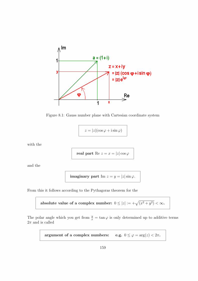
Figure 8.1: Gauss number plane with Cartesian coordinate system

z = |z|(cosϕ+ i sinϕ)

with the

real part Re z = x = |z| cosϕ

and the

imaginary part Im z = y = |z| sinϕ.

From this it follows according to the Pythagoras theorem for the

absolute value of a complex number: 0 ≤ |z| := +√

(x2 + y2) <∞.

The polar angle which you get from yx

= tanϕ is only determined up to additive terms2π and is called

argument of a complex numbers: e.g. 0 ≤ ϕ = arg(z) < 2π.

159

Determining the argument we come across a small difficulty, an ambiguity which occursbecause of y

x= −y−x :

When we for example look at the complex number a = 1+i with the real part Re a = 1 andthe imaginary part Im a = 1, we obtain, for the absolute value unambiguously |a| =

√2

for the argument, however, at first glance two values α = arg a = arctan 1 = π4

or 54π,

which both lie in the interval [0, 2π). By inserting both values in question in Re a wecan, however, find the right argument: for α = π

4we correctly find Re a = |a| cosα =√

2 cos π4

=√

2√2

= +1, while α = 54π gives us the wrong result Re a =

√2 cos 5

4π =

√2

−√

2=

−1.

Insert: Precise calculation of the arguments: For precise calculation

of the argument of a complex number from its real and imaginary part within our

chosen borders you can use the following equations:

for x > 0 and y ≥ 0 use ϕ = arg(x+ iy) = arctan yx ,

for x > 0 and y < 0 use ϕ = arg(x+ iy) = arctan yx + 2π,

for x < 0 and y arb. use ϕ = arg(x+ iy) = arctan yx + π,

for x = 0 and y > 0 use ϕ = arg(x+ iy) = π/2,

for x = 0 and y < 0 use ϕ = arg(x+ iy) = 3π/2 and

for x = 0 and y = 0 the argument is indeterminate.

Insert: Alternative choice of the borders of the arguments: Look-ing forward to future applications, many textbooks, computer programs and ISO- orDIN-standardization conventions choose for the arguments of the complex numbersinstead of the polar angle interval (you are accustomed to from school) an intervalof length 2π which is symmetrical around the real axis. They call these main ar-guments of a complex number and sometimes signify this choice by a capitalA: −π < ϕ = Arg(z) ≤ π.

In the case of these symmetrical borders you get the main argument of a complex

number from its real and imaginary part out of the following equations:

for x > 0 and y arb. out of ϕ = Arg(x+ iy) = arctan yx ,

for x < 0 and y ≥ 0 out of ϕ = Arg(x+ iy) = arctan yx + π,

for x < 0 and y < 0 out of ϕ = Arg(x+ iy) = arctan yx − π,

for x = 0 and y > 0 out of ϕ = Arg(x+ iy) = π/2,

for x = 0 and y < 0 out of ϕ = Arg(x+ iy) = −π/2 and

for x = 0 and y = 0 once more the main argument is indeterminate.

Exercise 8.2 Argument of a complex number:

Determine the argument of the complex number b = 1− i.

160

8.1.5 Euler’s Formula

When we insert for cosine and sine the Taylor series into the representation of complexnumbers in planar polar coordinates, we come across an interesting relation:

z

|z|= cosϕ+ i sinϕ

=∞∑n=0

(−1)nϕ2n

(2n)!+ i

∞∑n=0

(−1)nϕ2n+1

(2n+ 1)!If in this we insert the relation −1 = i2 we obtain:

=∞∑n=0

(i2)nϕ2n

(2n)!+ i

∞∑n=0

(i2)nϕ2n+1

(2n+ 1)!and contracted:

=∞∑n=0

(iϕ)2n

(2n)!+∞∑n=0

(iϕ)2n+1

(2n+ 1)!. Written out, we get:

= 1 +(iϕ)2

2!+

(iϕ)4

4!+

(iϕ)6

6!+ . . .+

(iϕ)

1!+

(iϕ)3

3!+

(iϕ)5

5!+

(iϕ)7

7!+ . . .

=∞∑n=0

(iϕ)n

n!.

This series looks familiar to us: We recognize the Taylor series which enabled us tocalculate the functional values of the exponential function. The difference is, an “i” is nowpreceding the real variable ϕ. Through this discovery we feel encouraged to define theexponential function for an imaginary variable through the above mentioned series:

exponential function for an imaginary variable: eiϕ :=∞∑n=0

(iϕ)n

n!.

With this definition the derived relation takes a very simple form, which has becomefamous as:

Euler’s formula: eiϕ := cosϕ+ i sinϕ.

From this, we extract Re eiϕ = cosϕ and Im eiϕ = sinϕ. Since cosine and sine are peri-odic functions with the period 2π, accordingly the exponential function of an imaginaryvariables must be a 2π-periodic function, too:

161

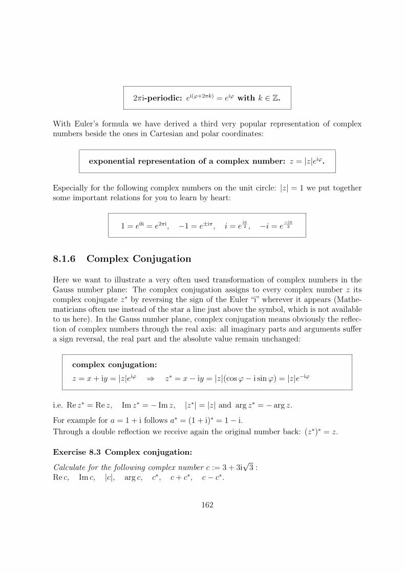
2πi-periodic: ei(ϕ+2πk) = eiϕ with k ∈ Z.

With Euler’s formula we have derived a third very popular representation of complexnumbers beside the ones in Cartesian and polar coordinates:

exponential representation of a complex number: z = |z|eiϕ.

Especially for the following complex numbers on the unit circle: |z| = 1 we put togethersome important relations for you to learn by heart:

1 = e0i = e2πi, −1 = e±iπ, i = eiπ2 , −i = e

−iπ2

8.1.6 Complex Conjugation

Here we want to illustrate a very often used transformation of complex numbers in theGauss number plane: The complex conjugation assigns to every complex number z itscomplex conjugate z∗ by reversing the sign of the Euler “i” wherever it appears (Mathe-maticians often use instead of the star a line just above the symbol, which is not availableto us here). In the Gauss number plane, complex conjugation means obviously the reflec-tion of complex numbers through the real axis: all imaginary parts and arguments suffera sign reversal, the real part and the absolute value remain unchanged:

complex conjugation:

z = x+ iy = |z|eiϕ ⇒ z∗ = x− iy = |z|(cosϕ− i sinϕ) = |z|e−iϕ

i.e. Re z∗ = Re z, Im z∗ = − Im z, |z∗| = |z| and arg z∗ = − arg z.

For example for a = 1 + i follows a∗ = (1 + i)∗ = 1− i.

Through a double reflection we receive again the original number back: (z∗)∗ = z.

Exercise 8.3 Complex conjugation:

Calculate for the following complex number c := 3 + 3i√

3 :Re c, Im c, |c|, arg c, c∗, c+ c∗, c− c∗.

162

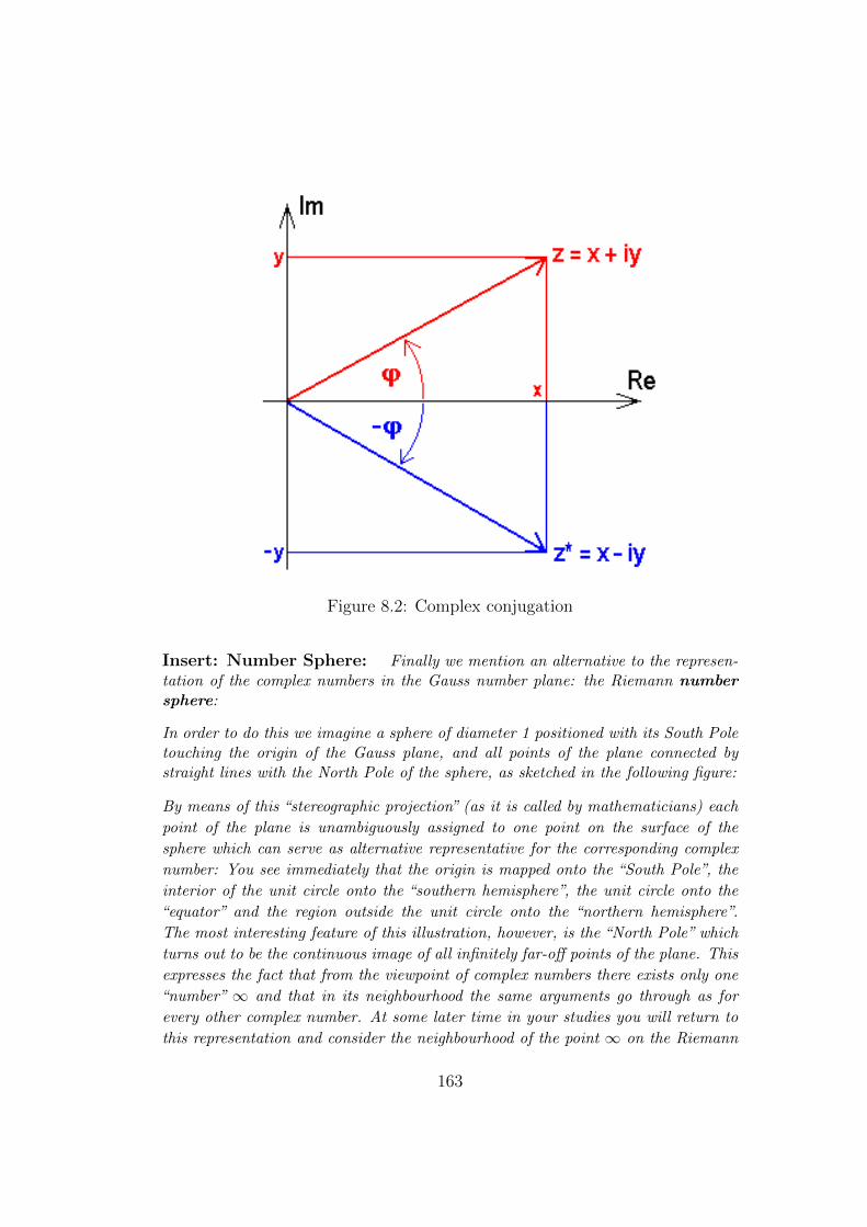
Figure 8.2: Complex conjugation

Insert: Number Sphere: Finally we mention an alternative to the represen-tation of the complex numbers in the Gauss number plane: the Riemann numbersphere:

In order to do this we imagine a sphere of diameter 1 positioned with its South Poletouching the origin of the Gauss plane, and all points of the plane connected bystraight lines with the North Pole of the sphere, as sketched in the following figure:

By means of this “stereographic projection” (as it is called by mathematicians) each

point of the plane is unambiguously assigned to one point on the surface of the

sphere which can serve as alternative representative for the corresponding complex

number: You see immediately that the origin is mapped onto the “South Pole”, the

interior of the unit circle onto the “southern hemisphere”, the unit circle onto the

“equator” and the region outside the unit circle onto the “northern hemisphere”.

The most interesting feature of this illustration, however, is the “North Pole” which

turns out to be the continuous image of all infinitely far-off points of the plane. This

expresses the fact that from the viewpoint of complex numbers there exists only one

“number” ∞ and that in its neighbourhood the same arguments go through as for

every other complex number. At some later time in your studies you will return to

this representation and consider the neighbourhood of the point ∞ on the Riemann

163

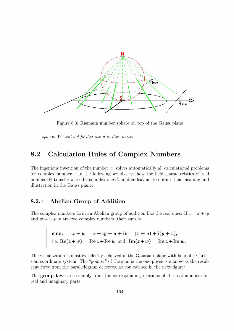
Figure 8.3: Riemann number sphere on top of the Gauss plane

sphere. We will not further use it in this course.

8.2 Calculation Rules of Complex Numbers

The ingenious invention of the number “i” solves automatically all calculational problemsfor complex numbers. In the following we observe how the field characteristics of realnumbers R transfer onto the complex ones C and endeavour to obtain their meaning andillustration in the Gauss plane:

8.2.1 Abelian Group of Addition

The complex numbers form an Abelian group of addition like the real ones: If z = x+ iyand w = u+ iv are two complex numbers, their sum is:

sum: z + w = x+ iy + u+ iv = (x+ u) + i(y + v),

i.e. Re(z+w) = Re z+Rew and Im(z+w) = Im z+Imw.

The visualization is most excellently achieved in the Gaussian plane with help of a Carte-sian coordinate system: The “pointer” of the sum is the one physicists know as the resul-tant force from the parallelogram of forces, as you can see in the next figure:

The group laws arise simply from the corresponding relations of the real numbers forreal and imaginary parts.

164

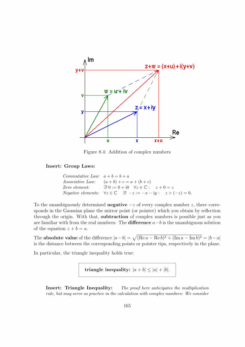
Figure 8.4: Addition of complex numbers

Insert: Group Laws:

Commutative Law: a+ b = b+ aAssociative Law: (a+ b) + c = a+ (b+ c)Zero element: ∃! 0 := 0 + i0 ∀z ∈ C : z + 0 = zNegative elements: ∀z ∈ C ∃! −z := −x− iy : z + (−z) = 0.

To the unambiguously determined negative −z of every complex number z, there corre-sponds in the Gaussian plane the mirror point (or pointer) which you obtain by reflectionthrough the origin. With that, subtraction of complex numbers is possible just as youare familiar with from the real numbers: The difference a−b is the unambiguous solutionof the equation z + b = a.

The absolute value of the difference |a−b| =√

(Re a− Re b)2 + (Im a− Im b)2 = |b−a|is the distance between the corresponding points or pointer tips, respectively in the plane.

In particular, the triangle inequality holds true:

triangle inequality: |a+ b| ≤ |a|+ |b|.

Insert: Triangle Inequality: The proof here anticipates the multiplicationrule, but may serve as practice in the calculation with complex numbers: We consider

165

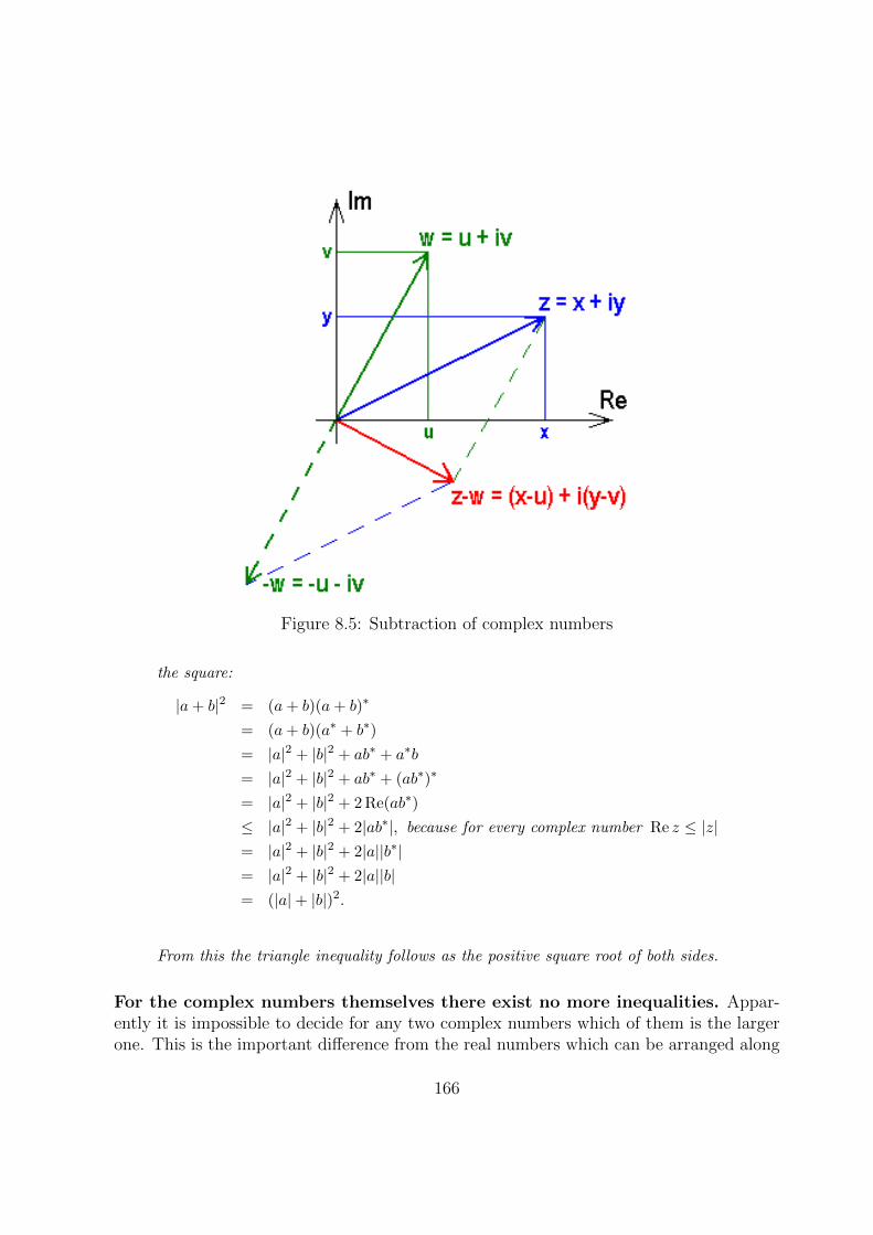
Figure 8.5: Subtraction of complex numbers

the square:

|a+ b|2 = (a+ b)(a+ b)∗

= (a+ b)(a∗ + b∗)

= |a|2 + |b|2 + ab∗ + a∗b

= |a|2 + |b|2 + ab∗ + (ab∗)∗

= |a|2 + |b|2 + 2 Re(ab∗)

≤ |a|2 + |b|2 + 2|ab∗|, because for every complex number Re z ≤ |z|= |a|2 + |b|2 + 2|a||b∗|= |a|2 + |b|2 + 2|a||b|= (|a|+ |b|)2.

From this the triangle inequality follows as the positive square root of both sides.

For the complex numbers themselves there exist no more inequalities. Appar-ently it is impossible to decide for any two complex numbers which of them is the largerone. This is the important difference from the real numbers which can be arranged along

166

the number line and the price we have to pay for the extension. There is however yet a“memory of ordering”, namely from a 6= b follows a+ c 6= b+ c just as before.

The complex conjugate of a sum is the sum of the conjugate summands:

(z + w)∗ = (z∗ + w∗)

meaning, the star can be drawn into the brackets. From the sum resp. difference of acomplex number and its complex conjugate we can easily obtain the real resp. imaginarypart:

Re z = z + z∗

2 resp. Im z = z − z∗2i .

The complex conjugate z∗ = |z|(cosϕ− i sinϕ) = |z|e−iϕ also allows us the reversal of theEuler formula:

cosϕ = z + z∗

2|z| and sinϕ = z − z∗2i|z| .

8.2.2 Abelian Group of Multiplication

Also for the multiplication rule Euler’s “i” regulates everything automatically. We cansimply multiply both the complex numbers z = x + iy and w = u + iv with each otherapplying the laws known from the real numbers and taking into account that i2 = −1:

zw = (x+ iy)(u+ iv) = xu+ i(yu+ xv) + i2yv = (xu− yv) + i(yu+ xv)

Thus, we get a fairly complicated expression for the

product: zw = (xu− yv) + i(yu+ xv).

167

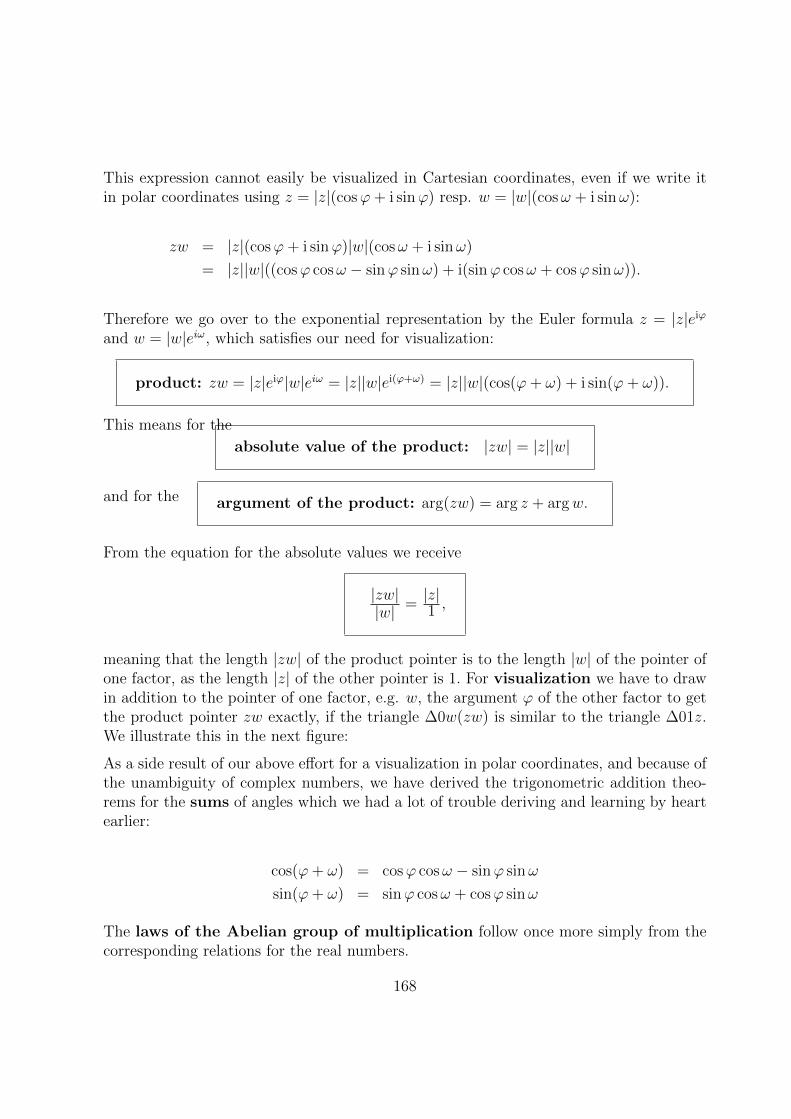
This expression cannot easily be visualized in Cartesian coordinates, even if we write itin polar coordinates using z = |z|(cosϕ+ i sinϕ) resp. w = |w|(cosω + i sinω):

zw = |z|(cosϕ+ i sinϕ)|w|(cosω + i sinω)

= |z||w|((cosϕ cosω − sinϕ sinω) + i(sinϕ cosω + cosϕ sinω)).

Therefore we go over to the exponential representation by the Euler formula z = |z|eiϕ

and w = |w|eiω, which satisfies our need for visualization:

product: zw = |z|eiϕ|w|eiω = |z||w|ei(ϕ+ω) = |z||w|(cos(ϕ+ ω) + i sin(ϕ+ ω)).

This means for the

absolute value of the product: |zw| = |z||w|

and for the argument of the product: arg(zw) = arg z + argw.

From the equation for the absolute values we receive

|zw||w| =

|z|1 ,

meaning that the length |zw| of the product pointer is to the length |w| of the pointer ofone factor, as the length |z| of the other pointer is 1. For visualization we have to drawin addition to the pointer of one factor, e.g. w, the argument ϕ of the other factor to getthe product pointer zw exactly, if the triangle ∆0w(zw) is similar to the triangle ∆01z.We illustrate this in the next figure:

As a side result of our above effort for a visualization in polar coordinates, and because ofthe unambiguity of complex numbers, we have derived the trigonometric addition theo-rems for the sums of angles which we had a lot of trouble deriving and learning by heartearlier:

cos(ϕ+ ω) = cosϕ cosω − sinϕ sinω

sin(ϕ+ ω) = sinϕ cosω + cosϕ sinω

The laws of the Abelian group of multiplication follow once more simply from thecorresponding relations for the real numbers.

168

Figure 8.6: Multiplication of complex numbers

Insert: Group Laws:

Commutative Law: ab = baAssociative Law: (ab)c = a(bc)Unity element: ∃! 1 := 1 + i0 ∀z ∈ C : 1 · z = zInverse elements: ∀z = reiϕ ∃!z−1 := r−1e−iϕ with z · z−1 = 1

The existence of an unambiguous inverse enables division by complex numbers: thequotient a · b−1 =: a

bsolves the equation z · b = a for b 6= 0. To visualize the quotient we

calculate

quotient: zw =

|z|eiϕ

|w|eiω =|z||w|e

i(ϕ−ω) =|z||w|(cos(ϕ− ω) + i sin(ϕ− ω)).

This means for the169

absolute value of the quotient:∣∣ zw∣∣ =|z||w|

and for theargument of the quotient: arg( z

w) = arg z − argw.

From the equation for the absolute values we get

| zw ||z| = 1

|w| ,

i.e. the length∣∣ zw

∣∣ of the quotient pointer is to the length |z| of the pointer of thenumerator, as 1 to the length |w| of the denominator. To get a good visualization wehave just to subtract the argument ω of the denominator from the argument ϕ of thenumerator z to get the quotient pointer z

wexactly, if the triangle ∆0( z

w)z is similar to the

triangle ∆01w. We have a look at this in more detail in the next figure:

170

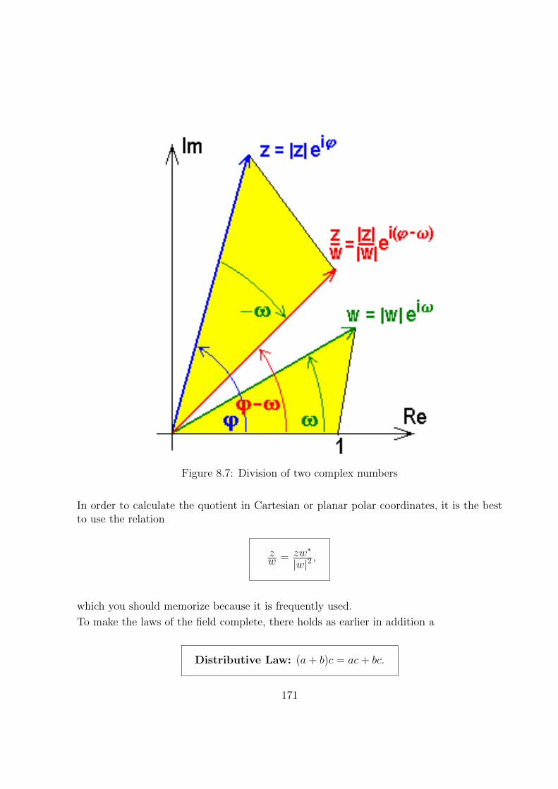
Figure 8.7: Division of two complex numbers

In order to calculate the quotient in Cartesian or planar polar coordinates, it is the bestto use the relation

zw = zw∗

|w|2 ,

which you should memorize because it is frequently used.

To make the laws of the field complete, there holds as earlier in addition a

Distributive Law: (a+ b)c = ac+ bc.

171

The complex conjugate of a product is the product of the conjugate of its factors:

(zw)∗ = z∗w∗.

The star may be drawn into the brackets as in the case of the sum.

In calculations with complex numbers an often-used fact is that the product of a complexnumber with its own complex conjugate is always a real number:

zz∗ = (x+ iy)(x− iy) = x2 + y2 = |z|2 ∈ R.

This relation may also be helpful, if you want to keep the denominator real: 1z = z∗

|z|2 .

Also in multiplication, there is a modest “memory” of the order which was lost in theextension of the real number into the complex ones: From a 6= b and c 6= 0 there followsac 6= bc.

Exercise 8.4 Multiplication and division of a complex number:

Calculate for the complex number c := 3 + 3i√

3 :cc∗, c2, c/c∗, 1/c, 1/c∗, 1/c+ 1/c∗, 1/c− 1/c∗ and c3.

Exercise 8.5 Multiplication and division of complex numbers:

Calculate for a general complex number z = reiϕ :zz∗, z2, z/z∗, |z/z∗|, 1/z + 1/z∗, 1/z − 1/z∗.

Exercise 8.6 Simple mappings:

Choose a complex number z and calculate for it: a) iz, b) 1/z and c) 1/z∗.

Exercise 8.7 Other product definitions:

Show by a counterexample that the “memory” of order mentioned above: a 6= b, c 6= 0⇒ ac 6= bc would not hold, if we had chosen the simpler definition a × b := a1b1 + ia2b2

instead of the one suggested by Euler’s “i”.

172

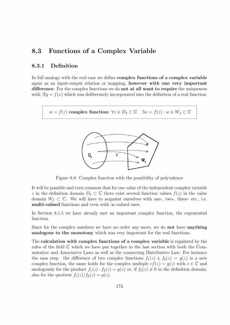
8.3 Functions of a Complex Variable

8.3.1 Definition

In full analogy with the real case we define complex functions of a complex variableagain as an input-output relation or mapping, however with one very importantdifference: For the complex functions we do not at all want to require the uniquenesswith ∃!y = f(x) which was deliberately incorporated into the definition of a real function:

w = f(z) complex function: ∀z ∈ Df ⊂ C ∃w = f(z) : w ∈ Wf ⊂ C

Figure 8.8: Complex function with the possibility of polyvalence

It will be possible and even common that for one value of the independent complex variablez in the definition domain Df ⊂ C there exist several function values f(z) in the valuedomain Wf ⊂ C. We will have to acquaint ourselves with one-, two-, three- etc., i.e.multi-valued functions and even with ∞-valued ones.

In Section 8.1.5 we have already met an important complex function, the exponentialfunction.

Since for the complex numbers we have no order any more, we do not have anythinganalogous to the monotony which was very important for the real functions.

The calculation with complex functions of a complex variable is regulated by therules of the field C which we have put together in the last section with both the Com-mutative and Associative Laws as well as the connecting Distributive Law: For instancethe sum resp. the difference of two complex functions f1(z) ± f2(z) = g(z) is a newcomplex function, the same holds for the complex multiple cf(z) = g(z) with c ∈ C andanalogously for the product f1(z) · f2(z) = g(z) or, if f2(z) 6= 0 in the definition domain,also for the quotient f1(z)/f2(z) = g(z).

173

8.3.2 Limits and Continuity

Also the transfer of the concept of the limit being central for real series and functionspresents no serious difficulties, since it was based on the distance between points whichwe have at our disposal also for complex numbers.

We say a sequence of complex numbers (zn)n∈N has a complex number z0 as limitand write: lim

n→∞zn = z0 (sometimes more casually: zn→∞ −→ z0), or call the sequence:

(zn)n∈N convergent to z0: ∃z0 : limn→∞

zn = z0 ⇐⇒∀ε > 0 ∃N(ε) ∈ N : |zn − z0| < ε ∀n > N(ε).

The last shorthand again means: for every pre-given tiny positive number ε a numberN(ε) can be found, such that the distance from the cluster point z0 for all members ofthe sequence with a larger number than N is smaller than the given tiny ε.

With this definition of the limit of complex numbers, all considerations about convergenceof complex numbers are reduced to the examination of the corresponding distances.

For complex functions we choose again a sequence (zn)n∈N ⊂ Df of complex numbers inthe definition domain Df of the function f, which for n→∞ tends to the number z0 ∈ Df .Then we calculate the function values at these points f(zn) which form a sequence again(f(xn))n∈N and check whether the sequence of these function values converges. If thiscan be shown for every sequence, out of the definition domain converging to z0, andalways with the same limit w0, we call the sequence of the function values convergent tow0 : lim

z→z0f(z) = w0 :

limz→z0

f(z) = w0 convergent: ⇐⇒ ∀(zn)n∈N : limn→∞

zn = z0 =⇒ limn→∞

f(zn) = w0

If we fill in our definition of the convergence of sequences, we receive:

limz→z0

f(z) = w0 convergent:

⇐⇒ ∀ε > 0 ∃δ > 0 : |f(z)− w0| < ε ∀z ∈ Df with |z − z0| < δ

To show this for all sequences is of course again easier said than done! We leave thisproblem to the mathematicians as earlier in the real number case and restrict ourselvesto some interesting cases which are clear anyway.

With this limit definition we can easily also define continuity for our complex functionsanalogously to our earlier definition:

174

w = f(z) continuous at x0 ⇐⇒ ∀ε > 0 ∃δ(ε) > 0 : |f(z)− w0| < ε ∀z with |z − z0| < δ

For limits this means again that at the considered point z0 the limit is given throughthe function value w0 = f(z0) of the limit z0 of a sequence (zn) in the definition domainof the argument: lim

z→z0f(z) = w0 = f(z0) = f( lim

n→∞zn). Visually this means that the

function f(z) maps pre-image points in the neighbourhood of z0 again in neighbouringimage points.

8.3.3 Graphic Illustration

Unfortunately, the graphic illustration of complex functions turns out to be significantlymore difficult than in the real case, since a complex function correlates four real quantities.Instead of mapping one real pre-image straight line, namely the x-axis, onto an other one,the image straight line or y-axis, we now have to map the complete pre-image complexplane, the z-plane, onto another one, the image or w-plane. In the graphic illustration of areal function of a real variable, we have become used to placing the pre-image and imagenumber lines orthogonal to one another and illustrating the mapping by means of a curvein this plane. For complex functions of a complex variable, we have to find new ways ofillustration. Mostly we will use the pre-image plane and the image plane drawn sideby side and characterize selected points or curves in the z-plane and their images in thew-plane by using the same symbols or colours.

Furthermore, a net of level curves of the real part u and imaginary part v over thez-plane or of the absolute value |w| and the argument arg w of the functionalvalues over an xy-net of the z-plane can give us a more exact idea of the mapping.

The best impression of the effect of a function we get through a perspective relief ofmountains for example with a xy-net over a certain range of the z-plane.

Because of these difficulties, we shall study only the most important functions chosenfrom our basis of real functions in the complex field:

8.3.4 Powers

First of all, as before, we consider the powers zn with natural exponents n ∈ N :

w = zn = (x+ iy)n = |z|n(cosϕ+ i sinϕ)n = |z|neinϕ = |z|n(cosnϕ+ i sinnϕ),

175

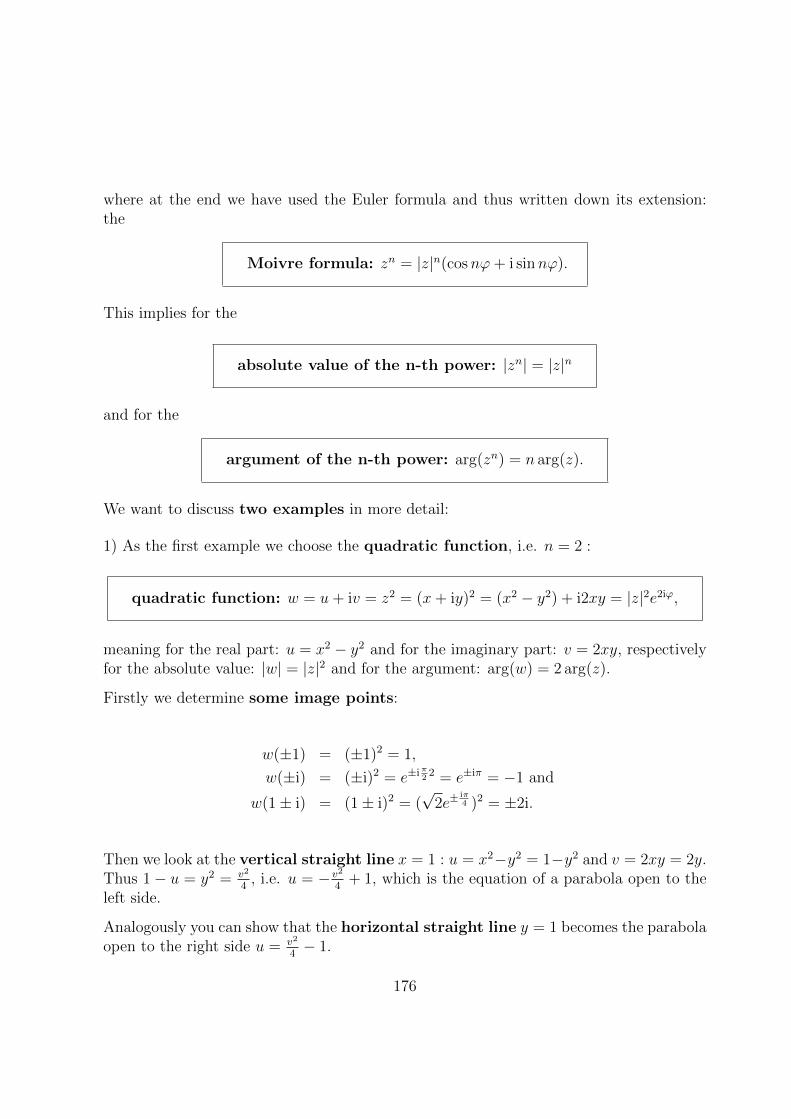
where at the end we have used the Euler formula and thus written down its extension:the

Moivre formula: zn = |z|n(cosnϕ+ i sinnϕ).

This implies for the

absolute value of the n-th power: |zn| = |z|n

and for the

argument of the n-th power: arg(zn) = n arg(z).

We want to discuss two examples in more detail:

1) As the first example we choose the quadratic function, i.e. n = 2 :

quadratic function: w = u+ iv = z2 = (x+ iy)2 = (x2 − y2) + i2xy = |z|2e2iϕ,

meaning for the real part: u = x2 − y2 and for the imaginary part: v = 2xy, respectivelyfor the absolute value: |w| = |z|2 and for the argument: arg(w) = 2 arg(z).

Firstly we determine some image points:

w(±1) = (±1)2 = 1,

w(±i) = (±i)2 = e±iπ2

2 = e±iπ = −1 and

w(1± i) = (1± i)2 = (√

2e±iπ4 )2 = ±2i.

Then we look at the vertical straight line x = 1 : u = x2−y2 = 1−y2 and v = 2xy = 2y.Thus 1− u = y2 = v2

4, i.e. u = −v2

4+ 1, which is the equation of a parabola open to the

left side.

Analogously you can show that the horizontal straight line y = 1 becomes the parabolaopen to the right side u = v2

4− 1.

176

Apparently the unit circle |z| = 1 is mapped onto itself by the quadratic function:|w| = 1.

From u = x2 − y2 = const. you can see that the hyperbolae with the bisectorsas asymptotes become vertical straight lines, and from v = 2xy = const., that thehyperbolae with the axes as asymptotes become horizontal straight lines.

The following figure gives an overview over the whole mapping. Note that the left-sidehalf of the pre-image plane is omitted, since the image of the right half alone coversthe entire w-plane.

Figure 8.9: Right half of the z-plane and the entire (upper) w-plane for the quadraticfunction

Insert: Rubber sheet: You can imagine the mapping procedure approximately

in the following way: think of the right-half of the z-plane as made of an elastic sheet

and then rotate the positive and negative halves of the imaginary axis in opposite

direction by 90 around the origin until they meet each other along the negative real

axis.

The image of the left half of the Gauss z-plane leads to a second cover of the whole w-plane. We already encountered part of this in connection with the real quadratic function,where the image of the negative pre-image half-axis covered the positive image half-axis asecond time, so that the square root function could only be defined over the positive half

177

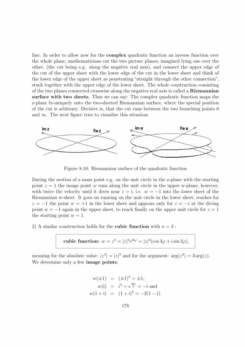
line. In order to allow now for the complex quadratic function an inverse function overthe whole plane, mathematicians cut the two picture planes, imagined lying one over theother, (the cut being e.g. along the negative real axis), and connect the upper edge ofthe cut of the upper sheet with the lower edge of the cut in the lower sheet and think ofthe lower edge of the upper sheet as penetrating “straight through the other connection”,stuck together with the upper edge of the lower sheet. The whole construction consistingof the two planes connected crosswise along the negative real axis is called a Riemanniansurface with two sheets. Thus we can say: The complex quadratic function maps thez-plane bi-uniquely onto the two-sheeted Riemannian surface, where the special positionof the cut is arbitrary. Decisive is, that the cut runs between the two branching points 0and ∞. The next figure tries to visualize this situation.

Figure 8.10: Riemannian surface of the quadratic function

During the motion of a mass point e.g. on the unit circle in the z-plane with the startingpoint z = 1 the image point w runs along the unit circle in the upper w-plane, however,with twice the velocity until it dives near z = i, i.e. w = −1 into the lower sheet of theRiemannian w-sheet. It goes on running on the unit circle in the lower sheet, reaches forz = −1 the point w = +1 in the lower sheet and appears only for z = −i at the divingpoint w = −1 again in the upper sheet, to reach finally on the upper unit circle for z = 1the starting point w = 1.

2) A similar construction holds for the cubic function with n = 3 :

cubic function: w = z3 = |z|3e3iϕ = |z|3(cos 3ϕ+ i sin 3ϕ),

meaning for the absolute value: |z3| = |z|3 and for the argument: arg(z3) = 3 arg(z).

We determine only a few image points:

w(±1) = (±1)3 = ±1,

w(i) = i3 = e3πi2 = −i and

w(1 + i) = (1 + i)3 = −2(1− i).

178

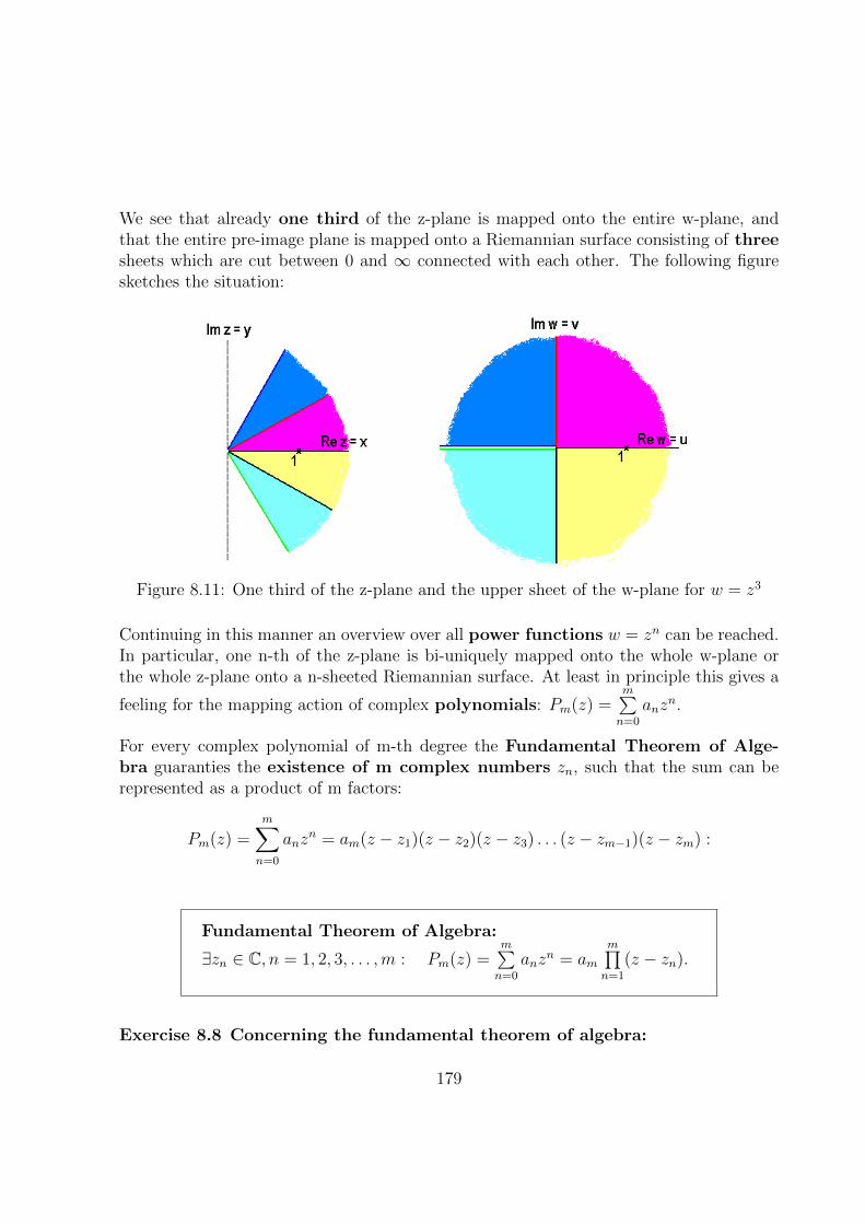
We see that already one third of the z-plane is mapped onto the entire w-plane, andthat the entire pre-image plane is mapped onto a Riemannian surface consisting of threesheets which are cut between 0 and ∞ connected with each other. The following figuresketches the situation:

Figure 8.11: One third of the z-plane and the upper sheet of the w-plane for w = z3

Continuing in this manner an overview over all power functions w = zn can be reached.In particular, one n-th of the z-plane is bi-uniquely mapped onto the whole w-plane orthe whole z-plane onto a n-sheeted Riemannian surface. At least in principle this gives a

feeling for the mapping action of complex polynomials: Pm(z) =m∑n=0

anzn.

For every complex polynomial of m-th degree the Fundamental Theorem of Alge-bra guaranties the existence of m complex numbers zn, such that the sum can berepresented as a product of m factors:

Pm(z) =m∑n=0

anzn = am(z − z1)(z − z2)(z − z3) . . . (z − zm−1)(z − zm) :

Fundamental Theorem of Algebra:

∃zn ∈ C, n = 1, 2, 3, . . . ,m : Pm(z) =m∑n=0

anzn = am

m∏n=1

(z − zn).

Exercise 8.8 Concerning the fundamental theorem of algebra:

179

Show with help of the Fundamental Theorem of Algebra, that the sum respectively the

product of the m zero points wn of a polynomial Pm(w) = 0 holds:m∑n=1

wn = −am−1am

respectivelym∏n=1

wn = (−1)m a0am .

For the complex infinite power series∞∑n=0

an(z − z0)n, the ones the mathematicians call

also “analytic functions”, we report without proof that all these series converge absolutelyinside a circle domain |z−z0| < R with the radius R around the development centre z0 anddiverge outside that region. Only now can we really understand the “convergence radius”R, that can be determined according to the criteria of convergence we have explained

earlier. For instance for the complex geometric series∞∑n=0

zn = 11−z the singularity at z = 1

restricts the radius of convergence to R = 1, as we have seen in Section 6.5 with help ofthe quotient criterion. Now we want to examine in more detail three very importantpower series as examples: the natural exponential function, which we already met, andthe complex sine and cosine functions.

8.3.5 Exponential Function

The most important complex function by far is the natural exponential function.Already in Section 8.1.5 through Euler’s formula we have been lead to its definition forpurely imaginary variables, and of course we can easily complete it for general complexvariables:

exponential function:

w = ez := exp(x+ iy) = exp(x)(cos y + i sin y) =∞∑n=0

zn

n!

i.e. for the absolute value:

|w| = |ez| = exp(Re z) = exp(x)

and for the argument:arg(w) = arg(ez) = Im z = y.

While the exponential function still rises rapidly as a function of its real part as we haveseen in the past, it is 2π-periodic in its dependence on the imaginary part of its variable.

180

2πi-periodic: ei(ϕ+2k) = eiϕ with k ∈ Z.

The convergence radius of the Taylor series is infinite as we have seen earlier.

The functional equation:

ezew = ez+wfor z, w ∈ C still holds true.

In order to visualize the function we first calculate once again some image points:w(1) = e,

w(0) = 1,

w(−1) =1

e,

w(iπ) = −1 and

w(iπ

2) = i.

Then we see that vertical straight lines Re z = x = const. are mapped into circles|w| = |ez| = eRe z = exp(x) = const.: the straight line x = 0 into the circle |w| = 1, theline x = 1 into the circle |w| = e and the straight line x = −1 into the circle |w| = 1

e.

The horizontal straight lines Im z = y = const. are mapped onto spokes argw =arg(ez) = Im z = const.: to be specific the straight line y = π onto the spoke argw = π,the line y = π

2onto argw = π

2, etc...

From these results we see that the exponential function maps a horizontal stripe of thez-plane with height 2π, for example the so-called fundamental area with −π < Im z ≤ πonto the w-plane which is cut open between the branching points 0 and ∞ (e.g. alongthe negative real axis). The entire z-plane therefore goes over into a Riemannian surfacewith infinitely many sheets. For each sheet the upper edge is continuously connectedalong the cut with the lower edge of the underlying sheet, and the upper edge of the lastsheet “through all other connections” with the lower edge of the first one. The followingfigure can help you to make a mental image of the effect of the function.


Having now studied the exponential function we will quickly take a look at the trigono-metric functions, cosine and sine, which we can easily derive with help of the Eulerformula from the exponential function, or define through their power series:

181

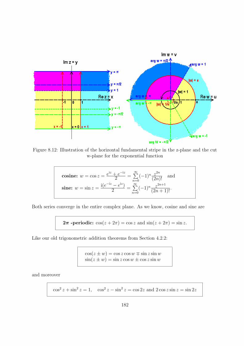
Figure 8.12: Illustration of the horizontal fundamental stripe in the z-plane and the cutw-plane for the exponential function

cosine: w = cos z = eiz + e−iz

2 =∞∑n=0

(−1)n z2n

(2n)!and

sine: w = sin z =i(e−iz − eiz)

2 =∞∑n=0

(−1)n z2n+1

(2n+ 1)!.

Both series converge in the entire complex plane. As we know, cosine and sine are

2π -periodic: cos(z + 2π) = cos z and sin(z + 2π) = sin z.

Like our old trigonometric addition theorems from Section 4.2.2:

cos(z ± w) = cos z cosw ∓ sin z sinwsin(z ± w) = sin z cosw ± cos z sinw

and moreover

cos2 z + sin2 z = 1, cos2 z − sin2 z = cos 2z and 2 cos z sin z = sin 2z

182

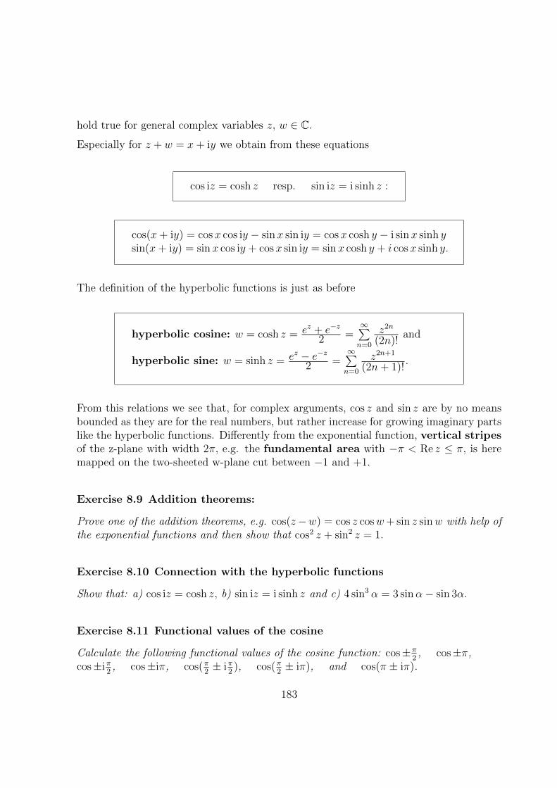
hold true for general complex variables z, w ∈ C.

Especially for z + w = x+ iy we obtain from these equations

cos iz = cosh z resp. sin iz = i sinh z :

cos(x+ iy) = cos x cos iy − sinx sin iy = cosx cosh y − i sinx sinh ysin(x+ iy) = sinx cos iy + cosx sin iy = sinx cosh y + i cosx sinh y.

The definition of the hyperbolic functions is just as before

hyperbolic cosine: w = cosh z = ez + e−z

2 =∞∑n=0

z2n

(2n)!and

hyperbolic sine: w = sinh z = ez − e−z2 =

∞∑n=0

z2n+1

(2n+ 1)!.

From this relations we see that, for complex arguments, cos z and sin z are by no meansbounded as they are for the real numbers, but rather increase for growing imaginary partslike the hyperbolic functions. Differently from the exponential function, vertical stripesof the z-plane with width 2π, e.g. the fundamental area with −π < Re z ≤ π, is heremapped on the two-sheeted w-plane cut between −1 and +1.

Exercise 8.9 Addition theorems:

Prove one of the addition theorems, e.g. cos(z−w) = cos z cosw+ sin z sinw with help ofthe exponential functions and then show that cos2 z + sin2 z = 1.

Exercise 8.10 Connection with the hyperbolic functions

Show that: a) cos iz = cosh z, b) sin iz = i sinh z and c) 4 sin3 α = 3 sinα− sin 3α.

Exercise 8.11 Functional values of the cosine

Calculate the following functional values of the cosine function: cos±π2, cos±π,

cos±iπ2, cos±iπ, cos(π

2± iπ

2), cos(π

2± iπ), and cos(π ± iπ).

183

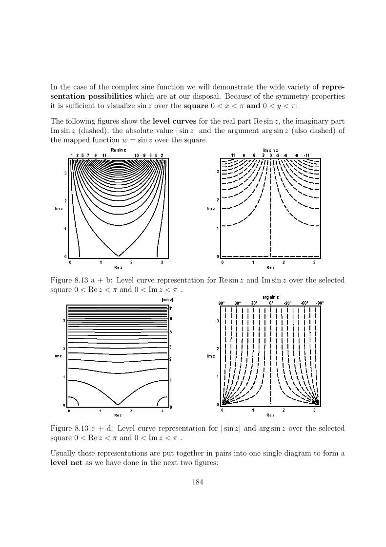
In the case of the complex sine function we will demonstrate the wide variety of repre-sentation possibilities which are at our disposal. Because of the symmetry propertiesit is sufficient to visualize sin z over the square 0 < x < π and 0 < y < π:

The following figures show the level curves for the real part Re sin z, the imaginary partIm sin z (dashed), the absolute value | sin z| and the argument arg sin z (also dashed) ofthe mapped function w = sin z over the square.

Figure 8.13 a + b: Level curve representation for Re sin z and Im sin z over the selectedsquare 0 < Re z < π and 0 < Im z < π .

Figure 8.13 c + d: Level curve representation for | sin z| and arg sin z over the selectedsquare 0 < Re z < π and 0 < Im z < π .

Usually these representations are put together in pairs into one single diagram to form alevel net as we have done in the next two figures:

184

Figure 8.13 e + f: Level net for Re sin z and Im sin z and resp. | sin z| and arg sin z overthe square

185

It requires some effort to get an impression of the represented function from the levelcurves of the image points. We succeed a little better if correlated with the mean valueof the function in that region, the areas between the curves are tinted in grey shadesover a scale which extends from deep black for small values to white for large values.This kind of representation is demonstrated by the Figures g) till j). Now, we can moreeasily imagine how the values of the imaginary part Im sin z with growing Im z one theone hand increase near Re z = 0 and on the other hand decrease near Re z = π. Also thetremendous increase of Re sin z and | sin z| with growing distance from the real axis showsup clearly.

Figure 8.13 g + h: Grey tinted level curve representation for Re sin z and Im sin z overthe square.

Figure 8.13 i + j:Grey tinted level curve representation for | sin z| and arg sin z over thesquare.

186

We achieve even more impressive pictures, if we use a colour scale to characterize therelative heights, for instance as done in geographical maps with their deep blue of thedeep oceans, different shades of green representing low lying land, the beige, and finally thedarker and darker browns of the mountains. In the computer program MATHEMATICAused here in the Figures k) till n) the colours of the rainbow are used to representfunction height according to the frequency of the light. (Magma-)Red colours representsmaller values and (sky-)blue colours stand for higher functional values. Through thesefigures we get a significant impression of the structure of the “function value mountains”.

Figure 8.13 k + l: Rain-bow-like coloured level curve representation for Re sin z andIm sin z over the square.

Figure 8.13 m + n: Rain-bow-like coloured level curve representation for | sin z| andarg sin z over the square.

187

In figure 8.13 n we see particularly well the linear increase of the phase from −90 atRe z = π to +90 at Re z = 0.

Also with this kind of representation, the coloured visualized level curves of a variablecan be upgraded to a net through the marking in of the (dashed) level curves of a secondvariable which however cannot yet be represented by colours. This fact is illustrated inthe next two figures:

Figure 8.13 o + p: Rain-bow-like coloured level net representation for Re sin z and Im sin zand resp. | sin z| and arg sin z over the square.

188

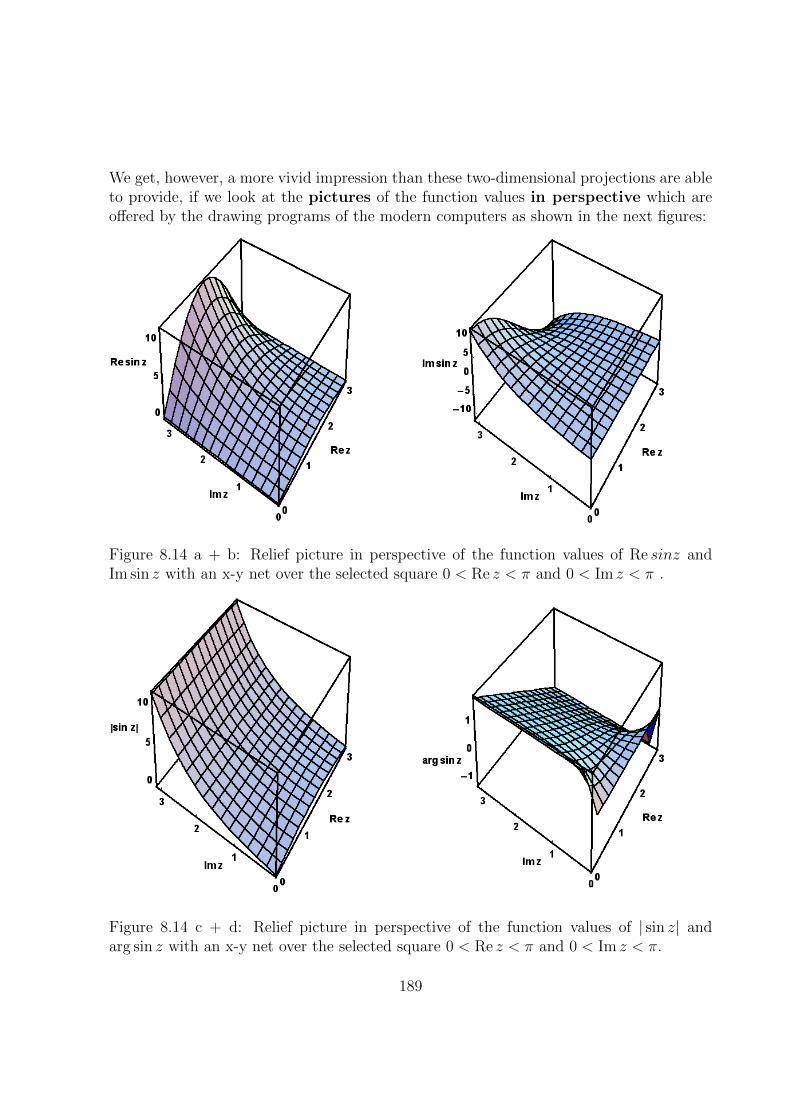
We get, however, a more vivid impression than these two-dimensional projections are ableto provide, if we look at the pictures of the function values in perspective which areoffered by the drawing programs of the modern computers as shown in the next figures:

Figure 8.14 a + b: Relief picture in perspective of the function values of Re sinz andIm sin z with an x-y net over the selected square 0 < Re z < π and 0 < Im z < π .

Figure 8.14 c + d: Relief picture in perspective of the function values of | sin z| andarg sin z with an x-y net over the selected square 0 < Re z < π and 0 < Im z < π.

189

To demonstrate the influence of the changes in sign, we have displayed for you finallythe four interesting variables with the help of the program MATHEMATICA over thelarger rectangle region 0 < Re z < π and −π < Im z < π, using revolving pictures:

Figure 8.15 a + b: Revolving relief picture in perspective of the function values of Re sinzand Im sin z with an x-y net over the selected rectangle region: 0 < Re z < π and−π < Im z < π.

Figure 8.15 c + d: Revolving relief picture in perspective of the function values of | sin z|and arg sin z with an x-y net over the selected rectangle region: 0 < Re z < π and−π < Im z < π.

190

If you view this valley along the positive imaginary axis, you will see clearly the realfunction | sin z| at a vertical cut over the real axis Im z = 0. Looking along the positivereal axis, you recognize the real function sinh y over the imaginary axis, and even thereal catenary function cosh y is visible as envelope above the straight line Re z = π

2.

After shifting the origin by π2

in direction of the real axis, these figures describe the reliefof the complex cosine function.

8.3.7 Roots

At the end of this chapter we take a look at some inverse functions in the complex field,where once again characteristic differences occur compared to the real case: First of allwe examine the root functions.

After having seen how the n-th power maps an n-th sector of the complex z-plane in thewhole w-plane, we expect inversely that the n-th root will map the whole z-plane in ann-th sector of the w-plane, meaning, it is an n-valued function, as we have admitted inthe complex field:

w = n√z = z

1n = (reiϕ)

1n = (rei(ϕ+2πk))

1n = n√re

i(ϕ+2πk)n for n ∈ N and k ∈ N0.

Here we have taken into consideration that e2πi = 1.

For the argument ϕ of the independent variable z there is the restriction (agreed to earlier)0 ≤ ϕ < 2π. But, for which non-negative integers k does the corresponding relation forthe argument of the image hold?

ϕ+ 2πk

n< 2π ⇐= k +

ϕ

2π< n⇐= k ≤ n− 1 < n− ϕ

2π, i.e. k = 0,1,2,3, ...,n− 1.

Thus there are exactly n n-th roots wk, which we shall label by the index k:

n n-th roots: wk = n√z = n√re

i(ϕ+2πk)n for n ∈ N.

The complex number w0 is called principal value. Furthermore we see that the n rootslie on a circle around the origin with radius n

√r at the corners of a regular n-polygon:

n−1∑k=0

wk = 0.

Exercise 8.12 Roots:

Prove thatn−1∑k=0

wk = 0 with the help of the result of Exercise 8.8.

191

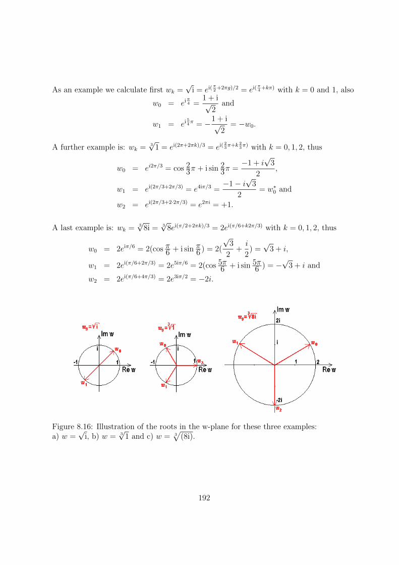
As an example we calculate first wk =√

i = ei(π2

+2πg)/2 = ei(π4

+kπ) with k = 0 and 1, also

w0 = eiπ4 =

1 + i√2

and

w1 = ei 54π = −1 + i√

2= −w0.

A further example is: wk = 3√

1 = ei(2π+2πk)/3 = ei( 23π+k 2

3π) with k = 0, 1, 2, thus

w0 = ei2π/3 = cos 23π + i sin 2

3π =−1 + i

√3

2,

w1 = ei(2π/3+2π/3) = e4iπ/3 =−1− i

√3

2= w∗0 and

w2 = ei(2π/3+2·2π/3) = e2πi = +1.

A last example is: wk = 3√

8i = 3√

8ei(π/2+2πk)/3 = 2ei(π/6+k2π/3) with k = 0, 1, 2, thus

w0 = 2eiπ/6 = 2(cos π6 + i sin π6 ) = 2(

√3

2+i

2) =√

3 + i,

w1 = 2ei(π/6+2π/3) = 2e5iπ/6 = 2(cos 5π6 + i sin 5π

6 ) = −√

3 + i and

w2 = 2ei(π/6+4π/3) = 2e3iπ/2 = −2i.

Figure 8.16: Illustration of the roots in the w-plane for these three examples:a) w =

√i, b) w = 3

√1 and c) w = 3

√(8i).

192

Exercise 8.13 Roots:

Calculate and sketch the following roots: a) w = 3√

i, b) w = 4√

(−1), c) w = 8√

1, d)

w = 4√−i and e) w = 2

√8i.

8.3.8 Logarithms

Finally we take a look at an infinitely multiple valued function, the natural

logarithm: w = ln z for z 6= 0.

Since the logarithm is the inverse function of the exponential function, the following hasto hold true:

z = |z|ei arg z = ew+2πik = eRew+i(Imw+2πk) with k ∈ Z

meaning, we have for the

real part of the logarithm: Re(ln z) = ln |z|

and the

imaginary part of the logarithm: Im(ln z) = arg z + 2πk with k ∈ Z

has infinitely many values, which differ by integer multiples of 2π. We choose for instancethe region −π < Im(Ln z) ≤ π as the principal value and write it with the capital letter:Ln, so that we obtain:

ln z = Ln z + 2πik with k ∈ Z

For example it follows

1) from e0 = 1 : Ln 1 = 0, thus ln 1 = 2πik,2) from eiπ = −1 : Ln(−1) = iπ, thus ln(−1) = iπ(1 + 2k)and3) from 3eiπ = −3 : Ln(−3) = ln | − 3|+ iπ, thus ln(−3) = 1.098 + iπ(1 + 2k).

Exercise 8.14 Logarithms:

Calculate ln i.

193

8.3.9 General Power

We need the logarithm here just as for the real field to define the general power function,which has therefore infinitely many values in the complex field:

General Power: w = bz := ez ln b, where ln b = ln |b|+ i(β + 2πg) with g ∈ Z,

since b = |b|ei(β+2πg).

As principal value of bz we take ez Ln b with the principal value Ln b of ln b. With this,we can for example calculate 1i: wg = 1i = ei ln 1 = ei2πig = e−2πg ∈ R :

w0 = 1, w1 = e−2π = 1.87 ·10−3, w2 = e−4π = 3.49 ·10−6, but also w−1 = e2π = 535.49,etc..

Surprisingly enough, even ii is real: wg = ii = ei ln i = ei·i(π/2+2πg) = e−(π/2+2πg) ∈ R :w0 = e−π/2 = 0.20788.

Exercise 8.15 Powers:

Calculate wg = ii for g = 1 and g = −1.

Exercise 8.16 Exponentiating:

When you have a free minute, realize that (ii)i has more different values than i(i·i).

After these curious jokes, we leave behind the complex numbers. During your studies,you will often return to these things, you will learn more complex functions, for examplethe group of broken linear functions: w = az+b

cz+d, whose mapping preserves angles and

circles. You will study and classify the different kinds of singularities as well as acquaintyourselves with the Laurent series as a generalization of the Taylor series. Particularly, ina mathematical lecture on complex analysis, you will investigate when complex functionsare differentiable (= analytic = holomorphic) and learn how you can calculate difficultreal integrals with help of the elegant residue theorem in the complex plane. We are surethat you will not be able to resist the charm and beauty of this mathematical theory, eventhough for science it is not really necessary, although very useful.

194

Chapter 9

VECTORS

9.1 Three-dimensional Euclidean Space

9.1.1 Three-dimensional Real Space

After we have dealt with functions of real variables and their analysis as well as with thesimplest arithmetic rules of complex numbers, we turn in the last chapter of this courseto the three-dimensional space in which we live and in which whole physics happens.

We all have a good visualization of three-dimensional space from our everyday experience.Typically we think of a room or a box with length, width and height in which one canplace three perpendicular rulers, one measuring length, one measuring width and oneheight. The position for instance of the upper right front corner of your keyboard canbe chosen to be the intersection point of the three rulers. Mathematicians constructthe three-dimensional real space R3 according to this model logically as an “outerproduct”of three real straight lines R1, as we have used them to illustrate the real numbers:R3 = R1

1 ⊗ R12 ⊗ R1

3.

9.1.2 Coordinate Systems

Physicists like to be able to characterize every point of the space exactly, and they usefor this purpose a coordinate system. To do so they first choose completely arbitrarily,but often very suitably one point of the space as zero, also called the origin. Throughthis point they lay once more completely arbitrarily three real straight lines and numberthem: R1

1,R12 and R1

3. This already defines a coordinate system. Nevertheless, usuallythey are a little more demanding and require that these three straight lines are pairwiseperpendicular to one another: R1

k ⊥ R1l for k, l = 1, 2, 3, yielding what is called a Carte-

sian coordinate system. If in addition the positive halfs of the three straight lines, now

195

called “coordinate axes”, are arranged or numbered such that the rotation of the posi-tive half of the 1-axis by an angle π/2 around the 3-axis into the positive half of the 2-axisis, when viewing along the direction of the positive 3-axis, a clockwise rotation (this isusually called a right-handed screw) then we have constructed the ideal, a (Cartesian)right handed coordinate system. To some of you this numbering of the axes is knownas right-hand rule because the positive halfs of the 1-, 2- and 3-axis are arranged likethumb, forefinger and middle finger of the spread right hand. In the following this kindof coordinate system should be always assumed.

Figure 9.1: “Right-handed screw”

On the positive half of each of the three coordinate axes R1k for k = 1, 2, 3 lies, in each case

once again completely arbitrarily chosen, the accompanying unit point Ek whose distancefrom zero fixes the length unit much as for a ruler. Thus every point P ∈ R3 of thethree-dimensional space can be labeled unambiguously by a coordinate triple of realnumbers P = (p1, p2, p3). The number pk is in each case the height above the coordinateplane spanned up by the other two real straight lines R1

l and R1m, measured in the unit

chosen by Ek.

9.1.3 Euclidean Space

Because we want to do measurements we need a measure of the distance between anytwo points P = (p1, p2, p3) and Q = (q1, q2, q3). Therefore, we introduce in the three-

196

Figure 9.2: Point with its coordinate triple

dimensional space a distance measure, namely according to Pythagoras the root of thesquares of the coordinate differences:

Distance: |PQ| =√

(q1 − p1)2 + (q2 − p2)2 + (q3 − p3)2

In particular, the distance of the point P from zero O is |PO| =√p2

1 + p22 + p2

3.

Exercise 9.1 Distances between points:

Calculate the distance between the points P = (2, 2, 4) and Q = (1,−2, 0) as well as thedistance of each point from zero.

Mathematicians call a space with this distance definition Euclidean. Then the distancebetween two different points P 6= Q is always positive |PQ| = |QP | > 0, and the distanceof a point from itself is zero: |PP | = 0. As usual the triangle inequality holds whichsays that in every triangle the sum of two side lengths is larger than the length of thethird side:

Triangle inequality: |PQ| ≤ |PR|+ |RQ|

197

Figure 9.3: Illustration of the triangle inequality

For two different distances |PQ| 6= |PR| between points P and Q or R, respectively, onenaturally can decide which is the larger one, because real numbers are involved which areordered on a straight line. The points of the space R3, however, can not be ordered, justas the complex numbers cannot.

9.1.4 Transformations of the Coordinate System

Hopefully you have noticed how arbitrarily we have proceeded with the choice of thecoordinate system. Because an intelligently chosen coordinate system can be extraordi-narily helpful for the daily work of physicists, the freedom in the choice of coordinates,however, and the independence of the results of physical measurements of this choice isof outstanding importance Therefore we want to discuss what would have happened hadwe made another choice:

In particular, four kinds of transformations of the coordinate system are of prac-tical interest. We select in each case a simple but typical example:

1. TRANSLATIONS (SHIFTS), e.g. by a distance of 1 cm in the 3-direction:

198

First the freedom in the choice of the origin attracts our attention: How would thecoordinates (p1, p2, p3) of the point P look, if we had chosen instead of the point O

another point, e.g., O = E3, as zero which is shifted by the distance |E3O| = 1 cmin the positive 3-direction?

Figure 9.4: Translation by the distance 1 cm in the positive 3-direction

From the figure we directly read off that for the numbers pk holds: p3 = p3 − 1,while p1 = p1 and p2 = p2 remain unchanged, thus all together:

(p1, p2, p3) = (p1, p2, p3 − 1).

Insert: Equals sign: Considering more carefully one finds that the well-known equals sign is used often with different meanings:

If we write 1/2 = 2/4 we mean “numerically equal”, i.e. the numericalvalues are identical after calculation. In this sense the equals sign is used in theequation (p1, p2, p3) = (p1, p2, p3−1): the numerical value of the first coordinatep1 of the point P in the shifted coordinate system S : p1 = p1 is equal to thenumber p1 of the 1-coordinate in the old system. Accordingly, the numericalvalue of the 3-coordinate in the shifted system p3 = p3 − 1 is smaller by 1 thanthe corresponding number in the old coordinate system.

199

If, however, we write P = (p1, p2, p3) we mean: the point P “is in the coor-dinate system S represented by” the three given coordinate numbers. Inthis equation it needs to be specified in which system the coordinates have beenmeasured. Usually one takes the point of view, this is signified by the symbolsfor the coordinates which remind us of the choice of our coordinate axes. Careis also needed if we want to represent the point in the shifted system. On no ac-count can we simply write P = (p1, p2, p3), because from this you could conclude(p1, p2, p3) = (p1, p2, p3) which is definitively wrong as we have seen.

There are obviously three ways out of this difficulty:

(a) Either we define a new sign for “is represented in the system ...by ...”,while we add a symbol for the coordinate system to the equals sign: pos-sibly “=” with the meaning “is represented in the system S by ...”, e.g.,P =(p1, p2, p3). But this is complicated and difficult to realize with com-puter fonts.

(b) Or we use the hat which labels the shifted coordinate system to also labelthe indices pk, e.g. pk, to remind us that the coordinates of the old point P

are now being given with respect to the new 1-, 2- or 3-axis of the systemS. This too is very difficult to realize on the computer, and moreoveruncommon.

(c) Therefore, we choose here the third possibility: We place the hat on thecoordinates, thus pk as done with alternative (a), avoiding, however, thestatement: “it is represented in the system S by ...” in equations.

Now that we have clarified this problem, there is no more reason for insecurity

or misunderstanding.

It is easy to generalize this result on translations to arbitrary distances and to otherdirections, so that we can skip this here.

Exercise 9.2 Point coordinates:

What are the coordinates of the point P in a coordinate system whose origin lies inthe point O = (1, 2,−3)?

Instead of this we now turn to other particularly important coordinate transforma-tions with which the origin remains unchanged: first to

2. ROTATIONS (TURNINGS), e.g. by the angle ϕ around the 3-direction:

We consider in addition to our original coordinate system S a new one S, whichwith unchanged origin O = O was rotated, e.g., by an angle ϕ around the 3-axisseen clockwise in the positive 3-direction:From the figure we see immediately that p1 = p1 cosϕ+ p2 sinϕ and p2 = p2 cosϕ−p1 sinϕ while p3 = p3, thus:

200

Figure 9.5: Rotation of the coordinate system by an angle ϕ around the 3-direction

(p1, p2, p3) = (p1 cosϕ+ p2 sinϕ, p2 cosϕ− p1 sinϕ, p3)

e.g., for: ϕ = π/2 : (p1, p2, p3) = (p2,−p1, p3).

Exercise 9.3 Rotated coordinate systems:

Calculate the coordinates of the point P in a coordinate system S which was rotatedaround the 3-direction relative to S by the angles ϕ = π, ϕ = π/4 or ϕ = π/6.

Further very interesting transformations which leave the origin invariant are the

3. REFLECTIONS (MIRRORINGS), e.g. through the origin (parity transforma-tion).

It is sufficient to consider just one reflection, because it is possible to constructall other reflections from this and suitable rotations. We choose the point reflec-tion through the origin which is illustrated in the following figure and is known byphysicists by the name parity transformation:We see immediately from the figure that all coordinates go over in their negative:

(p1, p2, p3) = (−p1,−p2,−p3)

201

Figure 9.6: Reflection of the coordinate system through the origin

Exercise 9.4 Reflections composed of parity and rotations:

Show how one can obtain the reflection in the 1-2-plane with ˆp1 = p1, ˆp2 = p2 andˆp3 = −p3 from the parity transformation and a rotation.

All reflections and especially the parity transformation have a remarkable propertywhich we easily recognize from the figure above: If we turn namely the positivehalf of the 1-axis by the angle π/2 into the positive half of the 2-axis, this is, seenin the direction of the positive 3-axis no more a right screw, but a left screw(anti-clockwise). Meaning: after a reflection a left coordinate system has becomefrom our right coordinate system. For people who have agreed on the use of rightcoordinate systems that is no pleasant situation, but we must learn to live with itand to find means and ways to detect also a hidden reflection always immediatelywhen we want to stay with right coordinate systems.

As the final example of transformations of the coordinate system we examine:

4. DILATATIONS (STRETCHINGS): especially of all three axes by a common fac-tor, e.g., 10:

Such a thing arises in practice when we want to measure lengths, instead of in cen-timeters cm, in decimeters dm. Under such a scale change the origin naturally

202

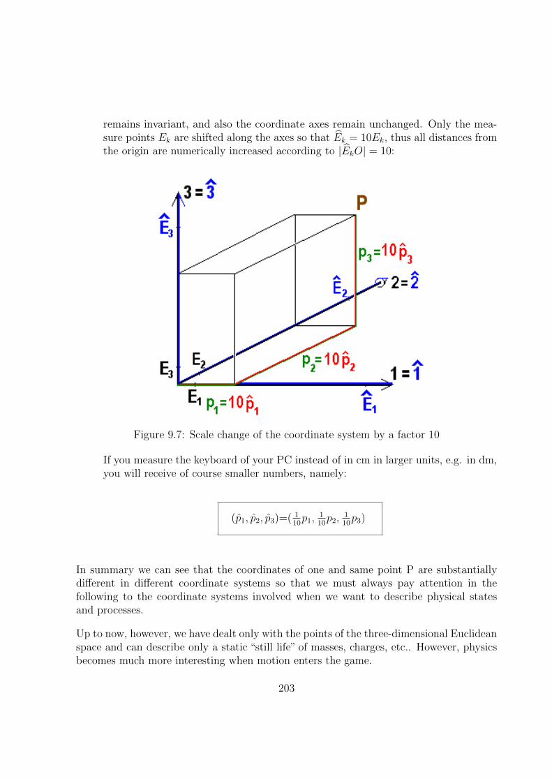
remains invariant, and also the coordinate axes remain unchanged. Only the mea-sure points Ek are shifted along the axes so that Ek = 10Ek, thus all distances fromthe origin are numerically increased according to |EkO| = 10:

Figure 9.7: Scale change of the coordinate system by a factor 10

If you measure the keyboard of your PC instead of in cm in larger units, e.g. in dm,you will receive of course smaller numbers, namely:

(p1, p2, p3)=( 110p1,

110p2,

110p3)

In summary we can see that the coordinates of one and same point P are substantiallydifferent in different coordinate systems so that we must always pay attention in thefollowing to the coordinate systems involved when we want to describe physical statesand processes.

Up to now, however, we have dealt only with the points of the three-dimensional Euclideanspace and can describe only a static “still life” of masses, charges, etc.. However, physicsbecomes much more interesting when motion enters the game.

203

9.2 Vectors as Displacements

9.2.1 Displacements

In the following we want to investigate what happens when we shift a mass point ora charge by a certain straight-line distance in a certain direction, e.g. from thestarting point P = (p1, p2, p3) to the final point Q = (q1, q2, q3) in a fixed arbitrarily chosencoordinate system. From a given starting point P with the three coordinates p1, p2 andp3 (three numbers!) a displacement by a given distance or length a (fourth number!)necessarily ends somewhere on the surface of a sphere with radius a around the startingpoint. In addition the direction of the displacement is fixed by two further numbers(!), e.g., the geographic longitude and latitude on the surface of the sphere or by twoother angles θ and ϕ. Thus all together we need six real numbers to fully represent adisplacement in three-dimensional space.

Such displacements, their causes and results are in many problems the central physicalentities, for instance displacement per unit time as velocity, or changes of velocity withtime as accelerations. By Newton’s Second Law, forces are proportional to accelerations,and therefore directly linked to displacements, consequently also forces per unit charge aselectric field strengths, etc...

When we look more exactly at typical physical examples, e.g. the velocity of a car ona straight section of a motorway, we find out that firstly the car consists of a lot ofpoints which have all identical velocity, and that secondly in most cases physics is notreally interested in the special starting values of all these points. The really importantinformation is the displacement common to all points of a body independent ofthe special starting or final points. When we take into account these physical requirementseconomically, we arrive at the concept of vectors:

9.2.2 Vectors

We call a displacement a vector ~a (or sometimes also a tensor of first order), if wesuppress the special starting and final position of a shifted object, if we are only interestedin the “displacement in itself”. In other words, only the amount of the distance of thedisplacement and the direction are interesting, and it does not matter where in the spacethe displacement takes place.

Because of the homogeneity of three-dimensional space, which is without exception pre-sumed in physics, this concept is advantageous for the formulation of universal validphysical laws. It means mathematically that, as for the introduction of the rationalnumbers where we have equated, e.g. 1/2 = 2/4 = 3/6 = ..., we divide displacements into

204

equivalence classes, and identify all displacements with the same distance amount anddirection. For illustration, we then can elect any representative of the class if necessary,for instance the so-called position vector, by applying the displacement to the origin.

After we have introduced a Cartesian coordinate system for the description of points bytheir coordinates in three-dimensional Euclidean space, the question rises how can wecharacterize the vectors in this system of three pairwise perpendicular coordinate axes.To do this we choose arbitrarily as representative of our vector ~a (marked by a small arrowabove the letter) a starting point P = (p1, p2, p3), shift this by the distance of the lengtha in the prescribed direction and reach thus the final point as in the following figure:

vector: ~a =−→PQ :=

q1 − p1

q2 − p2

q3 − p3

=

a1

a2

a3

(Except the small arrows used here above the Latin letter or above both points of therepresentative, other labels for vectors are underlined small letters, letters in boldfacetype or German letters.) In contrast to a certain special displacement of a certain pointwhich has to be labeled by six real numbers, a vector is characterized only by three realnumbers. In contrast to the three real “coordinates of a point” one calls these three realnumbers

vector components: ak = qk − pk.

Note that we also put them, like the point coordinates, in round brackets. To distinguishboth we write the components, however, usually (like above) as a column one belowanother instead of one after the other. If you want to have the vector components writtenlike the point coordinates one after the other, you should add an upper index “T”, as anabbreviation for “transposed”, i.e.:

transposed vector: aT = (a1, a2, a3).

As we can see from the figure, the three components of a vector are the lengths of the

three projections of the representative−→PQ on the coordinate axes or also the coordinates

of the final point A = (a1, a2, a3) which we reach by displacement if we have chosen theorigin as starting point. In this case we are using the position vector as representative:−→OA = (a1, a2, a3). By the use of these special representatives it becomes directly clearthat there is a reversibly unambiguous relation between the totality of the points of the

205

Figure 9.8: Vector components

R3 and the set of all vectors of the so-called vector space. Mathematicians call this anisomorphism.

Because a vector is unambiguously characterized by its three components, i.e. by thedistance amount and the two direction angles, a vector equation is equivalent tothree equations for the single components. For this reason vector notation can bea very efficient manner of writing:

vector equation: ~a = ~b ⇐⇒ ak = bk for k = 1, 2, 3.

The amount of the shift distance, i.e. the length of a vector, is determined fromits components according to Pythagoras, just as was the distance of two points fromcoordinate differences:

206

length:

a := |~a| = |PQ| =√

(q1 − p1)2 + (q2 − p2)2 + (q3 − p3)2

= |OA| =√a2

1 + a22 + a2

3.

Exercise 9.5 Lengths of vectors:

Determine the lengths of the following vectors:

304

and

−141

.

To make completely clear the typical differences (which exist in spite of the isomorphism)

between the components of a vector ~a =

(a1a2a3

)and the coordinates of the final point

A = (a1, a2, a3) of the representing position vector (to which the different manners ofwriting should remind us over and over again) we investigate once more what happens tothe vector components under transformations of the coordinate system:

9.2.3 Transformations of the Coordinate Systems

We want to investigate how the components ak of the fixed physically-given vector ~a =(a1a2a3

), possibly represented by

−→PQ, are changed if the coordinate system is subjected

to the four selected special transformations of Section 9.1.4 .

We start with the:

1. TRANSLATIONS (SHIFTS): e.g. by 1 in the 3-direction:

At first we are once again concerned with the arbitrariness of the choice of theorigin: How would the components of our vector look if we had instead of the pointO, selected as zero another point, e.g. O = E3 which is shifted by the distance|E3O| = 1 cm in the positive 3-direction? With the help of our results from 9.1.4.1we get:

a1

a2

a3

=

q1 − p1

q2 − p2

q3 − p3

=

q1 − p1

q2 − p2

q3 − p3

=

a1

a2

a3

.

207

Since the translation terms of the starting and end points of the representative cancelin the difference, we obtain (as expected because of the free mobility in the vectordefinition) the translational invariance of vectors, i.e. the arbitrary choice ofthe origin of our coordinate system has no consequences for the vector components.

From this also the length of the vectors is a translation invariant quantity:

a =√a2

1 + a22 + a2

3 =√a2

1 + a22 + a2

3 = a.

However, not all vector-like quantities in physics are translation invariant and not inevery physical problem, e.g., the forces acting on a rigid body away from the centreof mass, or also the field strength of an inhomogeneous electric field. Physicistsspeak then of bound vectors. In such cases, before the application of the vectoralgebra which we will develop in the next sections, we have to consider in each caseseparately to what extent the achieved results can be applied.

As the second example we examine

2. ROTATIONS (TURNINGS), e.g. by an angle ϕ around the 3-direction:

Keeping the origin O = O fixed we consider once more in addition to our oldcoordinate system S as in Figure 9.5 a new one: S which was rotated e.g. by anangle ϕ around the 3-axis seen clockwise in the positive 3-direction and we get (for

instance with the representative ~a =−→OA):

a1 = a1 cosϕ+ a2 sinϕ, a2 = a2 cosϕ− a1 sinϕ, a3 = a3.

For the rule according to which the new coordinates can be calculated from the oldones, mathematics offers a formulation which is known to most of you from school:the matrix formulation:

In order to get it, we write the three transformation equations one below the otherand complete the display with zeros in the following manner:

a1= a1 cosϕ +a2 sinϕ+a30a2=−a1 sinϕ+a2 cosϕ+a30a3= a10 + a20 +a31.

The factors necessary to get the new components ak from the old ones al are sum-marized by the following (3x3)-matrix D(3)(ϕ):

rotation matrix : D(3)(ϕ) :=

cosϕ sinϕ 0− sinϕ cosϕ 0

0 0 1

208

with the matrix elements D(3)zs (ϕ) for z, s = 1, 2, 3, where the index z marks the

(horizontal) lines (German: Zeilen) and s the (vertical) columns (German: Spalten).For example,

D(3)11 (ϕ) = D

(3)22 (ϕ) = cosϕ and

D(3)12 (ϕ) = −D(3)

21 (ϕ) = sinϕ, since the 1-2-plane is rotated,

D(3)33 (ϕ) = 1 to signalize that the 3-axis remains unchanged, and

D(3)13 (ϕ) = D

(3)31 (ϕ) = D

(3)23 (ϕ) = D

(3)32 (ϕ) = 0.

If instead of the single matrix elements D(3)zs (ϕ) we mean the entire matrix with

its nine elements, we use a bold capital letter D(3)(ϕ). The three equations forthe calculation of the new coordinates from the old ones is obtained in this newformulation through the following prescription of a generalized multiplicationrule for z = 1, 2, 3 :

az = D(3)z1 (ϕ)a1 +D

(3)z2 (ϕ)a2 +D

(3)z3 (ϕ)a3 =

3∑s=1

D(3)zs (ϕ)as =: D(3)

zs (ϕ)as.

In the last term the convenient Einstein summation convention was used. Thisallows us to omit the sum symbol whenever two identical indices (here the twoindices s) appear and in this way to signal the summation even without using theexplicit sum symbol.

According to this prescription we get the column vector of the components in therotated coordinate system by “multiplying” the column vector of the components inthe old system from the left by the rotation matrix: a1

a2

a3

=

cosϕ sinϕ 0− sinϕ cosϕ 0

0 0 1

a1

a2

a3

= D(3)(ϕ)

a1

a2

a3

To do this we imagine most simply the column vector transposed and pushed lineby line over the rotation matrix, multiply the terms lying on top of each other andadd up the three products.

Exercise 9.6 Special vectors in the rotated coordinate system

What are the components of the vectors ~a =

(111

), ~b =

(0−23

)and ~c =

(321

)in

a coordinate system S which was rotated with respect to the original system S byπ, π/2 or π/4 around the 3-direction?

209

Exercise 9.7 Change of the vector components by special rotations of thecoordinate system:

How are the components ak of a vector ~a changed, if we rotate the coordinate systemby the angle π or π/2 around the 3-axis?

In the matrix formulation the transformation equations can be most easily memo-rized: The number 1 occupies the position D

(3)33 (ϕ) because the 3-axis as the rotation

axis remains unchanged during the rotation and the 1-2 plane is rotated by ϕ. Alsothe extension to rotations around the two other axes can be imagined easily: e.g.for a rotation D(1)(ϕ) by ϕ around the 1-axis the matrix element must certainly be

D(1)11 (ϕ) = 1 and the 2-3-plane is rotated:

D(1)(ϕ) :=

1 0 00 cosϕ sinϕ0 − sinϕ cosϕ

meaning that a1 = a1, a2 = a2 cosϕ+ a3 sinϕ and a3 = a3 cosϕ− a2 sinϕ.

Exercise 9.8 Rotations around the 2-axis:

Realize through a sketch like our Figure 9.5 above that the coordinates of a pointA and consequently also the components of a vector ~a transform according to thefollowing rotation matrix in case of a rotation around the 2-axis.

D(2)(ϕ) :=

cosϕ 0 − sinϕ0 1 0

sinϕ 0 cosϕ

meaning that a3 = a3 cosϕ+ a1 sinϕ and a1 = a1 cosϕ− a3 sinϕ.

From this exercise you can find the transformation formulae for the three rotationsfrom each other without much calculation simply by replacing the indices cyclically(i.e. in a circle), meaning 1 by 2, 2 by 3 and 3 by 1:

Exercise 9.9 Special rotation matrices:

Determine the following rotation matrices: D(1)(π/2),D(1)(π/6) and D(2)(π/4).

The transformation formula for the components of a vector with rotations of thecoordinate system is an important characteristic feature of vectors, and sometimesvectors are simply defined as quantities whose three components transform with ro-tations of the coordinate system in the given manner. Indeed, when a physicist wantsto find out whether a quantity having three components is a vector, he measures

210

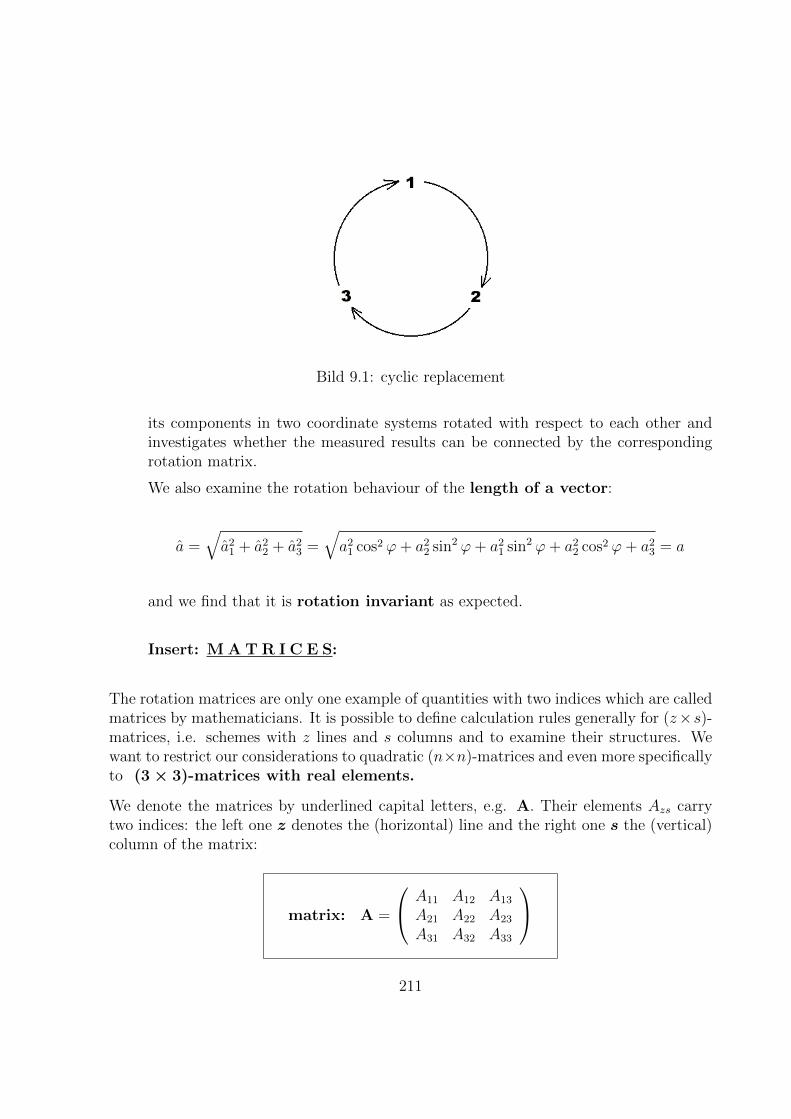
Bild 9.1: cyclic replacement

its components in two coordinate systems rotated with respect to each other andinvestigates whether the measured results can be connected by the correspondingrotation matrix.

We also examine the rotation behaviour of the length of a vector:

a =√a2

1 + a22 + a2

3 =√a2

1 cos2 ϕ+ a22 sin2 ϕ+ a2

1 sin2 ϕ+ a22 cos2 ϕ+ a2

3 = a

and we find that it is rotation invariant as expected.

Insert: M A T R I C E S:

The rotation matrices are only one example of quantities with two indices which are calledmatrices by mathematicians. It is possible to define calculation rules generally for (z×s)-matrices, i.e. schemes with z lines and s columns and to examine their structures. Wewant to restrict our considerations to quadratic (n×n)-matrices and even more specificallyto (3× 3)-matrices with real elements.

We denote the matrices by underlined capital letters, e.g. A. Their elements Azs carrytwo indices: the left one z denotes the (horizontal) line and the right one s the (vertical)column of the matrix:

matrix: A =

A11 A12 A13

A21 A22 A23

A31 A32 A33

211

Some kinds of matrices have special names because of their importance:In particular, diagonal matrices are of special importance, having only the three ele-ments A11, A22 and A33 along the so-called main diagonal (:from the left on top down-ward to the right) different from 0. The second diagonal (:from the right up downwardto the left) is, in comparison, much less important.

diagonal matrix: A =

A11 0 00 A22 00 0 A33

The matrices of rotations by a multiple of π are examples of diagonal matrices: D(1)(π),D(2)(π)and D(3)(π).

Half the way to the diagonal structure the triangle form is worth mentioning, which hasonly zeros either above or below the main diagonal:

triangle matrix: A =

A11 A12 A13

0 A22 A23

0 0 A33

Also matrices in box form are especially convenient for many purposes. In thesematrices non-zero elements are only in “boxes” around the main diagonal. Our rotationmatrices D(1)(ϕ) and D(3)(ϕ) are of this kind.

matrix in box form: A =

A11 A12 0A21 A22 00 0 A33

A simple operation that can be carried out with every matrix is transposition: Thismeans the reflection of all matrix elements through the main diagonal, or in other words,the exchange of lines and columns: ATzs = Asz

transposed matrix: AT =

A11 A21 A31

A12 A22 A32

A13 A23 A33

212

There exist matrices for which transposition does not change anything: They are calledsymmetric.

symmetric matrix: A = AT =

A11 A12 A13

A12 A22 A23

A13 A23 A33

These symmetric matrices occur very often in physics and have the advantage that theycan be brought to diagonal form by certain simple transformations.

As you see immediately, each symmetric matrix has only six independent elements.

If the reflection through the main diagonal leads to a minus sign, the matrix is calledantisymmetric:

antisymmetric matrix: A =

0 A12 A13

−A12 0 A23

−A13 −A23 0

Of course the diagonal elements have to vanish in this case. Apparently an antisymmetric(3 × 3)-matrix has only three independent elements. That is the deeper reason for theexistence of a vector product in three dimensions, as we will soon see in more detail.

Finally we mention a special quantity of every quadratic matrix: The sum of theelements along the main diagonal is called the trace (:in German “Spur”) of thematrix:

trace: Sp A = tr A =∑3

k=1Akk ≡ Akk

You can easily imagine that a termwise addition can be defined for the set of real (3 ×3)-matrices and that these form an Abelian group of addition with Associative Law,unique zero-matrix, exactly one negative for every matrix and Commutative Law, sincethe corresponding properties of the real numbers can simply be transferred to this newsituation. Also the termwise multiplication with a numerical factor is possible andleads to the usual Distributive Laws.

Much more important for physics is however the multiplication of two (3×3)-matriceswhich corresponds in the case of transformation matrices to two transformations of thecoordinate system carried out one after the other:

The following multiplicative instruction holds:

213

matrix multiplication: C = B A ⇐⇒ Czs :=∑3

k=1 BzkAks ≡ BzkAks

In the last part above the summation symbol is omitted according to the Einstein sum-mation convention, since the two identical indices signalize the summation well enough.

To calculate the product matrix element Czs in the z-th line and the s-th column youmay imagine the s-th (vertical) column Ams of the factor matrix A on the right side puthorizontally upon the z-th line Bzm of the left factor matrix B, elements on top of eachother multiplied and the three products added: e.g. C12 =

∑3k=1BzkAks ≡ BzkAks =

B11A12 +B12A22 +B13A32, thus altogether: B11 B12 B13

B21 B22 B23

B31 B32 B33

A11 A12 A13

A21 A22 A23

A31 A32 A33

)

=

B1kAk1 B1kAk2 B1kAk3



Exercise 9.10 Matrix multiplication:

Multiply the following transformation matrices:a) D(1)(θ)D(3)(ϕ) and compare with D(3)(ϕ)D(1)(θ),b) especially D(1)(π)D(3)(π/2) to be compared with D(3)(π/2)D(1)(π),c) D(3)(θ)D(3)(ϕ) and compare with D(3)(ϕ)D(3)(θ),d) D(1)(π)D(3)(π) and compare with D(3)(π)D(1)(π).

The most important discovery to be made by working through the Exercise 9.10 is thefact that generally no commutative law holds for rotations, and consequently not forthe representing matrices. You can easily check this visually with every match box as isillustrated in the following Figure:

The examples from Exercise 9.10 have already shown to you that in some exceptionalcases the commutative law nevertheless holds: all rotations around one and the sameaxis are for instance commutable. Also all diagonal matrices are commutable with eachother. This is the reason for their popularity. If A B 6= B A, the so-called commutationrelation [A,B] := A B − B A promises to be an interesting quantity. This will acquiregreat significance in quantum mechanics later on.

Apart from commutability, matrix multiplication behaves as expected: There holds an

Associative Law: C(B A) = C B A = (C B)A.

214

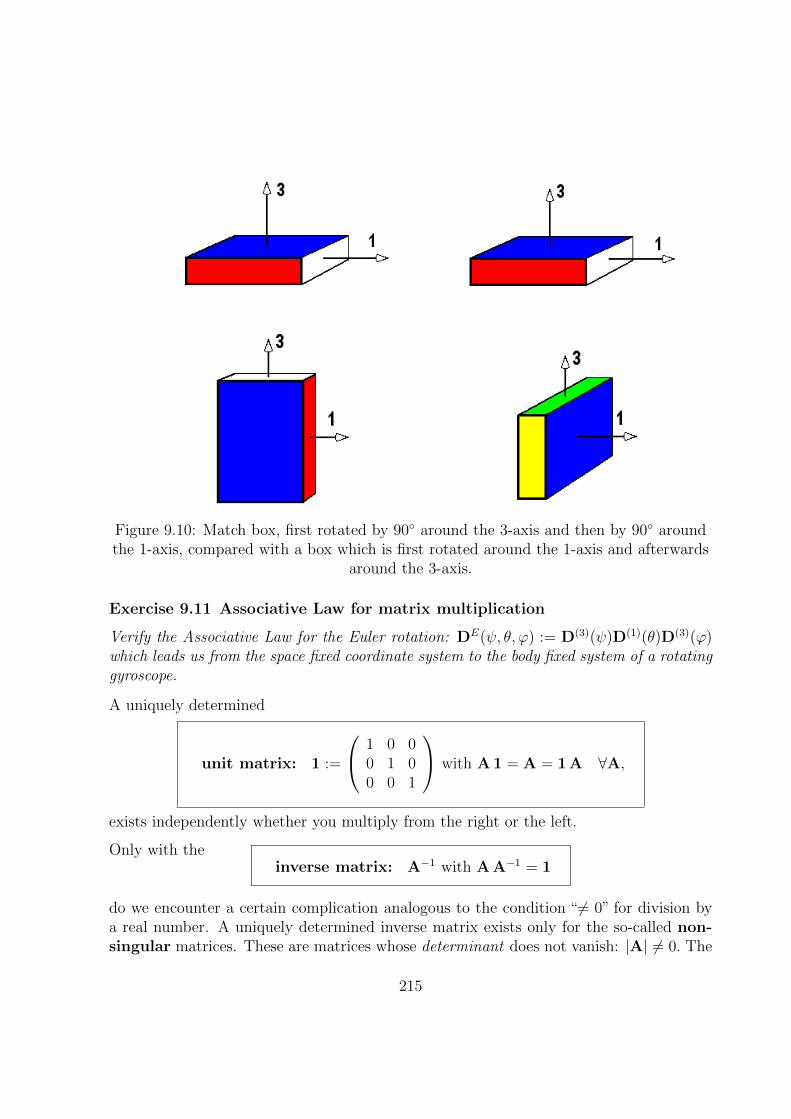
Figure 9.10: Match box, first rotated by 90 around the 3-axis and then by 90 aroundthe 1-axis, compared with a box which is first rotated around the 1-axis and afterwards

around the 3-axis.

Exercise 9.11 Associative Law for matrix multiplication

Verify the Associative Law for the Euler rotation: DE(ψ, θ, ϕ) := D(3)(ψ)D(1)(θ)D(3)(ϕ)which leads us from the space fixed coordinate system to the body fixed system of a rotatinggyroscope.

A uniquely determined

unit matrix: 1 :=

1 0 00 1 00 0 1

with A 1 = A = 1 A ∀A,

exists independently whether you multiply from the right or the left.

Only with theinverse matrix: A−1 with A A−1 = 1

do we encounter a certain complication analogous to the condition “6= 0” for division bya real number. A uniquely determined inverse matrix exists only for the so-called non-singular matrices. These are matrices whose determinant does not vanish: |A| 6= 0. The

215

determinants, the most important characteristics of matrices, will be treated in an extrainsert in the following subsection.

For our transformation matrices, however, this constraint is unimportant. For these ma-trices the inverse is simply the transposed one A−1 = AT which exists in every case aswe have seen: Mathematicians call these matrices orthogonal and we will inspect thesecarefully later on:

orthogonal matrix: A−1 = AT or A AT = 1

As our next transformation of the coordinate system we treat the:

3. REFLECTIONS (MIRRORINGS), e.g. through the origin (the parity transfor-mation).

We consider once more only the parity transformation, i.e. the reflection throughthe origin which transfers all coordinates and consequently all components into theirnegatives: Also this transformation which trivially leaves the origin invariant O = Omay be described by a matrix P, namely by the negative of the unit matrix whichwe denote by 1: P = −1

parity: P :=

−1 0 00 −1 00 0 −1

Thus we obtain for the components of a vector in the reflected system:

a1

a2

a3

=

−1 0 00 −1 00 0 −1

a1

a2

a3

= P

a1

a2

a3

=

−a1

−a2

−a3

All vectors whose components ak = −ak change sign through a reflection in theorigin are called polar vectors. Again not all vectors important in physics havethis property. We will soon come to physical vectors, e.g. the angular momentum,which are parity invariant. We will call these vectors axial vectors.

Nevertheless, for all kinds of vectors the length is parity invariant, because inevery case holds

a =√a2

1 + a22 + a2

3 =√a2

1 + a22 + a2

3 = a.

216

Insert: D E T E R M I N A N T S:

The most important characteristic of a matrix is its determinant. The following notationsare used:

determinant: det A ≡ |A| =

∣∣∣∣∣∣A11 A12 A13

A21 A22 A23

A31 A32 A33

∣∣∣∣∣∣Leibniz gave the following

definition of the determinant:

det A :=∑

(P1,P2,P3)

(−1)σ(P1,P2,P3)A1 P1A2 P2A3 P3 =

= A11A22A33 + A12A23A31 + A13A21A32

− A11A23A32 − A12A21A33 − A13A22A31.

This yields a real number, namely the sum resp. the difference of terms, each of which isa product of three matrix elements. The line indices (on the left hand) are always z = 123for all terms, while the column indices (on the right hand) go through all permutationsPz of these three numbers: (P1, P2, P3) = 123, 231, 312; 132, 213, 321. The sign of eachterm is fixed by the number of transpositions (:interchanges of each two indices) whichare needed to get the concerned configuration from the configuration 123. The first threeof the configurations above can be obtained by an even number of transpositions. Theyget a plus sign, the remaining three, obtained by an odd number of interchanges, weresubtracted: e.g. into 132 (odd), but 231 into 312 (even),.... In the case of (3×3)-matriceswe get six summands for which the even permutations can also be found through cyclicpermutation.

Besides these generally valid definitions there exist several different methods for the cal-culation of the determinant of a matrix. Here we will get to know two of them: first weconsider the Sarrus rule valid in particular for (3× 3)-matrices:

To get it we write the first and second column once more on the right beside to thedeterminant of interest:

to the Sarrus rule:

∣∣∣∣∣∣A11 A12 A13

A21 A22 A23

A31 A32 A33

∣∣∣∣∣∣A11 A12

A21 A22

A31 A32

217

Within this scheme we multiply the elements in the main diagonal A11A22A33 with eachother. To this product we add the product of the three elements standing next to the rightside in direction of the main diagonal +A12A23A31 and +A13A21A32. From this result wesubtract the product of the elements in the secondary diagonal −A11A23A32 and once moretwo times the products of the three matrix elements next to the right side in direction ofthe secondary diagonal −A12A21A33 and −A13A22A31. This procedure yields the desireddeterminant.

Very often a further method leads to the answer more quickly, the so-called developmentwith respect to the first line: Since this is an iterative method, we first note thatthe determinant of a (2× 2)-matrix consists of the product of the two diagonal elementsA11A22 diminished by the product of the two elements in the secondary diagonal −A12A21.Exactly this (2 × 2)-determinant is left over after removing both the third line and thethird column from our desired (3×3)-determinant. It is called adjoint and characterizedthrough the indices of the removed rows:

adjoint: adj33(A) = A11A22 − A12A21.

With help of these adjoints the desired (3×3) -determinant can be written in the followingway:

|A| = (−1)1+1A11 adj11(A) + (−1)1+2A12 adj12(A) + (−1)1+3A13 adj13(A)

=A11(A22A33 − A23A32)− A12(A21A33 − A23A31) + A13(A21A32 − A22A31).

We can see immediately that the restriction to the development with respect to the firstline means no limitation, since the determinant has many symmetry properties. Withhelp of those we can easily get developments with respect to other lines or columns. Herewe use the term

row as the common term for line or column.

To reach a concise notation, we sometimes summarize matrix elements arranged one ontop of the other in the form of so-called column vectors Ak e.g.

|A| := |A1,A2,A3| with column vectors: Ak :=

A1k

A2k

A3k

218

Determinants have a lot of interesting characteristic symmetry properties which maketheir calculation and handling exceptionally easy.

Symmetry properties of the determinants:

A determinant is invariant with respect to transposition, i.e. with respect to reflec-tion through the main diagonal:

|AT | = |A|.

A determinant stays unchanged when to one of its lines, a linear combination of theother lines is added, e.g.:

|A1,A2,A3| = |A1 + λA2,A2,A3|.

A determinant changes sign with every permutation of two rows: e.g.

|A1,A2,A3| = −|A2,A1,A3|

Determinants are homogeneous with respect to their rows: for a real number λ ∈ R

|A1,A2,A3| = 1λ|λA1,A2,A3|.

A determinant vanishes if the row vectors are coplanar (: linearly dependent ) or oneof the row vectors is the zero vector:

|A1,A2,0| = 0.

A determinant with an odd number of dimensions stays unchanged through cyclicpermutation of the rows:

|A1,A2,A3| = |A2,A3,A1|.

A determinant with an odd number of dimensions vanishes if the matrix is antisym-metric AT = −A :

|AT | = −|A| = 0.

219

Determinants are additive if the summands differ only in one row: e.g.

|A1,A2,A3|+ |A1,A2,A4| = |A1,A2,A3 + A4|.

The determinant of a product of two matrices is equal to the product of the determi-nants of the two factor matrices:

|A B| = |A||B|

Exercise 9.12 Calculate the following determinants:

a)

∣∣∣∣∣∣1 2 32 1 23 2 1

∣∣∣∣∣∣ b)

∣∣∣∣∣∣1 2 33 2 12 1 3

∣∣∣∣∣∣ c)

∣∣∣∣∣∣1 1 11 2 31 1 1

∣∣∣∣∣∣d)

∣∣∣∣∣∣1 0 23 2 12 2 1

∣∣∣∣∣∣ e)

∣∣∣∣∣∣1 2 32 2 13 1 0

∣∣∣∣∣∣ f)

∣∣∣∣∣∣177

4 3114

37

32

314

2 52

2

∣∣∣∣∣∣g)

∣∣∣∣∣∣A11 A12 A13

0 A22 A23

0 0 A33

∣∣∣∣∣∣ h)

∣∣∣∣∣∣A11 0 0A21 A22 A23

A31 0 A33

∣∣∣∣∣∣ i)

∣∣∣∣∣∣A11 0 00 A22 00 0 A33

∣∣∣∣∣∣j)

∣∣∣∣∣∣A11 A12 A13

A21 A22 0A31 0 0

∣∣∣∣∣∣ k)

∣∣∣∣∣∣0 0 A13

0 A22 0A31 0 0

∣∣∣∣∣∣ l)

∣∣∣∣∣∣A11 A12 b1

A21 A22 b2

0 0 b3

∣∣∣∣∣∣m)

∣∣∣∣∣∣0 a3 −a2

−a3 0 a1

a2 −a1 0

∣∣∣∣∣∣ n)

∣∣∣∣∣∣A11 − λ A12 A13

A21 A22 − λ A23

A31 A32 A33 − λ

∣∣∣∣∣∣Exercise 9.13 Determinants of rotation matrices:

Calculate the determinants of D(1)(ϕ), D(2)(ϕ) and D(3)(ϕ).

Exercise 9.14 Determinants of reflections:

Calculate the determinants of the parity matrix P, of the matrix D(3)(π) and of the productP D(3)(π).

220

Finally we turn to the:

4. DILATATIONS (STRETCHINGS): especially of all axes by a common factor, saythe factor 10:

We examine again e.g. as an example the scale change from centimeter cm to decime-ter dm, while the coordinate axes remain unchanged and only the unit points Ek onthe axes are shifted, so that the distances from the origin |EkO| = 10 are increased.In this case the values of the vector components decrease. The corresponding trans-formation matrix of the dilatation is: S = 1

101 :

a1

a2

a3

=

110

0 00 1

100

0 0 110

a1

a2

a3

= 110

1

a1

a2

a3

=

110a1

110a2

110a3

Under a scale change, of course, no vector stays invariant and also the length isreduced by the factor 1/10:

a =√a2

1 + a22 + a2

3 =

√a21100

+a22100

+a23100

= a10 .

With these investigations the most difficult part of our program to understand vectorshas been accomplished. Now we can proceed to study how we can calculate with vectors,always having in mind that we deal with displacements having freely eligible startingpoints.

It still remains to stress, that of course there exist also physical quantities for whichonly one single measurement, value and unit, is involved, as for example mass, charge,temperature, current strength, etc.. These quantities are called scalars (or sometimesalso tensors of order zero) in contrast to the vectors (which occasionally are called alsotensors of first order) and still more complicated physical quantities, as for example themomentum of inertia.

9.3 Addition of Vectors

9.3.1 Vector Sum

While for the points of three-dimensional Euclidean space there was no reason to thinkof any arithmetic operations, it makes sense from the physical point of view to ask for

221

arithmetic operations involving vectors. For example several displacements can be im-plemented one after the other: After we shifted a mass point e.g. from the point P inaccordance with the vector ~a to the point Q, we can shift it further afterwards from Qaccording to the shift prescription of the vector ~b to the point R. We would have evidentlyreached the same end position, if we had pushed it immediately in one course from P toR in accordance with the vector ~c = ~a+~b, which we call the vector sum of ~a and ~b:

vector sum:−→PQ+

−→QR = ~a+~b = ~c =

−→PR ⇐⇒ ak + bk = ck for k = 1, 2, 3.

The geometrical addition of the vectors takes place componentwise, meaning the alge-braic addition for each of the three components separately. This is where the designation“addition” for vectors comes from.

Figure 9.11: Vector addition

9.3.2 Commutative Law

If we consider the free movability of the vectors, it immediately follows from Figure 9.11that with the auxiliary point S the

Commutative Law of addition:−→PQ+

−→QR = ~a+~b = ~b+ ~a =

−→PS +

−→SR

This also results algebraically from the Commutative Law of addition of each of thecomponents as real numbers.

222

This commutability of the summands leads us to a second geometrical regulation to for-mulate the vector product of two vectors ~a and ~b : We select two representatives for thevectors with the same starting point, augment the figure to a parallelogram and obtainthis way the sum ~c as the diagonal of the parallelogram. This construction was alreadyfound by Newton and is known as the force parallelogram to many of you, whereby thesum ~c = ~a+~b represents the resulting force. Moreover this geometrical regulation has theadvantage that it can also be used for non-translation-invariant “bound” vectors, if these“attack” at the same point, e.g. position vectors.

Exercise 9.15 On the force parallelogram:

1. Three polar dogs pull on a sleigh with the same strength, but under relative anglesof 60. Which force does the dog owner have to exert and in which direction, if hedoes not want the sleigh to drive off yet?

2. Form the sum of seven coplanar vectors of the length a with angle differences of 30.

9.3.3 Associative Law

The addition of three vectors ~a,~b,~c satisfies the

Associative Law: (~a+~b) + ~c = ~a+ (~b+ ~c),

because this law applies to the components as real numbers (see the next Figure):

Figure 9.12: Associative Law

223

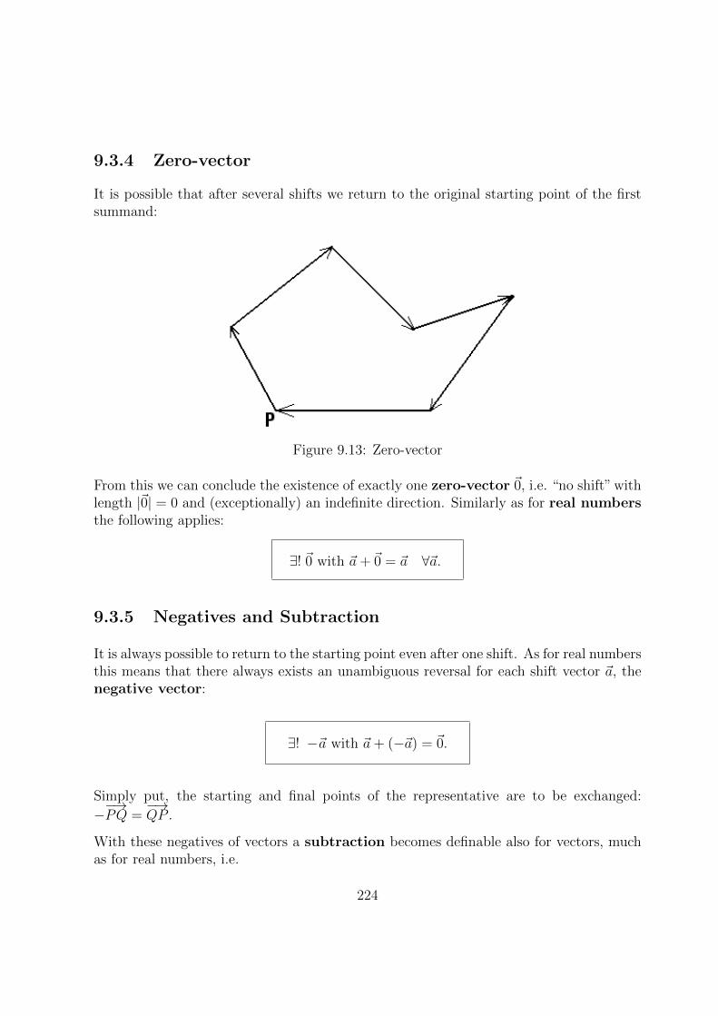
9.3.4 Zero-vector

It is possible that after several shifts we return to the original starting point of the firstsummand:

Figure 9.13: Zero-vector

From this we can conclude the existence of exactly one zero-vector ~0, i.e. “no shift” withlength |~0| = 0 and (exceptionally) an indefinite direction. Similarly as for real numbersthe following applies:

∃! ~0 with ~a+~0 = ~a ∀~a.

9.3.5 Negatives and Subtraction

It is always possible to return to the starting point even after one shift. As for real numbersthis means that there always exists an unambiguous reversal for each shift vector ~a, thenegative vector:

∃! −~a with ~a+ (−~a) = ~0.

Simply put, the starting and final points of the representative are to be exchanged:

−−→PQ =

−→QP.

With these negatives of vectors a subtraction becomes definable also for vectors, muchas for real numbers, i.e.

224

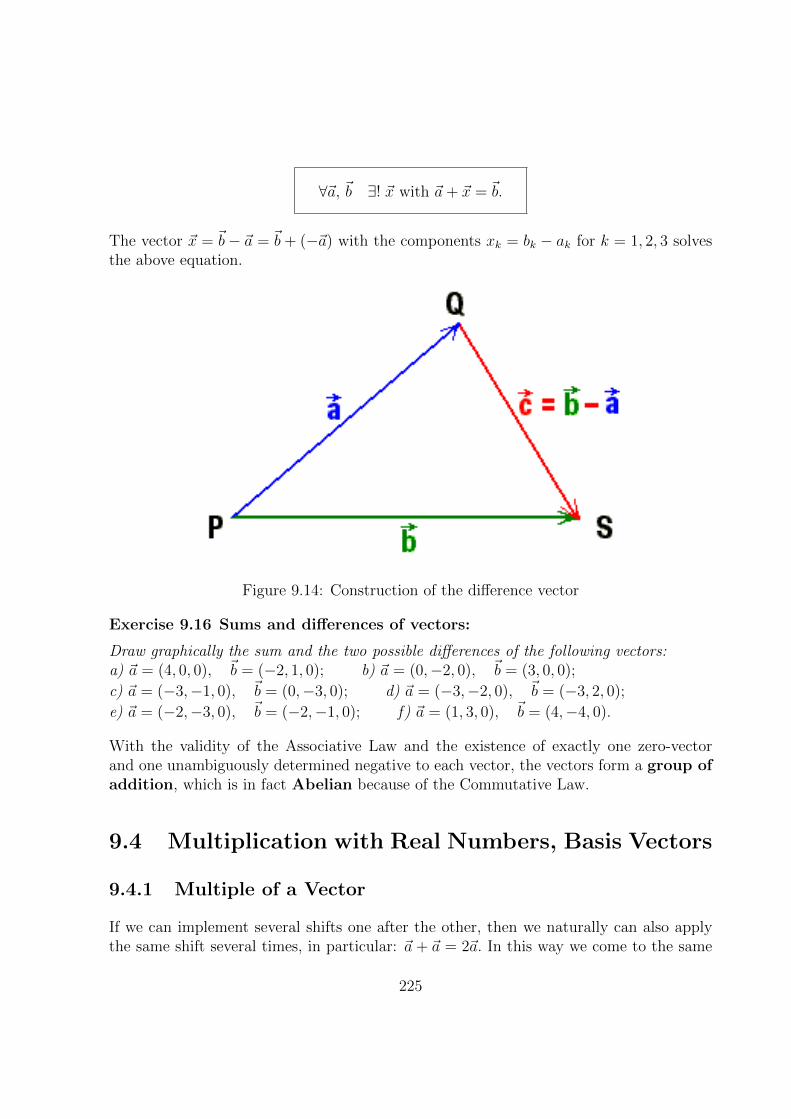
∀~a, ~b ∃! ~x with ~a+ ~x = ~b.

The vector ~x = ~b− ~a = ~b + (−~a) with the components xk = bk − ak for k = 1, 2, 3 solvesthe above equation.

Figure 9.14: Construction of the difference vector

Exercise 9.16 Sums and differences of vectors:

Draw graphically the sum and the two possible differences of the following vectors:a) ~a = (4, 0, 0), ~b = (−2, 1, 0); b) ~a = (0,−2, 0), ~b = (3, 0, 0);

c) ~a = (−3,−1, 0), ~b = (0,−3, 0); d) ~a = (−3,−2, 0), ~b = (−3, 2, 0);

e) ~a = (−2,−3, 0), ~b = (−2,−1, 0); f) ~a = (1, 3, 0), ~b = (4,−4, 0).

With the validity of the Associative Law and the existence of exactly one zero-vectorand one unambiguously determined negative to each vector, the vectors form a group ofaddition, which is in fact Abelian because of the Commutative Law.

9.4 Multiplication with Real Numbers, Basis Vectors

9.4.1 Multiple of a Vector

If we can implement several shifts one after the other, then we naturally can also applythe same shift several times, in particular: ~a + ~a = 2~a. In this way we come to the same

225

point, as we would have done if we had twice the distance in the same direction in onestep. Similarly, this holds for any real number α ∈ R as factor:

multiple: ~b = α~a with α ∈ R ⇐⇒ bk = αak for k = 1, 2, 3.

With α > 0 this yields a vector with an α-fold length into the same direction as ~a, withα < 0 the vector points in the opposite direction. As for the length we have:

|α~a| =√

(αa1)2 + (αa2)2 + (αa3)2 = |α||~a|.

9.4.2 Laws

Despite the imbalance of this product formation, the following characteristics are passeddirectly from the appropriate ones of the field of real numbers R to the present situation,because the vector components are real numbers. With the vectors ~a and ~b and the realnumbers α and β:

the Commutative Law: α~a = ~aα ⇐= αak = akα,the Associative Law: β(α~a) = (βα)~a ⇐= β(αak) = (βα)ak as well astwo Distributive Laws: (α + β)~a = α~a+ β~a ⇐= (α + β)ak = αak + βak

and α(~a+~b) = α~a+ α~b ⇐= α(ak + bk) = αak + αbk

The last law means for example graphically, that the diagonal of a parallelogram isstretched accordingly if the sides are stretched by a factor α.

9.4.3 Vector Space

If the elements of a set form an Abelian group of addition, and if multiplication with theelements of some field is defined, as was described above, mathematicians call this set avector space or simply a linear space.

Indeed, we can then form linear combinations within the space, for instance ~c = α~a+β~b,whose characteristics we want to discuss briefly in the following:

226

9.4.4 Linear Dependence, Basis Vectors

A) Firstly we consider linear combinations of two different vectors: ~a1 6= ~a2 : Two casescan occur:

A1) If an α ∈ R exists so that ~a2 = α~a1 applies, or differently expressed: if in α1~a1 +α2~a2 = 0 at least one of the factors αk 6= 0, e.g. α2 6= 0, so that the equation can besolved for ~a2, i.e. ~a2 = −α1

α2~a1 =: α~a1,

this means that the vector ~a2 can be expressed by a vector which is proportional to ~a1.The two vectors ~a1 and ~a2 are then called linearly dependent, sometimes also collinear.

A2) If there is no α such that ~a2 = α~a1 for all α ∈ R, thus ~a2 6= α~a1 or differentlyexpressed: if α1~a1 + α2~a2 = ~0 can only be achieved when both α1 = 0 and α2 = 0,

then the two vectors ~a1 =−→OA1 and ~a2 =

−→OA2 span a plane through the three points

O, A1 and A2, and each point of this plane can be represented by a linear combinationα1~a1 + α2~a2 with real factors α1 and α2.

B) Secondly we examine linear combinations of three different vectors: ~a1, ~a2 and ~a3,whereby once again two cases are possible:

B1) If two real numbers α1 and α2 can be found, such that ~a3 = α1~a1+α2~a2 or differentlyexpressed: if in α1~a1 + α2~a2 + α3~a3 = 0 at least one αk 6= 0, e.g. α3 6= 0, so that it can bedissolved for ~a3,

this means (as shown above) that ~a3 can be represented by a vector which lies completelyin the plane defined by ~a1 and ~a2. One then calls the three vectors ~a1, ~a2 and ~a3 linearlydependent, sometimes also coplanar.

B2) If ~a3 6= α1~a1 + α2~a2 or differently expressed: if α1~a1 + α2~a2 + α3~a3 = ~0 is onlyattainable when all three αk = 0 vanish,

then the three vectors ~a1, ~a2 and ~a3 span the whole space R3. We say then thatthey form a basis for R3, i.e. each three-dimensional vector is representable as a linear

combination of the three basis vectors: ∀~a =3∑

k=1

αk~ak.

C) Finally, four vectors in R3 are always linearly dependent.

Exercise 9.17 Basis vectors:

a) Do the following three vectors form a basis of R3 :(1, 3,−2), (2,−2, 1) and (4, 4,−3)?

b) What about the following three vectors:(1, 1, 0), (1,−1, 0) and (1, 1, 1)?

Particularly convenient as basis are unit vectors.

227

9.4.5 Unit Vectors

Unit vectors are dimensionless vectors of length of 1. Every unit vector specifies a directionin space. From any vector ~a we obtain the unit vector specifying to the direction bydividing by its length a, or multiplication with 1/a :

unit vector: ~ea = ~aa or ~a = a~ea.

Exercise 9.18 Unit vectors:

a) Determine the unit vector in direction of the vector ~a = (−1, 2,−2).

b) Normalize the in Lesson 9.17 assumed basis to one.

In the following we shall use the three unit vectors ~e1, ~e2 and ~e3 as basis vectors

throughout, where ~ek :=−→OEk. Sometimes the three basis vectors ~ek normalized to one

are called also a trihedral.

After we have introduced the vector components as partial shift distances along the co-ordinate axes (or equivalently as projections of the length of the vector on the coordinateaxes) it follows directly:

~a = a1~e1 + a2~e2 + a3~e3 =3∑

k=1

ak~ek (≡ ak~ek with Einstein summation convention!).

Since we selected not just any skew, but a Cartesian coordinate system at the beginning

of this chapter, we know that the three unit vectors ~ek :=−−→OEk are pairwise perpendicular

one another, and thus form an orthonormal (i.e. orthogonal and normalized) basis(ONB). In order to be able to express this fact in formulae, we need a quantity connectedwith the angle between two vectors, which says for instance that with a right angle betweenthem the projection of one vector onto the other disappears. This task leads us to thequestion of multiplication of two vectors which we will treat in the next section.

Insert: Active Viewpoint: In our considerations concerning transformationswe have always been asking only the question of, how the components of a fixed vectorwould look like, if we had changed the describing coordinate system or rather the basisvectors. Then the same vector ~a will be represented with respect to the two differentorthonormal bases ~ek rather ~ke by different components ak and ak, respectively:

~a = ak~ek = ak~ke. If in this case ~ke = D(3)kl (ϕ)~el for instance would be rotated around

228

the 3-axis by an angle ϕ clockwise looking in positive 3-direction, the components

ak = D(3)kl (ϕ)al would rotate correspondingly, as we have seen. This situation is

called the passive viewpoint and we will take this viewpoint consequently duringthe whole course. This problem is of great importance because physicists have tomake sure that their laws are formulated in such a manner that they are independentof the chosen coordinate system.

Physicists have, however, in addition another, at first sight fully different prob-lem, namely the mathematical description of mass points, vectors, etc. which reallymove in space (e.g. with time) for instance rotate. In this case we have to describethe original vector ~a and the physical vector ~a, which was e.g. rotated around the3-axis by an angle φ clockwise looking in positive 3-direction, in one and the samecoordinate system ~ek: ~a = ak~ek and ~a = ak~ek. This situation is called the active

viewpoint. The following figure shows you that in this case holds ak = D(3)kl (−ϕ)al.

Figure 9.15: Difference between passive and active viewpoint

In both cases we have intentionally used the hat to label the new components tosignalize clearly that the relation

ak = D(3)kl (ϕ)al

may have two fully different meanings, namely:

1. the transformed components of a vector ~a as linear combination of the oldones in case of a rotation of the coordinate system by an angle ϕ around the3-direction and

2. the components of a vector after its rotation by an angle −ϕ around the 3-direction as linear combination of its components before the rotation.

If you have clarified both situations only once, there is scarcely any danger of con-

fusion, but rather pleasure about the fact that you are able to solve two problems at

once by studying the same rotation matrices.

229

9.5 Scalar Product and the Kronecker Symbol

9.5.1 Motivation

In order to describe the orthogonality of our basis vectors, and also for physical reasons,we need a product of two vectors which measures the angle between the two factorsand is connected with the projection of one vector onto the other. For constrainedmotions (for instance along rails or on an inclined plane) not the entire applied force, butonly its projection (onto the rails or onto the plane) is the crucial physical quantity. Alsofor the computation of the work which must be done in order to displace a mass againsta force (e.g. the force of gravity) not the entire force, but only its projection onto thedisplacement direction is the really determining quantity.

Exercise 9.19 Work:

How can we calculate the work which must be done,a) if the mass m of a mathematical pendulum with thread length r is to be deflected by anangle ϕ?b) if a mass point m is to be pushed up a distance ϕ along an inclined plane, with incli-nation angle s relative to the horizontal plane?

9.5.2 Definition

Thus we choose the following definition for a “product” between two vectors ~a and ~b andcall it the “scalar product”, because it gives us for every two factor vectors a real number,and as we later show that this number transforms as a scalar. Because of the dot betweenthe two factors often used in English literature, the alternative name “dot product” is alsocommon.

scalar product (~a ·~b) := |~a| · |~b| cos∠(~a,~b) = ab cosϕ.

Besides the two trivial factors of the lengths of the two vectors, we select the cosine ofthe angle ϕ = ∠(~a,~b) included by both the representatives with the same starting point,because this cosine vanishes if ϕ = 90 i.e. if the two vectors stand perpendicular one tothe other. Clearly the expression b cosϕ is the projection of the vector ~b on the directionof ~a and a cosϕ the projection of the vector ~a on the direction of ~b. These projections aremultiplied in each case by the length of the vector on whose direction was projected, andare provided with a minus sign when the angle is obtuse. Thus the numerical value of the

230

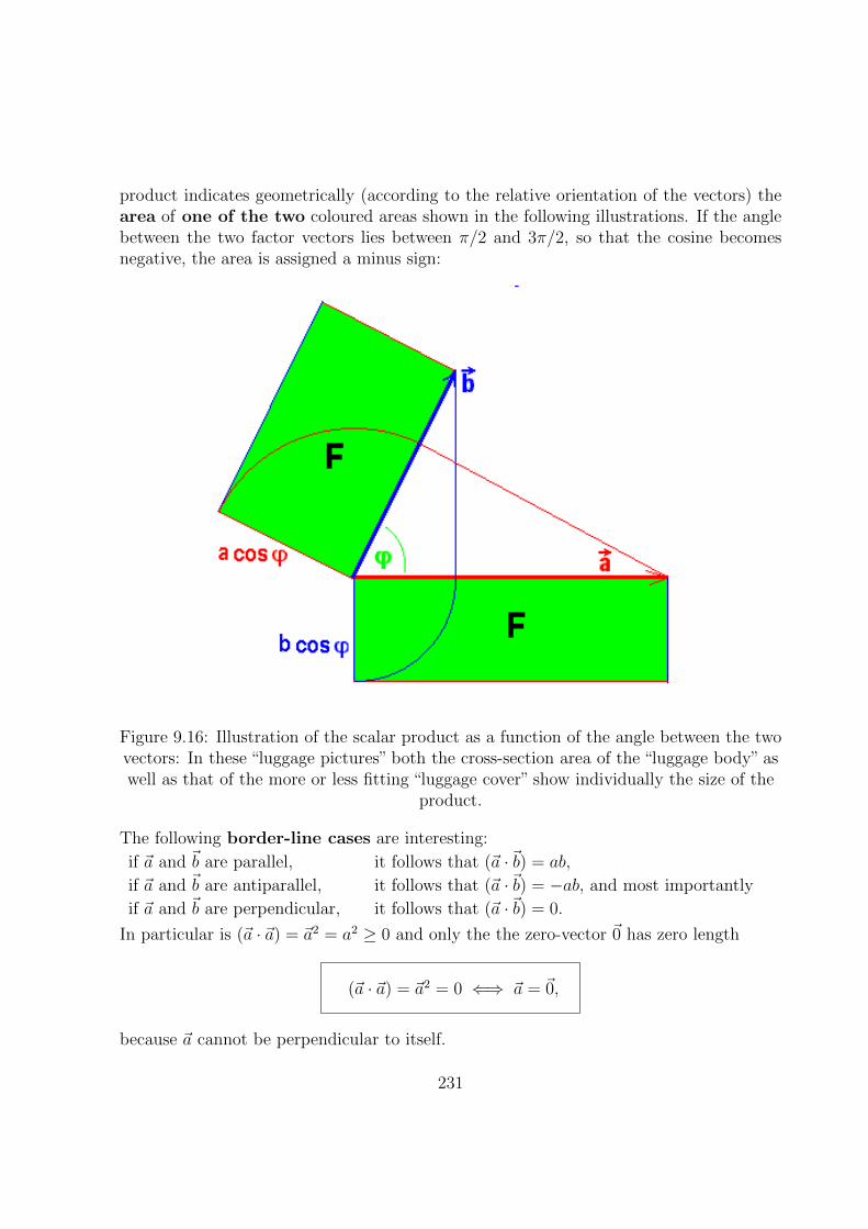
product indicates geometrically (according to the relative orientation of the vectors) thearea of one of the two coloured areas shown in the following illustrations. If the anglebetween the two factor vectors lies between π/2 and 3π/2, so that the cosine becomesnegative, the area is assigned a minus sign:

Figure 9.16: Illustration of the scalar product as a function of the angle between the twovectors: In these “luggage pictures” both the cross-section area of the “luggage body” aswell as that of the more or less fitting “luggage cover” show individually the size of the

product.

The following border-line cases are interesting:

if ~a and ~b are parallel, it follows that (~a ·~b) = ab,

if ~a and ~b are antiparallel, it follows that (~a ·~b) = −ab, and most importantly

if ~a and ~b are perpendicular, it follows that (~a ·~b) = 0.

In particular is (~a · ~a) = ~a2 = a2 ≥ 0 and only the the zero-vector ~0 has zero length

(~a · ~a) = ~a2 = 0 ⇐⇒ ~a = ~0,

because ~a cannot be perpendicular to itself.

231

Exercise 9.20 Angle in the scalar product

What does 2(~a ·~b) = |~a| · |~b| mean for the angle between the two vectors?

Exercise 9.21 Cosine Theorem

a) Prove with the help of the scalar product the Cosine Theorem of plane geometry, ac-cording to which in a triangle with the side lengths a, b and c: c2 = a2 + b2 − 2ab cos γapplies, where γ is the angle opposite to side c.

b) What follows from this theorem for γ = π/2?

Exercise 9.22 Schwarz inequality

Why does the Schwarz inequality hold for the absolute value of the scalar product: |(~a·~b)| ≤|~a| · |~b| ?

9.5.3 Commutative Law

The previous definition of the scalar product treats the two factors in a completely sym-metric way. Therefore trivially the

Commutative Law: (~a ·~b) = (~b · ~a).

applies.

9.5.4 No Associative Law

The scalar product consisting of two absolute values and a cosine is obviously not a vector,but rather a real number. (Because of the symmetry we refrained from adding one of thetwo vectors. Thus our product is not an “internal linkage” in vector space. For thisreason we prefer to avoid the sometimes used designation “inner product” used sometimes.Since the result of the multiplication is not a vector, we obviously cannot multiply it ina scalar product with a third vector. Thus, there is no Associative Law for the scalarproduct. For the same reason we cannot expect that vectors form a group of multiplicationunder this product.

Exercise 9.23 On the Associative Law

a) Compare the vector (~a ·~b)~c with the vector ~a(~b · ~c) geometrically.

b) What is the meaning of ~a3 ?

232

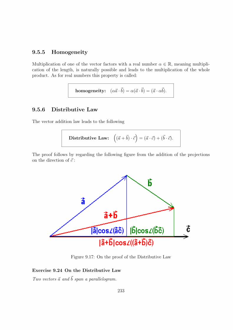
9.5.5 Homogeneity

Multiplication of one of the vector factors with a real number α ∈ R, meaning multipli-cation of the length, is naturally possible and leads to the multiplication of the wholeproduct. As for real numbers this property is called:

homogeneity: (α~a ·~b) = α(~a ·~b) = (~a · α~b).

9.5.6 Distributive Law

The vector addition law leads to the following

Distributive Law:(

(~a+~b) · ~c)

= (~a · ~c) + (~b · ~c).

The proof follows by regarding the following figure from the addition of the projectionson the direction of ~c :

Figure 9.17: On the proof of the Distributive Law

Exercise 9.24 On the Distributive Law

Two vectors ~a and ~b span a parallelogram.

233

a) Calculate in addition the following scalar product(

(~a+~b) · (~a−~b)).

b) What is the geometrical meaning of this scalar product?

c) Determine the angle ϕ between the two diagonals of the parallelogram.

d) When are these perpendicular to each other?

9.5.7 Basis Vectors

In the definition of the scalar product, among other things we were motivated by the wishto be able to describe the orthogonality of the three normalized basis vectors ~ek ofthe Cartesian coordinate system in a simple way. As desired we now get three equations:

orthogonality: (~ek · ~el) = |~ek||~el| cos∠(~ek, ~el) = cosϕkl = 0 for k 6= l = 1, 2, 3,

because ϕkl = π/2 or equivalently ~ek ⊥ ~el for k 6= l. For k = l we obtain three furtherequations:

normalization: (~ek · ~ek) = |~ek||~ek| cos∠(~ek, ~ek) = cos 0 = 1 for k = 1, 2, 3.

9.5.8 Kronecker Symbol

Those nine equations contain all information about the orthogonality and normalizationof the basis vectors. They can be combined into one single equation

orthonormality: (~ek · ~el) = δk l,

if we introduce the symbol δk l named after Leopold Kronecker, which is defined as follows:

Kronecker symbol: δk l :=

1 for k = l0 for k 6= l.

Like the scalar product, this number pattern is symmetrical against exchange of the twoindices: δk l = δl k. In the following figure the pattern is pictorially represented in a plane:

234

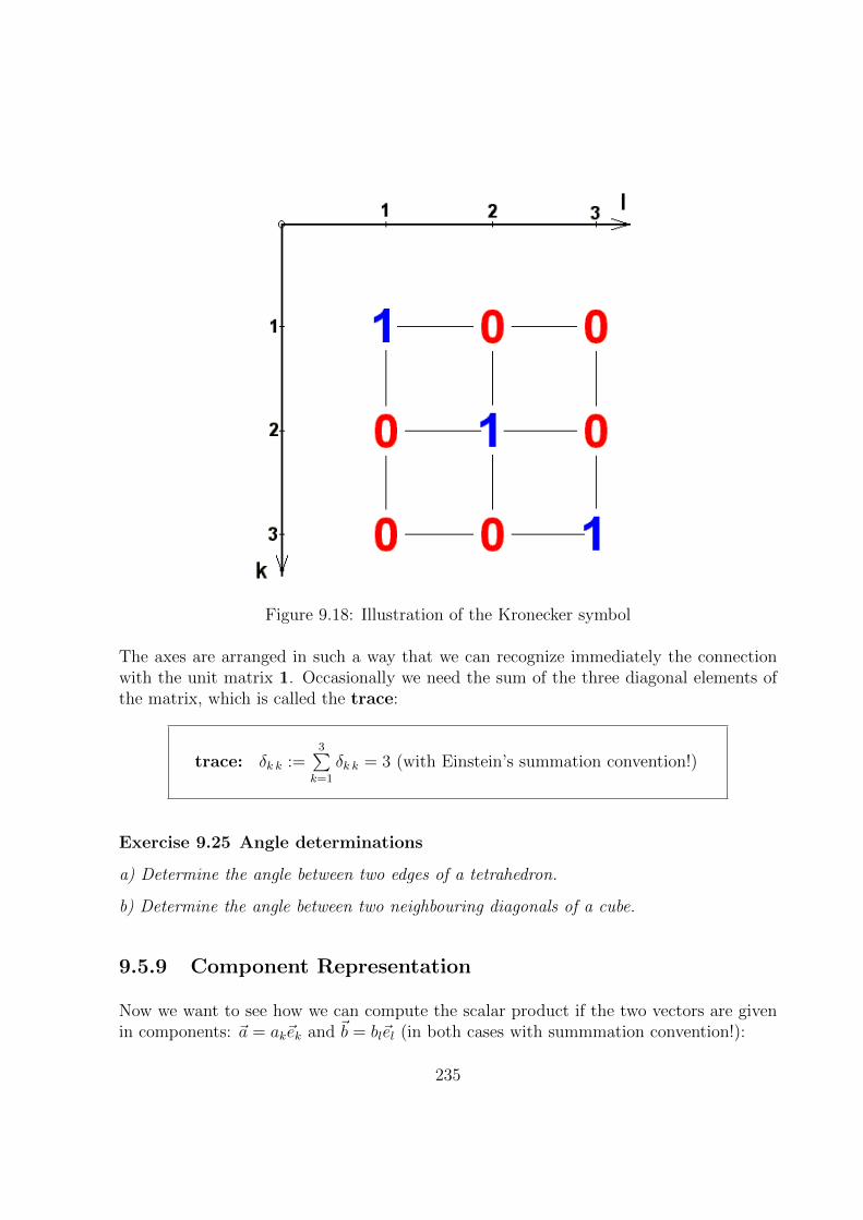
Figure 9.18: Illustration of the Kronecker symbol

The axes are arranged in such a way that we can recognize immediately the connectionwith the unit matrix 1. Occasionally we need the sum of the three diagonal elements ofthe matrix, which is called the trace:

trace: δk k :=3∑

k=1

δk k = 3 (with Einstein’s summation convention!)

Exercise 9.25 Angle determinations

a) Determine the angle between two edges of a tetrahedron.

b) Determine the angle between two neighbouring diagonals of a cube.

9.5.9 Component Representation

Now we want to see how we can compute the scalar product if the two vectors are givenin components: ~a = ak~ek and ~b = bl~el (in both cases with summmation convention!):

235

(~a ·~b) = (ak~ek · bl~el) whereby both over k and l are summed up= akbl(~ek · ~el) because of the homogeneity of the scalar product= akblδk l because of the orthonormality of the basis vectors= akbk because of the Kronecker symbol only the term

l = k of the sum over l remains. Therefore only the sum overk = 1, 2, 3 remains, thus

component representation: (~a ·~b) = a1b1 + a2b2 + a3b3 = akbk

Exercise 9.26 Kronecker symbol

Prove the above formula in detail by explicit multiplication of the brackets((a1~e1 + a2~e2 + a3~e3) · (b1~e1 + b2~e2 + b3~e3)) without use of the Kronecker symbol, so thatyou can estimate, how much calculation work you save using the symbol.

Exercise 9.27 Orthonormal basis

Do the three vectors, ~a1 = 1√2(1, 1, 0), ~a2 = 1√

2(1,−1, 2) and ~a3 = 1√

3(1,−1,−1) form an

orthonormal basis of the vector space?

Especially for one of the three basis vectors we find:

(~ek · ~a) = (~ek · al~el) = al(~ek · ~el) = alδk l = ak,

in detail with sum signs: (~ek · ~a) =3∑l=1

(~ek · al~el) =3∑l=1

al(~ek · ~el) =3∑l=1

alδk l = ak, the k-

component of the vector ~a, because the scalar multiplication with the basis vector numberk results in the projection of the vector on the k-axis. From this we can easily reconstructthe entire vector ~a:

~a = ~ekak = ~ek(~ek · ~a).

Insert: Completeness: If we place two superfluous brackets “)” in the equation~a = ~ekak = ~ek (~ek · ~a), we get:

~a) = ~ek) (~ek · ~a)

or from this the abstract, famous symbolic

completeness relation: ~ek) (~ek = 1.

236

After scalar multiplication from the left or right with a vector we obtain from thecompleteness relation the component representation of the vector ~a = ~ekak : forinstance from the right: ~ek) (~ek ·~a) = ~ekak= 1 ~a) = ~a or from the left: (~a ·~ek) (~ek =ak~ek = (~a 1 = ~a.

In particular for the basis vectors themselves:

~el = ~ekδk l

from ~el = ~el) = 1 ~el) = ~ek) (~ek · ~el) = ~ekδk l.

This means that the columns or lines of the Kronecker symbol are simply the com-

ponents of the basis vectors.

Exercise 9.28 Scalar product

Determine the scalar product and the lengths of the projections for the two vectors ~a =(4,−2, 4) and ~b = (−2, 3, 6).

Exercise 9.29 Angle with the coordinate axes

Which angles does the vector ~a = ~e1 +√

3~e2 form with the coordinate axes?

9.5.10 Transverse Part

Apart from the decomposition in terms of components with respect to a selected coordi-nate system, a further decomposition of a vector ~a (e. g. of an oscillation vector) is neededfrequently in physics, namely in a “longitudinal part” a‖e with respect to an arbitrarilygiven direction ~e (e.g. the direction of the propagation of a wave) and the “transversepart” ~a⊥e with (~a⊥e · ~e) = 0. From the decomposition ansatz ~a = a‖e~e + ~a⊥e we get bymultiplication with ~e : (~a · ~e) = a‖e and from this by insertion ~a = (~a · ~e)~e+~a⊥e and fromthis by insertion

transverse part: ~a⊥e = ~a− (~a · ~e)~e

Exercise 9.30 Transverse part:

Calculate for the vector ~b = (1, 2,−2) the part which is transverse to ~a = (3, 6, 3).

237

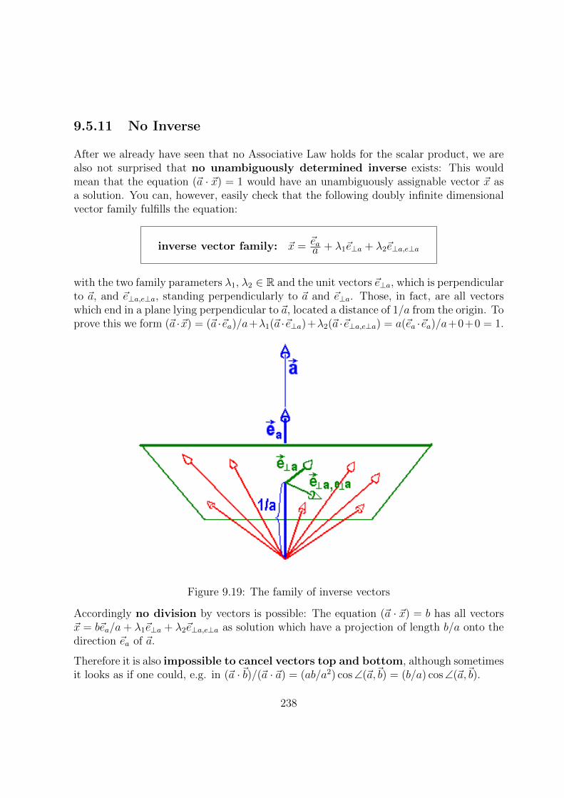
9.5.11 No Inverse

After we already have seen that no Associative Law holds for the scalar product, we arealso not surprised that no unambiguously determined inverse exists: This wouldmean that the equation (~a · ~x) = 1 would have an unambiguously assignable vector ~x asa solution. You can, however, easily check that the following doubly infinite dimensionalvector family fulfills the equation:

inverse vector family: ~x = ~eaa + λ1~e⊥a + λ2~e⊥a,e⊥a

with the two family parameters λ1, λ2 ∈ R and the unit vectors ~e⊥a, which is perpendicularto ~a, and ~e⊥a,e⊥a, standing perpendicularly to ~a and ~e⊥a. Those, in fact, are all vectorswhich end in a plane lying perpendicular to ~a, located a distance of 1/a from the origin. Toprove this we form (~a ·~x) = (~a ·~ea)/a+λ1(~a ·~e⊥a)+λ2(~a ·~e⊥a,e⊥a) = a(~ea ·~ea)/a+0+0 = 1.

Figure 9.19: The family of inverse vectors

Accordingly no division by vectors is possible: The equation (~a · ~x) = b has all vectors~x = b~ea/a+ λ1~e⊥a + λ2~e⊥a,e⊥a as solution which have a projection of length b/a onto thedirection ~ea of ~a.

Therefore it is also impossible to cancel vectors top and bottom, although sometimesit looks as if one could, e.g. in (~a ·~b)/(~a · ~a) = (ab/a2) cos∠(~a,~b) = (b/a) cos∠(~a,~b).

238

Exercise 9.31 Inverse vector family:

Find explicitly a family of vectors ~x which solves the equation (~a · ~x) = 1, if ~a = (1, 2, 2).

9.6 Vector Product and the Levi-Civita Symbol

9.6.1 Motivation

We now have a commutative product of two vectors. Granted, it is only a scalar onelacking associative law and a unique inverse. But it does provide a simple and compactcharacterization of the orthonormality of our basis vectors and, above all, a reasonableand appropriate description of all the many physical situations in which the projection ofone vector onto another plays an important role.

However, we cannot settle for just this. First of all we want to at least try to find agenuine vector product which assigns to two vectors again an element of the vector space.Secondly we want a nice simple expression of the fact that our basis vectors form a right-handed coordinate system. Finally we know a whole crowd of vector-like quantities inphysics which cannot be brought so simply in connection with displacements for instanceangular momentum and torque - but have very much to do with rotations of extendedrigid bodies around an axis. The existence of a vector product the scalar product is, bythe way, a special characteristic of the three-dimensional space; for vectors in R2 and R4

such a product does not exist.

Figure 9.20: Rotating motion

As we see from the figure, no cosine determines any thing. The interacting quantityis F sinϕ, the projection of the force perpendicular to the line connecting the axis of

239

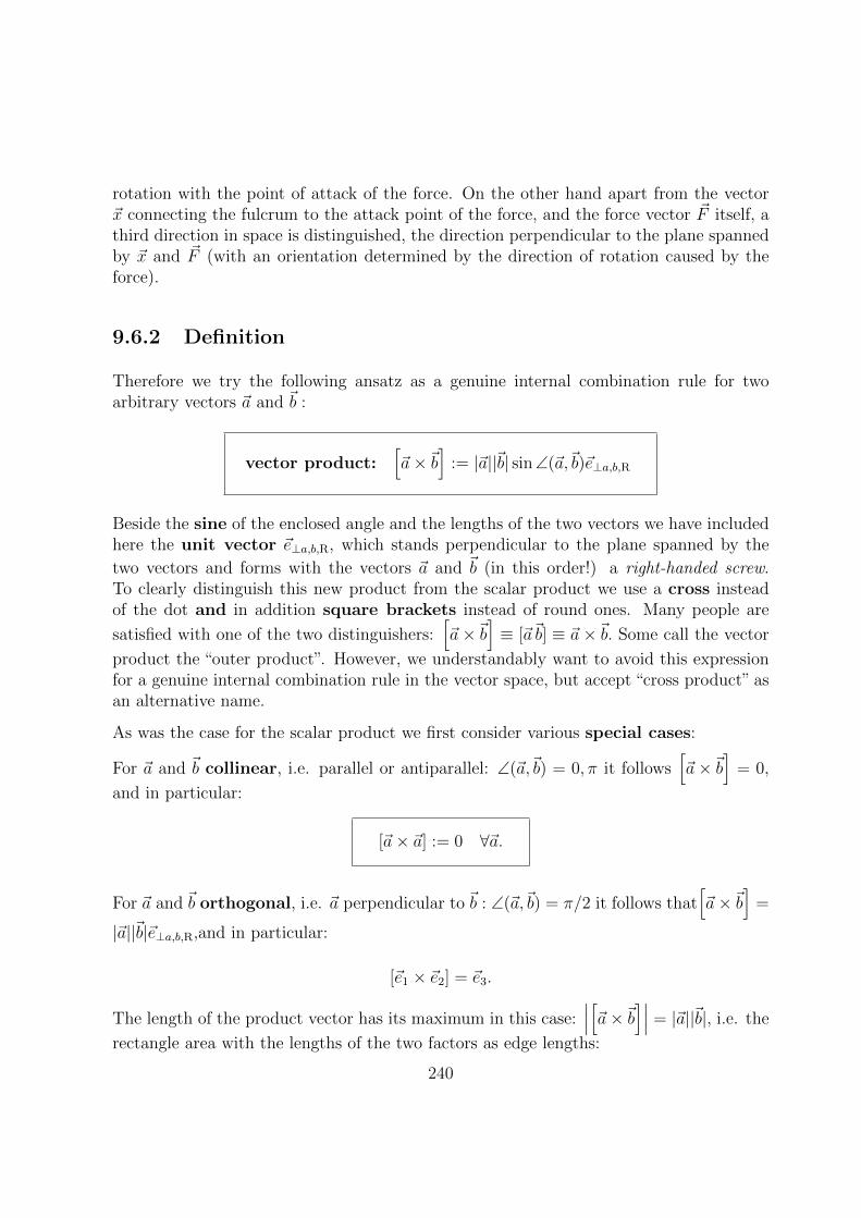
rotation with the point of attack of the force. On the other hand apart from the vector~x connecting the fulcrum to the attack point of the force, and the force vector ~F itself, athird direction in space is distinguished, the direction perpendicular to the plane spannedby ~x and ~F (with an orientation determined by the direction of rotation caused by theforce).

9.6.2 Definition

Therefore we try the following ansatz as a genuine internal combination rule for twoarbitrary vectors ~a and ~b :

vector product:[~a×~b

]:= |~a||~b| sin∠(~a,~b)~e⊥a,b,R

Beside the sine of the enclosed angle and the lengths of the two vectors we have includedhere the unit vector ~e⊥a,b,R, which stands perpendicular to the plane spanned by the

two vectors and forms with the vectors ~a and ~b (in this order!) a right-handed screw.To clearly distinguish this new product from the scalar product we use a cross insteadof the dot and in addition square brackets instead of round ones. Many people are

satisfied with one of the two distinguishers:[~a×~b

]≡ [~a~b] ≡ ~a×~b. Some call the vector

product the “outer product”. However, we understandably want to avoid this expressionfor a genuine internal combination rule in the vector space, but accept “cross product” asan alternative name.

As was the case for the scalar product we first consider various special cases:

For ~a and ~b collinear, i.e. parallel or antiparallel: ∠(~a,~b) = 0, π it follows[~a×~b

]= 0,

and in particular:

[~a× ~a] := 0 ∀~a.

For ~a and ~b orthogonal, i.e. ~a perpendicular to ~b : ∠(~a,~b) = π/2 it follows that[~a×~b

]=

|~a||~b|~e⊥a,b,R,and in particular:

[~e1 × ~e2] = ~e3.

The length of the product vector has its maximum in this case:∣∣∣[~a×~b]∣∣∣ = |~a||~b|, i.e. the

rectangle area with the lengths of the two factors as edge lengths:

240

Figure 9.21: The rectangle∣∣∣[~a×~b]∣∣∣ = |~a||~b|

In the general case the length of the product vector is∣∣∣[~a×~b]∣∣∣ = |~a||~b| sin∠(~a,~b),

the area of the parallelogram spanned by both factors or equally one of the two rectangleareas associated with the heights of the parallelogram, shown coloured in the next picture.

Figure 9.22: Illustration of the length of the vector product as a function of the anglebetween the two vectors: The areas of the parallelogram and also of each of the two

rectangles with the heights of the parallelogram show the length of the vector product.

241

If the angle between the factor vectors exceeds π, the sine and therefore also the areabecomes negative, which leads here to a reversal of the direction of the product vector.

Exercise 9.32 Physical vector products

How do you obtain:

a) the linear velocity ~v during a rotating motion from the angular velocity ~ω = ~eωdϕ/dtand the position vector ~x?

b) the “area velocity” ~f in the Kepler motion from the position vector ~x and the velocity~v of the planet?

c) the angular momentum ~L from the position vector ~x and the momentum ~p?

d) the mechanical torque ~D from the force ~F and the moment arm ~x?

e) the torque on an electrical dipole with dipole moment ~p in a homogeneous electrical field~E?

f) the torque on a magnetic dipole with dipole moment ~m in a homogeneous magnetic field~H?

g) the density of the electromagnetic Lorentz force ~k from the velocity ~v of an electron

with mass m and charge e and the magnetic induction ~B ?

h) the Poynting vector ~S of the electromagnetic radiant flux from the electric field ~E and

magnetic field ~H of the radiation?

i) the magnetic field ~H in the distance ~x from a linear electric current density ~j accordingto the Biot-Savart law?

Exercise 9.33 Torques

Discuss the amount and the direction of the torque on a compass needle in the magneticfield of the earth, if the angle ϑ = ∠(~m, ~H) between the dipole moment ~m and the field~H : is 0, π/4, π/2, 3π/4, π, 5π/4.

242

Exercise 9.34 Balance of the torques

Figure 9.23: What force ~F4 must act at the indicated place so that the rigid T-fittinghere does n o t turn around the fulcrum 0?

9.6.3 Anticommutative

The direction of the product vector obviously depends on the order of the factors asexpressed by the right screw rule, which is determined by the physical interpretation of

the rotation, e.g. as in the case of torque: ~D =[~x× ~F

]. Thus no Commutative Law

holds, but the cross product is:

anticommutative:[~b× ~a

]= −

[~a×~b

]

In particular we have: [~e2 × ~e1] = −~e3 for the basis vectors.

9.6.4 Homogeneity

Just as for the scalar product, however:

243

homogeneity: [α~a×~b] = α[~a×~b

]= [~a× α~b]

applies to the vector product in both factors for multiplication by a real number α ∈ R.

9.6.5 Distributive Law

As expected there also holds a

Distributive Law: [(~a1 + ~a2)×~b] =[~a1 ×~b

]+[~a2 ×~b

].

However, its proof is not trivial, since the transversal parts of the vectors are needed.

Insert: Distributive Law: We call the sum ~a1 +~a2 =: ~a3, the unit vector inthe direction of ~b : ~eb := ~b/b and consider the transverse parts of the two summandswith respect to the direction of ~b ~a

k⊥~b = ~ak− (~ak~eb)~eb for k = 1, 2 and also for k = 3because of the Distributive Law for the scalar product. These transverse parts all liein the plane perpendicular to ~eb as shown in the next figure:

Figure 9.24: The plane perpendicular to ~b.

244

The product vectors [~ak⊥b × ~eb] are then vectors of length ak⊥b which, rotated by 90

counterclockwise, are perpendicular to ~ak⊥b. This means, however, that the whole

vector addition figure was rotated by 90, so that [ ~a3⊥b × ~eb] = [ ~a1⊥b × ~eb] +

[ ~a2⊥b × ~eb] holds. Multiplication of this equation with b yields the desired Distributive

Law.

Exercise 9.35 Distributive law for vector products

a) Calculate: [(~a+~b)× (~a−~b)].

b) How reads the Lagrange-identity:[~a×~b

]2

+ (~a ·~b)2 =?

c) What is therefore the meaning of

√[~a×~b

]2

+ (~a ·~b)2 = b2 for the vector ~a?

d) Calculate the sum of the outer normals of a tetrahedron.

9.6.6 With Transverse Parts

We can use the concept of the transverse part of a vector with respect to a given direction,which we defined and studied earlier, in order to shed new light on the illustrativemeaning of the vector product: To do this, we take the transverse part of the secondfactor ~b with respect to the direction ~ea = ~a/a of the first factor: ~b⊥a = ~b−(~b ·~ea)~eaand multiply ~a vectorially by this:

[~a×~b⊥a

]=[~a×~b

]− (~b · ~ea) [~a× ~ea] =

[~a×~b

].

Since a corresponding argument can also be given for the other factor, this means: In thevector product one factor can be replaced by its transverse part with respectto the other one without changing the value of the product.

For a better understanding look once more at Figure 9.22.

9.6.7 Basis Vectors

In order to obtain a component representation for our vector product, the basis vectorsfirst must be multiplied vectorially. As already suggested above, the vector product givesus the desired simple representation of the fact that our basis vectors form a right-handedsystem:

245

right-handed system: [~e1 × ~e2] = ~e3, [~e2 × ~e3] = ~e1, [~e3 × ~e1] = ~e2.

Because of the anticommutativity of the vector product three further relations with thereverse order of the factors and a minus sign can be added:

[~e2 × ~e1] = −~e3, [~e3 × ~e2] = −~e1, [~e1 × ~e3] = −~e2.

Much as for the scalar product and the Kronecker symbol we summarize these six fun-damental relations into one single equation by the introduction of the symbol designatedafter Tullio Levi-Civita:

9.6.8 Levi-Civita Symbol

We simply write:

right-handed coordinate system: [~ek × ~el] = εklm~em ≡∑3

m=1 εklm~em

where the last term once more reminds us of the Einstein summation convention. Herethe Levi-Civita symbol with its three indices is defined by:

Levi-Civita symbol: εklm :=

+1, if klm = 123, 231, 312,−1, if klm = 132, 213, 321 and0 otherwise

Obviously the symbol changes sign when permuting any two indices. One calls the symboltotally antisymmetric against exchanging pairs of indices:

total antisymmetry: εklm = εlmk = εmkl = −εkml = −εlkm = −εmlk

For all even or cyclic permutations of the sequence of index numbers 123 a +1 results,yielding exactly the three relations indicated above, characteristic of a right-handed basis.The index sequences with an odd number of permutations of two indices against the num-ber sequence 123 or anticyclic permutations of 123 lead to −1, as in the three previouslyspecified vector products with exchanged order of the factors. Only six of the 27 elementsof the Levi-Civita symbol are different from 0. All 21 remaining elements are zeros,so that you may have trouble finding the important three blue “ones” in the crowd ofred zeros, arranged remarkably symmetrically from the origin in the following figure, andespecially the even more important three −1 in green:

246

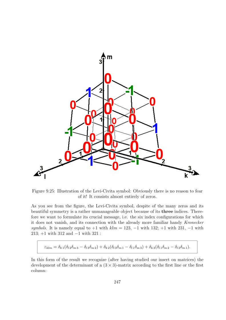
Figure 9.25: Illustration of the Levi-Civita symbol: Obviously there is no reason to fearof it! It consists almost entirely of zeros.

As you see from the figure, the Levi-Civita symbol, despite of the many zeros and itsbeautiful symmetry is a rather unmanageable object because of its three indices. There-fore we want to formulate its crucial message, i.e. the six index configurations for whichit does not vanish, and its connection with the already more familiar handy Kroneckersymbols. It is namely equal to +1 with klm = 123, −1 with 132; +1 with 231, −1 with213; +1 with 312 and −1 with 321 :

εklm = δk 1(δl 2δm 3 − δl 3δm 2) + δk 2(δl 3δm 1 − δl 1δm 3) + δk 3(δl 1δm 2 − δl 2δm 1).

In this form of the result we recognize (after having studied our insert on matrices) thedevelopment of the determinant of a (3× 3)-matrix according to the first line or the firstcolumn:

247

εklm = +δk 1

∣∣∣∣∣∣δl 2 δl 3

δm 2 δm 3

∣∣∣∣∣∣+ δk 2

∣∣∣∣∣∣δl 3 δl 1

δm 3 δm 1

∣∣∣∣∣∣+ δk 3

∣∣∣∣∣∣δl 1 δl 2

δm 1 δm 2

∣∣∣∣∣∣ .Thus:

εklm =

∣∣∣∣∣∣δk 1 δk 2 δk 3

δl 1 δl 2 δl 3δm 1 δm 2 δm 3

∣∣∣∣∣∣ =

∣∣∣∣∣∣δk 1 δl 1 δm 1

δk 2 δl 2 δm 2

δk 3 δl 3 δm 3

∣∣∣∣∣∣ =

∣∣∣∣∣∣δ1 k δ1 l δ1m

δ2 k δ2 l δ2m

δ3 k δ3 l δ3m

∣∣∣∣∣∣ = . . .

In the transition from the first to the second version we used that the determinant of amatrix A is not changed by reflection through the main diagonal: |AT | = |A|. In thetransition to the third version we used the symmetry of the Kronecker symbol against ex-changing the two indices: δk 1 = δ1 k. There is obviously still an abundance of further formsof the Levi-Civita symbol as determinant, if we consider that each determinant changesits sign when exchanging two lines or columns. Using the determinant representation ofthe Levi-Civita symbol you should always remember that the Kronecker symbols in thedeterminant are nothing other than place holders, which tell you depending on the valueof the indices whether there is a 1 or a 0 in this place.

Exercise 9.36 Normal vectors

Which unit vectors are perpendicular to:

a) (~e1 + ~e2) and (~e1 − ~e2),

b) (~e1 − ~e2) and (~e2 − ~e3),

c) (~e1 + 2~e3) and (~e2 − 2~e3)?

Exercise 9.37 Tetrahedron surface

Calculate by means of vector products, the surface of a tetrahedron of edge length L byembedding it into a cube of the edge length a.

9.6.9 Component Representation

Now we are able to calculate the vector product of two vectors ~a = ak~ek and ~b = bl~el fromtheir components:

248

component representation:[~a×~b

]= [ak~ek × bl~el] = akbl [~ek × ~el] = εklmakbl~em

We would like to remind you once more of the fact that the right side of this equationcontains - according to the Einstein convention - three sums over k = 1, 2, 3, l = 1, 2, 3and m = 1, 2, 3. Thus there are altogether 27 summands, of which 21 we do not needto be afraid of, because we know that they vanish. Only the following six terms remainnon-zero, three of them with the characteristic minus signs:

[~a×~b

]= ~e1(a2b3 − a3b2) + ~e2(a3b1 − a1b3) + ~e3(a1b2 − a2b1)

Here the six summands are organized according to basis vectors, to be able to recognizemore easily that e.g.: the 1-component of the product vector is constructed from com-

ponents of the two factors as follows:[~a×~b

]1

= (a2b3 − a3b2). Generally for the m-th

component we get:

[~a×~b

]m

= ([~a×~b

]· ~em) = εklmakbl(~em · ~em) = εklmakbl = εmklakbl.

The final way of writing is justified because of the cyclic permutability of the indices inthe Levi-Civita symbol.

Our representation of the Levi-Civita symbol as a determinant of Kronecker symbolspermits even more ways of writing down the component representation of the vectorproduct. These can easily be kept in mind and may be known to some of you :

[~a×~b

]= akbl~em

∣∣∣∣∣∣δk 1 δk 2 δk 3


∣∣∣∣∣∣ =

∣∣∣∣∣∣a1 a2 a3

b1 b2 b3

~e1 ~e2 ~e3

∣∣∣∣∣∣ =

∣∣∣∣∣∣~e1 ~e2 ~e3

a1 a2 a3

b1 b2 b3

∣∣∣∣∣∣ = . . .

In order to obtain the final form in the preceding determinant, the lines were cyclicallypermuted. In this manner or e.g. by reflection of the determinant in its main diagonal,you can find again a whole set of representations which are all equivalent, since they leadto the same result. In practice you will naturally pay attention to existing zeros and selectthat form, from which you can see the desired result immediately.

249

In the last two forms the determinant way of writing is clearly meant symbolically and tobe enjoyed with some caution, because, as you see, the basis vectors stand as elements inthe determinant, and an object of this kind has actually not been defined. The meaningof this determinant is an easily remembered expression for the following frequently useddevelopment with respect to the adjuncts:

[~a×~b

]= ~e1

∣∣∣∣∣∣a2 a3

b2 b3

∣∣∣∣∣∣− ~e2

∣∣∣∣∣∣a3 a1

b2 b1

∣∣∣∣∣∣+ ~e3

∣∣∣∣∣∣a1 a2

b1 b2

∣∣∣∣∣∣

Exercise 9.38 Vector product as determinant

Calculate the vector products of Exercise 9.36 as determinants.

9.6.10 No Inverse

With this component decomposition we have defined in convenient form for our physicaluse a genuine vector product of two vectors. However, again some characteristics aremissing, which would be essential for the formation of a group: As is the case for thescalar product there is no unambiguously determined inverse ~x which solves the equation[~a× ~x] = ~e, but again a whole family of vectors

inverse vector family: ~x(λ) =~e⊥a,ea + λ~a.

This inverse vector family includes all vectors with representatives which have their tipson a straight line parallel to ~a a distance of 1/a from the origin. Moreover, no divisionexists, because the vector family ~x(λ) = (b/a)~e⊥a,b + λ~a with the family parameter λ ∈ R(perhaps with a dimension) solves the equation [~a× ~x] = ~b. In order to see this, we go to

a plane perpendicular to ~b in the next figure:

250

Figure 9.26: Concerning division by a vector

In this plane we draw (in the foot point of the selected representative of ~a perpendicularto this) the vector (b/a)~e⊥a,b and add to its tip the vector λ~a parallel to ~a to obtain thedesired vector family ~x(λ). The lengths of all product vectors [~a× ~x] are the areas of theparallelograms spanned by ~a and ~x with the baseline of length a and the height b/a, whichall equal b as was claimed.

9.6.11 No Associative Law

Although we have now a genuine vector product which can be multiplied again vectoriallyby a third vector, no Associative Law holds true, as we also found in the case of thescalar product. We show this in the simplest manner by a single counter-example using

our basis vectors: On the one hand applies: [[~e1 × ~e1]× ~e2] =[~0× ~e2

]= ~0 and on the

other hand: [~e1 × [~e1 × ~e2]] = [~e1 × ~e3] = −~e2 6= ~0.

Thus, no Associative Law can apply. What, however, takes its place? We will deal withthis question among other things in the next section.

9.7 Multiple Products

Because there are two different kinds of products for any two vectors, there are also severalmultiple products involving three and more vectors. Four of these multiple products occurin physical problems, and we want to discuss them in this section. We study first thecharacteristics of two kinds of products of three vectors and then two different productsof four vectors. We reduce each of these more complicated products to the computationof scalar and simple vector products alone:

251

9.7.1 Triple Product

The simplest and most important way to multiply three vectors ~a = ak~ek, ~b = bl~el and~c = cm~em (in each case with summation convention!) with one another is the scalarproduct of a vector product with a third vector, the so-called

triple product:

(~a~b~c) := ([~a×~b

]· ~c) = akblcmεklm

= akblcm

∣∣∣∣∣∣δk 1 δk 2 δk 3


∣∣∣∣∣∣ =

∣∣∣∣∣∣a1 a2 a3

b1 b2 b3

c1 c2 c3

∣∣∣∣∣∣Here we have first written the definitions of the two products, then we have used thedeterminant representation for the Levi-Civita symbol and, before performing the threesummations, we have used the fact that the determinant is homogeneous in rows, as welearned in the past. According to the symmetries of determinants further formulations arepossible, in particular by cyclic permutation and reflection in the main diagonal, i.e. thecomponents of the three vectors can be organized instead of into lines also into columnsof the determinant.

This variety of possibilities in the formulation of determinants gives rise to the manyidentities in the representations of one and the same triple product:

(~a~b~c) := ([~a×~b

]· ~c) ≡ (~b~c~a) := (

[~b× ~c

]· ~a) ≡ (~c~a~b) := ([~c× ~a] ·~b).

Note that, because of the Commutative Law of the scalar product, the two multiplicationsigns can be interchanged and therefore completely omitted:

(~a~b~c) := ([~a×~b

]· ~c) ≡ (~c ·

[~a×~b

]).

The anticommutativity of the vector product leads to the following relations:

(~a~b~c) := ([~a×~b

]· ~c) ≡ −(

[~b× ~a

]· ~c) =: −(~b~a~c)

≡ −([~a× ~c] ·~b) =: −(~a~c~b) ≡ −([~c×~b

]· ~a) =: −(~c~b~a).

252

The evaluation of the determinant results in a real number:

(~a~b~c) := ([~a×~b

]· ~c) = ab sin∠(~a~b)c cos∠(~e⊥a,b,R.~c) = Fc cos∠(~e⊥a,b,R.~c) ∈ R.

For the geometrical interpretation of this number we look at the next figure:

Figure 9.27: The triple product

The vector product[~a×~b

]yields a vector with length equal to the parallelogram area

F = ab sin∠(~a,~b) and direction ~e⊥a,b,R perpendicular to the parallelogram spanned by ~a

and~b. The third vector ~c is now projected onto the direction of this unit vector ~e⊥a,b,R. Thelength of this projection c cos∠(~e⊥a,b,R,~c) results in the height of a spar (: parallelepiped)over the surface area F. The volume content of this geometrical object (however with asign!) represents the numerical value of the triple product. After ordering of the threevectors the volume contents are to be provided with a sign. If both angles are smaller thanπ and the vectors in the indicated order form a right-handed screw, volume contents areto be taken positively. If you for example regard the first unit vector ~a1 = ~e1 = (1, 0, 0),the unit vector ~a2 = (cosϕ, sinϕ, 0) in the 1-2-plane, which forms with ~a1 the angle ϕ,and the vector ~a3 = (cosψ, 0, sinψ), which in the 1-3-plane forms with ~a1 the angle ψ,then the triple product becomes (~a1~a2~a3) = sinϕ sinψ, for instance ϕ = ψ = 45 and135, whereas (~a1~a3~a2) = − sinϕ sinψ.

The volume content is zero if the three factor vectors are coplanar, thus linearly dependent,and in particular if two of the three factors are equal. Conversely, we can conclude fromthe vanishing of a determinant having three vectors as line or column vectors the lineardependence of these three vectors.

253

Exercise 9.39 Linear dependence

Are the vectors (1, 1, 1), (1, 1, 2), and (1, 1, 3) linearly independent?

Especially for the basis vectors we get an extremely concise formulation for orthonormality,and a labeling of a right-handed coordinate system by one single equation, which on theother hand represents the Levi-Civita symbol in terms of the basis vectors:

(~ek~el~em) = εklm.

Particularly, (~e1~e2~e3) = 1,which is the volume content of the unit cube.

Exercise 9.40 Triple product

Calculate the following triple products:

a) ((~a+~b)(~b+ ~c)(~c+ ~a))

b) ((1, 0, 0)(√

3/2, 1/2, 0)(√

3/2, 0, 1/2))

c) ((√

3/2, 1/2, 0)(1, 0, 0)(√

3/2, 0, 1/2))

d) ((1, 2, 3)(3, 2, 1)(2, 1, 3))

e) ((1, 2, 3)(1, 2, 2)(3, 2, 1))

Exercise 9.41 Applications of the triple product

a) Calculate the volume of the parallelepiped spanned by the following three vectors: ~a1 =~e1 − ~e2, ~a2 = ~e1 + ~e2 and ~a3 = ~e1 + ~e2 + ~e3.

b) Calculate the volume of the triangle pyramid formed by the following three vectors:~a1 = ~e1 + ~e2 + ~e3, ~a2 = ~e1 − ~e2 and ~a3 = ~e1 + ~e2 − 2~e3.

c) Calculate with the help of the triple product the volume of a tetrahedron of edge lengthL, after you have embedded it into a cube.

d) How does the triple product of the following three vectors depend on the real number x:~a1 = (~e1 − ~e2)/2, ~a2 = −~e1 + ~e2 − ~e3 and ~a3 = 2~e2 − x~e3? Why?

e) Find the equation of the plane which contains the three points having the followingradius vectors: ~a0 = ~e1, ~a3 = ~e1 + ~e2 + ~e3 and ~a2 = ~e1 − ~e2 + ~e3.

Insert: Two Levi-Civita Symbols:: For the calculation of further multipleproducts we need the following product of two Levi-Civita symbols

254

εklmεpqn =

∣∣∣∣∣∣δk p δk q δk nδl p δl q δl nδmp δmq δmn

∣∣∣∣∣∣The proof is a good exercise in the multiplication of matrices:

εklmεpqn =

=

∣∣∣∣∣∣δk 1 δk 2 δk 3


∣∣∣∣∣∣∣∣∣∣∣∣δ1 p δ1 q δ1n

δ2 p δ2 q δ2n

δ3 p δ3 q δ3n

∣∣∣∣∣∣=

∣∣∣∣∣∣ δk 1 δk 2 δk 3


δ1 p δ1 q δ1n

δ2 p δ2 q δ2n

δ3 p δ3 q δ3n

∣∣∣∣∣∣=

∣∣∣∣∣∣δk 1δp 1 + δk 2δ2 p + δk 3δ3 p δk 1δ1 q + δk 2δ2 q + δk 3δ3 q δk 1δ1n + δk 2δ2n + δk 3δ3n

δl 1δ1 p + δl 2δ2 p + δl 3δ3 p δl 1δ1 q + δl 2δ2 q + δl 3δ3 q δl 1δ1n + δl 2δ2n + δl 3δ3n

δm 1δ1 p + δm 2δ2 p + δm 3δ3 p δm 1δ1 q + δm 2δ2 q + δm 3δ3 q δm 1δ1n + δm 2δ2n + δm 3δ3n

∣∣∣∣∣∣=

∣∣∣∣∣∣δk rδr p δk rδr q δk rδr n

δl rδr p δl rδr q δl rδr n

δmrδr p δmrδr q δmrδr n

∣∣∣∣∣∣=

∣∣∣∣∣∣δk p δk q δk n

δl p δl q δl nδmp δmq δmn

∣∣∣∣∣∣First we have replaced the two Levi-Civita symbols by two cleverly chosen determinant rep-resentations, then we have used the fact that the determinant of a product of two matricesis equal to the product of the two determinants. Afterwards we have multiplied the twomatrices in the way we learned earlier. The single matrix elements show up as sums overthree products of two Kronecker symbols which we bring together and write as sums overr = 1, 2, 3 using the summation convention. Finally we carry out these sums, and in everycase only one Kronecker symbol survives.

Having this result before our eyes we of course realize that, because of the symmetry prop-erties of determinants, nothing else could have resulted The final formula necessarily hasto be antisymmetric within each of the two index triples klm and pqn, and symmetric withrespect to the interchange of the index pairs kp, lq and mn as is our starting product.

Fortunately this general result is rather seldom encountered in calculations. Mostly theproduct of two Levi-Civita symbols is needed in the special case when it is summed overone index pair, e.g. m:

εklmεpqm = (δk pδl q − δk qδl p)

255

Also we want to show how this important relation comes into being:

εklmεpqnδmn = εklmεpqm

=+δmp

∣∣∣∣∣∣δk q δkm

δl q δlm

∣∣∣∣∣∣ −δmq

∣∣∣∣∣∣δk p δkm

δl p δlm

∣∣∣∣∣∣+δmm

∣∣∣∣∣∣δk p δk q

δl p δl q

∣∣∣∣∣∣= +

∣∣∣∣∣∣δk q δk p

δl q δl p

∣∣∣∣∣∣ −


δl p δl q

∣∣∣∣∣∣ +3


δl p δl q

∣∣∣∣∣∣= (−1− 1 + 3)


δl p δl q

∣∣∣∣∣∣= (δk pδl q − δk qδl p)

Here we have first put n = m in the determinant representation of the product of the twoLevi-Civita symbols, then we have developed the obtained (3×3)-determinant with respect tothe last line and carried out the sums over m = 1, 2, 3 in the remaining (2×2)-determinants,especially we got a 3 from the trace δmm. After interchanging the columns in the first (2×2)-determinant the result became clear.

The general structure, namely “antisymmetric in kl and pq and symmetric with respect to kpand lq and the summation index m should not appear any more”, should have been guessed,but we could not have been sure that the numerical factor in front is really a 1.

Sometimes the twice summed product of the two Levi-Civita symbols is needed which wenow can get very simply:

εklmεpqnδl qδmn = εklmεplm = (δk pδl l − δk lδl p) = (3− 1)δk p = 2δk p,

being symmetric in the index pair kp as it must be. As a joke we finally sum also over thethird index pair:

εklmεpqnδk pδl qδmn = εklmεklm = 2δk k = 2 · 3 = 3!

Analogous relations hold also for totally summed Levi-Civita symbols in spaces of other

dimensions, e.g. in R4 with the result: “number of the dimension factorial”

Exercise 9.42 Levi-Civita symbol

a) Express the Levi-Civita symbol in terms of Kronecker symbols.

b) Express the Kronecker symbol in terms of Levi-Civita symbols.

c) Express the Levi-Civita symbol in terms of unit vectors.

d) Express the Kronecker symbol in terms of unit vectors.

256

9.7.2 Nested Vector Product

Beside the triple product there is still another product of three vectors ~a = ak~ek, ~b = bl~eland c = cm~em (in each case with summation convention!): the nested vector product,which plays an important role in physics, e.g. in expressing the centrifugal force. Alreadyin connection with the question about the validity of an Associative Law for the vectorproduct we have calculated two such nested vector products as counter-examples.

For the general case we compute first the nested product with the inner vector product assecond factor, whereby we comment on each step of the argument in detail (You shouldnot forget to think of the summation convention!):[~a×

[~b× ~c

]]= [~a× εpqnbpcq~en] , the inner vector product was inserted,

= εpqnbpcq [a× ~en] , because of the homogeneity of the vector product,= εpqnbpcqεlmkal(~en)m~ek, also the outer vector product was inserted,= εpqnεklmbpcqal(~en)m~ek, with εlmk = εklm cyclically permuted,= εpqnεklmbpcqalδnm~ek, component representation of ~en = δnm~em,= εpqnεklnbpcqal~ek, the sum over m = 1, 2, 3 contributes only for m = n,

= (δk pδl q − δk qδl p)bpcqal~ek, the product of the Levi-Civita symbols was inserted”

= (δl qbpcqal~ep − δl pbpcqal~eq), both sums over k were performed,= (bpcqaq~ep − bpcqap~eq), both sums over l were performed,

= (~bcqaq − (~a ·~b)cq~eq), both sums over p were performed,

= (~a · ~c)~b− (~a ·~b)~c, both sums over q were performed.

Altogether we obtain the so-called

Grassmann expansion theorem:[~a×

[~b× ~c

]]= (~a · ~c)~b− (~a ·~b)~c,

i.e. a vector coplanar with the factors ~b and ~c of the inner vector product.

If the Associative Law were to apply, this would be equal to[[~a×~b

]× ~c]. That is,

however, as we have seen, not the case. Instead:[[~a×~b

]× ~c]

= (~a · ~c)~b− ~a(~b · ~c).

i.e. the product vector is again coplanar with the factors of the inner vector product,these are, however, now ~a and ~b.

Exercise 9.43 Proof of[[~a×~b

]× ~c

]= (~a · ~c)~b− ~a(~b · ~c) :

Prove this relation along lines completely parallel to the way we demonstrated it above.

257

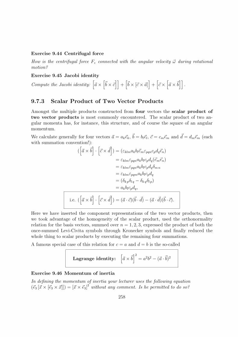
Exercise 9.44 Centrifugal force

How is the centrifugal force Fz connected with the angular velocity ~ω during rotationalmotion?

Exercise 9.45 Jacobi identity

Compute the Jacobi identity:[~a×

[~b× ~c

]]+[~b× [~c× ~a]

]+[~c×

[~a×~b

]].

9.7.3 Scalar Product of Two Vector Products

Amongst the multiple products constructed from four vectors the scalar product oftwo vector products is most commonly encountered. The scalar product of two an-gular momenta has, for instance, this structure, and of course the square of an angularmomentum.

We calculate generally for four vectors ~a = ak~ek, ~b = bl~el, ~c = cm~em and ~d = dm~em (eachwith summation convention!):

([~a×~b

]·[~c× ~d

]) = (εklmakbl~emεpqncpdq~en)

= εklmεpqnakblcpdq(~em~en)

= εklmεpqnakblcpdqδmn

= εklmεpqmakblcpdq

= (δk pδl q − δk qδl p)= akblcpdq,

i.e. ([~a×~b

]·[~c× ~d

]) = (~a · ~c)(~b · ~d)− (~a · ~d)(~b · ~c).

Here we have inserted the component representations of the two vector products, thenwe took advantage of the homogeneity of the scalar product, used the orthonormalityrelation for the basis vectors, summed over n = 1, 2, 3, expressed the product of both theonce-summed Levi-Civita symbols through Kronecker symbols and finally reduced thewhole thing to scalar products by executing the remaining four summations.

A famous special case of this relation for c = a and d = b is the so-called

Lagrange identity:[~a×~b

]2

= a2b2 − (~a ·~b)2

Exercise 9.46 Momentum of inertia

In defining the momentum of inertia your lecturer uses the following equation(~e3 [~x× [~e3 × ~x]]) = [~x× ~e3]2 without any comment. Is he permitted to do so?

258

9.7.4 Vector Product of Two Vector Products

We conclude our discussion of multiple products with the vector product of two vectorproducts. First we decide to maintain the second inner vector product as long as possibleuntouched: [[

~a×~b]×[~c× ~d

]]=[εklmakbl~em ×

[~c× ~d

]]= εklmakbl

[~em ×

[~c× ~d

]]= εklmakbl

((~em · ~d)~c− (~em · ~c)~d

)= εklmakbl(dm~c− cm~d),

i.e.[[~a×~b

]×[~c× ~d

]]= (~a~b ~d)~c− (~a~b~c) ~d, i.e. coplanar with ~c and ~d.

Here we firstly have replaced the first inner vector product by its components, then wetook advantage of the homogeneity of the vector product, afterwards we have developedthe nested vector product according to Grassmann, executed the projection on the com-ponents and finally reached triple products as coefficients of both the factor vectors of thesecond vector product, in the plane of which the result must lie.

Worried about this apparent asymmetry, we calculate the same product once more, nowby maintaining the first inner vector product as long as possible untouched and otherwiseproceeding in full analogy to above:[[

~a×~b]×[~b× ~c

]]=[[~a×~b

]× εklmckdl~em

]= εklmckdl

[[~a×~b

]× ~em

]= εklmckdl

((~a · ~em)~b− (~b · ~em)~a

)= εklmckdl(am~b− bm~a),

i.e.[[~a×~b

]×[~c× ~d

]]= (~a~c ~d)~b− (~b~c ~d)~a, i.e. coplanar with ~a and ~b.

Therefore the product vector of the vector product of two vector products must necessarilylie on the mean straight line of the planes spanned by both the factor pairs of the twoinner vector products.

259

Figure 9.28 : Vector product of two vector products

To have an overview we gather together the relations for the various multiple products:

With (~a ·~b) = akbk,[~a×~b

]= εklmakbl~em and (~a~b~c) :=

([~a×~b

]· ~c)

= akblcmεklm

there holds: [~a×

[~b× ~c

]]= (~a · ~c)~b− (~a ·~b)~c([

~a×~b]·[~c× ~d

])= (~a · ~c)(~b · ~d)− (~a · ~d)(~b · ~c)[[

~a×~b]×[~c× ~d

]]= (~a~b ~d)~c− (~a~b~c)~d = (~a~c ~d)~b− (~b~c ~d)~a

Thus we have reduced all multiple products into scalar, vector and triple products. Theonly thing remaining to do is to clarify how these three kinds of products behave underchanges of the coordinate system. To accomplish this we need a relation concerning thedeterminant of a transformation matrix, the determinant formula which we will obtain inthe following insert.

260

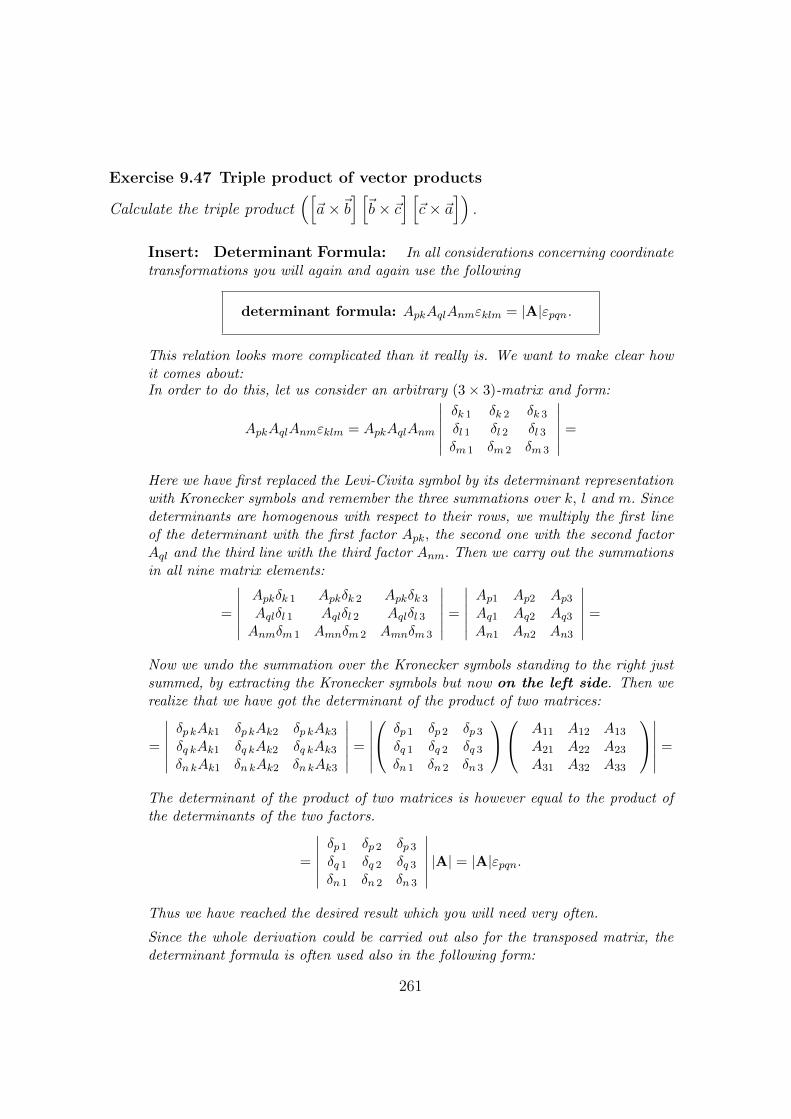
Exercise 9.47 Triple product of vector products

Calculate the triple product([~a×~b

] [~b× ~c

] [~c× ~a

]).

Insert: Determinant Formula: In all considerations concerning coordinatetransformations you will again and again use the following

determinant formula: ApkAqlAnmεklm = |A|εpqn.

This relation looks more complicated than it really is. We want to make clear howit comes about:In order to do this, let us consider an arbitrary (3× 3)-matrix and form:

ApkAqlAnmεklm = ApkAqlAnm

∣∣∣∣∣∣δk 1 δk 2 δk 3


∣∣∣∣∣∣ =

Here we have first replaced the Levi-Civita symbol by its determinant representationwith Kronecker symbols and remember the three summations over k, l and m. Sincedeterminants are homogenous with respect to their rows, we multiply the first lineof the determinant with the first factor Apk, the second one with the second factorAql and the third line with the third factor Anm. Then we carry out the summationsin all nine matrix elements:

=

∣∣∣∣∣∣Apkδk 1 Apkδk 2 Apkδk 3

Aqlδl 1 Aqlδl 2 Aqlδl 3Anmδm 1 Amnδm 2 Amnδm 3

∣∣∣∣∣∣ =

∣∣∣∣∣∣Ap1 Ap2 Ap3Aq1 Aq2 Aq3An1 An2 An3

∣∣∣∣∣∣ =

Now we undo the summation over the Kronecker symbols standing to the right justsummed, by extracting the Kronecker symbols but now on the left side. Then werealize that we have got the determinant of the product of two matrices:

=

∣∣∣∣∣∣δp kAk1 δp kAk2 δp kAk3

δq kAk1 δq kAk2 δq kAk3

δnkAk1 δnkAk2 δnkAk3

∣∣∣∣∣∣ =

∣∣∣∣∣∣ δp 1 δp 2 δp 3

δq 1 δq 2 δq 3

δn 1 δn 2 δn 3

A11 A12 A13

A21 A22 A23

A31 A32 A33

∣∣∣∣∣∣ =

The determinant of the product of two matrices is however equal to the product ofthe determinants of the two factors.

=

∣∣∣∣∣∣δp 1 δp 2 δp 3

δq 1 δq 2 δq 3

δn 1 δn 2 δn 3

∣∣∣∣∣∣ |A| = |A|εpqn.Thus we have reached the desired result which you will need very often.

Since the whole derivation could be carried out also for the transposed matrix, thedeterminant formula is often used also in the following form:

261

εklmAkpAlqAmn = |A|εpqn.

It is important that our determinant formula ApkAqlAnmεklm = |A|εpqn can be

looked at in an entirely different way: The Levi-Civita symbol, as a quantity with

three indices, can be considered also as a tensor of third order, and the left side

of our formula as εpqn, i.e. as a representation of the 27 tensor components in the

transformed coordinate system: for each index one transformation matrix. Thus

viewed, εpqn = |A|εpqn means the rotation invariance of the tensor components, i.e.

the ± ones and the zeros are in every coordinate system the same! In addition to this

fact there comes from |A| a minus sign for reflections. Thus we are dealing with

a pseudotensor. Correspondingly you will encounter the the Levi-Civita symbol,

being totally antisymmetric under exchange of each two indices, under the name

“numerically rotation invariant pseudotensor of third order”.

9.8 Transformation Properties of the Products

9.8.1 Orthonormal Right-handed Bases

After having got both products of two vectors we are able to characterize our originalcoordinate system S with its origin O in an elegant manner: Our basis vectors ~ek withk = 1, 2, 3 form an OrthoNormal Right-handed Basis (:ONRB), i.e. they:

are 1) orthonormal: (~ek · ~el) = δk lform a 2) right-handed system: [~ek × ~el] = εklm~emand are 3) complete: ~ek) (~ek = 1.

Besides this we consider with the same origin O = O in addition an other coordinatesystem S whose basis vectors ~ ke with k = 1, 2, 3 can be obtained from the old basisvectors by a linear transformation matrix A:

basis transformation: ~ek = Akl~el

We get the elements of the (3 × 3)-transformation matrix Akl = (~ ke · ~el) = cos∠(~ek, ~el)through scalar multiplication with ~el.

Now, physicist are interested in the following question: What kinds of matrices arepermitted, if the new basis shall form once again an ONRB?

262

9.8.2 Group of the Orthogonal Matrices

In order to answer that question we first treat orthonormality. The following relation isrequired to hold:δp q = (~ep · ~eq) = (Apk~ek · Aql~el) = ApkAql(~ek · ~el) = ApkAqlδk l = ApkAqk = ApkA

Tkq, i.e.

δp q = ApkATkq

Therefore, only matrices with the following property are permitted A AT = 1 or A−1 =AT . Mathematicians call these matrices orthogonal. From their nine matrix elementsonly three real numbers are independent because of the six constraint equations:

A2p1 + A2

p2 + A2p3 = 1 for p = 1, 2, 3 and

Ap1Aq1 + Ap2Aq2 + Ap3Aq3 = 0 for p 6= q = 1, 2, 3.

With respect to matrix multiplication, the orthogonal matrices form a group called O(3)which of course can not be Abelian, since we have found the multiplication of matrices ingeneral not to be commutative:

To verify the group property we consider first the product Ckl = BkpApl of two orthogonalmatrices A with ApnAqn = δp q and B with BkpBlp = δk l and calculate:

CknCln = BkpApnBlqAqn = BkpBlqδp q = BkpBlp = δk l

meaning the product of two orthogonal matrices is again orthogonal.Furthermore the associative law holds true as for every matrix multiplication:

C(B A) = C B A = (C B)A.

Exactly one unit element exists, since the unit matrix 1 is orthogonal because from1T = 1 it follows that 1 · 1T = 1 1 = 1 :

∃! unit element 1 : δkmAml = Akl = Akmδml for all A ∈ O(3).

For multiplication of a matrix A from the left or from the right with the unit matrix 1one obtains again the old matrix.

And an unambiguously determined inverse exists for every orthogonal matrix A, namelythe transposed matrix. For this was precisely the orthogonality condition:

263

∀A ∈ O(3) ∃! Inverse A−1 = AT : A AT = 1

The necessary condition for the existence of an inverse |A| 6= 0 is fulfilled, since fromAAT = 1 there follows for the determinant

|AAT | = |A||AT | = |A|2 = |1| = 1

|A| = ±1 6= 0.

With this, all group properties of orthogonal matrices are proven. From the determinantwe see furthermore that two kinds of orthogonal matrices exist: those with determinant+1, the rotations, and those with determinant −1. The latter are just the reflections.

The defining equation for the orthogonal matrices ApkAqk = δp q opens up a fully differentview on our Kronecker symbol: If we include on the left side a superfluous δ with afurther summation, we obtain: ApkAqlδk l = δp q. If we regard the Kronecker symbol,

because of its two indices, as a second order tensor, we find on the left side δpq, i.e. thenine elements of this tensor transformed to the new coordinate system: for each index atransformation matrix. Thus the entire equation δpq = δp q means the invariance of thematrix elements under rotations and reflections, i.e. the ones and zeros are unchanged inevery coordinate system and stay at the same position: The Kronecker symbol, symmetricagainst interchanging the two indices, is from a higher point of view a “numericallyinvariant tensor of second order”. You will frequently encounter it later on underthis name.

9.8.3 Subgroup of Rotations

Distinguished by having the determinant +1 the rotations form a subgroup of the groupO(3), the so-called special orthogonal group SO(3), since obviously (+1)(+1) = +1.

After these anticipatory discoveries, we want to investigate further how the orthogonalmatrices, allowed for the transformations of coordinate systems, may be further restrictedby the demand that the new basis vectors form again a right-handed system. Thatwill be the case if the following equation holds true:

εpqn~en = |A|εpqn~en.

264

In order to prove this let us consider

εpqn~en =[~ep × ~eq

]= ApkAql [~ek × ~el] = ApkAqlεklm~em = ...

After these calculational steps already known to us using the homogeneity of the vectorproduct, an unusual but important step now follows: We introduce in addition to the threesummations hidden in the Einstein convention over k = 1, 2, 3, l = 1, 2, 3 and m = 1, 2, 3a fourth one by inserting a Kronecker symbol which seems at first sight superfluous, andsum over r = 1, 2, 3:

... = ApkAqlεklmδmr~er = ...

The 1 introduced through the Kronecker symbol is now replaced by 1 = A AT , i.e.δmr = AnmAnr with our orthogonal transformation matrix A :

... = ApkAqlεklmAnmAnr~er = ApkAqlAnmεklmAnr~er = ...

After exchanging the numbers εklm and Anm we reach an expression which allows us touse the determinant formula ApkAqlAnmεklm = |A|εpqn derived earlier:

... = |A|εpqnAnr~er = |A|εpqn~en

Therefore, if our new basis shall be again a right-handed system, we must permit onlythose transformation matrices whose determinant is |A| = +1, i.e. only elements of thesubgroup SO(3) of the rotations. This is, however, just what we have seen in anexample at the beginning of this chapter: The parity transformation changed a right-handed coordinate system into a left-handed one, and so do all other transformationscontaining a reflection. The presence of coordinate reflections is reliably detected by thenegative determinant.

9.8.4 Transformation of the Products

At the end of this course we want to check how our products of vectors transform underrotations and reflections of the coordinate system:

We know already that the components ak of a vector ~a, which emerged from a displacementas projections onto the coordinate axes ak = (~a · ~ek) transform as do the basis vectorsthemselves:

ak = (~a · ~ek) = (~a · Akl~el) = Akl(~a · ~el) = Aklal,

thus

ak = Aklal.

265

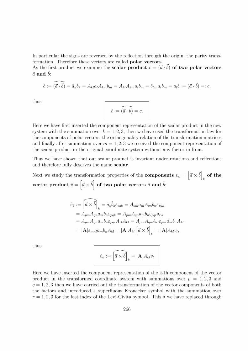
In particular the signs are reversed by the reflection through the origin, the parity trans-formation. Therefore these vectors are called polar vectors.As the first product we examine the scalar product c = (~a ·~b) of two polar vectors

~a and ~b:

c := (~a ·~b) = akbk = AklalAkmbm = AklAkmalbm = δl malbm = albl = (~a ·~b) =: c,

thus

c := (~a ·~b) = c.

Here we have first inserted the component representation of the scalar product in the newsystem with the summation over k = 1, 2, 3, then we have used the transformation law forthe components of polar vectors, the orthogonality relation of the transformation matricesand finally after summation over m = 1, 2, 3 we received the component representation ofthe scalar product in the original coordinate system without any factor in front.

Thus we have shown that our scalar product is invariant under rotations and reflectionsand therefore fully deserves the name scalar.

Next we study the transformation properties of the components vk =[~a×~b

]k

of the

vector product ~v =[~a×~b

]of two polar vectors ~a and ~b:

vk :=[~a×~b

]k

= apbqεpqk = ApmamAqnbnεpqk

= ApmAqnambnεpqk = ApmAqnambnεpqrδr k

= ApmAqnambnεpqrArlAkl = ApmAqnArlεpqrambnAkl

= |A|εmnlambnAkl = |A|Akl[~a×~b

]l=: |A|Aklvl,

thus

vk :=[~a×~b

]k

= |A|Aklvl

Here we have inserted the component representation of the k-th component of the vectorproduct in the transformed coordinate system with summations over p = 1, 2, 3 andq = 1, 2, 3 then we have carried out the transformation of the vector components of boththe factors and introduced a superfluous Kronecker symbol with the summation overr = 1, 2, 3 for the last index of the Levi-Civita symbol. This δ we have replaced through

266

two orthogonal transformation matrices and combine the three matrices A with help of thedeterminant formula ApkAqlAnmεklm = |A|εpqn into the determinant, and finally writtenthe vector product in terms of the old vector product in the old untransformed system.

Thus, it follows that the vector product transforms under rotations like a displacementas a vector, but under reflections because the determinant |A| = −1 introduces anextra minus sign, the vector product is reflection invariant. Vectors with this propertyare called axial vectors, and in fact all vectors built as vector products of two polarvectors appearing in physics are reflection invariant. As we have seen, all of these arerelated to rotational processes and represent in some sense - unlike the direction arrowof displacement vectors - a turning event which does not change when looked at in amirror. The following figure attempts to display this.

Figure 9.29: Turning circle and displacement arrow under a reflection through the origin

Exercise 9.48 Polar and axial vectors

Sort the following examples of physical vectors in two boxes according to their behaviorunder reflections, on the one hand the polar vectors and on the other hand the axial ones:

267

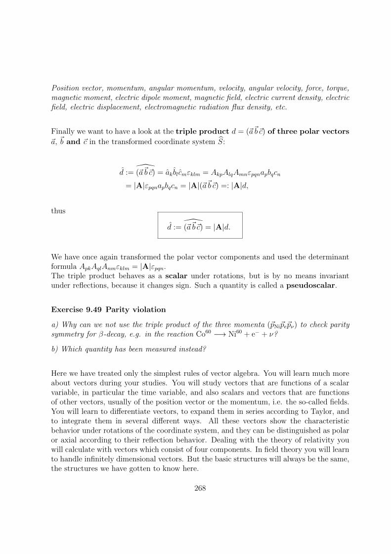
Position vector, momentum, angular momentum, velocity, angular velocity, force, torque,magnetic moment, electric dipole moment, magnetic field, electric current density, electricfield, electric displacement, electromagnetic radiation flux density, etc.

Finally we want to have a look at the triple product d = (~a~b~c) of three polar vectors

~a, ~b and ~c in the transformed coordinate system S:

d := (~a~b~c) = akblcmεklm = AkpAlqAmnεpqnapbqcn

= |A|εpqnapbqcn = |A|(~a~b~c) =: |A|d,

thus

d := (~a~b~c) = |A|d.

We have once again transformed the polar vector components and used the determinantformula ApkAqlAnmεklm = |A|εpqn.The triple product behaves as a scalar under rotations, but is by no means invariantunder reflections, because it changes sign. Such a quantity is called a pseudoscalar.

Exercise 9.49 Parity violation

a) Why can we not use the triple product of the three momenta (~pNi~pe~pν) to check paritysymmetry for β-decay, e.g. in the reaction Co60 −→ Ni60 + e− + ν?

b) Which quantity has been measured instead?

Here we have treated only the simplest rules of vector algebra. You will learn much moreabout vectors during your studies. You will study vectors that are functions of a scalarvariable, in particular the time variable, and also scalars and vectors that are functionsof other vectors, usually of the position vector or the momentum, i.e. the so-called fields.You will learn to differentiate vectors, to expand them in series according to Taylor, andto integrate them in several different ways. All these vectors show the characteristicbehavior under rotations of the coordinate system, and they can be distinguished as polaror axial according to their reflection behavior. Dealing with the theory of relativity youwill calculate with vectors which consist of four components. In field theory you will learnto handle infinitely dimensional vectors. But the basic structures will always be the same,the structures we have gotten to know here.

268

Beyond scalars and vectors, in some areas of physics you will meet tensors of secondorder, e.g. the momentum of inertia, the stress tensor and the electric quadrupol moment.In four-dimensional space-time the electromagnetic fields together form a second-ordertensor. The transformation theory of tensors has much in common with the transformationtheory of vectors, and our considerations here have prepared you for this more advancedmaterial. I do hope you will enjoy it!

269

mathematical preparation course before studying physicshefft/vk_download/vk1e.pdf · mathematical...

Documents