by

URI WEISERand ‘

ALAN L. DAVIS

UUCS - 80 - 111

MATHEMATICAL REPRESENTATION FOR VLSI ARRAYS

Department of Computer Science University of Utah

Salt Lake City, Utah 84112

SEPTEMBER 1980

This work was supported under the Data Driven Research Project grant provided by Burroughs Corporation.

i

1 INTRODUCTION 12 MATHEMATICAL PRESENTATION OF SEQUENCES 5

2.1 THE D OPERATOR 53 ONE DIMENSIONAL ARRAYS 9

3.1 MATRIX-VECTOR MULTIPLICATION 93.2 SOLVING TRIANGULAR LINEAR SYSTEMS 12

4 TWO DIMENSIONAL ARRAYS 144.1 BAND MATRIX MULTIPLICATION 15

4.1.1 General approach 154.1.2 Construction of the network. 17

4.2 SOLVING A SET OF TRIANGULAR LINEAR SYSTEMS 214.2.1 CASE 1: A X = Y, where A is a triangular band matrix, 21

and X and Y are full matrices '4.2.2 CASE 2: A X = Y , where A, X and Y are all band matrices 22

5 CONCLUSIONS 25I. Number of multiplications in Matrix Multiplication 26

Table of Contents

i l

Figure 1: Two steps Transformation 2Figure 2: The delay element [eq. Cl)]- - 5Figure 3: The system z=F(x,y) 6Figure 4: row feeding of full matrix B 7Figure 5: Multiplication of a band matrix by a vector [eq. (4)]. 9Figure 6: Matrix-vector multiplication network [eq. (7)]. 10Figure 7: The basic block P 11Figure 8; Matrix-vector multiplication network using the basic block P 11

[eq. (7)].Figure 9: Triangular linear system network [eq. (10)]. 12Figure 10: Triangular linear system network using the basic block P [eq. 13

(10)].Figure 11: Triangular linear system network using the basic block P [eq. 13

. (13)].Figure 12: Band matrix multiplication 15Figure 13: Wavefront £ and D[2] 16Figure 14: Orientation of A and X. 17Figure 15: The stream of data of the partial results of Y 18Figure 16: Band matrix multiplication, output Y in colunns [eq. (17)]. 19Figure 17: Band matrix multiplication, producing the output Y in colunns 20

[eq. (20)].Figure 18: Solution for a set of simultaneous equations, when A is a 22

triangular band matrix and X and Y are full matrices [eq. (23)].

Figure 19: Solution for a set of simultaneous equations, when A, X and Y 23 are band matrices, using the basic block P [eq. (27)].

Figure 20: Processor array for solving a set of triangular linear 24 systems, when A, X and Y are band matrices, using the basic block P [eq. (30)].

Figure 21: Number of multiplications needed to calculate the set Q 26

List of Figures

1

This paper introduces a methodology for mapping algorithmic description

into a concurrent implementation on silicon. This methodology can help in the

solution of important problems using a new technique for the representation of

highly parallel networks. This new approach for the representation of

computational networks was inspired by the systolic array approach [H.T. Kung

& Leiserson 78], and by the linear approach to computational networks [Cohen

78]. It creates tools which will enable the creation of new high performance

implementations as well as verification tools. This approach is more complex

than the linear approach [Gill 66, Cohen 78], but can also be used to verify

computational networks.

Speedup in sequential machines can only be achieved by increasing component

speeds. There is however no reason why implementation of a particular circuit

should be constrained to a sequential hardware algorithm. Concurrency can be

exploited in two fundamental ways:

1. Take advantage of the inherently independent operations which can be split up and performed at the same time in parallel, and

2. Take advantage of computations which can be performed in a pipelining fashion.

For the purpose of this paper we will refer to the concurrent processing of

independent operations at the same time as horizontal concurrency. We will

also refer to the pipelined style of concurrent evaluation as vertical

concurrency. Vertical concurrency can be effective when the inputs are

recurrent and when the computation is similar for the recurring groups of

input elements. It subsequently will be shown that this pipelined style of

computation can be implemented by spreading the computation in the time domain

or in the space domain. Horizontal concurrency is effective when a

computation can be decomposed into subcomputations which are independent and

can run at the same time. The class of problems which can be decomposed into

subcomputations and for which the input data set is inherently recurrent can

be implemented very efficiently in hardware. This paper presents a

1 INTRODUCTION

2

mathematical method for dealing with this class of problems.

The complexity of some of the problems is such that it is hard to exploit

vertical and horizontal concurrency using intuition as the only design tool.

A methodology for transforming the description of the problem into hardware

implementation would be very useful and could help in the design of new fast

and efficient circuits. A definition of the rules for this method could be

used as a basis for an automatic way to implement hardware from the formal

description of the problem. In order to achieve an optimal design it is

necessary to define the design objectives. The design objectives can be:

efficiency, delay, throughput, speed, parts count, modularity, power,

communication locality, etc.

The transformation from the description of the problem to the special

purpose hardware can be pursued in two steps:

- Mathematical transformation of the definition of the problem, where

the result is a final mathematical equation which can be mapped directly into hardware. This will be referred to as the mathematical transformation step.

- Transformation from the final mathematical form into hardware. This

will be referred to as the mapping step.

Mathematical MappingO ________ trans formation_____ q q

Mathematical Final Hardwaredefinition of equationthe problem

Figure 1 : Two steps Transformation

The desired result of the first step should be such that the subsequent

mapping transformation will result in a circuit of high performance. The

final circuit can then be evaluated against the design objectives.

The VLSI trend towards simple repetitive components, and the trend to

exploit maximum concurrency to increase computational speed, motivates the

division of a system into modular parts (similar to cellular array). A

cellular array can be constructed out of independent elements exhibiting local

3

control. This approach will result in a modular and expandable system. The

temporal control of these array like networks can be done in either an

asynchronous or a synchronous fashion. Synchronous control is inherently

simpler in a logical sense but there are some physical problems associated

with distributing clock signals over long paths on silicon. The primary

problem is that maintaining the clock skew to be within an acceptable bound

for the synchronous system becomes difficult as the system size is expanded.

The limitations of synchronous VLSI systems are made worse as the feature size

scales down and chips become larger. This suggests an asynchronous approach

where the modular elements are independently timed or self-timed [Seitz 79].

It is reasonable to view these self-timed elements as autonomous elements

which function internally as synchronous circuits, but communication is

performed between modules in an asynchronous manner. This can be done

reliably if the clocks of the synchronous modules are stopped synchronously

and then restarted asynchronously in response to input data arriving from

other modules. This data-driven approach has been demonstrated in the DDM1

machine [Davis 77].

Seitz [Mead&Conway 80] has shown that a reasonable physical area for

encapsulating a synchronous module on silicon corresponds to an equipotential

region. An equipotential region is an area over which a signal can be

propagated in a time less then or equal to a single transistor switching time.

A signal transition which occurs at a rate faster than the switching time of a

single transistor is not observable by the logical elements of the circuit.

This implies that the voltages observed at all points along a path in an

equipotential region can be considered to be equal by the logical elements of

the circuit. Seitz has also shown that the maximum area of an equipotential

region scales down roughly linearly with the feature size. At the projected

limit of the feature size, the maximum number of components that could reside

in an equipotential region would only be able to perform a few relatively

simple arithmetic operations. This implies that the elements of a cellular

array should be designed so that they are required to perform operations on

4

the order of relatively simple arithmetic operations.

H.T. Kung [H.T. Kung & Leiserson 78] and S.Y. Kung [S.Y. Kung 80] have

described methods for combining very simple elements into a system which can

perform several matrix computations. In this paper, a mathematical approach

for this class of computational networks is shown. This mathematical approach

enables checking for correctness and accuracy of these computational networks,

and aids in the generation of implementation schemes which exhibit both a high

computation rate and a low delay. This mathematical representation can also

be used as' a tool which facilitates the search for new computationally

equivalent structures. An intuitive view of the operation of these

computational networks is that they are cellular logic arrays through which

streams of input data pass and are transformed by the array elements to

generate the desired result streams. These streams, which will be defined

more formally in the next section, follow directed paths through the

computational network and do not change direction as they pass through the

network logical elements. These logical element will subsequently be referred

as processors or as basic blocks. It is important to note that these

processors are not general purpose but are specialized logic elements which

are typically small and simple.

In section 2, the basic mathematical concepts are given along with some

rules and definitions which are used later in the discussion. Section 3

presents one-dimensional array implementations of two problems which are given

as simple examples demonstrating the methodology. Section 4 uses the same

basic technique, but presents some additional concepts and solutions for two

dimensional array problems.

Tne main theme is to show a new direction in the representation of

computational networks. This paper presents some initial results describing

the solution of some important problems using this new technique for the

representation of highly parallel networks. The technique represents an

initial step in finding a method to map an algorithmic description onto a

5

2 MATHEMATICAL PRESENTATION OF SEQUENCES

The mathematical notation used in this paper encompasses the use of

pipelining, concurrency of computation and flow of data in an array of simple

processors. The array of processors which performs the computation is

connected by regular fixed communication links, and can therefore form an

array on silicon.

. This systolic array approach [H.T. Kung & Leiserson 78], uses the idea

that time and space interleave. The processors can be viewed either as an

asynchronous system (data driven) or as a synchronous system. For simplicity

in exposition, the following description will view the operation of these

arrays as synchronous. This synchronous view implies a time metric which can

be conceptually divided into clocks, time steps, or cycles. The duration of a

time step is dependent upon the actual implementation but logically

corresponds to the maximum time required by a processor to produce its outputs

from a given input set and communicate these results to their respective

destinations.

2.1 THE D OPERATOR

D will be defined as a delay operator. When X is a data element at s

particular point in a computational network, D[X] is defined as the data

element that was at the same point on the previous time step.

A sequence X (1 ) ,X (2 ) ,X (3 ) , . . • ,X(i-1) ,X (i ) ,X (i+ 1 ) is defined, where X(i)

precedes the arrival of X(i + 1) by one time step. When the D operator is

applied to this sequence as described by Cohen [Cohen 78], the following

relationship holds:

D[X( i)]=X(i-1) (1)

Figure 2 shows the network represented by Equation (1 ) . The D operator may be

implemented by a simple register. Manipulations of mathematical expressions

containing the D operator are governed by two rules. Rule 1 is merely a

recursively expressed form of Equation (1 ) . Rule 2 describes the commutative

concurrent im plem entation on s i l i c o n .

6

X ( i ) X (i- l )D

Figure 2: The delay element [eq. ( 1 )] ;

and distributive properties of the D operator.

Rule 1: A recursive definition of the D operator.

Dn[X(i)]=D{Dn-1 [X (i)]}

Using this recursive definition it is possible to derive:

Dn[X(i)]=X(i-n)

Rule 2: The commutativity of delay and operation.

This paper will deal with functions which obey the equation:

Di[F(x,y)]=F(Di[x],Di[y])

When F(x,y) is a function such that for every x and y there exists an

output F (x ,y ), and when the set *2,Y2 preceeds the set x-],yi at the input

terminals of the system, then F(x2 ,y2) proceeds F (x 1 tYi) that is:

DC x2]=xiD[y2]=yiD[F(x2 ,y2 )]=F(xi ,y-|)

(2)

F(x,y)

z

Figure 3 : The system z = F (x ,y )

7

Proof:

Substitution of x1f y-j with D[x2 l, D[y2] in equation (2) results in Rule 2:

DCFCx^y^lsFCDCx^.DCy!]) (3)

Rules 1 and 2 are general rules which can be applied to all sequences. For

the purpose of this paper, two more rules will be defined which apply to a

particular case of band matrices^ (Rule 3)t and full matrices (Rule 4 ) . The

use of band matrices does not limit the generality of these ideas and can be

easily extended to full matrices.

Rule

If a band matrix A is fed into (or is an output of) a system through s+r+1

terminals, where each terminal receives (or produces) a sequence of elements

along one distinct diagonal of the band matrix [i.e A (i ,j ) is followed by

A (i+ I ,j+ 1 ) throughout the computation] then:

Dk[A(i,j)]=A(i-k,j-k)

This rule describes the pipelined nature of such an implementation for

matrix algorithms.

Rule 4:

When a full matrix B, with a limited number of colunns (M) and an arbitrary

number of rows, is being fed row by row as shown in Figure 4.

the delay D on each of the inputs obeys the rule:

DJ[B(I,J)]=B(I- j,J)

Remark: In the next two sections, final equations will be derived for

several problems. The final equation represents the end point of the

mathematical transformation of the equation which initially defines the

^A band matrix is a matrix where: A (i ,j )= 0 , for i-j>s or j-i>r. The band

width is r+s+1 (see Figure 5 ).

8

BC 4 ,1) B ( 3 , 1) B (2 ,1) BC1 , 1 ) ----- >

B(M,2) B (3 ,2 ) B (2 ,2) B (1 ,2 ) ----- >

B(M,3) B ( 3 , 3) B (2 ,3 ) B ( 1,3) ----- >

• • • •• • • •

B(M, I) B (3 , I ) B(2 , I) B (1 , I) ------>

B(M,M) B(3 ,M) B(2,M) B(1,M) ----- >

Figure M: row feeding of full matrix B

problem. These final equations are clearly not unique as the process of

mathematical transformation can be continued indefinitely. From these final

equations it is possible to construct the computational networks. The final

equation represents a snap-shot of the network. This snap-shot is an

instantaneous view of the state of the computational network. The final

equation describes the relation between sets of inputs and sets of outputs of

the computational network. Typically the output terms are on the left hand

side of the final equation and the input terms are on the right hand side.

The set of input terms have to be a time independent set where:

Definition: A Time independent set (Tl set) is a set, whose elements can not be represented as elements of the same stream of data.

A time dependent set (TD set) is a set with elements which can be represented as elements of one stream of data.

A stream of data is the set of elements along a directed path through nodes of the computational network. Here a node can be

either a delay or a single operation followed by a delay.

A time dependent form (TD form) is a term describing the time

dependent set, without using the D operator.

______________ A space dependent form (SD form) factors the description of

the time dependent set into a product of a time independent

set and a delay.

Example: Consider a band matrix A, where the sequences are of the form

described in rule 3 . A set in the form A(I,J-m), for varying m, is a time

Definition:

Definition:

Definition:

Definition:

9

independent set because it represents elements from different streams of data.

An input set of the form A(I-m,J-ra), for varying m, is a time dependent set

because it represents elements of the same stream of data. This A(I-m,J-m)

set is a delayed version, in time or in space, of A (I ,J ) . The view of this

set in the time dependent form [A(I-m,J-ra)] is that by waiting at one point in

space the members of the set can be viewed over time. In the space dependent

form (Dm[ A (I ,J ) ] ) , it is possible to stop the computational network at a point

in time (snap-shot) and view the members of the set [A(I-m,J-m)] over a

directed path' in space.

3 ONE DIMENSIONAL ARRAYS

One-dimensional arrays have been used to implement circuits such as F .I .R .

filters, polynomial multiplication and division, SAR data processing [Cohen

78]. Further applications are matrix-vector multiplication, solving triangular

linear systems, and Discrete Fourier Transforms [H.T. Kung & Leiserson 78].

In this section the mathematical rules mentioned in section 2, will be used to

create an efficient network for matrix-vector multiplication, and to create a

network which is capable of solving triangular linear systems which are

represented by triangular band matrices, (see Figure 5 where s=0).

3.1 MATRIX-VECTOR MULTIPLICATION

We consider the problem of multiplying a band matrix A by a vector

X. Matrix A has a band width of N=r+s+1 (see Figure 5 ). The elements in the

product Y, can be computed by:

n+s

Y(n) = 2 " A(n,m)X(m) (4)m=n-r

By choosing m=n+s-j, which implies j=n+s-m, and by inverting the order of the

summation. Equation (4) becomes:

s+r

Y (n)r^A(n ,n+s- j)X(n+s- j) (5)j = 0

The computational network represented by Equation (5 ) , requires s+r+1

additions for each Y(n) every time step. By distributing the summation

10

s= l*

A (1, 1) A (1 ,2) 0 X(1) Y(1)

A (2 ,1) A (2 ,2) A(2,3) X(2) Y(2)

A(3.1) A(3.2) A (3 .3) A (3 .4) X X(3) - Y(3)

A (4 ,2) A (4 ,3) A (4 ,4) A (4 ,5) : :

0 A(5,3) A (5 ,4) •

A(5.5)•

4

Figure 5: Multiplication of a band matrix by a vector’ [eq. (4 )] .

[Cohen 78] over the space domain, it is possible to obtain a more parallel

solution. Equation ( 6 ) can be derived from Equation (5) using rules 2, and 3t

shows this distribution.

Y(n) = 5^D^[A(n+j,n+s)X(n+s)] (6)

j=0

Tnis form holds for all values of n. The term delays the product

A(n+j,n+s)X(n+s). Equation (6) can also be written in the form:

Y(n)=A(n,n+s)X(n+s)+D{A(n+1,n+s)X(n+s)+D[A(n+2,n+s)X(n+s)+D(. . ) ] } (7)

*The computational network represented by Equation (7 ) is shown in Figure 6 .

A(n+s+r,n+s) A(n+s+r-l,n+s)

'-E

-A

A(n+1,n+s) I

T "

A(n,n+s) i ' i

\ r nY (n) Y(n-l)

Figure 6 : Matrix-vector multiplication network [eq. (7)]<

A basic repeated block P can now be defined as shown in Figure 7. Streams

of data (as defined in section 2 . 1 ) can flow only in the direction labeled x,

a, and y in Figure 7* Using this basic block, every multiplication is followed

11

by an addition operator and a delay element.

x'=D[x]

a ’=D[a]

y ’=D[y+ax]

Figure 7: The basic block P

The basic block P will be used throughout this paper. In some cases only a

subset of the inputs and outputs of P will be used. By using the block P to

construct the network shown in Figure 6, the network of Figure 8 can be

generated which represents a delayed version of Equation (6 ) :

s+r

Y(n-1)=D[Y(n)] = ̂ D j+1[A (n+j,n+s)X (n+s)] (8)

j=0

A(n+s+rfn+s) A(n+s+r-l,n+s) A(n+s+r-2,n+s) A(n,n+s)

Figure 8: Matrix-vector multiplication network using

the basic block P [eq. (7 )] .

In a single time step one colunn of matrix A and one element of vector X are

fed into the network. All of the elements in the pipe perform an operation

every time step, resulting in high throughput and high efficiency.

The result shown in Figure 8 is a simple example of the general

mathematical method, however an intuitive approach could lead to the same

result. This is primarily due to the inherent geometric simplicity of

matrix-vector multiplication.

12

3 .2 SOLVING TRIANGULAR LINEAR SYSTEMS

Unlike the matrix-vector multiplication algorithm, which can be intuitively

approached, the mathematical approach becomes more attractive when applied to

more complex problems such as solving triangular linear systems.

Let the vector X (Figure 5) represent the unknowns in a set of linear

equations. Let A represent the coefficient lower triangular band matrix (i .e

s=0). The elements of the main diagonal of A have to be non zero [ i .e .

A ( i ,i ) /0 for all i] . Let Y represent the result vector. Equation (6) gives the

result for Y (n ):

r

Y ( n ) = ^ Dj[A(n+j,n)X(n)]

j=0

Tne solution for A(n,n)X(n) is given by:

r (9)A(n,n)X(n) = {Y (n )- ^ Dj[A(n+j,n)X(n)]}

j=1

Letting B(n)=A(n,n)X(n) and by using Rule 1, Equation (9) can be

transformed into:

r (10)B(n)=Dr[Y(n+r)] + ̂ D j[{- A (n + j,n )[1 /A (n ,n )]}B (n )]

j = 1

The computational network represented by Equation (10) is shown in Figure

Figure 9: Triangular linear sy3tem network [eq. (10 )].

13

Figure 10 shows the same algorithm, implemented using the basic block P

defined in Figure 7. Using these blocks a delay is associated with each

multiplication as shown by:

[A (n+j,n )][1/A(n,n)]=D{[A(n+j+1,n+1) } 1/A(n+1,n+1) (11)

Using the association of Equation (1 1 ), Equation (10) becomes:

B(n)=Dr [Y(n+r)]+ $ ! DJ{D[-A(n+j+1,n+1)/A(n+1,n+1) ]B (n)}

j = 1

(12)

A (n+1,n+l)

Figure 10: Triangular linear system network using

the basic block P [eq. (10 )] .

Equation (12) implies the broadcasting of A(n+1,n+1). It is possible

however to construct a different but functionally equivalent computational

network with only limited broadcasting. The final equation of this limited

broadcasting network is given by Equation (13) and the corresponding network

is shown in Figure 11.

(13)X(n)=Dr [D{Y(n+r+1)/A(n+r+1,n+r+1)}]-

r

' D>5[D{A(n+j+1 ,n+1 )Dr” J[ 1/A(n+r+1 ,n+r+1)] }X(n) ]

j=1

The throughput of these computational networks is such that one element of

the vector X is produced every time step. The number of blocks used to

1M

lA(n+r+l,n+r+l)

Figure 11: Triangular linear system network using

the basic block P [eq. (13)1-

construct these networks is 2r+1 or 2N-1 where N is the width of matrix A

(i .e . N=r+1, note that s=0 in this case). All of the elements in this network

are kept busy. The inputs for each time step is a colunn of matrix A, and one

element of vector Y. The network delay in Figure 9 is r+2 (for output X) and

is r+1 for the solution given in Figure 11.

Definition: Network delay is the longest acyclic path from an input to an output, and is measured in terms of the number of delay elements.

The delay can be easily seen in the final equation and is the highest power

of D in the equation.

M TWO DIMENSIONAL ARRAYS

Two dimensional array problems are much more complex than those which are

one dimensional. In order to exploit pipelining, the data has to flow in more

than one direction. H.T. Kung [H.T. Kung 4 Leiserson 78] has shown such a

computational network which performs matrix-multiplication for band matrices.

In this section two algorithms for this problem are given which are more

efficient than those presented by H.T. Kung. An algorithm for solving a set

of triangular linear systems is also presented.

15

U.1 BAND MATRIX MULTIPLICATION

U.1.1 General approach

Let A and X be band matrices with band widths f'l+si + i, and r2+S2+1

respectively; and let matrix Y be the product matrix of A and X (see Figure

12).

V a,-l •"W*

Figure 12: Band matrix multiplication

One strategy is to try to get one column of the matrix Y as an output of

the network in every time step. Y(J-n,J) will represent colunn J of matrix

Y. By changing n it is possible to get all the elements of this colunn [n will

vary from -r=-(r-|+r2 ) to s=si+s2 ]. In the general case:

k2 (14)Y(J-n,J) = ̂ “ A(J-n,k)X(k,J)

k=k1

For any specific n, k1 and k2 are the limits of the range of subscripts

which participate in the term. Equation (1U) can be rewritten as:

M (15)

Y(J-n,J)=£2 A(J-n,J-n-r1+j)X(J-n-r1+ j , J)

j=0

M+1=r^+s^+1 is the band width of matrix A. As was shown in section 3 .1 , the

distribution of the summation over the space domain will give:

{*<».«) ««,» «M)

- *(7,1) Aft.t) * 1 ,1 } Atl.i)

M

Y(J- n,J)=]^ DJ[A(J-n+j,J-n-r1+2j)X(J-n-r1+2j,J+j) j=0

(1 6 )

16

The term A, for varying j and n, is in a time dependent form, as was

defined in section 2. Multiplying the term A by D'HD--}] will change it to a

space dependent form. Note that D° for negative n and D“ J are essentially

predictions (negative delay). To overcome this problem term A will be

multiplied by Dr+n[D^“^] which is always a positive delay. X is also in a

time dependent form when j varies. Multiplying term X by will change this

term to a space dependent form as well. Since using the basic block P

requires that every multiplication must be followed by a delay, Equation (16)

must then be rewritten to include this delay in the case where j=0. These

arguments can be combined and mathematically represented as the final equation

(17 ).

M (17)D[Y(J- n,J)]=^Dj+ 1[DM-jtDr+n[A( j +r+Mtj +r+Sl+j )]}DM-j[X(j+s1_n+j tj+M)]]

Where:

D[Y(J-n,J)]=Y(J-n-1, J-1)

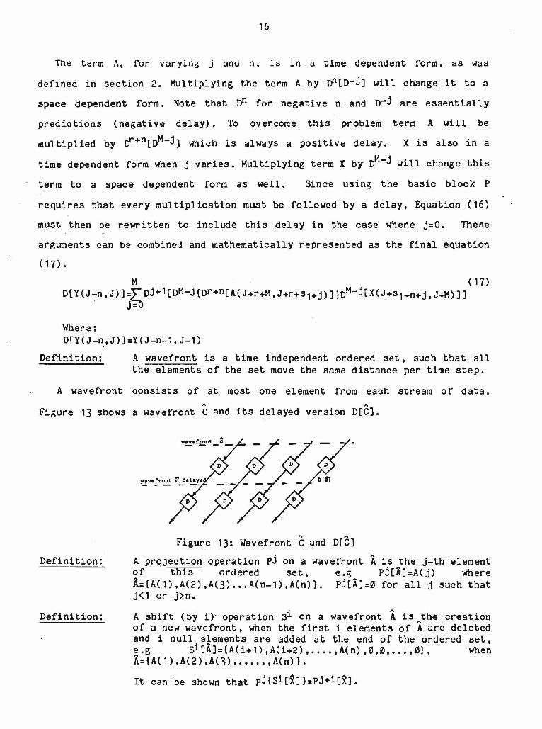
Definition: A wavefront is a time independent ordered set, such that all

the elements of the set move the same distance per time step.

A wavefront consists of at most one element from each stream of data.

^ A

Figure 13 shows a wavefront C and its delayed version D[C].

Definition:

D e f i n i t i o n :

Figure 13: Wavefront C and D[C]

A projection operation PJ on a wavefront A is the j-th element of this ordered set, e.g PJ[A]=A(j) where

H ={A (1 ),A (2 ),A (3 )...A (n - 1),A (n )} . PJ[A]=0 for all j such that j<1 or j>n.

A shift (by i) operation S* on a wavefront A is^the creation of a new wavefront, when the first i elements of A are deleted and i null elements are added at the end of the ordered set,e.g Si [A]={A(i+1) ,A (i+ 2 ) ----,A (n ) , 0 , 0 , . . . , 0 } , whenA={A( 1) ,A(2) ,A (3 ) ............A(n) } .

It can be shown that pj{Si[£]}=pj+i[£].

The 3et of elements A(J+r+M,J+r+s-|+j)for j=(0 to M) , will be defined a3

wavefront A, when A( J+r+M, J+r+s^) is the fir3t element of the set and

A(J+r+M,J+r+s.|+M) is the last. The set of elements X(J+si-n+j, J+M) for j=(0

to M) and where n=[-(r-i+r2) to s-|+s2], will be defined as wavefront X Mhen

X(J+M+r2+M,J+M) is the first element (with a zero value because

X(J+M-r2+i,j+M )=0 for all i>0) , and X(J-S2 ,J+M) is the last element of the set

( X(J+M-s2-i, J+M)=0 for all i>0 ) . Using Shift and Projection operations,

equation ( 1 7 ) can be written in the form:

M (18)D [ Y (J ^ n ,J ) ] = ̂ D j + 1 [ D M-j{P j(D»*+n[A])}DM- j { P M* - j ( s r + n [ x ] ) } ]

j=°

Where:

Dr+n[A] is the delayed wavefront and

Sr+n[A] is the shifted wavefront.

With respect to final equation (17 ), tT+n delays the wavefront A, andA A

delays a particular element of wavefront A, and similarly for wavefront X

( i .e . the subscripts of A and X are a function of j ) . delays the partial

result of Y in the direction of the stream of data Y, which passes through

addition operations and delay elements. Although it is possible to

reconstruct the network by using equation (18) we feel that some more tools

have to be developed to simplify the reconstruction of the network from the

final equation. Equation (17) will be used as a base for the reconstruction

of the network.

4 . 1 . 2 C o n s tru c tio n o f th e n e tw o rk .

Tne construction of the network is done in two steps. Using the final

equation ( 1 7 ) . step 1 deals with the relative orientation of the inputA A

wavefronts A and X. In step 2, the direction of the pipelined result stream Y

is constructed.

S te p 1 : O r ie n t a t io n o f A and X .

For j=M and r+n=0 [see Equation (17 )] . the element A1 =A( J+r+M, J+s-j+r+M) is

18

Figure 14: Orientation of A and X.

multiplied by the element X'=X(J+s^+M,J+M) as shown in Figure 14 at point 1.

For r+n=1, the wavefront A is delayed by one delay element. The element

D[A' ]=D[A( J+r+M, J+si+r+M) ], is a part of D[A]. and is multiplied, at point 2

of Figure 14, by the element X"=X(J+s1+M-1, J+M). X" as well as X' are elements

of the wavefront X. The same technique can be used for all values of n. This

step shows that the direction of the stream of data of A is parallel to the

wavefront X. In the same way it can be shown that the direction of the stream

A

of data of X is parallel to the wavefront A.

As a result of step 1, it is clear that the network will reside on a two

dimensional grid. A rectangular grid is attractive when the elements are the

basic blocks P, as shown in Figure 7.

Step 2: The direction of the pipelining of the result Y.

For the case where r+n=0 and for all j , the stream of data of the partialA

result of Y has to be at the same delay distance from the two wavefronts A and

X (see Figure 15). Delay distance is measured in terms of the number of delay

elements. For r+n=1, the path of Y(J+r-1,J) should be an equal delay distance

from D[A], and from the shifted wavefront X as shown by Equation (1 7 ). This

process can be proven inductively. Figure 15 shows the approach presented in

step 2.

The overall network, which can be constructed using these two steps is

shown in Figure 16, for the case where r-j = 2, s-|=2, r2=1, and S2=2. The result

19

wavefront X

N l\M-j *|delay on elements of X

delay on elements of A

direction ofstream of data

of partial result Y

-j-0 ■j-1 •j-2 j=M=3 „

r+n-0

--- j«M=3 }1=3 I r+n=*l

Figure 15: The stream of data of the partial results of Y

matrix Y is such that r=3 and s=4. The inputs at every time step are: one

column of X, and one row of A. The output is one column of Y on the network

outputs for every time step (or a row-column combination, when there are no

delay elements).

MJ+T+M.J+r+M**.)

, ______________________________________________________f X in colon okWt *

il,-

M N I X I

j x r v i x

X M X I N

\ X v C \

Figure 16: Band matrix multiplication, output Y in columns [eq. (17)]

The shaded elements, shown in Figure 16, function only as delay elements

and can be eliminated. Note that only the unshaded elements are needed,

20

th e re fo re m atrix m u lt ip l ic a t io n can be implemented using ( r i+s-j + i ) ( r 2+S2+1)

e lem en ts . I t i s p o s s ib le to show (Appendix I ) , th a t in order to produce, in

one tim e s te p , a s e t Q o f outputs co n ta in in g r+s+1 e lem en ts , where no two

elem ents are members o f the same d ia g o n a l, [ i . e Q can be one column or one row

o f the r e s u l t m atrix Y, e t c . ] the number o f m u lt ip l ic a t io n s needed i s

(r-|+ si + 1) (T2+S2+1) . Note th a t the nunber o f m u lt ip l ic a t io n s needed to produce

the se t Q in ons tim e ste p i s the same as the number o f b lo ck s P used in the

im p lem entation . S in ce the unshaded b lo ck s in F ig u re 16 produce the s e t Q in

one tim e s te p , t h i s im p lie s th a t t h is network i s optim al in e f f ic ie n c y .

The dashed arrow s in F ig u re s 16 and 17 p o in t in the d ire c t io n o f in c re a s in g

s u b s c r ip t s fo r X, A, and Y. Using a. s im i la r technique i t i s p o s s ib le to

c o n s tru c t a com putational network w hich perform s m atrix m u lt ip l ic a t io n . The

o n ly d if fe r e n c e between t h i s s t ra te g y and the former one i s th a t s-j_ j appears

in the s u b s c r ip t in Equation (15 ) in ste a d o f - r - i+ j.

M ( 1 9 )Y ( J - n , J ) = 5 ^ A ( J - n , J - n + s 1_ j ) x ( j _ n+ s 1- j , J )

j=0

Using a s im i la r tran sfo rm atio n s t y le on Eq uation ( 1 9 ) . when M=r-|+s ̂ and n

v a r ie s from - ( r i +r*2 ) to s i+ s 2 , the r e s u l t i s :

M

D [ Y ( J - n ,J ) ] = 5 T D^+1tDr+n[A (J+ r+ j, J+ r+ s1)]D M~j[X(J+M +s1_ j _ n tj+M)] } (20) j=0

w here:D [ Y ( J - n ,J ) ]= Y (J - n - 1 , J - 1 )

F ig u re 17 shows the network rep resen ted by Equation (2 0 ) .

Both netw orks a ch ie v e optim al e f f ic ie n c y fo r band m atrix m u lt ip l ic a t io n .

The c o n s tru c t io n in both ca se s i s supported by the m athem atical approach

d efined in se c t io n 2 . The throughput o f these com putational networks i s th ree

tim es h ig h er then the throughput o f a s im i la r network presented by H .T . Kung

[H .T . Kung & L e is e rs o n 7 8 ] . I t i s p o s s ib le to show, th at s im ila r netw orks

can be co n stru cted which produce a row o f Y a t eve ry tim e s te p .

*

21

Figure 17: Band matrix multiplication, producing the

output Y in colunns [eq. (20 )] .

V in coluan orUrr

X In colum

4 .2 SOLVING A SET OF TRIANGULAR LINEAR SYSTEMS

4 .2 .1 CASE 1: A X = Y, where A is a triangular band matrix, and X and Y are

full matrices

A is the coefficient lower triangular band matrix, where the elements of

the main diagonal are non zero, A (i ,i )^0 for all i . X is a full matrix, and

represents the unknowns in the set of equations, and Y is the result full

matrix with a limited number of colunns and arbitrary number of rows (see

Figure 12). J will vary from 0 to M, the number of colunns in X.

The element of Y can be computed by:

r

Y (n ,J )= £ A(n,n-j)X(n-j,J) (21)

• J = 0 .

Using Rule 4 when X is fed into the network in a manner similar to that of

B in Figure 4:

r (22)

Y ( n ,J ) = ^ DJ[A(n+j,n)X(n,J)]

j=0

22

As shown in section 3-2, it is possible to derive:

r (23)A (n ,n )X (n , J)=Dr [Y(n+r, J)]-}P DJ[A(n+j,n)X(n,J)]

j=1

The construction of the network is straight forward, and is shown in Figure

Figure 18: Solution for a set of simultaneous equations,

when A is a triangular band matrix and X and Y are full

matrices [eq. (23 )] .

4 .2 .2 CASE 2: A X = Y , where A, X and Y are all band matrices

Let A be a triangular band matrix (i .e s 1=0 ); X and Y are regular band

matrices (see Figure 12). There is no limitation on the number of rows in the

matrices. The restrictions on matrix A are the same as those described in

section 3-2.

An element of Y can be computed by:

Y (I ,J ) = j f A(I,I- J)X(I- J,J) (24)j=0

23

From equation (24) when the result set is one row at every time step it is

possible to derive:

Y(L,L+s?-n) = ^A (L ,L- j)X (L- j,L+s?-n) (25)j=0

By using rule 3 on equation (25 ), the result is :

r-|

Y(L, L+S2—n) = t A(L—j , L)X(L, L+S2_n+j) (26)

When X(LtL+S2_n) is the unknown row, and M=r-| and where n varies from 0 to

s2+r2 :

X(L,L+s2-n)r DM[D{Y(L+M+1,L+M+1+s2_n)}/{A(L+M+1tL+M+1)}]- (27)

M

-7 * DJ[D{—A(L+1+j , L+1)/A(L+1+j,L+1+j)}X(L,L+s2-n+j)]

j = 1

The construction of the network using the basic block P represented by

equation (27) is shown in Figure 19, for the case where M=3 and s2+r2+1=5.

Solution ^

Figure 19: Solution for a set of simultaneous equations, when A, X and Y are band matrices, using the basic block P [eq. (27 )] .

The shaded blocks in Figure 19 are used only as delay elements. The

2H

solution represented in Figure 19 is an efficient solution (all the elements

in the network are kept busy) . The disadvantage of this solution is the

extensive use of broadcasting in the implementation. A second solution where

the result is a skewed version of the rows in X will result in a nicely

pipelined implementation.

Solution 2

From Equation (24) where M=r^+si=r-| since si=0, we can state:

M

Y(L-n,L+s2- 2n)A(L- n,L- n- j)X(L- n- j,L+s2-2n)J=0

By using rules 2 and 3i Equation (28) can be transformed into:

M

Y(L-n,L+s2-2n) = ̂ T D^[A(L-n+j,L-n)X(L-n,L+s?-2n+j)

j=0 "

(28)

(29)

When X(L-n,L+s2-2n) is the unknown skewed row, it can be represented as:

X(L-n,L+s2-2n)

M

+ 2 “ DJ

j=1

•

Dn' D

m»

( pY (L+M+1 - n , L+M+1+s?-2n) D ------------- ---

L Dn[A(L+M+1,L+M+1)] _

(30)

DM-j[A( L+M+1, L+M+1)]_'DJ[X(L-(n-j),L+s2_2 (n-j)]

The construction of the network represented by Equation (30) using the

basic block P is shown in Figure 20, for the case where M=3 and s2+r2+1=5.

The shaded blocks in Figure 20 are used only as delay elements. The solution

presented in this section is efficient and the throughput is high. All the

elements in the network are kept busy, and perform the same computation every

time step.

25

Figure 20: Processor array for solving a set of triangular linear systems, when A, X and Y are band matrices, using the basic block P [eq. (30 )] .

5 CONCLUSIONS

This paper presents a mathematical approach to the solution of some

important matrix problems. The solutions to these problems are essentially

cellular arrays of simple elements, which are suitable for VLSI

implementation. The examples demonstrate solutions which are high

performance, parallel algorithms with high efficiency and high throughput.

The main theme is to exploit vertical and horizontal concurrency to reduce

computation time. The mathematical approach presented here aids in the search

for new solutions to problems and can also be used to formally verify the

algorithms. The mathematical approach also leads to more efficient solutions

than have been previously demonstrated using intuitive methods.

26

I . Number o f m u l t i p l i c a t i o n s in M a tr ix M u l t i p l i c a t i o n

Let A and X be band matrices with band widths r 1+S1+1 =N-| + 1, and r2+S2+ 1=N2

respectively. Let matrix Y with a band width r-|+si+r2+S2+1 =N3+1 be the

product matrix of A and X (see Figure 12). ,

The time independent set Q of elements of matrix Y (with band width r+s+1),

contains r+s+1 elements, and is a set of elements each of which is associated

with one distinct diagonal of the result matrix Y.

The number of multiplications needed to calculate the result set Q is shown

in Figure 21.

APPENDIX

when Y(irj) is an element of the result matrix.

Figure 21: Number of multiplications needed to calculate the set Q

The number of multiplications needed to calculate one element of the upper

or lower diagonal of Y is one: i . e . Y (I, I+s1+s2 )=A(I, I+s^Xd+s^i, I+ST+S2 ) and

Y (I, I-r-|_r2 )=A(I, I-r-| )X(I-r-|, I-r-|-r2 ) respectively. * • *n.

To compute an element from the next diagonal, two multiplication are

needed. The number of multiplications needed increase linearily as we compute

elements in diagonals farther away from the upper or lower diagonal, until the

number of multiplications reaches: min[N 1 + 1 , N2+I ], which is the minimum

between the number of rows in A and the number of colunns of X.

The number of multiplications F needed to calculate the set Q is the area

under the graph in Figure 21, i . e :

F = [(N 1+N2+ 1 ) + (N1+N2+1)-2{min(N1 + 1 ,N2+ 1 )}][min(n 1 + 1,N2)] /2( 3 D

\

Equation (31) can be reduced to:

(32)

F =(Nl+1)(N2+1)

This is the total nimber of multiplications needed to compute the set Q.

27

28

[Cohen 78] D. Cohen.M athem atical approach to com putational n etw orks.T e c h n ic a l Report IS I/R R -7 8 -7 3 . In form ation S cien ce I n s t i t u t e ,

1978.[D a v is 77] A. L . D a v is .

The a r c h it e c t u r e o f DDM1: A r e c u r s iv e ly s tru c tu re d d a ta -d riv e n m achine.

T e c h n ic a l Report UUCS-77-113, U n iv e r s ity o f U tah, Computer S c ien ce D e p t., 1977.

[ G i l l 66] A. G i l l .LINEAR SEQUENTIAL C IRCU ITS.M cQ-ow -Hill Book Company, New Yo rk , 1966.

[H .T . Kung 4 L e is e rs o n 781' H .T . Kung, C .L . L e is e r s o n .

S y s t o l ic a r ra y s ( For V L S I) .T e c h n ic a l R ep o rt, Carneg ie-M ellon U n iv e r s it y , 1978.

[Mead&Conway 80]C. Mead, L . Conway.INTRODUCTION TO VLSI SYSTEMS.A ddison-W esley P u b lish in g Company, 1980.

[ S .Y . Kung 80] S .Y . Kung.V LSI a r ra y p ro cesso r fo r s ig n a l p ro c e ss in g .1980.P resented a t Conference on Advanced Research in In teg ra ted

C i r c u i t s , January 28-30, 1980, MIT, Cambridge,M a ssa c h u se tts .

[ S e i t z 79] C .L . S e i t z .S e lf-t im e d V LSI system s.In C .L . S e i t z , e d it o r , P roced ing s o f the C a lte ch Conference on

V ery Larg e S c a le In t e g r a t io n . C a lte c h Computer sc ie n ce Departm ent, Jan u ary , 1979.

REFERENCES