mathematically rigorous software design

MRSD eTextbook Robert L. Baber- 1 -

Mathematically Rigorous Software Design

an electronic textbookby Robert L. Baber

2002 September 9

McMaster UniversityDepartment of Computing and Software

SFWR ENG/COMP SCI 4/6L03

Table of Contents

1. Introduction 51.1 General 51.2 Overview of this book 61.3 Exercises 7

2. Mathematical model of a program and its execution 82.1 Program variables 82.2 Data environments 82.3 Values of variables and expressions in the context of a data environment 8

2.3.1 The value of an ordinary variable in a data environment 82.3.2 The value of an expression in a data environment 92.3.3 The value of an array variable in a data environment 9

2.4 Boolean expressions and sets of data environments 102.5 Program statements and constructs as functions on ID to ID 10

2.5.1 The assignment statement 102.5.1.1 Assignment to an ordinary variable 102.5.1.2 Assignment to an array variable 112.5.1.3 Multiple assignment statement 112.5.1.4 The exchange statement 12

2.5.2 The declare statement 122.5.3 The release statement 132.5.4 The null (empty) statement 142.5.5 The sequence of statements 142.5.6 The if statement 142.5.7 The while loop 142.5.8 The subprogram call without formal parameters 172.5.9 Basic vs. compound program statements 172.5.10 Other loop structures 172.5.11 The subprogram call with formal parameters 182.5.12 Input/output 19

3. Preconditions and postconditions 203.1 Ordinary preconditions 20


3.2 Strict preconditions 213.3 Partial and total correctness 213.4 Complete preconditions 223.5 Summary of the lemmata for preconditions 233.6 Referring in the postcondition to values of variables prior to execution 23

4. Proof rules 254.1 The several proof related tasks 254.2 Rule P1: strengthening a precondition and weakening a postcondition 254.3 “Divide and conquer” rules 26

4.3.1 Rule DC1 264.3.2 Rule DC2 274.3.3 Rule DC3 274.3.4 Rule DC4 27

4.4 Rules for the assignment statement 284.4.1 Rule A1 284.4.2 Rule A2 33

4.5 Rules for sequences of statements 344.5.1 Rule S1 for the sequence of statements 344.5.2 Rule S2 for the sequence of assignment statements 35

4.6 Rules for the if statement 364.6.1 Rule IF1 for verifying a correctness proposition about an if statement 364.6.2 Rule IF2 for deriving a precondition with respect to an if statement 37

4.7 Rules for the while loop 374.7.1 Rule W1 for the while loop without initialization 394.7.2 Rule W2 for the while loop with initialization 404.7.3 Loop termination 42

4.8 Rules for the subprogram 444.8.1 Rule SP1 444.8.2 Rule SP2 444.8.3 Rule SP3 45

4.9 Rules for the declare statement 454.9.1 Applying rules for the assignment statement to the declare statement 454.9.2 Rule D1 464.9.3 Rule D2 46

4.10 Applying rules to other types of program statements 474.10.1 Rules applicable to the release statement 474.10.2 The null statement 48

5. Applying the rules in proofs of correctness: examples 495.1 Proof of correctness of the linear search 495.2 Strengthening the postcondition of the body of a loop 525.3 Proof of correctness of the merge 53

5.3.1 External view of the subprogram merge 535.3.2 Internal view of the subprogram merge 54


6. Designing correct programs 646.1 General 646.2 The interface specification 646.3 Applying the rules to deduce the program statement types 64

6.3.1 Assignment and declare statements 646.3.2 Sequence of program segments 656.3.3 If statement 666.3.4 While loop 66

6.3.4.1 The loop invariant 666.3.4.2 The initialization 676.3.4.3 The while condition 676.3.4.4 The loop body 68

6.3.5 The subprogram call 706.4 Design example: a program segment to sum the elements of an array 70

6.4.1 An informal design approach 706.4.2 A more formal design approach 71

6.5 Design example: partitioning with pointers, deriving a program from its specification 746.5.1 Specification for the subprogram “twopartition” 746.5.2 Overview of the design steps 756.5.3 The loop invariant 756.5.4 The initialization of the loop 756.5.5 The loop condition 766.5.6 The body of the loop 766.5.7 Other required parts of twopartition 796.5.8 The complete subprogram twopartition 796.5.9 Termination 79

7. Rules for strict preconditions 817.1 Rules for the assignment statement 81

7.1.1 Rule AS1 817.1.2 Rule AS2 81

7.2 Rules for the declare statement 817.2.1 Rule DS1 817.2.2 Rule DS2 82

7.3 Rules for the release statement 827.3.1 Rule RS1 827.3.2 Rule RS2 82

7.4 Rule NS for the null statement 837.5 Rule SS for the sequence of statements 837.6 Rules for the if statement 83

7.6.1 Rule IFS1 837.6.2 Rule IFS2 83

7.7 Rules for the while loop 847.7.1 Rule WS1 847.7.2 Rule WS2 84

7.8 Applying the rules for strict and semistrict preconditions 85


8. Guidelines for specifications, conditions and proofs 868.1 Contents of an interface specification 868.2 Specifying a non-terminating program 868.3 References to sets in preconditions and postconditions 868.4 Guidelines for formulating a loop invariant 888.5 Formulating a postcondition for a given precondition 888.6 Variables marking boundaries of regions in arrays 908.7 Presenting a proof of correctness 91

8.7.1 Stating the theorems to be proved 918.7.2 Presenting the proof 92

8.7.2.1 Proof schemes 928.7.2.2 The detailed proof 94

9. Rules for preconditions and postconditions referring to hidden variables 959.1 Notation for referring to hidden variables 959.2 Rules for the declare statement 96

9.2.1 Rule DHS1 969.2.2 Rule DHS2 96

9.3 Rules for the release statement 979.3.1 Rule RHS1 979.3.2 Rule RHS2 97

9.4 Proofs of the above rules 989.5 Rules for hidden variables and statements other than declare and release statements 98

10. Conclusion 99

Appendix A. Bibliography 101

Appendix B. Exercises 102


1. Introduction

1.1 General

Characteristic of every engineering field is a theoretical, scientific foundation upon which mostof the engineer’s work is based. Engineers continually, systematically, consciously and evensubconsciously use mathematical models when designing and analyzing artifacts. This basis forengineering work is a prerequisite for achieving the reliability of designs to which engineers,their clients and society have become accustomed.

This electronic book presents such a theoretical, scientific foundation for designing software andfor proving mathematically that it is correct, i.e. that it satisfies its specification. In particular, thisbook presents a mathematical model of a program and its execution which enables one to designa program to satisfy a given specification and to prove that the program does, in fact, satisfy thatspecification.

Today’s engineering disciplines did not always have such scientific foundations andmathematical models for designing and analyzing their machines, devices and systems. Themagnificent new warship Wasa sank on her maiden voyage in 1628 primarily because herdesigners did not know how to analyze her proposed hull shape and weight distribution in orderto determine – before construction – whether or not she would be stable in the water. In the1800s many bridges in Europe collapsed under the weight of the new locomotives, mainlybecause their designers did not know how to verify in advance that the bridge’s proposedstructure was capable of carrying the planned loads. In 1858 the first successfully laidtransatlantic telegraph cable was destroyed by an excessively high input voltage. In all of thesecases, the designers lacked predictive models of the artifacts they were designing, models whichwould enable them to determine with confidence and before construction whether or not theirdesigns would satisfy the requirements placed on them. At those times, the several fields were intheir pre-engineering phase.

In today’s software development practice, similar failures occur for similar reasons, e.g. theexplosion of the Ariane 5 in 1996. Software development practice is currently in its pre-engineering phase. As with the Wasa, large bridges in the 1800s, early electrical communicationsystems, etc., today’s software developers are constructing wonderful, impressive systems, buttoo often those systems fail with spectacular consequences. Software developers do not yet haveand regularly use predictive mathematical models of the software they design. Sooner or later,this situation will change and software development will enter its engineering phase. You, thestudents of today, will bring about and experience this transition during your professional careers.The material you learn from this book will help you do this.

In the now classical engineering disciplines, engineers regularly base their work on mathematicalmodels and laws relating the various relevant variables. In the future, the same will apply insoftware engineering. The relevant mathematical models include variables such as the following:


Electrical engineering Wasa/nautical engineering Software engineering voltage angle of heel precondition current righting torque postcondition resistance heeling torque (wind on sails) loop invariants inductance rotational energy intermediate conditions capacitance program segment

Another prerequisite for designing large systems that work is precisely defined interfaces be-tween the various subsystems and components. This book will identify the information requiredin interface specifications for software systems.

1.2 Overview of this book

The goals of this course and book are:• to familiarize the student and reader with the basic concepts underlying correctness proofs

for computer software,• to illustrate how they can be applied to designing software,• to show how they can be practically used to verify the correctness of a program, i.e. that

the program fulfills its specification and• to develop the student’s ability to apply these concepts and techniques to practical

software design problems.

The topics covered in this book are:• A mathematical model of a program and its execution, consisting of:

– program variable,– data environment,– value of an ordinary variable, of an array variable and of an expression in the context

of a data environment,– the correspondence between Boolean expressions and sets of data environments,– program statements and constructs (assignment statement, declaration statement,

release statement, sequence of statements, if construct, while loop, subprogram callwithout formal parameter passing, other loop structures) as functions on the set ofdata environments and the domains of these functions

• Preconditions (ordinary, semistrict, strict and complete), postconditions, partial, semitotaland total correctness

• Proof rules (lemmata) for the various program statements and constructs• Handling other program constructs (e.g. input and output, files, subprogram calls with

formal parameter passing) in correctness proofs• Proving the correctness of a program:

– decomposing a correctness statement (theorem) to be proved by applying the proofrules systematically and iteratively,

– verifying the universal truth of the resulting (decomposed) propositions• Designing a correct program:

– implication of the proof rules for the design task,– design guidelines following from the proof rules and the requirements of a proof of

correctness


• Summary

The scientific foundation and mathematical models for the artifacts we will be designing andanalyzing – computer programs – can, like their counterparts in the classical engineering disci-plines, be used• informally and intuitively to provide general guidelines for designing the program,• more formally to derive mathematically many parts of the program being designed and• mathematically rigorously to verify formally that the design (the program) satisfies the speci-

fication.

This material both contributes to a better general understanding of the design task and provides amethod for formally “calculating” the correctness of the final program.

1.3 Exercises

This book does not contain exercises for the reader to solve. See Appendix B below for sourcesof appropriate exercises.


2. Mathematical model of a program and its execution

2.1 Program variables

A program variable is a triple consisting of a name, a set, and an element of that set. The elementis called the value of the program variable. A program variable is often called simply a variable.Note that the set may not be empty, because the value must be an element of it.

Example: (x, Z, 4)

2.2 Data environments

A data environment is a sequence of program variables.

Example: [(x, Z, 4), (y, R, 5.77), (z, Strings, “abc”), (x, Z, 6), (x, Z, 4)]

Note that a data environment may contain more than one program variable with the same name.Even identical program variables may appear in a data environment.

We write ID for the set of all data environments. We assume that this set exists (cf. Russell’sparadox). In practice this assumption is not problematic. The existence of this set can be ensuredby restricting the sets allowed in the program variables to eliminate the possibility of recursivedefinitions and by limiting the length of allowed data environments, for example.

The state of execution of a program is represented by a data environment.

Two data environments are equal when they are identical in every respect. Two dataenvironments are structurally equal when they are identical in every respect except the values oftheir program variables.

A data environment d contains the variable x when there is some program variable in d with thename x, i.e. when at least one term in d is a program variable whose name is x.

Example: d0 = [(x, Z, 4), (y, R, 5.77), (z, Strings, “abc”), (x, Z, 6), (x, Z, 4)]d1 = [(x, Z, 4), (y, R, 5.77), (z, Strings, “abc”), (x, Z, 6), (x, Z, 4)]d2 = [(x, Z, 4), (y, R, 5.77), (z, Strings, “xyz”), (x, Z, 6), (x, Z, 4)]

The data environments d0 and d1 are equal. The data environments d1 and d2 are not equal, butthey are structurally equal. Each of the above data environments contains the variables x, y and z.None of the above data environments contains the variable a.

2.3 Values of variables and expressions in the context of a data environment

2.3.1 The value of an ordinary variable in a data environment

The value of the variable x in the data environment d is defined to be the value of the firstprogram variable in d whose name is x. If the data environment d does not contain a programvariable with the name x, then the value of x in d is undefined.

Example: d = [(x, Z, 4), (y, R, 5.77), (z, Strings, “abc”), (x, Z, 6)]


The value of x in d is 4 (not 6). The value of y in d is 5.77. The value of z in d is “abc”. Thevalue of w in d is undefined.

A variable name can be viewed as a function on ID which maps a data environment to a value.I.e., x.d=4, y.d=5.77, z.d=“abc” and w.d is undefined where d is as defined in the example above.

Alternatively, a data environment can be viewed as a function on the set of variable names thatmaps the variable name to a value.

2.3.2 The value of an expression in a data environment

To determine the value of an expression E in a data environment d, every variable name in Estanding for the value of the named variable is replaced by the value of that variable in d (seedefinition above) and the resulting expression is evaluated in the usual mathematical way. Theresulting value is the value of E in d.

An expression can be viewed as a function on ID which maps a data environment to a value.Correspondingly, the value of an expression E in a data environment d is often written E.d.

Example: d = [(x, Z, 4), (y, R, 5.77), (z, Strings, “abc”), (x, Z, 6)]

The value of the expression (2*x+y) in d is

(2*x+y).d=

(2*x.d+y.d)=

2*4 + 5.77=

13.77

2.3.3 The value of an array variable in a data environment

References to an array variable are typically of the form x(ie), where ie is an expressionevaluating to an integer. The name of an array variable is not of the form x(ie), but rather x(1),x(2), etc. To determine the value of an array variable x(ie) in the data environment d, the indexexpression ie is first evaluated (in d) and then the value of the array variable with thecorresponding index is determined as defined above.

Formally, we define the value of an array variable in a data environment as follows:

x(ie).d = x(ie.d).d

Example: d = [(x(1), Z, 5), (x(2), Z, 6), (j, Z, 3), (k, Z, 4)]

The value of x(k-j) in d is

x(k-j).d=

x((k-j).d).d=


x(k.d-j.d).d=

x(4-3).d=

x(1).d=

5

2.4 Boolean expressions and sets of data environments

Often we will consider those data environments d for which some Boolean expression (function,condition) B is true, i.e. data environments d in the set (∪ d : d∈ ID ∧ B.d : {d}). (Note that thisset is the preimage of the singleton set {true} under B.) Because of the canonical relationshipbetween a condition and such a set, we will often use the same name (here B) for both thecondition and the set. It will be clear from the context which is meant mathematically.

Conversely, we will refer to any condition which is true on a given set B and either false orundefined elsewhere by the same name B.

For a given condition the corresponding set is uniquely determined. For a given set, thecorresponding condition is not uniquely determined: whether the condition is false or undefinedfor any particular element not in the set is left open.

2.5 Program statements and constructs as functions on ID to ID

The execution of a program statement or segment upon a program execution state is viewedbelow mathematically as the application of a function corresponding to the program statement orsegment in question to the data environment representing the state in question.

2.5.1 The assignment statement

2.5.1.1 Assignment to an ordinary variable

Informally we define the effect of executing the assignment statement x:=E (where x is a variablename and E is an expression) on the data environment d in the following way. The expression Eis evaluated in d and the result becomes the new value of the first variable in d whose name is x.

Formally, this is defined as follows: (x:=E).d0 = d1, where

d0 = [(N0,1, S0,1, V0,1), (N0,2, S0,2, V0,2), ...]

d1 = [(N1,1, S1,1, V1,1), (N1,2, S1,2, V1,2), ...]

N1,i = N0,i for all i=1, 2, ...

S1,i = S0,i for all i=1, 2, ...

j = (min k : k∈ N1 ∧ N0,k = “x” : k) [j is the index of the first variable named x]


V1,i = V0,i for all i≠j

V1,j = E.d0

provided that E.d0∈ S1,j (=S0,j) — otherwise (N1,j, S1,j, V1,j) would not satisfy the definition ofa program variable and d1 would not, therefore, satisfy the definition of a data environment. Notealso that the above definition leads to a result only if d contains a program variable with the namex.

Note also that the above definition does not permit “side effects”, i.e. the modification of thevalue of any variable other than x.

In the following, we will refer often to the set associated with a particular program variable. Wedefine, therefore, (Set.“x”).d to be the set associated with the first program variable in d with thename x. If d contains no variable with the name x, we define the value of (Set.“x”).d to be theempty set. (Note that no set associated with a program variable may be empty, since the value ofthe variable must be an element of the set.)

The domain of the function x:=E is the set of all data environments d such that (1) d contains atleast one variable with the name x, (2) E.d is defined and (3) E.d is an element of (Set.“x”).d.These requirements can be combined into the condition that E.d∈ (Set.“x”).d be true or,equivalently, that (E∈ (Set.“x”)).d be true.

2.5.1.2 Assignment to an array variable

The effect of executing the assignment statement x(ie):=e on the data environment d, where ieand e are expressions, is defined informally as follows: First the expression ie is evaluated in d todetermine the index of the array variable to which a new value is to be assigned. Then theassignment statement is executed as described above.

Formally, we define (x(ie):=e).d to be (x(ie.d):=e).d

2.5.1.3 Multiple assignment statement

When the multiple assignment statement (x1, x2, ...):=(e1, e2, ...) is executed, each expressione1, e2, etc. is evaluated in the same initial data environment. The results are assigned to thevariables x1, x2, ... respectively as in the case of the single assignment statement as definedabove.

If the same variable name appears more than once on the left hand side of the multipleassignment statement, we require that the values of the corresponding expressions on the righthand side be equal, otherwise the effect of executing the multiple assignment statement isundefined. The same variable can appear more than once on the left hand side, for example,when array variables are referenced whose index expressions have the same value in the dataenvironment in question.


2.5.1.4 The exchange statement

The exchange statement x:=:y is defined to have the same effect as the multiple assignmentstatement (x, y):=(y, x).

2.5.2 The declare statement

The execution of the statement declare (x, S, E) on the data environment d has the effect ofcreating a new program variable and prefixing it to d. Formally, we define

(declare (x, S, E)).d = [(x, S, E.d)] & d

where & is the concatenation operator, which combines two sequences into a single sequence.

In principle, one could also allow S to be an expression, in which case one would rewrite theright hand side of the above definition to read [(x, S.d, E.d)] & d. We will not make use of thispossibility in this book.

If the variable to be declared is an array variable, the index expression is first evaluated asmentioned earlier. I.e. formally, (declare (x(ie), S, E)).d = (declare (x(ie.d), S, E)).d, which, inturn, equals [(x(ie.d), S, E.d)] & d.

If the data environment d already contains a variable named x and the statement declare (x, S, E)is executed on d, the resulting data environment will contain two variables named x. Byexecuting still more declare statements, a data environment containing many variables with thesame name can be formed. Subsequent references to x will pertain only to the most recentlydeclared variable named x. The other variables with the same name are hidden (or covered). Ahidden variable will become active again only when the more recently declared variables of thesame name are released. The more recently declared variables of the same name are sometimescalled covering variables.

The domain of the declare statement is comparable to that of the corresponding assignmentstatement with the exception that a variable with the name x need not be already contained in d.The domain of the above declare statement is the set of all data environments d such that E.d∈ Sor, equivalently, (E∈ S).d.

If the variable being declared is an array variable, i.e. if the declare statement

declare (x(ie), S, E)

is being applied to the data environment d, then the value of ie in d must be an element of an

appropriate set Siv (the set of index values, typically (∪ i : i∈ Z ∧ 1≤i : Zi ), the set of all tuples of

one or more integers). The domain of such a declare statement is, then, the set of all dataenvironments d such that (E∈ S and ie∈ Siv).d.

The above expressions for the domains of declare statements for ordinary and array variables aredifferent. This gives rise to no difficulty in manual proofs of program correctness, butmechanizing such proofs would be simpler if the need to distinguish between the two cases wereeliminated. This can be done by considering an ordinary variable to be an array variable with an


empty tuple as its index and redefining Siv above to include the empty tuple. Then, Siv would

typically be the set (∪ i : i∈ Z ∧ 0≤i : Zi ).

2.5.3 The release statement

Executing the statement release x on the data environment d removes the first program variablewith the name x from the data environment.

Formally, (release x).d0 = d1, where

d0 = [(N0,1, S0,1, V0,1), (N0,2, S0,2, V0,2), ...]

d1 = [(N1,1, S1,1, V1,1), (N1,2, S1,2, V1,2), ...]

j = (min k : k∈ N1 ∧ N0,k = “x” : k) [j is the index of the first variable named x]

N1,i = N0,i for all i<jN1,i = N0,i+1 for all i≥j

S1,i = S0,i for all i<jS1,i = S0,i+1 for all i≥j

V1,i = V0,i for all i<jV1,i = V0,i+1 for all i≥j

If the variable to be released is an array variable, the index expression is first evaluated asmentioned earlier. I.e. formally, (release x(ie)).d = (release x(ie.d)).d.

The declare and release statements are, in effect, push and pop operations on a stack of programvariables of the same name embedded in the data environment.

The above definition yields a result for every d which contains a variable named x. I.e., thedomain of release x is the set of all data environments d such that (Set.“x”).d≠∅ or, equivalently,(Set.“x”≠∅ ).d. Therefore, the Boolean condition characterizing the domain of the statementrelease x is Set.“x”≠∅ .

If the variable being released is an array variable, then the value of the index expression in dmust, of course, be an element of the set Siv (see section 2.5.2 above). The domain of thestatement release x(ie) would, then, be (Set.“x(ie)”≠∅ and ie∈ Siv). But if the variable x(ie) iscontained in the data environment in question, the value of its index ie must be an element of thepermitted set of index values, so that Set.“x(ie)”≠∅ ⇒ ie∈ Siv. Thus, the term ie∈ Siv isredundant in the expression for the domain of a statement releasing an array variable.


2.5.4 The null (empty) statement

The null (empty) statement occurs mainly in the form of an empty then or else part of an ifstatement. It is defined to have no effect, i.e. null.d = d for all d∈ ID. The domain of the nullstatement is ID.

2.5.5 The sequence of statements

When a sequence (S1, S2) of statements is executed on the data environment d, first S1 isexecuted and then S2 is executed on the result of executing S1. I.e. formally, we define

(S1, S2).d = S2.(S1.d)

Mathematically, the function (S1, S2) is the composition of the functions S1 and S2. Sequencingstatements is, therefore, associative. It is not, in general, commutative.

The domain of the sequence (S1, S2) of statements is the set of all data environments d such thatd is in the preimage of ID under the function (S1, S2), i.e. such that d∈ S1-1.(S2-1.ID). I.e. thedomain of the sequence (S1, S2) of statements is S1-1.(S2-1.ID).

2.5.6 The if statement

When executing the statement

if B then S1 else S2 endif

the condition B is first evaluated. Depending upon whether its value is true or false, S1 or S2respectively is executed. Formally, we define

(if B then S1 else S2 endif).d = S1.d, if B.d = true

= S2.d, if B.d = false

If B.d is undefined, then (if B then S1 else S2 endif).d is undefined.

Note that the above definition excludes side effects arising from evaluating the if condition B.

The domain of the if statement above consists of all data environments d such that (1) B.d is trueand d is in the domain of S1 or (2) B.d is false and d is in the domain of S2. Expressed moreformally, the domain is the set

B-1.{true}∩S1-1.ID ∪ B-1.{false}∩S2-1.ID

or, writing Bt for the subset of ID on which B is true and Bf for the subset of ID on which B isfalse,

Bt∩S1-1.ID ∪ Bf∩S2-1.ID

2.5.7 The while loop

When the while loop


while B do S endwhile

is executed, the condition B is first evaluated. If its value is true, the loop body S is executed andthe entire while loop is executed again. If the value of B is false, the while loop is equivalent tothe null statement; execution proceeds with the following statement, if any.

Formally, the execution of the above while loop, abbreviated W below, is defined as follows:

W.d = (S, W).d, if B.d=true= d, if B.d=false

Note that this definition excludes the possibility of side effects resulting from evaluating thewhile condition B.

While lemma 1: Applying the definition of the sequence of statements to the above definition ofthe while loop leads to:

W.d = W.(S.d), if B.d=true= d if B.d=false

While lemma 2: For all n∈ N0 and all d∈ ID

B.(Sn.d)=false andn-1j=0 B.(Sj.d)=true ⇒ W.d=Sn.d

Proof: induction on n.

Base case, n=0:

B.(Sn.d)=false andn-1j=0 B.(Sj.d)=true ⇒ W.d=Sn.d

reduces to

B.d=false ⇒ W.d=d

which is true by the definition of the while loop above.

Inductive step: We assume that the thesis of this lemma is valid for n=k≥0, i.e. that

B.(Sk.d)=false andk-1j=0 B.(Sj.d)=true ⇒ W.d=Sk.d

is true for all d∈ ID, and must prove that it is true for n=k+1. Since the above expression is truefor all d, it is true for the data environment S.d:

B.(Sk.(S.d))=false andk-1j=0 B.(Sj.(S.d))=true ⇒ W.(S.d)=Sk.(S.d)

=

B.(Sk+1.d)=false andk-1j=0 B.(Sj+1.d)=true ⇒ W.(S.d)=Sk+1.d


=

B.(Sk+1.d)=false andkj=1 B.(Sj.d)=true ⇒ W.(S.d)=Sk+1.d [WL2a]

By while lemma 1,

B.d=true ⇒ W.d=W.(S.d) [WL2b]

Together [WL2a] and [WL2b] imply

B.(Sk+1.d)=false and B.d=true andkj=1 B.(Sj.d)=true ⇒ W.d=W.(S.d)=Sk+1.d

⇒

B.(Sk+1.d)=false andkj=0 B.(Sj.d)=true ⇒ W.d=Sk+1.d

I.e., the thesis of this lemma is valid for n=k+1. ■Domain of the while statement: The domain of the while loop above can be identifiediteratively. Denote the set of data environments for which the while loop terminates after exactlyn executions of the loop body by Zn. From the definition of the while loop it is evident that

Z0=Bf

where Bf is the set of data environments upon which the while condition B is false (in otherwords, Bf is the preimage of the singleton set {false} under B). Z1 is the set of data environmentsupon which B is true (so that the body of the loop will be executed, cf. the definition of the whileloop) and upon which the execution of S will lead to a data environment in Z0. That is, Z1 is theintersection of Bt and the preimage of Z0 under S:

Z1 = Bt ∩ S-1.Z0

where Bt is the set of data environments upon which the value of B is true (the preimage of{true} under B). Correspondingly,

Zn = Bt ∩ S-1.Zn-1

for all positive integers n. In closed form,

Zn = S-n.Bf ∩n-1j=0 S-j.Bt

or, in the form of a Boolean expression (condition),

Zn.d = [B.(Sn.d)=false andn-1j=0 B.(Sj.d)=true]

Cf. while lemma 2.


The domain of the while loop is the union of all Zn:

∪ ∞n=0 Zn

=

∪ ∞n=0 S-n.Bf ∩

n-1j=0 S-j.Bt

or, in the form of a Boolean expression (condition)

or∞n=0 B.(Sn.d)=false and

n-1j=0 B.(Sj.d)=true

2.5.8 The subprogram call without formal parameters

If a procedure (subprogram) P consists of the program segment S, then the effect of calling P isthe same as executing S. Formally,

(call P).d = S.d

for all d∈ ID.

The domain of call P is the same as the domain of S. Note that the domain of any programsegment S is S-1.ID, the preimage of ID under S.

2.5.9 Basic vs. compound program statements

The above eight program statements fall naturally into two categories: basic statements(assignment, declare, release and null) and the compound statements (sequence, if, while andsubprogram call). This distinction will be of some interest later.

2.5.10 Other loop structures

Other loop structures can be defined in terms of the while loop. For example,

repeat S until B endrepeat

is defined as the sequence of S followed by a corresponding while loop:

S, while not B do S endwhile

The loop with an internal exit

loopS1if B then exitS2endloop

is defined as


S1, while not B do S2, S1 endwhile

Still other loop structures, such as the for loop, can be defined in a similar manner, wherebyimplementational variations must be taken into account.

2.5.11 The subprogram call with formal parameters

Subprogram calls with formal parameter passing will be modelled by equivalent combinations ofthe program statements already defined above. Details of the mechanisms invoked by formalparameter passing vary somewhat from implementation to implementation in ways which canand do affect the correctness of a program. They must, therefore, be considered explicitly by thesoftware developer responsible for the correctness of the program in which these mechanisms areused.

Most implemented schemes for passing formal parameters are either the classical call by value orcall by name mechanisms or variants thereof.

A call by value causes a new, local variable to be declared whose initial value is the value of theactual parameter. This local variable is released at the end of the subprogram.

With the call by name, every reference to the formal parameter in the subprogram is a referenceto the corresponding actual parameter in the calling environment. In effect, the name of theformal parameter is changed throughout the subprogram to the actual parameter (the variablename or the expression, not the value of the actual parameter) and the resulting subprogramexecuted. The original of the subprogram is effectively a template for generating the subprogramto be executed, not the subprogram itself. Naming conflicts are eliminated by changing names ofvariables in a suitable manner.

Consider the following call to the subprogram P. The expressions a1 and a2 are the actualparameters and f1 and f2, the formal parameters. The formal parameter f1 is called by value andf2 is called by name. The subprogram call is

call P(a1, a2)

and the subprogram P is defined to be

subprogram P(f1: Z; value, f2: name)f2:=f1/5end subprogram

The call with formal parameters (call P(a1, a2)) is defined to be equivalent to the call withoutparameters

call Pn

where the subprogram Pn is

declare (f1, Z, a1)a2:=f1/5release f1


Note that in reality there is no program variable f2; all original references to f2 are reallyreferences to the actual parameter a2 in the calling environment.

Many variants of these two mechanisms for passing parameters between the calling and thecalled environment will be found in implemented systems. They can be quite convenient inprogramming practice, but can affect the results of executing the program in which they are usedin important ways. The software developer using them remains responsible for the correctness ofthe program and must, therefore, fully understand the mechanisms invoked.

2.5.12 Input/output

Many programming languages have various statements for performing input and outputoperations, e.g. read, write, get, put, print, seek, etc. These statements are nothing other thanassignment statements and subprograms whose primary functional components are assignmentstatements in disguise.

E.g. the statement

print x; y

can be viewed as the sequence

screen(currentline):=str(x)&str(y)currentline:=currentline+1

where currentline is an internal system variable and screen is an array whose last severalelements are displayed on the video display screen by the hardware (possibly in combination withsystem software).

Fields in direct access files are probably most conveniently modelled as array variables. Forexample, the sequence of commands

seek#1, r; read#1, x

may be defined or modelled by the statements

pos(1):=r; x:=filerecord(1, pos(1))

where pos is an array of internal system variables and the array filerecord encompasses the valuesstored in all files.


3. Preconditions and postconditions

Mathematical theorems have the form: if a specified hypothesis is true, then the specified thesisis true. Theorems about the correctness of a program also have this form. Typically suchcorrectness propositions have the more detailed form: if X is true before the program is executed,then Y will be true afterward. The hypothesis X is called the precondition of the program and thethesis Y, the postcondition. Most frequently, preconditions and postconditions refer to the valuesof program variables, but statements about the structure of the data environments before and afterexecution of the program in question are also formulated and proved. In addition, statementsabout which variables are and are not modified by the execution of a program are of interest.

Together, a precondition and a postcondition represent a specification of a program segment — aspecification of its interface with other parts of the program, in particular, of the interfacebetween the calling program and the called subprogram.

If the truth of a condition V before the execution of a program segment S ensures the truth of acondition P afterward, we say that V is a precondition of P with respect to S. This statement isstill vague regarding whether the effect of executing S is defined or not and, more particularly,whether the truth of V before execution ensures that that effect is defined or not. The differentpossibilities lead to the definition of different types of preconditions.

3.1 Ordinary preconditions

A subset V of ID is a precondition of a given postcondition P (also a subset of ID) with respect tothe statement S if S.d is in P for every d in V and in the domain of S. One writes {V}S{P} forthis relationship. Formally,

{V}S{P} = (A d : d∈ V∩S-1.ID : S.d∈ P) [formal definition of {V}S{P}]

Note that if V and P are viewed as Boolean functions (conditions) instead of as sets (cf. section2.4 above), this definition becomes

{V}S{P} = (A d : d∈ S-1.ID ∧ V.d : P.(S.d))

A precondition includes (1) arbitrary data environments which the program segment maps to dataenvironments in P and (2) arbitrary data environments which are outside of the domain of theprogram segments. A precondition does not include any data environments which the programsegment maps to data environments outside of P.

Thus, the truth of (an ordinary precondition) V before execution of S ensures that the result ofexecuting S — if any — will satisfy the postcondition P. Expressed somewhat differently, theprior truth of V guarantees that the execution of S will not yield a defined but incorrect result.

Lemma for an ordinary precondition: {V}S{P} = (V∩S-1.ID ⊆ S-1.P)

Proof:

{V}S{P}= [definition of {V}S{P}]


(A d : d∈ V∩S-1.ID : S.d∈ P)= [follows from the definition of a preimage]

(A d : d∈ V∩S-1.ID : d∈ S-1.P)= [definition of a subset]

V∩S-1.ID ⊆ S-1.P ■3.2 Strict preconditions

When the prior truth of a condition V ensures that the execution of S yields both a defined and acorrect result (i.e. a result satisfying the postcondition P), then we say that V is a strictprecondition of P with respect to S. For this relationship one writes {V}S{P} strictly. This willbe the case if V is both an ordinary precondition (see above) and a subset of the domain of S.Formally,

{V}S{P} strictly = ({V}S{P} ∧ V⊆ S-1.ID) [formal definition of {V}S{P} strictly]

A strict precondition is, of course, also an ordinary precondition.

Lemma for a strict precondition: {V}S{P} strictly = (V⊆ S-1.P)

Proof:

{V}S{P} strictly= [definition of {V}S{P} strictly]

{V}S{P} ∧ V⊆ S-1.ID= [lemma for an ordinary precondition]

V∩S-1.ID ⊆ S-1.P ∧ V⊆ S-1.ID= [V⊆ S-1.ID ⇒ V∩S-1.ID = V]

V⊆ S-1.P ∧ V⊆ S-1.ID= [P⊆ ID, S-1.P⊆ S-1.ID]

V⊆ S-1.P ■3.3 Partial and total correctness

The literature on proving programs correct distinguishes between partial and total correctness. Aprogram is said to be partially correct if its execution yields a correct result — when it yields aresult at all, which is not guaranteed. I.e. a program is partially correct if it never yields anincorrect result.

A program is said to be totally correct when its execution is guaranteed to yield a defined resultwhich is correct. I.e. a program is totally correct if its execution always yields a correct result.

An ordinary precondition as defined above corresponds to partial correctness; a strictprecondition, to total correctness.

It is useful to distinguish between partial and total correctness — or, correspondingly, betweenordinary and strict preconditions — because the approaches employed to prove the two are often


quite different and involve different arguments, especially regarding the termination of loops.Proofs are usually simplified, often considerably, by separating these two concerns.

3.4 Complete preconditions

The literature on proving programs correct often refers to weakest preconditions, but does notusually deal with the domains of the various program statements in the detail considered here. Asa result, the concept of a weakest precondition in the strict mathematical sense is not particularlymeaningful in the present context. The essence of the concept of a weakest precondition is that itencompasses all initial data environments (program states) which the program segment inquestion maps to data environments satisfying the postcondition. These observations motivatethe following definition of a third type of precondition:

A subset V of ID is a complete precondition of a given postcondition P with respect to theprogram segment S if V is an ordinary precondition of P with respect to S and the preimage of Punder S is a subset of V. For this relationship one writes {V}S{P} completely. Formally,

{V}S{P} completely = {V}S{P} ∧ S-1.P⊆ V [formal definition of {V}S{P} completely]

Lemma for a complete precondition: {V}S{P} completely = (V∩S-1.ID = S-1.P)

Proof:

{V}S{P} completely= [definition of {V}S{P} completely]

{V}S{P} ∧ S-1.P⊆ V= [lemma for an ordinary precondition]

V∩S-1.ID ⊆ S-1.P ∧ S-1.P⊆ V= [P⊆ ID, S-1.P⊆ S-1.ID]

V∩S-1.ID ⊆ S-1.P ∧ S-1.P⊆ V ∧ S-1.P⊆ S-1.ID=

V∩S-1.ID ⊆ S-1.P ∧ S-1.P ⊆ V∩S-1.ID=

V∩S-1.ID = S-1.P ■

Lemma for a strict and complete precondition: {V}S{P} strictly and completely = (V=S-1.P)

Proof:

{V}S{P} strictly and {V}S{P} completely= [definition of a complete precondition]

{V}S{P} strictly ∧ (S-1.P⊆ V)= [lemma for a strict precondition]

(V⊆ S-1.P) ∧ (S-1.P⊆ V)=

V=S-1.P ■


The following diagram shows the relationships between the domain of a statement, an ordinaryprecondition, a strict precondition, a complete precondition and the preimage of thepostcondition.

Relationships between the domain of a statement, an ordinary precondition,a strict precondition, a complete precondition and

the preimage of the postcondition

3.5 Summary of the lemmata for preconditions

The four lemmata for an ordinary, a strict, a complete and a strict and complete precondition aresummarized below. The equivalent expression for the proposition {V}S{P} depends uponwhether the precondition is ordinary, strict, complete or strict and complete and is as follows:

not strict strictnot complete V∩S-1.ID ⊆ S-1.P V⊆ S-1.Pcomplete V∩S-1.ID = S-1.P V=S-1.P

3.6 Referring in the postcondition to values of variables prior to execution

Sometimes it is desirable to refer in the postconditon to values of variables in the dataenvironment before execution of the program segment in question. There are several ways oflooking at such a situation mathematically, one of which is the following.


When we write

{V} S {P(x, x', y)}

where the postcondition P(x, x', y) is an expression in which x represents the value of theprogram variable x after execution of S, x' represents the value of the program variable x beforeexecution of S and y represents the value of another program variable y after execution of S, wemean

(A x' : x'∈ M : {V and x=x'} S {P(x, x', y)})

where M is a suitable set usually evident from the context. E.g. M is typically the set associatedwith the variable x in the initial data environment. In this view, x' is a parameter of thecorrectness proposition {V} S {P(x, x', y)} or {V and x=x'} S {P(x, x', y)}. We require thatthe correctness proposition be true for all values of this parameter. Such a parameter x' issometimes called a specification variable (see Kaldewaij, Anne, Programming: The Derivationof Algorithms, Prentice-Hall International, 1990, section 2.0).

Note that x' is not a program variable.

By formulating a postcondition in this manner, relationships between values of variables beforeand after execution of S can be expressed in the postcondition.

This technique can often be used, for example, to prove that the execution of the body of a loopincreases or decreases the value of some variable or expression by at least a certain amount, e.g.

{I and B and i=i'} S {I and i≤i'-1}

which can contribute to proving that the loop terminates. See also section 4.7.3 below.


4. Proof rules

A number of relationships between preconditions and postconditions generally apply and are ofvalue in practical applications. Many such relationships, usually called proof rules, or moresimply rules, are formulated and proved below. Different rules are formulated for the severalproof related tasks and for the several types of program statements.

Generally, the rules are used as lemmata to decompose a larger proof or design task into one ormore smaller tasks. This process is repeated iteratively until only rather simple, basic tasksremain to be solved, usually by manipulation of Boolean algebraic expressions.

4.1 The several proof related tasks

Each proof related task relates to a correctness proposition. The goal is either to determine one ofthe elements of the correctness proposition or to verify (i.e. prove) that the correctnessproposition is true:

1. {V?} S {P} find a precondition for the given postcondition and program segment2. {V} S? {P} design a program segment for the given precondition and postcondition3. {V} S {P?} find a postcondition for a given precondition and program segment4. {V} S {P} ? prove that {V} S {P} is true

Tasks 2 (program design) and 4 (verifying correctness) are the typical, classical tasks arising inany engineering discipline. In the course of proving the correctness of a program segment (task4), the need to derive a precondition of a component part of the program segment in questionoften arises, i.e. task 1. Task 3 does not arise in this process; we will not, therefore, consider rulesespecially suited for task 3 (finding a postcondition for a given precondition and programsegment) — although such rules do exist. Furthermore, task 3 seldom arises in practice becauseengineering is a goal-directed process. That goal is expressed in the postcondition, which must,therefore, be specified before meaningful design or verification work can start.

4.2 Rule P1: strengthening a precondition and weakening a postcondition

If

V ⇒ V1 and{V1} S {P1} andP1 ⇒ P

then

{V} S {P}

Proof:

(V ⇒ V1) ∧ ({V1} S {P1}) ∧ (P1 ⇒ P)= [Lemma for an ordinary precondition]

(V⊆ V1) ∧ (V1∩S-1.ID ⊆ S-1.P1) ∧ (P1⊆ P)⇒


(V∩S-1.ID ⊆ V1∩S-1.ID) ∧ (V1∩S-1.ID ⊆ S-1.P1) ∧ (S-1.P1 ⊆ S-1.P)⇒

V∩S-1.ID ⊆ S-1.P= [Lemma for an ordinary precondition]

{V} S {P} ■When working backward (upward) through a program, one may strengthen conditions. Whenworking forward (downward) through a program, one may weaken conditions.

4.3 “Divide and conquer” rules

The following rules permit the software developer to “divide and conquer” lengthy preconditionsand postconditions when proving a program correct. The rules below are formulated for ordinarypreconditions, but strict and complete versions can also be formulated and proved.

By applying the “divide and conquer” rules one decomposes a proof task into two or more prooftasks involving shorter preconditions and/or postconditions. While this does not reduce the totalamount of work involved, it can contribute significantly to a better organization of the proof,which is typically clearer and easier to understand and follow. The individual steps in thealgebraic manipulations become shorter and simpler. Even very long and complex expressionsyield to this strategy.

4.3.1 Rule DC1

If

{V1} S {P1} and{V2} S {P2}

then

{V1 and V2} S {P1 and P2}

Proof:

{V1} S {P1} and {V2} S {P2}= [Lemma for an ordinary precondition]

(V1∩S-1.ID ⊆ S-1.P1) ∧ (V2∩S-1.ID ⊆ S-1.P2)⇒

V1∩V2∩S-1.ID ⊆ S-1.P1∩S-1.P2=

V1∩V2∩S-1.ID ⊆ S-1.(P1∩P2)= [Lemma for an ordinary precondition]

{V1 and V2} S {P1 and P2} ■


4.3.2 Rule DC2

If

{V1} S {P1} and{V2} S {P2}

then

{V1 or V2} S {P1 or P2}

Proof:

{V1} S {P1} and {V2} S {P2}= [Lemma for an ordinary precondition]

(V1∩S-1.ID ⊆ S-1.P1) ∧ (V2∩S-1.ID ⊆ S-1.P2)⇒

(V1∩S-1.ID ∪ V2∩S-1.ID) ⊆ (S-1.P1∪ S-1.P2)=

(V1∪ V2)∩S-1.ID ⊆ S-1.P1∪ S-1.P2=

(V1∪ V2)∩S-1.ID ⊆ S-1.(P1∪ P2)= [Lemma for an ordinary precondition]

{V1 or V2} S {P1 or P2} ■4.3.3 Rule DC3

If

{V} S {P1} and{V} S {P2}

then

{V} S {P1 and P2}

Proof: This rule (DC3) is rule DC1 with V1=V2=V. ■The reverse of this rule also applies (by rule P1). Therefore, the statement of this rule can bestrengthened to “if and only if ”. As a result, a postcondition P can be separated in any way intoP1 and P2 without introducing the possibility that the proof cannot be completed. For this (aswell as other) reasons, DC3 is probably the most useful of the “divide and conquer” rules.

4.3.4 Rule DC4

If

{V} S {P1} and{V} S {P2}


then

{V} S {P1 or P2}

Proof: This rule (DC4) is rule DC2 with V1=V2=V. ■4.4 Rules for the assignment statement

In this section two rules for the assignment statement are formulated and proved. One enablesfinding a precondition of a given postcondition with respect to a given assignment statement andthe other is intended for verifying a given correctness proposition about an assignment statement.

The assignment statement x:=E, where x is a variable name and E is an expression, is sometimesabbreviated A below.

Before stating and proving the rules for an assignment statement, is is useful to note thefollowing consequence of the definition of an assignment statement as a function on ID to ID.

Lemma for the assignment statement: Let d1=(x:=E).d0 (i.e. d1=A.d0). Then

x.d1=E.d0 andy.d1=y.d0, for all variable names y other than x.

Proof: This lemma follows directly from the definition of an assignment statement as a functionon ID, see section 2.5.1 above. ■4.4.1 Rule A1

Let the condition P and the assignment statement A (x:=E) be given. If one forms the condition Vby replacing in P every reference to the value of the variable x by the expression E (inparentheses), then V is a complete precondition of P with respect to the assignment statementx:=E.

One writes PxE for the expression resulting from replacing x in P by E as described above. We

write rule A1 accordingly:

{PxE} x:=E {P} completely [rule A1]

Proof: Consider any data environment d0 in the domain of A, i.e. d0∈ A-1.ID. The postconditionP is an expression (function) in which the variable x as well as other variables y may appear: P(x,

y). The purported precondition PxE is P(E, y). The value of P after execution of the assignment

statement is P.d1, where d1=A.d0. But

P.d1=

P(x, y).d1=


P(x.d1, y.d1)= [lemma for the assignment statement]

P(E.d0, y.d0)=

P(E, y).d0=

PxE.d0

Thus, PxE.d0 = P.d1 = P.(A.d0). From this it follows that d0∈ P

xE = A.d0∈ P. But A.d0∈ P is

equivalent to d0∈ A-1.P. That is, (A d0 : d0∈ A-1.ID : d0∈ PxE = d0∈ A-1.P). But

(A d0 : d0∈ A-1.ID : d0∈ PxE = d0∈ A-1.P)

= [(A x : x∈ X : x∈ Y = x∈ Z) = (Y∩X = Z∩X)]

PxE ∩ A-1.ID = A-1.P ∩ A-1.ID

= [P⊆ ID, A-1.P ⊆ A-1.ID]

PxE ∩ A-1.ID = A-1.P

= [lemma for a complete precondition]

{PxE} x:=E {P} completely ■

Note that only references to the value of the variable x are to be replaced by the expression E (inparentheses). Occurences of the name x that do not refer to the value of x should not modified asdescribed above. In some cases, a meaningless expression would result. A common example is apostcondition containing terms of the form Set.“x”, i.e. references to the set associated with thevariable x, not to the value of x.

Note that the expression E should be placed in parentheses before inserting it into thepostcondition. Sometimes the parentheses are superfluous, but they are never wrong. It issometimes wrong not to include them.

Rule A1 is used to derive a precondition for a given postcondition and a given assignmentstatement.

Example 1: {V?} sum:=sum+z {x+y+z-sum=0} completely

V= [rule A1]

(x+y+z-sum=0)sumsum+z

=x+y+z-(sum+z)=0


=x+y+z-sum-z=0

=x+y-sum=0 ■

Caution is called for when applying this rule to an assignment to an array variable. Everyreference to a variable in the array in question must be examined to determine whether it must bereplaced by the expression to the right of the assignment symbol (:=) or not. This may require acase analysis distinguishing between equality and inequality of the index expressions involved.

Example 2: {V?} x(i):=1 {x(i)=x(j)} completely

If one unthinkingly replaces x(i) but not x(j) in the postcondition by 1, one obtains 1=x(j) as thesupposed precondition. But if i=j, then one should replace both x(i) and x(j) by 1, because bothrefer to the same array variable, which receives the new value 1. Thus, if i=j, the precondition isthe logical constant true, and if i≠j, the precondition is 1=x(j). Combining, we obtain theexpression [(i=j ∧ true) ∨ (i≠j ∧ 1=x(j))], which can be simplified to [i=j ∨ 1=x(j))] as the correctcomplete precondition.

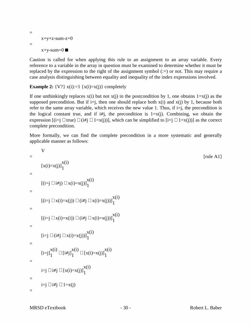
More formally, we can find the complete precondition in a more systematic and generallyapplicable manner as follows:

V= [rule A1]

[x(i)=x(j)]x(i)1

=

[(i=j ∨ i≠j) ∧ x(i)=x(j)]x(i)1

=

[(i=j ∧ x(i)=x(j)) ∨ (i≠j ∧ x(i)=x(j))]x(i)1

=

[(i=j ∧ x(i)=x(i)) ∨ (i≠j ∧ x(i)=x(j))]x(i)1

=

[i=j ∨ (i≠j ∧ x(i)=x(j))]x(i)1

=

[i=j]x(i)1 ∨ [i≠j]

x(i)1 ∧ [x(i)=x(j)]

x(i)1

=

i=j ∨ i≠j ∧ [x(i)=x(j)]x(i)1

=i=j ∨ i≠j ∧ 1=x(j)

=


i=j ∨ 1=x(j) ■Each reference in a postcondition to a variable of the array in question either (1) always refers tothe array variable to which assignment is being made, (2) never refers to the array variable towhich assignment is being made or (3) may or may not refer to the array variable to whichassignment is being made, depending upon the possible value(s) of the index expression inquestion. References of the third type must be eliminated by suitable algebraic manipulation, e.g.by a case distinction as in the above example, before replacing references to the variable inquestion by the expression on the right hand side of the assignment symbol (:=).

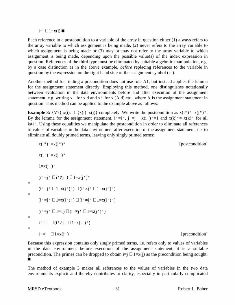
Another method for finding a precondition does not use rule A1, but instead applies the lemmafor the assignment statement directly. Employing this method, one distinguishes notationallybetween evaluation in the data environments before and after execution of the assignmentstatement, e.g. writing x' for x.d and x" for x.(A.d) etc., where A is the assignment statement inquestion. This method can be applied to the example above as follows:

Example 3: {V?} x(i):=1 {x(i)=x(j)} completely. We write the postcondition as x(i")"=x(j")".By the lemma for the assignment statement, i"=i', j"=j', x(i')"=1 and x(k)"= x(k)' for allk≠i'. Using these equalities we manipulate the postcondition in order to eliminate all referencesto values of variables in the data environment after execution of the assignment statement, i.e. toeliminate all doubly primed terms, leaving only singly primed terms:

x(i")"=x(j")" [postcondition]=

x(i')"=x(j')"=

1=x(j')"=

(i'=j' ∨ i'≠j') ∧ 1=x(j')"=

(i'=j' ∧ 1=x(j')") ∨ (i'≠j' ∧ 1=x(j')")=

(i'=j' ∧ 1=x(i')") ∨ (i'≠j' ∧ 1=x(j')")=

(i'=j' ∧ 1=1) ∨ (i'≠j' ∧ 1=x(j')')=

i'=j' ∨ (i'≠j' ∧ 1=x(j')')=

i'=j' ∨ 1=x(j')' [precondition]

Because this expression contains only singly primed terms, i.e. refers only to values of variablesin the data environment before execution of the assignment statement, it is a suitableprecondition. The primes can be dropped to obtain i=j ∨ 1=x(j) as the precondition being sought.■The method of example 3 makes all references to the values of variables in the two dataenvironments explicit and thereby contributes to clarity, especially in particularly complicated


expressions. On the other hand, it usually leads to lengthier and more tedious derivations.Generally, one should use the method of example 2 and revert to the method of example 3 onlywhen confusion arises.

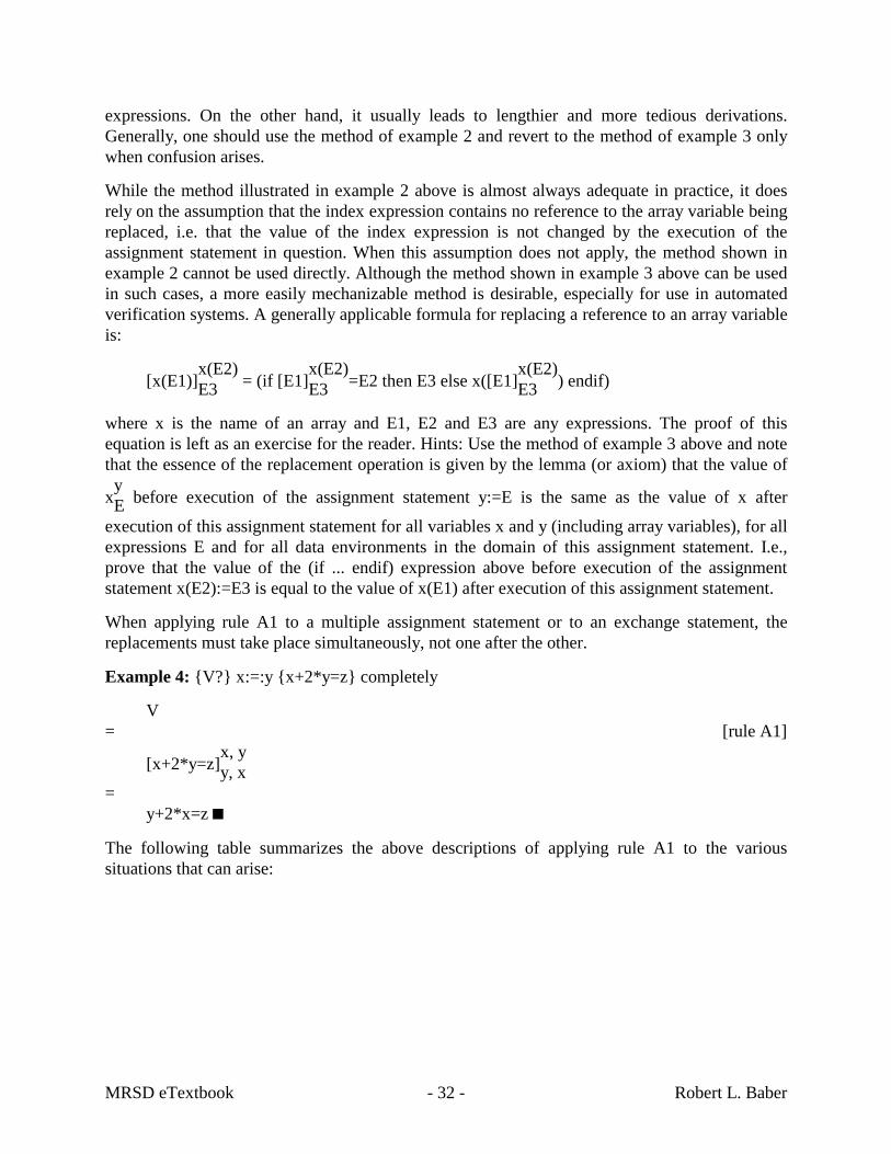
While the method illustrated in example 2 above is almost always adequate in practice, it doesrely on the assumption that the index expression contains no reference to the array variable beingreplaced, i.e. that the value of the index expression is not changed by the execution of theassignment statement in question. When this assumption does not apply, the method shown inexample 2 cannot be used directly. Although the method shown in example 3 above can be usedin such cases, a more easily mechanizable method is desirable, especially for use in automatedverification systems. A generally applicable formula for replacing a reference to an array variableis:

[x(E1)]x(E2)E3 = (if [E1]

x(E2)E3 =E2 then E3 else x([E1]

x(E2)E3 ) endif)

where x is the name of an array and E1, E2 and E3 are any expressions. The proof of thisequation is left as an exercise for the reader. Hints: Use the method of example 3 above and notethat the essence of the replacement operation is given by the lemma (or axiom) that the value of

xyE before execution of the assignment statement y:=E is the same as the value of x after

execution of this assignment statement for all variables x and y (including array variables), for allexpressions E and for all data environments in the domain of this assignment statement. I.e.,prove that the value of the (if ... endif) expression above before execution of the assignmentstatement x(E2):=E3 is equal to the value of x(E1) after execution of this assignment statement.

When applying rule A1 to a multiple assignment statement or to an exchange statement, thereplacements must take place simultaneously, not one after the other.

Example 4: {V?} x:=:y {x+2*y=z} completely

V= [rule A1]

[x+2*y=z]x, yy, x

=y+2*x=z ■

The following table summarizes the above descriptions of applying rule A1 to the varioussituations that can arise:


variable in thepostcondition

variable to theleft of :=

additionalcondition

example ofexpression

final result

simple simple differentvariables [x]

yE x

simple simple same variable[x]

xE (E)

simple array —[x]

y(E1)E2 x

array simple —[x(E1)]

yE2 x([E1]

yE2)

array array different arrays[x(E1)]

y(E2)E3 x([E1]

y(E2)E3 )

array array same array[x(E1)]

x(E2)E3 if [E1]

x(E2)E3 =E2

then (E3)

else x([E1]x(E2)E3 )

Results of applying rule A1 to the various types of variablesin the postcondition and to the left of the assignment symbol (:=)

4.4.2 Rule A2

If

V ⇒ PxE

then

{V} x:=E {P}

Proof:

{V} x:=E {P}⇐ [rule P1]

V ⇒ PxE ∧ {P

xE} x:=E {P}

= [rule A1]

V ⇒ PxE ■

Rule A2, which is simply a combination of rules P1 and A1, provides a way of verifying acorrectness proposition about an assignment statement. To verify that {V} x:=E {P}, one verifies


that V ⇒ PxE. Thus the task of verifying the correctness proposition {V} x:=E {P} is reduced to

the task of verifying the universal truth of a Boolean algebraic expression.

Example: {j≥0} k:=j+1 {k≥0} ?

{j≥0} k:=j+1 {k≥0}⇐ [rule A2]

j≥0 ⇒ [k≥0]kj+1

=j≥0 ⇒ j+1≥0

=true ■

4.5 Rules for sequences of statements

4.5.1 Rule S1 for the sequence of statements

If

{V} S1 {P1} and{P1} S2 {P}

then

{V} (S1, S2) {P}

Proof:

{V} (S1, S2) {P}= [lemma for an ordinary precondition]

V∩(S1, S2)-1.ID ⊆ (S1, S2)-1.P=

V∩S1-1.(S2-1.ID) ⊆ S1-1.(S2-1.P) (1)

But

{V} S1 {P1} ∧ {P1} S2 {P}= [lemma for an ordinary precondition]

[V∩S1-1.ID ⊆ S1-1.P1] ∧ [P1∩S2-1.ID ⊆ S2-1.P]⇒

[V∩S1-1.ID ⊆ S1-1.P1] ∧ [S1-1.(P1∩S2-1.ID) ⊆ S1-1.(S2-1.P)]=

[V∩S1-1.ID ⊆ S1-1.P1] ∧ [(S1-1.P1)∩S1-1.(S2-1.ID) ⊆ S1-1.(S2-1.P)]⇒

V∩(S1-1.ID)∩S1-1.(S2-1.ID) ⊆ S1-1.(S2-1.P)


= [S2-1.ID⊆ ID, S1-1.(S2-1.ID)⊆ S1-1.ID]V∩S1-1.(S2-1.ID) ⊆ S1-1.(S2-1.P) ■ [= (1) above]

Rule S1 may be extended in the obvious way for an arbitrarily long sequence of programstatements.

Strict and complete versions of rule S1 are also valid. The proof of the complete version is theabove proof of the ordinary version with the symbol ⊆ replaced by =. The strict version can beproved as follows:

Rule S1, strict version: If {V} S1 {P1} strictly and {P1} S2 {P} strictly, then {V} (S1, S2) {P}strictly.

Proof:

{V} S1 {P1} strictly and {P1} S2 {P} strictly= [lemma for a strict precondition]

V⊆ S1-1.P1 ∧ P1⊆ S2-1.P⇒

V⊆ S1-1.P1 ∧ S1-1.P1 ⊆ S1-1.(S2-1.P)⇒

V⊆ (S1, S2)-1.P= [lemma for a strict precondition]

{V} (S1, S2) {P} strictly ■Rule S1 has an important implication for practice: the postcondition may be transformed,working statement by statement from the end of a sequence of statements to the beginning, into aprecondition with respect to the entire sequence. If in every step a complete precondition isderived, then the final precondition is a complete precondition with respect to the entire sequenceof statements.

When applying rule S1 in order to verify a correctness proposition about a sequence of programstatements, intermediate conditions (P1 above) are required and, if not given, must be derived.Thus, the application of rule S1 to the task of verifying a correctness proposition gives rise to theneed for rules to derive preconditions for a given postcondition and a given statement.

4.5.2 Rule S2 for the sequence of assignment statements

Frequently a correctness proposition about a sequence of assignment statements must be proved.For such situations it is convenient to combine rules S1, A1 and A2 into rule S2:

If

V ⇒ [[ ... [PxnEn] ... ]

x2E2]

x1E1

then


{V}x1:=E1x2:=E2...xn:=En{P}

Note the sequence in which the several variable names are replaced by the correspondingexpressions: from the bottom to the top of the sequence of assignment statements. In effect, ruleA1 is applied to the last assignment statement first, then to the second last assignment statement,etc., and finally rule A2 is applied to the first assignment statement.

4.6 Rules for the if statement

Two rules for the if statement are formulated and proved below. One facilitates verifying acorrectness proposition, the other gives a rule for deriving a precondition for a givenpostcondition and a given if statement.

We begin by considering the preimage of P (a subset of ID) under the if statement


abbreviated S below. Furthermore, let Bt be the subset of ID upon which B is true (the preimageof true under B) and Bf be the subset of ID upon which B is false (the preimage of false under B).The preimage of P under S consists of those data environments which S maps into P. These arethe data environments (1) which are in Bt and which S1 maps into P, i.e. which are in Bt and inthe preimage of P under S1 or (2) which are in Bf and which S2 maps into P, i.e. which are in Bfand in the preimage of P under S2. (Cf. the domain of the if statement in section 2.5.6 above.)More formally,

S-1.P = (Bt∩S1-1.P ∪ Bf∩S2-1.P)

4.6.1 Rule IF1 for verifying a correctness proposition about an if statement

If

{V and B} S1 {P} and{V and not B} S2 {P}

then

{V} if B then S1 else S2 endif {P}

Proof:

{V and B} S1 {P} and {V and not B} S2 {P}= [lemma for an ordinary precondition]

(V∩Bt∩S1-1.ID ⊆ S1-1.P) ∧ (V∩Bf∩S2-1.ID ⊆ S2-1.P)=

(V∩Bt∩S1-1.ID ⊆ Bt∩S1-1.P) ∧ (V∩Bf∩S2-1.ID ⊆ Bf∩S2-1.P)


⇒(V∩Bt∩S1-1.ID ∪ V∩Bf∩S2-1.ID) ⊆ (Bt∩S1-1.P ∪ Bf∩S2-1.P)

=[V∩(Bt∩S1-1.ID ∪ Bf∩S2-1.ID)] ⊆ (Bt∩S1-1.P ∪ Bf∩S2-1.P)

=V∩S-1.ID ⊆ S-1.P

= [lemma for an ordinary precondition]{V} S {P} ■

Rule IF1 decomposes a correctness proposition to be verified into two correctness propositionsabout smaller program segments. Each must be verified by applying the rules appropriate for thestructures of the then and the else parts of the original if statement.

The complete version of rule IF1 holds. The strict version does not hold, because V need notimply that B is defined (true or false).

4.6.2 Rule IF2 for deriving a precondition with respect to an if statement

If

{V1} S1 {P} and{V2} S2 {P}

then

{V1 and B or V2 and not B} if B then S1 else S2 endif {P}

Proof:

{V1 and B or V2 and not B} if B then S1 else S2 endif {P}⇐ [rule IF1]

{[V1 and B or V2 and not B] and B} S1 {P}and {[V1 and B or V2 and not B] and not B} S2 {P}

={V1 and B} S1 {P} and {V2 and not B} S2 {P}

⇐ [rule P1]{V1} S1 {P} and {V2} S2 {P} ■

The complete version of rule IF2 holds. Provided that the condition (function) B is extended to IDin such a way that not B is true if and only if B is false, the strict version of rule IF2 also holds.

4.7 Rules for the while loop

In this section two rules for the while loop are formulated and proved. The first deals with awhile loop alone. Associated with almost every loop is an initialization, so a second rule for awhile loop together with its initialization will be formulated and proved. From a theoreticalstandpoint the second rule contains nothing new, but from a practical standpoint it is much moreimportant. The second rule provides more insight into the practical application of these concepts,especially in connection with designing a loop.


In proving the rules for the while loop, the following preliminary facts and lemmata will beneeded. The while statement while B do S endwhile is often abbreviated W below.

Preimage of a set under a while statement: In section 2.5.7 above the domain of a whilestatement was derived. In the same way one can derive the preimage of a subset P of ID under awhile statement. The result is:

W-1.P = ∪ ∞n=0 S-n.(P∩Bf) ∩

n-1j=0 S-j.Bt

Lemma 4.7 A: Given are the while statement while B do S endwhile and a subset I of ID. Thesubsets Bf and Bt of ID are defined to be the sets upon which the condition B is false and truerespectively. I.e. Bf = B-1.{false} and Bt = B-1.{true}. Then

I∩Bt∩S-1.ID ⊆ S-1.I⇒

I∩S-(n+1).Bf ∩nj=0 S-j.Bt ⊆ S-1.I ∩S-(n+1).Bf ∩

nj=0 S-j.Bt

for every non-negative integer n.

Proof:

I∩Bt∩S-1.ID ⊆ S-1.I⇒ [∩ same terms to both sides]

I∩Bt∩S-1.ID∩S-(n+1).Bf ∩nj=0 S-j.Bt ⊆ S-1.I ∩S-(n+1).Bf ∩

nj=0 S-j.Bt

⇒ [n≥0, Bt is the 0-th term in the ∩-series, S-n.Bf⊆ ID, S-(n+1).Bf = S-1.(S-n.Bf)⊆ S-1.ID]

I∩S-(n+1).Bf ∩nj=0 S-j.Bt ⊆ S-1.I ∩S-(n+1).Bf ∩

nj=0 S-j.Bt ■

The essence of the proof of the first rule below for the while loop lies in the following lemma.The condition I (a subset of ID) is called the loop invariant. This important condition will appearagain later.

Lemma 4.7 B: Given are the while statement while B do S endwhile and subsets I, Bf and Bt ofID as in lemma 4.7 A above. Then

I∩Bt∩S-1.ID ⊆ S-1.I⇒

I∩S-n.Bf ∩n-1j=0 S-j.Bt ⊆ S-n.(I∩Bf) ∩

n-1j=0 S-j.Bt

for every non-negative integer n.

Proof: This lemma will be proved by induction on n.


Proof of the base case: In the base case (n=0) the thesis of this lemma becomes

... ⇒ I∩Bf ⊆ I∩Bf

which is clearly true.

Inductive step: In the inductive step, the truth of the lemma for n will be assumed, i.e.

I∩Bt∩S-1.ID ⊆ S-1.I⇒ [inductive assumption]


n-1j=0 S-j.Bt

and the truth of the lemma for n+1 will be proved, i.e.

I∩Bt∩S-1.ID ⊆ S-1.I⇒ [to be proved]

I∩S-(n+1).Bf ∩nj=0 S-j.Bt ⊆ S-(n+1).(I∩Bf) ∩

nj=0 S-j.Bt

Proof of the inductive step:

I∩Bt∩S-1.ID ⊆ S-1.I⇒ [inductive assumption]


n-1j=0 S-j.Bt

⇒ [S-1 each side]

S-1.I∩S-(n+1).Bf ∩n-1j=0 S-(j+1).Bt ⊆ S-(n+1).(I∩Bf) ∩

n-1j=0 S-(j+1).Bt

⇒ [redefine running variables]

S-1.I∩S-(n+1).Bf ∩nj=1 S-j.Bt ⊆ S-(n+1).(I∩Bf) ∩

nj=1 S-j.Bt

⇒ [∩Bt to each side]

S-1.I∩S-(n+1).Bf ∩nj=0 S-j.Bt ⊆ S-(n+1).(I∩Bf) ∩

nj=0 S-j.Bt

⇒ [lemma 4.7 A, ⊆ transitive]

I∩S-(n+1).Bf ∩nj=0 S-j.Bt ⊆ S-(n+1).(I∩Bf) ∩

nj=0 S-j.Bt ■

4.7.1 Rule W1 for the while loop without initialization

If

{I and B} S {I}


then

{I} while B do S endwhile {I and not B}

Note: In the proof below, the entire while statement (while B do S endwhile) is abbreviated W.

Proof:

{I and B} S {I}= [lemma for an ordinary precondition]

I∩Bt∩S-1.ID ⊆ S-1.I⇒ [lemma 4.7 B]

and∞n=0 [I∩S-n.Bf ∩

n-1j=0 S-j.Bt ⊆ S-n.(I∩Bf) ∩

n-1j=0 S-j.Bt]

⇒

∪ ∞n=0 I∩S-n.Bf ∩

n-1j=0 S-j.Bt ⊆ ∪ ∞

n=0 S-n.(I∩Bf) ∩n-1j=0 S-j.Bt

=

I∩(∪ ∞n=0 S-n.Bf ∩

n-1j=0 S-j.Bt) ⊆ ∪ ∞

n=0 S-n.(I∩Bf) ∩n-1j=0 S-j.Bt

=I∩W-1.ID ⊆ W-1.( I∩Bf)

= [lemma for an ordinary precondition]{I} while B do S endwhile {I and not B} ■

4.7.2 Rule W2 for the while loop with initialization

If

{V} init {I} and [start]{I and B} S {I} and [during execution]I and not B ⇒ P [end]

then

{V} init; while B do S endwhile {P}

Proof:

{V} init; while B do S endwhile {P}⇐ [rule S1]

[{V} init {I}] and [{I} while B do S endwhile {P}]⇐ [rule P1]

[{V} init {I}] and [{I} while B do S endwhile {I and not B}] and [I and not B ⇒ P]⇐ [rule W1]

[{V} init {I}] and [{I and B} S {I}] and [I and not B ⇒ P] ■


The condition V above is in general an ordinary precondition. It does not guarantee that the whileloop will execute to yield a defined result, in particular, that the recursive definition of the whileloop will terminate (equivalently, that the execution of the loop will terminate).

The condition I is true before execution of the loop begins, before and after each execution of theloop body S and after the execution of the loop has terminated. The condition I is therefore calledthe loop invariant. The loop invariant is the most important concept in designing a loop, inunderstanding a loop and in proving a loop to be correct. It expresses the main design decision inthe construction of a loop.

In order to prove a correctness proposition about a loop, one must

1. identify a suitable loop invariant I if not already given by the software designer,2. prove that the initialization establishes the initial truth of the loop invariant I,3. prove that the execution of the loop body S preserves the truth of the loop invariant I,4. prove that the truth of the loop invariant I and the falsehood of the loop condition B

together imply the truth of the postcondition and5. prove that the loop will be executed with a defined result, in particular, that the loop

terminates.

Steps 1 through 4 ensure partial correctness of the loop. Step 5 in addition ensures totalcorrectness.

For every loop a loop invariant!

In order to design a loop, the software developer must

1. decide upon a suitable loop invariant I,2. design the initialization so that it establishes the initial truth of the loop invariant I,

{V} init? {I}3. design the while condition B so that

I and not B? ⇒ Pand

4. design the body S of the loop so that it preserves the truth of the loop invariant I{I and B} S? {I}while ensuring progress toward (not B) or P, in order to ensure that the loop willterminate.

For every loop a loop invariant!

The first step in designing a loop must be to decide upon a loop invariant, because every otherstep requires it. Step 2 can be performed independently of steps 3 and 4. The result of step 3 (thewhile condition B) is a prerequisite for step 4.

Note that the loop invariant I is true (usually in a trivial way) before execution of the loop begins.When execution terminates, it is also true (I and not B is true). In other words, the initial andfinal situations are special cases of the loop invariant I. Viewed the other way around, the loopinvariant is a generalization of the initial and final states. Roughly speaking, the loop invariant Ican be thought of as a generalization of the precondition V and the postcondition P (even though


this statement is not mathematically correct). This observation gives us a useful guideline fordesigning a loop invariant. A number of rules of thumb have been formulated for deciding upon aloop invariant; all are variations of the idea of generalizing the initial and final conditions.Section 8.4 below contains additional guidelines on formulating suitable loop invariants.

The requirement [I and not B ⇒ P] can be written in many equivalent ways, some of whichsuggest useful approaches for deriving B. The most useful forms are probably:

1. I and not B ⇒ P2. I and not P ⇒ B3. I ⇒ (not B ⇒ P)4. I ⇒ (not P ⇒ B)

These forms suggest the following questions and strategies for determining a suitable whilecondition B:

1. What condition in addition to I ensures the truth of P? (The answer is the negation of B.)

2a. What must be true if I is true, but P is not? Use this condition as B.

2b. Form the expression for [I and not P] and simplify and weaken it to obtain B.

3. Simplify and strengthen P, assuming the truth of I, to obtain an expression for not B. Negatethe result to obtain B.

4. Simplify and weaken the negation of P, assuming the truth of I, to obtain B.

In each case, B must be in a form which is syntactically permitted as a while condition. Note that(not P) is always semantically a correct candidate for B, but is seldom permitted syntactically.The goal of the algebraic manipulations outlined above is to transform the expression in questioninto a form which is syntactically allowed as a while condition in the target programminglanguage(s).

4.7.3 Loop termination

A common and practical way to prove that a loop terminates uses the concept of a loop variant.A loop variant is an expression whose value• is decreased (or increased) by at least a fixed amount (e.g. 1) by each execution of the body of

the loop and• has a lower (or upper) bound.

The loop variant’s bound derives from either the loop invariant or the loop condition, often both.

Example: Consider the loop

while i<n do i:=i+1; S1 endwhile

where the program segment S1 does not modify the value of i. Typically, the loop invariant forsuch a loop would contain the term i≤n. A suitable loop variant for this loop would be (n-i). Eachexecution of the body of the loop decreases the value of this expression by one. The loop condi-


tion guarantees that every time execution of the body of the loop begins, 0<n-i, so 0 is a lowerbound for the loop variant. Also, the loop invariant ensures that 0≤n-i, i.e. that 0 is a lower boundfor the loop variant. Thus the loop cannot continue to execute indefinitely.

Note that mathematical convergence to the lower (or upper) bound is not sufficient. The boundmust be potentially violated in order to prove termination. When the loop variable is not neces-sarily an integer, this can give rise to situations which must be very carefully analyzed, bothwhen designing loops and when proving that they terminate. Rounding when calculating the nextvalue of a floating point loop variable can complicate the analysis further. In practice such situa-tions arise in which it is “intuitively clear” that a loop must terminate, but it does not, in fact,always do so. Several simple and obvious algorithms for finding the zero of a function are exam-ples of this problem, including (1) a binary search with too small an error tolerance and (2) linearinterpolation.

The informally stated requirements above are sufficient for manually verifying termination inmany practical cases. When a more formal approach is desired, the following lemma is useful.

Lemma for loop termination: Let the loop

while B do S endwhile

and a suitable loop invariant I (see rules W1 and W2 above) be given. If a numerical function varand a positive constant ε exist such that

I ⇒ (B ⇒ 0<var) and [alternatively: I ⇒ (var≤0 ⇒ not B), see below]{I and B and var = var'} S {var ≤ var'-ε}

then the above while loop will terminate (i.e. S will not be executed indefinitely). ■The condition (B ⇒ 0<var) often provides a convenient way to determine a suitable loop variantfunction var. Manipulate and weaken appropriately the expression for the while condition B intothe form 0<..., and the expression to the right of the < symbol is a candidate for the loop variantvar. While simplifying and weakening B, one may assume that the loop invariant I is true (issatisfied).

Note that

B ⇒ 0<var

is logically equivalent to

var≤0 ⇒ not B

so that the first condition in the lemma above can be written in the alternative form

I ⇒ (var≤0 ⇒ not B)

When this condition is written in this form, the validity of the lemma is perhaps more obvious:Because each execution of S reduces the value of var by at least the fixed amount ε, after var'/εexecutions of S the value of var will be zero or less, so B will be false and the loop will termi-


nate. I.e., var'/ε is an upper bound on the number of times S will execute, a fact that is sometimeshelpful when analyzing the time complexity of such a loop.

The sketch in the preceding paragraph of the proof of the lemma highlights the fact that there isnothing special about the value 0 for the lower bound of the loop variant. All that is necessary toensure termination is that the while condition B (together with the loop invariant if needed)implies the existence of some lower bound for the loop variant.

Often, ε is the constant 1 and the condition (B = (0<var)) – which is stronger than the first condi-tion in the lemma above – can be easily fulfilled by choosing var suitably. Loops that sequentiallyprocess all elements of a one dimensional array are typical examples of such cases. Notice that inthe previous example above, B is i<n, which is equivalent to 0<n-i, so the obvious choice for theloop variant function var is (n-i).

The equality in the condition (B = (0<var)) above is too strong for some applications. If theexample referred to above were searching for an array element with a certain value, the whilecondition B might be i<n and Z(i)≠key (instead of just i<n). The same loop variant function (n-i)applies and enables one to easily show that the loop must terminate, regardless of whether or notan array element with the value key is present. Here, B does imply that var is positive, but thereverse is not true, so B is not equivalent to the condition that var is positive.

As an example of a situation requiring the still weaker form of the first condition in the lemmaabove, i.e. I ⇒ (B ⇒ 0<var), consider a loop for processing every element of a two dimensionalarray X(j, k) with index j between 1 to Nj inclusive and index k between 1 to Nk inclusive. If theloop invariant I contains the terms 1≤Nj and 1≤Nk and j≤Nj and k≤Nk and if the while conditionB is (j<Nj or k<Nk), then one suitable loop variant function var is Nj*(Nk-k) + (Nj-j). B alonedoes not imply that var is positive; also I is needed in order to show that var is positive.

A rule for a strict precondition for a while loop is presented in section 7.7 below. That rule in-cludes the above lemma for loop termination.

4.8 Rules for the subprogram

The following rules are basically notational variants of previous rules. They have been put into aform here which is particularly suited for applying to subprograms and subprogram calls. Theycan also be applied to any program segment.

4.8.1 Rule SP1

If the execution of the program segment S does not modify any variable appearing in thecondition B, then B has the same value before and after the execution of S. B is therefore aprecondition of itself with respect to S:

{B} S {B}

4.8.2 Rule SP2

If

{B} S {B} and


{V} S {P}

then

{B and V} S {B and P}

Rule SP2 follows from rules SP1 and DC1.

To apply rule SP2, separate the postcondition into two anded parts. One part should referenceonly variables not changed by the execution of S; this part is its own precondition and is thecondition B of this rule. The second part of the postcondition contains all references to variableswhich may be changed by the execution of S; this part is P. The precondition is separated intocorresponding parts B and V.

4.8.3 Rule SP3

If

{B} S {B} andV ⇒ V1{V1} S {P1}P1 ⇒ P

then

{B and V} S {B and P}

Rule SP3 combines rules SP2 and P1.

Typically, {V1} S {P1} is the given specification of S. B is a condition established by theprogram before S that is not affected by the execution of S. This rule takes into account the factsthat (1) the previous program may establish a condition stronger than that required by S and (2) Smay establish a stronger condition (P1) than that actually required by the subsequent program(P).

4.9 Rules for the declare statement

4.9.1 Applying rules for the assignment statement to the declare statement

The declare statement has the same effect upon the values of program variables as thecorresponding assignment statement. In particular, the lemma for the assignment statement alsoholds for the declare statement, provided that the postcondition does not refer to the setassociated with the variable being declared (because that set may be changed by the execution ofthe declare statement). Because the proof of rule A1 depends only upon that lemma (and notupon other aspects of the definition of the assignment statement), rule A1 applies also to thedeclare statement

{PxE} declare (x, S, E) {P} completely


provided that P contains no reference to Set.”x”. Rule A2, being nothing other than acombination of rules A1 and P1, also applies in this case to the declare statement:

[V ⇒ PxE] ⇒ [{V} declare (x, S, E) {P}]

To derive a precondition or to verify a correctness proposition about a declare statement whenthe postcondition refers to the set associated with the variable being declared, one may use thefollowing more general rules D1 and D2, which are corresponding extensions of the rules A1 andA2 above.

4.9.2 Rule D1

Let the condition P and the statement declare (x, S, E) be given. If one forms the condition V byreplacing in P• every reference to the value of the variable x by the expression E (in parentheses) and,

simultaneously,• every reference to the set associated with the variable x by S,then V is a complete precondition of P with respect to the declare statement, i.e.

{Px,E,

Set.“x”S } declare (x, S, E) {P} completely

Proof: The proof of this rule is very similar to the proof of rule A1. ■This rule is due to Amitha Perera [personal communication].

Note the similarity between rules A1 and D1. In rule A1 for an assignment statement, onlyreferences to the value of the variable x are replaced, because the assignment statement changesonly the value of the variable x. In rule D1 for the declare statement, both references to the valueof the variable x and references to the set associated with the variable x are replaced, because thedeclare statement changes both the value of the variable x and the set associated with the variablex.

If P contains no reference to the set associated with the variable x (e.g. Set.“x”), rules A1 and D1give the same precondition.

4.9.3 Rule D2

If

V ⇒ Px,E,

Set.“x”S

then

{V} declare (x, S, E) {P}

Proof: See the proof of rule A2 above. ■


Rule D2, which is simply a combination of rules P1 and D1, provides a way of verifying acorrectness proposition about a declare statement. To verify that {V} declare (x, S, E) {P}, one

verifies that V ⇒ Px,E,

Set.“x”S . Thus the task of verifying the correctness proposition about a

declare statement is reduced to the task of verifying the universal truth of a Boolean algebraicexpression.

Note the correspondence between the pair of rules A1 and A2 and the pair of rules D1 and D2.

4.10 Applying rules to other types of program statements

4.10.1 Rules applicable to the release statement

In proofs of correctness, two different aspects concerning a release statement typically arise.

First, one must usually show that a certain structure of the data environment (often the samestructure as a previous data environment) is established after the release statement has beenexecuted. Typically this can be done by applying the definition of the release statement directly.

Second, one must show that a certain postcondition holds after execution of the releasestatement. Because the variable being released no longer exists after execution of the releasestatement, the postcondition will not refer to that variable. Often it will not refer to any othervariable of the same name. The postcondition is then an expression whose value is not changedby the execution of the release statement and rule SP1 above applies:

{B} release x {B}, if the value of B is not affected by the execution of release x.

If the postcondition of a release statement does refer to a variable of the same name as thevariable being released, the variable being so referenced is not the variable being released, but thenext variable of the same name in the data environment before executing the release statement. Insuch a case it is usually convenient to consider the program segment ending with the releasestatement in question and beginning with the previous declare statement that declared thatvariable:

{V}declare (x, ., .)...release x{P}

One then notes that this program segment does not change the value of a program variable namedx, if any exists in the data environment before execution of the declare statement. That part of thepostcondition P referring to such a variable x should be separated from those parts referring tovariables modified by the program segment and then either rule SP2 or SP3 applied.

The procedures outlined above are usually adequate when manually verifying the correctness of aprogram. Generally valid formal rules for declare and release statements, suitable also formechanized verification, are given in Chapter 9 below.


4.10.2 The null statement

The null statement changes nothing in the data environment (null.d=d, for all d∈ ID), therefore,the value of any condition remains unchanged by its execution. Therefore, {B} null {B}, for anycondition B.


5. Applying the rules in proofs of correctness: examples

To verify a correctness proposition about a program segment, one applies the relevant rulesiteratively in order to decompose the correctness proposition to be proved into correctnesspropositions about ever smaller program segments until the level of basic statements (theassignment, declare, release and null statements) is reached. The remaining correctnesspropositions about such statements are then proved either by applying the applicable rules andverifying the resulting Boolean algebraic expressions (implications) or by direct application ofthe definition of the statement in question.

At each step of this decomposition process, the particular program segment in question and theproof task (verifying a correctness proposition or deriving a precondition) together determine therule for decomposing the correctness proposition.

The following examples illustrate this process.

5.1 Proof of correctness of the linear search

In this example, the array A(i), i=1, ... n, is searched for the value of the variable x. The firstelement in A equal to x is to be found and its location (the value of its index in A) recorded andmade available to the succeeding or calling program.

Formally, we describe this program segment by its specified precondition V and postcondition P:

V: n∈ Z and 0≤n [empty array allowed]

P: n∈ Z and k∈ Z and 1≤k≤n+1 and found∈ IB [ranges of values of variables]

andk-1i=1 A(i)≠x [all A(i) before the kth ≠x]

and (k≤n and A(k)=x and found [x found]or k=n+1 and not found) [x not present in A]

The correctness proposition to be verified (theorem to be proved) is:

{V}k:=1 [initialization]while k≤n and A(k)≠x do

k:=k+1 Wendwhile found:=(k≤n)

{P}

The designer of this program segment specified the following loop invariant

I: n∈ Z and k∈ Z and 1≤k≤n+1 andk-1i=1 A(i)≠x

Proof: The correctness proposition above will be true by rule S1 if both of the following are true,where P1 is a condition yet to be determined:


{V} k:=1; W {P1} [1]

{P1} found:=(k≤n) {P} [2]

• Remaining to be proved are: [1], [2]

[2] will be true by rule A1 if P1=Pfoundk≤n , which is, after simplification, as follows:

P1: n∈ Z and k∈ Z and 1≤k≤n+1 [definition of P1]

andk-1i=1 A(i)≠x

and (k≤n and A(k)=x or k=n+1)

• Remaining to be proved is: [1]

[1] will be true by rule W2 if the following three conditions are true:

{V} k:=1 {I} [3]{I and k≤n and A(k)≠x} k:=k+1 {I} [4]I and not (k≤n and A(k)≠x) ⇒ P1 [5]

• Remaining to be proved are: [3], [4], [5]

[3] will be true by rule A2 if

V ⇒ Ik1 [6]

• Remaining to be proved are: [4], [5], [6]

[4] will be true by rule A2 if

I and k≤n and A(k)≠x ⇒ Ikk+1 [7]

• Remaining to be proved are: [5], [6], [7]. These propositions are all Boolean algebraicexpressions whose universal truth must be verified.

Proof of [6], which is: V ⇒ Ik1

Ik1

=n∈ Z and 1≤n+1

=n∈ Z and 0≤n

=V ■


• Remaining to be proved are: [5], [7]

Proof of [5], which is: I and not (k≤n and A(k)≠x) ⇒ P1

I and not (k≤n and A(k)≠x)=

I and (k>n or A(k)=x)=

I and (k>n or k≤n and A(k)=x)=

n∈ Z and k∈ Z and 1≤k≤n+1

andk-1i=1 A(i)≠x

and (k≤n and A(k)=x or k>n)=

n∈ Z and k∈ Z and 1≤k≤n+1

andk-1i=1 A(i)≠x

and (k≤n and A(k)=x or k=n+1)=

P1 ■• Remaining to be proved is: [7]

Proof of [7], which is: I and k≤n and A(k)≠x ⇒ Ikk+1

Ikk+1

=

n∈ Z and k+1∈ Z and 1≤k+1≤n+1 andk+1-1i=1 A(i)≠x

=

n∈ Z and k∈ Z and 0≤k≤n andki=1 A(i)≠x [7.1]

Furthermore,

I and k≤n and A(k)≠x=

n∈ Z and k∈ Z and 1≤k≤n+1 andk-1i=1 A(i)≠x and k≤n and A(k)≠x

= [note that the and series below is not empty]

n∈ Z and k∈ Z and 1≤k≤n andki=1 A(i)≠x

⇒


n∈ Z and k∈ Z and 0≤k≤n andki=1 A(i)≠x [7.1]

= [see above]

Ikk+1 ■

As an informal proof of termination of the loop, we note that each execution of the body of theloop increases the value of k by one. But both the while condition and the loop invariant containupper bounds on k, which the proof above shows will not be violated. Therefore, the body of theloop can be executed only a limited number of times.

This completes the verification of the correctness proposition about the linear search program.Note how the rules have been used to decompose the original correctness proposition to beproved in a hierarchical manner corresponding to the structure of the program. Thedecomposition process was repeated iteratively until only Boolean algebraic expressionsremained, which were then verified by algebraic manipulation. This is a typical structure forproofs of correctness of programs.

In addition, the following theorem about the behaviour of this program segment is of interest, e.g.when applying rules SP1, SP2 or SP3 to a call to this subprogram: The execution of the programsegment above changes at most the values of the program variables k and found; i.e., no othervariable is modified. The validity of this theorem is evident by inspection of the programsegment together with the definitions of the various types of statements appearing therein.

5.2 Strengthening the postcondition of the body of a loop

In the above example, part of the loop invariant I was the term 1≤k≤n+1 which bounds the loopvariable k above and below. Being part of the loop invariant, this term appeared in both theprecondition and the postcondition of the loop body:

{... 1≤k≤n+1 ...}k:=k+1{... 1≤k≤n+1 ...}

This correctness proposition will be true by rule A2 if

... 1≤k≤n+1 ... ⇒ [... 1≤k≤n+1 ...]kk+1

which is equivalent to

... 1≤k≤n+1 ... ⇒ [... 0≤k≤n ...]

Note that the lower and upper bounds have been shifted by the amount by which the loopvariable k was incremented or decremented. One new bound (here 0≤k) is automaticallysatisfied; the required precondition is weaker than the one actually satisfied. When workingbackward through the program segment, one can strengthen this condition (cf. rule P1). Carryingout this strengthening already in the postcondition of the loop body often simplifies the algebraicmanipulation of intermediate conditions prevailing at points within the body of the loop, e.g. by


ensuring that certain series are not empty. The other bound (here k≤n) is not automaticallysatisfied; some other term in the precondition must ensure that it is satisfied. This term typicallycomes from the loop condition, as it does in the example above.

Strengthening the postcondition in the above example would be done by requiring the followingstronger correctness proposition to be satisfied:

{... 1≤k≤n+1 ...}k:=k+1{... 2≤k≤n+1 ...}

If this correctness proposition is satisfied, the weaker one above will be satisfied by rule P1.

If, as in the example above, the execution of the body of the loop increases the value of the loopvariable, its lower bound in the postcondition may be increased correspondingly. If the executionof the body of the loop decreases the value of the loop variable, its upper bound in thepostcontion may be decreased correspondingly.

Whenever the execution of the loop body increases or decreases the value of the loop variable,one should consider strengthening the postcondition of the body of the loop as illustrated above.Doing so will sometimes simplify algebraic manipulation later in the proof and is, therefore,generally to be recommended.

5.3 Proof of correctness of the merge

5.3.1 External view of the subprogram merge

In this example, the values in two arrays A and B are merged and copied to the array C. Thevalues in the arrays A and B are assumed to be sorted before this subprogram is executed. Afterexecution of the subprogram merge the values in C must be sorted.

Formally, we describe this program segment by its specified (ordinary) precondition V andpostcondition P:

V: na∈ Z and 0≤na and nb∈ Z and 0≤nb [empty input arrays allowed]

andna-1i=1 A(i)≤A(i+1) and

nb-1i=1 B(i)≤B(i+1) [A, B sorted]

P: (&na+nbi=1 [C(i)]) Perm (&

nai=1 [A(i)] &

nbi=1 [B(i)]) [final values in C

come from A and B]

andna+nb-1i=1 C(i) ≤C(i+1) [C sorted]

The function Perm (permutation) above, written as an infix operator, maps a pair of sequences tothe set {false, true}. Perm is defined axiomatically as follows:

[] Perm [] [the empty sequence is a permutation of itself]

[(a & b & c) Perm (d & b & e)] = [(a & c) Perm (d & e)] [subsequences cancel]


where a, b, c, d and e are sequences.

Correctness proposition 1: {V} call merge {P}

Correctness proposition 2: For every data environment d in the domain of the subprogrammerge, merge.d = d structurally.

Correctness proposition 3: The execution of the subprogram merge modifies at most the valuesof the variables C(i) for i∈ Z and 1≤i≤na+nb.

Correctness proposition 4: The execution of merge does not continue unendlessly, i.e.terminates in finite time.

5.3.2 Internal view of the subprogram merge

Correctness proposition 1:

{V}declare (ia, Z, 1); declare (ib, Z, 1); declare (ic, Z, 1) [abbreviated init below]while ia ≤ na or ib ≤ nb do [B1]

if ib > nb or (ia ≤ na and A(ia) ≤ B(ib)) W [B2]then C(ic) := A(ia); ia := ia + 1 S [S1]else C(ic) := B(ib); ib := ib + 1 [S2]endif ic := ic + 1

endwhile release ia; release ib; release ic [R]{P}

Correctness proposition 2: For all d in the domain of the subprogram merge, merge.d = dstructurally. This theorem can be easily verified informally by inspection of the programsegment, see the definitions of the several types of program statements involved. ■Correctness proposition 3: The execution of the subprogram merge modifies at most the valuesof the variables C(i) for i∈ Z and 1≤i≤na+nb. With the exception of the range of i, this theoremcan also be easily verified informally by inspection. The stated bounds for the values of theindices to the array C will follow from the preconditions of the assignment statements C(ic):=...,see the proof below.

The designer of this program segment specified the following loop invariant

I: I0 and I1 and I2 and I3 and I4 and I5 and I6 and I7 and I8

where

I0: na∈ Z and 0≤na and nb∈ Z and 0≤nb [range of na, nb (from precondition)]I1: ia∈ Z and 1≤ia≤na+1 [range of ia]I2: ib∈ Z and 1≤ib≤nb+1 [range of ib]I3: (ic-1) = (ia-1) + (ib-1) [# in C = # from A + # from B]


I4: (&ic-1i=1 [C(i)]) Perm (&

ia-1i=1 [A(i)] &

ib-1i=1 [B(i)]) [values in C from A, B]

I5: (1<ic and ia≤na) ⇒ C(ic-1)≤A(ia) [next from A≥last into C, if any]I6: (1<ic and ib≤nb) ⇒ C(ic-1)≤B(ib) [next from B≥last into C, if any]

I7: andic-2i=1 C(i)≤C(i+1) [C sorted]

I8: andna-1i=1 A(i)≤A(i+1) and

nb-1i=1 B(i)≤B(i+1) [A, B sorted]

Note that this loop invariant is symmetrical in a and b, i.e. if one replaces ia, ib, na, nb, A and Bsimultaneously by ib, ia, nb, na, B and A respectively, then the result is the loop invariant itself.We will make use of this symmetry in the proof below in order to reduce the amount of algebraicmanipulation required to complete the proof.

Proof of correctness proposition 1: Correctness proposition 1 will be true by rule S1 if both of thefollowing are true:

{V} init, W {P} [1]{P} R {P} [2]

• Remaining to be proved are: [1], [2].

[2] is true by rule SP1 because P contains no references to ia, ib or ic, the variables beingreleased by the statements in R.

• Remaining to be proved is: [1].

[1] will be true by rule W2 if all of the following are true:

{V} init {I} [3]{I and B1} S, ic:=ic+1 {I} [4]I and not B1 ⇒ P [5*]

• Remaining to be proved are: [3], [4], [5*]. An asterisk (*) indicates that the proposition is aBoolean algebraic expression to be verified, which therefore does not need to be decomposedfurther by the application of rules.

[3] will be true by rules A1, A2 and S1 if

V ⇒ [[Iic1 ]

ib1 ]

ia1 [6*]

• Remaining to be proved are: [4], [5*], [6*].

[4] will be true by rules A1 and S1 if

{I and B1} S {Iicic+1} [7]

• Remaining to be proved are: [5*], [6*], [7].


[7] (in which S is an if statement) will be true by rule IF1 if

{I and B1 and B2} S1 {Iicic+1} [8]

{I and B1 and not B2} S2 {Iicic+1} [9]

• Remaining to be proved are: [5*], [6*], [8], [9]. Propositions 8 and 9 are nearly symmetrical;the following steps will transform one of them so that the resulting two propositions aresymmetrical, in which case only one needs to be algebraically verified.

We note that

B1 and B2= [ia≤na and [ib>nb or A(ia)≤B(ib)]]

and that

B1 and not B2= [ib≤nb and [ia>na or B(ib)<A(ia)]]

so that [8] and [9] can be rewritten as

{I and ia≤na and [ib>nb or A(ia)≤B(ib)]}

C(ic):=A(ia); ia:=ia+1 {Iicic+1} [8]

{I and ib≤nb and [ia>na or B(ib)<A(ia)]}

C(ic):=B(ib); ib:=ib+1 {Iicic+1} [9]

[9] will be true by rule P1 if the following correctness proposition with a weaker precondition istrue:

{I and ib≤nb and [ia>na or B(ib)≤A(ia)]}

C(ic):=B(ib); ib:=ib+1 {Iicic+1} [10]

• Remaining to be proved are: [5*], [6*], [8], [10].

Propositions 8 and 10 are symmetrical in a and b, i.e. if in either one ia, ib, na, nb, A and B aresimultaneously replaced by ib, ia, nb, na, B and A respectively, then the other proposition results.Therefore, a proof of either proposition can be transformed into a proof of the other by the samereplacement of the symbols occurring therein. Consequently, we need not prove both [8] and [10]algebraically; a proof of either suffices.

• Remaining to be proved are: [5*], [6*], [10].

[10] will be true by rules A1, A2 and S1 if


I and ib≤nb and [ia>na or B(ib)≤A(ia)] ⇒ [[Iicic+1]

ibib+1]

C(ic)B(ib) [11*]

• Remaining to be proved are: [5*], [6*], [11*]. I.e., only Boolean algebraic expressions muststill be verified. The right hand side of the implication [11*] would be long if written outcompletely. We therefore reduce this proposition further as follows.

[11*] will be true by a property of the implication ([(X⇒ Y) and (X⇒ Z)] = [X⇒ (Y and Z)]) (cf.rule DC3) if

I and ib≤nb and [ia>na or B(ib)≤A(ia)] ⇒ [[I0icic+1]

ibib+1]

C(ic)B(ib) [12*]


ibib+1]

C(ic)B(ib) [13*]


ibib+1]

C(ic)B(ib) [14*]


ibib+1]

C(ic)B(ib) [15*]


ibib+1]

C(ic)B(ib) [16*]


ibib+1]

C(ic)B(ib) [17*]


ibib+1]

C(ic)B(ib) [18*]


ibib+1]

C(ic)B(ib) [19*]


ibib+1]

C(ic)B(ib) [20*]

• Remaining to be proved are: [5*], [6*], [12*], [13*], [14*], [15*], [16*], [17*], [18*], [19*],[20*].

[5*] is true:

P=

(&na+nbi=1 [C(i)]) Perm (&

nai=1 [A(i)] &

nbi=1 [B(i)])

andna+nb-1i=1 C(i) ≤C(i+1)

⇐I4 and ic-1=na+nb and ia-1=na and ib-1=nb and I7 and ic-2=na+nb-1

⇐I4 and I7 and (ic-1)=(ia-1)+(ib-1) and ia=na+1 and ib=nb+1

⇐I3 and I4 and I7and na∈ Z and nb∈ Z and ia∈ Z and ia≤na+1 and ib∈ Z and ib≤nb+1


and ia>na and ib>nb⇐

I0 and I1 and I2 and I3 and I4 and I7 and ia>na and ib>nb⇐

I and ia>na and ib>nb=

I and not B1 ■• Remaining to be proved are: [6*], [12*], [13*], [14*], [15*], [16*], [17*], [18*], [19*], [20*].

[6*] is true:

[[Iic1 ]

ib1 ]

ia1

=na∈ Z and 0≤na and nb∈ Z and 0≤nb

andna-1i=1 A(i)≤A(i+1) and

nb-1i=1 B(i)≤B(i+1)

=V ■

• Remaining to be proved are: [12*], [13*], [14*], [15*], [16*], [17*], [18*], [19*], [20*].

[12*] is true:

[[I0icic+1]

ibib+1]

C(ic)B(ib)

= [I0 contains no references to ic, ib or C(.)]I0

⇐I

⇐I and ib≤nb and [ia>na or B(ib)≤A(ia)] ■

• Remaining to be proved are: [13*], [14*], [15*], [16*], [17*], [18*], [19*], [20*].

[20*] is true:

[[I8icic+1]

ibib+1]

C(ic)B(ib)


⇐I


• Remaining to be proved are: [13*], [14*], [15*], [16*], [17*], [18*], [19*].


[13*] is true:

[[I1icic+1]

ibib+1]

C(ic)B(ib)


⇐I


• Remaining to be proved are: [14*], [15*], [16*], [17*], [18*], [19*].

[14*] is true:

[[I2icic+1]

ibib+1]

C(ic)B(ib)

=ib+1∈ Z and 1≤ib+1≤nb+1

=ib∈ Z and 0≤ib≤nb

⇐ib∈ Z and 1≤ib≤nb+1 and ib≤nb

=I2 and ib≤nb


• Remaining to be proved are: [15*], [16*], [17*], [18*], [19*].

[15*] is true:

[[I3icic+1]

ibib+1]

C(ic)B(ib)

=(ic+1-1) = (ia-1) + (ib+1-1)

=(ic-1) = (ia-1) + (ib-1)

=I3


• Remaining to be proved are: [16*], [17*], [18*], [19*].

[16*] is true:


[[I4icic+1]

ibib+1]

C(ic)B(ib)

=

[(&ici=1 [C(i)]) Perm (&

ia-1i=1 [A(i)] &

ibi=1 [B(i)])]

C(ic)B(ib)

⇐

1≤ib and 1≤ic and [(&ici=1 [C(i)]) Perm (&

ia-1i=1 [A(i)] &

ibi=1 [B(i)])]

C(ic)B(ib)

=

[1≤ib and 1≤ic and (&ici=1 [C(i)]) Perm (&

ia-1i=1 [A(i)] &

ibi=1 [B(i)])]

C(ic)B(ib)

=[1≤ib and 1≤ic

and (&ic-1i=1 [C(i)] & [C(ic)])

Perm (&ia-1i=1 [A(i)] &

ib-1i=1 [B(i)] & [B(ib)])]

C(ic)B(ib)

=[1≤ib and 1≤ic

and (&ic-1i=1 [C(i)] & [B(ib)]) Perm (&

ia-1i=1 [A(i)] &

ib-1i=1 [B(i)] & [B(ib)])

=

[1≤ib and 1≤ic and (&ic-1i=1 [C(i)]) Perm (&

ia-1i=1 [A(i)] &

ib-1i=1 [B(i)])

=I4 and 1≤ib and 1≤ic

⇐I4 and 1≤ia and 1≤ib and (ic-1) = (ia-1) + (ib-1)

⇐I1 and I2 and I3 and I4


• Remaining to be proved are: [17*], [18*], [19*].

[19*] is true:

[[I7icic+1]

ibib+1]

C(ic)B(ib)

=

[[[andic-2i=1 C(i)≤C(i+1)]

icic+1]

ibib+1]

C(ic)B(ib)

=

[andic-1i=1 C(i)≤C(i+1)]

C(ic)B(ib)

=


[ic-1<1 or ic-1≥1 andic-1i=1 C(i)≤C(i+1)]

C(ic)B(ib)

=

[ic-1<1 or ic-1≥1 and C(ic-1)≤C(ic) andic-2i=1 C(i)≤C(i+1)]

C(ic)B(ib)

=

ic-1<1 or ic-1≥1 and C(ic-1)≤B(ib) andic-2i=1 C(i)≤C(i+1)

=

[ic-1<1 or ic-1≥1 and C(ic-1)≤B(ib)] andic-2i=1 C(i)≤C(i+1)

=

[ic<2 or C(ic-1)≤B(ib)] andic-2i=1 C(i)≤C(i+1)

=

[ic≥2 ⇒ C(ic-1)≤B(ib)] andic-2i=1 C(i)≤C(i+1)

⇐

ic∈ Z and ib≤nb and [2≤ic ⇒ C(ic-1)≤B(ib)] andic-2i=1 C(i)≤C(i+1)

⇐

ic∈ Z and ib≤nb and [1<ic and ib≤nb ⇒ C(ic-1)≤B(ib)] andic-2i=1 C(i)≤C(i+1)

⇐ia∈ Z and ib∈ Z and (ic-1) = (ia-1) + (ib-1)

and ib≤nb and [1<ic and ib≤nb ⇒ C(ic-1)≤B(ib)] andic-2i=1 C(i)≤C(i+1)

⇐I1 and I2 and I3 and I6 and I7 and ib≤nb


• Remaining to be proved are: [17*], [18*].

[18*] is true:

[[I6icic+1]

ibib+1]

C(ic)B(ib)

=

[(1<ic+1 and ib+1≤nb) ⇒ C(ic)≤B(ib+1)]C(ic)B(ib)

=[(1<ic+1 and ib+1≤nb) ⇒ B(ib)≤B(ib+1)]

=[(0<ic and ib≤nb-1) ⇒ B(ib)≤B(ib+1)]

⇐


1≤ic and 1≤ib and [(0<ic and ib≤nb-1) ⇒ B(ib)≤B(ib+1)]=

1≤ic and 1≤ib and [1≤ib≤nb-1 ⇒ B(ib)≤B(ib+1)]⇐

1≤ic and 1≤ib andnb-1i=1 B(i)≤B(i+1)

⇐

1≤ia and 1≤ib and (ic-1) = (ia-1) + (ib-1) andnb-1i=1 B(i)≤B(i+1)

⇐I1 and I2 and I3 and I8


• Remaining to be proved is: [17*].

[[I5icic+1]

ibib+1]

C(ic)B(ib)

=

[[[(1<ic and ia≤na) ⇒ C(ic-1)≤A(ia)]icic+1]

ibib+1]

C(ic)B(ib)

=(1<ic+1 and ia≤na) ⇒ B(ib)≤A(ia)

=ic≤0 or ia>na or B(ib)≤A(ia)

⇐ia>na or B(ib)≤A(ia)


This completes the proof of correctness proposition 1.

Correctness proposition 2 has already been (informally) proved, see the statement of correctnessproposition 2.

Proof of correctness proposition 3: Only the stated range of values of ic (ic∈ Z and 1≤ic≤na+nb)when the assignment statements C(ic):=... are executed needs to be verified (see the statement ofthis proposition).

The preconditions of these statements are

I and ia≤na and [ib>nb or A(ia)≤B(ib)] andI and ib≤nb and [ia>na or B(ib)<A(ia)]

see the alternative formulations of [8] and [9] above respectively.

It follows from the first precondition above that the value of ic is in the stated range:


I and ia≤na and [ib>nb or A(ia)≤B(ib)]⇒

I1 and ia≤na and I2 and I3⇒

ia∈ Z and 1≤ia≤na and ib∈ Z and 1≤ib≤nb+1 and (ic-1) = (ia-1) + (ib-1)⇒

ia∈ Z and 1≤ia≤na and ib∈ Z and 1≤ib≤nb+1 and ic=ia+ib-1⇒

ic∈ Z and 1≤ic≤na+nb ■Similarly,

I and ib≤nb and [ia>na or B(ib)<A(ia)]⇒

I1 and I2 and ib≤nb and I3⇒

ia∈ Z and 1≤ia≤na+1 and ib∈ Z and 1≤ib≤nb and (ic-1) = (ia-1) + (ib-1)⇒

ia∈ Z and 1≤ia≤na+1 and ib∈ Z and 1≤ib≤nb and ic=ia+ib-1⇒

ic∈ Z and 1≤ic≤na+nb ■Each of the assignment statements C(ic):=... will, therefore, assign a value to an array variableC(.) with index in the stated range. This completes the proof of correctness proposition 3.

Proof of correctness proposition 4: The loop in merge terminates because each execution of theloop body increases the value of the variable ic by one and the loop invariant implies an upperbound on ic:

I⇒

I1 and I2 and I3⇒

ia≤na+1 and ib≤nb+1 and (ic-1) = (ia-1) + (ib-1)⇒

ic≤na+nb+1 ■More formally, define the loop variant function to be (na+nb+1-ic) and show that the hypothesesof the lemma for loop termination in section 4.7.3 above are satisfied.

This completes the proof of correctness proposition 4.


6. Designing correct programs

6.1 General

When designing a program segment — i.e. when solving the task {V} S? {P} — one in effectdesigns a correctness proof and derives the various parts of the program segment so that thehypotheses of the relevant rules are satisfied. Looked at differently, but equivalently, one uses therules to decompose the overall design task into design tasks involving smaller components of theprogram, repeating this process iteratively as necessary.

The designer begins by examining the given precondition V and postcondition P and consideringhow P can be transformed into an expression equal to or following from V (cf. rule P1). Thetransformation steps correspond to specific rules and their associated program statement types.From this process the program segment is derived, almost as a by-product of developing theproof. Some of the commonly useful heuristics for transforming a postcondition in such a mannerare outlined in the sections below.

6.2 The interface specification

The starting point for designing a program segment is the specification of the interface betweenthe program segment to be designed and its environment, i.e. the correctness proposition(s) theprogram segment must satisfy. These propositions typically include three types of information:

(1) the precondition and the postcondition,

(2) the structure of the data environment resulting from the execution of the program segment tobe designed and

(3) the program variables that may not be changed by the execution of the program segment inquestion. This information is usually required by the prover of the correctness of the callingprogram segment (cf. condition B in rules SP1, SP2 and SP3). This information is mostconveniently given in the form of an exhaustive list of all changes which the execution of theprogram segment to be designed may cause.

Often parts (2) and (3) above can be combined into a single statement, e.g. of the form

(program segment).d = [(x, ., .), ...] & d for all d in some specified set

or

(program segment).d = [(x, ., .), ...] & d except for the values of variables y, z ..., for all d insome specified set

6.3 Applying the rules to deduce the program statement types

6.3.1 Assignment and declare statements

If a given postcondition P can be reduced to a given precondition V (or to an expression whichfollows from V) by replacing one or more variable names by some expressions (in parentheses),then the application of rule A1 or A2 is indicated. This in turn suggests an assignment statementor a sequence of assignment statements, provided that the variable names being replaced are the


names of variables which the program segment to be designed may change. Alternatively, declarestatements must be considered, because rules A1 and A2 often apply to a declare statement also.The choice between assignment and declare statements will normally follow from parts (2) or (3)of the interface specification, see section 6.2 above. If a declare statement is selected, acorresponding release at a later point in the program segment will often also be indicated by parts(2) or (3) of the interface specification.

Often it will be immediately clear which variable(s) may be changed by the program segmentbeing designed. Such variables are candidates for the left sides of assignment statements or forcorresponding declaration statements. If the expression for the new value is not immediatelyobvious, one can formulate the appropriate correctness proposition and solve the resultingexpression for the unknown expression. For example, consider V and P to be the pre- andpostconditions for an assignment statement of the form x:=E, where E is unknown. From the rule

for the assignment statement it follows that we must find the expression E so that V ⇒ PxE. One

then substitutes the actual expressions for V and P in this implication, replaces x by (the letter) Ein P, and manipulates the resulting expression to find a suitable expression for E.

This approach can also be used when more than one variable can be changed by the programsegment being designed. For example, if the variables x and y may be changed, one finds

expressions E1 and E2 so that V ⇒ [PyE2]

xE1. Then the sequence of assignment statements

x:=E1; y:=E2 is a solution for the design task {V} S ? {P}.

6.3.2 Sequence of program segments

If the postcondition P consists of several terms anded together that successively containreferences to additional variables to be calculated by the program segment in question, i.e. if P isof the form

P1(x1) and P2(x1, x2) and P3(x1, x2, x3) ...

then a sequence of program segments is often indicated which calculate values for the severalvariables one after another, e.g.

{V}S1 [modifies x1 only]{P1(x1)}S2 [modifies x2 only]{P1(x1) and P2(x1, x2)}S3 [modifies x3 only]{P1(x1) and P2(x1, x2) and P3(x1, x2, x3)} ...

Thus each part of the sequence of statements ensures the truth of an additional term in the givenpostcondition P.

More generally, each program segment in the sequence above might calculate the values ofseveral closely related variables instead of only one as in the above example. The basic idea of


building on previous results to calculate additional results in several consecutive steps remainsunchanged.

6.3.3 If statement

If, in the course of attempting to design a program segment S so that {V} S {P}, a candidate S1is determined which has a stronger precondition, e.g. V and B, the application of rule IF1 is oftenindicated, suggesting that one embed S1 in the if statement


leaving the second design task {V and not B} S2? {P} to be solved.

6.3.4 While loop

If the postcondition P contains a series which is not present in the precondition V, one shouldfirst consider reducing the series to an empty series or to a single term (or even to a fixed numberof terms) by replacing one or more variables in the lower or upper limit of the series by someconstant or expression, leading to the corresponding assignment or declare statements (seesection 6.3.1 above).

If that is not permitted, e.g. because no variable appearing in the lower and upper limits may bechanged by the program segment being designed, a loop is usually indicated. The designer mustthen (1) decide upon a loop invariant, (2) design the loop’s initialization, (3) determine the loopcondition and (4) design the body of the loop. The hypotheses of rule W2 provide the basis foreach of these steps, especially steps 2 through 4. The loop invariant represents the most importantdesign decision regarding the loop. The other steps 2 through 4 are then relatively straightforwardand often amount to little more than algebraic derivation of the parts of the loop.

6.3.4.1 The loop invariant

The loop invariant I must represent a generalization of the situations prevailing before and afterexecution of the loop; these are, loosely speaking, represented by the precondition and thepostcondition. A number of useful heuristics exist for determining a suitable loop invariant, all ofwhich are special instances of generalizing the initial and final situations referred to above.Usually the postcondition is the lengthier and structurally more involved expression and it,therefore, is typically the primary point of departure for determining a loop invariant.

Sometimes a postcondition of the form P1 and P2 can be separated into P1 as the loop invariantand P2 as the negation of the loop condition, e.g. when (1) not P2 has a form which issyntactically permitted as a loop condition and (2) not P2 contains references to variables whichmay be changed by statements in the loop. The latter condition is necessary so that terminationcan be guaranteed.

Another approach is to examine the postcondition P with a view toward generalizing it in such away that it can be easily initialized. Frequently this involves introducing a new variable (e.g. sothat certain series can be made empty by assigning a suitable value to the newly introducedvariable). When a new variable is introduced in order to form the loop invariant, a strong


condition on its value range should be incorporated into the loop invariant (i.e. a conditionstating the set of which its values are elements and giving lower and upper bounds on its values).

In some situations the postcondition contains a series (e.g. a sum, an and-series, an or-series, etc.)that is not present in the precondition. If neither bound on the series may be changed by theprogram segment being designed, then one typically introduces a new loop variable to create a“hole” in the series in the loop invariant. Initially both series thus created will be empty and inthe final state the hole will be empty, so that the loop invariant implies the postcondition.

A less formal, often very useful approach for determining a loop invariant consists of examininga diagrammatic form of the postcondition and a corresponding diagram representing theprecondition. The two diagrams are then generalized to obtain a diagram for the loop invariant.From the diagram for the loop invariant an algebraic expression can then be formulated.

6.3.4.2 The initialization

For designing the initialization init of a loop the hypothesis {V} init {I} of rule W2 provides themain part of the specification. Typically I can be transformed into V or into an expression whichfollows from V by substituting constants or simple expressions for certain variables, suggestingone or more assignment or declare statements for the initialization (see section 6.3.1 above).

6.3.4.3 The while condition

The while condition B must satisfy another hypothesis of rule W2: I and not B ⇒ P.Furthermore, B must be an expression which is syntactically permitted as a while condition.(Note that not P is semantically always a candidate for B, but is typically of a form not allowed asa while condition.)

The requirement I and not B ⇒ P can be rewritten in any of a number of equivalent forms, e.g.

I and not P ⇒ B [1]I⇒ (not B⇒ P) [2]I⇒ (not P⇒ B) [3]

etc., several of which provide a useful basis for algebraically deriving or informally deducing asuitable while condition.

The hypothesis of rule W2 itself (I and not B ⇒ P) suggests asking the question “Given the truthof the loop invariant I, what additional information or condition is needed to guarantee that thepostcondition P is also true?” That additional condition is a candidate for not B, so negating itgives B.

Expression [1] above suggests that one form the expression I and not P, simplify it (e.g. byreplacing Boolean terms in P which are also in I by the constant true) and weaken it to obtain anexpression which is syntactically permitted as a while condition. If termination of the loop isdesired, one must be careful not to weaken the expression too much, see below.


Similarly, expressions [2] and [3] above suggest that one start with P or not P and strengthen orweaken it respectively while assuming the truth of I in order to find a suitable expression fornot B or B respectively.

Clearly, weakening an expression to the extreme, i.e. to the Boolean constant true, to obtain Bwould always satisfy the above requirements. But then the loop would never terminate.Assuming that the loop should terminate, the designer must also consider the question, “Howmuch can I weaken a candidate for the while condition B without making it impossible toguarantee termination?” The following observations are of use in answering this question.

(1) The while condition B must contain at least one reference to a variable which the body of theloop being designed may modify. If this condition is not met, then the value of B cannot bechanged by executing the body of the loop. Therefore, if the body of the loop is ever executed, itwill be executed again and again and the loop will not terminate. If the body of the loop is neverexecuted, then the loop is unnecessary. I.e., if this condition is not met then either the loop isunnecessary or its termination cannot be guaranteed.

(2) If I⇒ B, then B will always be true and the loop will not terminate. Therefore, do not weakenthe candidate for B so much that it follows from I alone. Similarly, B may not follow fromI and P (if I and P ⇒ B, then the loop will not terminate). These two conditions (I⇒ B as well asI and P ⇒ B) are equivalent whenever I and not B ⇒ P, so the designer can restrict attention toeither one alone.

(3) If a candidate for B is the conjunction of two terms (e.g. B1 and B2), and one of these termsfollows from I (i.e. I⇒ B1), then weaken the conjunction B1 and B2 by dropping B1 and continuewith B2 as the candidate for B. Why is this valid? Why or under what conditions will B2 alonenot violate guideline 2 above?

(4) A while condition B that is false whenever the postcondition P is true would seem to be anideal choice, because it would result in termination of the loop as soon as P is satisfied. However,such a requirement restricts the choice of B too much to be practical. More precisely, it restrictsthe choice of B to the expression not P simplified assuming the truth of the loop invariant I butnot otherwise weakened. The resulting expression often includes subexpressions not syntacticallypermitted in a while condition.

In summary, the following strategy is probably the generally most useful for algebraicallyderiving a suitable while condition: Start with the expression not P and simplify it assuming thetruth of I. Weaken it by eliminating series that are syntactically not permitted in a whilecondition. Weaken it by applying guideline 3 above. Otherwise, weaken it as little as possibleand in particular, be careful not to weaken it so much that it becomes as weak or weaker than theloop invariant I. Alternatively but equivalently, one can start with the expression (I and not P)and proceed in the same manner.

6.3.4.4 The loop body

The body S of the loop must satisfy the hypothesis of rule W2 that

{I and B} S {I}


Normally (but not always) S must also ensure progress toward termination, i.e. fulfillment of thepostcondition P or, equivalently, fulfillment of the termination condition not B. (Note that thenull statement for S always satisfies the requirement that {I and B} S {I}, but does not contributetoward termination of the loop.) Often S can be constructed by examining the while condition B,determining one or more statements which ensure progress toward fulfilling the condition not B,and then constructing the rest of S so that truth of the postcondition I is reestablished (of coursewithout reversing the progress toward termination). For example, the design task

{I and B} S? {I}

might be decomposed in this manner to

{I and B} S1?; i:=i+1 {I}

and in turn into

{I and B} S1? {Iii+1}

Often it is desirable to strengthen the postcondition of the body of the loop before designing thebody of the loop, see section 5.2 above.

If the designer wishes to modify the loop variable i first and place the rest of the body of the looplater, i.e. if the designer decides upon a loop body of the form {I and B} i:=i+1; S2? {I}, then the

design task for S2 becomes {I and B}ii-1 S2? {I}. See section 8.5 below.

To take termination more formally into account when designing the loop body, one begins byidentifying a suitable loop variant var and a suitable ε, see section 4.7.3 above. Candidates for theloop variant var can be derived from the while condition B and the loop invariant I. Then theloop body must be designed so that both of the following conditions are fulfilled:

{I and B} S? {I} [from rules W1 and W2]

{I and B and var = var'} S? {var ≤ var'-ε} [from the lemma for loop termination]

Because the term var=var' serves only to define the specification variable var', we may relax theabove requirement to

{I and B and var = var'} S? {I}

{I and B and var = var'} S? {var ≤ var'-ε}

which, together, are equivalent to the single design goal for S

{I and B and var = var'} S? {I and var ≤ var'-ε}

The loop body S? can then be decomposed as described above into two parts, one decreasing thevalue of var and the rest reestablishing the truth of the loop invariant I.


6.3.5 The subprogram call

If the precondition and the postcondition of the program segment to be designed can be put intothe form {V and B} and {P and B} respectively, where V and P constitute the specification ofanother program segment S — i.e. {V} S {P} — and where B refers only to variables notchanged by S, then a subprogram call to S is indicated as a solution to the design task. Similarly,if V and P are (by rule P1) a precondition and a postcondition respectively of such a programsegment S, a call to S in indicated. Cf. rules SP1, SP2 and SP3.

6.4 Design example: a program segment to sum the elements of an array

Consider the task of designing a program segment “Sum” to calculate the sum of the elements ofan array. The interface specification is given as follows:

Correctness proposition 1: {V} Sum {P}, where V and P are as follows:

V: n∈ Z and 0≤n

P: sum = ∑nk=1 x(k)

Correctness proposition 2: Sum.d = [(sum, R, .)] & d for every data environment d in thedomain of Sum.

Note that correctness proposition 2 specifies the structure of the final data environment andrequires that the program segment Sum not change any variable in the original data environment.

Because the postcondition contains a series not present in the precondition and because none ofthe variables in the bounds of the series may be changed by Sum, a loop is indicated as a primarystructural element in the program segment to be designed. The hypotheses of rule W2 will,therefore, provide guidelines for the design of the loop. First we must decide upon a loopinvariant I by generalizing the final and initial situations (roughly the postcondition and theprecondition) in a suitable way. Then we must design the initialization init and the loop conditionB so that {V} init {I} and so that I and not B ⇒ P. Finally, we must design the body S of the loopso that {I and B} S {I} and so that S ensures progress toward termination. Cf. rule W2.

6.4.1 An informal design approach

To decide upon a suitable loop invariant I we begin by examining the postcondition. Thepostcondition P can be represented in a diagram as follows:

│1 n│ x ├───────────────────────────────────────┤ [P] │ summed in sum │The corresponding diagram for the precondition V is:

│1 n│ x ├───────────────────────────────────────┤ [V] │ not summed in sum │


Two different regions are present in these diagrams. Our loop invariant must contain at leastthese two regions, e.g.

│1 i│ n│ x ├───────────────────┼───────────────────┤ [I] │ summed in sum │ not summed in sum │Alternatively, the two regions could be interchanged.

From the above diagram we note that when i=0 the diagram for I becomes the diagram for V, theinitial situation. When i=n the diagram for I becomes the diagram for P, the postcondition. Thusthe value of i must range from 0 to n inclusive. Based on these considerations and the abovediagram we write I in algebraic form:

I: n∈ Z and i∈ Z and 0≤i≤n and sum = ∑ik=1 x(k)

The above observation that the diagram for I becomes the diagram for V when i=0 leads to thedecision to initialize i to 0. With i=0 the loop invariant will be true only if sum=0. Thus both iand sum must be set to 0 initially, either by assignment or declare statements. Only declarestatements would be consistent with correctness proposition 2, so our initialization is:

declare (sum, R, 0); declare (i, Z, 0)

The above observation that the diagram for I becomes the diagram for P when i=n leads to thecondition i=n as a candidate for not B and, therefore, i≠n as a candidate for the while conditionB. Given the truth of I, i≠n is equivalent to the condition i<n. Because the latter is stronger, weselect it, although either condition is perfectly suitable.

The body S of the loop must (1) ensure progress toward termination and (2) maintain the truth ofthe loop invariant I. Progress toward termination will be ensured by increasing the value of i by1, which reduces the size of the region “not summed in sum” in the loop invariant I. (In thediagram for P, this region is not present, i.e. is empty.) In order to maintain the truth of the loopinvariant I, the value of the element of x brought into the left region (i.e. x(i)) must be added tothe program variable sum. Thus, a suitable solution for S is the sequence of statements i:=i+1;sum=sum+x(i).

In order to satisfy correctness proposition 2, the newly introduced variable i must be releasedafter execution of the loop terminates. The entire program segment is, then:

declare (sum, R, 0); declare (i, Z, 0)while i<n do

i:=i+1; sum:=sum+x(i)endwhilerelease i

6.4.2 A more formal design approach

We begin by determining a suitable loop invariant I, which must be a generalization of V and Pin the sense that (1) some special case of the loop invariant must imply the postcondition P and


(2) I must be easily initializable. We begin with P and ask how it must be modified so that it canbe initialized easily. The summation appears in P but not in V, so the summation must beeliminated initially, e.g. by setting its upper limit n to some constant value such as 0 or 1. Butcorrectness proposition 2 does not permit modifying the value of n. This suggests introducing anew variable (e.g. i) to replace n as the upper limit of the summation. (Alternatively, i couldreplace 1 as the lower limit.) This line of reasoning leads to the expression

sum = ∑ik=1 x(k)

as the main term in the loop invariant I. A strong condition on the allowed values of the newlyintroduced variable i should also be incorporated in I, including a lower and an upper bound. If aspecial case of I is to imply P, then n must be an allowed value of i. Initially, i must be somesmall constant c (e.g. 0 or 1) so that the summation term can be eliminated. Thus the range ofvalues allowed for i would be c≤i≤n. Because the value of n may be as small as 0 (cf. theprecondition V), c may not be greater than 0, which is satisfactory as an initial value of i becauseit reduces the summation to 0. Thus I becomes

I: n∈ Z and i∈ Z and 0≤i≤n and sum = ∑ik=1 x(k)

The initialization init must be designed so that {V} init {I}. We ask ourselves, therefore, how Imay be transformed into V by steps corresponding to rules and from the transformation steps, wededuce the associated specific program statements. Examining I we see that if i and sum are both

0, I reduces to V, i.e. V=[Ii0]

sum0 . The form of this expression immediately suggests rule A1 and,

hence, a sequence of two assignment or declare statements. Because of correctness proposition 2,only the declare statements are suitable. Our initialization is, therefore, the sequence

declare (sum, R, 0); declare (i, Z, 0)

The while condition B must be designed so that I and not B ⇒ P or, equivalently, I and not P ⇒B. From the considerations leading to I (see above), we note that I and i=n ⇒ P, suggesting i≠nas B. Any other expression which, given the truth of I, is equal to or follows from i≠n is also asuitable candidate for B, e.g. i<n.

Alternatively, one can derive B more formally by requiring that I and not P ⇒ B. A suitableexpression for B must be syntactically allowed as a while condition in the target programminglanguage and should not follow from I alone (otherwise the loop would not terminate).

I and not P=

n∈ Z and i∈ Z and 0≤i≤n and sum = ∑ik=1 x(k) and sum ≠ ∑

nk=1 x(k)

⇒

i≤n and ∑ik=1 x(k) ≠ ∑

nk=1 x(k)

⇒


i≤n and i ≠ n=

i<n ■Finally, we must design the body S of the loop so that (1) S ensures progress toward termination,i.e. toward P or toward not B and (2) {I and B} S {I}. To ensure progress toward termination wedesign a suitable loop variant function var, see sections 4.7.3 above and 6.3.4.4 above. Becausethe while condition B is i<n (see above), the expression n-i is an obvious candidate for the loopvariant var. Because the values of n and i are integers, the value of var will be an integer, andtherefore 1 is an obvious choice for ε. (If the value of var is decreased at all, it must be decreasedby at least 1.)

Our general design goal (from the lemma for loop termination in section 4.7.3 above)

{I and B and var = var'} S? {I and var ≤ var'-ε}

then becomes specifically

{I and B and (n-i) = (n-i)'} S? {I and (n-i) ≤ (n-i)'-1}

or, when simplified (n remains unchanged throughout this part of the program, cf. correctnessproposition 2, so n=n' at all places),

{I and B and i = i'} S? {I and i ≥ i'+1}

We choose i:=i+1 (the smallest increment to i that can satisfy the above specification) as S or apart thereof and our design task is thereby transformed into

{I and B and i = i'} S1?; i:=i+1 {I and i ≥ i'+1}

or

{I and B and i = i'} S1? {Iii+1 and i ≥ i'}

We must transform {Iii+1 and i ≥ i'} into {I and B and i = i'} or into an expression which follows

from {I and B and i = i'} (cf. rule P1) and from the transformation steps deduce programstatements for S1. In order to do this, we examine the two expressions in question in detail:

I and B and i = i': n∈ Z and i∈ Z and i = i' and 0≤i<n and sum = ∑ik=1 x(k)

Iii+1 and i ≥ i': n∈ Z and i∈ Z and i ≥ i' and -1≤i<n and sum = ∑

i+1k=1 x(k)

We see that if sum were replaced by sum+x(i+1) in the last expression above, that expressionwould follow from [I and B and i = i'], i.e.

[I and B and i = i'] ⇒ [Iii+1 and i ≥ i']

sumsum+x(i+1)


Thus a suitable solution for S1 is the assignment statement sum:=sum+x(i+1).

This completes the design of the loop. In order to satisfy correctness proposition 2, the newlyintroduced variable i must be released. This can be done at the end of the program segment to bedesigned without affecting the value of the relevant assertion P at that point. Combining thevarious parts designed above, our entire program segment becomes:

declare (sum, R, 0); declare (i, Z, 0)while i<n do

sum:=sum+x(i+1); i:=i+1endwhilerelease i

The bodies of the loops in this program segment and in the one designed informally in section6.4.1 above are different but equivalent. I.e. it can be shown that

(sum:=sum+x(i+1); i:=i+1).d = (i:=i+1; sum:=sum+x(i)).d

for all d∈ ID, cf. the definitions of the assignment statement and of the sequence of statements.

6.5 Design example: partitioning with pointers, deriving a program from its specification

6.5.1 Specification for the subprogram “twopartition”

A subprogram “twopartition” is to be designed so that it satisfies the following specification.

Correctness proposition 1: {V} twopartition {P}, where V and P are as follows:

V: n∈ Z and 0≤n [range of n]

P: n∈ Z and gr∈ Z and 0≤gr≤n [range of n and gr]

andgri=1 prop(X(Ptr(i))) and

ni=gr+1 not prop(X(Ptr(i))) [X partitioned by property prop]

and (&ni=1 [Ptr(i)]) Perm (&

ni=1 [i])

[Ptr is a permutation of the integers 1 through n inclusive]

and where prop(.) is a function available for use in expressions in the subprogram to be designed.This function maps the value of an element of array X to either true or false, depending uponwhether or not that value satisfies a certain (but here unspecified) property.

Correctness proposition 2: For all data environments d in the domain of twopartition,twopartition.d = [(gr, Z, ...)] & d except for the values of gr and of the array elements Ptr(i) for i= 1, ... n.

Correctness proposition 3: The execution of the subprogram twopartition terminates.


Note that this specification is somewhat incomplete because the domain of twopartition isreferred to above but is not specified. This gap will be filled in Chapter 7 below by introducingstrict and semistrict preconditions and associated proof rules.

6.5.2 Overview of the design steps

Part 2 of the specification above indicates that Ptr(1), ... Ptr(n) are the only variables in theoriginal data environment d whose values may be changed by the program to be designed. Thevariable gr must be newly declared. I.e., gr and Ptr(1), ... Ptr(n) are variables whose values can(and presumably should) be calculated by the program to be designed. The only programstatements capable of doing this are the assignment and the declare statements, to which rulesA1, A2, D1 and D2 apply. These rules call for replacing a variable name by an expression. Thus,when designing twopartition, we may replace a reference to the value of any of the variables gr,Ptr(1), ... Ptr(n) by any suitable expression if such replacement helps us to transform apostcondition into a given precondition or into a condition implied by a given precondition.

The postcondition and the precondition differ in that only the postcondition (1) refers to thevariable gr which, by the second part of the specification, must be declared and calculated and (2)refers to elements of the array X and their associated values of the function prop. The truth of thetwo and-series in the second line of the postcondition cannot both be established with a fixednumber of operations. Therefore a loop is indicated. The design problem then consists ofdetermining a loop invariant, an initialization for the loop, the loop condition, the body of theloop and any other parts of the subprogram needed to satisfy the specification, in particular, thesecond part (the specification of the structure of the final data environment).

6.5.3 The loop invariant

In the loop invariant it must be possible to reduce the number of terms in each of the and-seriescorresponding to the second line of P to a fixed number, e.g. to make them empty. This, in turn,requires introducing a new variable (e.g. j) in order to create a gap between the bounds of the twoand-series. A similar separation of the first &-series (which refers to the same elements of Ptr)seems appropriate. The number of terms in the second &-series must be adjusted accordingly.These considerations lead to the following loop invariant:

I: n∈ Z and gr∈ Z and j∈ Z and 0≤gr≤j≤n [range of n, gr and j]


ni=j+1 not prop(X(Ptr(i))) [X partitioned by property prop]

and (&gri=1 [Ptr(i)] &

ni=j+1 [Ptr(i)]) Perm (&

n+gr-ji=1 [i])

[Ptr is a permutation of the integers 1 through n+gr-j inclusive]

6.5.4 The initialization of the loop

By comparing the expressions for V and I above, it is clear that V=I if gr=0 and j=n. I.e.

V = [Igr0 ]

jn


which suggests two corresponding assignment or declare statements for the initialization.Because of the second part of the specification, we may not write assignment statements for thispurpose, so the initialization becomes

initialization: declare (j, Z, n); declare (gr, Z, 0)

6.5.5 The loop condition

The considerations leading to the loop invariant (see above) lead to the observation that if gr=j,then I implies P. I.e.

I and gr=j ⇒ P

This can be verified easily by examining I and P.

This observation leads to gr≠j as one possible loop condition. This is equivalent to gr<j wheneverI is true, so gr<j is another possible loop condition. Since the latter is a stronger condition, weselect it as our while condition, called B below:

B: gr<j

6.5.6 The body of the loop

The body of the loop must (1) make progress toward termination, i.e. must make progress towardfalsifying the while condition B above, and (2) preserve the truth of the loop invariant I.

Either increasing gr or decreasing j will make progress toward termination. An increment ordecrement of one will suffice. Furthermore, in view of the fact that every element of the array Xmust be examined to determine whether its corresponding value of prop is true or false, anincrement or decrement of one seems necessary. This reasoning leads to the following twoalternative loop bodies, which are shown below with their preconditions and postconditions:

{I and B} S1?; gr:=gr+1 {I} [S1 still to be designed]

{I and B} S2?; j:=j-1 {I} [S2 still to be designed]

Recalling that one can strengthen the postcondition of the body of a loop when a loop variable isincreased or decreased (see section 5.2 above), we strengthen the postconditions in the abovedesign tasks and obtain

(1) {I and B} S1?; gr:=gr+1 {I and 1≤gr} [S1 still to be designed]

(2) {I and B} S2?; j:=j-1 {I and j≤n-1} [S2 still to be designed]

Applying rules S1 and A1 to the above design tasks, we transform them into the design tasks

(3) {I and B} S1? {[I and 1≤gr]grgr+1} [S1 still to be designed]

(4) {I and B} S2? {[I and j≤n-1]jj-1} [S2 still to be designed]


Expressed more precisely, rules S1 and A1 ensure that if the correctness proposition (3) above istrue, then correctness proposition (1) above is true. I.e., any S1 satisfying correctness proposition(3) above will also satisfy correctness proposition (1) above. Similarly, any S2 satisfyingcorrectness proposition (4) above will satisfy correctness proposition (2) above.

We must, then, find either an S1 satisfying design task (3) above or an S2 satisfying design task(4) above.

In order to proceed further, we examine the three pre- and postconditions

I and B

[I and 1≤gr]grgr+1

[I and j≤n-1]jj-1

in design tasks (3) and (4) in detail.

The precondition in both design tasks (3) and (4) is:

I and B

=

n∈ Z and gr∈ Z and j∈ Z and 0≤gr<j≤n [note < instead of ≤ in I]


ni=j+1 not prop(X(Ptr(i)))

and (&gri=1 [Ptr(i)] &


n+gr-ji=1 [i])

If we expand and manipulate the postcondition in design task (3) with the goal of expressing it ina form as similar to the form of the precondition (I and B) as possible, we obtain:

[I and 1≤gr]grgr+1

=

n∈ Z and gr∈ Z and j∈ Z and 0≤gr<j≤n



and prop(X(Ptr(gr+1)))

and (&gri=1 [Ptr(i)] & [Ptr(gr+1)] &


n+gr-ji=1 [i] & [n+gr+1-j])


Notice how strengthening the postcondition of the body of the loop has simplified the algebraicmanipulation. That strengthening guaranteed that both series from which a term has beenremoved above were not empty. Also, that strengthening resulted in the string of inequalities inthe first line of the expression above being in exactly the same form as in the expression forI and B.

The dotted lines above mark those terms not present in the precondition I and B. If the two termsenclosed in dotted lines in the last line above were equal, they could be dropped by the axiom forthe function Perm. The resulting expression would be the same as I and B except for theadditional condition “prop(X(Ptr(gr+1)))”. This suggests replacing Ptr(gr+1) — one of thevariables whose values twopartition may change — by n+gr+1-j in the above expression. Thenwe obtain

I and B and prop(X(n+gr+1-j)) = [[I and 1≤gr]grgr+1]

Ptr(gr+1)n+gr+1-j

The corresponding candidate for the body of the loop, the sequence (Ptr(gr+1):=n+gr+1-j;gr:=gr+1), has a stronger precondition than specified (I and B). This suggests embedding thissequence of assignment statements in an if statement with the condition “prop(X(n+gr+1-j))”:

if prop(X(n+gr+1-j)) then Ptr(gr+1):=n+gr+1-j; gr:=gr+1 else S3? endif

We now need a program segment S3 satisfying the requirement that

{I and B and not prop(X(n+gr+1-j))} S3? {I}

and which makes progress toward termination, e.g. by reducing j instead of increasing gr.

This suggests pursuing the alternative design task (4) above. We expand and manipulate itspostcondition with the goal of expressing it in a form as similar to the form of the precondition(I and B) as possible, obtaining:

[I and j≤n-1]jj-1

=

n∈ Z and gr∈ Z and j∈ Z and 0≤gr<j≤n



and not prop(X(Ptr(j)))

and (&gri=1 [Ptr(i)] & [Ptr(j)] &


n+gr-ji=1 [i] & [n+gr+1-j])

The comments above regarding design task (3) and its postcondition apply correspondingly here.If we replace Ptr(j) by n+gr+1-j in the above expression, we obtain the result that


I and B and not prop(X(n+gr+1-j)) = [[I and j≤n-1]jj-1]

Ptr(j)n+gr+1-j

Thus, we have

{I and B and not prop(X(n+gr+1-j))} Ptr(j):=n+gr+1-j; j:=j-1 {I and j≤n-1}

and, by rule P1,

{I and B and not prop(X(n+gr+1-j))} Ptr(j):=n+gr+1-j; j:=j-1 {I}

Therefore, the sequence (Ptr(j):=n+gr+1-j; j:=j-1) satisfies the requirements for the else part ofthe if statement identified above.

Notice that with the exception of the expressions gr+1 and j-1 in the statements incrementing grand decrementing j all expressions in the body of the loop were derived here by algebraicmanipulation of the expressions for the precondition and postcondition. It was not necessary tointerpret subjectively any of these expressions or the function to be performed by the subprogrambeing designed.

6.5.7 Other required parts of twopartition

In the initialization of the loop the variables gr and j were declared. The second part of thespecification requires that gr be declared, but does not permit a new variable j to be present in thefinal data environment. Therefore, the statement

release j

must be appended to the subprogram designed above.

6.5.8 The complete subprogram twopartition

Putting the above parts together, the complete subprogram twopartition then becomes:

declare (j, Z, n); declare (gr, Z, 0)while gr<j do

if prop(X(n+gr+1-j))then Ptr(gr+1):=n+gr+1-j; gr:=gr+1else Ptr(j):=n+gr+1-j; j:=j-1endif

endwhilerelease j

6.5.9 Termination

The statements to increment gr and decrement j were included to ensure termination. See thebeginning of section 6.5.6 above (“The body of the loop”).

A formal proof of termination would involve• deriving the loop variant var (see the lemma for loop termination in section 4.7.3) from the

while condition B (developed in section 6.5.5 above), giving var = (j-gr),


• defining ε to be 1 (see section 6.5.6 above) and then• applying the lemma for loop termination.


7. Rules for strict preconditions

In practice one usually wants to prove that a program segment is totally correct, i.e. that itexecutes in finite time with a defined result which satisfies the postcondition. Proving partialcorrectness is not sufficient in such situations. Expressed differently, one must show that thestated precondition is not only a precondition, but also a strict precondition. For these proof taskswe need corresponding rules.

By the definition of a strict precondition, {V} S {P} strictly if {V} S {P} and V⊆ S-1.ID.Therefore, the intersection of any precondition with the domain of the statement in question is astrict precondition with respect to that statement. This provides the basis for formulating thefollowing rules for strict preconditions. (See the definitions of the various types of programstatements and their domains in section 2.5 above and the rules for ordinary preconditions inchapter 4 above.) The rules below can be proved formally either by direct application of thedefinition of a strict precondition or by using the lemma for a strict precondition in section 3.2above.

7.1 Rules for the assignment statement

7.1.1 Rule AS1

{PxE and E∈ Set.“x”} x:=E {P} completely and strictly ■

7.1.2 Rule AS2

If

V ⇒ PxE and E∈ Set.“x”

then

{V} x:=E {P} strictly ■


7.2.1 Rule DS1

{Px,E,

Set.“x”S and E∈ S} declare (x, S, E) {P} completely and strictly ■

If an array variable is being declared, then rule DS1 is

{Px(ie),E,

Set.“x(ie)”S and E∈ S and ie∈ Siv}

declare (x(ie), S, E) {P} completely and strictly ■The set Siv is the set of permitted index values, see section 2.5.2 above.


7.2.2 Rule DS2

If

V ⇒ Px,E,

Set.“x”S and E∈ S

then

{V} declare (x, S, E) {P} strictly ■If an array variable is being declared, then rule DS2 is as follows.

If

V ⇒ Px(ie),E,

Set.“x(ie)”S and E∈ S and ie∈ Siv

then

{V} declare (x(ie), S, E) {P} strictly ■The set Siv is the set of permitted index values, see section 2.5.2 above.

7.3 Rules for the release statement

7.3.1 Rule RS1

If

{V} release x {P} andV ⇒ Set.“x”≠∅

then

{V} release x {P} strictly ■7.3.2 Rule RS2

If

{V} release x {P}

then

{V and Set.“x”≠∅ } release x {P} strictly ■The special case of rule RS2 in which• P contains no reference to x and• V=Poccurs frequently and is therefore of considerable practical importance. Formally, it can beviewed as a


Corollary to rule RS2: If P contains no reference to x, then

{P and Set.“x”≠∅ } release x {P} strictly ■7.4 Rule NS for the null statement

For any postcondition P

{P} null {P} strictly ■7.5 Rule SS for the sequence of statements

If

{V} S1 {P1} strictly and{P1} S2 {P} strictly

then

{V} (S1, S2) {P} strictly ■7.6 Rules for the if statement

7.6.1 Rule IFS1

If

V ⇒ B∈ {false, true} and{V and B} S1 {P} strictly and{V and not B} S2 {P} strictly

then

{V} if B then S1 else S2 endif {P} strictly ■7.6.2 Rule IFS2

The strict version of rule IF2 for deriving a precondition with respect to an if statement may ormay not apply depending upon how the Boolean function not is defined on the extended domain{false, true, undef}. The following modified version of rule IF2 avoids this potential problem andis, therefore, generally valid.

If

{V1} S1 {P} strictly and{V2} S2 {P} strictly

then

{V1 and (B=true) or V2 and (B=false)} if B then S1 else S2 endif {P} strictly ■


7.7 Rules for the while loop

7.7.1 Rule WS1

If

I ⇒ (B∈ {false, true}) andI ⇒ (B ⇒ 0<var) and{I and B and var = var'} S {I and var ≤ var'-ε} strictly

then

{I} while B do S endwhile {I and not B} strictly ■See section 4.7.3 above for the loop variant function var and the positive constant ε.

The above formulation of this rule is adequate when one requires that the loop terminate.Sometimes, however, termination is not required. To handle such situations, we define asemistrict precondition which does not guarantee that loops terminate but otherwise ensures thateach statement in the program segment executes with a defined result. For the formal definitionof a semistrict precondition see The Spine of Software, especially chapter 2.2, and PraktischeAnwendbarkeit mathematisch rigoroser Methoden zum Sicherstellen der Programmkorrektheit,especially sections 3.1.4, 3.1.5 and 3.2.5. These books are available online in pdf files, seeAppendix A below.

If a program segment S contains no loop, then there is no difference between the propertiessemistrictness and strictness, i.e. a semistrict precondition for S is a strict precondition for S andvice versa. If S contains a loop, then strictness of the precondition is a stronger property thansemistrictness, i.e. a strict precondition for S is also a semistrict precondition for S, but asemistrict precondition for S is not necessarily a strict precondition for S.

A semistrict version of rule WS1 is:

Rule WS1 (semistrict version): If

I ⇒ (B∈ {false, true}) and{I and B} S {I} semistrictly

then

{I} while B do S endwhile {I and not B} semistrictly ■Rules WS1 give an additional guideline for formulating a suitable loop invariant: The loopinvariant I should contain the term [B∈ {false, true}] or a term or terms which imply it. Suchterm(s) should be anded with the rest of the loop invariant.

7.7.2 Rule WS2

If

{V} init {I} strictly and


I ⇒ (B∈ {false, true}) andI ⇒ (B ⇒ 0<var) and{I and B and var = var'} S {I and var ≤ var'-ε} strictly andI and not B ⇒ P

then

{V} init; while B do S endwhile {P} strictly ■When only a semistrict precondition is required, the following version of rule WS2 can be used:

Rule WS2 (semistrict version): If

{V} init {I} semistrictly andI ⇒ (B∈ {false, true}) and{I and B} S {I} semistrictly andI and not B ⇒ P

then

{V} init; while B do S endwhile {P} semistrictly ■7.8 Applying the rules for strict and semistrict preconditions

The above rules for strict preconditions imply that one can subdivide a proof of total correctnessof a program segment into the following four steps:

(1) Prove the partial correctness of the program segment in question, i.e. prove that {V} S {P}.

(2) Prove that the precondition of every basic statement in the program segment S is a strictprecondition. Cf. rules AS, DS, RS and NS above.

(3) Prove that the value of every if and while condition is defined, i.e. that the precondition ofeach if and while statement implies that the value of the condition in question is either false ortrue. Cf. rules SS, IFS and WS above.

(4) Prove that every loop terminates, i.e. that the value of every while condition becomes falseafter a bounded number of executions of the loop body.

Alternatively, one can prove that {V} S {P} strictly by decomposing the correctness theoremusing the strict rules and then verifying the remaining Boolean algebraic implications.

Note that strictness is a stronger property than (and hence implies) semistrictness, i.e. if {V} S{P} strictly, then {V} S {P} semistrictly. Every rule for a strict precondition can be used as a rulefor a semistrict precondition by substituting “semistrict” for “strict” everywhere in the rule. Thereverse does not apply, because {V} S {P} semistrictly does not imply that {V} S {P} strictly. Inparticular, semistrictness does not imply strictness if S contains a loop (or a call to a subprogramcontaining a loop or a call to a subprogram containing a loop, etc.).


8. Guidelines for specifications, conditions and proofs

8.1 Contents of an interface specification

The specification of a program segment S should normally contain the following information:

(1) A strict precondition and a postcondition, i.e. a correctness proposition of the form

{V} S {P} strictly

or alternatively, if S need not terminate, {V} S {P} semistrictly.

(2) A statement relating the structure of the final data environment and the structure of the initialdata environment, e.g. a statement of the form

S.d=[(x, M, E), ...]&d structurally

for all data environments d in the precondition V.

(3) A list of all variables whose values may be changed by the execution of S.

Often items (2) and (3) above can be combined into a statement of the form

S.d=[(x, M, E), ...]&d except for the values of the variables x, ...

for all data environments d in the precondition V.

See also section 6.2 above.

8.2 Specifying a non-terminating program

To specify that a program S should continue to execute forever, i.e. should never terminate, thecorrectness proposition should have the form

{V} S {false} semistrictly

In such cases the desired behaviour of the program will normally be specified in the loopinvariant.

8.3 References to sets in preconditions and postconditions

When referring to sets in preconditions and postconditions one must distinguish between• a set of which the value of a variable is an element and• a set associated with a program variable.These sets need not be the same. Depending upon the usage of the program variable, one or theother type of set will be most appropriate in references to sets in conditions.

Consider for example a program variable x which is referenced in a program segment S but notmodified by it. (The variable x may be thought of as an input variable.) The value of the variablex will, in general, be of significance, but the set associated with the program variable x in thedata environment will not itself normally be of interest or concern. Thus a reference to a set inconnection with the variable x in a precondition would typically be of the form x∈ M. Usually


additional bounds on the value of x would also be desirable if M is an ordered set, e.g. x∈ M anda≤x≤b.

Consider a program variable y whose value is modified by the program segment S but which isnot declared by S. (The variable y may be thought of as an externally declared output variable.)In such a case a strict precondition must ensure that any value which S may assign to y is anelement of the set associated with the variable y in the initial data environment. Thus a referenceto a set in connection with the variable y in a strict precondition will typically be of the formM⊆ Set.“y” where M is the set of values which S may assign to y.

If a program variable z is an output variable to be declared by the program segment S (i.e. aninternally declared output variable), no reference to that variable in the precondition is normallyindicated.

If a program variable is both an input and an output variable then both types of comments aboveapply. In such a situation the precondition may, for example, contain terms of the form y∈ M1and a≤y≤b and M2⊆ Set.“y”. If one of these terms implies another, then the weaker term(s) maybe dropped, but this will not generally be the case.

If the variable x is an input variable only (i.e. not an output variable) it need not be mentioned forits own sake in the postcondition. Only if it is part of an expression whose main subject is anoutput variable will such an input variable appear in the postcondition, e.g. as or in a bound onthe value of an output variable.

An output variable should be mentioned in the postcondition. The set of which the calculatedvalue is an element and, when possible, bounds on that value should be stated in thepostcondition, e.g. y∈ M and a≤y≤b. In the case of an internally declared output variable, the setassociated with the variable should also be mentioned in the postcondition unless thisinformation is contained in a separate statement about the structure of the final data environment,see section 8.1 above, point (2). If present in the postcondition, such a reference to the setassociated with the internally declared output variable z will typically be of the formM1⊆ Set.“z”, Set.“z”⊆ M2, M1⊆ Set.“z”⊆ M2 or M3= Set.“z”.

A variable which is neither an input nor an output variable, i.e. a variable whose name appearsnowhere in the program segment S, should not be mentioned in either the precondition or thepostcondition comprising the specification of S.

These guidelines for referencing sets in preconditions and postconditions can be summarized inthe following table:


Precondition Postcondition

input variable x x∈ M and a≤x≤b —

externally declared output variable y M⊆ Set.“y” y∈ M and a≤y≤b

internally declared output variable z — z∈ M and a≤z≤b(optionally also

M1⊆ Set.“z”⊆ M2 etc.)

When a variable falls into more than one of the above categories, combine the terms shown. I.e.,if the variable w is both an input variable and an externally declared output variable, then theprecondition should contain terms of the form w∈ M1 and a≤w≤b and M2⊆ Set.“w” and thepostcondition should contain terms of the form w∈ M3 and c≤w≤d.

8.4 Guidelines for formulating a loop invariant

In form and content a loop invariant will often be very similar to the correspondingpostcondition. In order to prove that {I and B} S {I} strictly (cf. rules WS1 and WS2 in section7.7 above) it will often be necessary to include in the loop invariant one or more terms from theprecondition, in particular terms referring to variables referenced or modified by the body S ofthe loop.

If a new variable v is introduced into the loop invariant, terms corresponding to an input and anexternally declared output variable should normally be introduced into the loop invariant, i.e.terms of the form v∈ M1 and vmin≤v≤vmax and M2=Set.“v”. Here the equality can be used(instead of ⊆ ) for the relationship between M2 and Set.“v” because v will normally be declaredin the initialization of the loop and, therefore, both Set.“v” and the loop invariant are determinedby the same person and as part of the same design task (designing the loop with its initialization).

8.5 Formulating a postcondition for a given precondition

Normally one does not derive a postcondition for a given precondition and a given programsegment. While this is never necessary for normal design or verification tasks, it is occasionallyuseful to do so, e.g. when designing the latter part of a sequence of statements after the first partis known.

Such a situation arises, for example, when one is designing the body of a loop and decides toincrement or decrement the value of a loop variable to ensure progress toward termination. If, forwhatever reason, it is preferable to place the corresponding assignment statement at thebeginning, rather than at the end, of the loop body, a design task of the following form remains:

{I and B}k:=k+1S ?{I}


If a suitable condition C were known such that {I and B} k:=k+1 {C}, then this design taskwould become {C} S ? {I}.

Such a suitable postcondition C for a given precondition (I and B above) and the assignment

statement k:=k+1 follows directly from the observation that [Ckk-1]

kk+1 = C for any condition C.

After replacing every occurrence of k by (k-1) in C, the resulting expression Ckk-1 has the

characteristic that every occurrence of k in it is in the subexpression (k-1). If in this expressionevery occurrence of k is replaced by k+1, each subexpression (k-1) is transformed into ((k+1)-1)which is equal to k. Thus the two substitutions transform C back into itself and we have

[Ckk-1]

kk+1 = C

From this it follows by rule A1 that {C} k:=k+1 {Ckk-1} completely.

Referring to the design example above, this observation suggests that one design S by first notingthat

{I and B} k:=k+1 {[I and B]kk-1} completely

and then designing S so that

{[I and B]kk-1} S {I}

More generally, applying this technique to a precondition C and the assignment statementx:=f(x), where f is some function of x (and possibly other program variables), involves finding afunction g(x) such that g(f(x)) = x for all x, from which it follows that

[Cxg(x)]

xf(x) = C

and, therefore,

{C} x:=f(x) {Cxg(x)} completely

The function g is the inverse of the function f, so the above approach can be applied only whenthe function f has an inverse. This will typically be the case with assignment statements in whicha loop variable is incremented or decremented in a loop body.

Note that the justification for the observation that [Ckk-1]

kk+1 = C depends upon the functions +

and - being associative. Thus this technique should be applied with caution (if at all) when thesymbols + and - refer to floating point arithmetic operations. Appropriate caution should beexercised when applying it to integer arithmetic operations on a bounded set of integers.


8.6 Variables marking boundaries of regions in arrays

When formulating preconditions, postconditions, intermediate conditions and loop invariants,one frequently defines various regions in arrays. The boundaries of these regions must be markedby program variables. The question then arises whether to indicate the left side, the right side, theinsides, the outsides, the same sides or different sides of these boundaries by the correspondingvariables. While logically these design decisions are of no consequence (provided, of course, thatonce made these decisions are followed consequently throughout the analysis and proof ofcorrectness), they can lead to simpler or more complicated expressions to be manipulated, read,interpreted and understood. Following certain conventions typically leads to clearer, morereadable and more easily manipulated expressions.

Consider, for example, the following regions of an array X about which statements will be madein the condition I (which might be a loop invariant):

│1 │ │ │ n│ X ├─────────┼═════════┼─────────┼─────────┤ [I] │ A │ B │ C │ D │In this diagram, the double line in region B indicates that that region may not be empty (i.e. mustcontain at least one element). The single line through the other regions indicates that any of thoseregions may be empty.

If the boundary variables on each side of a possibly empty region mark the same side (i.e. bothindicate the right side or both indicate the left side) and the boundary variables on each side of anon-empty region mark the insides of the region, the inequalities can be written in a particularlysimple form. For example, for the diagram

│1 │ia ib│ ic│ n│ X ├─────────┼═════════┼─────────┼─────────┤ [I] │ A │ B │ C │ D │one would write the inequalities

1 ≤ ia ≤ ib ≤ ic ≤ n

Such a single sequence of inequalities is usually more readable and understandable than aconjunction of several separate terms. In particular, the relationship between non-adjacentboundary variables (e.g. ia and n) is immediately apparent (e.g. ia ≤ n).

If the above conventions cannot be followed throughout the diagram, the guideline for thepossibly empty regions should usually take precedence. One can then mark the two boundaries ofa non-empty region on the same sides. For example, for the diagram

│1 │ia │ib ic│ n│ X ├─────────┼═════════╪═════════┼─────────┤ [I] │ A │ B │ C │ D │one would write the inequality

1 ≤ ia < ib ≤ ic ≤ n

In summary, we deduce the following guidelines:


• In the case of a possibly empty region the boundary variables should mark either the samesides or the outsides of the region. The boundary variables will then be related by ≤ or <respectively.

• In the case of a non-empty region the boundary variables should mark either the insides or thesame sides of the region. The boundary variables will then be related by ≤ or < respectively.

• Expressed differently but equivalently, avoid marking the insides of a possibly empty regionand the outsides of a non-empty region.

• Write all inequalities between boundary variables in a single sequence in which only thenames of the boundary variables (not expressions) and the relationships ≤ and < appear (as inthe examples above).

Often certain boundary variables will only be increased (or only decreased). In such cases it issometimes helpful to draw a corresponding arrow near the boundary in question, e.g.

→ → ← │1 │ia ib│ ic│ n│ X ├─────────┼═════════┼─────────┼─────────┤ [I] │ A │ B │ C │ D │If a certain boundary may be moved in either direction, one can indicate this possibility by adouble arrow:

→ → ↔ │1 │ia ib│ ic│ n│ X ├─────────┼═════════┼─────────┼─────────┤ [I] │ A │ B │ C │ D │8.7 Presenting a proof of correctness

The primary purpose of the documentation of a correctness proof is to enable an independentreviewer to verify its validity. The documented proof should be organized so that the reviewercan quickly see and understand the structure of the proof and so that s/he can select andimmediately examine any single part of the proof, skipping over those sections whose validity isclear. It is not necessary (and in general is not desirable) to explain to the reader how the proofwas discovered (in particular, how the various intermediate conditions were determined).

As with any document, it should be clear, concise and complete, both in terms of organizationand content.

8.7.1 Stating the theorems to be proved

As in the case of any mathematical proof, the presentation should begin with a concise andprecise statement of the theorem or theorems to be proved. As described in section 8.1 above,these will normally take the forms

1. {V} S {P} strictly and2. S.d = [(x, M, .), ...] & d, except for the values of the variables ..., for all d in V

where V, P, etc. are, of course, specifically defined.


8.7.2 Presenting the proof

Theorems of the second form in section 8.7.1 above can usually be verified by inspection, notingwhich variable names appear on the left side of assignment statements (and as the subject ofdeclare statements) and applying the definitions of the declare and release statements directly.Assignment statements to array variables usually necessitate the additional step of verifying thatthe value of each index expression lies within the specified range; this normally involves somealgebraic analysis.

Proofs of theorems of the first form in section 8.7.1 above are typically more extensive andinvolve firstly decomposing the theorem into a number of Boolean algebraic expressions(implications) and secondly verifying the universal truth of those implications. In the interests ofclarity these two parts of the proof should be separated rigorously and totally, without exception.Mixing them almost always leads to a disorganized, confused proof which is extremely difficultto follow and verify and which appears to be much more complicated than it really is.

8.7.2.1 Proof schemes

In presenting a proof of a theorem of the form {V} S {P} strictly one should normally begin witha proof scheme consisting of the entire program segment S written out in full detail andannotated with the precondition, postcondition, all loop invariants and selected intermediateconditions. These conditions should be stated without justification (e.g. conditions derived byapplying rules A1 and IF2 should be simply stated without showing how they were derived).Those conditions which are long should be abbreviated and the abbreviations defined separately;when in doubt, abbreviate. Abbreviations together with superscripts and subscripts should be

used where possible and appropriate, e.g. Ikk+1, in order to avoid introducing new abbreviations

unnecessarily.

The proof scheme gives an overview of the proof. It reflects the structure of the proof andfacilitates writing the Boolean algebraic expressions (implications) into which the application ofthe rules decompose the overall theorem to be proved. In a completely separate part of thedocumentation of the proof the definitions of the abbreviations are applied and the universal truthof the Boolean algebraic expressions (implications) is verified.

When first teaching and learning how to decompose a correctness proposition into the variousBoolean algebraic expressions (implications), it is didactically very advantageous to draw ahierarchical diagram corresponding to the decomposition process. Later in practice, however,such diagrams are not generally recommended because (as a result of their two dimensionalnature) they quickly become so large that they do not fit onto one page and therefore no longerconvey the clear overview intended and required. The proof scheme outlined above andillustrated below presents the intended overview in a linear manner better suited to therestrictions of a textually based and oriented document and to the needs of a reviewer.

The proof scheme for the subprogram proved correct in section 5.1 above would, for example, beas follows. Note how the strengthening or weakening of a condition (here the postcondition ofthe body of the loop) is indicated.


{V}k:=1{I}while k≤n and A(k)≠x do{I and k≤n and A(k)≠x}

k:=k+1{I and 2≤k}{I}endwhile{I and not(k≤n and A(k)≠x)}found:=(k≤n){P}

where V, P and I are defined as follows:

V: n∈ Z and 0≤n [empty array allowed]

P: n∈ Z and k∈ Z and 1≤k≤n+1 and found∈ IB [ranges of values of variables]

andk-1i=1 A(i)≠x [all A(i) before the kth ≠x]

and (k≤n and A(k)=x and found [x found]or k=n+1 and not found) [x not present in A]

I: n∈ Z and k∈ Z and 1≤k≤n+1 andk-1i=1 A(i)≠x

In the example above intermediate conditions are shown at each point in the program segment.This is not generally necessary or even desirable, e.g. within a sequence of assignment statementsto ordinary variables. As a general rule, conditions should appear in a proof scheme in thefollowing places:• at the beginning (the precondition)• at the end (the postcondition)• immediately before a loop (the loop invariant)• immediately after a loop (the loop invariant and the negation of the loop condition)• at the beginning of the body of a loop (the loop invariant and the loop condition)• at the end of the body of a loop• before and after an if statement• at the beginning and at the end of the then part of an if statement only if these conditions

differ from the obvious ones (i.e. the precondition of the if statement anded with the ifcondition and the postcondition of the if statement respectively)

• at the beginning and at the end of the else part of an if statement only if these conditionsdiffer from the obvious ones (i.e. the precondition of the if statement anded with the negationof the if condition and the postcondition of the if statement respectively)

• before a call to a subprogram (organize this precondition to separate the invariant and thevariant terms, cf. B and V in rules SP1, SP2 and SP3)


• after a call to a subprogram (organize this postcondition to separate the invariant and thevariant terms, cf. B and P in rules SP1, SP2 and SP3)

• between statements in a sequence when strengthening or weakening a condition there, cf. ruleP1 (both the stronger and the weaker conditions should be shown)

• before an assignment to an array variable or a declaration of an array variable• after a release statement, especially when the condition does not refer to the variable being

released

8.7.2.2 The detailed proof

Following the proof scheme the proof should be presented as shown in section 5.3.2 above or in asimilar way. Note that first all decomposition steps are completed. Only then is the universaltruth of the Boolean algebraic expressions (implications) verified. As shown in section 5.3.2above a list of the remaining proof steps to be performed should appear after each proof step. It isuseful to distinguish between decompositional and algebraic steps still to be performed, e.g. bydenoting algebraic verification steps with an asterisk (*) as done in section 5.3.2 above.


9. Rules for preconditions and postconditions referring to hidden variables

Some methods for handling preconditions and postconditions for declare and release statementswere presented in section 4.10.1 above. While these are adequate for most manual verificationtasks, it is sometimes desirable to have general rules relating preconditions and postconditionsfor individual declare and release statements that permit the preconditions and postconditions torefer to the variable being declared or released and to other variables of the same name. Inparticular, the structure of an automated verification system would be simpler using such rules. Inthis section, such rules are developed.

9.1 Notation for referring to hidden variables

Consider the following proof task of deriving a precondition

{V?} release x {P}

where the postcondition P refers to the value of the program variable x. The reference in P to thevariable x cannot be a reference to the variable x in the data environment before the releasestatement is executed, because that variable is released by the statement and therefore no longerexists in the data environment to which the postcondition P applies. Instead, the reference in P tothe variable x is a reference to the second variable x (the first hidden variable x) in the data envi-ronment before execution of the release statement. I.e., the desired precondition V must contain areference to a hidden variable, so we need a notation for referring to hidden variables.

We therefore introduce the notational form x:n, where n is a non-negative integer, to refer to thenth hidden variable named x in the data environment in question. More formally, a reference tox:n in a data environment d is defined to be a reference to the variable x in the data environment

(release x)n .d. Note that x:0 and x are synonyms.

Example: Consider the effect of executing the statement release x on the data environment d0,where

d0 = [(x, Z1, 10), (x, Z2, 20), (y, Z, 3), (x, Z3, 30)]

The result d1 = (release x).d0, is, of course,

d1 = [(x, Z2, 20), (y, Z, 3), (x, Z3, 30)]

Notice that the first hidden variable x in d0 (with the value 20) becomes the active variable x ind1. Any reference to the variable x in d1 is, in effect, a reference to the first hidden variable x ind0.

If the postcondition P is, for example, (Set.“x” = Z2 and x + y = 23), and we wish to derive aprecondition V of P with respect to the statement release x, we must replace the reference to x inP by a reference to x:1. Note that all references to x – both references to the value of x andreferences to the set associated with x – must be replaced. The execution of release x has noeffect on variables with other names, e.g. y in this example, so such references remainunchanged. The desired precondition V becomes, then, { Set.“x:1” = Z2 and x:1 + y = 23}. ■



The execution of a declare statement prefixes a new variable to the data environment, hidingexisting variables of the same name as the variable being declared one additional level. I.e., eachvariable with the name in question is hidden one level more in the postcondition than in theprecondition. Viewed the other way, each variable with the name in question is hidden one levelless in the precondition than in the postcondition. Therefore, rules for the declare statement canbe formulated as follows:

9.2.1 Rule DHS1

{Px,E,

Set.“x”,S,

x:1,x,

Set.“x:1”,Set.“x”,

x:2,x:1,

Set.“x:2”,Set.“x:1”,

...

... and E∈ S}

declare (x, S, E) {P} completely and strictly ■If only an ordinary precondition is needed, simply drop the “and E∈ S” term above. As a memoryaid, note that one decreases the hiding levels when forming the precondition for a declarestatement (“d-d”).

As with previously presented rules involving multiple replacement, all replacements indicatedabove are to be made simultaneously, not one after the other.

Note that the hiding levels above (e.g. E in x:E) must be integer constants, i.e. either integernumbers or integer expressions whose values are not changed by the execution of the declarestatement. In situations in which executing the declare statement can change the value of a hidinglevel expression (i.e. if a hiding level expression contains a reference to the variable beingdeclared), caution must be exercised to apply the above rule correctly. Such situations are veryunusual and will rarely, if ever, be of practical significance.

If an array variable is being declared, then rule DHS1 is:

{Px(ie),E,

Set.“x(ie)”,S,

x(ie):1,x(ie),

Set.“x(ie):1”,Set.“x(ie)”,

x(ie):2,x(ie):1,

Set.“x(ie):2”,Set.“x(ie):1”,

...

... and E∈ S and ie∈ Siv}

declare (x(ie), S, E) {P} completely and strictly ■The set Siv is the set of permitted index values, see section 2.5.2 above.

9.2.2 Rule DHS2

If

V ⇒ Px,E,

Set.“x”,S,

x:1,x,

Set.“x:1”,Set.“x”,

x:2,x:1,


...

... and E∈ S

then

{V} declare (x, S, E) {P} strictly ■See also the comments after rule DHS1 in section 9.2.1 above.


If an array variable is being declared, then rule DHS2 is as follows.

If

V ⇒ Px(ie),E,

Set.“x(ie)”,S,

x(ie):1,x(ie),

Set.“x(ie):1”,Set.“x(ie)”,

x(ie):2,x(ie):1,

Set.“x(ie):2”,Set.“x(ie):1”,

...

...

and E∈ S and ie∈ Siv

then

{V} declare (x(ie), S, E) {P} strictly ■The set Siv is the set of permitted index values, see section 2.5.2 above.

9.3 Rules for the release statement

The execution of a release x statement removes the first variable x in the data environment,reducing the hiding level of all other variables named x by one. I.e., each variable with the namex is hidden one level less in the postcondition than in the precondition. Viewed the other way,each variable with the name x is hidden one level more in the precondition than in thepostcondition. Therefore, rules for the release statement can be formulated as follows:

9.3.1 Rule RHS1

{Px,x:1,

Set.“x”,Set.“x:1”,

x:1,x:2,


x:2,x:3,


...

... and Set.“x”≠∅ }

release x {P} completely and strictly ■If only an ordinary precondition is needed, simply drop the “and Set.“x”≠∅ ” term above. As amemory aid, note that one raises the hiding levels when forming the precondition for a releasestatement (“r-r”).

As with previously presented rules involving multiple replacement, all replacements indicatedabove are to be made simultaneously, not one after the other.

Note that the hiding levels above (e.g. E in x:E) must be integer constants, i.e. either integernumbers or integer expressions whose values are not changed by the execution of the releasestatement. In situations in which executing the release statement can change the value of a hidinglevel expression (i.e. if a hiding level expression contains a reference to the variable beingreleased), caution must be exercised to apply the above rule correctly. Such situations are veryunusual and will rarely, if ever, be of practical significance.

9.3.2 Rule RHS2

If

V ⇒ Px,x:1,

Set.“x”,Set.“x:1”,

x:1,x:2,


x:2,x:3,


...

... and Set.“x”≠∅ }

then


{V} release x {P} strictly ■See also the comments after rule RHS1 in section 9.3.1 above.

9.4 Proofs of the above rules

The above rules for declare and release statements whose preconditions or postconditions maycontain references to hidden variables may be proved formally in ways similar to the proofs ofrules A1 and A2 (see section 4.4 above).

9.5 Rules for hidden variables and statements other than declare and release statements

Only declare and release statements can change the structure of data environments. Otherstatements cannot change the structure of data environments and they cannot change the valuesof or the sets associated with any hidden variables. I.e., other statements have no effect at all onhidden variables. Therefore, all rules for other types of statements presented in earlier chapterscan be applied without change to preconditions and postconditions containing references tohidden variables. Such references to hidden variables need not be changed when applying anyrule for any of those other statements.


10. Conclusion

In engineering fields, it is typically understood and known that specific aspects should limitcertain performance characteristics such as reliability. In the case of computer systems, it is clearthat the hardware will, in principle, be subject to deterioration with age, physical stresses causedby wear and tear, temperature changes, chemical changes (even if only very slow ones) etc. Soft-ware does not change and is itself not subject to any form of natural deterioration. It follows,therefore, that the operational reliability of a computer based system should, in principle, belimited by the hardware, not the software. This was the case in the early days of the first vaccuumtube computers (with mean times to malfunction in the order of a day or so), but with the majorimprovement in reliability with semiconductor circuitry, software has, for many years now, beenthe limiting factor. This is, in my view, an indication of the relative maturity of the two fields:hardware design and construction is a mature engineering field, but software design is not (yet).The contents of this eTextbook, when properly mastered and applied, can help the softwaredeveloper to correct this imbalance, so that software will no longer be the factor limiting thereliability of the system of which it is a part.

My own experience developing software over the years and my observations of others’ experi-ences (both reported in the literature and not) have convinced me that testing is a very, veryinefficient (i.e. unnecessarily expensive) way of achieving a low error rate in delivered software.These experiences and observations are not isolated cases, but arose in many different situationsover many years, both before and after I learned about mathematical verification of computerprograms. These experiences and observations have not just permitted me to draw this conclu-sion, they have forced me to that conclusion — they left no alternative open.

Designing programs based on the needs arising in mathematical verification (i.e. based on theproof rules) is, in my experience, much more efficient. It should, in my view, be the mainstay ofachieving a low error rate, with testing as a secondary supportive measure, not the other wayaround.

Also my experience inspecting and reviewing programs confirms these conclusions. By applyingthe proof rules, even informally, one can more easily, quickly and systematically identify thepresence or absence of errors in a program by comparing the code with, for example, diagrams ofa loop invariant. Running even a few test cases will typically take much more time than inspect-ing the program manually, and with less conclusive results. This leads me to observe that testingis both less efficient and less effective.

Given the current state of software development practice, very extensive testing is clearly neces-sary. That does not logically lead to the conclusion that very extensive testing must always be thebackbone of achieving a low error rate in delivered software. Society is paying a very high pricefor not seriously questioning the predominant role of testing in attempting (not especially suc-cessfully) to achieve software quality in practice today.

The material in this electronic book — in particular, the various proof rules and the material onhow to apply them when designing and when verifying a program — can help readers make thetransition from developing software subjectively and intuitively to designing software objectivelyand rationally as engineers in other fields design their artifacts. By doing so, software developers


can achieve error rates in their designs as low as the design error rates achieved by engineers inthe traditional engineering disciplines. In turn, such software developers can become softwareengineers in the true sense of the word “engineer”, and software development of today canundergo a metamorphosis to software engineering in the future.


Appendix A. Bibliography

Abrial, J.-R., The B-Book: Assigning Programs to Meanings, Cambridge University Press,Cambridge, 1996.

* Baber, Robert L., Software Reflected: The Socially Responsible Programming of OurComputers, North-Holland, Amsterdam, 1982.

* Baber, Robert L., The Spine of Software: Designing Provably Correct Software — Theory andPractice, John Wiley & Sons, Chichester, 1987.

* Baber, Robert L., Error-free Software: Know-How and Know-Why of Program Correctness,John Wiley & Sons, Chichester, 1991.

* Baber, Robert L., Praktische Anwendbarkeit mathematisch rigoroser Methoden zumSicherstellen der Programmkorrektheit, (in German), Walter de Gruyter, Berlin, 1995.

Backhouse, Roland C., Program Construction and Verification, Prentice-Hall International,Englewoods Cliffs, N. J., 1986.

Dijkstra, Edsger W., A Discipline of Programming, Prentice-Hall, Inc., Englewood Cliffs, N. J.,1976.

Gries, David, The Science of Programming, Springer-Verlag, New York, Heidelberg, Berlin,1981.

Hoare, C.A.R., “An Axiomatic Basis for Computer Programming”, Communications of the ACM,Vol. 12, No. 10, p. 576-580+583, 1969 Oct.

Hoare, C.A.R. et al., “Laws of Programming”, Communications of the ACM, Vol. 30, No. 8, p.672-686, 1987 Aug. and Corrigenda, Communications of the ACM, Vol. 30, No. 9, p. 770,1987 Sept.

Kaldewaij, Anne; Programming: The Derivation of Algorithms, Prentice-Hall International,1990.

Loeckx, Jacques; Sieber, Kurt, The Foundations of Program Verification, B. G. Teubner,Stuttgart, und John Wiley & Sons, Chichester, 1984.

Mills, Harlan D., “The New Math of Computer Programming”, Communications of the ACM,Vol. 18, No. 1, p. 43-48, 1975 Jan.

* The books marked * above are available online in pdf files without charge. See web pagehttp://www.cas.mcmaster.ca/~baber/Books/Books.html for further information on each of thesebooks and to download the files containing them.

An extensive bibliography of other relevant literature can be found in the book PraktischeAnwendbarkeit mathematisch rigoroser Methoden zum Sicherstellen der Programmkorrektheitlisted above, p. 201-235.

http://www.cas.mcmaster.ca/~baber/Books/Books.html


Appendix B. Exercises

Exercises to accompany this electronic textbook can be found in• the accompanying file MRSDExer.pdf,• other files with names beginning with “MRSDExer” in the same directory and• several books listed in Appendix A above, especially The Spine of Software and Error-free

Software.

mathematically rigorous software design

Documents