mathematics for economics and finance · mathematics for economics and finance jianfei shen school...
TRANSCRIPT

Mathematics for Economics and
Finance
Jianfei Shen
School of Economics, The University of New South Wales
Sydney, Australia
[This version: March 2, 2012]

Jianfei Shen
School of Economics
The University of New South Wales
Sydney 2052
Australia

Besides language and music, mathematics isone of the primary manifestations of the freecreative power of the human mind.
— Hermann Weyl


Contents
1 Multivariable Calculus . . . . . . . . . . . . . . . . . . . . . . . . . . . . . . . . . . . . . . . . . . . . . 1
1.1 Functions on Euclidean Space . . . . . . . . . . . . . . . . . . . . . . . . . . . . . . . . . . 1
1.2 Directional Derivative and Derivative . . . . . . . . . . . . . . . . . . . . . . . . . . . 7
1.3 Partial Derivatives and the Jacobian . . . . . . . . . . . . . . . . . . . . . . . . . . . . 11
1.4 Gradient and Its Geometric Interpretation . . . . . . . . . . . . . . . . . . . . . . 13
1.5 Continuously Differentiable Functions . . . . . . . . . . . . . . . . . . . . . . . . . 15
1.6 The Chain Rule . . . . . . . . . . . . . . . . . . . . . . . . . . . . . . . . . . . . . . . . . . . . . . . . 17
1.7 Quadratic Forms: Definite and Semidefinite Matrices . . . . . . . . . . . . 18
1.8 The Implicit Function Theorem . . . . . . . . . . . . . . . . . . . . . . . . . . . . . . . . 18
1.9 Homogeneous Functions and Euler’s Formula . . . . . . . . . . . . . . . . . . 22
2 Optimization in Rn . . . . . . . . . . . . . . . . . . . . . . . . . . . . . . . . . . . . . . . . . . . . . . . . 23
2.1 Introduction . . . . . . . . . . . . . . . . . . . . . . . . . . . . . . . . . . . . . . . . . . . . . . . . . . 23
2.2 Unconstrained Optimization . . . . . . . . . . . . . . . . . . . . . . . . . . . . . . . . . . . 25
2.3 Equality Constrained Optimization: Lagrange’s Method . . . . . . . . . 27
2.4 Inequality Constrained Optimization: Kuhn-Tucker Theorem . . . . 34
2.5 Envelop Theorem. . . . . . . . . . . . . . . . . . . . . . . . . . . . . . . . . . . . . . . . . . . . . . 41
3 Convex Analysis in Rn . . . . . . . . . . . . . . . . . . . . . . . . . . . . . . . . . . . . . . . . . . . . . 45
3.1 Convex Sets . . . . . . . . . . . . . . . . . . . . . . . . . . . . . . . . . . . . . . . . . . . . . . . . . . . 45
3.2 Separation Theorem . . . . . . . . . . . . . . . . . . . . . . . . . . . . . . . . . . . . . . . . . . . 47
3.3 Convex Functions . . . . . . . . . . . . . . . . . . . . . . . . . . . . . . . . . . . . . . . . . . . . . 51
3.4 Convexity and Optimization . . . . . . . . . . . . . . . . . . . . . . . . . . . . . . . . . . . 55
4 Dynamic Optimization Theory . . . . . . . . . . . . . . . . . . . . . . . . . . . . . . . . . . . . 61
4.1 Correspondences . . . . . . . . . . . . . . . . . . . . . . . . . . . . . . . . . . . . . . . . . . . . . . 61
4.2 The Standard Dynamic Programming Problem . . . . . . . . . . . . . . . . . . 63
4.3 The Principle of Optimality . . . . . . . . . . . . . . . . . . . . . . . . . . . . . . . . . . . . 65
5 Metric Spaces . . . . . . . . . . . . . . . . . . . . . . . . . . . . . . . . . . . . . . . . . . . . . . . . . . . . . 71
5.1 Basic Notions . . . . . . . . . . . . . . . . . . . . . . . . . . . . . . . . . . . . . . . . . . . . . . . . . 71
5.2 Convergent Sequences . . . . . . . . . . . . . . . . . . . . . . . . . . . . . . . . . . . . . . . . . 72
5.3 Open Sets and Closed Sets . . . . . . . . . . . . . . . . . . . . . . . . . . . . . . . . . . . . . 74
v

vi CONTENTS
5.4 Continuous Functions . . . . . . . . . . . . . . . . . . . . . . . . . . . . . . . . . . . . . . . . . 77
5.5 Complete Metric Spaces . . . . . . . . . . . . . . . . . . . . . . . . . . . . . . . . . . . . . . . 79
5.6 Compact Metric Spaces . . . . . . . . . . . . . . . . . . . . . . . . . . . . . . . . . . . . . . . . 80
References . . . . . . . . . . . . . . . . . . . . . . . . . . . . . . . . . . . . . . . . . . . . . . . . . . . . . . . . . . . . 81
Index . . . . . . . . . . . . . . . . . . . . . . . . . . . . . . . . . . . . . . . . . . . . . . . . . . . . . . . . . . . . . . . . . . 85

1MULTIVARIABLE CALCULUS
In this chapter we consider functions mapping Rm into Rn, and we define
what we mean by the derivative of such a function. It is important to be familiar
with the idea that the derivative at a point a of a map between open sets of
(normed) vector spaces is a linear transformation between the vector spaces
(in this chapter the linear transformation is represented as a n �m matrix).
This chapter is based on Spivak (1965, Chapters 1 & 2) and Munkres (1991,
Chapter 2)—one could do no better than to study theses two excellent books
for multivariable calculus.
Notation
We use standard notation:
N: The set of natural numbers: N D f1; 2; 3; : : :g.
Z: The set of integers: Z D f: : : ;�2;�1; 0; 1; 2; : : :g.
R: The set of real numbers.
Q: The set of rational numbers: Q´ fx 2 R W x D p=q; p; q 2 Z; q ¤ 0g.
We also define
RC D fx 2 R W x > 0g and RCC´ fx 2 R W x > 0g:
1.1 Functions on Euclidean Space
Norm, Inner Product and Metric
Definition 1.1 (Euclidean n-space). Euclidean n-space Rn is defined as the set
of all n-tuples .x1; : : : ; xn/ of real numbers xi :
1

2 CHAPTER 1 MULTIVARIABLE CALCULUS
Rn´ f.x1; : : : ; xn/ W xi 2 R; i D 1; : : : ; ng :
An element of Rn is often called a point in Rn, and R1, R2, R3 are often called
the line, the plane, and space, respectively.
If x denotes an element of Rn, then x is an n-tuple of numbers, the i th one
of which is denoted xi ; thus, we can write
x D .x1; : : : ; xn/:
A point in Rn is frequently also called a vector in Rn, because Rn, with
x C y D .x1 C y1; : : : ; xn C yn/ x;y 2 Rn
and
˛x D .˛x1; : : : ; ˛xn/; ˛ 2 R and x 2 Rn;
as operations, is a vector space.
We now introduce three structures on Rn: the Euclidean norm, inner product
and metric.
Definition 1.2 (Norm). In Rn, the length of a vector x 2 Rn, usually called the
norm kxk of x, is defined by
kxk D
qx21 C � � � x
2n:
Remark 1.3. The norm k � k satisfies the following properties: for all x;y 2 Rn
and ˛ 2 R,
� kxk > 0,
� kxk D 0 iff1 x D 0,
� k˛xk D j˛j � kxk,
� kx C yk 6 kxk C kyk (Triangle inequality).
I Exercise 1.4. Prove that kxk � kyk 6 kx � yk for any two vectors x;y 2 Rn
(use the triangle inequality).
Definition 1.5 (Inner Product). Given x;y 2 Rn, the inner product of the vec-
tors x and y , denoted x � y or hx;yi, is defined as
x � y D
nXiD1
xiyi :
Remark 1.6. The norm and the inner product are related through the following
identity:
kxk Dpx � x:
1 “iff” is the abbreviation of “if and only if”.

SECTION 1.1 FUNCTIONS ON EUCLIDEAN SPACE 3
0 x1
x2
x1
x2
x11 x21
x12
x22
d.x1 ;x
2 / D
pa2 C
b2
x21 � x11 D a
x22 � x12 D b
Figure 1.1. Distance in the plane.
Theorem 1.7 (Cauchy-Schwartz Inequality). For any x;y 2 Rn we have
jx � yj 6 kxk kyk:
Proof. We assume that x ¤ 0; for otherwise the proof is trivial. For every
a 2 R, we have
0 6 kax C yk2 D a2kxk2 C 2a.x � y/C kyk2:
In particular, let a D �.x � y/=kxk2. Then, from the above display, we get the
desired result. ut
I Exercise 1.8. Prove the triangle inequality (use the Cauchy-Schwartz In-
equality). Show it holds with equality iff one of the vector is a nonnegative scalar
multiple of the other.
Definition 1.9 (Metric). The distance d.x;y/ between two vectors x;y 2 Rn is
given by
d.x;y/ D
pnXiD1
.xi � yi /2:
The distance function d is called a metric.
Example 1.10. In R2, choose two points x1 D .x11 ; x12/ and x2 D .x21 ; x
22/ with
x21 � x11 D a and x22 � x
12 D b. Then Pythagoras tells us that (Figure 1.1)
d.x1;x2/ Dpa2 C b2 D
r�x21 � x
11
�2C
�x22 � x
12
�2:
Remark 1.11. The metric is related to the norm k � k through the identity
d.x;y/ D kx � yk:

4 CHAPTER 1 MULTIVARIABLE CALCULUS
Subsets of Rn
Definition 1.12 (Open Ball). Let x 2 Rn and r > 0. The open ball B.xI r/ with
center x and radius r is given by
B.xI r/´˚y 2 Rn W d.x;y/ < r
:
Definition 1.13 (Interior). Let S � Rn. A point x 2 S is called an interior point
of S if there is some r > 0 such that B.xI r/ � S . The set of all interior points
of S is called its interior and is denoted SB.
Definition 1.14. Let S � Rn.
� S is open if for every x 2 S there exists r > 0 such that B.xI r/ � S .
� S is closed if its complement Rn X S is open.
� S is bounded if there exists r > 0 such that S � B.0I r/.
� S is compact if (and only if) it is closed and bounded (Heine-Borel Theo-
rem).2
Example 1.15. On R, the interval .0; 1/ is open, the interval Œ0; 1� is closed. Both
.0; 1/ and Œ0; 1� are bounded, and Œ0; 1� is compact. However, the interval .0; 1� is
neither open nor closed. But R is both open and closed.
Limit and Continuity
Functions
A function from Rm to Rn (sometimes called a vector-valued function of m
variables) is a rule which associates to each point in Rm some point in Rn. We
write
f W Rm ! Rn
to indicate that f .x/ 2 Rn is defined for x 2 Rm.
The notation f W A! Rn indicates that f .x/ is defined only for x in the set
A, which is called the domain of f . If B � A, we define f .B/ as the set of all
f .x/ for x 2 B :
f .B/´ ff .x/ W x 2 Bg :
If C � Rn we define
f �1.C /´ fx 2 A W f .x/ 2 C g :
The notation f W A! B indicates that f .A/ � B .
2 This definition does not work for more general metric spaces. See Willard (2004) fordetails.

SECTION 1.1 FUNCTIONS ON EUCLIDEAN SPACE 5
A function f W A! Rn determines n component functions f1; : : : ; fn W A! R
by
f .x/ D�f1.x/; : : : ; fn.x/
�:
Sequences
A sequence is a function that assigns to each natural number n 2 N a vector or
point xn 2 Rn. We usually write the sequences as fxng1nD1 or fxng.
Example 1.16. Examples of sequences in R2 are
a. fxng D f.n; n/g.
b. fxng D f.cos n�2; sin n�
2/g.
c. fxng D f..�1/n=2n; 1=2n/g.
d. fxng D f..�1/n � 1=n; .�1/n � 1=n/g.
See Figure 1.2.
Definition 1.17 (Limit). A sequence fxng is said to have a limit x or to con-
verge to x if for every " > 0 there is N" 2 N such that whenever n > N", we
have xn 2 B.xI "/. We write
limn!1
xn D x or xn ! x:
Example 1.18. In Example 1.16, the sequences (a), (b) and (d) do not converge,
while the sequence (c) converges to .0; 0/.
Naive Continuity
Perhaps the simplest way to say that a function f W A! R is continuous would
be to say that one can draw its graph without taking the pencil off the pa-
per. For example, a function whose graph looks like in Figure 1.3 would be
continuous in this sense.3
But if we look at the function f .x/ D 1=x, then we see that things are not
so simple. The graph of this function has two parts—one part corresponding
to negative x values, and the other to positive x values. The function is not de-
fined at 0, so we certainly cannot draw both parts of this graph without taking
our pencil off the paper; see Figure 1.4. Of course, f .x/ D 1=x is continuous
near every point in its domain. Such a function deserves to be called continu-
ous. So this characterization of continuity in terms of graph-sketching is too
simplistic.
3 I thank Prof. Wolfgang Buehler for mentioning this intuitive explanation to me. The cur-rent expression is from Crossley (2005, Chapter 2)

6 CHAPTER 1 MULTIVARIABLE CALCULUS
0 x1
x2
x1
x2
x3
(a) fxng D f.n; n/g.
0 x1
x2
x1
x2
x3
x4
x5
x6
(b) fxng D f.cos n�2; sin n�
2/g.
0 x1
x2x1
x2
x3x4
(c) fxng D f..�1/n=2n; 1=2n/g, which is convergent.
0 x1
x2
x1
x2
x3
x4
(d) fxng D f..�1/n � 1=n; .�1/n � 1=n/g.
Figure 1.2. Examples of sequences.
0
Figure 1.3. A continuous function.

SECTION 1.2 DIRECTIONAL DERIVATIVE AND DERIVATIVE 7
0 x
Figure 1.4. We cannot draw the graph of 1=x without taking our penciloff the paper.
Rigorous Continuity
The notation limx!a f .x/ D b means, as in the one-variable case, that we get
f .x/ as close to b as desired, by choosing x sufficiently close to, but not equal
to, a. In mathematical terms this means that for every number " > 0 there is
a number ı > 0 such that kf .x/ � bk < " for all x in the domain of f which
satisfy 0 < kx � ak < ı.
A function f W A ! Rn is called continuous at a 2 A if limx!a f .x/ D f .a/,
and f is continuous if it is continuous at each a 2 A.
I Exercise 1.19. Let
f .x/ D
˚x if x ¤ 1
3=2 if x D 1:
Show that f .x/ is not continuous at a D 1.
1.2 Directional Derivative and Derivative
Let us first recall how the derivative of a real-valued function of a real variable
is defined. Let A � R; let f W A! R. Suppose A contains a neighborhood of the
point a, that is, there is an open ball B.aI r/ such that B.aI r/ � A. We define
the derivative of f at a by the equation
f 0.a/ D limt!0
f .aC t / � f .a/
t; (1.1)
provided the limit exists. In this case, we say that f is differentiable at a.
Geometrically, f 0.a/ is the slope of the tangent line to the graph of f at the
point .a; f .a//.

8 CHAPTER 1 MULTIVARIABLE CALCULUS
Definition 1.20. For a function f W .a; b/! R, and point x0 2 .a; b/, if
limt"0
f .x0 C t / � f .x0/
t
exists and is finite, we denote this limit by f 0�.x0/ and call it the left-hand
derivative of f at x0. Similarly, we define f 0C.x0/ and call it the right-hand
derivative of g at x0. Of course, f is differentiable at x0 iff it has left-hand and
right-hand derivatives at x0 that are equal.
Now let A � Rm, where m > 1; let f W A ! Rn. Can we define the derivative
of f by replacing a and t in the definition just given by points of Rm? Certainly
we cannot since we cannot divide a point of Rn by a point of Rm if m > 1.
Directional Derivative
The following is our first attempt at a definition of “derivative”.
Definition 1.21 (Directional Derivative). Let A � Rm; let f W A! Rn. Suppose
A contains a neighborhood of a. Given u 2 Rm with u ¤ 0, define
f 0.aIu/ D limt!0
f .aC tu/ � f .a/
t;
provided the limit exists. This limit is called the directional derivative of f at
a with respect to the vector u.4
Example 1.22. Let f W R2 ! R be given by the equation
f .x1; x2/ D x1x2:
The directional derivative of f at a D .a1; a2/ with respect to the vector u D
.1; 0/ is
f 0.aIu/ D limt!0
f .aC tu/ � f .a/
t
D limt!0
.a1 C t /a2 � a1a2
t
D a2:
With respect to the vector v D .1; 2/, the directional derivative is
f 0.aI v/ D limt!0
.a1 C t /.a2 C 2t/ � a1a2
tD 2a1 C a2:
4 In calculus, one usually requires u to be a unit vector, i.e., kuk D 1, but that is notnecessary.
SECTION 1.2 DIRECTIONAL DERIVATIVE AND DERIVATIVE 9
0 xa
f .a/
f .x/
f.aCt /�f.a/
f0 .a/� t
t
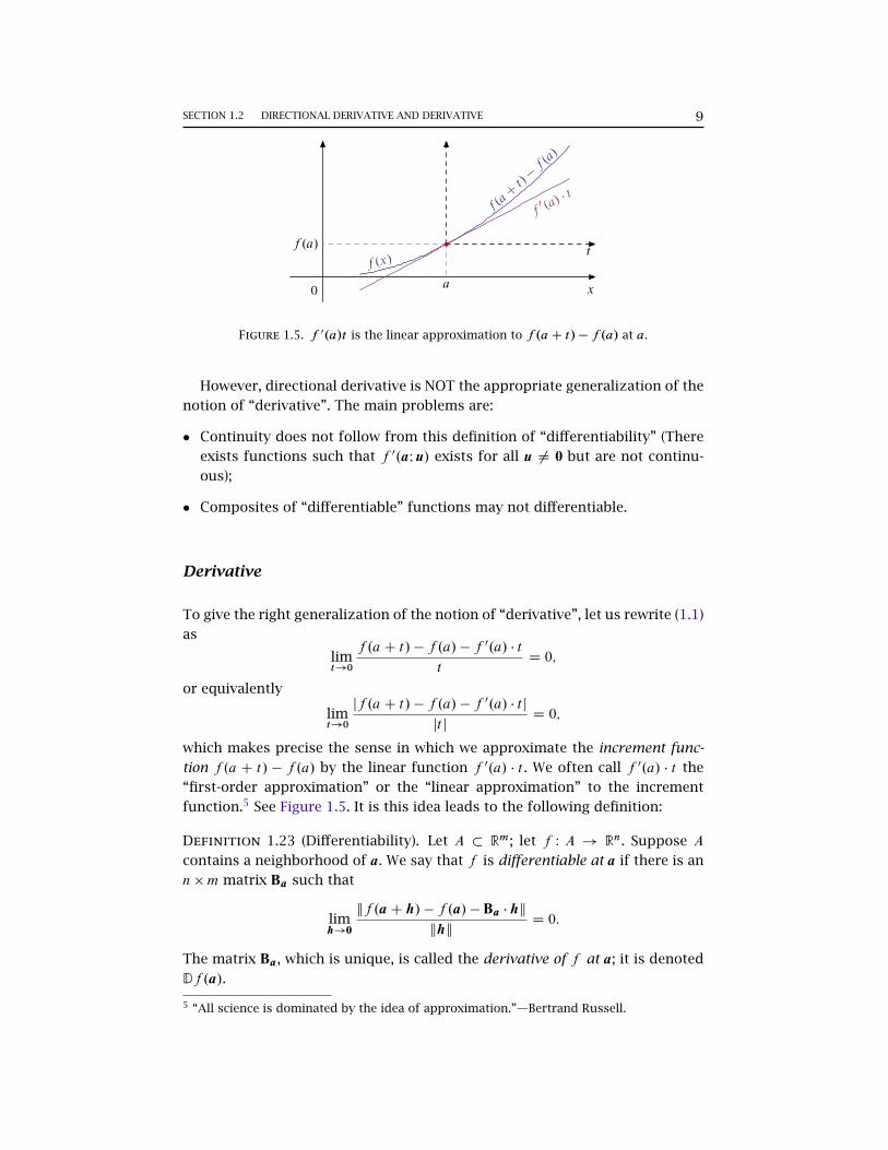
Figure 1.5. f 0.a/t is the linear approximation to f .aC t/� f .a/ at a.
However, directional derivative is NOT the appropriate generalization of the
notion of “derivative”. The main problems are:
� Continuity does not follow from this definition of “differentiability” (There
exists functions such that f 0.aIu/ exists for all u ¤ 0 but are not continu-
ous);
� Composites of “differentiable” functions may not differentiable.
Derivative
To give the right generalization of the notion of “derivative”, let us rewrite (1.1)
as
limt!0
f .aC t / � f .a/ � f 0.a/ � t
tD 0;
or equivalently
limt!0
jf .aC t / � f .a/ � f 0.a/ � t j
jt jD 0;
which makes precise the sense in which we approximate the increment func-
tion f .a C t / � f .a/ by the linear function f 0.a/ � t . We often call f 0.a/ � t the
“first-order approximation” or the “linear approximation” to the increment
function.5 See Figure 1.5. It is this idea leads to the following definition:
Definition 1.23 (Differentiability). Let A � Rm; let f W A ! Rn. Suppose A
contains a neighborhood of a. We say that f is differentiable at a if there is an
n �m matrix Ba such that
limh!0
kf .aC h/ � f .a/ � Ba � hk
khkD 0:
The matrix Ba, which is unique, is called the derivative of f at a; it is denoted
Df .a/.
5 “All science is dominated by the idea of approximation.”—Bertrand Russell.

10 CHAPTER 1 MULTIVARIABLE CALCULUS
Remark 1.24. Notice that h is a point of Rm and f .a C h/ � f .a/ � Ba � h is a
point of Rn, so the norm signs are essential. (Actually, it is enough to only take
the norm of h.)
Remark 1.25. The derivative Df .a/ depends on the point a as well as the
function f . We are not saying that there exists a B which works for all a, but
that for a fixed a such a B exists.
Example 1.26. Let f W Rm ! Rn be defined by the equation
f .x/ D A � x C b;
where A is an n �m matrix, and a 2 Rn. Then
limh!0
kf .aC h/ � f .a/ �A � hk
khkD 0I
that is, Df .a/ D A.
We now show that the definition of derivative is stronger than directional
derivative. In particular, we have:
Theorem 1.27. Let A � Rm; let f W A! Rn. If f is differentiable at a, then
f is continuous at a.
Proof. Let Ba D Df .a/. For h near 0 but different from 0, write
f .aC h/ � f .a/ D khk �
�f .aC h/ � f .a/ � Ba � h
khk
�C Ba � h:
Thus, kf .aC h/ � f .a/k ! 0 as h! 0. That is, f is continuous at a. ut
However, there is a nice connection between directional derivative and
derivative.
Theorem 1.28. Let A � Rm; let f W A! Rn. If f is differentiable at a, then
all the directional derivatives of f at a exist, and
f 0.aIu/ D Df .a/ � u:
Proof. Let Ba D Df .a/. Set h D tu in the definition of differentiability, where
t ¤ 0. Then by hypothesis,
0 D limt!0
kf .aC tu/ � f .a/ � Ba � tuk
ktuk
D limt!0
kf .aC tu/ � f .a/ � t � .Ba � u/k
jt j � kuk:
(1.2)

SECTION 1.3 PARTIAL DERIVATIVES AND THE JACOBIAN 11
If t # 0, we multiply (1.2) by kuk to conclude that
limt#0
f .aC tu/ � f .a/
t� Ba � u D 0:
If t " 0, we multiply (1.2) by �kuk to reach the same conclusion. Thus,
f 0.aIu/ D Ba � u. ut
I Exercise 1.29. Define f W R2 ! R by setting
f .x; y/ D
�0 if .x; y/ D .0; 0/x2y
x4 C y2if .x; y/ ¤ .0; 0/:
Show that all directional derivatives of f exist at .0; 0/, but that f is not differ-
entiable at .0; 0/.
I Exercise 1.30. Let f W R2 ! R be defined by f .x; y/ Dpjxyj. Show that f is
not differentiable at .0; 0/.
1.3 Partial Derivatives and the Jacobian
We now introduce the notion of the “partial derivatives” of a real-valued func-
tion. Let .e1; : : : ; em/ be the stand basis of Rm, i.e.,
e1 D .1; 0; 0; : : : ; 0/;
e2 D .0; 1; 0; : : : ; 0/;
: : :
em D .0; 0; : : : ; 0; 1/:
Definition 1.31 (Partial Derivatives). Let A � Rm; let f W A! R. We define the
j th partial derivative of f at a to be the directional derivative of f at a with
respect to the vector ej , provided this derivative exists; and we denote it by
Djf .a/. That is,
Djf .a/ D limt!0
f .aC tej / � f .a/
t:
Remark 1.32. It is important to note that Djf .a/ is the ordinary derivative of a
certain function; in fact, if g.x/ D f .a1; : : : ; aj�1; x; ajC1; : : : ; am/, then Djf .a/ D
g0.aj /. This means that Djf .a/ is the slope of the tangent line at .a; f .a// to
the curve obtained by intersecting the graph of f with the plane xi D ai with
i ¤ j . See Figure 1.6.
We now relate partial derivatives to the derivative in the case where f is a
real-valued function.

12 CHAPTER 1 MULTIVARIABLE CALCULUS
.a; b/
x1
x2
Figure 1.6. D1f .a; b/.
Theorem 1.33. Let A � Rm; let f W A! R. If f is differentiable at a, then
Df .a/ DhD1f .a/ D2f .a/ � � � Dmf .a/
i:
Proof. If f is differentiable at a, then Df .a/ is a .1 �m/-matrix. Let
Df .a/ Dh�1 �2 � � � �m
i:
It follows from Theorem 1.28 that
Djf .a/ D f0.aI ej / D Df .a/ � ej D �j : ut
Theorem 1.33 can be generalized as follows:

SECTION 1.4 GRADIENT AND ITS GEOMETRIC INTERPRETATION 13
Theorem 1.34. Let A � Rm; let f W A ! Rn. Suppose A contains a neigh-
borhood of a. Let fi W A! R be the i th component function of f , so that
f .x/ D
2664f1.x/:::
fn.x/
3775 :a. The function f is differentiable at a iff each component function fi is
differentiable at a.
b. If f is differentiable at a, then its derivative is the .n �m/-matrix whose
i th row is the derivative of the function fi . That is,
Df .a/ D
2664Df1.a/:::
Dfn.a/
3775 D2664
D1f1.a/ � � � Dmf1.a/:::
: : ::::
D1fn.a/ � � � Dmfn.a/
3775 :
I Exercise 1.35. Prove Theorem 1.34.
Definition 1.36 (Jocobian Matrix). Let A � Rm; let f W A ! Rn. If the partial
derivatives of the component functions fi of f exist at a, then one can form
the matrix that has Djfi .a/ as its entry in row i and column j . This matrix,
denoted by Jf .a/, is called the Jacobian matrix of f . That is,
Jf .a/ D
2664D1f1.a/ � � � Dmf1.a/
:::: : :
:::
D1fn.a/ � � � Dmfn.a/
3775 :Remark 1.37. The Jacobian encapsulates all the essential information regard-
ing the linear function that best approximates a differentiable function at a
particular point. For this reason it is the Jacobian which is usually used in
practical calculations with the derivative
Remark 1.38. If f is differentiable at a, then Jf .a/ D Df .a/. However, it is
possible for the partial derivatives, and hence the Jacobian matrix, to exist,
without it following that f is differentiable at a (see Exercise 1.29).
1.4 Gradient and Its Geometric Interpretation
Definition 1.39 (Gradient). Let A � Rm; let f W A ! R. Suppose A contains a
neighborhood of a. The gradient of f , denoted by Of .a/, is defined by

14 CHAPTER 1 MULTIVARIABLE CALCULUS
Of .a/´mXiD1
Dif .a/ � ei DhD1f .a/ D2f .a/ � � � Dmf .a/
i:
Remark 1.40. It follows from Theorem 1.33 that if f is differentiable at a,
then Of .a/ D Df .a/. The inverse does not hold; see Remark 1.38.
Let us now present a very important fact about gradient: the gradient is or-
thogonal to the level set.6 You will see this fact again and again. For simplicity,
we shall restrict ourselves on the case that f W R2 ! R.
Consider the gradient of f at .a; b/ 2 R2:
Of .a; b/ D .D1f .a; b/;D2f .a; b//:
We show that Of .a; b/ is orthogonal to the level set Lf .f .a; b// D f.x; y/ 2
R2 W f .x; y/ D f .a; b/g at .a; b/, which means that Of .a; b/ is orthogonal to the
tangent line at .a; b/. Let us begin with an example.
Example 1.41. Let f .x; y/ D x2Cy2. Then Of .1; 3/ D .2x; 2y/j.x;y/D.1;3/ D .2; 6/.The level set of f .1; 3/ D 10 is given by x2 C y2 D 10. Calculus yields
dy
dx
ˇ̌̌̌.1;3/
D �1
3:
Hence, the tangent line at .1; 3/ is given by
y D 3 �x � 1
3:
Then the result follows immediately; see Figure 1.7.
0 x
y Of .1; 3/ D .2; 6/
tangent line
.1; 3/
Lf .10/
Figure 1.7. The geometric interpretation of gradient.
6 Given a real-valued function f on A � Rm, the level set of f through c, where c is in therange, is
Lf .c/´˚x 2 A W f .x/ D c
:
We use level sets to help analyze functions in higher-dimensional spaces.

SECTION 1.5 CONTINUOUSLY DIFFERENTIABLE FUNCTIONS 15
0 x1
x2
Lf .c/
x
Of .x/
slope D �D1f .x/D2f .x/
Figure 1.8. The geometric interpretation of Of .x/.
We next turn to the more general analysis. Fix c in the range of f and take
an arbitrary point x D .x1; x2/ on the level set Lf .c/. If we change x1 and x2,
and are to remain on the level set, dx1 and dx2 must be such as to leave the
value of f unchanged at c. They must therefore satisfy
f 0.xI .dx1; dx2// D D1f .x/dx1 C D2f .x/dx2 D 0: (1.3)
By solving (1.3) for dx2=dx1, the slope of the level set through x will be (see
Figure 1.8)dx2dx1D �
D1f .x/
D2f .x/:
Since the slope of the vector Of .x/ D .D1f .x/;D2f .x// is D2f .x/=D1f .x/, we
obtain the desired result.
Remark 1.42. We will provide an physical interpretation of gradient in page
30.
1.5 Continuously Differentiable Functions
We know that mere existence of the partial derivatives does not imply differ-
entiability (see Exercise 1.29). If, however, we impose the additional condition
that these partial derivatives are continuous, then differentiability is assured.

16 CHAPTER 1 MULTIVARIABLE CALCULUS
Theorem 1.43. Let A be open in Rm. Suppose that the partial derivatives
Djfi .x/ of the component functions of f exist at each point x 2 A and are
continuous on A. Then f is differentiable at each point of A.
A function satisfying the hypotheses of this theorem is often said to be
continuously differentiable, or of class C1, on A.
Proof of Theorem 1.43. It suffices to show that each component function of
f is differentiable. Therefore we may restrict ourselves to the case of a real-
valued function f W A! R. Let a 2 A. Then
f .aC h/ � f .a/ Df .a1 C h1; a2; : : : ; am/ � f .a1; : : : ; am/
C f .a1 C h1; a2 C h2; a3; : : : ; am/ � f .a1 C h1; a2; : : : ; am/
C � � �
C f .a1 C h1; : : : ; am C hm/ � f .a1 C h1; : : : ; am�1 C hm�1; am/:
Note that D1f is the derivative of the function g defined by
g.x/ D f .x; a2; : : : ; am/:
Applying the mean-value theorem (Rudin, 1976, Theorem 5.10) to g we obtain
f .a1 C h1; a2; : : : ; am/ � f .a1; : : : ; am/ D h1 � D1f .b1; a2; : : : ; am/
for some b1 2 .a1; a1 C h1/. Similarly the i th term in the sum equals
hi � Dif .a1 C h1; : : : ; ai�1 C hi�1; bi ; aiC1; : : : ; am/ D hi � Dif .ci /
for some ci . Then
limh!0
ˇ̌̌̌ˇ̌f .aC h/ � f .a/ � mX
iD1
Dif .a/ � hi
ˇ̌̌̌ˇ̌
khkD lim
h!0
ˇ̌̌̌ˇ̌ mXiD1
�Dif .ci / � Dif .a/
�� hi
ˇ̌̌̌ˇ̌
khk
D limh!0
mXiD1
jDif .ci / � Dif .a/j �jhi j
khk
6 limh!0
mXiD1
jDif .ci / � Dif .a/j
D 0;
since Dif is continuous at a. ut
Remark 1.44. It follows from Theorem 1.43 that sin.xy/ and xy2 C zexy are
both differentiable since they are of class C1.

SECTION 1.6 THE CHAIN RULE 17
Let A � Rm and f W A ! Rn. Suppose that the partial derivative Djfi of the
component functions of f exist on A. These then are functions from A to R,
and we may consider their partial derivatives, which have the form
Dk.Djfi /µ Djkfi
and are called the second-order partial derivatives of f . Similarly, one defines
the third-order partial derivatives of the functions fi , or more generally the
partial derivatives of order r for arbitrary r .
Definition 1.45. If the partial derivatives of the function fi of order less than
or equal to r are continuous on A, we say f is of class C r on A. We say f is of
class C1 on A if the partials of the functions fi of all orders are continuous
on A.
Definition 1.46 (Hessian). Let a 2 A � Rm; let f W A! R be twice-differentiable
at a. The m � m matrix representing the second derivative of f is called the
Hessian of f , denoted Hf .a/:
Hf .a/ D
266664D11f .a/ D12f .a/ � � � D1mf .a/
D21f .a/ D22f .a/ � � � D2mf .a/:::
:::: : :
:::
Dm1f .a/ Dm2f .a/ � � � Dmmf .a/
377775 D D.Of /:
Remark 1.47. If f W A! R is of class C2, then the Hessian of f is a symmetric
matrix, i.e., Dijf .a/ D Dj if .a/ for all i; j D 1; : : : ; m and for all a 2 A. See Rudin
(1976, Corollary to Theorem 9.41, p. 236).
I Exercise 1.48. Find the Hessian of the Cobb-Douglas function
f .x; y/ D x˛yˇ :
1.6 The Chain Rule
We now extend the familiar chain rule to the current setting.
Theorem 1.49 (Chain Rule). Let A � Rm; let B � Rn. Let f W A ! Rn and
g W B ! Rp , with f .A/ � B . Suppose f .a/ D b. If f is differentiable at a,
and if g is differentiable at b, then the composite function g B f W A! Rp is
differentiable at a. Furthermore,
D.g B f /.a/ D Dg.b/ � Df .a/:

18 CHAPTER 1 MULTIVARIABLE CALCULUS
Proof. Omitted. See Spivak (1965, Theorem 2-2), Rudin (1976, Theorem 9.15),
or Munkres (1991, Theorem 7.1). ut
1.7 Quadratic Forms: Definite and Semidefinite Matrices
Definition 1.50 (Quadratic Form). Let A be a symmetric n � n matrix. A
quadratic form on Rn is a function QA W Rn ! R of the form
QA.x/ D x �Ax D
nXiD1
nXjD1
aijxixj :
Since the quadratic form QA is completely specified by the matrix A, we
henceforth refer to A itself as the quadratic form. Observe that if f is of class
C2, then the Hessian Hf of f defines a quadratic form; see Remark 1.47.
Definition 1.51. A quadratic form A is said to be
� positive definite if we have x �Ax > 0 for all x 2 Rn X f0g;
� positive semidefinite if we have x �Ax > 0 for all x 2 Rn;
� negative definite if we have x �Ax < 0 for all x 2 Rn X f0g;
� negative semidefinite if we have x �Ax 6 0 for all x 2 Rn.
1.8 The Implicit Function Theorem
Here is a typical problem:
“Assume that the equation x3yC2exy D 0 determines y as a differentiable functionof x. Find dy=dx.”
One solves this calculus problem by “looking at y as a function of x,” and
differentiating with respect to x. One obtains the equation
3x2y C x3dy
dxC 2exy
�y C x
@y
@x
�D 0;
which one solves for dy=dx. The derivative dy=dx is of course expressed in
terms of x and the unknown function y.
The case of an arbitrary function f is handled similarly. Supposing that
the equation f .x; y/ D 0 determines y as a differentiable function of x, say
y D g.x/, the equation f .x; g.x// D 0 is an identity. One applies the chain rule
to calculate@f
@xC@f
@yg0.x/ D 0;

SECTION 1.8 THE IMPLICIT FUNCTION THEOREM 19
so that
g0.x/ D �@f=@x
@f=@y;
where the partial derivatives are evaluated at the point .x; g.x//. Note that the
solution involves a hypothesis not given in the statement of the problem. In
order to find g0.x/, it is necessary to assume that @f=@y ¤ 0 at the point in
question.
It in fact turns out that @f=@y ¤ 0 is also sufficient to justify the assump-
tions we made in solving the problem. That is, if the function f .x; y/ has the
property that @f=@y ¤ 0 at a point .a; b/ that is a solution of the equation
f .x; y/ D 0, then this equation does determine y as a function of x, for x near
a, and this function of x is differentiable.
This result is a special case of a theorem called the implicit function theorem,
which we consider in this section.
Example 1.52. Consider the function f W R2 ! R defined by
f .x; y/ D x2 C y2 � 1:
If we choose .a; b/ with f .a; b/ D 0 and a ¤ ˙1, there are (Figure 1.9) open
intervals A containing a and B containing b with the following property: if x 2
A, there is a unique y 2 B with f .x; y/ D 0. We can therefore define a function
g W A! R by the condition g.x/ 2 B and f .x; g.x// D 0 (if b > 0, as indicated in
Figure 1.9, then g.x/ Dp1 � x2). For the function f we are considering there
is another number b1 such that f .a; b1/ D 0. There will also be an interval B1containing b1 such that, when x 2 A, we have f .x; g1.x// D 0 for a unique
g1.x/ 2 B1 (here g1.x/ D �p1 � x2). Both g and g1 are differentiable. These
functions are said to be defined implicitly by the equation f .x; y/ D 0.
If we choose a D 1 or �1 it is impossible to find any such function g defined
in an open interval containing a.
We now introduce the Implicit Function Theorem. Let E be open in RkCn;
let f W E ! Rn. Write f in the form f .x;y/ for x 2 Rk and y 2 Rn. Think
of the equation f .x;y/ D 0 as a system of n equations in k C n variables.
With .a;b/ 2 Rk � Rn as a given solution, i.e. f .a;b/ D 0, the theorem tells
us under what condition, we can solve for the variables y near b in terms of
the variables x, to obtain a unique continuously differentiable solution. The
new function g.x/ so obtained is said to be given by the equation f .x;y/ D 0
implicitly. That is why the theorem is so named.

20 CHAPTER 1 MULTIVARIABLE CALCULUS
0 x
y
graph of g
graph of g1f .x; y/ D 0
.a; b/B
B1
A
b
b1
a
Figure 1.9. Implicit function theorem.
Theorem 1.53 (Implicit Function Theorem). Let E � RkCn be open; let
f W E ! Rn be of class C r . Write f in the form f .x;y/ for x 2 Rk and
y 2 Rn. Suppose that .a;b/ is a point of E such that f .a;b/ D 0. Let M be
the n � n matrix
M D
266664DkC1f1.a;b/ DkC2f1.a;b/ � � � DkCnf1.a;b/
DkC1f2.a;b/ DkC2f1.a;b/ � � � DkCnf2.a;b/:::
:::: : :
:::
DkC1fn.a;b/ DkC2fn.a;b/ � � � DkCnfn.a;b/
377775 :
If det .M/ ¤ 0, then there is a neighborhood A of a 2 Rk and a unique
continuous function g W A! Rn such that g.a/ D b and
f .x; g.x// D 0
for all x 2 A. The function g is in fact of class C r .
Proof. The proof is too long to give here. You can find it from, e.g., Spivak
(1965, Theorem 2-12), Rudin (1976, Theorem 9.28), or Munkres (1991, Theo-
rem 2.9.2). ut
Example 1.54. Let f W R2 ! R be given by the equation

SECTION 1.8 THE IMPLICIT FUNCTION THEOREM 21
f .x; y/ D x2 � y3:
Then .0; 0/ is a solution of the equation f .x; y/ D 0. Because @f .0; 0/=@y D 0,
we do not expect to be able to solve this equation for y in terms of x near
.0; 0/. But in fact, we can; and furthermore, the solution is unique! However,
the function we obtain is not differentiable at x D 0. See Figure 1.10.
0 x
y
Figure 1.10. y is not differentiable at x D 0.
Example 1.55. Let f W R2 ! R be given by the equation
f .x; y/ D �x4 C y2:
Then .0; 0/ is a solution of the equation f .x; y/ D 0. Because @f .0; 0/=@y D 0, we
do not expect to be able to solve for y in terms of x near .0; 0/. In fact, however,
we can do so, and we can do so in such a way that the resulting function is
differentiable. However, the solution is not unique. See Figure 1.11.
Now the point .1; 1/ is also a solution to f .x; y/ D 0. Because @f .1; 1/=@y D 2,
one can solve this equation for y as a continuous function of x in a neighbor-
hood of x D 1. See Figure 1.11.
0 x
y
−2 −1 1 2
−1
1
Figure 1.11. Example 1.55.

22 CHAPTER 1 MULTIVARIABLE CALCULUS
Remark 1.56. We will use the Implicit Function Theorem in Theorem 2.10. The
theorem will also be used to derive comparative statics for economic models,
which we perhaps do not have time to discuss.
1.9 Homogeneous Functions and Euler’s Formula
Definition 1.57 (Homogeneous Function). A function f W Rn ! R is homoge-
neous of degree r (for r D : : : ;�1; 0; 1; : : :) if for every t > 0 we have
f .tx1; : : : ; txn/ D trf .x1; : : : ; xn/:
I Exercise 1.58. The function
f .x; y/ D Ax˛yˇ ; A; ˛; ˇ > 0;
is known as the Cobb-Douglas function. Check whether this function is homoge-
neous.
Theorem 1.59 (Euler’s Formula). Suppose that f W Rn ! R is homogeneous
of degree r (for some r D : : : ;�1; 0; 1; : : :) and differentiable. Then at any
x� 2 Rn we have
Of .x�/ � x� D rf .x�/:
Proof. By definition we have
f .tx�/ � t rf .x�/ D 0:
Differentiating with respect to t using the chain rule, we have
Of .tx�/ � x� D rt r�1f .x�/:
Evaluating at t D 1 gives the desired result. ut
Lemma 1.60. If f is homogeneous of degree r , its partial derivatives are homo-
geneous of degree r � 1.
I Exercise 1.61. Prove Lemma 1.60.
I Exercise 1.62. Let f .x; y/ D Ax˛yˇ with ˛ C ˇ D 1 and A > 0. Show that
Theorem 1.59 and Lemma 1.60 hold for this function.

2OPTIMIZATION IN RN
This chapter is based on Luenberger (1969, Chapters 8 & 9), Mas-Colell, Whin-
ston and Green (1995, Sections M.J & M.K), Sundaram (1996), Duggan (2010),
and Jehle and Reny (2011, Chapter A2).
2.1 Introduction
An optimization problem in Rn, or simply an optimization problem, is one where
the values of a given function f W Rn ! R are to be maximized or minimized
over a given set X � Rn. The function f is called the objective function and the
set X the constraint set. Notationally, we will represent these problems by
Maximize f .x/ subject to x 2 X;
and
Minimize f .x/ subject to x 2 X;
respectively. More compactly, we shall also write
max ff .x/ W x 2 Xg and min ff .x/ W x 2 Xg :
Example 2.1. (a) Let X D Œ0;1/ and f .x/ D x. Then the problem maxff .x/ W
x 2 Xg has no solution; see Figure 2.1(a).
(b) Let X D Œ0; 1� and f .x/ D x.1�x/. Then the problem maxff .x/ W x 2 Xg has
exactly one solution, namely x D 1=2; see Figure 2.1(b).
(c) Let X D Œ�1; 1� and f .x/ D x2. Then the problem maxff .x/ W x 2 Xg has
two solutions, namely x D �1 and x D 1; see Figure 2.1(c).
˘
Example 2.1 suggests that we shall talk of the set of solutions of the opti-
mization problem, which is denoted
23

24 CHAPTER 2 OPTIMIZATION IN RN
0 x
x
(a) No solution.
0 x1
x.1 � x/
(b) Exactly one solution.
0 x−1 1
x2
(c) Two solutions.
Figure 2.1. Example 2.1.
argmax ff .x/ W x 2 Xg D˚x 2 X W f .x/ > f .y/ for all y 2 X
:
We close this section by considering an optimization problem in economics.
Example 2.2. There are n commodities in an economy. There is a consumer
whose utility from consuming xi > 0 units of commodity i (i D 1; : : : ; n) is
given by u.x1; : : : ; xn/, where u W RnC ! R is the consumer’s utility function. The
consumer’s income is I > 0, and faces the price vector p D .p1; : : : ; pn/. His
budget set is given by (see Figure 2.2)
B.p; I /´˚x 2 RnC W p � x 6 I
:
The consumer’s objective is to maximize his utility over the budget set, i.e.,
Maximize u.x/ subject to x 2 B.p; I /:
0 x1
x2
B.p; I /
I=px1
I=px2
Figure 2.2. The budget set B.px1 ; px2 ; I /.

SECTION 2.2 UNCONSTRAINED OPTIMIZATION 25
2.2 Unconstrained Optimization
Definition 2.3 (Maximizer). Given X � Rn, f W X ! R, x 2 X , we say x is a
maximizer of f if
f .x/ D max ff .y/ W y 2 Xg :
We say x is a local maximizer of f if there is some " > 0 such that for all
y 2 X \B.xI "/ we have f .x/ > f .y/. And x is a strict local maximizer of f if
the latter inequality holds strictly.
First-Order Analysis
Recall that XB is the interior of X � Rn (Definition 1.13), and f 0.xIu/ is the
directional derivative of f at x with respect to u (Definition 1.21).
Theorem 2.4. Let X � Rn; let x 2 XB; let f W X ! R be differentiable at
x. If x is a local maximizer of f , then for every direction u 2 X we have
f 0.xIu/ D 0.
Proof. Suppose that x is an interior local maximizer and let u 2 X . Take
" > 0 such that B.xI "/ � X and f .x/ > f .y/ for all y 2 B.xI "/. In particular,
f .x/ > f .x C ˛u/ for ˛ 2 R small. Since f is differentiable at x, we have
f 0.xIu/ D lim˛#0
f .x C ˛u/ � f .x/
˛6 0;
and
f 0.xIu/ D lim˛"0
f .x C ˛u/ � f .x/
˛> 0:
Therefore, f 0.xIu/ D 0, as claimed. ut
Remark 2.5. If f is differentiable at x and x is an interior local maximizer of
f , then since f 0.xIu/ D Of .x/ � u (Theorem 1.28, Theorem 1.33 and Defini-
tion 1.39), we know that for all u
Of .x/ � u D 0;
which implies that Of .x/ D 0.
Definition 2.6 (Critical Point). A vector x 2 Rn such that Of .x/ D 0 is called
a critical point.
Example 2.7. Let X D R2 and f .x; y/ D xy�2x4�y2. The first order condition
is
Of .x; y/ D .y � 8x3; x � 2y/ D .0; 0/:

26 CHAPTER 2 OPTIMIZATION IN RN
0 x−1 1
2x3�3x2
Figure 2.3. x D 0 and x D 1 are local optima but not global optima.
Thus, the critical points are .x; y/ D .0; 0/; .1=4; 1=8/; .�1=4;�1=8/.
Second-Order Analysis
The first-order conditions for unconstrained local optima do not distinguish
between maxima and minima (see the following Example 2.9). To obtain such
a distinction in the behavior of f at an optimum, we need to examine the
behavior of the Hessian Hf of f (see Definition 1.46).
Theorem 2.8. Suppose f is of class C2 on X � Rn, and x 2 XB.
a. If f has a local maximum at x, then Hf .x/ is negative semidefinite.
b. If f has a local minimum at x, then Hf .x/ is positive semidefinite.
c. If Of .x/ D 0 and Hf .x/ is negative definite at some x, then x is a strict
local maximum of f on X .
d. If Of .x/ D 0 and Hf .x/ is positive definite at some x, then x is a strict
local minimum of f on X .
Proof. See Sundaram (1996, Section 4.6). ut
Example 2.9. Let f W R! R be defined by f .x/ D 2x3 � 3x2. It is easy to check
that f 2 C2 on R and there are two critical points: x D 0 and x D 1. Invoking
the second-order conditions, we get f 00.0/ D �6 and f 00.1/ D 6. Thus, the point
x D 0 is a strict local maximum of f on R, and the point x D 1 is a strict local
minimum of f on R; see Figure 2.3.

SECTION 2.3 EQUALITY CONSTRAINED OPTIMIZATION: LAGRANGE’S METHOD 27
However, there is nothing in the first- or second-order conditions that will
help determine whether these points are global optima. In fact, they are not:
global optima do not exist in this example, since limx!C1 f .x/ D C1 and
limx!�1 f .x/ D �1.
2.3 Equality Constrained Optimization: Lagrange’s
Method
First-Order Analysis
Lagrange’s Theorem
Theorem 2.10 (Lagrange’s Theorem). Let f W Rn ! R, and gi W Rn ! R be
C1 functions, where i D 1; : : : ; k. Suppose that x� is a local maximizer or
minimizer of f on the set
X ´ U \˚x 2 Rn W gi .x/ D 0; i D 1; : : : ; k
;
where U � Rn is open. Suppose also that the list of vectors
.Og1.x�/; : : : ;Ogk.x�// is linearly independent (this is called the constraint
qualification). Then, there exists a vector �� D .��1 ; : : : ; ��k/ 2 Rk such that
Of .x�/ DkXiD1
��i �Ogi .x�/:
Here we give a proof for the case of two variables and one constraint (This
proof is from Duggan 2010, Theorem 5.1). We are interested in this proof
partly because we will use the Implicit Function Theorem (Theorem 1.53). For
a general proof, see Sundaram (1996, Section 5.6).
Proof (Two variables, one constraint). We show that if
x� 2 argmax ff .x/ W g.x/ D 0g ;
and Og.x�/ ¤ 0, then there exists � 2 R such that
Of .x�/ D �Og.x�/: (2.1)
Without loss of generality, we assume that x� D 0 and D2g.x�/ ¤ 0. The
Implicit Function Theorem (Theorem 1.53) implies that in an open interval I
around x�1 D 0, we may then view the level set Lg.0/ as the graph of a function
' W I ! R such that for all z 2 I we have

28 CHAPTER 2 OPTIMIZATION IN RN
0 x1
x2
0 x1
x2
z
'.z/
. /I
Og.x�/Lg .0/
Figure 2.4. Proof of Lagrange’s Theorem.
g.z; '.z// D 0: (2.2)
See Figure 2.4. Notice that
0 D x� D .0; '.0//:
Furthermore, ' is continuously differentiable with derivative (by (2.2))
'0.z/ D �D1g.z; '.z//
D2g.z; '.z//: (2.3)
Because x� 2 U and U is open, we can choose the interval I small enough
that each .z; '.z// 2 U . Then z D 0 is a local maximizer of the unconstrained
problem
maxz2I
f .z; '.z//:
Then, by the first-order condition, we have
D1f .0/C D2f .0/ � '0.0/ D 0;
which implies (by (2.3))
D1f .0/ � D2f .0/ �D1g.0/
D2g.0/D 0: (2.4)
Defining
� DD2f .0/
D2g.0/;
we have

SECTION 2.3 EQUALITY CONSTRAINED OPTIMIZATION: LAGRANGE’S METHOD 29
�Og.0/ DD2f .0/
D2g.0/�
hD1g.0/ D2g.0/
iD
hD2f .0/D1g.0/
D2g.0/D2f .0/
iD
hD1f .0/ D2f .0/
iD Of .0/;
where the third equality follows from (2.4). ut
Geometric Interpretation
Let us consider an optimization problem on R2 and with one constraint:
maxx1;x2
f .x1; x2/ subject to g.x1; x2/ D 0: (2.5)
Consider the level sets Lf .c/ and Lg.0/. Recall that (see Section 1.4) for every
point x 2 Lf .c/, we have
dx2dx1
ˇ̌̌̌ˇalong Lf .c/
D �D1f .x/
D2f .x/; (2.6)
and for every point y 2 Lg.0/ we have
dy2dy1
ˇ̌̌̌ˇalong Lg.0/
D �D1g.y/
D2g.y/: (2.7)
It follows from Theorem 2.10 that if x� is a solution to (2.5), then
D1f .x�/ D ��D1g.x
�/;
D2f .x�/ D ��D2g.x
�/;
g.x�/ D 0:
Suppose that �� ¤ 0. Then we can rewrite the above conditions as follows:
D1f .x�/
D2f .x�/D
D1g.x�/
D2g.x�/(2.8)
g.x�/ D 0: (2.9)
The first equation (2.8) says that solution values of x1 and x2 will be at a
point where the slope of the level set for the objective function and the slope
of the level set for the constraint are equal. The second equation (2.9) tells us
we must also be on the level set of the constraint equation. See Figure 2.5.

30 CHAPTER 2 OPTIMIZATION IN RN
0 x1
x2
Lg .0/
Lf .y�/
Lf .y/
Slope at tangency D �D1f .x�/
D2f .x�/D �
D1g.x�/
D2g.x�/
x�
Figure 2.5. The first-order conditions for a solution to Lagrange’s prob-lem identify a point of tangency between a level set of the objective func-tion and the constraint.
The Constraint Qualification
We show that Theorem 2.10 fails without the constraint qualification.
Example 2.11. Let X D R, f .x/ D .xC1/2 and g.x/ D x2. Consider the problem
of maximizing f subject to g.x/ D 0. The maximizer is clearly x D 0. But
Dg.0/ D 0 and Df .0/ D 2, so there is no � such that Df .0/ D �Dg.0/.
The Lagrange Multipliers
The vector �� D .��1 ; : : : ; ��k/ in Theorem 2.10 is called the vector of Lagrange
multipliers corresponding to the local optimum x�. The i th multiplier ��i mea-
sures the sensitivity of the value of the objective function at x� to a small
relaxation of the i th constraint gi .
Physical Interpretation of Gradient ?
We now can provide a physical interpretation of gradient (Shastri, 2011). Con-
sider any linear functional ' W Rn ! R defined by '.x/ DPniD1 ˛ixi , and the
problem of finding its maxima on the unit sphere Sn�1 ´ fx 2 Rn W kxk D 1g.
The Lagrange multiplier function in this case is
L D
nXiD1
˛ixi � �
0@ nXiD1
x2i � 1
1A :

SECTION 2.3 EQUALITY CONSTRAINED OPTIMIZATION: LAGRANGE’S METHOD 31
Thus,
˛i D 2�xi for all i D 1; : : : ; n:
Now fix i 2 f1; : : : ; ng, and we have
xj D j̨
xi
˛ifor all j D 1; : : : ; n:
Therefore, for each i 2 f1; : : : ; ng
xi D ˙˛i�Pn
iD1 ˛2i
�1=2 : (2.10)
Now let f W U ! R be a C1 function in a neighborhood U of 0 2 Rn. Let
'.x/ D Df .0/ � x. To each v 2 Sn�1 we can consider the path .�"; "/! U given
by t 7! tv and look at the function t 7! f .tv/. The derivative of this map at 0 is
nothing by Df .0/ � v. Therefore, form (2.10), it follows that the extrema of the
function
v 7! Df .0/ � v DnXiD1
Dif .0/ � vi
occur at ˙Of .0/=kOf .0/k. Thus, Of is the direction in which the increment in
f is the maximum.
Lagrange’s Method
Let an equality-constrained optimization problem of the form
Maximize f .x/ subject to x 2 X D U \˚x 2 Rn W g.x/ D 0
; (2.11)
be give, where f W Rn ! R and g W Rn ! Rk are of C1 functions, and U � Rn is
open. We describe a procedure for using Theorem 2.10 to solve (2.11).
Step 1. Set up a function L W X � Rk ! R, called the Lagrangian, defined by
L.x;�/ D f .x/ �
kXiD1
�igi .x/:
The vector � D .�1; : : : ; �k/ 2 Rk is called the vector of Lagrange multipliers.
Step 2. Find all critical points of L.x;�/:
@L
@xi.x;�/ D Dif .x/ �
kX`D1
�`Dig`.x/ D 0; i D 1; : : : ; n (2.12)
@L
@�j.x;�/ D gj .x/ D 0; j D 1; : : : ; k: (2.13)
Define

32 CHAPTER 2 OPTIMIZATION IN RN
M ´˚.x;�/ W x 2 U , and .x;�/ satisfies (2.12) and (2.13)
:
Step 3. Evaluate f at each point x in the setnx 2 Rn W 9 � 2 Rk such that .x;�/ 2M
o:
Thus, we see that Lagrange’s method is a clever way of converting a maxi-
mization problem with constraints, to another maximization problem without
constraint, by increasing the number of variables.
Why the Lagrange’s Method typically succeeds in identifying the desired
optima? This is because the set of all critical points of L contains the set of
all local maximizers and minimizers of the objective function f on X at which
the constraint qualification is met. That is, if x� is a maximizer or minimizer
of f on X , and if the constraint qualification holds at x�, then there exists ��
such that .x�;��/ is a critical point of L.
We are not going to explain why the Lagrange’s method could fail (but see
Sundaram 1996, Section 5.4 for details).
Example 2.12. Consider the problem
max.x;y/2R2
nf .x; y/ D �x2 � y2
osubject to g.x; y/ D x C y � 1 D 0:
First, form the Lagrangian,
L.x; y; �/ D �x2 � y2 � �.x C y � 1/:
Then set all of its first-order partials equal to zero:
@L
@xD �2x � � D 0
@L
@yD �2y � � D 0
@L
@�D x C y � 1 D 0:
So the critical points of L is
.x�; y�; ��/ D .1=2; 1=2;�1/:
Hence, f .x�; y�/ D �1=2; see Figure 2.6.
I Exercise 2.13. A consumer purchases a bundle .x; y/ to maximize utility. His
income is I > 0 and prices are px > 0 and py > 0. His utility function is
u.x; y/ D xayb;
where a; b > 0. Find his optimal choice .x�; y�/.

SECTION 2.3 EQUALITY CONSTRAINED OPTIMIZATION: LAGRANGE’S METHOD 33
0 x
y
L f.�2/
L f.�1/
L f.�1=2/
x�
Lg .0/
Figure 2.6. Lagrange’s method.
Lagrange’s Theorem Is Not Sufficient
Lagrange’s Theorem (Theorem 2.10) only gives us a necessary—not a suffi-
cient—condition for a constrained local maximizer. To see why the first order
condition is not generally sufficient, consider the following example.
Example 2.14. Let U D R2, f .x; y/ D x C y2, and g.x; y/ D x � 1. Consider the
problem
max.x;y/2R2
f .x; y/
s.t. g.x; y/ D 0:
Observe that .x�; y�/ D .1; 0/ satisfies the constraint g.x�; y�/ D 0, and the
constraint qualification is also satisfied. Furthermore, the first-order condition
from Lagrange’s Theorem is satisfied at .x�; y�/ D .1; 0/. This is because
Of .1; 0/ D .1; 0/ and Og.1; 0/ D .1; 0/:
Hence, by letting � D 1 we have Of .1; 0/ D �Og.1; 0/.However, .1; 0/ is NOT a constrained local maximizer: for arbitrarily small
" > 0, we have g.1; "/ D 0 and f .1; "/ D 1C "2 > 1 D f .1; 0/. See Figure 2.7.

34 CHAPTER 2 OPTIMIZATION IN RN
0 x
y
.1; 0/
.1; "/
Lg .0/
Lf .1/
Lf .1C "2/
Figure 2.7. The Lagrange’s Theorem is not sufficient.
Second-Order Analysis
We probably do not have time to discus the second-order conditions. See Jehle
and Reny (2011, Section A2.3.4) and Sundaram (1996, Section 5.3).
2.4 Inequality Constrained Optimization: Kuhn-Tucker
Theorem
We now consider maximization defined by inequality constraints. The con-
straint set will now be
X D U \˚x 2 Rn W hi .x/ 6 0; i D 1; : : : ; `
;
where U � Rn is open, and hi W Rn ! R for every i D 1; : : : ; `. Given x 2 Rn, we
say the i th constraint is binding if hi .x/ D 0, and slack if hi .x/ < 0.
First-Order Analysis
Example 2.15. Figure 2.8 illustrates a problem with two inequality constraints
and depicts three possibilities, depending on whether none, one, or two con-
straints are binding.

SECTION 2.4 INEQUALITY CONSTRAINED OPTIMIZATION: KUHN-TUCKER THEOREM 35
0 x1
x2
0 x1
x2
0 x1
x2
0 x1
x2
Of .y/
Oh1.y/
Oh2.z/
Oh1.z/
Of .z/
h1 D 0
h2 D 0
x
Df .x/ D 0
y
z
Figure 2.8. Inequality constrained optimization.
� In the first case, we could have a constrained local maximizer such as x,
for which no constraints bind. Such a vector must be a critical point of the
objective function.
� In the second case, we could have a single constraint binding at a con-
strained local maximizer such as y , and here the gradients of the objective
and constraint are collinear. As we will see, these gradients actually point in
the same direction.
� Lastly, we could have a constrained local maximizer such as z, where both
constraints bind. Here, the gradient of the objective is not collinear with the
gradient of either constraint, and it may appear that no gradient restriction
is possible. But in fact, Of .z/ can be written as a linear combination of
Oh1.z/ and Oh2.z/ with non-negative weights.
The restrictions evident in Figure 2.8 are formalized in the next theorem.

36 CHAPTER 2 OPTIMIZATION IN RN
Oh1.x�/
Oh2.x�/
Of .x�/
x�
Figure 2.9. Kuhn-Tucker Theorem.
Theorem 2.16 (Kuhn-Tucker Theorem). Let f W Rn ! R and hi W Rn ! R be
of C1 class functions, i D 1; : : : ; `. Suppose x� is a local maximizer of f on
X D U \˚x 2 Rn W hi .x/ 6 0; i D 1; : : : ; `
;
where U is an open subset in Rn. Suppose that the first k, where k 6 `, con-
straints are the binding ones at x�, and assume the gradients of the binding
constraints, fOh1.x�/; : : : ;Ohk.x�/g, are linear independent (this is called
the constraint qualification). Then there exists a vector �� D .��1 ; : : : ; ��`/ 2
R` such that
��i > 0 and ��i hi .x�/ D 0 for all i D 1; : : : ; `; (KT-1)
Of .x�/ DX̀iD1
�iOhi .x�/: (KT-2)
Proof. See Sundaram (1996, Section 6.5). ut
Remark 2.17. Geometrically, the first-order condition from the Kuhn-Tucker
Theorem means that the gradient of the objective function, Of .x�/, is con-
tained in the “semi-positive cone” generated by the gradients of binding con-
straints, i.e., it is contained in the set8<:X̀iD1
˛iOhi .x�/ W ˛1; : : : ; ˛` > 0
9=; ;depicted in Figure 2.9.
Remark 2.18. Condition (KT-1) in Theorem 2.16 is called the condition of com-
plementary slackness: if hi .x�/ < 0 then ��i D 0; if ��i > 0 then hi .x�/ D 0.

SECTION 2.4 INEQUALITY CONSTRAINED OPTIMIZATION: KUHN-TUCKER THEOREM 37
The Kuhn-Tucker Multipliers
The vector �� in Theorem 2.16 is called the vector of Kuhn-Tucker multipliers
corresponding to the local maximizer x�. The Kuhn-Tucker multipliers mea-
sure the sensitivity of the objective function at x� to relaxations of the various
constraints:
� If hi .x�/ < 0, then the i th constraint is already slack, so relaxing it further
will not help raise the value of the objective function, and ��i must be zero.
� If hi .x�/ D 0, then relaxing the i th constraint may help increase the value of
the maximization exercise, so we have ��i > 0.
Two Differences
There are two important differences from the case of equality constraints (see
Theorem 2.10 and Theorem 2.16):
� The constraint qualification now holds only for the gradients of binding
constraints. (With equality constraints, every constraint is binding, but now
some may not be.)
� The multipliers are non-negative. This difference comes from the fact that
now only the inequality hi .x/ 6 0 needs to be maintained, so relaxing the
constraint never hurts.
The Constraint Qualification
As with the analogous condition in Theorem 2.10 (see Example 2.11), here we
show that the constraint qualification in Theorem 2.16 is essential.
Example 2.19. Consider the following maximization problem
max ff .x; y/ D xg
s.t. h1.x; y/ D �.1 � x/3C y 6 0
h2.x; y/ D �x 6 0h3.x; y/ D �y 6 0:
See Figure 2.10. Clearly the solution is .x�; y�/ D .1; 0/. At this point we have
Oh1.1; 0/ D .0; 1/; Oh3.1; 0/ D .0;�1/ and Of .1; 0/ D .1; 0/:
Since x� > 0, it follows from the complementary slackness condition (KT-1)
that ��2 D 0. But now (KT-2) fails: for any �1 > 0 and �3 > 0, we have
�1Oh1.1; 0/C �3Oh3.1; 0/ D .0; �1 � �3/ ¤ Of .1; 0/:

38 CHAPTER 2 OPTIMIZATION IN RN
0 x
y
1
Lf .1=2/ Lf .1/
Lh1 .0/
Oh3.1; 0/
Of .1; 0/
Oh1.1; 0/
Figure 2.10. The constraint qualification fails at .1; 0/.
This is because the constraint qualification fails at .1; 0/: There are two
binding constraints at .x�; y�/ D .1; 0/, namely h1 and h3, and the gradients
Oh1.1; 0/ and Oh3.1; 0/ are colinear. Certainly Of .1; 0/ cannot be contained in
the cone generated by Oh1.1; 0/ and Oh3.1; 0/; see Remark 2.17.
The Lagrangian
As with equality constraints, we can define the Lagrangian L W Rn � R` ! R by
L.x;�/ D f .x/ �X̀iD1
�ihi .x/;
and then condition (KT-2) from Theorem 2.16 is the requirement that x is a
critical point of the Lagrangian given multipliers �1; : : : ; �`.
Let us consider a numerical example.
Example 2.20. Consider the problem
maxnf .x; y/ D x2 � y
os.t. h.x; y/ D x2 C y2 � 1 6 0:
Set the Lagrangian:
L.x; y; �/ D x2 � y � �.x2 C y2 � 1/:
The critical points of L are the solutions .x; y; �/ to

SECTION 2.4 INEQUALITY CONSTRAINED OPTIMIZATION: KUHN-TUCKER THEOREM 39
0 x
y
0 x
y
Lf.1/
Lf.5=4/
Lh .0/
.�p3=4;�1=2/ .
p3=4;�1=2/
Figure 2.11. A numerical example.
2x � 2�x D 0 (2.14)
�1 � 2�y D 0 (2.15)
� > 0 (2.16)
x2 C y2 � 1 6 0 (2.17)
�.x2 C y2 � 1/ D 0: (2.18)
For (2.14) to hold, we must have x D 0 or � D 1.
� If � D 1, then from (2.15) we have y D �1=2, and from (2.18) we have
x D ˙p3=2. That is,
.x; y; �/ D
˙
p3
2;�1
2; 1
!:
We thus have f .x; y/ D 5=4; see Figure 2.11.
� Now suppose that x D 0. Then � > 0 by (2.15). Hence h is binding: x2 C y2 �
1 D 0, and so y D ˙1. Since (2.15) implies that y D 1 is impossible, we have
.x; y; �/ D
�0;�1;
1
2
�:
At this critical point, we have f .0;�1/ D 1 < 5=4, which means that
.0;�1; 1=2/ cannot be a solution. Since there are no other critical points,
it follows that there are exactly two solutions to the maximization problem,
namely .x�; y�/ D .˙p3=2;�1=2/.
I Exercise 2.21. Let U D R2; let

40 CHAPTER 2 OPTIMIZATION IN RN
f .x; y/ D .x � 1/2 C y2;
and let
h.x; y/ D 2kx � y2 6 0; k > 0:
Solve the maximization problem
max ff .x; y/ W h.x; y/ 6 0g :
Example 2.22. Consider a consumer’s problem:
max.x;y/2R2
fu.x; y/ D x C yg
s.t. h1.x; y/ D �x 6 0h2.x; y/ D �y 6 0h3.x; y/ D pxx C pyy � I 6 0;
(2.19)
where px ; py ; I > 0.
We first identify all possible combinations of constraints that can, in princi-
ple, be binding at the optimum. There are eight combinations to be check:
¿; h1; h2; h3; .h1; h2/; .h1; h3/; .h2; h3/; and .h1; h2; h3/:
Of these, the last one can be ruled out, since h1 D h2 D 0 implies that h3 < 0.
Moreover, since u is strictly increasing in both arguments, it is obvious that
h3 D 0. So we only need to check three combinations: .h1; h3/, .h2; h3/, and h3.
� If the optimum occurs at a point where only h1 and h3 are binding, then�Oh1.x; y/;Oh3.x; y/
�D�.�1; 0/; .px ; py/
�is linear independent. So the constraint qualification holds at such a point.
� Similarly, the constraint qualification holds if only .h2; h3/ bind.
� If h3 is the only binding constraint, then Oh3.x; y/ D .px ; py/ ¤ 0; that is,
the constraint qualification holds.
I Exercise 2.23. Solve the problem of (2.19).
Second-Order Analysis
We probably do not have time to discus the second-order conditions. See Dug-
gan (2010, Section 6.3).

SECTION 2.5 ENVELOP THEOREM 41
2.5 Envelop Theorem
Let A � R. The graph of a real-valued function f on A is a curve in the R2
plane, and we shall also refer to the curve itself as f . Given a one-dimensional
parametrized family of curves f˛ W A ! R, where ˛ runs over some interval,
the curve h W A! R is the envelope of the family if
� each point on the curve h is tangent to the graph of one of the curves f˛and
� each curve f˛ is tangent to h.
(See, e.g., Apostol 1967, p. 342 or Zorich 2004b, p. 252 for this definition.) That
is, for each ˛, there is some q and also for each q, there is some ˛, satisfying˚f˛.q/ D h.q/
f 0˛.q/ D h0.q/:
We may regard h as a function of ˛ if the correspondence between curves and
points on the envelope is one-to-one.
An Envelopment Theorem for Unconstrained Maximization
Consider now an unconstrained parametrized maximization problem. Let
x�.q/ be the value of the control variable x that maximizes f .x; q/, where q
is our parameter of interest. For some fixed x, the function
'x.q/´ f .x; q/
defines a curve. We also define the value function
V.q/´ f�x�.q/; q
�D max
x'x.q/:
Under appropriate conditions, the graph of the value function V will be the
envelope of the curves 'x . “Envelope theorems” in maximization theory are
concerned with the tangency conditions this entails.
Example 2.24. Let
f .x; q/ D q � .x � q/2 C 1; x; q 2 Œ0; 2�:
Then given q, the maximizing x is given by x�.q/ D q, and V.q/ D q C 1.
For each x, the function 'x is given by
'x.q/ D q � .x � q/2C 1:

42 CHAPTER 2 OPTIMIZATION IN RN
0 q
'x.q/
1 2
1
2
3
xD0
xD0:2
xD0:4
xD0:6
xD0:8
xD1
(a) The family of curves f'x.q/ W x D0; 0:2; : : : ; 2g.
0 q
V.q/
1 2
1
2
3
V.q/ DqC1
(b) The envelop.
Figure 2.12. The graph of V is the envelope of the family of graphs ofthe functions 'x .
The graphs of these functions and of V are shown for selected values of x
in Figure 2.12. Observe that the graph of V is the envelope of the family of
graphs of the functions 'x . Consequently the slope of V is the slope of the 'xto which it is tangent, that is,
V 0.q/ D@'x
@q
ˇ̌̌̌xDx�.q/Dq
D@f
@q
ˇ̌̌̌xDx�.q/Dq
D 1C 2.x � q/jxDx�.q/Dq D 1:
This last observation is one version of the Envelope Theorem.
An Envelope Theorem for Constrained Maximization
Consider the maximization problem,
maxx2Rn
f .x; q/ s.t. gi .x; q/ D 0; i D 1; : : : ; m; (2.20)
where x is a vector of choice variables, and q D .q1; : : : ; q`/ 2 R` is a vector of
parameters that may enter the objective function, the constraints, or both.
Suppose that for each q there exists a unique solution x.q/. Furthermore,
we assume that the objective function f W Rn ! R, constraints gi W Rn � R` ! R
(i D 1; : : : ; m), and solutions x W R` ! Rn are differentiable in the parameter q.

SECTION 2.5 ENVELOP THEOREM 43
Then, for every parameter q, the maximized value of the objective function
is f .x.q/; q/. This defines a new function, V W R` ! R, called the value function.
Formally,
V.q/´ maxx2Rn
ff .x; q/ W gi .x; q/ D 0; i D 1; : : : ; mg : (2.21)
Theorem 2.25 (Envelope Theorem). Consider the value function V.q/ for
the problem (2.20). Let .�1; : : : ; �m/ be values of the Lagrange multipliers
associated with the maximizer solution x. Nq/ at Nq. Then for each k D 1; : : : ; `,
@V. Nq/
@qk
D@f .x. Nq/; Nq/
@qk
�
mXjD1
�j@gj .x. Nq/; Nq/
@qk
(2.22)
Proof. By definition, V.q/ D f .x.q/; q/ for all q. Using the chain rule, we have
@V. Nq/
@qk
D
nXiD1
"@f .x. Nq/; Nq/
@xi
@xi . Nq/
@qk
#C@f .x. Nq/; Nq/
@qk
:
It follows from Theorem 2.10 that
@f .x. Nq/; Nq/
@xiD
mXjD1
�j@gj .x. Nq/; Nq/
@xi:
Hence,
@V. Nq/
@qk
D
nXiD1
"@f .x. Nq/; Nq/
@xi
@xi . Nq/
@qk
#C@f .x. Nq/; Nq/
@qk
D
nXiD1
2640@ mXjD1
�j@gj .x. Nq/; Nq/
@xi
1A @xi . Nq/
@qk
375C @f .x. Nq/; Nq/
@qk
D
nXjD1
�j
nXiD1
"@gj .x. Nq/; Nq/
@xi
@xi . Nq/
@qk
#C@f .x. Nq/; Nq/
@qk
:
Finally, since gj .x.q/; q/ D 0 for all q, we have
nXiD1
"@gj .x. Nq/; Nq/
@xi
@xi . Nq/
@qk
#C@gj .x. Nq/; Nq/
@qk
D 0:
Combining, we get (2.22). ut
Let us consider an example.
Example 2.26. We are given the problem
max.x;y/2R2
ff ..x; y/; q/ D xyg s.t. g..x; y/; q/ D 2x C 4y � q D 0:

44 CHAPTER 2 OPTIMIZATION IN RN
Forming the Lagrangian, we get
L D xy � �.2x C 4y � q/;
with first-order conditions:
y � 2� D 0
x � 4� D 0
q � 2x � 4y D 0:
(2.23)
These solve for x.q/ D q=4, y.q/ D q=8 and �.q/ D q=16. Thus,
V.q/ D x.q/y.q/ Dq2
32:
Differentiating V.q/ with respect to q we get
V 0.q/ Dq
16:
Now let us verify this using the Envelope Theorem. The theorem tells us that
V 0.q/ D@f ..x.q/; y.q//; q/
@q� �.q/
@g..x.q/; y.q//; q/
@qD �.q/ D
q
16:
Example 2.27. Consider a consumer whose utility function u W RnC ! R is
strictly increasing in every commodity i D 1; : : : ; n. Then this consumer’s prob-
lem is
maxu.x/ s.t.nXiD1
xipi D I:
The Lagrangian is
L.x; �/ D u.x/ � �
0@I � nXiD1
xipi
1A :It follows from Theorem 2.25 that
V 0.I / [email protected]; �/
@ID �:
That is, � measures the marginal utility of income.
Integral Form Envelope Theorem
The Envelope theorems we introduced so far rely on assumptions that are not
satisfactory for applications, e.g., mechanism design. Unfortunately, it is too
technique to develop the more advanced treatment of the Envelope Theorem.
We refer the reader to Milgrom and Segal (2002) and Milgrom (2004, Chapter
3) for the integral form Envelope Theorem.

3CONVEX ANALYSIS IN RN
Rockafellar (1970) is the classical reference for finite-dimensional convex
analysis. As for infinite-dimensional convex analysis, Luenberger (1969) is an
excellent text.
To understand the material what follows, it is necessary that the reader have
a good background in Multivariable Calculus (Chapter 1) and Linear Algebra.
In this chapter, we will exclusively consider convexity in Rn for concreteness,
but much of the discussion here generalizes to infinite dimensional vector
spaces. You can consult Berkovitz (2002), Ok (2007, Chapter G) and Royden
and Fitzpatrick (2010, Chapter 6).
3.1 Convex Sets
Definition 3.1 (Convex Set). A subset C � Rn is convex if for every pair of
points x1;x2 2 C , the line segment
Œx1;x2�´ fx W x D �x1 C .1 � �/x2; 0 6 � 6 1g
belongs to C .
I Exercise 3.2. Sketch the following sets in R2 and determine from figure which
sets are convex and which are not:
a.n�x; y
�W x2 C y2 6 1
o,
b.n�x; y
�W 0 < x2 C y2 6 1
o,
c.n�x; y
�W y > x2
o,
d.n�x; y
�W jxj Cjyj 6 1
o, and
e.n�x; y
�W y > 1
ı1C x2
o.
45
46 CHAPTER 3 CONVEX ANALYSIS IN RN
(0, 1, 0)
(1, 0, 0)
(0, 0, 1)
(0, 1, 0)
(1, 0, 0)
(0, 0, 1)
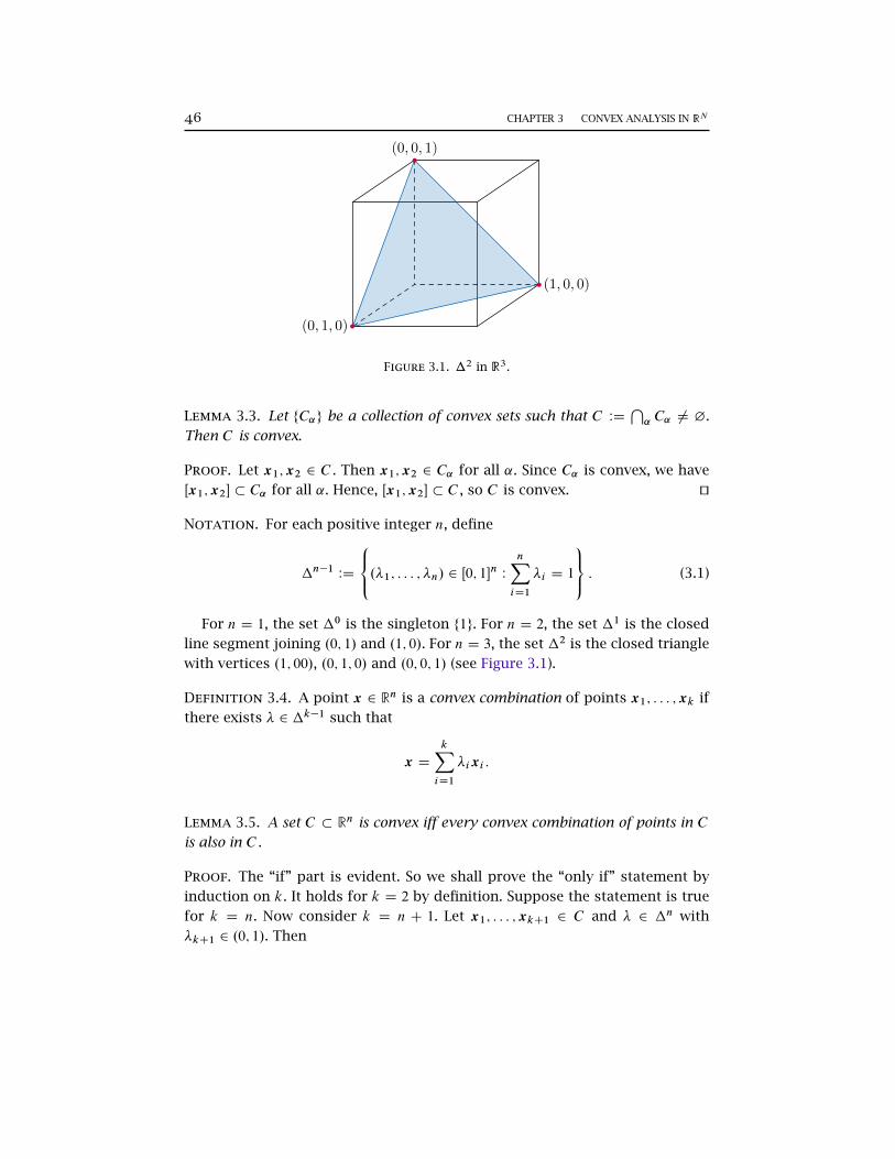
Figure 3.1. �2 in R3.
Lemma 3.3. Let fC˛g be a collection of convex sets such that C ´T˛ C˛ ¤ ¿.
Then C is convex.
Proof. Let x1;x2 2 C . Then x1;x2 2 C˛ for all ˛. Since C˛ is convex, we have
Œx1;x2� � C˛ for all ˛. Hence, Œx1;x2� � C , so C is convex. ut
Notation. For each positive integer n, define
�n�1´
8<:.�1; : : : ; �n/ 2 Œ0; 1�n WnXiD1
�i D 1
9=; : (3.1)
For n D 1, the set �0 is the singleton f1g. For n D 2, the set �1 is the closed
line segment joining .0; 1/ and .1; 0/. For n D 3, the set �2 is the closed triangle
with vertices .1; 00/, .0; 1; 0/ and .0; 0; 1/ (see Figure 3.1).
Definition 3.4. A point x 2 Rn is a convex combination of points x1; : : : ;xk if
there exists � 2 �k�1 such that
x D
kXiD1
�ixi :
Lemma 3.5. A set C � Rn is convex iff every convex combination of points in C
is also in C .
Proof. The “if” part is evident. So we shall prove the “only if” statement by
induction on k. It holds for k D 2 by definition. Suppose the statement is true
for k D n. Now consider k D n C 1. Let x1; : : : ;xkC1 2 C and � 2 �n with
�kC1 2 .0; 1/. Then

SECTION 3.2 SEPARATION THEOREM 47
x D
nC1XiD1
�ixi
D
0@ nXjD1
�j
1A24 nXiD1
�iPnjD1 �j
!xi
35C �kC1xkC12 C: ut
Let A � Rn, and let A be the class of all convex subsets of Rn that contain
A. We have A ¤ ¿—after all, Rn 2 A. Then, by Lemma 3.3,T
A is a convex
set in Rn that contains A. Clearly, this set is the smallest (that is, �-minimum)
convex subset of Rn that contains A.
Definition 3.6. The convex hull of A, denoted by cov.A/, is the intersection
of all convex sets containing A.
I Exercise 3.7. For a given set A, let K.A/ denote the set of all convex combi-
nations of points in A. Show that K.A/ is convex and A � K.A/.
Theorem 3.8. Let A � Rn. Then cov.A/ D K.A/.
Proof. Let A be the family of convex sets containing A. Since cov.A/ DT
A
and K.A/ 2 A (Exercise 3.7), we have cov.A/ � K.A/.
To prove the reverse inclusion relation, take an arbitrary C 2 A. Then A �
C . It follows from Lemma 3.5 that K.A/ � C . Hence K.A/ �T
A D cov.A/. ut
3.2 Separation Theorem
This section is devoted to the establishment of separation theorems. In some
sense, these theorems are the fundamental theorems of optimization theory.
For simplicity, we restrict our analysis on Rn.
Definition 3.9. A hyperplane Hˇa in Rn is defined to be the set of points that
satisfy the equation ha;xi D ˛. Thus,
Hˇa ´
˚x 2 Rn W ha;xi D ˇ
:
The vector a is said to be a normal to the hyperplane.
Remark 3.10. Geometrically, a hyperplane Hˇa in Rn is a translation of an
.n � 1/-dimensional subspace (an affine manifold). Algebraically, it is a level
set of a linear functional. For an excellent explanation about hyperplanes, see
Luenberger (1969, Section 5.12).

48 CHAPTER 3 CONVEX ANALYSIS IN RN
Hˇa
a
Half-space below Hˇa
Half-space above Hˇa
Figure 3.2. Hyperplane and half-spaces.
A hyperplane Hˇa divides Rn into two half spaces, one on each side of H
ˇa .
The set fx 2 Rn W ha;xi > ˇg is called the half-space above the hyperplane Hˇa ,
and the set fx 2 Rn W ha;xi 6 ˇg is called the half-space below the hyperplane
Hˇa ; see Figure 3.2.
It therefore seems natural to say that two sets X and Y are separated by
a hyperplane Hˇa if they are contained in different half spaces determined by
Hˇa . We will introduce two separation theorems.
Theorem 3.11 (A First Separation Theorem). Let C be a closed and convex
subset of Rn; let y 2 Rn X C . Then there exists a vector a 2 Rn with a ¤ 0,
and a scalar ˇ 2 R such that ha;yi > ˇ and ha;xi < ˇ for all x 2 C .
To motivate the proof, we argue heuristically from Figure 3.3, where C is
assumed to have a tangent at each boundary point. Draw a line from y to x�,
the point of C that is closest to y . The vector y � x� is orthogonal to C in
the sense that y � x� is orthogonal to the tangent line at x�. The tangent line,
which is exactly the set fz 2 Rn W hy � x�; z � x�i D 0g, separates y and C . The
point x� is characterized by the fact that hy � x�;x � x�i 6 0 for all x 2 C .
If we move the tangent line parallel to itself so as to pass through a point
x0 2 .x�;y/, we are done. We now justify these steps in a series of claims.
Claim 1. Let C be a convex subset of Rn and let y 2 Rn X C . If there exists a
point in C that is closest to y , then it is unique.
Proof. Suppose that there were two points x1 and x2 of C that were closest
to y . Then .x1 C x2/=2 2 C since C is convex, and so1
1 For a set X � Rn, the function d.y;X/ is the distance from y to X defined by
d.y;X/ D infx2Xky � xk:

SECTION 3.2 SEPARATION THEOREM 49
Hˇa
y
a
C
x�
x
y � x�
x � x�
Figure 3.3. The separating hyperplane theorem.
d.y; C / 6 x1 C x22
� y
D
12 �.x1 � y/C .x2 � y/�
61
2kx1 � yk C
1
2kx2 � yk
D d.y; C /:
Hence the triangle inequality holds with equality. It follows from Exercise 1.8
that there exists � > 0 such that x1�y D �.x2�y/. Clearly, � ¤ 0; for otherwise
x1 � y D 0 implies that y D x1 2 C . Then � D 1 since kx1 � yk D kx2 � yk D
d.y; C /. But then x1 D x2.
Claim 2. Let C be a closed subset of Rn and let y 2 Rn X C . Then there exists
a point x� 2 C that is closest to y .
Proof. Take an arbitrary point x0 2 C . Let r > kx0�yk. Then C1´ B.yI r/\C
is nonempty (at least x0 is in the intersection), closed, and bounded and hence
is compact. The function x 7! kx � yk is continuous on C1 and so attains its
minimum at some point x� 2 C1, i.e.,
kx� � yk 6 kx � yk for all x 2 C1:
For every x 2 C X C1, we have
kx � yk > r > kx0 � yk > kx� � yk;
since x0 2 C1.
Claim 3. Let C be a convex subset of Rn and let y 2 Rn X C . Then x� 2 C is a
closest point in C to y iff˝y � x�;x � x�
˛6 0 for all x 2 C: (3.2)
50 CHAPTER 3 CONVEX ANALYSIS IN RN
Proof. Let x� 2 C be a closest point to y and let x 2 C . Since C is convex, we
have
Œx�;x�´˚z.t/ 2 Rn W z.t/ D x� C t .x � x�/; t 2 Œ0; 1�
� C:
Let
g.t/´ kz.t/ � yk2 D˝x� C t .x � x�/ � y;x� C t .x � x�/ � y
˛D
nXiD1
�x�i � yi C t .xi � x
�i /�2:
Observe that g.0/ D x�. Since g is continuously differentiable on .0; 1� and
x� 2 argminx2C kx � yk, we have g0C.0/ > 0. Since
g0.t/ D 2
nXiD1
�x�i � yi C t .xi � x
�i /�.xi � x
�i /
D 2
24� nXiD1
.yi � x�i /.xi � x
�i /C t
nXiD1
.xi � x�i /2
35D 2
h�˝y � x�;x � x�
˛C tkx � x�k2
i:
(3.3)
Letting t # 0 we get (3.2).
Conversely, suppose that (3.2) holds. Take an arbitrary x 2 C X fx�g. It
follows from (3.3) that if t 2 .0; 1� then
g0.t/ D 2h�˝y � x�;x � x�
˛C tkx � x�k2
i> 2tkx � x�k2 > 0:
That is, g is strictly increasing on Œ0; 1�. Thus, g.1/ D kx � yk > kx� � yk D
g.0/.
Proof of Theorem 3.11. We now can complete the proof of Theorem 3.11.
Let x� 2 C be the closest point to y (by Claim 1 and Claim 2). Let a D y � x�.
Then for all x 2 C , we have ha;x � x�i 6 0 (by Claim 3), i.e., ha;xi 6 ha;x�i,with equality occurring when x D x�. Hence,
maxx2Cha;xi D
˝a;x�
˛:
On the other hand, ha;y � x�i D kak2 > 0, so
ha;yi D˝a;x�
˛C kak2 >
˝a;x�
˛:
Finally, take an arbitrary ˇ 2 .ha;x�i ; ha;yi/. We thus have ha;yi > ˇ and
ha;xi 6 ha;x�i < ˇ for all x 2 C . ut

SECTION 3.3 CONVEX FUNCTIONS 51
Theorem 3.12 (A Second Separation Theorem). Let X and Y be two dis-
joint convex subsets of Rn. Then there exists a 2 Rn with a ¤ 0 and a scalar
ˇ 2 R such that ha;xi > ˇ for all x 2 X and ha;yi 6 ˇ for all y 2 Y . That
is, there is a hyperplane Hˇa that separates X and Y .
Proof. We leave the proof to the reader. See Berkovitz (2002, Theorem 3.3)
and Jehle and Reny (2011, Theorem A2.24). ut
3.3 Convex Functions
Throughout this section we will assume the subset C � Rn is convex and f is a
real-valued function defined on C , that is, f W C ! R. When we take x1;x2 2 C ,
we will let xt ´ tx1C .1� t /x2, for t 2 Œ0; 1�, denote the convex combination of
x1 and x2.
Definitions
Definition 3.13. A function f W C ! R is convex if for all x1;x2 2 C and
t 2 Œ0; 1�,
f Œtx1 C .1 � t /x2� 6 tf .x1/C .1 � t /f .x2/:
The function f is strictly convex if the above inequality holds strictly.
A function f W C ! R is concave if for all x1;x2 2 C and t 2 Œ0; 1�,
f Œtx1 C .1 � t /x2� > tf .x1/C .1 � t /f .x2/:
The function f is strictly concave if the above inequality holds strictly.
Definition 3.14. A function f W C ! R is quasi-convex if, for all x1;x2 2 C
and t 2 Œ0; 1�,
f Œtx1 C .1 � t /x2� 6 max ff .x1/; f .x2/g :
The function f is strictly quasi-convex function if the above inequality holds
strictly.
A function f W C ! R is quasi-concave if, for all x1;x2 2 C and t 2 Œ0; 1�,
f Œtx1 C .1 � t /x2� > min ff .x1/; f .x2/g :
The function f is strictly quasi-concave if the above inequality holds strictly.

52 CHAPTER 3 CONVEX ANALYSIS IN RN
0 x
f .x/
epi.f /
(a) f is convex.
0 x
f .x/
sub.f /
(b) f is concave.
0 x1
x2
I.y0/
Lf .y
0 /
(c) f is quasi-convex.
0 x1
x2
S.y0/
Lf.y0 /
(d) f is quasi-concave.
Figure 3.4.
Geometric Interpretation
Given a function f W C ! R and y0 2 R, let us define
The epigraph of f : epi.f /´ f.x; y/ 2 C � R W f .x/ 6 yg;
The subgraph of f : sub.f /´ f.x; y/ 2 C � R W f .x/ > yg;
The superior set for level y0: S.y0/´ fx 2 C W f .x/ > y0g;
The inferior set for level y0: I.y0/´ fx 2 C W f .x/ 6 y0g.
We then have (see Figure 3.4)
� f is convex () epi.f / is convex.
� f is concave () sub.f / is convex.
� f is quasi-convex () I.y0/ is convex.
� f is quasi-concave () S.y0/ is convex.

SECTION 3.3 CONVEX FUNCTIONS 53
Convexity and Quasi-convexity
It is a simple matter to show that concavity (convexity) implies quasi-concavity
(quasi-convexity).
Theorem 3.15. Let C � Rn and f W C ! R. If f is concave on C , it is also
quasi-concave on C . If f is convex on C , it is also quasi-convex on C .
Proof. We only prove the first claim, and leave the second as an exercise.
Suppose f is concave on C . Take any x;y 2 C and t 2 Œ0; 1�. Without loss of
generality, we let
f .x/ > f .y/:
By the definition of concavity, we have
f�tx C .1 � t /y
�> tf .x/C .1 � t /f .y/D t
�f .x/ � f .y/
�C f .y/
> f .y/D min ff .x/; f .y/g :
Hence, f is quasi-concave. ut
I Exercise 3.16. Prove the second claim in Theorem 3.15: if f is convex, then
it is also quasi-convex.
Concavity and Hessian
We now characterize concavity of a function using the Hessian matrix.
Theorem 3.17. Let A � Rn. The (twice continuously differentiable) function
f W A! R is concave if and only if Hf .x/ is negative semidefinite for every
x 2 A.
Proof. See Mas-Colell et al. (1995, Theorem M.C.2). ut
Example 3.18. Let A´ .0;1/� .�5;1/. Let f .x; y/ D ln xC ln.yC5/. For each
point .x; y/ 2 A, the Hessian of f is
Hf .x; y/ D
"�1=x2 0
0 �1=.y C 5/2
#:
Then for each .u; v/ 2 R2, we have

54 CHAPTER 3 CONVEX ANALYSIS IN RN
10
20
30
x
0
10
20
30
y
0
2
4
6
Figure 3.5. The function lnxC ln.y C 5/ is concave.
hu v
i�
"�1=x2 0
0 �1=.y C 5/2
#"u
v
#D �
u2
x2�
v2
.y C 5/26 0:
That is, Hf .x; y/ is negative semidefinite. Hence, f .x; y/ is concave. See Fig-
ure 3.5.
Jensen’s Inequality
Theorem 3.19 (Jensen’s Inequality). Let f W C ! R, where C � Rn is con-
vex. Then f is convex iff for every finite set of points x1; : : : ;xk 2 C and
every t D .t1; : : : ; tk/ 2 �k�1 (see (3.1) for the definition of �k�1),
f
0@ kXiD1
tixi
1A 6 kXiD1
tif .xi /: (3.4)
Proof. The ”If” part is evident. So we only prove the “only if” part. Suppose
that f is convex. We shall prove (3.4) by induction on k. For k D 1 the relation
is trivial (remember that �0 D f1g when k D 1). For k D 2 the relation follows
from the definition of a convex function. Suppose that k > 2 and that (3.4) has
been established for k � 1. We show that (3.4) holds for k.

SECTION 3.4 CONVEXITY AND OPTIMIZATION 55
If tk D 1, then there is nothing to prove. If tk < 1, set T DPk�1iD1 ti . Then
T C tk D 1, T D 1 � tk > 0 and
k�1XiD1
ti
TDT
TD 1:
Hence,
f
0@ kXiD1
tixi
1A D f0@k�1XiD1
tixi C tkxk
1AD f
0B@T24k�1XiD1
�ti
T
�xi
35C tkxk1CA
6 Tf
0@k�1XiD1
�ti
T
�xi
1AC tkf .xk/6 T
24k�1XiD1
�ti
T
�f .xi /
35C tkf .xk/D
kXiD1
tif .xi /;
where the first inequality follows from the convexity of f and the second in-
equality follows from the inductive hypothesis. ut
3.4 Convexity and Optimization
Concave Programming
We first present two results which indicates the importance of convexity for
optimization theory.
� In convex optimization problems, all local optima must also be global op-
tima.
� If a strictly convex optimization problem admits a solution, the solution
must be unique.

56 CHAPTER 3 CONVEX ANALYSIS IN RN
Theorem 3.20. Let X � Rn be convex and f W X ! R be concave. Then
a. Any local maximizer of f is a global maximizer of f .
b. The set argmaxff .x/ W x 2 Xg of maximizers of f on X is either empty
or convex.
Proof. (a) Suppose x is a local maximizer but not a global maximizer of f .
Then there exists " > 0 such that
f .x/ > f .y/; for all y 2 X \B.xI "/;
and there exists z 2 X such that
f .z/ > f .x/: (3.5)
Since X is convex, Œtx C .1 � t /z� 2 X for all t 2 .0; 1/. Take Nt sufficiently close
to 1 so that Ntx C .1 � Nt /z 2 B.xI "/. By the concavity of f and (C1), we have
f�Ntx C .1 � Nt /z
�> Ntf .x/C .1 � Nt /f .z/ > f .x/:
A contradiction.
(b) Suppose that x1 and x2 are both maximizers of f on X . Then f .x1/ D
f .x2/. For any t 2 .0; 1/, we have
f .x1/ > f�tx1 C .1 � t /x2
�> tf .x1/C .1 � t /f .x2/ D f .x1/:
That is, f Œtx C .1� t /x2� D f .x1/. Thus, tx1 C .1� t /x2 is a maximizer of f on
X . ut
Theorem 3.21. Let X � Rn be convex and f W X ! R is strictly concave.
Then argmaxff .x/ W x 2 Xg either is empty or contains a single point.
I Exercise 3.22. Prove Theorem 3.21.
We now present a extremely important theorem, which says that the first-
order conditions of the Kuhn-Tucker Theorem (Theorem 2.16) are both nec-
essary and sufficient to identify optima of convex inequality-constrained opti-
mization problem, provided a mild regularity condition is met.

SECTION 3.4 CONVEXITY AND OPTIMIZATION 57
Theorem 3.23 (Kuhn-Tucker Theorem under Convexity). Let U � Rn be
open and convex. Let f W U ! R be a concave C1 function. For i D 1; : : : ; `,
let hi W U ! R be convex C1 functions. Suppose there is some Nx 2 U such
that
hi . Nx/ < 0; i D 1; : : : ; `:
(This is called the Slater’s condition.) Then x� maximizes f over
X ´ fx 2 U W hi .x/ 6 0; i D 1; : : : ; `g
if and only if there is �� 2 R` such that the Kuhn-Tucker first-order condi-
tions hold:
�� > 0;X̀iD1
��i hi .x�/ D 0: (KTC-1)
Of .x�/ DX̀iD1
��i Ohi .x�/: (KTC-2)
Proof. See Sundaram (1996, Section 7.7). ut
Example 3.24. Let U D .0;1/�.�5;1/. Let f .x; y/ D ln xCln.yC5/, h1.x; y/ D
x C y � 4 and h2.x; y/ D �y. Consider the problem
max.x;y/2U
f .x; y/
s.t. h1.x; y/ 6 0; h2.x; y/ 6 0:(3.6)
I Exercise 3.25. Show that .x�; y�/ D .4; 0/ is the unique point satisfying the
first-order condition for a local maximizer of the problem (3.6).
Clearly, the Slater’s condition holds. Then, combining Theorem 3.23, Exer-
cise 3.25 and Example 3.18, we conclude that .4; 0/ is a global maximizer. See
Figure 3.6.
Slater’s Condition
For a formal demonstration of the need for Slater’s condition, let us consider
the following example.
Example 3.26. Let U D R; let f .x/ D x and g.x/ D x2. The only point in R
satisfying g.x/ 6 0 is x D 0, so this is trivially the constrained maximizer of f .
But
f 0.0/ D 1 and g0.0/ D 0;

58 CHAPTER 3 CONVEX ANALYSIS IN RN
0 x
y
4
4
X
Lh1 .0/
Lf.ln4C
ln5/
.4; 0/
Figure 3.6. .4; 0/ is the global maximizer.
so there is no � > 0 such that f 0.0/ D �g0.0/.
Quasi-concavity and Optimization
Quasi-concave and quasi-convex functions fail to exhibit many of the sharp
properties that distinguish concave and convex functions. As an example, we
show that Theorem 3.23 fails for quasi-concave objective functions.
Example 3.27. Let f W R ! R and h W R ! R be quasi-concave continuously
differentiable functions, where
f .x/ D
„x3 if x 2 .�1; 0/
0 if x 2 Œ0; 1�
.x � 1/2 if x 2 .1;1/;
and h.x/ D �x; see Figure 3.7.
I Exercise 3.28. Show that for every point x 2 Œ0; 1�, there exists � > 0 such
that the pair .x; �/ satisfies (KT-1) and (KT-2) (see p. 36).
Furthermore, the Slater’s condition holds. However, it is clear that no point
x 2 Œ0; 1� can be a solution to the problem (Why?).

SECTION 3.4 CONVEXITY AND OPTIMIZATION 59
0 x
f.x/
h.x/D�x
1
Figure 3.7. Quasi-concavity and optimization.


4DYNAMIC OPTIMIZATION THEORY
Dynamic optimization theory is widely used in repeated games (Mailath
and Samuelson, 2006), macroeconomics (Ljungqvist and Sargent, 2004) and
finance (Duffie, 2001).
The classical reference for this topic is Stokey and Lucas (1989). We will
follow Ok (2007, Section C.6, C.7.1 and E).
4.1 Correspondences
Correspondences arise quite frequently in optimization theory and theoretical
economics. This section introduces basic notion and properties of correspon-
dences. For an advanced discussion, see Aubin and Frankowska (1990) and
Aliprantis and Border (2006, Chapter 17).
Basic Definition
Definition 4.1 (Correspondence). Let X and Y be subsets of Rm and Rn, re-
spectively. A correspondence � from X to Y is a map that associates with each
element x 2 X a nonempty subset � .x/ � Y . We write � W X � Y to denote
that � is a correspondence from X into Y .
Example 4.2. For any n 2 N, p 2 RnCC and I > 0, defnie
B.p; I /´
8<:x 2 RnC WnXiD1
xipi 6 I
9=; ;which is called the budget set of a consumer with income I at prices p. If we
treat p and I as variables, then it would be necessary to view B as a correspon-
dence. We have B ´ RnC1CC � RnC.
61

62 CHAPTER 4 DYNAMIC OPTIMIZATION THEORY
0000x1 x2
(a) Not upper hemicontinu-ous at x1. Not upper hemi-continuous at x2. Lowerhemicontinuous.
0000x1 x2
(b) Not lower hemicontinu-ous at x1. Not lower hemi-continuous at x2. Upperhemicontinuous.
0000x1 x2
(c) Now upper hemicontinu-ous at x1 and x2. Not lowerhemicontinuous at x1 andx2.
Figure 4.1. Upper hemicontinuity and lower hemicontinuity.
Continuity of Correspondence
Definition 4.3. For any two subsets X � Rm and Y � Rn, a correspondence
� W X � Y is said to be
� upper hemicontinuous at x 2 X if, for every open subset O of Y with � .x/ �
O, there exists a ı > 0 such that
� .B.xI ı// � O:
� is called upper hemicontinuous if it is upper hemicontinuous on the entire
X .
� lower hemicontinuous at x 2 X if, for every open set O in Y with � .x/\O ¤
¿, there exists a ı > 0 such that
� .x0/ \O ¤ ¿ for all x0 2 B.xI ı/:
� is called lower hemicontinuous if it is lower hemicontinuous on the entire
X .
� continuous at x 2 X if it is both upper and lower hemicontinuous at x. It is
called continuous if it is continuous on the entire X .
Intuitively speaking, upper hemicontinuity of a correspondence � W X � Y
guarantees that the image set � .x/ of a point x 2 X does not explode conse-
quent on a small perturbation of x, and lower hemicontinuity of � guarantees
that the image set � .x/ of a point x 2 X does not implode consequent on a
small perturbation of x; see Figure 4.1.
I Exercise 4.4. Define ˚;; � W Œ0; 1�� Œ0; 1� by

SECTION 4.2 THE STANDARD DYNAMIC PROGRAMMING PROBLEM 63
˚.x/ D
˚f0g if x 2 Œ0; 1/
Œ0; 1� if x D 1;
.x/ D
˚Œ0; 1� if x 2 Œ0; 1/
f0g if x D 1;
and
� .x/ D Œ0; x�:
Show that (i) ˚ is upper hemicontinuous everywhere, but it is not lower hemi-
continuous at the point 1. (ii) is lower hemicontinuous everywhere, but it is
not upper hemicontinuous at 1. (iii) � is continuous.
Definition 4.5. For any two subsets X � Rm and Y � Rn, a correspondence
� W X � Y is said to be compact-valued if � .x/ is a compact subset of Y for
each x 2 X .
4.2 The Standard Dynamic Programming Problem
Chapter 2 deals essentially with static optimization, that is optimal choice at
a single point of time. Many optimization problems that arise in economic
models often possess a structure that is inherently dynamic—then involve op-
timization over time. Such problems are significantly more complex than the
static ones in general.
The basic dynamic programming problem is to find a sequence fxtg that
would
Maximize '.x0; x1/C
1XtD1
ıt'.xt ; xtC1/
s.t.
˚xtC1 2 � .xt /; t D 0; 1; 2; : : :
x0 2 X given:
(DP)
Here,
� X � Rn is called the state space of the problem;
� x0 is called the initial state;
� � W X � X is called the transition correspondence, which tells which states
are possible “tomorrow” given the state of the system “today”;
� ' W Gr.� /! xR is referred to as the return function;1
1 Here Gr.� / is the graph of � , i.e.,
Gr.� /´ f.x;y/ 2 X � Y W y 2 � .x/g:

64 CHAPTER 4 DYNAMIC OPTIMIZATION THEORY
� ı 2 .0; 1/ is called the discount factor.
Definition 4.6. A sequence fxtg � X such that x1 2 � .x0/ and xtC1 2 � .xt /
for each t is called a feasible plan.
We call the series1XtD0
ıt'.xt ; xtC1/
the present value of the stream of returns that obtain every period along the
feasible plan fxtg.
Assumption 1. For every feasible plan fxtg � X ,
limk!1
kXtD0
ıt'.xt ; xtC1/ 2 xR:
Assumption 1 says that we can compute the present value of the intertem-
poral stream of returns that is induced by any feasible plane; that is, the seriesP1tD0 ı
t'.xt ; xtC1/ converges. Throughout this chapter we suppose that As-
sumption 1 holds, so we consider a standard dynamic programming problem
.X; x0; �; '; ı/.
We need two further assumptions.
Assumption 2. The return function ' W Gr.� / ! NR is continuous and
bounded.
Assumption 3. The transition correspondence � W X � X is compact-
valued and continuous.
Definition 4.7. Let .X; x0; �; '; ı/ be a standard dynamic programming prob-
lem. We define the class
D.X; �; '; ı/´ f.X; x; �; '; ı/ W x 2 Xg ; (4.1)
which is the collection of all dynamic programming problems that differ from
our original problem only in their initial states. The class of all such collections
of standard dynamic programming problems is denoted by DP .
We can rewrite our optimization problem (DP) in more familiar terms. Let
˝� .x/ stand for the set of all feasible plans for the problem .X; x; �; '; ı/. That
Further, xR´ R[ f�1;C1g.

SECTION 4.3 THE PRINCIPLE OF OPTIMALITY 65
is, define the correspondence ˝� W X � X1 by
˝� .x/´˚fxtg 2 X
1W x1 2 � .x/ and xtC1 2 � .xt /; t 2 N
:
Define next the map F�;' ´ f˝� .x/ � fxg W x 2 Xg ! xR by
F�;'�fxtg; x
�D '.x; x1/C
1XtD1
ıt'.xt ; xtC1/:
Because ' is bounded (Assumption 2), the function F�;' is bounded: there
exists a K > 0 with j'j 6 K, so
ˇ̌̌F�;'
�fxtg; x
�ˇ̌̌6 j'.x; x1/j C
1XtD1
ıt j' .xt ; xtC1/j 6 K C1XtD1
ıtK DK
1 � ı
for all x 2 X and fxtg 2 ˝� .x/.
We may now rewrite our optimization problem (DP) as
Maximize F�;'�fxtg; x
�subject to fxtg 2 ˝� .x/:
(DP0)
In the next section, we shall develop a recursive method to solve the problem
(DP0). For simplicity, we suppose throughout this section that a solution to (DP0)
exists:
Assumption 4. A solution to the problem (DP0) exists. That is,
argmaxnF�;'
�fxtg; x
�W fxtg 2 ˝� .x/
o¤ ¿:
4.3 The Principle of Optimality
The Value Function
Fix any D ´ D.X; �; '; ı/ 2 DP . Define a function V W X ! NR by letting
V.x/´ maxnF�;'
�fxtg; x
�W fxtg 2 ˝� .x/
o: (4.2)
The function V is called the value function for the collection D .
We will fix X , � , ' and ı from now on. To save notation, let us denote ˝�by ˝ and F˝;ı by F .

66 CHAPTER 4 DYNAMIC OPTIMIZATION THEORY
Theorem 4.8 (Bellman). Let D 2 DP , take any x0 2 X and fx�t g 2 ˝.x0/
and define V W X ! xR by (4.2). If V.x0/ D F.fx�t g; x0/, then
V.x0/ D '.x0; x�1 /C ıV .x
�1 /; (4.3)
V.x�t / D '.x�t ; x�tC1/C ıV .x
�tC1/; (4.4)
for each t D 1; 2; : : :. If Assumption 2 holds, the converse is also true.
The second part of Theorem 4.8 says that if a solution to (DP0) exists, we
can deduce the optimal plan from the value function V under quite general
circumstances.
Proof of Theorem 4.8. (i) We first have
V.x0/ D F.fx�t g; x0/ D '.x0; x
�1 /C
1XtD1
ıt'.x�t ; x�tC1/
> '.x0; x1/C1XtD1
ıt'.xt ; xtC1/
for all fxtg 2 ˝.x0/. Notice that if fx2; x3; : : :g 2 ˝.x�1 /, then fx�1 ; x2; x3; : : :g 2
˝.x0/. We thus have
'.x0; x�1 /C
1XtD1
ıt'.x�t ; x�tC1/ > '.x0; x
�1 /C ı'.x
�1 ; x2/C
1XtD2
ıt'.xt ; xtC1/;
that is,
F.fx�2 ; x�3 ; : : :g; x
�1 / > F.fx2; x3; : : :g; x
�1 /;
for all fx2; x3; : : :g 2 ˝.x�1 /. But then V.x�1 / D F.fx�2 ; x�3 ; : : :g; x
�1 /, and hence
V.x0/ D F.fx�t g; x0/ D '.x0; x
�1 /C
1XtD1
ıt'.x�t ; x�tC1/
D '.x0; x�1 /C ı
24'.x�1 ; x�2 /C 1XtD2
ıt�1'.x�t ; x�tC1/
35D '.x0; x
�1 /C ı
24'.x�1 ; x�2 /C 1XtD1
ıt'.x�tC1; x�tC2/
35D '.x0; x
�1 /C ıF.fx
�2 ; x�3 ; : : :g; x
�1 /
D '.x0; x�1 /C ıV .x
�1 /:
This gives (4.3). By induction we obtain (4.4).
(ii) Conversely, assume that Assumption 2 holds. Let x0 2 X and fx�t g 2 ˝.x0/
satisfy (4.3) and (4.4). Then

SECTION 4.3 THE PRINCIPLE OF OPTIMALITY 67
V.x0/ D '.x0; x�1 /C ıV .x
�1 /
D '.x0; x�1 /C ı
�'.x�1 ; x
�2 /C ıV .x
�2 /�
D '.x0; x�1 /C ı'.x
�1 ; x�2 /C ı
2V.x�2 /
D � � �
D '.x0; x�1 /C
kXtD1
ıt'.x�t ; x�tC1/C ı
kC1V.x�kC1/
for all k 2 N. It follows from Assumption 2 that V is bounded, so there exists
a K > 0 such that jV j 6 K, and this clearly entails that ıkV.xk/ ! 0. Thus,
letting k !1, we obtain V.x0/ D F.fx�t g; x0/. ut
The Optimal Policy Correspondence
The second part of Theorem 4.8 tells us how to go from the value function V
of a standard dynamic programming problem with Assumptions 2 and 4 to its
optimal path.
Definition 4.9 (Optimal Policy Correspondence). We define the optimal policy
correspondence for D.X; �; '; ı/ 2 DP as the correspondence P W X � X with
P.x/´ argmax f'.x; y/C ıV .y/ W y 2 � .x/g :
It follows from Theorem 4.8 that if Assumptions 2 and 4 hold, then a se-
quence fxtg � X is a solution to (DP0) iff
x1 2 P.x0/;
x2 2 P.x1/;
� � � ;
xtC1 2 P.xt /;
� � �
The Principle of Optimality
We then turn to the existence problem by the following important result:

68 CHAPTER 4 DYNAMIC OPTIMIZATION THEORY
Theorem 4.10 (Principle of Optimality, Bellman). For every D.X; �; '; ı/ 2
DP and every bounded real-valued function W W X ! R, if
W.x/ D max f'.x; y/C ıW.y/ W y 2 � .x/g for all x 2 X; (4.5)
then
W.x/ D maxnF�;'
�fxtg; x
�W fxtg 2 ˝� .x/
ofor all x 2 X:
Theorem 4.10 says that if there exists a bounded real-valued function
W W X ! R satisfying (4.5), then W is the value function for our dynamic pro-
gramming problem. Thus, by Theorem 4.8, we can deduce the optimal plan
from W .
Proof of Theorem 4.10. Suppose that W satisfies (4.5), and fix an arbitrary
x 2 X . By (4.5), for every fxtg 2 ˝.x/,
W.x/ > '.x; x1/C ıW.x1/> '.x; x1/C ı'.x1; x2/C ı2W.x2/� � �
> '.x; x1/CkXtD1
ık'.xt ; xtC1/C ıkC1W.xkC1/:
Letting k !1 and noticing that limk ıkC1W.xkC1/ D 0, we have
W.x/ > F�fxtg; x
�for all fxtg 2 ˝.x/:
We then show that there exists a feasible plan fx�t g 2 ˝.x/ such that
W.x/ D F�fx�t g; x
�: (4.6)
It follows from (4.5) that there is a sequence fx�t g 2 ˝.x/ such that W.x/ D
'.x; x�1 /C ıW.x�1 / and
W.x�t / D '.x�t ; x�tC1/C ıW.x
�tC1/ m D 1; 2; : : :
Hence, for each k 2 N we have
W.x/ D '.x; x�1 /C ıW.x�1 /
D '.x; x�1 /Chı'.x�1 ; x
�2 /C ı
2W.x�2 /i
� � �
D '.x; x�1 /C
kXtD1
ıt'.x�t ; x�tC1/C ı
kC1W.x�kC1/:
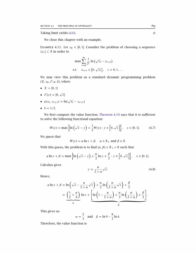
SECTION 4.3 THE PRINCIPLE OF OPTIMALITY 69
Taking limit yields (4.6). ut
We close this chapter with an example.
Example 4.11. Let x0 2 Œ0; 1�. Consider the problem of choosing a sequence
fxtg � R in order to
max1XtD0
1
2tln�pxt � xtC1
�s.t. xtC1 2
�0;pxt�; t D 0; 1; : : :
We may view this problem as a standard dynamic programming problem
.X; x0; �; '; ı/, where
� X D Œ0; 1�
� � .x/ D Œ0;px�
� '.xt ; xtC1/ D ln.pxt � xtC1/
� ı D 1=2.
We first compute the value function. Theorem 4.10 says that it is sufficient
to solve the following functional equation:
W.x/ D max
�ln�p
x � y�C1
2W.y/ W y 2
h0;pxi�; x 2 Œ0; 1�: (4.7)
We guess that
W.x/ D ˛ ln x C ˇ; ˛ 2 RC and ˇ 2 R:
With this guess, the problem is to find .˛; ˇ/ 2 RC � R such that
˛ ln x C ˇ D max
�ln�p
x � y�C˛
2lny C
ˇ
2W y 2
h0;pxi�; x 2 Œ0; 1�:
Calculus gives
y D˛
2C ˛
px: (4.8)
Hence,
˛ ln x C ˇ D ln
�px �
˛
2C ˛
px
�C˛
2ln
�˛
2C ˛
px
�Cˇ
2
D
�1
2C˛
4
�™
˛
ln x C
"ln
�1 �
˛
2C ˛
�C˛
2ln
�˛
2C ˛
�Cˇ
2
#•
ˇ
:
This gives us
˛ D2
3and ˇ D ln 9 �
8
3ln 4:
Therefore, the value function is

70 CHAPTER 4 DYNAMIC OPTIMIZATION THEORY
0 x1
−4
−3
−2
−1
1
V.x/
P.x/
Figure 4.2. The value function V.x/ and the optimal policy correspon-dence P.x/.
V.x/ D2
3ln x C ln 9 �
8
3ln 4; x 2 Œ0; 1�:
Then let us consider the optimal policy correspondence, P.x/. We have the
following problem
max f'.x; y/C ıV .y/ W y 2 � .x/g ;
which gives
P.x/ D
�1
4
px
�; x 2 Œ0; 1�:
See Figure 4.2.

5METRIC SPACES
The ideas of “metric” and “metric space” are abstractions of the concept of
distance in Euclidean space. Most of the ideas about metric spaces in general
are motivated by geometric ideas about sets in R or Rn, where n > 1.
There are a lot of excellent introductory references for the analysis of met-
ric spaces, e.g., Kolmogorov and Fomin (1970), Apostol (1974), Rudin (1976),
Gamelin and Greene (1999, Chapter 1), Carothers (2000), Zorich (2004a), Shirali
and Vasudeva (2006), Ok (2007), etc. For more advanced references, Folland
(1999), Dudley (2002) and Royden and Fitzpatrick (2010) are classic texts.
This chapter is based on Carothers (2000, Part One) and Ok (2007, Chapter
C). Our discussion is very elementary and incomplete. Anyone wants to learn
metric spaces should refer a text from the above list.
5.1 Basic Notions
Given a set X ¤ ¿, our first order of business is to define a distance function
on X . Suppose X D R2. What would we want a “reasonable” distance to do?
Definition 5.1 (Metric). LetX be a nonempty set. A function d W X�X ! Œ0;1/
is called a metric provided for all x; y; z 2 X ,
a. d.x; y/ D 0 iff x D y;
b. (Symmetry) d.x; y/ D d.y; x/;
c. (Triangle Inequality) d.x; y/ 6 d.x; z/C d.z; y/.
If d is a metric on X , we say that .X; d/ is a metric space. If .X; d/ is a metric
space and Y is a subset of X , then the restriction d 0 of d to Y � Y is clearly a
metric on Y . The metric space .Y; d 0/ is called a subspace of .X; d/.1
I Exercise 5.2. Prove that d.x; y/ > 0 for all x; y 2 X by (a)—(c) in Defini-
tion 5.1.
1 Precisely, d 0 D d�.Y � Y /.
71

72 CHAPTER 5 METRIC SPACES
Remark 5.3. Sometimes we suppress mention of the metric d and refer to X
itself as being a metric space.
Example 5.4. (a) The real line R with the metric d.x; y/ D jx � yj is a metric
space. More generally, Rn is a metric space when provided with the metric
d�.x1; : : : ; xn/; .y1; : : : ; yn/
�D
pnXkD1
.xk � yk/2;
called the usual metric on Rn. The space .Rn; d / is called the n-dimensional
Euclidean space.
(b) Let X ¤ ¿. Then X admits at least one metric: the discrete metric d defined
by setting
d.x; y/ D
˚1 if x ¤ y
0 if x D y:
I Exercise 5.5. Prove that the functions defined in Example 5.4 are metrics.
5.2 Convergent Sequences
Open Balls
Our aim is to define and discuss the notions of convergence and continuity
in metric space. Before this, we need to introduce some notation for “small”
sets. Throughout this section, we will assume that we are always dealing with
a generic metric space .X; d/, unless otherwise specified.
Definition 5.6 (Open Ball). For a point x 2 X and r > 0, the set
B.xI r/´˚x0 2 X W d.x0; x/ < r
is called the open ball centered at x of radius r .
Example 5.7. In R we have B.xI r/ D .x � r; x C r/; in R2 the set B.xI r/ is the
open disk of radius r centered at x.
I Exercise 5.8. Consider the discrete metric space defined in Example 5.4(b).
Find B.xI 1/ and B.xI 2/, where x 2 X .
A subset A � X is bounded if there is x 2 X and r > 0 such that A � B.xI r/;
that is, A is bounded if it is contained in some ball of large enough radius. But
exactly which x and r does not much matter.

SECTION 5.2 CONVERGENT SEQUENCES 73
Convergence
In order to prove the existence of a vector satisfying a desired property, it
is common to establish an appropriate sequence of vectors converging to a
limit. In many cases the limit of this sequence can be shown to satisfy the
required property. It is for this reason that the concept of convergence plays an
important role in analysis. Thus, we have the convergence of sequences of real
numbers, the convergence of sequences of complex numbers, the convergence
of sequence of functions, etc.
We will use the following terminology to define convergence:
Definition 5.9 (Neighborhood). A neighborhood (nhood, for short) of x is any
set containing an open ball about x. Intuitively, you should think of a nhood
of x as a “thick” set of points near x.
We now discuss the convergence of sequences that live in metric space. Its
value will be made clear through seeing how often it will be called in subse-
quent work.
Definition 5.10 (Convergence). A sequence fxng is said to converge to the
point x 2 X if
limn!1
d.xn; x/ D 0:
In this case, x is the limit of fxng and we write xn ! x, or limn!1 xn D x.
Remark 5.11. Since the definition of convergence is stated in terms of the se-
quence of real numbers fd.xn; x/g, we can easily derive the following equivalent
reformulations:
xn ! x iff, given any " > 0, there is an N 2 N
such that d.xn; x/ < " whenever n > N ,(C1)
or
xn ! x iff, given any " > 0, there is an N 2 N
such that fxn W n > N g � B.xI "/.(C2)
If it should happen that fxn W n > N g � A for some N 2 N, we say that the
sequence fxng is eventually in A. Thus, our last formulation (C2) can be written
xn ! x iff, given any " > 0, the sequence fxng is eventually in B.xI "/; (C3)
or, in yet another incarnation,
xn ! x iff fxng is eventually in every nhood of x: (C4)
This final version (C4) is blessed by a total lack of N s and "s!
Lemma 5.12. The limit of a convergent sequence in a metric space is unique.

74 CHAPTER 5 METRIC SPACES
Proof. Suppose that x; y 2 X are both limits of a sequence fxng in X . Then for
all n,
d.x; y/ 6 d.x; xn/C d.xn; y/:
Let n ! 1. Then the RHS of the above display tends to 0, so that d.x; y/ D 0.
Consequently, x D y. ut
Example 5.13. (a) A sequence fxng is convergent in a discrete space iff it is
eventually constant.
(b) Take any n 2 N, and let fxmg D f.x1;m; : : : ; xn;m/g be a sequence in Rn. It is
easy to show that xm ! .x1; : : : ; xn/ iff xi;m ! xi for each i D 1; : : : ; n.
5.3 Open Sets and Closed Sets
Open Sets
We now make precise the vague notion of a “thick” set in a metric space: a
“thick” set is one that contains an entire nhood of each of its points. Let us
give it a better name: open set.
Definition 5.14 (Open Set). A subset U of X is said to be open provided for
every point x 2 U , there is an open ball centered at x that is contained in
U . In other words, U is open if, given x 2 U , there is some r > 0 such that
B.xI r/ � U .
Example 5.15. We show that an open ball is open. Take an arbitrary x0 2
B.xI r/ and define r 0 D r � d.x0; x/. Let y 2 B.x0I r 0/. Then d.y; x0/ < r 0, so
that, by the triangle inequality,
d.y; x/ 6 d.y; x0/C d.x0; x/ < r 0 C d.x0; x/ D r:
Therefore, B.x0I r 0/ � B.xI r/. See Figure 5.1.
Theorem 5.16. The open sets in a metric space .X; d/ have the following
properties:
a. Any union of open sets is open.
b. Any finite intersection of open sets is open.
c. ¿ and X are both open.
Proof. (a) Let fO�g�2� be a family of open subsets of X and let O DS�2�O�.
Suppose x 2 O . Then there exists an index � such that x 2 O�. Since O� is
open, there exists some r > 0 such that B.xI r/ � O�. Then B.xI r/ � O .

SECTION 5.3 OPEN SETS AND CLOSED SETS 75
x0 r 0
r
x
Figure 5.1. An open ball is open.
(b) Let O1; : : : ; Om be open subsets of X and let O D O1 \ � � �Om. Let y 2 O .
Since each Oi is open, there exists ri > 0 such that
B.yI ri / � Oi ; 8 i D 1; : : : ; m:
Set r D minfr1; : : : ; rmg.
(c) ¿ is open since ¿ has no elements and, obviously, X is open. ut
Remark 5.17. The finiteness assumption in Theorem 5.16(2) is essential. In R,
we have1\nD1
B.0I 1=n/ D f0g;
which is not open in R.
Closed Sets
Definition 5.18 (Closed Set). A set F in a metric space .X; d/ is said to be a
closed set if its complement X X F is open (see Definition 5.14).
All statements concerning open sets may be translated into statements con-
cerning closed sets.
I Exercise 5.19. Prove:
a. ¿ and X are closed.
b. An arbitrary intersection of closed sets is closed. A finite union of closed sets
is closed.

76 CHAPTER 5 METRIC SPACES
c. Any finite set is closed.
Observe that the Definition 5.18 depends on a knowledge of open sets. We
would like to define a closed set in terms of, say, sequences. First observe that
F is closed iff X X F is open, and so F is closed iff
x 2 X X F H) B.xI r/ � X X F for some r > 0:
But this is the same as saying: F is closed iff
B.xI r/ \ F ¤ ¿ for every r > 0 H) x 2 F: (5.1)
Remark 5.20. Intuitively, a point x that satisfies B.xI r/ \ F ¤ ¿ for every
r > 0 is evidently “very close” to F in the sense that x cannot be separated
from F by any positive distance. At worst, x might be on the “boundary” of
F . Thus, condition (5.1) is telling us that a set is closed iff it contains all such
“boundary” points.
Let us now translate condition (5.1) into a sequential characterization of
closed sets.
Theorem 5.21. Given a set F in .X; d/, the following are equivalent:
a. F is closed; that is, X X F is open.
b. If B.xI r/ \ F ¤ ¿ for every r > 0, then x 2 F .
c. If a sequence fxng � F converges to some point x 2 X , then x 2 F .
Proof. (a () b) This is clear from our observations above and the definition
of an open set.
(b H) c) Suppose that fxng � F and xn ! x 2 X . Then B.xI r/ contains
infinitely many xn for any r > 0, and hence B.xI r/\F ¤ ¿ for any r > 0. Thus
x 2 F , by (b).
(c H) b) If B.xI r/ \ F ¤ ¿ for all r > 0, then for each n there is an xn 2
B.xI 1=n/. The sequence fxng satisfies fxng � F and xn ! x. Hence, by (c),
x 2 F . ut
Interior and Closure
Sets are not “doors”! For example, X is open and closed, but .0; 1� is neither
open nor closed in R. However, it is possible to describe the “open part” of a
set and the “closure” of a set.

SECTION 5.4 CONTINUOUS FUNCTIONS 77
Definition 5.22 (Interior). Given a set E in .X; d/, we define the interior of E,
written EB, to be the largest open set contained in E. That is,
EB D[˚
U W U is open and U � E
D
[˚B.xI r/ W B.xI r/ � E and for some x 2 E; r > 0
D˚x 2 E W B.xI r/ � E for some r > 0
:
Definition 5.23 (Closure). For a subset E of a metric space X , the closure of
E, written xE, is the smallest closed set containing E. That is,
xE D\˚
F W F is closed and E � F:
Clearly, EB is an open subset of E and xE is a closed set containing E.
You will need the following result in Mas-Colell, Whinston and Green (1995).
Lemma 5.24. If A is convex, then so is xA.
Proof. Take arbitrary points x;y 2 xA. We need to show that Œx;y� � xA. Let
x 2 Œx;y�, so z D �x C .1 � �/y for some � 2 Œ0; 1�. There exist sequences
fxng � A and fyng � A such that xn ! x and yn ! y . Since A is convex, we
have zn´ �xnC .1��/yn 2 A for all n 2 N. Therefore, zn ! �xC .1��/y D z,
so z 2 xA. ut
I Exercise 5.25. Show that if A � B , then xA � xB .
5.4 Continuous Functions
Throughout this section, unless otherwise specified, .X; dX / and .Y; dY / are
arbitrary metric spaces.
Definition 5.26 (Continuous Mapping). We say that the map f W X ! Y is
continuous at a point x 2 X if, for any " > 0, there exists a ı > 0 (which may
depend on f , x and ") such that for each y 2 Y (see Figure 5.2)
dX .x; y/ < ı implies dY�f .x/; f .y/
�< ":
Put differently, f is continuous at x if, for any " > 0, there exists a ı > 0 such
that
f�BX .xI ı/
�� BY .f .x/I "/:
If f is continuous at every point of X , we simply say that f is continuous on
X , or often just that f is continuous.
We now turn to characterize continuity in terms of open sets, closed sets
and sequences.

78 CHAPTER 5 METRIC SPACES
xf .x/
y
f .y/
ı
"
Figure 5.2. Inequalities in Definition 5.26 illustrated in the case of Eu-clidean planes X D R2 and Y D R2.
Theorem 5.27. Given f W X ! Y , the following are equivalent:
a. f is continuous on X (by the "-ı definition).
b. For every x 2 X , if xn ! x in X , then f .xn/! f .x/ in Y .
c. If E is closed in Y , then f �1.E/ is closed in X .
d. If V is open in Y , then f �1.V / is open in X .
Proof. (a H) b) Suppose that xn ! x 2 X . Given " > 0, let ı > 0 be such
that f .BX .xI ı// � BY .f .x/I "/. Since fxng is eventually in BX .xI ı/, the sequence
ff .xn/g is eventually in BY .f .x/I "/. Since " is arbitrary, this means that f .xn/!
f .x/ 2 Y .
(b H) c) Let E � Y be closed. To show f �1.E/ � X is closed, we only need
to show that for every convergent sequence fxng � f �1.E/ with xn ! x, we
have x 2 f �1.E/. Observe that fxng � f �1.E/ implies that ff .xn/g � E. It
follows from (b) that f .xn/! f .x/. Since E is closed, we have f .x/ 2 E and so
x 2 f �1.E/.
(c () d) It is evident since for every set A � Y we have f �1.Y X A/ D
X X f �1.A/.
(d H) a) Given x 2 X and " > 0, the set BY .f .x/I "/ is open in Y and so, by (d),
the set f �1.BY .f .x/I "// is open in X . But then there exists some ı > 0 such
that BX .xI ı/ � f �1.BY .f .x/I "// since x 2 f �1.BY .f .x/I "//. ut
Example 5.28. Let f W X ! R is a continuous real-valued function. Then the
set E ´ fx 2 X W f .x/ D 0g is closed.

SECTION 5.5 COMPLETE METRIC SPACES 79
5.5 Complete Metric Spaces
Definition 5.29 (Cauchy Sequence). A sequence fxng in a metric space .X; d/
is said to be a Cauchy sequence if for every " > 0, there exists an M 2 N (which
may depend on ") such that d.xk ; x`/ < " for all k; ` >M .
Metric spaces in which every Cauchy sequence is convergent are of partic-
ular interest in analysis; in such spaces it is possible to identify convergent
sequences without explicitly identifying their limits.
Example 5.30. (a) The sequence f1=ng is a Cauchy sequence in R becauseˇ̌̌̌1
k�1
`
ˇ̌̌̌6ˇ̌̌̌1
k
ˇ̌̌̌C
ˇ̌̌̌1
`
ˇ̌̌̌! 0 as k; `!1:
(b) Every convergent sequence fxng � X is Cauchy (Prove it). A Cauchy se-
quence need not converge. For example, f1=ng is Cauchy in .0; 1�, but it does
not converge in .0; 1� since 1=n! 0 … .0; 1�.
Remark 5.31. The difference between the definition of convergence (Defini-
tion 5.10) and the definition of a Cauchy sequence is that the limit is explicitly
involved in the former, but not in the latter.
Definition 5.32 (Completeness). A metric space X is said to be complete if
every Cauchy sequence in X converges to a point in X .
Example 5.33. All Euclidean n-spaces are complete. One should remember this
important fact though we are not going to prove it.2
Recall that .0; 1� is not a complete metric subspace of R, while Œ0; 1� is. This
suggests a tight connection between the closedness of a set and its complete-
ness as a metric subspace.
Proposition 5.34. Let X be a metric space, and Y a metric subspace of X .
If Y is complete, then it is closed in X . Conversely, if Y is closed in X and X
is complete, then Y is complete.
Proof. (i) Let Y be complete, and take an arbitrary fxng � Y that converges
in X . Then fxng is Cauchy, and thus lim xn 2 Y . It follows from Theorem 5.21
that Y is closed.
(ii) Suppose that X is complete and Y is closed in X . If fxng is a Cauchy se-
quence in Y , then it is Cauchy in X . So xn ! x 2 X . But since Y is closed, it
must be the case that x 2 Y (Theorem 5.21). It follows that Y is complete. ut
2 The proof can be found in Rudin (1976, Theorem 3.11).

80 CHAPTER 5 METRIC SPACES
5.6 Compact Metric Spaces
A compact space is the best of all possible worlds. Compactness is one of the
most fundamental concepts of real analysis and one that plays an important
role in optimization theory.
Definition 5.35 (Open Cover). Let X be a metric space and S � X . A class O
of subsets of X is said to cover S if S �S
O. If all members of such a class O
are open in X , then we say that O is an open cover of S .
Definition 5.36 (Compactness). A metric space X is said to be compact if
every open cover of X has a finite subset that also covers X . A subset S of X
is said to be compact in X (or a compact subset of X ) if every open cover of S
has a finite subset that also covers S .
Example 5.37. We claim that .0; 1/ is not compact in R. Consider the collection
O ´ f.1=n; 1/ W n D 1; 2; : : :g and observe that .0; 1/ D .1=2; 1/ [ .1=3; 1/ [ � � � ,
that is, O is an open cover of .0; 1/. However, O does not have a finite subset
covering .0; 1/.
Theorem 5.38 (Characterization of Compactness for a Metric Space). For
a metric space X , the following three assertions are equivalent:
a. X is complete and totally bounded;
b. X is compact;
c. X is sequentially compact.
Proof. See Royden and Fitzpatrick (2010, Section 9.5). ut

References
[1] Aliprantis, Charalambos D. and Kim C. Border (2006) Infinite Dimen-
sional Analysis: A Hitchhiker’s Guide, Berlin: Springer-Verlag, 3rd edition.
[61]
[2] Apostol, Tom M. (1967) Calculus, Volume I: One-Variable Calculus, with
an Introduction to Linear Algebra, New York: John Wiley & Sons, Inc. [41]
[3] (1974) Mathematical Analysis: Pearson Education, 2nd edition.
[71]
[4] Aubin, Jean-Pierre and Hélène Frankowska (1990) Set-Valued Analy-
sis, Boston: Birkhäuser. [61]
[5] Berkovitz, Leonard D. (2002) Convexity and Optimization in Rn, Pure
and Applied Mathematics: A Wiley-Interscience Series of Texts, Mono-
graphs and Tracts, New York: Wiley-Interscience. [45, 51]
[6] Carothers, N. L. (2000) Real Analysis, Cambridge, Massachusetts: Cam-
bridge University Press. [71]
[7] Crossley, Martin D. (2005) Essential Topology, Springer Undergraduate
Mathematics Series, London: Springer-Verlag. [5]
[8] Dudley, Richard Mansfield (2002) Real Analysis and Probability, 74
of Cambridge Studies in Advanced Mathematics, New York: Cambridge
University Press, 2nd edition. [71]
[9] Duffie, Darrell (2001) Dynamic Asset Pricing Theory, New Jersey:
Princeton University Press, 3rd edition. [61]
[10] Duggan, John (2010) “Notes on Optimization and Pareto Optimality,”
Rochester University, http://www.johnduggan.net/lecture[23, 27, 40]
[11] Folland, Gerald B (1999) Real Analysis: Modern Techniques and Their
Applications, Pure and Applied Mathematics: A Wiley-Interscience Series
of Texts, Monographs and Tracts, New York: John Wiley & Sons, Inc. 2nd
edition. [71]
81

82 REFERENCES
[12] Gamelin, Theodore W. and Robert Everist Greene (1999) Introduc-
tion to Topology, New York: Dover Publications, Inc. 2nd edition. [71]
[13] Jehle, Geoffrey A. and Philip J. Reny (2011) Advanced Microeconomic
Theory, New York: Prentice Hall, 3rd edition. [23, 34, 51]
[14] Kolmogorov, A. N. and S. V. Fomin (1970) Introductory Real Analysis,
New York: Dover Publications, Inc. [71]
[15] Ljungqvist, Lars and Thomas J. Sargent (2004) Recursive Macroeco-
nomic Theory, Cambridge, Massachusetts: MIT Press, 2nd edition. [61]
[16] Luenberger, David G. (1969) Optimization by Vector Space Methods,
New York: John Wiley & Sons, Inc. [23, 45, 47]
[17] Mailath, George J. and Larry Samuelson (2006) Repeated Games and
Reputations: Long-Run Relationships, New York: Oxford University Press.
[61]
[18] Mas-Colell, Andreu, Michael D. Whinston, and Jerry R. Green
(1995) Microeconomic Theory, New York: Oxford University Press. [23,
53, 77]
[19] Milgrom, Paul (2004) Putting Auction Theory to Work, Cambridge, U.K.:
Cambridge University Press. [44]
[20] Milgrom, Paul and Ilya Segal (2002) “Envelope Theorems for Arbi-
trary Choice Sets,” Econometrica, 70 (2), pp. 583–601. [44]
[21] Munkres, James R. (1991) Analysis on Manifolds, Boulder, Colorado:
Westview Press. [1, 18, 20]
[22] Ok, Efe A. (2007) Real Analysis with Economic Applications, New Jersey:
Princeton University Press. [45, 61, 71]
[23] Rockafellar, R. Tyrrell (1970) Convex Analysis, Princeton Mathemati-
cal Series, New Jersey: Princeton University Press, 2nd edition. [45]
[24] Royden, Halsey and Patrick Fitzpatrick (2010) Real Analysis, New
Jersey: Prentice Hall, 4th edition. [45, 71, 80]
[25] Rudin, Walter (1976) Principles of Mathematical Analysis, New York:
McGraw-Hill Companies, Inc. 3rd edition. [16, 17, 18, 20, 71, 79]
[26] Shastri, Anant R. (2011) Elements of Differential Topology, Boca Raton,
FL: CRC Press. [30]
[27] Shirali, Satish and Harkrishan L. Vasudeva (2006) Metric Spaces,
London: Springer-Verlag. [71]
REFERENCES 83
[28] Spivak, Michael (1965) Calculus on Manifolds: A Modern Approach to
Classical Theorems of Advanced Calculus, Boulder, Colorado: Westview
Press. [1, 18, 20]
[29] Stokey, Nancy L. and Robert E. Lucas (1989) Recursive Methods in Eco-
nomic Dynamics, Cambridge, Massachusetts: Harvard University Press.
[61]
[30] Sundaram, Rangarajan K. (1996) A First Course in Optimization The-
ory, Cambridge, Massachusetts: Cambridge University Press. [23, 26, 27,
32, 34, 36, 57]
[31] Willard, Stephen (2004) General Topology, New York: Dover Publica-
tions, Inc. [4]
[32] Zorich, Vladimir A. (2004a) Mathematical Analysis I, Universitext,
Berlin: Springer-Verlag. [71]
[33] (2004b) Mathematical Analysis II, Universitext, Berlin: Springer-
Verlag. [41]


Index
C1, 16C1, 17Cr , 17n-dimensional Euclidean space, 72
Affine manifold, 47
Binding constraint, 34
Cauchy sequence, 79Chain Rule, 17Closed set, 75Closure, 77Cobb-Douglas function, 22compact set, 80Complete metric spaces, 79complete space, 79Component function, 5Concave function, 51Constraint qualification, 27, 36continuous function, 77continuous mapping, 77Continuously differentiable, 16Convex combination, 46Convex function, 51Convex hull, 47Convex set, 45Critical point, 25
Directional derivative, 8discrete metric, 72
Envelope, 41Epigraph, 52Euclidean n-space, 1
Half space, 48Hessian, 17Hyperplane, 47
Implicit function theorem, 20Inequality constrained optimization, 34Inferior set, 52Inner product, 2Interior, 4, 77interior, 77
Jacobian matrix, 13Jensen’s inequality, 54
Kuhn-Tucker Multipliers, 37Kuhn-Tucker Theorem, 36
Lagrange multipliers, 30Lagrange’s Method, 31Lagrange’s Theorem, 27Lagrangian, 31Level set, 14Limit, 5limit, 73
Maximizer, 25metric, 71metric space, 71
Negative definite, 18Negative semidefinite, 18neighborhood, 73Norm, 2
open ball, 72open cover, 80open set, 74Optimal path, 67Optimal policy correspondence, 67
Partial derivative, 11Positive definite, 18Positive semidefinite, 18
85

86 INDEX
Quadratic form, 18quasi-concave function, 51quasi-convex function, 51
Recursive method, 65
Second-order partial derivative, 17Separation theorem, 48Sequence, 5Slack constraint, 34Slater’s condition, 57
Standard dynamic programming problem,64
Strictly concave function, 51Strictly convex function, 51Strictly quasi-concave function, 51Strictly quasi-convex function, 51Subgraph, 52Superior set, 52
Unconstrained optimization, 25
Value function, 41, 43, 65