mathematics for physicists lea solutions
TRANSCRIPT
Chapter 1: Describing the universe
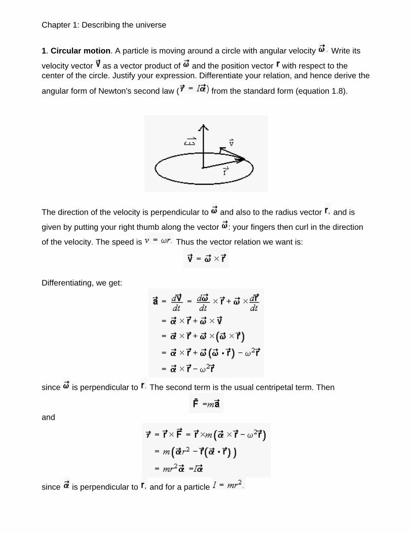
1. Circular motion. A particle is moving around a circle with angular velocity Write its
velocity vector as a vector product of and the position vector with respect to the center of the circle. Justify your expression. Differentiate your relation, and hence derive the
angular form of Newton's second law ( from the standard form (equation 1.8).
The direction of the velocity is perpendicular to and also to the radius vector and is
given by putting your right thumb along the vector : your fingers then curl in the direction
of the velocity. The speed is Thus the vector relation we want is:
Differentiating, we get:
since is perpendicular to The second term is the usual centripetal term. Then
and
since is perpendicular to and for a particle
2. Find two vectors, each perpendicular to the vector and perpendicular to each
other. Hint: Use dot and cross products. Determine the transformation matrix that allows
you to transform to a new coordinate system with axis along and and axes along your other two vectors.
We can find a vector perpendicular to by requiring that A vector satsifying this is:
Now to find the third vector we choose
To find the transformation matrix, first we find the magnitude of each vector and the corresponding unit vectors:
and
The elements of the transformation matrix are given by the dot products of the unit vectors along the old and new axes (equation 1.21)
To check, we evaluate:
as required. Similarly
and finally:
3. Show that the vectors (15, 12, 16), (-20, 9, 12) and (0,-4, 3) are mutually orthogonal and right handed. Determine the transformation matrix that transforms from the
original cordinate system, to a system with axis along axis along and
axis along Apply the transformation to find components of the vectors
and in the prime system. Discuss the result for vector
Two vectors are orthogonal if their dot product is zero.
and
Finally
So the vectors are mutually orthogonal. In addition
So the vectors form a right-handed set.
To find the transformation matrix, first we find the magnitude of each vector and the corresponding unit vectors.
So
Similarly
and
The elements of the transformation matrix are given by the dot products of the unit vectors along the old and new axes (equation 1.21)
Thus the matrix is:
Check:
as required.
Then:
and
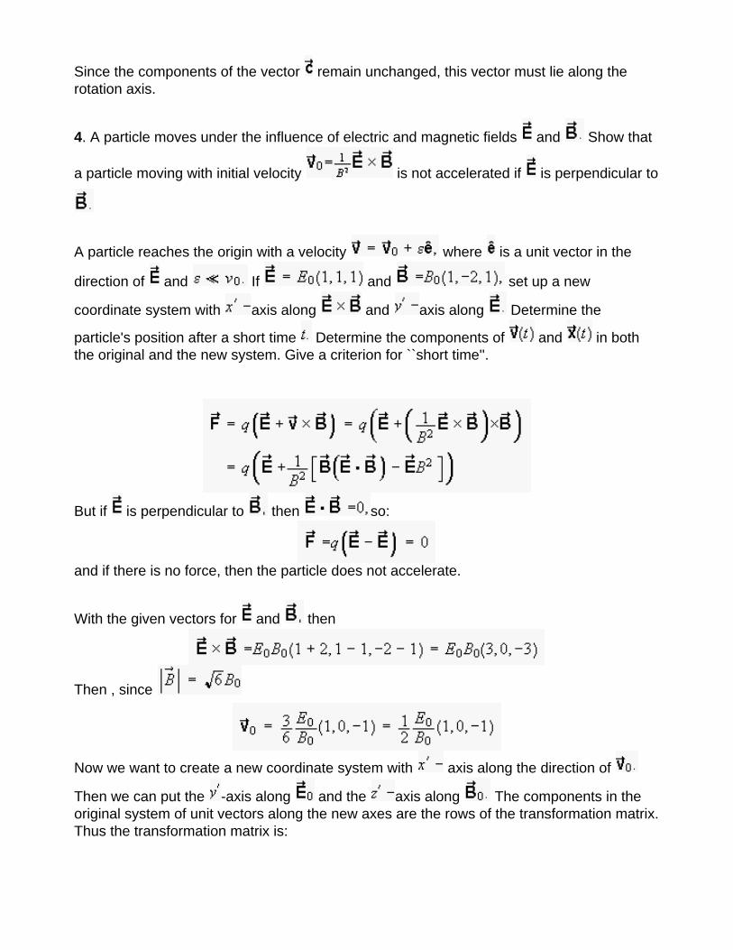
Since the components of the vector remain unchanged, this vector must lie along the rotation axis.
4. A particle moves under the influence of electric and magnetic fields and Show that
a particle moving with initial velocity is not accelerated if is perpendicular to
A particle reaches the origin with a velocity where is a unit vector in the
direction of and If and set up a new
coordinate system with axis along and axis along Determine the
particle's position after a short time Determine the components of and in both the original and the new system. Give a criterion for ``short time''.
But if is perpendicular to then so:
and if there is no force, then the particle does not accelerate.
With the given vectors for and then
Then , since
Now we want to create a new coordinate system with axis along the direction of
Then we can put the -axis along and the axis along The components in the original system of unit vectors along the new axes are the rows of the transformation matrix. Thus the transformation matrix is:
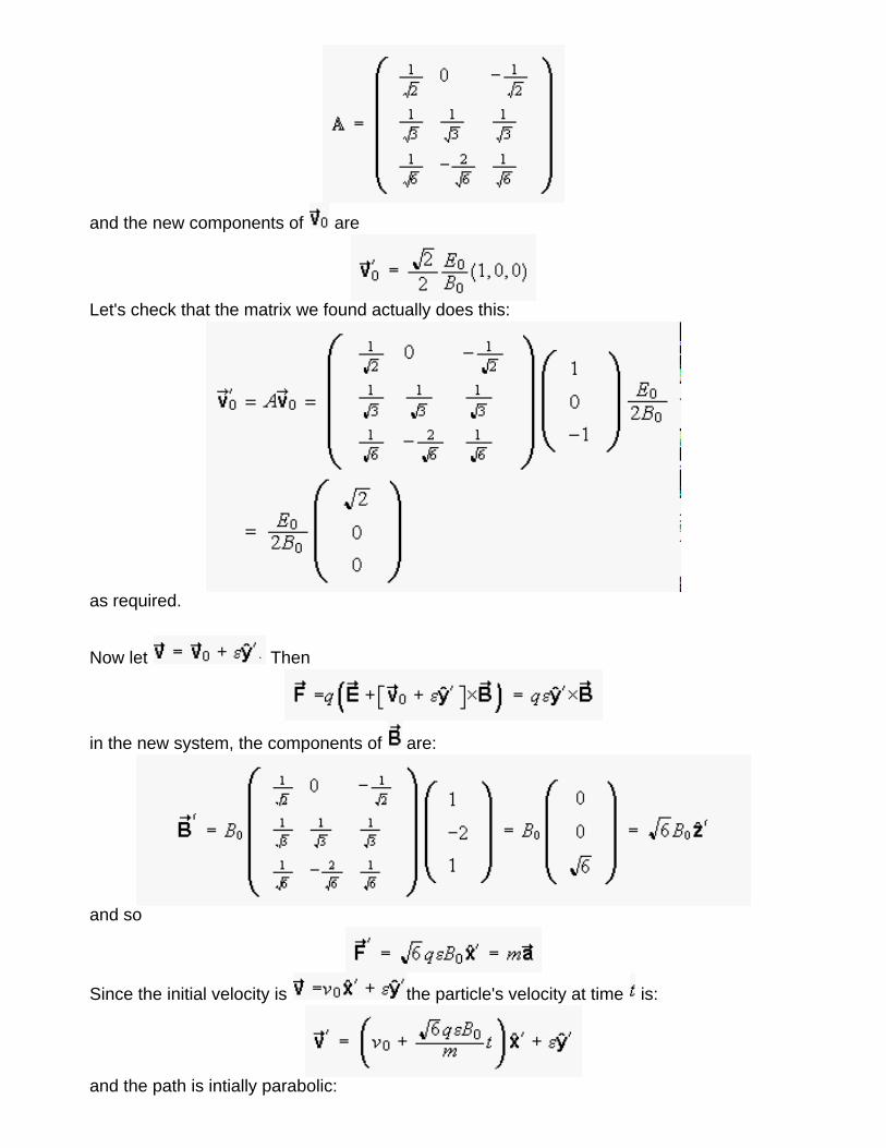
and the new components of are
Let's check that the matrix we found actually does this:
as required.
Now let Then
in the new system, the components of are:
and so
Since the initial velocity is the particle's velocity at time is:
and the path is intially parabolic:
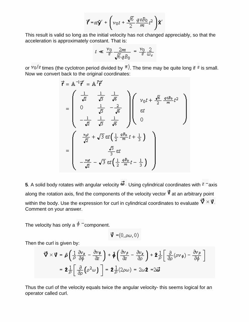
This result is valid so long as the initial velocity has not changed appreciably, so that the acceleration is approximately constant. That is:
or times (the cyclotron period divided by . The time may be quite long if is small. Now we convert back to the original coordinates:
5. A solid body rotates with angular velocity Using cylindrical coordinates with axis
along the rotation axis, find the components of the velocity vector at an arbitrary point
within the body. Use the expression for curl in cylindrical coordinates to evaluate Comment on your answer.
The velocity has only a component.
Then the curl is given by:
Thus the curl of the velocity equals twice the angular velocity- this seems logical for an operator called curl.
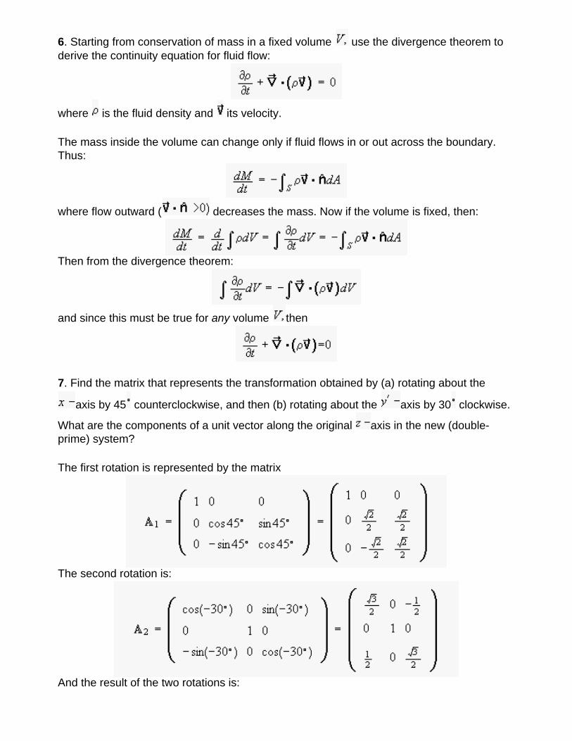
6. Starting from conservation of mass in a fixed volume use the divergence theorem to derive the continuity equation for fluid flow:
where is the fluid density and its velocity.
The mass inside the volume can change only if fluid flows in or out across the boundary. Thus:
where flow outward ( decreases the mass. Now if the volume is fixed, then:
Then from the divergence theorem:
and since this must be true for any volume then
7. Find the matrix that represents the transformation obtained by (a) rotating about the
axis by 45 counterclockwise, and then (b) rotating about the axis by 30 clockwise.
What are the components of a unit vector along the original axis in the new (double-prime) system?
The first rotation is represented by the matrix
The second rotation is:
And the result of the two rotations is:
The new components of the orignal axis are:
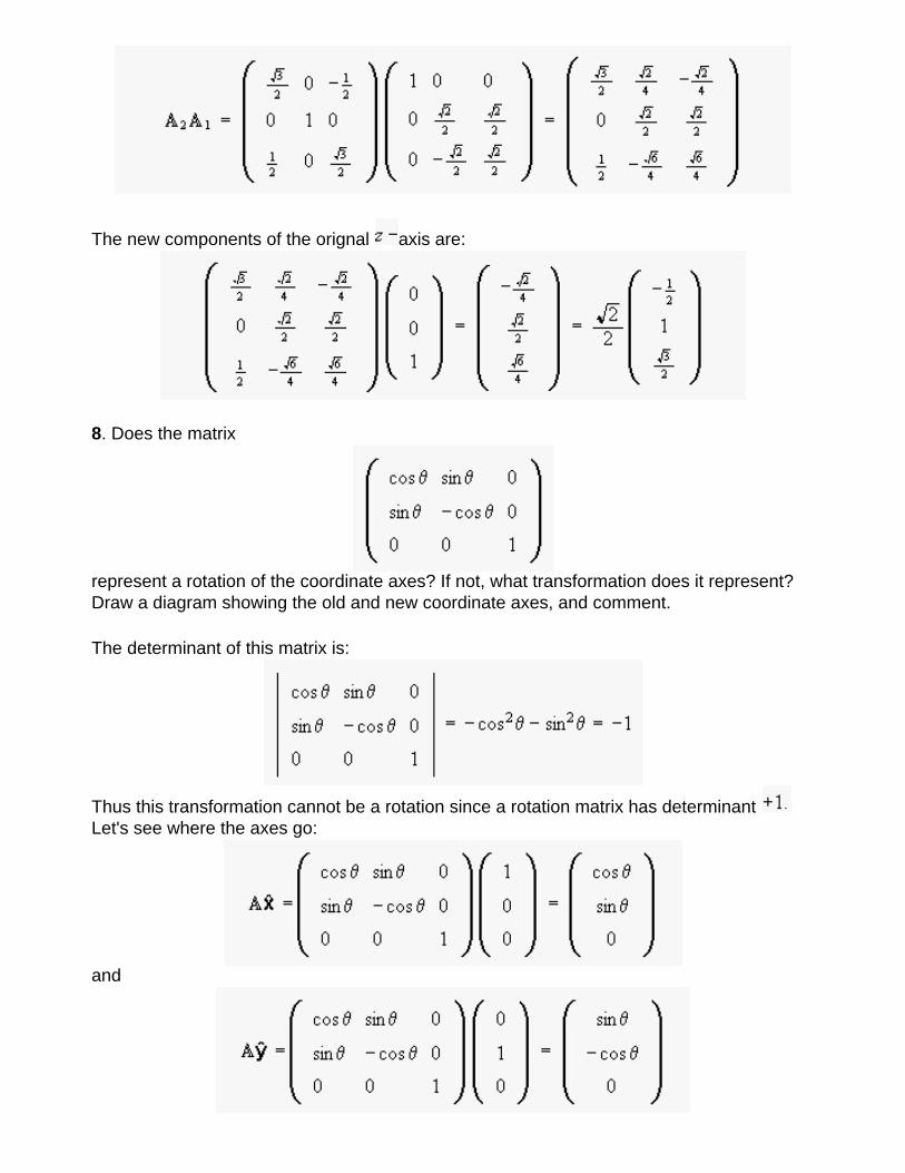
8. Does the matrix
represent a rotation of the coordinate axes? If not, what transformation does it represent? Draw a diagram showing the old and new coordinate axes, and comment.
The determinant of this matrix is:
Thus this transformation cannot be a rotation since a rotation matrix has determinant Let's see where the axes go:
and
while
These are the components of the original and axes in the new system. The new
and axes have the following components in the original system:
where
Thus:
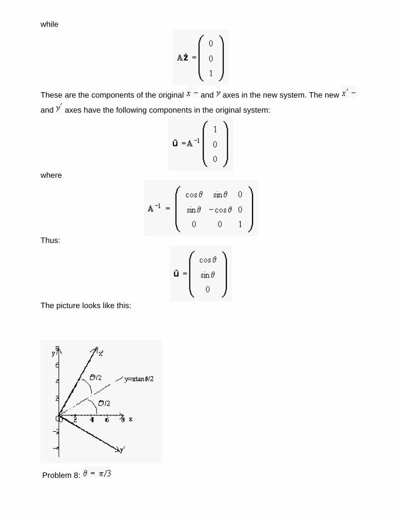
The picture looks like this:
Problem 8:
The matrix represents a reflection of the and axes about the line
9. Represent the following transformation using a matrix: (a) a rotation about the axis
through an angle followed by (b) a reflection in the line through the origin and in the
-plane, at an angle 2 to the original axis, where both angles are measured
counter-clockwise from the positive axis. Express your answer as a single matrix. You
should be able to recognize the matrix either as a rotation about the axis through an
angle or as a reflection in a line through the origin at an angle to the axis. Decide
whether this transformation is a reflection or a rotation, and give the value of (Note: For
the purposes of this problem, reflection in a line in the plane leaves the axis unchanged.)
Since only the and components are transformed, we may work with matrices. The rotation matrix is:
The line in which we reflect is at 2 to the original axis and thus at to the new
axis. Thus the matrix we want is (see Problem 8 above):
Thus the complete transformation is described by the matrix:
The determinant of this matrix is , and so the transformation is a reflection. It sends to
and to so it is a reflection in the axis (
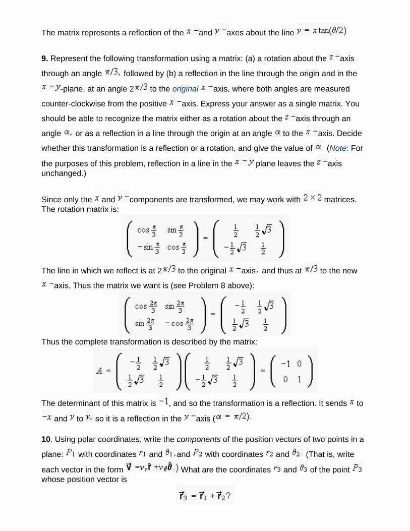
10. Using polar coordinates, write the components of the position vectors of two points in a
plane: with coordinates and and with coordinates and (That is, write
each vector in the form What are the coordinates and of the point whose position vector is
Hint: Start by drawing the position vectors.
Problem 10
The position vector has only a single component: the component. Thus the vectors are:
and
The sum also only has a single component:
where, from the diagram , and:
Thus has coordinates
where
and thus
We can check this in the special case Then
as required.
This document created by Scientific WorkPlace 4.1.
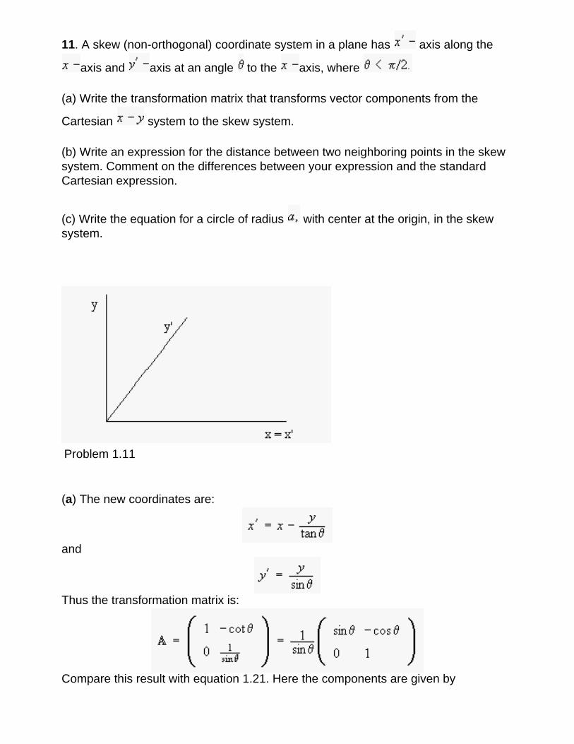
11. A skew (non-orthogonal) coordinate system in a plane has axis along the
axis and axis at an angle to the axis, where
(a) Write the transformation matrix that transforms vector components from the
Cartesian system to the skew system.
(b) Write an expression for the distance between two neighboring points in the skew system. Comment on the differences between your expression and the standard Cartesian expression.
(c) Write the equation for a circle of radius with center at the origin, in the skew system.
Problem 1.11
(a) The new coordinates are:
and
Thus the transformation matrix is:
Compare this result with equation 1.21. Here the components are given by
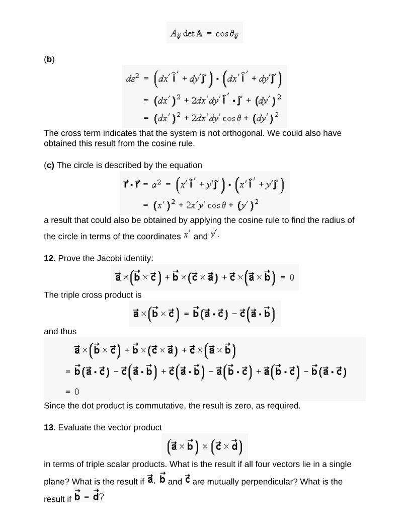
(b)
The cross term indicates that the system is not orthogonal. We could also have obtained this result from the cosine rule.
(c) The circle is described by the equation
a result that could also be obtained by applying the cosine rule to find the radius of
the circle in terms of the coordinates and
12. Prove the Jacobi identity:
The triple cross product is
and thus
Since the dot product is commutative, the result is zero, as required.
13. Evaluate the vector product
in terms of triple scalar products. What is the result if all four vectors lie in a single
plane? What is the result if and are mutually perpendicular? What is the
result if
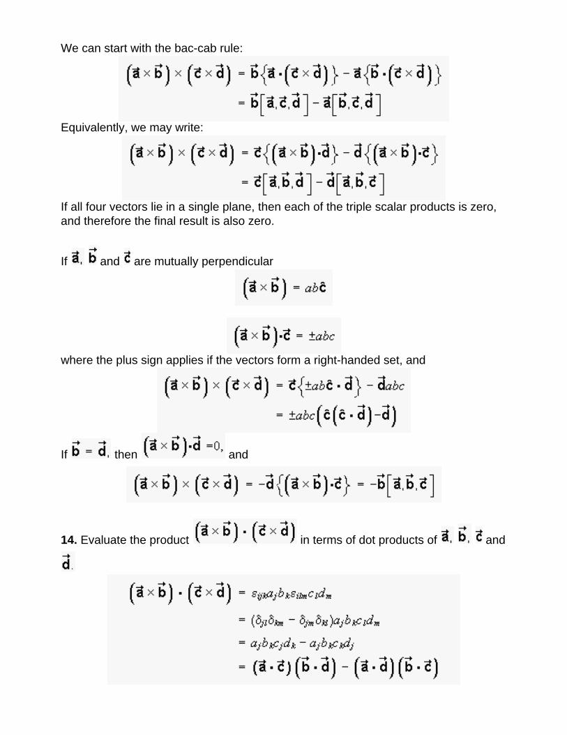
We can start with the bac-cab rule:
Equivalently, we may write:
If all four vectors lie in a single plane, then each of the triple scalar products is zero, and therefore the final result is also zero.
If and are mutually perpendicular
where the plus sign applies if the vectors form a right-handed set, and
If then and
14. Evaluate the product in terms of dot products of and
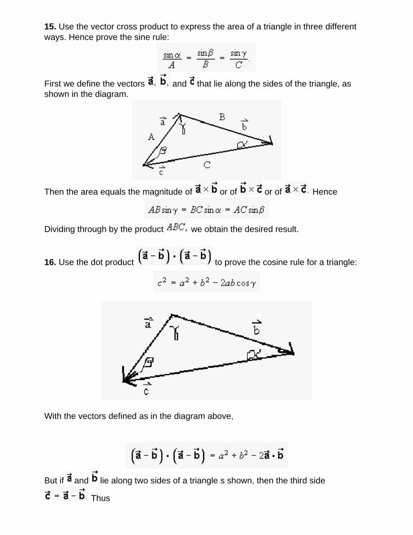
15. Use the vector cross product to express the area of a triangle in three different ways. Hence prove the sine rule:
First we define the vectors and that lie along the sides of the triangle, as shown in the diagram.
Then the area equals the magnitude of or of or of Hence
Dividing through by the product we obtain the desired result.
16. Use the dot product to prove the cosine rule for a triangle:
With the vectors defined as in the diagram above,
But if and lie along two sides of a triangle s shown, then the third side
Thus
as required.
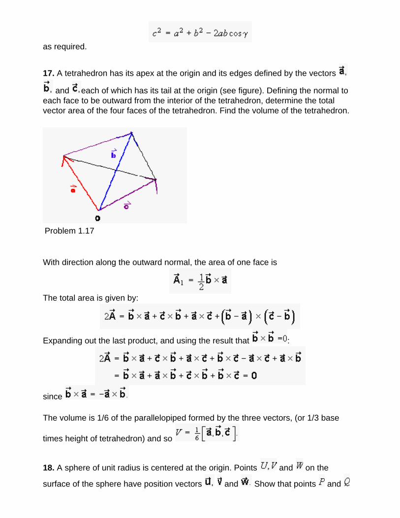
17. A tetrahedron has its apex at the origin and its edges defined by the vectors
and each of which has its tail at the origin (see figure). Defining the normal to each face to be outward from the interior of the tetrahedron, determine the total vector area of the four faces of the tetrahedron. Find the volume of the tetrahedron.
Problem 1.17
With direction along the outward normal, the area of one face is
The total area is given by:
Expanding out the last product, and using the result that :
since
The volume is 1/6 of the parallelopiped formed by the three vectors, (or 1/3 base
times height of tetrahedron) and so
18. A sphere of unit radius is centered at the origin. Points and on the
surface of the sphere have position vectors and Show that points and
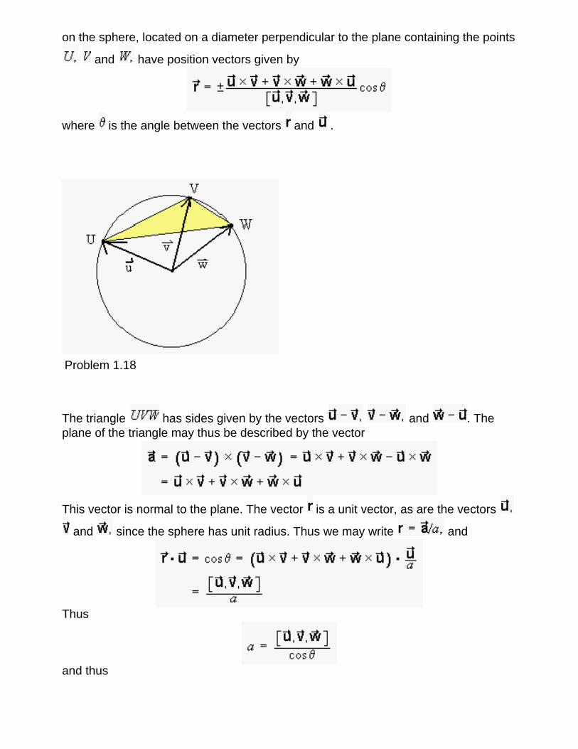
on the sphere, located on a diameter perpendicular to the plane containing the points
and have position vectors given by
where is the angle between the vectors and .
Problem 1.18
The triangle has sides given by the vectors and . The plane of the triangle may thus be described by the vector
This vector is normal to the plane. The vector is a unit vector, as are the vectors
and since the sphere has unit radius. Thus we may write and
Thus
and thus
To obtain both ends of the diameter, we need to add the sign, as given in the problem statement.
19. Show that
for any scalar field
because the order of the partial derivatives is irrelevant.
20. Find an expression for in terms of derivatives of and
Now remember that the differential operator operates on everything to its right, so, expanding the derivatives of the products, we have:
This document created by Scientific WorkPlace 4.1.
Chapter 1: Describing the universe
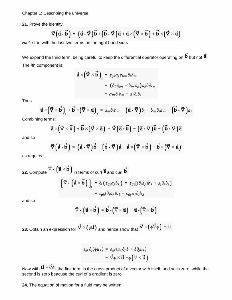
21. Prove the identity:
Hint: start with the last two terms on the right hand side.
We expand the third term, being careful to keep the differential operator operating on but not
The th component is:
Thus
Combining terms:
and so
as required.
22. Compute in terms of curl and curl
and so
23. Obtain an expression for and hence show that
Now with the first term is the cross product of a vector with itself, and so is zero, while the second is zero beacuse the curl of a gradient is zero.
24. The equation of motion for a fluid may be written
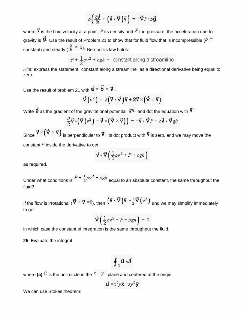
where is the fluid velocity at a point, its density and the pressure. the acceleration due to
gravity is Use the result of Problem 21 to show that for fluid flow that is incompressible (
constant) and steady ( Bernoulli's law holds:
Hint: express the statement ''constant along a streamline'' as a directional derivative being equal to zero.
Use the result of problem 21 with
Write as the gradient of the gravitational potential, and dot the equation with
Since is perpendicular to its dot product with is zero, and we may move the
constant inside the derivative to get:
as required.
Under what conditions is equal to an absolute constant, the same throughout the fluid?
If the flow is irrotational ( ), then and we may simplify immediately to get
in which case the constant of integration is the same throughout the fluid.
25. Evaluate the integral
where (a) is the unit circle in the plane and centered at the origin
We can use Stokes theorem:
Here the surface is in the plane, and the component of the curl is:
and so the integral is
(b) is a semicircle of radius with the flat side along the axis, the center of the circle at the origin, and
We need only the component of the curl.
and so the integral is zero.
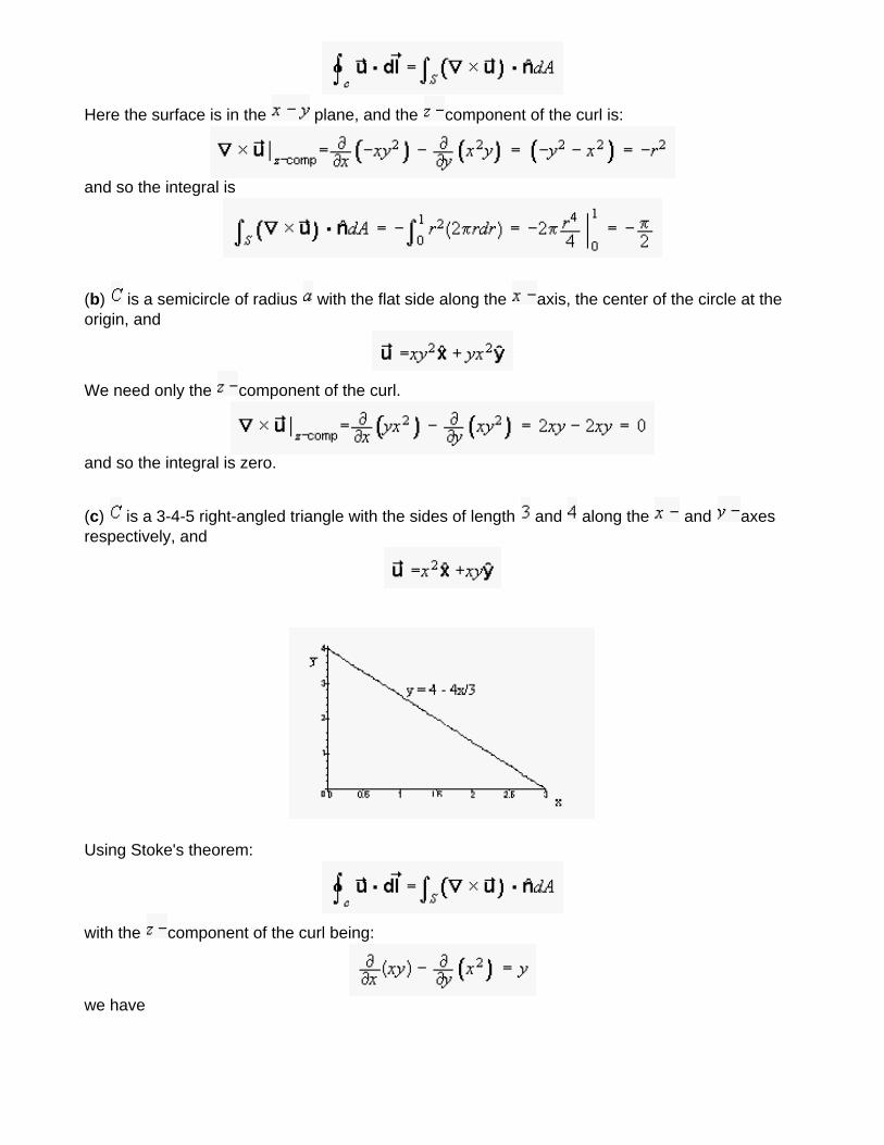
(c) is a 3-4-5 right-angled triangle with the sides of length and along the and axes respectively, and
Using Stoke's theorem:
with the component of the curl being:
we have
Or, doing the line integral:
The same result, as we expected, but the calculation is more difficult.
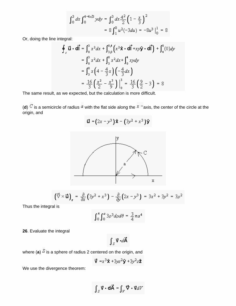
(d) is a semicircle of radius with the flat side along the axis, the center of the circle at the origin, and
Thus the integral is
26. Evaluate the integral
where (a) is a sphere of radius 2 centered on the origin, and
We use the divergence theorem:
Here
and so
(b) is a hemisphere of radius 1, with the center of the sphere at the origin, the flat side in the
plane, and
Integrating over the hemisphere, we get:
Doing the integral over first, the first term is zero, and we have:
27. Show that the vector
has zero divergence (it is solenoidal) and zero curl (it is irrotational). Find a scalar function such that
and a vector such that
and
and similarly for the other components.
If then Similarly, we obtain and
. Thus
will do the trick. The curl is a bit harder. We have:
Then:
from the first equation, and
from the second. Thus we can take and This gives
which also satisfies the last equation, and we are done:
28. Show that the vector
has zero divergence (it is solenoidal) and zero curl (it is irrotational) for . Find a scalar
function such that
and a vector such that
In spherical coordinates:
and
Then
and has only an component provided that , and is independent
of Then
is satisfied provided
satisfies all the constraints.
29. A surface is bounded by a curve The solid angle subtended by the surface at a point
where is in the vicinity of but not on the curve, is given by
Here is an element of area of the loop projected perpendicular to the vector is
the position vector of the point with respect to some chosen origin , and is a vector that labels an arbitrary point on the surface or the curve. Now let the curve be rigidly displaced by a
small amount . Express the resulting change in solid angle as an integral around the curve.
Hence show that
The solid angle subtended at P by an area element is
where is the element of surface area projected perpendicular to the vector from the origin to that element. The total change in solid angle due to the displacement of the loop is thus
and so
30. Prove the theorems (a)
We begin by proving the result for a differential cube. Start with the right hand side:
and since the result is true for one differential cube, and we can make up an arbitrary volume from
differential cubes as in the proof of the divergence theorem it is true in general.
b. We use the same method:
On the right hand side, the first pair of faces gives:
Including all the 6 sides we have:
and since the result is true for one differential cube, and we can make up an arbitrary volume from
differential cubes as in the proof of the divergence theorem it is true in general.
This document created by Scientific WorkPlace 4.1.
Chapter 1: Describing the universe
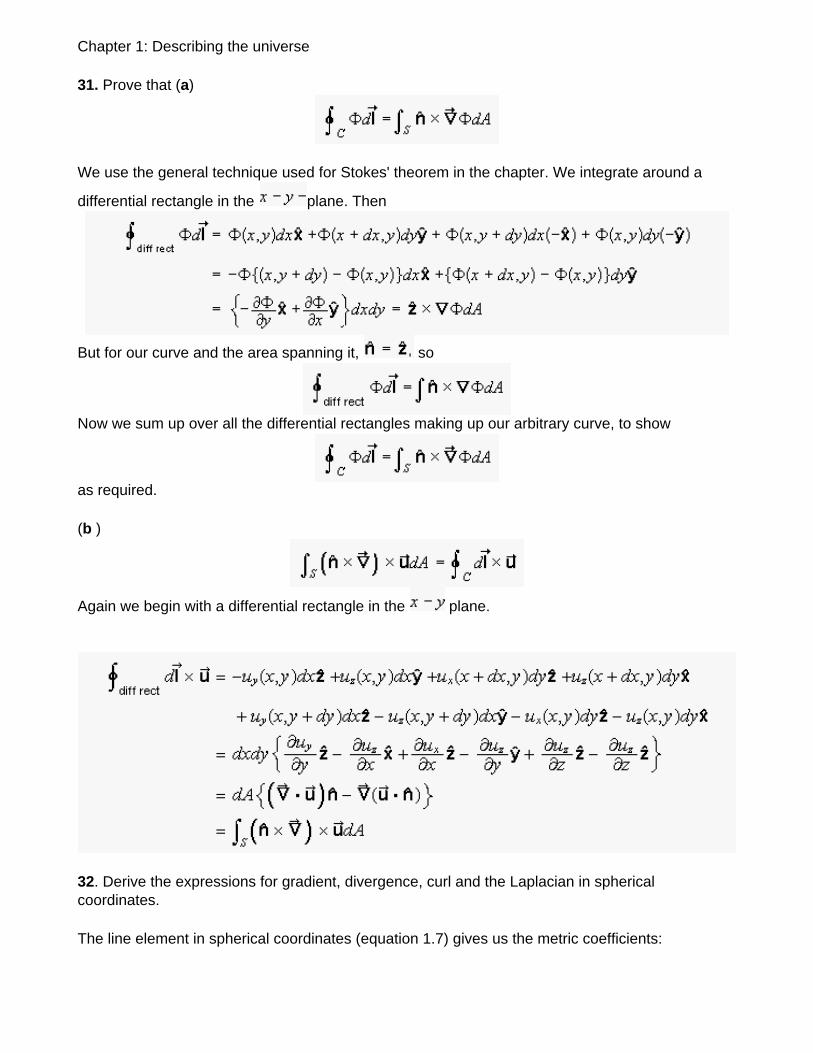
31. Prove that (a)
We use the general technique used for Stokes' theorem in the chapter. We integrate around a
differential rectangle in the plane. Then
But for our curve and the area spanning it, so
Now we sum up over all the differential rectangles making up our arbitrary curve, to show
as required.
(b )
Again we begin with a differential rectangle in the plane.
32. Derive the expressions for gradient, divergence, curl and the Laplacian in spherical coordinates.
The line element in spherical coordinates (equation 1.7) gives us the metric coefficients:
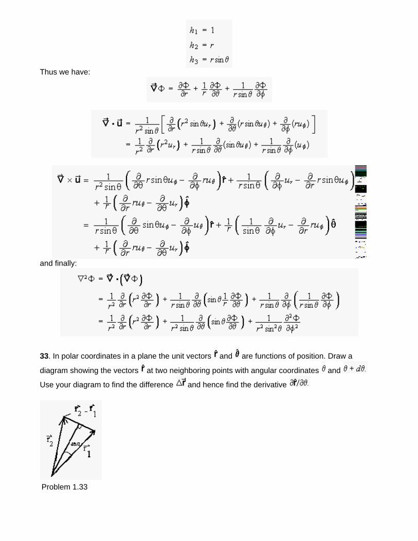
Thus we have:
and finally:
33. In polar coordinates in a plane the unit vectors and are functions of position. Draw a
diagram showing the vectors at two neighboring points with angular coordinates and
Use your diagram to find the difference and hence find the derivative
Problem 1.33
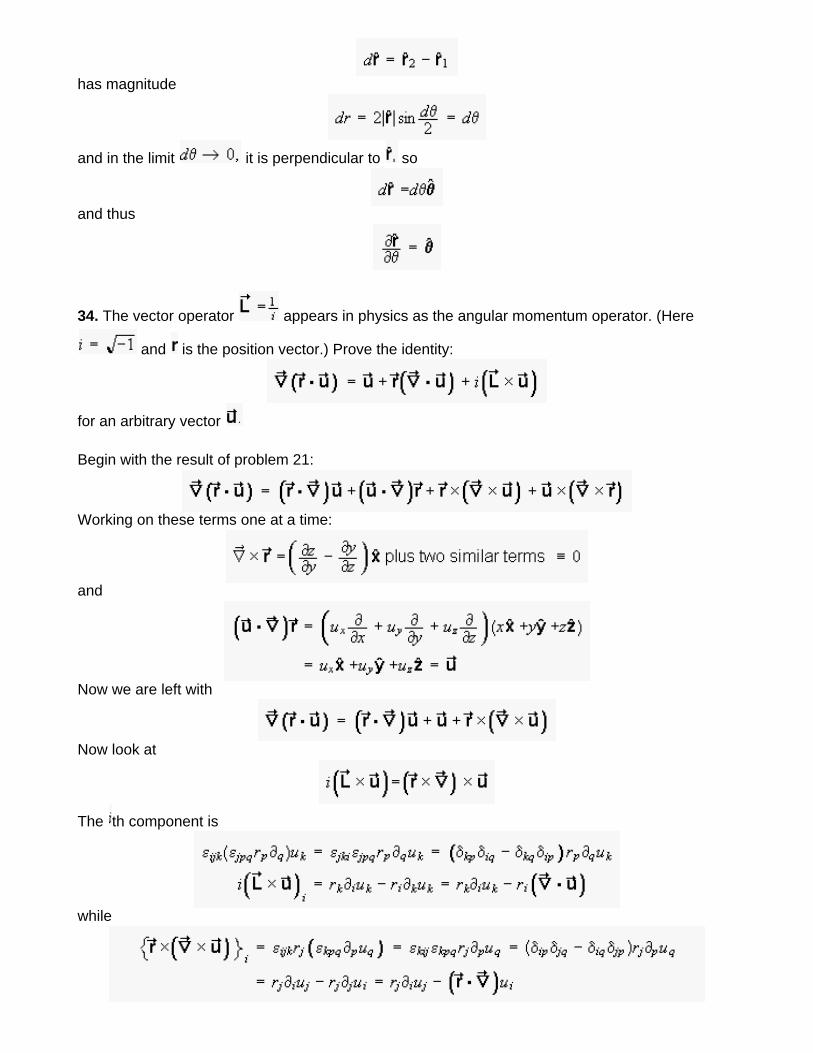
has magnitude
and in the limit it is perpendicular to so
and thus
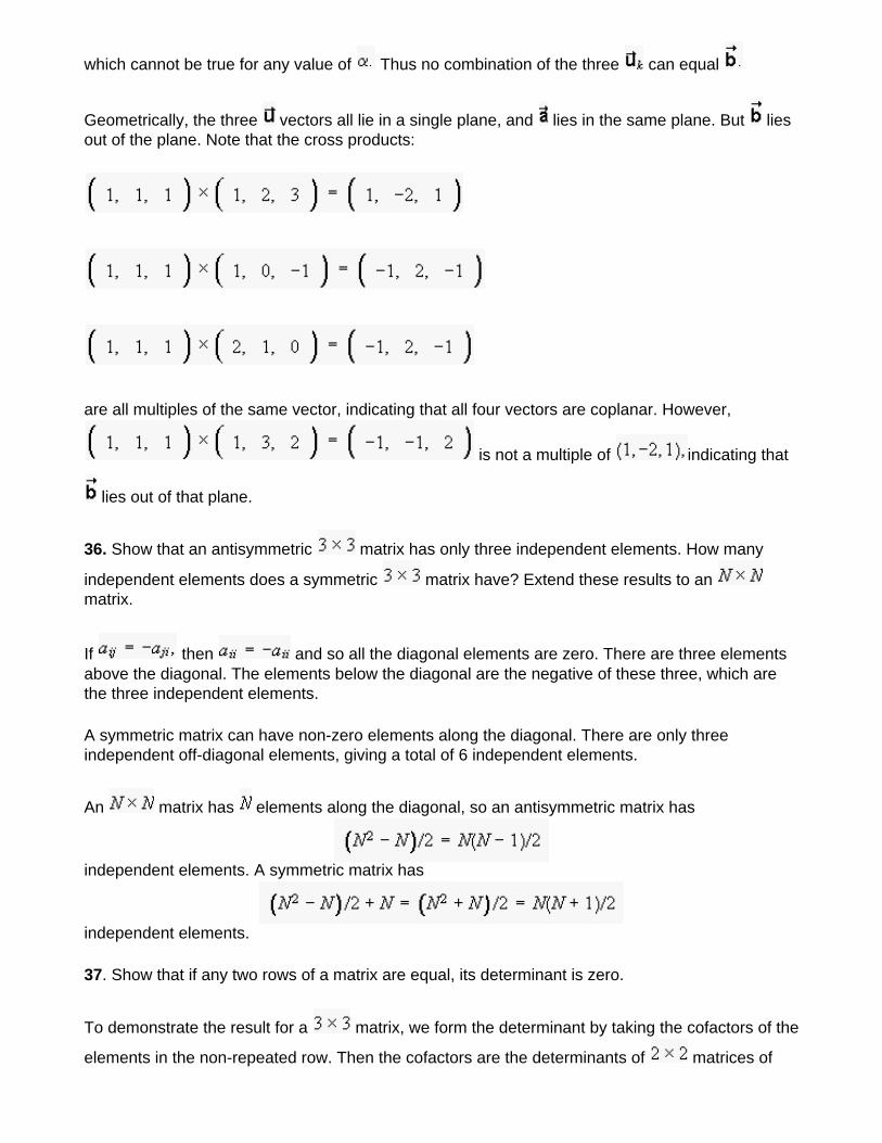
34. The vector operator appears in physics as the angular momentum operator. (Here
and is the position vector.) Prove the identity:
for an arbitrary vector
Begin with the result of problem 21:
Working on these terms one at a time:
and
Now we are left with
Now look at
The th component is
while

Substituting into our result (1.1) above:
Using equation (1.2) to evaluate we have
as required.
35. Can you express the vector as a linear combination of the vectors
and Can you express the vector as a linear
combination of the vectors and Explain your answers geometrically.
Let
Thus we have the three equations:
From the third equation
and from the second:
and so from the first:
which is true no matter what the value of Thus we can find a solution for any For example,
with
For the vector we would have:
or
which cannot be true for any value of Thus no combination of the three can equal
Geometrically, the three vectors all lie in a single plane, and lies in the same plane. But lies out of the plane. Note that the cross products:
are all multiples of the same vector, indicating that all four vectors are coplanar. However,
is not a multiple of indicating that
lies out of that plane.
36. Show that an antisymmetric matrix has only three independent elements. How many
independent elements does a symmetric matrix have? Extend these results to an matrix.
If then and so all the diagonal elements are zero. There are three elements above the diagonal. The elements below the diagonal are the negative of these three, which are the three independent elements.
A symmetric matrix can have non-zero elements along the diagonal. There are only three independent off-diagonal elements, giving a total of 6 independent elements.
An matrix has elements along the diagonal, so an antisymmetric matrix has
independent elements. A symmetric matrix has
independent elements.
37. Show that if any two rows of a matrix are equal, its determinant is zero.
To demonstrate the result for a matrix, we form the determinant by taking the cofactors of the
elements in the non-repeated row. Then the cofactors are the determinants of matrices of
the form . The determinant equals If each cofactor is zero, then the
determinant is zero. For a matrix, we can always reduce to using the Laplace development, and those determinants are zero as we have just shown.
38. Prove that a matrix with one row of zeros has a determinant equal to zero. Also show that if a
matrix is multiplied by a constant its determinant is multiplied by
Use the Laplace development, with the row of zeros as the row of chosen elements, and the result follows immediately.
Since each product in equation (1.71) in the text has three factors, the result is clearly true for a
3 3 matrix. But then, from the Laplace development, each product in a 4 determinant is one
factor times a 3 determinant, and so is times the original. Continuing in this way, we obtain the general result.
39. Prove that a matrix and its transpose have the same determinant.
Using equation 1.72 in the text (first part)
Now if is the transpose of , then
by the second part of equation 1.72.
40. Prove that the trace of a matrix is invariant under change of basis, that is,
This document created by Scientific WorkPlace 4.1.
Chapter 1: Describing the universe
41. Show that the determinant of a matrix is invariant under change of basis, i.e. det det Hence show that the determinant of a real, symmetric matrix equals the product of its eigenvalues.
For a diagonalized matrix,
QED.
42. If the product of two matrices is zero, it is not necessary that either one be zero. In particular, show that a
2 matrix whose square is zero may be written in terms of two parameters and and find the general form of the matrix.
Thus either and or If and are both zero, then and are also zero, and But if
then also Thus the matrix may be expressed in terms of the two parameters and :
43. If the product of the matrix and another non-zero matrix is zero, find the elements of
You may find it necessary to impose some conditions on matrix If so, state what they are.
We know that det so if then so Thus the product is:
Thus
which can be satisfied if in which case matrix , or In the latter case,
matrix is specified in terms of arbitrary values and as
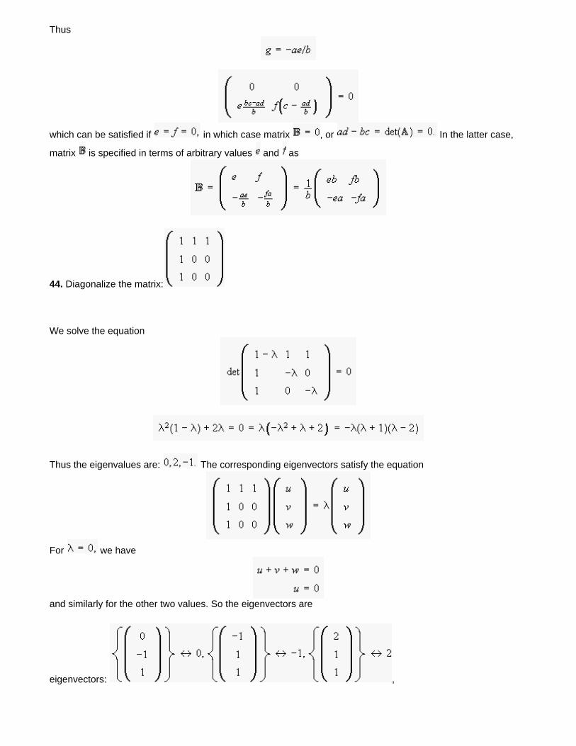
44. Diagonalize the matrix:
We solve the equation
Thus the eigenvalues are: The corresponding eigenvectors satisfy the equation
For we have
and similarly for the other two values. So the eigenvectors are
eigenvectors: ,
45. Show that a real symmetric matrix with one or more eigenvalues equal to zero has no inverse (it is singular).
Since the determinant equals the product of the eigenvalues, (Problem 41), the determinant equals zero, and thus the matrix is singular.
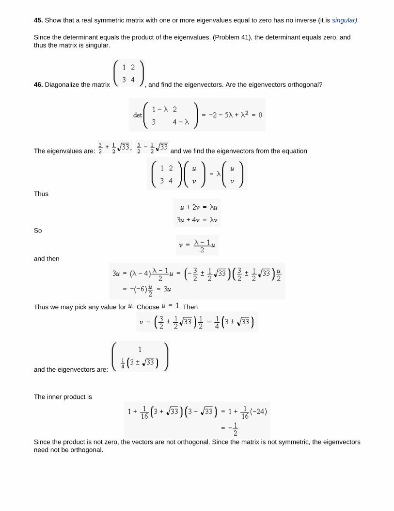
46. Diagonalize the matrix , and find the eigenvectors. Are the eigenvectors orthogonal?
The eigenvalues are: and we find the eigenvectors from the equation
Thus
So
and then
Thus we may pick any value for Choose . Then
and the eigenvectors are:
The inner product is
Since the product is not zero, the vectors are not orthogonal. Since the matrix is not symmetric, the eigenvectors need not be orthogonal.
47. What condition must be imposed on the matrix in order that with . If
and find a matrix such that .
We must have So write Then
and
We can make the two answers equal if . Then
and
48. Show that if is a real symmetric matrix and is orthogonal, then is also symmetric.
If a matrix is orthogonal, then its inverse equals its transpose, so Then:
and so is symmetric if is.
49. Show that if both and are diagonal matrices.
If and are both diagonal, then
is also diagonal. Then
and the matrices commute.
50.Let Now let similarly for and compute the product
Now if the matrix is orthogonal, then and so in this case
and the inner product is invariant.
51. A quadratic expression of the form represents a curve in the plane. (a) Write this expression in matrix form. (b) Diagonalize the matrix, and hence identify the form of the curve and find its
symmetry axes. Determine how the shape of the curve depends on the values of and Draw the curve in
the case
(a)
where the vector has components and the matrix
Check:
Now we diagonalize:
Thus the eigenvalues are:
The eigenvectors are given by:
or
The new equation is
If and are both positive, the equation is an ellipse. This happens when
But if then is negative, and the curve is an hyberbola. For the ellipse, the eigenvectors found
above give the direction of the major (minus sign in and minor axes.
For the case we have so the curve is an ellipse.
so
so
The equation of the minor axis is:
while for the major axis:
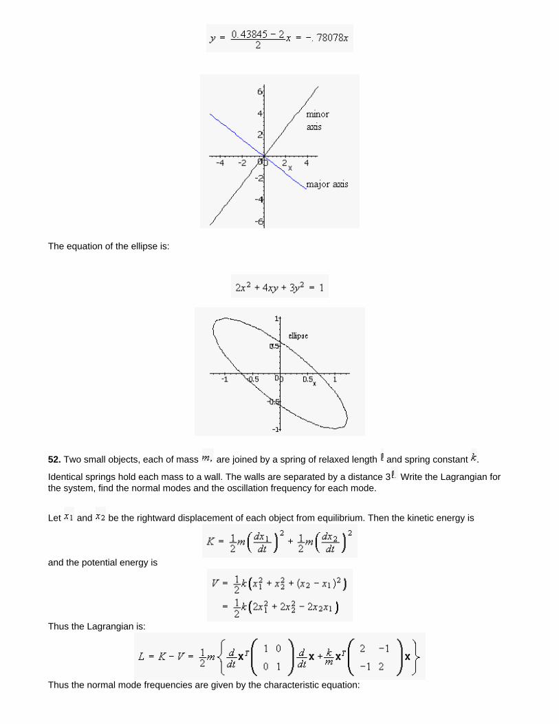
The equation of the ellipse is:
52. Two small objects, each of mass are joined by a spring of relaxed length and spring constant .
Identical springs hold each mass to a wall. The walls are separated by a distance 3 Write the Lagrangian for the system, find the normal modes and the oscillation frequency for each mode.
Let and be the rightward displacement of each object from equilibrium. Then the kinetic energy is
and the potential energy is
Thus the Lagrangian is:
Thus the normal mode frequencies are given by the characteristic equation:
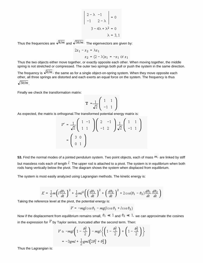
Thus the frequencies are and The eigenvectors are given by:
Thus the two objects either move together, or exactly opposite each other. When moving together, the middle spring is not stretched or compressed. The outer two springs both pull or push the system in the same direction.
The frequency is the same as for a single object-on-spring system. When they move opposite each other, all three springs are distorted and each exerts an equal force on the system. The frequency is thus
.
Finally we check the transformation matrix:
As expected, the matrix is orthogonal.The transformed potential energy matrix is:
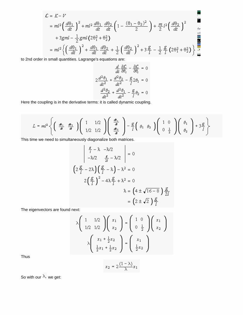
53. Find the normal modes of a jointed pendulum system. Two point objects, each of mass are linked by stiff
but massless rods each of length The upper rod is attached to a pivot. The system is in equilibrium when both rods hang vertically below the pivot. The diagram shows the system when displaced from equilibrium.
The system is most easily analyzed using Lagrangian methods. The kinetic energy is:
Taking the reference level at the pivot, the potential energy is:
Now if the displacement from equilibrium remains small, and we can approximate the cosines
in the expression for by Taylor series, truncated after the second term. Then:
Thus the Lagrangian is:
to 2nd order in small quantities. Lagrange's equations are:
Here the coupling is in the derivative terms: it is called dynamic coupling.
This time we need to simultaneously diagonalize both matrices.
The eigenvectors are found next:
Thus
So with our we get:
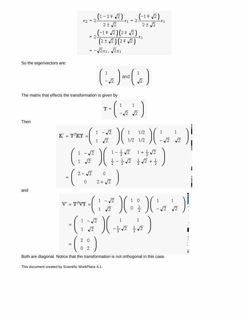
So the eigenvectors are:
The matrix that effects the transformation is given by
Then
and
Both are diagonal. Notice that the transformation is not orthogonal in this case.
This document created by Scientific WorkPlace 4.1.
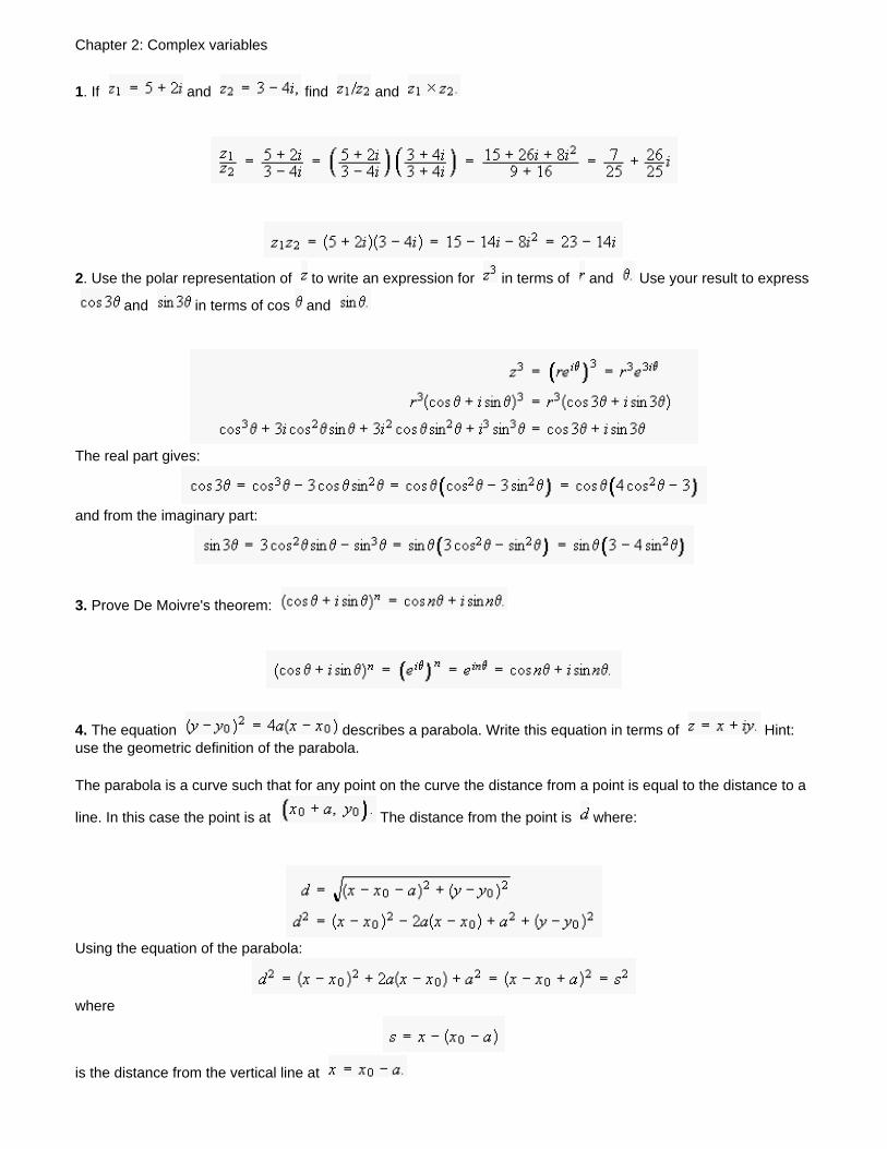
Chapter 2: Complex variables
1. If and find and
2. Use the polar representation of to write an expression for in terms of and Use your result to express
and in terms of cos and
The real part gives:
and from the imaginary part:
3. Prove De Moivre's theorem:
4. The equation describes a parabola. Write this equation in terms of Hint: use the geometric definition of the parabola.
The parabola is a curve such that for any point on the curve the distance from a point is equal to the distance to a
line. In this case the point is at The distance from the point is where:
Using the equation of the parabola:
where
is the distance from the vertical line at
Now we can express these ideas using complex numbers. The distance from the point
is and the distance from the line is Thus the equation we want is:
5. Show that the equation
represents an ellipse in the complex plane, where and are complex constants, and is a real constant. Use geometrical arguments to determine the position of the center of the ellipse and its semi-major and semi-minor axes.
The absolute value is the distance between a point in the Argand diagram described by and
the point described by the number Thus the equation describes a curve such that the sum of the distances
of from the points and is a constant ( ). This is the definition of an ellipse. The points and are
the foci of the ellipse, so its center is half way between them, at
When is at the end of the semi-major axis, then and so and the semi-major axis is
Then also
and so
6. Show that the equation
represents an ellipse in the complex plane, where and are complex constants and is a real variable. Determine the position of the center of the ellipse and its semi-major and semi-minor axes.
First recall that multiplication by corresponds to rotation counter-clockwise by an angle (Figure 2.3c) Thus
if and then is represented as follows:
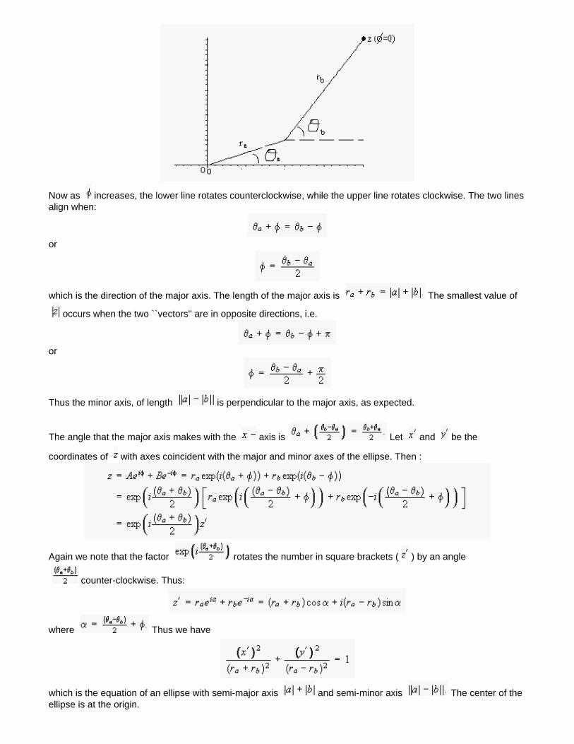
Now as increases, the lower line rotates counterclockwise, while the upper line rotates clockwise. The two lines align when:
or
which is the direction of the major axis. The length of the major axis is The smallest value of
occurs when the two ``vectors'' are in opposite directions, i.e.
or
Thus the minor axis, of length is perpendicular to the major axis, as expected.
The angle that the major axis makes with the axis is Let and be the
coordinates of with axes coincident with the major and minor axes of the ellipse. Then :
Again we note that the factor rotates the number in square brackets ( ) by an angle
counter-clockwise. Thus:
where Thus we have
which is the equation of an ellipse with semi-major axis and semi-minor axis The center of the ellipse is at the origin.
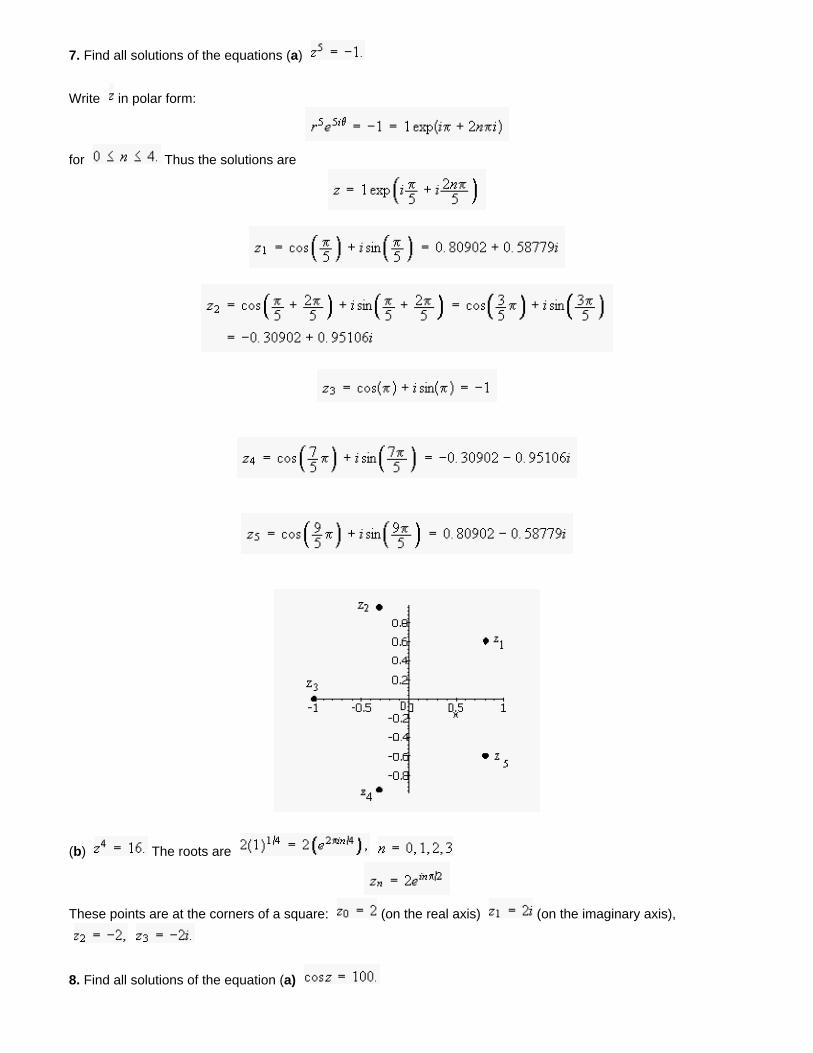
7. Find all solutions of the equations (a)
Write in polar form:
for Thus the solutions are
(b) The roots are
These points are at the corners of a square: (on the real axis) (on the imaginary axis),
8. Find all solutions of the equation (a)
Write where and are real, and expand the cosine:
Writing the real and imaginary parts separately, we have:
We can solve the second equation with either or But with the first equation becomes
, which has no solutions. (Remember that is real.) So we must choose where is any positive or negative integer, or zero. Then:
Now the hyperbolic cosine is always positive if is real, so we must choose to be even, or zero. Then
and:
and thus
or
Both values give the same value for the cosh. Then
(b)
Equating real and imaginary parts:
Clearly is not a viable solution, so we need
Then
Since cosh is always positive ( is real) then must be even, and
Thus
Thus
9. Find all solutions of the equation
The imaginary part must
be zero, so we must have or The real part would be or in the two cases.
Since can never equal we must choose with odd, and then setting the real part equal to
we need
and the solution is : Thus where is any positive or negative integer.
10. Find all numbers such that
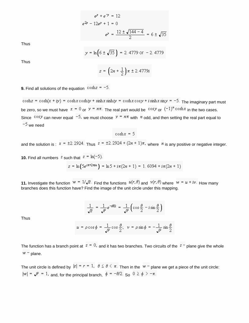
11. Investigate the function Find the functions and where How many branches does this function have? Find the image of the unit circle under this mapping.
Thus
The function has a branch point at and it has two branches. Two circuits of the plane give the whole
plane.
The unit circle is defined by Then in the plane we get a piece of the unit circle:
and, for the principal branch, So
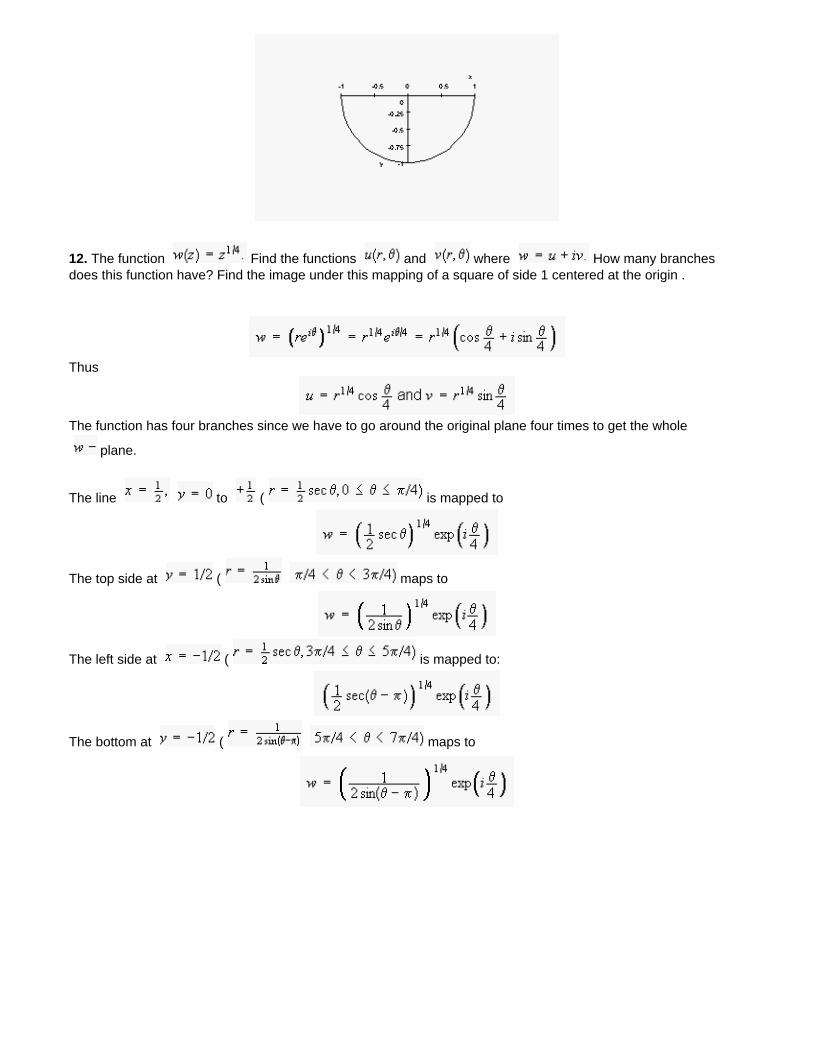
12. The function Find the functions and where How many branches does this function have? Find the image under this mapping of a square of side 1 centered at the origin .
Thus
The function has four branches since we have to go around the original plane four times to get the whole
plane.
The line to ( is mapped to
The top side at ( maps to
The left side at ( is mapped to:
The bottom at ( maps to
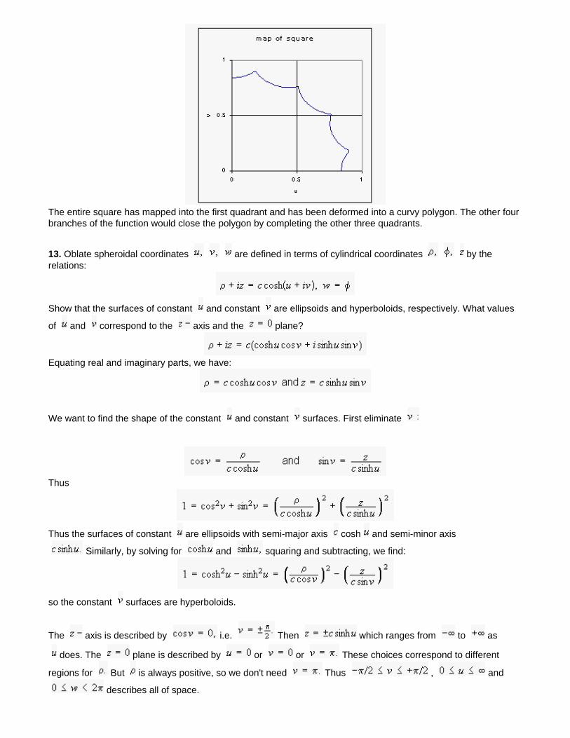
The entire square has mapped into the first quadrant and has been deformed into a curvy polygon. The other four branches of the function would close the polygon by completing the other three quadrants.
13. Oblate spheroidal coordinates are defined in terms of cylindrical coordinates by the relations:
Show that the surfaces of constant and constant are ellipsoids and hyperboloids, respectively. What values
of and correspond to the axis and the plane?
Equating real and imaginary parts, we have:
We want to find the shape of the constant and constant surfaces. First eliminate
Thus
Thus the surfaces of constant are ellipsoids with semi-major axis cosh and semi-minor axis
Similarly, by solving for and squaring and subtracting, we find:
so the constant surfaces are hyperboloids.
The axis is described by i.e. Then which ranges from to as
does. The plane is described by or or These choices correspond to different
regions for But is always positive, so we don't need Thus , and
describes all of space.
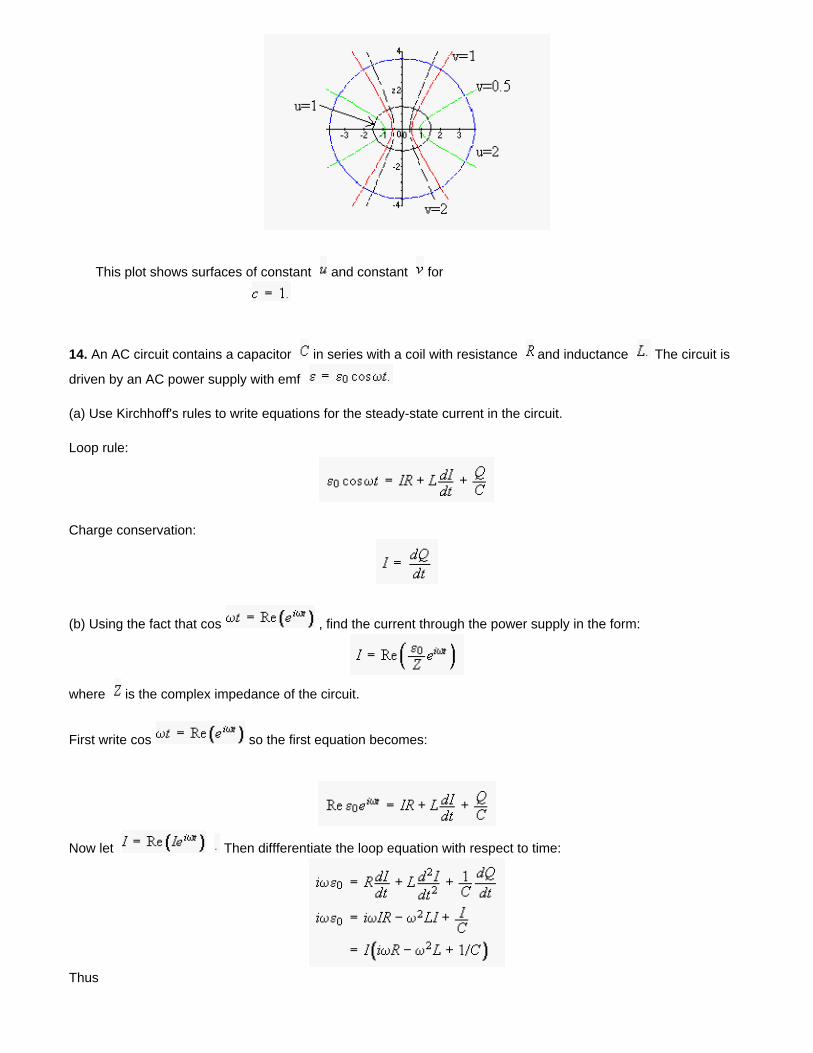
This plot shows surfaces of constant and constant for
14. An AC circuit contains a capacitor in series with a coil with resistance and inductance The circuit is
driven by an AC power supply with emf
(a) Use Kirchhoff's rules to write equations for the steady-state current in the circuit.
Loop rule:
Charge conservation:
(b) Using the fact that cos , find the current through the power supply in the form:
where is the complex impedance of the circuit.
First write cos so the first equation becomes:
Now let Then diffferentiate the loop equation with respect to time:
Thus
The complex impedance is:
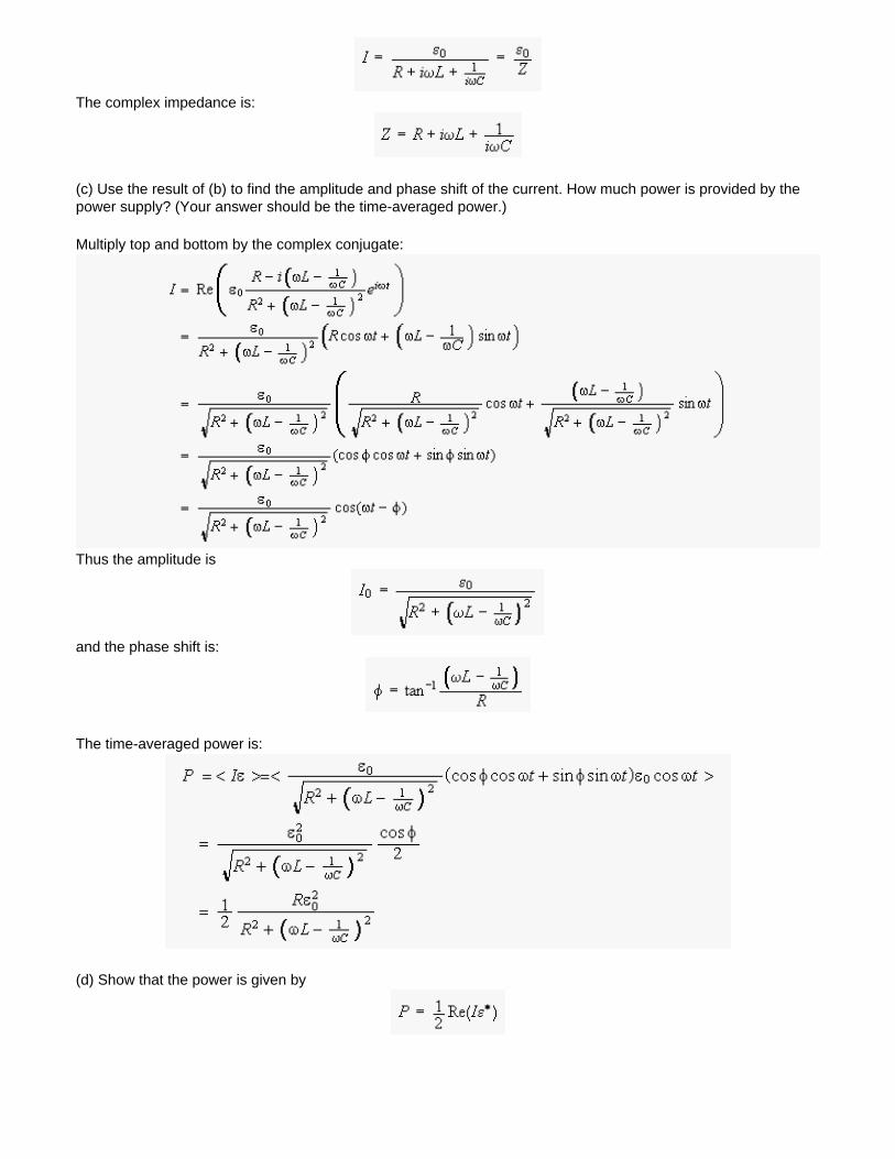
(c) Use the result of (b) to find the amplitude and phase shift of the current. How much power is provided by the power supply? (Your answer should be the time-averaged power.)
Multiply top and bottom by the complex conjugate:
Thus the amplitude is
and the phase shift is:
The time-averaged power is:
(d) Show that the power is given by
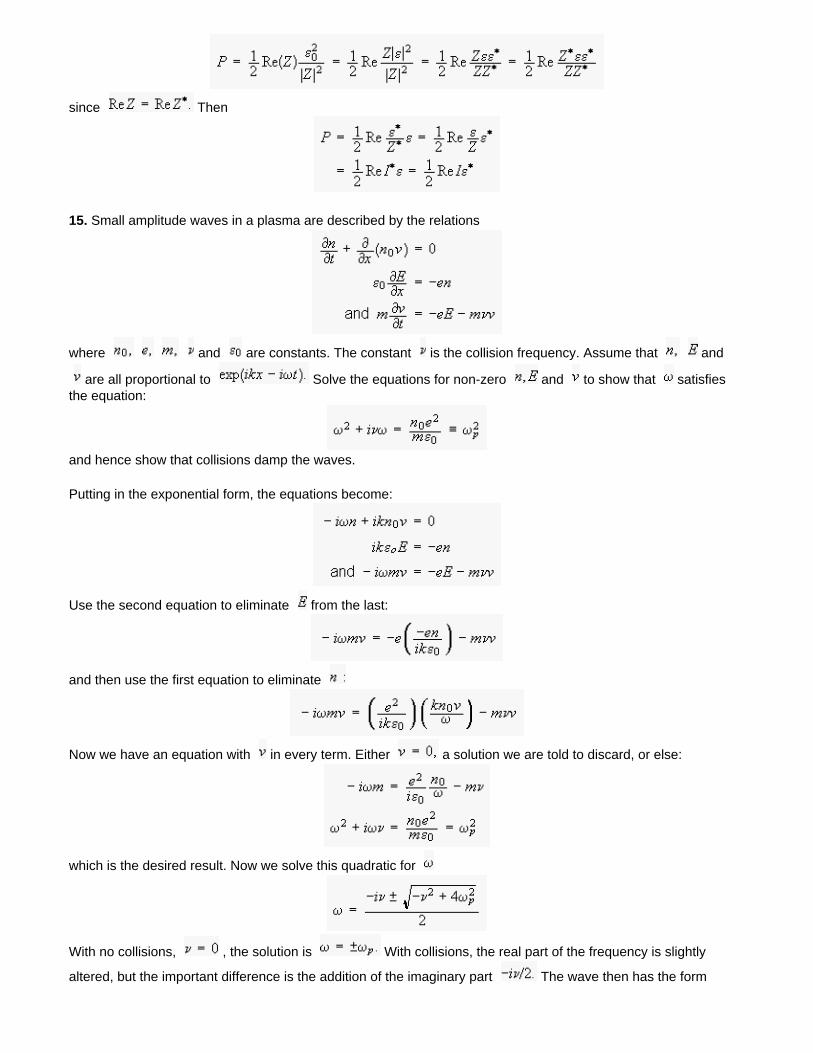
since Then
15. Small amplitude waves in a plasma are described by the relations
where and are constants. The constant is the collision frequency. Assume that and
are all proportional to Solve the equations for non-zero and to show that satisfies the equation:
and hence show that collisions damp the waves.
Putting in the exponential form, the equations become:
Use the second equation to eliminate from the last:
and then use the first equation to eliminate
Now we have an equation with in every term. Either a solution we are told to discard, or else:
which is the desired result. Now we solve this quadratic for
With no collisions, , the solution is With collisions, the real part of the frequency is slightly
altered, but the important difference is the addition of the imaginary part The wave then has the form
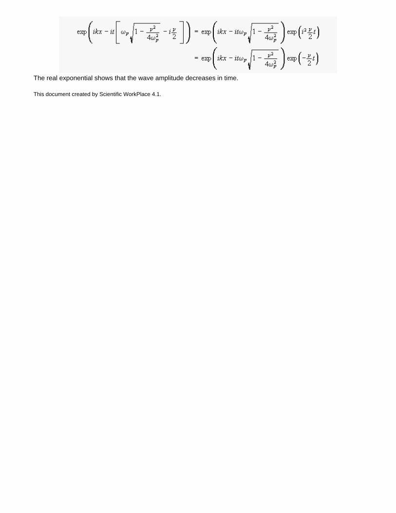
The real exponential shows that the wave amplitude decreases in time.
This document created by Scientific WorkPlace 4.1.
Chapter 2: Complex variables
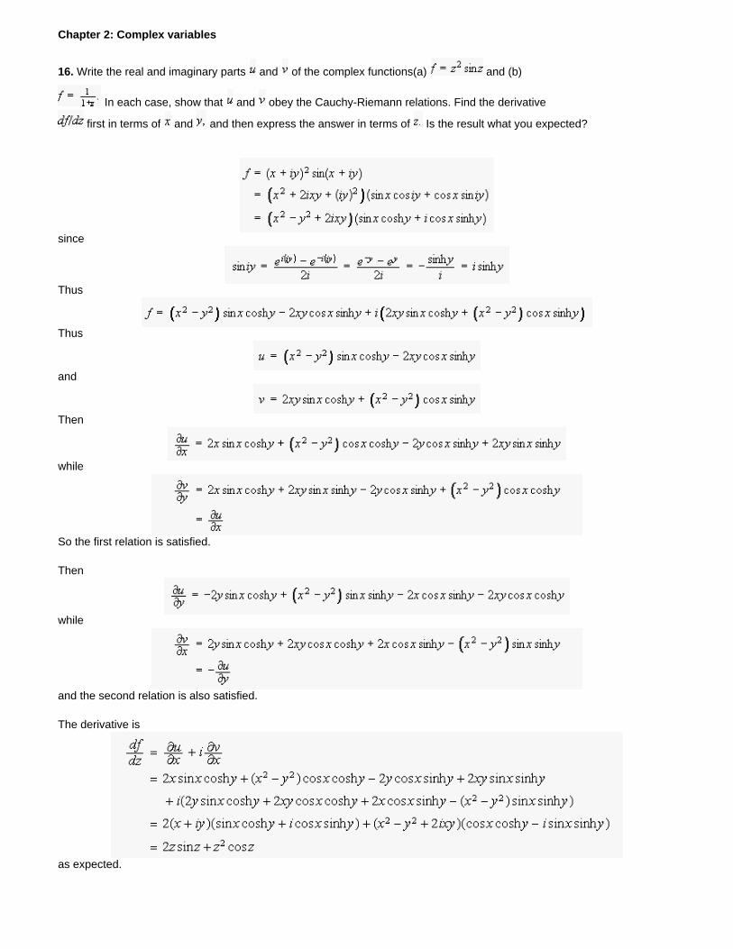
16. Write the real and imaginary parts and of the complex functions(a) and (b)
In each case, show that and obey the Cauchy-Riemann relations. Find the derivative
first in terms of and and then express the answer in terms of Is the result what you expected?
since
Thus
Thus
and
Then
while
So the first relation is satisfied.
Then
while
and the second relation is also satisfied.
The derivative is
as expected.
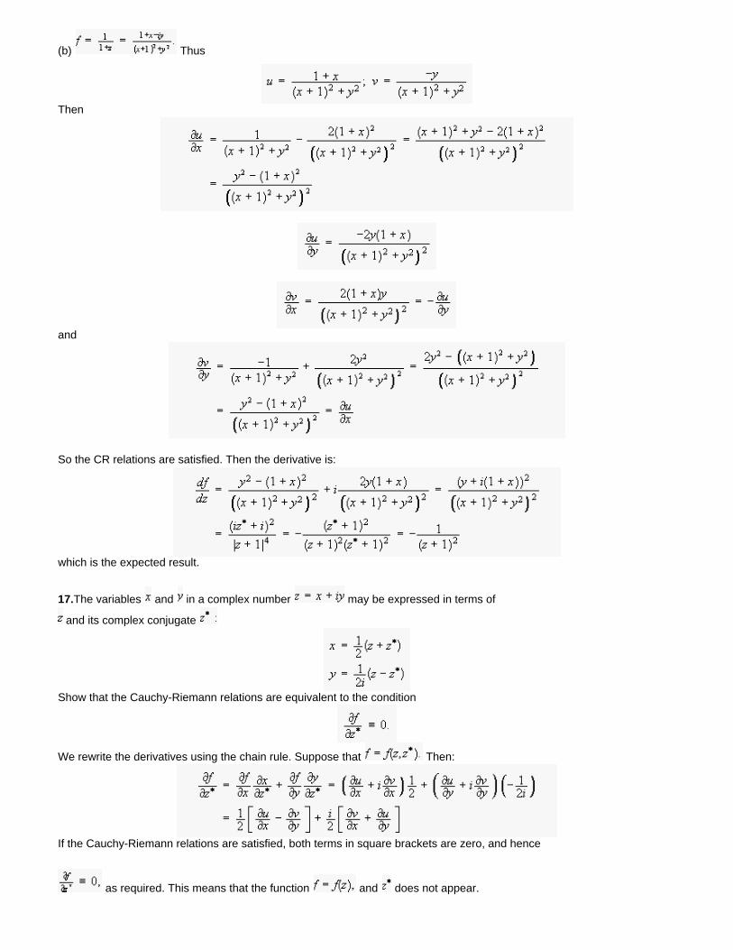
(b) Thus
Then
and
So the CR relations are satisfied. Then the derivative is:
which is the expected result.
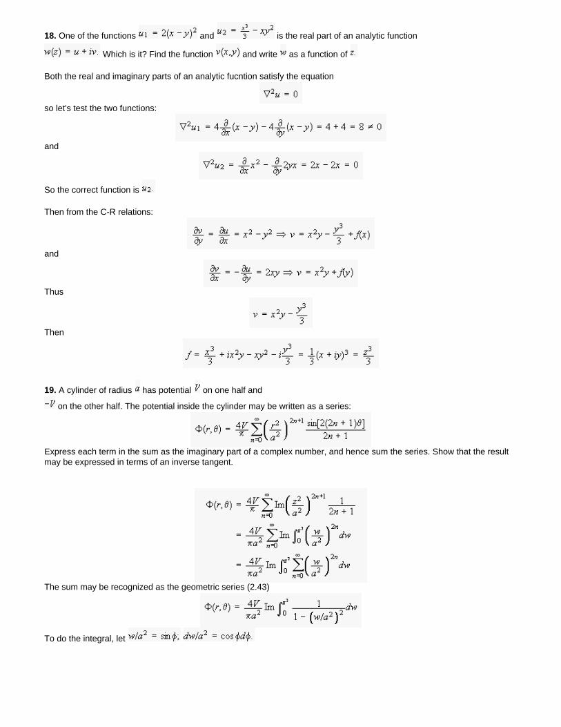
17.The variables and in a complex number may be expressed in terms of
and its complex conjugate
Show that the Cauchy-Riemann relations are equivalent to the condition
We rewrite the derivatives using the chain rule. Suppose that Then:
If the Cauchy-Riemann relations are satisfied, both terms in square brackets are zero, and hence
as required. This means that the function and does not appear.
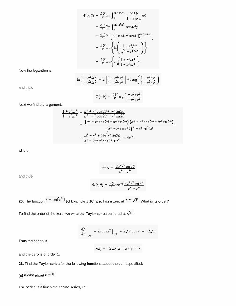
18. One of the functions and is the real part of an analytic function
Which is it? Find the function and write as a function of
Both the real and imaginary parts of an analytic fucntion satisfy the equation
so let's test the two functions:
and
So the correct function is
Then from the C-R relations:
and
Thus
Then
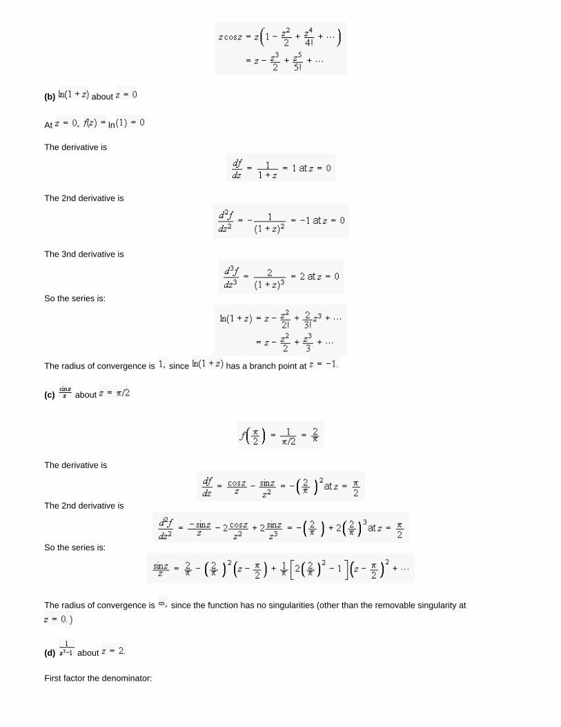
19. A cylinder of radius has potential on one half and
on the other half. The potential inside the cylinder may be written as a series:
Express each term in the sum as the imaginary part of a complex number, and hence sum the series. Show that the result may be expressed in terms of an inverse tangent.
The sum may be recognized as the geometric series (2.43)
To do the integral, let
Now the logarithm is
and thus
Next we find the argument:
where
and thus
20. The function (cf Example 2.10) also has a zero at What is its order?
To find the order of the zero, we write the Taylor series centered at
Thus the series is
and the zero is of order 1.
21. Find the Taylor series for the following functions about the point specified:
(a) about
The series is times the cosine series, i.e.
(b) about
At ln
The derivative is
The 2nd derivative is
The 3nd derivative is
So the series is:
The radius of convergence is since has a branch point at
(c) about
The derivative is
The 2nd derivative is
So the series is:
The radius of convergence is since the function has no singularities (other than the removable singularity at
(d) about
First factor the denominator:
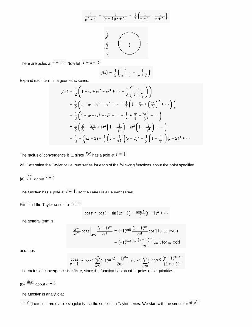
There are poles at Now let
Expand each term in a geometric series:
The radius of convergence is 1, since has a pole at
22. Determine the Taylor or Laurent series for each of the following functions about the point specified:
(a) about
The function has a pole at so the series is a Laurent series.
First find the Taylor series for
The general term is
and thus
The radius of convergence is infinite, since the function has no other poles or singularities.
(b) about
The function is analytic at
(there is a removable singularity) so the series is a Taylor series. We start with the series for
The radius of convergence is infinite, since the function has no poles or other singularities
(c) about
There is a simple pole at the series is a Laurent series:
The radius of convergence is infinite, since the function has no other poles or singularities.
(d) about
Th function has a branch point at . The singularity at is removable, since has a zero at
We should be able to find a Taylor series valid for
First find the Taylor series for Let
So
(e) tan
So
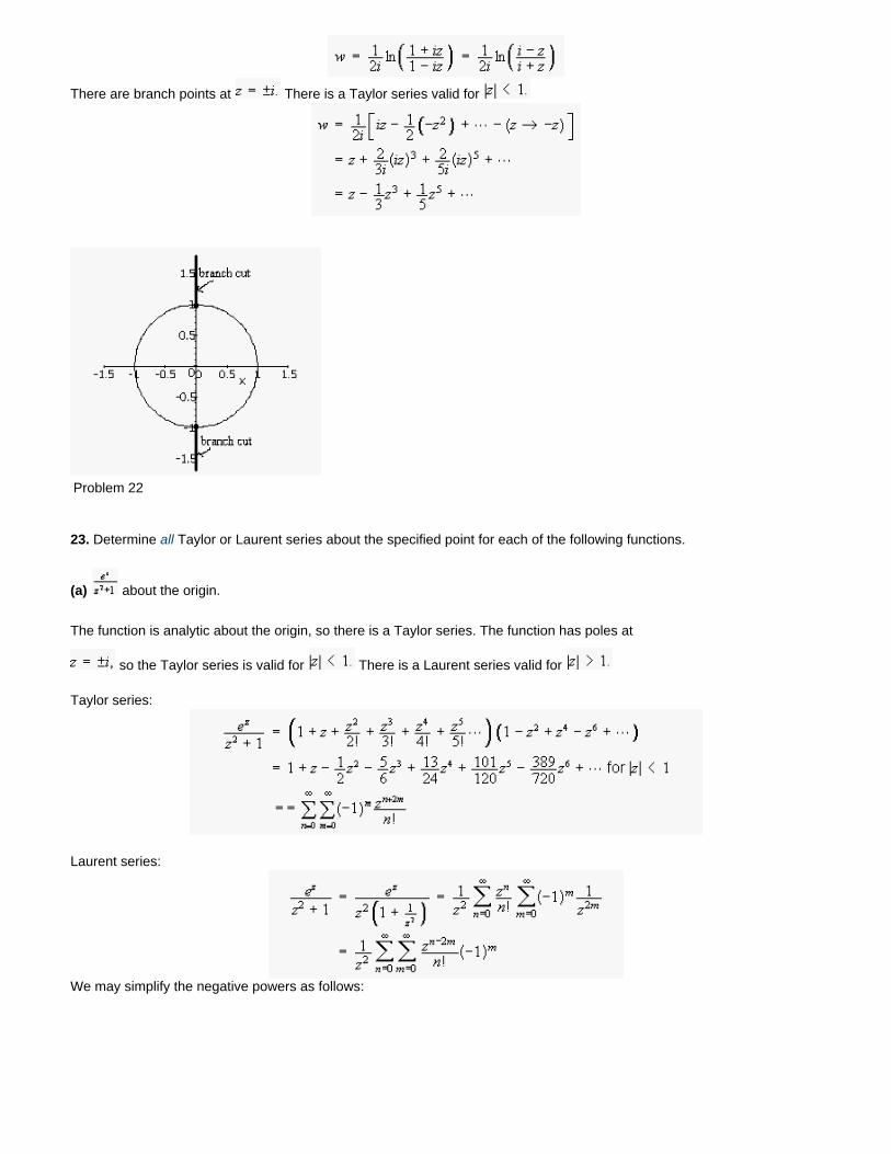
There are branch points at There is a Taylor series valid for
Problem 22
23. Determine all Taylor or Laurent series about the specified point for each of the following functions.
(a) about the origin.
The function is analytic about the origin, so there is a Taylor series. The function has poles at
so the Taylor series is valid for There is a Laurent series valid for
Taylor series:
Laurent series:
We may simplify the negative powers as follows:
valid for
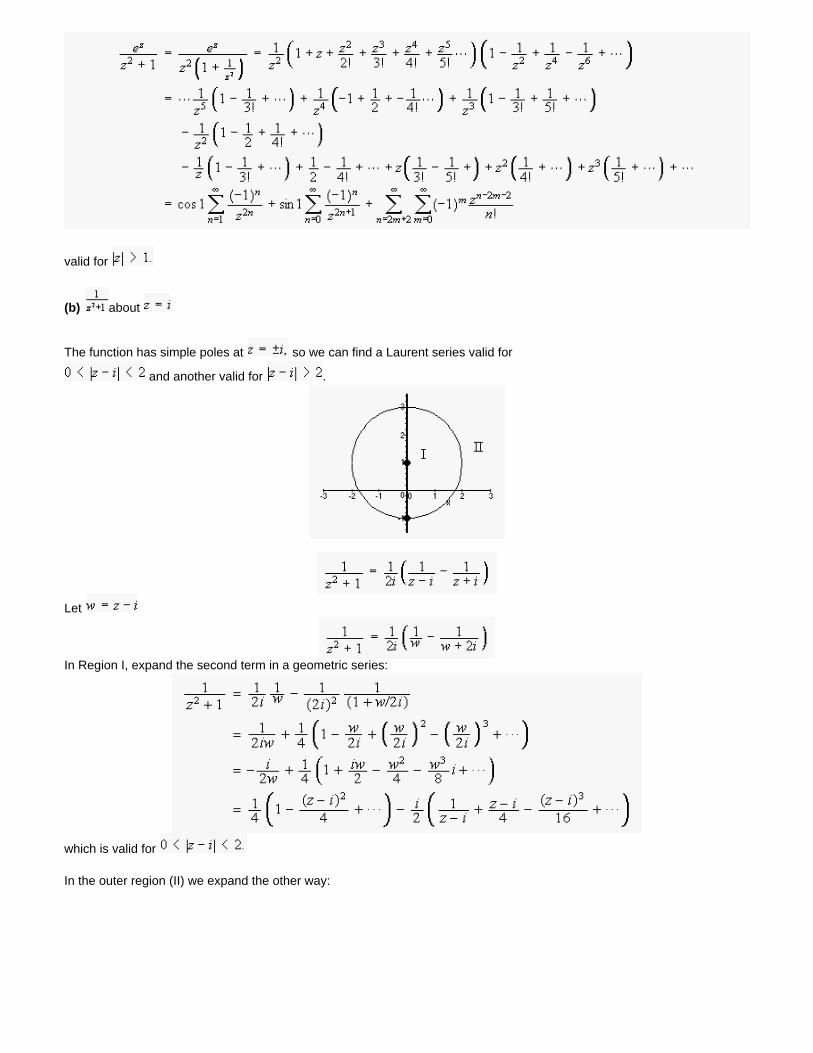
(b) about
The function has simple poles at so we can find a Laurent series valid for
and another valid for .
Let
In Region I, expand the second term in a geometric series:
which is valid for
In the outer region (II) we expand the other way:
which is valid for
(c) about
The function has poles at We should be able to find a Laurent series valid for
and another for
where Then for we have:
while for
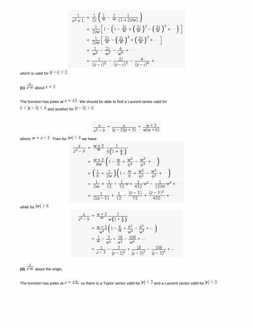
(d) about the origin.
The function has poles at so there is a Taylor series valid for and a Laurent series valid for
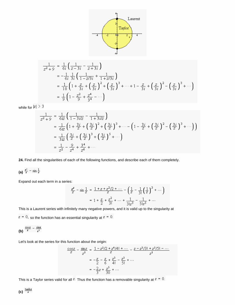
while for
24. Find all the singularities of each of the following functions, and describe each of them completely.
(a)
Expand out each term in a series:
This is a Laurent series with infinitely many negative powers, and it is valid up to the singularity at
so the function has an essential singularity at
(b)
Let's look at the series for this function about the origin:
This is a Taylor series valid for all Thus the function has a removable singularity at
(c)
The function has a removable singularity at
But the tanh function also has singularities regularly spaced along the imaginary axis.
and has singularities at The singularities are all simple poles. For example
Since the limit exists, the pole is simple.
(d)
The function has a branch point where or
25. Incompressible fluid flows over a thin sheet from a distance
into a corner as shown in the diagram. The angle between the barriers is and at
Assuming that the flow is as simple as possible, determine the streamlines of the flow. What is the velocity at
The velocity potential satsifies
and thus we may look for a complex potential . must be an analytic function in the region
, and at we need
The streamline function must be a constant on the surfaces and

We may take this constant to be zero, and then the function does the job. (The function
would also work, but would lead to more complicated flow.) This suggests that we look at the analytic function
The imaginary part of this function satisfies the boundary conditions at the two surfaces. Thus the streamlines are given by
and the velocity is given by
Thus at we have
and so
Thus the streamlines are given by
See Figure. (solid line), 5 (dashes), and 1/5 (dots).
The velocity is
and so at we have
This document created by Scientific WorkPlace 4.1.
Chapter 2: Complex variables
26. Prove the Schwarz reflection principle: If a function is analytic in a region including the real axis, and
is real when is real,
Show that the result may be extended to functions that posess a Laurent series about the origin with real coefficients.
Verify the result for the functions (a) and (b)
(c) Show that the result does not hold for all if (the principal branch is assumed).
If the function is analytic, it may be expanded in a Taylor series about a point on the real axis:
and since
is real, then each of the must be real. Then
The proof extends trivially to the case where the series is a Laurent series with real coefficients.
So
The function is trickier.
Thus
and, choosing the principal branch of the logarithm,
Then
and
and the two expressions are the same.
Note that this function has branch points at but it is analytic on the real axis.
(c)
We proceed by showing that the relation fails at one point, At on the real axis,
Then
but
27. Find the residues of each of the following functions at the point specified.
(a) at
First factor the function:
The function has a simple pole at and the residue is:
(b) at
First rewrite the function:
and then expand in a Laurent series:
Now we can pick out the residue: it is the coefficient of The residue is
(c) at the origin
The easiest method here is to find the Laurent series:
and thus the residue is
1.
(d) at
Since the denominator is a function that has a simple zero at we can use method 4. The derivative is
and so
28. Evaluate the following integrals:
(a) where is a circle of radius centered at the origin.
The integrand has a simple pole at which is inside the circle. The residue there is:
and thus
(b) where is a square of side 4 centered at the origin.
The integrand has a simple pole at which is inside the square. The residue there is:
and thus

(c) where is a circle of radius centered at the origin.
The integrand has a pole at which is outside the circle. Thus:
(d) where is a square of side 1 centered at the point
The integrand has two simple poles, at Only one, at is inside the square. The residue at
is
and so
29. Evaluate the following integrals:
(a)
We evaluate as an ingtegral around the unit circle. Let Then
and
and
Then
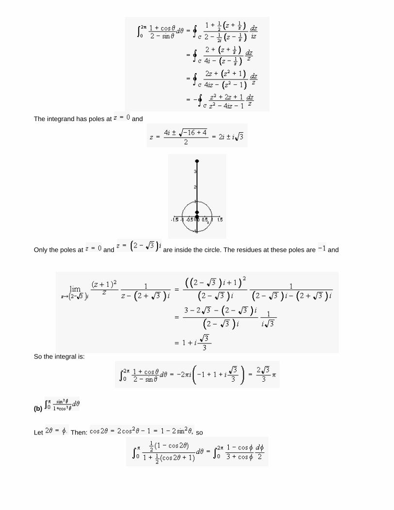
The integrand has poles at and
Only the poles at and are inside the circle. The residues at these poles are and
So the integral is:
(b)
Let Then: so
The integrand has poles where
Only one of these poles is inside the unit circle. There is an additional pole at The residues are and:
Thus the integral is:
(c)
The integrand has poles where
Of these 4 poles only 2 are inside the circle, at and The residues are:
and
Thus the integral is:
(d)
Since sin we may rewrite the integral:
The integrand has a pole of order at The residue is:
All the terms in powers are zero in the limit, and all the terms in powers differentiate away. Thus
Thus the integral is:
30. Evaluate each of the following integrals:
(a)
We close the contour with a big semicircle at infinity. The integral over the semicircle is:
The poles of the integrand are at Only the pole at is inside the contour. the residue is:
and the integral is:
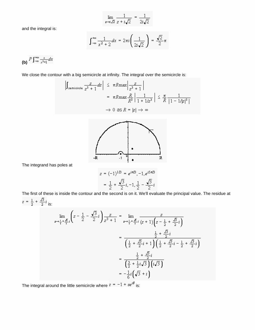
(b)
We close the contour with a big semicircle at infinity. The integral over the semicircle is:
The integrand has poles at
The first of these is inside the contour and the second is on it. We'll evaluate the principal value. The residue at
is:
The integral around the little semicircle where is:
Thus
and so
(c)
There are no poles on the real axis, so we may assume that the integral is real. Then we may evaluate:
Close the contour with a big semicircle in the upper half plane. The integral along the semicircle is zero by
Jordan's lemma. The poles are at but only the pole at is inside the contour. The residue is:
Then:
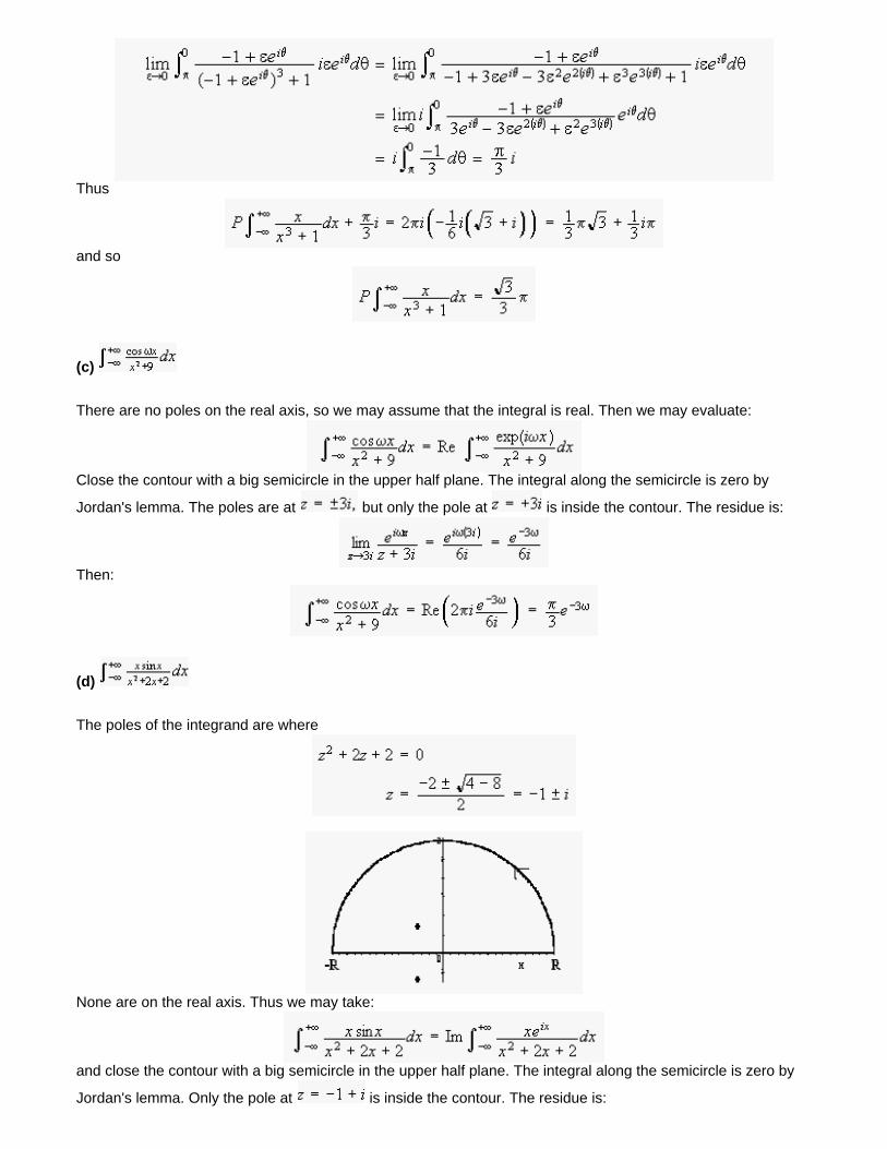
(d)
The poles of the integrand are where
None are on the real axis. Thus we may take:
and close the contour with a big semicircle in the upper half plane. The integral along the semicircle is zero by
Jordan's lemma. Only the pole at is inside the contour. The residue is:
Thus the integral is:
This document created by Scientific WorkPlace 4.1.
Chapter 2: Complex variables
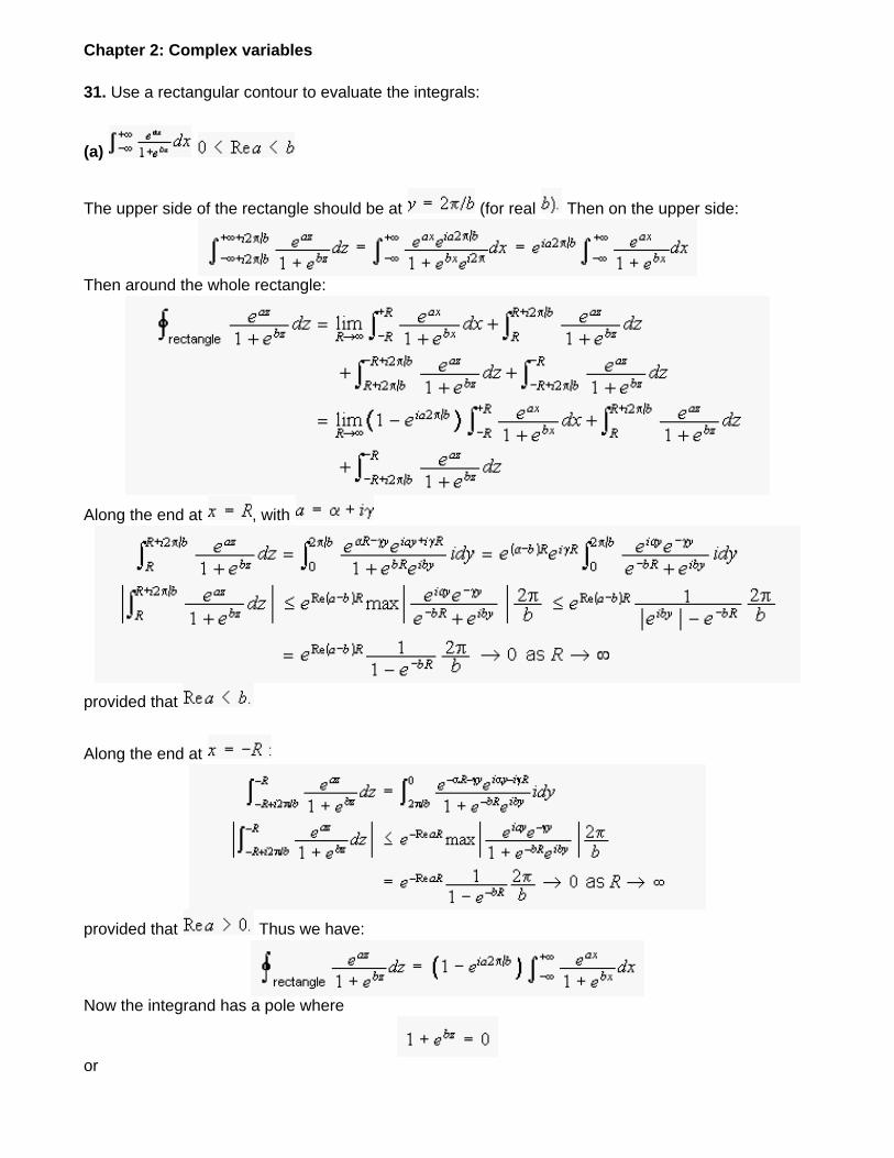
31. Use a rectangular contour to evaluate the integrals:
(a)
The upper side of the rectangle should be at (for real Then on the upper side:
Then around the whole rectangle:
Along the end at , with
provided that
Along the end at
provided that Thus we have:
Now the integrand has a pole where
or
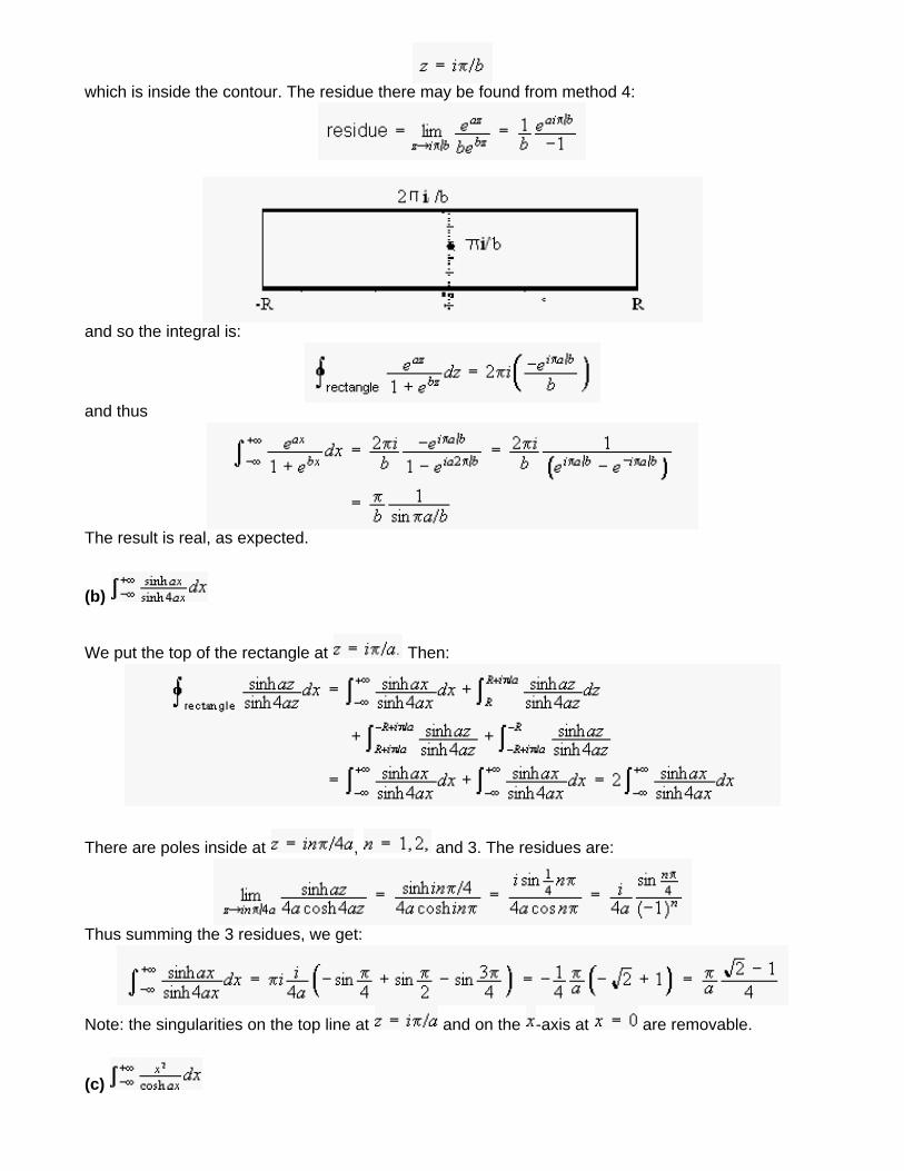
which is inside the contour. The residue there may be found from method 4:
and so the integral is:
and thus
The result is real, as expected.
(b)
We put the top of the rectangle at Then:
There are poles inside at , and 3. The residues are:
Thus summing the 3 residues, we get:
Note: the singularities on the top line at and on the -axis at are removable.
(c)
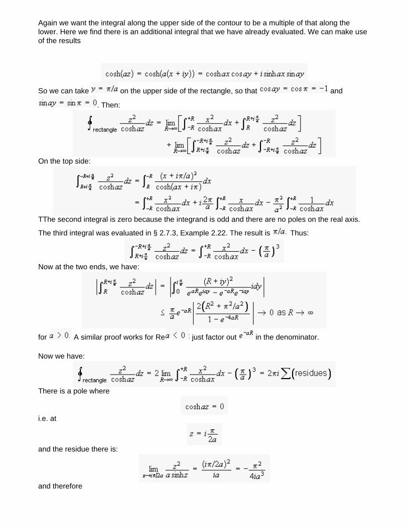
Again we want the integral along the upper side of the contour to be a multiple of that along the lower. Here we find there is an additional integral that we have already evaluated. We can make use of the results
So we can take on the upper side of the rectangle, so that and
. Then:
On the top side:
TThe second integral is zero because the integrand is odd and there are no poles on the real axis.
The third integral was evaluated in § 2.7.3, Example 2.22. The result is Thus:
Now at the two ends, we have:
for A similar proof works for Re just factor out in the denominator.
Now we have:
There is a pole where
i.e. at
and the residue there is:
and therefore
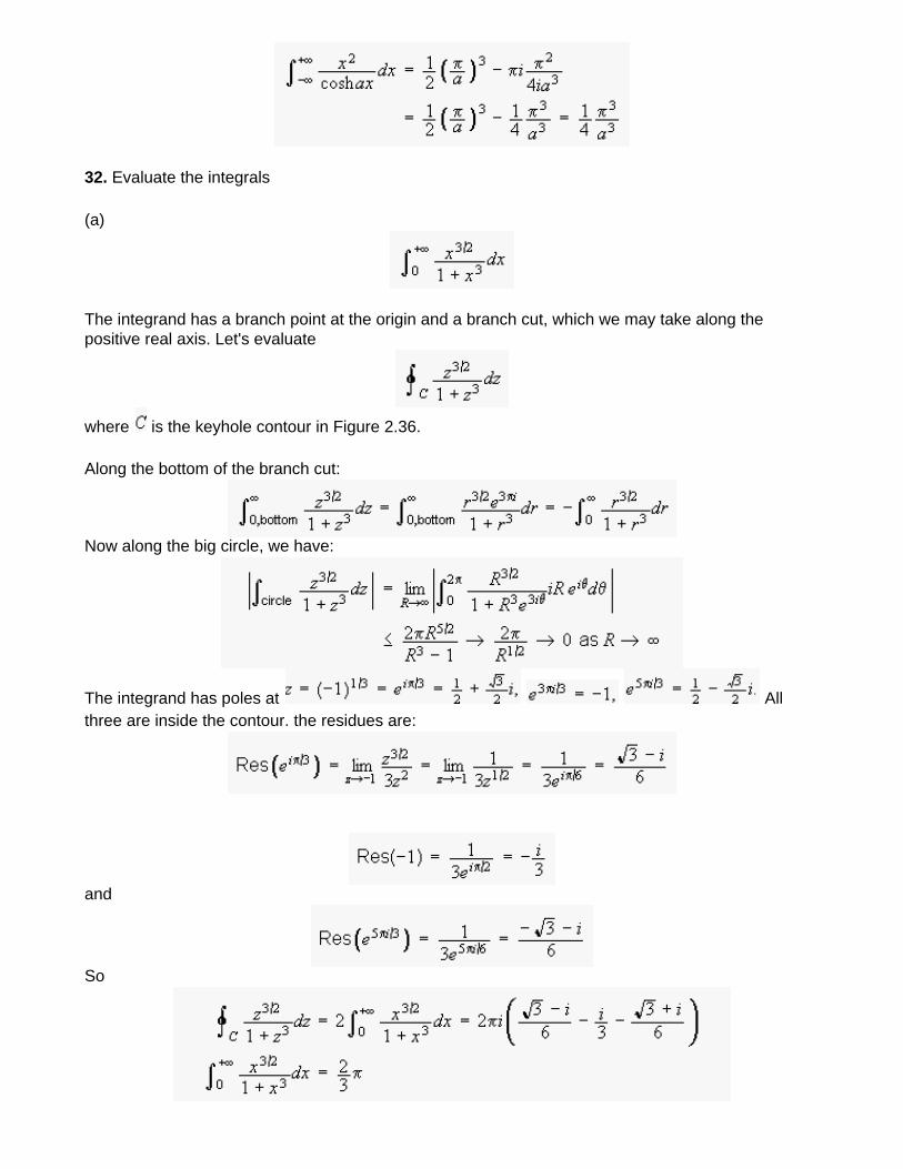
32. Evaluate the integrals
(a)
The integrand has a branch point at the origin and a branch cut, which we may take along the positive real axis. Let's evaluate
where is the keyhole contour in Figure 2.36.
Along the bottom of the branch cut:
Now along the big circle, we have:
The integrand has poles at All three are inside the contour. the residues are:
and
So
(b)
Use the keyhole contour. There are two poles inside, at that is, and
Check that the integral around the small circle goes to zero:
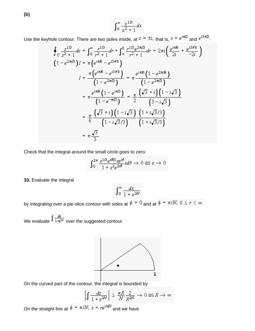
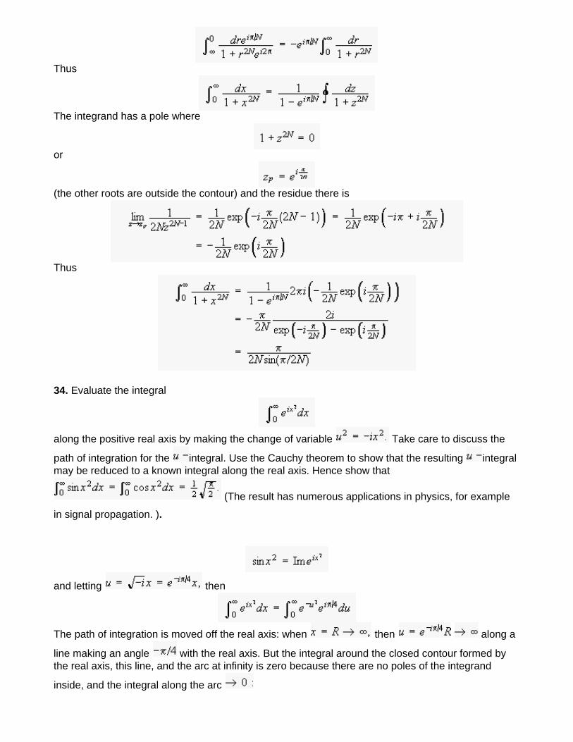
33. Evaluate the integral
by integrating over a pie-slice contour with sides at and at
We evaluate over the suggested contour.
On the curved part of the contour, the integral is bounded by
On the straight line at and we have
Thus
The integrand has a pole where
or
(the other roots are outside the contour) and the residue there is
Thus
34. Evaluate the integral
along the positive real axis by making the change of variable Take care to discuss the
path of integration for the integral. Use the Cauchy theorem to show that the resulting integral may be reduced to a known integral along the real axis. Hence show that
(The result has numerous applications in physics, for example
in signal propagation. ).
and letting then
The path of integration is moved off the real axis: when then along a
line making an angle with the real axis. But the integral around the closed contour formed by the real axis, this line, and the arc at infinity is zero because there are no poles of the integrand
inside, and the integral along the arc
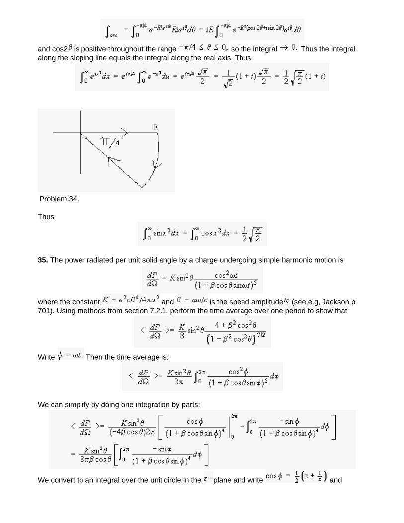
and cos2 is positive throughout the range so the integral Thus the integral along the sloping line equals the integral along the real axis. Thus
Problem 34.
Thus
35. The power radiated per unit solid angle by a charge undergoing simple harmonic motion is
where the constant and is the speed amplitude (see.e.g, Jackson p 701). Using methods from section 7.2.1, perform the time average over one period to show that
Write Then the time average is:
We can simplify by doing one integration by parts:
We convert to an integral over the unit circle in the plane and write and
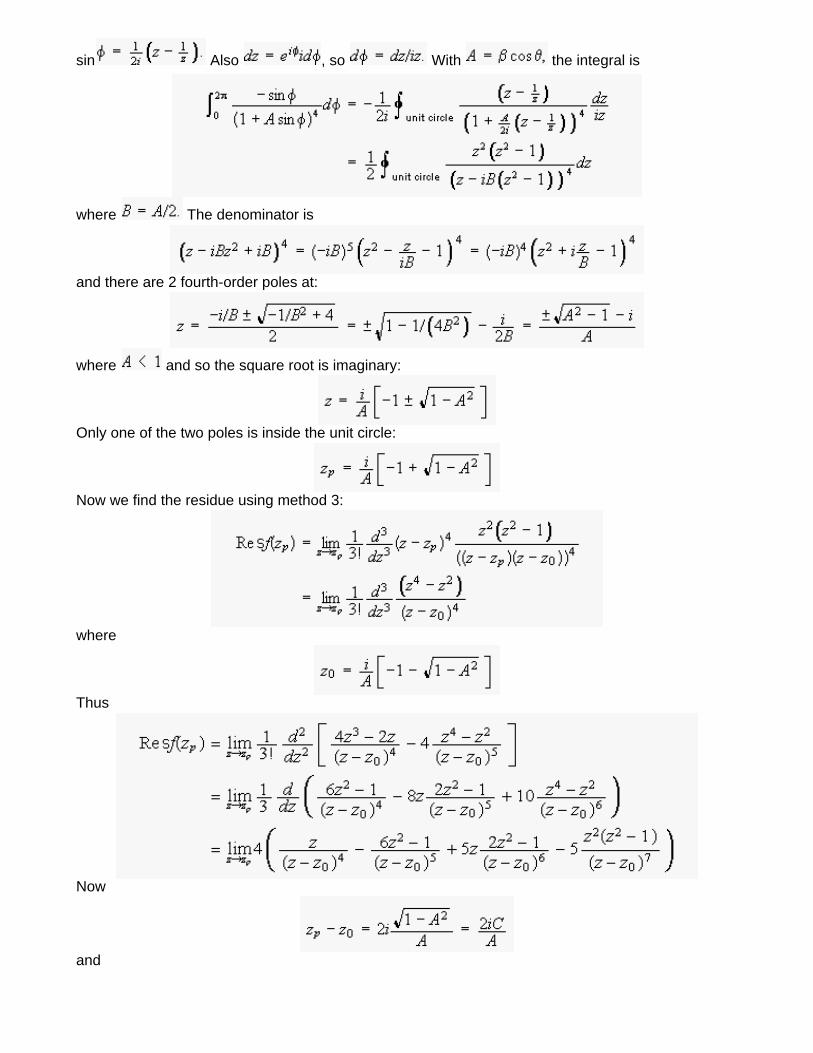
sin Also , so With the integral is
where The denominator is
and there are 2 fourth-order poles at:
where and so the square root is imaginary:
Only one of the two poles is inside the unit circle:
Now we find the residue using method 3:
where
Thus
Now
and
So
Thus
and thus the integral is:
and finally
as required.
This document created by Scientific WorkPlace 4.1.
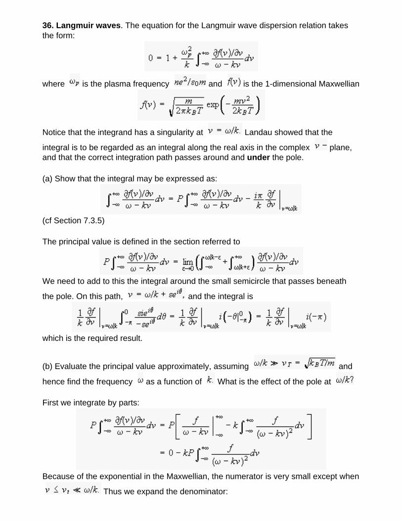
36. Langmuir waves. The equation for the Langmuir wave dispersion relation takes the form:
where is the plasma frequency and is the 1-dimensional Maxwellian
Notice that the integrand has a singularity at Landau showed that the
integral is to be regarded as an integral along the real axis in the complex plane, and that the correct integration path passes around and under the pole.
(a) Show that the integral may be expressed as:
(cf Section 7.3.5)
The principal value is defined in the section referred to
We need to add to this the integral around the small semicircle that passes beneath
the pole. On this path, and the integral is
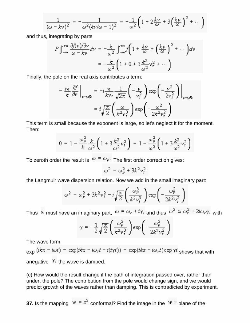
which is the required result.
(b) Evaluate the principal value approximately, assuming and
hence find the frequency as a function of What is the effect of the pole at
First we integrate by parts:
Because of the exponential in the Maxwellian, the numerator is very small except when
Thus we expand the denominator:
and thus, integrating by parts
Finally, the pole on the real axis contributes a term:
This term is small because the exponent is large, so let's neglect it for the moment. Then:
To zeroth order the result is The first order correction gives:
the Langmuir wave dispersion relation. Now we add in the small imaginary part:
Thus must have an imaginary part, and thus with
The wave form
exp shows that with
anegative the wave is damped.
(c) How would the result change if the path of integration passed over, rather than under, the pole? The contribution from the pole would change sign, and we would predict growth of the waves rather than damping. This is contradicted by experiment.
37. Is the mapping conformal? Find the image in the plane of the
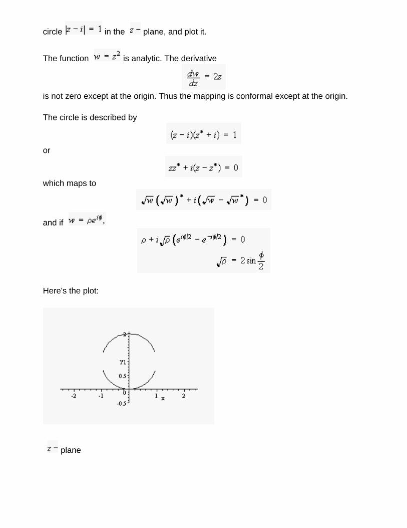
circle in the plane, and plot it.
The function is analytic. The derivative
is not zero except at the origin. Thus the mapping is conformal except at the origin.
The circle is described by
or
which maps to
and if
Here's the plot:
plane
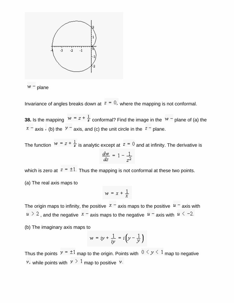
plane
Invariance of angles breaks down at where the mapping is not conformal.
38. Is the mapping conformal? Find the image in the plane of (a) the
axis (b) the axis, and (c) the unit circle in the plane.
The function is analytic except at and at infinity. The derivative is
which is zero at Thus the mapping is not conformal at these two points.
(a) The real axis maps to
The origin maps to infinity, the positive axis maps to the positive axis with
, and the negative axis maps to the negative axis with
(b) The imaginary axis maps to
Thus the points map to the origin. Points with map to negative
while points with map to positive
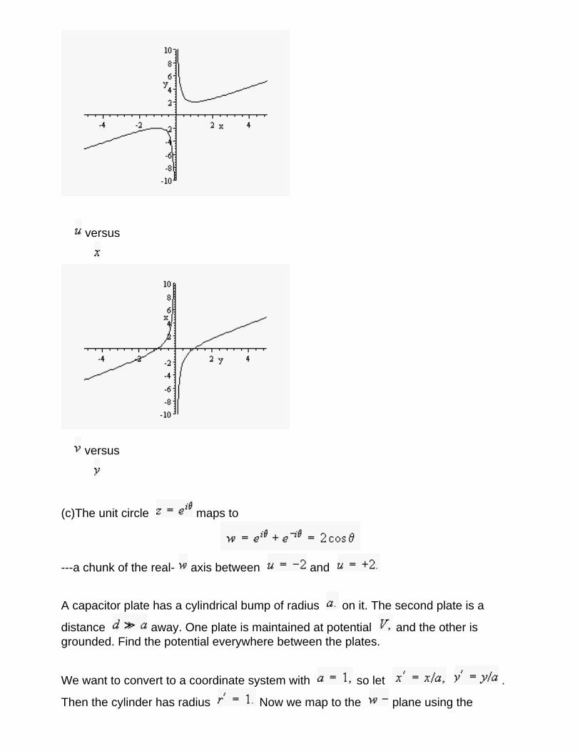
versus
versus
(c)The unit circle maps to
---a chunk of the real- axis between and
A capacitor plate has a cylindrical bump of radius on it. The second plate is a
distance away. One plate is maintained at potential and the other is grounded. Find the potential everywhere between the plates.
We want to convert to a coordinate system with so let .
Then the cylinder has radius Now we map to the plane using the
mapping This maps the cylinder plus axis to the axis. The second
plate has coordinate It maps to the line In this
plane the potential is
whic is zero for and for The complex potential is then:
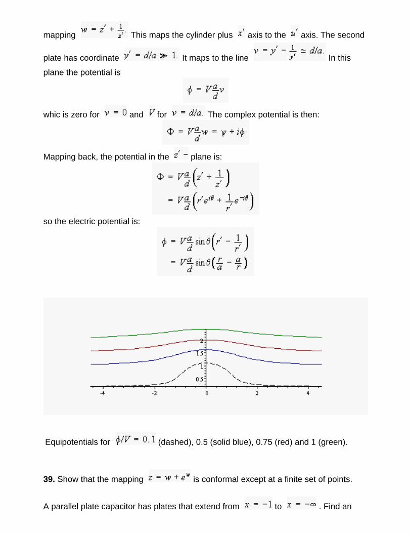
Mapping back, the potential in the plane is:
so the electric potential is:
Equipotentials for (dashed), 0.5 (solid blue), 0.75 (red) and 1 (green).
39. Show that the mapping is conformal except at a finite set of points.
A parallel plate capacitor has plates that extend from to . Find an
appropriate scaling that allows you to place the plates at Show that the given
transformation maps the plates to the lines Solve for the potential between
the plates in the plane, map to the plane and hence find the equipotential surfaces at the ends of the capacitor. Sketch the field lines. This is the so-called fringing field.
Choose where is a coordinate measured perpendicular to the plates, and
is the plate separation. The function is analytic everywhere, and the derivative is
It is non-zero except at the points
or, equivalently,
The mapping takes the form:
Then for ranges from to i.e. we
get the whole real axis in the plane. The line maps to
ranges from at to at This is the top
plate of the capacitor. Similarly maps to the lower plate.
The mapping has a branch point at each of the points
Each 2 wide strip of the plane maps to the whole
plane For each branch there are two points in the plane at which the mapping is not conformal.
In the plane we can write the potential as giving a complex potential
with the complex part being the physical potential. Equipotentials
correspond to const The corresponding curves in the plane are:
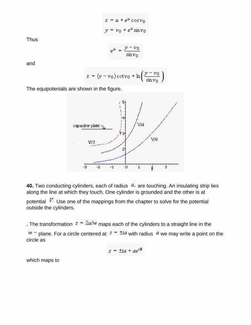
Thus
and
The equipotenials are shown in the figure.
40. Two conducting cylinders, each of radius are touching. An insulating strip lies along the line at which they touch. One cylinder is grounded and the other is at
potential Use one of the mappings from the chapter to solve for the potential outside the cylinders.
. The transformation maps each of the cylinders to a straight line in the
plane. For a circle centered at with radius we may write a point on the circle as
which maps to
As varies, takes on all real values and falls on the lines
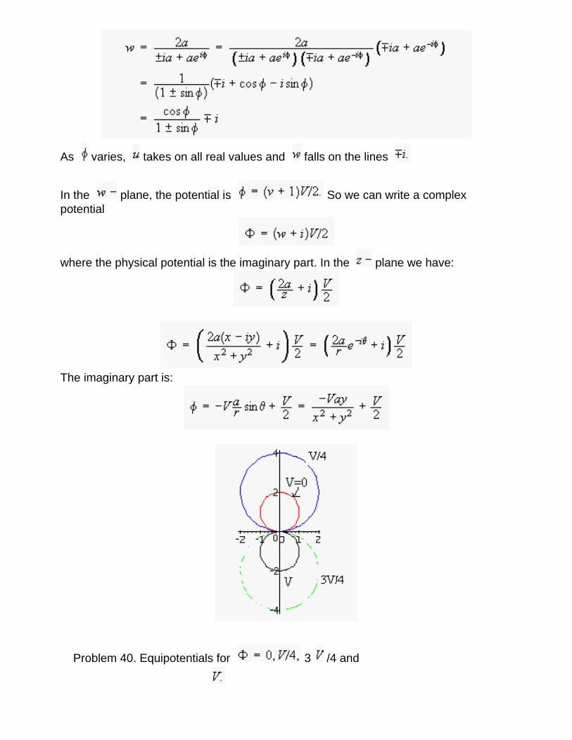
In the plane, the potential is So we can write a complex potential
where the physical potential is the imaginary part. In the plane we have:
The imaginary part is:
Problem 40. Equipotentials for 3 /4 and
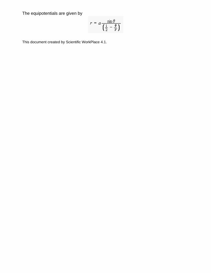
The equipotentials are given by
This document created by Scientific WorkPlace 4.1.
Chapter 2: Complex variables.
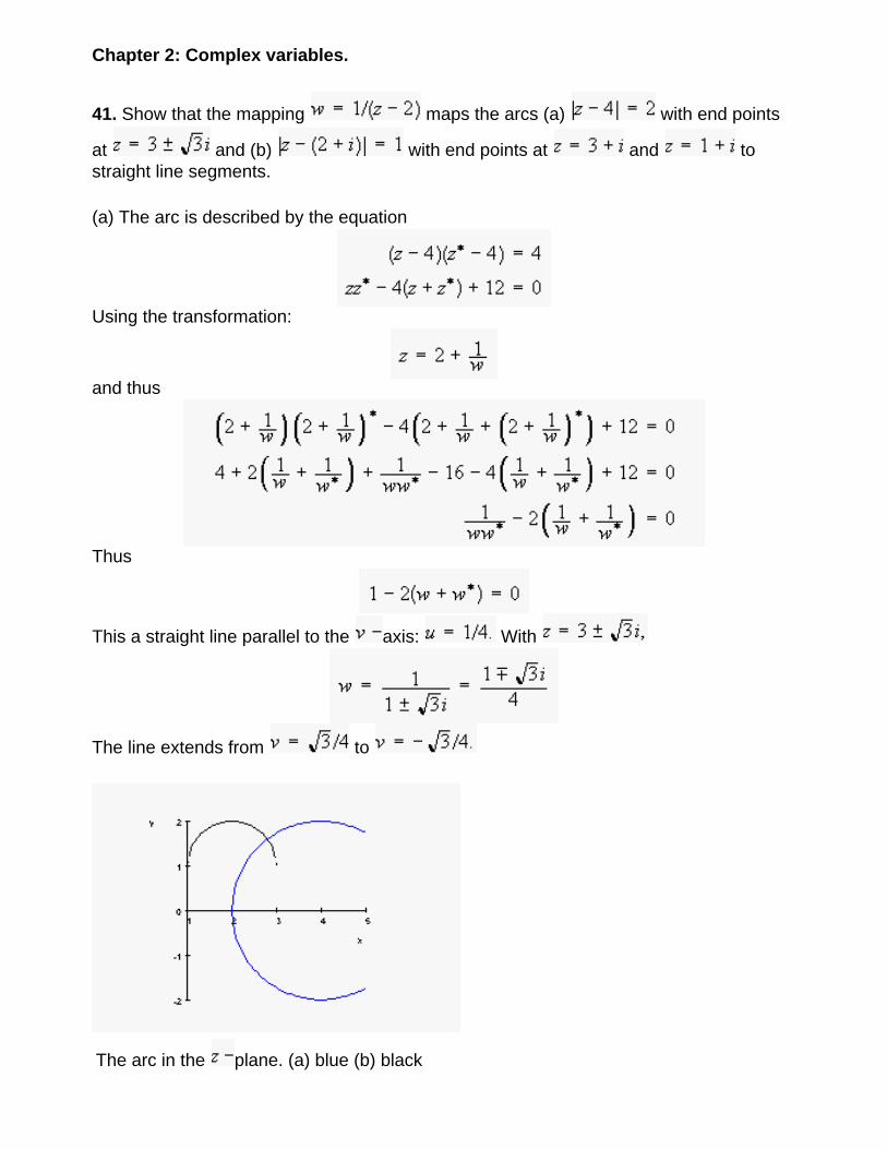
41. Show that the mapping maps the arcs (a) with end points
at and (b) with end points at and to straight line segments.
(a) The arc is described by the equation
Using the transformation:
and thus
Thus
This a straight line parallel to the axis: With
The line extends from to
The arc in the plane. (a) blue (b) black
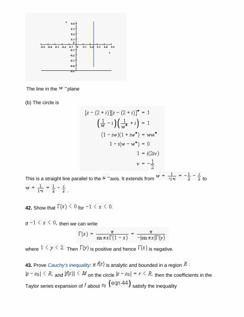
The line in the plane
(b) The circle is
This is a straight line parallel to the axis. It extends from to
.
42. Show that for
If then we can write
where Then is positive and hence is negative.
43. Prove Cauchy's inequality: If is analytic and bounded in a region
and on the circle then the coefficients in the
Taylor series expansion of about satisfy the inequality
Hence prove Liouville's theorem:
If is analytic and bounded in the entire complex plane, then it is a constant.
Using expression (45) with equal to the circle of radius
as required.
To Prove Liouville's theorem, we let and Then for all Thus
a constant.
44. A function is analytic except for well-separated simple poles at
Show that the function may be expanded in a series
where is the residue of at Is the result valid for Why or why not?
Hint: Evaluate the integral
where is a circle of radius about the origin that contains the poles. You may
assume that on for a small positive constant.
The integrand has simple poles at the origin, at and at Near one of the
poles the integrand has the form
The denominator of the first term has a simple zero at and the sum is analytic at
so the residue at is
Thus
But also
Thus as and so
as required.
The residue theorem holds when there are a finite number of poles inside the contour, so
this proof is limited to finite
See also Jeffreys and Jeffreys 11.175.
This document created by Scientific WorkPlace 4.1.
Chapter 3: Differential equations
1. A vehicle moves under the influence of a constant force and air resistance proportional to
velocity (equation 3.5 with replacing the gravitational force.) Find the speed of the vehicle as a
function of time if it starts from rest at
Choose axis along the direction of The equation of motion is then:
and the solution to the inhomogeneous equation is:
The solution to the homogeneous equation is of the form where
Thus the complete solution is of the form:
Now we apply the initial conditions:
So the solution is:
The vehicle reaches a terminal velocity as
2. Find the general solution to the differential equation
Hint: Extend the result for a double root from section 3.1.1.
The solution is of the form where
or a root repeated 3 times. Extending the result from the chapter, we guess that the two
additional solutions are and Let's check. With
and Substituting into the differential equation:
The coefficients of and are each zero, so this equation simplifies to which has solution
as expected. Thus the general solution is:
3. A capacitor inductor and resistor are connected in series with a switch. The capacitor
is charged by connecting it across a battery with emf The battery is disconnected, and the switch is closed. Find the current in the circuit as a function of time after the switch is closed.
The differential equation is:
and the intial condition is at The inductor prevents the current from changing
immediately after the switch is closed, so we also have at The solution is (§3.1.1)
with and Differentiating, we find
Applying the initial conditions, we have:
and
Thus
Notice that is negative for small implying that the capacitor is discharging.
4. The Airy differential equation is:
Find the two solutions of this equation as power series in
The point is a regular point of this equation, so we may write
and
Then the equation is
The lowest power that appears in this equation is and its coefficient is:
Then for we have:
and for
Thus the recursion relation skips two. One solution starts with
and the other starts with
5. Solve the equation (§3.3.2) using the Frobenius method. Show that cannot equal any non-zero constant, as discussed in §3.3.2.
The lowest power of is with coefficient
and solutions Then for we have
For
and for
The general recursion relation is:
Thus for
Thus the first solution is:
Check by differentiating
as required.
For
This generates the same solution as
This solution shows explicitly that the regular solution and const as Thus
cannot equal any non-zero constant, as discussed in the text.
The second solution is found using equation 3.37:
Differentiating:
Stuffing this into the differential equation, we get:
Using equation () our equation becomes:
The lowest power of in the first two terms is Thus must be an integer. With we find:
The coefficient of is:
The terms in are just again. Thus the general solution is:
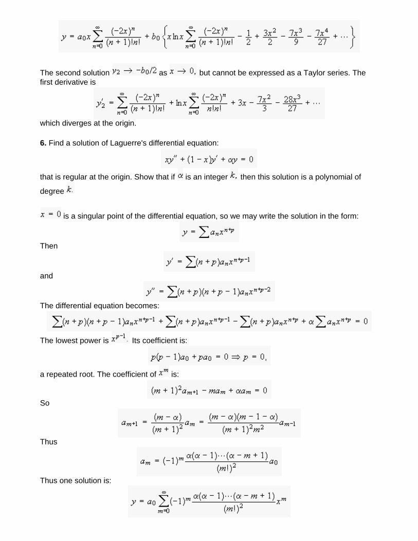
The second solution as but cannot be expressed as a Taylor series. The first derivative is
which diverges at the origin.
6. Find a solution of Laguerre's differential equation:
that is regular at the origin. Show that if is an integer then this solution is a polynomial of
degree
is a singular point of the differential equation, so we may write the solution in the form:
Then
and
The differential equation becomes:
The lowest power is Its coefficient is:
a repeated root. The coefficient of is:
So
Thus
Thus one solution is:
Now if an integer, then the series will terminate with and this solution becomes a
polynomial or order .
The first few are:
and so on.
The second solution is found by introducing the logarithm:
and inserting into the de.
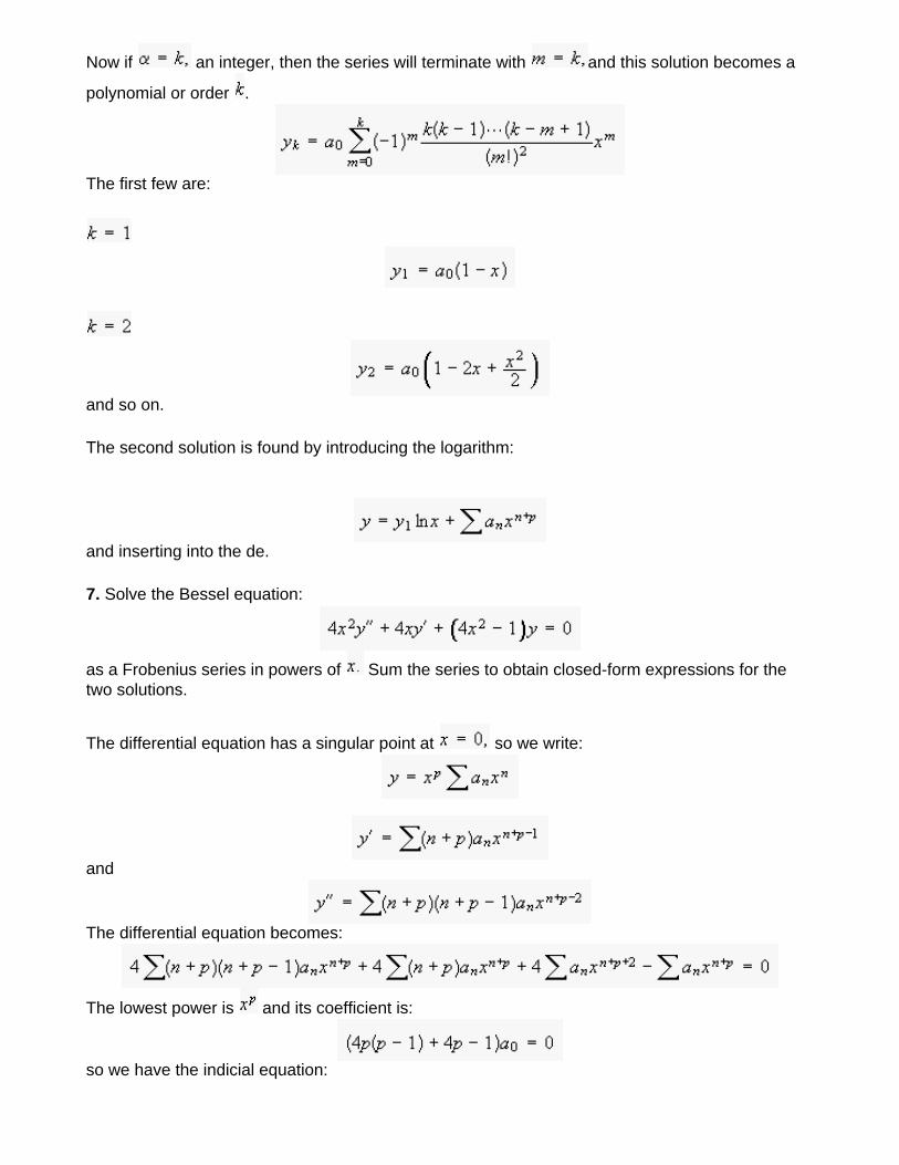
7. Solve the Bessel equation:
as a Frobenius series in powers of Sum the series to obtain closed-form expressions for the two solutions.
The differential equation has a singular point at so we write:
and
The differential equation becomes:
The lowest power is and its coefficient is:
so we have the indicial equation:
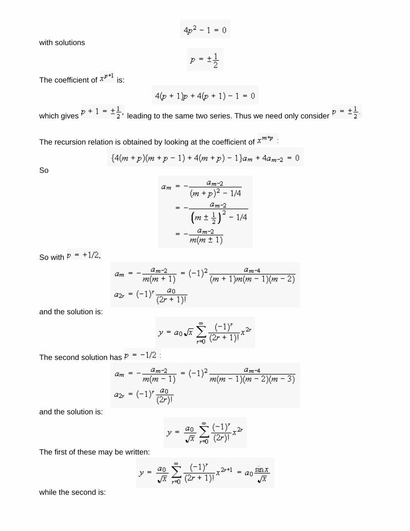
with solutions
The coefficient of is:
which gives leading to the same two series. Thus we need only consider
The recursion relation is obtained by looking at the coefficient of
So
So with
and the solution is:
The second solution has
and the solution is:
The first of these may be written:
while the second is:
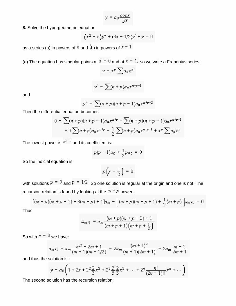
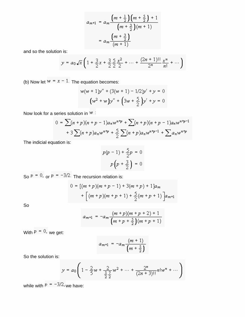
8. Solve the hypergeometric equation
as a series (a) in powers of and b) in powers of
(a) The equation has singular points at and at so we write a Frobenius series:
and
Then the differential equation becomes:
The lowest power is and its coefficient is:
So the indicial equation is
with solutions and So one solution is regular at the origin and one is not. The
recursion relation is found by looking at the power:
Thus
So with we have:
and thus the solution is:
The second solution has the recursion relation:
and so the solution is:
(b) Now let The equation becomes:
Now look for a series solution in
The indicial equation is:
So or The recursion relation is:
So
With we get:
So the solution is:
while with we have:
and the second solution is:
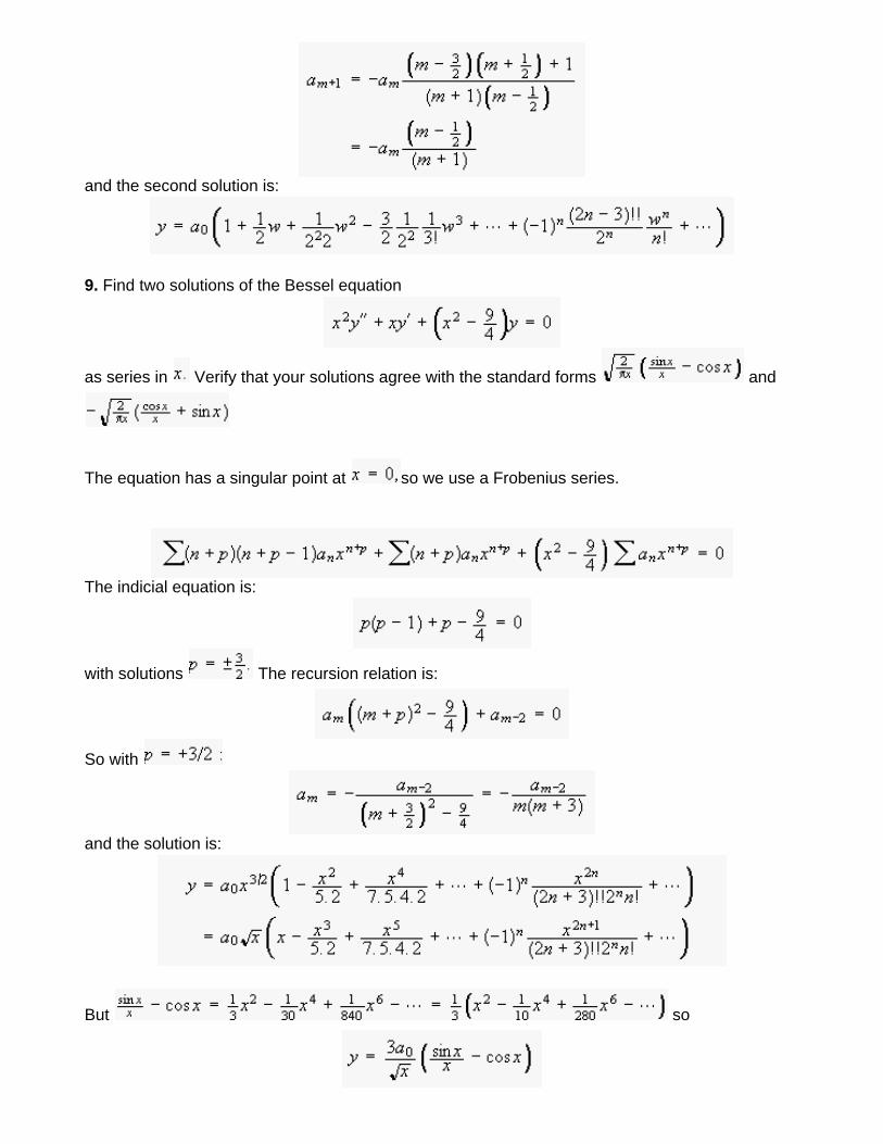
9. Find two solutions of the Bessel equation
as series in Verify that your solutions agree with the standard forms and
The equation has a singular point at so we use a Frobenius series.
The indicial equation is:
with solutions The recursion relation is:
So with
and the solution is:
But so
as required.
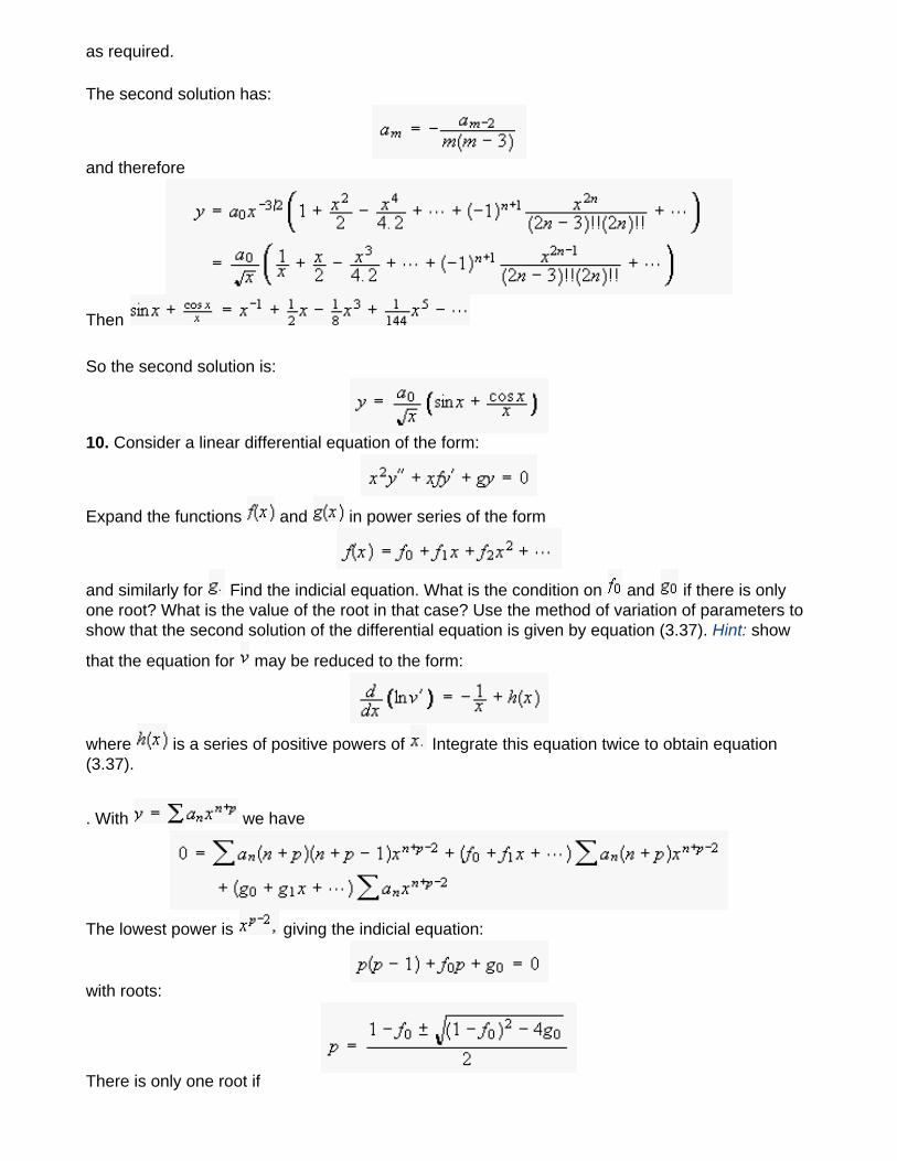
The second solution has:
and therefore
Then
So the second solution is:
10. Consider a linear differential equation of the form:
Expand the functions and in power series of the form
and similarly for Find the indicial equation. What is the condition on and if there is only one root? What is the value of the root in that case? Use the method of variation of parameters to show that the second solution of the differential equation is given by equation (3.37). Hint: show
that the equation for may be reduced to the form:
where is a series of positive powers of Integrate this equation twice to obtain equation (3.37).
. With we have
The lowest power is giving the indicial equation:
with roots:
There is only one root if
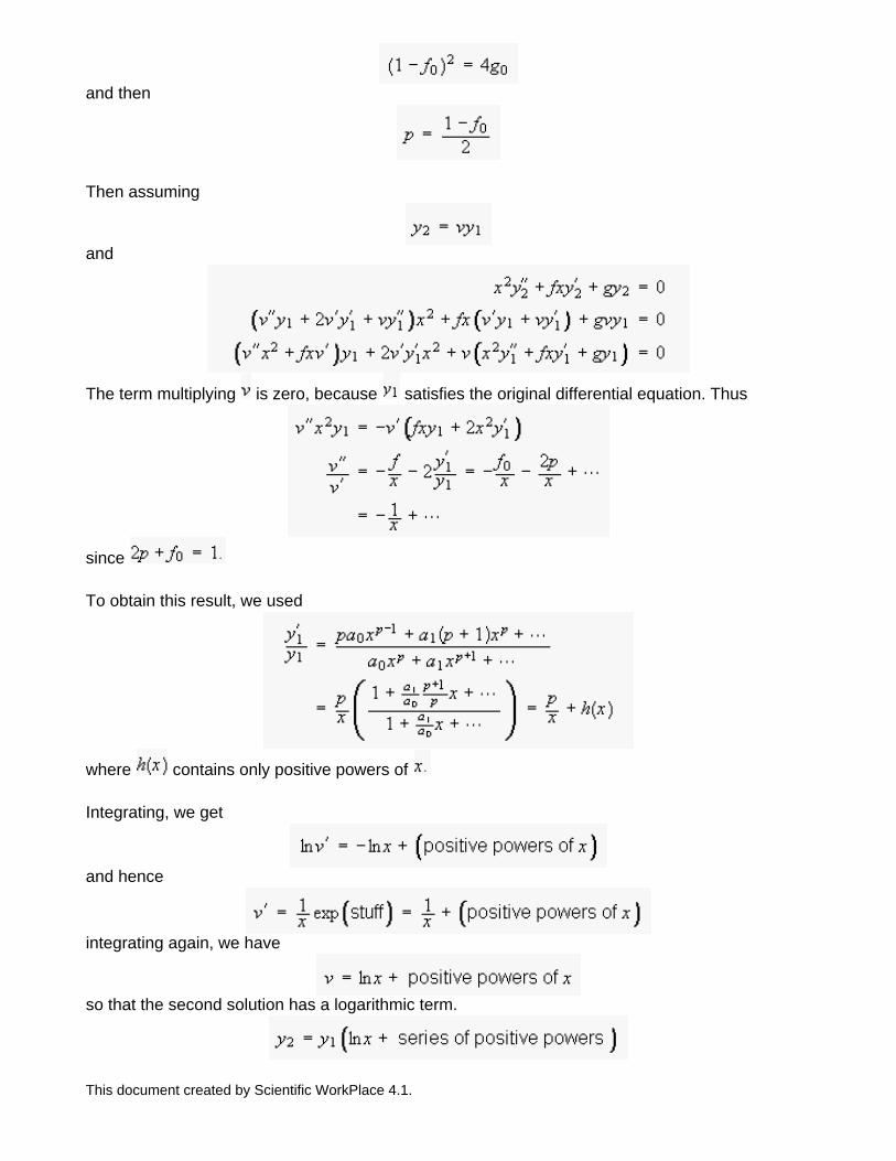
and then
Then assuming
and
The term multiplying is zero, because satisfies the original differential equation. Thus
since
To obtain this result, we used
where contains only positive powers of
Integrating, we get
and hence
integrating again, we have
so that the second solution has a logarithmic term.
This document created by Scientific WorkPlace 4.1.
Chapter 3: Differential equations
11. For a linear differential equation of the form where the functions and
are analytic, the indicial equation may be written as where is a quadratic
function. Show that in determining the recursion relation, the coefficient of the term is
Hence argue that the method fails to provide two solutions if the solutions of the equation differ by an integer.
First we insert the series into the differential equation:
To isolate the lowest power ( in this equation, we write the functions and using Taylor series about the origin: Then
Now we look at the power
The coefficient of is
Now if the solutions of are and then we will not be able to obtain a
solution for because its coefficient will be zero, and the method fails.
When does this argument fail? If the differential operator is even, then the
solution is purely even or purely odd. The recursion relation relates to If the roots of the indicial equation differ by unity, we will have two linearly independent solutions, one even solution and one odd solution, given by the two different roots.
12. Solve the equation (equation 3.19 in the chapter) by writing it in the form
and integrating twice.
13. Find the two solutions of the equation
The equation has a singular point at so we write a solution of the Frobenius type:
Then, multiplying by the differential equation becomes:
The lowest power that appears is and its coefficient is:
which has solutions . Inspection of the equation shows that is the complete
solution. Or, we can write the recursion relation by looking at the coefficient of
With we get:
So
if we start with we get an immediate problem, so we must conclude that and this is not a valid solution.
Starting with we get the recursion relation:
which gives and all succeeding terms zero. This is the solution that we guessed above.
For the second solution we choose a logarithm:
and
Stuffing into the differential equation, we have:
The lowest power is so we take
Then for the term we have:
For the term:
For the 2nd power:
and for the th power:
Then we can step down:
Thus the solution is:
14. Determine a solution of the equation
at large Hence determine the solution for all
At large the equation simplifies, since :
The solution is an exponential where
with only one solution, Thus at large
To determine the solution for all we look for a solution of the form Then:
and
and stuffing in, we get:
Since each term contains we cancel it:
Thus
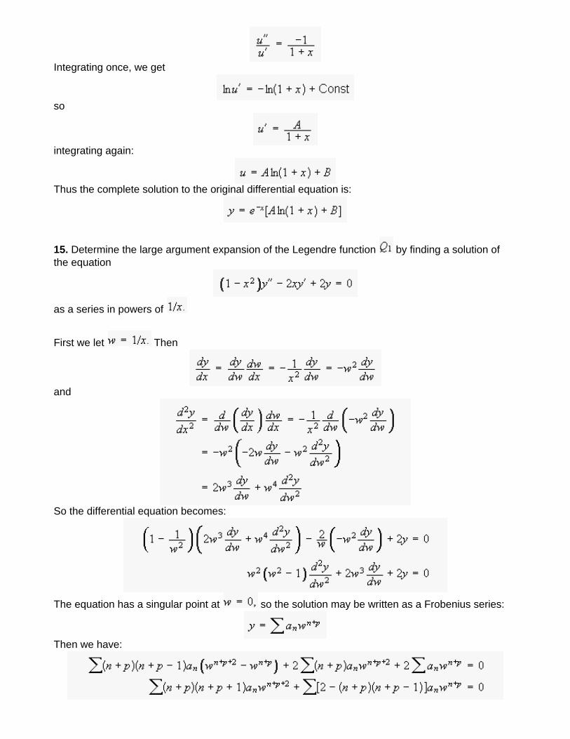
Integrating once, we get
so
integrating again:
Thus the complete solution to the original differential equation is:
15. Determine the large argument expansion of the Legendre function by finding a solution of the equation
as a series in powers of
First we let Then
and
So the differential equation becomes:
The equation has a singular point at so the solution may be written as a Frobenius series:
Then we have:
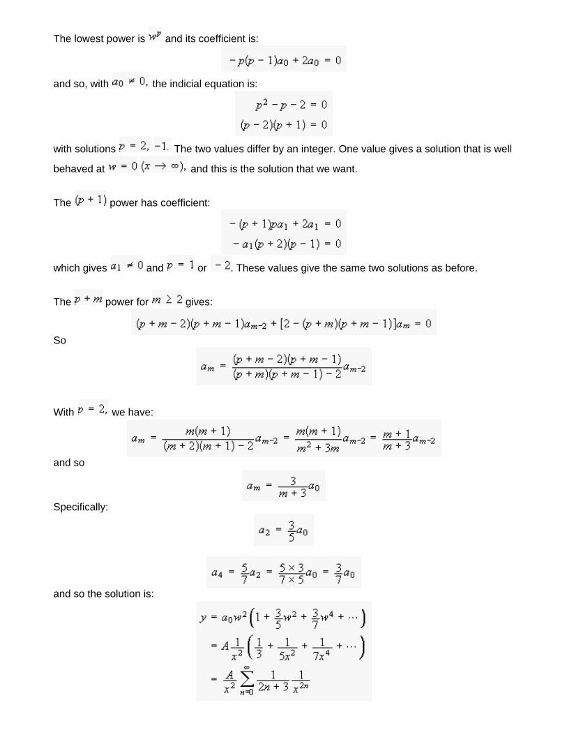
The lowest power is and its coefficient is:
and so, with the indicial equation is:
with solutions The two values differ by an integer. One value gives a solution that is well
behaved at and this is the solution that we want.
The power has coefficient:
which gives and or . These values give the same two solutions as before.
The power for gives:
So
With we have:
and so
Specifically:
and so the solution is:
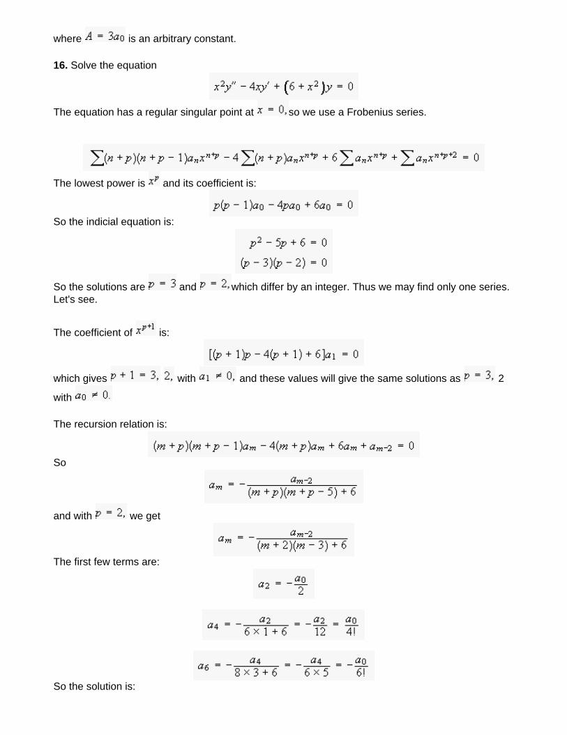
where is an arbitrary constant.
16. Solve the equation
The equation has a regular singular point at so we use a Frobenius series.
The lowest power is and its coefficient is:
So the indicial equation is:
So the solutions are and which differ by an integer. Thus we may find only one series. Let's see.
The coefficient of is:
which gives with and these values will give the same solutions as 2
with
The recursion relation is:
So
and with we get
The first few terms are:
So the solution is:
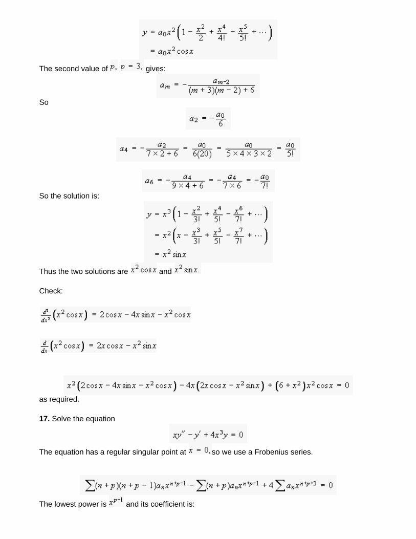
The second value of gives:
So
So the solution is:
Thus the two solutions are and
Check:
as required.
17. Solve the equation
The equation has a regular singular point at so we use a Frobenius series.
The lowest power is and its coefficient is:
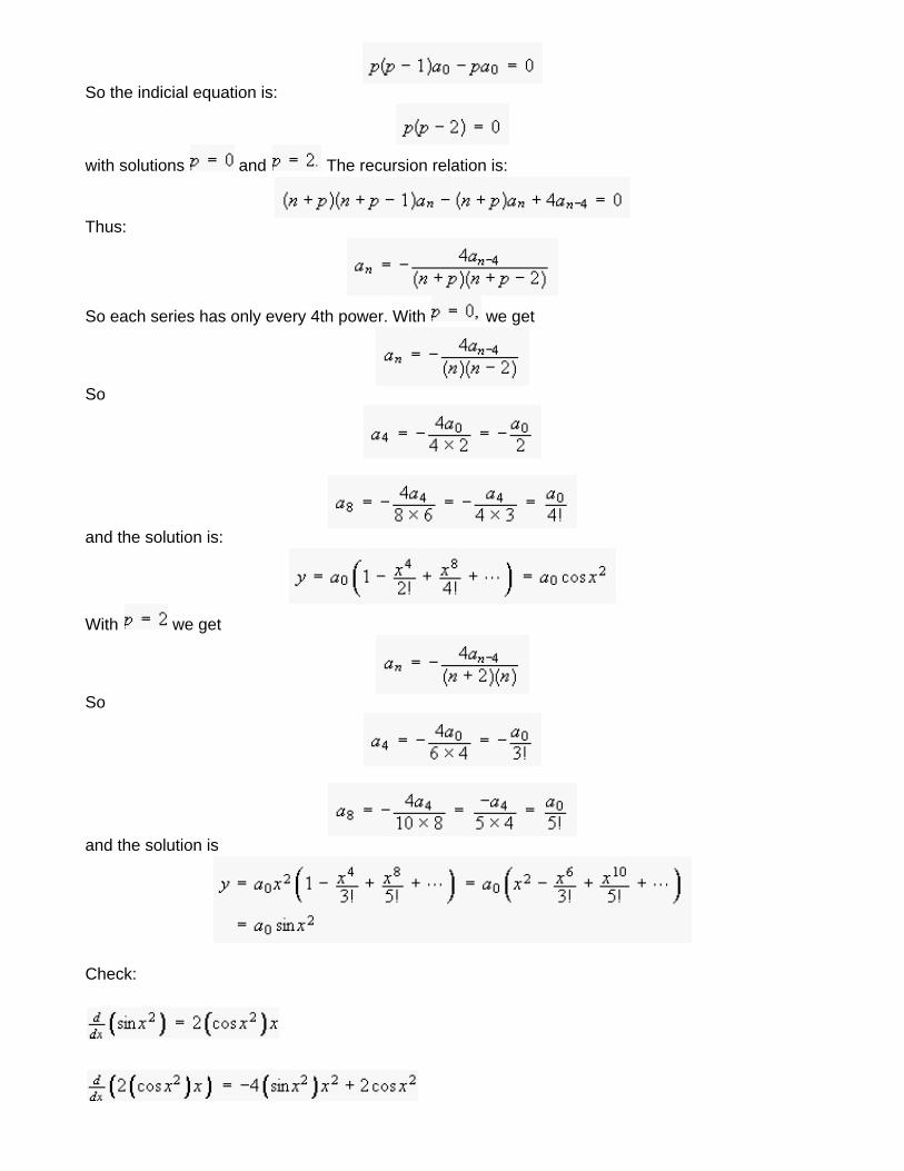
So the indicial equation is:
with solutions and The recursion relation is:
Thus:
So each series has only every 4th power. With we get
So
and the solution is:
With we get
So
and the solution is
Check:
as required.
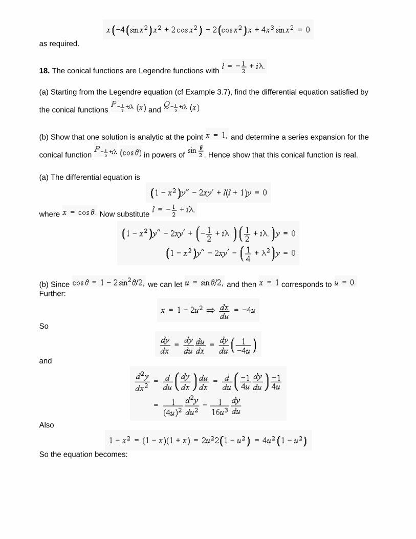
18. The conical functions are Legendre functions with
(a) Starting from the Legendre equation (cf Example 3.7), find the differential equation satisfied by
the conical functions and
(b) Show that one solution is analytic at the point and determine a series expansion for the
conical function in powers of . Hence show that this conical function is real.
(a) The differential equation is
where Now substitute
(b) Since we can let and then corresponds to Further:
So
and
Also
So the equation becomes:
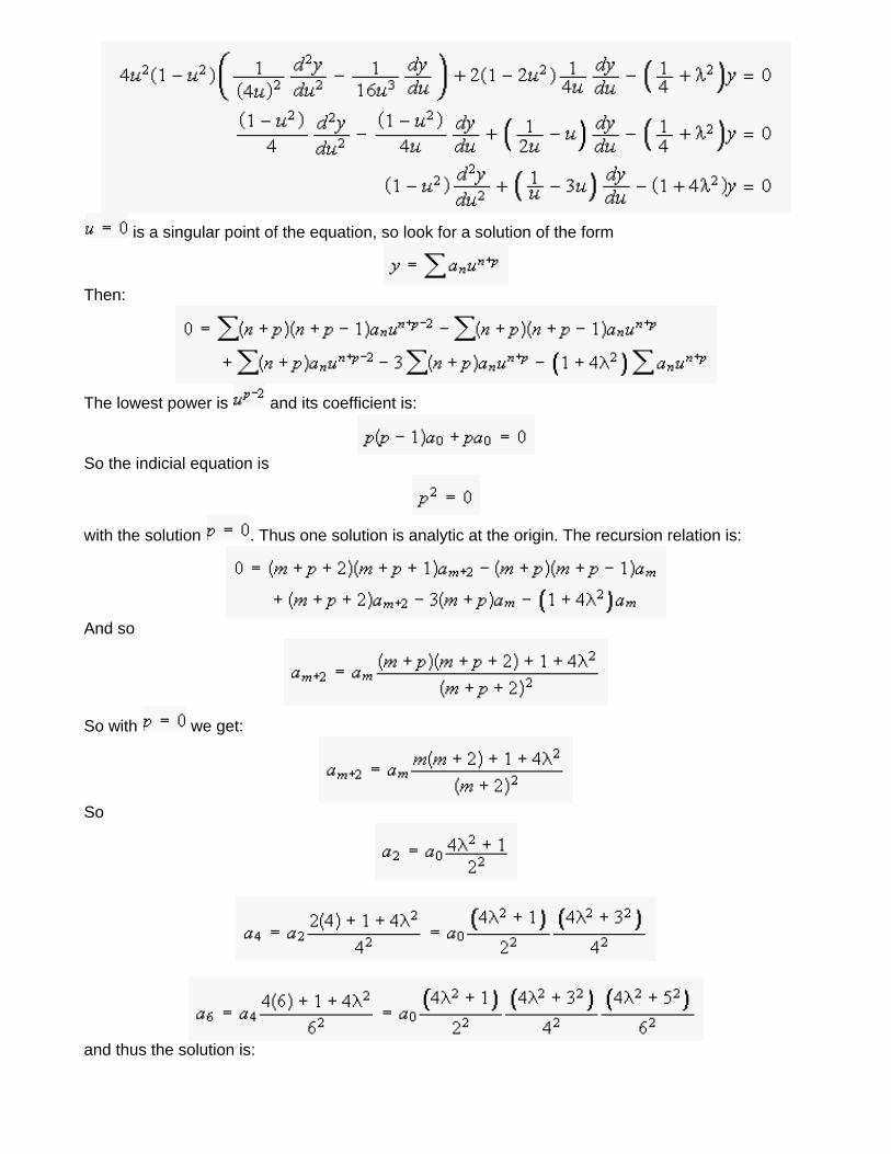
is a singular point of the equation, so look for a solution of the form
Then:
The lowest power is and its coefficient is:
So the indicial equation is
with the solution . Thus one solution is analytic at the origin. The recursion relation is:
And so
So with we get:
So
and thus the solution is:
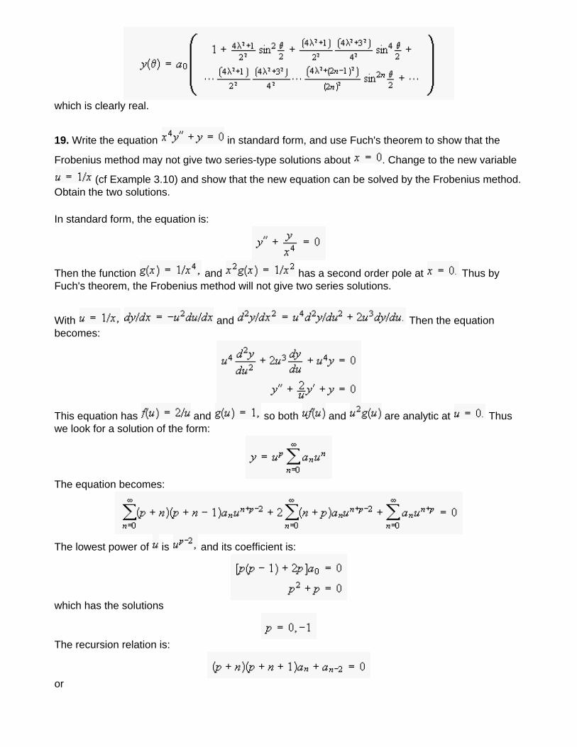
which is clearly real.
19. Write the equation in standard form, and use Fuch's theorem to show that the
Frobenius method may not give two series-type solutions about . Change to the new variable
(cf Example 3.10) and show that the new equation can be solved by the Frobenius method. Obtain the two solutions.
In standard form, the equation is:
Then the function and has a second order pole at Thus by Fuch's theorem, the Frobenius method will not give two series solutions.
With and Then the equation becomes:
This equation has and so both and are analytic at Thus we look for a solution of the form:
The equation becomes:
The lowest power of is and its coefficient is:
which has the solutions
The recursion relation is:
or
With
With
The recursion relation skips powers, so the series will have only even terms:
Thus the general solution is:
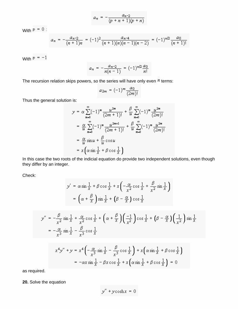
In this case the two roots of the indicial equation do provide two independent solutions, even though they differ by an integer.
Check:
as required.
20. Solve the equation
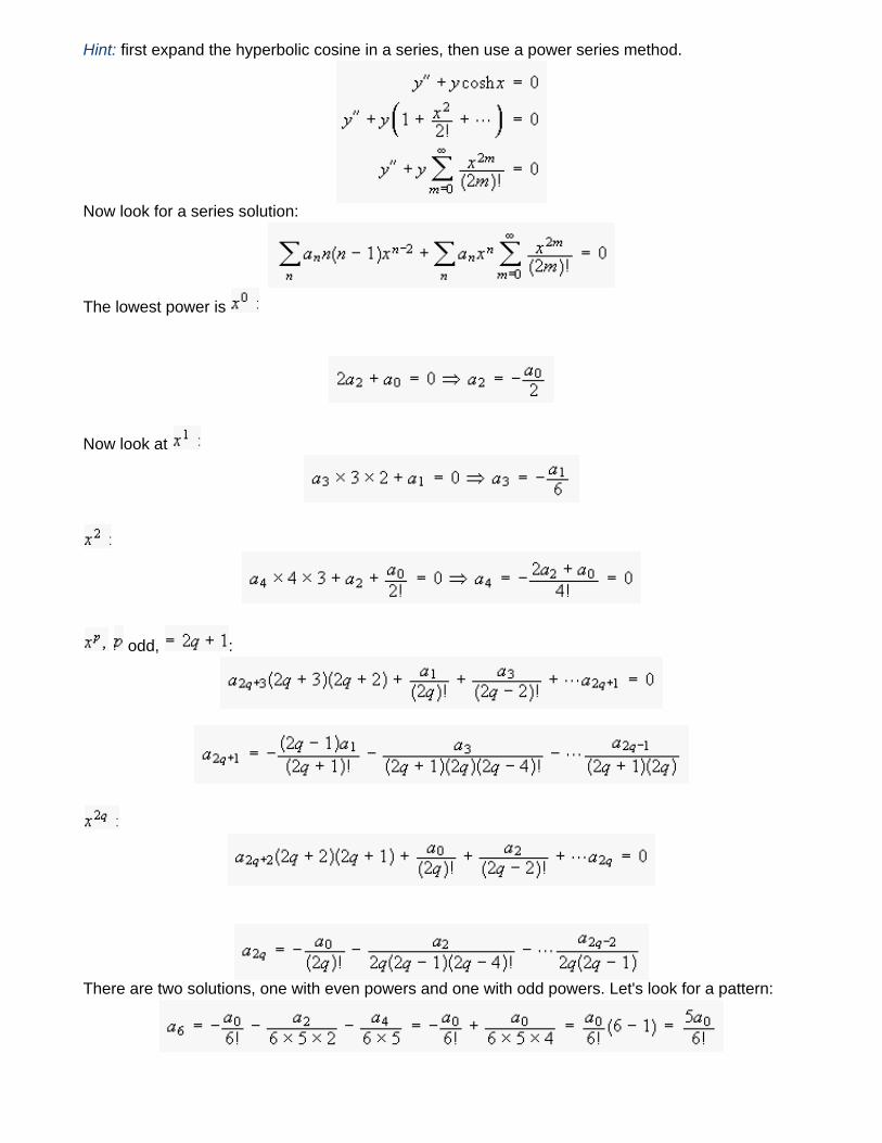
Hint: first expand the hyperbolic cosine in a series, then use a power series method.
Now look for a series solution:
The lowest power is
Now look at
odd, :
There are two solutions, one with even powers and one with odd powers. Let's look for a pattern:
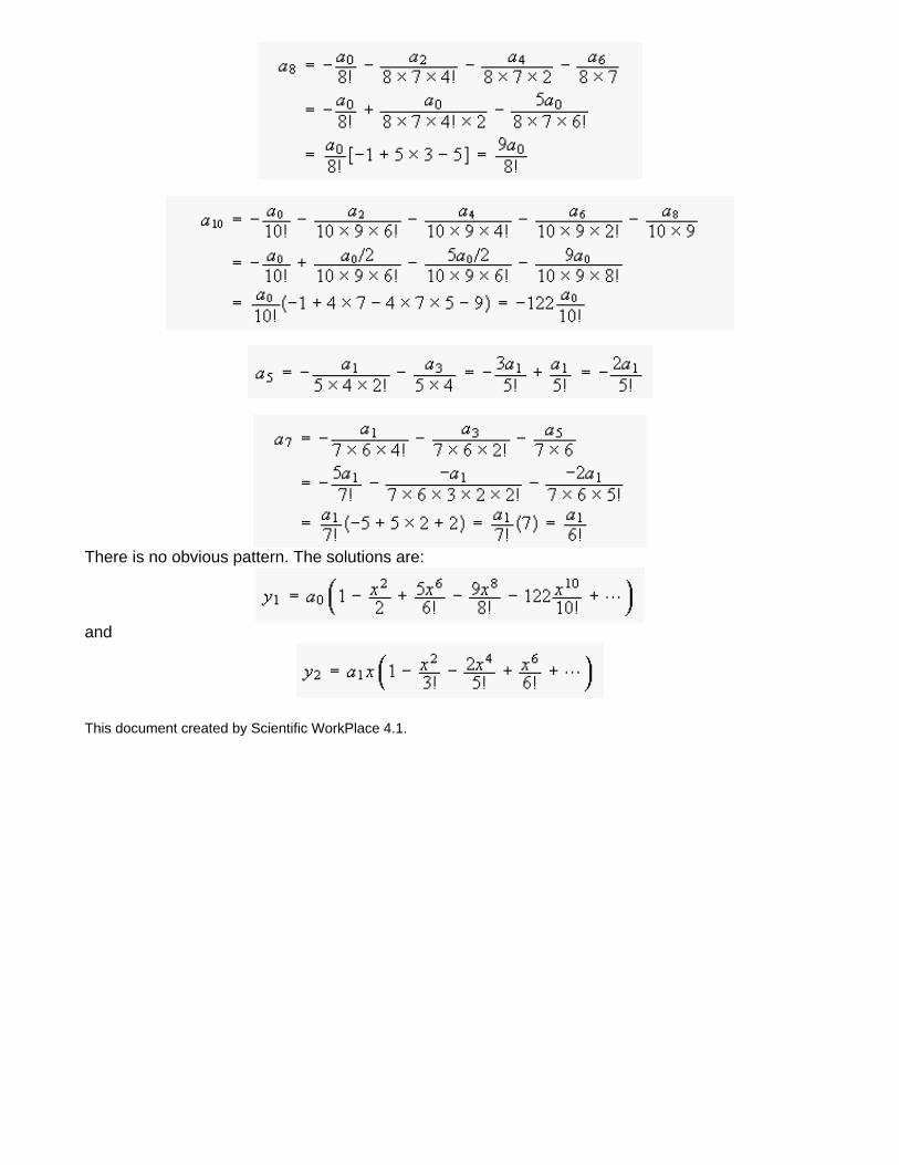
There is no obvious pattern. The solutions are:
and
This document created by Scientific WorkPlace 4.1.
Chapter 3: Differential equations
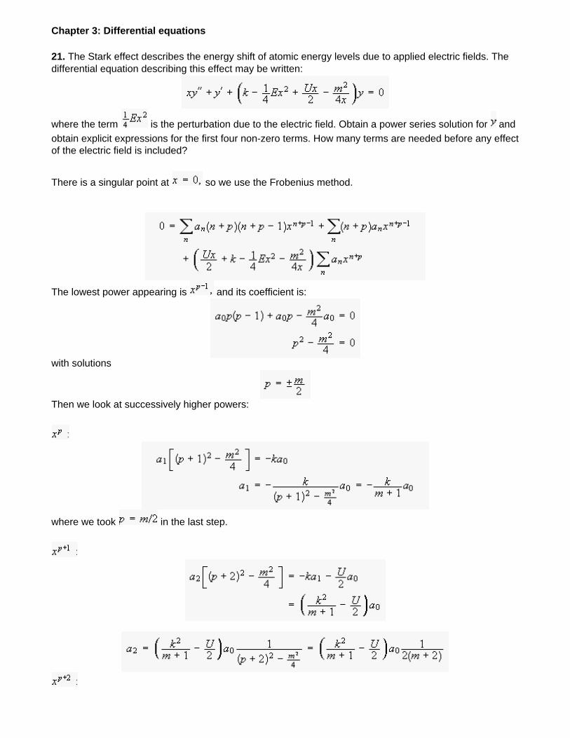
21. The Stark effect describes the energy shift of atomic energy levels due to applied electric fields. The differential equation describing this effect may be written:
where the term is the perturbation due to the electric field. Obtain a power series solution for and obtain explicit expressions for the first four non-zero terms. How many terms are needed before any effect of the electric field is included?
There is a singular point at so we use the Frobenius method.
The lowest power appearing is and its coefficient is:
with solutions
Then we look at successively higher powers:
where we took in the last step.
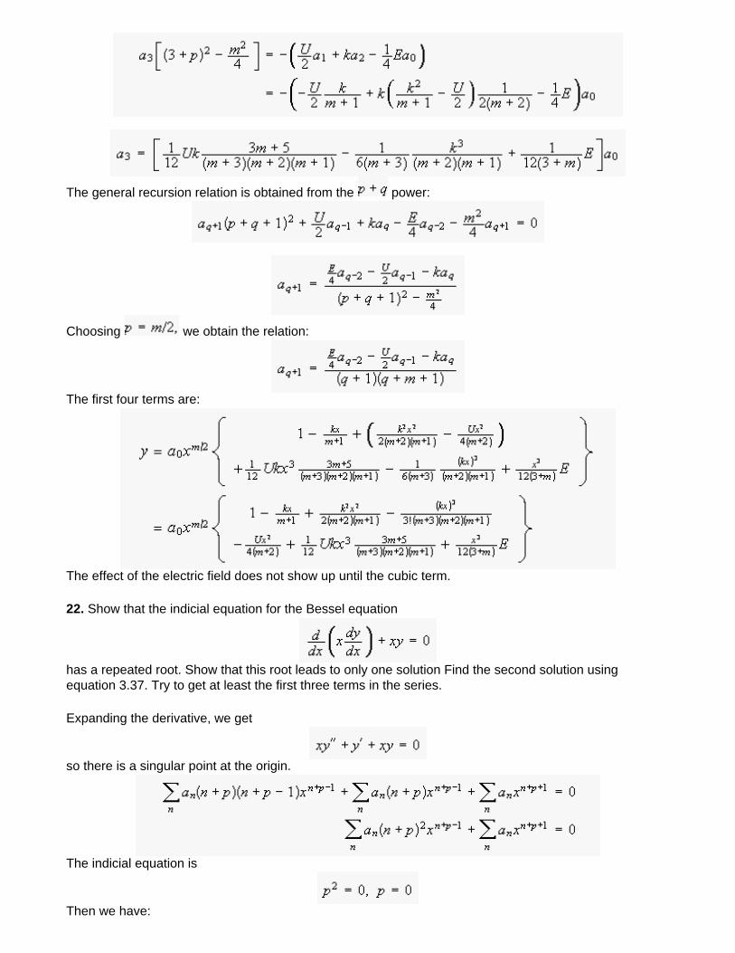
The general recursion relation is obtained from the power:
Choosing we obtain the relation:
The first four terms are:
The effect of the electric field does not show up until the cubic term.
22. Show that the indicial equation for the Bessel equation
has a repeated root. Show that this root leads to only one solution Find the second solution using equation 3.37. Try to get at least the first three terms in the series.
Expanding the derivative, we get
so there is a singular point at the origin.
The indicial equation is
Then we have:
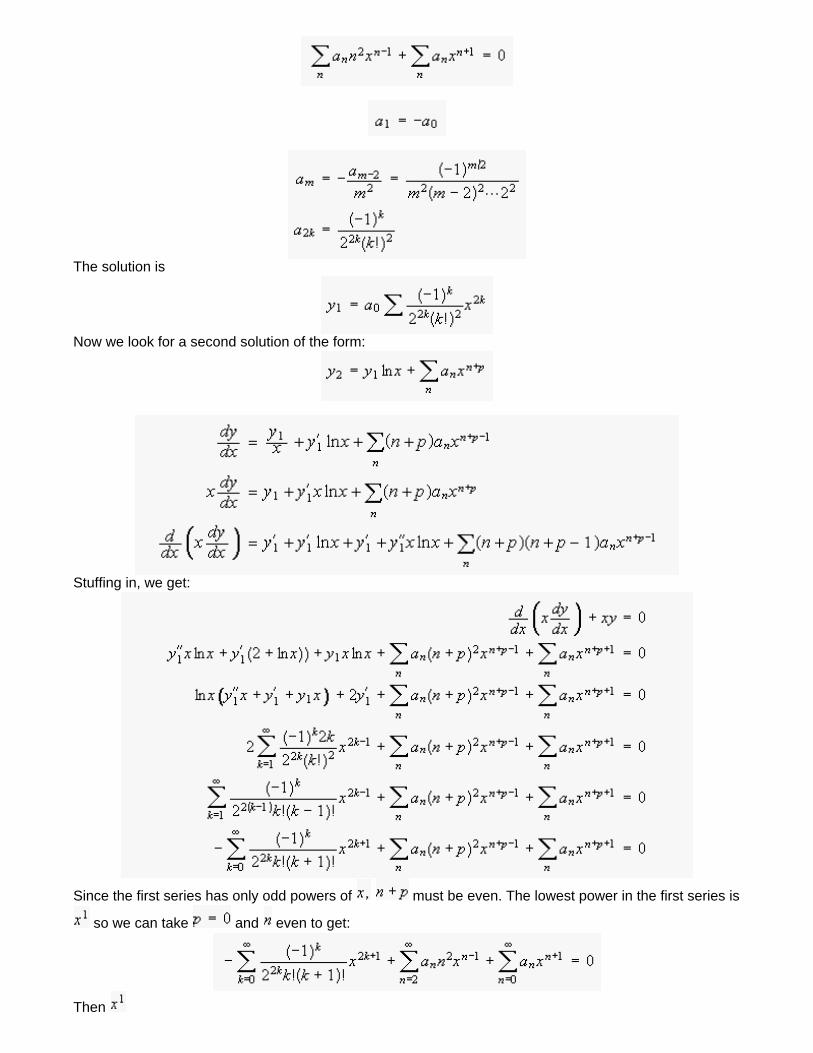
The solution is
Now we look for a second solution of the form:
Stuffing in, we get:
Since the first series has only odd powers of must be even. The lowest power in the first series is
so we can take and even to get:
Then
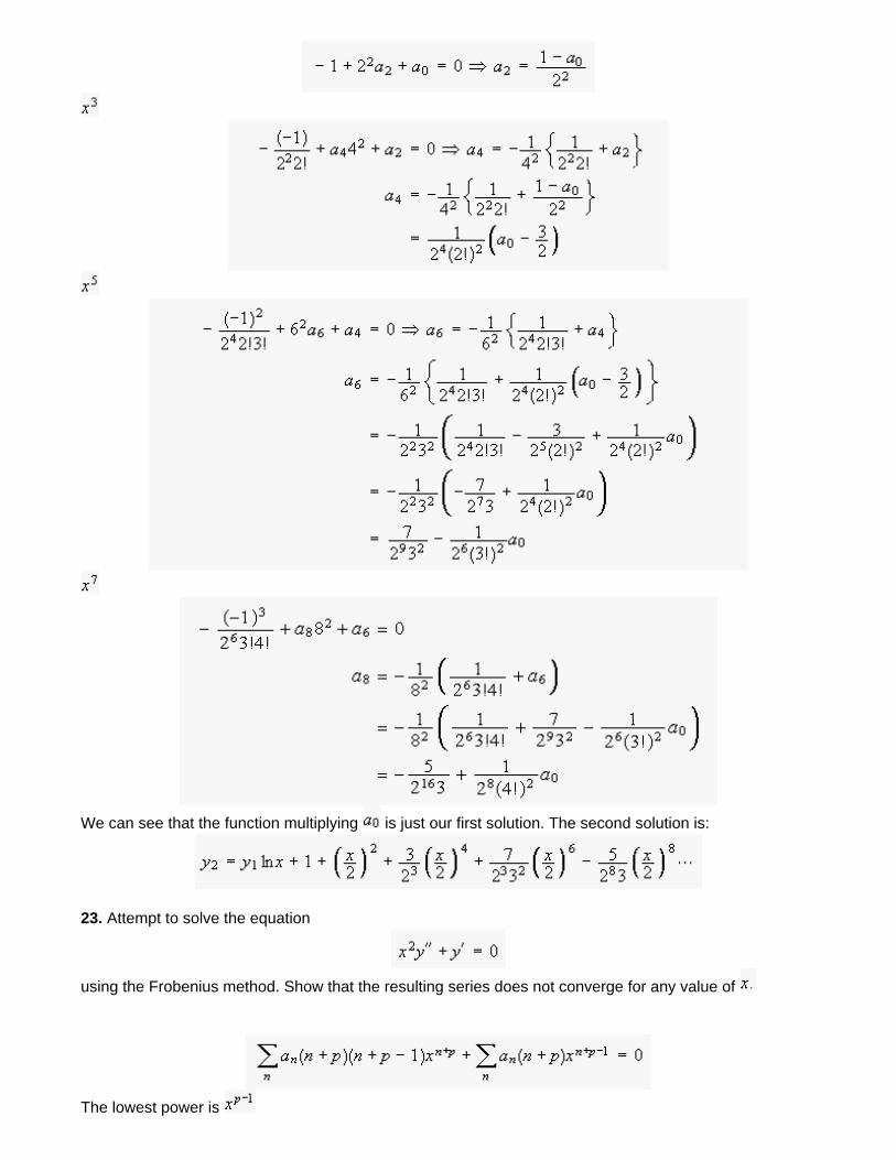
We can see that the function multiplying is just our first solution. The second solution is:
23. Attempt to solve the equation
using the Frobenius method. Show that the resulting series does not converge for any value of
The lowest power is
Thus we need or The next power is
With we get
The general recursion relation is:
From the ratio test, the ratio of two successive terms is
This ratio is for any finite value of for and thus the series diverges.
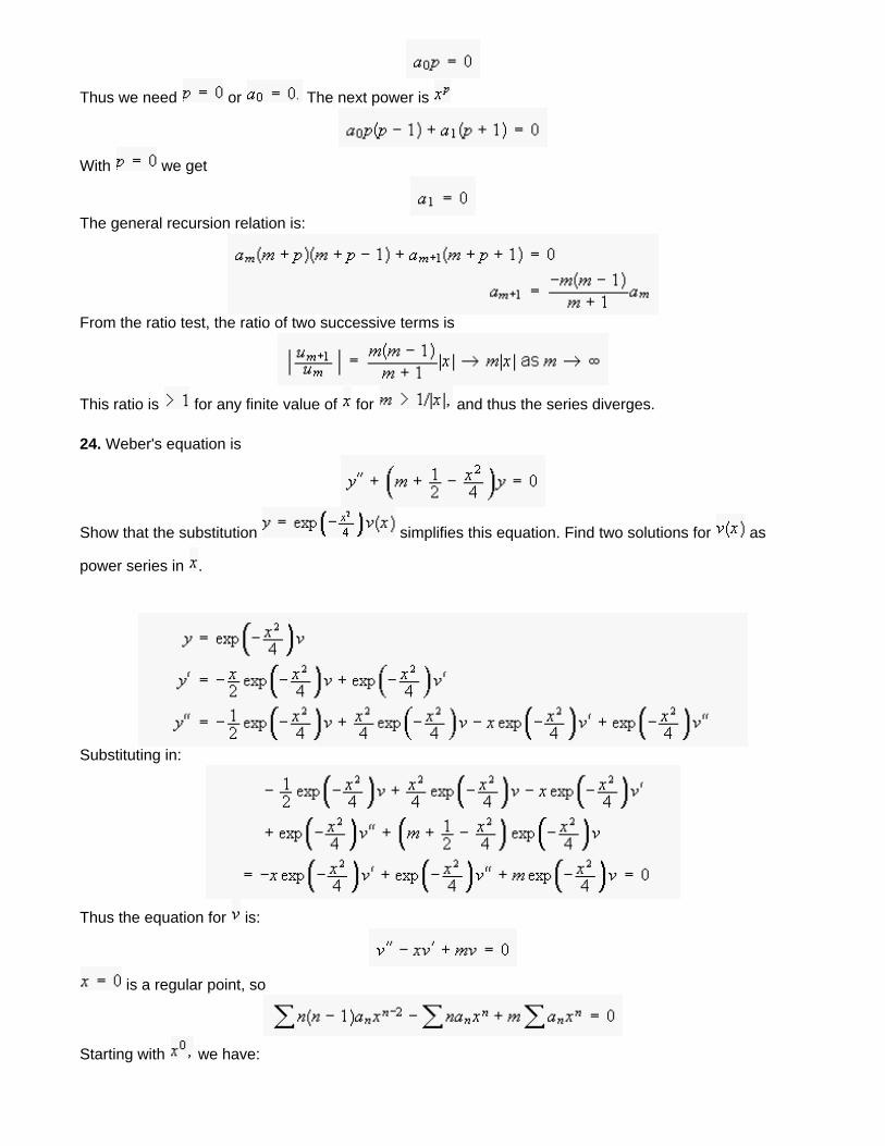
24. Weber's equation is
Show that the substitution simplifies this equation. Find two solutions for as
power series in .
Substituting in:
Thus the equation for is:
is a regular point, so
Starting with we have:
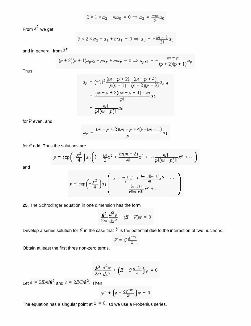
From we get
and in general, from
Thus
for even, and
for odd. Thus the solutions are
and
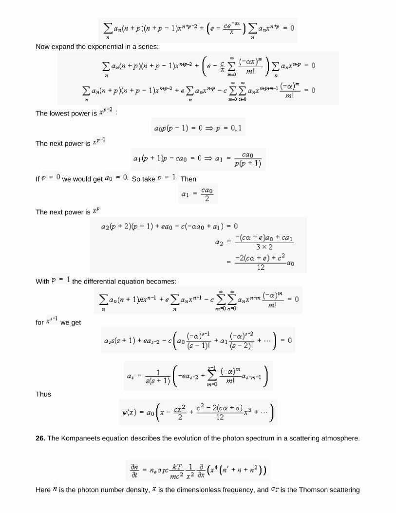
25. The Schrödinger equation in one dimension has the form
Develop a series solution for in the case that is the potential due to the interaction of two nucleons:
Obtain at least the first three non-zero terms.
Let and Then
The equation has a singular point at so we use a Frobenius series.
Now expand the exponential in a series:
The lowest power is
The next power is
If we would get So take Then
The next power is
With the differential equation becomes:
for we get
Thus
26. The Kompaneets equation describes the evolution of the photon spectrum in a scattering atmosphere.
Here is the photon number density, is the dimensionless frequency, and is the Thomson scattering
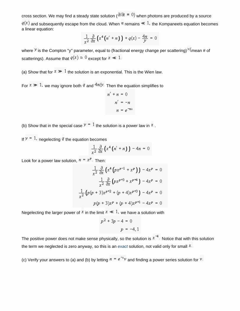
cross section. We may find a steady state solution ( when photons are produced by a source
and subsequently escape from the cloud. When remains the Kompaneets equation becomes a linear equation:
where is the Compton ''y'' parameter, equal to (fractional energy change per scattering) mean # of
scatterings). Assume that except for
(a) Show that for the solution is an exponential. This is the Wien law.
For we may ignore both and Then the equation simplifies to
(b) Show that in the special case the solution is a power law in .
If negelecting the equation becomes
Look for a power law solution, Then:
Negelecting the larger power of in the limit we have a solution with
The positive power does not make sense physically, so the solution is Notice that with this solution
the term we neglected is zero anyway, so this is an exact solution, not valid only for small
(c) Verify your answers to (a) and (b) by letting and finding a power series solution for
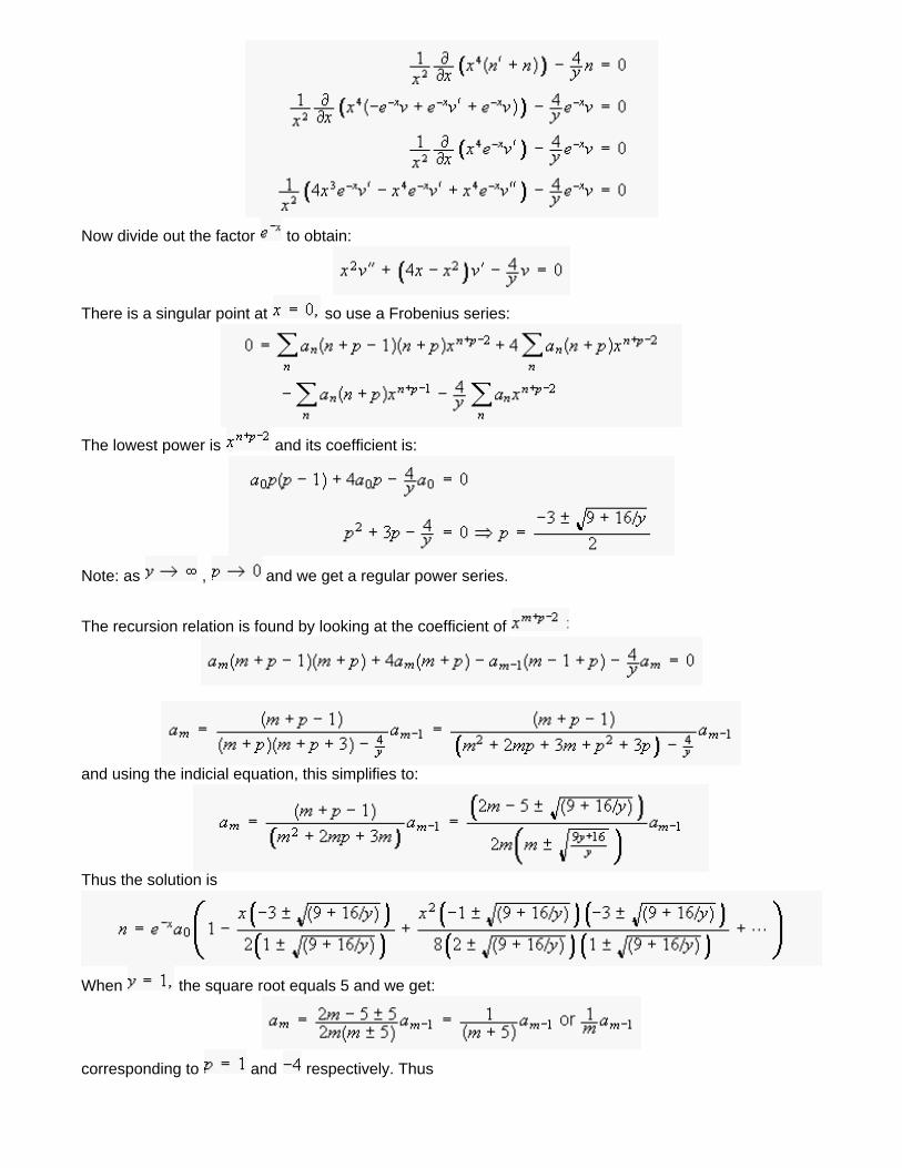
Now divide out the factor to obtain:
There is a singular point at so use a Frobenius series:
The lowest power is and its coefficient is:
Note: as , and we get a regular power series.
The recursion relation is found by looking at the coefficient of
and using the indicial equation, this simplifies to:
Thus the solution is
When the square root equals 5 and we get:
corresponding to and respectively. Thus
as we found in (b), or
27. A particle falls a distance under gravity. Air resistance is proportional to the square of the particle's speed. Write the differential equation that describes the particle's position as a function of time.
We start with Newton's 2nd law:
Choose dimensionless variables, and show that the equation may be put into the form:
Divide by
Each term in this equation is dimensionless. Express the distance travelled as a fraction of the total
distance and define a dimensionless time Then the equation becomes:
which is of the desired form with and Using a spreadsheet to compute the coordinates,
starting at we reach at corresponding to s. With no air resistance we would have:
Air resistance increases the time by 0.02 s or
With an increase of
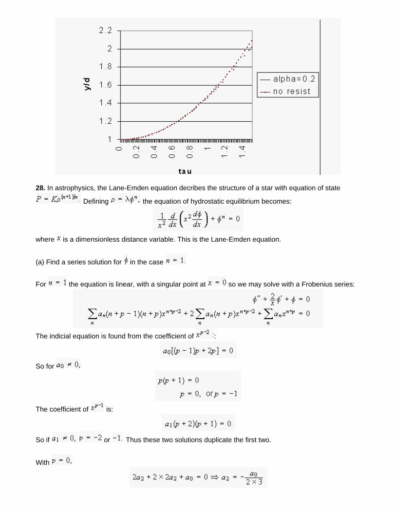
28. In astrophysics, the Lane-Emden equation decribes the structure of a star with equation of state
Defining the equation of hydrostatic equilibrium becomes:
where is a dimensionless distance variable. This is the Lane-Emden equation.
(a) Find a series solution for in the case
For the equation is linear, with a singular point at so we may solve with a Frobenius series:
The indicial equation is found from the coefficient of :
So for
The coefficient of is:
So if or Thus these two solutions duplicate the first two.
With
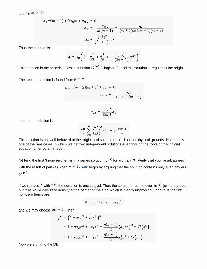
and for
Thus the solution is
This function is the spherical Bessel function (Chapter 8), and this solution is regular at the origin.
The second solution is found from
and so the solution is
This solution is not well behaved at the origin, and so can be ruled out on physical grounds. Note this is one of the rare cases in which we get two independent solutions even though the roots of the indicial equation differ by an integer.
(b) Find the first 3 non-zero terms in a series solution for for arbitrary Verify that your result agrees
with the result of part (a) when (Hint: begin by arguing that the solution contains only even powers
of
If we replace with the equation is unchanged. Thus the solution must be even in (or purely odd, but that would give zero density at the center of the star, which is clearly unphysical), and thus the first 3 non-zero terms are:
and we may choose Then
Now we stuff into the DE
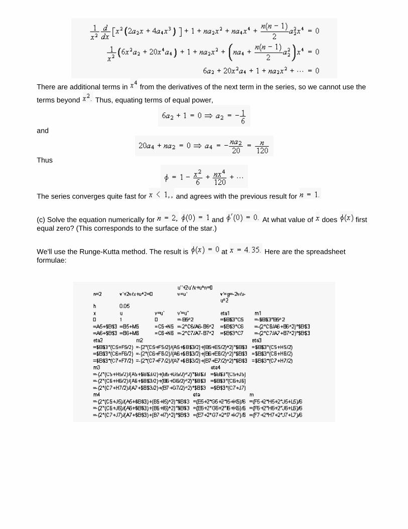
There are additional terms in from the derivatives of the next term in the series, so we cannot use the
terms beyond Thus, equating terms of equal power,
and
Thus
The series converges quite fast for and agrees with the previous result for
(c) Solve the equation numerically for and At what value of does first equal zero? (This corresponds to the surface of the star.)
We'll use the Runge-Kutta method. The result is at Here are the spreadsheet formulae:
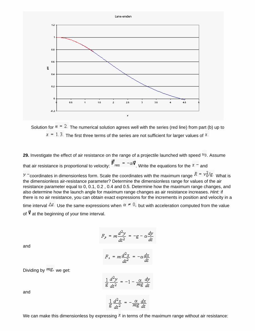
Solution for The numerical solution agrees well with the series (red line) from part (b) up to
The first three terms of the series are not sufficient for larger values of
29. Investigate the effect of air resistance on the range of a projectile launched with speed . Assume
that air resistance is proportional to velocity: . Write the equations for the and
coordinates in dimensionless form. Scale the coordinates with the maximum range What is the dimensionless air-resistance parameter? Determine the dimensionless range for values of the air resistance parameter equal to 0, 0.1, 0.2 , 0.4 and 0.5. Determine how the maximum range changes, and also determine how the launch angle for maximum range changes as air resistance increases. Hint: if there is no air resistance, you can obtain exact expressions for the increments in position and velocity in a
time interval Use the same expressions when but with acceleration computed from the value
of at the beginning of your time interval.
and
Dividing by we get:
and
We can make this dimensionless by expressing in terms of the maximum range without air resistance:
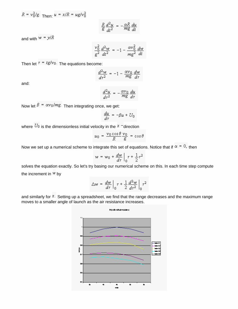
Then:
and with
Then let The equations become:
and:
Now let Then integrating once, we get:
where is the dimensionless initial velocity in the direction
Now we set up a numerical scheme to integrate this set of equations. Notice that if then
solves the equation exactly. So let's try basing our numerical scheme on this. In each time step compute
the increment in by
and similarly for Setting up a spreadsheet, we find that the range decreases and the maximum range moves to a smaller angle of launch as the air resistance increases.
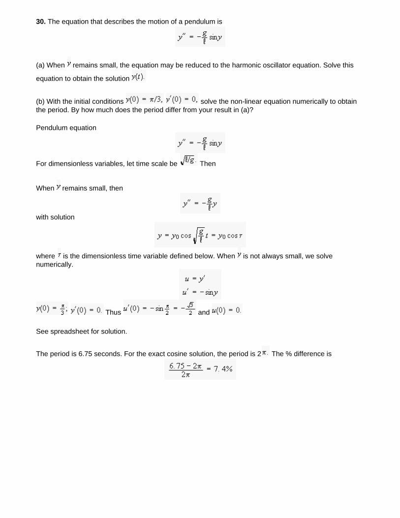
30. The equation that describes the motion of a pendulum is
(a) When remains small, the equation may be reduced to the harmonic oscillator equation. Solve this
equation to obtain the solution
(b) With the initial conditions solve the non-linear equation numerically to obtain the period. By how much does the period differ from your result in (a)?
Pendulum equation
For dimensionless variables, let time scale be Then
When remains small, then
with solution
where is the dimensionless time variable defined below. When is not always small, we solve numerically.
Thus and
See spreadsheet for solution.
The period is 6.75 seconds. For the exact cosine solution, the period is 2 The % difference is
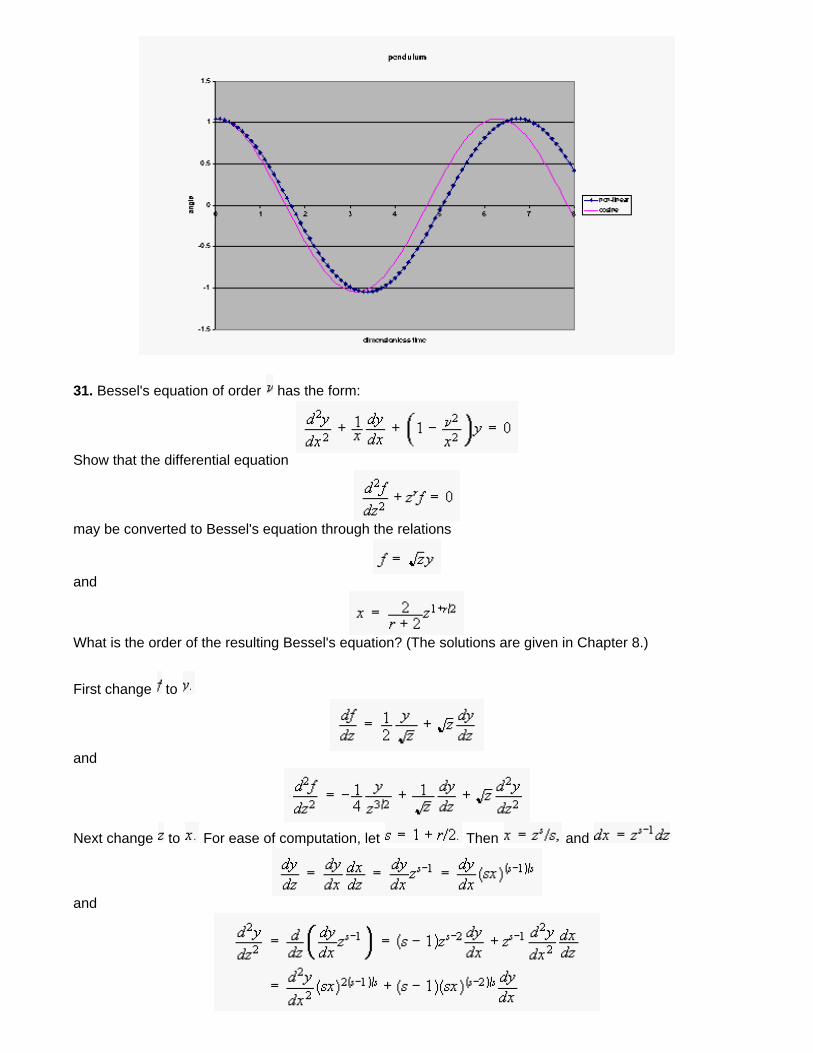
31. Bessel's equation of order has the form:
Show that the differential equation
may be converted to Bessel's equation through the relations
and
What is the order of the resulting Bessel's equation? (The solutions are given in Chapter 8.)
First change to
and
Next change to For ease of computation, let Then and
and
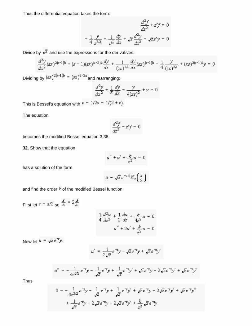
Thus the differential equation takes the form:
Divide by and use the expressions for the derivatives:
Dividing by and rearranging:
This is Bessel's equation with
The equation
becomes the modified Bessel equation 3.38.
32. Show that the equation
has a solution of the form
and find the order of the modified Bessel function.
First let so
Now let
Thus
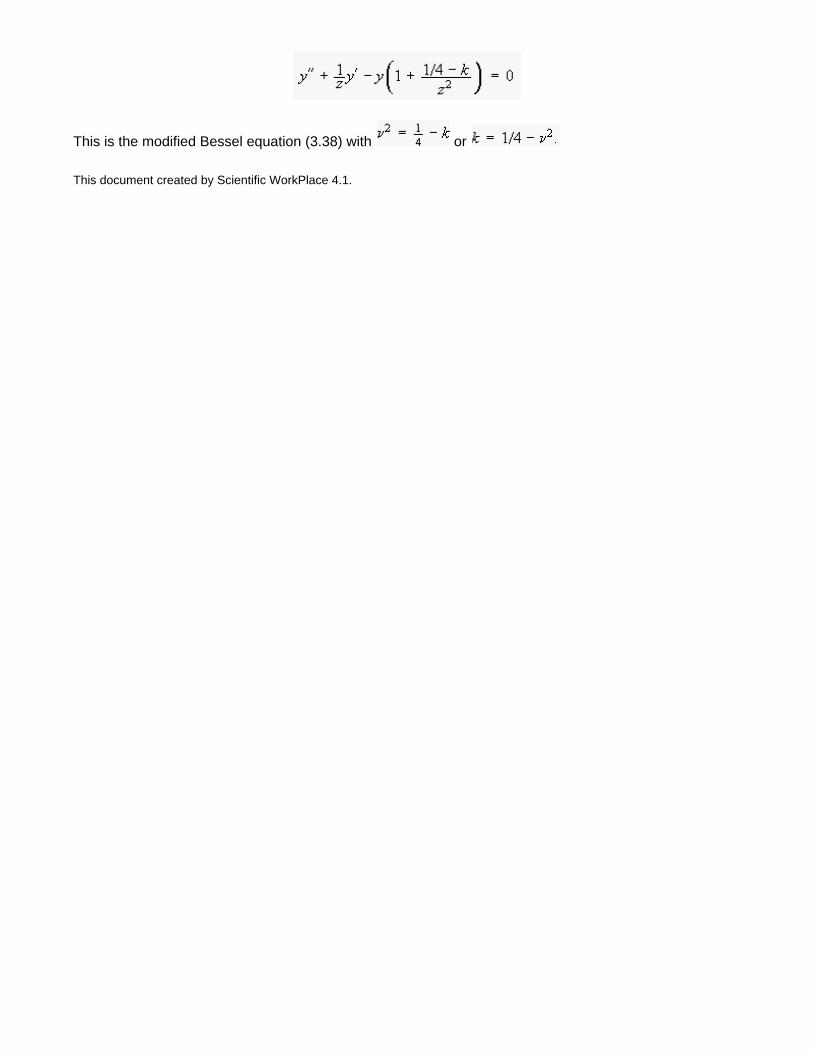
This is the modified Bessel equation (3.38) with or
This document created by Scientific WorkPlace 4.1.
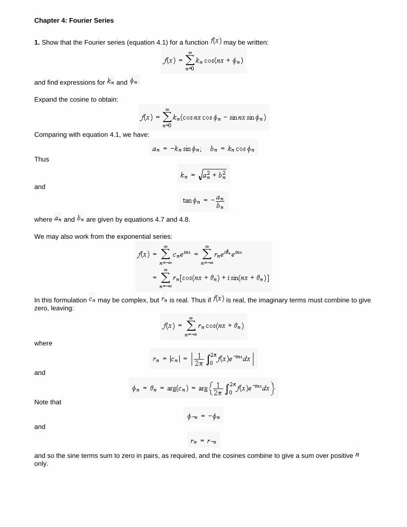
Chapter 4: Fourier Series
1. Show that the Fourier series (equation 4.1) for a function may be written:
and find expressions for and
Expand the cosine to obtain:
Comparing with equation 4.1, we have:
Thus
and
where and are given by equations 4.7 and 4.8.
We may also work from the exponential series:
In this formulation may be complex, but is real. Thus if is real, the imaginary terms must combine to give zero, leaving:
where
and
Note that
and
and so the sine terms sum to zero in pairs, as required, and the cosines combine to give a sum over positive only.
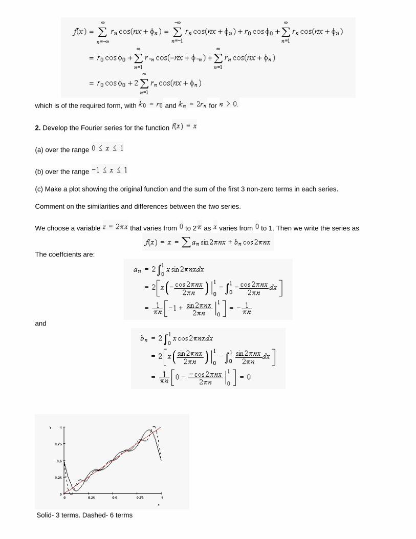
which is of the required form, with and for
2. Develop the Fourier series for the function
(a) over the range
(b) over the range
(c) Make a plot showing the original function and the sum of the first 3 non-zero terms in each series.
Comment on the similarities and differences between the two series.
We choose a variable that varies from to 2 as varies from to 1. Then we write the series as
The coeffcients are:
and
Solid- 3 terms. Dashed- 6 terms
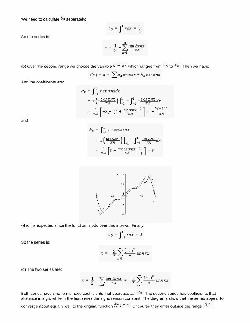
We need to calculate separately:
So the series is:
(b) Over the second range we choose the variable which ranges from to Then we have:
And the coefficents are:
and
which is expected since the function is odd over this interval. Finally:
So the series is:
(c) The two series are:
Both series have sine terms have coefficients that decrease as The second series has coefficients that alternate in sign, while in the first series the signs remain constant. The diagrams show that the series appear to
converge about equally well to the original function Of course they differ outside the range :
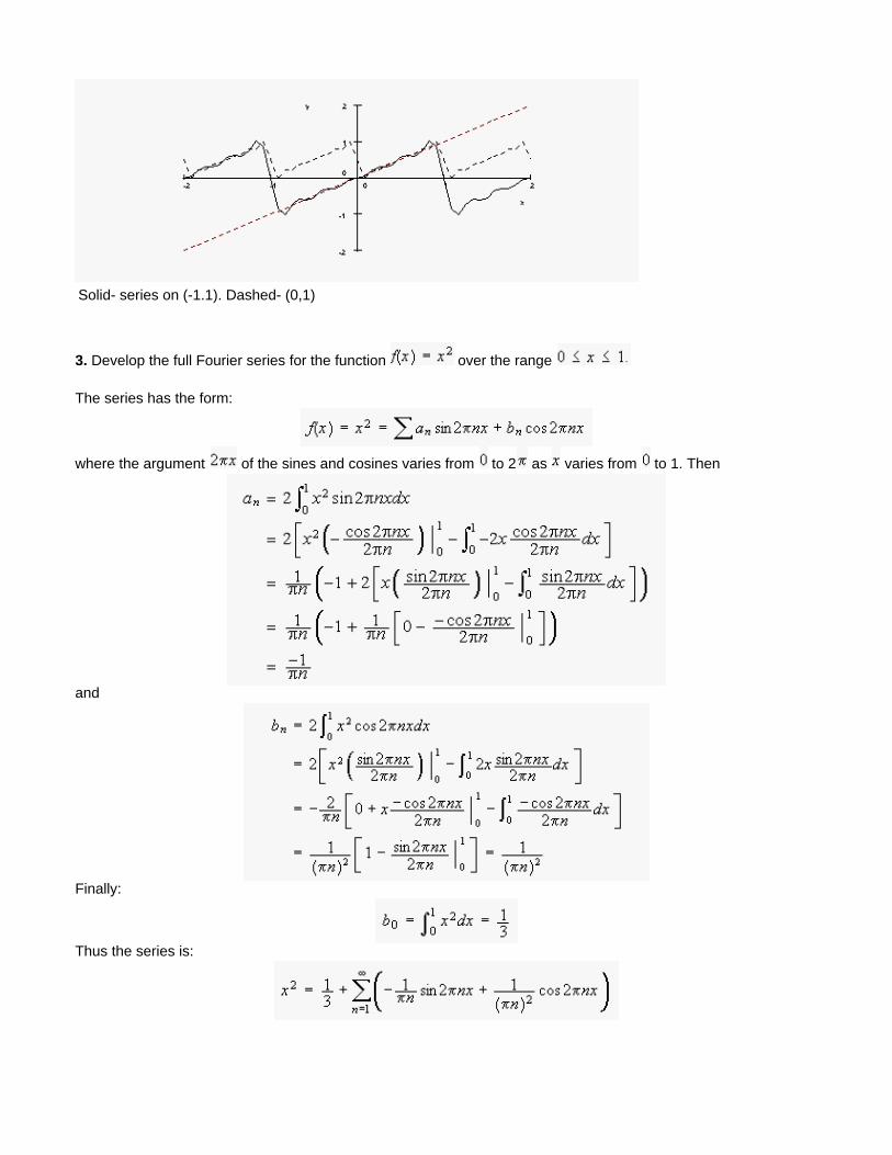
Solid- series on (-1.1). Dashed- (0,1)
3. Develop the full Fourier series for the function over the range
The series has the form:
where the argument of the sines and cosines varies from to 2 as varies from to 1. Then
and
Finally:
Thus the series is:
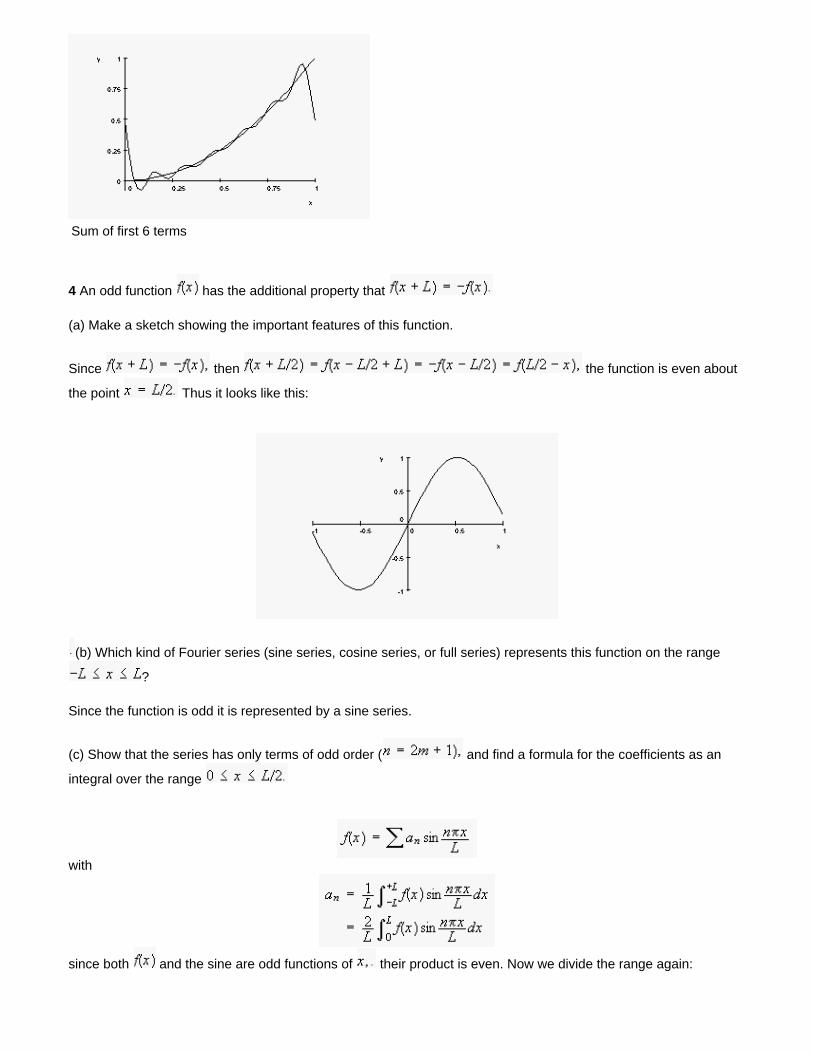
Sum of first 6 terms
4 An odd function has the additional property that
(a) Make a sketch showing the important features of this function.
Since then the function is even about
the point Thus it looks like this:
(b) Which kind of Fourier series (sine series, cosine series, or full series) represents this function on the range
?
Since the function is odd it is represented by a sine series.
(c) Show that the series has only terms of odd order ( and find a formula for the coefficients as an
integral over the range
with
since both and the sine are odd functions of their product is even. Now we divide the range again:
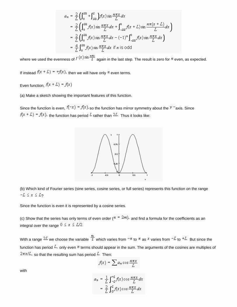
where we used the evenness of again in the last step. The result is zero for even, as expected.
If instead then we will have only even terms.
Even function,
(a) Make a sketch showing the important features of this function.
Since the function is even, so the function has mirror symmetry about the axis. Since
the function has period rather than Thus it looks like:
(b) Which kind of Fourier series (sine series, cosine series, or full series) represents this function on the range
?
Since the function is even it is represented by a cosine series.
(c) Show that the series has only terms of even order ( and find a formula for the coefficients as an
integral over the range
With a range we choose the variable which varies from to as varies from to But since the
function has period only even terms should appear in the sum. The arguments of the cosines are multiples of
so that the resulting sum has period Then:
with
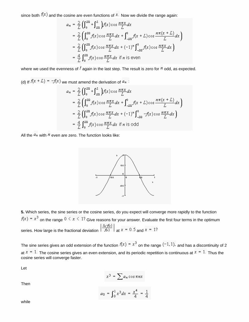
since both and the cosine are even functions of Now we divide the range again:
where we used the evenness of again in the last step. The result is zero for odd, as expected.
(d) If we must amend the derivation of
All the with even are zero. The function looks like:
5. Which series, the sine series or the cosine series, do you expect will converge more rapidly to the function
on the range Give reasons for your answer. Evaluate the first four terms in the optimum
series. How large is the fractional deviation at and
The sine series gives an odd extension of the function on the range and has a discontinuity of 2
at The cosine series gives an even extension, and its periodic repetition is continuous at Thus the cosine series will converge faster.
Let
Then
while
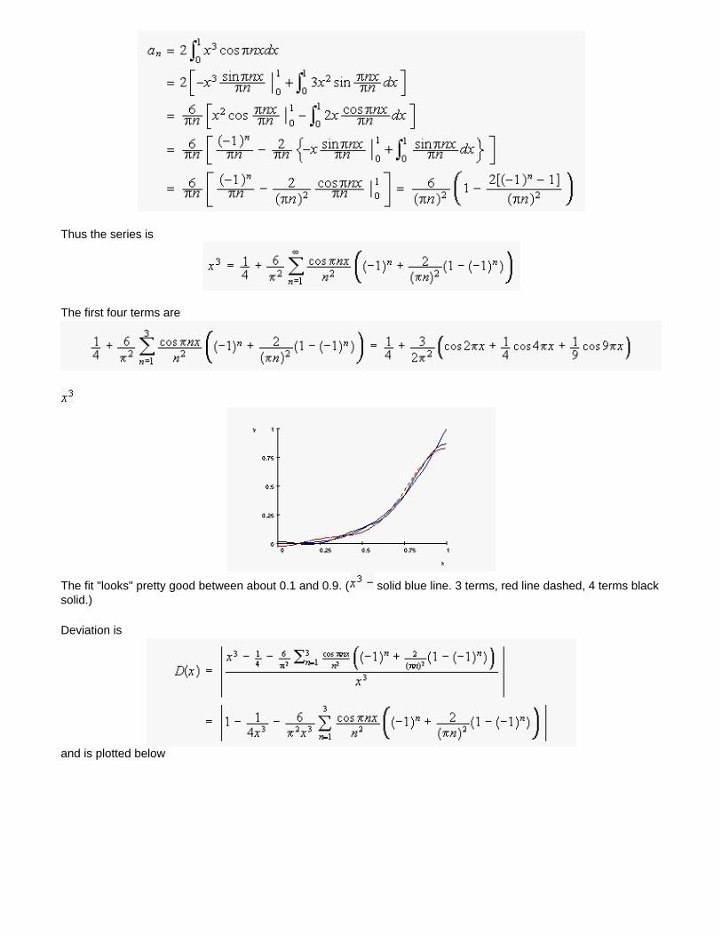
Thus the series is
The first four terms are
The fit "looks" pretty good between about 0.1 and 0.9. ( solid blue line. 3 terms, red line dashed, 4 terms black solid.)
Deviation is
and is plotted below
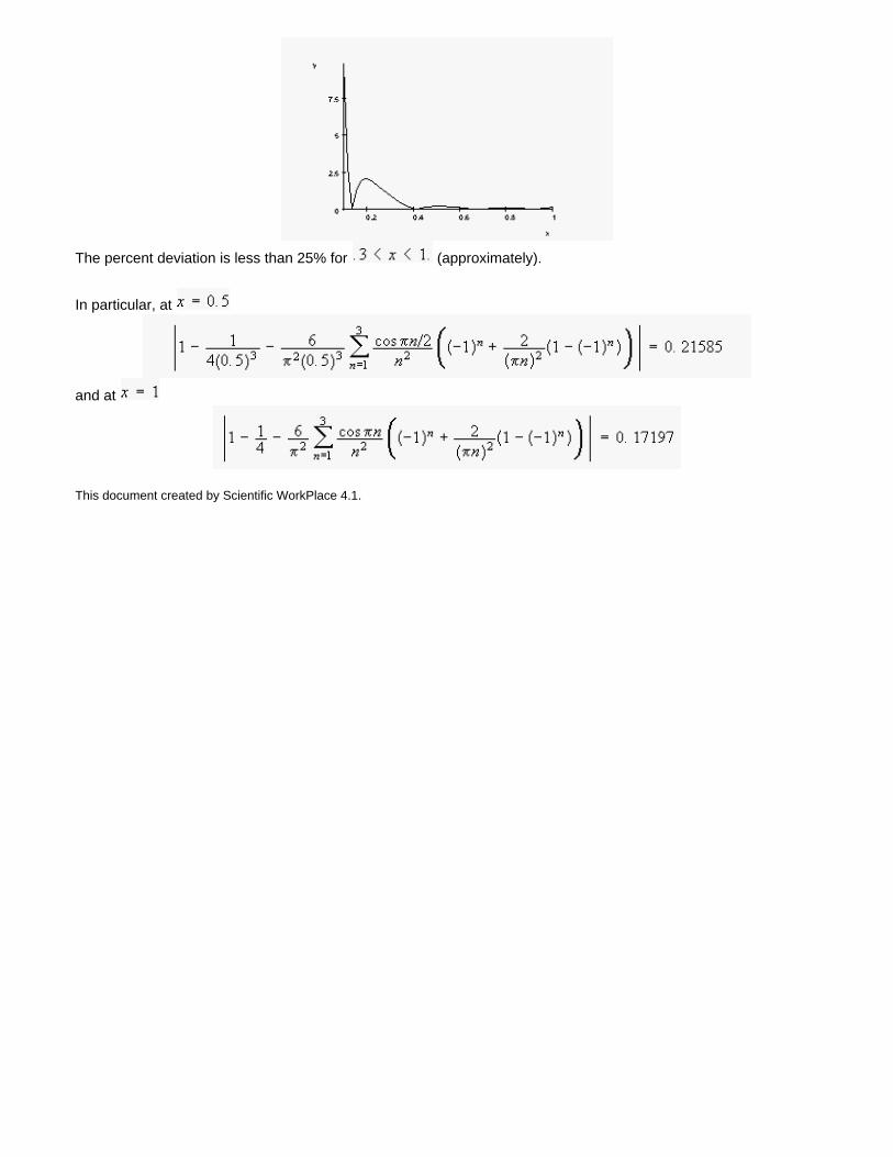
The percent deviation is less than 25% for (approximately).
In particular, at
and at
This document created by Scientific WorkPlace 4.1.
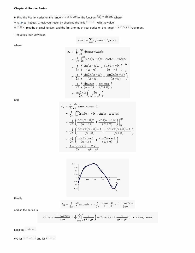
Chapter 4: Fourier Series
6. Find the Fourier series on the range for the function where
is not an integer. Check your result by checking the limit With the value
plot the original function and the first 3 terms of your series on the range Comment.
The series may be written:
where
and
Finally
and so the series is:
Limit as
We let and let
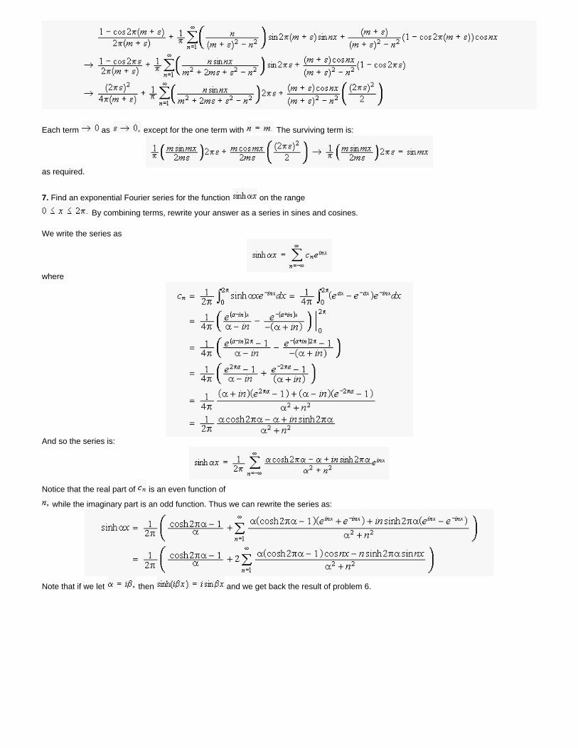
Each term as except for the one term with The surviving term is:
as required.
7. Find an exponential Fourier series for the function on the range
By combining terms, rewrite your answer as a series in sines and cosines.
We write the series as
where
And so the series is:
Notice that the real part of is an even function of
while the imaginary part is an odd function. Thus we can rewrite the series as:
Note that if we let then and we get back the result of problem 6.
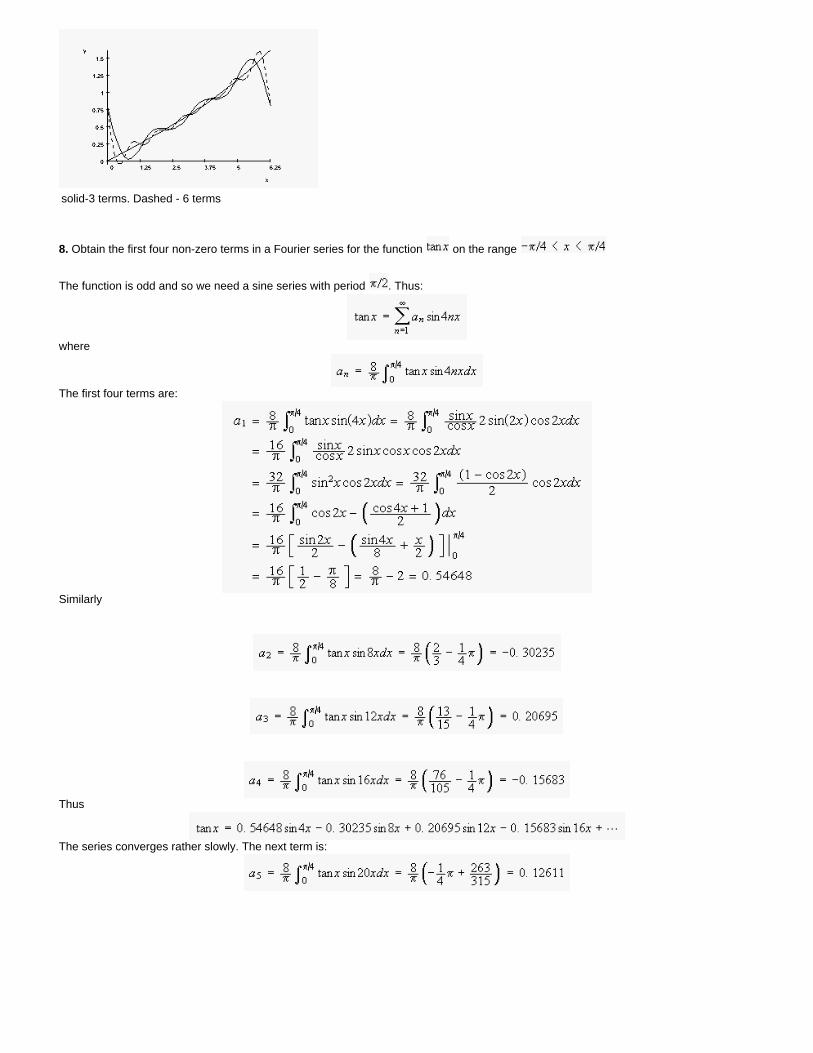
solid-3 terms. Dashed - 6 terms
8. Obtain the first four non-zero terms in a Fourier series for the function on the range
The function is odd and so we need a sine series with period . Thus:
where
The first four terms are:
Similarly
Thus
The series converges rather slowly. The next term is:
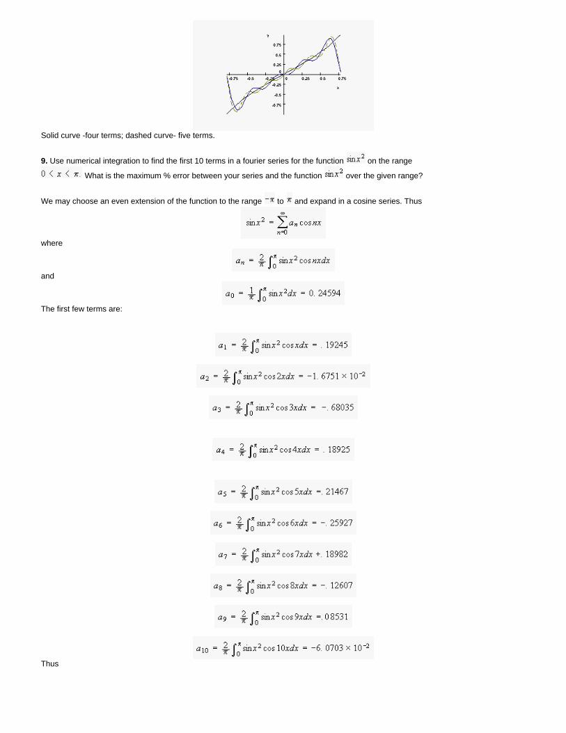
Solid curve -four terms; dashed curve- five terms.
9. Use numerical integration to find the first 10 terms in a fourier series for the function on the range
What is the maximum % error between your series and the function over the given range?
We may choose an even extension of the function to the range to and expand in a cosine series. Thus
where
and
The first few terms are:
Thus
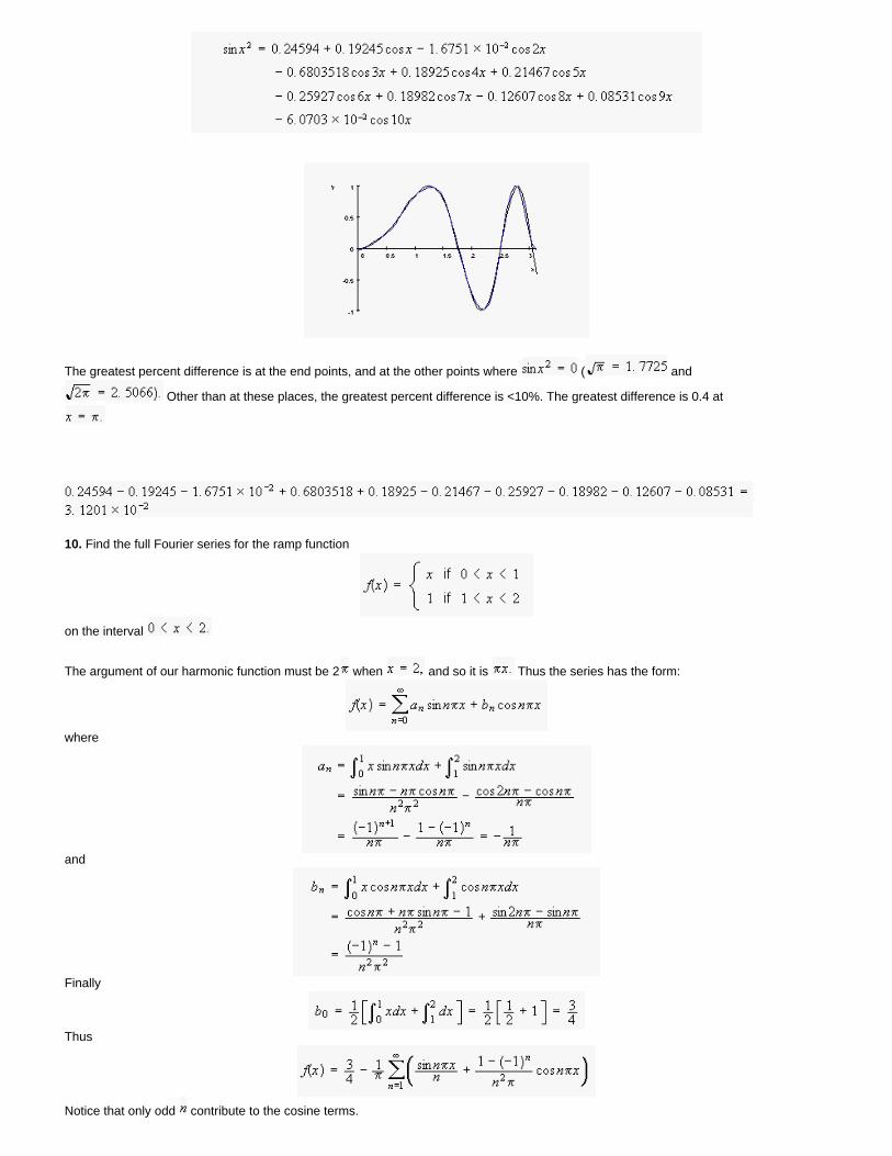
The greatest percent difference is at the end points, and at the other points where ( and
Other than at these places, the greatest percent difference is <10%. The greatest difference is 0.4 at
10. Find the full Fourier series for the ramp function
on the interval
The argument of our harmonic function must be 2 when and so it is Thus the series has the form:
where
and
Finally
Thus
Notice that only odd contribute to the cosine terms.
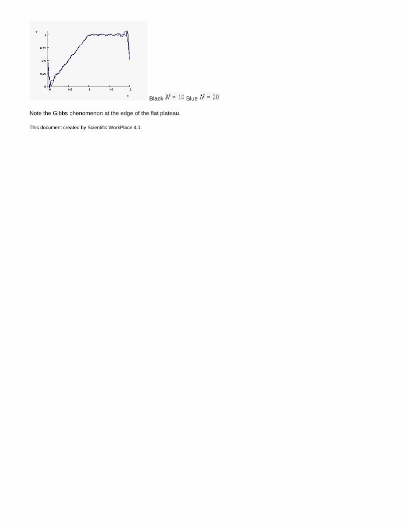
Black Blue
Note the Gibbs phenomenon at the edge of the flat plateau.
This document created by Scientific WorkPlace 4.1.
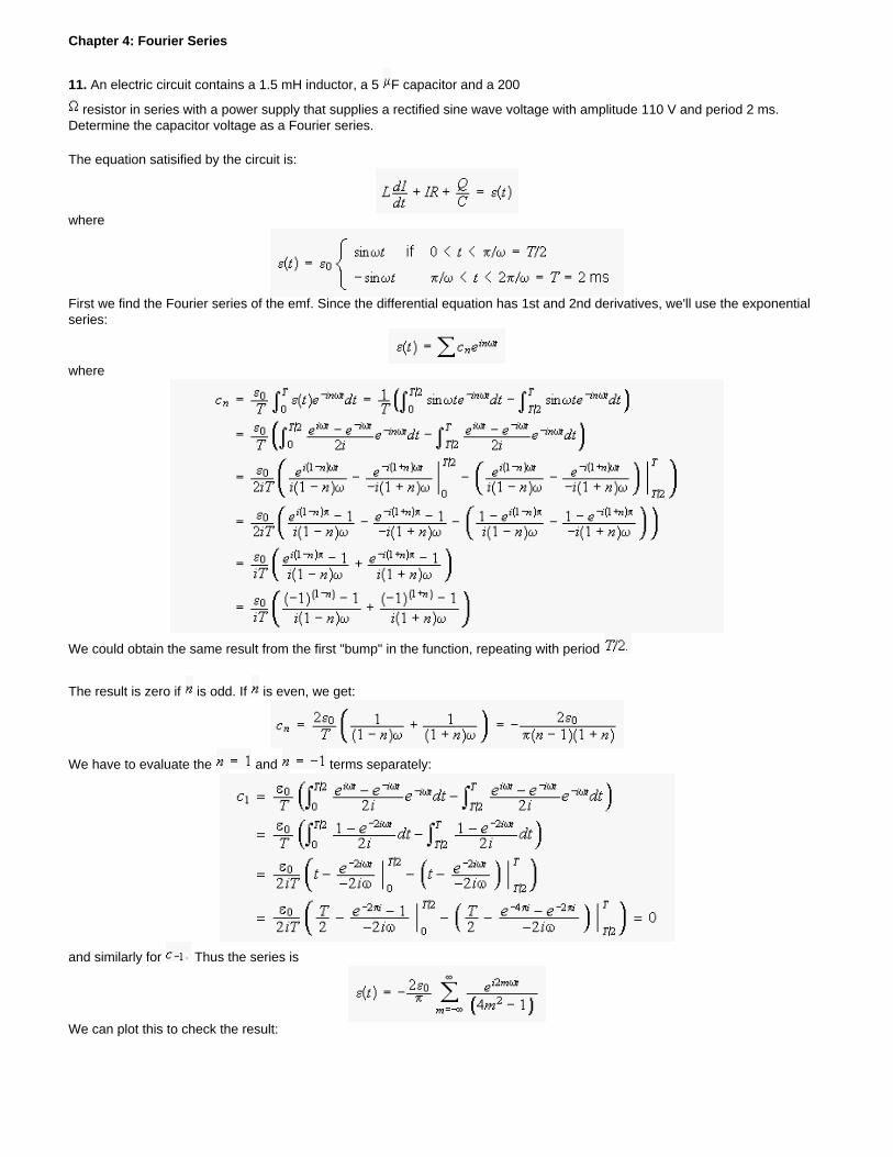
Chapter 4: Fourier Series
11. An electric circuit contains a 1.5 mH inductor, a 5 F capacitor and a 200
resistor in series with a power supply that supplies a rectified sine wave voltage with amplitude 110 V and period 2 ms. Determine the capacitor voltage as a Fourier series.
The equation satisified by the circuit is:
where
First we find the Fourier series of the emf. Since the differential equation has 1st and 2nd derivatives, we'll use the exponential series:
where
We could obtain the same result from the first "bump" in the function, repeating with period
The result is zero if is odd. If is even, we get:
We have to evaluate the and terms separately:
and similarly for Thus the series is
We can plot this to check the result:
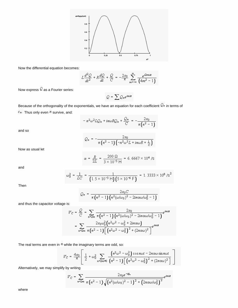
Now the differential equation becomes:
Now express as a Fourier series:
Because of the orthogonality of the exponentials, we have an equation for each coefficient in terms of
Thus only even survive, and:
and so
Now as usual let
and
Then
and thus the capacitor voltage is:
The real terms are even in while the imaginary terms are odd, so:
Alternatively, we may simplify by writing
where

Both expressions give the real result:
The Fourier component may be large for any close to Now
so
and so could be large if is small. However, it is not:
so
and
The first few terms are:
where
Notice we want an angle whose sine is negative and cosine is also negative, so the correct quadrant is the third:
Here we want a negative sine but positive cosine. Thus
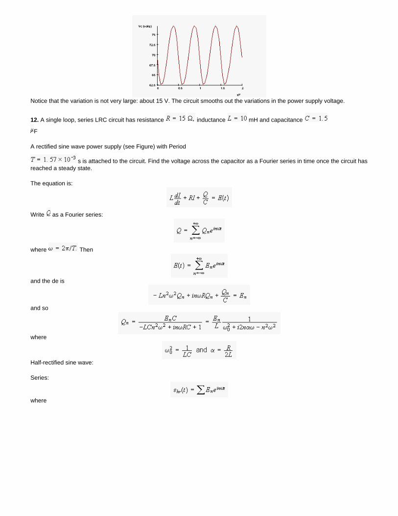
Notice that the variation is not very large: about 15 V. The circuit smooths out the variations in the power supply voltage.
12. A single loop, series LRC circuit has resistance inductance mH and capacitance
F
A rectified sine wave power supply (see Figure) with Period
s is attached to the circuit. Find the voltage across the capacitor as a Fourier series in time once the circuit has reached a steady state.
The equation is:
Write as a Fourier series:
where Then
and the de is
and so
where
Half-rectified sine wave:
Series:
where
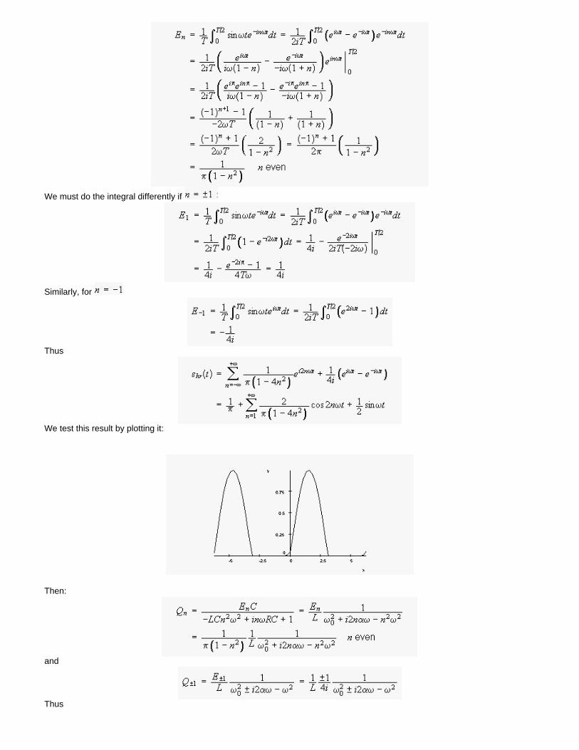
We must do the integral differently if
Similarly, for
Thus
We test this result by plotting it:
Then:
and
Thus
Now we put in the numbers:
and
and
So
and
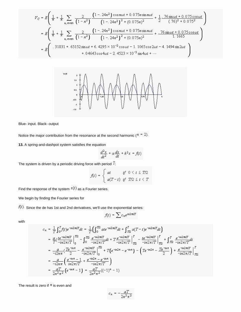
Blue- input. Black- output
Notice the major contribution from the resonance at the second harmonic (
13. A spring-and-dashpot system satisfies the equation
The system is driven by a periodic driving force with period :
Find the response of the system as a Fourier series.
We begin by finding the Fourier series for
Since the de has 1st and 2nd derivatives, we'll use the exponential series:
with
The result is zero if is even and
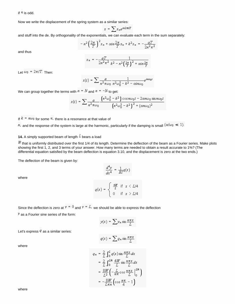
if is odd.
Now we write the displacement of the spring system as a similar series:
and stuff into the de. By orthogonality of the exponentials, we can evaluate each term in the sum separately:
and thus
Let Then:
We can group together the terms with and to get:
If for some there is a resonance at that value of
and the response of the system is large at the harmonic, particularly if the damping is small
14. A simply supported beam of length bears a load
that is uniformly distributed over the first 1/4 of its length. Determine the deflection of the beam as a Fourier series. Make plots showing the first 1, 2, and 3 terms of your answer. How many terms are needed to obtain a result accurate to 1%? (The differential equation satisfied by the beam deflection is equation 3.10, and the displacement is zero at the two ends.)
The deflection of the beam is given by:
where
Since the deflection is zero at and we should be able to express the deflection
as a Fourier sine series of the form:
Let's express as a similar series:
where
where
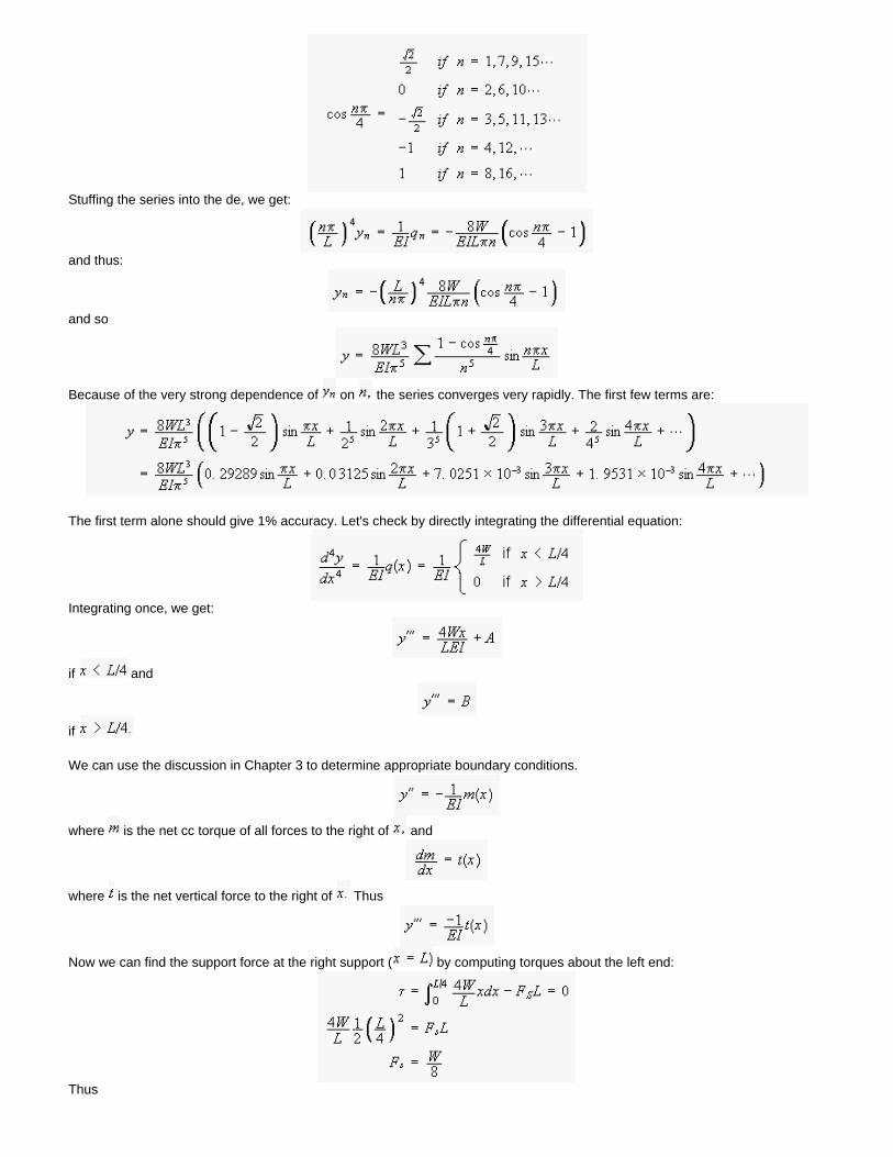
Stuffing the series into the de, we get:
and thus:
and so
Because of the very strong dependence of on the series converges very rapidly. The first few terms are:
The first term alone should give 1% accuracy. Let's check by directly integrating the differential equation:
Integrating once, we get:
if and
if
We can use the discussion in Chapter 3 to determine appropriate boundary conditions.
where is the net cc torque of all forces to the right of and
where is the net vertical force to the right of Thus
Now we can find the support force at the right support ( by computing torques about the left end:
Thus
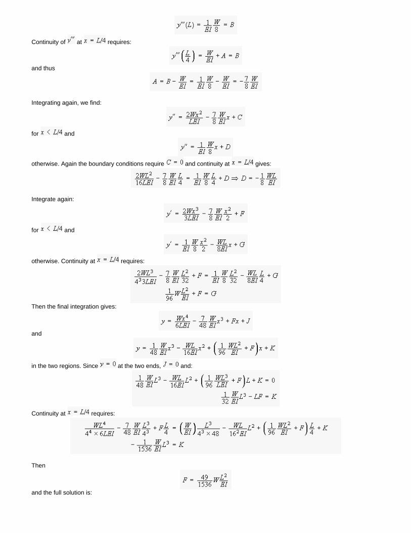
Continuity of at requires:
and thus
Integrating again, we find:
for and
otherwise. Again the boundary conditions require and continuity at gives:
Integrate again:
for and
otherwise. Continuity at requires:
Then the final integration gives:
and
in the two regions. Since at the two ends, and:
Continuity at requires:
Then
and the full solution is:
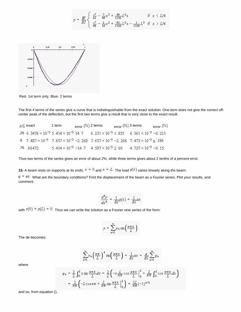
Red- 1st term only. Blue- 2 terms
The first 4 terms of the series give a curve that is indistinguishable from the exact solution. One term does not give the correct off-center peak of the deflection, but the first two terms give a result that is very close to the exact result.
exact 1 term error 2 terms error 3 terms error
.25
.5 0
.75
Thus two terms of the series gives an error of about 2%, while three terms gives about 2 tenths of a percent error.
15. A beam rests on supports at its ends, and The load varies linearly along the beam:
What are the boundary conditions? Find the displacement of the beam as a Fourier series. Plot your results, and comment.
with Thus we can write the solution as a Fourier sine series of the form:
The de becomes:
where
and so, from equation (),
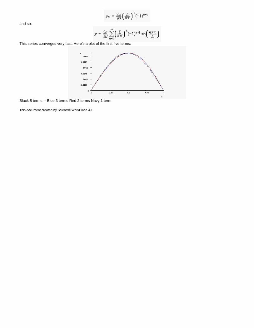
and so:
This series converges very fast. Here's a plot of the first five terms:
Black 5 terms -- Blue 3 terms Red 2 terms Navy 1 term
This document created by Scientific WorkPlace 4.1.
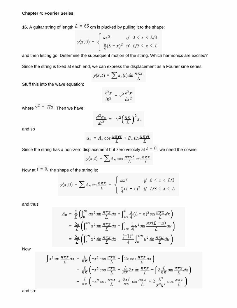
Chapter 4: Fourier Series
16. A guitar string of length cm is plucked by pulling it to the shape:
and then letting go. Determine the subsequent motion of the string. Which harmonics are excited?
Since the string is fixed at each end, we can express the displacement as a Fourier sine series:
Stuff this into the wave equation:
where Then we have:
and so
Since the string has a non-zero displacement but zero velocity at we need the cosine:
Now at the shape of the string is:
and thus
Now
and so:
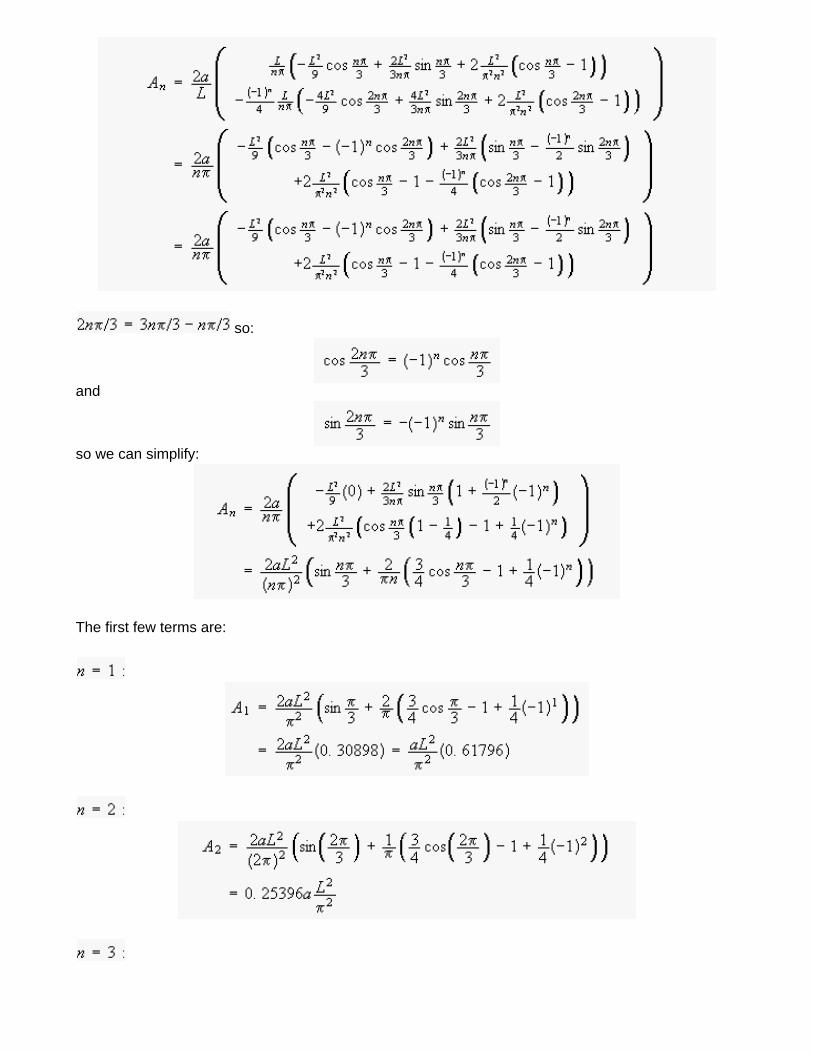
so:
and
so we can simplify:
The first few terms are:
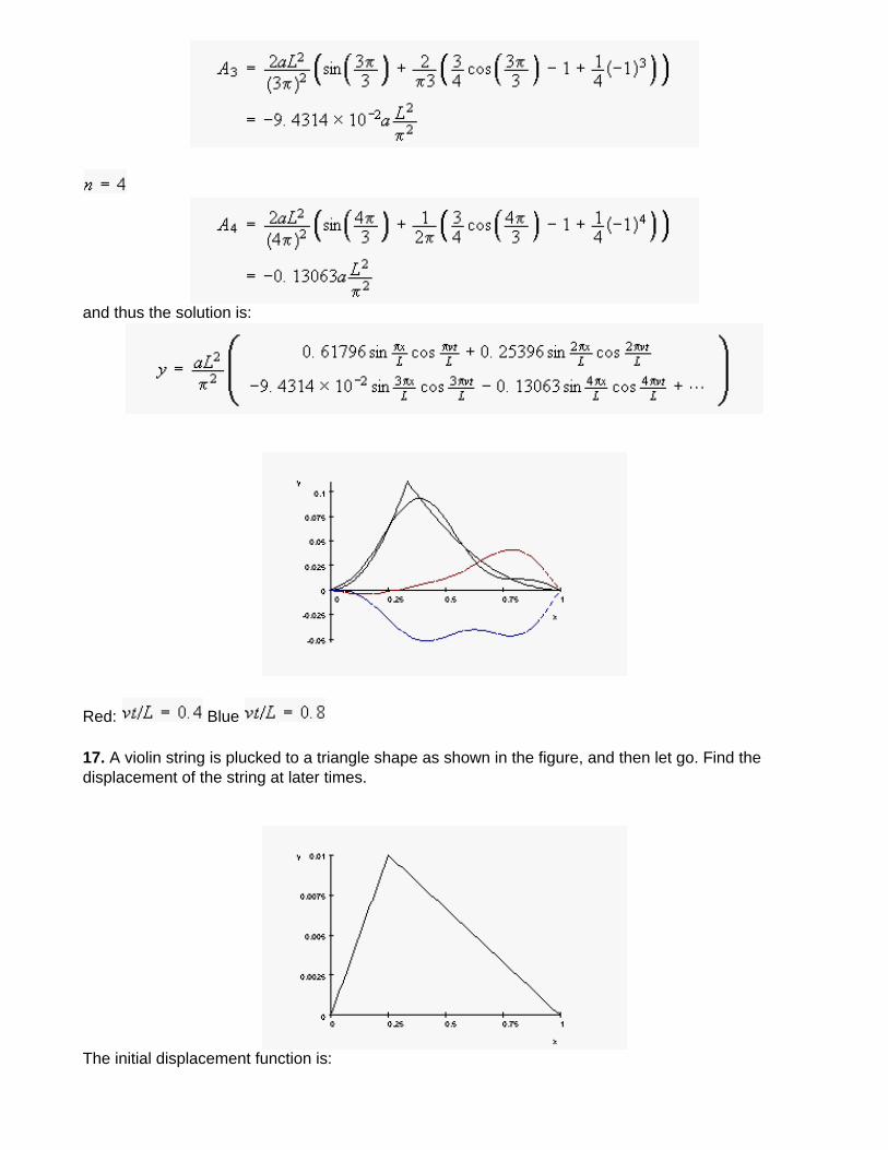
and thus the solution is:
Red: Blue
17. A violin string is plucked to a triangle shape as shown in the figure, and then let go. Find the displacement of the string at later times.
The initial displacement function is:
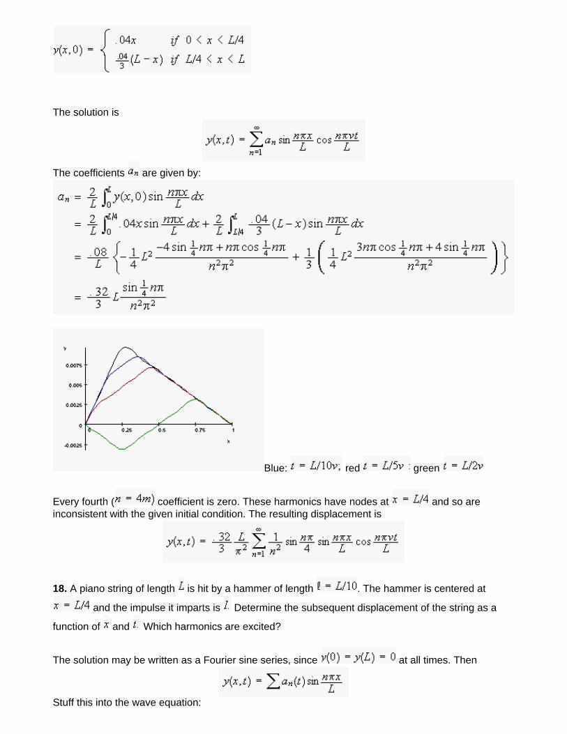
The solution is
The coefficients are given by:
Blue: red green
Every fourth ( coefficient is zero. These harmonics have nodes at and so are inconsistent with the given initial condition. The resulting displacement is
18. A piano string of length is hit by a hammer of length . The hammer is centered at
and the impulse it imparts is Determine the subsequent displacement of the string as a
function of and Which harmonics are excited?
The solution may be written as a Fourier sine series, since at all times. Then
Stuff this into the wave equation:
where Then we have:
and so
Now since the string displacement is zero at we need the sine function. Thus:
Immediately after the hammer hits, the string velocity is not zero. Using the impulse momentum theorem:
Thus
The left hand side is:
Thus
Thus:
and the displacement of the string is:
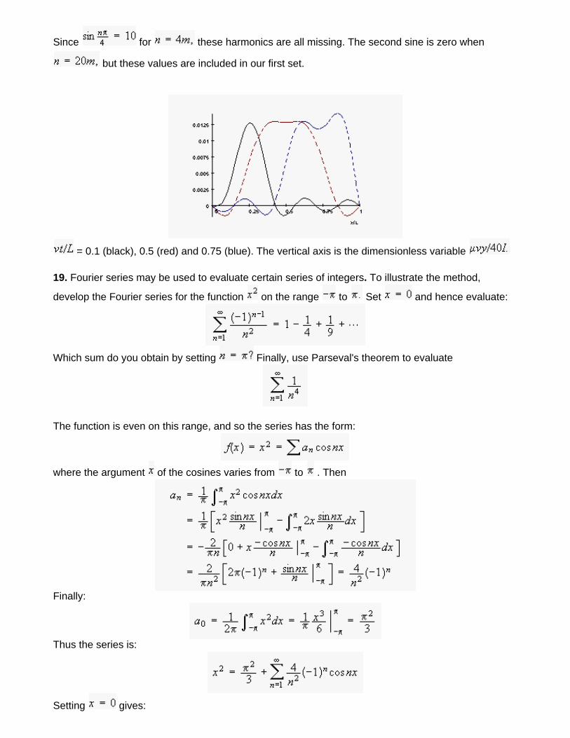
Since for these harmonics are all missing. The second sine is zero when
but these values are included in our first set.
= 0.1 (black), 0.5 (red) and 0.75 (blue). The vertical axis is the dimensionless variable
19. Fourier series may be used to evaluate certain series of integers. To illustrate the method,
develop the Fourier series for the function on the range to Set and hence evaluate:
Which sum do you obtain by setting Finally, use Parseval's theorem to evaluate
The function is even on this range, and so the series has the form:
where the argument of the cosines varies from to . Then
Finally:
Thus the series is:
Setting gives:
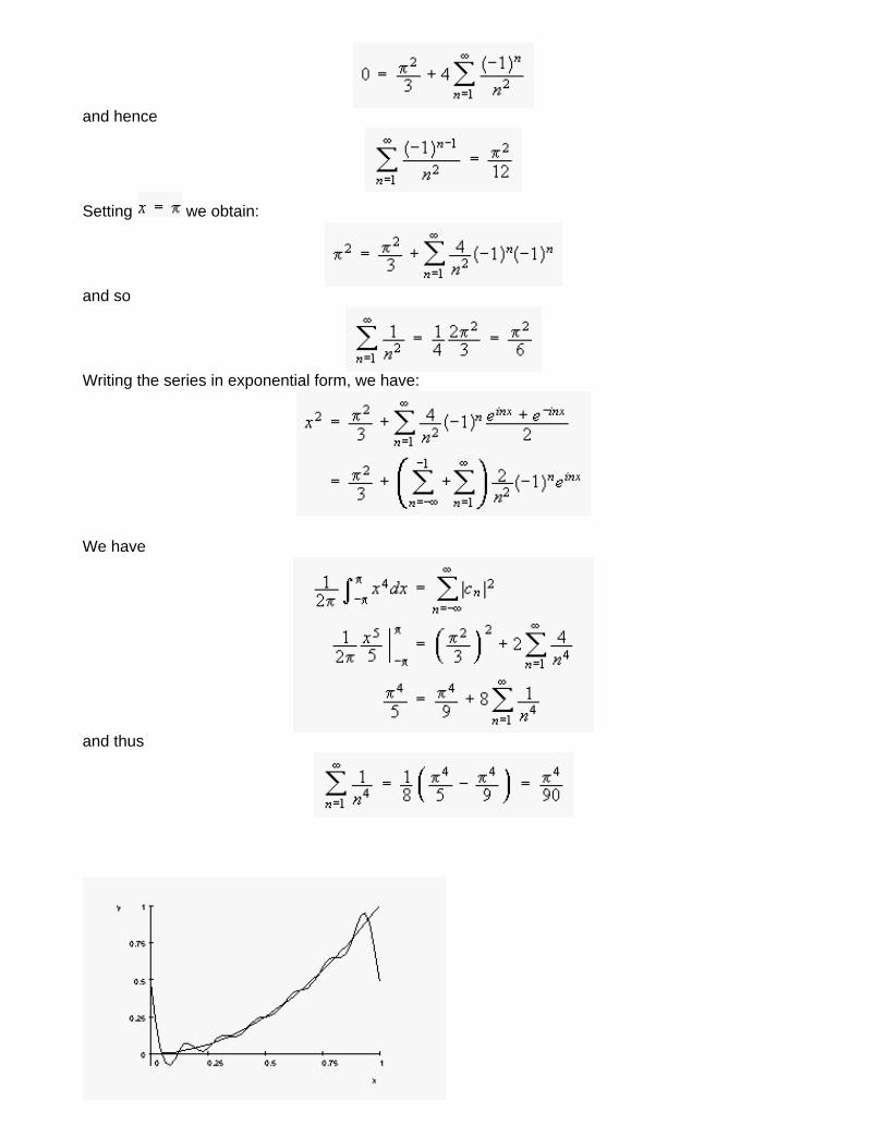
and hence
Setting we obtain:
and so
Writing the series in exponential form, we have:
We have
and thus
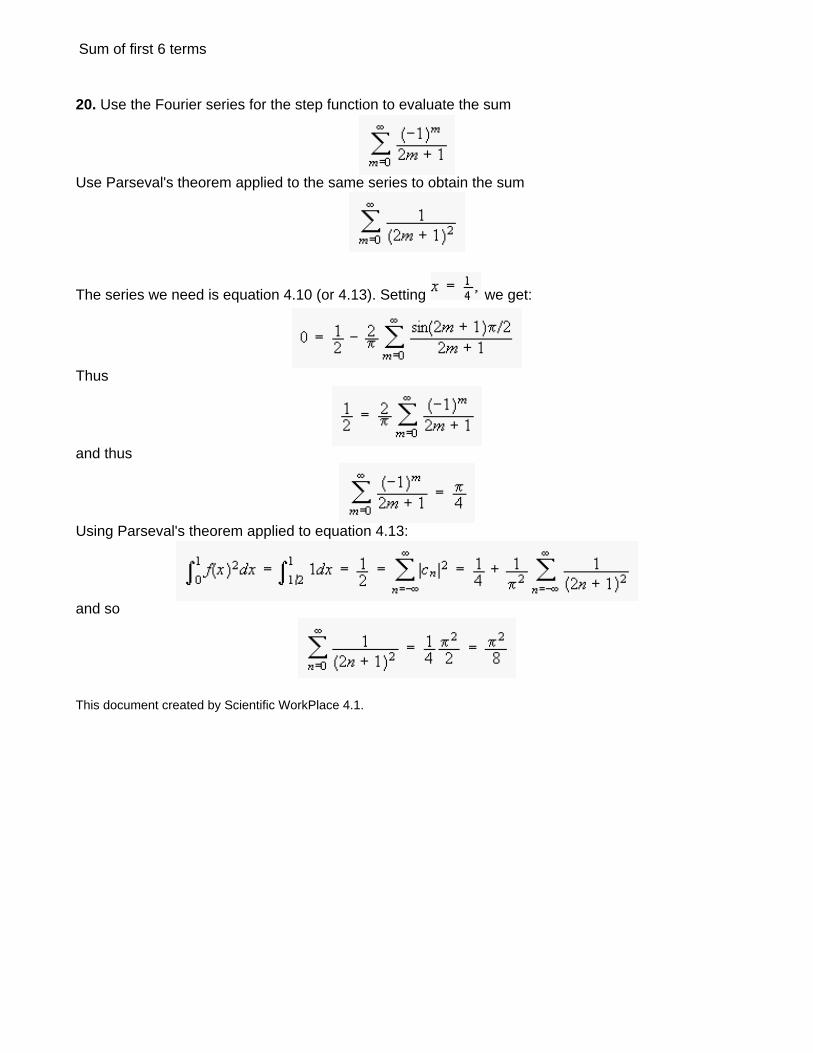
Sum of first 6 terms
20. Use the Fourier series for the step function to evaluate the sum
Use Parseval's theorem applied to the same series to obtain the sum
The series we need is equation 4.10 (or 4.13). Setting we get:
Thus
and thus
Using Parseval's theorem applied to equation 4.13:
and so
This document created by Scientific WorkPlace 4.1.
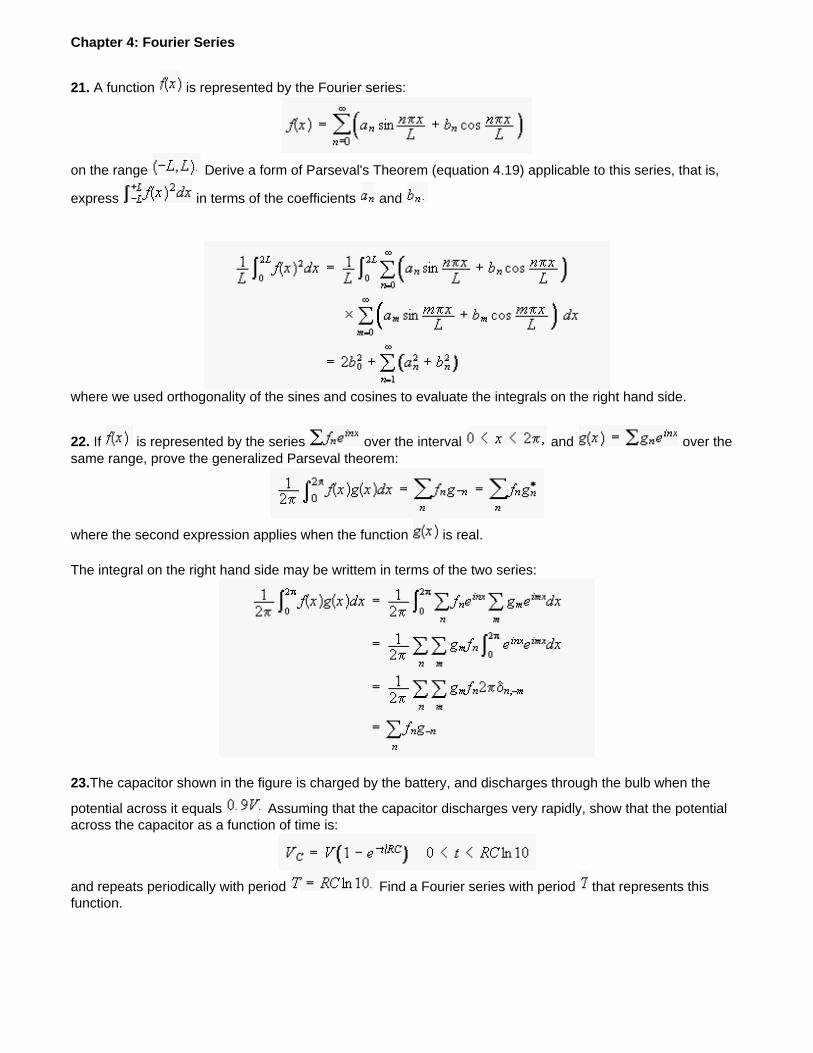
Chapter 4: Fourier Series
21. A function is represented by the Fourier series:
on the range Derive a form of Parseval's Theorem (equation 4.19) applicable to this series, that is,
express in terms of the coefficients and
where we used orthogonality of the sines and cosines to evaluate the integrals on the right hand side.
22. If is represented by the series over the interval and over the same range, prove the generalized Parseval theorem:
where the second expression applies when the function is real.
The integral on the right hand side may be writtem in terms of the two series:
23.The capacitor shown in the figure is charged by the battery, and discharges through the bulb when the
potential across it equals Assuming that the capacitor discharges very rapidly, show that the potential across the capacitor as a function of time is:
and repeats periodically with period Find a Fourier series with period that represents this function.

To find the period we first find when the capacitor voltage reaches 0.9V.
The coefficients are:
When we have
Thus
Now we combine terms to get a real series:
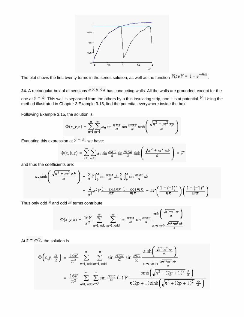
The plot shows the first twenty terms in the series solution, as well as the function .
24. A rectangular box of dimensions has conducting walls. All the walls are grounded, except for the
one at This wall is separated from the others by a thin insulating strip, and it is at potential Using the method illustrated in Chapter 3 Example 3.15, find the potential everywhere inside the box.
Following Example 3.15, the solution is
Evauating this expression at we have:
and thus the coefficients are:
Thus only odd and odd terms contribute
At the solution is
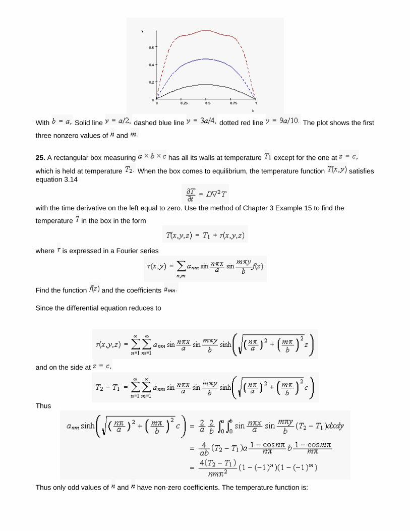
With Solid line dashed blue line dotted red line The plot shows the first
three nonzero values of and
25. A rectangular box measuring has all its walls at temperature except for the one at
which is held at temperature When the box comes to equilibrium, the temperature function satisfies equation 3.14
with the time derivative on the left equal to zero. Use the method of Chapter 3 Example 15 to find the
temperature in the box in the form
where is expressed in a Fourier series
Find the function and the coefficients
Since the differential equation reduces to
and on the side at
Thus
Thus only odd values of and have non-zero coefficients. The temperature function is:
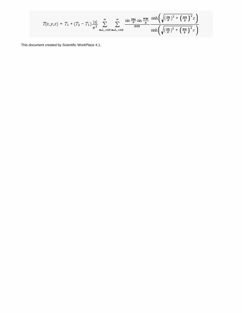
This document created by Scientific WorkPlace 4.1.
Chapter 4: Fourier Series
26. A infinitely long, conducting tube with circular cross section of radius is divided into four pieces by insulating strips running along its length. One of the four pieces is at
potential and the other three are grounded. Solve Laplace's equation in two dimensions
using the method of Example 3.15. Evaluate the solution at and show that the result is a Fourier series. Determine the coefficients, and hence find the potential everywhere inside the tube.
The equation is (equation 1.44)
Using separation of variables, let
Thus the solution for We choose this function because it is periodic with period
and thus the potential at is the same as at as it must be, since both values
represent the same physical point. Then the equation for is:
The solution is a power, where
Thus
and the general solution is of the form
We must eliminate the negative powers because the solution is finite at Thus
and at
a Fourier series for
Equivalently, we may write the series in the form:
To find the coefficients we use the given values for
Thus
If is even, we have
If is odd, we have
While for
Thus
Alternatively, using the series in sines and cosines, we have
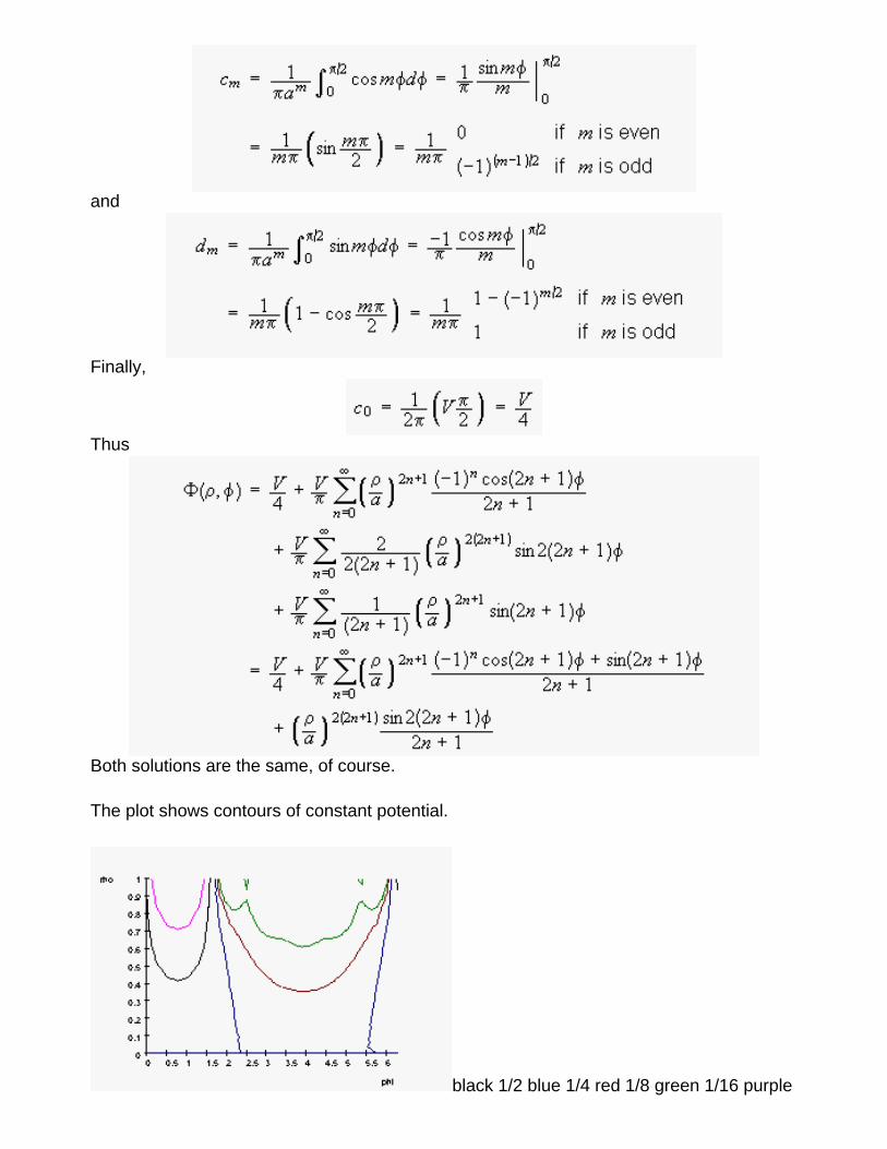
and
Finally,
Thus
Both solutions are the same, of course.
The plot shows contours of constant potential.
black 1/2 blue 1/4 red 1/8 green 1/16 purple
3/4
27. A Fourier series of the form
may be expressed as a power series
where By identifying the power series, the function may be identified. Use this technique to sum the Fourier series
where Check your result by evaluating the Fourier sine series of the function you found.
Let and
For we may sum the series as follows:
Now take the limit from below.
We want to write the argument of the log in the form
where
Thus
and
One solution of this equation is but there are also other possibilities. Since
and we might choose or
If is positive and is also positive. Since
for all has a positive imaginary part and a negative real part, so must
be in the second quadrant, and If then is positive but
is negative, so has a positive imaginary part and a positive real part, so must be in the
first quadrant. Again the appropriate value is
Putting all this together, we get
The function is odd in , since the series is a sine series.
Check by evaluating the Fourier coefficients of our function
as required.
This document created by Scientific WorkPlace 4.1.
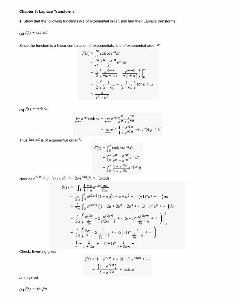
Chapter 5: Laplace Transforms
1. Show that the following functions are of exponential order, and find their Laplace transforms.
(a)
Since the function is a linear combination of exponentials, it is of exponential order
(b)
Thus is of exponential order
Now let Then
Check: Inverting gives
as required.
(c)
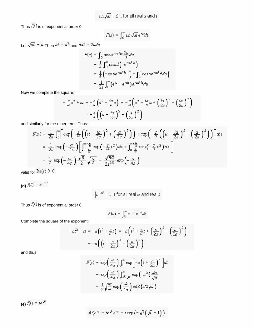
Thus is of exponential order 0.
Let Then and
Now we complete the square:
and similarly for the other term. Thus:
valid for
(d)
Thus is of exponential order 0.
Complete the square of the exponent:
and thus
(e)
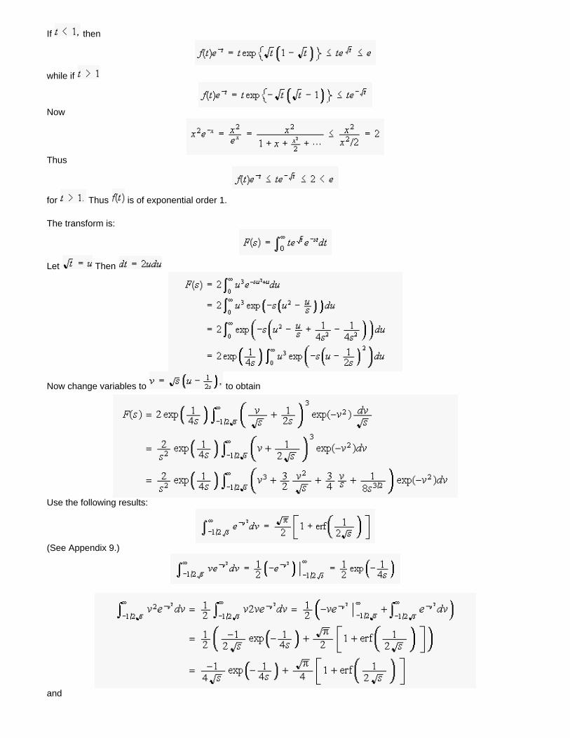
If then
while if
Now
Thus
for Thus is of exponential order 1.
The transform is:
Let Then
Now change variables to to obtain
Use the following results:
(See Appendix 9.)
and
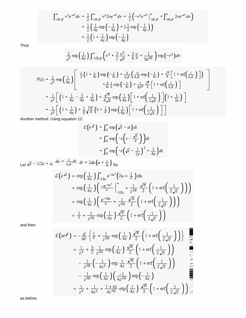
Thus
Another method: Using equation 12:
Let So
and then
as before.
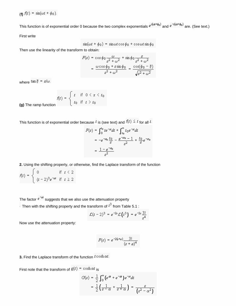
(f)
This function is of exponential order 0 because the two complex exponentials and are. (See text.)
First write
Then use the linearity of the transform to obtain:
where
(g) The ramp function
This function is of exponential order because is (see text) and for all
2. Using the shifting property, or otherwise, find the Laplace transform of the function
The factor suggests that we also use the attenuation property
Then with the shifting property and the transform of from Table 5.1 :
Now use the attenuation property:
3. Find the Laplace transform of the function
First note that the transform of is
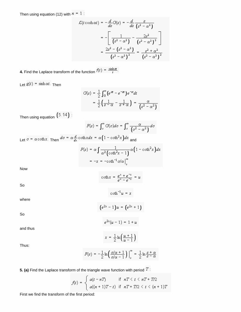
Then using equation (12) with
4. Find the Laplace transform of the function
Let Then
Then using equation
Let Then and
Now
So
where
So
and thus
Thus:
5. (a) Find the Laplace transform of the triangle wave function with period
First we find the transform of the first period:
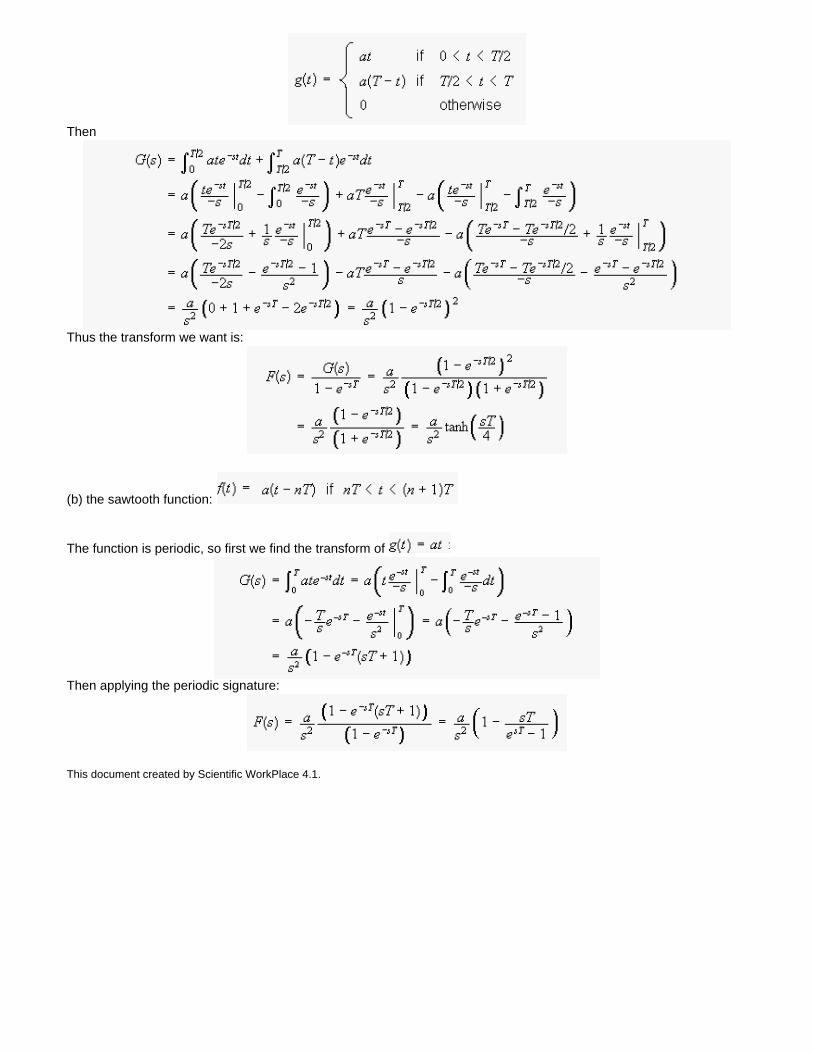
Then
Thus the transform we want is:
(b) the sawtooth function:
The function is periodic, so first we find the transform of
Then applying the periodic signature:
This document created by Scientific WorkPlace 4.1.
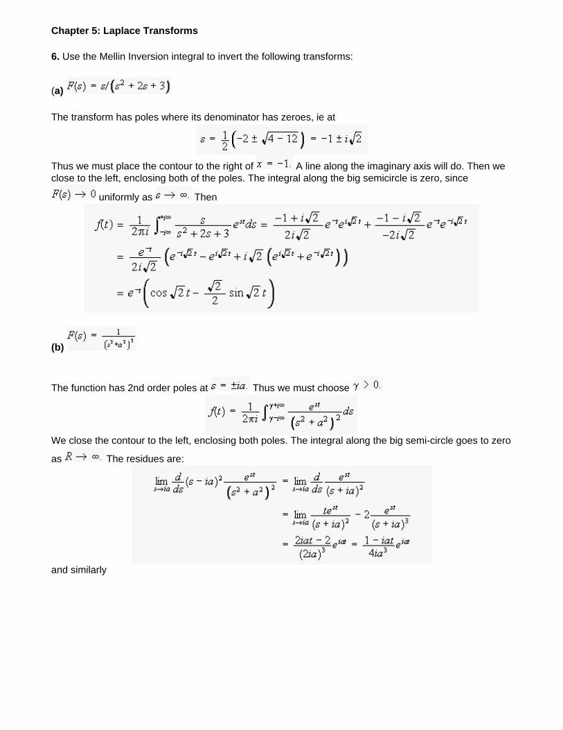
Chapter 5: Laplace Transforms
6. Use the Mellin Inversion integral to invert the following transforms:
(a)
The transform has poles where its denominator has zeroes, ie at
Thus we must place the contour to the right of A line along the imaginary axis will do. Then we close to the left, enclosing both of the poles. The integral along the big semicircle is zero, since
uniformly as Then
(b)
The function has 2nd order poles at Thus we must choose
We close the contour to the left, enclosing both poles. The integral along the big semi-circle goes to zero
as The residues are:
and similarly
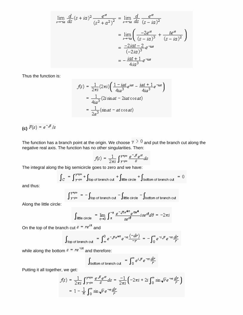
Thus the function is:
(c)
The function has a branch point at the origin. We choose and put the branch cut along the negative real axis. The function has no other singularities. Then:
The integral along the big semicircle goes to zero and we have:
and thus:
Along the little circle:
On the top of the branch cut and
while along the bottom and therefore:
Putting it all together, we get:
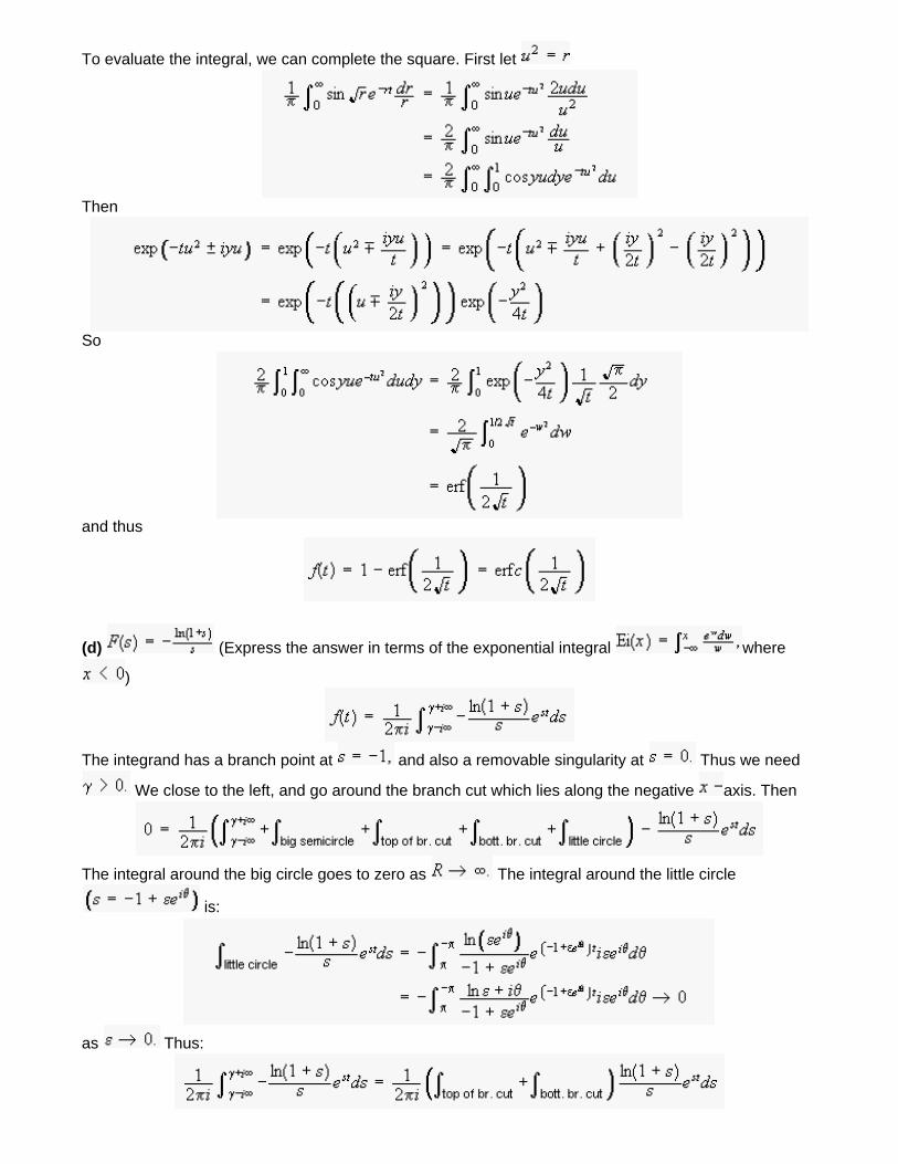
To evaluate the integral, we can complete the square. First let
Then
So
and thus
(d) (Express the answer in terms of the exponential integral where
)
The integrand has a branch point at and also a removable singularity at Thus we need
We close to the left, and go around the branch cut which lies along the negative axis. Then
The integral around the big circle goes to zero as The integral around the little circle
is:
as Thus:
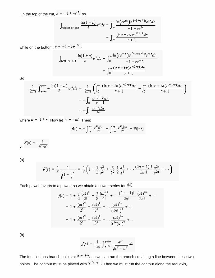
On the top of the cut, so
while on the bottom,
So
where Now let Then:
7.
(a)
Each power inverts to a power, so we obtain a power series for
(b)
The function has branch points at so we can run the branch cut along a line between these two
points. The contour must be placed with Then we must run the contour along the real axis,
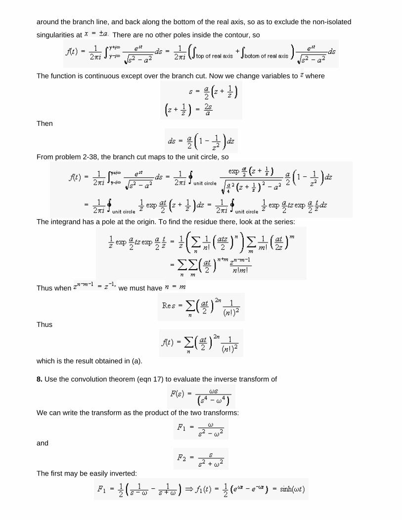
around the branch line, and back along the bottom of the real axis, so as to exclude the non-isolated
singularities at There are no other poles inside the contour, so
The function is continuous except over the branch cut. Now we change variables to where
Then
From problem 2-38, the branch cut maps to the unit circle, so
The integrand has a pole at the origin. To find the residue there, look at the series:
Thus when we must have
Thus
which is the result obtained in (a).
8. Use the convolution theorem (eqn 17) to evaluate the inverse transform of
We can write the transform as the product of the two transforms:
and
The first may be easily inverted:
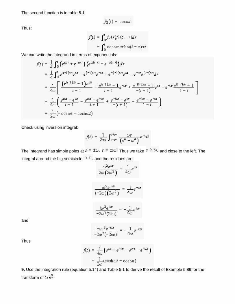
The second function is in table 5.1:
Thus:
We can write the integrand in terms of exponentials:
Check using inversion integral:
The integrand has simple poles at Thus we take and close to the left. The
integral around the big semicircle and the residues are:
and
Thus
9. Use the integration rule (equation 5.14) and Table 5.1 to derive the result of Example 5.89 for the
transform of 1/
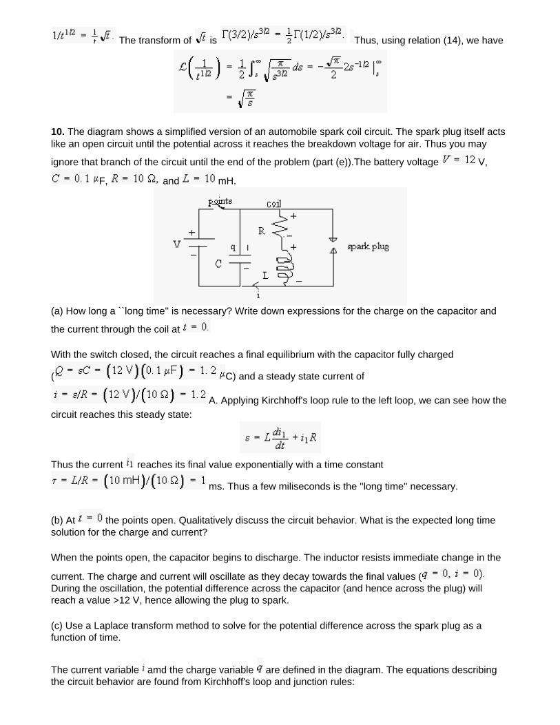
The transform of is Thus, using relation (14), we have
10. The diagram shows a simplified version of an automobile spark coil circuit. The spark plug itself acts like an open circuit until the potential across it reaches the breakdown voltage for air. Thus you may
ignore that branch of the circuit until the end of the problem (part (e)).The battery voltage V,
F, and mH.
(a) How long a ``long time'' is necessary? Write down expressions for the charge on the capacitor and
the current through the coil at
With the switch closed, the circuit reaches a final equilibrium with the capacitor fully charged
( C) and a steady state current of
A. Applying Kirchhoff's loop rule to the left loop, we can see how the circuit reaches this steady state:
Thus the current reaches its final value exponentially with a time constant
ms. Thus a few miliseconds is the ''long time'' necessary.
(b) At the points open. Qualitatively discuss the circuit behavior. What is the expected long time solution for the charge and current?
When the points open, the capacitor begins to discharge. The inductor resists immediate change in the
current. The charge and current will oscillate as they decay towards the final values ( During the oscillation, the potential difference across the capacitor (and hence across the plug) will reach a value >12 V, hence allowing the plug to spark.
(c) Use a Laplace transform method to solve for the potential difference across the spark plug as a function of time.
The current variable amd the charge variable are defined in the diagram. The equations describing the circuit behavior are found from Kirchhoff's loop and junction rules:
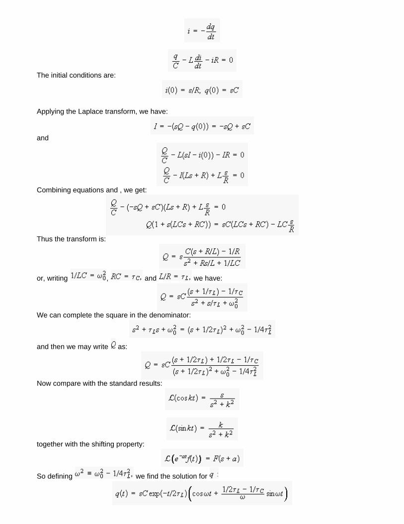
The initial conditions are:
Applying the Laplace transform, we have:
and
Combining equations and , we get:
Thus the transform is:
or, writing , and we have:
We can complete the square in the denominator:
and then we may write as:
Now compare with the standard results:
together with the shifting property:
So defining we find the solution for
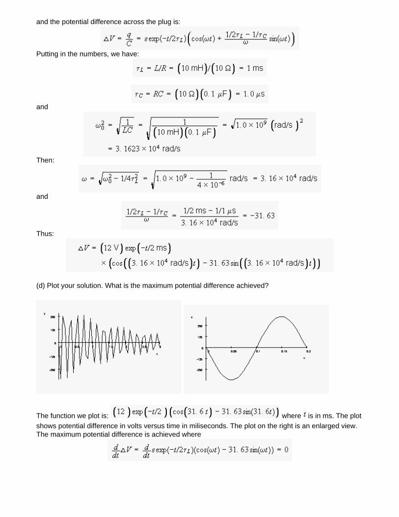
and the potential difference across the plug is:
Putting in the numbers, we have:
and
Then:
and
Thus:
(d) Plot your solution. What is the maximum potential difference achieved?
The function we plot is: where is in ms. The plot shows potential difference in volts versus time in miliseconds. The plot on the right is an enlarged view. The maximum potential difference is achieved where
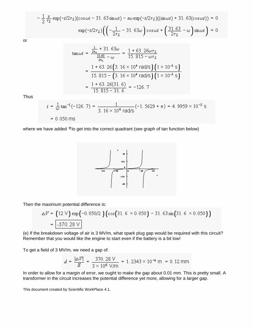
or
Thus
where we have added to get into the correct quadrant (see graph of tan function below)
Then the maximum potential difference is:
(e) If the breakdown voltage of air is 3 MV/m, what spark plug gap would be required with this circuit? Remember that you would like the engine to start even if the battery is a bit low!
To get a field of 3 MV/m, we need a gap of:
In order to allow for a margin of error, we ought to make the gap about 0.01 mm. This is pretty small. A transformer in the circuit increases the potential difference yet more, allowing for a larger gap.
This document created by Scientific WorkPlace 4.1.
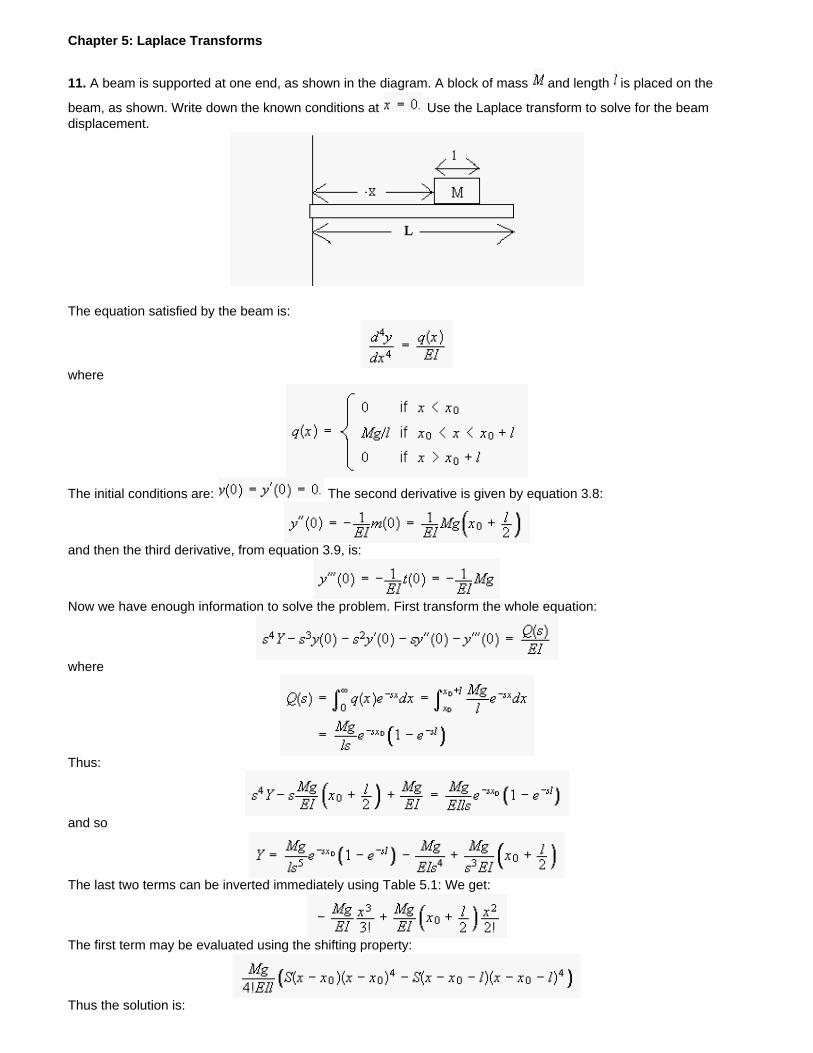
Chapter 5: Laplace Transforms
11. A beam is supported at one end, as shown in the diagram. A block of mass and length is placed on the
beam, as shown. Write down the known conditions at Use the Laplace transform to solve for the beam displacement.
The equation satisfied by the beam is:
where
The initial conditions are: The second derivative is given by equation 3.8:
and then the third derivative, from equation 3.9, is:
Now we have enough information to solve the problem. First transform the whole equation:
where
Thus:
and so
The last two terms can be inverted immediately using Table 5.1: We get:
The first term may be evaluated using the shifting property:
Thus the solution is:
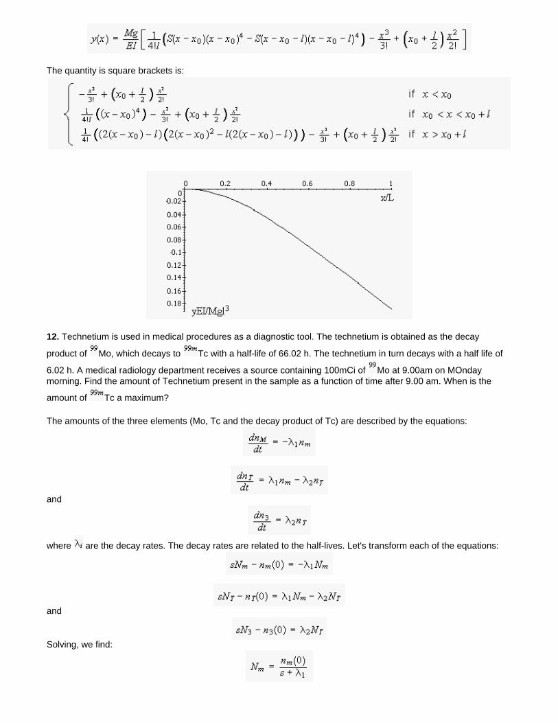
The quantity is square brackets is:
12. Technetium is used in medical procedures as a diagnostic tool. The technetium is obtained as the decay
product of Mo, which decays to Tc with a half-life of 66.02 h. The technetium in turn decays with a half life of
6.02 h. A medical radiology department receives a source containing 100mCi of Mo at 9.00am on MOnday morning. Find the amount of Technetium present in the sample as a function of time after 9.00 am. When is the
amount of Tc a maximum?
The amounts of the three elements (Mo, Tc and the decay product of Tc) are described by the equations:
and
where are the decay rates. The decay rates are related to the half-lives. Let's transform each of the equations:
and
Solving, we find:
and similarly for Inverting the first equation gives:
Thus decreases to one half of its initial value at time where:
and thus
and thus
A similar relation holds for each species. Thus the decay rates are:
and
In the second equation, we set to get:
and inverting, we get:
Thus the maximum amount occurs at time where
or
The maximum Technetium occurs at 9.00 am Monday +22.9 h = h m on Tuesday morning.
13. An overdamped harmonic oscillator satisfies the equation
where and the driving force is a square wave of period Find the displacement if the intial
conditions are Plot the result for and and
First we transform the equation:
and solve for the transform
where
(Example 5.6). Thus:
We can use the shifting property to evaluate each term in the sum, so let's work on the multiplier
The factor tells us that the result is an integral, and we can invert the other factor using the attenuation property. Thus
Thus:
Then with and we get:
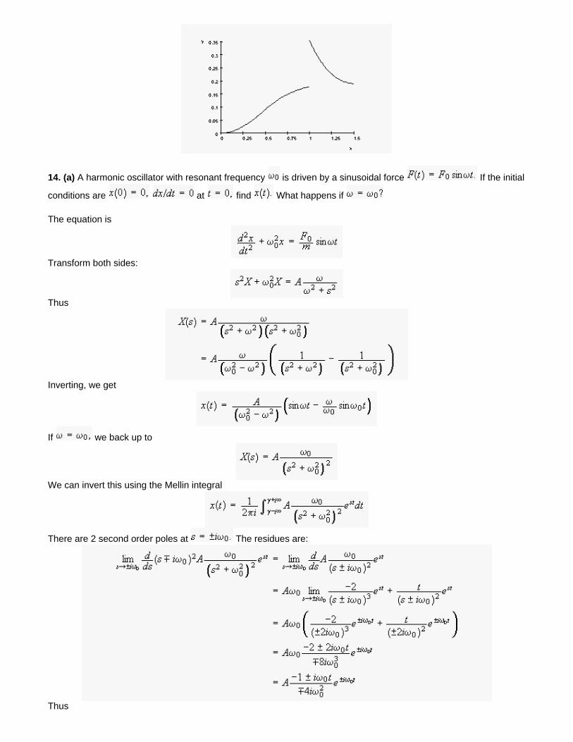
14. (a) A harmonic oscillator with resonant frequency is driven by a sinusoidal force If the initial
conditions are at find What happens if
The equation is
Transform both sides:
Thus
Inverting, we get
If we back up to
We can invert this using the Mellin integral
There are 2 second order poles at The residues are:
Thus
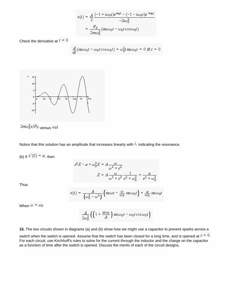
Check the derivative at
versus
Notice that this solution has an amplitude that increases linearly with indicating the resonance.
(b) If then
Thus
When
15. The two circuits shown in diagrams (a) and (b) show how we might use a capacitor to prevent sparks across a
switch when the switch is opened. Assume that the switch has been closed for a long time, and is opened at For each circuit, use Kirchhoff's rules to solve for the current through the inductor and the charge on the capacitor as a function of time after the switch is opened. Discuss the merits of each of the circuit designs.
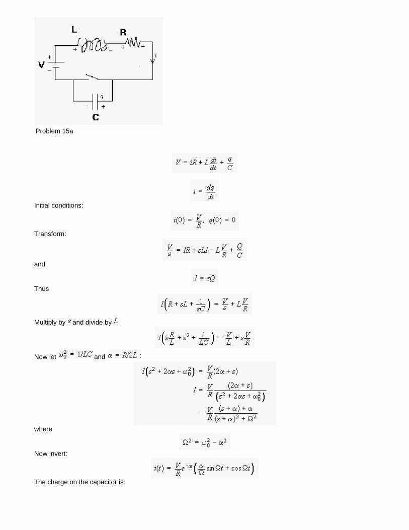
Problem 15a
Initial conditions:
Transform:
and
Thus
Multiply by and divide by
Now let and
where
Now invert:
The charge on the capacitor is:
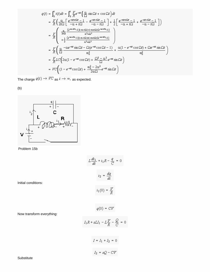
The charge as as expected.
(b)
Problem 15b
Initial conditions:
Now transform everything:
Substitute
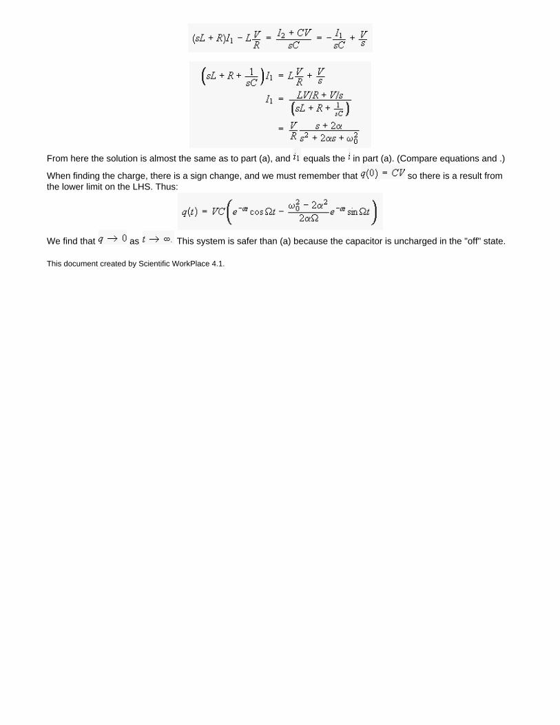
From here the solution is almost the same as to part (a), and equals the in part (a). (Compare equations and .)
When finding the charge, there is a sign change, and we must remember that so there is a result from the lower limit on the LHS. Thus:
We find that as This system is safer than (a) because the capacitor is uncharged in the "off" state.
This document created by Scientific WorkPlace 4.1.
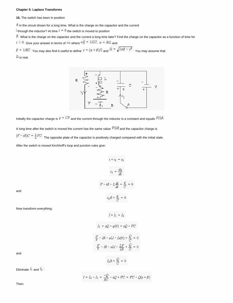
Chapter 5: Laplace Transforms
16. The switch has been in position
in the circuit shown for a long time. What is the charge on the capacitor and the current
through the inductor? At time the switch is moved to position
What is the charge on the capacitor and the current a long time later? Find the charge on the capacitor as a function of time for
Give your answer in terms of where and
You may also find it useful to define and You may assume that
is real.
Initially the capacitor charge is and the current through the inductor is a constant and equals
A long time after the switch is moved the current has the same value and the capacitor charge is
The opposite plate of the capacitor is positively charged compared with the initial state.
After the switch is moved Kirchhoff's loop and junction rules give:
and
Now transform everything:
and
Eliminate and
Then:
So
and
The denominator factors:
We invert using the attenuation property, and the integration rule:
But
So:
Check the limits: At while as as required.
17. The switch has been closed in the circuit shown for a long time, and a constant current flows. What is the charge on the capacitor? At time
the switch is opened. What is the charge on the capacitor and the current through the inductor a long time later? Find the current through
the inductor as a function of time for Give your answer in terms of and where and
.
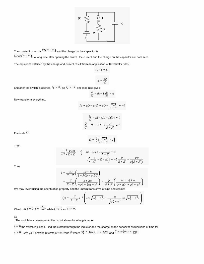
The constant curent is and the charge on the capacitor is
A long time after opening the switch, the current and the charge on the capacitor are both zero.
The equations satsified by the charge and current result from an application of Kirchhoff's rules:
and after the switch is opened, so The loop rule gives:
Now transform everything:
Eliminate
Then
Thus
We may invert using the attentuation property and the known transforms of sine and cosine:
Check: At , while as
18. The switch has been open in the circuit shown for a long time. At
the switch is closed. Find the current through the inductor and the charge on the capacitor as functions of time for
Give your answer in terms of and where , and
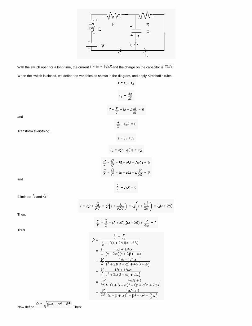
With the switch open for a long time, the current and the charge on the capacitor is
When the switch is closed, we define the variables as shown in the diagram, and apply Kirchhoff's rules:
and
Transform everything:
and
Eliminate and
Then:
Thus
Now define Then:
and inverting gives:
The integral is:
We may simplify the right hand side as follows:
The denominator is:
Thus:
Thus at and as
as required.
Now
We have already done most of the work to invert this. Thus
The current is both at and as again as expected.
19. In the figure shown, capacitor has charge and capacitor is uncharged. At
the switch is closed. The two capacitances are equal. Find the voltage across each capacitor as a function of time for
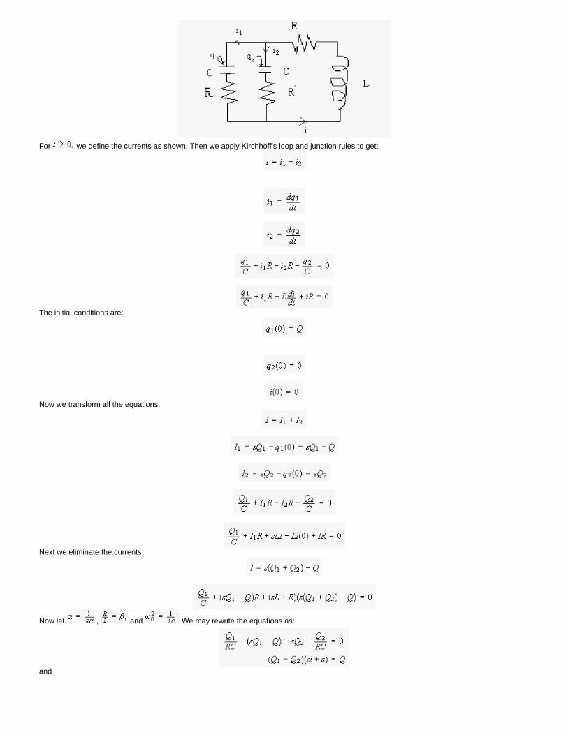
For we define the currents as shown. Then we apply Kirchhoff's loop and junction rules to get:
The initial conditions are:
Now we transform all the equations:
Next we eliminate the currents:
Now let , and We may rewrite the equations as:
and
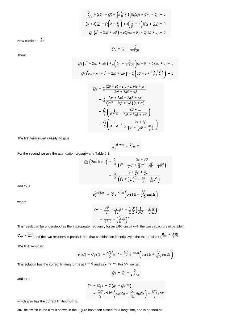
Now eliminate
Then:
The first term inverts easily, to give
For the second we use the attenuation property and Table 5.1:
and thus
where
This result can be understood as the appropriate frequency for an LRC circuit with the two capacitors in parallel (
and the two resistors in parallel, and that combination in series with the third resistor (
The final result is:
This solution has the correct limiting forms at and as For we get:
and thus
which also has the correct limiting forms.
20.The switch in the circuit shown in the Figure has been closed for a long time, and is opened at
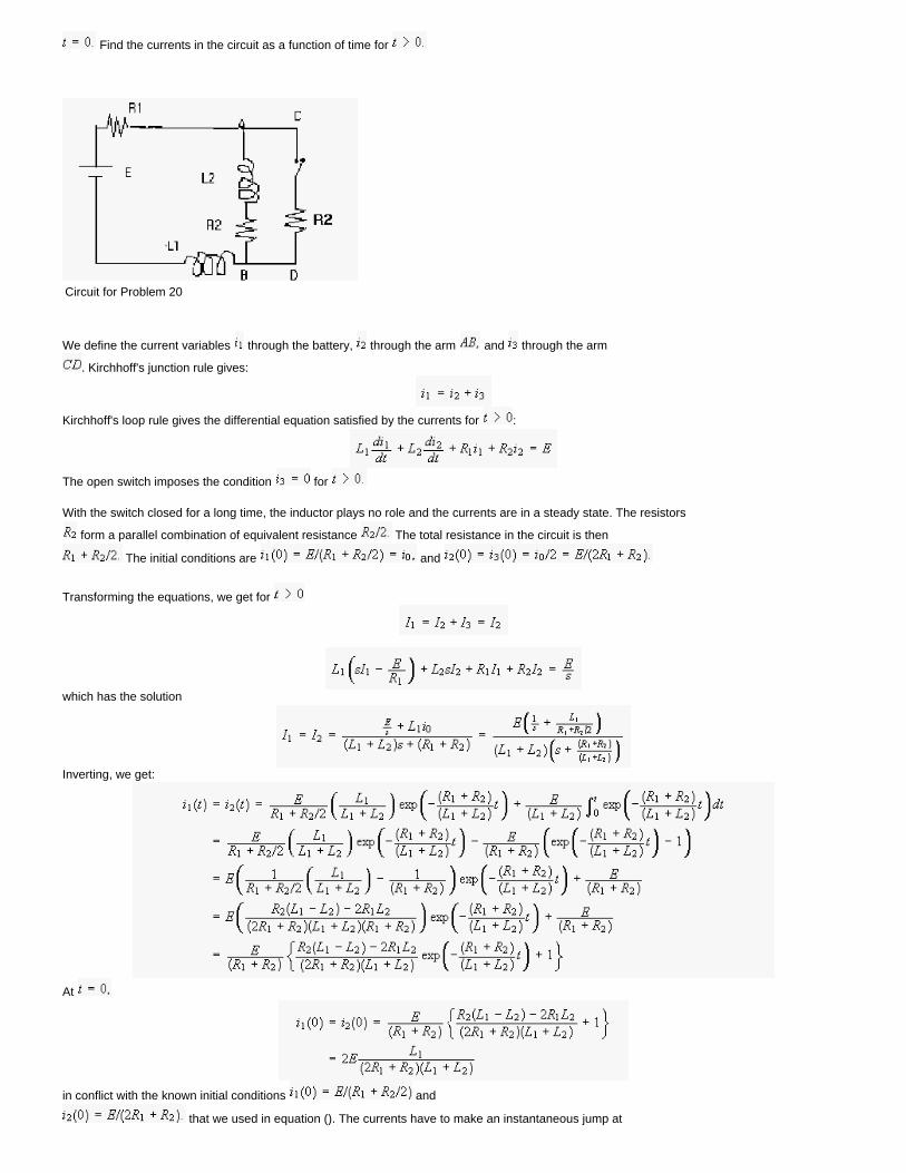
Find the currents in the circuit as a function of time for
Circuit for Problem 20
We define the current variables through the battery, through the arm and through the arm
. Kirchhoff's junction rule gives:
Kirchhoff's loop rule gives the differential equation satisfied by the currents for :
The open switch imposes the condition for
With the switch closed for a long time, the inductor plays no role and the currents are in a steady state. The resistors
form a parallel combination of equivalent resistance The total resistance in the circuit is then
The initial conditions are and
Transforming the equations, we get for
which has the solution
Inverting, we get:
At
in conflict with the known initial conditions and
that we used in equation (). The currents have to make an instantaneous jump at
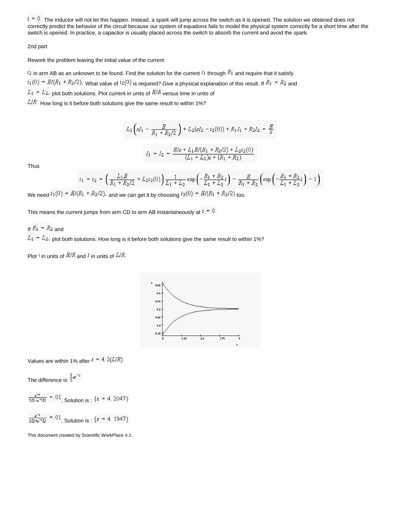
The inductor will not let this happen. Instead, a spark will jump across the switch as it is opened. The solution we obtained does not correctly predict the behavior of the circuit because our system of equations fails to model the physical system correctly for a short time after the switch is opened. In practice, a capacitor is usually placed across the switch to absorb the current and avoid the spark.
2nd part
Rework the problem leaving the initial value of the current
in arm AB as an unknown to be found. Find the solution for the current through and require that it satisfy
What value of is required? Give a physical explanation of this result. If and
plot both solutions. Plot current in units of versus time in units of
How long is it before both solutions give the same result to within 1%?
Thus
We need and we can get it by choosing too.
This means the current jumps from arm CD to arm AB instantaneously at
If and
plot both solutions. How long is it before both solutions give the same result to within 1%?
Plot in units of and in units of
Values are within 1% after
The difference is
, Solution is :
, Solution is :
This document created by Scientific WorkPlace 4.1.
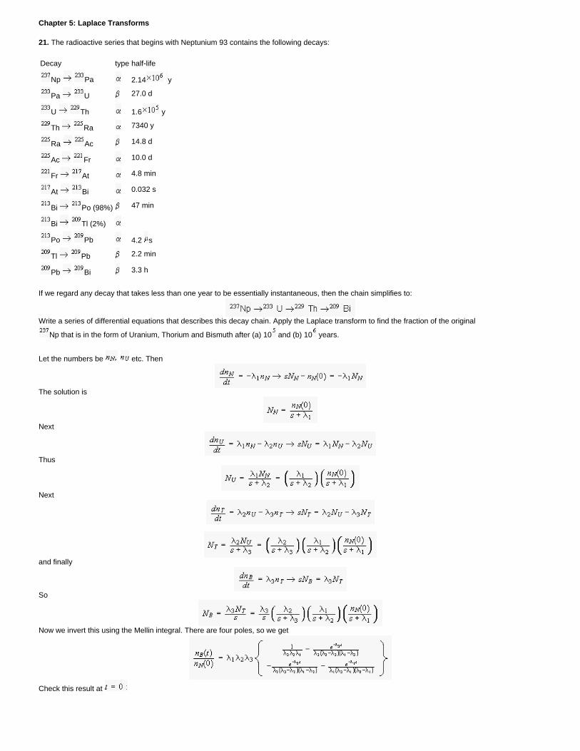
Chapter 5: Laplace Transforms
21. The radioactive series that begins with Neptunium 93 contains the following decays:
Decay type half-life
Np Pa 2.14 y
Pa U 27.0 d
U Th 1.6 y
Th Ra 7340 y
Ra Ac 14.8 d
Ac Fr 10.0 d
Fr At 4.8 min
At Bi 0.032 s
Bi Po (98%) 47 min
Bi Tl (2%)
Po Pb 4.2 s
Tl Pb 2.2 min
Pb Bi 3.3 h
If we regard any decay that takes less than one year to be essentially instantaneous, then the chain simplifies to:
Write a series of differential equations that describes this decay chain. Apply the Laplace transform to find the fraction of the original
Np that is in the form of Uranium, Thorium and Bismuth after (a) 10 and (b) 10 years.
Let the numbers be etc. Then
The solution is
Next
Thus
Next
and finally
So
Now we invert this using the Mellin integral. There are four poles, so we get
Check this result at
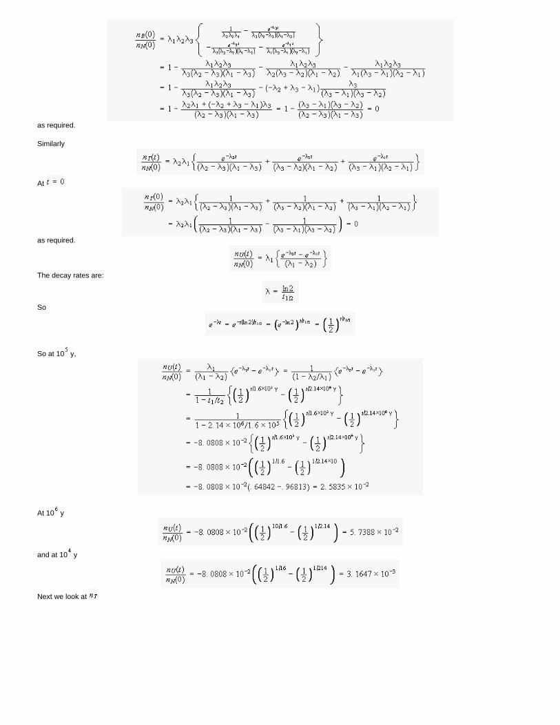
as required.
Similarly
At
as required.
The decay rates are:
So
So at 10 y,
At 10 y
and at 10 y
Next we look at
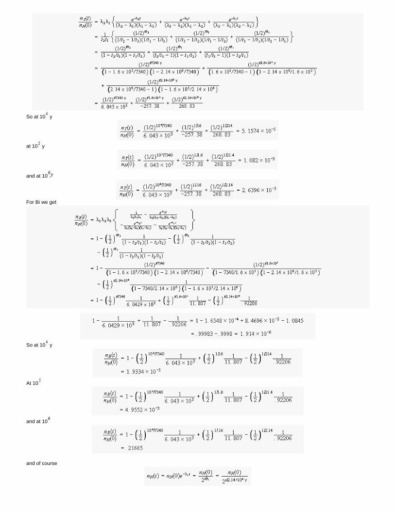
So at 10 y
at 10 y
and at 10
For Bi we get
So at 10 y
At 10
and at 10
and of course
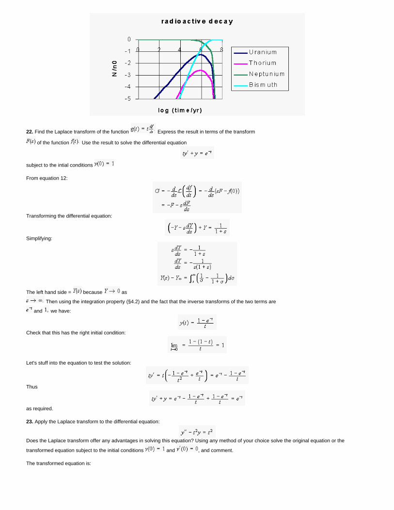
22. Find the Laplace transform of the function Express the result in terms of the transform
of the function Use the result to solve the differential equation
subject to the intial conditions
From equation 12:
Transforming the differential equation:
Simplifying:
The left hand side = because as
Then using the integration property (§4.2) and the fact that the inverse transforms of the two terms are
and we have:
Check that this has the right initial condition:
Let's stuff into the equation to test the solution:
Thus
as required.
23. Apply the Laplace transform to the differential equation:
Does the Laplace transform offer any advantages in solving this equation? Using any method of your choice solve the original equation or the
transformed equation subject to the initial conditions and , and comment.
The transformed equation is:
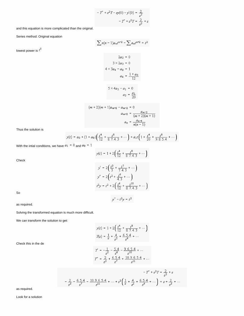
and this equation is more complicated than the original.
Series method: Original equation
lowest power is
Thus the solution is
With the intial conditions, we have and
Check
So
as required.
Solving the transformed equation is much more difficult.
We can transform the solution to get:
Check this in the de
as required.
Look for a solution
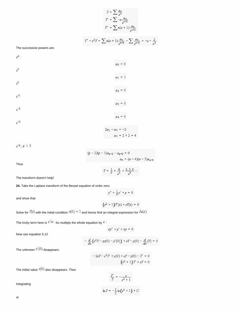
The successive powers are:
Thus
The transform doesn't help!
24. Take the Laplace transform of the Bessel equation of order zero
and show that
Solve for with the initial condition and hence find an integral expression for
The tricky term here is So multiply the whole equation by
Now use equation 5.12
The unknown disappears:
The initial value also disappears. Then
Integrating
or
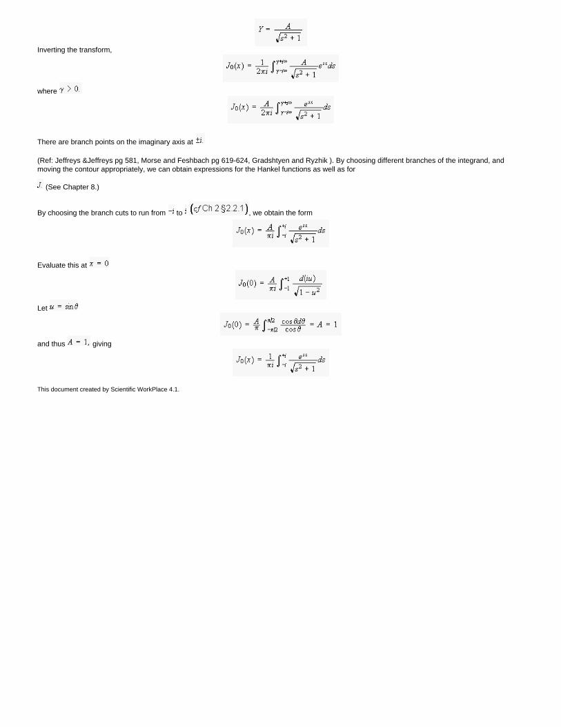
Inverting the transform,
where
There are branch points on the imaginary axis at
(Ref: Jeffreys &Jeffreys pg 581, Morse and Feshbach pg 619-624, Gradshtyen and Ryzhik ). By choosing different branches of the integrand, and moving the contour appropriately, we can obtain expressions for the Hankel functions as well as for
(See Chapter 8.)
By choosing the branch cuts to run from to , we obtain the form
Evaluate this at
Let
and thus giving
This document created by Scientific WorkPlace 4.1.
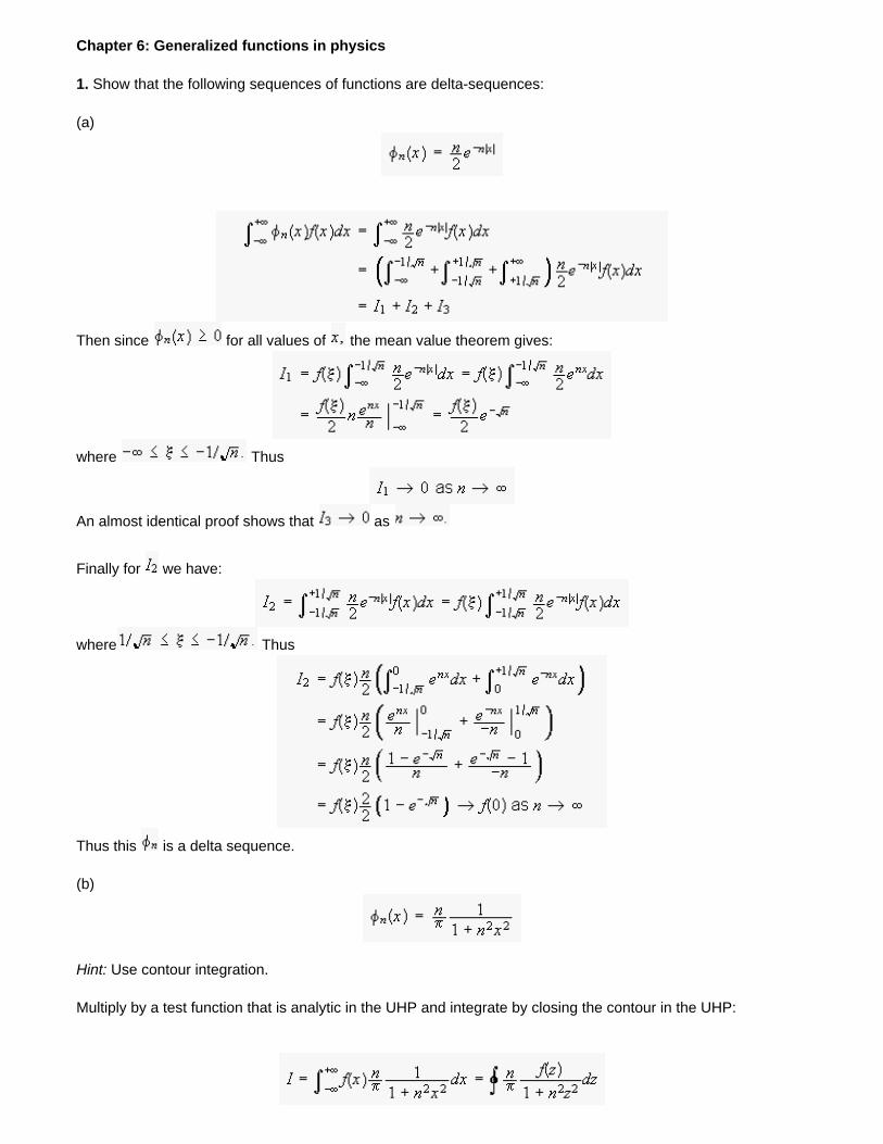
Chapter 6: Generalized functions in physics
1. Show that the following sequences of functions are delta-sequences:
(a)
Then since for all values of the mean value theorem gives:
where Thus
An almost identical proof shows that as
Finally for we have:
where Thus
Thus this is a delta sequence.
(b)
Hint: Use contour integration.
Multiply by a test function that is analytic in the UHP and integrate by closing the contour in the UHP:
The poles are at Only the pole at is inside the contour, so:
Thus in the limit:
which is the sifting property. Thus is a delta-sequence.
(c)
We evaluate
We evaluate along the real axis in the complex plane. We'll displace the path of integration downward so that it
lies beneath the (removable) singularity at Then we write the integral as:
Then provided that is analytic except for a set of poles, we have:
We close the contour upward for the first integral and downward for the second. In both cases the integral along the big semi-circle goes to zero, and we can use the residue theorem. For the first integral, the pole at
is inside the contour, and
(Note: the exponential is bounded because for poles in the upper-half plane.) Then:
For the second integral, the pole at is not inside the contour and the integral is zero in the limit. Thus
and the sifting property holds. Thus is a delta sequence.
2. Find a Fourier series representation of the delta function in the range in two ways.
(a) Start with the fourier series for a step function (cf equations 4.11 or 4.20) and differentiate.
The series (4.11) is a step function with a downward step at We modify it to give an upward step at
and a full period of Then the series we want is:
Now we take the derivative:
which is a series with constant coefficients, as we have come to expect.
(b) Start with the block functions (equation 6.2) and form the Fourier series. Take the limit as
Using the block functions:
where
and
Now we take the limit as
Are the results the same? If not, why not? Give a quantitative as well as a qualitative account of any discrepancy.
The results are not the same. The first result is a sum over only odd values of but its amplitude is twice that of the second result. We should not expect the results to be the same, because the first result gives a periodic
set of both positive and negative functions, positive at 2 etc and negative at 3 etc.
The second result gives a periodic repetition of positive functions at etc.
To verify this, let's take the second series, shift it by multiply by and add it to the original series. This should give the first series:
which is the first series, as expected.
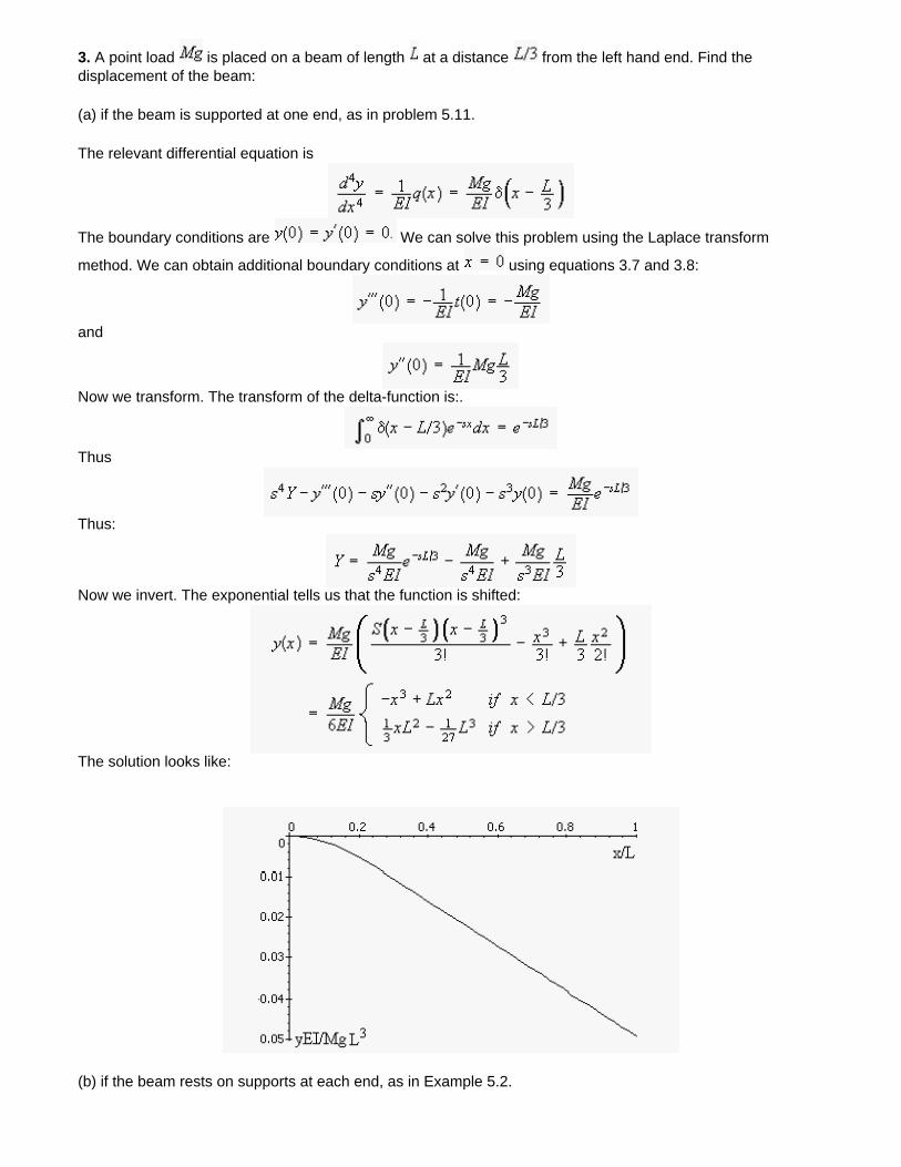
3. A point load is placed on a beam of length at a distance from the left hand end. Find the displacement of the beam:
(a) if the beam is supported at one end, as in problem 5.11.
The relevant differential equation is
The boundary conditions are We can solve this problem using the Laplace transform
method. We can obtain additional boundary conditions at using equations 3.7 and 3.8:
and
Now we transform. The transform of the delta-function is:.
Thus
Thus:
Now we invert. The exponential tells us that the function is shifted:
The solution looks like:
(b) if the beam rests on supports at each end, as in Example 5.2.
We have the same differential equation but different boundary conditions. Now Let's use a Fourier series:
Then
Thus the coefficients are given by:
and so
The series converges very fast because of the factor in the denominator. Every third term is missing
( for etc). The solution looks like:
4. A damped harmonic oscillator (cf Problem 4.13) has initial condistions and An
impulse is applied at Find the motion of the oscillator for .
We'll solve this using a Laplace transform:
Thus
Let's factor the denominator, and use the attenuation property:
Then, setting :
Inverting gives:
Thus for
while for
5. Distributions may be multiplied by infinitely differentiable functions. Do you expect the product
to be a valid distribution? Why or why not?
Not necessarily, because the function is not differentiable at . (Distributions may be multiplied by infinitely differentiable functions.)
Investigate the properties of this quantity by evaluating the integral
where is a delta sequence of your choice, and is a test function. In particular, determine the result
for functions that have the property Is a valid distribution in this case? Can you identify it?
We can evaluate the integral by using the Taylor series for about
All terms after the first two are zero in the limit The second gives The first is indeterminate
unless is a zero of In that case we may write:
Alternative proof: Use the block function delta-sequence:
Now let
Now if then we may add it:
This document created by Scientific WorkPlace 4.1.
Chapter 6: Generalized functions in physics
6. Evaluate
Since then
Thus
(b)
The delta function may be written:
and thus
7. A string of length with tension and mass per unit length is hit simultaneously at
at the two points and The impulse delivered at each point is Find the subsequent displacement of the string.
The initial conditions are and
The solution is then of the form
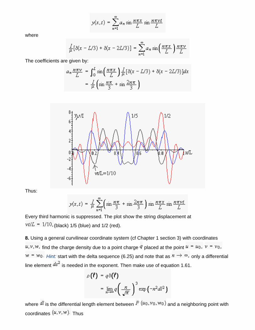
where
The coefficients are given by:
Thus:
Every third harmonic is suppressed. The plot show the string displacement at
(black) 1/5 (blue) and 1/2 (red).
8. Using a general curvilinear coordinate system (cf Chapter 1 section 3) with coordinates
find the charge density due to a point charge placed at the point
Hint: start with the delta sequence (6.25) and note that as only a differential
line element is needed in the exponent. Then make use of equation 1.61.
where is the differential length element between and a neighboring point with
coordinates Thus
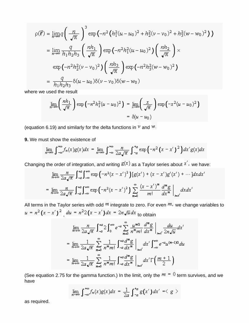
where we used the result
(equation 6.19) and similarly for the delta functions in and
9. We must show the existence of
Changing the order of integration, and writing as a Taylor series about we have:
All terms in the Taylor series with odd integrate to zero. For even we change variables to
, to obtain
(See equation 2.75 for the gamma function.) In the limit, only the term survives, and we have
as required.
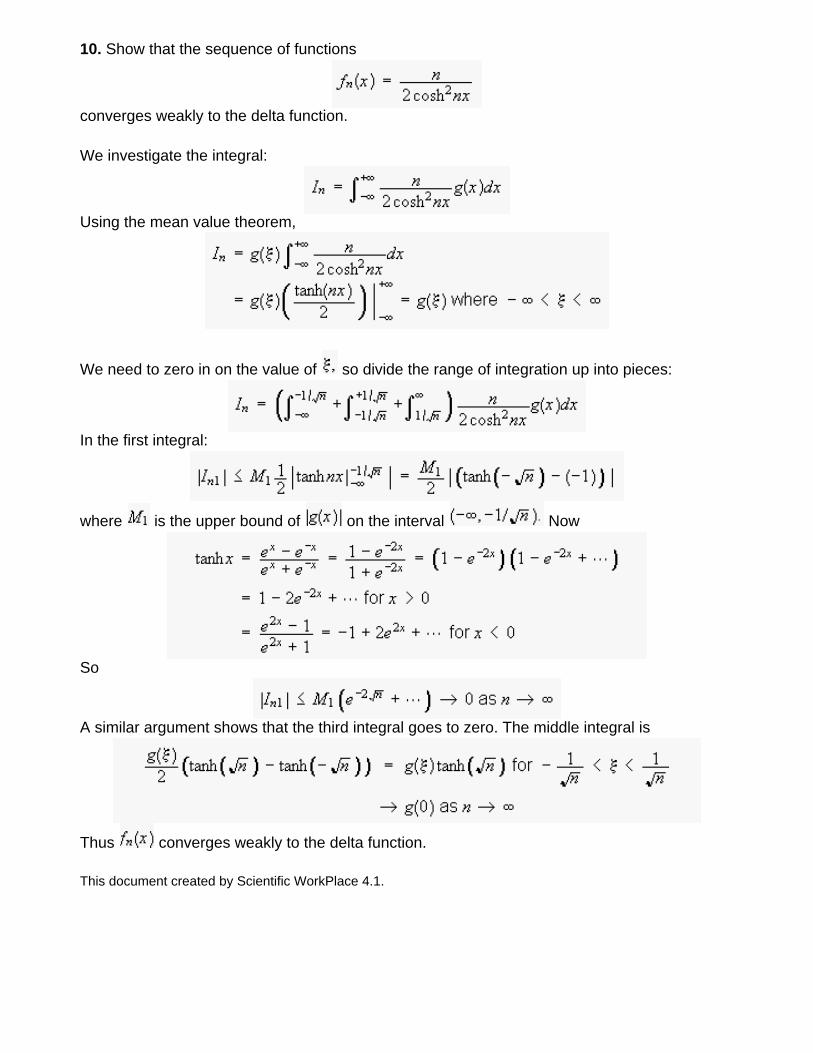
10. Show that the sequence of functions
converges weakly to the delta function.
We investigate the integral:
Using the mean value theorem,
We need to zero in on the value of so divide the range of integration up into pieces:
In the first integral:
where is the upper bound of on the interval Now
So
A similar argument shows that the third integral goes to zero. The middle integral is
Thus converges weakly to the delta function.
This document created by Scientific WorkPlace 4.1.
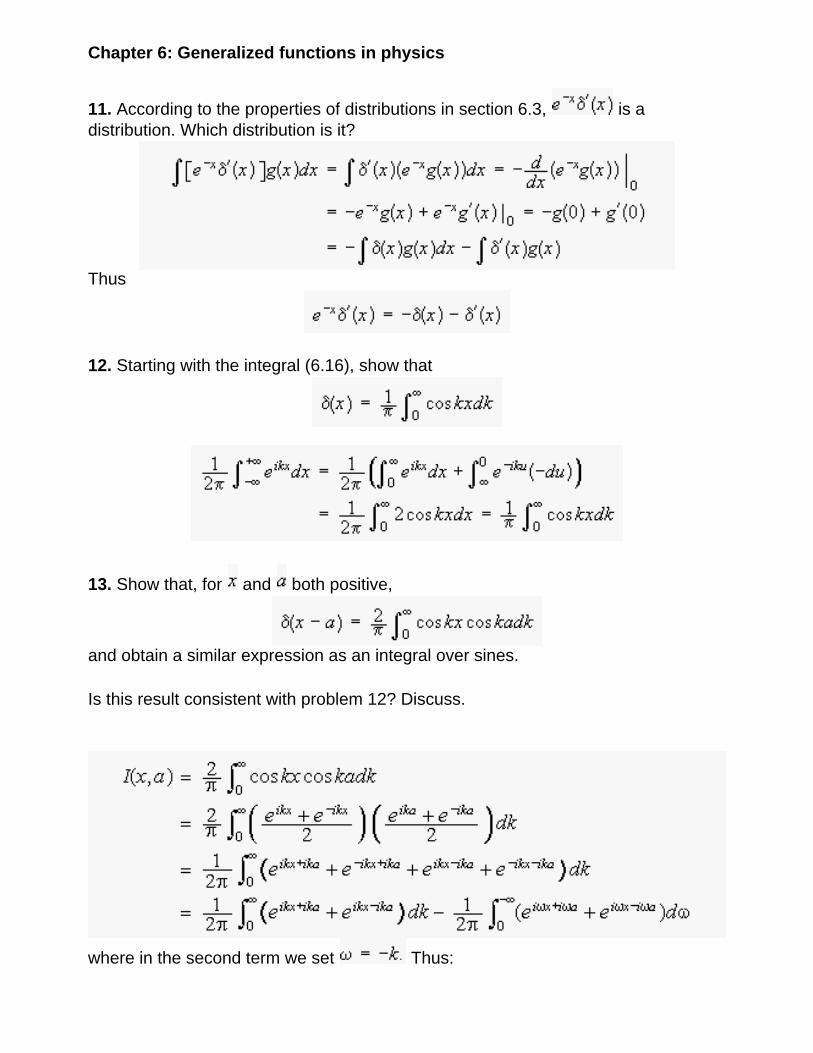
Chapter 6: Generalized functions in physics
11. According to the properties of distributions in section 6.3, is a distribution. Which distribution is it?
Thus
12. Starting with the integral (6.16), show that
13. Show that, for and both positive,
and obtain a similar expression as an integral over sines.
Is this result consistent with problem 12? Discuss.
where in the second term we set Thus:
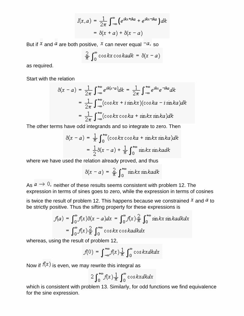
But if and are both positive, can never equal so
as required.
Start with the relation
The other terms have odd integrands and so integrate to zero. Then
where we have used the relation already proved, and thus
As neither of these results seems consistent with problem 12. The expression in terms of sines goes to zero, while the expression in terms of cosines
is twice the result of problem 12. This happens because we constrained and to be strictly positive. Thus the sifting property for these expressions is
whereas, using the result of problem 12,
Now if is even, we may rewrite this integral as
which is consistent with problem 13. Similarly, for odd functions we find equivalence for the sine expression.
14. Find the Laplace transform of Express the inverse as an integral using equation 5.19 and demonstrate that this integral possesses the sifting property.
Thus
So we check for the sifting property:
as required.
15. A disk of radius and mass lies in the plane. Express the density in terms of delta functions
(a) in rectangular Cartesian coordinates
In Cartesian coordinates, the disk is located at We have:
if and zero otherwise. We can also express this in terms of step functions:
(b) in cylindrical coordinates
In cylindrical coordinates, the step function looks nicer:
(c) in spherical coordinates.
The disk is at so the density looks like:
16. A rod of length and mass lies along the axis with one end at the origin. Determine the density using delta functions
(a) in rectangular Cartesian coordinates
The rod is restricted to and so we may write:
We may also write the result using step functions:
(b) in cylindrical coordinates
The rod is restricted to and We start with the result from part (a) and convert to cylindrical coordinates. In particular:
Thus:
Check the dimensions of the result!
(c) in spherical coordinates.
In spherical coordinates, the rod is at and The result must look like:
We need to find the function We integrate over a spherical shell with inner radius
and outer radius The amount of charge enclosed is Thus:
Now if is between 0 and we have:
Thus
and thus
This document created by Scientific WorkPlace 4.1.
Chapter 6: Generalized functions in physics
17. A line of charge with uniform line charge density lies along the axis. Find the volume charge density (a) in cylindrical coordinates and (b) in spherical coordinates.
(a)
The system has azimuthal symmetry, so there is no dependence on To find integrate over a cylindrical slice of
height
If did not depend on the result would be zero. Thus we must have Then
Thus and
(b) In spherical coordinates the charge exists only at and at Again there is no dependence on
This time we integrate over a spherical shell of radius This shell cuts the line at two places, so the charge
enclosed is 2
Here must have a factor in order that the result of the integration be non-zero. Thus
Thus
and
18. A disk of charge with radius and surface charge density lies in the plane with center at the origin. Find the volume charge density (a) in cylindrical coordinates and (b) in spherical coordinates.
(a)
Integrating over a wedge of a cylindrical shell at
Thus and
(b)
and integrating over an orange wedge shell at we get
Thus
and
19. Current flows in a loop of radius lying in the plane with its center at the origin. Find an expression for the current density (a) in cylindrical coordinates and (b) in spherical coordinates.
(a)
(b) The current exists only at and Thus
20. Prove the relation (equation 6.27)
where is the radial coordinate in a cylindrical coordinate system, and is the position vector in a plane.
For
For the derivatives cannot be computed. So we check for the sifting property:
as required.
Use the result to find the potential due to a line charge running parallel to the axis at
First we put the axis along the line occupied by the charge. The charge density in these coordinates is:
Then the equation satisfied by the potential is
Using the result above, we thus conclude that:
where here is the distance from the origin to the reference point where we choose to be zero. Then converting back to the original coordinates:
21. A circuit contains a resistor, a capacitor, and a square wave power supply with period Use Kirchhoff's loop rule to write an equation for the current in the circuit in terms of delta-functions, and solve it to find the current as a function of time.
Differentiate to get:
The term on the left is a sequence of functions, up at and down at etc Using equation 6.13
Then applying Kirchhoff's loop rule, we have
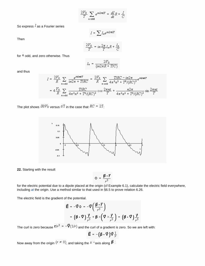
So express as a Fourier series
Then
for odd, and zero otherwise. Thus
and thus
The plot shows versus in the case that :
22. Starting with the result
for the electric potential due to a dipole placed at the origin (cf Example 6.1), calculate the electric field everywhere, including at the origin. Use a method similar to that used in §6.5 to prove relation 6.26.
The electric field is the gradient of the potential.
The curl is zero because and the curl of a gradient is zero. So we are left with:
Now away from the origin , and taking the axis along
However, at the origin, the derivatives cannot be computed in the usual way. Since we already know that
we should suspect the presence of a delta-function in this case too. We can check this assertion
by testing for the sifting property. We integrate over a small sphere of radius surrounding the origin:
All other components are zero. Then:
whereas, using the explicit form (6.1 solutions) we get:
To make these two results consistent, we must add a delta-function:
23. Using a delta-sequence of your choice, show that the limit
exhibits the sifting property of
which is the sifting property of
24. Use the derivative property 6.20 to show that, for distributions, the Laplace transform of the derivative
equals times the Laplace transform of Show that the Laplace transform of is where is Euler's
constant, Hence show that the Laplace transform of ( condsidered as a
distribution, is
Here is Maple verifying the value of by numerical integration:
Now
Then by the derivative rule, and thus
This document created by Scientific WorkPlace 4.1.
Chapter 6: Generalized functions in physics
25. Starting from equation 6.16, show that
Confirm your result by demonstrating the sifting property. Use contour integration to do the integral.
Similarly, show that
if the integral
is taken to be the principal value.
Demonstrate the plausibility of the results by evaluating and
numerically for a set of values of and Show that as increases, and decreases toward zero.
To check for the sifting property, we multiply by a test function that has a set of simple poles in the upper-half plane, and is analytic in the lower half plane. Then integrate.
Close the contour upward for the first term and downward for the second term. There is a pole at
Putting a little semicircle under the pole, we get
Then as
because is positive. Thus
The result is the same if we put the semicicrle over the pole at the origin, as it must be, since
has a removable singularity at .
Replacing the sine with a cosine, the pole is not removable, and the result depends on how the path is chosen. The principal value is zero. Putting the semicircle under the pole:
Thus
Now for some numerical integration: First the sine.
The results approach 1.
For the cosine, we have:
The plot shows versus The integral approaches zero as increases.
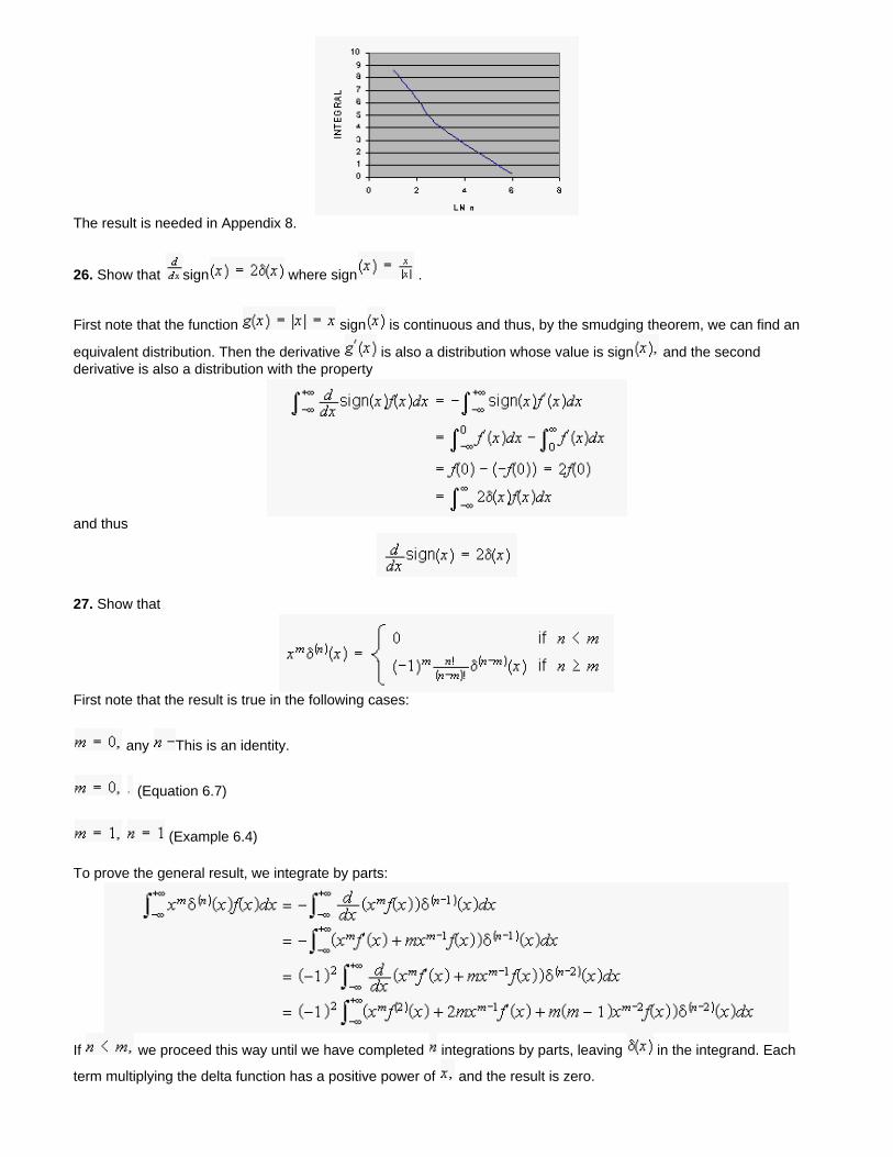
The result is needed in Appendix 8.
26. Show that sign where sign .
First note that the function sign is continuous and thus, by the smudging theorem, we can find an
equivalent distribution. Then the derivative is also a distribution whose value is sign and the second derivative is also a distribution with the property
and thus
27. Show that
First note that the result is true in the following cases:
any This is an identity.
(Equation 6.7)
(Example 6.4)
To prove the general result, we integrate by parts:
If we proceed this way until we have completed integrations by parts, leaving in the integrand. Each
term multiplying the delta function has a positive power of and the result is zero.
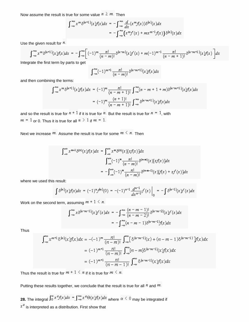
Now assume the result is true for some value Then
Use the given result for
Integrate the first term by parts to get
and then combining the terms:
and so the result is true for if it is true for But the result is true for , with
or 0. Thus it is true for all if
Next we increase Assume the result is true for some Then
where we used this result:
Work on the second term, assuming
Thus
Thus the result is true for if it is true for
Putting these results together, we conclude that the result is true for all and
28. The integral . where may be integrated if
is interpreted as a distribution. First show that
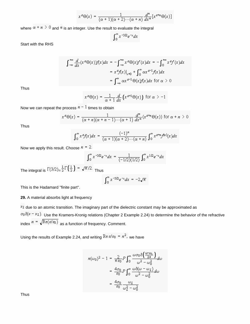
where and is an integer. Use the result to evaluate the integral
Start with the RHS
Thus
Now we can repeat the process times to obtain
Thus
Now we apply this result. Choose
The integral is = Thus
This is the Hadamard ''finite part''.
29. A material absorbs light at frequency
due to an atomic transition. The imaginary part of the dielectric constant may be approximated as
Use the Kramers-Kronig relations (Chapter 2 Example 2.24) to determine the behavior of the refractive
index as a function of frequency. Comment.
Using the results of Example 2.24, and writing we have
Thus
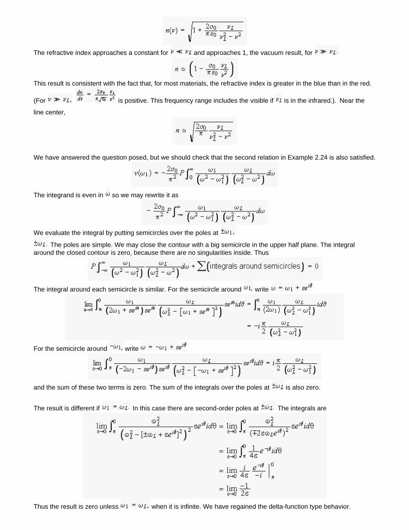
The refractive index approaches a constant for and approaches 1, the vacuum result, for
This result is consistent with the fact that, for most materials, the refractive index is greater in the blue than in the red.
(For is positive. This frequency range includes the visible if is in the infrared.). Near the
line center,
We have answered the question posed, but we should check that the second relation in Example 2.24 is also satisfied.
The integrand is even in so we may rewrite it as
We evaluate the integral by putting semicircles over the poles at
The poles are simple. We may close the contour with a big semicircle in the upper half plane. The integral around the closed contour is zero, because there are no singularities inside. Thus
The integral around each semicircle is similar. For the semicircle around write
For the semicircle around write
and the sum of these two terms is zero. The sum of the integrals over the poles at is also zero.
The result is different if In this case there are second-order poles at The integrals are
Thus the result is zero unless when it is infinite. We have regained the delta-function type behavior.
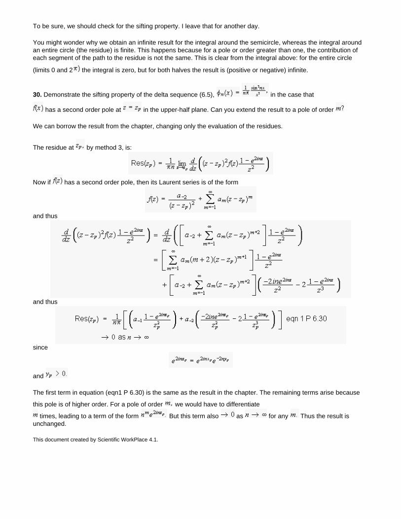
To be sure, we should check for the sifting property. I leave that for another day.
You might wonder why we obtain an infinite result for the integral around the semicircle, whereas the integral around an entire circle (the residue) is finite. This happens because for a pole or order greater than one, the contribution of each segment of the path to the residue is not the same. This is clear from the integral above: for the entire circle
(limits 0 and 2 the integral is zero, but for both halves the result is (positive or negative) infinite.
30. Demonstrate the sifting property of the delta sequence (6.5), in the case that
has a second order pole at in the upper-half plane. Can you extend the result to a pole of order
We can borrow the result from the chapter, changing only the evaluation of the residues.
The residue at by method 3, is:
Now if has a second order pole, then its Laurent series is of the form
and thus
and thus
since
and
The first term in equation (eqn1 P 6.30) is the same as the result in the chapter. The remaining terms arise because
this pole is of higher order. For a pole of order we would have to differentiate
times, leading to a term of the form But this term also as for any Thus the result is unchanged.
This document created by Scientific WorkPlace 4.1.
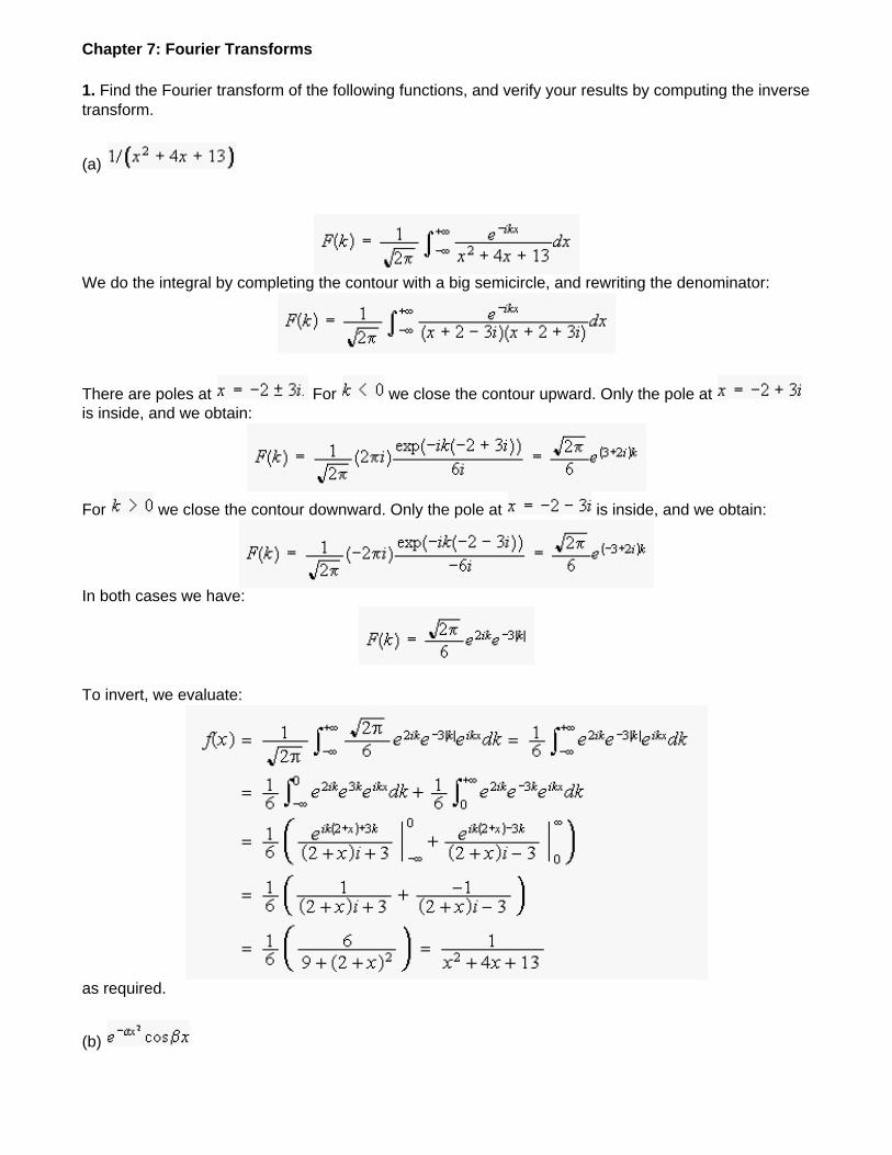
Chapter 7: Fourier Transforms
1. Find the Fourier transform of the following functions, and verify your results by computing the inverse transform.
(a)
We do the integral by completing the contour with a big semicircle, and rewriting the denominator:
There are poles at For we close the contour upward. Only the pole at is inside, and we obtain:
For we close the contour downward. Only the pole at is inside, and we obtain:
In both cases we have:
To invert, we evaluate:
as required.
(b)
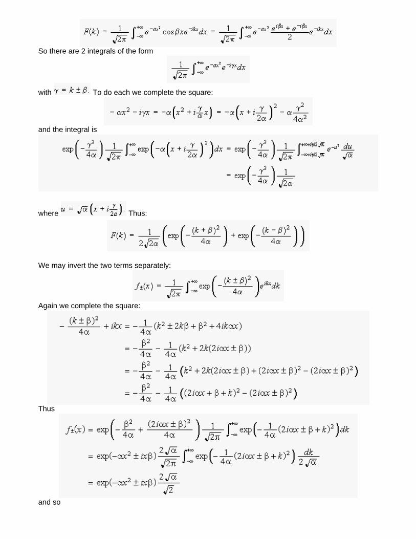
So there are 2 integrals of the form
with To do each we complete the square:
and the integral is
where Thus:
We may invert the two terms separately:
Again we complete the square:
Thus
and so
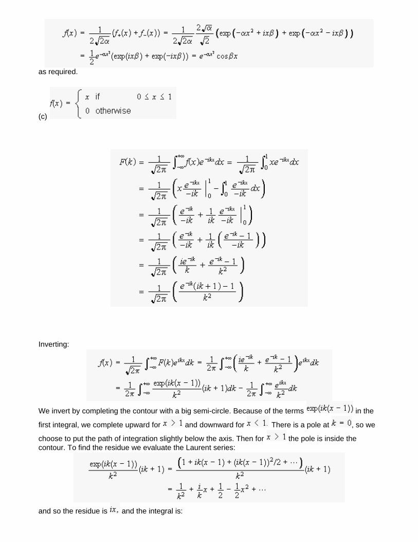
as required.
(c)
Inverting:
We invert by completing the contour with a big semi-circle. Because of the terms in the
first integral, we complete upward for and downward for There is a pole at , so we
choose to put the path of integration slightly below the axis. Then for the pole is inside the contour. To find the residue we evaluate the Laurent series:
and so the residue is and the integral is:
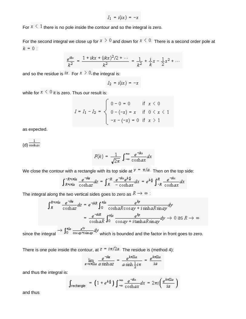
For there is no pole inside the contour and so the integral is zero.
For the second integral we close up for and down for There is a second order pole at
and so the residue is For the integral is:
while for it is zero. Thus our result is:
as expected.
(d)
We close the contour with a rectangle with its top side at Then on the top side:
The integral along the two vertical sides goes to zero as
since the integral which is bounded and the factor in front goes to zero.
There is one pole inside the contour, at The residue is (method 4):
and thus the integral is:
and thus
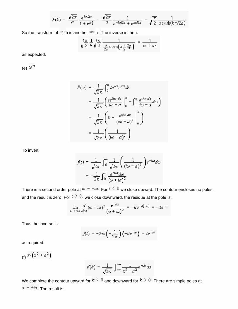
So the transform of h is another h The inverse is then:
as expected.
(e)
To invert:
There is a second order pole at For we close upward. The contour encloses no poles,
and the result is zero. For we close downward. the residue at the pole is:
Thus the inverse is:
as required.
(f)
We complete the contour upward for and downward for There are simple poles at
The result is:
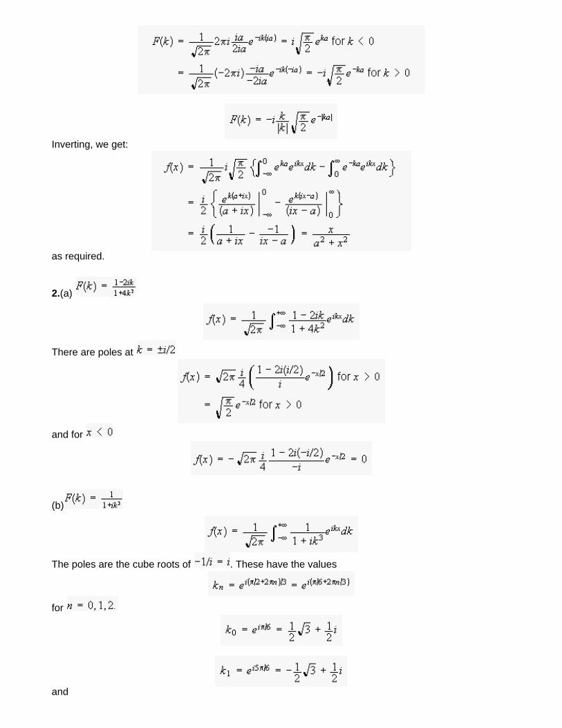
Inverting, we get:
as required.
2.(a)
There are poles at
and for
(b)
The poles are the cube roots of . These have the values
for
and
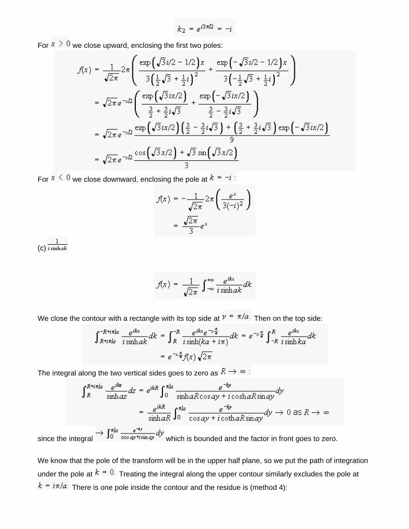
For we close upward, enclosing the first two poles:
For we close downward, enclosing the pole at
(c)
We close the contour with a rectangle with its top side at Then on the top side:
The integral along the two vertical sides goes to zero as
since the integral which is bounded and the factor in front goes to zero.
We know that the pole of the transform will be in the upper half plane, so we put the path of integration
under the pole at Treating the integral along the upper contour similarly excludes the pole at
There is one pole inside the contour and the residue is (method 4):
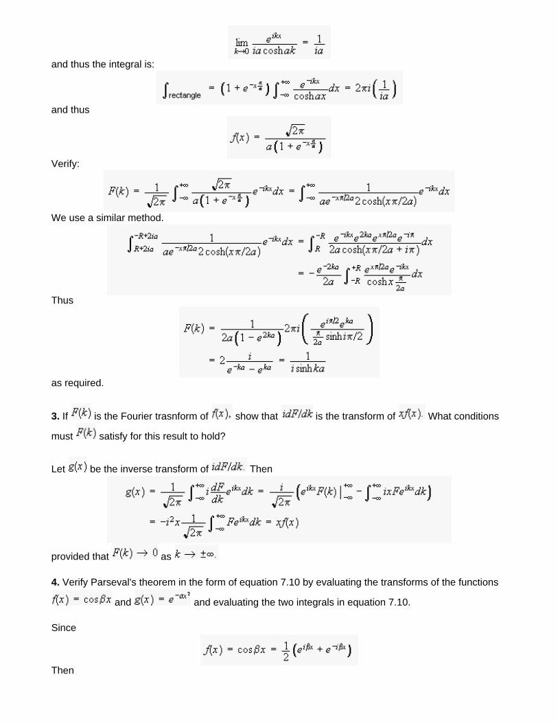
and thus the integral is:
and thus
Verify:
We use a similar method.
Thus
as required.
3. If is the Fourier trasnform of show that is the transform of What conditions
must satisfy for this result to hold?
Let be the inverse transform of Then
provided that as
4. Verify Parseval's theorem in the form of equation 7.10 by evaluating the transforms of the functions
and and evaluating the two integrals in equation 7.10.
Since
Then
and from Example 7.2
Then
We also need
and then from the result of Example 7.2:
and the two integrals are equal, as required.
5. Verify Parseval's theorem in the form of equation 7.11 by evaluating the transform of
and evaluating the integrals of and
Then
and
We can most easily do the integrals by dividing into 2 pieces and closing the contour separately for each piece:
Each integrand then has a first order pole at We displace the contour down by a small amount so as to pass beneath the pole. Then:
and Parseval's theorem is verified for this function.
This document created by Scientific WorkPlace 4.1.
Chapter 7: Fourier Transforms
6. Show that if is the transform of then is the transform of Show that the result is consistent with Parseval's theorem.
Parseval's theorem states:
Now for we have:
where is the transform of On the left hand side, change variables to and on the right
change variables to
Thus
as required.
7. Find the Fourier transform of the function that represents a
finite train of data. Plot the Fourier power spectrum as a function of for the two cases and
and comment. What happens as increases toward infinity?
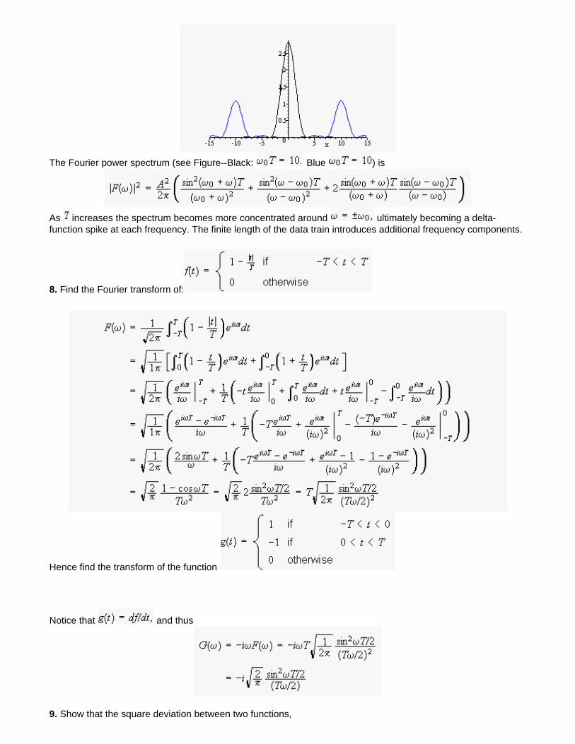
The Fourier power spectrum (see Figure--Black: Blue ) is
As increases the spectrum becomes more concentrated around ultimately becoming a delta-function spike at each frequency. The finite length of the data train introduces additional frequency components.
8. Find the Fourier transform of:
Hence find the transform of the function
Notice that and thus
9. Show that the square deviation between two functions,
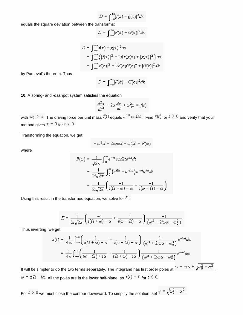
equals the square deviation between the transforms:
by Parseval's theorem. Thus
10. A spring- and -dashpot system satisfies the equation
with The driving force per unit mass equals Find for and verify that your
method gives for
Transforming the equation, we get:
where
Using this result in the transformed equation, we solve for
Thus inverting, we get:
It will be simpler to do the two terms separately. The integrand has first order poles at ,
All the poles are in the lower half-plane, so for
For we must close the contour downward. To simplify the solution, set
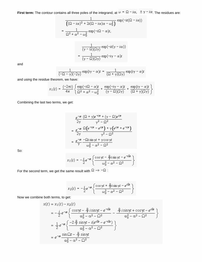
First term: The contour contains all three poles of the integrand, at . The residues are:
and
and using the residue theorem, we have:
Combining the last two terms, we get:
So:
For the second term, we get the same result with
Now we combine both terms, to get:
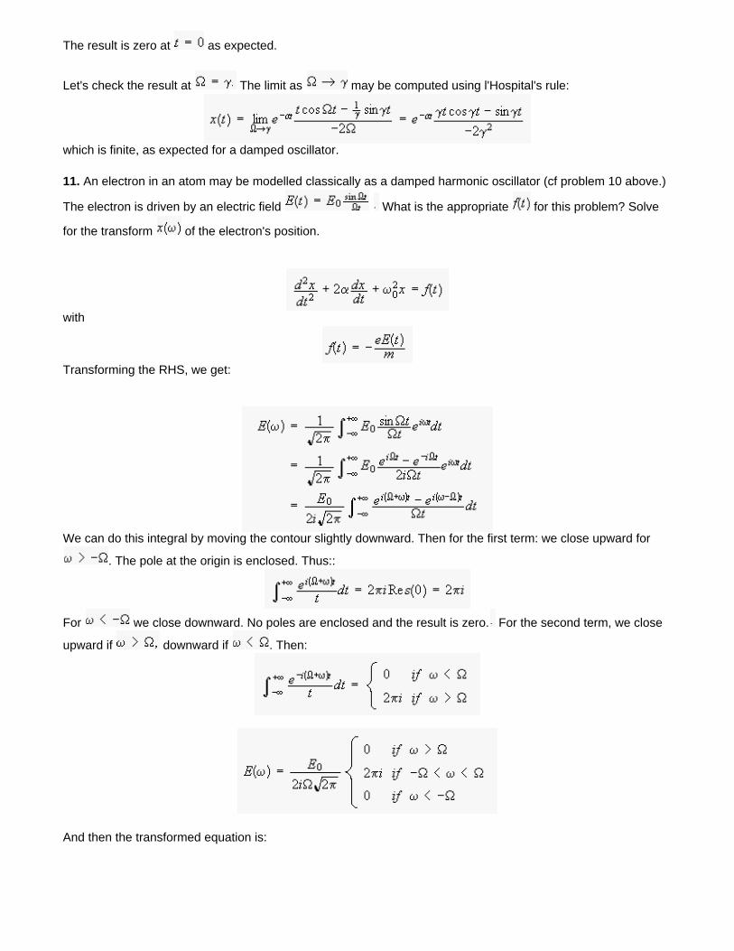
The result is zero at as expected.
Let's check the result at The limit as may be computed using l'Hospital's rule:
which is finite, as expected for a damped oscillator.
11. An electron in an atom may be modelled classically as a damped harmonic oscillator (cf problem 10 above.)
The electron is driven by an electric field What is the appropriate for this problem? Solve
for the transform of the electron's position.
with
Transforming the RHS, we get:
We can do this integral by moving the contour slightly downward. Then for the first term: we close upward for
. The pole at the origin is enclosed. Thus::
For we close downward. No poles are enclosed and the result is zero. For the second term, we close
upward if downward if . Then:
And then the transformed equation is:
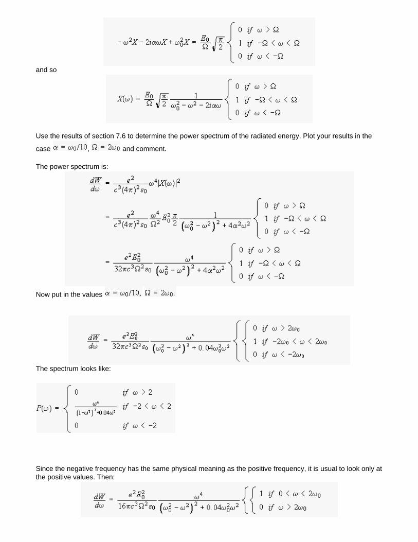
and so
Use the results of section 7.6 to determine the power spectrum of the radiated energy. Plot your results in the
case , and comment.
The power spectrum is:
Now put in the values
The spectrum looks like:
Since the negative frequency has the same physical meaning as the positive frequency, it is usual to look only at the positive values. Then:
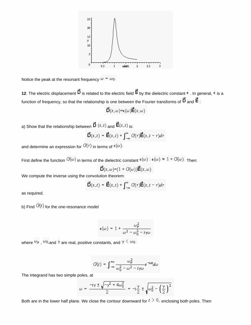
Notice the peak at the resonant frequency
12. The electric displacement is related to the electric field by the dielectric constant . In general, is a
function of frequency, so that the relationship is one between the Fourier transforms of and :
a) Show that the relationship between and is:
and determine an expression for in terms of
First define the function in terms of the dielectric constant Then:
We compute the inverse using the convolution theorem:
as required.
b) Find for the one-resonance model
where , and are real, positive constants, and
The integrand has two simple poles, at
Both are in the lower half plane. We close the contour downward for enclosing both poles. Then
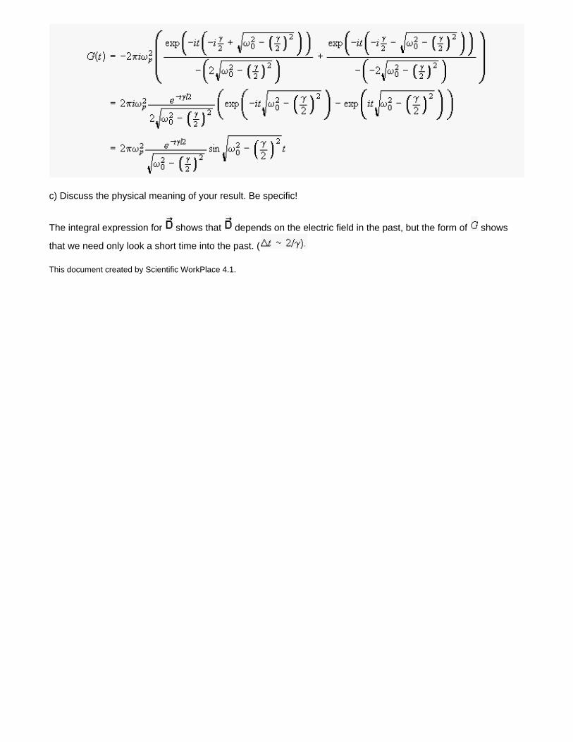
c) Discuss the physical meaning of your result. Be specific!
The integral expression for shows that depends on the electric field in the past, but the form of shows
that we need only look a short time into the past. (
This document created by Scientific WorkPlace 4.1.
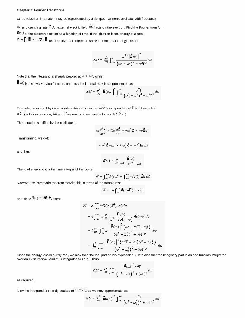
Chapter 7: Fourier Transforms
13. An electron in an atom may be represented by a damped harmonic oscillator with frequency
and damping rate . An external electric field acts on the electron. Find the Fourier transform
of the electron position as a function of time. If the electron loses energy at a rate
, use Parseval's Theorem to show that the total energy loss is:
Note that the integrand is sharply peaked at , while
is a slowly varying function, and thus the integral may be approximated as:
Evaluate the integral by contour integration to show that is independent of and hence find
. (In this expression, and are real positive constants, and .)
The equation satsified by the oscillator is:
Transforming, we get:
and thus
The total energy lost is the time integral of the power:
Now we use Parseval's theorem to write this in terms of the transforms:
and since then:
Since the energy loss is purely real, we may take the real part of this expression. (Note also that the imaginary part is an odd function integrated over an even interval, and thus integrates to zero.) Thus:
as required.
Now the integrand is sharply peaked at so we may approximate as:
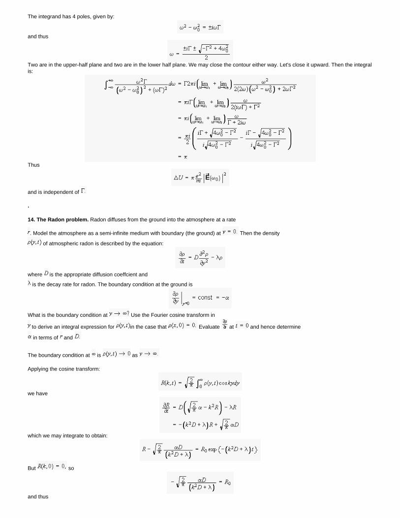
The integrand has 4 poles, given by:
and thus
Two are in the upper-half plane and two are in the lower half plane. We may close the contour either way. Let's close it upward. Then the integral is:
Thus
and is independent of
.
14. The Radon problem. Radon diffuses from the ground into the atmosphere at a rate
. Model the atmosphere as a semi-infinite medium with boundary (the ground) at Then the density
of atmospheric radon is described by the equation:
where is the appropriate diffusion coeffcient and
is the decay rate for radon. The boundary condition at the ground is
What is the boundary condition at Use the Fourier cosine transform in
to derive an integral expression for in the case that Evaluate at and hence determine
in terms of and
The boundary condition at is as
Applying the cosine transform:
we have
which we may integrate to obtain:
But so
and thus
Now differentiating, we get
Thus
Let Then and
where is the error function.
Also note
Then:
After a long time: (G&R 3.471#9 with
and for large this takes the form
We can also use equation (Radon eqn 1) to get the long time solution:
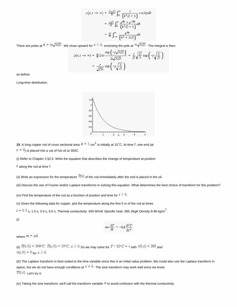
There are poles at We close upward for enclosing the pole at The integral is then:
as before.
Long-time distribution.
15. A long copper rod of cross sectional area cm is initially at 15 C. At time , one end (at
) is placed into a vat of hot oil at 300C.
(i) Refer to Chapter 3 §2.5. Write the equation that describes the change of temperature at position
along the rod at time .
(ii) Write an expression for the temperature of the rod immediately after the end is placed in the oil.
(iii) Discuss the use of Fourier and/or Laplace transforms in solving this equation. What determines the best choice of transform for this problem?
(iv) Find the temperature of the rod as a function of position and time for .
(v) Given the following data for copper, plot the temperature along the first 5 m of the rod at times
s, 1.5 s, 3.0 s, 6.0 s. Thermal conductivity: 400 W/mK Specific heat: 385 J/kgK Density 8.96 kg/m .
(i)
where
(ii) So we may solve for with and
for
(iii) The Laplace transform is best suited to the time variable since this is an initial value problem. We could also use the Laplace transform in
space, but we do not have enough conditions at The sine transform may work well since we know
Let's try it.
(iv) Taking the sine transform, we'll call the transform variable to avoid confusion with the thermal conductivity.
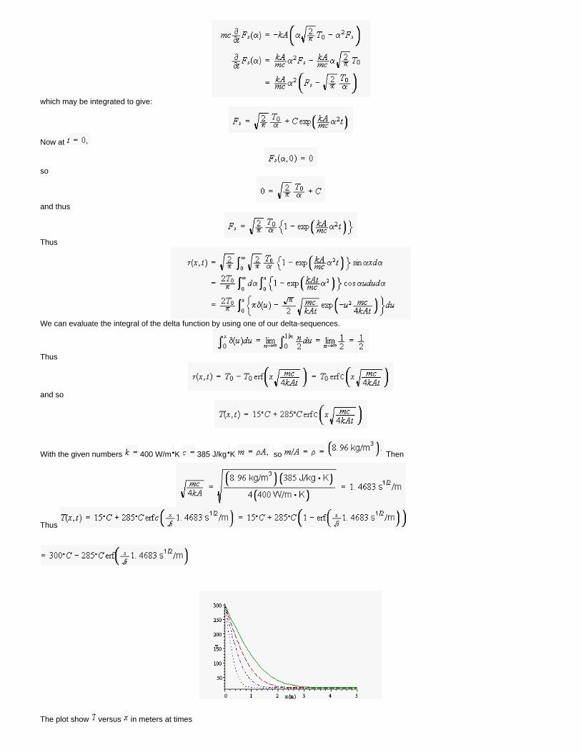
which may be integrated to give:
Now at
so
and thus
Thus
We can evaluate the integral of the delta function by using one of our delta-sequences.
Thus
and so
With the given numbers 400 W/m K 385 J/kg K so Then
Thus
The plot show versus in meters at times
s (black, dotted line), 1.5 s (blue,dot-dash line), 3 s (red dashed line) and 6 s (green line).
16. A long beam is resting on an elastic foundation. The equation satisfied by the beam displacement is:
where is the load and
is a constant describing the elastic properties of the foundation. If the load is concentrated toward the center of the beam, then we may
assume that as Transform the equation, and find in terms of
Solve for the beam displacement if
(a) and
(b)
thus
(a)
Then
and
We integrate by completing the contour (upward for and downward for There are poles at
and two poles lie inside each contour. Write
Then for we close upward, enclosing the poles at The residues are:
and
Thus for :
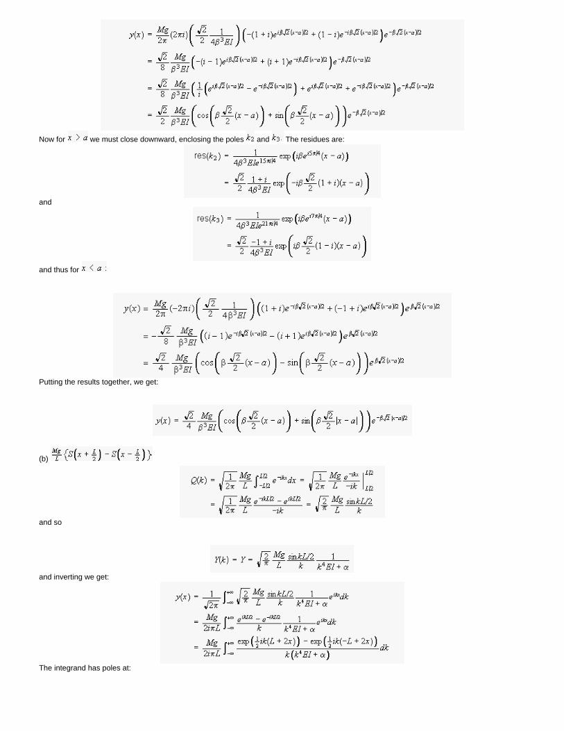
Now for we must close downward, enclosing the poles and The residues are:
and
and thus for
Putting the results together, we get:
(b)
and so
and inverting we get:
The integrand has poles at:
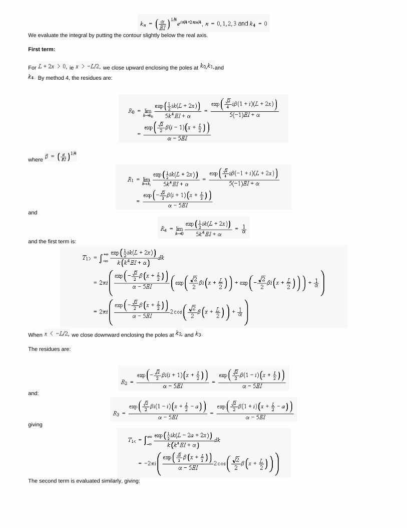
We evaluate the integral by putting the contour slightly below the real axis.
First term:
For ie we close upward enclosing the poles at and
By method 4, the residues are:
where
and
and the first term is:
When we close downward enclosing the poles at and
The residues are:
and:
giving
The second term is evaluated similarly, giving:
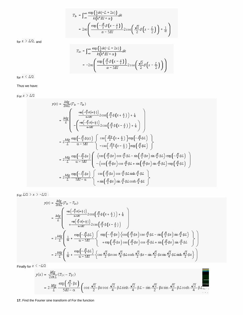
for and
for
Thus we have:
For
For
Finally for
17. Find the Fourier sine transform of For the function
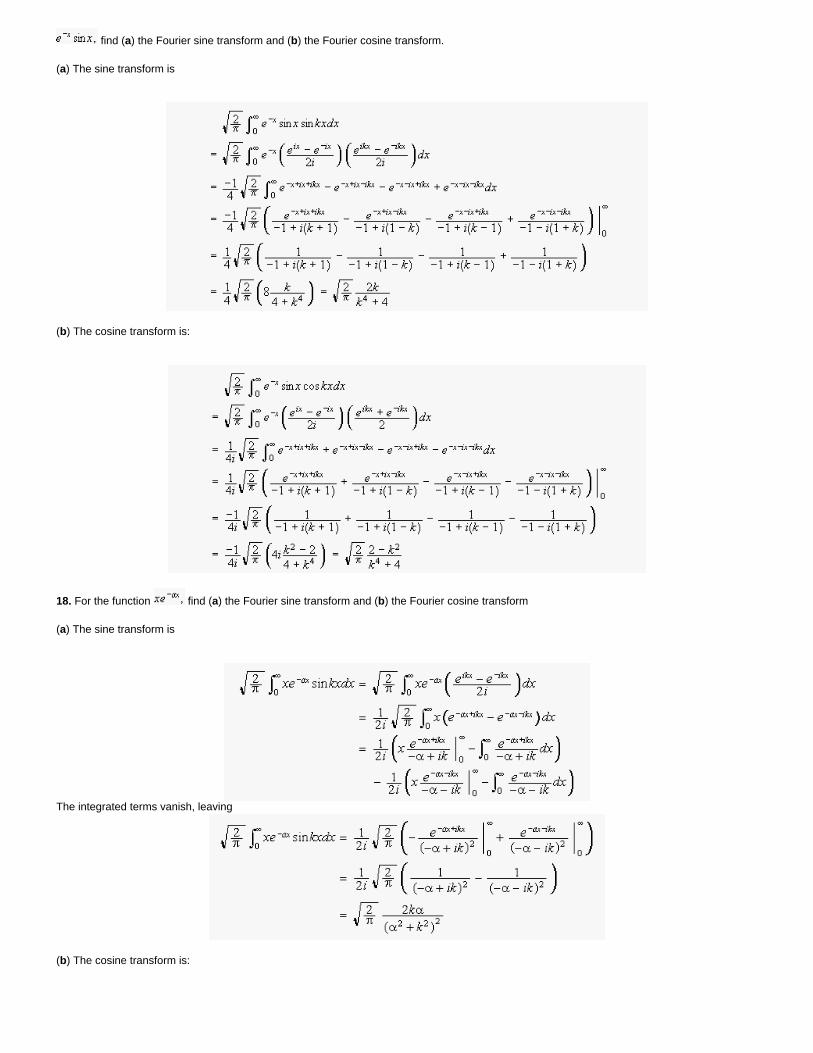
find (a) the Fourier sine transform and (b) the Fourier cosine transform.
(a) The sine transform is
(b) The cosine transform is:
18. For the function find (a) the Fourier sine transform and (b) the Fourier cosine transform
(a) The sine transform is
The integrated terms vanish, leaving
(b) The cosine transform is:
The integrated terms vanish, leaving
19. Show that the Fourier cosine transform of the function for is
Hence show that the function
is its own cosine transform. Obtain similar results for the sine transform. (The results of Chapter 2 §9 may prove useful.)
In the first term let and in the second let
where we can move both integrals to the real axis since there are no poles between the imagnary axis and the real axis.
In the special case w e find
so this function is its own transform.
The sine transform is
so that with we obtain the same result as for the cosine transform.
20. Determine the form of Parseval's theorem (equation 7.10 and 7.11) that applies to the cosine transform.
Following the method in section 7.3.5, and remembering that the functions are defined only for positive :
Then from the result of Problem 6.13,
The same expression holds for the sine transform.
The equivalent relation to 7.11 is thus:
This document created by Scientific WorkPlace 4.1.
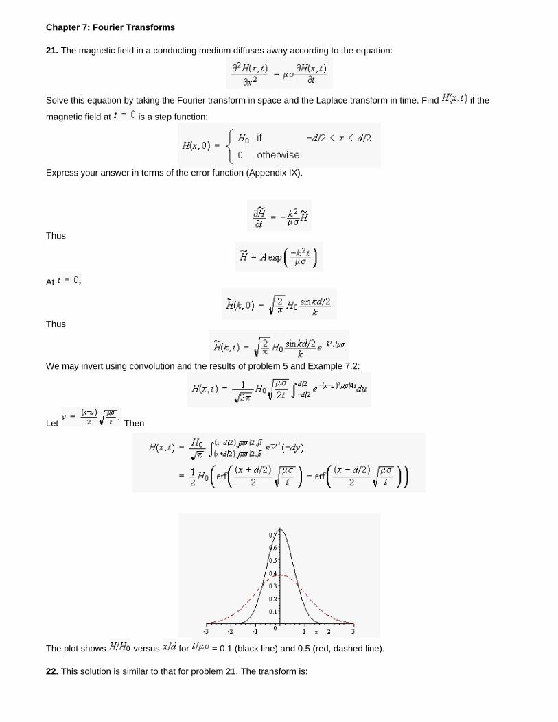
Chapter 7: Fourier Transforms
21. The magnetic field in a conducting medium diffuses away according to the equation:
Solve this equation by taking the Fourier transform in space and the Laplace transform in time. Find if the
magnetic field at is a step function:
Express your answer in terms of the error function (Appendix IX).
Thus
At
Thus
We may invert using convolution and the results of problem 5 and Example 7.2:
Let Then
The plot shows versus for = 0.1 (black line) and 0.5 (red, dashed line).
22. This solution is similar to that for problem 21. The transform is:
where
(Example 7.2 with Thus
and thus
23. Develop a three-dimensional version of the convolution theorem. Use the result to obtain the solution of Poisson's equation
Evaluate the resulting integral explicitly if
If the transform is of the form then
The transformed equation is:
Now the function inverts to
The integral has a simple pole at the origin. With
positive, we close upward with a small semicircle over the pole and a big semicircle at Then
The integral around the closed curve is zero by Cauchy's theorem ,and so the principle value is the negative of the
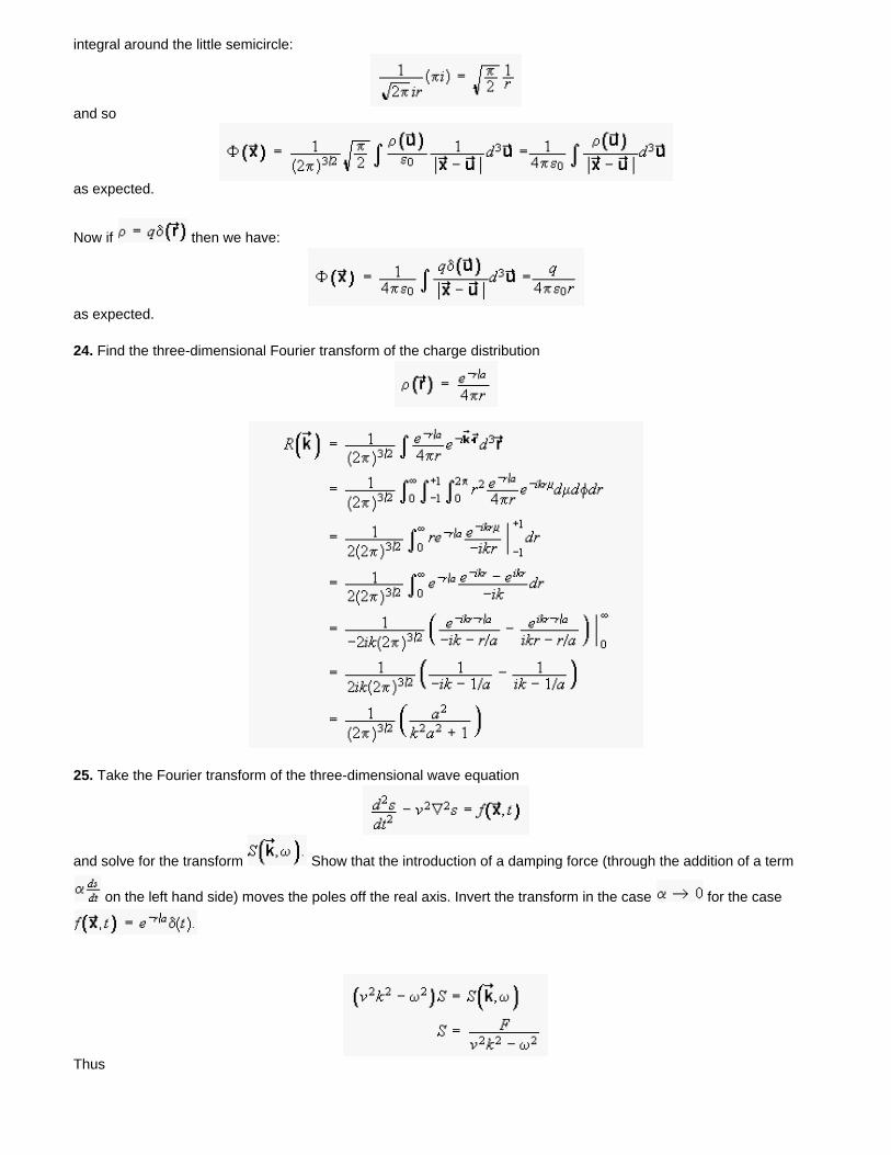
integral around the little semicircle:
and so
as expected.
Now if then we have:
as expected.
24. Find the three-dimensional Fourier transform of the charge distribution
25. Take the Fourier transform of the three-dimensional wave equation
and solve for the transform Show that the introduction of a damping force (through the addition of a term
on the left hand side) moves the poles off the real axis. Invert the transform in the case for the case
Thus
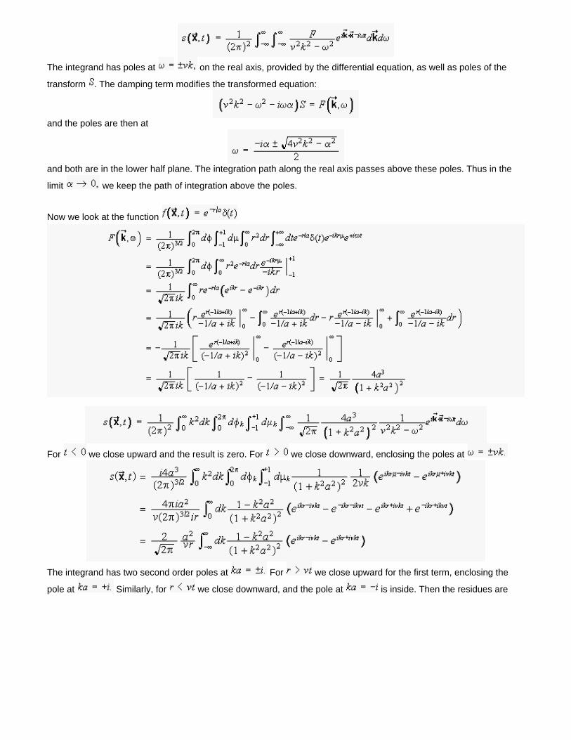
The integrand has poles at on the real axis, provided by the differential equation, as well as poles of the
transform . The damping term modifies the transformed equation:
and the poles are then at
and both are in the lower half plane. The integration path along the real axis passes above these poles. Thus in the
limit we keep the path of integration above the poles.
Now we look at the function
For we close upward and the result is zero. For we close downward, enclosing the poles at
The integrand has two second order poles at For we close upward for the first term, enclosing the
pole at Similarly, for we close downward, and the pole at is inside. Then the residues are
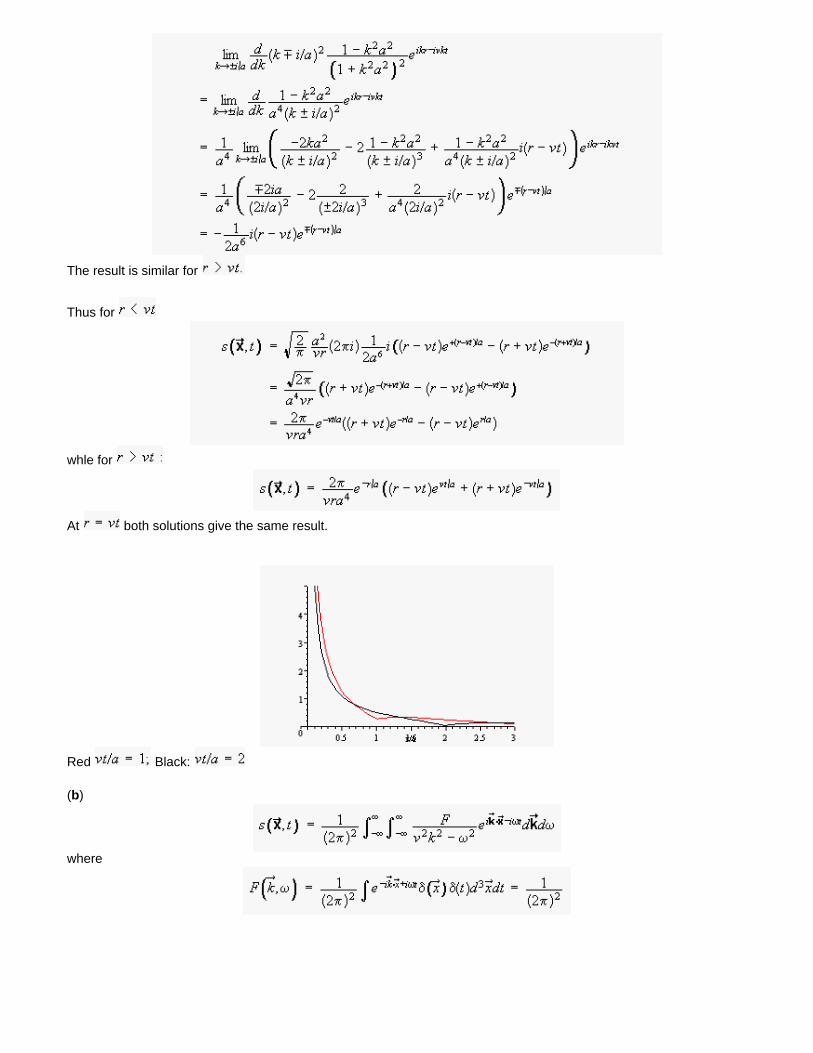
The result is similar for
Thus for
whle for
At both solutions give the same result.
Red Black:
(b)
where
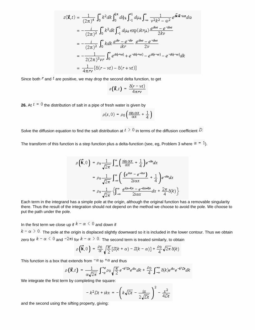
Since both and are positive, we may drop the second delta function, to get
26. At the distribution of salt in a pipe of fresh water is given by
Solve the diffusion equation to find the salt distribution at in terms of the diffusion coefficient
The transform of this function is a step function plus a delta-function (see, eg, Problem 3 where ).
Each term in the integrand has a simple pole at the origin, although the original function has a removable singularity there. Thus the result of the integration should not depend on the method we choose to avoid the pole. We choose to put the path under the pole.
In the first term we close up if and down if
The pole at the origin is displaced slightly downward so it is included in the lower contour. Thus we obtain
zero for and for The second term is treated similarly, to obtain
This function is a box that extends from to and thus
We integrate the first term by completing the square:
and the second using the sifting property, giving:
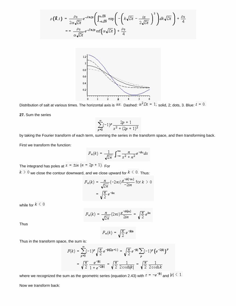
Distribution of salt at various times. The horizontal axis is Dashed: solid, 2; dots, 3. Blue:
27. Sum the series
by taking the Fourier transform of each term, summing the series in the transform space, and then transforming back.
First we transform the function:
The integrand has poles at For
we close the contour downward, and we close upward for Thus:
while for
Thus
Thus in the transform space, the sum is:
where we recognized the sum as the geometric series (equation 2.43) with and
Now we transform back:
The integral was computed in problem 1d.. The result is:
28. Use the derivative rule (7.6) and the symmetry property of Fourier transforms to evaluate the transform of
We already know that the transform of the function 1 is
and so by the symmetry property and the derivative rule:
Thus
We can check our result by inverting:
by the sifting property of derivatives (equation 6.7). Thus
as required.
.
This document created by Scientific WorkPlace 4.1.
Chapter 8: Sturm-Liouville Theory
1. Find the eigenfunctions for the Helmoltz equation
subject to the boundary conditions
at and
at
The functions that solve the equation are
and
To satisfy the first boundary condition we must choose the sine. Then to satisfy the second we have:
so the eigenvalues are:
and the eigenfunctions are:
2. Find the eigenfunctions for the Helmoltz equation
subject to the boundary conditions
at and
at
The general solution of the differential equation is:
Now we apply the boundary conditions:
So at
while at
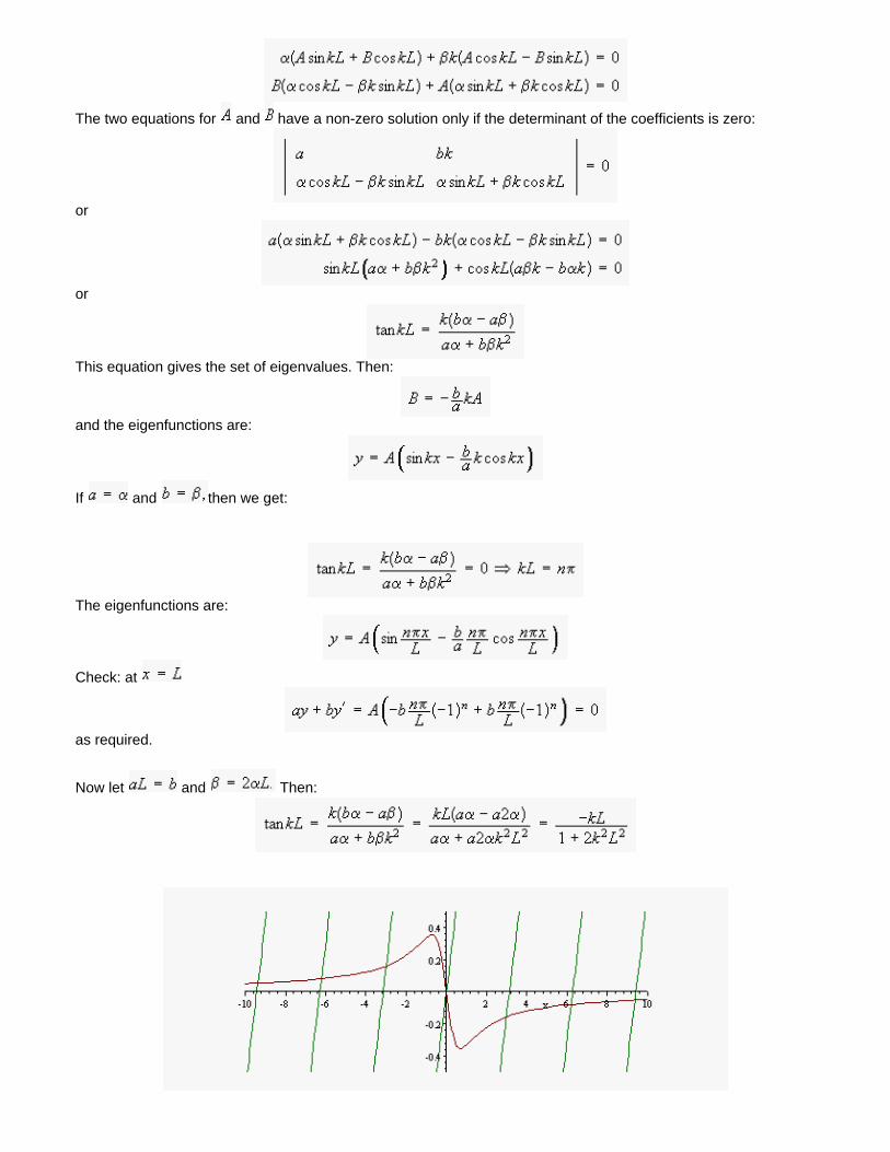
The two equations for and have a non-zero solution only if the determinant of the coefficients is zero:
or
or
This equation gives the set of eigenvalues. Then:
and the eigenfunctions are:
If and then we get:
The eigenfunctions are:
Check: at
as required.
Now let and Then:
, Solutions are: etc.
3. The displacement of a square, vibrating membrane of side satisfies the two-dimensional Helmholtz equation
where , is the frequency and is the speed of waves on the membrane. Suppose the membrane is
fixed at its edges at and Separate variables and solve for the eigenfunctions Show that the system exhibits degeneracy, that is, there is more than one eigenfunction corresponding to a given eigenvalue
In the particular, show that there are two eigenfunctions and that correspond to the eigenvalue
. What symmetry of the physical system causes this degeneracy? (Hints: (a) where are the nodal
lines for the two modes? (b) what happens if one side of the membrane is slightly shorter, equal to ) Any linear combination of the two eigenfunctions is also a solution. Find some of the nodal lines for combinations of
the modes, eg How do these modes reflect the symmetry of the system? Can you find an eigenvalue that has three-fold degeneracy? If so, what do those modes look like?
Separating variables, we have where:
The separated equations are
To satisfy the boundary conditions we need the solution and the eigenvalue Similarly
and thus The eigenfunctions have the form
Thus the two eigenvalues and have the same eigenvalue. This is a reflection of the fact that the system
may be rotated by without change. This rotation changes to Changing the length of one of the
sides destroys the symmtery and removes the degeneracy. The nodal lines for the mode are at
and at Rotation by sends one set of lines to the other. The linear combinations look like:
With we get
With the nodal lines are given by
or
that is
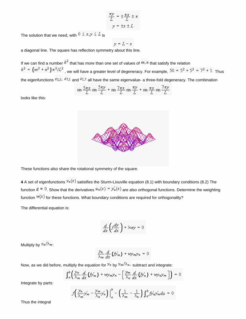
The solution that we need, with is
a diagonal line. The square has reflection symmetry about this line.
If we can find a number that has more than one set of values of that satisfy the relation
, we will have a greater level of degeneracy. For example, Thus
the eigenfunctions and all have the same eigenvalue- a three-fold degeneracy. The combination
looks like this:
These functions also share the rotational symmetry of the square.
4 A set of eigenfunctions satisifies the Sturm-Liouville equation (8.1) with boundary conditions (8.2) The
function . Show that the derivatives are also orthogonal functions. Determine the weighting
function for these functions. What boundary conditions are required for orthogonality?
The differential equation is:
Multiply by :
Now, as we did before, multiply the equation for by subtract and integrate:
Integrate by parts:
Thus the integral
unless provided that:
This will be the case if, for example,
(a) as in the case of Legendre functions.
(b)
(c) and
(e)
etc.
5. Use the recursion relations to show that the derivatives of the Legendre polynomials are orthogonal on
the range (-1,1) with weighting function in agreement with the results of problem 4.
Using the ladder relations, we have
Thus:
Integrating by parts on the right hand side:
and
Thus the right hand side is:
which demonstrates that the are orthogonal with weighting function
6. To obtain Fourier-Legendre series we often need to evaluate integrals of the form:
(a) Start by evaluating and
This integral was evaluated in the text (Example 8.2). We found:
for odd, and zero for even (except .
We do the next integral by parts, using the recursion relation (8.39):
The integrated term is zero, and we can use our first result to do the remaining integrals. The result is zero if is
odd, and for even we get:
.Next:
and
(b) Now working from equation 8.37 we get:
So:
(c) Use these results to ''step down'' until you can use your results from (a) to obtain an explicit expression for
First consider the case We step down using the result above to get:
Let's check this against our previous result for
which checks OK.
Now if we get:
which is zero if is even and for odd we get:
Check against the result for We got zero for odd (i.e. even, as required.)
which checks with the result calculated in part (a).
If Then
7. We have already verified in the text that the formula gives the correct normalization for and Then:
Now evaluate this at All terms except the last are zero, and thus:
and thus
as required.
8. Evaluate the integral
and hence obtain a Fourier-Legendre series for the function
Start with and Then:
Making the change of variable
and so
and
Indeed the result is zero for all odd because in that case the integrand is odd.
Next use the ladder relation:
and integrate by parts. The first term is:
Thus
and using the ladder operator again, we get
In the second term we use the pure recursion relation:
and thus
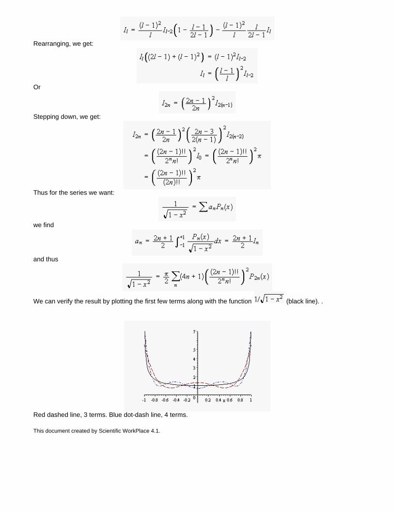
Rearranging, we get:
Or
Stepping down, we get:
Thus for the series we want:
we find
and thus
We can verify the result by plotting the first few terms along with the function (black line). .
Red dashed line, 3 terms. Blue dot-dash line, 4 terms.
This document created by Scientific WorkPlace 4.1.
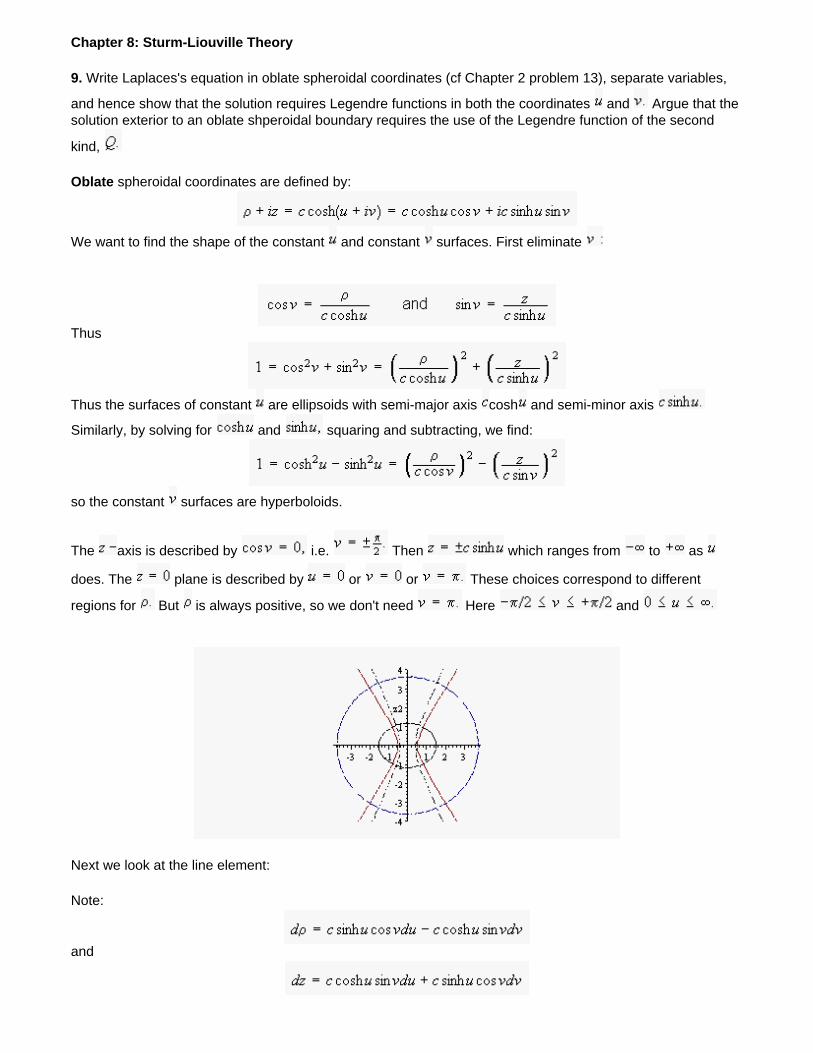
Chapter 8: Sturm-Liouville Theory
9. Write Laplaces's equation in oblate spheroidal coordinates (cf Chapter 2 problem 13), separate variables,
and hence show that the solution requires Legendre functions in both the coordinates and Argue that the solution exterior to an oblate shperoidal boundary requires the use of the Legendre function of the second
kind,
Oblate spheroidal coordinates are defined by:
We want to find the shape of the constant and constant surfaces. First eliminate
Thus
Thus the surfaces of constant are ellipsoids with semi-major axis cosh and semi-minor axis
Similarly, by solving for and squaring and subtracting, we find:
so the constant surfaces are hyperboloids.
The axis is described by i.e. Then which ranges from to as
does. The plane is described by or or These choices correspond to different
regions for But is always positive, so we don't need Here and
Next we look at the line element:
Note:
and
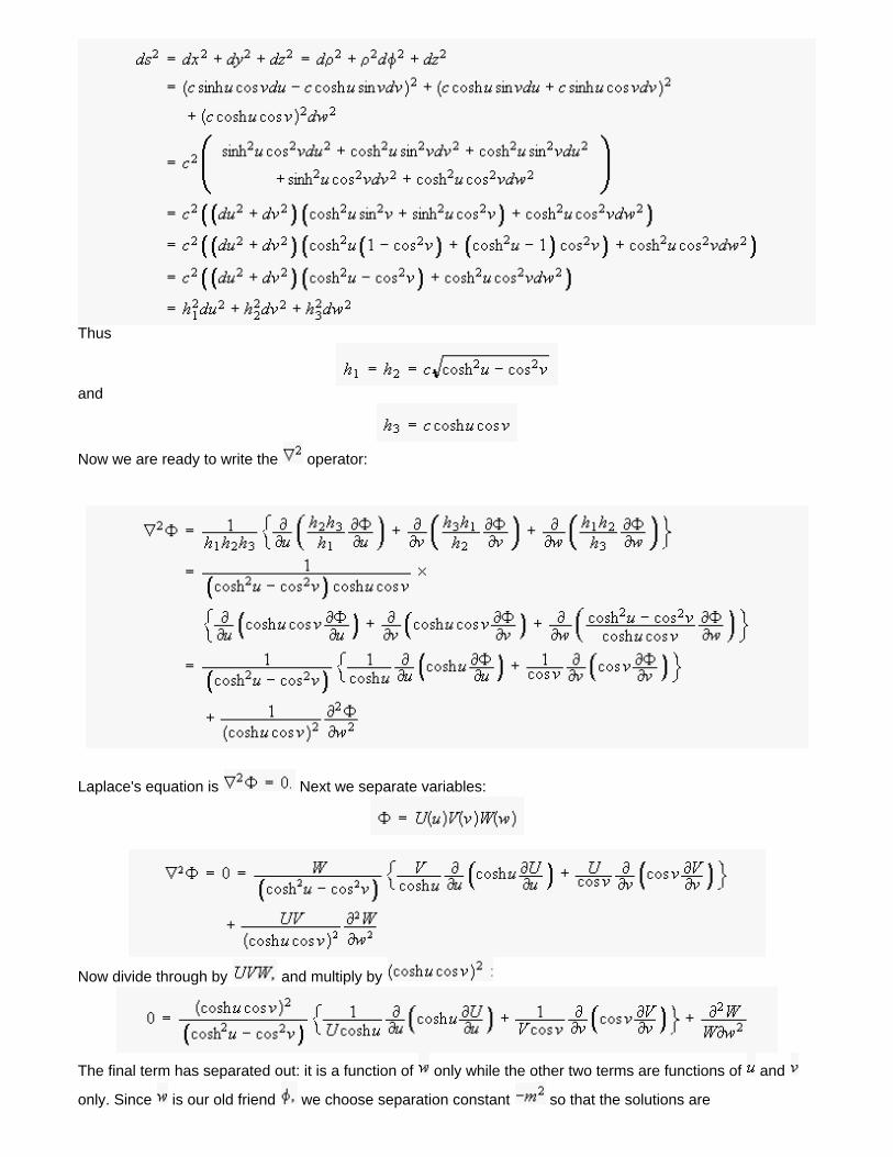
Thus
and
Now we are ready to write the operator:
Laplace's equation is Next we separate variables:
Now divide through by and multiply by
The final term has separated out: it is a function of only while the other two terms are functions of and
only. Since is our old friend we choose separation constant so that the solutions are
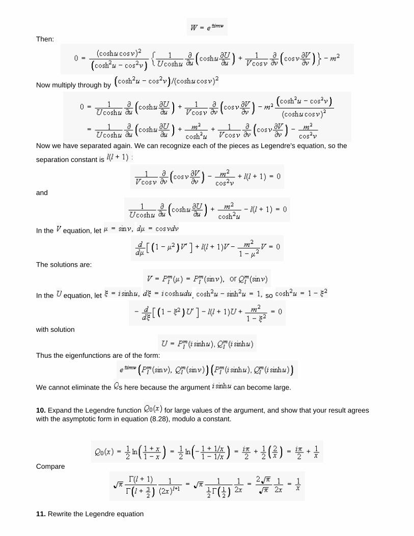
Then:
Now multiply through by
Now we have separated again. We can recognize each of the pieces as Legendre's equation, so the
separation constant is
and
In the equation, let
The solutions are:
In the equation, let , so
with solution
Thus the eigenfunctions are of the form:
We cannot eliminate the s here because the argument can become large.
10. Expand the Legendre function for large values of the argument, and show that your result agrees with the asymptotic form in equation (8.28), modulo a constant.
Compare
11. Rewrite the Legendre equation
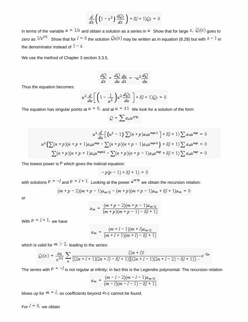
in terms of the variable and obtain a solution as a series in Show that for large goes to
zero as Show that for the solution may be written as in equation (8.28) but with in
the denominator instead of
We use the method of Chapter 3 section 3.3.5.
Thus the equation becomes:
The equation has singular points at and at We look for a solution of the form
The lowest power is which gives the indicial equation:
with solutions and Looking at the power we obtain the recursion relation:
or
With we have
which is valid for leading to the series:
The series with is not regular at infinity; in fact this is the Legendre polynomial. The recursion relation
blows up for so coefficients beyond cannot be found.
For we obtain
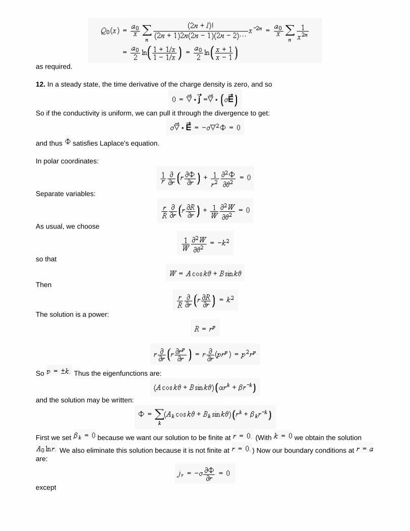
as required.
12. In a steady state, the time derivative of the charge density is zero, and so
So if the conductivity is uniform, we can pull it through the divergence to get:
and thus satisfies Laplace's equation.
In polar coordinates:
Separate variables:
As usual, we choose
so that
Then
The solution is a power:
So Thus the eigenfunctions are:
and the solution may be written:
First we set because we want our solution to be finite at (With we obtain the solution
We also eliminate this solution because it is not finite at ) Now our boundary conditions at are:
except
and
This is a Neumann problem. Inserting the solution for we have
Now we make use of the orthogonality of the trig functions. Multiply both sides by and integrate. Only
the one cosine term with survives the integration:
while for the sine terms we get:
Thus:
and
Then
The first term is:
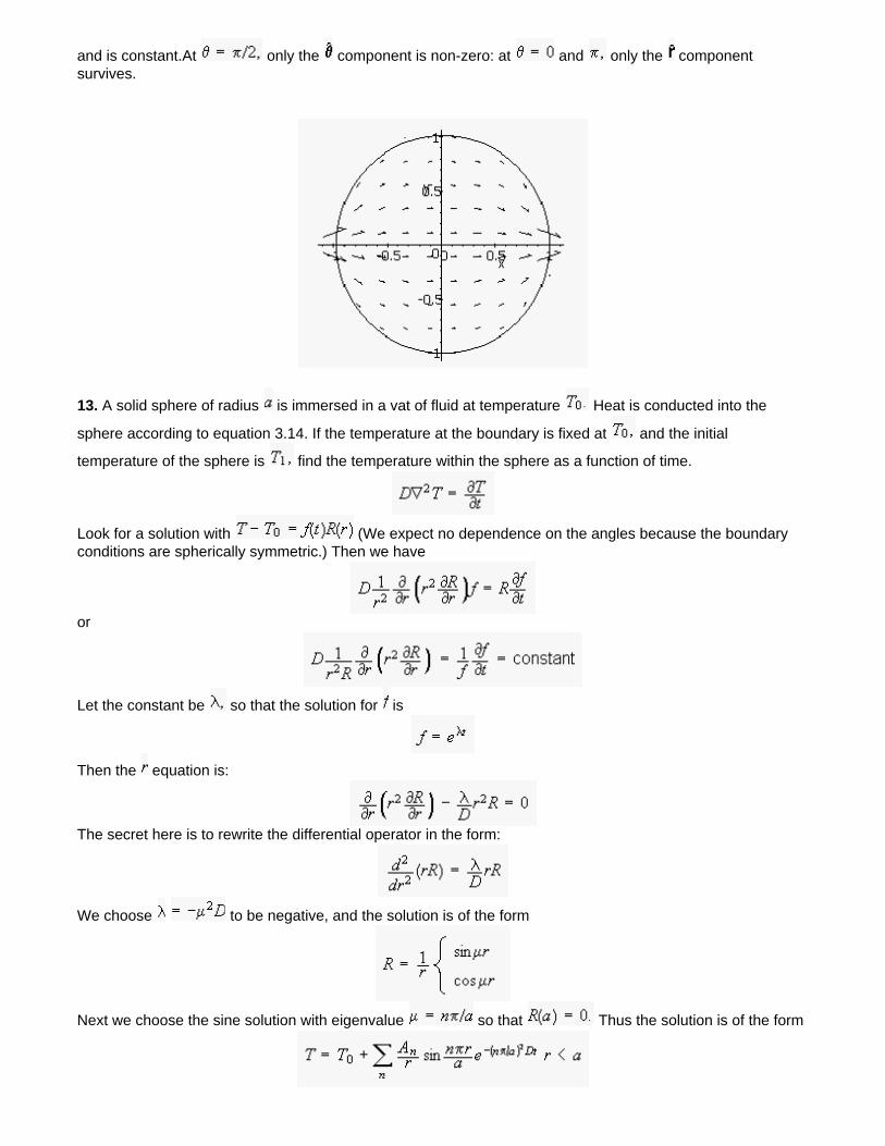
and is constant.At only the component is non-zero: at and only the component survives.
13. A solid sphere of radius is immersed in a vat of fluid at temperature Heat is conducted into the
sphere according to equation 3.14. If the temperature at the boundary is fixed at and the initial
temperature of the sphere is find the temperature within the sphere as a function of time.
Look for a solution with (We expect no dependence on the angles because the boundary conditions are spherically symmetric.) Then we have
or
Let the constant be so that the solution for is
Then the equation is:
The secret here is to rewrite the differential operator in the form:
We choose to be negative, and the solution is of the form
Next we choose the sine solution with eigenvalue so that Thus the solution is of the form
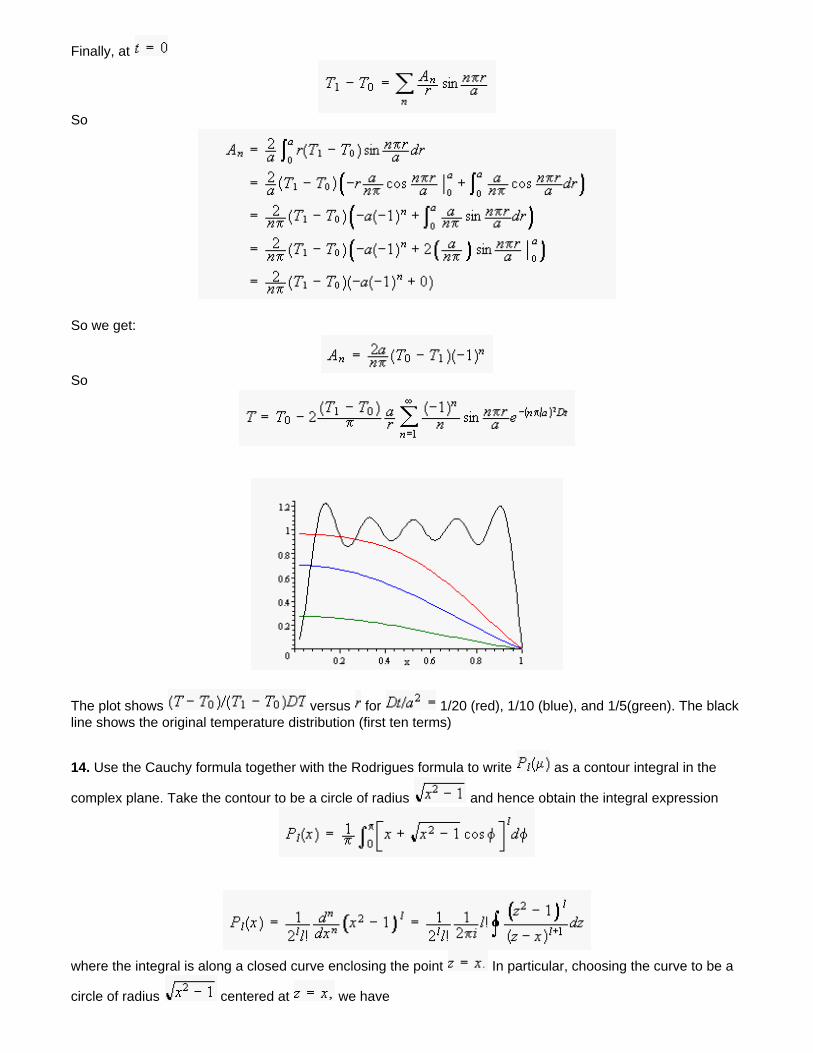
Finally, at
So
So we get:
So
The plot shows versus for 1/20 (red), 1/10 (blue), and 1/5(green). The black line shows the original temperature distribution (first ten terms)
14. Use the Cauchy formula together with the Rodrigues formula to write as a contour integral in the
complex plane. Take the contour to be a circle of radius and hence obtain the integral expression
where the integral is along a closed curve enclosing the point In particular, choosing the curve to be a
circle of radius centered at we have
This document created by Scientific WorkPlace 4.1.
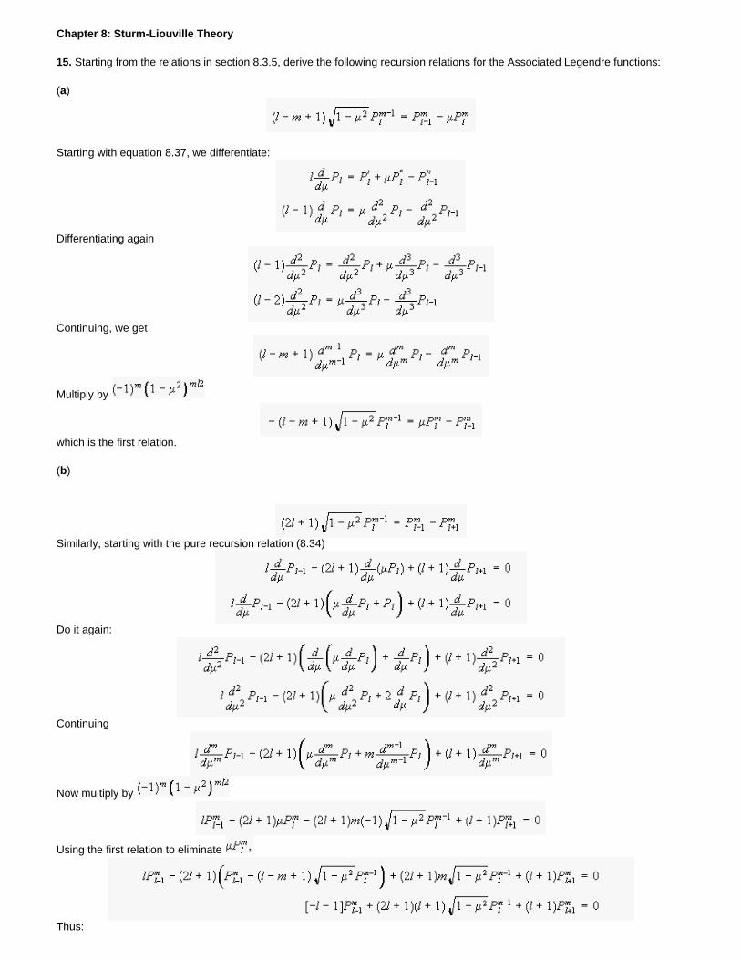
Chapter 8: Sturm-Liouville Theory
15. Starting from the relations in section 8.3.5, derive the following recursion relations for the Associated Legendre functions:
(a)
Starting with equation 8.37, we differentiate:
Differentiating again
Continuing, we get
Multiply by
which is the first relation.
(b)
Similarly, starting with the pure recursion relation (8.34)
Do it again:
Continuing
Now multiply by
Using the first relation to eliminate
Thus:
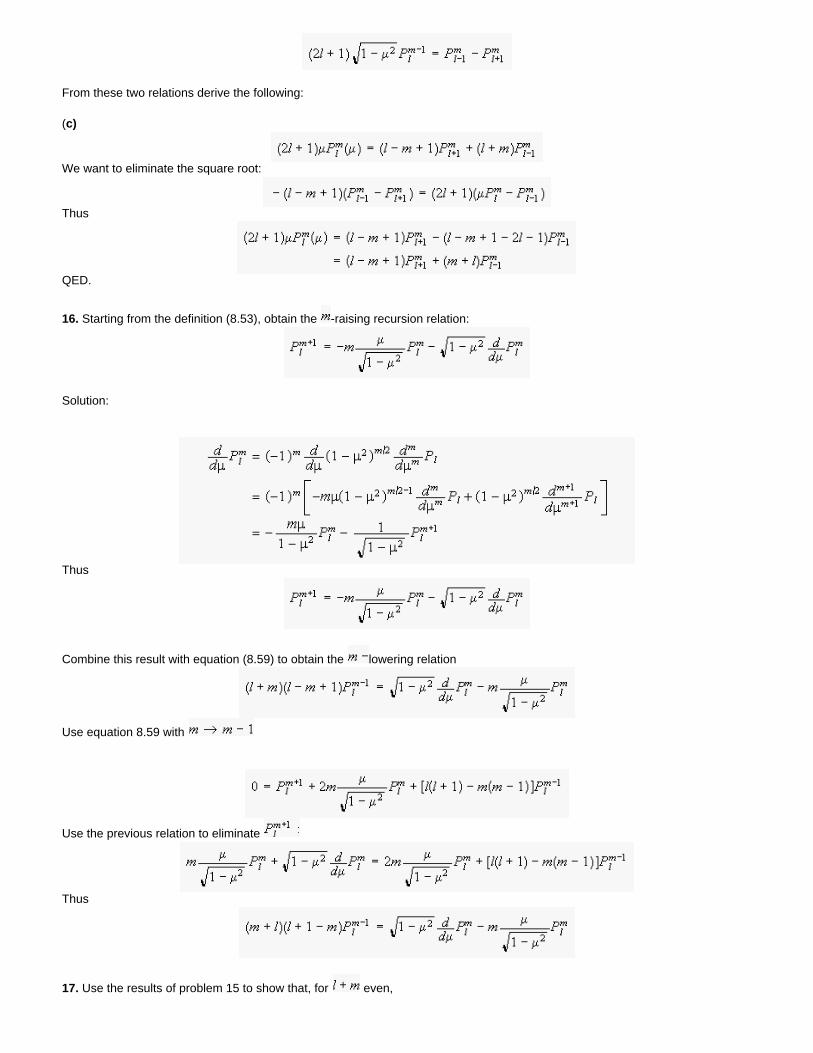
From these two relations derive the following:
(c)
We want to eliminate the square root:
Thus
QED.
16. Starting from the definition (8.53), obtain the -raising recursion relation:
Solution:
Thus
Combine this result with equation (8.59) to obtain the lowering relation
Use equation 8.59 with
Use the previous relation to eliminate
Thus
17. Use the results of problem 15 to show that, for even,
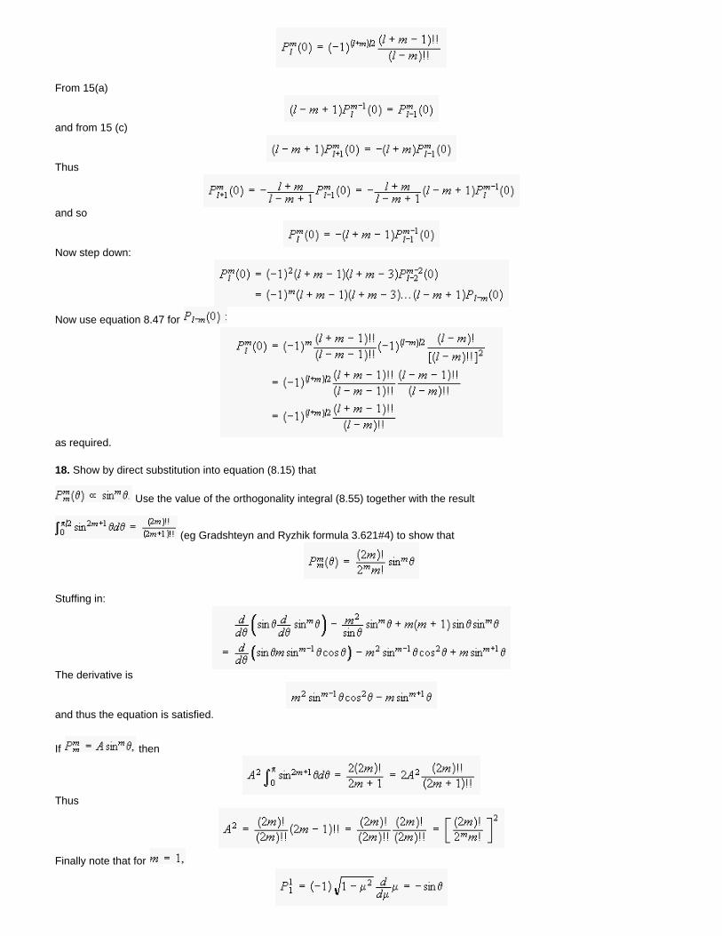
From 15(a)
and from 15 (c)
Thus
and so
Now step down:
Now use equation 8.47 for
as required.
18. Show by direct substitution into equation (8.15) that
Use the value of the orthogonality integral (8.55) together with the result
(eg Gradshteyn and Ryzhik formula 3.621#4) to show that
Stuffing in:
The derivative is
and thus the equation is satisfied.
If then
Thus
Finally note that for
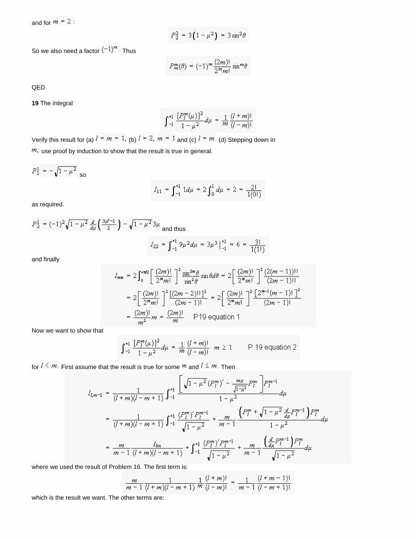
and for
So we also need a factor Thus
QED
19 The integral
Verify this result for (a) (b) and (c) (d) Stepping down in
use proof by induction to show that the result is true in general.
so
as required.
and thus
and finally
Now we want to show that
for First assume that the result is true for some and Then
where we used the result of Problem 16. The first term is:
which is the result we want. The other terms are:
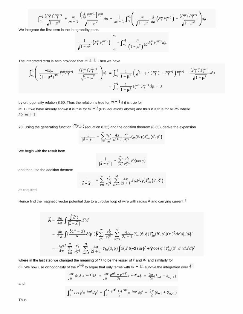
We integrate the first term in the integrandby parts:
The integrated term is zero provided that Then we have
by orthogonality relation 8.50. Thus the relation is true for if it is true for
But we have already shown it is true for (P19 equation1 above) and thus it is true for all where
20. Using the generating function (equation 8.32) and the addition theorem (8.65), derive the expansion
We begin with the result from
and then use the addition theorem
as required.
Hence find the magnetic vector potential due to a circular loop of wire with radius and carrying current
where in the last step we changed the meaning of to be the lesser of and and similarly for
We now use orthogonality of the to argue that only terms with survive the integration over
and
Thus
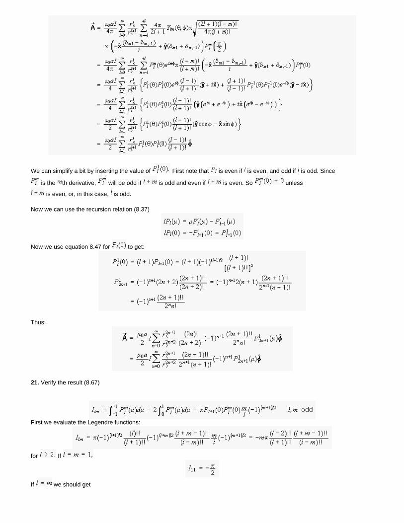
We can simplify a bit by inserting the value of First note that is even if is even, and odd if is odd. Since
is the th derivative, will be odd if is odd and even if is even. So unless
is even, or, in this case, is odd.
Now we can use the recursion relation (8.37)
Now we use equation 8.47 for to get:
Thus:
21. Verify the result (8.67)
First we evaluate the Legendre functions:
for If
If we should get
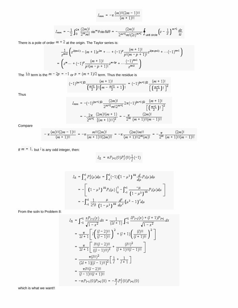
There is a pole of order at the origin. The Taylor series is:
The term is the or term. Thus the residue is
Thus
Compare
If but is any odd integer, then:
From the soln to Problem 8:
which is what we want!!
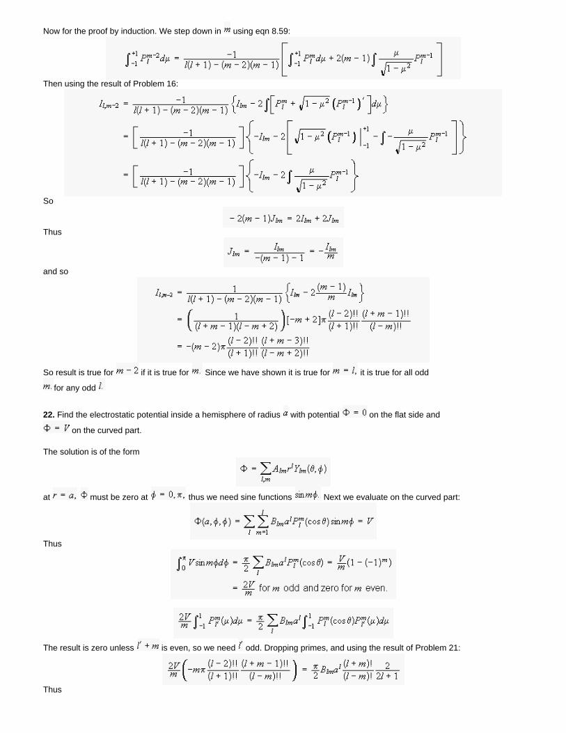
Now for the proof by induction. We step down in using eqn 8.59:
Then using the result of Problem 16:
So
Thus
and so
So result is true for if it is true for Since we have shown it is true for it is true for all odd
for any odd
22. Find the electrostatic potential inside a hemisphere of radius with potential on the flat side and
on the curved part.
The solution is of the form
at must be zero at thus we need sine functions Next we evaluate on the curved part:
Thus
The result is zero unless is even, so we need odd. Dropping primes, and using the result of Problem 21:
Thus
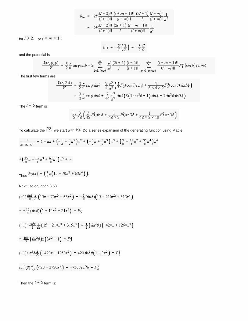
for For
and the potential is
The first few terms are:
The term is
To calculate the we start with Do a series expansion of the generating function using Maple:
Thus
Next use equation 8.53.
Then the term is:
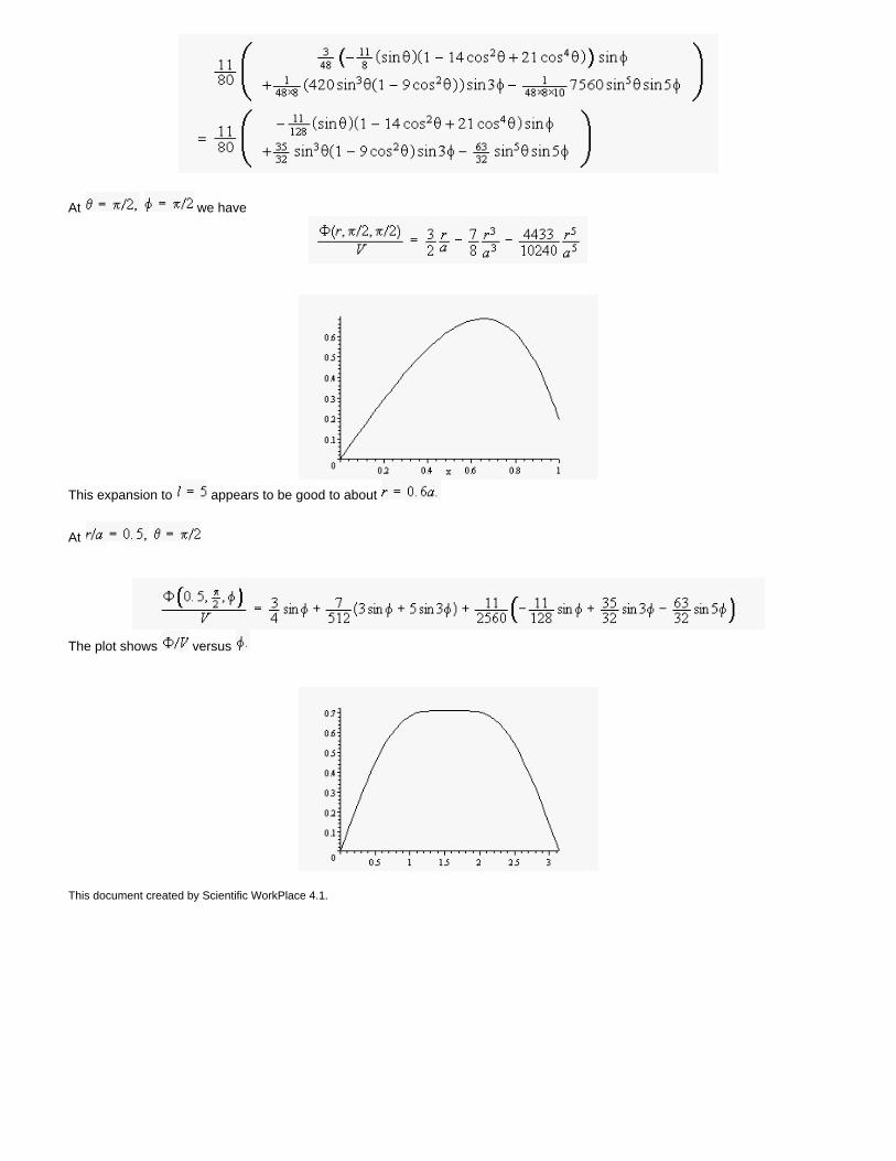
At we have
This expansion to appears to be good to about
At
The plot shows versus
This document created by Scientific WorkPlace 4.1.
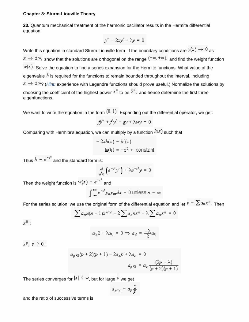
Chapter 8: Sturm-Liouville Theory
23. Quantum mechanical treatment of the harmonic oscillator results in the Hermite differential equation
Write this equation in standard Sturm-Liouville form. If the boundary conditions are as
show that the solutions are orthogonal on the range and find the weight function
Solve the equation to find a series expansion for the Hermite functions. What value of the
eigenvalue is required for the functions to remain bounded throughout the interval, including
? (Hint: experience with Legendre functions should prove useful.) Normalize the solutions by
choosing the coefficient of the highest power to be and hence determine the first three eigenfunctions.
We want to write the equation in the form Expanding out the differential operator, we get:
Comparing with Hermite's equation, we can multiply by a function such that
Thus and the standard form is:
Then the weight function is and
For the series solution, we use the original form of the differential equation and let Then
The series converges for , but for large we get
and the ratio of successive terms is
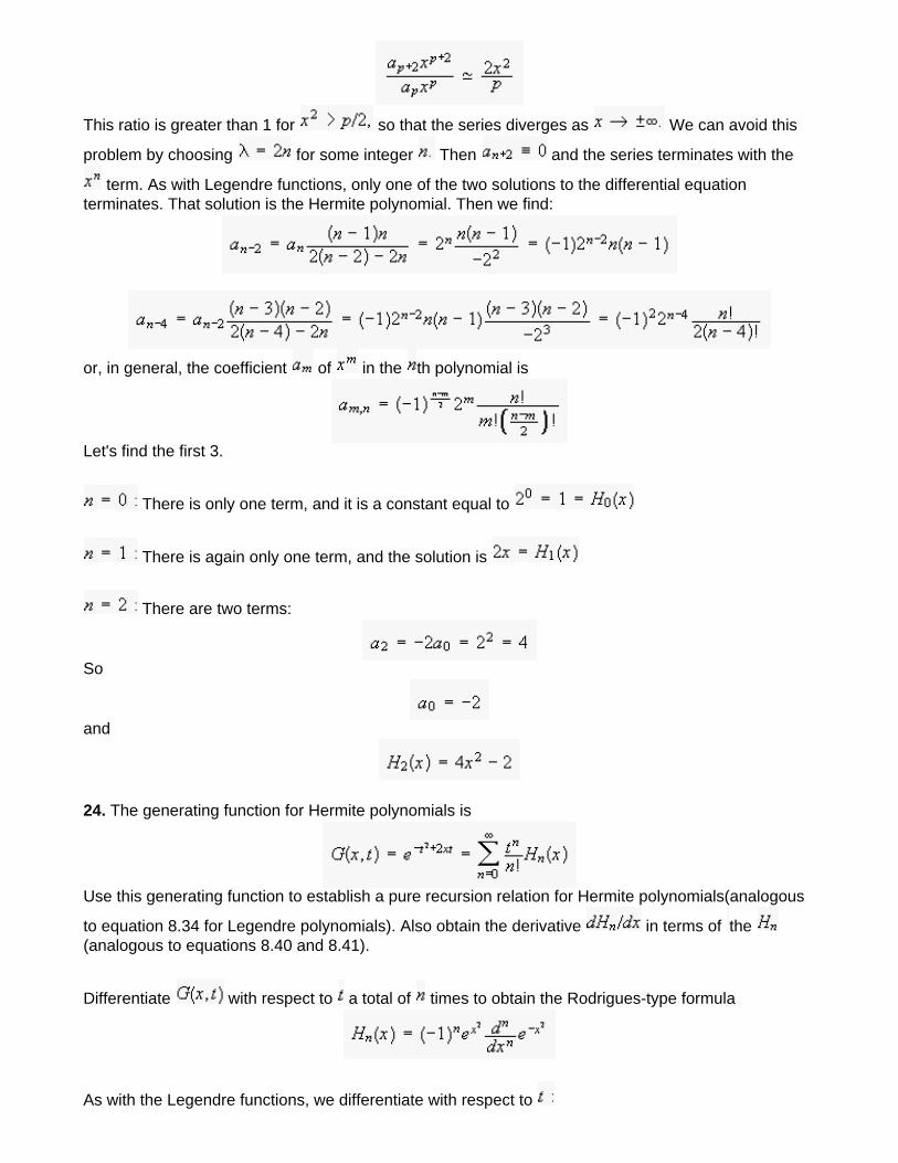
This ratio is greater than 1 for so that the series diverges as We can avoid this
problem by choosing for some integer Then and the series terminates with the
term. As with Legendre functions, only one of the two solutions to the differential equation terminates. That solution is the Hermite polynomial. Then we find:
or, in general, the coefficient of in the th polynomial is
Let's find the first 3.
There is only one term, and it is a constant equal to
There is again only one term, and the solution is
There are two terms:
So
and
24. The generating function for Hermite polynomials is
Use this generating function to establish a pure recursion relation for Hermite polynomials(analogous
to equation 8.34 for Legendre polynomials). Also obtain the derivative in terms of the (analogous to equations 8.40 and 8.41).
Differentiate with respect to a total of times to obtain the Rodrigues-type formula
As with the Legendre functions, we differentiate with respect to
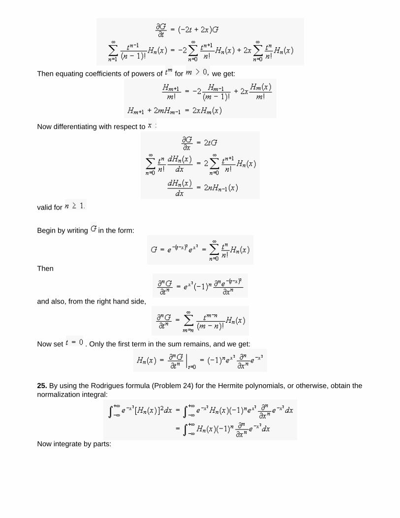
Then equating coefficients of powers of for we get:
Now differentiating with respect to
valid for
Begin by writing in the form:
Then
and also, from the right hand side,
Now set . Only the first term in the sum remains, and we get:
25. By using the Rodrigues formula (Problem 24) for the Hermite polynomials, or otherwise, obtain the normalization integral:
Now integrate by parts:
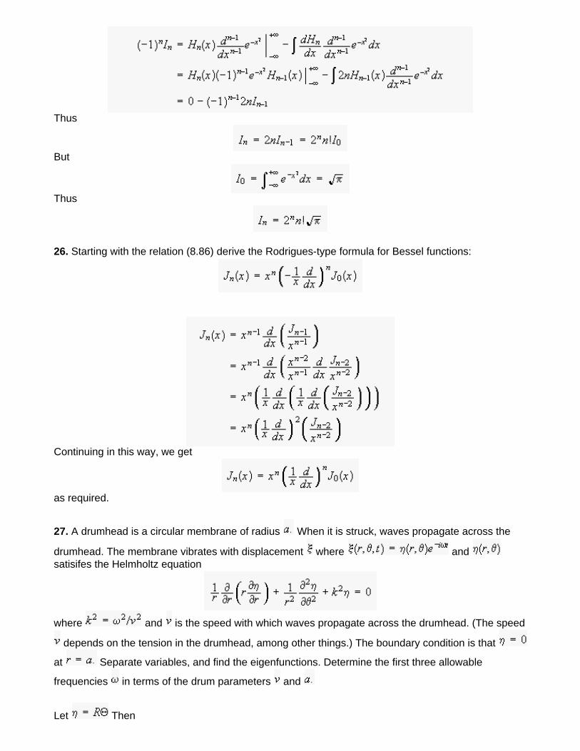
Thus
But
Thus
26. Starting with the relation (8.86) derive the Rodrigues-type formula for Bessel functions:
Continuing in this way, we get
as required.
27. A drumhead is a circular membrane of radius When it is struck, waves propagate across the
drumhead. The membrane vibrates with displacement where and satisifes the Helmholtz equation
where and is the speed with which waves propagate across the drumhead. (The speed
depends on the tension in the drumhead, among other things.) The boundary condition is that
at Separate variables, and find the eigenfunctions. Determine the first three allowable
frequencies in terms of the drum parameters and
Let Then
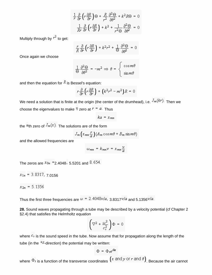
Multiply through by to get:
Once again we choose
and then the equation for is Bessel's equation:
We need a solution that is finite at the origin (the center of the drumhead), i.e. Then we
choose the eigenvalues to make zero at Thus
the th zero of The solutions are of the form
and the allowed frequencies are
The zeros are 2.4048 5.5201 and
7.0156
Thus the first three frequencies are 3.8317 and 5.1356
28. Sound waves propagating through a tube may be described by a velocity potential (cf Chapter 2 §2.4) that satisfies the Helmholtz equation
where is the sound speed in the tube. Now assume that for propagation along the length of the
tube (in the -direction) the potential may be written:
where is a function of the transverse coordinates . Because the air cannot
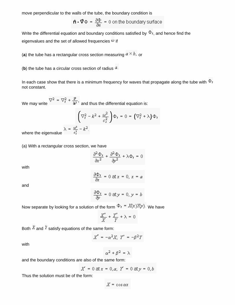
move perpendicular to the walls of the tube, the boundary condition is
Write the differential equation and boundary conditions satisfied by , and hence find the
eigenvalues and the set of allowed frequencies if
(a) the tube has a rectangular cross section measuring or
(b) the tube has a circular cross section of radius
In each case show that there is a minimum frequency for waves that propagate along the tube with not constant.
We may write and thus the differential equation is:
where the eigenvalue
(a) With a rectangular cross section, we have
with
and
Now separate by looking for a solution of the form We have
Both and satisfy equations of the same form:
with
and the boundary conditions are also of the same form:
Thus the solution must be of the form:
so that at Then we choose the eigenvalue so that i.e.
Doing the same thing for we find that the eigenfunctions are of the form:
and the eigenvalues are
Thus the allowed frequencies are given by:
The solution with corresponds to a constant value of With constant, the air velocity is identically zero, and so there is no wave. Otherwise,
The minimum frequency occurs for and either or . (For lesser frequencies
becomes imaginary and the wave does not propagate.) If the larger dimension of the tube is then the minimum frequency is:
(b) With the differential equation is
which separates to give
and
which is Bessel's equation, with solution
The boundary condition at requires that we choose to be one one of the roots
of Then the eigenvalue Then the frequency is
With and is a constant and there is no wave. Otherwise, the smallest value of
is giving a cut-off frequency of
Compare this with the rectangular guide: the closest equivalent dimension to the radius is one half the
dimension and the cutoff is
which is comparable to that for the circular guide.
Writing or in the case of circular or square guides, we have
and
repectively.
29. If is the th zero of show that the Bessel functions satisfy the orthogonality relation:
We start with the general orthogonality relation (equation 8.6)
Integrating by parts, the first term on the right hand side is:
Subtracting the second term, the integrals cancel. Taking another zero of , the integrated terms are both zero, and so we have
To obtain the value of the integral if we differentiate with respect to
On the right hand side, we make use of the differential equation to get:
Now let The first term on the left goes to zero, and we have:
The contribution from the lower limit is zero for since in that case, and is zero for
because then the factor multiplying is Thus
which is the required result.
30. Use the generating function (8.93) to show that
We start with
Let Then
Now let
Now subtract the two results:
For the even terms:
while for the odd terms
and
Then since
for odd we may combine the positive and negative terms to get:
(b)
This time we set Then
The odd terms in the sum are zero, leaving
as required.
This document created by Scientific WorkPlace 4.1.
Chapter 8: Sturm-Liouville Theory
31. Show that
Start with:
and
Multiply these results together:
Now multiply both sides by and integrate over the range to 2
By the orthogonality of the exponential functions, only the term with
survives on the left, and the terms with on the right:
as required.
Now let and to get:
32. Show that
We use the technique from Appendix VIII.
Since the series for starts with the integrated term is zero at provided that
and the integrand vanishes, so, using the large argument expansion of the Bessel functions, we are left with:
The first term as because of the factor Thus we are left with:
and thus
Then as we get:
This agrees with GR 6.538#2 with
Note that the Bessel equation may be considered as an eigenvalue problem with eigenvalue
with and the weighting function Our proof shows that
if is not equal to and
is an even integer. Thus the even order Bessel functions or odd order Bessel functions satisfy a second
orthogonality relation. This is somewhat analogous to the orthogonality of sines or cosines on the half range
33. At time the surface of the water in a pond has the form
and
By taking the Fourier transform of the wave equation with two spatial dimensions, find the displacement
at later times.
Thus
and thus
where (a)
and
Thus
We may make use of the integral expression (8.92) for the Bessel function to obtain:
Now multiply both sides by and integrate
Thus
The initial disturbance oscillates in time.
34. Evaluate the integral
Now we let , and use the methods of Chapter 2 §2.7.2:
The integrand has poles at (for and
Of these, the poles at (order and at are inside the circle.
(The plot is a graph of versus x. All values are between and 0. )
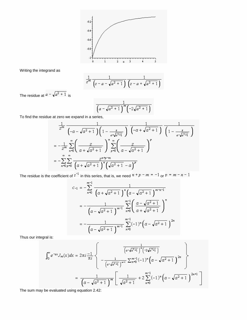
Writing the integrand as
The residue at is
To find the residue at zero we expand in a series,
The residue is the coefficient of in this series, that is, we need or
Thus our integral is:
The sum may be evaluated using equation 2.42:
Thus
For we have the nice result
35.
The result is
if and
if
36. Show that the first zero (other than zero) of the Bessel function is an increasing function of
that is
and so on.
First note that each Bessel function is positive for sufficiently small values of as indicated by the small argument
expansion (8.80). Similarly, for the derivative is also positive for sufficiently small
. The function increases from zero, then decreases to the first zero. Thus the first zero occurs at where
is negative. Now from relations 8.89 and 8.90:
So
Evaluate at to get:
which is therefore positive, and also
is negative. If is negative then for
QED
We still need to show that We know that and therefore Since by
assumption, must be the first minimum of . Furthermore,
and evaluating at
and is therefore negative. These results show that
37. A pendulum has steadily increasing length
Show that the equation that describes small oscillations of this pendulum is:
Change variables to and
and hence show that the general solution may be expressed in terms of Bessel functions. Find the solution if the
pendulum is released from rest at an angle at (
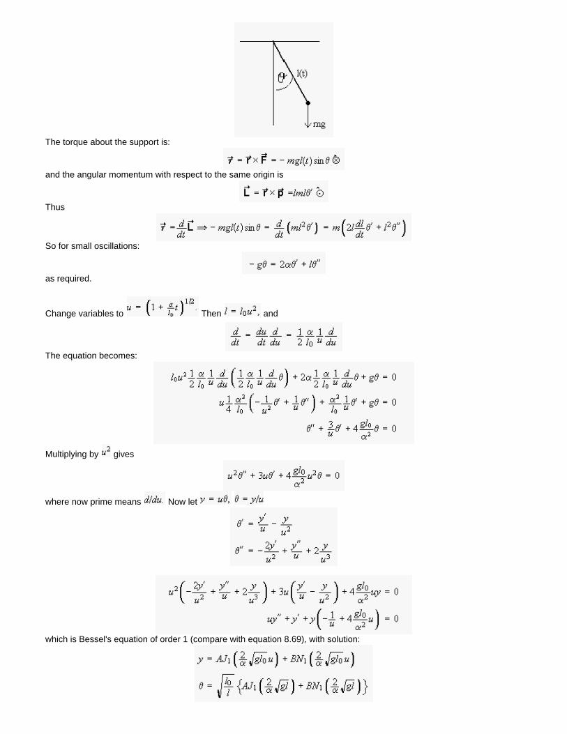
The torque about the support is:
and the angular momentum with respect to the same origin is
Thus
So for small oscillations:
as required.
Change variables to Then and
The equation becomes:
Multiplying by gives
where now prime means Now let
which is Bessel's equation of order 1 (compare with equation 8.69), with solution:
Here we must include in the solution because the argument is never zero. If the pendulum starts from rest when
then
and
So
and thus
The denominator is the Wronskian of the two solutions, and equals:
Using the large arument form of the Bessels, we can evaluate the constant:
Thus
and the solution for is
Check the dimensions: is a length, and so
as is required. The plot shows with and the dimensionless time variable
We used the recursion relation 8.90 to evaluate the derivatives: and similarly for
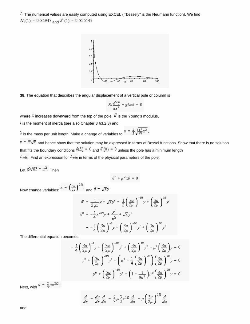
The numerical values are easily computed using EXCEL (``bessely'' is the Neumann function). We find
and
38. The equation that describes the angular displacement of a vertical pole or column is
where increases downward from the top of the pole, is the Young's modulus,
is the moment of inertia (see also Chapter 3 §3.2.3) and
is the mass per unit length. Make a change of variables to
and hence show that the solution may be expressed in terms of Bessel functions. Show that there is no solution
that fits the boundary conditions and unless the pole has a minimum length
Find an expression for in terms of the physical parameters of the pole.
Let Then
Now change variables: and
The differential equation becomes:
Next, with
and
Thus
This is Bessel's equation of order 1/3, so the solution is:
or, in the original variables:
Then
Using the series 8.73 with
and the derivatives are:
Thus
Thus the boundary condition is satisfied if we choose Then:
and so Then to satisfy the second condition, we must have
Thus must be one of the zeroes of Thus
can take on only a specific set of values, and in particular there is a smallest value corresponding to the first zero of
That value is:
or
39. Establish the addition theorem for Bessel functions.
We start by expanding the function where and are vectors in the
plane,. in the complete orthogonal set of functions :
By symmetry in we have
Now let The only non-zero Bessel function is so
From the result of problem 34 in the limit we conclude that Thus
Since this result is valid for any value of we conclude that
Note also that this expression gives correct results in the limit (Problem 31) and in the limit
40. Starting from the definitions 8.100, 8.76 and 8.78, show that::
where is not an integer.
as required. Also
This document created by Scientific WorkPlace 4.1.
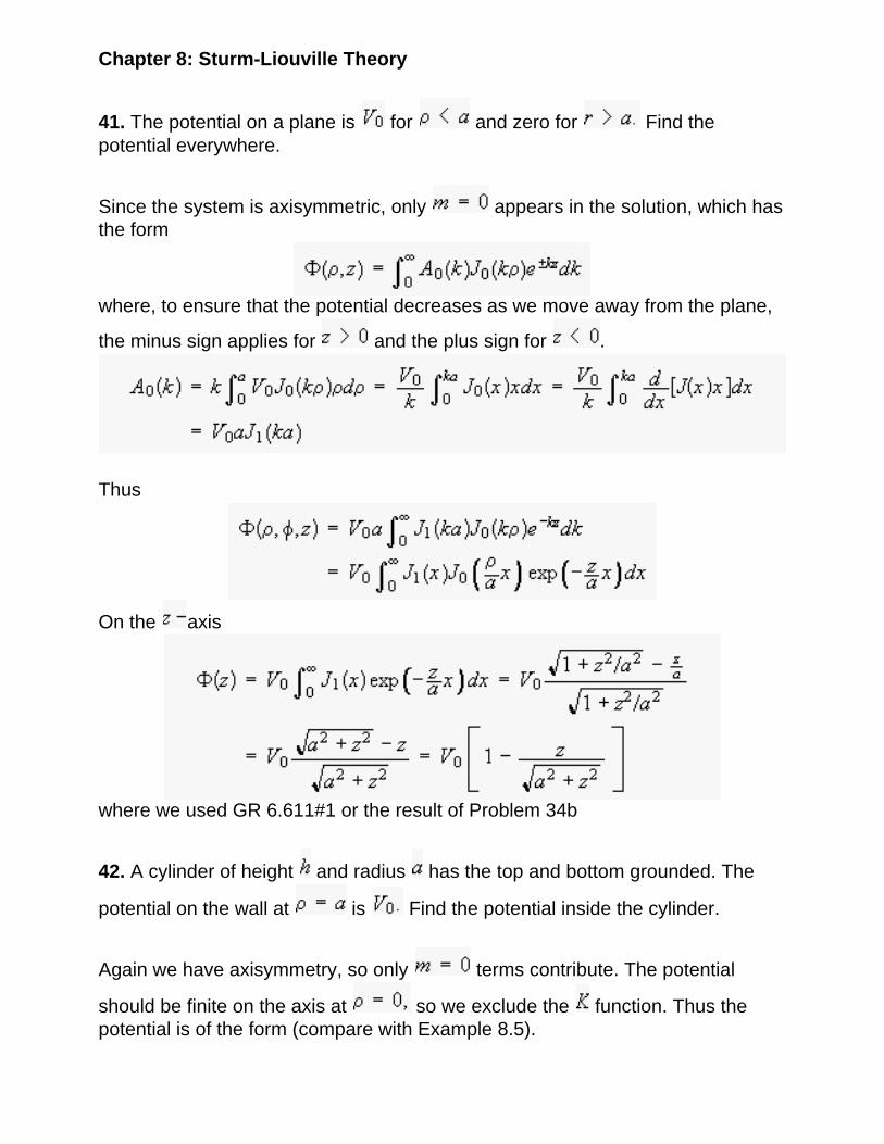
Chapter 8: Sturm-Liouville Theory
41. The potential on a plane is for and zero for Find the potential everywhere.
Since the system is axisymmetric, only appears in the solution, which has the form
where, to ensure that the potential decreases as we move away from the plane,
the minus sign applies for and the plus sign for .
Thus
On the axis
where we used GR 6.611#1 or the result of Problem 34b
42. A cylinder of height and radius has the top and bottom grounded. The
potential on the wall at is Find the potential inside the cylinder.
Again we have axisymmetry, so only terms contribute. The potential
should be finite on the axis at so we exclude the function. Thus the potential is of the form (compare with Example 8.5).
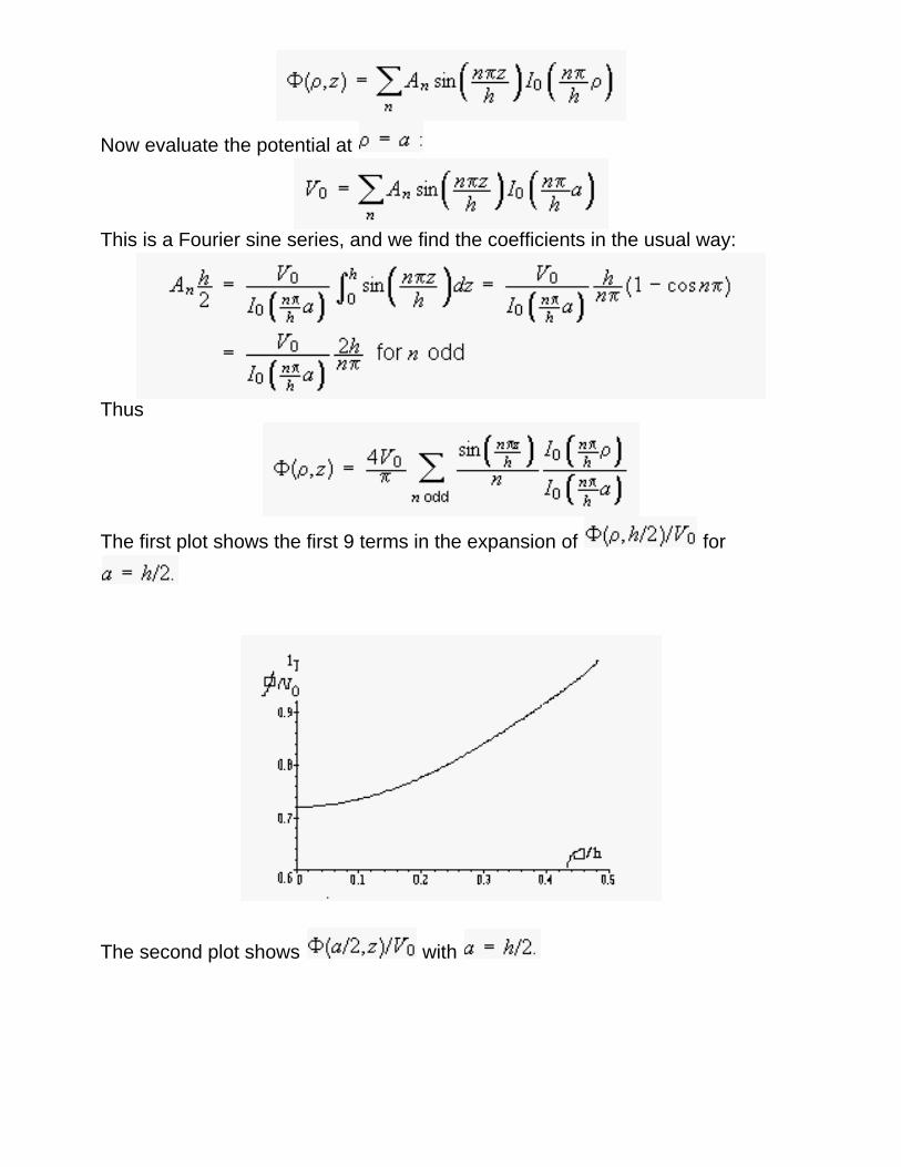
Now evaluate the potential at
This is a Fourier sine series, and we find the coefficients in the usual way:
Thus
The first plot shows the first 9 terms in the expansion of for
The second plot shows with
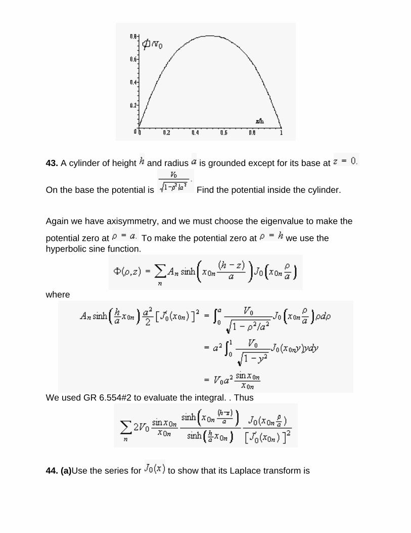
43. A cylinder of height and radius is grounded except for its base at
On the base the potential is Find the potential inside the cylinder.
Again we have axisymmetry, and we must choose the eigenvalue to make the
potential zero at To make the potential zero at we use the hyperbolic sine function.
where
We used GR 6.554#2 to evaluate the integral. . Thus
44. (a)Use the series for to show that its Laplace transform is
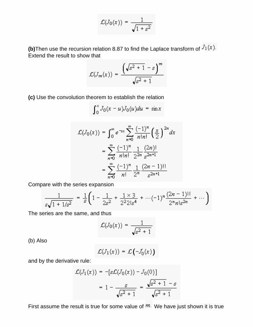
(b)Then use the recursion relation 8.87 to find the Laplace transform of Extend the result to show that
(c) Use the convolution theorem to establish the relation
Compare with the series expansion
The series are the same, and thus
(b) Also
and by the derivative rule:
First assume the result is true for some value of We have just shown it is true
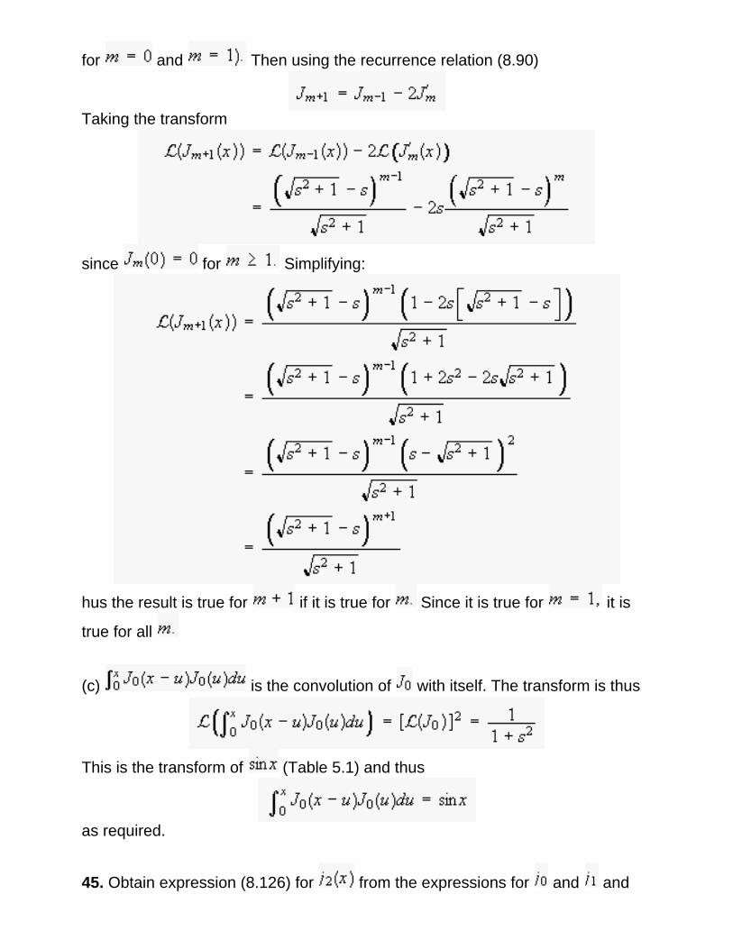
for and Then using the recurrence relation (8.90)
Taking the transform
since for Simplifying:
hus the result is true for if it is true for Since it is true for it is
true for all
(c) is the convolution of with itself. The transform is thus
This is the transform of (Table 5.1) and thus
as required.
45. Obtain expression (8.126) for from the expressions for and and
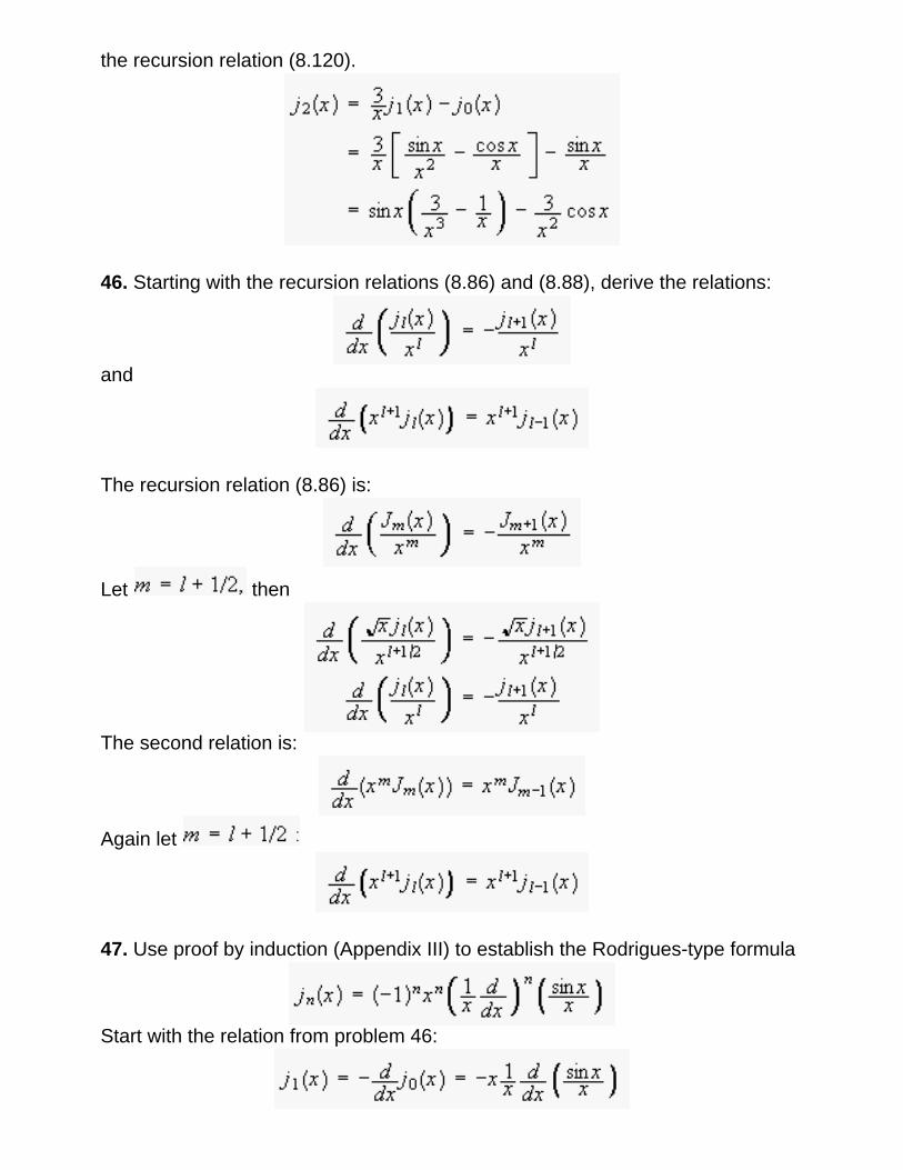
the recursion relation (8.120).
46. Starting with the recursion relations (8.86) and (8.88), derive the relations:
and
The recursion relation (8.86) is:
Let then
The second relation is:
Again let
47. Use proof by induction (Appendix III) to establish the Rodrigues-type formula
Start with the relation from problem 46:
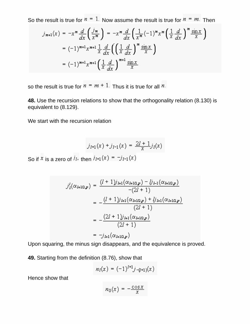
So the result is true for Now assume the result is true for Then
so the result is true for Thus it is true for all
48. Use the recursion relations to show that the orthogonality relation (8.130) is equivalent to (8.129).
We start with the recursion relation
So if is a zero of then
Upon squaring, the minus sign disappears, and the equivalence is proved.
49. Starting from the definition (8.76), show that
Hence show that
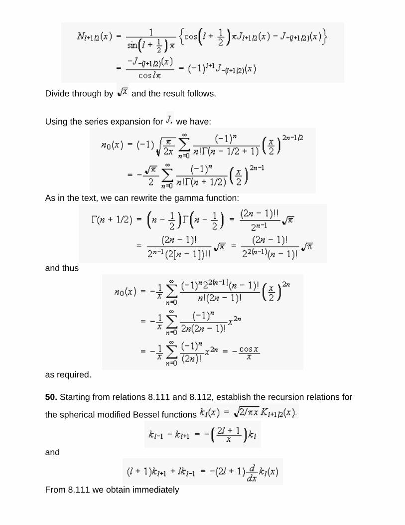
Divide through by and the result follows.
Using the series expansion for we have:
As in the text, we can rewrite the gamma function:
and thus
as required.
50. Starting from relations 8.111 and 8.112, establish the recursion relations for
the spherical modified Bessel functions
and
From 8.111 we obtain immediately
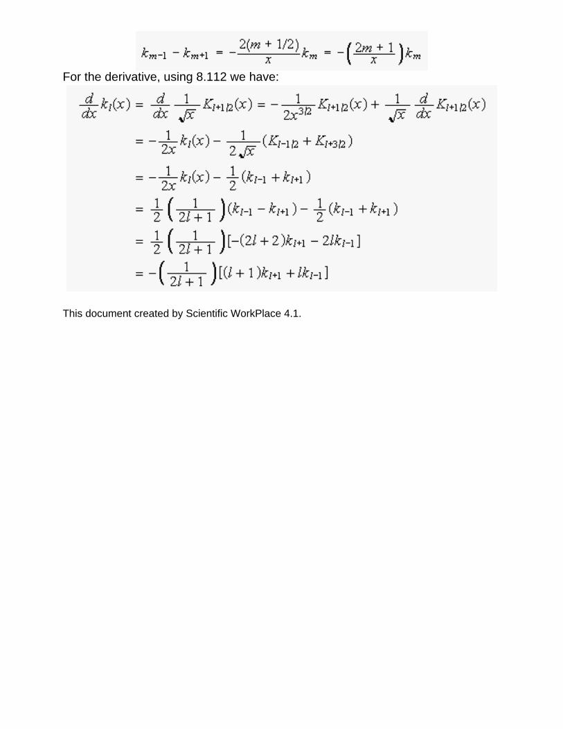
For the derivative, using 8.112 we have:
This document created by Scientific WorkPlace 4.1.
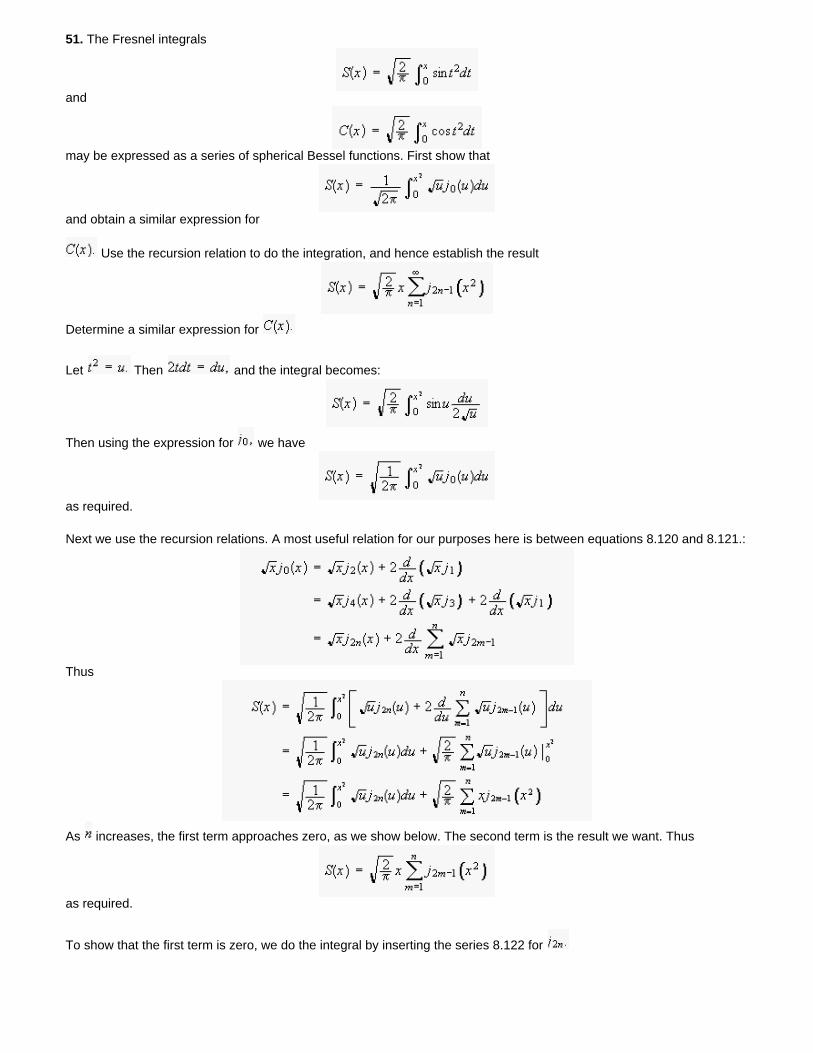
51. The Fresnel integrals
and
may be expressed as a series of spherical Bessel functions. First show that
and obtain a similar expression for
Use the recursion relation to do the integration, and hence establish the result
Determine a similar expression for
Let Then and the integral becomes:
Then using the expression for we have
as required.
Next we use the recursion relations. A most useful relation for our purposes here is between equations 8.120 and 8.121.:
Thus
As increases, the first term approaches zero, as we show below. The second term is the result we want. Thus
as required.
To show that the first term is zero, we do the integral by inserting the series 8.122 for
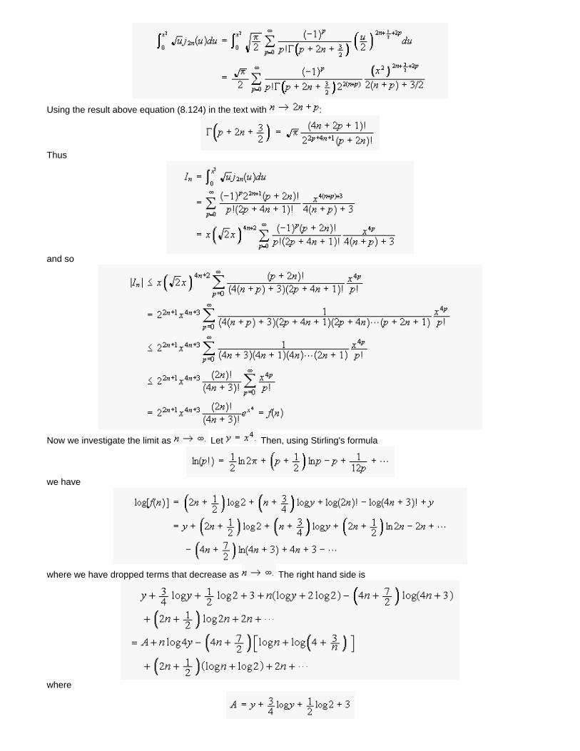
Using the result above equation (8.124) in the text with :
Thus
and so
Now we investigate the limit as Let Then, using Stirling's formula
we have
where we have dropped terms that decrease as The right hand side is
where
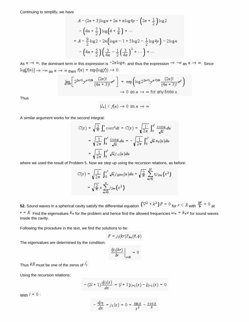
Continuing to simplify, we have
As the dominant term in this expression is and thus the expression as Since
as then
Thus
A similar argument works for the second integral:
where we used the result of Problem 5. Now we step up using the recursion relations, as before:
52. Sound waves in a spherical cavity satisfy the differential equation for with at
Find the eigenvalues for the problem and hence find the allowed frequencies for sound waves inside the cavity.
Following the procedure in the text, we find the solutions to be:
The eigenvalues are determined by the condition:
Thus must be one of the zeros of
Using the recursion relations:
With
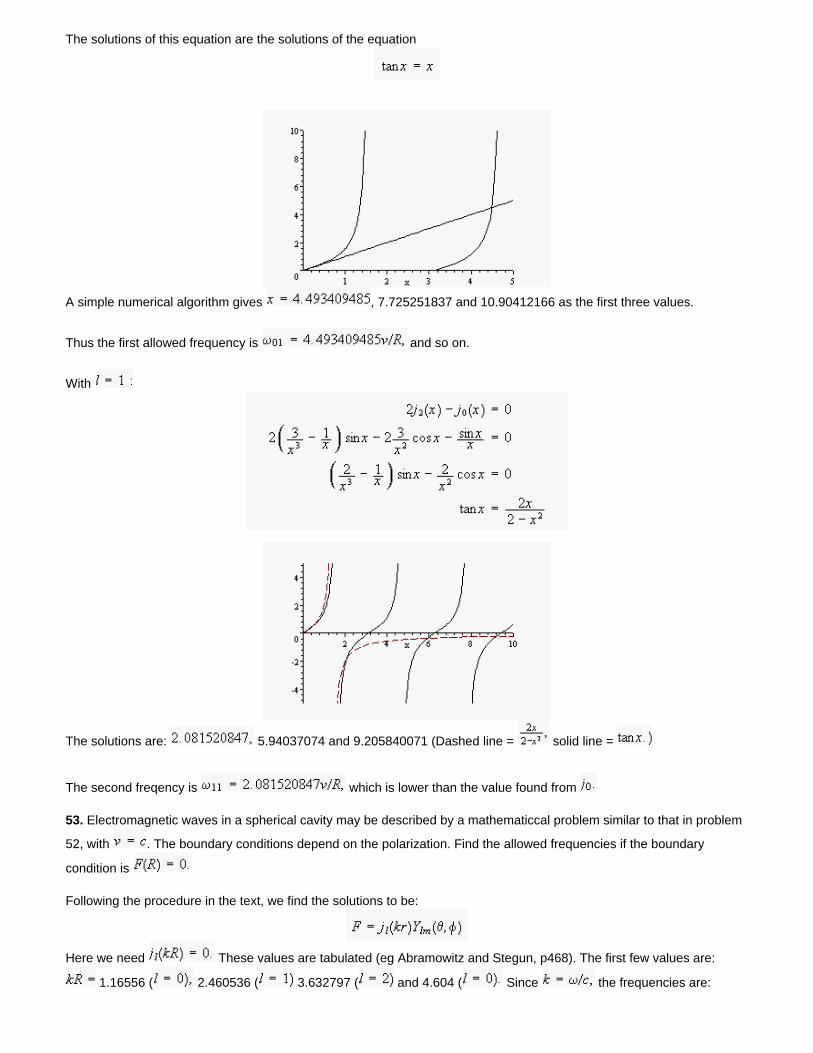
The solutions of this equation are the solutions of the equation
A simple numerical algorithm gives , 7.725251837 and 10.90412166 as the first three values.
Thus the first allowed frequency is and so on.
With
The solutions are: 5.94037074 and 9.205840071 (Dashed line = solid line =
The second freqency is which is lower than the value found from
53. Electromagnetic waves in a spherical cavity may be described by a mathematiccal problem similar to that in problem
52, with . The boundary conditions depend on the polarization. Find the allowed frequencies if the boundary
condition is
Following the procedure in the text, we find the solutions to be:
Here we need These values are tabulated (eg Abramowitz and Stegun, p468). The first few values are:
1.16556 ( 2.460536 ( 3.632797 ( and 4.604 ( Since the frequencies are:
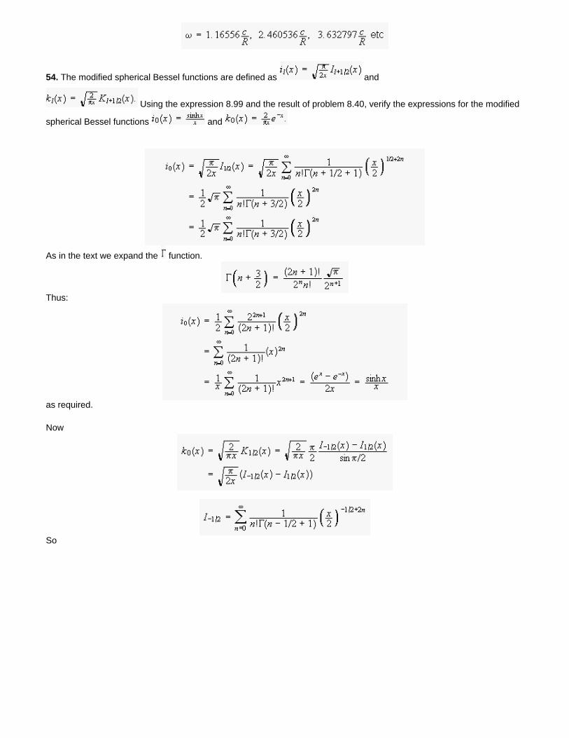
54. The modified spherical Bessel functions are defined as and
Using the expression 8.99 and the result of problem 8.40, verify the expressions for the modified
spherical Bessel functions and
As in the text we expand the function.
Thus:
as required.
Now
So
Thus
QED
Use proof by induction to show that
From the recursion relation in Problem 50 with
so the formula works for Now assume it works for some value Using the recursion relations, we have:
So the result is true for Thus it is true for all
55. We may model the force between particles in an atomic nucleus by a 3-D square well potential
with for Schrodinger's equation for this system takes the form:
Write the differential operator in spherical coordinates and show that the solution may be written in terms of spherical Bessel functions. Find the energy of the lowest energy level.
The equation is of the form (8.114) in the text and thus the solution is
where
inside the well. Outside the well which is imaginary if is negative (a bound state), and we need a
solution that decays exponentially. That solution is the spherical function (compare equation 8.105),
The boundary conditions are continuity of both and Thus
and
This is a transcendental equation for the energy values Let and Then
and
We use the recursion relations to eliminate the derivatives:
A factor of cancels, leaving
or
For we insert the explicit expressions for the Bessel functions, using equations (8.124) and (8.125)
Now using the result of problem 54
and

Thus the eigenvalue equation becomes:
Rearranging:
The plot shows the two sides of equation (1 Pr55) for The solutions are at , 0.5,
0.877565, and Thus the lowest energy level is:
Plot with
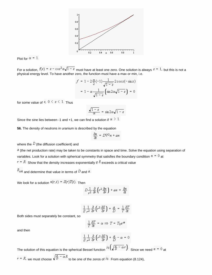
Plot for
For a solution, must have at least one zero. One solution is always but this is not a physical energy level. To have another zero, the function must have a max or min, i.e.
for some value of Thus
Since the sine lies between -1 and +1, we can find a solution if
56. The density of neutrons in uranium is described by the equation
where the (the diffusion coefficient) and
(the net production rate) may be taken to be constants in space and time. Solve the equation using separation of
variables. Look for a solution with spherical symmetry that satisfies the boundary condition at
Show that the density increases exponentially if exceeds a critical value
and determine that value in terms of and
We look for a solution Then
Both sides must separately be constant, so
and then
The solution of this equation is the spherical Bessel function Since we need at
we must choose to be one of the zeros of From equation (8.124),
and thus the first zero is at Thus
The density increases exponentially if or
This document created by Scientific WorkPlace 4.1.
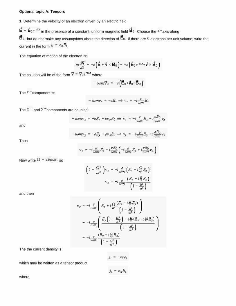
Optional topic A: Tensors
1. Determine the velocity of an electron driven by an electric field
in the presence of a constant, uniform magnetic field Choose the axis along
but do not make any assumptions about the direction of If there are electrons per unit volume, write the
current in the form .
The equation of motion of the electron is:
The solution will be of the form where
The component is:
The and components are coupled:
and
Thus
Now write so
and then
The the current density is
which may be written as a tensor product
where
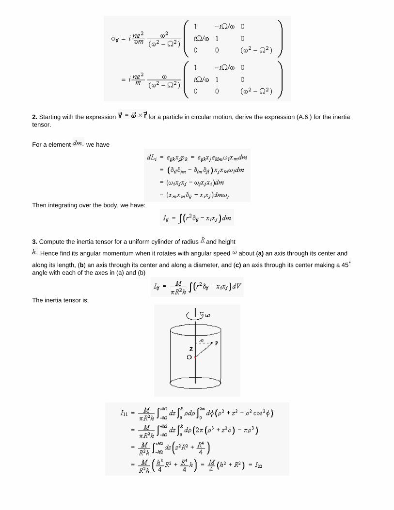
2. Starting with the expression for a particle in circular motion, derive the expression (A.6 ) for the inertia tensor.
For a element we have
Then integrating over the body, we have:
3. Compute the inertia tensor for a uniform cylinder of radius and height
Hence find its angular momentum when it rotates with angular speed about (a) an axis through its center and
along its length, (b) an axis through its center and along a diameter, and (c) an axis through its center making a 45 angle with each of the axes in (a) and (b)
The inertia tensor is:
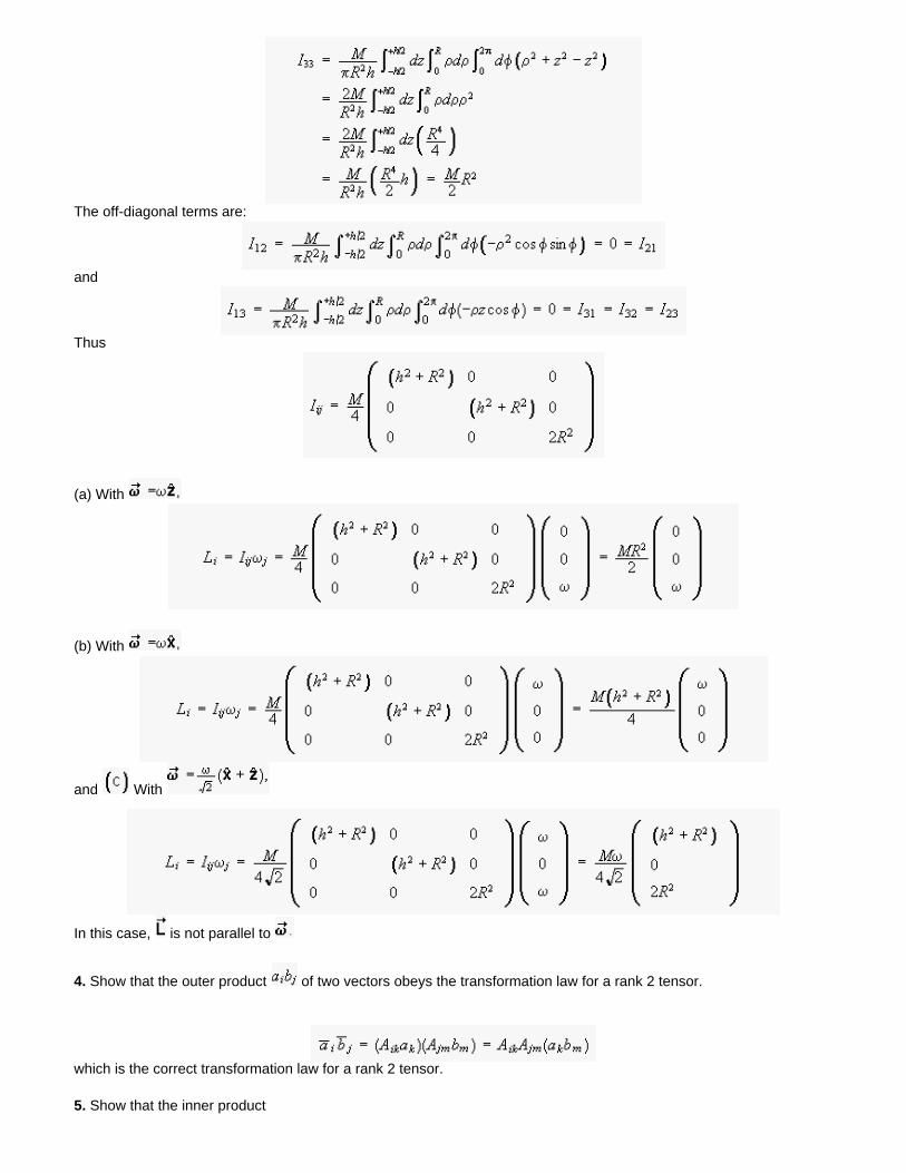
The off-diagonal terms are:
and
Thus
(a) With
(b) With
and With
In this case, is not parallel to
4. Show that the outer product of two vectors obeys the transformation law for a rank 2 tensor.
which is the correct transformation law for a rank 2 tensor.
5. Show that the inner product
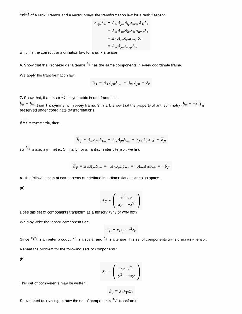
of a rank 3 tensor and a vector obeys the transformation law for a rank 2 tensor.
which is the correct transformation law for a rank 2 tensor.
6. Show that the Kroneker delta tensor has the same components in every coordinate frame.
We apply the transformation law:
7. Show that, if a tensor is symmetric in one frame, i.e.
then it is symmetric in every frame. Similarly show that the property of anti-symmetry ( is preserved under coordinate trasnformations.
If is symmetric, then:
so is also symmetric. Similarly, for an antisymmteric tensor, we find
8. The following sets of components are defined in 2-dimensional Cartesian space:
(a)
Does this set of components transform as a tensor? Why or why not?
We may write the tensor components as:
Since is an outer product, is a scalar and is a tensor, this set of components transforms as a tensor.
Repeat the problem for the following sets of components:
(b)
This set of components may be written:
So we need to investigate how the set of components transforms.
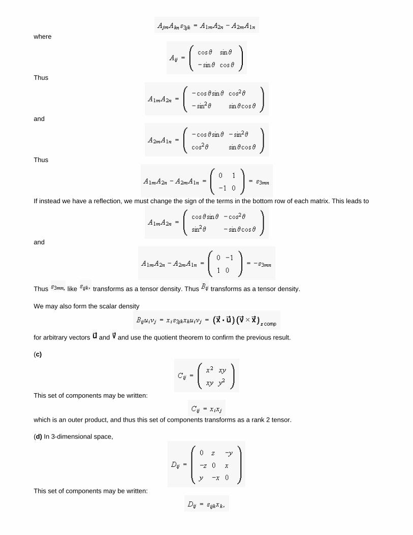
where
Thus
and
Thus
If instead we have a reflection, we must change the sign of the terms in the bottom row of each matrix. This leads to
and
Thus like transforms as a tensor density. Thus transforms as a tensor density.
We may also form the scalar density
for arbitrary vectors and and use the quotient theorem to confirm the previous result.
(c)
This set of components may be written:
which is an outer product, and thus this set of components transforms as a rank 2 tensor.
(d) In 3-dimensional space,
This set of components may be written:
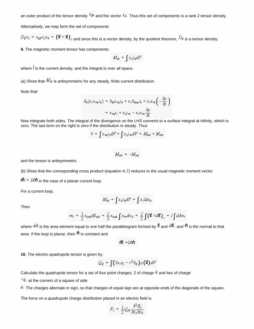
an outer product of the tensor density and the vector Thus this set of components is a rank 2 tensor density.
Alternatively, we may form the set of components
and since this is a vector density, by the quotient theorem, is a tensor density.
9. The magnetic moment tensor has components:
where is the current density, and the integral is over all space.
(a) Show that is antisymmetric for any steady, finite current distribution.
Note that:
Now integrate both sides. The integral of the divergence on the LHS converts to a surface integral at infinity, which is zero. The last term on the right is zero if the distribution is steady. Thus
and the tensor is antisymmetric.
(b) Show that the corresponding cross product (equation A.7) reduces to the usual magnetic moment vector
in the case of a planar current loop.
For a current loop,
Then
where is the area element equal to one half the parallelogram formed by and and is the normal to that
area. If the loop is planar, then is constant and
10. The electric quadrupole tensor is given by:
Calculate the quadrupole tensor for a set of four point charges, 2 of charge and two of charge
at the corners of a square of side
The charges alternate in sign, so that charges of equal sign are at opposite ends of the diagonals of the square.
The force on a quadrupole charge distribution placed in an electric field is
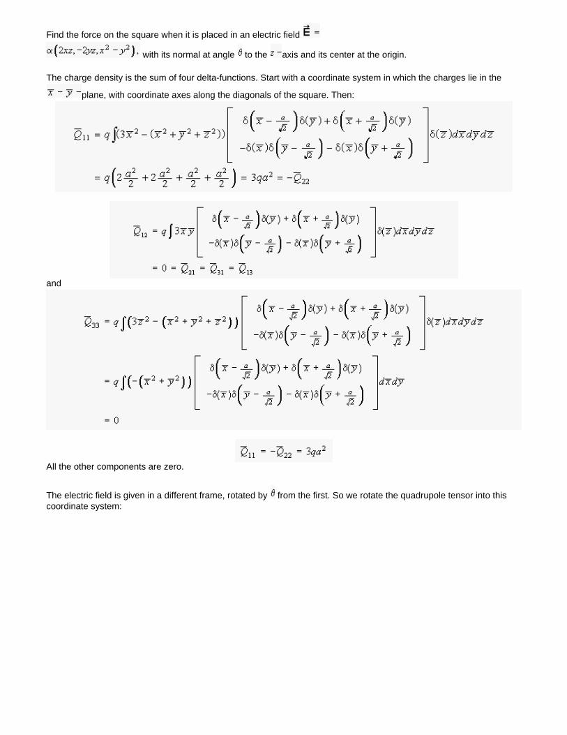
Find the force on the square when it is placed in an electric field
with its normal at angle to the axis and its center at the origin.
The charge density is the sum of four delta-functions. Start with a coordinate system in which the charges lie in the
plane, with coordinate axes along the diagonals of the square. Then:
and
All the other components are zero.
The electric field is given in a different frame, rotated by from the first. So we rotate the quadrupole tensor into this coordinate system:
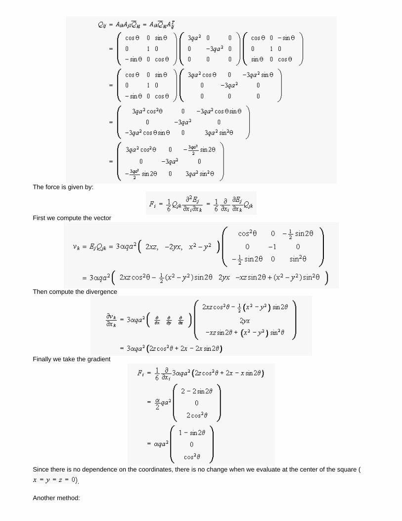
The force is given by:
First we compute the vector
Then compute the divergence
Finally we take the gradient
Since there is no dependence on the coordinates, there is no change when we evaluate at the center of the square (
.
Another method:
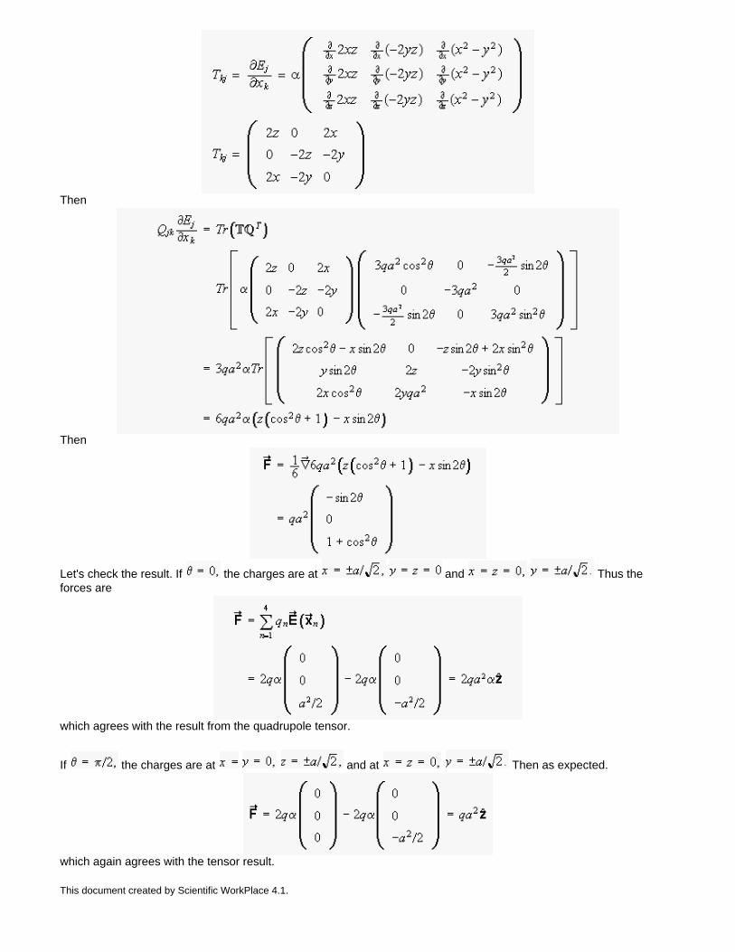
Then
Then
Let's check the result. If the charges are at and Thus the forces are
which agrees with the result from the quadrupole tensor.
If the charges are at and at Then as expected.
which again agrees with the tensor result.
This document created by Scientific WorkPlace 4.1.
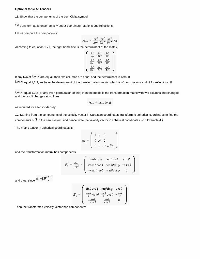
Optional topic A: Tensors
11. Show that the components of the Levi-Civita symbol
transform as a tensor density under coordinate rotations and reflections.
Let us compute the components:
According to equation 1.71, the right hand side is the determinant of the matrix,
If any two of are equal, then two columns are equal and the determinant is zero. If
equal 1,2,3, we have the determinant of the transformation matrix, which is +1 for rotations and -1 for reflections. If
equal 1,3,2 (or any even permutation of this) then the matrix is the transformation matrix with two columns interchanged, and the result changes sign. Thus
as required for a tensor density.
12. Starting from the components of the velocity vector in Cartesian coordinates, transform to spherical coordinates to find the
components of in the new system, and hence write the velocity vector in spherical coordinates. (c.f. Example 4.)
The metric tensor in spherical coordinates is:
and the transformation matrix has components:
and thus, since
Then the transformed velocity vector has components:
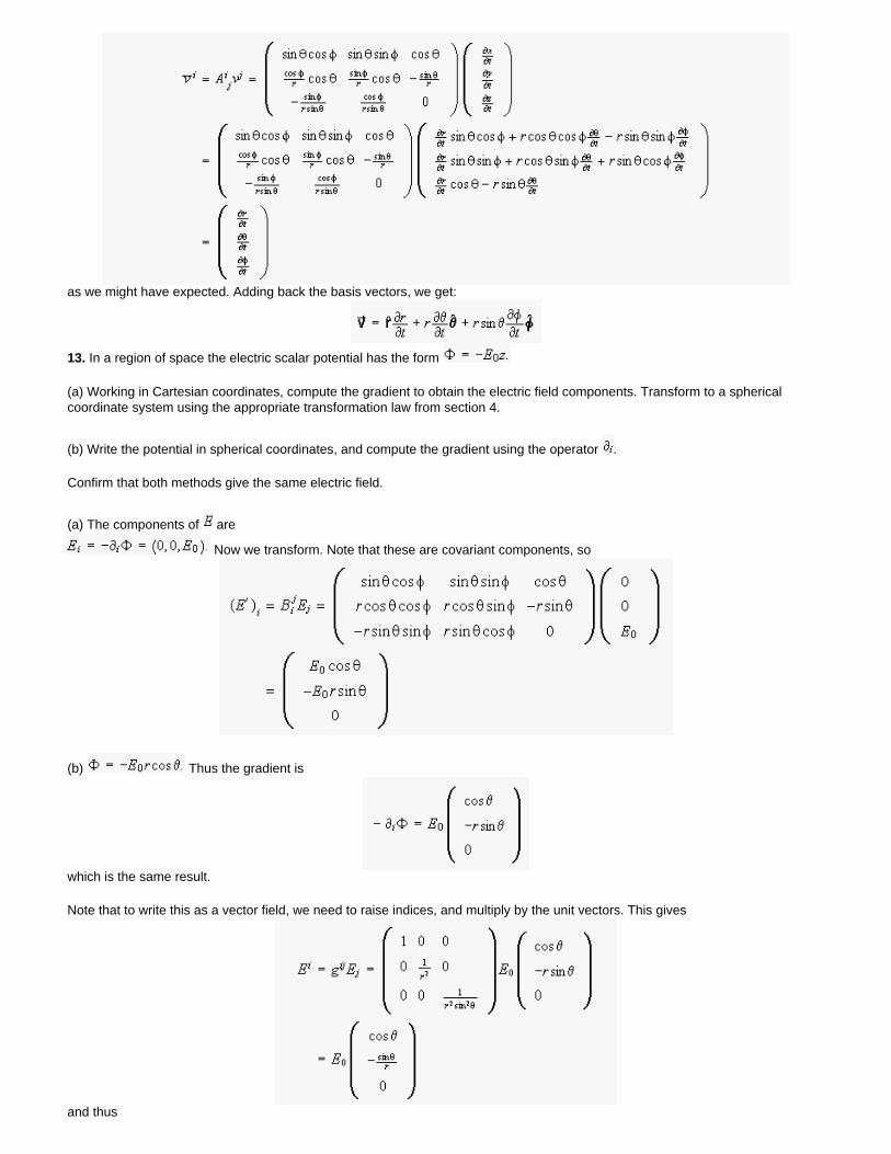
as we might have expected. Adding back the basis vectors, we get:
13. In a region of space the electric scalar potential has the form
(a) Working in Cartesian coordinates, compute the gradient to obtain the electric field components. Transform to a spherical coordinate system using the appropriate transformation law from section 4.
(b) Write the potential in spherical coordinates, and compute the gradient using the operator .
Confirm that both methods give the same electric field.
(a) The components of are
Now we transform. Note that these are covariant components, so
(b) Thus the gradient is
which is the same result.
Note that to write this as a vector field, we need to raise indices, and multiply by the unit vectors. This gives
and thus
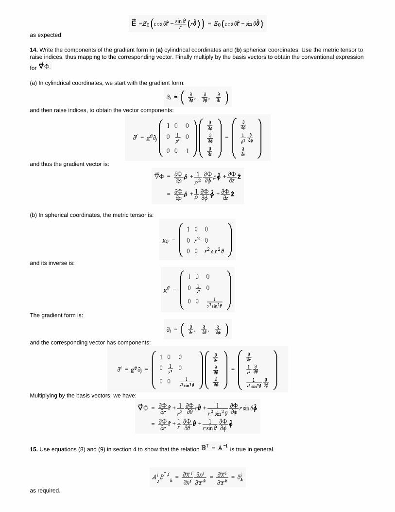
as expected.
14. Write the components of the gradient form in (a) cylindrical coordinates and (b) spherical coordinates. Use the metric tensor to raise indices, thus mapping to the corresponding vector. Finally multiply by the basis vectors to obtain the conventional expression
for
(a) In cylindrical coordinates, we start with the gradient form:
and then raise indices, to obtain the vector components:
and thus the gradient vector is:
(b) In spherical coordinates, the metric tensor is:
and its inverse is:
The gradient form is:
and the corresponding vector has components:
Multiplying by the basis vectors, we have:
15. Use equations (8) and (9) in section 4 to show that the relation is true in general.
as required.
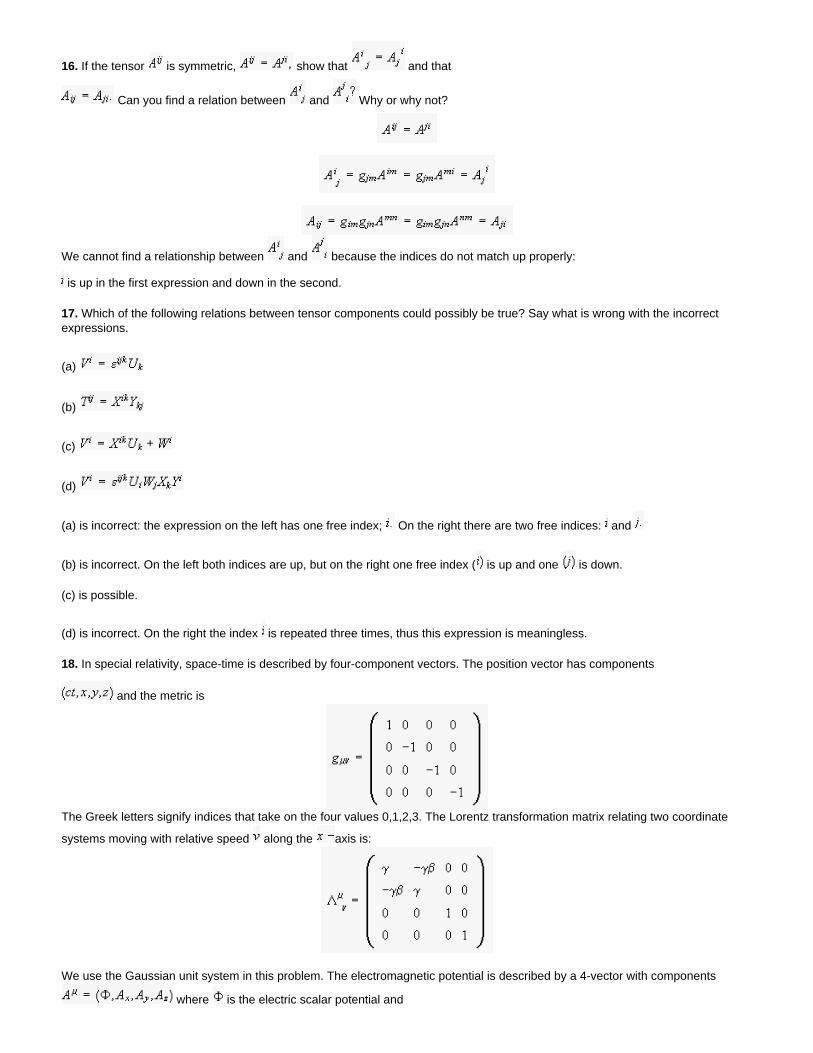
16. If the tensor is symmetric, show that and that
Can you find a relation between and Why or why not?
We cannot find a relationship between and because the indices do not match up properly:
is up in the first expression and down in the second.
17. Which of the following relations between tensor components could possibly be true? Say what is wrong with the incorrect expressions.
(a)
(b)
(c)
(d)
(a) is incorrect: the expression on the left has one free index; On the right there are two free indices: and
(b) is incorrect. On the left both indices are up, but on the right one free index ( is up and one is down.
(c) is possible.
(d) is incorrect. On the right the index is repeated three times, thus this expression is meaningless.
18. In special relativity, space-time is described by four-component vectors. The position vector has components
and the metric is
The Greek letters signify indices that take on the four values 0,1,2,3. The Lorentz transformation matrix relating two coordinate
systems moving with relative speed along the axis is:
We use the Gaussian unit system in this problem. The electromagnetic potential is described by a 4-vector with components
where is the electric scalar potential and
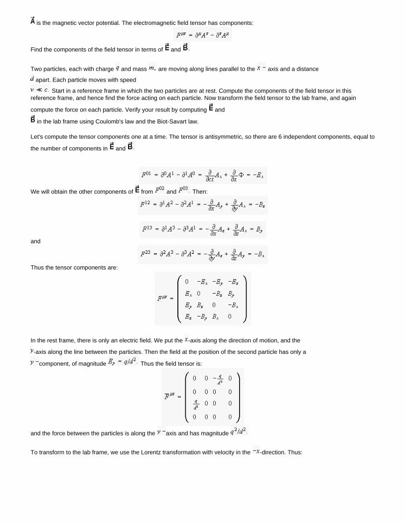
is the magnetic vector potential. The electromagnetic field tensor has components:
Find the components of the field tensor in terms of and
Two particles, each with charge and mass are moving along lines parallel to the axis and a distance
apart. Each particle moves with speed
Start in a reference frame in which the two particles are at rest. Compute the components of the field tensor in this reference frame, and hence find the force acting on each particle. Now transform the field tensor to the lab frame, and again
compute the force on each particle. Verify your result by computing and
in the lab frame using Coulomb's law and the Biot-Savart law.
Let's compute the tensor components one at a time. The tensor is antisymmetric, so there are 6 independent components, equal to
the number of components in and
We will obtain the other components of from and Then:
and
Thus the tensor components are:
In the rest frame, there is only an electric field. We put the -axis along the direction of motion, and the
-axis along the line between the particles. Then the field at the position of the second particle has only a
component, of magnitude Thus the field tensor is:
and the force between the particles is along the axis and has magnitude
To transform to the lab frame, we use the Lorentz transformation with velocity in the -direction. Thus:
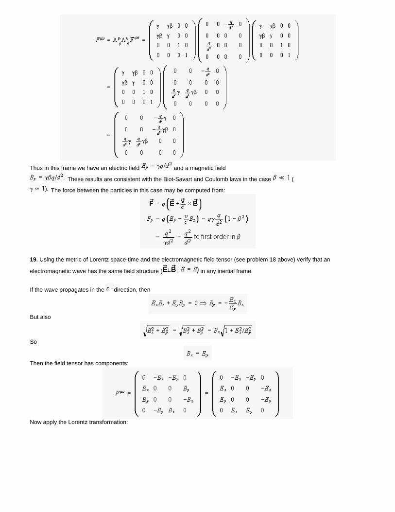
Thus in this frame we have an electric field and a magnetic field
These results are consistent with the Biot-Savart and Coulomb laws in the case (
The force between the particles in this case may be computed from:
19. Using the metric of Lorentz space-time and the electromagnetic field tensor (see problem 18 above) verify that an
electromagnetic wave has the same field structure ( in any inertial frame.
If the wave propagates in the direction, then
But also
So
Then the field tensor has components:
Now apply the Lorentz transformation:
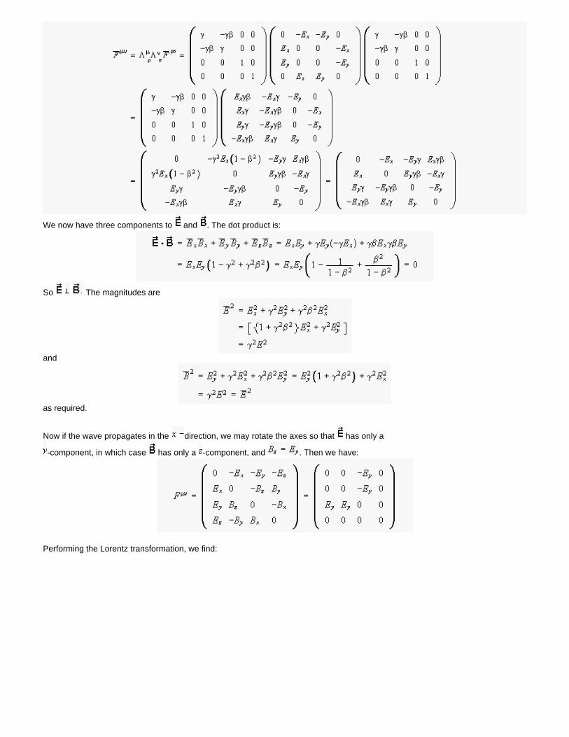
We now have three components to and . The dot product is:
So The magnitudes are
and
as required.
Now if the wave propagates in the direction, we may rotate the axes so that has only a
-component, in which case has only a -component, and . Then we have:
Performing the Lorentz transformation, we find:
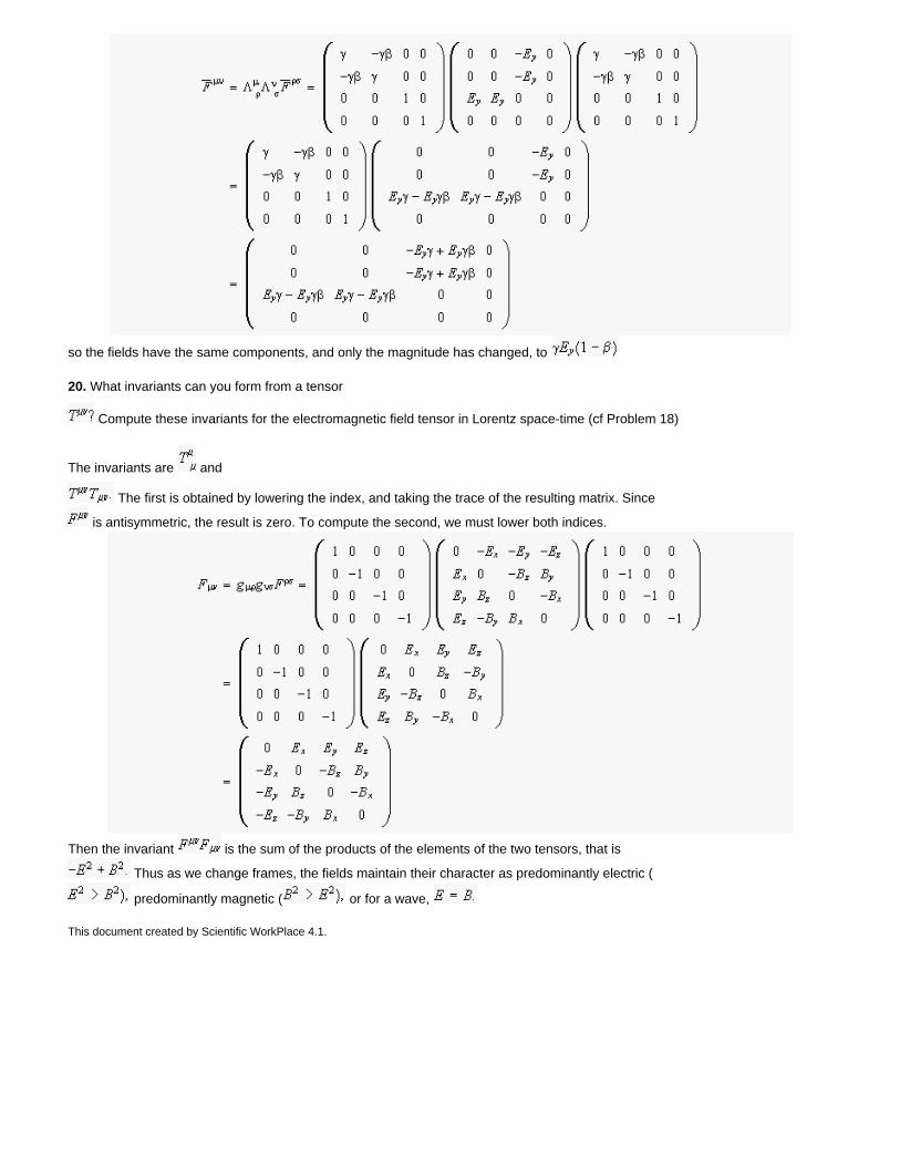
so the fields have the same components, and only the magnitude has changed, to
20. What invariants can you form from a tensor
Compute these invariants for the electromagnetic field tensor in Lorentz space-time (cf Problem 18)
The invariants are and
The first is obtained by lowering the index, and taking the trace of the resulting matrix. Since
is antisymmetric, the result is zero. To compute the second, we must lower both indices.
Then the invariant is the sum of the products of the elements of the two tensors, that is
Thus as we change frames, the fields maintain their character as predominantly electric (
predominantly magnetic ( or for a wave,
This document created by Scientific WorkPlace 4.1.
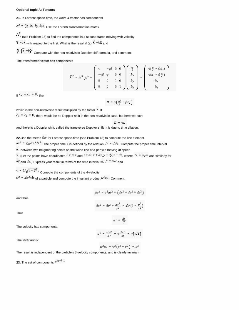
Optional topic A: Tensors
21. In Lorentz space-time, the wave 4-vector has components
Use the Lorentz transformation matrix
(see Problem 18) to find the components in a second frame moving with velocity
with respect to the first. What is the result if (a) and
Compare with the non-relativistic Doppler shift formula, and comment.
The transformed vector has components
If then
which is the non-relativistic result multiplied by the factor If
there would be no Doppler shift in the non-relativistic case, but here we have
and there is a Doppler shift, called the transverse Doppler shift. It is due to time dilation.
22.Use the metric for Lorentz space-time (see Problem 18) to compute the line element
The proper time is defined by the relation Compute the proper time interval
between two neighboring points on the world line of a particle moving at speed
(Let the points have coordinates and where and similarly for
and ) Express your result in terms of the time interval and
Compute the components of the 4-velocity
of a particle and compute the invariant product Comment.
and thus
Thus
The velocity has components:
The invariant is:
The result is independent of the particle's 3-velocity components, and is clearly invariant.
23. The set of components
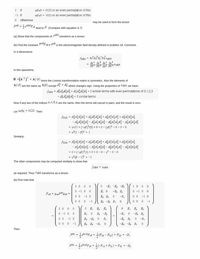
may be used to form the tensor
dual to (Compare with equation A.7)
(a) Show that the components of transform as a tensor.
(b) Find the invariant if is the electromagnetic field density defined in problem 18. Comment.
In 4-dimensions
In this spacetime,
since the Lorentz transformation matrix is symmetric. Also the elements of
are the same as except which changes sign. Using the properties of , we have:
Now if any two of the indices are the same, then the terms will cancel in pairs, and the result is zero.
Let Then
Similarly:
The other components may be computed similarly to show that
as required. Thus transforms as a tensor.
(b) First note that
Then
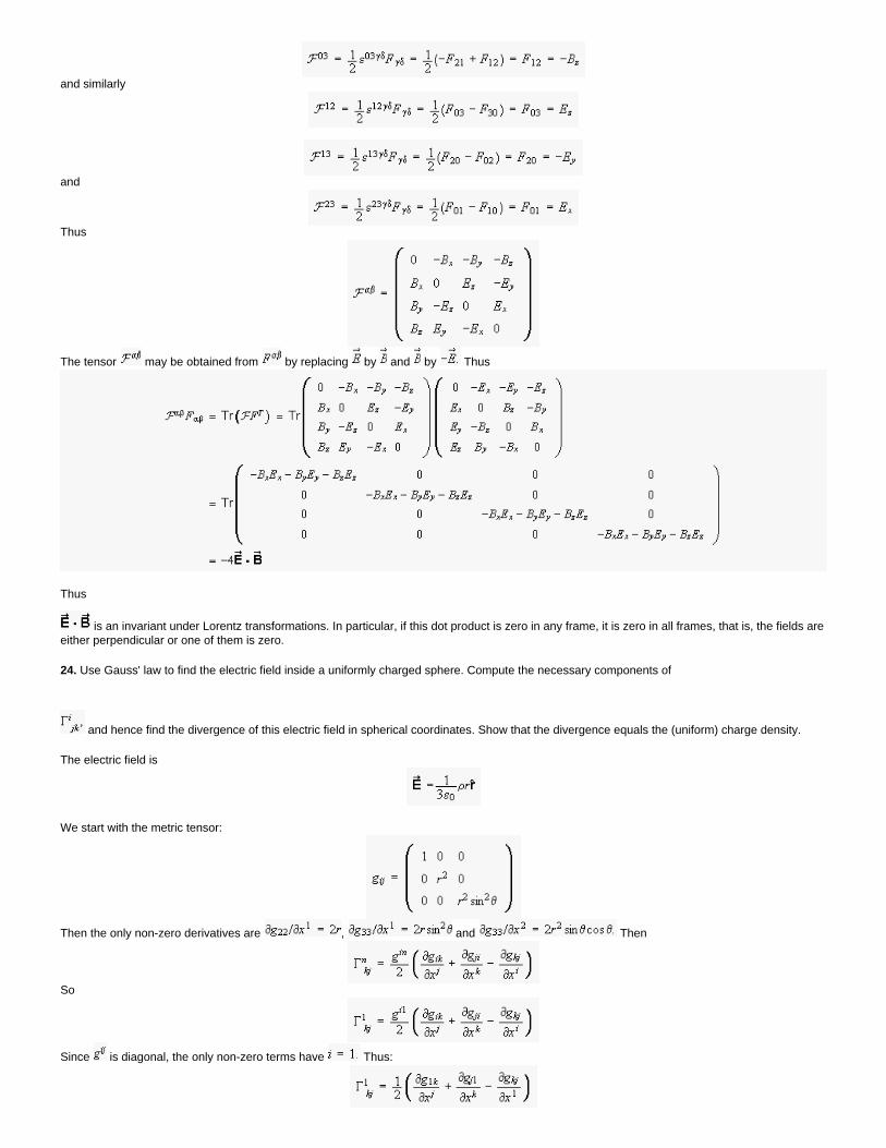
and similarly
and
Thus
The tensor may be obtained from by replacing by and by Thus
Thus
is an invariant under Lorentz transformations. In particular, if this dot product is zero in any frame, it is zero in all frames, that is, the fields are either perpendicular or one of them is zero.
24. Use Gauss' law to find the electric field inside a uniformly charged sphere. Compute the necessary components of
and hence find the divergence of this electric field in spherical coordinates. Show that the divergence equals the (uniform) charge density.
The electric field is
We start with the metric tensor:
Then the only non-zero derivatives are , and Then
So
Since is diagonal, the only non-zero terms have Thus:
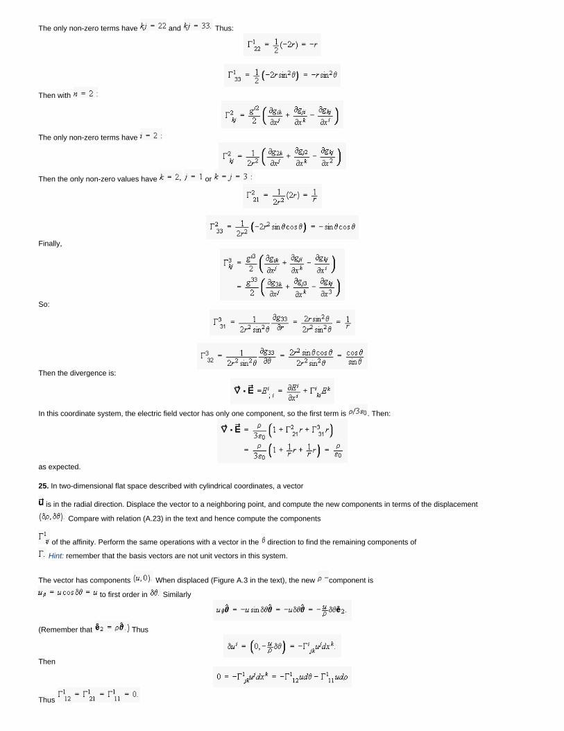
The only non-zero terms have and Thus:
Then with
The only non-zero terms have
Then the only non-zero values have or
Finally,
So:
Then the divergence is:
In this coordinate system, the electric field vector has only one component, so the first term is . Then:
as expected.
25. In two-dimensional flat space described with cylindrical coordinates, a vector
is in the radial direction. Displace the vector to a neighboring point, and compute the new components in terms of the displacement
Compare with relation (A.23) in the text and hence compute the components
of the affinity. Perform the same operations with a vector in the direction to find the remaining components of
Hint: remember that the basis vectors are not unit vectors in this system.
The vector has components When displaced (Figure A.3 in the text), the new component is
to first order in Similarly
(Remember that Thus
Then
Thus
So and
This document created by Scientific WorkPlace 4.1.
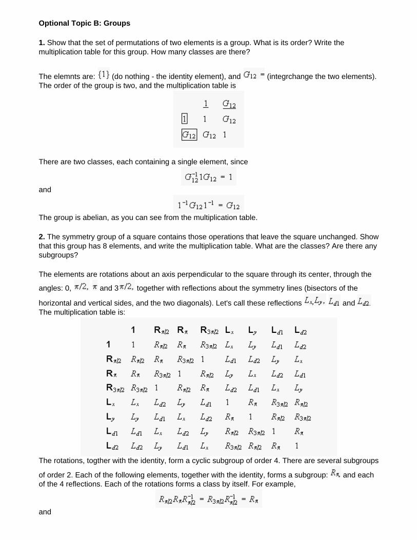
Optional Topic B: Groups
1. Show that the set of permutations of two elements is a group. What is its order? Write the multiplication table for this group. How many classes are there?
The elemnts are: (do nothing - the identity element), and (integrchange the two elements). The order of the group is two, and the multiplication table is
There are two classes, each containing a single element, since
and
The group is abelian, as you can see from the multiplication table.
2. The symmetry group of a square contains those operations that leave the square unchanged. Show that this group has 8 elements, and write the multiplication table. What are the classes? Are there any subgroups?
The elements are rotations about an axis perpendicular to the square through its center, through the
angles: 0, and 3 together with reflections about the symmetry lines (bisectors of the
horizontal and vertical sides, and the two diagonals). Let's call these reflections and The multiplication table is:
The rotations, togther with the identity, form a cyclic subgroup of order 4. There are several subgroups
of order 2. Each of the following elements, together with the identity, forms a subgroup: and each of the 4 reflections. Each of the rotations forms a class by itself. For example,
and
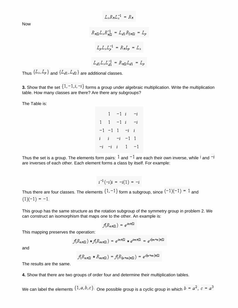
Now
Thus and are additional classes.
3. Show that the set forms a group under algebraic multiplication. Write the multiplication table. How many classes are there? Are there any subgroups?
The Table is:
Thus the set is a group. The elements form pairs: and are each their own inverse, while and are inverses of each other. Each element forms a class by itself. For example:
Thus there are four classes. The elements form a subgroup, since and
This group has the same structure as the rotation subgroup of the symmetry group in problem 2. We can construct an isomorphism that maps one to the other. An example is:
This mapping preserves the operation:
and
The results are the same.
4. Show that there are two groups of order four and determine their multiplication tables.
We can label the elements One possible group is a cyclic group in which
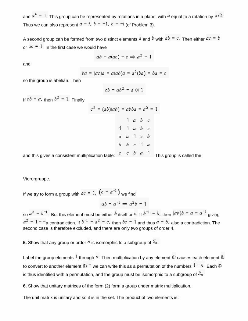
and This group can be represented by rotations in a plane, with equal to a rotation by
Thus we can also represent (cf Problem 3).
A second group can be formed from two distinct elements and with Then either
or In the first case we would have
and
so the group is abelian. Then
If then Finally
and this gives a consistent multiplication table: This group is called the
Vierergruppe.
If we try to form a group with we find
so But this element must be either itself or If then giving
a contradiction. If then and thus also a contradiction. The second case is therefore excluded, and there are only two groups of order 4.
5. Show that any group or order is isomorphic to a subgroup of
Label the group elements through Then multiplication by any element causes each element
to convert to another element we can write this as a permutation of the numbers Each
is thus identified with a permutation, and the group must be isomorphic to a subgroup of
6. Show that unitary matrices of the form (2) form a group under matrix multiplication.
The unit matrix is unitary and so it is in the set. The product of two elements is:
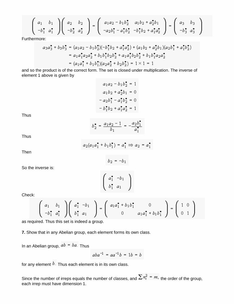
Furthermore:
and so the product is of the correct form. The set is closed under multiplication. The inverse of element 1 above is given by
Thus
Thus
Then
So the inverse is:
Check:
as required. Thus this set is indeed a group.
7. Show that in any Abelian group, each element forms its own class.
In an Abelian group, Thus
for any element Thus each element is in its own class.
Since the number of irreps equals the number of classes, and the order of the group, each irrep must have dimension 1.
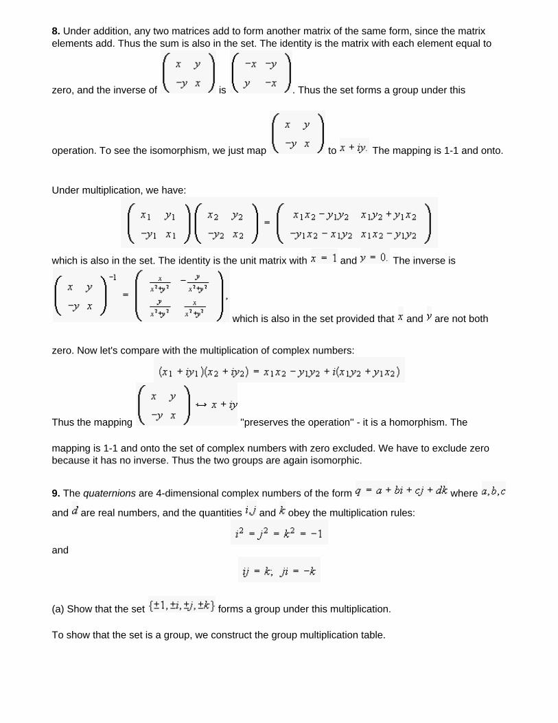
8. Under addition, any two matrices add to form another matrix of the same form, since the matrix elements add. Thus the sum is also in the set. The identity is the matrix with each element equal to
zero, and the inverse of is . Thus the set forms a group under this
operation. To see the isomorphism, we just map to The mapping is 1-1 and onto.
Under multiplication, we have:
which is also in the set. The identity is the unit matrix with and The inverse is
which is also in the set provided that and are not both
zero. Now let's compare with the multiplication of complex numbers:
Thus the mapping ''preserves the operation'' - it is a homorphism. The
mapping is 1-1 and onto the set of complex numbers with zero excluded. We have to exclude zero because it has no inverse. Thus the two groups are again isomorphic.
9. The quaternions are 4-dimensional complex numbers of the form where
and are real numbers, and the quantities and obey the multiplication rules:
and
(a) Show that the set forms a group under this multiplication.
To show that the set is a group, we construct the group multiplication table.
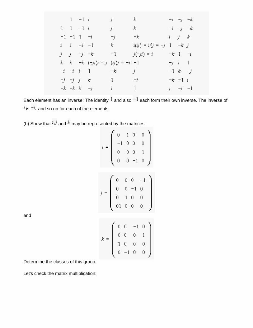
Each element has an inverse: The identity and also each form their own inverse. The inverse of
is and so on for each of the elements.
(b) Show that and may be represented by the matrices:
and
Determine the classes of this group.
Let's check the matrix multiplication:
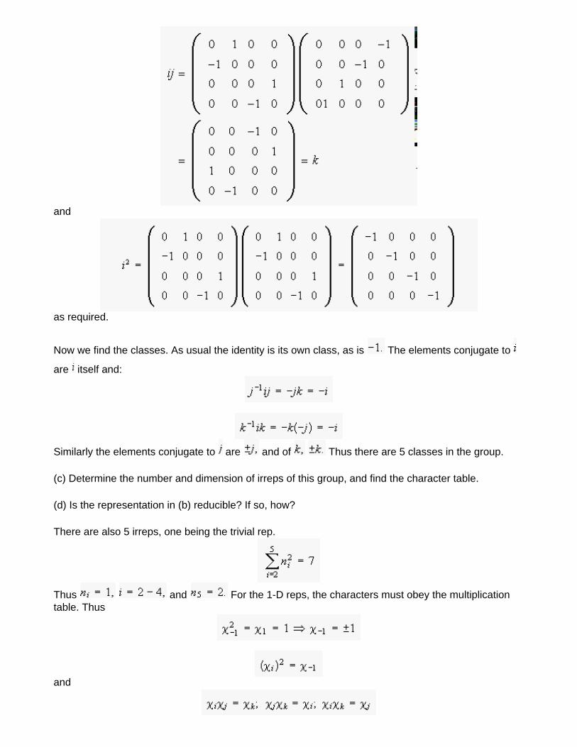
and
as required.
Now we find the classes. As usual the identity is its own class, as is The elements conjugate to
are itself and:
Similarly the elements conjugate to are and of Thus there are 5 classes in the group.
(c) Determine the number and dimension of irreps of this group, and find the character table.
(d) Is the representation in (b) reducible? If so, how?
There are also 5 irreps, one being the trivial rep.
Thus and For the 1-D reps, the characters must obey the multiplication table. Thus
and
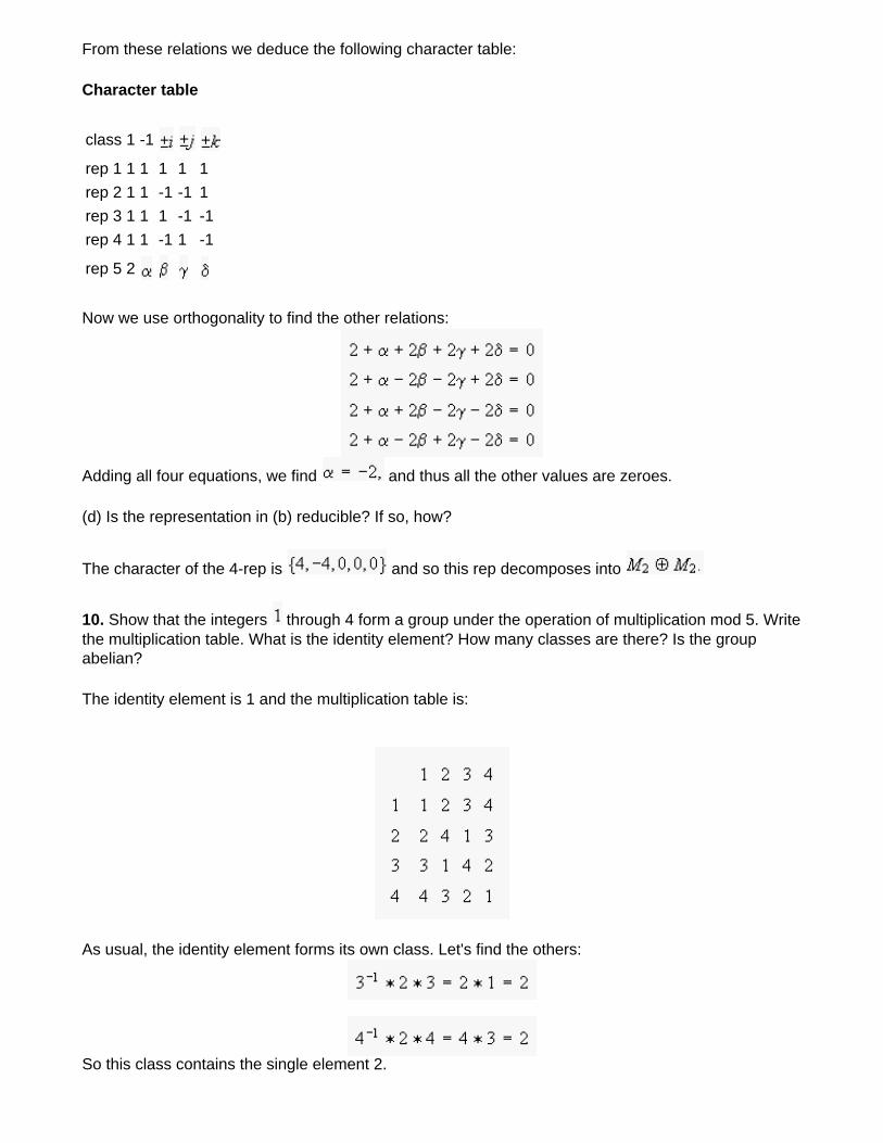
From these relations we deduce the following character table:
Character table
class 1 -1
rep 1 1 1 1 1 1rep 2 1 1 -1 -1 1rep 3 1 1 1 -1 -1rep 4 1 1 -1 1 -1
rep 5 2
Now we use orthogonality to find the other relations:
Adding all four equations, we find and thus all the other values are zeroes.
(d) Is the representation in (b) reducible? If so, how?
The character of the 4-rep is and so this rep decomposes into
10. Show that the integers through 4 form a group under the operation of multiplication mod 5. Write the multiplication table. What is the identity element? How many classes are there? Is the group abelian?
The identity element is 1 and the multiplication table is:
As usual, the identity element forms its own class. Let's find the others:
So this class contains the single element 2.
and
A similar thing happens with the last element. Thus each element forms its own class. The group is abelian.
This group is not isomorphic to the symmetry group of a square since the group structure is different.
11. Consider the mapping that maps the group of rationals to the group of integers by
Is the mapping a homomorphism? Why or why not?
It is not, because
whereas
The two results are not equal, and so the mapping is not a homomorphism.
This document created by Scientific WorkPlace 4.1.
Optional Topic B: Groups
12. Show that all elements in the same class have the same period.
If then
Continuing in this way, we find
Thus the period of equals the period of
13. Show that if a set of elements forms a class of a group then the set of the inverses
of is also a class.
The elements and where
are in the class Then
So
and thus
Thus the elements also form a class.
14. The center of a group is the set of elements that commute with every element in the group. Show
that the center is an Abelian subgroup of
First we show that the center is a subgroup. The identity is in because the identity commutes with
every element. Then if then for any element and Thus:
so is also in The inverse of is Any element for some in and thus
So also commutes with every and so is alos in the set. Thus is a subgroup.
The subgroup is abelian since every member commutes with every element in and thus with every
element in
The center always contains at least one element: the identity.
15. A homomorphism maps group to group The Kernel of the homomorphism is the set of all
elements of map to the identity element of Show that the Kernel is an invariant subgroup of
The identity is in
Thus is the identity of If and are in then
Thus is also in Also
But also
so
and is in Thus is a subgroup.
Now if the subgroup is invariant, then we must also have
and so is in and the subgroup is invariant.
16. A one-dimensional translation operator translates a function along the axis by an amount
where is a fixed step length:
(a) Show that the set of operators forms a group that may be represented by the complex numbers
What are the corresponding basis functions?
(b) Work out the orthogonality relation (14) for this representation, and comment. You will have to make some changes to account for the infinite order of the group.
First of all let's check the group properties. There is an identity: is the inverse of and
Thus the product of any two elements is also an element of the group. This demonstration also shows that
the group is abelian. The other group properties, such as associativity, follow trivially.
For an Abelian group, every irrep is 1-dimensional. The given set of numbers is an irrep, because they obey the group multiplication law:
The basis functions are Then
as required. Different irreps have different values of
The orthogonality relation is:
Because the order of the group is infinite and is a continuous variable, we have to change from the Kronecker delta to the delta function:
which is the expected completeness relation for Fourier series (see, e.g., equation 6.16).
(c) Now let the operator translate by an arbitrary amount What are the generators of this group?
We use the representation found above, with Then and near the identity
Thus the generators are the values and is already expressed in terms of its generators in this representation.
17. The operations that preserve the symmetry of this molecule are (i) rotation about its symmetry axis by
and (ii) Reflection about the symmetry plane. Each of these elements is is its own inverse,
and Thus the group has order 4.
Each element forms its own class, thus there are four irreps, each of dimension 1, and the character table is:
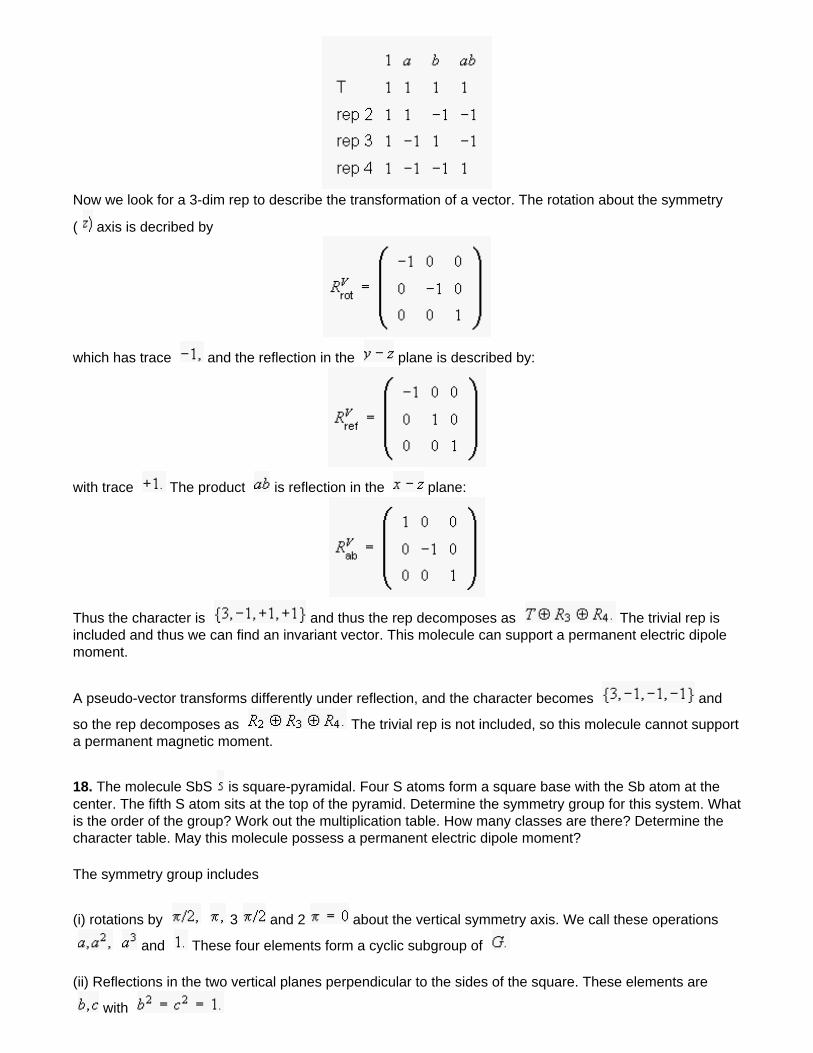
Now we look for a 3-dim rep to describe the transformation of a vector. The rotation about the symmetry
( axis is decribed by
which has trace and the reflection in the plane is described by:
with trace The product is reflection in the plane:
Thus the character is and thus the rep decomposes as The trivial rep is included and thus we can find an invariant vector. This molecule can support a permanent electric dipole moment.
A pseudo-vector transforms differently under reflection, and the character becomes and
so the rep decomposes as The trivial rep is not included, so this molecule cannot support a permanent magnetic moment.
18. The molecule SbS is square-pyramidal. Four S atoms form a square base with the Sb atom at the center. The fifth S atom sits at the top of the pyramid. Determine the symmetry group for this system. What is the order of the group? Work out the multiplication table. How many classes are there? Determine the character table. May this molecule possess a permanent electric dipole moment?
The symmetry group includes
(i) rotations by 3 and 2 about the vertical symmetry axis. We call these operations
and These four elements form a cyclic subgroup of
(ii) Reflections in the two vertical planes perpendicular to the sides of the square. These elements are
with
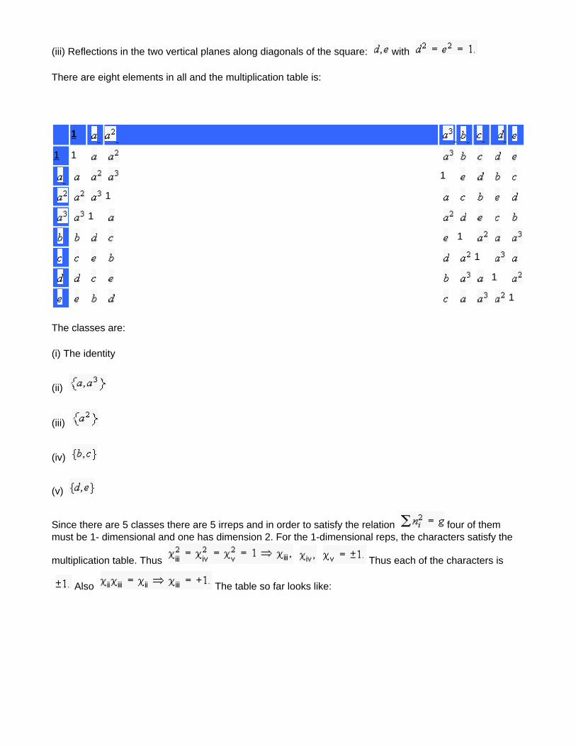
(iii) Reflections in the two vertical planes along diagonals of the square: with
There are eight elements in all and the multiplication table is:
1 1 1
1
1
1
1
1
1
1
The classes are:
(i) The identity
(ii)
(iii)
(iv)
(v)
Since there are 5 classes there are 5 irreps and in order to satisfy the relation four of them must be 1- dimensional and one has dimension 2. For the 1-dimensional reps, the characters satisfy the
multiplication table. Thus Thus each of the characters is
Also The table so far looks like:
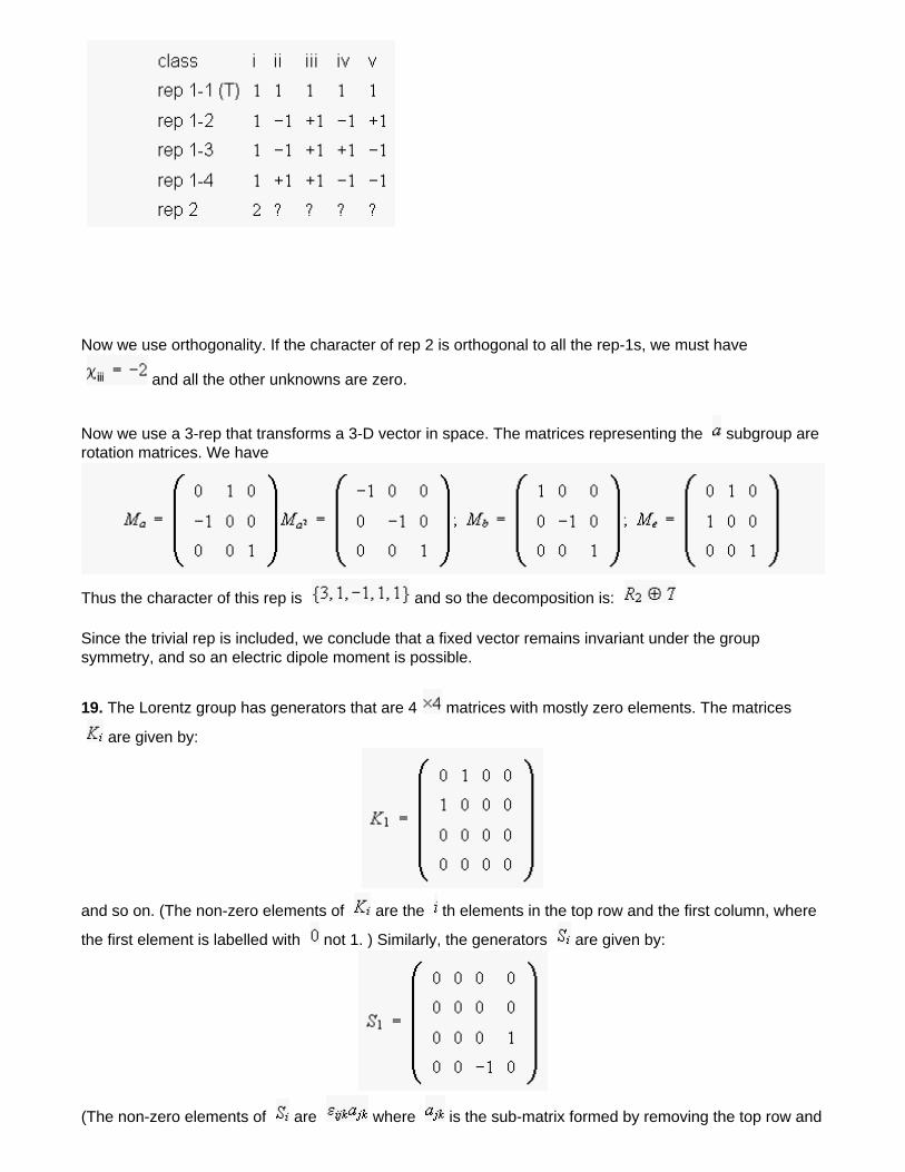
Now we use orthogonality. If the character of rep 2 is orthogonal to all the rep-1s, we must have
and all the other unknowns are zero.
Now we use a 3-rep that transforms a 3-D vector in space. The matrices representing the subgroup are rotation matrices. We have
Thus the character of this rep is and so the decomposition is:
Since the trivial rep is included, we conclude that a fixed vector remains invariant under the group symmetry, and so an electric dipole moment is possible.
19. The Lorentz group has generators that are 4 matrices with mostly zero elements. The matrices
are given by:
and so on. (The non-zero elements of are the th elements in the top row and the first column, where
the first element is labelled with not 1. ) Similarly, the generators are given by:
(The non-zero elements of are where is the sub-matrix formed by removing the top row and
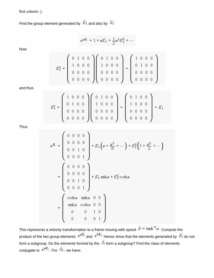
first column. ).
Find the group element generated by and also by
Now
and thus
Thus
This represents a velocity transformation to a frame moving with speed Compute the
product of the two group elements and Hence show that the elements generated by do not
form a subgroup. Do the elements formed by the form a subgroup? Find the class of elements
conjugate to For we have:
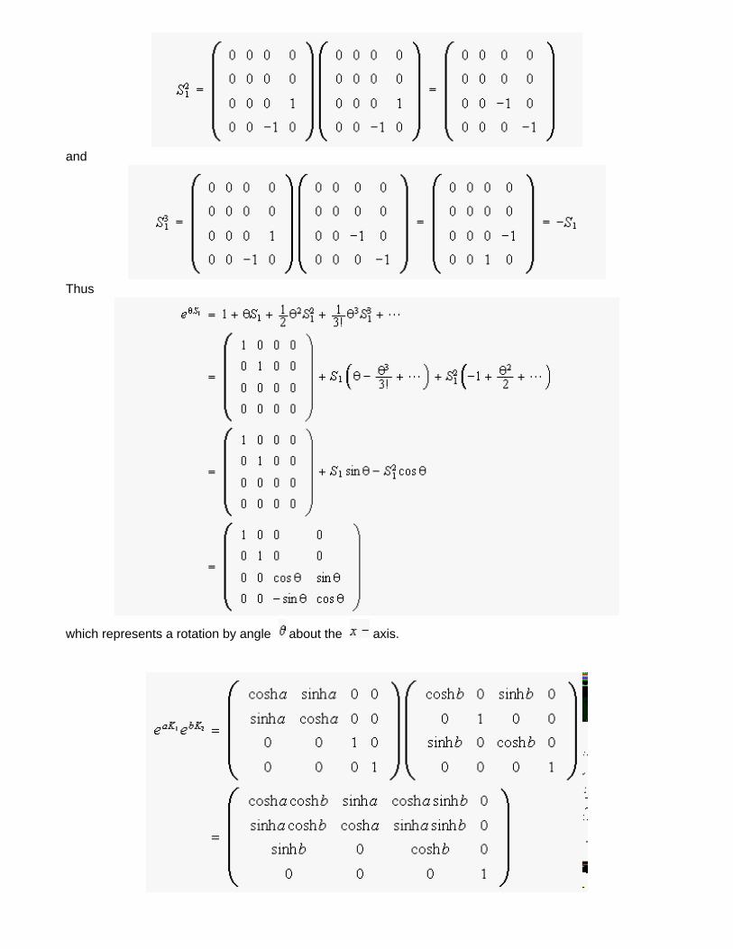
and
Thus
which represents a rotation by angle about the axis.
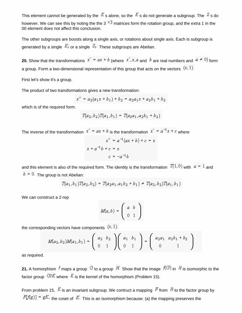
This element cannot be generated by the s alone, so the s do not generate a subgroup. The s do
however. We can see this by noting the the 3 matrices form the rotation group, and the extra 1 in the 00 element does not affect this conclusion.
The other subgroups are boosts along a single axis, or rotations about single axis. Each is subgroup is
generated by a single or a single These subgroups are Abelian.
20. Show that the transformations (where and are real numbers and form
a group. Form a two-dimensional representation of this group that acts on the vectors
First let's show it's a group.
The product of two transformations gives a new transformation:
which is of the required form.
The inverse of the transformation is the transformation where
and this element is also of the required form. The identity is the transformation with and
The group is not Abelian:
We can construct a 2-rep
the corresponding vectors have components
as required.
21. A homorphism maps a group to a group Show that the image in is isomorphic to the
factor group where is the kernel of the homorphism (Problem 15).
From problem 15, is an invariant subgroup. We contruct a mapping from to the factor group by
the coset of This is an isomorphism because: (a) the mapping preserves the
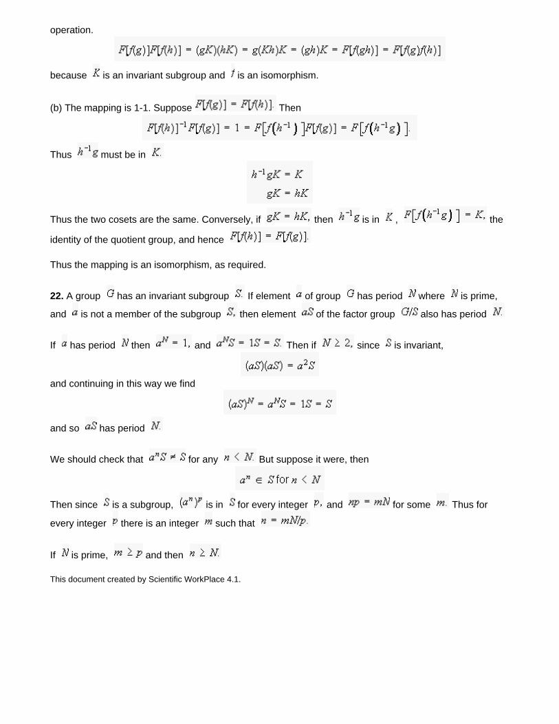
operation.
because is an invariant subgroup and is an isomorphism.
(b) The mapping is 1-1. Suppose Then
Thus must be in
Thus the two cosets are the same. Conversely, if then is in , the
identity of the quotient group, and hence
Thus the mapping is an isomorphism, as required.
22. A group has an invariant subgroup If element of group has period where is prime,
and is not a member of the subgroup then element of the factor group also has period
If has period then and Then if since is invariant,
and continuing in this way we find
and so has period
We should check that for any But suppose it were, then
Then since is a subgroup, is in for every integer and for some Thus for
every integer there is an integer such that
If is prime, and then
This document created by Scientific WorkPlace 4.1.
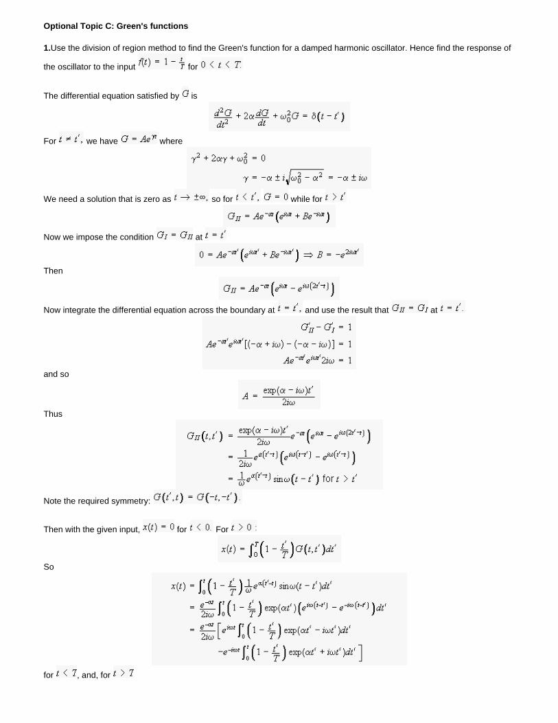
Optional Topic C: Green's functions
1.Use the division of region method to find the Green's function for a damped harmonic oscillator. Hence find the response of
the oscillator to the input for
The differential equation satisfied by is
For we have where
We need a solution that is zero as so for while for
Now we impose the condition at
Then
Now integrate the differential equation across the boundary at and use the result that at
and so
Thus
Note the required symmetry:
Then with the given input, for For
So
for , and, for
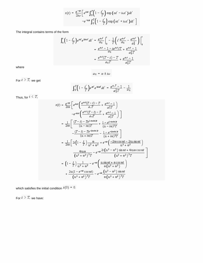
The integral contains terms of the form
where
For we get
Thus, for
which satisfies the initial condition
For we have:
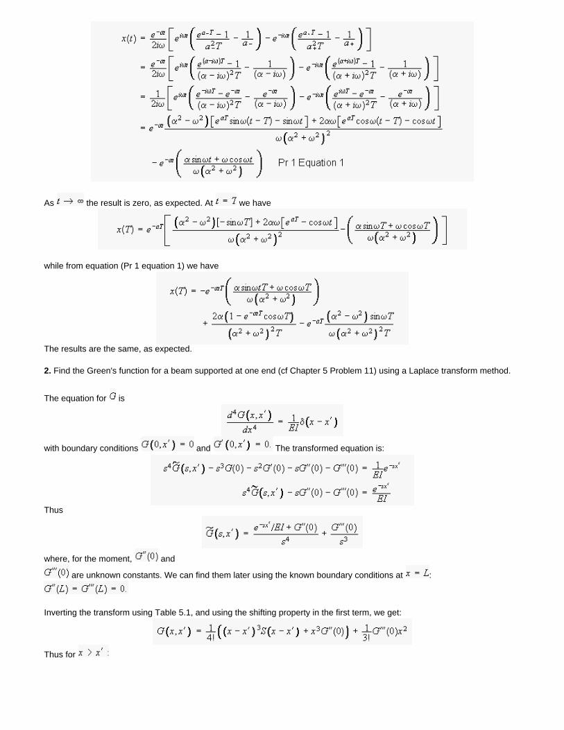
As the result is zero, as expected. At we have
while from equation (Pr 1 equation 1) we have
The results are the same, as expected.
2. Find the Green's function for a beam supported at one end (cf Chapter 5 Problem 11) using a Laplace transform method.
The equation for is
with boundary conditions and The transformed equation is:
Thus
where, for the moment, and
are unknown constants. We can find them later using the known boundary conditions at :
Inverting the transform using Table 5.1, and using the shifting property in the first term, we get:
Thus for
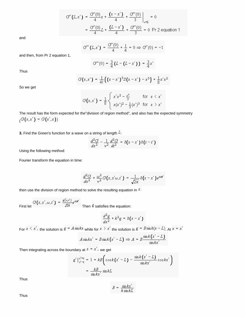
and
and then, from Pr 2 equation 1,
Thus
So we get
The result has the form expected for the"division of region method", and also has the expected symmetry
(
3. Find the Green's function for a wave on a string of length :
Using the following method:
Fourier transform the equation in time:
then use the division of region method to solve the resulting equation in
First let Then satisfies the equation:
For the solution is while for the solution is . At
Then integrating across the boundary at we get
Thus
Thus
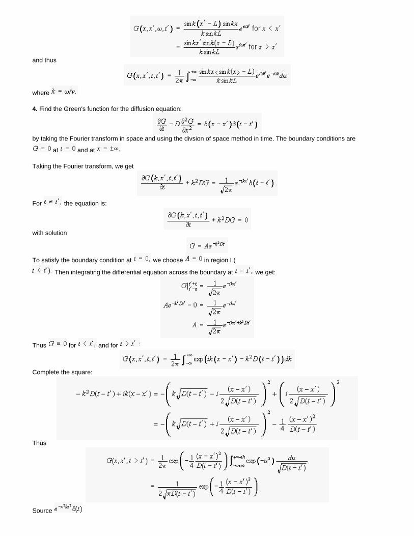
and thus
where
4. Find the Green's function for the diffusion equation:
by taking the Fourier transform in space and using the divsion of space method in time. The boundary conditions are
at and at
Taking the Fourier transform, we get
For the equation is:
with solution
To satisfy the boundary condition at we choose in region I (
Then integrating the differential equation across the boundary at we get:
Thus for and for
Complete the square:
Thus
Source
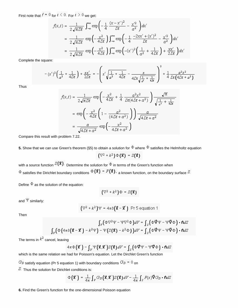
First note that for For we get:
Complete the square:
Thus
Compare this result with problem 7.22.
5. Show that we can use Green's theorem (§5) to obtain a solution for where satisfies the Helmholtz equation
with a source function Determine the solution for in terms of the Green's function when
satisfies the Dirichlet boundary conditions a known function, on the boundary surface
Define as the solution of the equation:
and similarly:
Then
The terms in cancel, leaving
which is the same relation we had for Poisson's equation. Let the Dirchlet Green's function
satisfy equation (Pr 5 equation 1) with boundary conditions on
Thus the solution for Dirichlet conditions is:
6. Find the Green's function for the one-dimensional Poisson equation
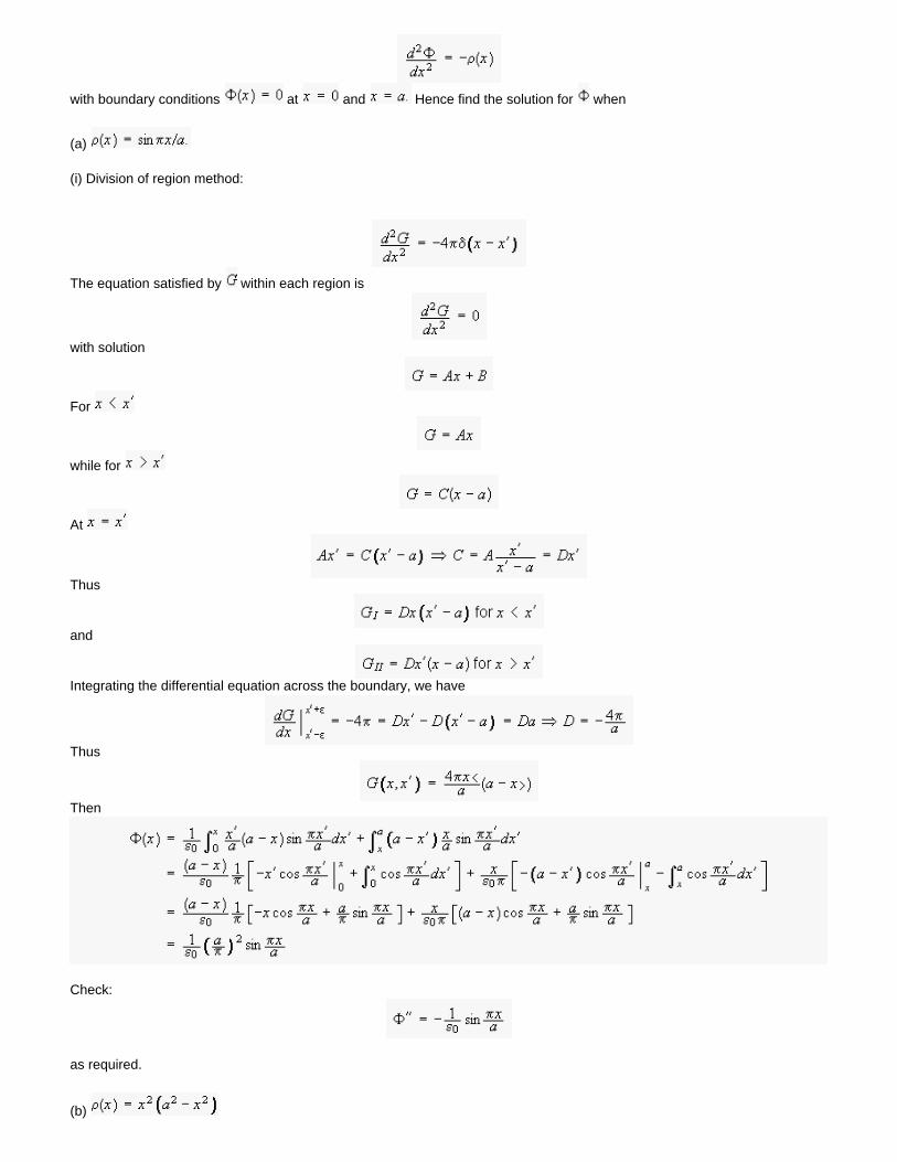
with boundary conditions at and Hence find the solution for when
(a)
(i) Division of region method:
The equation satisfied by within each region is
with solution
For
while for
At
Thus
and
Integrating the differential equation across the boundary, we have
Thus
Then
Check:
as required.
(b)
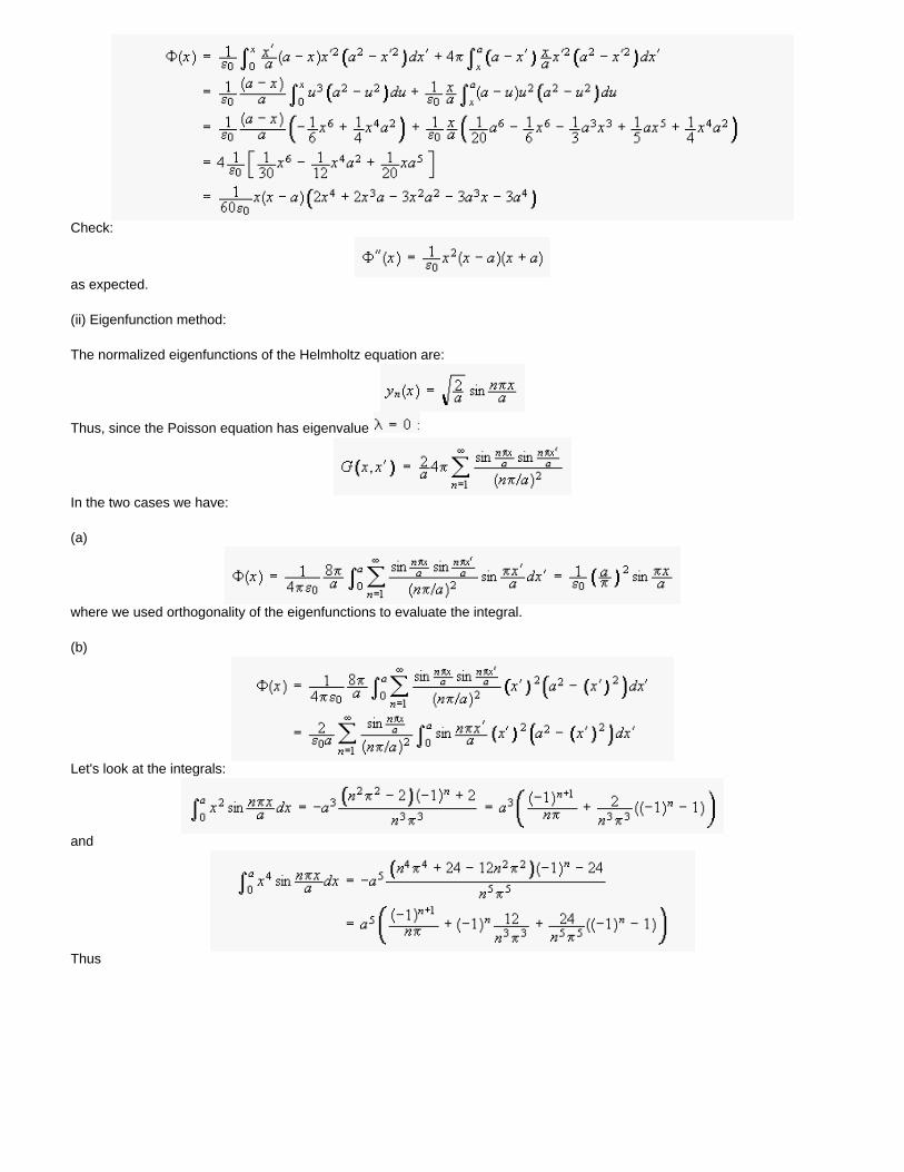
Check:
as expected.
(ii) Eigenfunction method:
The normalized eigenfunctions of the Helmholtz equation are:
Thus, since the Poisson equation has eigenvalue
In the two cases we have:
(a)
where we used orthogonality of the eigenfunctions to evaluate the integral.
(b)
Let's look at the integrals:
and
Thus
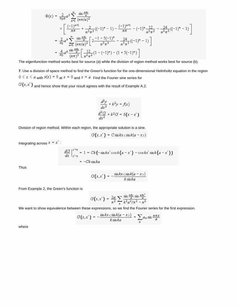
The eigenfunction method works best for source (a) while the division of region method works best for source (b).
7. Use a division of space method to find the Green's function for the one-dimensional Helmholtz equation in the region
with at and Find the Fourier sine series for
and hence show that your result agrees with the result of Example A.2.
Division of region method. Within each region, the appropriate solution is a sine.
Integrating across
Thus
From Example 2, the Green's function is
We want to show equivalence between these expressions, so we find the Fourier series for the first expression.
where
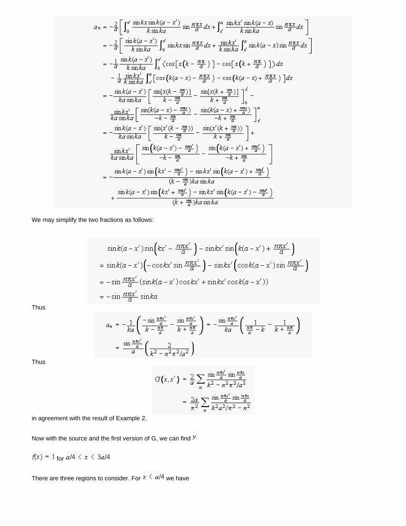
We may simplify the two fractions as follows:
Thus
Thus
in agreement with the result of Example 2.
Now with the source and the first version of G, we can find
for
There are three regions to consider. For we have
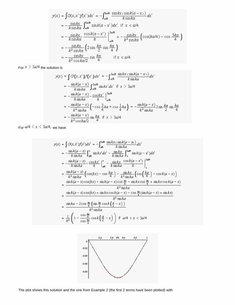
For the solution is
For we have
The plot shows this solution and the one from Example 2 (the first 2 terms have been plotted) with
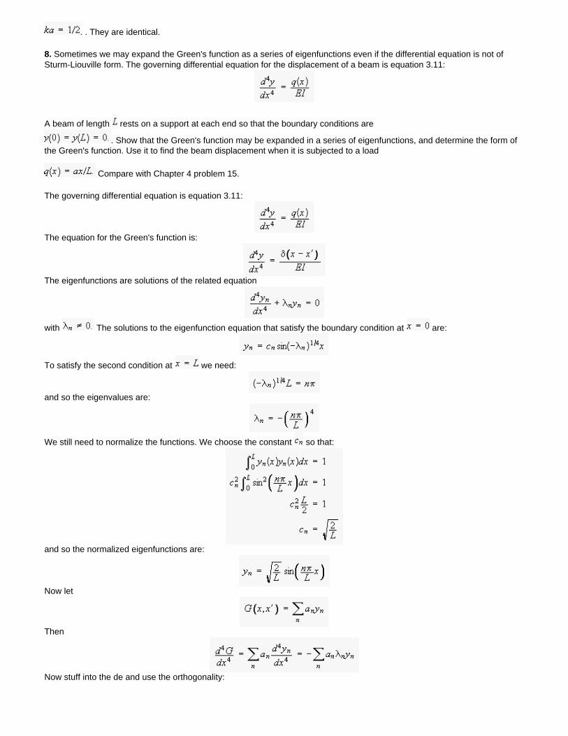
. . They are identical.
8. Sometimes we may expand the Green's function as a series of eigenfunctions even if the differential equation is not of Sturm-Liouville form. The governing differential equation for the displacement of a beam is equation 3.11:
A beam of length rests on a support at each end so that the boundary conditions are
. Show that the Green's function may be expanded in a series of eigenfunctions, and determine the form of the Green's function. Use it to find the beam displacement when it is subjected to a load
Compare with Chapter 4 problem 15.
The governing differential equation is equation 3.11:
The equation for the Green's function is:
The eigenfunctions are solutions of the related equation
with The solutions to the eigenfunction equation that satisfy the boundary condition at are:
To satisfy the second condition at we need:
and so the eigenvalues are:
We still need to normalize the functions. We choose the constant so that:
and so the normalized eigenfunctions are:
Now let
Then
Now stuff into the de and use the orthogonality:
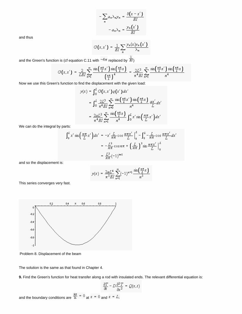
and thus
and the Green's function is (cf equation C.11 with replaced by )
Now we use this Green's function to find the displacement with the given load:
We can do the integral by parts:
and so the displacement is:
This series converges very fast.
Problem 8. Displacement of the beam
The solution is the same as that found in Chapter 4.
9. Find the Green's function for heat transfer along a rod with insulated ends. The relevant differential equation is:
and the boundary conditions are at and
. Treat the problem as a two-dimensional problem, and use method 1 in section C.4, dividing the region in time.
The differential equation for is
For we have:
Separate variables to find the eigenfunctions:
We choose the separation constant to be Then
and
So
To satisfy the boundary conditions at and we choose the cosine function, and the eigenvalues are
Then
Now we divide space in time. For . Thus we have:
where
Then equation () becomes
We multiply by and integrate along the rod. On the left, only one term survives the integration.
Now we may rewrite as
and integrate across the boundary at
Thus
and
The
term is just a constant corresponding to the initial uniform temperature of the rod. The result shows the expected
behavior: high frequency spatial variations (large are smoothed out faster than low frequency ones.
10.Verify that equation (C.34) gives the correct result in the limit from above.
Limit
Because of the exponential, as approaches zero the integral is dominated by values of near So expand
in a Taylor series:
Change variables to
Then
Now provided that remains positive, the upper limit in becomes infinite. Thus:
The second (and subsequent) integrals remain finite so long as
remains positive, so in the limit these terms go to zero.
This document created by Scientific WorkPlace 4.1.
Optional Topic C: Green's functions
11.Find the Green's function for the wave equation in three space dimensions, using spherical coordinates. The wave equation is:
where is the displacement,
is the Laplacian operator in three dimensions. Transform the equation in space and time, and solve for the .
The transformed equation is
which has the solution
as before, but here is the magnitude of the wave vector The solution is then:
The integrand has two poles at on the real axis. We want the result to be zero for and for
we must close upward, so the poles must be below the path of integration. Thus for we have:
where we used the result of Chapter 6, problem 13.
Then if the source is we get
Change variables to with fixed. Then
and
we have
As in the one-dimensional case, the displacement never goes negative.
12. Find the Dirichlet Green's function for the Helmholtz equation in a circular region of radius
. Obtain the result as a double sum over appropriate eigenfunctions.
The equation for is
where is a two-component vector The eigenfunction equation is:
As in Chapter we write the operator in polar coordinates to obtain:
Separating variables, we have:
Thus and
This is Bessel's equation (8.56) with solution
We must choose so that that is, the th zero of
Thus the eigenfunctions we need are
with eigenvalue Next we must normalize these functions. Since
and
(equation 8.96), the normalized eigenfunctions are
Thus from equation C.11 extended to two dimensions, the Green's function is:
As in the one-dimensional case, the solution does not exist if equals a resonant frequency
. Convince yourself that the result is dimensionally correct.
13. Find the Neumann Green's function for the one-dimensional Poisson equation:
with boundary conditions at and
Express your answer as a series of eigenfunctions. Hence find the potential if for
and zero otherwise, and the charge density is zero on the bounding surfaces ( at
and .
The eigenfunctions satisfy the equation:
with solutions and To satisfy the boundary conditions we choose the cosine and take
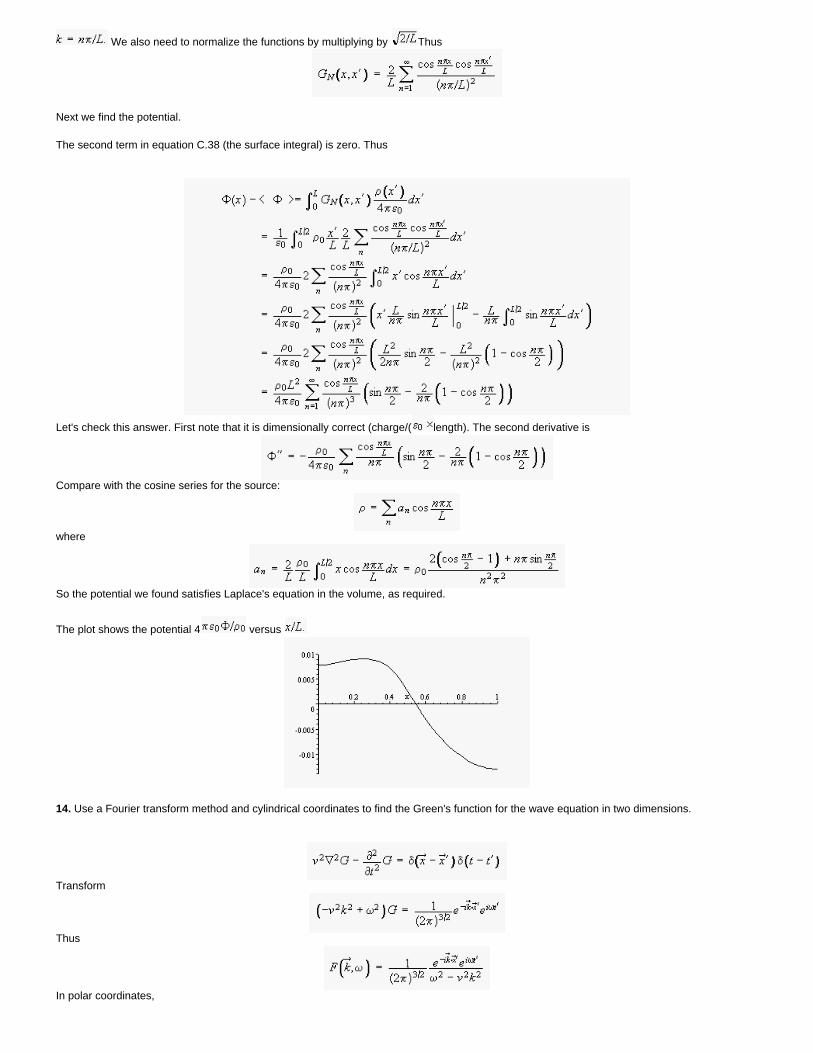
We also need to normalize the functions by multiplying by Thus
Next we find the potential.
The second term in equation C.38 (the surface integral) is zero. Thus
Let's check this answer. First note that it is dimensionally correct (charge/( length). The second derivative is
Compare with the cosine series for the source:
where
So the potential we found satisfies Laplace's equation in the volume, as required.
The plot shows the potential 4 versus
14. Use a Fourier transform method and cylindrical coordinates to find the Green's function for the wave equation in two dimensions.
Transform
Thus
In polar coordinates,
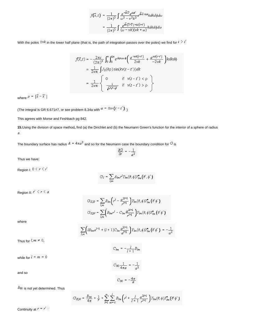
With the poles in the lower half plane (that is, the path of integration passes over the poles) we find for
where
(The integral is GR 6.671#7, or see problem 8.34a with )
This agrees with Morse and Feshbach pg 842.
15.Using the division of space method, find (a) the Dirichlet and (b) the Neumann Green's function for the interior of a sphere of radius
The boundary surface has radius and so for the Neumann case the boundary condition for is
Thus we have:
Region I:
Region II:
where
Thus for
while for
and so
is not yet determined. Thus
Continuity at
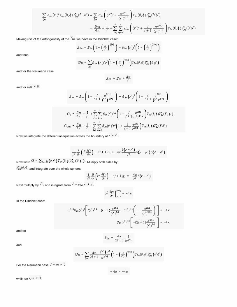
Making use of the orthogonality of the we have in the Dirichlet case:
and thus
and for the Neumann case
and for
Now we integrate the differential equation across the boundary at
Now write Multiply both sides by
and integrate over the whole sphere:
Next multiply by and integrate from to
In the Dirichlet case:
and so
and
For the Neumann case:
while for
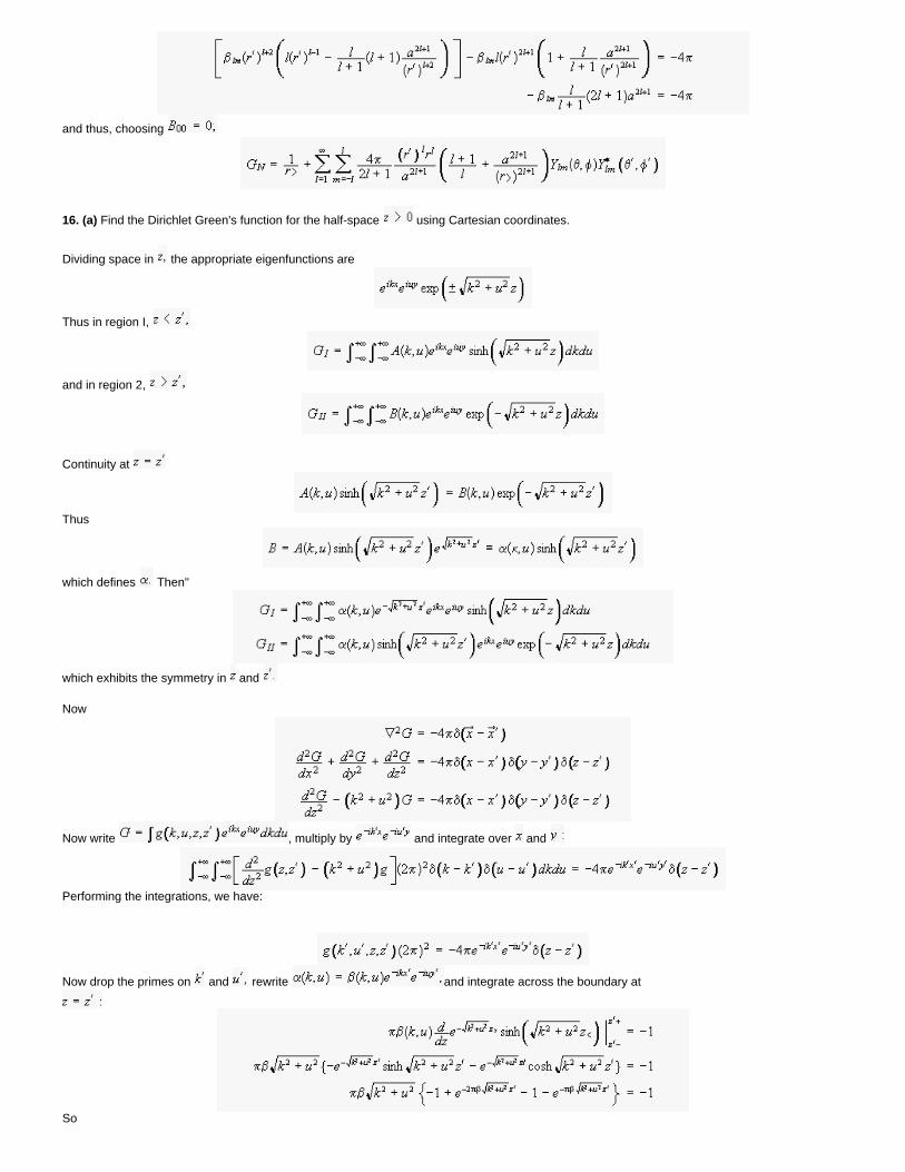
and thus, choosing
16. (a) Find the Dirichlet Green's function for the half-space using Cartesian coordinates.
Dividing space in the appropriate eigenfunctions are
Thus in region I,
and in region 2,
Continuity at
Thus
which defines Then''
which exhibits the symmetry in and
Now
Now write , multiply by and integrate over and
Performing the integrations, we have:
Now drop the primes on and rewrite and integrate across the boundary at
So
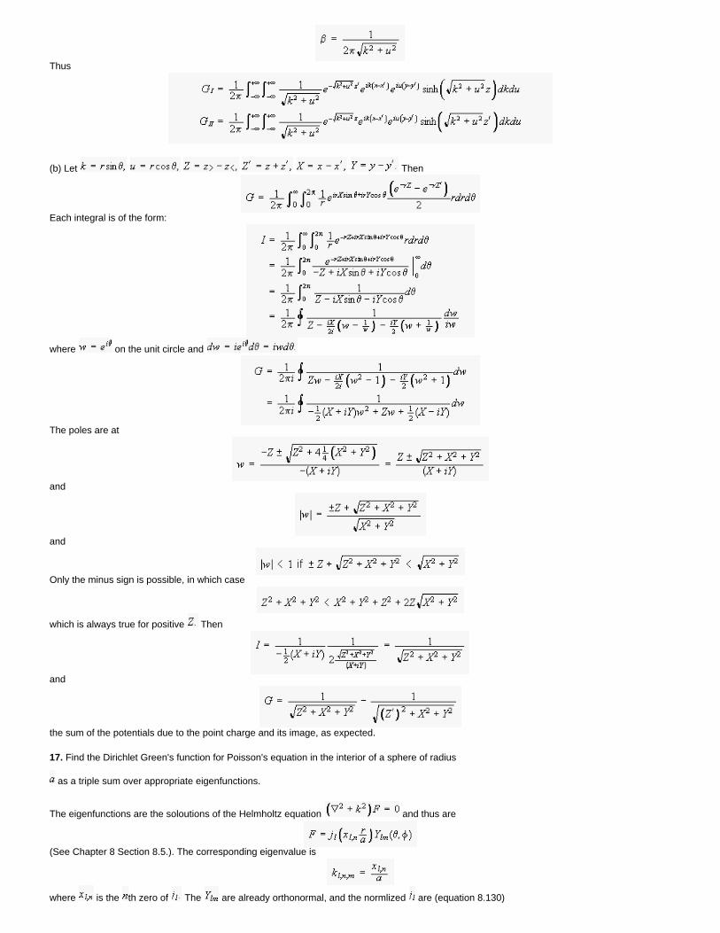
Thus
(b) Let Then
Each integral is of the form:
where on the unit circle and
The poles are at
and
and
Only the minus sign is possible, in which case
which is always true for positive Then
and
the sum of the potentials due to the point charge and its image, as expected.
17. Find the Dirichlet Green's function for Poisson's equation in the interior of a sphere of radius
as a triple sum over appropriate eigenfunctions.
The eigenfunctions are the soloutions of the Helmholtz equation and thus are
(See Chapter 8 Section 8.5.). The corresponding eigenvalue is
where is the th zero of The are already orthonormal, and the normlized are (equation 8.130)
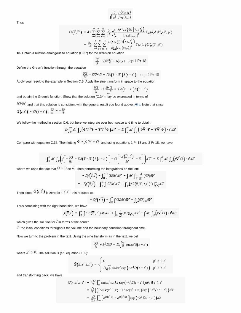
Thus
18. Obtain a relation analogous to equation (C.37) for the diffusion equation
Define the Green's function through the equation
Apply your result to the example in Section C.5. Apply the sine transform in space to the equation
and obtain the Green's function. Show that the solution (C.34) may be expressed in terms of
and that this solution is consistent with the general result you found above. Hint: Note that since
.
We follow the method in section C.6, but here we integrate over both space and time to obtain:
Compare with equation C.35. Then letting and using equations 1 Pr 18 and 2 Pr 18, we have
where we used the fact that on Then performing the integrations on the left:
Then since is zero for this reduces to:
Thus combining with the right hand side, we have
which gives the solution for in terms of the source
the initial conditions throughout the volume and the boundary condition throughout time.
Now we turn to the problem in the text. Using the sine transform as in the text, we get
where The solution is (c.f. equation C.32):
and transforming back, we have
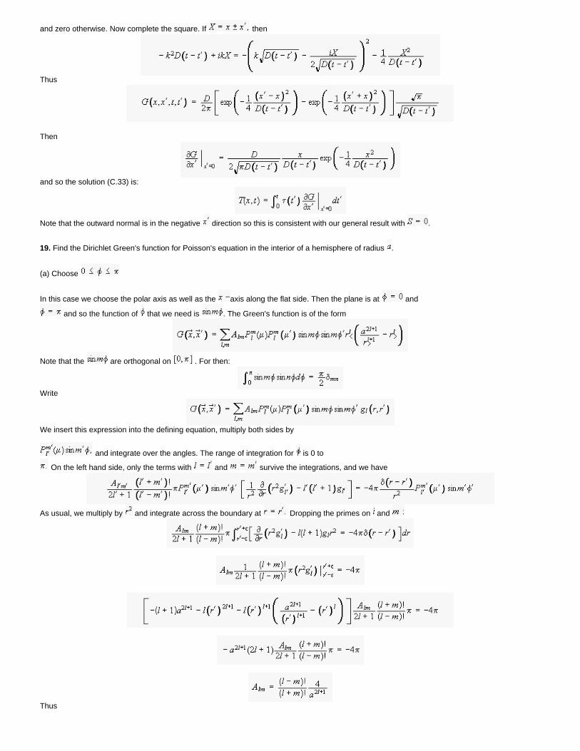
and zero otherwise. Now complete the square. If then
Thus
Then
and so the solution (C.33) is:
Note that the outward normal is in the negative direction so this is consistent with our general result with .
19. Find the Dirichlet Green's function for Poisson's equation in the interior of a hemisphere of radius .
(a) Choose
In this case we choose the polar axis as well as the axis along the flat side. Then the plane is at and
and so the function of that we need is . The Green's function is of the form
Note that the are orthogonal on . For then:
Write
We insert this expression into the defining equation, multiply both sides by
and integrate over the angles. The range of integration for is 0 to
On the left hand side, only the terms with and survive the integrations, and we have
As usual, we multiply by and integrate across the boundary at Dropping the primes on and
Thus
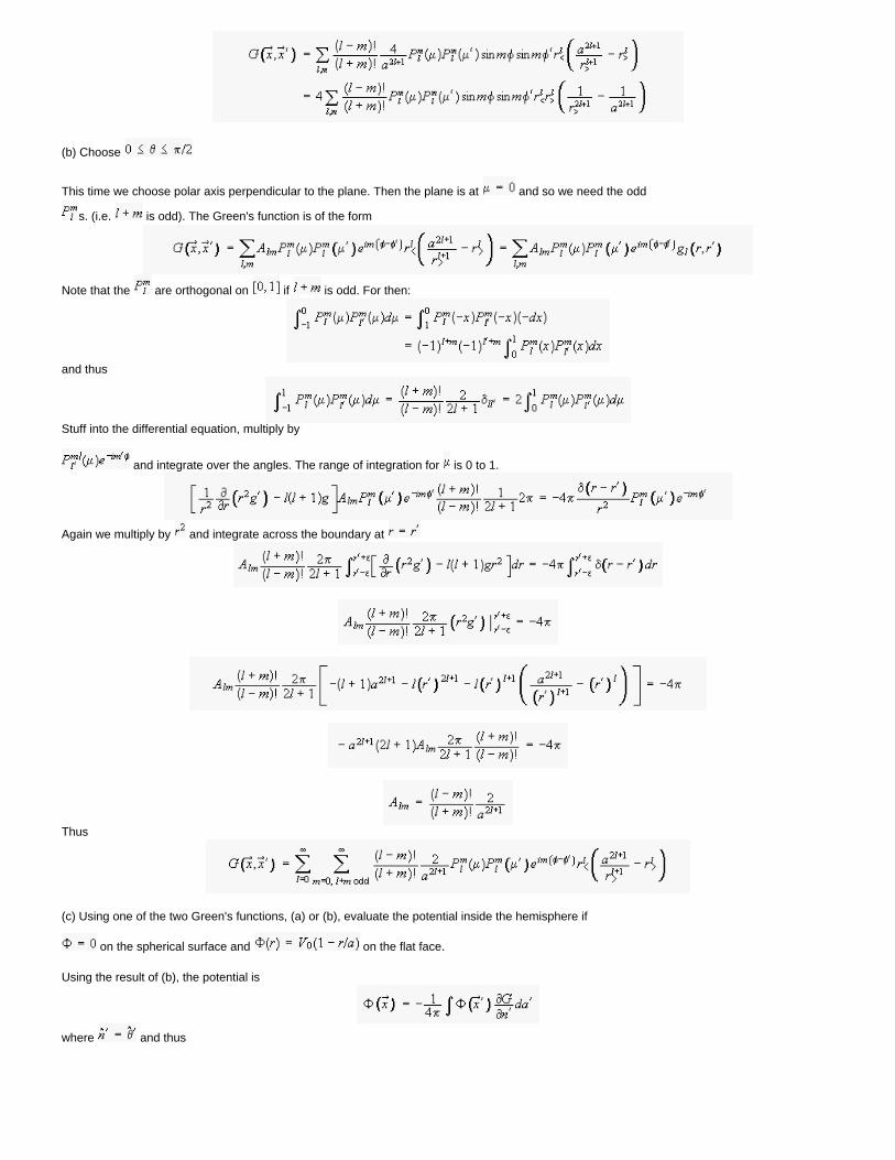
(b) Choose
This time we choose polar axis perpendicular to the plane. Then the plane is at and so we need the odd
s. (i.e. is odd). The Green's function is of the form
Note that the are orthogonal on if is odd. For then:
and thus
Stuff into the differential equation, multiply by
and integrate over the angles. The range of integration for is 0 to 1.
Again we multiply by and integrate across the boundary at
Thus
(c) Using one of the two Green's functions, (a) or (b), evaluate the potential inside the hemisphere if
on the spherical surface and on the flat face.
Using the result of (b), the potential is
where and thus
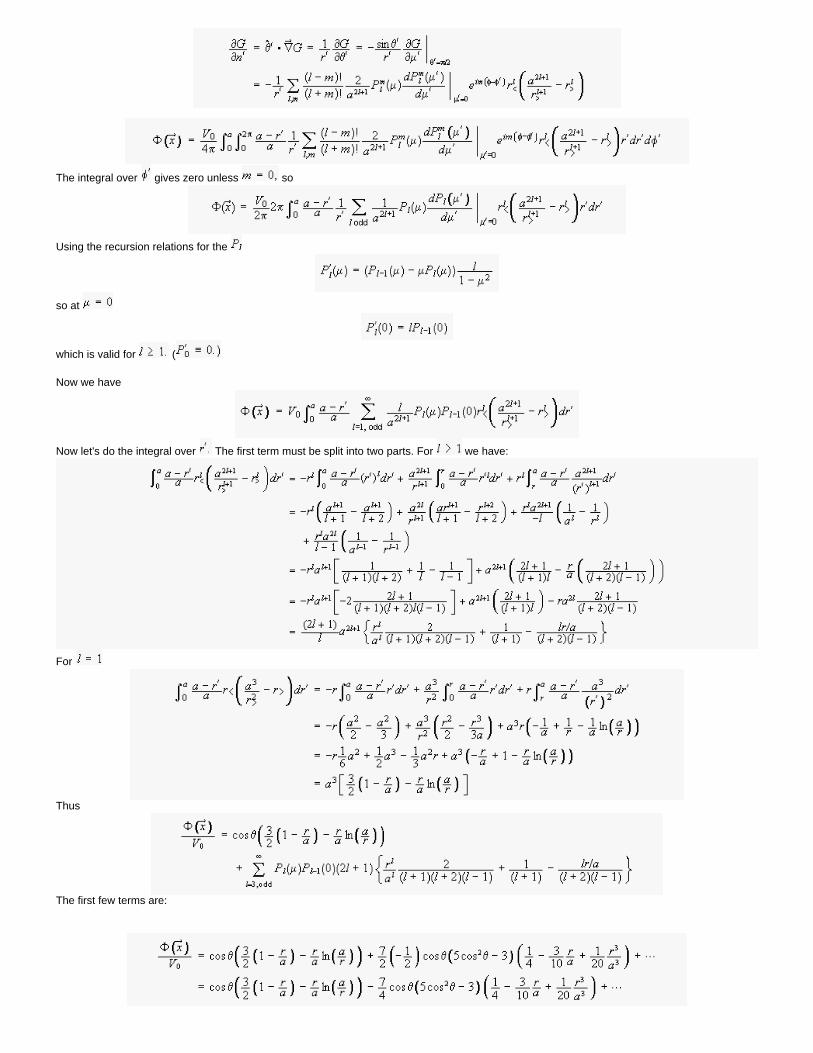
The integral over gives zero unless so
Using the recursion relations for the
so at
which is valid for (
Now we have
Now let's do the integral over The first term must be split into two parts. For we have:
For
Thus
The first few terms are:
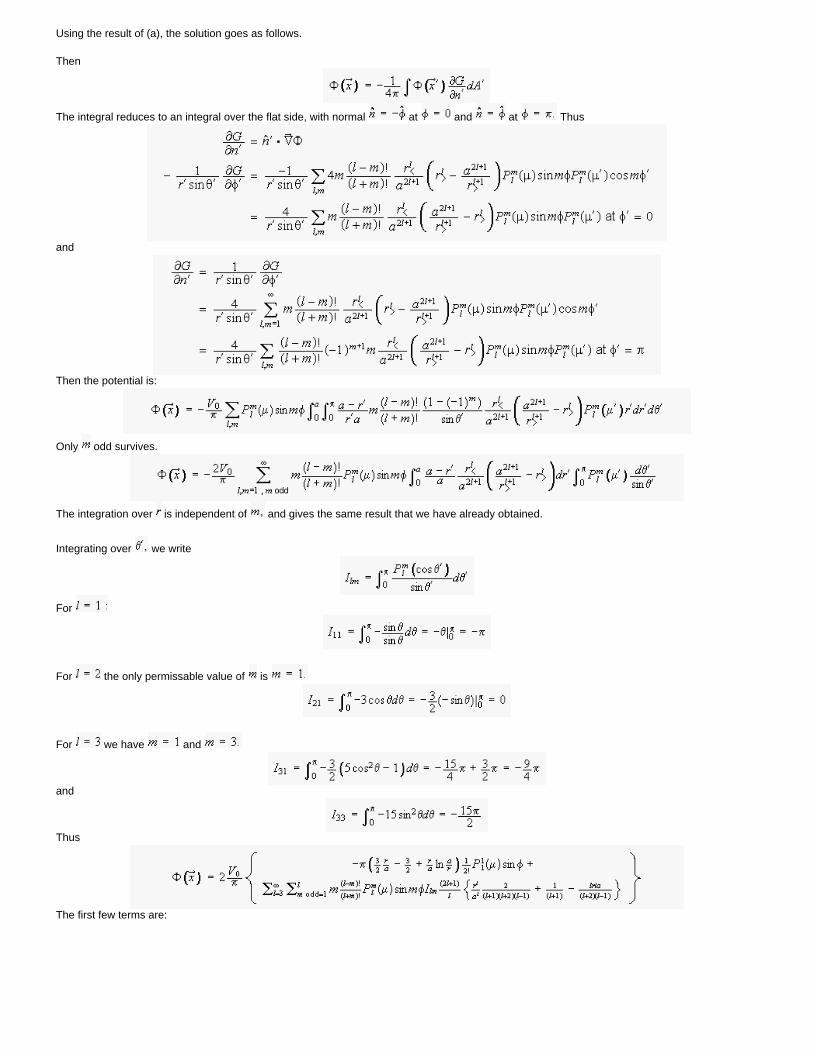
Using the result of (a), the solution goes as follows.
Then
The integral reduces to an integral over the flat side, with normal at and at Thus
and
Then the potential is:
Only odd survives.
The integration over is independent of and gives the same result that we have already obtained.
Integrating over we write
For
For the only permissable value of is
For we have and
and
Thus
The first few terms are:
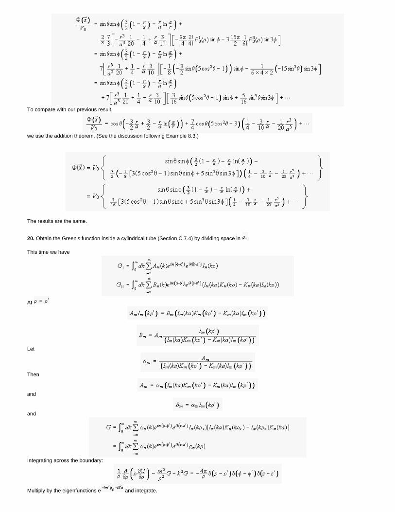
To compare with our previous result,
we use the addition theorem. (See the discussion following Example 8.3.)
The results are the same.
20. Obtain the Green's function inside a cylindrical tube (Section C.7.4) by dividing space in
This time we have
At
Let
Then
and
and
Integrating across the boundary:
Multiply by the eigenfunctions e and integrate.
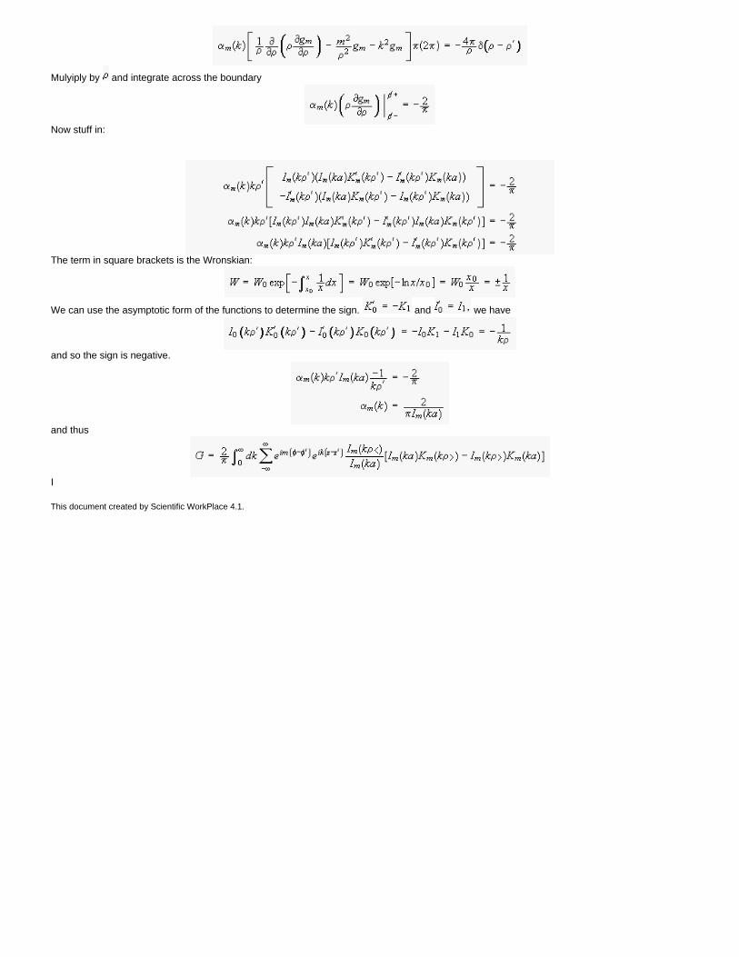
Mulyiply by and integrate across the boundary
Now stuff in:
The term in square brackets is the Wronskian:
We can use the asymptotic form of the functions to determine the sign. and we have
and so the sign is negative.
and thus
I
This document created by Scientific WorkPlace 4.1.
Optional Topic D: Approximate evaluation of integrals
1. Use the method of steepest descent to evaluate the asymptotic form of the Gamma function
First let
Next we write the integrand as an exponential in :
This is of the general form (D.2) with and Then
and
Thus
and
Then, applying the general result D.6, we have
This is Stirling's formula.
2. The modified Bessel function has an integral representation
Use the method of steepest descent to find the asymptotic form of as
The integral is of the standard form with
Thus Then
where we chose to put the deformed contour through the point , on the original contour. We also have
and
Thus
in agreement with Chapter 8 equation 8.105.
3. The Bessel function may be represented by an integral
where the contour is shown in the figure. Use the method of steepest descent or stationary phase, as appropriate, to derive the asymptotic form (8.83)
For complex the function is analytic and has both real and imaginary parts. So we use the method of steepest descent. First rewrite the integral in the standard form with
Then
Our contour runs through two of these points, at Then
Thus
If we deform the contour to go through the point along the line
(choosing in the expression for then goes from negative to positive and
so goes from negative to positive. At we have to choose
the sign, and again goes from negative to positive along the line
The contribution from each saddle is
and adding the two contributions, we get:
as required.
4. Expand the function in equation (D.7) in a Taylor series about the stationary point, and show that there is no contribution to the integral from the second (linear) term in the series, if
the expansion of the phase is truncated at the quadratic term, as in equation (D.8).
Equation (D.7) becomes:
The first term has already been evaluated in the text. Using the same methods, the second term is:
We may do the integral by the change of variable
to obtain
The integral over is zero since the integrand is an odd function. Thus the second term in the Taylor series does not contribute to the result.
5. The function has the integral expression
where the path of integration goes from to zero along a path in the lower-half plane that is the mirror image of the path in Figure 1. Verify the asymptotic form 8.85 for this function.
The solution follows the method in the text, with the following changes.
So and Thus the new path must pass through at an angle
. Before the difference has a negative real part on this path and
so is negative, as required.
and thus
as required.
6. An alternative integral expression for the Bessel functions is:
where
1. for use contour and
2. for use contour and
3. for use contour and
and the contours are shown in the figure. Evaluate the integrals for large values of and verify the asymptotic forms in Chapter 8.
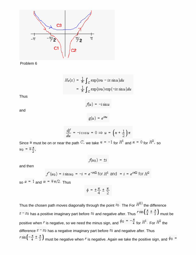
Problem 6
Thus
and
Since must be on or near the path we take for and for so
and then
so and Thus
Thus the chosen path moves diagonally through the point The For the difference
has a positive imaginary part before and negative after. Thus must be
positive when is negative, so we need the minus sign, and for For the
difference has a negative imaginary part before and negative after. Thus
must be negative when is negative. Again we take the positive sign, and
for . Finally, then:
and
These expressions agree with the results in Chapter 8.
For we have contributions from both saddles, and we obtain
as required.
7. The Airy integral
arises in the study of diffraction. The path of integration lies slightly above the real axis. Use the method of stationary phase to show that
The phase is
The stationary point is off the real axis, so we deform the path to go through one of these
points-- the one at We can do this because the integrand has no singularities between the two paths. (Recall that the path is above the real axis.) Then
and
The asymptotic form is (equation D.9):
as required.
8. The amplitude of a signal arriving from a distant source after propagation through a dispersive medium may be wriiten as a Fourier integral of the form:
where is the dispersion relation for the medium (see, e.g, Jackson Chapter 7). Use the method of stationary phase to show that the largest amplitude signal is contributed by
frequencies with group speed where is the distance from source to receiver,
and find an approximate expression for the amplitude at time .
The stationary phase condition is:
or the distance travelled by the signal at the group speed
By equation D.9, the amplitude is approximately:
where all derivatives are evaluated at and is a solution of the equation If there is more than one solution, then we must add the contributions from all the solutions.
Obtain an explicit form for the solution if and is a constant.
Thus
and the stationary phase condition is
or
There is no solution for as expected.
Evaluating at
Also
and
Putting it all together, we have
Thus the final result is:
This document created by Scientific WorkPlace 4.1.
Optional topic E: Calculus of variations 1. The speed of waves in a medium varies with as What is the path of a ray? This model describes the propagation of seismic waves through the Earth's outer layers. If the waves start at find the value of at which the waves return to the surface as a function of the initial slope of the ray
. Also determine the total time of travel for each ray. The time of travel is
Here the integrand is independent of and we may use equation (E.6).
or
Thus
Inserting the initial conditions ( at we have
Then
We integrate this expression to obtain
We may integrate immediately, to obtain:
and inserting the initial conditions,
Thus
The solution with that satisfies the condition at is
Equivalently,
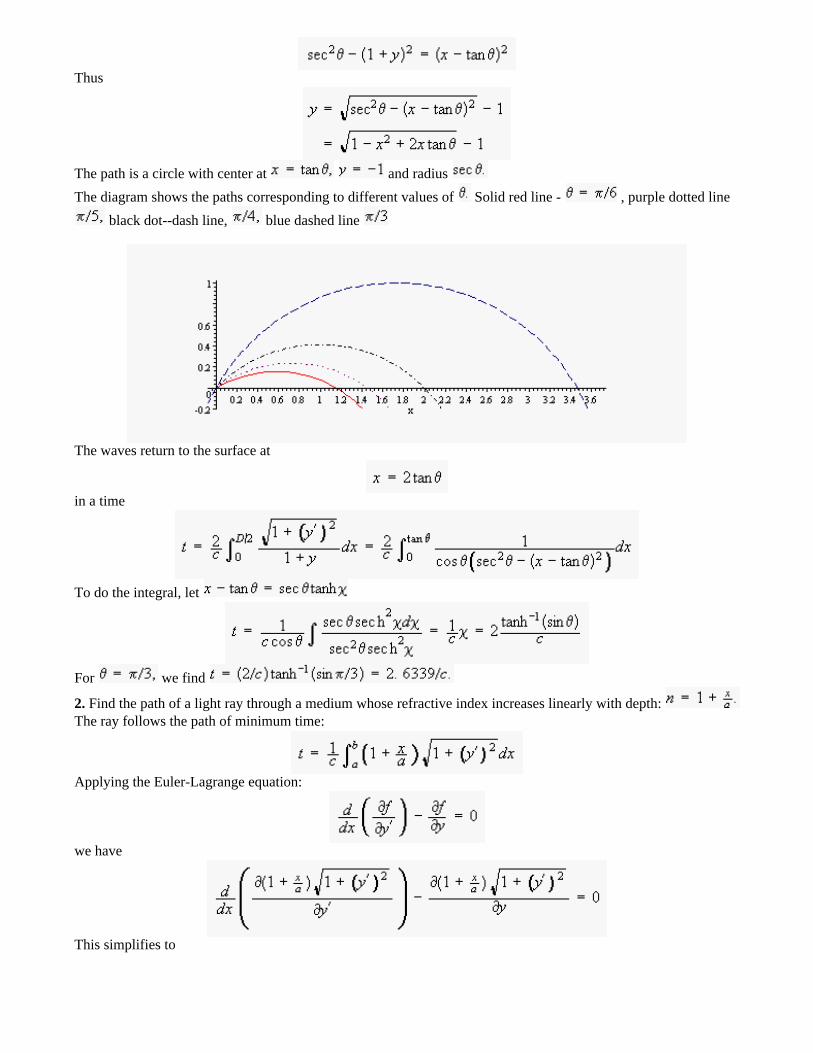
Thus
The path is a circle with center at and radius The diagram shows the paths corresponding to different values of Solid red line - , purple dotted line
black dot--dash line, blue dashed line
The waves return to the surface at
in a time
To do the integral, let
For we find
2. Find the path of a light ray through a medium whose refractive index increases linearly with depth: The ray follows the path of minimum time:
Applying the Euler-Lagrange equation:
we have
This simplifies to
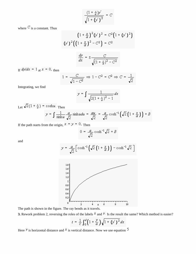
where is a constant. Thus
If at then
Integrating, we find
Let Then
If the path starts from the origin, Then
and
The path is shown in the figure. The ray bends as it travels. 3. Rework problem 2, reversing the roles of the labels and Is the result the same? Which method is easier?
Here is horizontal distance and is vertical distance. Now we use equation
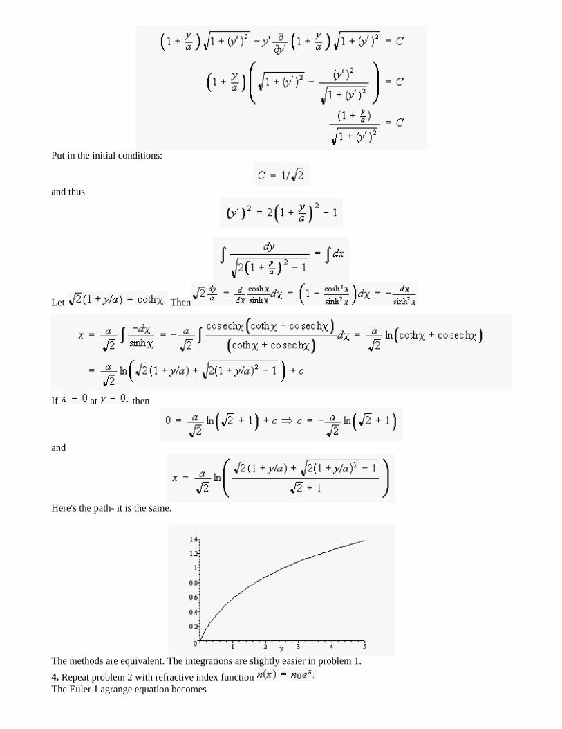
Put in the initial conditions:
and thus
Let Then
If at then
and
Here's the path- it is the same.
The methods are equivalent. The integrations are slightly easier in problem 1. 4. Repeat problem 2 with refractive index function The Euler-Lagrange equation becomes
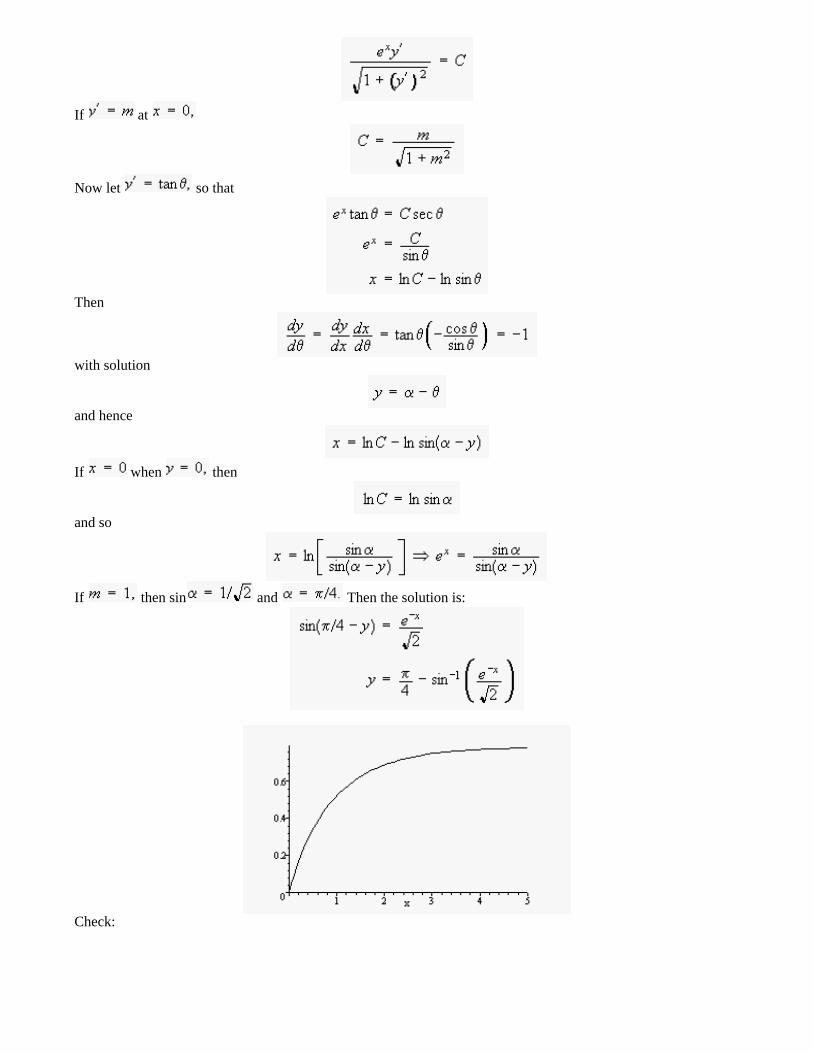
If at
Now let so that
Then
with solution
and hence
If when then
and so
If then sin and Then the solution is:
Check:
They agree. 5. The brachistochrone: A smooth wire runs between two fixed points and Find the shape of the wire such that a particle sliding without friction oin the wire reaches point in minimum time. Assume that the particle starts from point with speed Hint: set and obtain and as functions of Show that the coordinates of the two fixed points are sufficient to determine the intitial and final values of and the two integration constants. Determine an explicit solution in the case Plot the shape of the wire. We may find the speed of the particle at any time from conservation of energy.
Thus
and the time taken to go from to is
The problem is now in our standard form, and we may apply the Euler-Lagrange equation. Since the integrand does not depend explicitly on we may use equation (5):
Squaring both sides, we have:
The trick here is to let so that
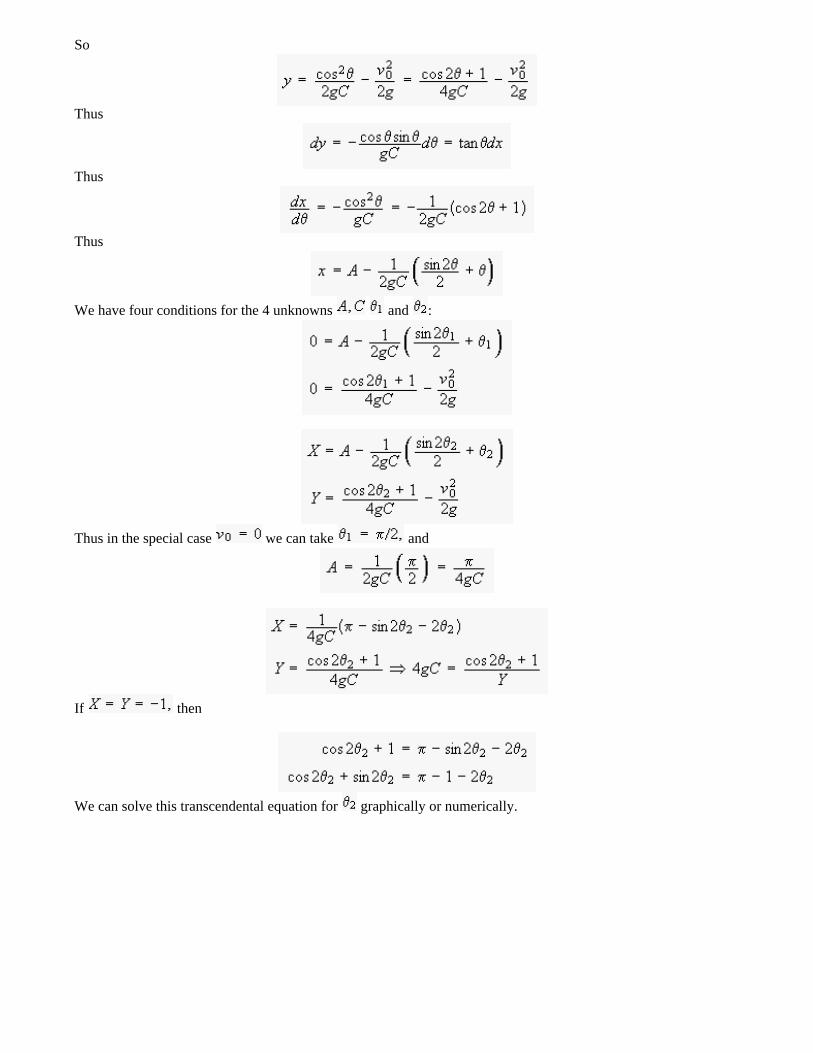
So
Thus
Thus
Thus
We have four conditions for the 4 unknowns and :
Thus in the special case we can take and
If then
We can solve this transcendental equation for graphically or numerically.
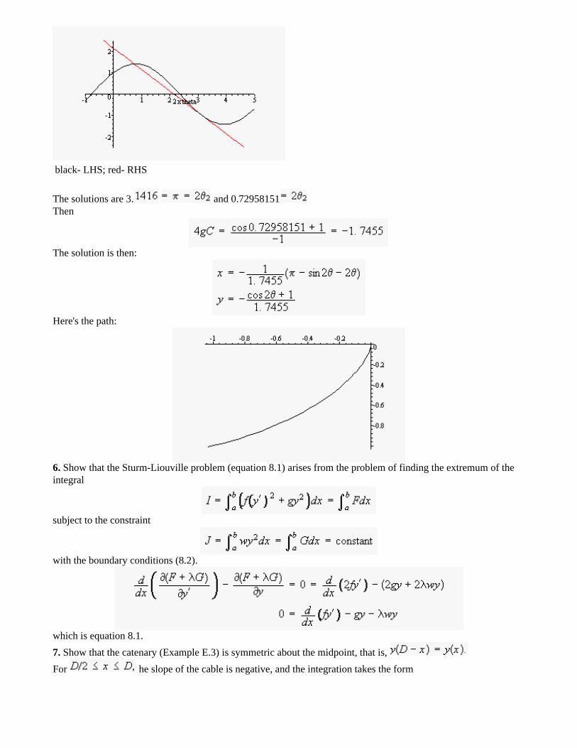
black- LHS; red- RHS
The solutions are 3. and 0.72958151 Then
The solution is then:
Here's the path:
6. Show that the Sturm-Liouville problem (equation 8.1) arises from the problem of finding the extremum of the integral
subject to the constraint
with the boundary conditions (8.2).
which is equation 8.1. 7. Show that the catenary (Example E.3) is symmetric about the midpoint, that is, For he slope of the cable is negative, and the integration takes the form
which gives the solution:
giving
as required. 8. Show that the curve that encloses the greatest area with a fixed perimeter is a circle. Let the curve be described by the function Then the area is
and the perimeter is
The integrands do not depend explicitly on so the appropriate equation is:
where
Thus
Let Then
So
and
and thus
Thus
This curve is a circle. This document created by Scientific WorkPlace 4.1.
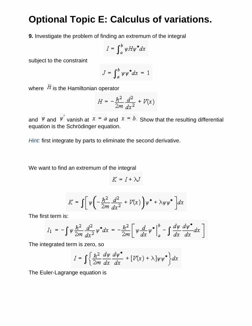
Optional Topic E: Calculus of variations.
9. Investigate the problem of finding an extremum of the integral
subject to the constraint
where is the Hamiltonian operator
and and vanish at and Show that the resulting differential equation is the Schrödinger equation.
Hint: first integrate by parts to eliminate the second derivative.
We want to find an extremum of the integral
The first term is:
The integrated term is zero, so
The Euler-Lagrange equation is
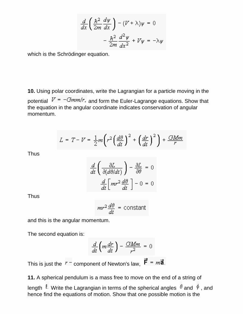
which is the Schrödinger equation.
10. Using polar coordinates, write the Lagrangian for a particle moving in the
potential and form the Euler-Lagrange equations. Show that the equation in the angular coordinate indicates conservation of angular momentum.
Thus
Thus
and this is the angular momentum.
The second equation is:
This is just the component of Newton's law,
11. A spherical pendulum is a mass free to move on the end of a string of
length Write the Lagrangian in terms of the spherical angles and , and hence find the equations of motion. Show that one possible motion is the
conical pendulum with constant What is the value of in this case?
The Largrange equations are''
Thus
and
With we retrieve the simple pendulum equations.
Now use the first equation to simplify the second:
If constant, then we have the conical pendulum with
and hence
12. Consider the one-dimensional motion of a particle with potential energy
that is independent of time. Show that The Euler Lagrange equations may be written in the form of equation (5). Give a physical interpretation of this equation.
Since does not depend explicitly on time, we may write the Euler-lagrange equations in the form:
Thus this equation states that the total (kinetic plus potential) energy is conserved in this system.
13. The Lagrangian for a vibrating string may be written
where is the displacement of the string, is the mass per unit length,
and is the tension. The first term in the integrand is the kinetic energy and the second is the potential energy. Determine the Euler-Lagrange equations for the system, and comment.
Here we have two independent variables, so:
and the equation is:
Setting the integrand to zero gives the wave equation for the string.
14. As an alternative approach to problem 13, we may expand the
displacement as a Fourier series in
Write the Lagragian as a function of the generalized coordinates and the
time What are the Euler-Lagrange equations now?
Thus
where we used the orthogonality of the sines and cosines to evaluate the
integrals. Now has one independent variable ( ) and infinitely many
independent variables Applying Hamilton's principle, the Euler-Lagrange equations take the form:
The solution for each must be of the form:
cf equation 4.28.
15. A volume is formed by rotating a curve defined for
around the axis. Given that the curve is symmetric about the
axis, , and show that the curve that gives the maximum volume for a given surface area is a circle and the
corresponding volume is a sphere..
The surface area is:
and the volume is
We can solve our problem by finding an extremum of The integrand,
does not depend on explicitly, thus equation 5
becomes:
If at then
Then
If when then Then
Now if at then
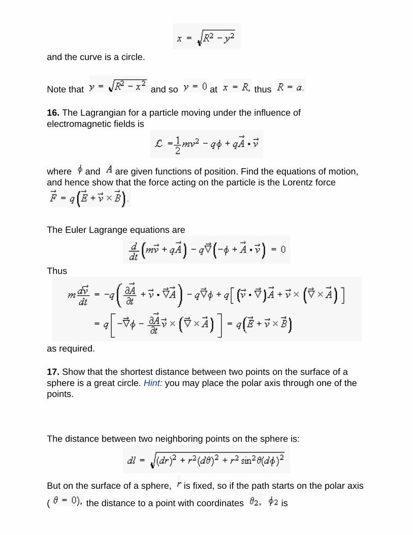
and the curve is a circle.
Note that and so at thus
16. The Lagrangian for a particle moving under the influence of electromagnetic fields is
where and are given functions of position. Find the equations of motion, and hence show that the force acting on the particle is the Lorentz force
The Euler Lagrange equations are
Thus
as required.
17. Show that the shortest distance between two points on the surface of a sphere is a great circle. Hint: you may place the polar axis through one of the points.
The distance between two neighboring points on the sphere is:
But on the surface of a sphere, is fixed, so if the path starts on the polar axis
( the distance to a point with coordinates is
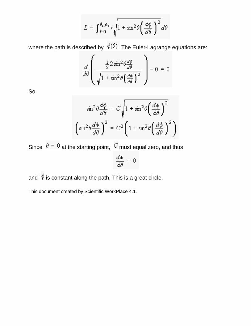
where the path is described by The Euler-Lagrange equations are:
So
Since at the starting point, must equal zero, and thus
and is constant along the path. This is a great circle.
This document created by Scientific WorkPlace 4.1.