mathematics of machine learning lecture notes - ocw.mit.edu · figure 1: the machine learning...

18.657: Mathematics of Machine Learning

Lecturer: Philippe Rigollet Lecture 1Scribe: Philippe Rigollet Sep. 9, 2015

1. WHAT IS MACHINE LEARNING (IN THIS COURSE)?

This course focuses on statistical learning theory, which roughly means understanding theamount of data required to achieve a certain prediction accuracy. To better understandwhat this means, we first focus on stating some differences between statistics and machinelearning since the two fields share common goals.

Indeed, both seem to try to use data to improve decisions. While these fields have evolvedin the same direction and currently share a lot of aspects, they were at the beginning quitedifferent. Statistics was around much before machine learning and statistics was alreadya fully developed scientific discipline by 1920, most notably thanks to the contributions ofR. Fisher, who popularized maximum likelihood estimation (MLE) as a systematic tool forstatistical inference. However, MLE requires essentially knowing the probability distributionfrom which the data is draw, up to some unknown parameter of interest. Often, the unknownparameter has a physical meaning and its estimation is key in better understanding somephenomena. Enabling MLE thus requires knowing a lot about the data generating process:this is known as modeling. Modeling can be driven by physics or prior knowledge of theproblem. In any case, it requires quite a bit of domain knowledge.

More recently (examples go back to the 1960’s) new types of datasets (demographics,social, medical,. . . ) have become available. However, modeling the data that they containis much more hazardous since we do not understand very well the input/output processthus requiring a distribution free approach. A typical example is image classification wherethe goal is to label an image simply from a digitalization of this image. Understandingwhat makes an image a cat or a dog for example is a very complicated process. However,for the classification task, one does not need to understand the labelling process but ratherto replicate it. In that sense, machine learning favors a blackbox approach (see Figure 1).

input X output Yblackbox y = f(x) + ε

input X output Y

Figure 1: The machine learning blackbox (left) where the goal is to replicate input/outputpairs from past observations, versus the statistical approach that opens the blackbox andmodels the relationship.

These differences between statistics and machine learning have receded over the lastcouple of decades. Indeed, on the one hand, statistics is more and more concerned withfinite sample analysis, model misspecification and computational considerations. On theother hand, probabilistic modeling is now inherent to machine learning. At the intersectionof the two fields, lies statistical learning theory, a field which is primarily concerned withsample complexity questions, some of which will be the focus of this class.

1

2. STATISTICAL LEARNING THEORY

2.1 Binary classification

A large part of this class will be devoted to one of the simplest problem of statistical learningtheory: binary classification (aka pattern recognition [DGL96]). In this problem, we observe(X1, Y1), . . . , (Xn, Yn) that are n independent random copies of (X,Y ) ∈ X ×0, 1. Denoteby PX,Y the joint distribution of (X,Y ). The so-called feature X lives in some abstractspace X (think IRd) and Y ∈ 0, 1 is called label. For example, X can be a collection ofgene expression levels measured on a patient and Y indicates if this person suffers fromobesity. The goal of binary classification is to build a rule to predict Y given X usingonly the data at hand. Such a rule is a function h : X → 0, 1 called a classifier. Someclassifiers are better than others and we will favor ones that have low classification errorR(h) = IP(h(X) = Y ). Let us make some important remarks.

Fist of all, since Y ∈ 0, 1 then Y has a Bernoulli distribution: so much for distributionfree assumptions! However, we will not make assumptions on the marginal distribution ofX or, what matters for prediction, the conditional distribution of Y given X. We write,Y |X ∼ Ber(η(X)), where η(X) = IP(Y = 1|X) = IE[Y |X] is called the regression functionof Y onto X.

Next, note that we did not write Y = η(X). Actually we have Y = η(X) + ε, whereε = Y −η(X) is a “noise” random variable that satisfies IE[ε|X] = 0. In particular, this noiseaccounts for the fact that X may not contain enough information to predict Y perfectly.This is clearly the case in our genomic example above: it not whether there is even anyinformation about obesity contained in a patient’s genotype. The noise vanishes if and onlyif η(x) ∈ 0, 1 for all x ∈ X . Figure 2.1 illustrates the case where there is no noise and thethe more realistic case where there is noise. When η(x) is close to .5, there is essentially noinformation about Y in X as the Y is determined essentially by a toss up. In this case, itis clear that even with an infinite amount of data to learn from, we cannot predict Y wellsince there is nothing to learn. We will see what the effect of the noise also appears in thesample complexity.

6

Figure 2: The thick black curve corresponds to the noiseless case where Y = η(X) ∈ 0, 1and the thin red curve corresponds to the more realistic case where η ∈ [0, 1]. In the lattercase, even full knowledge of η does not guarantee a perfect prediction of Y .

In the presence of noise, since we cannot predict Y accurately, we cannot drive theclassification error R(h) to zero, regardless of what classifier h we use. What is the smallestvalue that can be achieved? As a thought experiment, assume to begin with that we have all

x

η(x)

1

.5

2

the information that we may ever hope to get, namely we know the regression function η(·).For a given X to classify, if η(X) = 1/2 we may just toss a coin to decide our predictionand discard X since it contains no information about Y . However, if η(X) = 1/2, we havean edge over random guessing: if η(X) > 1/2, it means that IP(Y = 1|X) > IP(Y = 0|X)or, in words, that 1 is more likely to be the correct label. We will see that the classifierh∗(X) = 1I(η(X) > 1/2) (called Bayes classifier) is actually the best possible classifier inthe sense that

R(h∗) = inf R(h) ,h(·)

where the infimum is taken over all classifiers, i.e. functions from X to 0, 1. Note thatunless η(x) ∈ 0, 1 for all x ∈ X (noiseless case), we have R(h∗) = 0. However, we canalways look at the excess risk E(h) of a classifier h defined by

E(h) = R(h)−R(h∗) ≥ 0 .

In particular, we can hope to drive the excess risk to zero with enough observations bymimicking h∗ accurately.

2.2 Empirical risk

The Bayes classifier h∗, while optimal, presents a major drawback: we cannot compute itbecause we do not know the regression function η. Instead, we have access to the data(X1, Y1), . . . , (Xn, Yn), which contains some (but not all) information about η and thus h∗.In order to mimic the properties of h∗ recall that it minimizes R(h) over all h. But thefunction R(·) is unknown since it depends on the unknown distribution PX,Y of (X,Y ). We

ˆestimate it by the empirical classification error, or simply empirical risk Rn(·) defined forany classifier h by

n1

Rn(h) =∑

1I(h(Xi) = Yi) .n

i=1

ˆ ˆSince IE[1I(h(Xi) = Yi)] = IP(h(Xi) = Yi) = R(h), we have IE[Rn(h)] = R(h) so Rn(h) isan unbiased estimator of R(h). Moreover, for any h, by the law of large numbers, we haveˆ ˆRn(h) → R(h) as n → ∞, almost surely. This indicates that if n is large enough, Rn(h)should be close to R(h).

As a result, in order to mimic the performance of h∗, let us use the empirical riskˆ ˆminimizer (ERM) h defined to minimize Rn(h) over all classifiers h. This is an easy enough

ˆ ˆtask: define h such h(Xi) = Yi for all i = 1, . . . , n and h(x) = 0 if x ∈/ X1, . . . ,Xn. Weˆ ˆhave Rn(h) = 0, which is clearly minimal. The problem with this classifier is obvious: it

does not generalize outside the data. Rather, it predicts the label 0 for any x that is not inˆ ˆthe data. We could have predicted 1 or any combination of 0 and 1 and still get Rn(h) = 0.

ˆIn particular it is unlikely that IE[R(h)] will be small.

6

6

6

6 6

3

Important Remark: Recall that R(h) = IP(h(X) 6= Y ).ˆ ˆ Îf h(·) = h((X1, Y1), . . . , (Xn, Yn) ; ·) is constructed from the data, R(h) denotes

the conditional probability

ˆ ˆR(h) = IP(h(X) 6= Y |(X1, Y1), . . . , (Xn, Yn)) .

ˆ ˆrather than IP(h(X) 6= Y ). As a result R(h) is a random variable since it depends on therandomness of the data (X1, Y1), . . . , (Xn, Yn). One way to view this is to observe that

ˆwe compute the deterministic function R(·) and then plug in the random classifier h.

This problem is inherent to any method if we are not willing to make any assumptionon the distribution of (X,Y ) (again, so much for distribution freeness!). This can actuallybe formalized in theorems, known as no-free-lunch theorems.

Theorem: ˆFor any integer n ≥ 1, any classifier h built from (X1, Y1), . . . , (Xn, Yn) andany ε > 0, there exists a distribution PX,Y for (X,Y ) such that R(h∗) = 0 and

ÎER(hn) ≥ 1/2 − ε .

To be fair, note that here the distribution of the pair (X,Y ) is allowed to depend onn which is cheating a bit but there are weaker versions of the no-free-lunch theorem thatessentially imply that it is impossible to learn without further assumptions. One suchtheorem is the following.

Theorem: ˆFor any classifier h built from (X1, Y1), . . . , (Xn, Yn) and any sequenceann > 0 that converges to 0, there exists a distribution PX,Y for (X,Y ) such thatR(h∗) = 0 and

ÎER(hn) ≥ an , for all n ≥ 1

In the above theorem, the distribution of (X,Y ) is allowed to depend on the whole sequenceann > 0 but not on a specific n. The above result implies that the convergence to zero ofthe classification error may be arbitrarily slow.

2.3 Generative vs discriminative approaches

Both theorems above imply that we need to restrict the distribution PX,Y of (X,Y ). Butisn’t that exactly what statistical modeling is? The is answer is not so clear depending onhow we perform this restriction. There are essentially two schools: generative which is thestatistical modeling approach and discriminative which is the machine learning approach.

Generative: This approach consists in restricting the set of candidate distributions PX,Y .This is what is done in discriminant analysis1where it is assumed that the condition dis-

1Amusingly, the generative approach is called discriminant analysis but don’t let the terminology fool

you.

4

tributions of X given Y (there are only two of them: one for Y = 0 and one for Y = 1) areGaussians on X = IRd (see for example [HTF09] for an overview of this approach).

Discriminative: This is the machine learning approach. Rather than making assumptionsdirectly on the distribution, one makes assumptions on what classifiers are likely to performcorrectly. In turn, this allows to eliminate classifiers such as the one described above andthat does not generalize well.

While it is important to understand both, we will focus on the discriminative approachin this class. Specifically we are going to assume that we are given a class H of classifierssuch that R(h) is small for some h ∈ H.

2.4 Estimation vs. approximation

Assume that we are given a class H in which we expect to find a classifier that performs well.This class may be constructed from domain knowledge or simply computational convenience.

ˆWe will see some examples in the class. For any candidate classifier hn built from the data,we can decompose its excess risk as follows:

ˆ ˆ ˆE(hn) = R(hn)−R(h∗) = R(hn)− inf R(h)+ inf R(h)−R(h∗) .h∈H h∈H

︸

estimat

︷

io

︷

n error

︸︸

approxim

︷

a

︷

tion error

︸

On the one hand, estimation error accounts for the fact that we only have a finiteamount of observations and thus a partial knowledge of the distribution PX,Y . Hopefullywe can drive this error to zero as n → ∞. But we already know from the no-free-lunchtheorem that this will not happen if H is the set of all classifiers. Therefore, we need totake H small enough. On the other hand, if H is too small, it is unlikely that we willfind classifier with performance close to that of h∗. A tradeoff between estimation andapproximation can be made by letting H = Hn grow (but not too fast) with n.

For now, assume that H is fixed. The goal of statistical learning theory is to understandhow the estimation error drops to zero as a function not only of n but also of H. For thefirst argument, we will use concentration inequalities such as Hoeffding’s and Bernstein’sinequalities that allow us to control how close the empirical risk is to the classification errorby bounding the random variable

∣ n1∣ ∑

1I(h(X (h∣ i) = Yi)− IP (X) = Y )∣

n∣

i=1

∣

with high probability. More generally we will be interested in results that allow to quantifyhow close the average of independent and identically distributed (i.i.d) random variables isto their common expected value.

ˆ ˆ ˆIndeed, since by definition, we have Rn(h) ≤ Rn(h) for all h ∈ H, the estimation error¯can be controlled as follows. Define h ∈ H to be any classifier that minimizes R(·) over H

(assuming that such a classifier exist).

ˆ ˆ ¯R(hn)− inf R(h) = R(hn)−R(h)h∈H

ˆ ˆ ˆ ¯ ˆ ˆ ¯ ¯= Rn(hn)−Rn(h)+R(hn)− Rn(h ) + Rn n(h)−R(h)︸

≤

︷︷

0

︸

≤∣∣ ˆ ˆ ˆ ˆ ¯ ¯Rn(hn)−R(hn)

∣∣+

∣∣Rn(h)−R(h)

∣∣ .

6 6

5

¯ ˆ ¯ ¯Since h is deterministic, we can use a concentration inequality to control∣∣Rn(h) − R(h)

∣∣.

However,n

1ˆ ˆ ˆRn(hn) =∑

1I(hn(Xi) = Yi)n

i=1

is not ˆthe average of independent random variables since hn depends in a complicatedmanner on all of the pairs (Xi, Yi), i = 1, . . . , n. To overcome this limitation, we often use

ˆa blunt, but surprisingly accurate tool: we “sup out” hn,

∣∣ ˆ ˆ ˆ ˆ ˆ ˆRn(hn)−R(hn)

∣∣ ≤ sup

∣

h∈

∣Rn(hn)−R(hn)∣

H

∣ .

Controlling this supremum falls in the scope of suprema of empirical processes that we willstudy in quite a bit of detail. Clearly the supremum is smaller as H is smaller but H shouldbe kept large enough to have good approximation properties. This is the tradeoff betweenapproximation and estimation. It is also know in statistics as the bias-variance tradeoff.

6

6


Lecturer: Philippe Rigollet Lecture 2Scribe: Jonathan Weed Sep. 14, 2015

Part I

Statistical Learning Theory

1. BINARY CLASSIFICATION

In the last lecture, we looked broadly at the problems that machine learning seeks to solveand the techniques we will cover in this course. Today, we will focus on one such problem,binary classification, and review some important notions that will be foundational for therest of the course.

Our present focus on the problem of binary classification is justified because both binaryclassification encompasses much of what we want to accomplish in practice and because theresponse variables in the binary classification problem are bounded. (We will see a veryimportant application of this fact below.) It also happens that there are some nasty surprisesin non-binary classification, which we avoid by focusing on the binary case here.

1.1 Bayes Classifier

Recall the setup of binary classification: we observe a sequence (X1, Y1), . . . , (Xn, Yn) of nindependent draws from a joint distribution PX,Y . The variable Y (called the label) takesvalues in 0, 1, and the variable X takes values in some space X representing “features” ofthe problem. We can of course speak of the marginal distribution PX of X alone; moreover,since Y is supported on 0, 1, the conditional random variable Y |X is distributed accordingto a Bernoulli distribution. We write Y |X ∼ Bernoulli(η(X)), where

η(X) = IP(Y = 1|X) = IE[Y |X].

(The function η is called the regression function.)We begin by defining an optimal classifier called the Bayes classifier. Intuitively, the

Bayes classifier is the classifier that “knows” η—it is the classifier we would use if we hadperfect access to the distribution Y |X.

Definition: The Bayes classifier of X given Y , denoted h∗, is the function defined by therule

(h

1 if η x) > 1/2∗(x) =0 if η(x) ≤ 1/2.

In other words, h∗(X) = 1 whenever IP(Y = 1|X) > IP(Y = 0|X).Our measure of performance for any classifier h (that is, any function mapping X to

0, 1) will be the classification error : R(h) = IP(Y = h(X)). The Bayes risk is the valueR∗ = R(h∗) of the classification error associated with the Bayes classifier. The followingtheorem establishes that the Bayes classifier is optimal with respect to this metric.

6

7

Theorem: For any classifier h, the following identity holds:

R(h)−R(h∗) =

∫|2η(x)− 1|Px(dx) = IEX [|2η(X)− 1|1(h(X) = h∗(X))] (1.1)

h=h∗

Where h = h∗ is the (measurable) set x ∈ X | h(x) = h∗(x).In particular, since the integrand is nonnegative, the classification error R∗ of the

Bayes classifier is the minimizer of R(h) over all classifiers h.Moreover,

1R(h∗) = IE[min(η(X), 1− η(X))] ≤ . (1.2)

2

Proof. We begin by proving Equation (1.2). The definition of R(h) implies

R(h) = IP(Y = h(X)) = IP(Y = 1, h(X) = 0) + IP(Y = 0, h(X) = 1),

where the second equality follows since the two events are disjoint. By conditioning on Xand using the tower law, this last quantity is equal to

IE[IE[1(Y = 1, h(X) = 0)|X]] + IE[IE[1(Y = 0, h(X) = 1)|X]]

Now, h(X) is measurable with respect to X, so we can factor it out to yield

IE[1(h(X) = 0)η(X) + 1(h(X) = 1)(1− η(X))]], (1.3)

where we have replaced IE[Y |X] by η(X).In particular, if h = h∗, then Equation 1.3 becomes

IE[1(η(X) ≤ 1/2)η(X) + 1(η(x) > 1/2)(1− η(X))].

But η(X) ≤ 1/2 implies η(X) ≤ 1− η(X) and conversely, so we finally obtain

R(h∗) = IE[1(η(X) ≤ 1/2)η(X) + 1(η(x) > 1/2)(1− η(X))]

= IE[(1(η(X) ≤ 1/2) + 1(η(x) > 1/2)) min(η(X), 1− η(X))]

= IE[min(η(X), 1− η(X))],

as claimed. Since min(η(X), 1− η(X)) ≤ 1/2, its expectation is also certainly at most 1/2as well.

Now, given an arbitrary h, applying Equation 1.3 to both h and h∗ yields

R(h)−R(h∗) = IE[1(h(X) = 0)η(X) + 1(h(X) = 1)(1− η(X))]

−1(h∗(X) = 0)η(X) + 1(h∗(X) = 1)(1− η(X))]],

which is equal to

IE[(1(h(X) = 0)− 1(h∗(X) = 0))η(X) + (1(h(X) = 1)− 1(h∗(X) = 1))(1− η(X))].

Since h(X) takes only the values 0 and 1, the second term can be rewritten as −(1(h(X) =0)− 1(h∗(X) = 0)). Factoring yields

IE[(2η(X)− 1)(1(h(X) = 0)− 1(h∗(X) = 0))].

66

6

6

8

The term 1(h(X) = 0)− 1(h∗(X) = 0) is equal to −1, 0, or 1 depending on whether hand h∗ agree. When h(X) = h∗(X), it is zero. When h(X) = h∗(X), it equals 1 wheneverh∗(X) = 0 and −1 otherwise. Applying the definition of the Bayes classifier, we obtain

IE[(2η(X)− 1)1(h(X) = h∗(X)) sign(η − 1/2)] = IE[|2η(X)− 1|1(h(X) = h∗(X))],

as desired.

We make several remarks. First, the quantity R(h) − R(h∗) in the statement of thetheorem above is called the excess risk of h and denoted E(h). (“Excess,” that is, abovethe Bayes classifier.) The theorem implies that E(h) ≥ 0.

Second, the risk of the Bayes classifier R∗ equals 1/2 if and only if η(X) = 1/2 almostsurely. This maximal risk for the Bayes classifier occurs precisely when Y “contains noinformation” about the feature variable X. Equation (1.1) makes clear that the excess riskweighs the discrepancy between h and h∗ according to how far η is from 1/2. When η isclose to 1/2, no classifier can perform well and the excess risk is low. When η is far from1/2, the Bayes classifier performs well and we penalize classifiers that fail to do so moreheavily.

As noted last time, linear discriminant analysis attacks binary classification by puttingsome model on the data. One way to achieve this is to impose some distributional assump-tions on the conditional distributions X|Y = 0 and X|Y = 1.

We can reformulate the Bayes classifier in these terms by applying Bayes’ rule:

IP(X = x Y = 1)IP(Y = 1)η(x) = IP(Y = 1

||X = x) = .IP(X = x|Y = 1)IP(Y = 1) + IP(X = x|Y = 0)IP(Y = 0)

(In general, when PX is a continuous distribution, we should consider infinitesimal proba-bilities IP(X ∈ dx).)

Assume that X|Y = 0 and X|Y = 1 have densities p0 and p1, and IP(Y = 1) = π issome constant reflecting the underlying tendency of the label Y . (Typically, we imaginethat π is close to 1/2, but that need not be the case: in many applications, such as anomalydetection, Y = 1 is a rare event.) Then h∗(X) = 1 whenever η(X) ≥ 1/2, or, equivalently,whenever

p1(x) 1− π.

p0(x)≥

π

When π = 1/2, this rule amounts to reporting 1 or 0 by comparing the densities p1and p0. For instance, in Figure 1, if π = 1/2 then the Bayes classifier reports 1 wheneverp1 ≥ p0, i.e., to the right of the dotted line, and 0 otherwise.

On the other hand, when π is far from 1/2, the Bayes classifier is weighed towards theunderlying bias of the label variable Y .

1.2 Empirical Risk Minimization

The above considerations are all probabilistic, in the sense that they discuss properties ofsome underlying probability distribution. The statistician does not have access to the trueprobability distribution PX,Y ; she only has access to i.i.d. samples (X1, Y1), . . . , (Xn, Yn).We consider now this statistical perspective. Note that the underlying distribution PX,Ystill appears explicitly in what follows, since that is how we measure our performance: wejudge the classifiers we produced on future i.i.d. draws from PX,Y .

6

6 6

9

Figure 1: The Bayes classifier when π = 1/2.

Given data Dn = ˆ(X1, Y1), . . . , (Xn, Yn), we build a classifier hn(X), which is randomin two senses: it is a function of a random variable X and also depends implicitly on the

ˆrandom data Dn. As above, we judge a classifier according to the quantity E(hn). This isa random variable: though we have integrated out X, the excess risk still depends on thedata Dn. We therefore will consider bounds both on its expected value and bounds that

ˆhold in high probability. In any case, the bound E(hn) ≥ 0 always holds. (This inequalitydoes not merely hold “almost surely,” since we proved that R(h) ≥ R(h∗) uniformly overall choices of classifier h.)

Last time, we proposed two different philosophical approaches to this problem. Inparticular, generative approaches make distributional assumptions about the data, attemptto learn parameters of these distributions, and then plug the resulting values into the model.The discriminative approach—the one taken in machine learning—will be described in greatdetail over the course of this semester. However, there is some middle ground, which is worthmentioning briefly. This middle ground avoids making explicit distributional assumptionsabout X while maintaining some of the flavor of the generative model.

The central insight of this middle approach is the following: since by definition h∗(x) =ˆ1(η(X) > 1/2), we estimate η by some ηn and thereby produce the estimator hn =

1(ηn(X) > 1/2). The result is called a plug-in estimator.Of course, achieving good performance with a plug-in estimator requires some assump-

tions. (No-free-lunch theorems imply that we can’t avoid making an assumption some-where!) One possible assumption is that η(X) is smooth; in that case, there are manynonparamteric regression techniques available (Nadaraya-Watson kernel regression, waveletbases, etc.).

We could also assume that η(X) is a function of a particular form. Since η(X) is onlysupported on [0, 1], standard linear models are generally inapplicable; rather, by applyingthe logit transform we obtain logistic regression, which assumes that η satisfies an identityof the form

log

(η(X)

1− η(X)

)= θTX.

Plug-in estimators are called “semi-paramteric” since they avoid making any assumptionsabout the distribution of X. These estimators are widely used because they perform fairlywell in practice and are very easy to compute. Nevertheless, they will not be our focus here.

In what follows, we focus here on the discriminative framework and empirical risk min-imization. Our benchmark continues to be the risk function R(h) = IE1(Y = h(X)), which6

10

is clearly not computable based on the data alone; however, we can attempt to use a naıvestatistical “hammer” and replace the expectation with an average.

Definition: The empirical risk of a classifier h is given by

n1

Rn(h) =∑

1(Yi = h(Xi)).ni=1

Minimizing the empirical risk over the family of all classifiers is useless, since we canalways minimize the empirical risk by mimicking the data and classifying arbitrarily other-wise. We therefore limit our attention to classifiers in a certain family H.

ˆDefinition: The Empirical Risk Minimizer (ERM) over H is any element1 herm of the setˆargminh Rn(h).∈H

In order for our results to be meaningful, the class H must be much smaller than theˆspace of all classifiers. On the other hand, we also hope that the risk of herm will be close

to the Bayes risk, but that is unlikely if H is too small. The next section will give us toolsfor quantifying this tradeoff.

1.3 Oracle Inequalities

An oracle is a mythical classifier, one that is impossible to construct from data alone but¯whose performance we nevertheless hope to mimic. Specifically, given H we define h to be

an element of argminh R(h)—a classifier in∈H H that minimizes the true risk. Of course,¯we cannot determine h, but we can hope to prove a bound of the form

ˆR(h) ≤ ¯R(h) + something small. (1.4)

¯Since h is the best minimizer in H given perfect knowledge of the distribution, a bound ofˆthe form given in Equation 1.4 would imply that h has performance that is almost best-in-

class. We can also apply such an inequality in the so-called improper learning framework,ˆwhere we allow h to lie in a slightly larger class H′

ˆ⊃ H; in that case, we still get nontrivial

¯guarantees on the performance of h if we know how to control R(h)There is a natural tradeoff between the two terms on the right-hand side of Equation 1.4.

When H ¯is small, we expect the performance of the oracle h to suffer, but we may hope¯to approximate h quite closely. (Indeed, at the limit where H is a single function, the

“something small” in Equation 1.4 is equal to zero.) On the other hand, as H grows theoracle will become more powerful but approximating it becomes more statistically difficult.(In other words, we need a larger sample size to achieve the same measure of performance.)

ˆSince R(h) is a random variable, we ultimately want to prove a bound in expectationor tail bound of the form

ˆIP(R(h) ≤ ¯R(h) + ∆n,δ(H)) ≥ 1− δ,

where ∆n,δ(H) is some explicit term depending on our sample size and our desired level ofconfidence.

1In fact, even an approximate solution will do: our bounds will still hold whenever we produce a classifierˆ ˆ ˆh satisfying Rn(h) ≤ infh R∈H n(h) + ε.

6

11

In the end, we should recall that

E ˆ ˆ − ∗ ˆ − ¯ ¯(h) = R(h) R(h ) = (R(h) R(h)) + (R(h)−R(h∗)).

The second term in the above equation is the approximation error, which is unavoidableonce we fix the class H. Oracle inequalities give a means of bounding the first term, thestochastic error.

1.4 Hoeffding’s Theorem

Our primary building block is the following important result, which allows us to understandhow closely the average of random variables matches their expectation.

Theorem (Hoeffding’s Theorem): Let X1, . . . , Xn be n independent random vari-ables such that Xi ∈ [0, 1] almost surely.

Then for any t > 0,

IP

(∣∣ n1 ∑

Xi IEXini=1

−∣∣∣>

)∣ ∣∣ 2t ≤ 2e−2nt .

In other words, deviations from

∣the mean deca

∣y exponentially fast in n and t.

Proof. Define centered random variables Zi = Xi − IEXi. It suffices to show that(1 ∑ )

≤ −2nt2IP Zi > t e ,n

since the lower tail bound follows analogously. (Exercise!)We apply Chernoff bounds. Since the exponential function is an order-preserving bijec-

tion, we have for any s > 0

IP

(1 ∑

Z stni > t

)= IP

(exp

(s∑

Z stn s Zii ]

n

)> e

)≤ e− IE[e

∑(Markov)

= e−stn IE[esZi ], (1.5)

where in the last equality we have used the independence of the

∏Zi.

We therefore need to control the term IE[esZi ], known as the moment-generating func-tion of Zi. If the Zi were normally distributed, we could compute the moment-generatingfunction analytically. The following lemma establishes that we can do something similarwhen the Zi are bounded.

Lemma (Hoeffding’s Lemma): If Z ∈ [a, b] almost surely and IEZ = 0, then

2 2

≤s (b−a)

IEesZ e 8 .

Proof of Lemma. Consider the log-moment generating function ψ(s) = log IE[esZ ], and notethat it suffices to show that ψ(s) ≤ s2(b − a)2/8. We will investigate ψ by computing the

12

first several terms of its Taylor expansion. Standard regularity conditions imply that wecan interchange the order of differentiation and integration to obtain

IE[ZesZ ]ψ′(s) = ,

IE[esZ ]2

IE[Z2esZ ]IE[esZ ] IE[ZesZ ]2 esZ esZψ′′(s) =

−= IE

[Z2

]−(

IE ZIE[esZ ]2 IE[esZ ]

[IE[esZ ]

]).

Since esZsZ integrates to 1, we can interpret ψ′′(s) as the variance of Z under the probability

IE[e ]

measure dF = esZsZ dIE. We obtain

IE[e ]

ψ′′(s) = varF(Z) = varF

(a+ b

Z −2

),

since the variance is unaffected under shifts. But |Z − a+b2 | ≤

b−a almost surely since2Z ∈ [a, b] almost surely, so

varF

(+ b

Z −2

)≤ F

[( 2a a+ bZ −

2

) ](b− a)2≤ .

4

Finally, the fundamental theorem of calculus yields

s u s2(b a)2ψ(s) =

∫(u du

0

∫ψ′′ )

−.

0≤

8

This concludes the proof of the Lemma.

Applying Hoeffding’s Lemma to Equation (1.5), we obtain

IP

(1 ∑ 2

Z > t

)≤ e−stn

∏es

2/8 = ens /8 stni

− ,n

for any s > 0. Plugging in s = 4t > 0 yields

IP

(1 ∑

Zi > t

)≤ e−2nt2 ,

n

as desired.

Hoeffding’s Theorem implies that, for any classifier h, the bound

log(2/δ)|Rn(h)−R(h)| ≤√

2n

holds with probability 1 − δ. We can immediately apply this formula to yield a maximalinequality: if H is a finite family, i.e., H = h1, . . . , hM, then with probability 1 − δ/Mthe bound

log|Rn(hj)−R(hj)| ≤√

(2M/δ)

2n

13

ˆholds. The event that maxj |Rn(hj)−R(hj)| ˆ> t is the union of the events |Rn(hj)−R(hj)| >t for j = 1, . . . ,M , so the union bound immediately implies that

log(2M/δ)max |Rn(hj)−R(hj)j

| ≤√

2n

with probability 1−δ. In other words, for such a family, we can be assured that the empiricalrisk and the true risk are close. Moreover, the logarithmic dependence on M implies thatwe can increase the size of the family H exponentially quickly with n and maintain thesame guarantees on our estimate.

14


Lecturer: Philippe Rigollet Lecture 3Scribe: James Hirst Sep. 16, 2015

1.5 Learning with a finite dictionary

Recall from the end of last lecture our setup: We are working with a finite dictionaryH = h1, . . . , hM of estimators, and we would like to understand the scaling of this problemwith respect to M and the sample size n. Given H, one idea is to simply try to minimize

ˆthe empirical risk based on the samples, and so we define the empirical risk minimizer, herm,by

ˆ ˆherm ∈ argminRn(h).h∈H

ˆ ˆIn what follows, we will simply write h instead of herm when possible. Also recall the¯definition of the oracle, h, which (somehow) minimizes the true risk and is defined by

h ∈ argminR(h).h∈H

ˆ ¯The following theorem shows that, although h cannot hope to do better than h ingeneral, the difference should not be too large as long as the sample size is not too smallcompared to M .

ˆTheorem: The estimator h satisfies

ˆ ¯R(h) ≤ R(h) +

√

2 log(2M/δ)

n

with probability at least 1− δ. In expectation, it holds that

√

2 log(2M)ˆ ¯IE[R(h)] ≤ R(h) + .n

Proof. ˆ ˆ ˆ ˆ ¯From the definition of h, we have Rn(h) ≤ Rn(h), which gives

ˆ ¯ ˆ ¯ ¯ ˆ ˆ ˆR(h) ≤ R(h) + [Rn(h)−R(h)] + [R(h)−Rn(h)].

The only term here that we need to control is the second one, but since we don’t have¯any real information about h, we will bound it by a maximum over H and then apply

Hoeffding:

log(2M/δ)ˆ ¯ ¯ ˆ ˆ ˆ ˆ[Rn(h)−R(h)] + [R(h)−Rn(h)] ≤ 2max |Rn(hj)−R(hj)| ≤ 2j

√

2n

with probability at least 1− δ, which completes the first part of the proof.

15

To obtain the bound in expectation, we start with a standard trick from probabilitywhich bounds a max by its sum in a slightly more clever way. Here, let Zjj be centeredrandom variables, then

[ ]1

( [1

IE max |Zj | = log exp sIE max |Zj |

])

≤ log IE

[

exp

(

smax |Zj|j s j s j

)]

,

where the last inequality comes from applying Jensen’s inequality to the convex functionexp(·). Now we bound the max by a sum to get

2M1 )

≤ log∑ 1 s2 log(2M s

IE [exp(sZj)] ≤ log

(

2M exp

( ))

= + ,s s 8n s 8n

j=1

ˆwhere we used Zj = Rn(hj)−R(hj) in our case and then applied Hoeffding’s Lemma. Bal-ancing terms by minimizing over s, this gives s = 2

√

2n log(2M) and plugging in produces

[log(2M)ˆIE max |Rn(hj)−R(hj)| ≤

j

] √

,2n

which finishes the proof.

2. CONCENTRATION INEQUALITIES

Concentration inequalities are results that allow us to bound the deviations of a function ofrandom variables from its average. The first of these we will consider is a direct improvementto Hoeffding’s Inequality that allows some dependence between the random variables.

2.1 Azuma-Hoeffding Inequality

Given a filtration Fii of our underlying space X , recall that ∆ii are called martingaledifferences if, for every i, it holds that ∆i ∈ Fi and IE [∆i|Fi] = 0. The following theoremgives a very useful concentration bound for averages of bounded martingale differences.

Theorem (Azuma-Hoeffding): Suppose that ∆ii are margingale differences withrespect to the filtration Fii, and let Ai, Bi ∈ Fi−1 satisfy Ai ≤ ∆i ≤ Bi almost surelyfor every i. Then

IP

[

1 ∑ 2n∆i > t

]2t2

≤ expn

i

(

−∑ni=1 ‖Bi −Ai‖2∞

)

.

In comparison to Hoeffding’s inequality, Azuma-Hoeffding affords not only the use ofnon-uniform boundedness, but additionally requires no independence of the random vari-ables.

Proof. We start with a typical Chernoff bound.

IP

[ ]∑

∆i > t ≤ IE[

es∑

∆i

]

e−st = IEi

[

IE[

es∑

∆i |Fn−1

]]

e−st

16

n−1 n−1 2 2

= IE[

es∑

∆iIE[es∆n |Fn 1] e−st− ≤ IE[es

∑∆i · es (Bn−An) /8]e−st,

where we have used the fact that the ∆

]

i, i < n, are all Fn measureable, and then appliedHoeffding’s lemma on the inner expectation. Iteratively isolating each ∆i like this andapplying Hoeffding’s lemma, we get

IP

[n∑ s2

∆ > t

]

≤ exp

(∑

‖B −A ‖2

)

e−sti i i

8 ∞ .i i=1

Optimizing over s as usual then gives the result.

2.2 Bounded Differences Inequality

Although Azuma-Hoeffding is a powerful result, its full generality is often wasted and canbe cumbersome to apply to a given problem. Fortunately, there is a natural choice of theFii and ∆ii, giving a similarly strong result which can be much easier to apply. Beforewe get to this, we need one definition.

Definition (Bounded Differences Condition): Let g : X → IR and constants ci begiven. Then g is said to satisfy the bounded differences condition (with constants ci) if

sup |g(x , . . . , x )− g(x , . . . , x′1 n 1 i, . . . , xn)| ≤ cix ′1,...,xn,xi

for every i.

Intuitively, g satisfies the bounded differences condition if changing only one coordinateof g at a time cannot make the value of g deviate too far. It should not be too surprisingthat these types of functions thus concentrate somewhat strongly around their average, andthis intuition is made precise by the following theorem.

Theorem (Bounded Differences Inequality): If g : X → IR satisfies the boundeddifferences condition, then

2t2IP [|g(X1, . . . ,Xn)− IE[g(X1, . . . ,Xn)| > t] ≤ 2 exp

(

−∑i c

2i

)

.

Proof. Let Fii be given by Fi = σ(X1, . . . ,Xi), and define the martingale differences∆ii by

∆i = IE [g(X1, . . . ,Xn)|Fi]− IE [g(X1, . . . ,Xn)|Fi−1] .

Then

IP

[

|∑

∆i| > t

]

= IP∣

g(X1, . . . ,Xn)− IE[g(X1, . . . ,Xn)i

∣

> t ,

exactly the quantity we want to bou

[∣

nd. Now, note that

∣]

∆i ≤ IE

[

sup g(X1, . . . , xi, . . . ,Xn)|Fi − IE [g(X1, . . . ,Xn)|Fi−1]xi

]

17

= IE

[

sup g(X1, . . . , xi, . . . ,Xn)− g(X1, . . . ,Xn)|Fi−1xi

]

=: Bi.

Similarly,

∆i ≥ IE

[

inf g(X1, . . . , xi, . . . ,Xn)− g(X1, . . . ,Xn)|Fi−1 =: Ai.xi

]

At this point, our assumption on g implies that ‖Bi − Ai‖∞ ≤ ci for every i, and sinceAi ≤ ∆i ≤ Bi with Ai, Bi ∈ Fi−1, an application of Azuma-Hoeffding gives the result.

2.3 Bernstein’s Inequality

Hoeffding’s inequality is certainly a powerful concentration inequality for how little it as-sumes about the random variables. However, one of the major limitations of Hoeffding isjust this: Since it only assumes boundedness of the random variables, it is completely obliv-ious to their actual variances. When the random variables in question have some knownvariance, an ideal concentration inequality should capture the idea that variance controlsconcentration to some degree. Bernstein’s inequality does exactly this.

Theorem (Bernstein’s Inequality): Let X1, . . . ,Xn be independent, centered ran-dom variables with |X | ≤ c for every i, and write σ2 = n−1

i iVar(Xi) for the averagevariance. Then

∑

IP

[

1 ∑ nt2Xi > t

]

≤ exp

(

−n 2σ2 + 2tc

i 3

)

.

Here, one should think of t as being fixed and relatively small compared to n, so thatstrength of the inequality indeed depends mostly on n and 1/σ2.

Proof. The idea of the proof is to do a Chernoff bound as usual, but to first use ourassumptions on the variance to obtain a slightly better bound on the moment generatingfunctions. To this end, we expand

∞(s k ∞X ) skck−2

iIE[esXi ] = 1 + IE[sXi] + IE

[ ]∑

≤ 1 + Var(Xi)∑

,k! k!

k=2 k=2

where we have used IE[Xki ] ≤ IE[X2

i |Xi|k−2] ≤ Var(X k−2

i)c . Rewriting the sum as anexponential, we get

escsXi 2 − sc− 1IE[e ] ≤ s Var(Xi)g(s), g(s) := .

c2s2

The Chernoff bound now gives

IP

[

1 ∑Xi > t

]

≤ exp

(

inf [s2(∑

Var(Xi))g(s) − nst]

)

= exp

(

n · inf [s2σ2g(s)− st] ,n s>0 s>0

i i

)

and optimizing this over s (a fun calculus exercise) gives exactly the desired result.

18

3. NOISE CONDITIONS AND FAST RATES

ˆTo measure the effectiveness of the estimator h, we would like to obtain an upper boundˆ ˆon the excess risk E(h) = R(h)−R(h∗). It should be clear, however, that this must depend

significantly on the amount of noise that we allow. In particular, if η(X) is identically equalˆto 1/2, then we should not expect to be able to say anything meaningful about E(h) in

general. Understanding this trade-off between noise and rates will be the main subject ofthis chapter.

3.1 The Noiseless Case

A natural (albeit somewhat naıve) case to examine is the completely noiseless case. Here,we will have η(X) ∈ 0, 1 everywhere, Var(Y |X) = 0, and

E(h) = R(h)−R(h∗) = IE[|2η(X) − 1|1I(h(X) = h∗(X))] = IP[h(X) = h∗(X)].

Let us now denote¯ ˆZi = 1I(h(Xi) = Yi)− 1I(h(Xi) = Yi),

¯and write Zi = Zi − IE[Zi]. Then notice that we have

ˆ ¯|Zi| = 1I(h(Xi) = h(Xi)),

andVar(Zi) ≤ IE[Z2 ˆ ¯

i ] = IP[h(Xi) = h(Xi)].

ˆFor any classifier hj ∈ H, we can similarly define Zi(hj) (by replacing h with hj through-out). Then, to set up an application of Bernstein’s inequality, we can compute

n1 ∑ ¯Var(Zi(hj)) ≤ IP[hj(Xi) = h(Xi)] =: σ2

n j .i=1

At this point, we will make a (fairly strong) assumption about our dictionary H, which¯is that h∗ ∈ H, which further implies that h = h∗. Since the random variables Zi compare

¯ ˆto h, this will allow us to use them to bound E(h), which rather compares to h∗. Now,¯applying Bernstein (with c = 2) to the Zi(hj)i for every j gives

[n

1]

∑ nt2 δ¯IP Zi(hj) > t ≤ exp

(

− =2σ2

i=1 j +4t3

)

: ,n M

and a simple computation here shows that it is enough to take

√

2σ2j log(M/δ) 4

t ≥ max , log(M/δ)n 3n

=: t0(j)

¯for this to hold. From here, we may use the assumption h = h∗ to conclude that

ˆ ˆIP[

E(h) > t0(j)]

≤ δ, hˆ = h.j

6 6

6 6

6

6

6

19

ˆHowever, we also know that σ2ˆ ≤ E(h), which implies thatj

√

ˆ2E(h) log(M/δ) 4ˆE(h) ≤ max , log(M/δ)n 3n

ˆwith probability 1− δ, and solving for E(h) gives the improved rate

log(M/δ)ˆE(h) ≤ 2 .n

20


Lecturer: Philippe Rigollet Lecture 4Scribe: Cheng Mao Sep. 21, 2015

In this lecture, we continue to discuss the effect of noise on the rate of the excess riskˆ ˆ ˆE(h) = R(h) − R(h∗) where h is the empirical risk minimizer. In the binary classification

model, noise roughly means how close the regression function η is from 12 . In particular, if

η = 1 then we observe only noise, and if η ∈ 0, 1 we are in the noiseless case which has2

been studied last time. Especially, we achieved the fast rate logM in the noiseless case byn¯assuming h∗ ∈ H which implies that h = h∗. This assumption was essential for the proof

and we will see why it is necessary again in the following section.

3.2 Noise conditions

The noiseless assumption is rather unrealistic, so it is natural to ask what the rate of excessrisk is when the noise is present but can be controlled. Instead of the condition η ∈ 0, 1,we can control the noise by assuming that η is uniformly bounded away from 1

2 , which isthe motivation of the following definition.

Definition (Massart’s noise condition): The noise in binary classification is saidto satisfy Massart’s condition with constant γ ∈ (0, 12 ] if |η(X) − 1 | ≥ γ almost surely.2

Once uniform boundedness is assumed, the fast rate simply follows from last proof withappropriate modification of constants.

ˆ ˆ ˆTheorem: Let cE(h) denote the excess risk of the empirical risk minimizer h = herm.If Massart’s noise condition is satisfied with constant γ, then

log(M/δ)ˆE(h) ≤γn

with probability at least 1− δ. (In particular γ = 1 gives exactly the noiseless case.)2

Proof. ¯ ¯Define Zi(h) = 1I(h(Xi) = Yi)− 1I(h(Xi) = Yi). By the assumption h = h∗ and theˆ ˆdefinition of h = herm,

ˆ ˆ ¯E(h) = R(h)−R(h)

ˆ ˆ ˆ ¯ ˆ ¯ ˆ ˆ ¯ ˆ= Rn(h)−Rn(h) +Rn(h)−Rn(h)− R(h)−R(h) (3.1)n

1 ˆ≤ )

( )

∑(ˆZi(h)− IE[Zi(h ]

). (3.2)

ni=1

Hence it suffices to bound the deviation of∑

i Zi from its expectation. To this end, wehope to apply Bernstein’s inequality. Since

Var[Zi(h)] ≤ IE[Z 2 ¯i(h) ] = IP[h(Xi) = h(Xi)],

6 6

6

21

we have that for any 1 ≤ j ≤ M ,

n1 ∑

¯Var[Zi(hj)] ≤ IP[hj(X) = h(X)] =: σ2

n j .i=1

Bernstein’s inequality implies that

n[ 1 ∑ ] ( nt2

IP (Zi(hj)− IE[Zi(hj)]) > t ≤ exp −n 2σ2

i=1 j +23t

) δ=: .

M

Applying a union bound over 1 ≤ j ≤ M and taking

2σ2j log(M/δ) 2 log(M/δ)

t = t0(j) := max

√

(,

n 3n

),

we get thatn

1 ∑

(Zi(hj)− IE[Zi(hj)]) ≤ t0(j) (3.3)n

i=1

for all 1 ≤ j ≤ M with probability at least 1− δ.ˆSuppose h = hˆ. It follows from (3.2) and (3.3) that with probability at least 1− δ,j

Ê(h) ≤ t ˆ0(j).

(Note that so far the proof is exactly the same as the noiseless case.) Since |η(X)− 12 | ≥ γ

¯a.s. and h = h∗,

ˆ ˆ ¯E(h) = IE[|2η(X) − 1|1I(h(X) = h∗(X))] ≥ 2γIP[hˆ(X) = h(X)] = 2γσ2ˆ .j j

Therefore,√

Ê(h) log(M/δ) 2 log(M/δ)Ê(h) ≤ max , , (3.4)γn 3n

so we conclude that with probabilit

(

y at least 1− δ,

)

log(M/δ)Ê(h) ≤ .γn

¯The assumption that h = h∗ was used twice in the proof. First it enables us to ignorethe approximation error and only study the stochastic error. More importantly, it makesthe excess risk appear on the right-hand side of (3.4) so that we can rearrange the excessrisk to get the fast rate.

Massart’s noise condition is still somewhat strong because it assumes uniform bounded-ness of η from 1

2 . Instead, we can allow η to be close to 12 but only with small probability,

and this is the content of next definition.

6

6 6

22

Definition (Tsybakov’s noise condition or Mammen-Tsybakov noise condi-tion): The noise in binary classification is said to satisfy Tsybakov’s condition if thereexists α ∈ (0, 1), C 1

0 > 0 and t0 ∈ (0, 2 ] such that

1 α

IP[|η(X) − | ≤ t] ≤ C 10t −α

2

for all t ∈ [0, t0].

α

In particular, as α → 1, t 1−α → 0α

, so this recovers Massart’s condition with γ = t0 andwe have the fast rate. As α → 0, t 1−α → 1, so the condition is void and we have the slowrate. In between, it is natural to expect fast rate (meaning faster than slow rate) whoseorder depends on α. We will see that this is indeed the case.

Lemma: Under Tsybakov’s noise condition with constants α,C0 and t0, we have

IP[h(X) = h∗(X)] ≤ CE(h)α

for any classifier h where C = C(α,C0, t0) is a constant.

Proof. We have

E(h) = IE[|2η(X) − 1|1I(h(X) = h∗(X))]

1≥ IE[|2η(X) − 1|1I(|η(X) − | > t)1I(h(X) = h∗(X))]

21

≥ 2tIP[|η(X) − | > t, h(X) = h∗(X)]2

1≥ 2tIP[h(X) = h∗(X)]− 2tIP[|η(X) − | ≤ t]

21

≥ 2tIP[h(X) = h∗(X)]− 2C0t 1−α

1

where Tsybakov’s condition was used in the last step. Take t = cIP[h(X) = h∗(X)]−α

α forsome positive c = c(α,C0, t0) to be chosen later. We assume that c ≤ t0 to guarantee thatt ∈ [0, t0]. Since α ∈ (0, 1),

E(h) ≥ 2cIP[h(X) = h∗(X)]1/α1

− 2C c 1−α IP[h(X) = h∗ 10 (X)] /α

≥ cIP[h(X) = h∗(X)]1/α

by selecting c sufficiently small depending on α and C0. Therefore

1IP[h(X) = h∗(X)] ≤ E(h)α

cα

and choosing C = C(α,C0, t0) := c−α completes the proof.

Having established the key lemma, we are ready to prove the promised fast rate underTsybakov’s noise condition.

6

6

6

6

6

6

6

6 6

6

6

23

Theorem: If Tsybakov’s noise condition is satisfied with constant α,C0 and t0, thenthere exists a constant C = C(α,C0, t0) such that

l )Ê h) ≤ C( og(M/δ

(1

n

)2−α

with probability at least 1− δ.

This rate of excess risk parametrized by α is indeed an interpolation of the slow (α → 0)ând the fast rate (α → 1). Futhermore, note that the empirical risk minimizer h does not

depend on the parameter α at all! It automatically adjusts to the noise level, which is avery nice feature of the empirical risk minimizer.

Proof. The majority of last proof remains valid and we will explain the difference. Afterestablishing that

Ê(h) ≤ t0(j),

we note that the lemma gives

ˆσ2 ¯ ˆˆ = IP[h(X) 6= h(X)] ≤ CE(h)α.j

It follows that √

ˆ( 2CE(h)α log(M/δ) 2 log(M/δ)Ê(h) ≤ max ,n 3n

)

( 2C log M 2ˆ1

E(h) ≤ max(

δ)

2−α

log(M/δ),

)

.n 3n

and thus

4. VAPNIK-CHERVONENKIS (VC) THEORY

The upper bounds proved so far are meaningful only for a finite dictionary H, because ifM = |H| is infinite all of the bounds we have will simply be infinity. To extend previousresults to the infinite case, we essentially need the condition that only a finite number ofelements in an infinite dictionary H really matter. This is the objective of the Vapnik-Chervonenkis (VC) theory which was developed in 1971.

4.1 Empirical measure

Recall from previous proofs (see (3.1) for example) that the key quantity we need to controlis

ˆ2 sup(Rn(h)−R(h) .

h∈H

Instead of the union bound which would not work in th

)

e infinite case, we seek some boundthat potentially depends on n and the complexity of the set H. One approach is to considersome metric structure on H and hope that if two elements in H are close, then the quantityevaluated at these two elements are also close. On the other hand, the VC theory is morecombinatorial and does not involve any metric space structure as we will see.

24

By definition

n1

Rn(h)−R(h) =∑(

1I(h(Xi) = Yi)− IE[1I(h(Xi) = Yi)]n

i=1

).

Let Z = (X,Y ) and Zi = (Xi, Yi), and let A denote the class of measurable sets in thesample space X × 0, 1. For a classifier h, define Ah ∈ A by

Zi ∈ Ah = h(Xi) = Yi.

Moreover, define measures µn and µ on A by

n1

µn(A) =∑

1I(Zi ∈ A) and µ(A) = IP[Zi ∈ A]n

i=1

for A ∈ A. With this notation, the slow rate we proved is just

log(2|A|/δ)ˆsupRn(h) −R(h) = sup |µn(A)− µ(A)| ≤h∈H A∈A

√

.2n

Since this is not accessible in the infinite case, we hope to use one of the concentrationinequalities to give an upper bound. Note that µn(A) is a sum of random variables that maynot be independent, so the only tool we can use now is the bounded difference inequality.

If we change the value of only one zi in the function

z1, . . . , zn 7→ sup |µn(A)− µ(A)|,A∈A

the value of the function will differ by at most 1/n. Hence it satisfies the bounded differenceassumption with ci = 1/n for all 1 ≤ i ≤ n. Applying the bounded difference inequality, weget that

∣ log(2/δ)∣sup |µn(A)− µ(A)| − IE[sup |µn(A)− µ(A)|] ≤A∈A A∈A

√

2n

with probability

∣

at least 1− δ. Note that this already preclu

∣∣

∣

des any fast rate (faster thann−1/2). To achieve fast rate, we need Talagrand inequality and localization techniques whichare beyond the scope of this section.

It follows that with probability at least 1− δ,

log(2/δ)sup |µn(A)− µ(A)| ≤ IE[sup |µn(A)− µ(A)|] +

A A∈A

√

.A∈ 2n

We will now focus on bounding the first term on the right-hand side. To this end, we needa technique called symmetrization, which is the subject of the next section.

4.2 Symmetrization and Rademacher complexity

Symmetrization is a frequently used technique in machine learning. Let D = Z1, . . . , Znbe the sample set. To employ symmetrization, we take another independent copy of thesample set D′ = Z ′

1, . . . , Z′n. This sample only exists for the proof, so it is sometimes

referred to as a ghost sample. Then we have

n n1 1

µ(A) = IP[Z ∈ A] = IE[∑

1I(Z ′i ∈ A)] = IE[ 1I(Z ′

i ∈ A)|D] = IE[µ′

n n n(A)|D]i=1

∑

i=1

6 6

6

25

nwhere µ′n := 1 ∑

i=1 1I(Z′i ∈ A). Thus by Jensen’s inequality,n

IE[sup |µn(A)− µ(A)|] = IE[sup ∣

∣

µn(A)− IE[µ′n(A)|D]

A∈A A∈A

≤ IE sup IE[|µn(A)− µ′n(A)| |D

∣∣

]

]

≤

[

A∈A

IE[sup |µ ′

n(A) − µn(A)|

]

A∈A

n1

]

= IE[sup

∣ ∑(1I(Z ′

i ∈ A)− 1I(ZA∈A n i ∈ A)

i=1

)∣].

Since D′ has the same distribution of D, by sy

∣

mmetry 1I(Zi ∈ A)− 1I(Z ′

∣

i ∈ A) has the samedistribution as σi

(1I(Zi ∈ A)− 1I(Z ′

i ∈ A))where σ1, . . . , σn are i.i.d. Rad(12), i.e.

1IP[σi = 1] = IP[σi = −1] = ,

2

and σi’s are taken to be independent of both samples. Therefore,

n

IE[sup |µn(A)− µ(A)|] ≤ IEA A

[sup ′

∈ A∈A

∣∣1 ∑

σi(1I(Zi ∈ A)− 1I(Z

n i ∈ A)i=1

n

)∣]

≤ 2IE[ 1

∣

sup∣ ∑

σi1I(Zi ∈ A) .A∈A n

i=1

∣](4.5)

Using symmetrization we have bounded IE[sup

∣

A∈A |µn(A)−µ(A)|

∣

] by a much nicer quantity.Yet we still need an upper bound of the last quantity that depends only on the structureof A but not on the random sample Zi. This is achieved by taking the supremum overall zi ∈ X × 0, 1 =: Y.

Definition: The Rademacher complexity of a family of sets A in a space Y is definedto be the quantity

n

Rn(A) = sup sup∣ 1

IE[ ∑

σi1I(zi ∈ A)z1,...,zn∈Y A∈A n

i=1

∣].

The Rademacher complexity of a set B ⊂ I

∣

Rn is defined to b

∣

e

n1

Rn(B) = IE[supb∈B

∣∣

n

∑

σibii=1

∣∣].

We conclude from (4.5) and the definition that

IE[sup |µn(A)− µ(A)|] ≤ 2Rn(A).A∈A

nIn the definition of Rademacher complexity of a set, the quantity 1 sn i=1 σibi measurehow well a vector b ∈ B correlates with a random sign pattern σi. The more complexB is, the better some vector in B can replicate a sign pattern. In

∣∣

pa

∑

rticular, i

∣∣

f B is thefull hypercube [−1, 1]n, then Rn(B) = 1. However, if B ⊂ [−1, 1]n contains only k-sparse

26

vectors, then Rn(B) = k/n. Hence Rn(B) is indeed a measurement of the complexity ofthe set B.

The set of vectors to our interest in the definition of Rademacher complexity of A is

T (z) := (1I(z1 ∈ A), . . . , 1I(zn ∈ A))T , A ∈ A.

Thus the key quantity here is the cardinality of T (z), i.e., the number of sign patterns thesevectors can replicate as A ranges over A. Although the cardinality of A may be infinite,the cardinality of T (z) is bounded by 2n.

27


Lecturer: Philippe Rigollet Lecture

Scribe: Vira Semenova and Philippe Rigollet Sep. 23, 2015

In this lecture, we complete the analysis of the performance of the empirical risk mini-mizer under a constraint on the VC dimension of the family of classifiers. To that end, wewill see how to control Rademacher complexities using shatter coefficients. Moreover, wewill see how the problem of controlling uniform deviations of the empirical measure µn fromthe true measure µ as done by Vapnik and Chervonenkis relates to our original classificationproblem.

4.1 Shattering

Recall from the previous lecture that we are interested in sets of the form

T (z) :=(1I(z1 ∈ A), . . . , 1I(zn ∈ A)), A ∈ A , z = (z1, . . . , zn) . (4.1)

In particular, the cardinality of T (z), i.e., the numbe

r of binary patterns these vectorscan replicate as A ranges over A, will be of critical importance, as it will arise whencontrolling the Rademacher complexity. Although the cardinality of A may be infinite, thecardinality of T (z) is always at most 2n. When it is of the size 2n, we say that A shattersthe set z1, . . . , zn. Formally, we have the following definition.

Definition: A collection of sets A shatters the set of points z1, z2, ..., zn

card(1I(z1 ∈ A), . . . , 1I(zn ∈ A)), A ∈ A = 2n .

The sets of points z1, z2, ..., zn that we are interested are realizations of the pairs Z1 =(X1, Y1), . . . , Zn = (Xn, Yn) and may, in principle take any value over the sample space.Therefore, we define the shatter coefficient to be the largest cardinality that we may obtain.

Definition: The shatter coefficients of a class of sets A is the sequence of numbersSA(n)n≥1, where for any n ≥ 1,

SA(n) = sup card (1I(z1 A), . . . , 1I(zn A)), Az1,...,zn

∈ ∈ ∈ A

and the suprema are taken over the whole sample space.

By definition, the nth shatter coefficient SA(n) is equal to 2n if there exists a set z1, z2, ..., zn

that A shatters. The largest of such sets is precisely the Vapnik-Chervonenkis or VC di-mension.

Definition: The Vapnik-Chervonenkis dimension, or VC-dimension ofd VC

A is the largestinteger d such that SA(d) = 2 . We write (A) = d.

5

28

If SA(n) = 2n for all positive integers n, then VC(A) := ∞

In words, A shatters some set of points of cardinality d but shatters no set of points ofcardinality d+1. In particular, A also shatters no set of points of cardinality d′ > d so thatthe VC dimension is well defined.

In the sequel, we will see that the VC dimension will play the role similar to of cardinality,but on an exponential scale. For interesting classes A such that card(A) = ∞, we also mayhave VC(A) < ∞. For example, assume that A is the class of half-lines, A = (−∞, a], a ∈IR ∪ [a,∞), a ∈ IR, which is clearly infinite. Then, we can clearly shatter a set of size2 but we for three points z1, z2, z3,∈ IR, if for example z1 < z2 < z3, we cannot create thepattern (0, 1, 0) (see Figure 4.1). Indeed, half lines can can only create patterns with zerosfollowed by ones or with ones followed by zeros but not an alternating pattern like (0, 1, 0).

00

10

01

11

000

100

110

111

001

011

101

Figure 1: If A = halflines, then any set of size n = 2 is shattered because we cancreate all 2n = 4 0/1 patterns (left); if n = 3 the pattern (0, 1, 0) cannot be reconstructed:SA(3) = 7 < 23 (right). Therefore, VC(A) = 2.

4.2 The VC inequality

We have now introduced all the ingredients necessary to state the main result of this section:the VC inequality.

Theorem (VC inequality): For any family of sets A with VC dimension VC(A) = d,it holds √

2d log(2en/d)IE sup |µn(A)− µ(A)| ≤ 2

A∈A n

Note that this result holds even ifA is infinite as long as its VC dimension is finite. Moreover,observe that log(|A|) has been replaced by a term of order d log 2en/d .

To prove the VC inequality, we proceed in three steps:

( )

29

1. Symmetrization, to bound the quantity of interest by the Rademacher complexity:

IE[sup |µn(A)− µ(A)|] ≤ 2Rn( )A∈A

A .

We have already done this step in the previous lecture.

2. Control of the Rademacher complexity using shatter coefficients. We are going toshow that

gR (A) ≤

√

2 lon

(2SA(n)

n

)

3. We are going to need the Sauer-Shelah lemma to bound the shatter coefficients bythe VC dimension. It will yield

S (n) ≤(en)d

, d = VCA (d

A) .

Put together, these three steps yield the VC inequality.

Step 2: Control of the Rademacher complexity

We prove the following Lemma.

Lemma: For any B ⊂ IRn, such that |B| < ∞ :, it holds

n[ ∣ 1 2

σ∣ )

B] (

Rn( ) = IE max ∣∑ log 2 B

ibi∣ ≤ max| |

b∈B n b∈Bi=1

|b|2

√

n

where | · |2 denotes the Euclidean norm.

Proof. Note that1

Rn(B) = IEn

[max Zb ,b∈B

|

where Zb =∑n

i=1 σibi. In particular, since

∣∣

]

−|bi| ≤ σi|bi| ≤ |bi|, a.s., Hoeffding’s lemmaimplies that the moment generating function of Zb is controlled by

n n

IE[exp(sZb)

]=

∏

IEi=1

[exp(sσibi)

]≤

∏

exp(s2b2i /2) = exp(s2 b 22/2) (4.2)

i=1

| |

Next, to control IE maxb∈B Zb| , we use the same technique as in Lecture 3, section 1.5.¯To that end, define

[

B = B ∪

∣∣

−B

]

and observe that for any s > 0,

IE

[1

max |Zb|

]

= IE

[

maxZb

]

= log exp

(

sIE

[

maxZb

])1

≤ log IE exp smaxZb ,b∈B b∈B s b ¯∈B s

[ (

b ¯∈B

)]

where the last inequality follows from Jensen’s inequality. Now we bound the max by asum to get

[ ]1 ∑ log |B| s b 2

IE max |Zb| ≤ log IE [exp(sZb)] ≤ +| |2 ,

b∈B s s 2nb∈B

where in the last inequality, we used (4.2). Optimizing over s > 0 yields the desiredresult.

30

We apply this result to our problem by observing that

Rn(A) = sup (,

Rn(T z))z1,... zn

where T (z) is defined in (4.1). In particular, since T (z) ⊂ 0, 1, we have |b√

|2 ≤ nfor all b ∈ T (z). Moreover, by definition of the shatter coefficients, if B = T (z), then|B| ≤ 2|T (z)| ≤ 2SA(n). Together with the above lemma, it yields the desired inequality:

√

2 log(2SA(n))Rn(A) ≤ .

n

Step 3: Sauer-Shelah Lemma

We need to use a lemma from combinatorics to relate the shatter coefficients to the VCdimension. A priori, it is not clear from its definition that the VC dimension may be atall useful to get better bounds. Recall that steps 1 and 2 put together yield the followingbound

2 log(2S (n))IE[sup n(A)

A

− µ(A) ]A∈

|µ | ≤A

2

√

(4.3)n

In particular, if SA(n) is exponential in n, the bound (4.3) is not informative, i.e., it doesnot imply that the uniform deviations go to zero as the sample size n goes to infinity. TheVC inequality suggest that this is not the case as soon as VC(A) < ∞ but it is not clear apriori. Indeed, it may be the case that

VC

SA(n) = 2n for n ≤ d and SA(n) = 2n− 1 for n > d,which would imply that (A) = d < ∞ but that the right-hand side in (4.3) is larger than2 for all n. It turns our that this can never be the case: if the VC dimension is finite, thenthe shatter coefficients are at most polynomial in n. This result is captured by the Sauer-Shelah lemma, whose proof is omitted. The reading section of the course contains pointersto various proofs, specifically the one based on shifting which is an important technique inenumerative combinatorics.

Lemma (Sauer-Shelah): If VC(A) = d, then ∀n ≥ 1,

d

SA(n) ≤∑

(n en d

.k

)

≤d

k=0

( )

Together with (4.3), it clearly yields the VC inequality. By applying the bounded differenceinequality, we also obtain the following VC inequality that holds with high probability. Thisis often the preferred from for this inequality in the literature.

Corollary (VC inequality): For any family of sets A such that VC(A) = d and anyδ ∈ (0, 1), it holds with probability at least 1− δ,

√

2d log(2en/d)√

log(2/δ)sup µn A)− µ(A)| ≤ 2 +A∈A

| ( .n 2n

31

Note that the logarithmic term log(2en/d) is actually superfluous and can be replacedby a numerical constant using a more careful bounding technique. This is beyond the scopeof this class and the interested reader should take a look at the recommending readings.

4.3 Application to ERM

The VC inequality provides an upper bound for supA∈A |µn(A)− µ(A)| in terms of the VCdimension of the class of sets A. This result translates directly to our quantity of interest:

2VC( ) log 2en)ˆsup |Rn h)−

VC(A) log(2/δ( R(h) 2

n

)

+h∈H

≤

√

A|

( √

(4.4)2n

where A = Ah : h ∈ H and Ah = (x, y) ∈ X × 0, 1 : h(x) = y. Unfortunately, theVC dimension of this class of subsets of X × 0, 1 is not very natural. Since, a classifier his a 0, 1 valued function, it is more natural to consider the VC dimension of the familyA =

h = 1 : h ∈ H

.

Definition: Let H be a collection of classifiers and define

A = h = 1 : h ∈ H

We define the VC d

imension VC( ) o

=

A : ∃h ∈ H, h(·) = 1I(· ∈ A) .

H ¯f H to be the VC dimension of

A.

¯ ¯It is not clear how VC(A) relates to the quantity VC(A), where A = Ah : h ∈ H andAh = (x, y) ∈ X ×0, 1 : h(x) = y that appears in the VC inequality. Fortunately, thesetwo are actually equal as indicated in the following lemma.

Lemma: Define the two families for sets: = A X×h : h 2 0,1 where

¯A ∈ H ∈

Ah = (x, y) ∈ X × 0, 1 : h(x) = y and A =h = 1 : h 2X .

S S ≥ VC A ∈ H ∈

Then, A(n) = A(n) for all n 1. It implies ( ) = VC(A

).

Proof. Fix x = (x1, ..., xn) ∈ X n and y = (y1, y2, ..., yn) ∈ 0, 1n and define

T (x, y) = (1I(h(x1) = y1), . . . , 1I(h(xn) = yn)), h ∈ H

andT (x) = (1I(h(x1) = 1), . . . , 1I(h(xn) = 1)), h ∈ H

To that end, fix v ∈ 0, 1 and recall the XOR (exclusive OR) boolean function from 0, 1to 0, 1 defined by u⊕ v = 1I(u = v). It is clearly1 a bijection since (u⊕ v)⊕ v = u.

1One way to see that is to introduce the “spinned” variables u = 2u − 1 and v = 2v − 1 that live in

˜−1, 1. Then u⊕ v = u · v, and the claim follows by observing that (u · v) · v = u. Another way is to simply

write a truth table.

6

6

6

6 6

6

32

When applying XOR componentwise, we have

1I(h(x1) = y1)

1I(h(x1 = 1) y

..

) 1

..

.1I(h(xi)

.

= yi) = 1I(h(xi) = 1)

..

.⊕

.

.

.

1I(h(xn) = yn)

1I(h(xn) = 1)

... yi

.. .

yn

¯

Since XOR is a bijection, we must have card[T (x, y)] = card[T (x)]. The lemma followsby taking the supremum on each side of the equality.

It yields the following corollary to the VC inequality.

Corollary: Let H be a family of classifiers with VC dimension d. Then the empiricalˆrisk classifier herm over H satisfies

erm

√

2d log(2en/d)ˆR(h ) ≤ minR(h) + 4 +h∈H n

√

log(2/δ)

2n

with probability 1− δ.

Proof. Recall from Lecture 3 that

ˆR(herm)−min ) ≤ ˆR(h 2 suph∈H h∈H

The proof follows directly by applyi

∣∣Rn(h)−R(h)

∣

ng (4.4) and the above lemma.

∣

6

6

6

33


Lecturer: Philippe Rigollet Lecture 6Scribe: Ali Makhdoumi Sep. 28, 2015

5. LEARNING WITH A GENERAL LOSS FUNCTION

In the previous lectures we have focused on binary losses for the classification problem anddeveloped VC theory for it. In particular, the risk for a classification function h : X → 0, 1and binary loss function the risk was

R(h) = IP(h(X) = Y ) = IE[1I(h(X) = Y )].

In this lecture we will consider a general loss function and a general regression model whereY is not necessarily a binary variable. For the binary classification problem, we then usedthe followings:

• Hoeffding’s inequality: it requires boundedness of the loss functions.

• Bounded difference inequality: again it requires boundedness of the loss functions.

• VC theory: it requires binary nature of the loss function.

Limitations of the VC theory:

• Hard to find the optimal classification: the empirical risk minimization optimization,i.e.,

n1

minh n

∑

1I(h(Xi) = Yi)i=1

is a difficult optimization. Even though it is a hard optimization, there are somealgorithms that try to optimize this function such as Perceptron and Adaboost.

• This is not suited for regression. We indeed know that classification problem is asubset of Regression problem as in regression the goal is to find IE[Y |X] for a generalY (not necessarily binary).

In this section, we assume that Y ∈ [−1, 1] (this is not a limiting assumption as all theresults can be derived for any bounded Y ) and we have a regression problem where (X,Y ) ∈X × [−1, 1]. Most of the results that we preset here are the analogous to the results we hadin binary classification. This would be a good place to review those materials and we willrefer to the techniques we have used in classification when needed.

5.1 Empirical Risk Minimization

5.1.1 Notations

Loss function: In binary classification the loss function was 1I(h(X) = Y ). Here, wereplace this loss function by ℓ(Y, f(X)) which we assume is symmetric, where f ∈ F ,f : X → [−1, 1] is the regression functions. Examples of loss function include

6 6

6

6

34

• ℓ(a, b) = 1I(a = b) ( this is the classification loss function).

• ℓ(a, b) = |a− b|.

• ℓ(a, b) = (a− b)2.

• ℓ(a, b) = |a− b|p, p ≥ 1.

We further assume that 0 ≤ ℓ(a, b) ≤ 1.Risk: risk is the expectation of the loss function, i.e.,

R(f) = IEX,Y [ℓ(Y, f(X))],

where the joint distribution is typically unknown and it must be learned from data.Data: we observe a sequence (X1, Y1), . . . , (Xn, Yn) of n independent draws from a jointdistribution PX,Y , where (X,Y ) ∈ X × [−1, 1]. We denote the data points by Dn =(X1, Y1), . . . , (Xn, Yn).Empirical Risk: the empirical risk is defined as

n1

Rn(f) =n

∑

ℓ(Yi, f(Xi)),i=1

ˆ ând the empirical risk minimizer denoted by f erm (or f) is defined as the minimizer ofempirical risk, i.e.,

ârgminRn(f).f∈F

În order to control the risk of f we shall compare its performance with the following oracle:

f ∈ argminR(f).f∈F

Note that this is an oracle as in order to find it one need to have access to PXY and thenôptimize R(f) (we only observe the data Dn). Since f is the minimizer of the empirical

ˆ ˆ ˆ ¯risk minimizer, we have that Rn(f) ≤ Rn(f), which leads to

ˆR(f) ≤ ˆR(f)− ˆ ˆ ˆ ˆ ˆ ¯ ˆ ¯ ¯ ¯Rn(f) +Rn(f)−Rn(f) +Rn(f)−R(f) +R(f)

≤ ¯ ˆ ˆ ˆ ˆ ¯ ¯ ¯ ˆR(f) +R(f)−Rn(f) +Rn(f)−R(f) ≤ R(f) + 2 supf∈F

|Rn(f)−R(f)|.

Therefore, the quantity of interest that we need to bound is

sup |Rn(f)−R(f)f∈F

|.

Moreover, from the bounded difference inequality, we know that since the loss function ℓ(·, ·)îs bounded by 1, supf∈F |Rn(f) − R(f)| has the bounded difference property with ci =

1n

for i = 1, . . . , n, and the bounded difference inequality establishes

P

[

2t2sup | ˆ ˆRn(f)−R(f) | − IE

[

sup |Rn(f)−R(f)f∈F

|

]

≥ tf∈F

]

−≤ exp

(

x2i i

)

= e pc

−2nt2 ,

which in turn yields

( )∑

log (1/delta)| ˆsup Rn(f)−R(f)| ≤ I | Ê

[

sup Rn(f)−R(f) δf∈F f

|

]

+∈

√

, w.p. 1F 2n

− .

Âs a result we only need to bound the expectation IE[supf∈F |Rn(f)−R(f)|].

6

35

5.1.2 Symmetrization and Rademacher Complexity

Similar to the binary loss case we first use symmetrization technique and then intro-duce Rademacher random variables. Let Dn = (X1, Y1), . . . (Xn, Yn) be the sample setand define an independent sample (ghost sample) with the same distribution denoted byD′

n = (X ′1, Y

′1), . . . (X

′n, Y

′n)( for each i, (X ′

i, Y′i ) is independent from Dn with the same

distribution as of (Xi, Yi)). Also, let σi ∈ −1,+1 be i.i.d. Rad(1) random variables2independent of Dn and D′

n. We have

IE

[n

1sup | ℓ if∈F n

∑

(Yi, f(X ))i=1

− IE [ℓ(Yi, f(Xi))] |

]

n n1 1

= IE

[

sup ℓ(Yi, f(X ℓ(Y ′i)) IE i , f(X

′i)) Dn

f∈F|n

∑

i=1

−

[

n

∑

i=1

|

]

|

]

n n1 1

= IE

[

sup |IE

[∑

ℓ(Yi, f(X′

i)) ℓ(Yi , f(X′i)) Dn

f∈F ni=1

−n

∑

i=1

|

]

|

]

n(a)

≤ IE

[n

1 1sup IE

[

|∑

ℓ(Yi, f(X′

i))−∑

ℓ(Y , f(X ′i i))| |Dn

f∈F n ni=1 i=1

]]

≤ IE

[n n

1sup |

∑ 1ℓ(Yi, f(Xi)) ℓ(Y ′

i , f(X′

f∈F n n i))i=1

−∑

i=1

|

]

(b) 1= IE

[n

sup |∑

σi(ℓ(Yi, f(Xi))− ℓ(Y ′ X

f F n i , f(′i))

∈ i=1

)|

]

n(c) 1≤ 2IE

[

supf∈F

|n

∑

σiℓ(Yi, f(Xi))i=1

|

]

n

≤ 2 sup IE

[

1sup |

∑

σiℓ(yi, f(xi))Dn f∈F n

i=1

|

]

.

where (a) follows from Jensen’s inequality with convex function f(x) = x , (b) follows fromthe fact that (X ,Y ) and (X ′ ′

| |

i i i, Yi ) has the same distributions, and (c) follows from triangleinequality.Rademacher complexity: of a class F of functions for a given loss function ℓ(·, ·) andsamples Dn is defined as

n1

Rn(ℓ F) = sup IE

[

sup |∑

σiℓ(yi, f(xi)) .Dn f∈F n

i=1

|

]

Therefore, we have

IE

[n

1sup |

∑

ℓ(Yi, f(Xi))f∈F n

i=1

− IE[ℓ(Yi, f(Xi))]|

]

≤ 2Rn(ℓ F)

and we only require to bound the Rademacher complexity.

5.1.3 Finite Class of functions

Suppose that the class of functions F is finite. We have the following bound.

36

Theorem: Assume that F is finite and that ℓ takes values in [0, 1]. We have

√

2 log(2Rn(ℓ F)

|F|)≤ .

n

Proof. From the previous lecture, for B ⊆ nR , we have that

n1 2 log(2 B )

Rn(B) = IE

[

maxb∈B

|n

∑

σibii=1

|

]

| |≤ max

b∈B|b|2

√

.n

Here, we have ℓ(y (x 1, f 1))

.B = . ,.

ℓ(yn, f(xn )

f ∈ F

.

)

Since ℓ takes values in [0, 1], this

im

plies B

⊆ b : |b|2√

≤

n. Plugging this bound in theprevious inequality completes the proof.

5.2 The General Case

Recall that for the classification problem, we had F ⊂ 0, 1X . We have seen that thecardinality of the set (f(x1), . . . , f(xn)), f

erm∈ F plays an important role in bounding the

risk of f (this is not exactly what we used but the XOR argument of the previous lectureallows us to show that the cardinality of this set is the same as the cardinality of the setthat interests us). In this lecture, this set might be uncountable. Therefore, we need tointroduce a metric on this set so that we can treat the close points in the same manner. Tothis end we will define covering numbers (which basically plays the role of VC dimensionin the classification).

5.2.1 Covering Numbers

Definition: Given a set of functions F and a pseudo metric d on F ((F , d) is a metricspace) and ε > 0. An ε-net of (F , d) is a set V such that for any f ∈ F , there existsg ∈ V such that d(f, g) ≤ ε. Moreover, the covering numbers of (F , d) are defined by

N(F , d, ε) = inf|V | : V is an ε-net.

For instance, for the F shown in the Figure 5.2.1 the set of points 1, 2, 3, 4, 5, 6 is acovering. However, the covering number is 5 as point 6 can be removed from V and theresulting points are still a covering.

Definition: Given x = (x1, . . . , xn), the conditional Rademacher average of a class of

37

functions F is defined as

Rxn = IE

[n

1sup σf∈F

∣∣

n

∑

if(xi)i=1

]

∣∣ .

Note that in what follows we consider a general class of functions F . However, forapplying the results in order to bound empirical risk minimization, we take xi to be (xi, yi)and F to be ℓ F . We define the empirical l1 distance as

n

dx1

1(f, g) = n

∑

i

=1

|f(x )i

− g(xi)|.

Theorem: If 0 ≤ f ≤ 1 for all f ∈ F , then for any x = (x1, . . . , xn), we have

Rxn(F) ≤ inf

ε≥0

√x 2 log (2N(F , d

ε+ 1 , ε))

n

.

Proof. Fix x = (x1, . . . , xn) and ε > 0. Let V be a minimal ε-net of (F , dx1). Thus,by definition we have that |V | = N(F , dx1 , ε). For any f ∈ F , define f ∈ V such that

6

5 4

3

21 F

ǫ

38

dx1(f, f) ≤ ε. We have that

n1

Rxn(F) = IE

[

sup σif(xi)f∈F

|n

∑

i=1

|

]

≤ IE

[n n

1 1sup |

∑

σi(f(xi) f(xi)) + IE sup σif(xi)

f∈F n f∈F ni=1

− |

] [

|∑

i=1

|

]

≤ ε+ IE

[n

1max σif(xi)f∈V

|n

∑

i=1

|

]

√

2 log(2≤ ε+

|V |)

n√

2 log(2N(= ε+

F , dx1 , ε)) .n

Since the previous bound holds for any ε, we can take the infimum over all ε ≥ 0 to obtain

x

√ 2 log(2N(F , dx

Rn(F) ≤ inf ε+ 1 , ε))

ε≥0 n

.

The previous bound clearly establishes a trade-off because as ε decreases N(F , dx1 , ε) in-creases.

5.2.2 Computing Covering Numbers

As a warm-up, we will compute the covering number of the ℓ2 ball of radius 1 in dR denoted

by B2. We will show that the covering is at most (3ε )d. There are several techniques to

prove this result: one is based on a probabilistic method argument and one is based ongreedily finding an ε-net. We will describe the later approach here. We select points in Vone after another so that at step k, we have uk ∈ B2 \ ∪

kj=1B(uj , ε). We will continue this

procedure until we run out of points. Let it be step N . This means that V = u1, . . . , uNis an ε-net. We claim that the balls B(ui,

ε ) and B(uj ,ε ) for any i, j 12 2 ∈ , . . . , N are

disjoint. The reason is that if v ∈ B(ui,ε) ∩B(uj,

ε ), then we would have2 2

ε ε‖ui − uj‖2 ≤ ‖ui − v‖2 + ‖v − uj‖2 ≤ + = ε,

2 2

which contradicts the way we have chosen the points. On the other hand, we have that∪Nj=1B(uj ,

ε ) ⊆ (1 + ε )B2. Comparing the volume of these two sets leads to2 2

ε ε|V |( )dvol(B2) ≤ (1 + )dvol(B2) ,

2 2

where vol(B2) denotes the volume of the unit Euclidean ball in d dimensions. It yields,

|V | ≤

(1 + ε d

2 2 d 3 d

= + 1 .(ε ε2

) )

)d

(

≤

(

ε

)

39

For any p ≥ 1, define1

dxp(f, g) =

(n

1 p∑

|f(xi) g(x ) pi ,

ni=1

− |

)

and for p = ∞, definedx∞(f, g) = max |f(xi)− g(xi)

i|.

ˆUsing the previous theorem, in order to bound Rxn we need to bound the covering number

with dx1 norm. We claim that it is sufficient to bound the covering number for the infinity-norm. In order to show this, we will compare the covering number of the norms dxp(f, g) =

1(1n

∑ni=1 |f(x

pi)− g(xi)|

)p for p ≥ 1 and conclude that a bound on N(F , dx∞, ε) implies a

bound on N(F , dxp , ε) for any p ≥ 1.

Proposition: For any 1 ≤ p ≤ q and ε > 0, we have that

N(F , dxp , ε) ≤ N(F , dxq , ε).

Proof. First note that if q = ∞, then the inequality evidently holds. Because, we have

n1

(∑ 1

|zi|p) p ≤ max

n ii=1

|zi|,

which leads to B(f, dx∞, ε) ⊆ B(f, dxp, ε) and N(f, d∞, ε) ≥ N(f, dp, ε). Now suppose that1 ≤ p ≤ q < ∞. Using Holder’s inequality with r = q

p ≥ 1 we obtain

( ) 1 ( )(1 1 ) 1 ( ) 1 ( ) 1−n n n1 p r p pr n

1 q

1n

∑ 1

|z |pi ≤−

n p

∑

i 1

∑

i=1

|zi|pr =

ni=1 =

∑

.i

|zi|q

=1

This inequality yeilds

B(f, dxq , ε) = g : dxq (f, g) ≤ ε ⊆ B(f, dxp , ε),

which leads to N(f, dq, ε) ≥ N(f, dp, ε).

Using this propositions we only need to bound N(F , dx∞, ε).Let the function class be F = f(x) = 〈f, x〉, f ∈ Bd, x ∈ Bd, where 1 1

p q + = 1. Thisp qleads to |f | ≤ 1.Claim: N(F , dx∞, ε) ≤ (2 )d.εThis leads to

x

√

2d log(4/ε)Rn(F) ≤ inf

0ε+ .

ε> n

Taking ε = O(√

d logn), we obtainn

Rx dn(F) ≤ O(

√

log n).

n

40


Lecturer: Philippe Rigollet Lecture 7Scribe: Zach Izzo Sep. 30, 2015

In this lecture, we continue our discussion of covering numbers and compute upperˆbounds for specific conditional Rademacher averages Rxn(F). We then discuss chaining and

conclude by applying it to learning.Recall the following definitions. We define the risk function

R(f) = IE[`(X, f(X))], (X,Y ) ∈ X × [−1, 1] ,

for some loss function `(·, ·). The conditiona Rademacher average that we need to controlis

n1R(`l F) = sup IE sup σi`(yi, f(xi)) .

(x1,y1),...,(xn,yn)

[f

∣∣∣∣∣n∈F

∑i=1

∣∣]Furthermore, we defined the conditional Rademacher average for a poin

∣∣t x = (x1, . . . , xn)

to be

∣

Rxn(F) = IE

[supf∈F

∣∣ n1

σif(xi)n

i=1

∣∣].

Lastly, we define the ε-covering number N(

∑F , d,

∣∣ε) to be the m

∣∣inimum number of balls (with

respect to the metric d) of radius ε needed to

∣cover

∣F . We proved the following theorem:

Theorem: Assume |f | ≤ 1 for all f ∈ F . Then

2 log(2N( , dx, ε))Rxn(F) +

√F≤ inf 1

ε>0

ε

n

,

where dx1 is given byn

dx1

1(f, g) =n

∑i=1

|f(xi)− g(xi)|.

We make use of this theorem in the following example. Define Bdp = x ∈ IRd : |x|p ≤ 1.

Then take f(x) = 〈a, x〉, set F = 〈a, ·〉 : a ∈ Bd , and X = Bd1 . By Holder’s inequality,∞

we have|f(x)| ≤ |a| x∞| |1 ≤ 1,

so the theorem above holds. We need to compute the covering number N(F , dx1 , ε). Notethat for all a ∈ Bd , there exists v = (v1, . . . , vn) such that vi = g(xi) and∞

n1

n

∑a, xi vi ε

i=1

|〈〉 − | ≤

for some function g. For this case, we will take g(x) = 〈b, x〉, so vi = 〈b, xi〉. Now, note thefollowing. Given this definition of g, we have

n n

dx1 1

1(f, g) = a, x1 b, xi = a b, xi a bn

∑n

i=1

|〈〉 − 〈〉|∑i=1

|〈 − 〉| ≤ | − |∞

41

by Holder’s inequality and the fact that |x|1 = 1. So if |a−b|∞ ≤ ε, we can take vi = 〈b, xi〉.We just need to find a set of b1, . . . , bM ⊂ IRd such that, for any a there exists bj suchthat |a − bj | < ∞. We can do this by dividing Bd into cubes with side length ε and∞ ∞taking the b ’s to be the set of vertices of these cubes. Then any a ∈ Bd

j must land in one∞of these cubes, so |a − bj | ≤ ε as desired. There are c/εd of such b∞ j ’s for some constantc > 0. Thus

N(Bd , dx∞ 1 , ε) ≤ c/εd.

We now plug this value into the theorem to obtain

Rx 2 log(c/εd)n(F) ≤ inf .

ε

ε+

≥0

√n

Optimizing over all choices of ε gives√d log(n)

ε∗ = cn

⇒ Rxn(F) ≤ c

√d log(n)

.n

Note that in this final inequality, the conditional empirical risk no longer depends onx, since we “sup’d” x out of the bound during our computations. In general, one shouldignore x unless it has properties which will guarantee a bound which is better than the sup.Another important thing to note is that we are only considering one granularity of F in ourfinal result, namely the one associated to ε∗. It is for this reason that we pick up an extralog factor in our risk bound. In order to remove this term, we will need to use a techniquecalled chaining.

5.4 Chaining

We have the following theorem.

Theorem: Assume that |f | ≤ 1 for all f ∈ F . Then12∫ 1

Rxn ≤ inf 4ε+

ε>0√ log(N( , dx ))dt .n 2 , t

ε

√F

(Note that the integrand decays with t.)

Proof. Fix x = (x1, . . . , xn), and for all j = 1, . . . , N , let Vj be a minimal 2−j-net of Funder the dx2 metric. (The number N will be determined later.) For a fixed f ∈ F , thisprocess will give us a “chain” of points fi

which converges to f : dx2(fi, f) ≤ 2−j .

Define F = (f(x1), . . . , f(xn))>, f ∈ F ⊂ [−1, 1]n. Note that

Rx 1n(F) = IE sup

n f∈F〈σ, f〉

where σ = (σ1, . . . , σn). Observe that for all N , we can rewrite 〈σ, f〉 as a telescoping sum:

〈σ, f〉 = 〈σ, f − fN 〉+ 〈σ, fN − fN −1〉+ . . .+ 〈σ, f1 − f0〉

42

where f0 := 0. Thus

N

Rx 1 1n(F) ≤ IE sup |〈σ, f − fN 〉|+ I f

n f∈F

∑E sup σ,

n j fj

f F−1 .

j=1

|〈 − 〉|∈

We can control the two terms in this inequality separately. Note first that by the Cauchy-Schwarz inequality,

1 dx2(f, fN )

IE sup |〈σ, f − fN 〉| ≤ |σ|2n f√ .n∈F

Since |σ|2 =√n and dx2(f, fN

) ≤ 2−N , we have

1IE sup |〈σ, f − fN 2

n f∈F〉| ≤ −N .

Now we turn our attention to the second term in the inequality, that is

N

S =∑ 1

IE sup |〈σ, fj − fjn fj=1 ∈F−1〉|.

Note that since fj ∈ Vj and fj

−1 ∈ Vj V−1, there are at most | j ||Vj−1| possible differences

fj − fj .−1 Since |V 2

j 1| ≤ |V− j |/2, |Vj ||Vj 1| ≤ |Vj | /2 and we find ourselves in the finite−dictionary case. We employ a risk bound from earlier in the course to obtain the inequality√

2 log(2Rn(B) ≤ max

b B|b|2

|B|).

∈ n

In the present case, B = fj − fj−1 , f ∈ F so that |B| ≤ |Vj |2/2. It yields

2 |22 log(

|Vj ) logR 2 Vj

n(B)|

·

√|

≤ r = 2rn

·√

,n

where r = supf∈F |fj − fj−1|2. Next, observe that

|fj − fj 1|2 =√n d− · x

2(fj, fj−1)

√ √≤ n(dx2(fj

, f) + dx2(f, fj )) 3 2−j n .−1 ≤ ·

by the triangle inequality and the fact that dx(f, f) ≤ 2−j2 j . Substituting this back into ourbound for Rn(B), we have

log(B)

|Vj6 2−jn

√|| ,

2 j ( ))≤ · = 6n

· −√

log(N F dx2 , 2−j

Rn

since V jj was chosen to be a minimal 2− -net.

The proof is almost complete. Note that 2−j = 2(2−j − 2−j−1) so that

N6√∑ N

122−j√

log(N(F , dx2 , 2−j)) = √∑

(2−j − 2−j−1)√

log(N(F , dx2 , 2−j)) .n nj=1 j=1

Next, by comparing sums and integrals (Figure 1), we see that

∑N(2−j

j=1

− 2−j−1)√ 1

log(N(F , dx2 , 2−j)) ≤∫ /2

log(N( , dx2 , t))dt.2−(N+1)

√F

43

Figure 1: A comparison of the sum and integral in question.

So we choose N such that 2−(N+2) ≤ ε ≤ 2−(N+1), and by combining our bounds we obtain

12 1/2 1

Rx ) ≤ 2−Nn(F + √n

∫ √log(N(F , dx2 , t))dt

2−( +1)

≤ 4ε+N

∫ √log(N,

εF , t)dt

since the integrand is non-negative. (Note: this integral is known as the “Dudley EntropyIntegral.”)

Returning to our earlier example, since N(F , dx2 , ε) ≤ c/εd, we have

1

Rxn(F) ≤ inf

12

4ε+ √∫ √

log((c′/t)d)dtε>0 n ε

.

Since∫ 1√

log(c/t)dt = c is finite, we then have0

Rxn(F) ≤ 12c

√d/n.

Using chaining, we’ve been able to remove the log factor!

5.5 Back to Learning

We want to bound

n1Rn(` F) = sup IE sup σi`(yi, f(xi)) .

(x1,y1),...,(xn,yn)

[f∈F

∣∣∣n

∑i

x

∣=1

∣∣]∣RWe consider n(Φ F n) = IE iΦ

∣[supf

∣∣ 1 ∑i=1 σ f(x )∈F i for some Ln

∣∣-Lipschitz function

Φ, that is |Φ(a)− Φ(b)| ≤ L|a− b| for all a, b ∈ [−1, 1]. We

∣∣]have the following lemma.

44

Theorem: (Contraction Inequality) Let Φ be L-Lipschitz and such that Φ(0) = 0,then

Rxn(Φ F) ≤ R2L · x

n(F) .

The proof is omitted and the interested reader should take a look at [LT91, Kol11] forexample.

As a final remark, note that requiring the loss function to be Lipschitz prohibits the useof R-valued loss functions, for example `(Y, ·) = (Y − ·)2.

45


Lecturer: Philippe Rigollet Lecture 8Scribe: Quan Li Oct. 5, 2015

Part II

Convexity

1. CONVEX RELAXATION OF THE EMPIRICAL RISK MINIMIZATION

ˆIn the previous lectures, we have proved upper bounds on the excess risk R(herm)−R(h∗)of the Empirical Risk Minimizer

herm1

= argminh∈H

n

1I(Yi = h(Xi)). (1.1)n

∑

i=1

6

However due to the nonconvexity of the objective function, the optimization problem(1.1) in general can not be solved efficiently. For some choices of H and the classificationerror function (e.g. 1I(·)), the optimization problem can be NP-hard. However, the problemwe deal with has some special features:

1. Since the upper bound we obtained on the excess risk is O(√

d logn), we only need ton

approximate the optimization problem with error up to O(√

d lognn ).

2. The optimization problem corresponds to the average case problem where the datai.i.d

(Xi, Yi) ∼ PX,Y .

3. H can be chosen to be some ’natural’ classifiers, e.g. H = half spaces.

These special features might help us bypass the computational issue. Computationalissue in machine learning have been studied for quite some time (see, e.g. [Kea90]), especiallyin the context of PAC learning. However, many of these problems are somewhat abstractand do not shed much light on the practical performance of machine learning algorithms.

To avoid the computational problem, the basic idea is to minimize a convex upper boundof the classification error function 1I(·) in (1.1). For the purpose of computation, we shallalso require that the function class H be a convex set. Hence the resulting minimizationbecomes a convex optimization problem which can be solved efficiently.

1.1 Convexity

Definition: A set C is convex if for all x, y ∈ C and λ ∈ [0, 1], λx+ (1− λ)y ∈ C.

46

Definition: A function f : D → IR on a convex domain D is convex if it satisfies

f(λx+ (1− λ)y) ≤ λf(x) + (1− λ)f(y), ∀x, y ∈ D, and λ ∈ [0, 1].

1.2 Convex relaxation

The convex relaxation takes three steps.

Step 1: Spinning.Using a mapping Y 7→ 2Y −1, the i.i.d. data (X1, Y1), (X2, Y2), . . . , (Xn, Yn) is transformedto lie in X ×−1, 1. These new labels are called spinned labels. Correspondingly, the taskbecomes to find a classifier h : X 7→ −1, 1. By the relation

h(X) 6= Y ⇔ −h(X)Y > 0,

we can rewrite the objective function in (1.1) by

n n1 ∑ 1

1I(h(Xi) = Yi) =∑

ϕ1I( hn n

i=1 i=1

− (Xi)Yi) (1.2)

where ϕ1I(z) = 1I(z > 0).

Step 2: Soft classifiers.The set H of classifiers in (1.1) contains only functions taking values in −1, 1. As a result,it is non convex if it contains at least two distinct classifiers. Soft classifiers provide a wayto remedy this nuisance.

Definition: A soft classifier is any measurable function f : X → [−1, 1]. The hardclassifier (or simply “classifier”) associated to a soft classifier f is given by h = sign(f).

Let F ⊂ IRX be a convex set soft classifiers. Several popular choices for F are:

• Linear functions:F := 〈a, x〉 : a ∈ A.

for some convex set A ∈ IRd. The associated hard classifier h = sign(f) splits IRd intotwo half spaces.

• Majority votes: given weak classifiers h1, . . . , hM ,

M M

F :=∑

λjhj(x) : λj

j=

≥ 0,∑

λj = 1

.1 j=1

• Let ϕj , j = 1, 2, . . . a family of functions, e.g., Fourier basis or Wavelet basis. Define

∞

F := ∑

θjϕj(x) : (θ1, θ2, . . .)j=1

∈ Θ,

where Θ is some convex set.

6

47

Step 3: Convex surrogate.Given a convex set F of soft classifiers, using the rewriting in (1.2), we need to solve thatminimizes the empirical classification error

1minf∈F

n

ϕ1I( f(Xi)Yi),n

∑

i=1

−

However, while we are now working with a convex constraint, our objective is still notconvex: we need a surrogate for the classification error.

Definition: A function ϕ : IR 7→ IR+ is called a convex surrogate if it is a convexnon-decreasing function such that ϕ(0) = 1 and ϕ(z) ≥ ϕ1I(z) for all z ∈ IR.

The following is a list of convex surrogates of loss functions.

• Hinge loss: ϕ(z) = max(1 + z, 0).

• Exponential loss: ϕ(z) = exp(z).

• Logistic loss: ϕ(z) = log2(1 + exp(z)).

To bypass the nonconvexity of ϕ1I(·), we may use a convex surrogate ϕ(·) in place ofˆϕ1I(·) and consider the minimizing the empirical ϕ-risk Rn,ϕ defined by

1Rn,ϕ(f) =

n

n∑

i=1

ϕ(−Yif(Xi))

It is the empirical counterpart of the ϕ-risk Rϕ defined by

Rϕ(f) = IE[ϕ(−Y f(X))].

1.3 ϕ-risk minimization

In this section, we will derive the relation between the ϕ-risk Rϕ(f) of a soft classifier f andthe classification error R(h) = IP(h(X) = Y ) of its associated hard classifier h = sign(f)

Letf∗ϕ = argminE[ϕ( Y

f∈IRX

− f(X))]

where the infimum is taken over all measurable functions f : X → IR.To verify that minimizing the ϕ serves our purpose, we will first show that if the convex

surrogate ϕ(·) is differentiable, then sign(f∗ϕ(X)) ≥ 0 is equivalent to η(X) ≥ 1/2 where

η(X) = IP(Y = 1 | X). Conditional on X = x, we have

IE[ϕ(−Y f(X)) | X = x] = η(x)ϕ(−f(x)) + (1− η(x))ϕ(f(x)).

Let

Hη(α) = η(x)ϕ(−α) + (1− η(x))ϕ(α) (1.3)

6

48

so that

f∗ϕ(x) = argminH ∗

η(α) , and Rϕ = min Rϕ(f) = minHη )α f∈IRX

(x)(α .α∈IR∈IR

Since ϕ(·) is differentiable, setting the derivative of H ∗η(α) to zero gives fϕ(x) = α, where

H ′η(α) = −η(x)ϕ′(−α) + (1− η(x))ϕ′(α) = 0,

which givesη(x) ϕ′(α)

=1− η(x) ϕ′(−α)

Since ϕ(·) is a convex function, its derivative ϕ′(·) is non-decreasing. Then from the equationabove, we have the following equivalence relation

1η(x) ≥ ⇔ α ≥ 0 ⇔ sign(f∗

2 ϕ(x)) ≥ 0. (1.4)

Since the equivalence relation holds for all x ∈ X ,

1η(X) ≥ ⇔ sign(f∗

ϕ(X))2

≥ 0.

The following lemma shows that if the excess ϕ-risk R (f)−R∗ϕ ϕ of a soft classifier f is

small, then the excess-risk of its associated hard classifier sign(f) is also small.

Lemma (Zhang’s Lemma [Zha04]): Let ϕ : IR 7→ IR+ be a convex non-decreasingfunction such that ϕ(0) = 1. Define for any η ∈ [0, 1],

τ(η) := inf Hη(α).α∈IR

If there exists c > 0 and γ ∈ [0, 1] such that

1|η − c

2| ≤ (1 − τ(η))γ , ∀η ∈ [0, 1] , (1.5)

thenR(sign(f))−R∗ ≤ 2c(Rϕ(f)−R∗

ϕ)γ

Proof. Note first that τ(η) ≤ Hη(0) = ϕ(0) = 1 so that condition (2.5) is well defined.Next, let h∗ = argminh∈−1,1X IP[h(X) = Y ] = sign(η−1/2) denote the Bayes classifier,

where η = IP[Y = 1|X = x], . Then it is easy to verify that

R(sign(f))−R∗ = IE[|2η(X) − 1|1I(sign(f(X)) = h∗(X))]

= IE[|2η(X) − 1|1I(f(X)(η(X) − 1/2) < 0)]

≤ 2cIE[((1− τ(η(X)))1I(f(X)(η(X) − 1/2) < 0))γ ]

≤ 2c (IE[(1− τ(η(X)))1I(f(X)(η(X) − 1/2) < 0)])γ ,

where the last inequality above follows from Jensen’s inequality.

6

6

49

We are going to show that for any x ∈ X , it holds

(1− τ(η))1I(f(x)(η(x) − 1/2) < 0)] ≤ IE[ϕ(−Y f(x)) | X = x]−R∗ϕ . (1.6)

This will clearly imply the result by integrating with respect to x.Recall first that

IE[ϕ(−Y f(x)) | X = x] = Hη(x)(f(x)) and R∗ϕ = minHη(x)(α) = τ(η(x)) .

α∈IR

so that (2.6) is equivalent to

(1− τ(η))1I(f(x)(η(x) − 1/2) < 0)] ≤ Hη(x)(α) − τ(η(x))

Since the right-hand side above is nonnegative, the case where f(x)(η(x)− 1/2) ≥ 0 followstrivially. If f(x)(η(x)−1/2) < 0, (2.6) follows if we prove that Hη(x)(α) ≥ 1. The convexityof ϕ(·) gives

Hη(x)(α) = η(x)ϕ(−f(x)) + (1− η(x))ϕ(f(x))

≥ ϕ(−η(x)f(x) + (1− η(x))f(x))

= ϕ((1− 2η(x))f(x))

≥ ϕ(0) = 1 ,

where the last inequality follows from the fact that ϕ is non decreasing and f(x)(η(x) −1/2) < 0. This completes the proof of (2.6) and thus of the Lemma.

IT is not hard to check the following values for the quantities τ(η), c and γ for the threelosses introduced above:

• Hinge loss: τ(η) = 1− |1− 2η| with c = 1/2 and γ = 1.

• Exponential loss: τ(η) = 2√

η(1− η) with c = 1/√2 and γ = 1/2.

• Logistic loss: τ(η) = −η log η − (1− η) log(1− η) with c = 1/√2 and γ = 1/2.

50


Lecturer: Philippe Rigollet Lecture 9Scribe: Xuhong Zhang Oct. 7, 2015

Recall that last lecture we talked about convex relaxation of the original problem

n1

h = argmin 1I(h(Xi) = Yi)h∈H n

∑

i=1

by considering soft classifiers (i.e. whose output is in [−1, 1] rather than in 0, 1) andconvex surrogates of the loss function (e.g. hinge loss, exponential loss, logistic loss):

n1ˆ ˆf = argminRϕ,n(f) = argmin ϕ( Yif(Xi))

f∈F f∈F n

∑

i=1

−

ˆ ˆAnd h = sign(f) will be used as the ‘hard’ classifier.

ˆ ¯ ¯We want to bound the quantity Rϕ(f)−Rϕ(f), where f = argminf∈F Rϕ(f).

ˆ ˆ(1) f = argminf∈F Rϕ,n(f), thus

ˆ ¯ ˆ ¯ ˆ ¯ ˆ ˆ ˆ ˆ ˆ ¯Rϕ(f) = Rϕ(f) +Rϕ,n(f)−Rϕ,n(f) +Rϕ,n(f)−Rϕ,n(f) +Rϕ(f)−Rϕ(f)

≤ ¯ ˆ ¯ ˆ ˆ ˆ ¯Rϕ(f) +Rϕ,n(f)−Rϕ,n(f) +Rϕ(f)−Rϕ(f)

≤ ¯ ˆRϕ(f) + 2 sup |Rϕ,n(f)−Rϕ(f)f∈F

|

ˆ(2) Let us first focus on E[supf∈F |Rϕ,n(f)−Rϕ(f)|]. Using the symmetrization trick asbefore, we know it is upper-bounded by 2Rn(ϕF), where the Rademacher complexity

n1

Rn(ϕ F) = sup E[sup |∑

σiϕ(−Yif(Xi)) ]X1,...,Xn,Y1,...,Yn f∈F n

i=1

|

One thing to notice is that ϕ(0) = 1 for the loss functions we consider (hinge loss,exponential loss and logistic loss), but in order to apply contraction inequality later,we require ϕ(0) = 0. Let us define ψ(·) = ϕ(·) − 1. Clearly ψ(0) = 0, and

n1

E[sup |∑

(ϕ(−Yif(Xi))− E[ϕ(−Yif(Xi))]) ]f∈F n

i=1

|

n1

= E[sup |∑

(ψ(−Yif(X ) − Ei ) [ψ( i

1

−Yif(X ))])f∈F n

i=

|]

≤ 2Rn(ψ F)

(3) The Rademacher complexity of ψ F is still difficult to deal with. Let us assumethat ϕ(·) is L-Lipschitz, (as a result, ψ(·) is also L-Lipschitz), apply the contractioninequality, we have

Rn(ψ F) ≤ 2LRn(F)

6

51

(4) Let Zi = (Xi, Yi), i = 1, 2, ..., n and

n1

g(Z1, Z2ˆ, ..., Zn) = sup |Rϕ,n(f)−Rϕ(f) =

f| sup

∈F f∈F|n

∑

(ϕ(i=1

−Yif(Xi))−E[ϕ(−Yif(Xi))])|

Since ϕ(·) is monotonically increasing, it is not difficult to verify that ∀Z1, Z2, ..., Zn, Z′i

1 2L|g(Z1, ..., Zi, ..., Zn)− g(Z1, ..., Z

′i, ..., Zn)| ≤ (ϕ(1) − ϕ(

n−1)) ≤

n

The last inequality holds since g is L-Lipschitz. Apply Bounded Difference Inequality,

2t2P(| s | ˆ ˆup Rϕ,n(f)−Rϕ(f)| − E[sup |Rϕ,n(f)−Rϕ(f)|] >

F ∈F

| t) ≤ 2 exp(∈

− )f

∑nf i= (2L)2

1 n

Set the RHS of above equation to δ, we get:

log(2/δ)ˆ ˆsup R Eϕ,n(f) Rϕ(f) [sup Rϕ,n(f)f∈F

| − | ≤f∈F

| −Rϕ(f)|] + 2L

√

2n


(5) Combining (1) - (4), we have

ˆ ¯Rϕ(f) ≤ Rϕ(f) + 8LRn(F) + 2L

√

log(2/δ)

2n


1.4 Boosting

In this section, we will specialize the above analysis to a particular learning model: Boosting.The basic idea of Boosting is to convert a set of weak learners (i.e. classifiers that do betterthan random, but have high error probability) into a strong one by using the weightedaverage of weak learners’ opinions. More precisely, we consider the following function class

M

F = ∑

θjhj(·) : |θ|1 ≤ 1, hj : X 7→ [−1, 1], j ∈ 1, 2, ...,M aj=1

re classifiers

and we want to upper bound Rn(F) for this choice of F .

n M n1 1

Rn(F) = sup E[sup σiYif(Xi) ] = sup E[ sup θj Yiσihj(Xi) ]Z1,...,Zn f∈F

|n

∑

n Z |θ|1≤11

|1,...,Zi= n

|∑

j=1

∑

i=1

|

Let g(θ) = |∑M

j=1θj∑n

i=1Yiσihj(Xi)|. It is easy to see that g(θ) is a convex function, thus

sup|θ|1≤1 g(θ) is achieved at a vertex of the unit ℓ1 ball θ : ‖θ‖1 ≤ 1. Define the finite set

Y1h1(X1)

Y1h2(X1)

Y1hM (X1)

Y2h1(X2) Y2h2(X2) Y2hM (X2)BX,Y ,

. , , . . . ,.

±

.± ±

Ynh1(Xn)

. ..

Ynh2(Xn)

.. .YnhM (Xn)

52

ThenRn(F) = supRn(BX,Y) .

X,Y

Notice maxb∈BX,Yb

√| |2 ≤ n and |BX,Y| = 2M . Therefore, using a lemma from Lecture 5,

we get

2 log(2 B 2 4R

X,Y ) log( M)n(BX,Y) ≤ max

b∈BX,Y

|b|2

√| |

n≤

√

n

Thus for Boosting,

[ ]

2 log(4M) log(2/δ)ˆ ¯Rϕ(f) ≤ Rϕ(f) + 8L

√

+ 2L

√

with probability 1 - δn 2n

To get some ideas of what values L usually takes, consider the following examples:

(1) for hinge loss, i.e. ϕ(x) = (1 + x)+, L = 1.

(2) for exponential loss, i.e. ϕ(x) = ex, L = e.

(3) for logistic loss, i.e. ϕ(x) = log2(1 + ex), L = e1+e log2(e) ≈ 2.43

ˆ ¯Now we have bounded Rϕ(f) − Rϕ(f), but this is not yet the excess risk. Excess risk isˆdefined as R(f) − R(f∗), where f∗ = argminf Rϕ(f). The following theorem provides a

bound for excess risk for Boosting.

Theorem: Let F = ∑M

j=1θjhj : ‖θ‖1 ≤ 1, hjs are weak classifiers and ϕ is an L-

ˆ ˆ ˆLipschitz convex surrogate. Define f = argminf∈F Rϕ,n(f) and h = sign(f). Then

γ γ

∗(

∗)γ

(

2 log(4M) log(2/δ)ˆR(h)−R ≤ 2c inf Rϕ(f)−Rϕ(f ) +2c 8L +f∈F

√

n

)

2c

(

2L

√

2n

)

with probability 1− δ

Proof.

ˆR(h)−R∗ ≤ 2c( γRϕ(f)−Rϕ(f

∗))

( γ

∗ 2 log(4M) log(2/δ)≤ 2c inf Rϕ(f) Rϕ(f ) + 8L + 2L

f∈F−

√

n

√

2n

)

γ

∗ γ 2 log(4M) log(2/δ)≤ 2c inf Rϕ(f)−Rϕ(f ) + 2c

f∈F

(

8L

√

n

)

+ 2c

(

2L

√

2n

)γ( )

Here the first inequality uses Zhang’s lemma and the last one uses the fact that for ai ≥ 0and γ ∈ [0, 1], (a1 + a γ

2 + a3) ≤ aγ1 + aγ2 + aγ3 .

1.5 Support Vector Machines

In this section, we will apply our analysis to another important learning model: SupportVector Machines (SVMs). We will see that hinge loss ϕ(x) = (1 + x)+ is used and theassociated function class is F = f : ‖f‖W ≤ λ where W is a Hilbert space. Beforeanalyzing SVMs, let us first introduce Reproducing Kernel Hilbert Spaces (RKHS).

53

1.5.1 Reproducing Kernel Hilbert Spaces (RKHS)

Definition: A function K : X × X 7→ IR is called a positive symmetric definite kernel(PSD kernel) if

(1) ∀x, x′ ∈ X , K(x, x′) = K(x′, x)

(2) ∀n ∈ Z+, ∀x1, x2, ..., xn, the nth

× n matrix with K(xi, xj) as its element in ith rowand j column is positive semi-definite. In other words, for any a1, a2, ..., an ∈ IR,

∑

aiajK(xi, xj) 0i,j

≥

Let us look at a few examples of PSD kernels.

Example 1 Let X = IR, K(x, x′) = 〈x, x′〉IRd is a PSD kernel, since ∀a1, a2, ..., an ∈ IR∑

aiaj〈xi, xj〉IRd =∑

〈aixi, ajxj〉IRd = 〈∑

aixi,∑

ajxj〉IRd = ‖∑

a 2ixi‖IRd 0

i,j i,j i j i

≥

Example 2 The Gaussian kernel K(x, x′) = exp(− 1 2

2‖ ′

2 x− x ‖IRd) is also a PSD kernel.

σ

Note that here and in the sequel, ‖ · ‖W and 〈·, ·〉W denote the norm and inner productof Hilbert space W .

Definition: LetW be a Hilbert space of functions X 7→ IR. A symmetric kernel K(·, ·)is called reproducing kernel of W if

(1) ∀x ∈ X , the function K(x, ·) ∈W .

(2) ∀x ∈ X , f ∈W , 〈f(·),K(x, ·)〉W = f(x).

If such a K(x, ·) exists, W is called a reproducing kernel Hilbert space (RKHS).

Claim: If K(·, ·) is a reproducing kernel for some Hilbert space W , then K(·, ·) is aPSD kernel.

Proof. ∀a1, a2, ..., an ∈ IR, we have∑

aiajK(xi, xj) =∑

aiaj〈K(xi, ·),K(xj , ·)〉 (since K( , ) is reproducing)i,j i,j

· ·

= 〈∑

aiK(xi, ), ajK(xj , ) W

i

·∑

j

· 〉

= ‖∑

aiK(xi,i

·)‖2W ≥ 0

54

In fact, the above claim holds both directions, i.e. if a kernel K(·, ·) is PSD, it is also areproducing kernel.

A natural question to ask is, given a PSD kernel K(·, ·), how can we build the correspondingHilbert space (for which K(·, ·) is a reproducing kernel)? Let us look at a few examples.

Example 3 Let ϕ1, ϕ2, ..., ϕM be a set of orthonormal functions in L2([0, 1]), i.e. for anyj, k ∈ 1, 2, ...,M

∫

ϕj(x)ϕk(x)dx =x

〈ϕj , ϕk〉 = δjk

Let K(x, x′) =∑M

j=1ϕj(x)ϕj(x

′). We claim that the Hilbert space

M

W = ∑

ajϕj( :=1

·) a1, a2, ..., aMj

∈ IR

equipped with inner product 〈·, ·〉L2is a RKHS with reproducing kernel K(·, ·).

MProof. (1) K(x, ·) = j=1ϕj(x)ϕj(·) ∈W . (Choose aj = ϕj(x)).

(2) If f(·) =∑M

j=1aj

∑

ϕj(·),

M M M

〈f(·),K(x, ·)〉L2= 〈∑

ajϕj(·),∑

ϕk(x)ϕk(·)〉L2=∑

ajϕj(x) = f(x)j=1 k=1 j=1

(3) K(x, x′) is a PSD kernel: ∀a1, a2, ..., an ∈ IR,

∑

aiajK(x 2i, xj) =

∑

aiajϕk(xi)ϕk(xj) =∑

(∑

aiϕk(xi))i,j i,j,k k i

≥ 0

Example 4 If X = IRd, and K(x, x′) = 〈x, x′〉IRd , the corresponding Hilbert space isW = 〈w, ·〉 : w ∈ IRd (i.e. all linear functions) equipped with the following inner product:if f = 〈w, ·〉, g = 〈v, ·〉, 〈f, g〉 , 〈w, v〉IRd .

Proof. (1) ∀x ∈ IRd, K(x, ·) = 〈x, ·〉IRd ∈W .

(2) ∀f = 〈w, ·〉IRd ∈W , ∀x ∈ IRd, 〈f,K(x, ·)〉 = 〈w, x〉IRd = f(x)

(3) K(x, x′) is a PSD kernel: ∀a1, a2, ..., an ∈ IR,

∑

aiajK(xi, xj) =∑

aiaj ,,j i,j

〈xi xji

〉 = 〈∑

aixi,i

∑

ajxjj

〉IRd = ‖∑

aix2

i IRd 0i

‖ ≥

55


Lecturer: Philippe Rigollet Lecture 10Scribe: Aden Forrow Oct. 13, 2015

Recall the following definitions from last time:

Definition: A function K : X × X 7→ R is called a positive symmetric definite kernel(PSD kernel) if

1. ∀x, x′ ∈ X ,K(x, x′) = K(x′, x)

2. ∀n ∈ Z+,∀x1, x2, . . . , xn, the n× n matrix with entries K(xi, xj) is positive defi-nite. Equivalently, ∀a R1, a2, . . . , an ∈ ,

n∑

aiajK(xi, xj)i,j=1

≥ 0

Definition: Let W be a Hilbert space of functions X 7→ R. A symmetric kernel K(·, ·)is called a reproducing kernel of W if

1. ∀x ∈ X , the function K(x, ·) ∈ W .

2. ∀x ∈ X , ∀f ∈ W , 〈f(·),K(x, ·)〉W = f(x).

If such a K(x, ·) exists, W is called a reproducing kernel Hilbert space (RKHS).

As before, 〈·, ·〉W and ‖ · ‖W respectively denote the inner product and norm of W . Thesubscript W will occasionally be omitted. We can think of the elements of W as infinitelinear combinations of functions of the form K(x, ·). Also note that

〈K(x, ·),K(y, ·)〉W = K(x, y)

Since so many of our tools rely on functions being bounded, we’d like to be able tobound the functions in W . We can do this uniformly over x ∈ X if the diagonal K(x, x) isbounded.

Proposition: Let W be a RKHS with PSD K such that supx∈X K(x, x) = kmax isfinite. Then ∀f ∈ W ,

sup |f(x)| ≤ ‖f‖W√

kmaxx∈X

.

Proof. We rewrite f(x) as an inner product and apply Cauchy-Schwartz.

f(x) = 〈f,K(x, ·)〉W ≤ ‖f‖W‖K(x, ·)‖W

Now ‖K(x, ·)‖2W = 〈K(x, ·),K(x, ·)〉W = K(x, x) ≤ kmax. The result follows immediately.

56

1.5.2 Risk Bounds for SVM

We now analyze support vector machines (SVM) the same way we analyzed boosting. Thegeneral idea is to choose a linear classifier that maximizes the margin (distance to classifiers)while minimizing empirical risk. Classes that are not linearly separable can be embeddedin a higher dimensional space so that they are linearly separable. We won’t go into that,however; we’ll just consider the abstract optimization over a RKHS W .

Explicitly, we minimize the empirical ϕ-risk over a ball in W with radius λ:

ˆ ˆf = min Rn,ϕ(f)f∈W,‖f‖W≤λ

ˆ ˆ ˆThe soft classifier f is then turned into a hard classifier h = sign(f). Typically in SVM ϕis the hinge loss, though all our convex surrogates behave similarly. To choose W (the onlyother free parameter), we choose a PSD K(x1, x2) that measures the similarity between twopoints x1 and x2.

As written, this is an intractable minimum over an infinite dimensional ball f, ‖f‖W ≤λ. The minimizers, however, will all be contained in a finite dimensional subset.

Theorem: Representer Theorem. Let W be a RKHS with PSD K and let G :n

R 7→ R be any function. Then

min G(f(x1), . . . , f(xn)) = min G(f(x1), . . . , f(xn))f∈W,‖f‖≤λ ∈ ¯f Wn, ‖f‖≤λ

= min G(gα(x1), . . . , gα(xn)),α∈Rn, α⊤IKα≤λ2

wheren

Wn = f ∈ W |f(·) = gα(·) =∑

αiK(xi,i=1

·)

and IKij = K(xi, xj).

Proof. ¯Since Wn is a linear subspace of W , we can decompose any f W uniquely as¯ ⊥ ¯∈ ¯ ⊥

∈f = f + f with f Wn and f ∈ W⊥

n . The Pythagorean theorem then gives

‖f‖2W = ‖f‖2W + ‖f⊥‖2W

¯Moreover, since K(xi, ·) ∈ Wn,

f⊥(xi) = 〈f⊥,K(xi, ·)〉W = 0

¯So f(xi) = f(xi) and

G(f(x1 ¯ ¯), . . . , f(xn)) = G(f(x1), . . . , f(xn)).

Because f⊥ does not contribute to G, we can remove it from the constraint:

¯ ¯min G(f(x1), . . . , f(xn)) = min G(f(x1), . . . , f(xn)).¯f∈W,‖f‖2+‖f⊥‖2≤λ2 f∈ ‖ ¯W, f‖2≤λ2

57

¯Restricting to f ∈ Wn now does not change the minimum, which gives us the first equality.For the second, we need to show that ‖gα‖W ≤ λ is equivalent to α⊤IKα ≤ λ2.

‖gα‖2 = 〈gα, gα

n

〉n

= 〈∑

αiK(xi,i=1

·),

n

∑

αjK(xj ,=1

·)j

〉

=∑

αiαj〈K(xi, (,j=1

·),K xj ,i

·)〉

n

=∑

αiαjK(xi, xj)i,j=1

= α⊤IKα

We’ve reduced the infinite dimensional problem to a minimization over α ∈ nR . This

works because we’re only interested in G evaluated at a finite set of points. The matrixIK here is a Gram matrix, though we will not not use that. IK should be a measure of thesimilarity of the points xi. For example, we could have W = 〈x, ·〉

Rd , x ∈ dR with K(x, y

the usual inner product K(x, y) = 〈x, y〉Rd .ˆ ˆWe’ve shown that f only depends on K through IK, but does Rn,ϕ depend on K(x, y)

for x, y ∈/ xi? It turns out not to:

n n n1

Rn,ϕ =∑ 1

ϕ(−Yigα(xi)) =∑

ϕ(−Yi

∑

αjK(xj , xi)).n n

i=1 i=1 j=1

The last expression only involves IK. This makes it easy to encode all the knowledge aboutour problem that we need. The hard classifier is

n

ˆ ˆh(x) = sign(f(x)) = sign(gα(x)) = sign(∑

αjK(xj, x))j=1

If we are given a new point xn+1, we need to compute a new column for IK. Note thatxn+1 must be in some way comparable or similar to the previous xi for the whole idea ofextrapolating from data to make sense.

The expensive part of SVMs is calculating the n × n matrix IK. In some applications,IK may be sparse; this is faster, but still not as fast as deep learning. The minimizationover the ellipsoid α⊤IKα requires quadratic programming, which is also relatively slow. Inpractice, it’s easier to solve the Lagrangian form of the problem

n1

α = argmin∑

ϕ(−Yigα(x′ ⊤

i)) + λ α IKαα∈Rn n

i=1

This formulation is equivalent to the constrained one. Note that λ and λ′ are different.SVMs have few tuning parameters and so have less flexibility than other methods.We now turn to analyzing the performance of SVM.

58

Theorem: Excess Risk for SVM. Let ϕ be an L-Lipschitz convex surrogate andˆ ˆW a RKHS with PSD K such that maxx |K(x, x)| = kmax < ∞. Let hn,ϕ = sign fn,ϕ,

ˆwhere fn,ϕ is the empirical ϕ-risk minimizer over F = fˆ ˆ ˆ

∈ W.‖f‖W ≤ λ (that is,

Rn,ϕ(fn,ϕ) ≤ Rn,ϕ(f)∀f ∈ F). Suppose λ√kmax ≤ 1. Then

ˆR(hn,ϕ)−R∗ ≤ 2c

( γ γγ kmax 2 log(2/δ)inf (Rϕ(f)−R∗

ϕ)

)

+2c

(

8Lλ +f∈

√

2LF n

)

2c

( √

n

)

with probability 1− δ. The constants c and γ are those from Zhang’s lemma. For thehinge loss, c = 1

2 and γ = 1.

Proof. The first term comes from optimizing over a restricted set F instead of all classifiers.The third term comes from applying the bounded difference inequality. These arise inexactly the same way as they do for boosting, so we will omit the proof for those parts. For

the middle term, we need to show that Rn,ϕ(F) ≤ λ kmax

n .

First, |f(x)| ≤ ‖f‖W√kmax ≤ λ

√kmax ≤ 1 for all

√

f ∈ F , so we can use the contractioninequality to replace Rn,ϕ(F) with Rn(F). Next we’ll expand f(xi) inside the Rademachercomplexity and bound inner products using Cauchy-Schwartz.

n1

Rn(F) = sup E sup σif(xi)x1,...,xn

[

f∈F

∣∣

∣

ni=1

∣∣]

∑

∣∣

∣

n1

= sup E

[

sup∣∣

∣∑

σ

∣

i K(x

∣

〈 i, ·), fn x1,...,xn f∈F i=1

〉

∣∣]

n1

∣

= sup E

∣∣

[

sup

∣∣∣〈∑

σiK(xi, ·), f

∣

n

∣

x1,...,xn f∈F i=1

〉

∣∣]

∣

λ

∣∣ ∣

≤ sup

√

√√

√E

[n

‖∑

σiK(x 2i,

∣

n x1,...,xn i=1

·)‖W

]

Now,

n n n2

E

[

‖∑

σiK(xi, ·)‖W

]

= E

〈∑

σiK(xi, ·),∑

σjK(xj,i=1 i=1 j=1

·)〉W

n

=∑

〈K(x Ei, ·),K(xj , ·)〉 [σiσj]i,j=1

n

=i

∑

K(xi, xj)δij,j=1

≤ nkmax

SoRn(F) ≤ λ kmax

n and we are done with the new parts of the proof. The remainder follows

as with boosti

√

ng, using symmetrization, contraction, the bounded difference inequality, andZhang’s lemma.

59


Lecturer: Philippe Rigollet Lecture 11Scribe: Kevin Li Oct. 14, 2015

2. CONVEX OPTIMIZATION FOR MACHINE LEARNING

In this lecture, we will cover the basics of convex optimization as it applies to machinelearning. There is much more to this topic than will be covered in this class so you may beinterested in the following books.

Convex Optimization by Boyd and VandenbergheLecture notes on Convex Optimization by NesterovConvex Optimization: Algorithms and Complexity by BubeckOnline Convex Optimization by Hazan

The last two are drafts and can be obtained online.

2.1 Convex Problems

A convex problem is an optimization problem of the form min f(x) where f and arex∈C

Cconvex. First, we will debunk the idea that convex problems are easy by showing thatvirtually all optimization problems can be written as a convex problem. We can rewrite anoptimization problem as follows.

min f(x) , min t , min tX∈X t≥f(x),x∈X (x,t)∈epi(f)

where the epigraph of a function is defined by

epi(f) = f(x, t) 2 X IR : t f(x)g

⇔ ⇔

∈ × ≥

Figure 1: An example of an epigraph.Source: https://en.wikipedia.org/wiki/Epigraph_(mathematics)

60

https://en.wikipedia.org/wiki/Epigraph_(mathematics)

Now we observe that for linear functions,

min c>x = min c>xx∈D x∈conv(D)

where the convex hull is defined

N N

conv(D) = fy : 9N 2 Z+, x1, . . . , xN 2 D,αi 0,∑

αi = 1, y =i=1

∑αixi

i=1

g

To prove this, we know that the left side is a least as big as the right side since D conv(D).For the other direction, we have

N

min c>x = min min min c> αixix∈conv(D) N x1,...,xN∈D α1,...,αN

N

∑i=1

= min min min αic>xi min c>x

N x1,...,xN∈D α1,...,αN

∑=1

x∈D

i

N

min min min αi min c>xN x1,...,xN∈D α1,...,αN

∑x

i=1∈D

= min c>xx∈D

Therefore we havemin f(x) minx∈X

, t(x,t)∈conv(epi(f))

which is a convex problem.Why do we want convexity? As we will show, convexity allows us to infer global infor-

mation from local information. First, we must define the notion of subgradient.

Definition (Subgradient): Let C IRd, f : C ! IR. A vector g 2 IRd is called asubgradient of f at x 2 C if

f(x) f(y) g>(x y) 8y 2 C .

The set of such vectors g is denoted by ∂f(x).

Subgradients essentially correspond to gradients but unlike gradients, they always ex-ist for convex functions, even when they are not differentiable as illustrated by the nexttheorem.

Theorem: If f : C ! IR is convex, then for all x, ∂f(x) = ;. In addition, if f isdifferentiable at x, then ∂f(x) = frf(x)g.

Proof. Omitted. Requires separating hyperplanes for convex sets.

6

∃ ∈ ∈ ≥

⊂

≥

≥

⇔

⊂ → ∈∈

− ≤ − ∈

→ 6= ∅∇

∀

6

61

Theorem: Let f, C be convex. If x is a local minimum of f on C, then it is also globalminimum. Furthermore this happens if and only if 0 2 ∂f(x).

Proof. 0 2 ∂f(x) if and only if f(x) − f(y) 0 for all y 2 C. This is clearly equivalent tox being a global minimizer.

Next assume( x is a local minimum. Then for all y 2 C there exists ε small enough such

that f(x) f (1− ε)x+ εy) (1− ε)f(x) + εf(y) =) f(x) f(y) for all y 2 C.

Not only do we know that local minimums are global minimums, looking at the subgra-dient also tells us where the minimum can be. If g>(x − y) < 0 then f(x) < f(y). Thismeans f(y) cannot possibly be a minimum so we can narrow our search to ys such thatg>(x− y). In one dimension, this corresponds to the half line fy 2 IR : y xg if g > 0 andthe half line fy 2 IR : y xg if g < 0 . This concept leads to the idea of gradient descent.

2.2 Gradient Descent

y x and f differentiable the first order Taylor expansion of f at x yields f(y) f(x) +g>(y − x). This means that

min f(x+ εµ) min f(x) + g>(εµ)|µ|2=1

gwhich is minimized at µ = − . Therefore to minimizes the linear approximation of f at|g|2x, one should move in direction opposite to the gradient.

Gradient descent is an algorithm that produces a sequence of points fxjgj≥1 such that(hopefully) f(xj+1) < f(xj).

∈

∈ ≤ ∈

∈≤ ≤ ⇒ ≤ ∈

∈ ≤ ∈ ≥

≈ ≈

≈

Figure 2: Example where the subgradient of x1 is a singleton and and the subgradient ofx2 contains multiple elements.

Source: https://optimization.mccormick.northwestern.edu/index.php/Subgradient_optimization

62

https://optimization.mccormick.northwestern.edu/index.php/Subgradient_optimization

https://optimization.mccormick.northwestern.edu/index.php/Subgradient_optimization

Algorithm 1 Gradient Descent algorithm

Input: x1 2 C, positive sequence fηsgs≥1for s = 1 to k 1 doxs+1 = xs ηsgs , gs 2 ∂f(xs)

end fork

1return Either x =

k

∑xs or x

s=1

2 argmin f(x)x∈x1,...,xk

Theorem: Let f be a convex L-Lipschitz function on IRd such that x∗ 2 argminIRd f(x)exists. Assume that jx1 x∗j2 R. Then if η R

s = η =L√ for all sk

1, then

k1 LR

f(k

∑xs)

s=1

f(x∗) pk

andLR

min f(xs)1 s k

f(x∗) p≤ ≤ k

Proof. Using the fact that gs = 1 (x 2s+1 +η xs) and the equality 2a>b = kak kbk2kabk2,

1f(xs) f(x∗) gs>(xs x∗) = (xs

η xs+1)

>(xs x∗)

1= x 2

s xs+1 + x x∗ 2 x 2s s+1 x∗

2η

[k k k k k k

η 1

]=

2kg 2sk + (δ2

2η s δ2s+1)

where we have defined δs = kxs x∗k. Using the Lipschitz condition

η 1f(xs) f(x∗) L2 + (δ2

2 2η s δ2s+1)

Taking the average from 1, to k we get

k1 ∑ η η 1 R2

f(xs) f(x∗) L2 1 η + (δ2k 1 δ2k s )

η L2

+1 + δ22 2 2kη 1 L2 +

2 2 2kηs=1

Taking η = RL√ to minimize the expression, we obtaink

k1

k

∑ LRf(xs)

s=1

f(x∗) pk

k

Noticing that the left-hand side of the inequality is larger than both f(∑

xs) f(x∗) bys=1

Jensen’s inequality and min f(xs)1≤s≤k

f(x∗) respectively, completes the proof.

∈ −− ∈

∈

∈| − | ≤ ≥

− ≤

− ≤ √

− ‖ ‖ ‖ ‖ ‖ ‖

− ≤ − − −

‖ − ‖ ‖ − ‖ − ‖ − ‖

‖ ‖ −

‖ − ‖

− ≤ −

− ≤ − ≤ ≤

− ≤ √

−

−

√

− −

63

One flaw with this theorem is that the step size depends on k. We would rather havestep sizes ηs that does not depend on k so the inequalities hold for all k. With the new stepsizes,

∑k ∑k k kη2s 2 1

[∑ R2

ηs f(x ) f x∗)] L δ2L

s ( + (δ2s s+1) η2 +2 2 s 2 2

s=1 s=1 s=1

(∑s=1

)After dividing by

∑k∑ s=1 ηs, we∑would like the right-hand side to approach 0. For this toη2happen we need ∑ s ! 0 and ηs !1. One candidate for the step size is ηs = Gηs

√ sinces

k

then∑ k

η2s c1G2 log(k) and ηs c2Gpk. So we get

s=1 s

∑=1

(∑k c1ηs

) k−1∑ GL log k R2

ηs[f(xs) f(x∗)]2c2p +k 2c2G

pks=1 s=1

Choosing G appropriately, the right-hand side approaches 0 at the rate of LR log k . Noticep k

that we get an extra factor of log k. However, if we look at the sum from k/

√2 to k instead

k

of 1 to k,∑ k

η2s c′1G2 and∑

ηs c′2Gpk. Now we have

= k s=1s2

k k−1 cLRmin f(xs) f(x∗) min f(xs) f(x∗) ηs ηs[f(xs) f(x∗)]1≤s≤k

k s k2

(∑

k

) ∑k

p≤ ≤ k

s= s=2 2

which is the same rate as in the theorem and the step sizes are independent of k.

Important Remark: Note this rate only holds if we can ensure that jxk/2 x∗j2 Rsince we have replaced x1 by xk/2 in the telescoping sum. In general, this is not true forgradient descent, but it will be true for projected gradient descent in the next lecture.

One final remark is that the dimension d does not appear anywhere in the proof. How-ever, the dimension does have an effect because for larger dimensions, the conditions f isL-Lipschitz and jx1 x∗j2 R are stronger conditions in higher dimensions.

− ≤ − ≤

→ →∞

≤ ≥√

− ≤ √ √

√

≤ ≥√

− ≤ − ≤ − ≤ √

| − | ≤

| | ≤−

64


Lecturer: Philippe Rigollet Lecture 12

Scribe: Michael Traub Oct. 19, 2015

2.3 Projected Gradient Descent

In the original gradient descent formulation, we hope to optimize minx f(x) where nC C a d∈

f are convex, but we did not constrain the intermediate xk. Projected gradient descent willincorporate this condition.

2.3.1 Projection onto Closed Convex Set

First we must establish that it is possible to always be able to keep xk in the convex set C.One approach is to take the closest point π(xk) ∈ C.

Definition: Let C be a closed convex subset of IRd. Then ∀x ∈ IRd, let π(x) ∈ C bethe minimizer of

‖x− π(x)‖ = min x zz∈C

‖ − ‖

where ‖ · ‖ denotes the Euclidean norm. Then π(x) is unique and,

〈π(x)− x, π(x) − z〉 ≤ 0 ∀ z ∈ C (2.1)

Proof. From the definition of π := π(x), we have ‖x− π‖2 ≤ ‖x− v‖2 for any v ∈ C. Fixw ∈ C and define v = (1 − t)π + tw for t ∈ (0, 1]. Observe that since C is convex we havev ∈ C so that

‖ − ‖2 ≤ ‖ − ‖2 2x π x v = ‖x− π − t(w − π)‖

Expanding the right-hand side yields

‖ 2 2 2x− π‖ ≤ ‖x− π‖ − 2t 〈x− π,w − π〉+ t2 ‖w − π‖

This is equivalent to〈x− π,w − 〉 ≤ 2π t ‖w − π‖

Since this is valid for all t ∈ (0, 1), letting t → 0 yields (2.1).

Proof of Uniqueness. Assume π1, π2 ∈ C satisfy

〈π1 − x, π1 − z〉 ≤ 0 ∀ z ∈ C

〈π2 − x, π2 − z〉 ≤ 0 ∀ z ∈ C

Taking z = π2 in the first inequality and z = π1 in the second, we get

〈π1 − x, π1 − π2〉 ≤ 0

〈x− π2, π1 − π2〉 ≤ 0

Adding these two inequalities yields ‖π1 − π2‖2 ≤ 0 so that π1 = π2.

65

2.3.2 Projected Gradient Descent

Algorithm 1 Projected Gradient Descent algorithm

Input: x1 ∈ C, positive sequence ηss≥1

for s = 1 to k − 1 doys+1 = xs − ηsgs , gs ∈ ∂f(xs)xs+1 = π(ys+1)

end fork

1return Either x =

∑

xs or x ∈ argmin f(x)k xs= x1,...,x1 ∈ k

Theorem: Let C be a closed, nonempty convex subset of IRd such that diam(C) ≤ R.Let f be a convex L-Lipschitz function on

RC such that x∗ ∈ argminx f(x) exists.∈C

Then if ηs ≡ η =L√ thenk

LR LRf(x)− f(x∗) ≤ √ and f(x)− f(x∗)

k≤ √

k

Moreover, if ηs =R√ , then ∃c > 0 such that

L s

LR LRf(x)− f(x∗) ≤ c√ and f(x) f(x∗)

k− ≤ c√

k

Proof. Again we will use the identity that 2a⊤b = ‖a‖2 + ‖b‖2 − ‖ 2a− b‖ .By convexity, we have

f(xs)− f(x∗) ≤ gs⊤(xs − x∗)

1= (xs − ys+1)

⊤(xsη

− x∗)

1=

2η

[

‖ 2xs − ys+1‖ + ‖xs − x∗‖2 − ‖ys+1 − x∗‖2]

Next,

‖ys+1 − x∗‖2 = ‖ 2ys+1 − xs+1‖ + ‖xs+1 − x∗‖2 + 2 〈ys+1

2

− xs+1, xs+1 − x∗〉

= ‖ys+1 − xs+1‖ + ‖ 2xs+1 − x∗‖ + 2 〈ys+1 − π(ys+1), π(ys+1)− x∗〉

≥ ‖xs+1 − x∗‖2

where we used that 〈x− π(x), π(x) − z〉 ≥ 0 ∀ z ∈ C, and x∗2 2

∈ C. Also notice that‖xs −

2y 2 2s+1‖ = η ‖gs‖ ≤ η L since f is L-Lipschitz with respect to ‖·‖. Using this

we find

k k1

k

∑ 1 1( )− ( ∗) ≤

∑2 2 + ∗ 2 ∗ 2f xs f x η L xs x xs+1 x

k 2ηs=1 s=1

[

‖ − ‖ − ‖ − ‖]

ηL2 1 2 ηL2 R2

≤ + x2 k

‖ 1 − x∗2 η

‖ ≤ +2 2ηk

66

2 2

Minimizing over η we get L = R2 =⇒ η = R√ , completing the proof2 2η k L k

RLf(x)− f(x∗) ≤ √

k

2Moreover, the proof of the bound for f(

∑kk xs)−f(x∗) is identical because x k x

s=

∥∥

2

− ∗

2

∥∥

≤

R2 as well.

∥ ∥

2.3.3 Examples

Support Vector MachinesThe SVM minimization as we have shown before is

n1

minn

∑

max (0, 1 Yifα(Xi))α R

⊤

∈I n≤ 2 i=1

−

α IKα C

where fα(Xi) = α⊤IKei =∑n

=1 αjK(X ,j j Xi). For convenience, call gi(α) = max (0, 1 − Yifα(Xi)).

In this case executing the projection onto the ellipsoid α : α⊤IKα ≤ C2 is not too hard,but we do not know about C, R, or L. We must determine these we can know that ourbound is not exponential with respect to n. First we find L and start with the gradient ofgi(α):

∇gi(α) = 1I(1− Yifα(Xi) ≥ 0)YiIKei

ˆWith this we bound the gradient of the ϕ-risk Rn,ϕ(fα) =1n

n n

∑n=1 gi(αi ).

∥∥ ∂ 1 1∥ Rn,ϕ(fα)

∥∥ ∑∥ =

∥∥∥

∇gi(α)∂α ∥ ∥

n

∥

∥i=1

∥∥≤

∑

IKe∥ ∥ i

n 2i=1

‖ ‖

by the triangle inequality and the fact that that 1I(1

∥

− Yifα(Xi) ≥ 0)Yi ≤ 1. We can nowuse the properties of our kernel K. Notice that ‖IKei

1

2

‖ is the ℓ2 norm of the ith column so

‖IKei‖n

2 =(∑

j=1K(Xj ,Xi)2)

. We also know that

K(Xj ,Xi)2 = 〈K(X 2

j , ·),K(Xi, ·)〉 ≤ ‖K(Xj , ·)‖ KH ‖ (Xi, ·)‖H ≤ kmax

Combining all of these we get

1

∥ n n 2

∥ ∂ 1∥ Rn,ϕ(fα)

∥

≤ max

∑ ∑∥∥

k2 = kmax

√n = L

∥∂α ∥ ni=1 j=1

To find R we try to evaluate diamα⊤IKα ≤ C2 = 2 max√α

α⊤

⊤α. We can use theIKα≤C2

condition to put bounds on the diameter

C2 2C≥ α⊤IKα ≥ λmin(IK)α⊤α =⇒ diamα⊤IKα ≤ C2 ≤ √

λmin(IK)

We need to understand how small λmin can get. While it is true that these exist randomsamples selected by an adversary that make λmin = 0, we will consider a random sample of

67

i.i.dX1, . . . ,Xn ∼ N (0, Id). This we can write these d-dimensional samples as a d× n matrixX. We can rewrite the matrix IK with entries IKij = K(Xi,Xj) = 〈Xi,Xj〉IRd as a Wishartmatrix IK = X

⊤X (in particular, 1

Xd⊤X is Wishart). Using results from random matrix

theory, if we take n, d → ∞ but hold n as a constant γ, then λ ( IK 2min ) (d → 1

√− γ) . Takingd

an approximation since we cannot take n, d to infinity, we get

λmin(IK) ≃ d

(n d

1− 2

√

d

)

≥2

using the fact that d ≫ n. This means that λmin becoming too small is not a problem whenwe model our samples as coming from multivariate Gaussians.

Now we turn our focus to the number of iterations k. Looking at our bound on theexcess risk

nRn,ϕ(f ˆ

α

R) ≤ min Rn,ϕ(fα) + C

√

kmaxα⊤IKα≤C2 kλmin(IK)

we notice that our all of the constants in our stochastic term can be computed given thenumber of points and the kernel. Since statistical error is often √1 , to be generous we want

n

to have precision up to 1n to allow for fast rates in special cases. This gives us

n3k2 C2

k ≥ max

λmin(IK)

which is not bad since n is often not very big.In [Bub15], the rates for many a wide rage of problems with various assumptions are

available. For example, if we assume strong convexity and Lipschitz we can get an exponen-tial rate so k ∼ log n. If gradient is Lipschitz, then we get get 1

k instead of √1 in the bound.k

However, often times we are not optimizing over functions with these nice properties.

BoostingWe already know that ϕ is L-Lipschitz for boosting because we required it before.

Remember that our optimization problem is

n1

min∑

ϕ(−Yifα(Xi))α RN n|α∈I|1≤

i=11

where fα = Nj=1 αjfj and fj is the j

th weak classifier. Remember before we had some rate

like√

logNc

∑

n and we would hope to get some other rate that grows with logN since N can

be very large. Taking the gradient of the ϕ-loss in this case we find

N1

∇Rn,ϕ(fα) =∑

ϕ′(−Yifα(Xi))(−Yi)F (Xi)n

i=1

where F (x) is the column vector [f1(x), . . . , fN (x)]⊤. Since |Yi| ≤ 1 and ϕ′ ≤ L, we canbound the ℓ2 norm of the gradient as

∥ nL∥

∇R∥ n,ϕ(fα)∥∥∥2≤

n

∥ ∥∥∥∑

F (X∥ i)∥i=1

∥

n

∥

L

∥∥

≤n

∑

)i=

‖F (Xi

1

‖ ≤ L√N

68

using triangle inequality and the fact that F (Xi) is a N -dimensional vector with eachcomponent bounded in absolute value by 1.

Using the fact th√at the diameter of the ℓ1 ball is 2, R = 2 and the Lipschitz associatedwith our ϕ-risk is L N where L is the Lipschitz constant for ϕ. Our stochastic term R√L

k

becomes 2L√

Nk . Imposing the same 1

n error as before we find that k ∼ N2n, which is very

bad especially since we want logN .

2.4 Mirror Descent

Boosting is an example of when we want to do gradient descent on a non-Euclidean space,in particular a ℓ1 space. While the dual of the ℓ2-norm is itself, the dual of the ℓ1 norm isthe ℓ or sup norm. We want this appear if we have an ℓ1 constraint. The reason for this∞

is not intuitive because we are taking about measures on the same space IRd, but when weconsider optimizations on other spaces we want a procedure that does is not indifferent tothe measure we use. Mirror descent accomplishes this.

2.4.1 Bregman Projections

Definition: If ‖·‖ is some norm on IRd, then ‖·‖ is its dual norm.∗

Example: If dual norm of the ℓp norm ‖·‖p is the ℓq norm ‖·‖q, then1p +

1q = 1. This is the

limiting case of Holder’s inequality.In general we can also refine our bounds on inner products in IRd to x⊤y ≤ ‖x‖ ‖y‖ if∗

we consider x to be the primal and y to be the dual. Thinking like this, gradients live inthe dual space, e.g. in gs

⊤(x − x∗), x− x∗ is in the primal space, so gs is in the dual. Thetranspose of the vectors suggest that these vectors come from spaces with different measure,even though all the vectors are in IRd.

Definition: Convex function Φ on a convex set D is said to be(i) L-Lipschitz with respect to ‖·‖ if ‖g‖∗ ≤ L ∀ g ∈ ∂Φ(x) ∀x ∈ D(ii) α-strongly convex with respect to ‖·‖ if

αΦ(y) ≥ Φ(x) + g⊤(y − x) +

2‖y − x‖2

for all x, y ∈ D and for g ∈ ∂f(x)

Example: If Φ is twice differentiable with Hessian H and ‖·‖ is the ℓ2 norm, then alleig(H) ≥ α.

Definition (Bregman divergence): For a given convex function Φ on a convex setD with x, y ∈ D, the Bregman divergence of y from x is defined as

DΦ(y, x) = Φ(y)− Φ(x)−∇Φ(x)⊤(y − x)

69

This divergence is the error of the function Φ(y) from the linear approximation at x.Also note that this quantity is not symmetric with respect to x and y. If Φ is convex thenDΦ(y, x) ≥ 0 because the Hessian is positive semi-definite. If Φ is α-strongly convex thenDΦ(y, x) ≥

α2 ‖y − x‖2 and if the quadratic approximation is good then this approximately

holds in equality and this divergence behaves like Euclidean norm.

Proposition: Given convex function Φ on D with x, y, z ∈ D

(∇Φ(x)−∇Φ(y))⊤ (x− z) = DΦ(x, y) +DΦ(z, x) −DΦ(z, y)

Proof. Looking at the right hand side

= Φ(x)− Φ(y)−∇Φ(y)⊤(x− y) + Φ(z)− Φ(x)−∇Φ(x)⊤(z − x)

−[

Φ(z)− Φ(y)−∇Φ(y)⊤(z − y)]

= ∇Φ(y)⊤(y − x+ z − y)−∇Φ(x)⊤(z − x)

= (∇Φ(x)−∇Φ(y))⊤ (x− z)

Definition (Bregman projection): Given x ∈ IRd, Φ a convex differentiable functionon D ⊂ DIRd and convex C ⊂ , the Bregman projection of x with respect to Φ is

πΦ(x) ∈ argminDφ(x, z)z∈C

70


Lecturer: Philippe Rigollet Lecture 13Scribe: Mina Karzand Oct. 21, 2015

Previously, we analyzed the convergence of the projected gradient descent algorithm.We proved that optimizing the convex L-Lipschitz function f on a closed, convex set C withdiam(C) ≤ R with step sizes ηs =

R√ would give us accuracy of f(x) ≤ f(x∗) + LRL k

√ afterk

k iterations.Although it might seem that projected gradient descent algorithm provides dimension-

free convergence rate, it is not always true. Reviewing the proof of convergence rate, werealize that dimension-free convergence is possible when the objective function f and theconstraint set C are well-behaved in Euclidean norm (i.e., for all x ∈ C and g ∈ ∂f(x), wehave that |x|2 and |g|2 are independent of the ambient dimension). We provide an examplesof the cases that these assumptions are not satisfied.

• Consider the differentiable, convex function f on the Euclidean ball B2,n such that‖∇f(x)‖ ≤ 1, ∀x ∈ B2,n. This implies that f(x)

√n and the projected∞ |∇ |2 ≤

gradient descent converges to the minimum of f in B n2,√n at rate k . Using the

log(n)method of mirror descent we can get convergence rate of

√

k

To get better rates of convergence in the optimization problem, we can use the MirrorDescent algorithm. The idea is to change the Euclidean geometry to a more pertinentgeometry to a problem at hand. We will define a new geometry by using a function whichis sometimes called potential function Φ(x). We will use Bregman projection based onBregman divergence to define this geometry.

The geometric intuition behind the mirror Descent algorithm is the following: Theprojected gradient described in previous lecture works in any arbitrary Hilbert space H sothat the norm of vectors is associated with an inner product. Now, suppose we are interestedin optimization in a Banach space D. In other words, the norm (or the measure of distance)that we use does not derive from an inner product. In this case, the gradient descent doesnot even make sense since the gradient ∇f(x) are elements of dual space. Thus, the termx − η∇f(x) cannot be performed. (Note that in Hilbert space used in projected gradientdescent, the dual space of H is isometric to H. Thus, we didn’t have any such problems.)

The geometric insight of the Mirror Descent algorithm is that to perform the optimiza-tion in the primal space D, one can first map the point x ∈ D in primal space to the dualspace D∗, then perform the gradient update in the dual space and finally map the optimalpoint back to the primal space. Note that at each update step, the new point in the primalspace D might be outside of the constraint set C ⊂ D, in which case it should be projectedinto the constraint set C. The projection associate with the Mirror Descent algorithm isBergman Projection defined based on the notion of Bergman divergence.

Definition (Bregman Divergence): For given differentiable, α-strongly convex func-tion Φ(x) : D → R, we define the Bregman divergence associated with Φ to be:

DΦ(y, x) = Φ(y)− Φ(x)−∇Φ(x)T (y − x)

71

We will use the convex open set D ⊂ nR whose closure contains the constraint set C ⊂ D.

Bregman divergence is the error term of the first order Taylor expansion of the function Φin D.

Also, note that the function Φ(x) is said to be α-strongly convex w.r.t. a norm ‖.‖ if

Φ(y)− Φ(x)−∇Φ(x)Tα

(y − x) ≥2‖y − x‖2 .

We used the following property of the Euclidean norm:

2a⊤b = ‖a‖2 + ‖b‖2 − ‖a− b‖2

in the proof of convergence of projected gradient descent, where we chose a = xs−ys+1 andb = xs − x∗.

To prove the convergence of the Mirror descent algorithm, we use the following propertyof the Bregman divergence in a similar fashion. This proposition shows that the Bregman di-vergence essentially behaves as the Euclidean norm squared in terms of projections:

Proposition: Given α-strongly differentiable convex function Φ : D → R, for allx, y, z ∈ D,

[∇Φ(x)−∇Φ(y)]⊤ (x− z) = DΦ(x, y) +DΦ(z, x) −DΦ(z, y) .

As described previously, the Bregman divergence is used in each step of the Mirror descentalgorithm to project the updated value into the constraint set.

Definition (Bregman Projection): Given α-strongly differentiable convex functionΦ : D → R and for all x ∈ D and closed convex set C ⊂ D

ΠΦ(x) = argminDC Φ(z, x)z∈C∩D

2.4.2 Mirror Descent Algorithm

Algorithm 1 Mirror Descent algorithm

Input: x1 ∈ argmin Φ(x), ζ : d dR R such that ζ(x) = Φ(x)C∩D → ∇

for s = 1, · · · , k doζ(ys+1) = ζ(xs)− ηgs for gs ∈ ∂f(xs)xs+1 = ΠΦ(yC s+1)

end forreturn Either x = 1

k

∑ks=1 xs or x ∈ argminx x1, ,xk

f(x)∈ ···

Proposition: Let z ∈ C ∩ D, then ∀y ∈ D,

(∇Φ(π(y)−∇Φ(y))⊤ (π(y) − z) ≤ 0

72

Moreover, DΦ(z, π(y)) ≤ DΦ(z, y).

Proof. Define π = ΠΦ(y) and h(t) = DΦ(π + t(z − π), y) . Since h(t) is minimized at t = 0C

(due to the definition of projection), we have

h′(0) = ∇xDΦ(x, y)|x=π(z − π) ≥ 0

where suing the definition of Bregman divergence,

∇xDΦ(x, y) = ∇Φ(x)−∇Φ(y)

Thus,(∇Φ(π)−∇Φ(y))⊤ (π − z) ≤ 0 .

Using proposition 1, we know that

(∇Φ(π)−∇Φ(y))⊤ (π − z) = DΦ(π, y) +DΦ(z, π)−DΦ(z, y) ≤ 0 ,

and since DΦ(π, y) ≥ 0, we would have DΦ(z, π) ≤ DΦ(z, y).

Theorem: Assume that f is convex and L-Lipschitz w.r.t. ‖.‖. Assume that Φ isα-strongly convex on C ∩ D w.r.t. ‖.‖ and

R2 = sup Φ(x) mx

− in Φ(x)∈C∩D x∈C∩D

ta√ke x1 = argminx Φ(x) (assume that it exists). Then, Mirror Descent with η =∈C∩D

R 2αL R gives,

2 2f(x)− f(x∗) ≤ RL

√

and f(x)αk

− f(x∗) ≤ RL

√

,αk

Proof. Take x♯ ∈ C ∩ D. Similar to the proof of the projected gradient descent, we have:

(i)

f(xs)− f(x♯) ≤ gs⊤(xs − x♯)

(ii) 1= (ζ(x ♯

s)− ζ(ys+1))⊤ (xs )

η− x

(iii) 1= ( Φ(xs) Φ(ys+1))

⊤ (xs x♯)η

∇ −∇ −

(iv) 1=

[

D ♯Φ(xs, ys+1) +D ♯

Φ(x , xs)η

−DΦ(x , ys+1)]

(v) 1≤

[

DΦ(xs, ys+1) +DΦ(x♯, xs)−DΦ(x

♯, xs+1)η

]

(vi) ηL2 1≤ +

[

DΦ(x♯, xs)

2α2 η−DΦ(x

♯, xs+1)]

Where (i) is due to convexity of the function f .

73

Equations (ii) and (iii) are direct results of Mirror descent algorithm.Equation (iv) is the result of applying proposition 1.Inequality (v) is a result of the fact that x = ΠΦ ♯

s+1 (yC s+1), thus for x♯ ♯

∈ C ∩ D, we haveDΦ(x , ys+1) ≥ DΦ(x , xs+1).We will justify the following derivations to prove inequality (vi):

(a)DΦ(xs, ys+1) = Φ(xs)− Φ(ys+1)−∇Φ(ys+1)

⊤(xs − ys+1)

(b) α≤ [∇Φ(x 2

s)−∇Φ(ys+1)]⊤ (xs − ys+1)−

2‖ys+1 − xs‖

(c) α≤ η‖gs‖∗‖xs − ys+1‖ −

2‖ys+1 − xs‖

2

(d) η2L2

≤ .2α

Equation (a) is the definition of Bregman divergence.To show inequality (b), we used the fact that Φ is α-strongly convex which implies thatΦ(ys+1)− Φ(xs) ≥ ∇Φ(xs)

T (ys+1 − xs)α2 ‖y

2s+1 − xs‖ .

According to the Mirror descent algorithm, ∇Φ(xs) − ∇Φ(ys+1) = ηgs. We use Holder’sinequality to show that gs

⊤(xs − ys+1) ≤ ‖gs‖∗‖xs − ys+1‖ and derive inequality (c).Looking at the quadratic term ax−bx2 for a, b > 0 , it is not hard to show that max axa

− bx2 =2

. We use this statement with x = ‖ys+1 − xs‖ , a = η gb ‖ s‖ L4 ∗ ≤ and b = α to derive2inequality (d).

Again, we use telescopic sum to get

k1 ∑ ηL2 D (x♯Φ , x1)

[f(xs) f(x♯)] + . (2.1)k 2α kη

s=1

− ≤

We use the definition of Bregman divergence to get

DΦ(x♯, x1) = Φ(x♯)− Φ(x1)−∇Φ(x1)(x

♯ − x1)

≤ Φ(x♯)− Φ(x1)

≤ sup Φ(x) min Φ(x)xx

−∈C∩D ∈C∩D

≤ R2 .

Where we used the fact x1 ∈ argmin Φ(x) in the description of the Mirror Descent♯

C∩D

algorithm to prove ∇Φ(x1)(x − x1) ≥ 0. We optimize the right hand side of equation (2.1)for η to get

k1 ∑

(x♯2

[f(xs)− f )]k

s=

≤ RL1

√

.αk

To conclude the proof, let x♯ → x∗ ∈ C.

Note that with the right geometry, we can get projected gradient descent as an instancethe Mirror descent algorithm.

74

2.4.3 Remarks

The Mirror Descent is sometimes called Mirror Prox. We can write xs+1 as

xs+1 = argminDΦ(x, ys+1)x∈C∩D

= argminΦ(x)x

−∇Φ⊤(ys+1)x∈C∩D

= argminΦ(x) xsx

− [∇Φ( )− ηgs]⊤x

∈C∩D

= argmin η(gs⊤x) + Φ(x)

x−∇Φ⊤(xs)x

∈C∩D

= argmin η(gs⊤x) +DΦ(x, xs)

x∈C∩D

Thus, we havexs+1 = argmin η(gs

⊤x) +DΦ(x, xs) .x∈C∩D

To get xs+1, in the first term on the right hand side we look at linear approximationsclose to xs in the direction determined by the subgradient gs. If the function is linear, wewould just look at the linear approximation term. But if the function is not linear, thelinear approximation is only valid in a small neighborhood around xs. Thus, we penalizedby adding the term DΦ(x, xs). We can penalized by the square norm when we chooseDΦ(x, xs) = ‖x − xs‖

2. In this case we get back the projected gradient descent algorithmas an instance of Mirror descent algorithm.

But if we choose a different divergence DΦ(x, xs), we are changing the geometry and wecan penalize differently in different directions depending on the geometry.

Thus, using the Mirror descent algorithm, we could replace the 2-norm in projectedgradient descent algorithm by another norm, hoping to get less constraining Lipschitz con-stant. On the other hand, the norm is a lower bound on the strong convexity parameter.Thus, there is trade off in improvement of rate of convergence.

2.4.4 Examples

Euclidean Setup:Φ(x) = 1 x 2, = d

R , Φ(x) = ζ(x) = x. Thus, the updates will be similar to2‖ ‖ D ∇the gradient descent.

1DΦ(y, x) = ‖y‖2

1− ‖x 2

2‖2 x

2− ⊤y + ‖x‖

1= ‖x− y‖2 .

2

Thus, Bregman projection with this potential function Φ(x) is the same as the usual Eu-clidean projection and the Mirror descent algorithm is exactly the same as the projecteddescent algorithm since it has the same update and same projection operator.

Note that α = 1 since D 1Φ(y, x) ≥ 2‖x− y‖2.

ℓ1 Setup:We look at D = d

R+ \ 0.

75

Define Φ(x) to be the negative entropy so that:

d

Φ(x) =∑

xi log(xi), ζ(x) = ∇Φ(x) = 1 + log(x di)

i=1

i=1

(s+1) ∇ (s) −(s+1)

Thus, looking at the update function y = Φ(x ) ηgs, we get log(yi ) =(s)

log(xi )−(s) (s+1) (s) (s)

ηgi and for all i = 1, · · · , d, we have yi = xi exp(−ηgi ). Thus,

y(s) = x(s) exp(−ηg(s)) .

We call this setup exponential Gradient Descent or Mirror Descent with multiplicativeweights.

The Bregman divergence of this mirror map is given by

DΦ(y, x) = Φ(y)− Φ(x)−∇Φ⊤(x)(y − x)

∑d ∑d d

= yi log(yi)− xi log(xi) (1 + log(xi))(yi xi)i 1

∑

i

−=1 i

−= =1

∑d yi= yi log( ) +

xii=1

∑d

(yii=1

− xi)

Note that∑d

i=1 yi log(yii

) is call the Kullback-Leibler divergence (KL-div) between yxand x.

We show that the projection with respect to this Bregman divergence on the simplex∆d = x ∈ d

R : di=1 xi = 1, xi ≥ 0 amounts to a simple renormalization y 7→ y/|y|1. To

prove so, we prov

∑

ide the Lagrangian:

∑d ∑d dy

Li

= yi log( ) + (xixii=1 i=

− yi) + λ(1

∑

xii=1

− 1) .

To find the Bregman projection, for all i = 1, · · · , d we write

∂ yL −

i= + 1 + λ = 0

∂xi xi

Thus, for all i, we have xi = γyi. We know that∑d

i=1 xi = 1. Thus, γ = 1∑yi.

Thus, we have ΠΦ y∆d

(y) =1

. The Mirror Descent algorithm with this update and|y|

projection would be:

ys+1 = xs exp(−ηgs)y

xs+1 = .|y|1

To analyze the rate of convergence, we want to study the ℓ1 norm on ∆d. Thus, we haveto show that for some α, Φ is α-strongly convex w.r.t | · |1 on ∆d.

76

DΦ(y, x) = KL(y, x) +∑

(xii

− yi)

= KL(y, x)

1≥

2|x− y|21

Where we used the fact that x, y ∈ ∆d to show i(xi − yi) = 0 and used Pinskerinequality show the result. Thu

∑s, Φ is 1-strongly conve

∑

x w.r.t. | · |1 on ∆d.Remembering that Φ(x) = d

i=1 xi log(xi) was defined to be negative entropy, we knowthat − log(d) ≤ Φ(x) ≤ 0 for x ∈ ∆d. Thus,

R2 = max Φ(x)x∈∆d

− min Φ(x) = log(d) .x∈∆d

Corollary: Let f be a convex function on ∆d such that

‖g‖∞ ≤ L, ∀g ∈ ∂f(x), ∀x ∈ ∆d .

2 log(d)Then, Mirror descent with η = 1√

givesL k

2 log(d) 2 log(d)f(xk)− f(x∗) ≤ L

√

, f(xk)− f(x∗)k

≤ L

√

k

Boosting: For weak classifiers f1(x), · · · , fN (x) and α ∈ ∆n, we define

N f1(x).fα =

∑

αjfj and F (x) =

j=1

..fN (x)

so that fα(x) is the weighted majority vote classifier. Note that |F |∞ ≤ 1.As shown before, in boosting, we have:

n

g = ∇R1

n,φ(fα) =∑

φ′(−yifα(xi))(−yi)F (xi) ,n

i=1

Since |F | ≤ 1 and |y| ≤ 1, then |g| ≤ L where L is the Lipschitz constant of φ∞ ∞ ∞

(e.g., a constant like e or 2).

√

2 log(N)

Rn,φ(fα

k)− min Rn,φ(fα) L

α∈∆n

≤k

We need the number of iterations k ≈ n2 log(N).The functions fj’s could hit all the vertices. Thus, if we want to fit them in a ball, the

√ball has to be radius

√N . This is why the projected gradient descent would give the rate of

Nk . But by looking at the gradient we can determine the right geometry. In this case, the

gradient is bounded by sup-norm which is usually the most constraining norm in projected

77

gradient descent. Thus, using Mirror descent would be most beneficial.

Other Potential Functions:There are other potential functions which are strongly convex w.r.t ℓ1 norm. In partic-

ular, for

1Φ(x) = |x|p

1p, p = 1 +

p log(d)

then Φ is c√

log(d)-strongly convex w.r.t ℓ1 norm.

78


Lecturer: Philippe Rigollet Lecture 14Scribe: Sylvain Carpentier Oct. 26, 2015

In this lecture we will wrap up the study of optimization techniques with stochasticoptimization. The tools that we are going to develop will turn out to be very efficient inminimizing the ϕ-risk when we can bound the noise on the gradient.

3. STOCHASTIC OPTIMIZATION

3.1 Stochastic convex optimization

We are considering random functions x 7→ ℓ(x,Z) where x is the optimization parameter andZ a random variable. Let PZ be the distribution of Z and let us assume that x 7→ ℓ(x,Z) isconvex PZ a.s. In particular, IE[ℓ(x,Z)] will also be convex. The goal of stochastic convexoptimization is to approach minx IE[ℓ(x,Z)] when is convex. For our purposes, will∈C C Cbe a deterministic convex set. However, stochastic convex optimization can be defined morebroadly. The constraint can be itself stochastic :

C = x, IE[g(x,Z)] ≤ 0, g convex PZ a.s.

C = x, IP[g(x,Z) ≤ 0] ≥ 1− ε, “chance constraint”

The second constraint is not convex a priori but remedies are possible (see [NS06, Nem12]).In the following, we will stick to the case where X is deterministic. A few optimizationproblems we tackled can be interpreted in this new framework.

3.1.1 Examples

Boosting. Recall that the goal in Boosting is to minimize the ϕ-risk:

min IE[ϕ( f∈Λ

−Y α(X))] ,α

where Λ is the simplex of IRd. Define Z = (X,Y ) and the random function ℓ(α,Z) =ϕ(−Y fα(X)), convex PZ a.s.

Linear regression. Here the goal is the minimize the ℓ2 risk:

min IE[(Y − f 2α(X)) ] .

α∈IRd

Define Z = (X,Y ) and the random function ℓ(α,Z) = (Y − fα(X))2, convex PZ a.s.

Maximum likelihood. We consider samples Z1, . . . , Zn iid with density pθ, θ ∈ Θ. Forinstance, Z N (θ, 1). The likelihood functions associated to this set of samples is θ∼ 7→∏n

=1 pθ(Zi). Let p∗(Z) denote the true density of Zi (it does not have to be of the form pθ

for some θ ∈ Θ. Then

n1 ∏

∫p∗(z)

IE[log pθ(Zi)] = − log( )p∗(z)dz + C =n pθ(z)i=1

−KL(p∗, pθ) + C

79

where C is a constant in θ. Hence maximizing the expected log-likelihood is equivalent tominimizing the expected Kullback-Leibler divergence:

n

maxIE[log∏

pθ(Zi)]θ

i=1

⇐⇒ KL(p∗, pθ)

External randomization. Assume that we want to minimize a function of the form

1f(x) =

n∑

fi(x) ,n

i=1

where the functions f1, . . . , fn are convex. As we have seen, this arises a lot in empiricalrisk minimization. In this case, we treat this problem as deterministic problem but injectartificial randomness as follows. Let I be a random variable uniformly distributed on[n] =: 1, . . . , n. We have the representation f(x) = IE[fI(x)], which falls into the contextof stochastic convex optimization with Z = I and ℓ(x, I) = fI(x).

Important Remark: There is a key difference between the case where we assume thatwe are given independent random variables and the case where we generate artificial ran-domness. Let us illustrate this difference for Boosting. We are given (X1, Y1), . . . , (Xn, Yn)i.i.d from some unknown distribution. In the first example, our aim is to minimizeIE[ϕ(−Y fα(X))] based on these n observations and we will that the stochastic gradientallows to do that by take one pair (Xi, Yi) in each iteration. In particular, we can useeach pair at most once. We say that we do one pass on the data.

We could also leverage our statistical analysis of the empirical risk minimizer fromprevious lectures and try to minimize the empirical ϕ-risk

1Rn,ϕ(fα) =

n∑

ϕ( α

i=1

−Yif (Xi))n

by generating k independent random variables I1, . . . , Ik uniform over [n] and run thestochastic gradient descent to us one random variable Ij in each iteration. The differencehere is that k can be arbitrary large, regardless of the number n of observations (we makemultiple passes on the data). However, minimizing IEI [ϕ(−YIfα(XI))|X1, Y1, . . . ,Xn, Yn]will perform no better than the empirical risk minimizer whose statistical performanceis limited by the number n of observations.

3.2 Stochastic gradient descent

If the distribution of Z was known, then the function x 7→ IE[ℓ(x,Z)] would be known andwe could apply gradient descent, projected gradient descent or any other optimization toolseen before in the deterministic setup. However this is not the case in reality where thetrue distribution PZ is unknown and we are only given the samples Z1, . . . , Zn and therandom function ℓ(x,Z). In what follows, we denote by ∂ℓ(x,Z) the set of subgradients ofthe function y 7→ ℓ(y, Z) at point x.

80

Algorithm 1 Stochastic Gradient Descent algorithm

Input: x1 ∈ C, positive sequence ηss 1, independent random variables Z , . . . , Z≥ 1 k

with distribution PZ .for s = 1 to k − 1 do

ys+1 = xs − ηsgs , gs ∈ ∂ℓ(xs, Zs)xs+1 = π (yC s+1)

end for

1return xk =

k

k

∑

xss=1

Note the difference here with the deterministic gradient descent which returns eitherxk or xk = argmin f(x). In the stochastic framework, the function f(x) = IE[ℓ(x, ξ)] is

x1,...,xn

typically unknown and xk cannot be computed.

Theorem: Let C be a closed convex subset of IRd such that diam(C) ≤ R. Assume thathe convex function f(x) = IE[ℓ(x,Z)] attains its minimum on C at x∗ ∈ IRd. Assumethat ℓ(x,Z) is convex PZ a.s. and that IE‖g‖2 ≤ L2 for all g ∈ ∂ℓ(x,Z) for all x. Thenif ηs ≡ η = R

L√ ,k

LRIE[f(xk)]− f(x∗) ≤ √

k

Proof.

f xs f x gs xs x

= IE[gs⊤(xs − x∗)|xs]

1= IE[(ys+1 xs)

⊤(xs x∗) xs]η

− − |

1= IE[‖x 2 2

s − y 2s+1‖ +

η‖xs − x∗

2‖ − ‖ys+1 − x∗‖ |xs]

1≤ (η2IE[‖gs‖

2|xs] + IE[‖x 2s − x∗‖ |xs]− IE[‖xs+1 − x∗ x

η‖2

2| s]

Taking expectations and summing over s we get

k1 ∑ ηL2 R2

f(xs) (s=1

− f x∗)k

≤ + .2 2ηk

Using Jensen’s inequality and chosing η = RL√ , we getk

LRIE[f(xk)]− f(x∗) ≤ √

k

( )− ( ∗) ≤ ⊤( − ∗)

81

3.3 Stochastic Mirror Descent

We can also extend the Mirror Descent to a stochastic version as follows.

Algorithm 2 Mirror Descent algorithm

Input: x1 ∈ argmin Φ(x), ζ : dR → d

R such that ζ(x) = ∇Φ(x), independentC∩D

random variables Z1, . . . , Zk with distribution PZ .for s = 1, · · · , k do

ζ(ys+1) = ζ(xs)− ηgs for gs ∈ ∂ℓ(xs, Zs)x Φs+1 = Π (yC s+1)

end for

return x = 1 kk

∑

s=1 xs

Theorem: Assume that Φ is α-strongly convex on C ∩ D w.r.t. ‖ · ‖ and

R2 = sup Φ(x) Φ x)x

− min (∈C∩D x∈C∩D

take x1 = argminx Φ(x) (assume that it exists). Then, Stochastic Mirror Descent∈C∩D

with η = RL

√2α xR outputs ¯k, such that

IE[f(xk)]− f(x∗) ≤ RL

√

2.

αk

Proof. We essentially reproduce the proof for the Mirror Descent algorithm.Take x♯ ∈ C ∩ D. We have

f(xs s s

IE[gs⊤(xs − x∗)|xs]

1= IE[(ζ(xs)

η− ζ(ys+1))

⊤ (xs − x♯)|xs]

1= IE[(∇Φ(xs)−∇Φ(ys+1))

⊤ (xsη

− x♯)|xs]

1= IE

[

D ♯Φ(xs, ys+1) +DΦ(x

♯, xs)−DΦ(x , ys+1)η

∣∣xs

]

1≤ IE

[

DΦ(x♯

s, ys+1) +DΦ(x , xs)−DΦ(x♯, xs+1) x

η

∣∣

s

]

η≤

2IE[‖gs‖

2 1|xs] + IE

2α ∗ η

[

DΦ(x♯, xs)−DΦ(x

♯, xs+1)∣∣xs

]

)− f(x♯) ≤ g⊤(x − x♯)

82

where the last inequality comes from

DΦ(xs, ys+1) = Φ(xs)− Φ(ys+1)−∇Φ(ys+1)⊤(xs − ys+1)

α≤ [∇Φ(x 2

s)−∇Φ(ys+1)]⊤ (xs − ys+1)−

2‖ys+1 − xs‖

α≤ η‖gs‖ x y y x 2

∗‖ s − s+1‖ −2‖ s+1 − s‖

η2‖g≤

s‖2∗ .

2α

Summing and taking expectations, we get

k1 ∑ ηL2 DΦ(x

♯, x1)[f(x ♯

s) ]s=1

≤ +k

− f(x ) . (3.1)2α kη

We conclude as in the previous lecture.

3.4 Stochastic coordinate descent

Let f be a convex L-Lipschitz and differentiable function on IRd. Let us denote by ∇if thepartial derivative of f in the direction ei. One drawback of the Gradient Descent Algorithmis that at each step one has to update every coordinate ∇if of the gradient. The idea ofthe stochastic coordinate descent is to pick at each step a direction ej uniformly and tochoose that ej to be the direction of the descent at that step. More precisely, of I is drawnuniformly on [d], then IE[d∇If(x)eI ] = ∇f(x). Therefore, the vector d∇If(x)eI that hasonly one nonzero coordinate is an unbiased estimate of the gradient ∇f(x). We can usethis estimate to perform stochastic gradient descent.

Algorithm 3 Stochastic Coordinate Descent algorithm

Input: x1 ∈ C, positive sequence ηss 1, independent random variables I , . . . , I≥ 1 k

uniform over [d].for s = 1 to k − 1 do

ys+1 = xs − ηsd∇If(x)eI , gs ∈ ∂ℓ(xs, Zs)xs+1 = π (ys+1)C

end fork

1return xk =

k

∑

xss=1

If we apply Stochastic Gradient Descent to this problem for η = R√

2 , we directlyL dk

obtain2d

IE[f(xk)]− f(x∗) ≤ RL

√

k

We are in a trade-off situation where the updates are much easier to implement but wherewe need more steps to reach the same precision as the gradient descent alogrithm.

83


Lecturer: Philippe Rigollet Lecture 15Scribe: Zach Izzo Oct. 27, 2015

Part III

Online Learning

It is often the case that we will be asked to make a sequence of predictions, ratherthan just one prediction given a large number of data points. In particular, this situa-tion will arise whenever we need to perform online classification: at time t, we have(X1, Y1), . . . , (Xt−1, Yt−1) iid random variables, and given Xt, we are asked to predictYt ∈ 0, 1. Consider the following examples.

Online Shortest Path: We have a graph G = (V,E) with two distinguished verticess and t, and we wish to find the shortest path from s to t. However, the edge weightsE1, . . . , Et change with time t. Our observations after time t may be all of the edge weightsE1, . . . , Et; or our observations may only be the weights of edges through which our pathtraverses; or our observation may only be the sum of the weights of the edges we’ve traversed.

Dynamic Pricing: We have a sequence of customers, each of which places a value vton some product. Our goal is to set a price pt for the tth customer, and our reward fordoing so is pt if pt ≤ vt (in which case the customer buys the product at our price) or 0otherwise (in which case the customer chooses not to buy the product). Our observationsafter time t may be v1, . . . , vt; or, perhaps more realistically, our observations may only be1I(p1 < v1), . . . , 1I(pt < vt). (In this case, we only know whether or not the customer boughtthe product.)

Sequential Investment: Given N assets, a portfolio is ω ∈ ∆N = x ∈ IRn : xi ≥0,∑N xi=1 i = 1. (ω tells what percentage of our funds to invest in each stock. We could

also allow for negative weights, which would correspond to shorting a stock.) At each timet, we wish to create a portfolio ωt ∈ ∆N to maximize ωT

t zt, where zt ∈ IRN is a randomvariable which specifies the return of each asset at time t.

There are two general modelling approaches we can take: statistical or adversarial.Statistical methods typically require that the observations are iid, and that we can learnsomething about future points from past data. For example, in the dynamic pricing example,we could assume vt ∼ N(v, 1). Another example is the Markowitz model for the sequentialinvestment example, in which we assume that log(zt) ∼ N (µ,Σ).

In this lecture, we will focus on adversarial models. We assume that zt can be anybounded sequence of numbers, and we will compare our predictions to the performance ofsome benchmark. In these types of models, one can imagine that we are playing a gameagainst an opponent, and we are trying to minimize our losses regardless of the moves heplays. In this setting, we will frequently use optimization techniques such as mirror descent,as well as approaches from game theory and information theory.

84

1. PREDICTION WITH EXPERT ADVICE

1.1 Cumulative Regret

Let A be a convex set of actions we can take. For example, in the sequential investmentexample, A = ∆N . If our options are discrete–for instance, choosing edges in a graph–thenthink of A as the convex hull of these options, and we can play one of the choices randomlyaccording to some distribution. We will denote our adversary’s moves by Z. At time t,we simultaneously reveal at ∈ A and zt ∈ Z. Denote by ℓ(at, zt) the loss associated to theplayer/decision maker taking action at and his adversary playing zt.

In the general case,∑n

t ℓ=1 (at, zt) can be arbitrarily large. Therefore, rather than lookingat the absolute loss for a series of n steps, we will compare our loss to the loss of a benchmarkcalled an expert. An expert is simply some vector b ∈ An, b = (b1, . . . , bt, . . . , b

Tn) . If we

choose K experts b(1), . . . , b(K), then our benchmark value will be the minimum cumulativeloss amongst of all the experts:

n(j)

benchmark = min≤j≤K

∑

ℓ(bt , zt).1

t=1

The cumulative regret is then defined as

n n

Rn =∑

(j)ℓ(at, zt)− min ℓ(bt , zt).

1≤j≤Kt=1

∑

t=1

At time t, we have access to the following information:

1. All of our previous moves, i.e. a1, . . . , at−1,

2. all of our adversary’s previous moves, i.e. z1, . . . , zt−1, and

3. All of the experts’ strategies, i.e. b(1), . . . , b(K).

Naively, one might try a strategy which chooses a = b∗ ∗t t , where b is the expert which

has incurred minimal total loss for times 1, . . . , t− 1. Unfortunately, this strategy is easilyexploitable by the adversary: he can simply choose an action which maximizes the loss forthat move at each step. To modify our approach, we will instead take a convex combinationof the experts’ suggested moves, weighting each according to the performance of that expertthus far. To that end, we will replace ℓ(at, zt) by ℓ(p, (bt, zt)), where p ∈ ∆K denotes a

(1) (K)convex combination, bt = (bt , . . . , bt )T ∈ AK is the vector of the experts’ moves at timet, and zt ∈ Z is our adversary’s move. Then

n n

Rn =∑

ℓ(pt, zt)− min ℓ(ej , zt)1≤j≤K

t=1

∑

t=1

where ej is the vector whose jth entry is 1 and the rest of the entries are 0. Since we arerestricting ourselves to convex combinations of the experts’ moves, we can write A = ∆K .We can now reduce our goal to an optimization problem:

K n

min∈∆K

∑

θjθ

j=1

∑

ℓ(ej , zt).t=1

85

From here, one option would be to use a projected gradient descent type algorithm: wedefine

qt+1 = pt − η(ℓ(e T1, zt), . . . , ℓ(eK , zT ))

K

and then p ∆t+1 = π (pt) to be the projection of qt+1 onto the simplex.

1.2 Exponential Weights

Suppose we instead use stochastic mirror descent with Φ = negative entropy. Then

qtqt+1,j = pt+1,j exp(−ηℓ(ej , zt)), pt+1,j = ,∑K

l q=1 t+1,l

where we have defined

K(

wt,jpt = ej , exp

K wj=1 l=1 ,l

)

wt,j =t

(t−1∑

−η∑

ℓ(ej , zs)s=1

)

.

This process looks at the los

∑

s from each expert and downweights it exponentially accordingto the fraction of total loss incurred. For this reason, this method is called an exponentialweighting (EW) strategy.

Recall the definition of the cumulative regret Rn:

n n

Rn =∑

ℓ(pt, zt)− min1≤j≤K

t=1

∑

ℓ(ej , zt).t=1

Then we have the following theorem.

Theorem: Assume ℓ(·, z) is convex for all z ∈ Z and that ℓ(p, z) ∈ [0, 1] for all p ∈∆K , z ∈ Z. Then the EW strategy has regret

logK ηnRn ≤ + .

η 2

In particular, for η =√

2 logK ,n

Rn ≤√

2n logK.

Proof. We will recycle much of the mirror descent proof. Define

K

ft(p) =∑

pjℓ(ej , zt).j=1

Denote ‖ · ‖ := | · |1. Then

n n1 ∑ η 1 ‖g ‖2t logK

ft( ( ∗pt)− f ∗t ) ≤ n

∑

t=1p + ,n 2 ηn

t=1

86

where gt ∈ ∂ft(pt) and ‖ · ‖∗ is the dual norm (in this case ‖ · ‖∗ = | · |∞). The 2 in thedenominator of the first term of this sum comes from setting α = 1 in the mirror descentproof. Now,

gt ∈ ∂ft(pt) ⇒ gt = (ℓ(e1, zt), . . . , ℓ(eT

K , zt)) .

Furthermore, since ℓ(p, z) ∈ [0, 1], we have ‖gt‖∗ = |gt|∞ ≤ 1 for all t. Thus

nη 1n

∑

t=1 ‖gt‖2∗ logK η logK+ ≤ + .

2 nη 2 ηn

Substituting for ft yields

n K K n∑∑ ηn logKpt,jℓ(ej , zt)− min

∑

pjℓ(ej , zt) ≤ + .p∈∆K 2 η

t=1 j=1 j=1

∑

t=1

Note that the boxed term is actually min1≤j≤K∑n ℓt=1 (ej , zt). Furthermore, applying

Jensen’s to the unboxed term gives

n K n∑∑

pt,jℓ(ej , zt) ≥∑

ℓ(pt, zt).t=1 j=1 t=1

Substituting these expressions then yields

ηn logKRn ≤ + .

2 η

We optimize over η to reach the desired conclusion.

We now offer a different proof of the same theorem which will give us the optimalconstant in the error bound. Define

(t−1

)K K

∑ ∑∑

wt,jej=1 jwt,j = exp −η ℓ(ej , zs) , Wt = wt,j , pt = .

Wts=1 j=1

For t = 1, we initialize w1,j = 1, so W1 = K. It should be noted that the starting values forw1,j are uniform, so we’re starting at the correct point (i.e. maximal entropy) for mirroreddescent. Now we have

( K exp − t−1η ℓ , zW j=1 s=1 (ej s) exp(−ηℓ(ej , zt))t+1log g

W

∑

K tt

)

= lo

(

·∑ −1l ℓ e= e

∑

xp(

−η1

∑

j , z=1

)

( l s)

= log (IEJ∼pt [exp(−ηℓ(eJ , zt))])

)

1 2

Hoeffding’s lemma ⇒ ≤ log(

η IEe e−η J J8ℓ(e ,zt)

η2

)

= − ηIEJℓ(eJ , zt)8η2 η2

Jensen’s ⇒ ≤ − ηℓ(IEJeJ , zt) = − ηℓ(pt, zt)8 8

87

since IEJej =∑K pj=1 t,jej . If we sum over t, the sum telescopes. Since W1 = K, we are left

withn

nη2log(Wn+1)− log(K) ≤ − η

∑

ℓ(pt, zt).8

t=1

We haveK n

log(Wn+1) = log

∑

exp

(

−η∑

ℓ(ej , zs)j=1 s=1

)

,

so setting nj∗ = argmin1≤j≤K

∑ℓ(e

t=1 j , zt), we obtain

n n

log(Wn+1) ≥ log

(

exp

(

−η

))∑

ℓ(ej∗, zs) = −η∑

ℓ(ej∗ , zt).s=1 t=1

Rearranging, we have

n n∑ ηn logKℓ(pt, zt)− ℓ

t=

∑

(ej∗ , zt) ≤ + .8 η

1 t=1

Finally, we optimize over η to arrive at

η =

√

8 logK oRn ≤

n

√

n l gK⇒ .

2

The improved constant comes from the assumption that our loss lies in an interval of size1 (namely [0, 1]) rather than in an interval of size 2 (namely [−1, 1]).

88


Lecturer: Philippe Rigollet Lecture 16Scribe: Haihao (Sean) Lu Nov. 2, 2015

Recall that in last lecture, we talked about prediction with expert advice. Rememberthat l(ej , zt) means the loss of expert j at time t, where zt is one adversary’s move. In thislecture, for simplexity we replace the notation zt and denote by zt the loss associated to allexperts at time t:

zt =

ℓ(e1, zt)

... ,

ℓ(eK , zt)

whereby for p ∈ ∆K , p

⊤zt =K p ej=1 jℓ( j , zt). This gives an alternative definition of ft(p)

in last lecture. Actually it is easy to check ft(p) = p⊤zt, thus we can rewrite the theoremfor exponential weighting(EW

∑

) strategy as

n n

Rn ≤∑

p⊤t zt − min pp

t=1∈∆k

∑⊤zt 2n logK,

t=1

≤√

where the first inequality is Jensen inequality:

n n∑

p⊤z ztt=1

≥∑

ℓ(pz, zt) .t=1

We consider EW strategy for bounded convex losses. Without loss of generality, weassume ℓ(p, z) ∈ [0, 1], for all (p, z) ∈ ∆K × Z, thus in notation here, we expect pt ∈ ∆K

and z K ¯t ∈ [0, 1] . Indeed if ℓ(p, z) ∈ [m,M ] then one can work with a rescaled loss ℓ(a, z) =

ℓ(a,z)−m . Note that now we have bounded gradient on pt, since zt is bounded.M−m

2. FOLLOW THE PERTURBED LEADER (FPL)

In this section, we consider a different strategy, called Follow the Perturbed Leader.At first, we introduce Follow the Leader strategy, and give an example to show that

Follow the Leader can be hazardous sometimes. At time t, assume that choose

t−1

pt = argminp∈∆K

∑

p⊤zs.s=1

Note that the function to be optimized is linear in p, whereby the optimal solution shouldbe a vertex of the simplex. This method can be viewed as a greedy algorithm, however, itmight not be a good strategy.

Consider the following example. Let K = 2, z1 = (0, ε)⊤, z2 = (0, 1)⊤, z3 = (1, 0)⊤,z4 = (0, 1)⊤ and so on (alternatively having (0, 1)⊤ and (1, 0)⊤ when t ≥ 2), where ε is smallenough. Then with Following the Leader Strategy, we have that p1 is arbitrary and in thebest case p1 = (1, 0)⊤, and p2 = (1, 0)⊤, p3 = (0, 1)⊤, p4 = (1, 0)⊤ and so on (alternativelyhaving (0, 1)⊤ and (1, 0)⊤ when t ≥ 2).

89

In the above example, we have

n n∑ n np⊤t zt min p⊤zt n 1 1 ,

p ∆k 2 2t=1

− ≤ − − ≤∈

∑

t=1

−

which gives raise to linear regret.Now let’s consider FPL. FPL regularizes FL by adding a small amount of noise, which

can guarantee square root regret under oblivious adversary situation.

Algorithm 1 Follow the Perturbed Leader (FPL)

Input: Let ξ be a random variables uniformly drawn on [0, 1 ]K .ηfor t = 1 to n do

t−1

pt = argminp∈∆K

∑

s=1

(p⊤zs + ξ

).

end for

We analyze this strategy in oblivious adversaries, which means the sequence zt is chosenahead of time, rather than adaptively given. The following theorem gives a bound for regretof FPL:

Theorem: FPL with η = √1 yields expected regret:kn

IEξ[Rn] ≤ 2√2nK .

Before proving the theorem, we introduce the so-called Be-The-Leader Lemma at first.

Lemma: (Be-The-Leader)For all loss function ℓ(p, z), let

t

p∗t = arg min ℓ(p, zs) ,p∈∆K

∑

s=1

then we haven n∑

ℓ(p∗t , zt)t=1

≤∑

ℓ(pn∗ , zt)

t=1

Proof. The proof goes by induction on n. For n = 1, it is clearly true. From n to n+ 1, it

90

follows from:

n+1 n∑

ℓ(pt∗, zt) =

∑

ℓ(p∗t , zt) + ℓ(pn∗+1, zn+1)

t=1 i=1n

≤∑

ℓ(p∗n, zt) + ℓ(p∗n+1, zn+1)i=1n

≤∑

ℓ(p∗n+1, zt) + ℓ(p∗n+1, zn+1) ,i=1

where the first inequality uses induction and the second inequality follows from the definitionof p∗n.

Proof of Theorem. Definet

qt = argmin p⊤(ξ +p∈∆K

∑

zs) .s=1

Using the Be-The-Leader Lemma with

pT (ξ + z1) if t = 1ℓ(p, zt) = pT zt if t > 1 ,

we haven n

q1⊤ξ +

∑

qt⊤zt ≤ min q⊤(ξ +

qt=

∈∆K

1

∑

zt) ,t=1

whereby for any q ∈ ∆K ,

n∑( 2qt⊤zt − q⊤zt

)

≤(

q⊤ − q1⊤)

ξ ≤ ‖q 1

i

− q1=1

‖ ‖ξ‖∞ ≤ ,η

where the second inequality uses Holder’s inequality and the third inequality is from thefact that q and q1 are on the simplex and ξ is in the box.

Now lett

qt = arg min p⊤

(

ξ + zt +∑

zsp∈∆K

s=1

)

andt

pt = arg min p⊤ +∈∆

(

ξ + 0p K

∑

zss=1

)

.

Therefore,

n n

IE[Rn] ≤∑

p⊤t zti

− min p⊤ztp∈∆k

=1

∑

i=1n ( ) n

≤∑

qt⊤zt − p∗T zt +

∑

IE[(pt t

i=1 =1

− q )⊤zt]i

n2

≤ +∑

IE[(pt − qt)⊤zt] , (2.1)

ηi=1

91

where p∗ = argminp∈∆K

∑n p zt=1⊤

t.Now let

t−1

h(ξ) = zt⊤

(

arg min p⊤[ξ +p∈∆K

∑

zs] ,s=1

)

then we have a easy observation that

IE[zt⊤(pt − qt)] = IE[h(ξ)] − IE[h(ξ + zt)] .

Hence,

IE[zt⊤(pt − q K K

t)] = η

∫

h(ξ)dξ − η

∫

h(ξ)dξξ∈[0, 1 ]K ξ∈z +[0, 1 ]Kt

η η

≤ ηK∫

h(ξ)dξξ∈[0, 1 ]K

η\

z , 1 ]Kt+[0

η

≤ ηK∫

1dξξ∈[0, 1 ]K\

zt+[0, 1 ]K

η η

= IP (∃i ∈ [K], ξ(i) ≤ zt(i))

K

≤∑

IP

(

Unif

(1

[0, ]

)

≤ zt(i)η

i=1

)

≤ ηKzt(i) ≤ ηK , (2.2)

where the first inequality is from the fact that h(ξ) ≥ 0, the second inequality usesh(ξ) ≤ 1, the second equation is just geometry and the last inequality is due to zt(i) ≤ 1.

Combining (2.1) and (2.2) together, we have

2IE[Rn] ≤ + ηKn .

η

In particular, with η =√

2 , we haveKn

IE[Rn] ≤ 2√2Kn ,

which completes the proof.

92

online learning with structured experts–a biasedsurvey

Gabor Lugosi

ICREA and Pompeu Fabra University, Barcelona

93

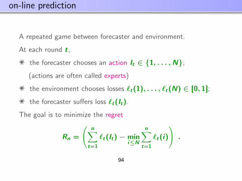
on-line prediction

A repeated game between forecaster and environment.

At each round t,

the forecaster chooses an action t 2 1, . . . , ;(actions are often called experts)

the environment chooses losses `t(1), . . . , `t(N) 2 [0, 1];

the forecaster su↵ers loss `t(It).

The goal is to minimize the regret

Rn =

Xn n

`t(It) min

it

N=1

X`t(i)

t=1

!.

7

I N

94

simplest example

Is it possible to make (1/n)Rn ! 0 for all loss assignments?

Let N = 2 and define, for all t = 1, . . . , n,

`t(1) =

0 if It = 2

1 if It = 1

and `t(2) = 1 `t(1).

ThenXn n n

`t(It) = n and min `i=1 2

t=1

Xt(i)

,

t=1

2

so1 1

Rnn .

2

95

randomized prediction

Key to solution: randomization.

At time t, the forecaster chooses a probability distributionpt1

= (p1,t1

, . . . , pN,t1

)

and chooses action i with probability pi ,t1

.

Simplest model: all losses `s(i), i = 1, . . . ,N , s < t, areobserved: full information.

12

96

Hannan and Blackwell

Hannan (1957) and Blackwell (1956) showed that the forecasterhas a strategy such that

1

Xn n

`t(It)n min

it

N=1

X`t(i)

t=1

!! 0

almost surely for all strategies of the environment.

13

97

basic ideas

expected loss of the forecaster:

N

`t(pt1

) =

Xpi ,t (1

`t i) = Et`t(It)i=1

By martingale convergence, Xn n

1

` ` 1 2

t(It) X

/t(pn t1

) = OP(n)

t=1 t=1

so it suces to study

1

n

Xn n

`t(pt ) min ` (i)1

N

=1

Xt

it t=1

!

!

98

weighted average prediction

Idea: assign a higher probability to better-performing actions.Vovk (1990), Littlestone and Warmuth (1989).

A popular choice is

exp

Pt1

=1

` (s s i)pi ,t =1

P = 1

N=1

exp

P i , . . . ,N .t1

=1

`s( )k s k

where > 0. Then

1

Xn

n

n

`t(pt1

) min

it=1

N

X`t(i)

t=1

!=

rlnN2n

with =

p8 lnN/n.

99

proof

tLet Li ,t =

Ps=1

`s(i) and

N

Wt =

X XNwi ,t = eLi ,t

i=1 i=1

for t 1, and W0

= N . First observe that

Wnln e

W

XN= ln

,

0

Li n

i=1

! lnN

ln

max eLi ,n

ln

i=1,...,N

N

= min Li ,ni=1,...,N

lnN .

100

proof

On the other hand, for each t = 1, . . . , n

WtPN

i=1

wi ,t 1

e`t(i)ln = ln

Wt1

PN

Pj=1

wj ,t1

N=1

wP

i ,t1

` (

i t i) 2 +N

8j=1

wj ,t1

2= `t(pt1

) +

8

by Hoe↵ding’s inequality.

Hoe↵ding (1963): if X 2 [0, 1],

lnEe 2X EX +

8101

proof

for each t = 1, . . . , n

W 2

t ln `t(p ) +

W tt1

1

8

Summing over t = 1, . . . , n,

W nn

ln X 2

`t(pt 1

) + n .W

0

8

t=1

Combining these, we get

XnlnN

`t(pt 1

) min Li ,n + + n i=1,...,N 8

t=1

102

lower bound

The upper bound is optimal: for all predictors,Pn

=1

`t(Itp n

) mint iN `tsup

=1

t(i)1 .

n,N,`t(i) (n/2) lnN

P

Idea: choose `t(i) to be i.i.d. symmetric Bernoulli coin flips.

n

sup

Xn

`t(It)t(i)

min

` it=1

N

X`t(i)

" t=1

!

n

EX

`t(It) min

it=1

N

n

Xn

`t(i)t=1

#

=

2

minBiiN

Where B1

, . . . ,BN are independent Binomial (n, 1/2).Use the central limit theorem. 103

follow the perturbed leader

t1

It = argminX

`s(i) + Zi ,ti=1,...,N s=1

where the Zi ,t are random noise variables.

The original forecaster of Hannan (1957) is based on this idea.

104

follow the perturbed leader

If the Zi ,t are i.i.d. uniform [0,p

nN], then

1 NRnn

2

r+ Op(n1/2

) .n

If the Z zi ,t are i.i.d. with density (/2)e| |, then for

plogN/n,

1 logNR 1/2

n cr

+ Op(n) .

n n

Kalai and Vempala (2003).

105

combinatorial experts

Often the class of experts is very large but has some combinatorialstructure. Can the structure be exploited?

path planning. At each timeinstance, the forecaster chooses apath in a graph between twofixed nodes. Each edge has anassociated loss. Loss of a path isthe sum of the losses over theedges in the path.

N is huge!!!

© Google. All rights reserved. This content is excluded from ourCreative Commons license. For more information, seehttp://ocw.mit.edu/fairuse.

106

http://ocw.mit.edu/fairuse

assignments: learning permutations

Given a completebipartite graphKm,m, theforecaster chooses aperfect matching.The loss is the sumof the losses overthe edges.

Helmbold and Warmuth (2007): full information case.

This image has been removed due to copyright restrictions.Please see the image athttp://38.media.tumblr.com/tumblr_m0ol5tggjZ1qir7tc.gif

107

http://38.media.tumblr.com/tumblr_m0ol5tggjZ1qir7tc.gif

spanning trees

The forecaster chooses aspanning tree in the completegraph Km. The cost is the sumof the losses over the edges.

108

combinatorial experts

dFormally, the class of experts is a set S 0, 1 of cardinality|S| = N .

t 2 RdAt each time , a loss is assigned to each component: `t .

Loss of expert v 2 S is `t(v) = `>t v .

Forecaster chooses It 2 S.

The goal is to control the regret

Xn Xn

`t(It) min `t(k) .k=1,...,N

t=1 t=1

109

computing the exponentially weighted average forecaster

One needs to draw a random element of S with distributionproportional to

wt(v) = exp

t

Lt(v)= exp

1

X

`>t v .s=1

!

t

exp

j

Yd=

=1

1

X

`t,jvjs=1

!.

110

computing the exponentially weighted average forecaster

path planning: Sampling may be done by dynamic programming.

assignments: Sum of weights (partition function) is the permanentof a non-negative matrix. Sampling may be done by a FPAS ofJerrum, Sinclair, and Vigoda (2004).

spanning trees: Propp and Wilson (1998) define an exact samplingalgorithm. Expected running time is the average hitting time ofthe Markov chain defined by the edge weights wt(v).

111

computing the follow-the-perturbed leader forecaster

In general, much easier. One only needs to solve a linearoptimization problem over S. This may be hard but it is wellunderstood.

In our examples it becomes either a shortest path problem, or anassignment problem, or a minimum spanning tree problem.

112

follow the leader: random walk perturbation

Suppose N experts, no structure. Define

t

It = argmin (`i ,s 1

+ Xs)i=1,...,N

X

s=1

where the Xs are either i.i.d. normal or ±1 coinflips.

This is like follow-the-perturbed-leader but with random walktperturbation: s=1

Xt .

Advantage: fo

P

recaster rarely changes actions!

113


If Rn is the regret and Cn is the number of times It 6= It1

, then

ERn 2ECn 8

p2n logN + 16 log n + 16 .

Devroye, Lugosi, and Neu (2015).

Key tool: number of leader changes in N independent randomwalks with drift.

114


This also works in the “combinatorial” setting: just add anindependent N(0, d) at each time to every component.

ERn = Oe(B3/2p

n log d)

andECn = O(B

pn log d) ,

where B = maxv2S kvk1

.

115

why exponentially weighted averages?

May be adapted to many di↵erent variants of the problem,including bandits, tracking, etc.

116

multi-armed bandits

The forecaster only observes `t(It) but not `t(i) for i 6= It .

Herbert Robbins (1952).

This image has been removed due to copyright restrictions. Please see the image athttps://en.wikipedia.org/wiki/Herbert_Robbins#/media/File:1966-HerbertRobbins.jpg

117

https://en.wikipedia.org/wiki/Herbert_Robbins#/media/File:1966-HerbertRobbins.jpg

multi-armed bandits

Trick: estimate `t(i) by

e `t(It)t(i

I =i) =

t pIt ,t1

This is an unbiased estimate:

e XN `t(j)Et`t(i) = pj ,t 1

j=i= `t(i)

jj ,=1

p t1

Use the estimated losses to define exponential weights and mixwith uniform (Auer, Cesa-Bianchi, Freund, and Schapire, 2002):

Ptexp 1 ` ( )

P s=1

pi ,t 1 es i

1

= ( ) Nk=1

exp

P +

t1

s=1

`s(k)

Nexploration

e| z

exploitation

|z

118

multi-armed bandits

Xn1

E

`t(pt 1

) min

Xn

`t(i)

!= O

rN lnN

!,

n it=1

Nt=1

n

119

multi-armed bandits

Lower bound:

n1 N

sup E Xn

`t(pt 1

) min

X`t(i) ,

`t(i) n i N=1

=1

! C

r

nt t

Dependence on N is not logarithmic anymore!

Audibert and Bubeck (2009) constructed a forecaster with

n n1 N

maxE `t(pti 1

) `t(i) = O ,N n

t=1 t=1

! r

n

!X X

120

calibration

Sequential probability assignment.

A binary sequence x1

, x2

, . . . is revealed one by one.

After observing x1

, . . . , xt1

, the forecaster issues predictionIt 2 0, 1, . . . ,N.Meaning: “chance of rain is It/N”.

Forecast is calibrated ifP n

t=1

xt

It=iPn

t=1

It=i

iN

1

2N+ o(1)

whenever lim supn(1/n)Pn

t=1

0It=i > .

Is there a forecaster that is calibrated for all possible sequences?NO. (Dawid, 1985). 121

randomized calibration

However, if the forecaster is allowed to randomize then it ispossible! (Foster and Vohra, 1997).

This can be achieved by a simple modification of any regretminimization procedure.

Set of actions (experts): 0, 1, . . . ,N.At time t, assign loss `t(i) = (xt i/N)

2 to action i .

One can now define a forecaster. Minimizing regret is notsucient.

122

internal regret

Recall that the (expected) regret is

Xn

`t(pt

Xn n

1

) min `t(i) = max i it=1 t=1

Xpj ,t (`t(j) `t(i))

t=1

X

j

The internal regret is defined by

n

max

Xpj ,t (`t(j) `t(i))

i ,jt=1

pj ,t (`t(j) `t(i)) = Et `It=j ( t(j) `t(i))

is the expected regret of having taken action j instead of action i .123

internal regret and calibration

By guaranteeing small internal regret, one obtains a calibratedforecaster.

This can be achieved by an exponentially weighted averageforecaster defined over N2 actions.

Can be extended even for calibration with checking rules.

124

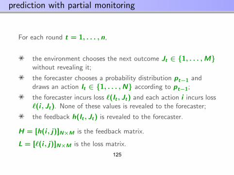
prediction with partial monitoring

For each round t = 1, . . . , n,

the environment chooses the next outcome Jt 2 1, . . . ,Mwithout revealing it;

the forecaster chooses a probability distribution pt and1

draws an action It 2 1, . . . ,N according to pt1

;

the forecaster incurs loss `(It , Jt) and each action i incurs loss`(i , Jt). None of these values is revealed to the forecaster;

the feedback h(It , Jt) is revealed to the forecaster.

H = [h(i , j)]NM is the feedback matrix.

L = [`(i , j)]NM is the loss matrix.

125

examples

Dynamic pricing. Here M = N , and L = [`(i , j)]NN where

(j )

i j i ij + c

( , ) =

i>j`

.

N

and h(i , j) = i>j or

h(i , j) = a i j + b i>j , i , j = 1, . . . ,N .

Multi-armed bandit problem. The only information the forecasterreceives is his own loss: H = L.

126

examples

Apple tasting. = = 2.

L =

0 1

1 0

H =

a ab c

.

The predictor only receives feedback when he chooses the secondaction.Label ecient prediction. N = 3, M = 2.

L =

21 1

40 1

1 0

3

5

H =

2a bc c

3

.

N M

4c c

5

127

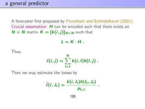
a general predictor

A forecaster first proposed by Piccolboni and Schindelhauer (2001).Crucial assumption: H can be encoded such that there exists anN N matrix K = [k(i , j)]NN such that

L = K · H .

Thus,

`(i , j) =XN

k(i , l)h(l , j) .l=1

Then we may estimate the losses by

e k(i , It)h(It , Jt)(i , Jt) = pIt ,t

.

128

a general predictor

Observe

e XN k(i , k)h(k, Jt)Et`(i , Jt) = pk,t1

k=1

pk,t1

kk

XN= (i , k)h(k, Jt) = `(i , Jt) ,

=1

e(i , Jt) is an unbiased estimate of `(i , Jt).Let

eLi ,t1 pi ,t1

= (1 )e

P +

N=1

eLek,t1 Nk

where Li ,t =

Pt=1

`(i , Jt).es

e129

performance bound

With probability at least 1 ,

1

Xn1

`(It , Jt)n min

i=1,...,Nt=1

Xn

`(i , Jt)nt=1

Cn 1/3N2/3pln(N/) .

where C depends on K . (Cesa-Bianchi, Lugosi, Stoltz (2006))

Hannan consistency is achieved with rate O(n1/3) whenever

L = K · H .

This solves the dynamic pricing problem.

Bartok, Pal, and Szepesvari (2010): if M = 2, only possible ratesare n1/2, n1/3, 1

130

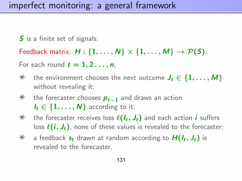
imperfect monitoring: a general framework

S is a finite set of signals.

Feedback matrix: H : 1, . . . ,N 1, . . . ,M ! P(S).

For each round t = 1, 2 . . . , n,

the environment chooses the next outcome Jt 2 1, . . . ,Mwithout revealing it;

the forecaster chooses pt1

and draws an actionIt 2 1, . . . ,N according to it;

the forecaster receives loss `(It , Jt) and each action i su↵ersloss `(i , Jt), none of these values is revealed to the forecaster;

a feedback st drawn at random according to H(It , Jt) isrevealed to the forecaster.

131

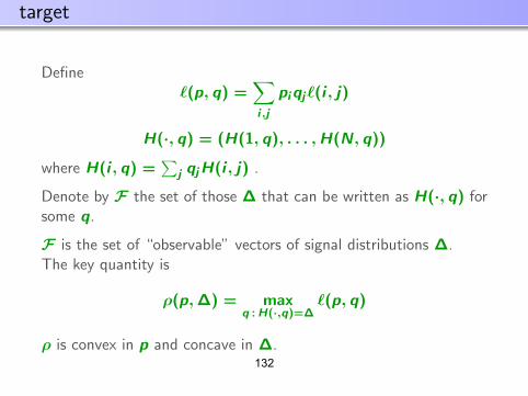
target

Define`(p, q) =

Xpiqj`(i , j)

i ,j

H(·, q) = (H(1, q), . . . ,H(N, q))

where H(i , q) = j qjH(i , j) .

Denote by F the set

P

of those that can be written as H(·, q) forsome q.

F is the set of “observable” vectors of signal distributions .The key quantity is

(p,) = max `(p, q)q :H(·,q)=

is convex in p and concave in .132

rustichini’s theorem

The value of the base one-shot game is

minmax `(p, q) = min max (p,)

p q p2F

If qn is the empirical distribution of J1

, . . . , Jn, even with theknowledge of H(·, qn) we cannot hope to do better thanminp (p,H(·, qn)).

Rustichini (1999) proved that there exists a strategy such that forall strategies of the opponent, almost surely,

lim sup

0

@1

X`(It , Jt) min (p,H(

n n!1 p·, qn))

t=1,...,n

1

A 0

133

rustichini’s theorem

Rustichini’s proof relies on an approachability theorem for acontinuum of types (Mertens, Sorin, and Zamir, 1994).

It is non-constructive.

It does not imply any convergence rate.

Lugosi, Mannor, and Stoltz (2008) construct eciently computablestrategies that guarantee fast rates of convergence.

134

combinatorial bandits

The class of actions is a set S 0 d, 1 of cardinality |S| = N .

At each time t d, a loss is assigned to each component: `t 2 R .

Loss of expert v 2 S is `t(v) = `>t v .

Forecaster chooses It 2 S.

The goal is to control the regret

Xn n

`t(It) min

k=1,...,Nt=1

X`t(k) .

t=1

135

combinatorial bandits

Three models.

(Full information.) All d components of the loss vector areobserved.

(Semi-bandit.) Only the components corresponding to the chosenobject are observed.

(Bandit.) Only the total loss of the chosen object is observed.

Challenge: Is O(n1/2poly(d)) regret achievable for thesemi-bandit and bandit problems?

136

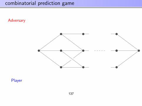
combinatorial prediction game

Adversary

Player

137


Adversary

Player

`2

`6

`d1

`1

`4

`5

`9

`d2

`d`3

`8

`7


140



Adversary

Player

`2

`6

`d1

`1

`4

`5

`9

`d2

`d`3

`8

`7

loss su↵ered: `2

+ `7

+ . . . + `d


141



Adversary

Player

`2

`6

`d1

`1

`4

`5

`9

`d2

`d`3

`8

`7

<8

Full Info: `1

, `2

, . . . , `dFeedback: :

loss su↵ered: `2

+ `7

+ . . . + `d


142



Adversary

Player

`2

`6

`d1

`1

4

`5

`9

`d2

`d`3

`8

`7

`

< n db ck:

8Full I fo: `

1

, `2

, . . . , `Feed a : Semi-Bandit: `

2

, `7

, . . . , `dBandit: `

2

+ `7

+ . . . + `d

loss su↵ered: `2

+ `7

+ . . . + `d


143


notation

`2

`6

`d1

`1

`4

`5

`9

`d2

`d`3

`8

`7

`2

`6

`d1

`1

`4

`5

`9

`d2

`d`3

`8

`7

S 0, 1d

`t 2 Rd+

Vt 2 S T, loss su↵ered: `t Vt

regret:n

R EX n

TV EX

Tn = `t t min `t u

ut=1

2St=1

Tloss assumption: `t v 1 for all v and t = 1, . . . , n.| | 2 S144

weighted average forecaster

At time t assign a weight wt,i to each i = 1, . . . , d .

The weight of each vk 2 S is

w t(k) = wt,i .i :vk

Y

(i)=1

Let qt1

(k) = w t1

(k N)/ k=1

w t1

(k).

At each time t, draw Kt from

P

the distribution

pt1

(k) = (1 )qt k1

( ) + µ(k)

where µ is a fixed distribution on S and > 0. Here

wt,i = exp Lt,i

where Lt,i = `1,i + + `t,i and

`t,i is a

n estimated loss.

e

e e · · · e e145

loss estimates

Dani, Hayes, and Kakade (2008).Define the scaled incidence vector

X t = `t(Kt)V Kt

where Kt is distributed according to pt1

.

Let Pt1

= EV Kt V> be theKt

d d correlation matrix.Hence

Pt 1

(i , j) =k : vk(i

Xpt1

(k) .)=vk(j)=1

Similarly, let Qt1

and M be the correlation matrices of E V V>

when V has law, qt1

and µ. Then

Pt1

(i , j) = (1 )Qt1

(i , j) + M(i , j) .

The vector of loss estimates is defined by

et = P+

t1

X t

where P+

t1

is the pseudo-inverse of Pt1

.146

key properties

M M+v = v for all v 2 S.

Qt1

is positive semidefinite for every t.Pt 1

P+ r at 1

v = v fo ll t v and 2 S.

By definition,Et X t = Pt1

`t

and thereforeEt et = P+

t1

Et X t = `t

An unbiased estimate!

147

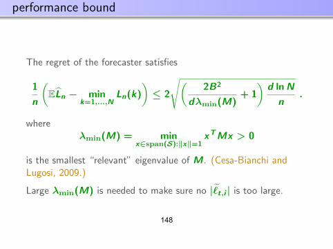
performance bound

The regret of the forecaster satisfies

1

ln

ELb2B2 d N

n min Ln(k) 2 + 1 .n k=1,...,N

s

dmin(M)

n

whereTmin(M) = min x Mx > 0

x2span(S):kxk=1

is the smallest “relevant” eigenvalue of M . (Cesa-Bianchi andLugosi, 2009.)

Large min(M) is needed to make sure no `t,i is too large.|e |

148

performance bound

Other bounds:

Bp

d lnN/n (Dani, Hayes, and Kakade). No condition on S.Sampling is over a barycentric spanner.

dp

( ln n)/n (Abernethy, Hazan, and Rakhlin). Computationallyecient.

149

eigenvalue bounds

min(M) = min E(V , x)2 .x2span(S):kxk=1

where V has distribution µ over S.

In many cases it suces to take µ uniform.

150

multitask bandit problem

The decision maker acts in m games in parallel.In each game, the decision maker selects one of R possible actions.After selecting the m actions, the sum of the losses is observed.

1

min =

R

maxE Ln Ln(k) lnR .k

2mp3nR

The price of only obs

hb

erving the su

i

m of losses is a factor of m.

Generating a random joint action can be done in polynomial time.

151

assignments

Perfect matchings of Km,m.At each time one of the N = m! perfect matchings of Km,m isselected.

1

min(M) =

m 1

maxE Ln Ln(k) 2m 3n ln(m!) .k

Only a factor of m

h

w

b

orse than n

i

aive full-i

p

nformation bound.

152

spanning trees

In a network of m nodes, the cost of communication between twonodes joined by edge e is `t(e) at time t. At each time a minimalconnected subnetwork (a spanning tree) is selected. The goal is tominimize the total cost. N = mm2.

1

min(M) =

1

Om

m2

.

The entries of M are

2

PVi = 1=m

P

3

Vi = 1, Vj = 1

= if

m2

i j

4

P Vi = 1, Vj = 1 = if .2

i 6 jm

153

stars

At each time a central node of a network of m nodes is selected.Cost is the total cost of the edges adjacent to the node.

1

min 1 O

m

.

154

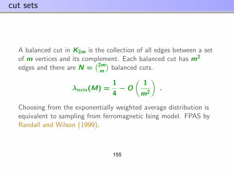
cut sets

A balanced cut in K2m is the collection of all edges between a set

of m vertices and its complement. Each balanced cut has m2

2medges and there are N = m

balanced cuts.

1 1

min(M) = O .4

m2

Choosing from the exponentially weighted average distribution isequivalent to sampling from ferromagnetic Ising model. FPAS byRandall and Wilson (1999).

155

hamiltonian cycles

A Hamiltonian cycle in Km is a cycle that visits each vertex exactlyonce and returns to the starting vertex. N = (m 1)!

2

min m

Ecient computation is hopeless.

156

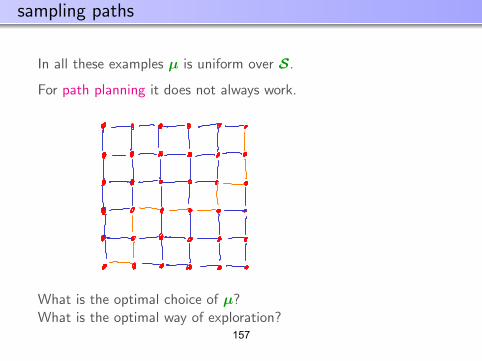
sampling paths

In all these examples µ is uniform over S.

For path planning it does not always work.

What is the optimal choice of µ?What is the optimal way of exploration?

157

minimax regret

Rn = inf max sup Rnstrategy S0,1d adversary

Theorem

Let n d 2. In the full information and semi-bandit games, wehave

0.008 dp

n Rn dp2n,

and in the bandit game,

0.01 d 3/2pn Rn 2 d 5/2p2n.

158

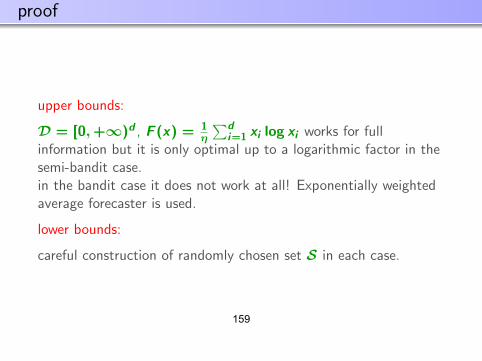
proof

upper bounds:

D = [0,+1)

d , F (x) = 1

dog i=1

xi l xi works for fullinformation but it is only opti

P

mal up to a logarithmic factor in thesemi-bandit case.in the bandit case it does not work at all! Exponentially weightedaverage forecaster is used.

lower bounds:

careful construction of randomly chosen set S in each case.

159

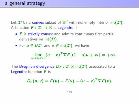
a general strategy

Let D dbe a convex subset of R with nonempty interior int(D).A function F : D ! R is Legendre if

• F is strictly convex and admits continuous first partialderivatives on int(D),

• For u 2 @D, and v 2 int(D), we have

lim (u v T) rF

(1 s)u + sv = +

s!0,s>0

1.

The Bregman divergence DF : D int(

D) associated to aLegendre function F is

DF (u T, v) = F (u) F (v) (u v) rF (v).

160

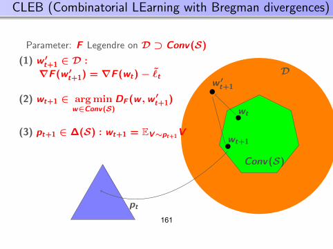
CLEB (Combinatorial LEarning with Bregman divergences)

Parameter: F Legendre on D Conv(S)

Conv(S)

D

(S)

pt

wt

w 0t+1

wt+1

pt+1

(1) wt0+1

2 D :

rF (w 0+1

) = rF ( )t wt `˜t

(2) wt+1

2 argmin DF (w ,wt0+1

)

w2Conv(S)

(3) pt+1

2 (S) : wt+1

= EVpt+1

V

161

General regret bound for CLEB

Theorem

If F admits a Hessian r2F always invertible then,

n

Rn / diam T 2

1

˜DF (S) + EX

`t=1

r F (wt)

t

`t .

162

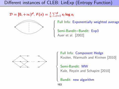
Di↵erent instances of CLEB: LinExp (Entropy Function)

D 1Pd

= [0,+ )

d , F (x) = 1

i=1

xi log xi

8>><

Full Info: Exponentially weighted average

>>: Semi-Bandit=Bandit: Exp3Auer et al. [2002]

8>>>

Full Info: Component Hedge

>>>> Koolen, Warmuth and Kivinen [2010]><

>>Semi-Bandit: MW

>> Kale, Reyzin and Schapire [2010]

Bandit: new algorithm

>>>>:

163

Di↵erent instances of CLEB: LinINF (ExchangeableHessian)

D = [0,+1)

d , F (x) =Pd

i=1

R xi 1

( )

0

s ds

INF, Audibert and Bubeck [2009]

(x) = exp(x) : LinExp (x) = (x)q, q > 1 : LinPoly

164

Di↵erent instances of CLEB: Follow the regularized leader

D = Conv(S), then

wt+1

2 argmin

Xt

T`s w + F (w)

w2D s=1

!

Particularly interesting choice: F self-concordant barrier function,Abernethy, Hazan and Rakhlin [2008]

165


Lecturer: Philippe Rigollet Lecture 1Scribe: Haihao (Sean) Lu Nov. 2, 2015

3. STOCHASTIC BANDITS

3.1 Setup

The stochastic multi-armed bandit is a classical model for decision making and is definedas follows:

There are K arms(different actions). Iteratively, a decision maker chooses an arm k ∈1, . . . ,K, yielding a sequence XK,1, . . . ,XK,t, . . ., which are i.i.d random variables withmean µk. Define µ∗ = maxj µj or ∗ ∈ argmax. A policy π is a sequence πtt≥1, whichindicates which arm to be pulled at time t. πt ∈ 1, . . . ,K and it depends only on theobservations strictly interior to t. The regret is then defined as:

n n

Rn = max IE[ XK,t]− IE[ Xπt,t]k

∑

t=1

∑

t=1n

= nµ∗ − IE[∑

Xπt,t]t=1

n

= nµ∗ − IE[IE[

K

∑

Xπt,t | πt]]t=1

=∑

∆kIE[Tk(n)] ,k=1

nwhere ∆k = µ∗ − µk and Tk(n) =∑

t=1 1I(πt = k) is the number of time when arm k waspulled.

3.2 Warm Up: Full Info Case

X1,t.Assume in this subsection that K = 2 and we observe the full information

..

at

XK,t

time t after choosing πt. So in each iteration, a normal idea is to choose

the arm

withhighest average return so far. That is

¯πt = argmaxXk,tk=1,2

where1

Xk,t =t

t∑

s=1

Assume from now on that all random variable Xk,t are subGaussian with variance proxy2 2

σ2, which means IE[euxu σ

] ≤ e 2 for all u ∈ IR. For example, N(0, σ2) is subGaussian with

Xk,s

8

166

variance proxy σ2 and any bounded random variable X ∈ [a, b] is subGaussian with varianceproxy (b− a)2/4 by Hoeffding’s Lemma.

Therefore,Rn = ∆IE[T2(n)] , (3.1)

where ∆ = µ1 − µ2. Besides,

n

¯ ¯T2(n) = 1 +∑

1I(X2,t > X1,t)t=2n

= 1 +∑

¯ ¯1I(X2,t −X1,t − (µ2 − µ1) ≥ ∆) .t=2

¯ ¯It is easy to check that (X2,t−X1,t)−(µ2−µ1) is centered subGaussian with variance proxy2σ2, whereby

2

¯ ¯ − t∆

IE[1I(X 22,t > X1,t)] ≤ e 4σ

by a simple Chernoff Bound. Therefore,

∞2

Rn ≤ ∆(1 +∑ 4σ2

− t∆

e 24σ ) ≤ ∆+ , (3.2)∆

t=0

whereby the benchmark is4σ2

Rn ≤ ∆+ .∆

3.3 Upper Confidence Bound (UCB)

Without loss of generality, from now on we assume σ = 1. A trivial idea is that after spulls on arm k, we use µk,s = 1 ∑

j∈pulls of kXK,j and choose the one with largest µk,s.sThe problem of this trivial policy is that for some arm, we might try it for only limitedtimes, which give a bad average and then we never try it again. In order to overcome thislimitation, a good idea is to choose the arm with highest upper bound estimate on the meanof each arm at some probability lever. Note that the arm with less tries would have a largedeviations from its mean. This is called Upper Confidence Bound policy.

167

Algorithm 1 Upper Confidence Bound (UCB)

for t = 1 to K doπt = t

end forfor t = K + 1 to n do

t−1

Tk(t) =∑

1I(πt = k)s=1

(number of time we have pull arm k before time t)

1µk,t =

∑

XK,t∧sTk(t) s=1

log t)πt ∈ argmax

2 (µk,t + 2

k∈[K]

√

Tk(t)

,

end for

Theorem: The UCB policy has regret

K∑ log n π2

Rn ≤ 8 + (1 + )∆k 3

k,∆k>0

∑

∆k

k=1

Proof. From now on we fix k such that ∆k > 0. Then

n

IE[Tk(n)] = 1 +t=

∑

IP(πt = k) .K+1

Note that for t > K,

2 log t 2 log tπt = k ⊆ µk,t + 2

√

≤ µ∗,t + 2 Tk(t)

√

T∗(t) √

2 log t√

⋃ 2 log t 2 log t⊆ µk ≥ µk,t + 2 µ∗ ≥ µ∗,t + 2

⋃

µ∗ ≤ µk + 2Tk(t) T∗(t)

√

, πt = kTk(t)

And from a union bound, we have

√

2 log t 2 log tIP(µk,t − µk < −2 ) = IP(µk,t − µk < 2

Tk(t)

√

)Tk(t)

t−s8 log t

≤∑

exp( s )2

s=1

1=

t3

t−1

168

2 log t 2 log tThus IP(µk > µk t + 2k

) ≤ 1, 3 and similarly we have IP(µ∗ > µ∗,t + 2 ) ≤ 1 ,T (t) t T 3

∗(t) t

whereby

√ √

n n n∑ 1 2 log tIP(πt = k) ≤ 2 µk + 2

√∑

+∑

IP(µ∗ ≤ , πt = k)t3 Tk(t)t=K+1 t=1 t=1

∞ n1 8 log t

≤ 2∑

+∑

IP(Tk(t) ≤ , πt = k)t3 ∆2

t=1 t=1 k

∞ n

≤ 2∑ 1 g n

+∑ 8 lo

IP(Tk(t) ≤ , πt = k)t3 ∆2

t=1 t=1 k

∞ ∞∑ 1 8 o≤ 2 + (

3t=1

∑ l g nIP s ≤ )

t ∆2s=1 k

∞

≤ 2∑ 1 8 log n

+t2 ∆2

t=1 k

π2 8 log n= + ,

3 ∆2k

where s is the counter of pulling arm k. Therefore we have

K

Rn =∑ ∑ π2 8 log n

∆kIE[Tk(n)] ≤ ∆k(1 + + ) ,3 ∆2

k k,∆k

k=1 >0

which furnishes the proof.

Consider the case K = 2 at first, then from the theorem above we know Rn ∼ logn ,∆which is consistent with intuition that when the difference of two arm is small, it is hard todistinguish which to choose. On the other hand, it always hold that Rn ≤ n∆. Combining

logn log(n∆2)these two results, we have Rn ≤ ∧ n∆, whereby Rn ≤ up to a constant.∆ ∆Actually it turns out to be the optimal bound. When K ≥ 3, we can similarly get the

log(n∆2)result that Rn ≤

∑k

kk

. This, however, is not the optimal bound. The optimal bound∆

should be∑ log(n/H)

kk

, which includes the harmonic sum and H = 1 . See [Lat15].∆

∑

k ∆2

k

3.4 Bounded Regret

From above we know UCB policy can give regret that increases with at most rate log n withn. In this section we would consider whether it is possible to have bounded regret. Actuallyit turns out that if there is a known separator between the expected reward of optimal armand other arms, there is a bounded regret policy.

We would only consider the case when K = 2 here. Without loss of generality, weassume µ1 =

∆ and µ ∆2 = − , then there is a natural separator 0.2 2

169

Algorithm 2 Bounded Regret Policy (BRP)

π1 = 1 and π2 = 2for t = 3 to n doif maxk µk,t > 0 then

then πt = argmaxk µk,t

elseπt = 1, πt+1 = 2

end ifend for

Theorem: BRP has regret16

Rn ≤ ∆+ .∆

Proof.

IP(πt = 2) = IP(µ2,t > 0, πt = 2) + IP(µ2,t ≤ 0, πt = 2)

Note that

n n∑

IP(µ2,t > 0, πt = 2) ≤ IE 1I(µ2,t > 0, πt = 2)t=3

∑

t=3n

≤ IE∑

1I(µ2,t − µ2 > 0, πt = 2)t=3

∞

≤∑ 2

e−s∆

8

s=1

8= ,

∆2

where s is the counter of pulling arm 2 and the third inequality is a Chernoff bound.Similarly,

n n∑

IP(µ2,t ≤ 0, πt = 2) =∑

IP(µ1,t ≤ 0, πt−1 = 1)t=3 t=3

8≤ ,

∆2

Combining these two inequality, we have

16Rn ≤ ∆(1 + ) ,

∆2

170


Lecturer: Alexander Rakhlin Lecture 19Scribe: Kevin Li Nov. 16, 2015

4. PREDICTION OF INDIVIDUAL SEQUENCES

In this lecture, we will try to predict the next bit given the previous bits in the sequence.Given completely random bits, it would be impossible to correctly predict more than halfof the bits. However, certain cases including predicting bits generated by a human canbe correct greater than half the time due to the inability of humans to produce trulyrandom bits. We will show that the existence of a prediction algorithm that can predictbetter than a given threshold exists if and only if the threshold satifies certain probabilisticinequalities. For more information on this topic, you can look at the lecture notes athttp://stat.wharton.upenn.edu/~rakhlin/courses/stat928/stat928_notes.pdf

4.1 The Problem

To state the problem formally, given a sequence y1, . . . , yn, . . . ∈ −1,+1, we want to finda prediction algorithm yt = yt(y1, . . . , yt 1) that correctly predicts yt as much as possible.−

iidIn order to get a grasp of the problem, we will consider the case where y1, . . . , yn ∼ Ber(p).It is easy to see that we can get

n1

IE

[

n

∑

==1

yt ytt

]

→ minp, 1 − p

by letting yt equal majority vote of the first t − 1 bits. Eventually, the bit that occurswith higher probability will alway

1

s have occurred more times. So the central limit theoremshows that our loss will approach min 1p, 1− p at the rate of O(√ ).

n

Knowing that the distribution of the bits are iid Bernoulli random variables made theprediction problem fairly easy. More surprisingly is the fact that we can achieve the samefor any individual sequence.

Claim: There is an algorithm such that the following holds for any sequence y1, . . . , yn, . . ..

n1

lim sup∑

yt = yt −minyn, 1 nn n

t=1

− y ≤ 0 a.s.→∞

It is clear that no deterministic strategy can achieve this bound. For any deterministicstrategy, we can just choose yt = −yt and the predictions would be wrong every time. Sowe need a non-deterministic algorithm that chooses qt = IE[yt] ∈ [−1, 1].

To prove this claim, we will look at a more general problem. Take a fixed horizon n ≥ 1,and function φ : ±1n → R. Does

1

there exist a randomized prediction strategy such thatfor any y1, . . . , yn

n1

IE[∑

yt = ytn

t=1

] ≤ φ(y1, . . . , yn) ?

1 6

6

6

171

http://stat.wharton.upenn.edu/~rakhlin/courses/stat928/stat928_notes.pdf

For certain φ such as φ ≡ 0, it is clear that no randomized strategy exists. However for1φ ≡ , the strategy of randomly predicting the next bit (qt = 0) satisfies the inequality.2

Lemma: For a stable φ, the following are equivalent

n1

a) ∃(qt)t=1,...,n∀y1, . . . , yn IE[∑

yt = yt] ≤ φ(y1, . . . , yn)n

t=1

1b) IE[φ(ǫ1, . . . , ǫn)] ≥ where ǫ1, . . . , ǫn are Rademacher random variables

2

where stable is defined as follows

Definition (Stable Function): A function φ : ±1n → is stable if

1|φ(. . . , yi, . . .)− φ(. . . ,−yi, . . . )| ≤

n

Proof. (a =1

⇒ 1b) Suppose IEφ < . Take (y1, . . . , yn) = (ǫ1, . . .

R

, ǫn). Then IE[ 1 n yn t=1 t =2ǫt] = > IE[φ] so there must exist a sequence ( nǫ1, . . . , ǫ

1n) such that IE[

∑

∑

t yt = ǫt] >2 n =1

φ(ǫ1, . . . , ǫn).

(b =⇒ a) Recu

1

rsively define V (y1, . . . , yt) such that ∀y1, . . . , yn

1

1V (y1, . . . , yt 1) = min max

(

IE[ yt = yt] + V (y1, . . . y

1

− n)qt∈[−1,1] yt∈±1 n

)

Looking at the definition, we can see that IE[ 1 nt=1 yt = yt] = V ( )n ∅ − V (y1, . . . , yn).

Now we note that V (y1, . . . , yt) = − t − IE[φ(y1,

∑

.

1

. . , yt, ǫtn +1, . . . , ǫn)] satisfies the recursive2definition since

1 tminmax IE[ yt = yt ] IE[φ(y1, . . . , yt, ǫt+1, . . . , ǫn)]qt yt n

−

1

−2n

qtyt t 1=minmax

−− IE[φ(y1, . . . , yt, ǫt+1, . . . , ǫn)]

−

qt yt 2n−

2n

q t 1 q 1=minm x−

t − ˆ ta −

tIE[φ(y1, . . . , yt 1, 1, ǫt+1, . . . , ǫn)]− , − IE[φ(y . −1,− 1, . . , yt −1, ǫt+1, . . . , ǫn)]

−

qt 2n 2n 2n−

2n

t 1=− IE[φ(y1, . . . , yt 1, ǫt, ǫt+1, . . . , ǫ− n)]

−−

2n=V (y1, . . . , yt 1)−

The first equality uses the fact that for a, b ∈ ±1, 1a = b = −ab , the second uses the2fact that yt ∈ ±1, the third minimizes the entire expression by choosing qt so that thetwo expressions in the max are equal. Here the fact that φ is stable means qt ∈ [−1, 1] andis the only place where we need φ to be stable.

Therefore we have

1

n1

IE[∑ 1

yt = yt] = V (∅)−V (y1, . . . , yn) = −IE[φ(ǫ1, . . . , ǫn)]+ +φ(y1, . . . , yn)n 2

t=1

≤ φ(y1, . . . , yn)

1 6

66

6

6

6

6

1 6

172

by b).

By choosing φ = miny, 1− y+ c√ , this shows there is an algorithm that satisfies ourn

original claim.

4.2 Extensions

4.2.1 Supervised Learning

We can extend the problem to a regression type problem by observing xt and trying topredict yt. In this case, the objective we are trying to minimize would be

1 1l

n

∑

(yt, yt)− inff∈F

,n

∑

l(f(xt) yt)

It turns out that the best achievable performance in such problems is governed by martin-gale (or, sequential) analogues of Rademacher averages, covering numbers, combinatorialdimensions, and so on. Much of Statistical Learning techniques extend to this setting ofonline learning. In addition, the minimax/relaxation framework gives a systematic way ofdeveloping new prediction algorithms (in a way similar to the bit prediction problem).

4.2.2 Equivalence to Tail Bounds

We can also obtain probabilistic tail bound on functions φ on hypercube by using part a) ofthe earlier lemma. Rearranging part a) of the lemma we get 1− 2φ( 1y1, . . . , yn) ≤ qtyt.nThis implies

∑

2

IP( 1 µ 1 µ

φ(ǫ1, . . . , ǫn) <− )

= IP(1− 2φ(ǫ1, . . . , ǫn) > µ ≤ IP

2 n

∑

qtǫt > µ ≤ e− 2n

So IEφ ≥ 1 =⇒ existence of a strategy =⇒ tail boun

)

d for φ

(

1< .

)

2 2

We can extend the results to higher dimensions. Consider z1, . . . , zn ∈ B2 where B2 isa ball in a Hilbert space. We can define recursively y0 = 0 and yt+1 = ProjB2

(yt −1√ zt).n

Based on the properties of projections, for every ∗ ∈ , we have 1 ∑〈ˆ − ∗ 〉 ≤ 1y B2 yt y , ztn√ .n

zTaking y∗

t= ,

‖

∑

∑zt‖

n n

∀z1, . . . , zn,∑

zt√

‖t=1

‖ − n ≤∑

yt, ztt=1

〈 − 〉

Take a martingale difference sequence Z1, . . . , Zn with values in B2. Then

n n

IP(‖∑ 2

nµ

Zt

√

t=1

‖ − n > µ)≤ IP(

∑

t=1

〈yt,−Zt〉 > µ) ≤ e− 2

Integrating out the tail,

n

IE‖∑

Zt

t=1

‖ ≤ c√n

173

It can be shown using Von Neumann minimax theorem that

n n

∃(yt)∀z1, . . . , zn, y∗ ∈ B2

∑

Wt

√〈yt − y∗, zt〉 ≤ sup E c n

MDSWt 1,...,W=1 n

‖∑

t=1

‖ ≤

where the supremum is over all martingale difference sequences (MDS) with values in B2.By the previous part, this upper bound is c

√n. We conclude an interesting equivalence of

(a) deterministic statements that hold for all sequences, (b) tail bounds on the size of amartingale, and (c) in-expectation bound on this size.

In fact, this connection between probabilistic bounds and existence of prediction strate-gies for individual sequences is more general and requires further investigation.

174


Lecturer: Philippe Rigollet Lecture 20Scribe: Vira Semenova Nov. 23, 2015

In this lecture, we talk about the adversarial bandits under limited feedback. Adver-sarial bandit is a setup in which the loss function l(a, z) : AxZ is determinitic. Lim-ited feedback means that the information available to the DM after the step t is It =l(a1, z1), ..., l(at−1, zt), namely consits of the realised losses of the past steps only.

5. ADVERSARIAL BANDITS

Consider the problem of prediction with expert advice. Let the set of adversary moves be Zand the set of actions of a decision maker A = e1, ..., eK. At time t, at ∈ A and zt ∈ Z aresimultaneously revealed.Denote the loss associated to the decision at ∈ A and his adversaryplaying zt by l(at, zt). We compare the total loss after n steps to the minimum expert loss,namely:

n

min≤ ≤

∑

lt(ej , zt),1 j K

t=1

where ej is the choice of expert j ∈ 1, 2, ..,K.The cumulative regret is then defined as

n n

Rn =∑

lt(at, zt)− min∑

lt(ej , zt)1≤j≤K

t=1 t=1

The feedback at step t can be either full or limited. The full feedback setup means thatthe vector f = (l(e1, z

⊤t), ..., l(eK , zt)) of losses incurred at a pair of adversary’s choice zt and

each bandit ej ∈ e1, ..., eK is observed after each step t. Hence, the information availableto the DM after the step t is I = ∪t ′

t ′ l(a1, zt), ..., l(aK , zt =1 t′). The limited feedback meansthat the time −t feedback consists of the realised loss l(at, zt) only. Namely, the informationavailable to the DM is It = l(a1, z1), ..., l(at, zt). An example of the first setup is portfoliooptimization problems, where the loss of all possible portfolios is observed at time t. Anexample of the second setup is a path planning problem and dynamic pricing, where theloss of the chosen decision only is observed. This lecture has limited feedback setup.

The two strategies, defined in the past lectures, were exponential weights, which yieldthe regret of order Rn ≤ c

√n logK and Follow the Perturbed Leader. We would like to

play exponential weights, defined as:

1exp( tηpt,j

∑ − l= s=1 (ej , zs))

∑k

−

l=1 exp(−η∑t−1 ls=1 (ej , zs))

This decision rule is not feasible, since the loss l(ej , zt) are not part of the feedback ifej = at. We will estimate it by

l(ej , zt)1I(aˆ t = ej)l(ej , zt) =

P (at = ej)

6

175

ˆLemma: l(ej , zt) is an unbiased estimator of l(ej , zt)

K I(P ˆ l(e e =roof. E k

,zt)1 ket)

at l(ej , zt) =∑

Pk=1 (a = e ) = l(e , z )P (at=ej) t k j t

Definition (Exp 3 Algorithm): Let η > 0 be fixed. Define the exponential weightsas

−∑t−1η ˆ

(j) exp( l(ej , zs))p s=1t+1,j = ∑k

l=1 exp(−η∑t−1 ls=1 (ej , zs))

(Exp3 stands for Exponential weights for Exploration and Exploitation.)We will show that the regret of Exp3 is bounded by

√2nK logK. This bound is

√K

times bigger than the bound on the regret under the full feedback. The√K multiplier is

the price of have smaller information set at the time t. The are methods that allow to getrid of logK term in this expression. On the other hand, it can be shown that

√2nK is the

optimal regret.

−∑t

∑K

−1 ˆ W eProof. Let Wt,j = exp( kη l(e ,= j zs)), W1 t =

∑Ws j=1 t,j , and p = j=1 t,j j

t W .t

W∑K (−η

∑ −1exp t l e , z ηl e , zt+1 j=1 s=1 ( j s)) exp( ( j t))log( ) = log( ) (5.1)

W∑K e t

−

xp(−∑ −1

t η ls=1 (ej , zj=1 s))

t−1

ˆ= log(IEJ∼pt exp(−η∑

l(eJ , zs))) (5.2)s=1

≤∗ η2log(1− 2η ˆIEJ∼ptl(eJ , z

ˆs) + IEJ∼ptl (eJ , zs) (5.3)

2

∗ ˆwhere inequality is obtained by plugging in IEJ∼pt l(eJ , zt) into the inequality

η2x2expx ≥ 1− ηx+

2

.

K Kl(ej , zt)1I(a e )ˆIEJ∼pt l(eJ zt) =

∑ˆ t = j

, pt,j l(eJ , zt) =∑

pt,j = l(at, zt) (5.4)P (at = ej)j=1 j=1

K Kl22 (ej , zt)1I(a )ˆ ˆ t = ej

IEJ∼ptl (eJ , zt) =∑

pt,j l2(eJ , zt) =∑

pt,j (5.5)P 2(at = ej)j=1 j=1

l2(ej , zt) 1=

Pat,t≤ (5.6)

Pat,t

Summing from 1 through n, we get

log(Wt+1) ≤2

log( n1)− η

∑lt=1 (at, zt) +

ηW 2

∑1 .

Pa ,tt

176

For t = 1, we initialize w1,j = 1, so W1 = K.

Since IE 1 pJ =Pa ,t

∑K j,t Kj=1 = , the expression above becomespt j,t

IE log( n η2KnWn+1)− logK ≤ −η∑

t l a=1 ( t, zt) + 2ˆNoting that log(Wn+1) = log(

∑Kj=1 exp(−η

∑t−1 l e , zs=1 ( j s))and defining j∗ = argmin1≤j≤K

∑n lt=1 (ej , zt), we obtain:

K t−1 t−1

log(Wn+1) ≥ log(∑

exp(−η∑

l(ej , zs))) = −η∑

l(ej , zs)j=1 s=1 s=1

Together:

n nlogK ηKn∑

l(at, zt)− min t≤j≤

∑

l(ej , z )K

t t=1

≤ +1 η 2

=1

The choice of η :=√2 logKnK yields the bound Rn

√≤ 2K logKn.

177


Lecturer: Philippe Rigollet Lecture 21Scribe: Ali Makhdoumi Nov. 25, 2015

6. LINEAR BANDITS

Recall form last lectures that in prediction with expert advise, at each time t, the playerplays at ∈ e1, . . . , ek and the adversary plays zt such that l(at, zt) ≤ 1 for some lossfunction. One example of such loss function is linear function l(at, zt) = aTt zt where |zt|∞ ≤1. Linear bandits are a more general setting where the player selects an action at ∈ A ⊂ R

k,where A is a convex set and the adversary selects z T

t ∈ Z such that |zt at| ≤ 1. Similar tothe prediction with expert advise, the regret is defined as

Rn = E

[n n∑

TAt zt

]

−min Ta zt,a∈K

t=1

∑

t=1

where At is a random variable in A. Note that in the prediction with expert advise, the setA was essentially a polyhedron and we had min n T

a∈K aT zt=1 t = min1≤j≤k e zj t. However, in

the linear bandit setting the minimizer of aT zt can be any point of the set A and essentiallythe umber experts that the player tries to ”comp

∑

ete” with are infinity. Similar, to theprediction with expert advise we have two settings:

1 Full feedback: after time t, the player observes zt.

2 Bandit feedback: after time t, the player observes ATt zt, where At is the action that

player has chosen at time t.

We next, see if we can use the bounds we have developed in the prediction with expertadvise in this setting. In particular, we have shown the following bounds for predictionwith expert advise:

1 Prediction with k expert advise, full feedback: Rn√

≤ 2n log k.

2 Prediction with k expert advise, bandit feedback: Rn√

≤ 2nk log k.

The idea to deal with linear bandits is to discretize the set A. Suppose that A is bounded(e.g., A ⊂ B2, where B2 is the l2 ball in R

k). We can use a 1 -covering ofn A which wehave shown to be of size (smaller than)O(nk). This means there exist y1, . . . , y|N | such that

for any a ∈ A, there exist yi such that ||yi − a|| ≤ 1 . We now can bound the regret forngeneral case, where the experts can be any point in A, based on the regret on the discreteset, N = y1, . . . , y|N |,as follows.

Rn = E

[n

]n∑

TAt ztt 1

−min Ta zta∈A

= t=1[

n

∑

n

= E

∑TAt zt

]

−min Ta zt + o(1).a∈N

t=1

∑

t=1

Therefore, we restrict actions At to a combination of the actions that belong to y1, . . . , y|N |(we can always do this), then using the bounds for the prediction with expert advise, weobtain the following bounds:

178

1 Linear bandit, full feedback: Rn ≤√

2n log(nk) = O(√kn log n), which in terms

of dependency to n is of order O(√n) that is what we expect to have.

2 Linear bandit, bandit feedback: Rn ≤√

2nnk log(nk) = Ω(n), which is useless interms of dependency of n as we expect to obtain O(

√n) behavior.

The topic of this lecture is to provide bounds for the linear bandit in the bandit feedback.Problem Setup: Let us recap the problem formulation:

• at time t, player chooses action at ∈ A ⊂ [−1, 1]k.

• at time t, adversary chooses zt ∈ Z ⊂ Rk, where aTt zt = 〈at, zt〉 ∈ [0, 1].

• Bandit feedback: player observes 〈at, zt〉( rather than zt in the full feedback setup).

Literature: O(n3/4) regret bound has been shown in [BB04]. Later on this bound hasbeen improved to O(n2/3) in [BK04] and [VH06] with ”Geometric Hedge algorithm”, whichwe will describe and analyze below. We need the following assumption to show the results:Assumption: There exist δ such that δe1, . . . , δek ∈ A. This assumption guarantees thatA has full-dimension around zero.We also discretize A with a 1 -net of size Cnk and only consider the resulting discrete setnand denote it by A, where |A| ≤ (3n)k. All we need to do is to bound

Rn = E

[n∑

TAt zt

]n

−min∑

Ta zt.a∈A

t=1 t=1

For any t and a, we define

t−1exp ηt(

(

− zs=1 ˆTs a

p a) = ,t−1

a∈A exp

∑)

(

−η zs=1 ˆTs a)

where η is a parameter (that we will

∑

choose later) an

∑

d zt is defined to incorporate the idea ofexploration versus exploitation. The algorithm which is termed Geometric Hedge Algorithm

is as follows:At time t we have

• Exploitation: with probability 1− γ draw at according to pt and let zt = 0.

• Exploration: with probability γ let at = δej for some 1k ≤ j ≤ k and zt =k j)2 〈

(a kt, zt aγ

〉 t = z eδ γ t j .

Note that δ is the the parameter that we have by assumption on the set A, and η and γare the parameters of the algorithm that we shall choose later.

Theorem: Using Geometric Hedge algorithm for linear bandit with bandit feedback,

with γ = 1 = g1/3

and η√

lo n4/3

, we haven kn

E[Rn] ≤2/3Cn√

log 3/2n k .

179

Proof. Let the overall distribution of at be qt defined as qt = (1− γ)pt + γU , where U is auniform distribution over the set δe1, . . . , δek. Under this distribution, zt is an unbiasedestimator of zt, i.e.,

kγ k (

Eat∼qt [zt] = 0(1 −j)

γ) +∑

zt ej = zt.k γ

j=1

following the same lines of the proof that we had for analyzing exponential weight algorithm,we will define

1

wt = e p za∈A

(t−

x − Tη a s

s=1

)∑ ∑

.

We then have

log

(wt+1

)

= log

(∑

Tpt(a) exp ηa ztwt

a∈

(−

A

)

)

e−2

x≤1−x+x

≤2

log

(∑

T 1( )

(

1− ˆ + 2( T 2pt a ηa zt η a zs)2

a∈A

))

( − T 1= log

(

1 +∑

)

(

ˆ + 2( T 2pt a ηa zt η a zt)2

a∈A

))

log(1+x)≤x

≤∑

T 1 2pt(T 2a)

(

−ηa zt + η (a zt)2

a∈A

)

.

Taking expectation from both sides leads to

Eat∼qt

[wt+1

log

(

wt

)]

≤ −ηEat∼qt

[

pt(a)Ta zt

a∈A

] [∑ η2

+ TEat∼qt

∑2pt(a)(a zt)

2a∈A

]

= −[ 2

T ηηE

t∼pt at zt]+ 2

Ea a ∼q pt(a)(Ta zt)

2 t t

[

a

∑

∈A

]

2qt=(1−γ)pt+γU η

=− γ

Eat∼qt

[T η

at zT 2

Et a− γ

]+ η

1 −∼U

1 t zT

a t + Eγ t a

2 t∼qt

[

pt(a)(a zt)a∈A

]

aT zt≤1 −η [ ] ηγ η2

[ ] ∑

t

≤ TEat∼qt at zt + + ∼qt

[∑

T 2Eat pt(a)(a z

1− γ 1−t)

γ 2a∈A

]

.

We next, take summation of the previous relation for t = 1 up to n and use a telescopiccancellation to obtain

n nη T ηγ η2 T 2

E [logw E+ ] ≤ [logw1]− En 1

[∑

at zt

]

+ n+ E pt(a)(a z1−

t)γ 1 γ 2

t=1−

[∑

t=1 a

∑

∈A

]

n nηγ η2

≤ E [log ]− ηE

[∑

T Tat z2w1 t

]

+ n+ E pt(a)(a zt) . (6.1)1 γ 2

t=1−

[∑

t=1 a∈A

]∑

180

Note that for all a∗ ∈ A we have

n

log(wn+1) = log

( (n

a

))∑

exp −η∈A

∑Ta zs

s=1

≥ −η∑

.s=

〈 ∗a , zs1

〉

Using E[zs] = zs, leads to

n

E [log(wn+1)] ≥ −η∑

∗a , zs . (6.2)s=1

〈〉

We also have that

log(w1) = log |A| ≤ 2k log n. (6.3)

Plugging (6.2) and (6.3) into (6.1), leads to

γ ηE[Rn] ≤ n+ E

[n

]∑∑

pt a)(T 2 n

( a t)2 k log

z + . (6.4)1− γ 2 η

t=1 a∈A

nIt remains to control the quadratic term E[∑

p a aT z 2t=1 a∈A t( )( t) . We use the fact that

|(j)

zt |, |(j)

at | ≤ 1 to obtain

∑ ]

E

[n n∑∑

T 2 T 2pt(a)(a zt) = p a)Et( qt [(a zt) ]t=1 a∈A

]∑

t=1 a

∑

∈A

n k

=∑∑ 2γ k (j)

pt(a)

(

(1− γ)0 +∑

)

[ j 2a zt ]k γ

t=1 a∈A j=1

(j) n|ajzt

|≤1

≤∑∑ k2

(a)

(2

t

)k

p = n .γ γ

t=1 a∈A

Plugging this bound into (6.4), we have

η k2 2k log nE[Rn] ≤ γn+ n + .

2 γ η

Letting lognγ = 1/3

and η =n1

√

kn4/3leads to

E[ 3/2 2/3Rn] ≤ Ck n√

log n.

Literature: The bound we just proved has been improved in [VKH07] where they showO(d3/2

√n log n) bound with a better exploration in the algorithm. The exploration that we

used in the algorithm was coordinate-wise. The key is that we have a linear problem and wecan use better tools from linear regression such as least square estimation. However, we willdescribe a slightly different approach in which we never explore and the exploration is com-pletely done with the exponential weighting. This approach also gives a better performancein terms of the dependency on k. In particular, we obtain the bound O(d

√n log n) which

coincides with the bound recently shown in [BCK 12] using a John’s ellipsoid.

181

−1Theorem: Let Ct = Eat∼qt[a aTt ], zt = (aTt t zt)Ct at, and γ = 0 (so that pt = qt). Using

Geometric Hedge algorithm with η = 2√

logn for linear bandit with bandit feedbackn

leads to

E[Rn] ≤ CK√

n log n.

Proof. We follow the same lines of the proof as the previous theorem to obtain (6.4). Notethat the only fact that we used in order to obtain (6.4) is unbiasedness, i.e., E[zt] = zt,which holds here as well since

E[z −Et] = [ 1 TCt atat zt] =

−1C Et [ Tatat ]zt = zt.

Note that we can use pseudo-inverse instead of inverse so that invertibility is not an issue.Therefore, rewriting (6.4) with γ = 0, we obtain

[n

η ∑∑T 2 2k log n

E[Rn] ≤ Eat∼pt pt(a)(a zt)∈

]

+ .2 η

t=1 a A

We now bound the quadratic term as follows

n nT 2 T 2

Eat∼pt

[∑∑

pt(a)(a zt)

]

=∑∑

p a)Et( at∼pt (a zt)t=1 a∈A t=1 a∈A

[ ]

CT

t=C −1

n nT

t, zt=(atzt)C

tat

=∑

a) Tp a Et( z T 2tˆ a = pt(

Tt a) Tz a E ( −1 T −1at zt) Ct atat Ct a

t=1 a

∑

∈A

[ ] ∑

t=1 a

T

∑

∈A

n n|a

[

tzt|≤1 E

]

∑∑T −1 T −1 [a

≤taT

p (a)t]=Ct T −1a C Et t atat Ct a = pt(a)a Ct a

t=1 a∈A

[ ] ∑

t=1 a

∑

∈A

n n∑∑ tr(AB)=tr(BA)= ( )tr( T −1 1p t r( −

t a a C a) =∑∑

pt(a)tTCt aa )

t=1 a∈A t=1 a∈A

n n n

=∑

tr( −1C Et a∼pt[Taa ]) =

∑

tr( −1Ct Ct) = tr(Ik) = kn.t=1 t=1

∑

t=1

Plugging this bound into previous bound yields

η 2k log nE[Rn] ≤ nk + .

2 η

lognLetting η = 2√

, leads to E[Rn]n ≤ Ck√n log n.

182


Lecturer: Philippe Rigollet Lecture 22Scribe: Aden Forrow Nov. 30, 2015

7. BLACKWELL’S APPROACHABILITY

7.1 Vector Losses

David Blackwell introduced approachability in 1956 as a generalization of zero sum gametheory to vector payoffs. Born in 1919, Blackwell was the first black tenured professor atUC Berkeley and the seventh black PhD in math in the US.

Recall our setup for online linear optimization. At time t, we choose an action at ∈ ∆K

and the adversary chooses zt ∈ B∞(1). We then get a loss ℓ(at, zt) = 〈at, zt〉. In the fullinformation case, where we observe zt and not just ℓ(at, zt), this is the same as predictionwith expert advice. Exponential weights leads to a regret bound

Rn ≤

√n

2log(K).

The setup of a zero sum game is nearly identical:

• Player 1 plays a mixed strategy p ∈ ∆n.

• Player 2 plays q ∈ ∆m.

• Player 1’s payoff is p⊤Mq.

Here M is the game’s payoff matrix.

Theorem: Von Neumann Minimax Theorem

max min ⊤p Mq = min max ⊤p Mq.p∈∆n q∈∆m q∈∆m p∈∆n

The minimax is called the value of the game. Each player can prevent the other from doingany better than this. The minimax theorem implies that if there is a good response pq toany individual q, then there is a silver bullet strategy p that works for any q.

Corollary: If ∀q ∈ ∆n, ∃p such that p⊤Mq ≥ c, then ∃p such that ∀q, p⊤Mq ≥ c.

Von Neumann’s minimax theorem can be extended to more general sets. The followingtheorem is due to Sion (1958).

Theorem: Sion’s Minimax Theorem Let A and Z be convex, compact spaces, andf : A × Z → R. If f(a, ·) is upper semicontinuous and quasiconcave on Z ∀a ∈ A and

183

f(·, z) is lower semicontinuous and quasiconvex on A ∀z ∈ Z, then

inf sup f(a, z) = sup inf f(a, z).a∈A z∈Z z∈ aZ ∈A

(Note - this wasn’t given explicitly in lecture, but we do use it later.) Quasiconvex andquasiconcave are weaker conditions than convex and concave respectively.

Blackwell looked at the case with vector losses. We have the following setup:

• Player 1 plays a ∈ A

• Player 2 plays z ∈ Z

• Player 1’s payoff is ℓ(a, z) ∈ dR

We suppose A and Z are both compact and convex, that ℓ(a, z) is bilinear, and that‖ℓ(a, z)‖ ≤ R ∀a ∈ A, z ∈ Z. All norms in this section are Euclidean norms. Can wetranslate the minimax theorem directly to this new setting? That is, if we fix a set S ⊂ d

R ,and if ∀z ∃a such that ℓ(a, z) ∈ S, does there exist an a such that ∀z ℓ(a, z) ∈ S?

No. We’ll construct a counterexample. Let A = Z = [0, 1], ℓ(a, z) = (a, z), andS = (a, z) ∈ [0, 1]2 : a = z. Clearly, for any z ∈ Z there is an a ∈ A such that a = z andℓ(a, z) ∈ S, but there is no a ∈ A such that ∀z, a = z.

Instead of looking for a single best strategy, we’ll play a repeated game. At time t,player 1 plays at = at(a1, z1, . . . , at−1, zt−1) and player 2 plays zt = zt(a1, z1, . . . , at−1, zt−1).Player 1’s average loss after n iterations is

1ℓn =

n∑

ℓ(at, zt)n

t=1

Let d(x, S) be the distance between a point x ∈ dR and the set S, i.e.

d(x, S) = infs∈S

‖x− s‖.

If S is convex, the infimum is a minimum attained only at the projection of x in S.

Definition: A set S is approachable if there exists a strategy at = at(a1, z1, . . . , at−1, zt−1)¯such that limn→∞ d(ℓn, S) = 0.

Whether a set is approachable depends on the loss function ℓ(a, z). In our example, we canchoose a0 = 0 and at = zt−1 to get

n1

ℓlim n = lim∑

(zt−1, zt) = (z, z) ∈ S.n→∞ n→∞ n

t=1

So this S is approachable.

7.2 Blackwell’s Theorem

We have the same conditions on A, Z, and ℓ(a, z) as before.

184

Theorem: Blackwell’s Theorem Let S be a closed convex set of 2R with ‖x‖ ≤ R

∀x ∈ S. If ∀z, ∃a such that ℓ(a, z) ∈ S, then S is approachable.Moreover, there exists a strategy such that

2Rd ℓ( n, S) ≤ √

n

Proof. We’ll prove the rate; approachability of S follows immediately. The idea here is totransform the problem to a scalar one where Sion’s theorem applies by using half spaces.

Suppose we have a half space H = x ∈ dR : 〈w, x〉 ≤ c with S ⊂ H. By assumption,

∀z ∃a such that ℓ(a, z) ∈ H. That is, ∀z ∃a such that 〈w, ℓ(a, z)〉 ≤ c, or

maxmin〈w, ℓ(a, z)〉 ≤ c.z∈Z a∈A

By Sion’s theorem,

minmax〈w, ℓ(a, z)a∈A z∈Z

〉 ≤ c.

So ∃a∗H such that ∀z ℓ(a, z) ∈ H.This works for any H containing S. We want to choose Ht so that ℓ(at, zt) brings the

¯average ℓ ¯t closer to S than ℓt−1. An intuitive choice is to have the hyperplane W bounding

H ¯t be the separating hyperplane between S and ℓt−1 closest to S. This is Blackwell’s

¯strategy: let W be the hyperplane through πt ∈ argminµ∈S ‖ℓt−1 − µ‖ with normal vectorℓt−1 − πt. Then

H = x ∈ dR : 〈x− πt, ℓt−1 − πt〉 ≤ 0.

Find a∗H and play it.We need one more equality before proving convergence. The average loss can be ex-

panded:

t 1ℓt t−1 t

t tt

=− 1 t 1 1¯(ℓt−1 − πt) +

−πt + ℓt

t t t

Now we look at the distance of the average from S, using the above equation and thedefinition of πt+1:

d ¯(ℓ , S)2 ℓt = ‖ t − πt+1‖2

≤ ‖ℓt − πt‖2

=

∥∥∥

2t− 1 1¯(ℓt−1 − πt) + (ℓt − πt)t

∥

∥ t

ℓt

∥

=

(t− 1

)2

d ¯(ℓ 2 π 2t t 1 ¯

t−1, S) +‖ −

∥∥

‖+ 2

−〈ℓt − πt, ℓ

t t2 t2t−1 − πt〉

Since ℓt ∈ H, the last term is negative; since ℓt and πt are both bounded by R, the middle2

term is bounded by 4R2 . Letting µ2

t = t2d(ℓ 2t, S) , we have a recurrence relation

t

µ2t ≤ µ2

t−1 + 4R2,

=−

ℓ +1ℓ

185

implying

µ2n ≤ 4nR2.

Rewriting in terms of the distance gives the desired bound,

2Rd ℓ( t, S) ≤ √

n

Note that this proof fails for nonconvex S.

7.3 Regret Minimization via Approachability

Consider the case A = ∆ KK , Z = B∞(1). As we showed before, exponential weights Rn ≤

c√

n log(K). We can get the same dependence on n with an approachability-based strategy.First recall that

n n1 1Rn =

∑ 1ℓ(at, zt)−min ℓ(ej , zt)

n n j nt=1

∑

t=1

n n

= m x

[

1a

∑ 1ℓ(at, zt) ℓ(ej , zt)

j n nt=1

−∑

t=1

]

If we define a vector average loss

n1

ℓn =∑

(ℓ(at, zt)− ℓ(e1, zt), . . . , ℓ(aK

Rt, zt) et=1

− ℓ( K , zt))n

∈ ,

Rn ¯ ¯n → 0 if and only if all components of ℓn are nonpositive. That is, we need d( −ℓn, OK) → 0,where −O = x ∈ K

R : −1 ≤ xi ≤ 0, iK ∀ is the nonpositive orthant. Using Blackwell’sapproachability strategy, we get

Rn≤ d(ℓ −

n, O

√

K) ≤ c .

n K n

The K dependence is worse than exponential weights,√K instead of log(K).

How do we find a∗H? As a concrete example, let K = 2. We need a

√

∗H tp satisfy

〈 ∗w, ℓ( ∗aH , z)〉 = 〈w, 〈aH , z〉y − z〉 ≤ c

for all z. Here y is the vector of all ones. Note that c ≥ 0 since 0 is in S and therefore inH. Rearranging,

〈 ∗aH , z〉〈w, y〉 ≤ 〈w, z〉 + c,

Choosing a∗H = w will work; the inequality reduces to〈w,y〉

〈w, z〉 ≤ 〈w, z〉 + c.

Approachability in the bandit setting with only partial feedback is still an open problem.

186


Lecturer: Philippe Rigollet Lecture 23Scribe: Jonathan Weed Dec. 2, 2015

1. POTENTIAL BASED APPROACHABILITY

Last lecture, we saw Blackwell’s celebrated Approachability Theorem, which establishes aprocedure by which a player can ensure that the average (vector) payoff in a repeated gameapproaches a convex set. The central idea was to construct a hyperplane separating the

¯convex set from the point `t 1, the average loss so far. By projecting perpendicular to−this hyperplane, we obtained a scalar-valued problem to which von Neumann’s minimaxtheorem could be applied. The set S is approachable as long as we can always find a “silverbullet,” a choice of action at for which the loss vector `t lies on the side of the hyperplanecontaining S. (See Figure 1.)

Figure 1: Blackwell approachability

Concretely, Blackwell’s Theorem also implied the existence of a regret-minimizing algo-rithm for expert advice. Indeed, if we define the vector loss `t by (`t)i = `(at, zt)− `(ei, zt),then the average regret at time t is equivalent to the sup-norm distance between the average

¯loss `t and the negative orthant. Approaching the negative orthant therefore correspondsto achieving sublinear regret.

However, this reduction yielded suboptimal rates. To bound average regret, wthe sup-norm distance by the Euclidean distance, which led to an extra factor of

√e replacedk appear-

ing in our bound. In the sequel, we develop a more sophisticated version of approachabilitythat allows us to adapt to the geometry of our problem. (Much of what follows resem-bles out development of the mirror descent algorithm, though the two approaches differ incrucial details.)

1.1 Potential functions

We recall the setup of mirror descent, first described in Lecture 13. Mirror descent achievedaccelerated rates by employing a potential function which was strongly convex with respect

187

to the given norm. In this case, we seek what is in some sense the opposite: a functionwhose gradient does not change too quickly. In particular, we make the following definition.

Definition: A function Φ : IRd → IR is a potential for S ∈ IR if it satisfies the followingproperties:

• Φ is convex.

• Φ(x) ≤ 0 for x ∈ S.

• Φ(y) = 0 for y ∈ ∂S.

• Φ(y) − Φ(x) − 〈∇Φ(x), y − x〉 ≤ h x2‖ − y‖2, where by abuse of notation we use

∇Φ(x) to denote a subgradient of Φ at x.

Given such a function, we recall two associated notions from the mirror descent algo-rithm. The Bregman divergence associated to Φ is given by

DΦ(y, x) = Φ(y)− Φ(x)− 〈∇Φ(x), y − x〉 .

Likewise, the associated Bregman projection is

π(x) = argminDΦ(y, x) .y∈S

We aim to use the function Φ as a stand-in for the Euclidean distance that we employedin our proof of Blackwell’s theorem. To that end, the following lemma establishes severalproperties that will allow us to generalize the notion of a separating hyperplane.

Lemma: For any convex, closed set S and z ∈ S, x ∈ SC , the following propertieshold.

• 〈z − π(x),∇Φ(x)〉 ≤ 0,

• 〈x− π(x),∇Φ(x)〉 ≥ Φ(x).

In particular, if Φ is positive on SC , then H := y | 〈y − Φ(x),∇Φ(x)〉 = 0 is aseparating hyperplane.

Our proof requires the following proposition, whose proof appears in our analysis of themirror descent algorithm and is omitted here.

Proposition: For all z ∈ S, it holds

〈∇Φ(π(x))−∇Φ(x), π(x)− z〉 ≤ 0 .

Proof of Lemma. Denote by π the projection π(x). The first claim follows upon expandingthe expression on the left-hand side as follows

〈z − π,∇Φ(x)〉 = 〈z − π,∇Φ(x)−∇Φ(π)〉+ 〈z − π,∇Φ(π)〉.

188

The above Proposition implies that the first term is nonpositive. Since the function Φ isconvex, we obtain

0 ≥ Φ(z) ≥ Φ(π) + 〈z − π,∇Φ(π)〉 .

Since π lies on the boundary of S, by assumption Φ(π) = 0 and the claim follows.For the second claim, we again use convexity:

Φ(π) ≥ Φ(x) + 〈π − x,∇Φ(x)〉 .

Since Φ(π) = 0, the claim follows.

1.2 Potential based approachability

With the definitions in place, the algorithm for approachability is essentially the same as itbefore we introduced the potential function. As before, we will use a projection defined bythe hyperplane H = y | 〈y− ¯ ¯π(`t−1),∇Φ(`t = 0 and von Neumann’s minmax theorem−1〉 to find a “silver bullet” a∗t such that `t = `(a∗t , zt) satisfies

〈`t − ¯πt,∇Φ(`t−1)〉 ≤ 0 .

All that remains to do is to analyze this procedure’s performance. We have the followingtheorem.

Theorem: If ‖`(a, z)‖ ≤ R holds for all z ∈ A, z ∈ Z and all assumptions above aresatisfied, then

4R2h log n¯Φ(`n) ≤ .n

Proof. The definition of the potential Φ required that Φ be upper bounded by a quadraticfunction. The proof below is a simple application of that bound.

As before, we note the identity

`¯ ¯ t t−1`t = `t−1 + .

t

This expression and the definition of Φ imply.

1 h¯ ≤ ¯) 〈 ¯Φ(`t Φ(`t−1) + `t − ¯ ¯` 2t 1, )− ∇Φ(`t 1 〉+ ‖`− t `

t 2 2− t−1

t‖ .

¯The last term is the easiest to control. By assumption, `t and `t 1 are contained in a ball−of radius R, so ‖`t − ¯

t−1‖2 ≤ 4R2.To bound the second term, write

1 1 1〈 ¯`t − ¯ ¯ ¯ ¯`t 1,∇Φ(`t 1)〉 = 〈`t − πt,∇Φ(`t 1) + π ` , Φ(` ) .t

− − − 〉t〈 t

t− t−1 ∇ t−1 〉

The first term is nonpositive by assumption, since this is how the algorithm constructsthe silver bullet. By the above Lemma, the inner product in the second term is at most− ¯Φ(`t−1).

We obtain (t− 1 2¯Φ(`t) ≤

)hR2

¯Φ(`t )−1 + .t t2

− ¯

189

¯Defining ut = tΦ(`t) and rearranging, we obtain the recurrence

2hR2

ut ≤ ut−1 + ,t

Son

un =∑ n

ut − ut−1 ≤ 2hR2∑ 1

tt=1 t=1

Applying the definition of un proves the claim.

1.3 Application to regret minimization

We now show that potential based approachability provides√ an improved bound on regretminimization. Our ultimate goal is to replace the bound nk (which we proved last lecture)by√n log k (which we know to be the optimal bound for prediction with expert advice).

We will be able to achieve this goal up to logarithmic terms in n. (A more careful analysisof the potential defined below does actually yields an optimal rate.)

Recall that Rn ¯= d (`n, On K− ), where Rn is the cumulative regret after n rounds and O−∞ K

is the negative orthant. It is not hard to see that d = ‖x+‖ , where x+ is the positive∞ ∞part of the vector x.

We define the following potential function:

K1 1

Φ(x) = logη

K

∑eη(xj)+

j=1

.

The function Φ is a kind of “soft max” of the

positive entries

of x. (Note that this definition

does not agree with the use of the term soft max in the literature—the difference is thepresence of the factor 1 .) The terminology soft max is justified by noting thatK

1 1‖x+‖ = max(x log +logK logK

j)+ ≤ max eη(xj) + .η≤ Φ(x) +∞

j j η K η

The potential function therefore serves as an upper bound on the sup distance, up to anadditive logarithmic factor.

The function Φ defined in this way is clearly convex and zero on the negative orthant.To verify that it is a potential, it remains to show that Φ can be bounded by a quadratic.

Away from the negative orthant, Φ is twice differentiable and we can compute theHessian explicitly:

∇2Φ(x) = η diag(∇Φ(x))− η∇Φ∇Φ> .

For any vector u such that ‖u‖2 = 1, we therefore have

K K

u>∇2Φ(x)u = η∑

u2j (∇Φ(x))j − η(u>

j

∇Φ(x))2 ≤ η=1

∑u2j (

j=1

∇Φ(x))j ≤ η ,

since ‖u‖2 = 1 and ‖∇Φ(x)2‖1 ≤ 1.

We conclude that ∇ Φ(x) ηI, which for nonnegative x and y implies the bound

ηΦ(y)− Φ(x)− 〈∇Φ(x), y − x〉 ≤

2‖y − x‖2 .

≤ 4hR2 log n .

190

In fact, this bound holds everywhere. Therefore Φ is a valid potential function for thenegative orthant, with h = η.

The above theorem then implies that we can ensure

Rn logK 4R2η log n logK≤ ¯Φ(`n) + ≤ + .n η n η

To optimize this bound, we pick η = 1√

n logK and obtain the bound2R logn

Rn ≤ 4R√n log n logK .

As alluded to earlier, a more careful analysis can remove the log n term. Indeed, for thisparticular choice of Φ, we can modify the above Lemma to obtain the sharper bound

〈x− π(x),∇Φ(x)〉 ≥ 2Φ(x) .

When we substitute this expression into the above proof, we obtain the recurrencerelation

t¯Φ(`t)− 2 c≤ ¯Φ(`t−1) + .t t2

This small change is enough to prevent the appearance of log n in the final bound.

191

References

[Nem12] Arkadi Nemirovski, On safe tractable approximations of chance constraints, Euro-pean J. Oper. Res. 219 (2012), no. 3, 707–718. MR 2898951 (2012m:90133)

[NS06] Arkadi Nemirovski and Alexander Shapiro, Convex approximations of chance

constrained programs, SIAM J. Optim. 17 (2006), no. 4, 969–996. MR 2274500(2007k:90077)

[BB04] McMahan, H. Brendan, and Avrim Blum. Online geometric optimization in the

bandit setting against an adaptive adversary. Conference on Learning theory(COLT) 2004.

[BCK 12] Bubeck, Sbastien, Nicolo Cesa-Bianchi, and Sham M. Kakade. Towards mini-

max policies for online linear optimization with bandit feedback. arXiv preprintarXiv:1202.3079 (2012). APA

[BK04] Awerbuch, Baruch, and Robert D. Kleinberg. Adaptive routing with end-to-end

feedback: Distributed learning and geometric approaches.Proceedings of the thirty-sixth annual ACM symposium on Theory of computing. ACM, 2004.

[Bla56] D. Blackwell, An analog of the minimax theorem for vector payoffs, Pacific J.Math. 6 (1956), no. 1, 1–8

[Sio58] M. Sion, On general minimax theorems. Pacific J. Math. 8 (1958), no. 1, 171–176.

[VH06] Dani, Varsha, and Thomas P. Hayes. Robbing the bandit: Less regret in online geo-

metric optimization against an adaptive adversary. Proceedings of the seventeenthannual ACM-SIAM symposium on Discrete algorithm. Society for Industrial andApplied Mathematics, 2006.

[VKH07] Dani, Varsha, Sham M. Kakade, and Thomas P. Hayes, The price of bandit in-

formation for online optimization, Advances in Neural Information ProcessingSystems. 2007.

6

[Bub15] Sebastien Bubeck, Convex optimization: algorithms and complexity, Now Publish-ers Inc., 2015.

6

[DGL96] L. Devroye, L. Gyorfi, and G. Lugosi, A probabilistic theory of pattern recognition,Applications of Mathematics (New York), vol. 31, Springer-Verlag, New York,1996. MR MR1383093 (97d:68196)

[HTF09] Trevor Hastie, Robert Tibshirani, and Jerome Friedman, The elements of statis-tical learning, second ed., Springer Series in Statistics, Springer, New York, 2009,Data mining, inference, and prediction. MR 2722294 (2012d:62081)

6

[Kol11] Vladimir Koltchinskii. Oracle inequalities in empirical risk minimization and sparse´ ´recovery problems. Ecole d’Ete de Probabilites de Saint-Flour XXXVIII-2008. Lec-

ture Notes in Mathematics 2033. Berlin: Springer. ix, 254 p. EUR 48.10 , 2011.

[LT91] Michel Ledoux and Michel Talagrand. Probability in Banach spaces, volume 23 ofErgebnisse der Mathematik und ihrer Grenzgebiete (3) [Results in Mathematics andRelated Areas (3)]. Springer-Verlag, Berlin, 1991. Isoperimetry and processes.

6

[Kea90] Michael J Kearns. The computational complexity of machine learning. PhD thesis,Harvard University, 1990.

192

6

6

[Zha04] Tong Zhang. Statistical behavior and consistency of classification methods basedon convex risk minimization. Ann. Statist., 32(1):56–85, 2004.

193

MIT OpenCourseWarehttp://ocw.mit.edu

18.657 Mathematics of Machine LearningFall 2015

For information about citing these materials or our Terms of Use, visit: http://ocw.mit.edu/terms.

http://ocw.mit.edu

http://ocw.mit.edu/terms

mathematics of machine learning lecture notes - ocw.mit.edu · figure 1: the machine learning...

Documents