Mathematics of Seismic Imaging

William W. Symes

University of Utah

July 2003

www.trip.caam.rice.edu

1

0

1

2

3

4

5

time

(s)

-4 -3 -2 -1offset (km)

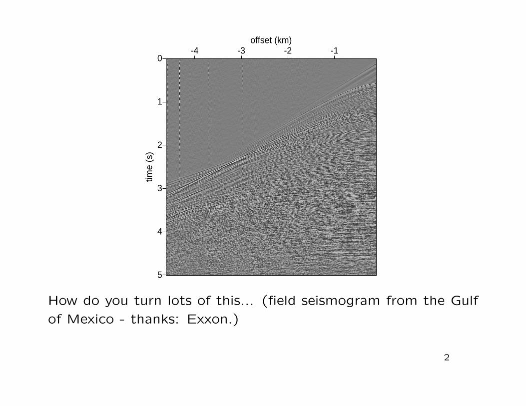
How do you turn lots of this... (field seismogram from the Gulf

of Mexico - thanks: Exxon.)

2

0

500

1000

1500

2000

2500

Depth

in M

ete

rs

0 200 400 600 800 1000 1200 1400CDP

into this (a fair rendition of subsurface structure)?

3

Central Point of These Talks:

Estimating the index of refraction (wave velocity) is the central

issue in seismic imaging.

Combines elements of

• optics, radar, sonar - reflected wave imaging

• tomography - with curved rays

Many unanswered mathematical questions with practical impli-

cations!4

A mathematical view of reflection seismic imaging, as practiced

in the petroleum industry:

• an inverse problem, based on a model of seismic wave prop-

agation

• contemporary practice relies on partial linearization and high-

frequency asymptotics

• recent progress in understanding capabilities, limitations of

methods based on linearization/asymptotics in presence of

strong refraction: applications of microlocal analysis with

implications for practice

• limitations of linearization lead to many open problems

5

Agenda

1. Seismic inverse problem in the acoustic model: nature of dataand model, linearization, reflectors and reflections idealizedvia harmonic analysis of singularities.

2. High frequency asymptotics: why adjoints of modeling oper-ators are imaging operators (“Kirchhoff migration”). Beylkintheory of high frequency asymptotic inversion.

3. Adjoint state imaging with the wave equation: reverse timeand reverse depth.

4. Geometric optics, Rakesh’s construction, and asymptotic in-version w/ caustics and multipathing.

5. A step beyond linearization: a mathematical framework forvelocity analysis, imaging artifacts, and prestack migrationapres Claerbout.

6

1. The Acoustic Model and Linearization

7

Marine reflection seismology apparatus:

• acoustic source (airgun array, explosives,...)

• acoustic receivers (hydrophone streamer, ocean bottom ca-ble,...)

• recording and onboard processing

Land acquisition similar, but acquisition and processing are morecomplex. Vast bulk (90%+) of data acquired each year is marine.

Data parameters: time t, source location xs, and receiver loca-tion xr or half offset h = xr−xs

2 , h = |h|.8

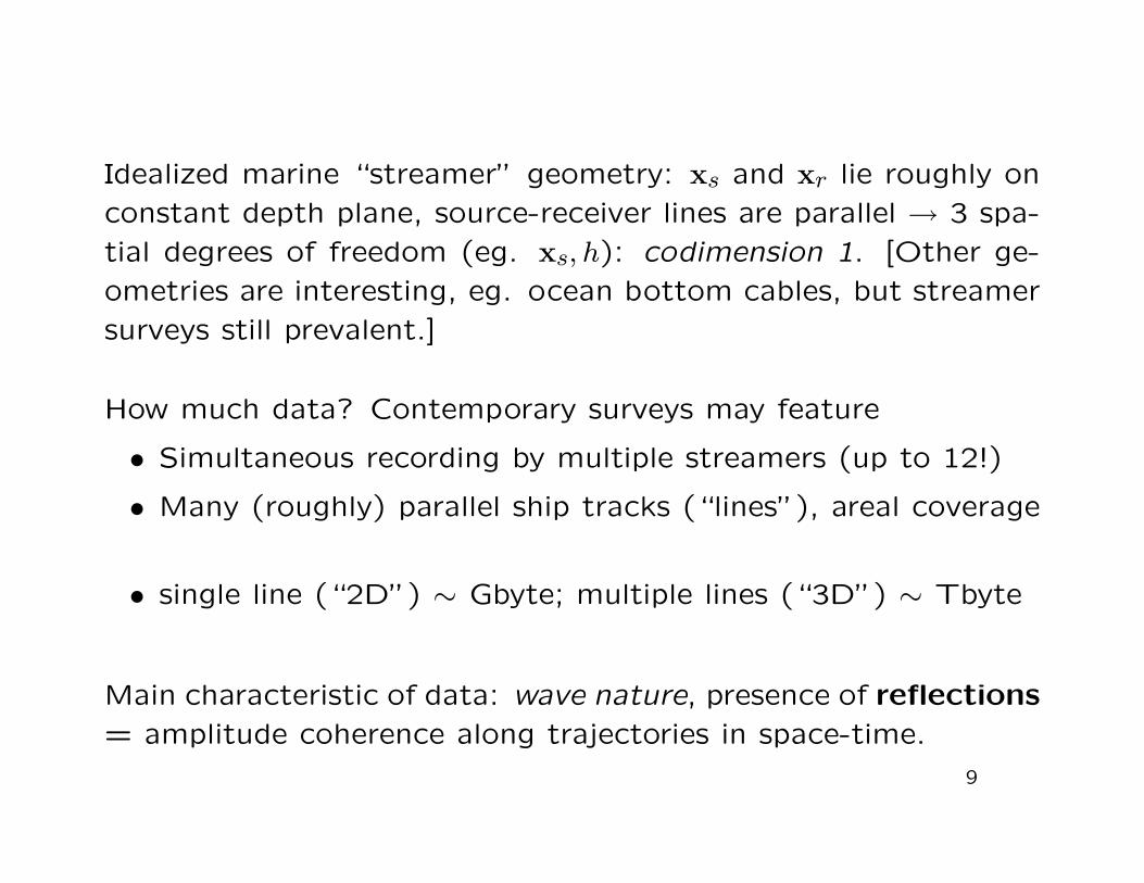
Idealized marine “streamer” geometry: xs and xr lie roughly on

constant depth plane, source-receiver lines are parallel → 3 spa-

tial degrees of freedom (eg. xs, h): codimension 1. [Other ge-

ometries are interesting, eg. ocean bottom cables, but streamer

surveys still prevalent.]

How much data? Contemporary surveys may feature

• Simultaneous recording by multiple streamers (up to 12!)

• Many (roughly) parallel ship tracks (“lines”), areal coverage

• single line (“2D”) ∼ Gbyte; multiple lines (“3D”) ∼ Tbyte

Main characteristic of data: wave nature, presence of reflections

= amplitude coherence along trajectories in space-time.

9

0

1

2

3

4

5

time

(s)

-4 -3 -2 -1offset (km)

Data from one source firing, Gulf of Mexico (thanks: Exxon)

10

1.0

1.5

2.0

2.5

3.0

-2.5 -2.0 -1.5 -1.0 -0.5

Lightly processed version of data displayed in previous slide -

bandpass filtered (in t), truncated (“muted”).

11

Distinguished data subsets: “gathers”, “bins”, extracted from

data after acquisition.

Characterized by common value of an acquisition parameter

• shot (or common source) gather: traces with same shot

location xs (previous expls)

• offset (or common offset) gather: traces with same half off-

set h

• ...

12

• presence of wave events (“reflections”) = coherent space-

time structures - clear from examination of the data.

• what features in the subsurface structure could cause reflec-

tions to occur?

13

1000 1200 1400 1600 1800 2000 2200 2400 2600 2800 3000500

1000

1500

2000

2500

3000

3500

4000

4500

depth (m)

Blocked logs from well in North Sea (thanks: Mobil R & D).

Solid: p-wave velocity (m/s), dashed: s-wave velocity (m/s),

dash-dot: density (kg/m3). “Blocked” means “averaged” (over

30 m windows). Original sample rate of log tool < 1 m. Re-

flectors = jumps in velocities, density, velocity trends.

14

Known that abrupt (wavelength scale) changes in material me-

chanics, i.e. reflectors, act as internal boundary, causing reflec-

tion of waves.

What is the mechanism through which this occurs?

Seek a simple model which quantitatively explains wave reflection

and other known features of the Earth’s interior.

15

The Modeling Task: any model of the reflection seismogrammust

• predict wave motion

• produce reflections from reflectors

• accomodate significant variation of wave velocity, materialdensity,...

A really good model will also accomodate

• multiple wave modes, speeds

• material anisotropy

• attenuation, frequency dispersion of waves

• complex source, receiver characteristics

16

Acoustic Model (only compressional waves)

Not really good, but good enough for today and basis of most

contemporary processing.

Relates ρ(x)= material density, λ(x) = bulk modulus, p(x, t)=

pressure, v(x, t) = particle velocity, f(x, t)= force density (sound

source):

ρ∂v

∂t= −∇p+ f ,

∂p

∂t= −λ∇ · v (+ i.c.′s,b.c.′s)

(compressional) wave speed c =√λρ

17

acoustic field potential u(x, t) =∫ t−∞ ds p(x, s):

p =∂u

∂t, v =

1

ρ∇u

Equivalent form: second order wave equation for potential

1

ρc2∂2u

∂t2−∇ ·

1

ρ∇u =

∫ t−∞

dt∇ ·(

f

ρ

)≡f

ρ

plus initial, boundary conditions.

18

Weak solution of Dirichlet problem in Ω ⊂ R3 (similar treatment

for other b. c.’s):

u ∈ C1([0, T ];L2(Ω)) ∩ C0([0, T ];H10(Ω))

satisfying for any φ ∈ C∞0 ((0, T )×Ω),∫ T0

∫Ωdt dx

1

ρc2∂u

∂t

∂φ

∂t−

1

ρ∇u · ∇φ+

1

ρfφ

= 0

Theorem (Lions, 1972) Suppose that log ρ, log c ∈ L∞(Ω), f ∈L2(Ω×R). Then weak solutions of Dirichlet problem exist; initial

data

u(·,0) ∈ H10(Ω),

∂u

∂t(·,0) ∈ L2(Ω)

uniquely determine them.

19

Further idealizations: (i) density is constant, (ii) source force

density is isotropic point radiator with known time dependence

(“source pulse” w(t))

f(x, t;xs) = w(t)δ(x− xs)

⇒ acoustic potential, pressure depends on xs also.

Example: numerical solution of 2D wave equation via finite dif-

ference method (2nd order in time, 4th order in space).

Model = velocity as function of position (in R2) = sum of

smooth trend plus zero mean fluctuations, both functions of

depth only. Source wavelet = bandpass filter.

20

0 200 400 600 800 1000 1200 1400 1600 1800 20001.5

1.55

1.6

1.65

1.7

1.75

1.8

1.85

1.9

1.95

depth (m)

veloci

ty (m/m

s)

Smooth trend of velocity.

21

0 200 400 600 800 1000 1200 1400 1600 1800 2000−0.15

−0.1

−0.05

0

0.05

0.1

0.15

0.2

0.25

0.3

0.35

depth (m)

Zero-mean fluctuations of velocity.

22

0 50 100 150 200 250 300−15

−10

−5

0

5

10

15

20

25

30

35

time (ms)

4-10-25-35 Hz bandpass filter, used as source wavelet.

23

ïÿØ|

1

10 20 30 40

1

10 20 30 40

0

1000

1950

100

200

300

400

500

600

700

800

900

1100

1200

1300

1400

1500

1600

1700

1800

1900

0

1000

1950

100

200

300

400

500

600

700

800

900

1100

1200

1300

1400

1500

1600

1700

1800

1900

Plane

Trace

Plane

Trace

Shot (common source) gather or bin, computed by finite differ-

ence simulation.

24

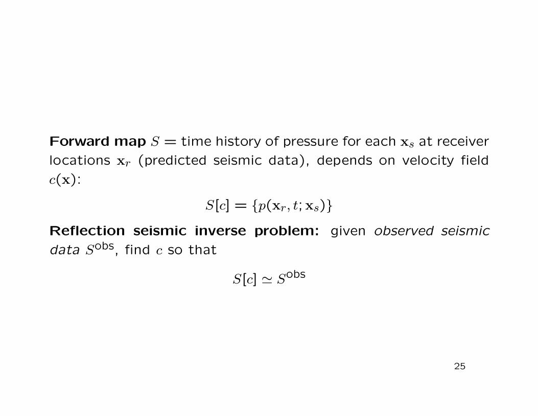
Forward map S = time history of pressure for each xs at receiver

locations xr (predicted seismic data), depends on velocity field

c(x):

S[c] = p(xr, t;xs)

Reflection seismic inverse problem: given observed seismic

data Sobs, find c so that

S[c] ' Sobs

25

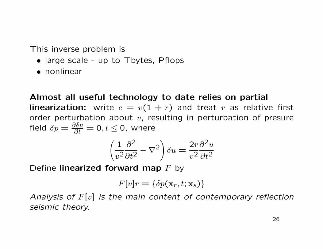
This inverse problem is

• large scale - up to Tbytes, Pflops

• nonlinear

Almost all useful technology to date relies on partiallinearization: write c = v(1 + r) and treat r as relative firstorder perturbation about v, resulting in perturbation of presurefield δp = ∂δu

∂t = 0, t ≤ 0, where(1

v2∂2

∂t2−∇2

)δu =

2r

v2∂2u

∂t2

Define linearized forward map F by

F [v]r = δp(xr, t;xs)Analysis of F [v] is the main content of contemporary reflectionseismic theory.

26

Critical question: If there is any justice F [v]r = derivative DS[v][vr]

of S - but in what sense? Physical intuition, numerical simula-

tion, and not nearly enough mathematics: linearization error

S[v(1 + r)]− (S[v] + F [v]r)

• small when v smooth, r rough or oscillatory on wavelength

scale - well-separated scales

• large when v not smooth and/or r not oscillatory - poorly

separated scales

2D finite difference simulation: shot gathers with typical marine

seismic geometry. Smooth (linear) v(x, z), oscillatory (random)

r(xz) depending only on z(“layered medium”)

27

0

0.2

0.4

0.6

0.8

1.0

z (k

m)

0 0.5 1.0 1.5 2.0x (km)

1.6

1.8

2.0

2.2

2.4

,

0

0.2

0.4

0.6

0.8

t (s)

0 0.2 0.4 0.6 0.8 1.0x_r (km)

Left: Smooth (linear) background v(x, z), oscillatory (random)

r(x, z). Std dev of r = 5%.

Right: Simulated seismic response (S[v(1+r)]), wavelet = band-

pass filter 4-10-30-45 Hz. Simulator is (2,4) finite difference

scheme.28

0

0.2

0.4

0.6

0.8

1.0

z (k

m)

0 0.5 1.0 1.5 2.0x (km)

1.6

1.8

2.0

2.2

2.4

,

0

0.2

0.4

0.6

0.8

1.0

z (k

m)

0 0.5 1.0 1.5 2.0x (km)

-0.10

-0.05

0

0.05

0.10

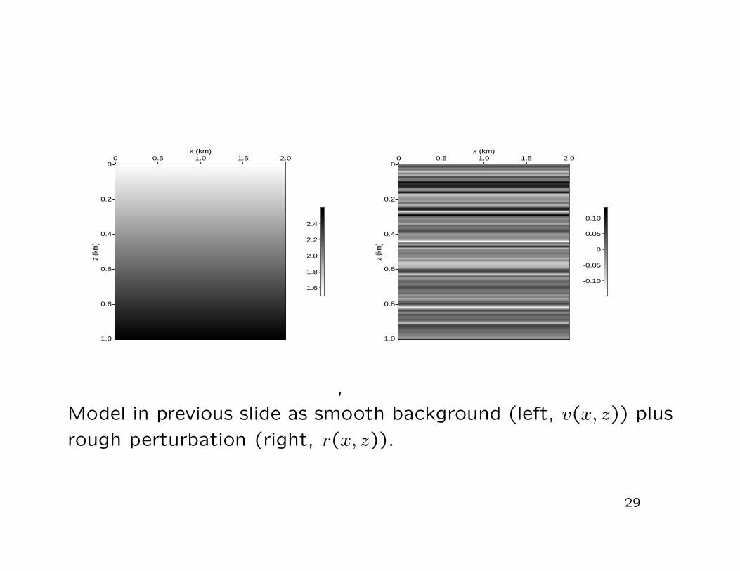
Model in previous slide as smooth background (left, v(x, z)) plus

rough perturbation (right, r(x, z)).

29

0

0.2

0.4

0.6

0.8

t (s)

0 0.2 0.4 0.6 0.8 1.0x_r (km)

.

0

0.2

0.4

0.6

0.8

t (s)

0 0.2 0.4 0.6 0.8 1.0x_r (km)

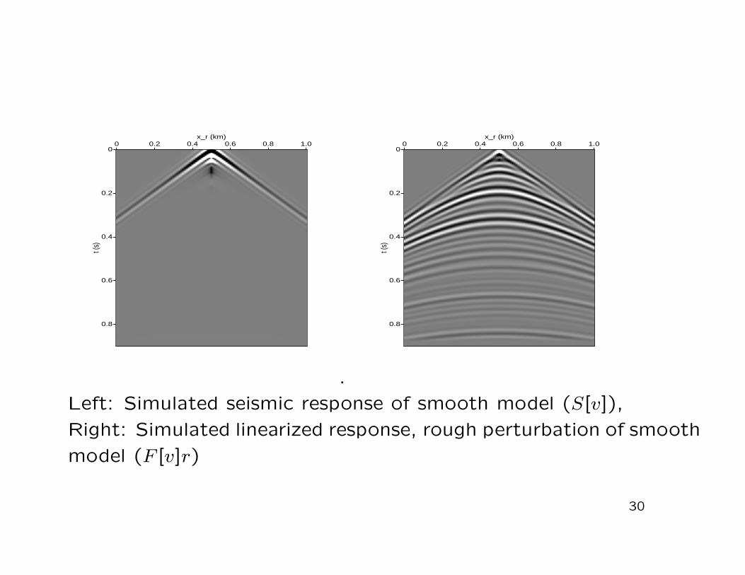
Left: Simulated seismic response of smooth model (S[v]),

Right: Simulated linearized response, rough perturbation of smooth

model (F [v]r)

30

0

0.2

0.4

0.6

0.8

1.0

z (k

m)

0 0.5 1.0 1.5 2.0x (km)

1.4

1.6

1.8

2.0

2.2

2.4

,

0

0.2

0.4

0.6

0.8

1.0

z (k

m)

0 0.5 1.0 1.5 2.0x (km)

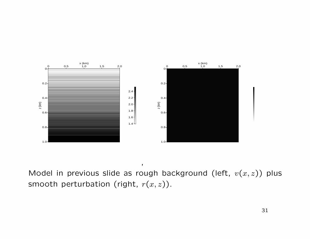
Model in previous slide as rough background (left, v(x, z)) plus

smooth perturbation (right, r(x, z)).

31

0

0.2

0.4

0.6

0.8

t (s)

0 0.2 0.4 0.6 0.8 1.0x_r (km)

.

0

0.2

0.4

0.6

0.8

t (s)

0 0.2 0.4 0.6 0.8 1.0x_r (km)

Left: Simulated seismic response of rough model (S[v]),

Right: Simulated linearized response, smooth perturbation of

rough model (F [v]r)

32

0

0.2

0.4

0.6

0.8

t (s)

0 0.2 0.4 0.6 0.8 1.0x_r (km)

,

0

0.2

0.4

0.6

0.8

t (s)

0 0.2 0.4 0.6 0.8 1.0x_r (km)

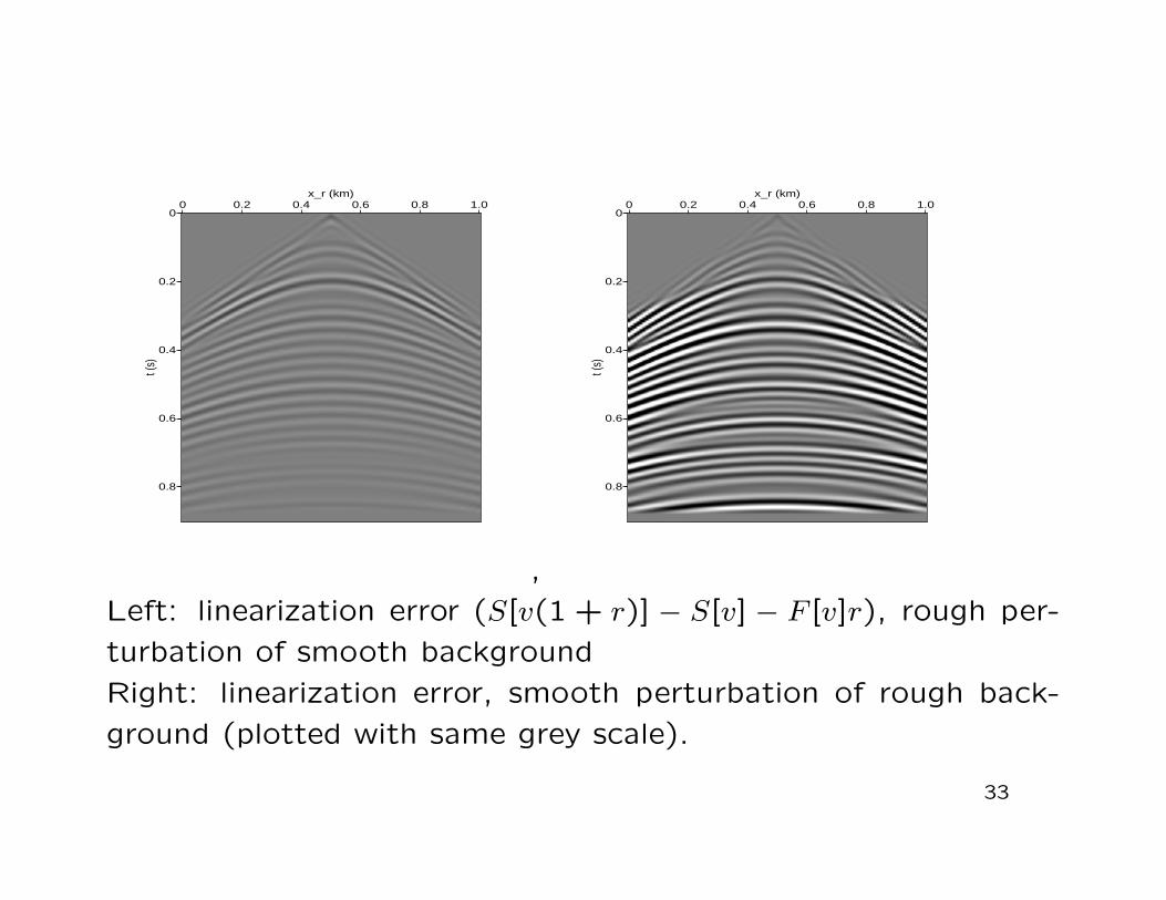
Left: linearization error (S[v(1 + r)] − S[v] − F [v]r), rough per-

turbation of smooth background

Right: linearization error, smooth perturbation of rough back-

ground (plotted with same grey scale).

33

Implications:

• Some geologies have well-separated scales - cf. sonic logs -

linearization-based methods work well there. Other geologies

do not - expect trouble!

• v smooth, r oscillatory ⇒ F [v]r approximates primary reflec-

tion = result of wave interacting with material heterogeneity

only once (single scattering); error consists of multiple re-

flections, which are “not too large” if r is “not too big”,

and sometimes can be suppressed (lecture 4).

• v nonsmooth, r smooth ⇒ error consists of time shifts in

waves which are very large perturbations as waves are oscil-

latory.

No mathematical results are known which justify/explain these

observations in any rigorous way.

34

Partially linearized inverse problem = velocity analysis problem:given Sobs find v, r so that

S[v] + F [v]r ' Sobs

Linear subproblem = imaging problem: given Sobs and v, findr so that

F [v]r ' Sobs − S[v]

Last 20 years:

• much progress on imaging problem

• much less on velocity analysis problem.

35

2. High frequency asymptotics and imaging operators

36

Importance of high frequency asymptotics: when linearization

is accurate, properties of F [v] dominated by those of Fδ[v] (=

F [v] with w = δ). Implicit in migration concept (eg. Hagedoorn,

1954); explicit use: Cohen & Bleistein, SIAM JAM 1977.

Key idea: reflectors (rapid changes in r) emulate singularities;

reflections (rapidly oscillating features in data) also emulate

singularities.

NB: “everybody’s favorite reflector”: the smooth interface across

which r jumps. But this is an oversimplification - reflectors in

the Earth may be complex zones of rapid change, pehaps in all

directions. More flexible notion needed!!

37

Paley-Wiener characterization of smoothness: u ∈ D′(Rn) is

smooth at x0 ⇔ can choose φ ∈ D(Rn) with φ(x0) 6= 0 so that

for any N , there is CN ≥ 0 so that for any ξ 6= 0,

|F(φu)(τξ)| ≤ CN(τ |ξ|)−N , all τ > 0

Harmonic analysis of singularities, apres Hormander: the wave

front set WF (u) ⊂ Rn ×Rn − 0 of u ∈ D′(Rn) - captures orien-

tation as well as position of singularities.

(x0, ξ0) /∈ WF (u) ⇔ can choose φ ∈ D(Rn) with φ(x0) 6= 0 and

an open nbhd Ξ ⊂ Rn−0 of ξ0 so that for any N , there is CN ≥ 0

so that for all ξ ∈ Ξ,

|F(φu)(τξ)| ≤ CN(τ |ξ|)−N , all τ > 0

38

Housekeeping chores:

(i) note that the nbhds Ξ may naturally be taken to be cones

(ii) WF (u) is invariant under chg. of coords if it is regarded as a

subset of the cotangent bundle T ∗(Rn) (i.e. the ξ components

transform as covectors).

[Good refs: Duistermaat, 1996; Taylor, 1981; Hormander, 1983]

The standard example: if u jumps across the interface f(x) =

0, otherwise smooth, then WF (u) ⊂ Nf = (x, ξ) : f(x) =

0, ξ||∇f(x) (normal bundle of f = 0).

39

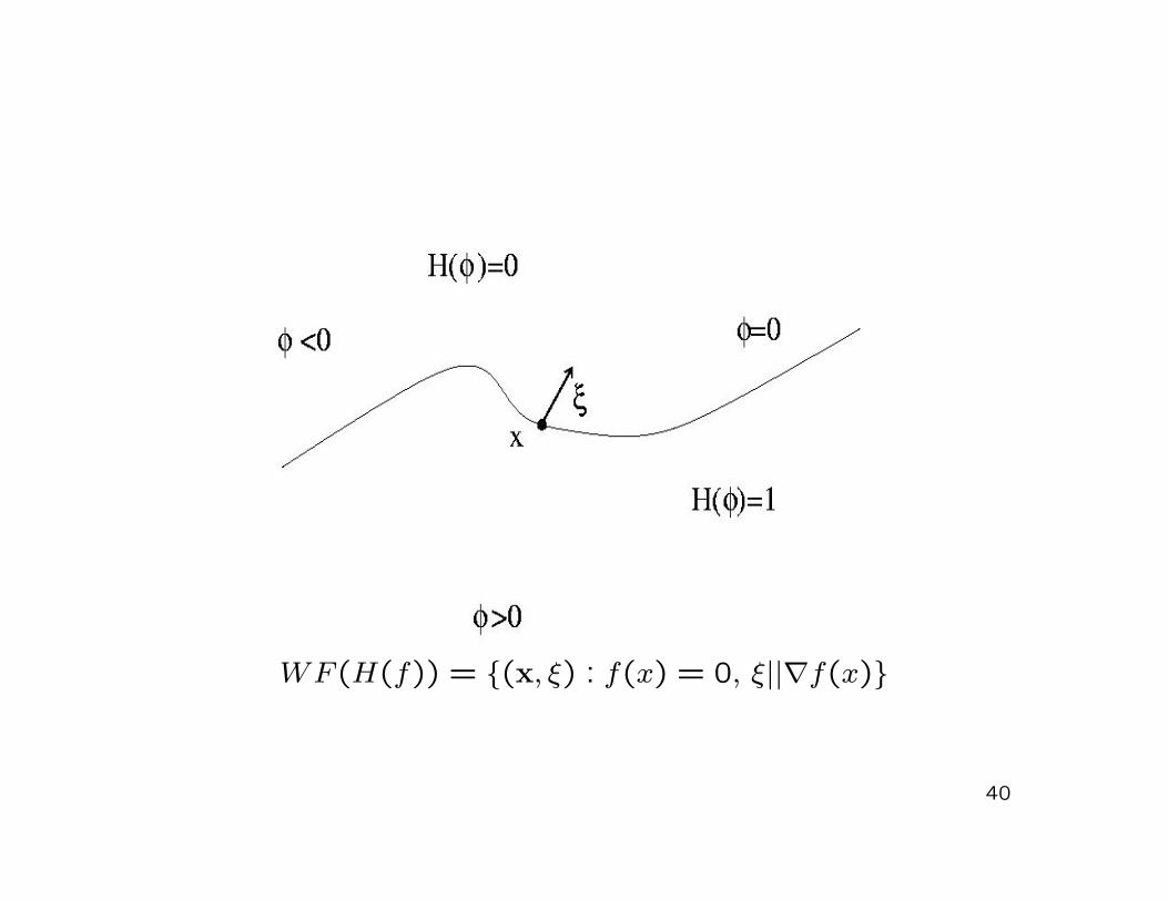
WF (H(f)) = (x, ξ) : f(x) = 0, ξ||∇f(x)

40

Fact (“microlocal property of differential operators”):

Suppose u ∈ D′(Rn), (x0, ξ0) /∈ WF (u), and P (x, D) is a partial

differential operator:

P (x, D) =∑

|α|≤maα(x)D

α

D = (D1, ..., Dn), Di = −i∂

∂xi

α = (α1, ..., αn), |α| =∑i

αi,

Dα = Dα11 ...Dαn

n

Then (x0, ξ0) /∈WF (P (x, D)u) [i.e.: WF (Pu) ⊂WF (u)].

41

Proof: Choose φ ∈ D, Ξ as in the definition, form the required

Fourier transform ∫dx eix·(τξ)φ(x)P (x, D)u(x)

and start integrating by parts: eventually

=∑

|α|≤mτ |α|ξα

∫dx eix·(τξ)φα(x)u(x)

where φα ∈ D is a linear combination of derivatives of φ and the

aαs. Since each integral is rapidly decreasing as τ →∞ for ξ ∈ Ξ,

it remains rapidly decreasing after multiplication by τ |α|, and so

does the sum. Q. E. D.

42

Key idea, restated: reflectors (or “reflecting elements”) will be

points in WF (r). Reflections will be points in WF (d).

These ideas lead to a usable definition of image: a reflectivity

model r is an image of r if WF (r) ⊂ WF (r) (the closer to

equality, the better the image).

Idealized migration problem: given d (hence WF (d)) deduce

somehow a function which has the right reflectors, i.e. a function

r with WF (r) 'WF (r).

NB: you’re going to need v! (“It all depends on v(x,y,z)” - J.

Claerbout)

43

With w = δ, acoustic potential u is same as Causal Green’s

function G(x, t;xs) = retarded fundamental solution:(1

v2∂2

∂t2−∇2

)G(x, t;xs) = δ(t)δ(x− bxs)

and G ≡ 0, t < 0. Then (w = δ!) p = ∂G∂t , δp = ∂δG

∂t , and(1

v2∂2

∂t2−∇2

)δG(x, t;xs) =

2

v2(x)

∂2G

∂t2(x, t;xs)r(x)

Simplification: from now on, define F [v]r = δG|x=xr - i.e. lose a

t-derivative. Duhamel’s principle ⇒

δG(xr, t;xs) =∫dx

2r(x)

v(x)2

∫dsG(xr, t− s;x)

∂2G

∂t2(x, s;xs)

44

Geometric optics approximation of G should be good, as v issmooth. Local version: if x “not too far” from xs, then

G(x, t;xs) = a(x;xs)δ(t− τ(x;xs)) +R(x, t;xs)

where the traveltime τ(x;xs) solves the eikonal equation

v|∇τ | = 1

τ(x;xs) ∼|x− xs|v(xs)

, x → xs

and the amplitude a(x;xs) solves the transport equation

∇ · (a2∇τ) = 0

All of this is meaningful only if the remainder R is small in asuitable sense: energy estimate (Exercise!) ⇒∫

dx∫ T0

dt |R(x, t;xs)|2 ≤ C‖v‖C4

45

Numerical solution of eikonal, transport: ray tracing (Lagrangian),

various sorts of upwind finite difference (Eulerian) methods. See

Sethian lectures, WWS 1999 MGSS notes (online) for details.

“Not too far” means: there should be one and only one ray of

geometric optics connecting each xs or xr to each x ∈ suppr.

For “random but smooth” v(x) with variance σ, more than one

connecting ray occurs as soon as the distance is O(σ−2/3). Such

multipathing is invariably accompanied by the formation of a

caustic (White, 1982).

Upon caustic formation, the simple geometric optics field de-

scription above is no longer correct (Ludwig, 1966).

46

0 0.1 0.2 0.3 0.4 0.5 0.6 0.7 0.8 0.9 1

0

0.2

0.4

0.6

0.8

1

1.2

1.4

1.6

1.8

2

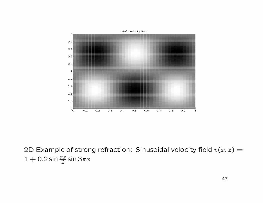
sin1: velocity field

2D Example of strong refraction: Sinusoidal velocity field v(x, z) =

1 + 0.2 sin πz2 sin 3πx

47

0 0.1 0.2 0.3 0.4 0.5 0.6 0.7 0.8 0.9 1

0

0.2

0.4

0.6

0.8

1

1.2

1.4

1.6

1.8

2

sin1: rays with takeoff angles in range 1.41372 to 1.72788

Rays in sinusoidal velocity field, source point = origin. Note for-

mation of caustic, multiple rays to source point in lower center.

48

Assume: supp r contained in simple geometric optics domain(each point reached by unique ray from any source point xs).

Then distribution kernel K of F [v] is

K(xr, t,xs;x) =∫dsG(xr, t− s;x)

∂2G

∂t2(x, s;xs)

2

v2(x)

'∫ds

2a(xr,x)a(x,xs)

v2(x)δ′(t− s− τ(xr,x))δ′′(s− τ(x,xs))

=2a(x,xr)a(x,xs)

v2(x)δ′′(t− τ(x,xr)− τ(x,xs))

provided that ∇xτ(x,xr)+∇xτ(x,xs) 6= 0 ⇔ velocity at x of rayfrom xs not negative of velocity of ray from xr ⇔ no forwardscattering. [Gel’fand and Shilov, 1958 - when is pullback ofdistribution again a distribution].

49

Q: What does ' mean?

A: It means “differs by something smoother”.

In theory, can complete the geometric optics approximation of

the Green’s function so that the difference is C∞ - then the two

sides have the same singularities, ie. the same wavefront set.

In practice, it’s sufficient to make the difference just a bit smoother,

so the first term of the geometric optics approximation (displayed

above) suffices (can formalize this with modification of wavefront

set defn).

These lectures will ignore the distinction.

50

So: for r supported in simple geometric optics domain, no for-

ward scattering ⇒

δG(xr, t;xs) '

∂2

∂t2

∫dx

2r(x)

v2(x)a(x,xr)a(x,xs)δ(t− τ(x,xr)− τ(x,xs))

That is: pressure perturbation is sum (integral) of r over re-

flection isochron x : t = τ(x,xr) + τ(x,xs), w. weighting,

filtering. Note: if v =const. then isochron is ellipsoid, as

τ(xs,x) = |xs − x|/v!

(y,x )+ (y,x )ττt=

x x

y

s

r s

r

51

1

20 30 40

1

20 30 40

400

1000

1400

500

600

700

800

900

1100

1200

1300

400

1000

1400

500

600

700

800

900

1100

1200

1300

Plane

Trace

Plane

Trace

,

1

20 30 40

1

20 30 40

400

1000

1400

500

600

700

800

900

1100

1200

1300

400

1000

1400

500

600

700

800

900

1100

1200

1300

Plane

Trace

Plane

Trace

,

1

20 30 40

1

20 30 40

400

1000

1400

500

600

700

800

900

1100

1200

1300

400

1000

1400

500

600

700

800

900

1100

1200

1300

Plane

Trace

Plane

Trace

Left: FD linearized simulation of shot gather, (i.e. δG(xr, t;xs)for fixed xs, convolved with bandpass filter source wavelet).Middle: Detail of numerical implementation of geometric opticsapproximation.Right: Difference, plotted on same scale.

52

Zero Offset data and the Exploding Reflector

Zero offset data (xs = xr) is seldom actually measured (contrast

radar, sonar!), but routinely approximated through NMO-stack

(to be explained later).

Extracting image from zero offset data, rather than from all

(100’s) of offsets, is tremendous data reduction - when approx-

imation is accurate, leads to excellent images.

Imaging basis: the exploding reflector model (Claerbout, 1970’s).

53

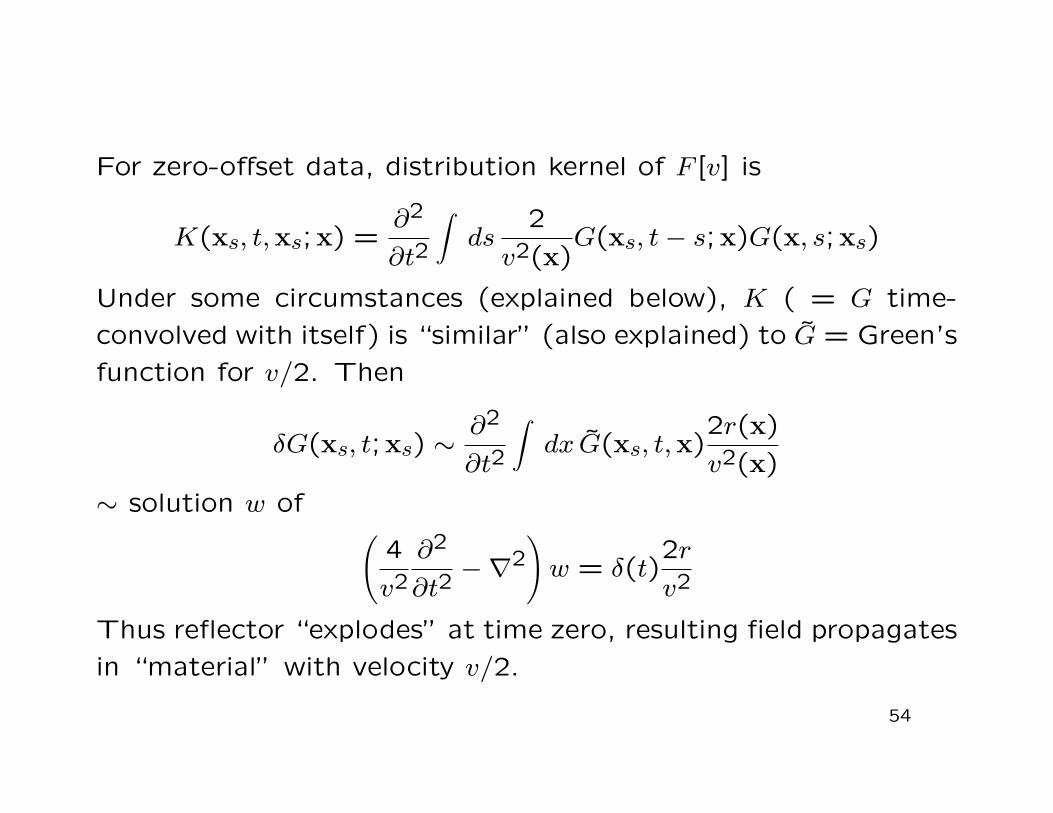
For zero-offset data, distribution kernel of F [v] is

K(xs, t,xs;x) =∂2

∂t2

∫ds

2

v2(x)G(xs, t− s;x)G(x, s;xs)

Under some circumstances (explained below), K ( = G time-

convolved with itself) is “similar” (also explained) to G = Green’s

function for v/2. Then

δG(xs, t;xs) ∼∂2

∂t2

∫dx G(xs, t,x)

2r(x)

v2(x)

∼ solution w of (4

v2∂2

∂t2−∇2

)w = δ(t)

2r

v2

Thus reflector “explodes” at time zero, resulting field propagates

in “material” with velocity v/2.

54

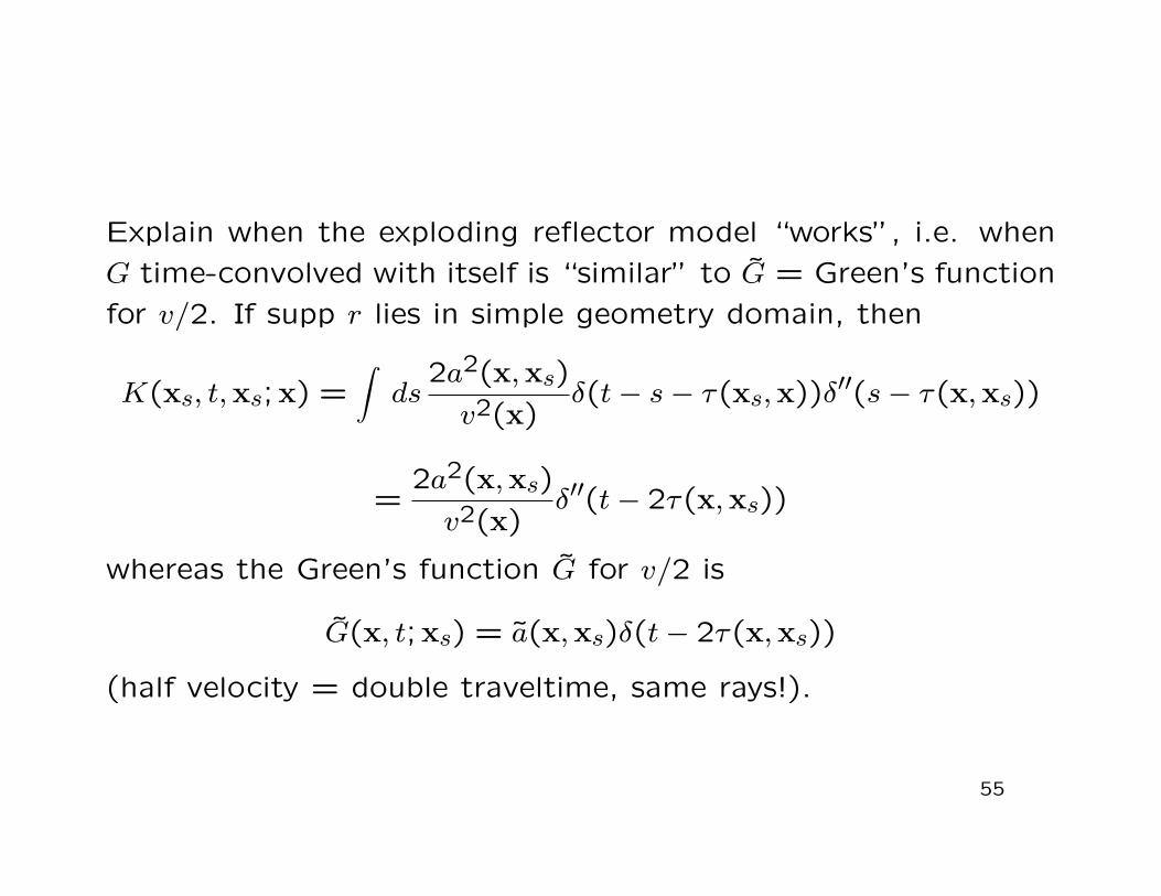
Explain when the exploding reflector model “works”, i.e. when

G time-convolved with itself is “similar” to G = Green’s function

for v/2. If supp r lies in simple geometry domain, then

K(xs, t,xs;x) =∫ds

2a2(x,xs)

v2(x)δ(t− s− τ(xs,x))δ′′(s− τ(x,xs))

=2a2(x,xs)

v2(x)δ′′(t− 2τ(x,xs))

whereas the Green’s function G for v/2 is

G(x, t;xs) = a(x,xs)δ(t− 2τ(x,xs))

(half velocity = double traveltime, same rays!).

55

Difference between effects of K, G: for each xs scale r by smooth

fcn - preserves WF (r) hence WF (F [v]r) and relation between

them. Also: adjoints have same effect on WF sets.

Upshot: from imaging point of view (i.e. apart from amplitude,

derivative (filter)), kernel of F [v] restricted to zero offset is same

as Green’s function for v/2, provided that simple geometry hy-

pothesis holds: only one ray connects each source point to each

scattering point, ie. no multipathing.

See Claerbout, BEI, for examples which demonstrate that mul-

tipathing really does invalidate exploding reflector model.

56

Standard Processing: an inspirational interlude

Suppose were v,r functions of z = x3 only, all sources and re-

ceivers at z = 0. Then the entire system is translation-invariant

in x1, x2 ⇒ Green’s function G its perturbation δG, and the ide-

alized data δG|z=0 are really only functions of t and half-offset

h = |xs − xr|/2. There would be only one seismic experiment,

equivalent to any common midpoint gather (“CMP”) = traces

with the same midpoint xm = (xr + xs)/2.

This isn’t really true - look at the data!!! However it is approxi-

mately correct in many places in the world: CMPs change slowly

with midpoint

57

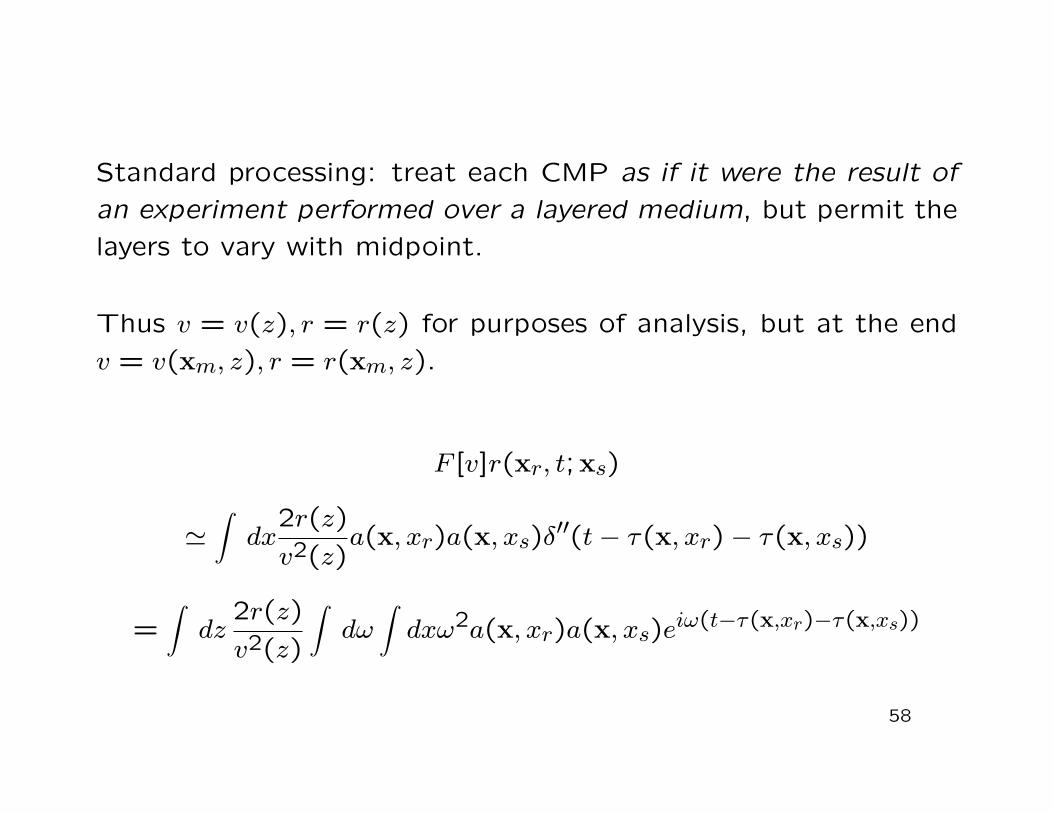
Standard processing: treat each CMP as if it were the result of

an experiment performed over a layered medium, but permit the

layers to vary with midpoint.

Thus v = v(z), r = r(z) for purposes of analysis, but at the end

v = v(xm, z), r = r(xm, z).

F [v]r(xr, t;xs)

'∫dx

2r(z)

v2(z)a(x, xr)a(x, xs)δ

′′(t− τ(x, xr)− τ(x, xs))

=∫dz

2r(z)

v2(z)

∫dω

∫dxω2a(x, xr)a(x, xs)e

iω(t−τ(x,xr)−τ(x,xs))

58

Since we have already thrown away smoother (lower frequency)

terms, do it again using stationary phase. Upshot (see 2000

MGSS notes for details): up to smoother (lower frequency) error,

F [v]r(h, t) ' A(z(h, t), h)R(z(h, t))

Here z(h, t) is the inverse of the 2-way traveltime

t(h, z) = 2τ((h,0, z), (0,0,0))

i.e. z(t(h, z′), h) = z′. R is (yet another version of) “reflectivity”

R(z) =1

2

dr

dz(z)

That is, F [v] is a a derivative followed by a change of variable

followed by multiplication by a smooth function. Substitute t0(vertical travel time) for z (depth) and you get “Inverse NMO”

(t0 → (t, h)). Will be sloppy and call z → (t, h) INMO.

59

0

0.2

0.4

0.6

0.8

1.0

t0 (

s)

1

,

0

0.2

0.4

0.6

0.8

1.0

t (s

)

0 1h (km)

,

0

0.2

0.4

0.6

0.8

1.0

t (s

)

0 1h (km)

Left: r(t0). Middle: r(ζ(t, h)). Right: F [v]r(t, h)

60

Anatomy of an adjoint:∫dt∫dh d(t, h)F [v]r(t, h) =

∫dt∫dh d(t, h)A(z(t, h), h)R(z(t, h))

=∫dz R(z)

∫dh

∂t

∂z(z, h)A(z, h)d(t(z, h), h) =

∫dz r(z)(F [v]∗d)(z)

so F [v]∗ = − ∂∂zSM [v]N [v],

N [v] = NMO operator N [v]d(z, h) = d(t(z, h), h)

M [v] = multiplication by ∂t∂zA

S = stacking operator

Sf(z) =∫dh f(z, h)

61

0

0.2

0.4

0.6

0.8

1.0

t (s

)

0 1h (km)

,

0

0.2

0.4

0.6

0.8

1.0

t0 (

s)

0 1h (km)

,

0

0.2

0.4

0.6

0.8

1.0

t0 (

s)

0 1h (km)

Left: d(t, h) = F [v]r(t, h). Middle: N [v]d(t0, h). Right:

N [v1]d(t0, h), v1 6= v

62

Stack as ersatz ZO section: how to ”get” ZO data even if youdon’t measure it.

If you use t0 instead of z to parametrize depth, and data isconsistent with conv. model, then

every trace looks exactly like the zero offset trace - even if youdon’t measure the zero offset trace!

Therefore stack = average of a bunch of traces (output of NMO)which have events in exactly the same place (t0) as ZO trace.Hence view stack as substitute for ZO data.

Adjusting velocity estimate to align NMO corrected traces pro-duces stacking velocity - if successful, then stack enhances signal,suppresses (coherent and incoherent) noise.

63

Imaging in standard processing: suppose that Sobs is model-

consistent, i.e. d ≡ Sobs − S[v] = F [v]r. Then

F [v]∗d = F [v]∗F [v]r(z)

= −∂

∂z

[∫dh

dt

dz(z, h)A2(z, h)

]∂

∂zr(z)

Microlocal property of PDOs ⇒ WF (F [v]∗F [v]r) ⊂ WF (r) i.e.

F [v]∗ is an imaging operator.

If you leave out the amplitude factor (M [v]) and the derivatives,

as is commonly done, then you get essentially the same expres-

sion - so (NMO, stack) is an imaging operator!

Now make everything dependent on xm and you’ve got standard

processing. (end of standard processing interlude).

64

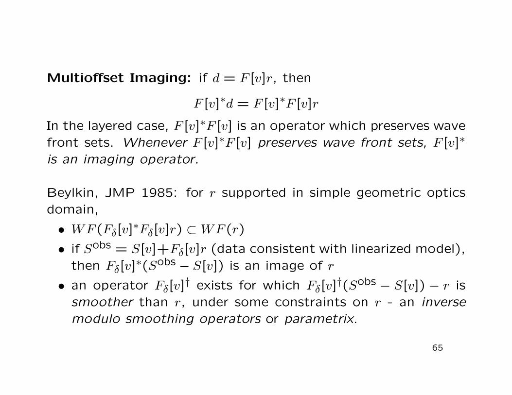
Multioffset Imaging: if d = F [v]r, then

F [v]∗d = F [v]∗F [v]r

In the layered case, F [v]∗F [v] is an operator which preserves wavefront sets. Whenever F [v]∗F [v] preserves wave front sets, F [v]∗

is an imaging operator.

Beylkin, JMP 1985: for r supported in simple geometric opticsdomain,

• WF (Fδ[v]∗Fδ[v]r) ⊂WF (r)

• if Sobs = S[v]+Fδ[v]r (data consistent with linearized model),then Fδ[v]

∗(Sobs − S[v]) is an image of r

• an operator Fδ[v]† exists for which Fδ[v]

†(Sobs − S[v]) − r issmoother than r, under some constraints on r - an inversemodulo smoothing operators or parametrix.

65

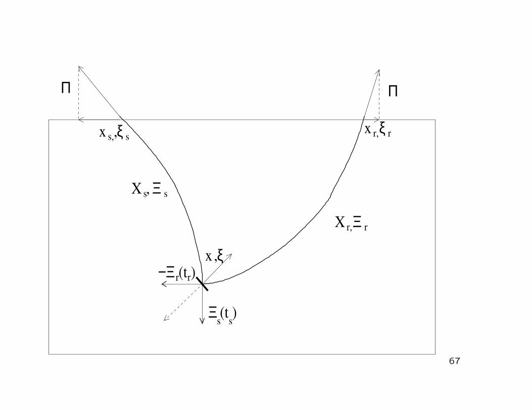
Also: explicit relation between WF (d) and WF (r) (”canonical

relation”).

(x, ξ) ∈WF (r) ⇔ (xs,xr, t, ξs, ξr, ω) ∈WF (d)

and (1) the source ray connects (xs, ξs) to (x,Ξs) with traveltime

τ(x,xs);

(2) the receiver ray connects (xr, ξr) to (x,Ξr) with traveltime

τ(x,xr);

(3) ξ‖Ξs + Ξr (”Snell’s law”);

(4) t = τ(x,xs) + τ(x,xr).

66

−Ξ

X

s

r

Ξ (t )s

r (t )

X s

x

x x ξ rs, r,sξ,

Ξ s

ξ,

rΞr,

,

ΠΠ

67

Outline of proof: (i) express F [v]∗F [v] as “Kirchhoff modeling”

followed by “Kirchhoff migration”; (ii) introduce Fourier trans-

form; (iii) approximate for large wavenumbers using stationary

phase, leads to representation of F [v]∗F [v] modulo smoothing

error as pseudodifferential operator (“ΨDO”):

F [v]∗F [v]r(x) ' p(x, D)r(x) ≡∫dξ p(x, ξ)eix·ξr(ξ)

in which p ∈ C∞, and for some m (the order of p), all multiindices

α, β, and all compact K ⊂ Rn, there exist constants Cα,β,K ≥ 0

for which

|DαxD

βξ p(x, ξ)| ≤ Cα,β,K(1 + |ξ|)m−|β|, x ∈ K

Explicit computation of symbol p - for details, .

68

Imaging property of Kirchhoff migration follows from microlocalproperty of ΨDOs:

if p(x,D) is a ΨDO, u ∈ E ′(Rn) then WF (p(x,D)u) ⊂WF (u).

Will prove this. First, a few other properties:

• differential operators are ΨDOs (easy - exercise)

• ΨDOs of order m form a module over C∞(Rn) (also easy)

• product of ΨDO order m, ΨDO order l = ΨDO order ≤ m+l;adjoint of ΨDO order m is ΨDO order m (much harder)

Complete accounts of theory, many apps: books of Duistermaat,Taylor, Nirenberg, Treves, Hormander.

69

Proof of microlocal property: suppose (x0, ξ0) /∈WF (u), choose

neighborhoods X, Ξ as in defn, with Ξ conic. Need to choose

analogous nbhds for P (x,D)u. Pick δ > 0 so that B3δ(x0) ⊂ X,

set X ′ = Bδ(x0).

Similarly pick 0 < ε < 1/3 so that B3ε(ξ0/|ξ0|) ⊂ Ξ, and chose

Ξ′ = τξ : ξ ∈ Bε(ξ0/|ξ0|), τ > 0.

Need to choose φ ∈ E ′(X ′), estimate F(φP (x, D)u). Choose

ψ ∈ E(X) so that ψ ≡ 1 on B2δ(x0).

NB: this implies that if x ∈ X ′, ψ(y) 6= 1 then |x− y| ≥ δ.

70

Write u = (1− ψ)u+ ψu. Claim: φP (x, D)((1− ψ)u) is smooth.

φ(x)P (x, D)((1− ψ)u))(x)

= φ(x)∫dξ P (x, ξ)eix·ξ

∫dy (1− ψ(y))u(y)e−iy·ξ

=∫dξ

∫dy P (x, ξ)φ(x)(1− ψ(y))ei(x−y)·ξu(y)

=∫dξ

∫dy (−∇2

ξ )MP (x, ξ)φ(x)(1−ψ(y))|x−y|−2Mei(x−y)·ξu(y)

using the identity

ei(x−y)·ξ = |x− y|−2[−∇2

ξ ei(x−y)·ξ

]and integrating by parts 2M times in ξ. This is permissible

because φ(x)(1− ψ(y)) 6= 0 ⇒ |x− y| > δ.

71

According to the definition of ΨDO,

|(−∇2ξ )MP (x, ξ)| ≤ C|ξ|m−2M

For any K, the integral thus becomes absolutely convergent after

K differentiations of the integrand, provided M is chosen large

enough. Q.E.D. Claim.

This leaves us with φP (x, D)(ψu). Pick η ∈ Ξ′ and w.l.o.g. scale

|η| = 1. Fourier transform:

F(φP (x, D)(ψu))(τη) =∫dx

∫dξ P (x, ξ)φ(x)ψu(ξ)eix·(ξ−τη)

Introduce τθ = ξ, and rewrite this as

= τn∫dx

∫dθ P (x, τθ)φ(x)ψu(τθ)eiτx·(θ−η)

72

Divide the domain of the inner integral into θ : |θ − η| > ε and

its complement. Use

−∇2xeiτx·(θ−η) = τ2|θ − η|2eiτx·(θ−η)

and integration by parts 2M times to estimate the first integral:

τn−2M

∣∣∣∣∣∫dx

∫|θ−η|>ε

dθ (−∇2x)M [P (x, τθ)φ(x)]ψu(τθ)

× |θ − η|−2Meiτx·(θ−η)∣∣∣

≤ Cτn+m−2M

m being the order of P . Thus the first integral is rapidly de-

creasing in τ .

73

For the second integral, note that |θ − η| ≤ ε ⇒ θ ∈ Ξ, per the

defn of Ξ′. Since X ×Ξ is disjoint from the wavefront set of u,

for a sequence of constants CN , |ψu(τθ)| ≤ CNτ−N uniformly for

θ in the (compact) domain of integration, whence the second

integral is also rapidly decreasing in τ . Q. E. D.

And that’s why Kirchhoff migration works, at least in the simple

geometric optics regime.

74

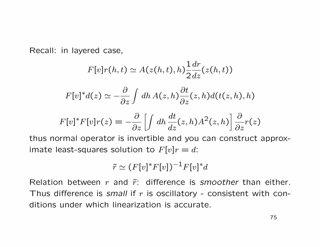
Recall: in layered case,

F [v]r(h, t) ' A(z(h, t), h)1

2

dr

dz(z(h, t))

F [v]∗d(z) ' −∂

∂z

∫dhA(z, h)

∂t

∂z(z, h)d(t(z, h), h)

F [v]∗F [v]r(z) = −∂

∂z

[∫dh

dt

dz(z, h)A2(z, h)

]∂

∂zr(z)

thus normal operator is invertible and you can construct approx-

imate least-squares solution to F [v]r = d:

r ' (F [v]∗F [v])−1F [v]∗d

Relation between r and r: difference is smoother than either.

Thus difference is small if r is oscillatory - consistent with con-

ditions under which linearization is accurate.

75

Analogous construction in simple geometric optics case: due to

Beylkin (1985).

Complication: F [v]∗F [v] cannot be invertible - becauseWF (F [v]∗F [v]r)

generally quite a bit smaller than WF (r).

Inversion aperture Γ[v] ⊂ R3 × R3 − 0: if WF (r) ⊂ Γ[v], then

WF (F [v]∗F [v]r) = WF (r) and F [v]∗F [v] “acts invertible”. [con-

struction of Γ[v] - later!]

Beylkin: with proper choice of amplitude b(xr, t;xs), the modified

Kirchhoff migration operator

F [v]†d(x) =∫ ∫ ∫

dxr dxs dt b(xr, t;xs)δ(t−τ(x;xs)−τ(x;xr))d(xr, t;xs)

yields F [v]†F [v]r ' r if WF (r) ⊂ Γ[v]

76

For details of Beylkin construction: Beylkin, 1985; Miller et al

1989; Bleistein, Cohen, and Stockwell 2000; WWS MGSS notes

1998. All components are by-products of eikonal solution.

aka: Generalized Radon Transform (“GRT”) inversion, Ray-

Born inversion, migration/inversion, true amplitude migration,...

Many extensions, eg. to elasticity: Bleistein, Burridge, deHoop,

Lambare,...

Apparent limitation: construction relies on simple geometric op-

tics (no multipathing) - how much of this can be rescued? cf.

Lecture 3.

77

0

500

1000

1500

2000

2500

Depth

in M

ete

rs

0 200 400 600 800 1000 1200 1400CDP

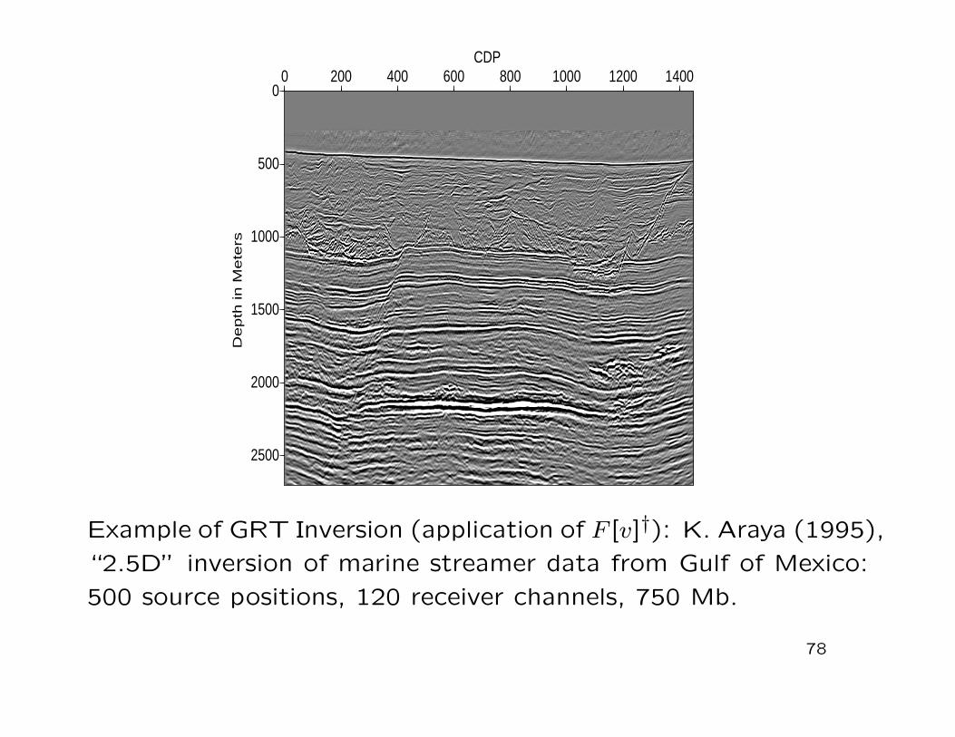
Example of GRT Inversion (application of F [v]†): K. Araya (1995),

“2.5D” inversion of marine streamer data from Gulf of Mexico:

500 source positions, 120 receiver channels, 750 Mb.

78