matheuristics for combinatorial optimization problems

MATHEURISTICS FOR COMBINATORIAL

OPTIMIZATION PROBLEMS

Module 1- Lesson 4

Prof. Maurizio Bruglieri

Politecnico di Milano

OUTLINE - Decomposition based matheur.

• Classification of decomposition based matheuristics (“natural” vs “artificial” decomposition)

• Decomposition based matheuristics for the VRP:➢ Generalized Assignment heuristic➢ Location heuristic➢ Route-first, cluster-second heuristic

• Lagrangean decomposition matheuristic➢ Application to hazmat transport

• Dantzig-Wolfe decomposition matheuristic

2

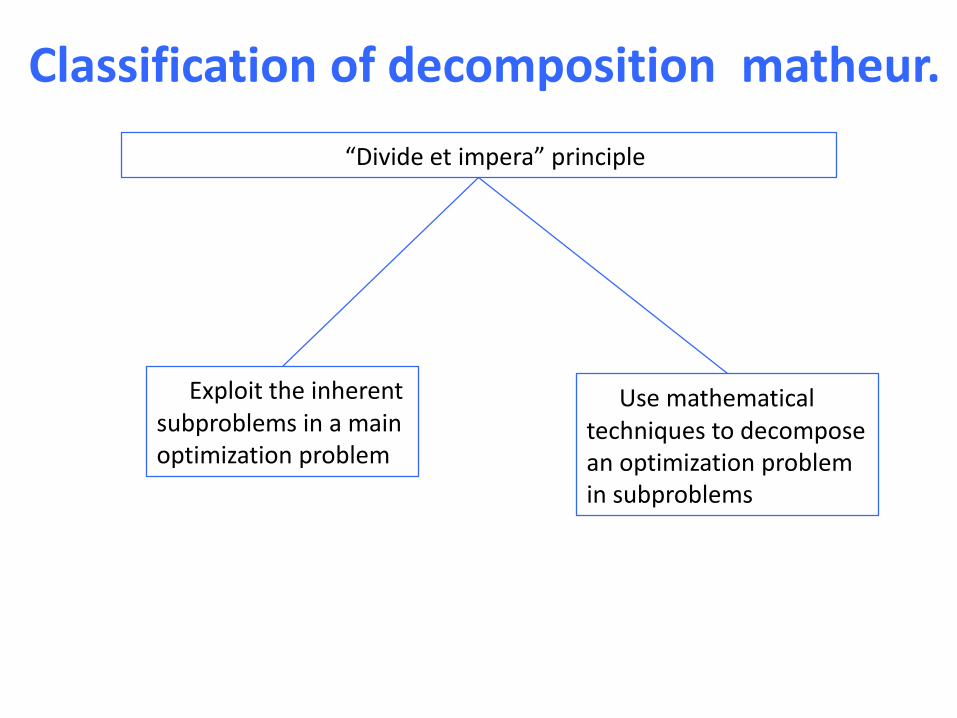
Classification of decomposition matheur.

“Divide et impera” principle

Exploit the inherentsubproblems in a main optimization problem

Use mathematical techniques to decompose an optimization problem in subproblems

“Natural” decomposition matheuristics• Some optimization problems are naturally structured as a sequence

of optimization subproblems.

• In the airline crew and fleet planning:

• In the Vehicle Routing Problem (VRP):

→

routing of each vehicle (TSP)

assignment of customers to the vehicles

airline fleet planning passenger schedule crew pairing problem→ →airline fleet planning →

Decomposition matheuristics for VRP

𝑖

𝑞𝑖𝑥𝑖𝑗 ≤ 𝑄

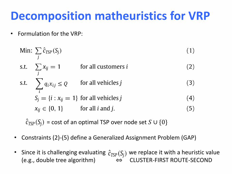
• Formulation for the VRP:

= cost of an optimal TSP over node set 𝑆 ∪ {0}

• Constraints (2)-(5) define a Generalized Assignment Problem (GAP)

• Since it is challenging evaluating we replace it with a heuristic value (e.g., double tree algorithm) ⇔ CLUSTER-FIRST ROUTE-SECOND

Generalized Assignment matheur. for VRP• Introduced by Fisher and Jaikumar (1981):

1. Choose seed nodes sj for j=1,…,m

2. Solve the GA: min σ𝑖𝑗 𝑐𝑖𝑠𝑗 𝑥𝑖𝑗: 2 − 5

3. Solve (heuristically) a TSP over each cluster 𝑆𝑗 ∪ 0 defined in step 2

• Drawback of this approach: its dependency on the seed selection step

• For this reason in the next heuristic, steps 1 and 2 are combined

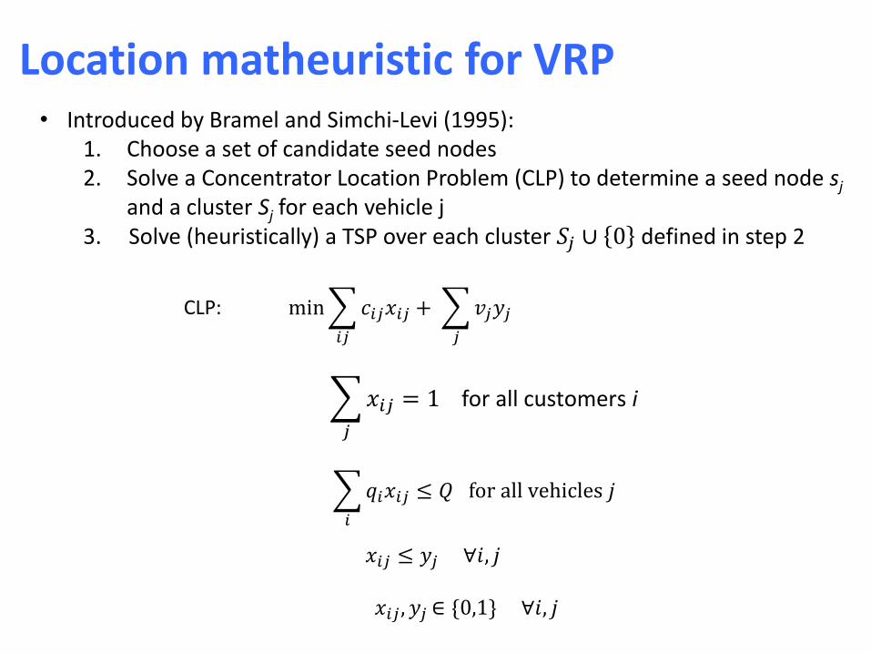
Location matheuristic for VRP• Introduced by Bramel and Simchi-Levi (1995):

1. Choose a set of candidate seed nodes2. Solve a Concentrator Location Problem (CLP) to determine a seed node sj

and a cluster Sj for each vehicle j3. Solve (heuristically) a TSP over each cluster 𝑆𝑗 ∪ 0 defined in step 2

min

𝑖𝑗

𝑐𝑖𝑗𝑥𝑖𝑗 +

𝑗

𝑣𝑗𝑦𝑗CLP:

𝑗

𝑥𝑖𝑗 = 1 for all customers i

𝑖

𝑞𝑖𝑥𝑖𝑗 ≤ 𝑄 for all vehicles 𝑗

𝑥𝑖𝑗 ≤ 𝑦𝑗 ∀𝑖, 𝑗

𝑥𝑖𝑗 , 𝑦𝑗 ∈ {0,1} ∀𝑖, 𝑗

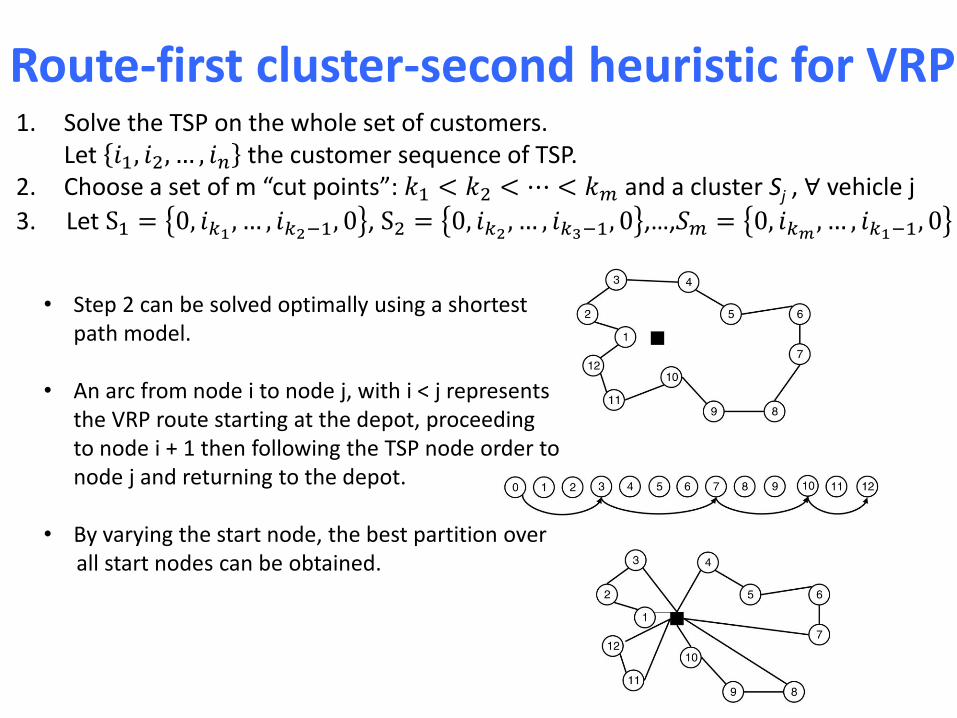
Route-first cluster-second heuristic for VRP1. Solve the TSP on the whole set of customers.

Let 𝑖1, 𝑖2, … , 𝑖𝑛 the customer sequence of TSP. 2. Choose a set of m “cut points”: 𝑘1 < 𝑘2 < ⋯ < 𝑘𝑚 and a cluster Sj , ∀ vehicle j

3. Let S1 = 0, 𝑖𝑘1 , … , 𝑖𝑘2−1, 0 , S2 = 0, 𝑖𝑘2 , … , 𝑖𝑘3−1, 0 ,…,𝑆𝑚 = 0, 𝑖𝑘𝑚 , … , 𝑖𝑘1−1, 0

• Step 2 can be solved optimally using a shortestpath model.

• An arc from node i to node j, with i < j representsthe VRP route starting at the depot, proceedingto node i + 1 then following the TSP node order to node j and returning to the depot.

• By varying the start node, the best partition overall start nodes can be obtained.

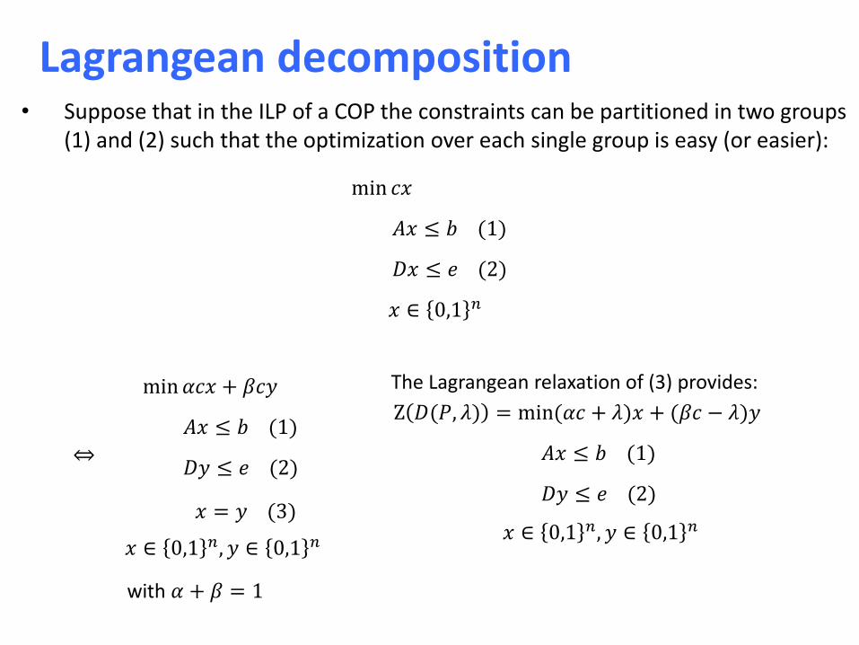
Lagrangean decomposition• Suppose that in the ILP of a COP the constraints can be partitioned in two groups

(1) and (2) such that the optimization over each single group is easy (or easier):

min 𝑐𝑥

𝐴𝑥 ≤ 𝑏 (1)

𝐷𝑥 ≤ 𝑒 (2)

𝑥 ∈ 0,1 𝑛

The Lagrangean relaxation of (3) provides:

Z 𝐷(𝑃, 𝜆) = min(𝛼𝑐 + 𝜆)𝑥 + (𝛽𝑐 − 𝜆)𝑦

𝐴𝑥 ≤ 𝑏 (1)

𝐷𝑦 ≤ 𝑒 (2)

𝑥 ∈ 0,1 𝑛, 𝑦 ∈ 0,1 𝑛

⇔

min𝛼𝑐𝑥 + 𝛽𝑐𝑦

𝐴𝑥 ≤ 𝑏 (1)

𝐷𝑦 ≤ 𝑒 (2)

𝑥 ∈ 0,1 𝑛, 𝑦 ∈ 0,1 𝑛

𝑥 = 𝑦 (3)

with 𝛼 + 𝛽 = 1

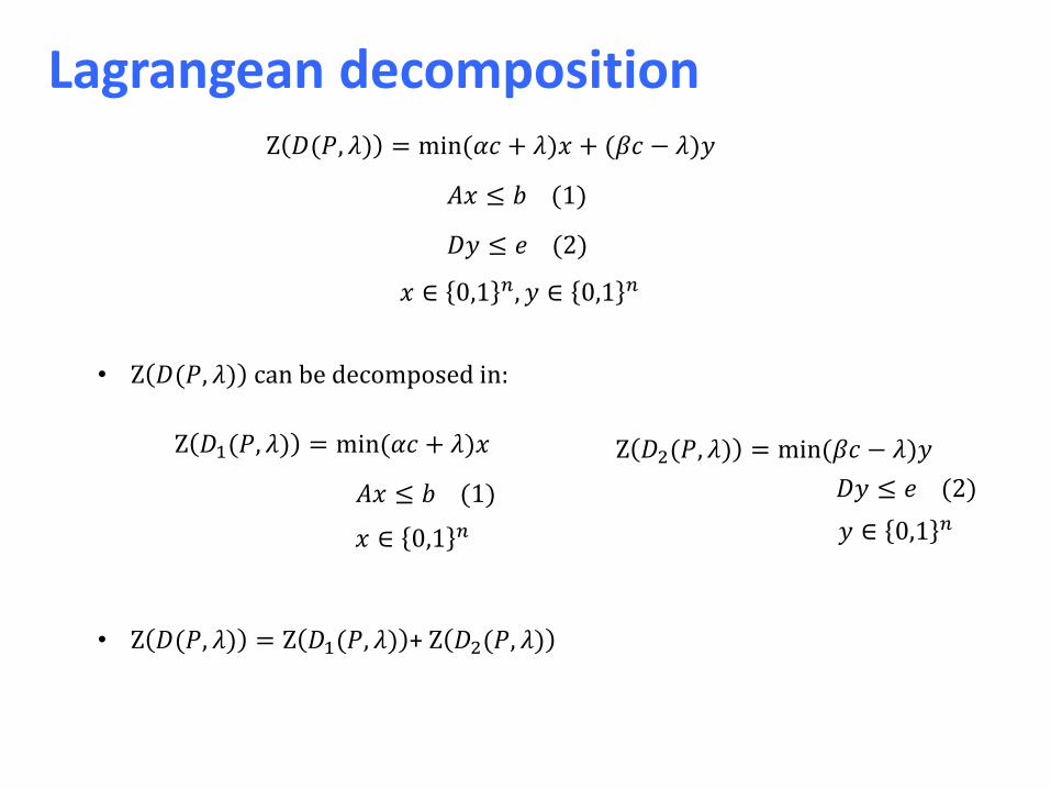
Lagrangean decompositionZ 𝐷(𝑃, 𝜆) = min(𝛼𝑐 + 𝜆)𝑥 + (𝛽𝑐 − 𝜆)𝑦

𝐴𝑥 ≤ 𝑏 (1)

𝐷𝑦 ≤ 𝑒 (2)

𝑥 ∈ 0,1 𝑛, 𝑦 ∈ 0,1 𝑛

Z 𝐷1(𝑃, 𝜆) = min(𝛼𝑐 + 𝜆)𝑥

𝐴𝑥 ≤ 𝑏 (1)

𝑥 ∈ 0,1 𝑛

𝐷𝑦 ≤ 𝑒 (2)

Z 𝐷2(𝑃, 𝜆) = min(𝛽𝑐 − 𝜆)𝑦

𝑦 ∈ 0,1 𝑛

• Z 𝐷(𝑃, 𝜆) can be decomposed in:

• Z 𝐷(𝑃, 𝜆) = Z 𝐷1(𝑃, 𝜆) + Z 𝐷2(𝑃, 𝜆)

Lagrangean decomposition dual problem

• Z 𝐷(𝑃, 𝜆∗) = max𝜆 Z 𝐷(𝑃, 𝜆)

• Z 𝐷(𝑃, 𝜆∗) ≥ max{ Z 𝐿1 𝑃, 𝜇∗ , Z 𝐿2(𝑃, 𝜋∗) }

where Z 𝐿1 𝑃, 𝜇∗ is the optimal value of the lagrangean dual by relaxing (1)

and Z 𝐿2(𝑃, 𝜋∗) is the optimal value of the lagrangean dual by relaxing (2)

• With this kind of bound is possible to develop effective matheuristics

Odysseus 2012 – May 24, Mykonos

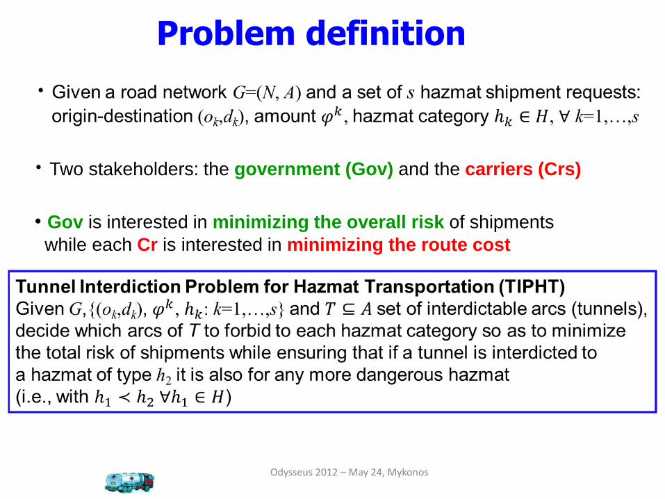
Problem definition

• Two stakeholders: the government (Gov) and the carriers (Crs)

• Gov is interested in minimizing the overall risk of shipments

while each Cr is interested in minimizing the route cost


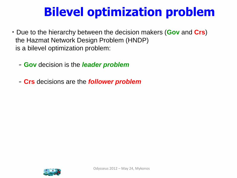
Bilevel optimization problem

- Gov decision is the leader problem

• Due to the hierarchy between the decision makers (Gov and Crs)

the Hazmat Network Design Problem (HNDP)

is a bilevel optimization problem:

- Crs decisions are the follower problem

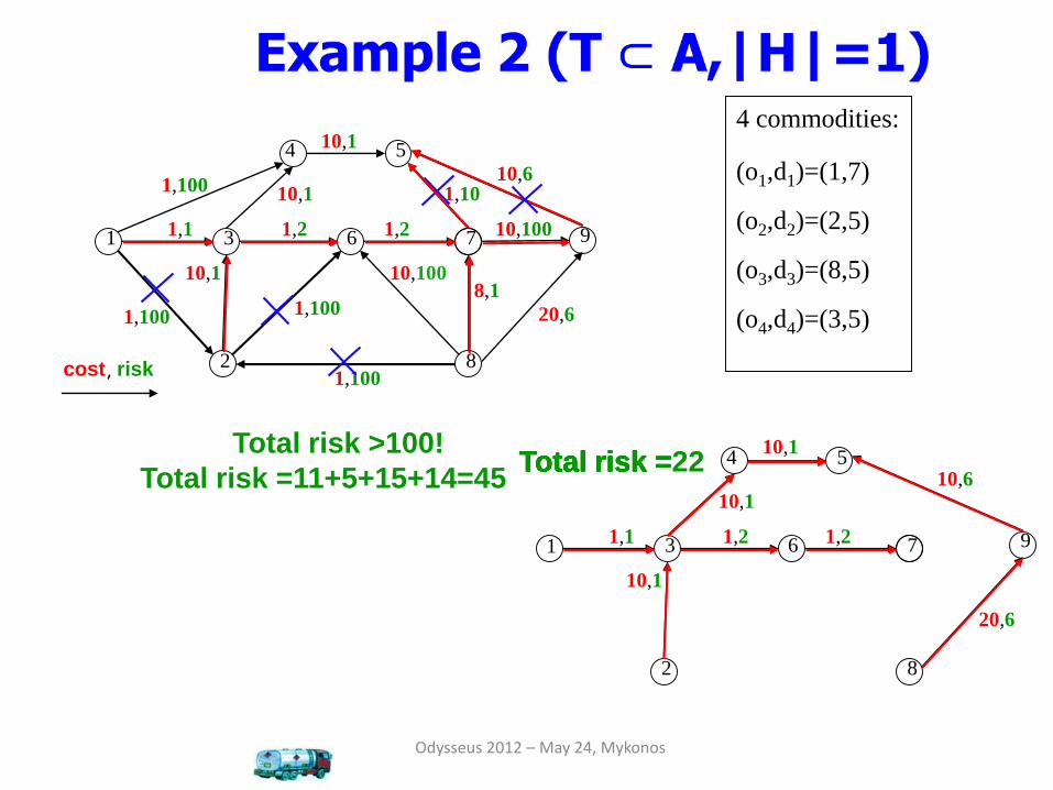
cost, risk

4 commodities:

(o1,d1)=(1,7)

(o2,d2)=(2,5)

(o3,d3)=(8,5)

(o4,d4)=(3,5)

1

2 8

54

3 6 7

1,100

1,1

1,100

1,100

10,100

1,100

10,1

1,2 1,2

8,1

10,100

1,1010,1

10,1

9

10,6

20,6

1

2 8

54

3 6 71,1

10,1

1,2 1,2

8,1

1,1010,1

10,1Total risk =

5

Total risk =

5+15

Total risk =

5+15+11

Total risk =

5+15+11+14

Total risk = 45

1

2 8

54

3 6 71,1

10,1

1,2 1,2

10,1

10,1

9

10,6

20,6

Total risk =

5

Total risk =

5+3

Total risk =

5+3+12

Total risk =

5+3+12+2

Total risk =22

Example 1 (T=A,|H|=1)



cost, risk

4 commodities:

(o1,d1)=(1,7)

(o2,d2)=(2,5)

(o3,d3)=(8,5)

(o4,d4)=(3,5)

1

2 8

54

3 6 7

1,100

1,1

1,100

1,100

10,100

1,100

10,1

1,2 1,2

8,1

10,100

1,1010,1

10,1

9

10,6

20,6

1

2 8

54

3 6 71,1

10,1

1,2 1,2

10,1

10,1

9

10,6

20,6

Total risk =Total risk =Total risk Total risk =Total risk =22Total risk >100!

Total risk =11+5+15+14=45


Literature

• Kara, Verter “Designing a road network for hazardous materials transportation”, Transp.Science 04:

first bilevel formulation (just with T = A) and a single level one obtainend linearizing the KKT conditions of the follower

• Erkut, Alp “Designing a road network for dangerous goods shipments”,

C.O.R. 09:

restrict the network to a tree

• Erkut, Gzara “Solving the hazmat transport network design problem”,

C.O.R. 08:

heuristics to find stable solutions (that consider the worst case risk when

the follower has multiple optimal solutions)


Literature

• E.Amaldi, M.Bruglieri, B.Fortz, On the hazmat transport network design problem, INOC ’11:

- HNDP extension where a subset T of roads can be interdicted- proof of NP-hardness even for a single o-d pair- bilevel MILP formulation that guarantees stability- single-level MILP reformulation that can be solved more efficientlythan Kara-Verter’s one (|T | binary variables rather than s|A|+|T |)


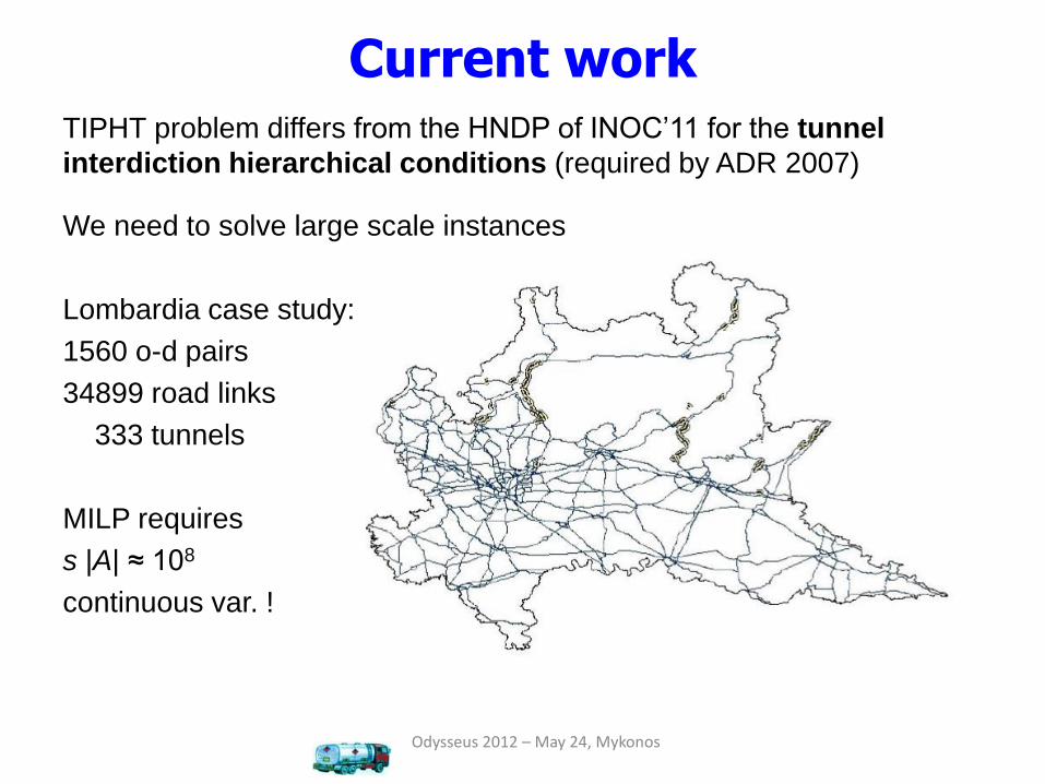
Current workTIPHT problem differs from the HNDP of INOC’11 for the tunnel

interdiction hierarchical conditions (required by ADR 2007)

We need to solve large scale instances

Lombardia case study:

1560 o-d pairs

34899 road links

333 tunnels

MILP requires

s |A| ≈ 108

continuous var. !


Instance of Lombardia

Lombardia region: a large and interesting case (many tunnels and o-d pairs)

P.Gandini, MS Thesis (in Italian), PoliMI, 2009

• o-d pairs: 40x40 (partitioning each province in subareas)

• Hazmat shipment estimation:

Conto Nazionale Trasporto

(ISTAT 2004)

+ Gross Domestic Product

• Risk assessment in tunnels

and in the open-topped

roads for each hazmat category

(population exposed,

environment,…)


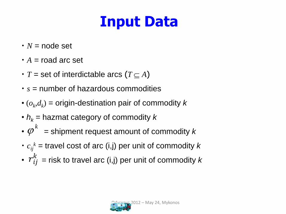
Input Data

• N = node set

• A = road arc set

• T = set of interdictable arcs (T A)

• s = number of hazardous commodities

• (ok,dk) = origin-destination pair of commodity k

• hk = hazmat category of commodity k

• = shipment request amount of commodity k

• cijk = travel cost of arc (i,j) per unit of commodity k

• = risk to travel arc (i,j) per unit of commodity k

k


Decision variables

Gov variables

HhTjih

ji

yh

ij

= ,),(

otherwise0

category hazmat to

allowed is),( arc if1

Crs variables

skAji ,...,1,),( =

=otherwise0

shipment for chosen is )( arc if1 ki,jx

k

ij


Bilevel ILP formulation

where variables are solution of:k

ijx

skNj

dj

oj

doj

xx

k

k

kk

jl

k

jl

ji

k

ij ,...,1,,

if1

if1-

,if0

)()(

=

=

=

=− +−

(5)

skTjiyx kh

ij

k

ij ,...,1,),( = (6)

=

s

Aji

k

ij

kh

ijk

k xr1 ),(

min (1)

(7),...,1,),( skAji =

=

s

Aji

k

ij

k

ijk

xc1 ),(

min (4)

2121 :,,),(21 hhHhhTjiyyh

ij

h

ij (2)

HhTjiyh

ij ,),(},1,0{ (3)


Solving bilevel formulation

Applying strong LP duality, we substitute the inner problem with constraints:

(9) ,...,1,\),( skTAjicwwk

ij

k

i

k

j =−

(10) ,...,1,),( )1( skTjiyMcww kh

ij

k

ij

k

i

k

j =−+−

Dual

feasibility

(11) ,...,1 ),(

skwwxck

o

k

d

Aji

k

ij

k

ij kk=−=

primal o.f. = dual o.f.

skTjiyx kh

ij

k

ij ,...,1,),( = (6)

skNj

dj

oj

doj

xx

k

k

kk

jl

k

jl

ji

k

ij ,...,1,,

if1

if1-

,if0

)()(

=

=

=

=− +−

(5)

Primal

feasibility

(8)skAjixk

ij ,...,1,),(0 =


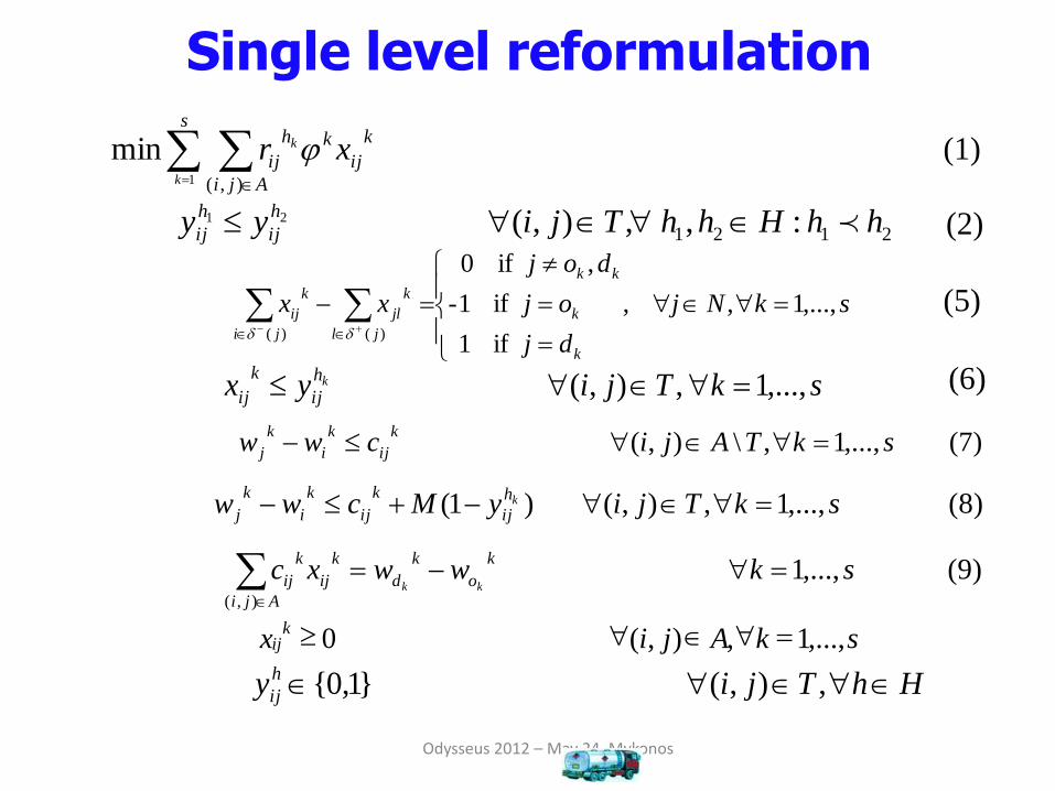
Single level reformulation

(7) ,...,1,\),( skTAjicwwk

ij

k

i

k

j =−

(8) ,...,1,),( )1( skTjiyMcww kh

ij

k

ij

k

i

k

j =−+−

(9) ,...,1 ),(

skwwxck

o

k

d

Aji

k

ij

k

ij kk=−=

skTjiyx kh

ij

k

ij ,...,1,),( = (6)

skNj

dj

oj

doj

xx

k

k

kk

jl

k

jl

ji

k

ij ,...,1,,

if1

if1-

,if0

)()(

=

=

=

=− +−

(5)

skAjixk

ij ,...,1,),(0 =

=

s

Aji

k

ij

kh

ijk

k xr1 ),(

min (1)

HhTjiyh

ij ,),(}1,0{


ij

h

ij (2)


Lagrangean relaxation

(7) ,...,1,\),( skTAjicwwk

ij

k

i

k

j =−

(8) ,...,1,),( )1( skTjiyMcww kh

ij

k

ij

k

i

k

j =−+−

(9) ,...,1 ),(

skwwxck

o

k

d

Aji

k

ij

k

ij kk=−=

skTjiyx kh

ij

k

ij ,...,1,),( = (6)

skNj

dj

oj

doj

xx

k

k

kk

jl

k

jl

ji

k

ij ,...,1,,

if1

if1-

,if0

)()(

=

=

=

=− +−

(5)

skAjixk

ij ,...,1,),(0 =

=

s

Aji

k

ij

kh

ijk

k xr1 ),(

min

HhTjiyh

ij ,),(}1,0{


ij

h

ij (2)

)(1 ),(

k

k

h

ij

s

Tji

k

ij

k

ij yx =

−+ ][....1 ),(

=

+s

Tji

k

ijk

=),( L


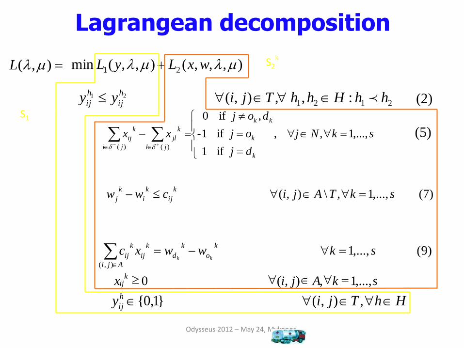
Lagrangean decomposition

(7) ,...,1,\),( skTAjicwwk

ij

k

i

k

j =−

(9) ,...,1 ),(

skwwxck

o

k

d

Aji

k

ij

k

ij kk=−=

skNj

dj

oj

doj

xx

k

k

kk

jl

k

jl

ji

k

ij ,...,1,,

if1

if1-

,if0

)()(

=

=

=

=− +−

(5)

skAjixk

ij ,...,1,),(0 =

),,,(),,(min 21 wxLyL +

HhTjiyh

ij ,),(}1,0{


ij

h

ij (2)

=),( L

S1

S2k


Lagrangean dual

We solve the Lagrangean dual via the subgradient method:

)(,0max),(

,0max kh

ij

k

ij

k

ijk

ij

k

ij

k

ij yxL

−+=

+=

2),(

)),(( where

L

LRUB

−=

+

+−+=

+=

Mc

MywwLk

ij

h

ij

k

i

k

jk

ijk

ij

k

ij

k

ij

k

,0max

),(,0max

iterations 30every halved and 2 == n


Lagrangean heuristic

(8) ,...,1,),( )1( skTjiyMcww kh

ij

k

ij

k

i

k

j =−+−

skTjiyx kh

ij

k

ij ,...,1,),( = (6)

Relaxed solution may generate paths passing through tunnels closed

Relaxed solution may generate paths with non minimum cost

1. we consider closed each tunnel (i,j) s.t.

in the solution of S1

2. For each commodity k we solve a minimum path problem

on a graph where all tunnels closed for category hk are eliminated

0=h

ijyHh

Some computational results

• Lecco instance:

12 o-d pairs (12∙3=36 shipment requests)

R* Rheur L (Rheur -R*)/R* (R* -L)/R*

98907 102049 93869 3.18% 5.40%

22 iterations of subgradient method (CPU time limit=24h)

• PC Intel Xeon 2.80 GHz and 512KB L2 cache, 2GB RAM

• For practical reasons S2k

and Lagrangean heuristic min path problems

are solved by AMPL-CPLEX 11.0


Risk reduction of 16.3% compared to the unregulated scenario

Some computational results

• Brescia instance:

32 o-d pairs (32∙3=96 shipment requests)

-200000

0

200000

400000

600000

800000

1000000

1200000

1 2 3 4 5 6 7 8 9 10

Upper Bound

value L


Rheur L (Rheur -L)/L

493880 451926 8.49%

Risk reduction of 52.3% compared to the deregulated scenario!

(CPU time limit=24h)

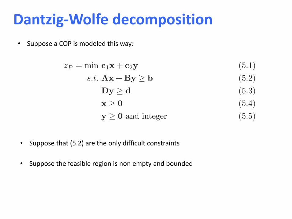
Dantzig-Wolfe decomposition

• Suppose a COP is modeled this way:

• Suppose that (5.2) are the only difficult constraints

• Suppose the feasible region is non empty and bounded

Dantzig-Wolfe decomposition

• Let 𝐹 = 𝑥, 𝑦 : 𝐷𝑦 ≥ 𝑑, 𝑥 ≥ 0, 𝑦 ≥ 0 and integer which we assume bounded and non empty

• Let { 𝑥𝑡, 𝑦𝑡 : 𝑡 = 1,… , 𝑇} be the extreme points of F

• Main idea: ➢ With a subproblem we identify the extreme points of F that are optimal w.r.t. the

current objective function➢ With the master problem we compute the best convex combination of the

current extreme points that also satisfy the relaxed constraints (5.2)

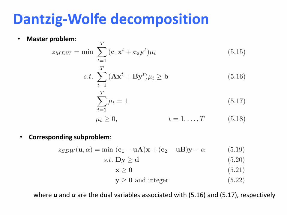
Dantzig-Wolfe decomposition• Master problem:

• Corresponding subproblem:

where u and α are the dual variables associated with (5.16) and (5.17), respectively

Dantzig-Wolfe decomposition matheur.

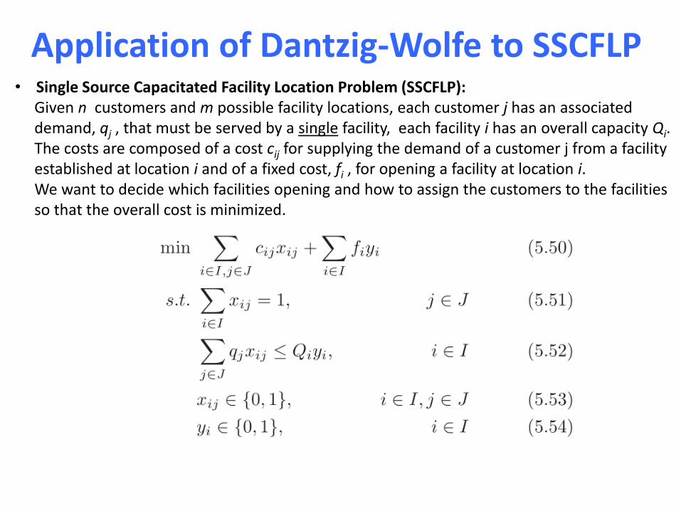
Application of Dantzig-Wolfe to SSCFLP• Single Source Capacitated Facility Location Problem (SSCFLP):

Given n customers and m possible facility locations, each customer j has an associated demand, qj , that must be served by a single facility, each facility i has an overall capacity Qi. The costs are composed of a cost cij for supplying the demand of a customer j from a facility established at location i and of a fixed cost, fi , for opening a facility at location i. We want to decide which facilities opening and how to assign the customers to the facilities so that the overall cost is minimized.

Application of Dantzig-Wolfe to SSCFLP• Master problem:

• Corresponding subproblem:

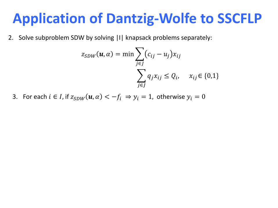
Application of Dantzig-Wolfe to SSCFLP2. Solve subproblem SDW by solving |I| knapsack problems separately:

𝑧𝑆𝐷𝑊 𝒖, 𝛼 = min

𝑗∈𝐽

𝑐𝑖𝑗 − 𝑢𝑗 𝑥𝑖𝑗

𝑗∈𝐽

𝑞𝑗𝑥𝑖𝑗 ≤ 𝑄𝑖 , 𝑥𝑖𝑗∈ {0,1}

3. For each 𝑖 ∈ 𝐼, if 𝑧𝑆𝐷𝑊 𝒖, 𝛼 < −𝑓𝑖 ⇒ 𝑦𝑖 = 1, otherwise 𝑦𝑖 = 0

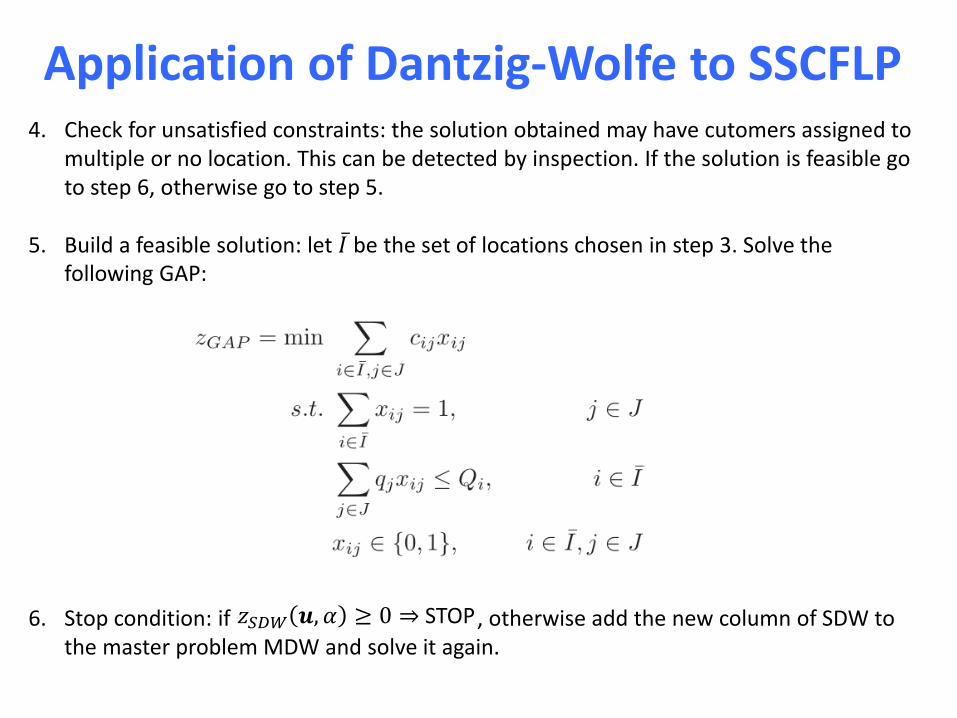
4. Check for unsatisfied constraints: the solution obtained may have cutomers assigned to multiple or no location. This can be detected by inspection. If the solution is feasible go to step 6, otherwise go to step 5.

5. Build a feasible solution: let ҧ𝐼 be the set of locations chosen in step 3. Solve the following GAP:

6. Stop condition: if , otherwise add the new column of SDW to the master problem MDW and solve it again.

Application of Dantzig-Wolfe to SSCFLP

𝑧𝑆𝐷𝑊 𝒖, 𝛼 ≥ 0 ⇒ STOP

References• M. O. Ball, (2011). Heuristics based on mathematical programming. Surveys in

Operations Research and Management Science, 16, pp. 21-38.

• M. Boschetti, V.Maniezzo, M. Roffilli, (2009). Decomposition techniques as metaheuristic frameworks. In: V. Maniezzo et al, (eds), Matheuristics, Annals of Information Systems, 10, pp. 135-157

• M. Boschetti and V. Maniezzo, (2009). Benders decomposition, Lagrangeanrelaxation and metaheuristic design. Journal of Heuristics, 15(3):283–312.

• J. Cordeau, G. Stojkociv, F. Soumis, J. Desrosiers, (2001). Benders decomposition for simultaneous aircraft routing and crew scheduling, Transportation Science 35.

• M. Fisher, R. Jaikumar, (1981). A generalized assignment heuristic for the vehiclerouting problem, Networks 11, 109–124

• M. Guignard, S. Kim, (1987). Lagrangean decomposition: A model yielding stronger lagrangean bounds, Mathematical Programming 39, 215-228.

matheuristics for combinatorial optimization problems

Documents