matlab fundamentals - metucourses.me.metu.edu.tr/courses/me582/files/matlab tutorial - chapra.pdf32...
TRANSCRIPT

CHAPTER OBJECTIVES
Knowledge and understanding are prerequisites for the effective implementation of any tool.
No matter how impressive your tool chest, you will be hard-pressed to repair a car if you do not understand how it works.
• This is the first chapter objectives entry.• Second chapter objective entry, the entries use ic/lc per manuscript, the first and
last entry have space above or below, middle entries do not.• Third chapter entry copy goes here.
MATLAB Fundamentals
27
2MATLAB Fundamentals
CHAPTER OBJECTIVES
The primary objective of this chapter is to provide an introduction and overview of how MATLAB’s calculator mode is used to implement interactive computations. Specific objectives and topics covered are
• Learning how real and complex numbers are assigned to variables.• Learning how vectors and matrices are assigned values using simple assignment,
the colon operator, and the linspace and logspace functions.• Understanding the priority rules for constructing mathematical expressions.• Gaining a general understanding of built-in functions and how you can learn more
about them with MATLAB’s Help facilities.• Learning how to use vectors to create a simple line plot based on an equation.
YOU’VE GOT A PROBLEM
In Chap. 1, we used a force balance to determine the terminal velocity of a free-falling object like a bungee jumper:
υt = √___
gm ___ cd
where υt = terminal velocity (m/s), g = gravitational acceleration (m/s2), m = mass (kg), and cd = a drag coefficient (kg/m). Aside from predicting the terminal velocity, this equa-tion can also be rearranged to compute the drag coefficient
cd = mg ___ υ t 2
(2.1)
cha97962_ch02_027-052.indd 27 08/11/16 3:21 pm

28 MATLAB FundAMenTALs
Thus, if we measure the terminal velocity of a number of jumpers of known mass, this equation provides a means to estimate the drag coefficient. The data in Table 2.1 were col-lected for this purpose.
In this chapter, we will learn how MATLAB can be used to analyze such data. Beyond showing how MATLAB can be employed to compute quantities like drag coefficients, we will also illustrate how its graphical capabilities provide additional insight into such analyses.
2.1 THE MATLAB ENVIRONMENT
MATLAB is a computer program that provides the user with a convenient environment for performing many types of calculations. In particular, it provides a very nice tool to imple-ment numerical methods.
The most common way to operate MATLAB is by entering commands one at a time in the command window. In this chapter, we use this interactive or calculator mode to in-troduce you to common operations such as performing calculations and creating plots. In Chap. 3, we show how such commands can be used to create MATLAB programs.
One further note. This chapter has been written as a hands-on exercise. That is, you should read it while sitting in front of your computer. The most efficient way to become proficient is to actually implement the commands on MATLAB as you proceed through the following material.
MATLAB uses three primary windows:• Command window. Used to enter commands and data.• Graphics window. Used to display plots and graphs.• Edit window. Used to create and edit M-files.
In this chapter, we will make use of the command and graphics windows. In Chap. 3 we will use the edit window to create M-files.
After starting MATLAB, the command window will open with the command prompt being displayed
>>
The calculator mode of MATLAB operates in a sequential fashion as you type in com-mands line by line. For each command, you get a result. Thus, you can think of it as operat-ing like a very fancy calculator. For example, if you type in
>> 55 − 16
MATLAB will display the result1
ans = 39
TABLE 2.1 data for the mass and associated terminal velocities of a number of jumpers.
m, kg 83.6 60.2 72.1 91.1 92.9 65.3 80.9υt , m/s 53.4 48.5 50.9 55.7 54 47.7 51.1
1 MATLAB skips a line between the label (ans =) and the number (39). Here, we omit such blank lines for conciseness. You can control whether blank lines are included with the format compact and format loose commands.
cha97962_ch02_027-052.indd 28 08/11/16 3:21 pm

2.2 AssIGnMenT 29
Notice that MATLAB has automatically assigned the answer to a variable, ans. Thus, you could now use ans in a subsequent calculation:
>> ans + 11
with the result
ans = 50
MATLAB assigns the result to ans whenever you do not explicitly assign the calculation to a variable of your own choosing.
2.2 ASSIGNMENT
Assignment refers to assigning values to variable names. This results in the storage of the values in the memory location corresponding to the variable name.
2.2.1 Scalars
The assignment of values to scalar variables is similar to other computer languages. Try typing
>> a = 4
Note how the assignment echo prints to confirm what you have done:
a = 4
Echo printing is a characteristic of MATLAB. It can be suppressed by terminating the com-mand line with the semicolon (;) character. Try typing
>> A = 6;
You can type several commands on the same line by separating them with commas or semicolons. If you separate them with commas, they will be displayed, and if you use the semicolon, they will not. For example,
>> a = 4,A = 6;x = 1;
a = 4
MATLAB treats names in a case-sensitive manner—that is, the variable a is not the same as A. To illustrate this, enter
>> a
and then enter
>> A
See how their values are distinct. They are distinct names.
cha97962_ch02_027-052.indd 29 08/11/16 3:21 pm

30 MATLAB FundAMenTALs
We can assign complex values to variables, since MATLAB handles complex arith-metic automatically. The unit imaginary number √
___ −1 is preassigned to the variable i.
Consequently, a complex value can be assigned simply as in
>> x = 2 +i*4
x = 2.0000 + 4.0000i
It should be noted that MATLAB allows the symbol j to be used to represent the unit imaginary number for input. However, it always uses an i for display. For example,
>> x = 2 +j*4
x = 2.0000 + 4.0000i
There are several predefined variables, for example, pi.
>> pi
ans = 3.1416
Notice how MATLAB displays four decimal places. If you desire additional precision, enter the following:
>> format long
Now when pi is entered the result is displayed to 15 significant figures:
>> pi
ans = 3.14159265358979
To return to the four decimal version, type
>> format short
The following is a summary of the format commands you will employ routinely in engi-neering and scientific calculations. They all have the syntax: format type.
type Result Example
short Scaled fixed-point format with 5 digits 3.1416long Scaled fixed-point format with 15 digits for double and 7 digits for single 3.14159265358979short e Floating-point format with 5 digits 3.1416e+000long e Floating-point format with 15 digits for double and 7 digits for single 3.141592653589793e+000short g Best of fixed- or floating-point format with 5 digits 3.1416long g Best of fixed- or floating-point format with 15 digits for double 3.14159265358979 and 7 digits for singleshort eng Engineering format with at least 5 digits and a power that is a multiple of 3 3.1416e+000long eng Engineering format with exactly 16 significant digits and a power 3.14159265358979e+000 that is a multiple of 3bank Fixed dollars and cents 3.14
cha97962_ch02_027-052.indd 30 08/11/16 3:21 pm

2.2 AssIGnMenT 31
2.2.2 Arrays, Vectors, and Matrices
An array is a collection of values that are represented by a single variable name. One- dimensional arrays are called vectors and two-dimensional arrays are called matrices. The scalars used in Sec. 2.2.1 are actually matrices with one row and one column.
Brackets are used to enter arrays in the command mode. For example, a row vector can be assigned as follows:
>> a = [1 2 3 4 5]
a = 1 2 3 4 5
Note that this assignment overrides the previous assignment of a = 4.In practice, row vectors are rarely used to solve mathematical problems. When we
speak of vectors, we usually refer to column vectors, which are more commonly used. A column vector can be entered in several ways. Try them.
>> b = [2;4;6;8;10]
or>> b = [246810]
or, by transposing a row vector with the ' operator,>> b = [2 4 6 8 10]'
The result in all three cases will beb = 2 4 6 8 10
A matrix of values can be assigned as follows:
>> A = [1 2 3; 4 5 6; 7 8 9]
A = 1 2 3 4 5 6 7 8 9
In addition, the Enter key (carriage return) can be used to separate the rows. For example, in the following case, the Enter key would be struck after the 3, the 6, and the ] to assign the matrix:
>> A = [1 2 3 4 5 6 7 8 9]
cha97962_ch02_027-052.indd 31 08/11/16 3:21 pm

32 MATLAB FundAMenTALs
Finally, we could construct the same matrix by concatenating (i.e., joining) the vectors representing each column:
>> A = [[1 4 7]' [2 5 8]' [3 6 9]']
At any point in a session, a list of all current variables can be obtained by entering the who command:
>> who
Your variables are:A a ans b x
or, with more detail, enter the whos command:>> whos
Name Size Bytes Class
A 3x3 72 double array a 1x5 40 double array ans 1x1 8 double array b 5x1 40 double array x 1x1 16 double array (complex)
Grand total is 21 elements using 176 bytes
Note that subscript notation can be used to access an individual element of an array. For example, the fourth element of the column vector b can be displayed as
>> b(4)
ans = 8
For an array, A(m,n) selects the element in mth row and the nth column. For example,>> A(2,3)
ans = 6
There are several built-in functions that can be used to create matrices. For exam-ple, the ones and zeros functions create vectors or matrices filled with ones and zeros, respectively. Both have two arguments, the first for the number of rows and the second for the number of columns. For example, to create a 2 × 3 matrix of zeros:
>> E = zeros(2,3)
E = 0 0 0 0 0 0
Similarly, the ones function can be used to create a row vector of ones:>> u = ones(1,3)
u = 1 1 1
cha97962_ch02_027-052.indd 32 08/11/16 3:21 pm
2.2 AssIGnMenT 33
2.2.3 The Colon Operator
The colon operator is a powerful tool for creating and manipulating arrays. If a colon is used to separate two numbers, MATLAB generates the numbers between them using an increment of one:
>> t = 1:5
t = 1 2 3 4 5
If colons are used to separate three numbers, MATLAB generates the numbers between the first and third numbers using an increment equal to the second number:
>> t = 1:0.5:3
t = 1.0000 1.5000 2.0000 2.5000 3.0000
Note that negative increments can also be used
>> t = 10:−1:5
t = 10 9 8 7 6 5
Aside from creating series of numbers, the colon can also be used as a wildcard to select the individual rows and columns of a matrix. When a colon is used in place of a specific subscript, the colon represents the entire row or column. For example, the second row of the matrix A can be selected as in
>> A(2,:)
ans = 4 5 6
We can also use the colon notation to selectively extract a series of elements from within an array. For example, based on the previous definition of the vector t:
>> t(2:4)
ans = 9 8 7
Thus, the second through the fourth elements are returned.
2.2.4 The linspace and logspace Functions
The linspace and logspace functions provide other handy tools to generate vectors of spaced points. The linspace function generates a row vector of equally spaced points. It has the form
linspace(x1, x2, n)
cha97962_ch02_027-052.indd 33 08/11/16 3:21 pm
34 MATLAB FundAMenTALs
which generates n points between x1 and x2. For example>> linspace(0,1,6)
ans = 0 0.2000 0.4000 0.6000 0.8000 1.0000
If the n is omitted, the function automatically generates 100 points.The logspace function generates a row vector that is logarithmically equally spaced. It
has the form
logspace(x1, x2, n)
which generates n logarithmically equally spaced points between decades 10x1 and 10x2. For example,
>> logspace(-1,2,4)
ans = 0.1000 1.0000 10.0000 100.0000
If n is omitted, it automatically generates 50 points.
2.2.5 Character Strings
Aside from numbers, alphanumeric information or character strings can be represented by enclosing the strings within single quotation marks. For example,
>> f = 'Miles ';>> s = 'Davis';
Each character in a string is one element in an array. Thus, we can concatenate (i.e., paste together) strings as in
>> x = [f s]
x =Miles Davis
Note that very long lines can be continued by placing an ellipsis (three consecutive periods) at the end of the line to be continued. For example, a row vector could be entered as
>> a = [1 2 3 4 5 ...6 7 8]
a = 1 2 3 4 5 6 7 8
However, you cannot use an ellipsis within single quotes to continue a string. To enter a string that extends beyond a single line, piece together shorter strings as in
>> quote = ['Any fool can make a rule,' ...' and any fool will mind it']
quote =Any fool can make a rule, and any fool will mind it
cha97962_ch02_027-052.indd 34 08/11/16 3:21 pm

2.2 AssIGnMenT 35
TABLE 2.2 some useful string functions.
Function Description
n=length(s) Number of characters, n, in a string, s.
b=strcmp(s1,s2) Compares two strings, s1 and s2; if equal returns true (b = 1). If not equal, returns false (b = 0).
n=str2num(s) Converts a string, s, to a number, n.
s=num2str(n) Converts a number, n, to a string, s.
s2=strrep(s1,c1,c2) Replaces characters in a string with different characters.
i=strfind(s1,s2) Returns the starting indices of any occurrences of the string s2 in the string s1.
S=upper(s) Converts a string to upper case.
s=lower(S) Converts a string to lower case.
A number of built-in MATLAB functions are available to operate on strings. Table 2.2 lists a few of the more commonly used ones. For example,
>> x1 = ‘Canada’; x2 = ‘Mexico’; x3 = ‘USA’; x4 = ‘2010’; x5 = 810;
>> strcmp(a1,a2)
ans =
0
>> strcmp(x2,’Mexico’)
ans =
1
>> str2num(x4)
ans =
2010
>> num2str(x5)
ans =
810
>> strrep
>> lower
>> upper
Note, if you want to display strings in multiple lines, use the sprint function and insert the two-character sequence \n between the strings. For example,
>> disp(sprintf('Yo\nAdrian!'))
yields
Yo
Adrian!
cha97962_ch02_027-052.indd 35 08/11/16 3:21 pm

36 MATLAB FundAMenTALs
2.3 MATHEMATICAL OPERATIONS
Operations with scalar quantities are handled in a straightforward manner, similar to other computer languages. The common operators, in order of priority, are
^ Exponentiation− Negation* / Multiplication and division\ Left division2
+ − Addition and subtraction
These operators will work in calculator fashion. Try
>> 2*pi
ans = 6.2832
Also, scalar real variables can be included:
>> y = pi/4;>> y ^ 2.45
ans = 0.5533
Results of calculations can be assigned to a variable, as in the next-to-last example, or simply displayed, as in the last example.
As with other computer calculation, the priority order can be overridden with paren-theses. For example, because exponentiation has higher priority than negation, the follow-ing result would be obtained:
>> y = −4 ^ 2
y = −16
Thus, 4 is first squared and then negated. Parentheses can be used to override the priorities as in
>> y = (−4) ^ 2
y = 16
Within each precedence level, operators have equal precedence and are evaluated from left to right. As an example,
>> 4^2^3>> 4^(2^3)>> (4^2)^3
2 Left division applies to matrix algebra. It will be discussed in detail later in this book.
cha97962_ch02_027-052.indd 36 08/11/16 3:21 pm

2.3 MATheMATIcAL OperATIOns 37
In the first case 42 = 16 is evaluated first, which is then cubed to give 4096. In the second case 23 = 8 is evaluated first and then 48 = 65,536. The third case is the same as the first, but uses parentheses to be clearer.
One potentially confusing operation is negation; that is, when a minus sign is em-ployed with a single argument to indicate a sign change. For example,
>> 2*−4
The −4 is treated as a number, so you get −8. As this might be unclear, you can use paren-theses to clarify the operation
>> 2*(−4)
Here is a final example where the minus is used for negation
>> 2^−4
Again −4 is treated as a number, so 2^−4 = 2−4 = 1/24 = 1/16 = 0.0625. Parentheses can make the operation clearer
>> 2^(−4)
Calculations can also involve complex quantities. Here are some examples that use the values of x (2 + 4i) and y (16) defined previously:
>> 3 * x
ans = 6.0000 + 12.0000i
>> 1 / x
ans = 0.1000 − 0.2000i
>> x ^ 2
ans = −12.0000 + 16.0000i
>> x + y
ans = 18.0000 + 4.0000i
The real power of MATLAB is illustrated in its ability to carry out vector-matrix calculations. Although we will describe such calculations in detail in Chap. 8, it is worth introducing some examples here.
The inner product of two vectors (dot product) can be calculated using the * operator,
>> a * b
ans = 110
cha97962_ch02_027-052.indd 37 08/11/16 3:21 pm

38 MATLAB FundAMenTALs
and likewise, the outer product
>> b * a
ans = 2 4 6 8 10 4 8 12 16 20 6 12 18 24 30 8 16 24 32 40 10 20 30 40 50
To further illustrate vector-matrix multiplication, first redefine a and b:>> a = [1 2 3];
and>> b = [4 5 6]';
Now, try>> a * A
ans = 30 36 42
or>> A * b
ans = 32 77 122
Matrices cannot be multiplied if the inner dimensions are unequal. Here is what happens when the dimensions are not those required by the operations. Try
>> A * a
MATLAB automatically displays the error message:
??? Error using ==> mtimesInner matrix dimensions must agree.
Matrix-matrix multiplication is carried out in likewise fashion:
>> A * A
ans = 30 36 42 66 81 96 102 126 150
Mixed operations with scalars are also possible:
>> A/pi
ans = 0.3183 0.6366 0.9549 1.2732 1.5915 1.9099 2.2282 2.5465 2.8648
cha97962_ch02_027-052.indd 38 08/11/16 3:21 pm

2.4 use OF BuILT-In FuncTIOns 39
We must always remember that MATLAB will apply the simple arithmetic operators in vector-matrix fashion if possible. At times, you will want to carry out calculations item by item in a matrix or vector. MATLAB provides for that too. For example,
>> A^2
ans = 30 36 42 66 81 96 102 126 150
results in matrix multiplication of A with itself.What if you want to square each element of A? That can be done with>> A.^2
ans = 1 4 9 16 25 36 49 64 81
The . preceding the ^ operator signifies that the operation is to be carried out element by element. The MATLAB manual calls these array operations. They are also often referred to as element-by-element operations.
MATLAB contains a helpful shortcut for performing calculations that you’ve already done. Press the up-arrow key. You should get back the last line you typed in.
>> A.^2
Pressing Enter will perform the calculation again. But you can also edit this line. For example, change it to the line below and then press Enter.
>> A.^3
ans = 1 8 27 64 125 216 343 512 729
Using the up-arrow key, you can go back to any command that you entered. Press the up-arrow until you get back the line
>> b * a
Alternatively, you can type b and press the up-arrow once and it will automatically bring up the last command beginning with the letter b. The up-arrow shortcut is a quick way to fix errors without having to retype the entire line.
2.4 USE OF BUILT-IN FUNCTIONS
MATLAB and its Toolboxes have a rich collection of built-in functions. You can use online help to find out more about them. For example, if you want to learn about the log function, type in
>> help log
LOG Natural logarithm.
cha97962_ch02_027-052.indd 39 08/11/16 3:21 pm

40 MATLAB FundAMenTALs
LOG(X) is the natural logarithm of the elements of X. Complex results are produced if X is not positive.
See also LOG2, LOG10, EXP, LOGM.
For a list of all the elementary functions, type>> help elfun
One of their important properties of MATLAB’s built-in functions is that they will operate directly on vector and matrix quantities. For example, try
>> log(A)
ans = 0 0.6931 1.0986 1.3863 1.6094 1.7918 1.9459 2.0794 2.1972
and you will see that the natural logarithm function is applied in array style, element by element, to the matrix A. Most functions, such as sqrt, abs, sin, acos, tanh, and exp, operate in array fashion. Certain functions, such as exponential and square root, have matrix defini-tions also. MATLAB will evaluate the matrix version when the letter m is appended to the function name. Try
>> sqrtm(A)
ans = 0.4498 + 0.7623i 0.5526 + 0.2068i 0.6555 − 0.3487i 1.0185 + 0.0842i 1.2515 + 0.0228i 1.4844 − 0.0385i 1.5873 − 0.5940i 1.9503 − 0.1611i 2.3134 + 0.2717i
There are several functions for rounding. For example, suppose that we enter a vector:>> E = [−1.6 −1.5 −1.4 1.4 1.5 1.6];
The round function rounds the elements of E to the nearest integers:>> round(E)
ans = −2 −2 −1 1 2 2
The ceil (short for ceiling) function rounds to the nearest integers toward infinity:>> ceil(E)
ans = −1 −1 −1 2 2 2
The floor function rounds down to the nearest integers toward minus infinity:>> floor(E)
ans = −2 −2 −2 1 1 1
There are also functions that perform special actions on the elements of matrices and arrays. For example, the sum function returns the sum of the elements:
>> F = [3 5 4 6 1];>> sum(F)
ans = 19
cha97962_ch02_027-052.indd 40 08/11/16 3:21 pm

2.4 use OF BuILT-In FuncTIOns 41
In a similar way, it should be pretty obvious what’s happening with the following commands:
>> min(F),max(F),mean(F),prod(F),sort(F)
ans = 1
ans = 6
ans = 3.8000
ans = 360
ans = 1 3 4 5 6
A common use of functions is to evaluate a formula for a series of arguments. Recall that the velocity of a free-falling bungee jumper can be computed with [Eq. (1.9)]:
υ = √___
gm ___ cd tanh ( √____
gcd ____ m t )
where υ is velocity (m/s), g is the acceleration due to gravity (9.81 m/s2), m is mass (kg), cd is the drag coefficient (kg/m), and t is time (s).
Create a column vector t that contains values from 0 to 20 in steps of 2:>> t = [0:2:20]'
t = 0 2 4 6 8 10 12 14 16 18 20
Check the number of items in the t array with the length function:>> length(t)
ans = 11
Assign values to the parameters:>> g = 9.81; m = 68.1; cd = 0.25;
MATLAB allows you to evaluate a formula such as υ = f (t), where the formula is com-puted for each value of the t array, and the result is assigned to a corresponding position in the υ array. For our case,
cha97962_ch02_027-052.indd 41 08/11/16 3:21 pm
42 MATLAB FundAMenTALs
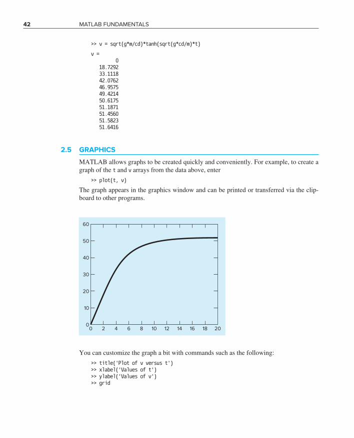
>> v = sqrt(g*m/cd)*tanh(sqrt(g*cd/m)*t)
v = 0 18.7292 33.1118 42.0762 46.9575 49.4214 50.6175 51.1871 51.4560 51.5823 51.6416
2.5 GRAPHICS
MATLAB allows graphs to be created quickly and conveniently. For example, to create a graph of the t and v arrays from the data above, enter
>> plot(t, v)
The graph appears in the graphics window and can be printed or transferred via the clip-board to other programs.
60
50
40
30
20
10
00 2 4 6 8 10 12 16 1814 20
You can customize the graph a bit with commands such as the following:>> title('Plot of v versus t')>> xlabel('Values of t')>> ylabel('Values of v')>> grid
cha97962_ch02_027-052.indd 42 08/11/16 3:21 pm

2.5 GrAphIcs 43
The plot command displays a solid thin blue line by default. If you want to plot each point with a symbol, you can include a specifier enclosed in single quotes in the plot function. Table 2.3 lists the available specifiers. For example, if you want to use open circles enter
>> plot(t, v, 'o')
60
50
40
30
20
10
00 2 4 6 8 10
Values of t
Plot of υ versus t
Val
ues
of υ
16 181412 20
TABLE 2.3 specifiers for colors, symbols, and line types.
Colors Symbols Line Types
Blue b Point . Solid −Green g Circle o Dotted :Red r X-mark x Dashdot -.Cyan c Plus + Dashed -- Magenta m Star *Yellow y Square sBlack k Diamond dWhite w Triangle(down)
^
Triangle(up) ^ Triangle(left) < Triangle(right) > Pentagram p Hexagram h
cha97962_ch02_027-052.indd 43 08/11/16 3:21 pm
44 MATLAB FundAMenTALs
You can also combine several specifiers. For example, if you want to use square green markers connected by green dashed lines, you could enter
>> plot(t, v, 's−−g')
You can also control the line width as well as the marker’s size and its edge and face (i.e., interior) colors. For example, the following command uses a heavier (2-point), dashed, cyan line to connect larger (10-point) diamond-shaped markers with black edges and magenta faces:
>> plot(x,y,'−−dc','LineWidth', 2,... 'MarkerSize',10,... 'MarkerEdgeColor','k',... 'MarkerFaceColor','m')
Note that the default line width is 1 point. For the markers, the default size is 6 point with blue edge color and no face color.
MATLAB allows you to display more than one data set on the same plot. For example, an alternative way to connect each data marker with a straight line would be to type
>> plot(t, v, t, v, 'o')
It should be mentioned that, by default, previous plots are erased every time the plot command is implemented. The hold on command holds the current plot and all axis proper-ties so that additional graphing commands can be added to the existing plot. The hold off command returns to the default mode. For example, if we had typed the following com-mands, the final plot would only display symbols:
>> plot(t, v)>> plot(t, v, 'o')
In contrast, the following commands would result in both lines and symbols being displayed:>> plot(t, v)>> hold on>> plot(t, v, 'o')>> hold off
In addition to hold, another handy function is subplot, which allows you to split the graph window into subwindows or panes. It has the syntax
subplot(m, n, p)
This command breaks the graph window into an m-by-n matrix of small axes, and selects the p-th axes for the current plot.
We can demonstrate subplot by examining MATLAB’s capability to generate three- dimensional plots. The simplest manifestation of this capability is the plot3 command which has the syntax
plot3(x, y, z)
where x, y, and z are three vectors of the same length. The result is a line in three-dimen-sional space through the points whose coordinates are the elements of x, y, and z.
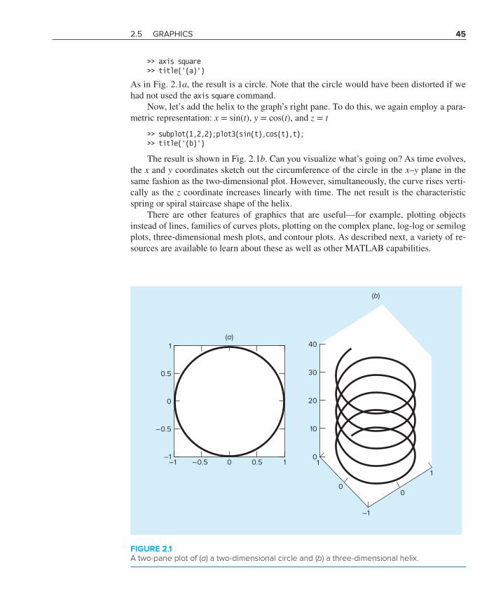
Plotting a helix provides a nice example to illustrate its utility. First, let’s graph a circle with the two-dimensional plot function using the parametric representation: x = sin(t) and y = cos(t). We employ the subplot command so we can subsequently add the three- dimensional plot.
>> t = 0:pi/50:10*pi;>> subplot(1,2,1);plot(sin(t),cos(t))
cha97962_ch02_027-052.indd 44 08/11/16 3:21 pm
2.5 GrAphIcs 45
>> axis square>> title('(a)')
As in Fig. 2.1a, the result is a circle. Note that the circle would have been distorted if we had not used the axis square command.
Now, let’s add the helix to the graph’s right pane. To do this, we again employ a para-metric representation: x = sin(t), y = cos(t), and z = t
>> subplot(1,2,2);plot3(sin(t),cos(t),t);>> title('(b)')
The result is shown in Fig. 2.1b. Can you visualize what’s going on? As time evolves, the x and y coordinates sketch out the circumference of the circle in the x–y plane in the same fashion as the two-dimensional plot. However, simultaneously, the curve rises verti-cally as the z coordinate increases linearly with time. The net result is the characteristic spring or spiral staircase shape of the helix.
There are other features of graphics that are useful—for example, plotting objects instead of lines, families of curves plots, plotting on the complex plane, log-log or semilog plots, three-dimensional mesh plots, and contour plots. As described next, a variety of re-sources are available to learn about these as well as other MATLAB capabilities.
40
30
20
10
01
0
−1
0
1
(a)
(b)
1
0.5
0
−0.5
−1−1 −0.5 0 0.5 1
FIGURE 2.1A two-pane plot of (a) a two-dimensional circle and (b) a three-dimensional helix.
cha97962_ch02_027-052.indd 45 08/11/16 3:21 pm

46 MATLAB FundAMenTALs
2.6 OTHER RESOURCES
The foregoing was designed to focus on those features of MATLAB that we will be using in the remainder of this book. As such, it is obviously not a comprehensive overview of all of MATLAB’s capabilities. If you are interested in learning more, you should consult one of the excellent books devoted to MATLAB (e.g., Attaway, 2009; Palm, 2007; Hanselman and Littlefield, 2005; and Moore, 2008).
Further, the package itself includes an extensive Help facility that can be accessed by clicking on the Help menu in the command window. This will provide you with a number of different options for exploring and searching through MATLAB’s Help material. In ad-dition, it provides access to a number of instructive demos.
As described in this chapter, help is also available in interactive mode by typing the help command followed by the name of a command or function.
If you do not know the name, you can use the lookfor command to search the MATLAB Help files for occurrences of text. For example, suppose that you want to find all the com-mands and functions that relate to logarithms, you could enter
>> lookfor logarithm
and MATLAB will display all references that include the word logarithm.Finally, you can obtain help from The MathWorks, Inc., website at www.mathworks
.com. There you will find links to product information, newsgroups, books, and technical support as well as a variety of other useful resources.
2.7 CASE STUDY eXpLOrATOrY dATA AnALYsIs
Background. Your textbooks are filled with formulas developed in the past by re-nowned scientists and engineers. Although these are of great utility, engineers and sci-entists often must supplement these relationships by collecting and analyzing their own data. Sometimes this leads to a new formula. However, prior to arriving at a final predic-tive equation, we usually “play” with the data by performing calculations and developing plots. In most cases, our intent is to gain insight into the patterns and mechanisms hidden in the data.
In this case study, we will illustrate how MATLAB facilitates such exploratory data analysis. We will do this by estimating the drag coefficient of a free-falling human based on Eq. (2.1) and the data from Table 2.1. However, beyond merely computing the drag coefficient, we will use MATLAB’s graphical capabilities to discern patterns in the data.
Solution. The data from Table 2.1 along with gravitational acceleration can be entered as>> m = [83.6 60.2 72.1 91.1 92.9 65.3 80.9];>> vt = [53.4 48.5 50.9 55.7 54 47.7 51.1];>> g = 9.81;
cha97962_ch02_027-052.indd 46 08/11/16 3:21 pm
2.7 cAse sTudY 47
2.7 CASE STUDY continued
The drag coefficients can then be computed with Eq. (2.1). Because we are performing element-by-element operations on vectors, we must include periods prior to the operators:
>> cd = g*m./vt.^2
cd = 0.2876 0.2511 0.2730 0.2881 0.3125 0.2815 0.3039
We can now use some of MATLAB’s built-in functions to generate some statistics for the results:
>> cdavg = mean(cd),cdmin = min(cd),cdmax = max(cd)cdavg = 0.2854cdmin = 0.2511cdmax = 0.3125
Thus, the average value is 0.2854 with a range from 0.2511 to 0.3125 kg/m.Now, let’s start to play with these data by using Eq. (2.1) to make a prediction of the
terminal velocity based on the average drag:>> vpred=sqrt(g*m/cdavg)
vpred = 53.6065 45.4897 49.7831 55.9595 56.5096 47.3774 52.7338
Notice that we do not have to use periods prior to the operators in this formula? Do you understand why?
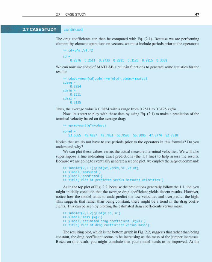
We can plot these values versus the actual measured terminal velocities. We will also superimpose a line indicating exact predictions (the 1:1 line) to help assess the results. Because we are going to eventually generate a second plot, we employ the subplot command:
>> subplot(2,1,1);plot(vt,vpred,'o',vt,vt)>> xlabel('measured')>> ylabel('predicted')>> title('Plot of predicted versus measured velocities')
As in the top plot of Fig. 2.2, because the predictions generally follow the 1:1 line, you might initially conclude that the average drag coefficient yields decent results. However, notice how the model tends to underpredict the low velocities and overpredict the high. This suggests that rather than being constant, there might be a trend in the drag coeffi-cients. This can be seen by plotting the estimated drag coefficients versus mass:
>> subplot(2,1,2);plot(m,cd,'o')>> xlabel('mass (kg)')>> ylabel('estimated drag coefficient (kg/m)')>> title('Plot of drag coefficient versus mass')
The resulting plot, which is the bottom graph in Fig. 2.2, suggests that rather than being constant, the drag coefficient seems to be increasing as the mass of the jumper increases. Based on this result, you might conclude that your model needs to be improved. At the
cha97962_ch02_027-052.indd 47 08/11/16 3:21 pm

48 MATLAB FundAMenTALs
2.7 CASE STUDY continued
least, it might motivate you to conduct further experiments with a larger number of jumpers to confirm your preliminary finding.
In addition, the result might also stimulate you to go to the fluid mechanics literature and learn more about the science of drag. As described previously in Sec. 1.4, you would discover that the parameter cd is actually a lumped drag coefficient that along with the true drag includes other factors such as the jumper’s frontal area and air density:
cd = CD ρ A
_____ 2 (2.2)
where CD = a dimensionless drag coefficient, ρ = air density (kg/m3), and A = frontal area (m2), which is the area projected on a plane normal to the direction of the velocity.
Assuming that the densities were relatively constant during data collection (a pretty good assumption if the jumpers all took off from the same height on the same day), Eq. (2.2) suggests that heavier jumpers might have larger areas. This hypothesis could be substanti-ated by measuring the frontal areas of individuals of varying masses.
FIGURE 2.2Two plots created with MATLAB.
60Plot of predicted versus measured velocities
Measured
Pred
icte
d 55
50
4547 48 49 50 51 52 53 54 55 56
0.35Plot of drag coe�cient versus mass
Mass (kg)
Estim
ated
dra
gco
e�ci
ent (
kg/m
)
0.3
0.25
0.260 65 70 75 80 85 90 95
cha97962_ch02_027-052.indd 48 08/11/16 3:21 pm
prOBLeMs 49
PROBLEMS
2.1 What is the output when the following commands are implemented?A = [1:3;2:2:6;3:−1:1]A = A'A(:,3) = []A = [A(:,1) [4 5 7]' A(:,2)]A = sum(diag(A))2.2 You want to write MATLAB equations to compute a vector of y values using the following equations
(a) y = 6t3 − 3t − 4 _______ 8 sin(5t)
(b) y = 6t − 4 ______ 8t − π __ 2 t
where t is a vector. Make sure that you use periods only where necessary so the equation handles vector operations properly. Extra periods will be considered incorrect.2.3 Write a MATLAB expression to compute and dis-play the values of a vector of x values using the following equation
x = y (a + bz)1.8 __________ z(1 − y)
Assume that y and z are vector quantities of equal length and a and b are scalars. 2.4 What is displayed when the following MATLAB state-ments are executed?(a) A = [1 2; 3 4; 5 6]; A(2,:)'(b) y = [0:1.5:7]'(c) a = 2; b = 8; c = 4; a + b / c2.5 The MATLAB humps function defines a curve that has 2 maxima (peaks) of unequal height over the interval 0 ≤ x ≤ 2,
f (x) = 1 ______________ (x − 0.3)2 + 0.01
+ 1 ______________ (x − 0.9)2 + 0.04
− 6
Use MATLAB to generate a plot of f (x) versus x withx = [0:1/256:2];
Do not use MATLAB’s built-in humps function to generate the values of f (x). Also, employ the minimum number of periods to perform the vector operations needed to generate f (x) values for the plot.2.6 Use the linspace function to create vectors identical to the following created with colon notation:(a) t = 4:6:35(b) x = −4:22.7 Use colon notation to create vectors identical to the following created with the linspace function:(a) v = linspace(−2,1.5,8)(b) r = linspace(8,4.5,8)
2.8 The command linspace(a, b, n) generates a row vec-tor of n equally spaced points between a and b. Use colon notation to write an alternative one-line command to gener-ate the same vector. Test your formulation for a = −3, b = 5, n = 6. 2.9 The following matrix is entered in MATLAB:
>> A = [3 2 1;0:0.5:1;linspace(6, 8, 3)]
(a) Write out the resulting matrix.(b) Use colon notation to write a single-line MATLAB
command to multiply the second row by the third col-umn and assign the result to the variable c.
2.10 The following equation can be used to compute values of y as a function of x:
y = be−ax sin(bx) (0.012x4 − 0.15x3 + 0.075x2 + 2.5x)
where a and b are parameters. Write the equation for imple-mentation with MATLAB, where a = 2, b = 5, and x is a vector holding values from 0 to π∕2 in increments of Δx = π∕40. Employ the minimum number of periods (i.e., dot no-tation) so that your formulation yields a vector for y. In ad-dition, compute the vector z = y2 where each element holds the square of each element of y. Combine x, y, and z into a matrix w, where each column holds one of the variables, and display w using the short g format. In addition, gener-ate a labeled plot of y and z versus x. Include a legend on the plot (use help to understand how to do this). For y, use a 1.5-point, dashdotted red line with 14-point, red-edged, white-faced pentagram-shaped markers. For z, use a stan-dard-sized (i.e., default) solid blue line with standard-sized, blue-edged, green-faced square markers.2.11 A simple electric circuit consisting of a resistor, a ca-pacitor, and an inductor is depicted in Fig. P2.11. The charge on the capacitor q(t) as a function of time can be computed as
q(t) = q0e−Rt∕(2L) cos [ √__________
1 ___ LC − ( R ___ 2L ) 2 t ] where t = time, q0 the initial charge, R = the resistance, L = inductance, and C = capacitance. Use MATLAB to generate a plot of this function from t = 0 to 0.8, given that q0 = 10, R = 60, L = 9, and C = 0.00005.2.12 The standard normal probability density function is a bell-shaped curve that can be represented as
f (z) = 1 _____ √
___ 2π e−z2∕2
cha97962_ch02_027-052.indd 49 08/11/16 3:21 pm

50 MATLAB FundAMenTALs
Use MATLAB to generate a plot of this function from z = −5 to 5. Label the ordinate as frequency and the abscissa as z.2.13 If a force F (N) is applied to compress a spring, its displacement x (m) can often be modeled by Hooke’s law:
F = kx
where k = the spring constant (N/m). The potential energy stored in the spring U (J) can then be computed as
U = 1 __ 2 kx2
Five springs are tested and the following data compiled:
F, N 14 18 8 9 13x, m 0.013 0.020 0.009 0.010 0.012
Use MATLAB to store F and x as vectors and then compute vectors of the spring constants and the potential energies. Use the max function to determine the maximum potential energy.2.14 The density of freshwater can be computed as a func-tion of temperature with the following cubic equation:
ρ = 5.5289 × 10⁻⁸ T C 3 − 8.5016 × 10⁻⁶ T C 2
+ 6.5622 × 10⁻⁵TC + 0.99987
where ρ = density (g/cm3) and TC = temperature (°C). Use MATLAB to generate a vector of temperatures ranging from 32 °F to 93.2 °F using increments of 3.6 °F. Convert this vector to degrees Celsius and then compute a vector of den-sities based on the cubic formula. Create a plot of ρ versus TC. Recall that TC = 5/9(TF − 32).2.15 Manning’s equation can be used to compute the veloc-ity of water in a rectangular open channel:
U = √__
S ____ n ( BH _______ B + 2H ) 2∕3
where U = velocity (m/s), S = channel slope, n = roughness coefficient, B = width (m), and H = depth (m). The follow-ing data are available for five channels:
n S B H
0.035 0.0001 10 20.020 0.0002 8 10.015 0.0010 20 1.50.030 0.0007 24 30.022 0.0003 15 2.5
Store these values in a matrix where each row represents one of the channels and each column represents one of the param-eters. Write a single-line MATLAB statement to compute a column vector containing the velocities based on the values in the parameter matrix.2.16 It is general practice in engineering and science that equations be plotted as lines and discrete data as symbols. Here are some data for concentration (c) versus time (t) for the photodegradation of aqueous bromine:
t, min 10 20 30 40 50 60c, ppm 3.4 2.6 1.6 1.3 1.0 0.5
These data can be described by the following function:
c = 4.84e−0.034t
Use MATLAB to create a plot displaying both the data (using diamond-shaped, filled-red symbols) and the func-tion (using a green, dashed line). Plot the function for t = 0 to 70 min.2.17 The semilogy function operates in an identical fashion to the plot function except that a logarithmic (base-10) scale is used for the y axis. Use this function to plot the data and function as described in Prob. 2.16. Explain the results.2.18 Here are some wind tunnel data for force (F) versus velocity (υ):
υ, m/s 10 20 30 40 50 60 70 80F, N 25 70 380 550 610 1220 830 1450
These data can be described by the following function:
F = 0.2741υ1.9842
Switch
Resistor
Capacitor−
+V0
i−
+Battery Inductor
FIGURE P2.11
cha97962_ch02_027-052.indd 50 08/11/16 3:21 pm
prOBLeMs 51
(b) >> q = 4:2:12; >> r = [7 8 4; 3 6 –5]; >> sum(q) * r(2, 3) 2.24 The trajectory of an object can be modeled as
y = (tan θ0)x − g ________ 2 υ 0
2 cos2θ0
x2 + y0
where y = height (m), θ0 = initial angle (radians), x = horizontal distance (m), g = gravitational acceleration (= 9.81 m/s2), υ0 = initial velocity (m/s), and y0 = initial height. Use MATLAB to find the trajectories for y0 = 0 and υ0 = 28 m/s for initial angles ranging from 15 to 75° in incre-ments of 15°. Employ a range of horizontal distances from x = 0 to 80 m in increments of 5 m. The results should be as-sembled in an array where the first dimension (rows) corre-sponds to the distances, and the second dimension (columns) corresponds to the different initial angles. Use this matrix to generate a single plot of the heights versus horizontal distances for each of the initial angles. Employ a legend to distinguish among the different cases, and scale the plot so that the minimum height is zero using the axis command.2.25 The temperature dependence of chemical reactions can be computed with the Arrhenius equation:
k = Ae−E∕(RTa)
where k = reaction rate (s−1), A = the preexponential (or fre-quency) factor, E = activation energy (J/mol), R = gas con-stant [8.314 J/(mole · K)], and Ta = absolute temperature (K). A compound has E = 1 × 10⁵ J/mol and A = 7 × 10¹⁶. Use MATLAB to generate values of reaction rates for temperatures ranging from 253 to 325 K. Use subplot to gen-erate a side-by-side graph of (a) k versus Ta (green line) and (b) log10 k (red line) versus 1∕Ta. Employ the semilogy func-tion to create (b). Include axis labels and titles for both sub-plots. Interpret your results.2.26 Figure P2.26a shows a uniform beam subject to a lin-early increasing distributed load. As depicted in Fig. P2.26b, deflection y (m) can be computed with
y = w0 _______ 120EIL (−x5 + 2L2x3 − L4x)
where E = the modulus of elasticity and I = the moment of inertia (m4). Employ this equation and calculus to generate MATLAB plots of the following quantities versus distance along the beam: (a) displacement (y), (b) slope [θ (x) = dy/dx], (c) moment [M(x) = EId2 y/dx2], (d) shear [V(x) = EId3 y/dx3], and (e) loading [w(x) = −EId 4 y/dx4].
Use MATLAB to create a plot displaying both the data (using circular magenta symbols) and the function (using a black dash-dotted line). Plot the function for υ = 0 to 100 m/s and label the plot’s axes.2.19 The loglog function operates in an identical fash-ion to the plot function except that logarithmic scales are used for both the x and y axes. Use this function to plot the data and function as described in Prob. 2.18. Explain the results.2.20 The Maclaurin series expansion for the cosine is
cos x = 1 − x2 __ 2! + x
4 __ 4! − x
6 __ 6! + x
8 __ 8! − · · ·
Use MATLAB to create a plot of the cosine (solid line) along with a plot of the series expansion (black dashed line) up to and including the term x8∕8!. Use the built-in func-tion factorial in computing the series expansion. Make the range of the abscissa from x = 0 to 3π∕2.2.21 You contact the jumpers used to generate the data in Table 2.1 and measure their frontal areas. The result-ing values, which are ordered in the same sequence as the corresponding values in Table 2.1, are
A, m2 0.455 0.402 0.452 0.486 0.531 0.475 0.487
(a) If the air density is ρ = 1.223 kg/m3, use MATLAB to compute values of the dimensionless drag coefficient CD.
(b) Determine the average, minimum, and maximum of the resulting values.
(c) Develop a stacked plot of A versus m (upper) and CD versus m (lower). Include descriptive axis labels and titles on the plots.
2.22 The following parametric equations generate a conical helix.
x = t cos(6t)y = t sin(6t)z = t
Compute values of x, y, and z for t = 0 to 6π with Δt = π/64. Use subplot to generate a two-dimensional line plot (red solid line) of (x, y) in the top pane and a three-dimensional line plot (cyan solid line) of (x, y, z) in the bottom pane. Label the axes for both plots.2.23 Exactly what will be displayed after the following MATLAB commands are typed?(a) >> x = 5; >> x ^ 3; >> y = 8 – x
cha97962_ch02_027-052.indd 51 08/11/16 3:21 pm

52 MATLAB FundAMenTALs
Use the following parameters for your computation: L = 600 cm, E = 50,000 kN/cm2, I = 30,000 cm4, w0 = 2.5 kN/cm, and Δx = 10 cm. Employ the subplot function to display all the plots vertically on the same page in the order (a) to (e).
Include labels and use consistent MKS units when developing the plots.2.27 The butterfly curve is given by the following paramet-ric equations:
x = sin(t) ( ecos t − 2 cos 4t − sin5 t ___ 12 )
y = cos(t) ( ecos t − 2 cos 4t − sin5 t ___ 12 ) Generate values of x and y for values of t from 0 to 100 with Δt = 1/16. Construct plots of (a) x and y versus t and (b) y versus x. Use subplot to stack these plots vertically and make the plot in (b) square. Include titles and axis labels on both plots and a legend for (a). For (a), employ a dotted line for y in order to distinguish it from x.2.28 The butterfly curve from Prob. 2.27 can also be repre-sented in polar coordinates as
r = esin θ − 2 cos(4θ ) − sin5 ( 2θ − π ______ 24 ) Generate values of r for values of θ from 0 to 8π with Δθ = π /32. Use the MATLAB function polar to generate the polar plot of the butterfly curve with a dashed red line. Employ the MATLAB Help to understand how to generate the plot.
w0
L(a)
(x = 0, y = 0)(x = L, y = 0)
x
(b)
FIGURE P2.26
cha97962_ch02_027-052.indd 52 08/11/16 3:21 pm

53
CHAPTER OBJECTIVES
The primary objective of this chapter is to learn how to write M-file programs to implement numerical methods. Specific objectives and topics covered are
• Learning how to create well-documented M-files in the edit window and invoke them from the command window.
• Understanding how script and function files differ.• Understanding how to incorporate help comments in functions.• Knowing how to set up M-files so that they interactively prompt users for
information and display results in the command window.• Understanding the role of subfunctions and how they are accessed.• Knowing how to create and retrieve data files.• Learning how to write clear and well-documented M-files by employing
structured programming constructs to implement logic and repetition.• Recognizing the difference between if...elseif and switch constructs.• Recognizing the difference between for...end and while structures.• Knowing how to animate MATLAB plots.• Understanding what is meant by vectorization and why it is beneficial.• Understanding how anonymous functions can be employed to pass functions to
function function M-files.
3Programming with MATLAB
YOU’VE GOT A PROBLEM
In Chap. 1, we used a force balance to develop a mathematical model to predict the fall velocity of a bungee jumper. This model took the form of the following differential equation:
dυ ___ dt = g − cd __ m υ∣υ∣
cha97962_ch03_053-098.indd 53 08/11/16 3:22 pm

54 ProgrAMMIng wITh MATLAB
We also learned that a numerical solution of this equation could be obtained with Euler’s method:
υi+1 = υi + dυi ___ dt Δt
This equation can be implemented repeatedly to compute velocity as a function of time. However, to obtain good accuracy, many small steps must be taken. This would be extremely laborious and time consuming to implement by hand. However, with the aid of MATLAB, such calculations can be performed easily.
So our problem now is to figure out how to do this. This chapter will introduce you to how MATLAB M-files can be used to obtain such solutions.
3.1 M-FILES
The most common way to operate MATLAB is by entering commands one at a time in the command window. M-files provide an alternative way of performing operations that greatly expand MATLAB’s problem-solving capabilities. An M-file consists of a series of statements that can be run all at once. Note that the nomenclature “M-file” comes from the fact that such files are stored with a .m extension. M-files come in two flavors: script files and function files.
3.1.1 Script Files
A script file is merely a series of MATLAB commands that are saved on a file. They are useful for retaining a series of commands that you want to execute on more than one oc-casion. The script can be executed by typing the file name in the command window or by pressing the Run button.
EXAMPLE 3.1 Script File
Problem Statement. Develop a script file to compute the velocity of the free-falling bun-gee jumper for the case where the initial velocity is zero.
Solution. Open the editor with the selection: New, Script. Type in the following state-ments to compute the velocity of the free-falling bungee jumper at a specific time [recall Eq. (1.9)]:
g = 9.81; m = 68.1; t = 12; cd = 0.25;v = sqrt(g * m / cd) * tanh(sqrt(g * cd / m) * t)
Save the file as scriptdemo.m. Return to the command window and type
>>scriptdemo
The result will be displayed as
v = 50.6175
Thus, the script executes just as if you had typed each of its lines in the command window.
cha97962_ch03_053-098.indd 54 08/11/16 3:22 pm
3.1 M-FILES 55
As a final step, determine the value of g by typing>> g
g = 9.8100
So you can see that even though g was defined within the script, it retains its value back in the command workspace. As we will see in the following section, this is an important distinction between scripts and functions.
3.1.2 Function Files
Function files are M-files that start with the word function. In contrast to script files, they can accept input arguments and return outputs. Hence they are analogous to user- defined functions in programming languages such as Fortran, Visual Basic or C.
The syntax for the function file can be represented generally as
function outvar = funcname(arglist)% helpcommentsstatementsoutvar = value;
where outvar = the name of the output variable, funcname = the function’s name, arglist = the function’s argument list (i.e., comma-delimited values that are passed into the function), helpcomments = text that provides the user with information regarding the function (these can be invoked by typing Help funcname in the command window), and statements = MATLAB statements that compute the value that is assigned to outvar.
Beyond its role in describing the function, the first line of the helpcomments, called the H1 line, is the line that is searched by the lookfor command (recall Sec. 2.6). Thus, you should include key descriptive words related to the file on this line.
The M-file should be saved as funcname.m. The function can then be run by typing funcname in the command window as illustrated in the following example. Note that even though MATLAB is case-sensitive, your computer’s operating system may not be. Whereas MATLAB would treat function names like freefall and FreeFall as two different variables, your operating system might not.
EXAMPLE 3.2 Function File
Problem Statement. As in Example 3.1, compute the velocity of the free-falling bungee jumper but now use a function file for the task.
Solution. Type the following statements in the file editor:
function v = freefall(t, m, cd)% freefall: bungee velocity with second-order drag% v=freefall(t,m,cd) computes the free-fall velocity% of an object with second-order drag% input:
cha97962_ch03_053-098.indd 55 08/11/16 3:22 pm
56 ProgrAMMIng wITh MATLAB
% t = time (s)% m = mass (kg)% cd = second-order drag coefficient (kg/m)% output:% v = downward velocity (m/s)
g = 9.81; % acceleration of gravityv = sqrt(g * m / cd)*tanh(sqrt(g * cd / m) * t);
Save the file as freefall.m. To invoke the function, return to the command window and type in
>> freefall(12,68.1,0.25)
The result will be displayed as
ans = 50.6175
One advantage of a function M-file is that it can be invoked repeatedly for different argument values. Suppose that you wanted to compute the velocity of a 100-kg jumper after 8 s:
>> freefall(8,100,0.25)
ans = 53.1878
To invoke the help comments type
>> help freefall
which results in the comments being displayed
freefall: bungee velocity with second-order drag v = freefall(t,m,cd) computes the free-fall velocity of an object with second-order draginput: t = time (s) m = mass (kg) cd = second-order drag coefficient (kg/m)output: v = downward velocity (m/s)
If at a later date, you forgot the name of this function, but remembered that it involved bungee jumping, you could enter
>> lookfor bungee
and the following information would be displayed
freefall.m − bungee velocity with second-order drag
Note that, at the end of the previous example, if we had typed>> g
cha97962_ch03_053-098.indd 56 08/11/16 3:22 pm

3.1 M-FILES 57
the following message would have been displayed
??? Undefined function or variable 'g'.
So even though g had a value of 9.81 within the M-file, it would not have a value in the command workspace. As noted previously at the end of Example 3.1, this is an important distinction between functions and scripts. The variables within a function are said to be local and are erased after the function is executed. In contrast, the variables in a script retain their existence after the script is executed.
Function M-files can return more than one result. In such cases, the variables containing the results are comma-delimited and enclosed in brackets. For example, the following function, stats.m, computes the mean and the standard deviation of a vector:
function [mean, stdev] = stats(x)n = length(x);mean = sum(x)/n;stdev = sqrt(sum((x-mean).^2/(n − 1)));
Here is an example of how it can be applied:
>> y = [8 5 10 12 6 7.5 4];>> [m,s] = stats(y)
m = 7.5000
s = 2.8137
Although we will also make use of script M-files, function M-files will be our primary programming tool for the remainder of this book. Hence, we will often refer to function M-files as simply M-files.
3.1.3 Variable Scope
MATLAB variables have a property known as scope that refers to the context of the com-puting environment in which the variable has a unique identity and value. Typically, a variable’s scope is limited either to the MATLAB workspace or within a function. This principle prevents errors when a programmer unintentionally gives the same name to vari-ables in different contexts.
Any variables defined through the command line are within the MATLAB workspace and you can readily inspect a workspace variable’s value by entering its name at the com-mand line. However, workspace variables are not directly accessible to functions but rather are passed to functions via their arguments. For example, here is a function that adds two numbers
function c = adder(a,b)x = 88ac = a + b
cha97962_ch03_053-098.indd 57 08/11/16 3:22 pm

58 ProgrAMMIng wITh MATLAB
Suppose in the command window we type
>> x = 1; y = 4; c = 8c = 8
So as expected, the value of c in the workspace is 8. If you type >> d = adder(x,y)
the result will be
x = 88a = 1c = 5d = 5
But, if you then type>> c, x, a
The result is
c = 8x = 1
Undefined function or variable 'a'.Error in ScopeScript (line 6)c, x, a
The point here is that even though x was assigned a new value inside the function, the variable of the same name in the MATLAB workspace is unchanged. Even though they have the same name, the scope of each is limited to their context and does not overlap. In the function, the variables a and b are limited in scope to that function, and only exist while that function is being executed. Such variables are formally called local variables. Thus, when we try to display the value of a in the workspace, an error message is generated be-cause the workspace has no access to the a in the function.
Another obvious consequence of limited-scope variables is that any parameter needed by a function must be passed as an input argument or by some other explicit means. A func-tion cannot otherwise access variables in the workspace or in other functions.
3.1.4 Global Variables
As we have just illustrated, the function’s argument list is like a window through which information is selectively passed between the workspace and a function, or between two functions. Sometimes, however, it might be convenient to have access to a vari-able in several contexts without passing it as an argument. In such cases, this can be
cha97962_ch03_053-098.indd 58 08/11/16 3:22 pm

3.1 M-FILES 59
accomplished by defining the variable as global. This is done with the global command, which is defined as
global X Y Z
where X, Y, and Z are global in scope. If several functions (and possibly the workspace), all declare a particular name as global, then they all share a single value of that variable. Any change to that variable, in any function, is then made to all the other functions that declare it global. Stylistically, MATLAB recommends that global variables use all capital letters, but this is not required.
EXAMPLE 3.3 Use of global Variables
Problem Statement. The Stefan-Boltzmann law is used to compute the radiation flux from a black body1 as in
J = σ T a 4
where J = radiation flux [W/(m2 s)], σ = the Stefan-Boltzmann constant (5.670367 × 10⁻⁸ W m−2 K−4), and Ta = absolute temperature (K). In assessing the impact of climate change on water temperature, it is used to compute the radiation terms in a waterbody’s heat balance. For example, the long-wave radiation from the atmosphere to the waterbody, Jan [W/(m2 s)], can be calculated as
Jan = 0.97σ(Tair + 273.15)4 ( 0.6 + 0.031 √___
eair ) where Tair = the temperature of the air above the waterbody (°C), and eair = the vapor pres-sure of the air above the water body (mmHg),
eair = 4.596e 17.27 T d _ 237.3 + T d (E3.3.1)
where Td = the dew-point temperature (°C). The radiation from the water surface back into the atmosphere, Jbr [W/(m2 s)], is calculated as
Jbr = 0.97σ(Tw + 273.15)4 (E3.3.2)
where Tw = the water temperature (°C). Write a script that utilizes two functions to com-pute the net long-wave radiation (i.e., the difference between the atmospheric radiation in and the water back radiation out) for a cold lake with a surface temperature of Tw = 15 °C on a hot (Tair = 30 °C), humid (Td = 27.7 °C) summer day. Use global to share the Stefan-Boltzmann constant between the script and functions.
Solution. Here is the script
clc, format compactglobal SIGMASIGMA = 5.670367e−8;Tair = 30; Tw = 15; Td = 27.7;
1A black body is an object that absorbs all incident electromagnetic radiation, regardless of frequency or angle of incidence. A white body is one that reflects all incident rays completely and uniformly in all directions.
cha97962_ch03_053-098.indd 59 08/11/16 3:22 pm

60 ProgrAMMIng wITh MATLAB
Jan = AtmLongWaveRad(Tair, Td)Jbr = WaterBackRad(Tw)JnetLongWave = Jan −Jbr
Here is a function to compute the incoming long wave radiation from the atmosphere into the lake
function Ja = AtmLongWaveRad(Tair, Td)global SIGMAeair = 4.596*exp(17.27*Td/(237.3+Td));Ja = 0.97*SIGMA*(Tair+273.15)^4*(0.6+0.031*sqrt(eair));end
and here is a function to compute the long wave radiation from the lake back into the atmosphere
function Jb = WaterBackRad(Twater)global SIGMAJb = 0.97*SIGMA*(Twater+273.15)^4;end
When the script is run, the output is
Jan = 354.8483Jbr = 379.1905JnetLongWave = −24.3421
Thus, for this case, because the back radiation is larger than the incoming radiation, so the lake loses heat at the rate of 24.3421 W/(m2 s) due to the two long-wave radiation fluxes.
If you require additional information about global variables, you can always type help global at the command prompt. The help facility can also be invoked to learn about other MATLAB commands dealing with scope such as persistent.
3.1.5 Subfunctions
Functions can call other functions. Although such functions can exist as separate M-files, they may also be contained in a single M-file. For example, the M-file in Example 3.2 (without comments) could have been split into two functions and saved as a single M-file2:
function v = freefallsubfunc(t, m, cd)v = vel(t, m, cd);end
function v = vel(t, m, cd)g = 9.81;v = sqrt(g * m / cd)*tanh(sqrt(g * cd / m) * t);end
2Note that although end statements are not used to terminate single-function M-files, they are included when subfunctions are involved to demarcate the boundaries between the main function and the subfunctions.
cha97962_ch03_053-098.indd 60 08/11/16 3:22 pm
3.2 InPUT-oUTPUT 61
This M-file would be saved as freefallsubfunc.m. In such cases, the first function is called the main or primary function. It is the only function that is accessible to the command win-dow and other functions and scripts. All the other functions (in this case, vel) are referred to as subfunctions.
A subfunction is only accessible to the main function and other subfunctions within the M-file in which it resides. If we run freefallsubfunc from the command window, the result is identical to Example 3.2:
>> freefallsubfunc(12,68.1,0.25)
ans = 50.6175
However, if we attempt to run the subfunction vel, an error message occurs:
>> vel(12,68.1,.25)??? Undefined function or method 'vel' for input arguments of type 'double'.
3.2 INPUT-OUTPUT
As in Sec.3.1, information is passed into the function via the argument list and is output via the function’s name. Two other functions provide ways to enter and display information directly using the command window.
The input Function. This function allows you to prompt the user for values directly from the command window. Its syntax is
n = input('promptstring')
The function displays the promptstring, waits for keyboard input, and then returns the value from the keyboard. For example,
m = input('Mass (kg): ')
When this line is executed, the user is prompted with the message
Mass (kg):
If the user enters a value, it would then be assigned to the variable m.The input function can also return user input as a string. To do this, an 's' is appended
to the function’s argument list. For example,
name = input('Enter your name: ','s')
The disp Function. This function provides a handy way to display a value. Its syntax is
disp(value)
where value = the value you would like to display. It can be a numeric constant or vari-able, or a string message enclosed in hyphens. Its application is illustrated in the following example.
cha97962_ch03_053-098.indd 61 08/11/16 3:22 pm

62 ProgrAMMIng wITh MATLAB
EXAMPLE 3.4 An Interactive M-File Function
Problem Statement. As in Example 3.2, compute the velocity of the free-falling bungee jumper, but now use the input and disp functions for input/output.
Solution. Type the following statements in the file editor:
function freefalli% freefalli: interactive bungee velocity% freefalli interactive computation of the% free-fall velocity of an object% with second-order drag.g = 9.81; % acceleration of gravitym = input('Mass (kg): ');cd = input('Drag coefficient (kg/m): ');t = input('Time (s): ');disp(' ')disp(‘Velocity (m/s):')disp(sqrt(g * m / cd)*tanh(sqrt(g * cd / m) * t))
Save the file as freefalli.m. To invoke the function, return to the command window and type >> freefalli
Mass (kg): 68.1Drag coefficient (kg/m): 0.25Time (s): 12
Velocity (m/s): 50.6175
The fprintf Function. This function provides additional control over the display of information. A simple representation of its syntax is
fprintf('format', x, ...)
where format is a string specifying how you want the value of the variable x to be displayed. The operation of this function is best illustrated by examples.
A simple example would be to display a value along with a message. For instance, suppose that the variable velocity has a value of 50.6175. To display the value using eight digits with four digits to the right of the decimal point along with a message, the statement along with the resulting output would be
>> fprintf('The velocity is %8.4f m/s\n', velocity)
The velocity is 50.6175 m/s
This example should make it clear how the format string works. MATLAB starts at the left end of the string and displays the labels until it detects one of the symbols: % or \. In our example, it first encounters a % and recognizes that the following text is a format code. As in Table 3.1, the format codes allow you to specify whether numeric values are displayed in integer, decimal, or scientific format. After displaying the value of velocity, MATLAB continues displaying the character information (in our case the units: m/s) until it detects the symbol \. This tells MATLAB that the following text is a control code. As in Table 3.1, the
cha97962_ch03_053-098.indd 62 08/11/16 3:22 pm

3.2 InPUT-oUTPUT 63
control codes provide a means to perform actions such as skipping to the next line. If we had omitted the code \n in the previous example, the command prompt would appear at the end of the label m/s rather than on the next line as would typically be desired.
The fprintf function can also be used to display several values per line with different formats. For example,
>> fprintf('%5d %10.3f %8.5e\n',100,2*pi,pi);
100 6.283 3.14159e + 000
It can also be used to display vectors and matrices. Here is an M-file that enters two sets of values as vectors. These vectors are then combined into a matrix, which is then displayed as a table with headings:
function fprintfdemox = [1 2 3 4 5];y = [20.4 12.6 17.8 88.7 120.4];z = [x;y];fprintf(' x y\n');fprintf('%5d %10.3f\n',z);
The result of running this M-file is
>> fprintfdemo
x y 1 20.400 2 12.600 3 17.800 4 88.700 5 120.400
3.2.1 Creating and Accessing Files
MATLAB has the capability to both read and write data files. The simplest approach in-volves a special type of binary file, called a MAT-file, which is expressly designed for implementation within MATLAB. Such files are created and accessed with the save and load commands.
TABLE 3.1 Commonly used format and control codes employed with the fprintf function.
Format Code Description
%d Integer format%e Scientific format with lowercase e%E Scientific format with uppercase E%f Decimal format%g The more compact of %e or %f
Control Code Description
\n Start new line\t Tab
cha97962_ch03_053-098.indd 63 08/11/16 3:22 pm

64 ProgrAMMIng wITh MATLAB
The save command can be used to generate a MAT-file holding either the entire work-space or a few selected variables. A simple representation of its syntax is
save filename var1 var2 ... varn
This command creates a MAT-file named filename.mat that holds the variables var1 through varn. If the variables are omitted, all the workspace variables are saved. The load command can subsequently be used to retrieve the file:
load filename var1 var2 ... varn
which retrieves the variables var1 through varn from filename.mat. As was the case with save, if the variables are omitted, all the variables are retrieved.
For example, suppose that you use Eq. (1.9) to generate velocities for a set of drag coefficients:
>> g = 9.81;m = 80;t = 5;>> cd = [.25 .267 .245 .28 .273]';>> v = sqrt(g*m ./cd).*tanh(sqrt(g*cd/m)*t);
You can then create a file holding the values of the drag coefficients and the velocities with
>> save veldrag v cd
To illustrate how the values can be retrieved at a later time, remove all variables from the workspace with the clear command,
>> clear
At this point, if you tried to display the velocities you would get the result:
>> v??? Undefined function or variable 'v'.
However, you can recover them by entering
>> load veldrag
Now, the velocities are available as can be verified by typing
>> who
Your variables are:cd v
Although MAT-files are quite useful when working exclusively within the MATLAB environment, a somewhat different approach is required when interfacing MATLAB with other programs. In such cases, a simple approach is to create text files written in ASCII format.
ASCII files can be generated in MATLAB by appending –ascii to the save command. In contrast to MAT-files where you might want to save the entire workspace, you would typically save a single rectangular matrix of values. For example,
>> A = [5 7 9 2;3 6 3 9];>> save simpmatrix.txt –ascii
cha97962_ch03_053-098.indd 64 08/11/16 3:22 pm
3.3 STrUCTUrED ProgrAMMIng 65
In this case, the save command stores the values in A in 8-digit ASCII form. If you want to store the numbers in double precision, just append –ascii –double. In either case, the file can be accessed by other programs such as spreadsheets or word processors. For example, if you open this file with a text editor, you will see5.0000000e + 000 7.0000000e + 000 9.0000000e + 000 2.0000000e + 0003.0000000e + 000 6.0000000e + 000 3.0000000e + 000 9.0000000e + 000
Alternatively, you can read the values back into MATLAB with the load command,>> load simpmatrix.txt
Because simpmatrix.txt is not a MAT-file, MATLAB creates a double precision array named after the filename:
>> simpmatrix
simpmatrix = 5 7 9 2 3 6 3 9
Alternatively, you could use the load command as a function and assign its values to a variable as in
>> A = load('simpmatrix.txt')
The foregoing material covers but a small portion of MATLAB’s file management capabilities. For example, a handy import wizard can be invoked with the menu selections: File, Import Data. As an exercise, you can demonstrate the import wizards convenience by using it to open simpmatrix.txt. In addition, you can always consult help to learn more about this and other features.
3.3 STRUCTURED PROGRAMMING
The simplest of all M-files perform instructions sequentially. That is, the program state-ments are executed line by line starting at the top of the function and moving down to the end. Because a strict sequence is highly limiting, all computer languages include state-ments allowing programs to take nonsequential paths. These can be classified as
• Decisions (or Selection). The branching of flow based on a decision.• Loops (or Repetition). The looping of flow to allow statements to be repeated.
3.3.1 Decisions
The if Structure. This structure allows you to execute a set of statements if a logical condition is true. Its general syntax is
if condition statementsend
where condition is a logical expression that is either true or false. For example, here is a simple M-file to evaluate whether a grade is passing:
function grader(grade)% grader(grade):
cha97962_ch03_053-098.indd 65 08/11/16 3:22 pm

66 ProgrAMMIng wITh MATLAB
% determines whether grade is passing% input:% grade = numerical value of grade (0−100)% output:% displayed message if grade >= 60 disp('passing grade')end
The following illustrates the result>> grader(95.6)
passing grade
For cases where only one statement is executed, it is often convenient to implement the if structure as a single line,
if grade > 60, disp('passing grade'), end
This structure is called a single-line if. For cases where more than one statement is imple-mented, the multiline if structure is usually preferable because it is easier to read.
Error Function. A nice example of the utility of a single-line if is to employ it for rudi-mentary error trapping. This involves using the error function which has the syntax,
error(msg)
When this function is encountered, it displays the text message msg, indicates where the error occurred, and causes the M-file to terminate and return to the command window.
An example of its use would be where we might want to terminate an M-file to avoid a division by zero. The following M-file illustrates how this could be done:
function f = errortest(x)if x == 0, error('zero value encountered'), endf = 1/x;
If a nonzero argument is used, the division would be implemented successfully as in>> errortest(10)
ans = 0.1000
However, for a zero argument, the function would terminate prior to the division and the error message would be displayed in red typeface:
>> errortest(0)
??? Error using ==> errortest at 2zero value encountered
Logical Conditions. The simplest form of the condition is a single relational expression that compares two values as in
value1 relation value2
where the values can be constants, variables, or expressions and the relation is one of the relational operators listed in Table 3.2.
cha97962_ch03_053-098.indd 66 08/11/16 3:22 pm

3.3 STrUCTUrED ProgrAMMIng 67
MATLAB also allows testing of more than one logical condition by employing logical operators. We will emphasize the following:
• ~(Not). Used to perform logical negation on an expression. ~ expression
If the expression is true, the result is false. Conversely, if the expression is false, the result is true.
• & (And). Used to perform a logical conjunction on two expressions. expression1 & expression2
If both expressions evaluate to true, the result is true. If either or both expressions evaluates to false, the result is false.
• || (Or). Used to perform a logical disjunction on two expressions. expression1 || expression2
If either or both expressions evaluate to true, the result is true.Table 3.3 summarizes all possible outcomes for each of these operators. Just as for
arithmetic operations, there is a priority order for evaluating logical operations. These are from highest to lowest: ~, &, and ||. In choosing between operators of equal priority, MATLAB evaluates them from left to right. Finally, as with arithmetic operators, paren-theses can be used to override the priority order.
Let’s investigate how the computer employs the priorities to evaluate a logical expres-sion. If a = −1, b = 2, x = 1, and y = 'b', evaluate whether the following is true or false:
a * b > 0 & b = = 2 & x > 7 || ~(y > 'd')
TABLE 3.2 Summary of relational operators in MATLAB.
Example Operator Relationship
x = = 0 = = Equalunit ~ = 'm' ~ = Not equala < 0 < Less thans > t > Greater than3.9 < = a/3 <= Less than or equal tor >= 0 >= Greater than or equal to
TABLE 3.3 A truth table summarizing the possible outcomes for logical operators employed in MATLAB. The order of priority of the operators is shown at the top of the table.
Highest Lowestx y ~x x & y x || y
T T F T TT F F F TF T T F TF F T F F
cha97962_ch03_053-098.indd 67 08/11/16 3:22 pm

68 ProgrAMMIng wITh MATLAB
To make it easier to evaluate, substitute the values for the variables:−1 * 2 > 0 & 2 = = 2 & 1 > 7 || ~('b' > 'd')
The first thing that MATLAB does is to evaluate any mathematical expressions. In this example, there is only one: −1 * 2,
−2 > 0 & 2 == 2 & 1 > 7 || ~('b' > 'd')
Next, evaluate all the relational expressions−2 > 0 & 2 == 2 & 1 > 7 || ~('b' > 'd') F & T & F || ~ F
At this point, the logical operators are evaluated in priority order. Since the ~ has highest priority, the last expression (~F) is evaluated first to give
F & T & F || T
The & operator is evaluated next. Since there are two, the left-to-right rule is applied and the first expression (F & T) is evaluated:
F & F || T
The & again has highest priorityF || T
Finally, the || is evaluated as true. The entire process is depicted in Fig. 3.1.
a * b > 0 & b = = 2 & x > 7 || ~ ( y > ' d ' )
T
T
F
−1 * 2 > 0 & 2 = = 2 & 1 > 7 || ~ ( ' b ' > ' d ' )
F & T & F || ~F
F & F ||
Substitute constants
Evaluate mathematicalexpressions
Evaluate relationalexpressions
Evaluate compoundexpressions
T||
−2 > 0 & 2 = = 2 & 1 > 7 || ~ ( ' b ' > ' d ' )
FIGURE 3.1A step-by-step evaluation of a complex decision.
cha97962_ch03_053-098.indd 68 08/11/16 3:22 pm

3.3 STrUCTUrED ProgrAMMIng 69
The if...else Structure. This structure allows you to execute a set of statements if a logical condition is true and to execute a second set if the condition is false. Its general syntax is
if condition statements1else statements2end
The if...elseif Structure. It often happens that the false option of an if...else structure is another decision. This type of structure often occurs when we have more than two op-tions for a particular problem setting. For such cases, a special form of decision structure, the if...elseif has been developed. It has the general syntax
if condition1 statements1elseif condition2 statements2elseif condition3 statements3 · · ·else statementselseend
EXAMPLE 3.5 if Structures
Problem Statement. For a scalar, the built-in MATLAB sign function returns the sign of its argument (−1, 0, 1). Here’s a MATLAB session that illustrates how it works:
>> sign(25.6)
ans = 1
>> sign(−0.776)
ans = −1
>> sign(0)
ans = 0
Develop an M-file to perform the same function.
Solution. First, an if structure can be used to return 1 if the argument is positive:function sgn = mysign(x)% mysign(x) returns 1 if x is greater than zero.if x > 0 sgn = 1;end
cha97962_ch03_053-098.indd 69 08/11/16 3:22 pm
70 ProgrAMMIng wITh MATLAB
This function can be run as>> mysign(25.6)
ans = 1
Although the function handles positive numbers correctly, if it is run with a negative or zero argument, nothing is displayed. To partially remedy this shortcoming, an if...else structure can be used to display –1 if the condition is false:function sgn = mysign(x)% mysign(x) returns 1 if x is greater than zero.% −1 if x is less than or equal to zero.if x > 0 sgn = 1;else sgn = −1;end
This function can be run as>> mysign(−0.776)
ans = −1
Although the positive and negative cases are now handled properly, −1 is erroneously returned if a zero argument is used. An if...elseif structure can be used to incorporate this final case:function sgn = mysign(x)% mysign(x) returns 1 if x is greater than zero.% −1 if x is less than zero.% 0 if x is equal to zero.if x > 0 sgn = 1;elseif x < 0 sgn = −1;else sgn = 0;end
The function now handles all possible cases. For example,>> mysign(0)
ans = 0
The switch Structure. The switch structure is similar in spirit to the if...elseif structure. However, rather than testing individual conditions, the branching is based on the value of a single test expression. Depending on its value, different blocks of code are implemented. In addition, an optional block is implemented if the expression takes on none of the prescribed values. It has the general syntax
switch testexpression case value1
cha97962_ch03_053-098.indd 70 08/11/16 3:22 pm

3.3 STrUCTUrED ProgrAMMIng 71
statements1 case value2 statements2 . . . otherwise statementsotherwiseend
As an example, here is function that displays a message depending on the value of the string variable, grade.
grade = 'B';switch grade case 'A' disp('Excellent') case 'B' disp('Good') case 'C' disp('Mediocre') case 'D' disp('Whoops') case 'F' disp('Would like fries with your order?') otherwise disp('Huh!')end
When this code was executed, the message “Good” would be displayed.
Variable Argument List. MATLAB allows a variable number of arguments to be passed to a function. This feature can come in handy for incorporating default values into your functions. A default value is a number that is automatically assigned in the event that the user does not pass it to a function.
As an example, recall that earlier in this chapter, we developed a function free fall, which had three arguments:
v = freefall(t,m,cd)
Although a user would obviously need to specify the time and mass, they might not have a good idea of an appropriate drag coefficient. Therefore, it would be nice to have the pro-gram supply a value if they omitted it from the argument list.
MATLAB has a function called nargin that provides the number of input arguments supplied to a function by a user. It can be used in conjunction with decision structures like the if or switch constructs to incorporate default values as well as error messages into your functions. The following code illustrates how this can be done for freefall:
function v = freefall2(t, m, cd)% freefall2: bungee velocity with second-order drag% v = freefall2(t,m,cd) computes the free-fall velocity% of an object with second-order drag.% input:% t = time (s)% m = mass (kg)
cha97962_ch03_053-098.indd 71 08/11/16 3:22 pm
72 ProgrAMMIng wITh MATLAB
% cd = drag coefficient (default = 0.27 kg/m)% output:% v = downward velocity (m/s)switch nargin case 0 error('Must enter time and mass') case 1 error('Must enter mass') case 2 cd = 0.27;end g = 9.81; % acceleration of gravityv = sqrt(g * m / cd)*tanh(sqrt(g * cd / m) * t);
Notice how we have used a switch structure to either display error messages or set the default, depending on the number of arguments passed by the user. Here is a command window session showing the results:
>> freefall2(12,68.1,0.25)
ans = 50.6175
>> freefall2(12,68.1)
ans = 48.8747
>> freefall2(12)
??? Error using ==> freefall2 at 15Must enter mass
>> freefall2()
??? Error using ==> freefall2 at 13Must enter time and mass
Note that nargin behaves a little differently when it is invoked in the command window. In the command window, it must include a string argument specifying the function and it returns the number of arguments in the function. For example,
>> nargin('freefall2')
ans = 3
3.3.2 Loops
As the name implies, loops perform operations repetitively. There are two types of loops, depending on how the repetitions are terminated. A for loop ends after a specified number of repetitions. A while loop ends on the basis of a logical condition.
The for...end Structure. A for loop repeats statements a specific number of times. Its general syntax is
for index = start:step:finish statementsend
cha97962_ch03_053-098.indd 72 08/11/16 3:22 pm

3.3 STrUCTUrED ProgrAMMIng 73
The for loop operates as follows. The index is a variable that is set at an initial value, start. The program then compares the index with a desired final value, finish. If the index is less than or equal to the finish, the program executes the statements. When it reaches the end line that marks the end of the loop, the index variable is increased by the step and the program loops back up to the for statement. The process continues until the index becomes greater than the finish value. At this point, the loop terminates as the program skips down to the line immediately following the end statement.
Note that if an increment of 1 is desired (as is often the case), the step can be dropped. For example,
for i = 1:5 disp(i)end
When this executes, MATLAB would display in succession, 1, 2, 3, 4, 5. In other words, the default step is 1.
The size of the step can be changed from the default of 1 to any other numeric value. It does not have to be an integer, nor does it have to be positive. For example, step sizes of 0.2, −1, or −5, are all acceptable.
If a negative step is used, the loop will “countdown” in reverse. For such cases, the loop’s logic is reversed. Thus, the finish is less than the start and the loop terminates when the index is less than the finish. For example,
for j = 10:−1:1 disp(j)end
When this executes, MATLAB would display the classic “countdown” sequence: 10, 9, 8, 7, 6, 5, 4, 3, 2, 1.
EXAMPLE 3.6 Using a for Loop to Compute the Factorial
Problem Statement. Develop an M-file to compute the factorial.3
0! = 11! = 12! = 1 × 2 = 23! = 1 × 2 × 3 = 64! = 1 × 2 × 3 × 4 = 245! = 1 × 2 × 3 × 4 × 5 = 120
···
Solution. A simple function to implement this calculation can be developed asfunction fout = factor(n)% factor(n):% Computes the product of all the integers from 1 to n.x = 1;for i = 1:n x = x * i;endfout = x;end3 Note that MATLAB has a built-in function factorial that performs this computation.
cha97962_ch03_053-098.indd 73 08/11/16 3:22 pm
74 ProgrAMMIng wITh MATLAB
which can be run as>> factor(5)
ans = 120
This loop will execute 5 times (from 1 to 5). At the end of the process, x will hold a value of 5! (meaning 5 factorial or 1 × 2 × 3 × 4 × 5 = 120). Notice what happens if n = 0. For this case, the for loop would not execute, and we would get the desired result, 0! = 1.
Vectorization. The for loop is easy to implement and understand. However, for MATLAB, it is not necessarily the most efficient means to repeat statements a specific number of times. Because of MATLAB’s ability to operate directly on arrays, vectorization provides a much more efficient option. For example, the following for loop structure:
i = 0;for t = 0:0.02:50 i = i + 1; y(i) = cos(t);end
can be represented in vectorized form ast = 0:0.02:50;y = cos(t);
It should be noted that for more complex code, it may not be obvious how to vectorize the code. That said, wherever possible, vectorization is recommended.
Preallocation of Memory. MATLAB automatically increases the size of arrays every time you add a new element. This can become time consuming when you perform actions such as adding new values one at a time within a loop. For example, here is some code that sets value of elements of y depending on whether or not values of t are greater than one:
t = 0:.01:5;for i = 1:length(t) if t(i)>1 y(i) = 1/t(i); else y(i) = 1; endend
For this case, MATLAB must resize y every time a new value is determined. The following code preallocates the proper amount of memory by using a vectorized statement to assign ones to y prior to entering the loop.
t = 0:.01:5;y = ones(size(t));for i = 1:length(t) if t(i)>1 y(i) = 1/t(i); endend
cha97962_ch03_053-098.indd 74 08/11/16 3:22 pm

3.3 STrUCTUrED ProgrAMMIng 75
Thus, the array is only sized once. In addition, preallocation helps reduce memory frag-mentation, which also enhances efficiency.
The while Structure. A while loop repeats as long as a logical condition is true. Its general syntax is
while condition statementsend
The statements between the while and the end are repeated as long as the condition is true. A simple example is
x = 8while x > 0 x = x − 3; disp(x)end
When this code is run, the result isx = 8 5 2 −1
The while...break Structure. Although the while structure is extremely useful, the fact that it always exits at the beginning of the structure on a false result is somewhat constraining. For this reason, languages such as Fortran 90 and Visual Basic have special structures that allow loop termination on a true condition anywhere in the loop. Although such structures are currently not available in MATLAB, their functionality can be mim-icked by a special version of the while loop. The syntax of this version, called a while...break structure, can be written as
while (1) statements if condition, break, end statementsend
where break terminates execution of the loop. Thus, a single line if is used to exit the loop if the condition tests true. Note that as shown, the break can be placed in the middle of the loop (i.e., with statements before and after it). Such a structure is called a midtest loop.
If the problem required it, we could place the break at the very beginning to create a pretest loop. An example is
while (1) If x < 0, break, end x = x − 5;end
Notice how 5 is subtracted from x on each iteration. This represents a mechanism so that the loop eventually terminates. Every decision loop must have such a mechanism. Otherwise it would become a so-called infinite loop that would never stop.
cha97962_ch03_053-098.indd 75 08/11/16 3:22 pm
76 ProgrAMMIng wITh MATLAB
Alternatively, we could also place the if...break statement at the very end and create a posttest loop,
while (1) x = x − 5; if x < 0, break, endend
It should be clear that, in fact, all three structures are really the same. That is, de-pending on where we put the exit (beginning, middle, or end) dictates whether we have a pre-, mid- or posttest. It is this simplicity that led the computer scientists who developed Fortran 90 and Visual Basic to favor this structure over other forms of the decision loop such as the conventional while structure.
The pause Command. There are often times when you might want a program to temporar-ily halt. The command pause causes a procedure to stop and wait until any key is hit. A nice example involves creating a sequence of plots that a user might want to leisurely peruse before moving on to the next. The following code employs a for loop to create a sequence of interesting plots that can be viewed in this manner:
for n = 3:10 mesh (magic (n)) pauseend
The pause can also be formulated as pause (n), in which case the procedure will halt for n seconds. This feature can be demonstrated by implementing it in conjunction with several other useful MATLAB functions. The beep command causes the computer to emit a beep sound. Two other functions, tic and toc, work together to measure elapsed time. The tic command saves the current time that toc later employs to display the elapsed time. The following code then confirms that pause (n) works as advertised complete with sound effects:
ticbeeppause (5)beeptoc
When this code is run, the computer will beep. Five seconds later it will beep again and display the following message:
Elapsed time is 5.006306 seconds.
By the way, if you ever have the urge to use the command pause (inf), MATLAB will go into an infinite loop. In such cases, you can return to the command prompt by typing Ctrl+c or Ctrl+Break.
Although the foregoing examples might seem a tad frivolous, the commands can be quite useful. For instance, tic and toc can be employed to identify the parts of an algorithm that consume the most execution time. Further, the Ctrl+c or Ctrl+Break key combina-tions come in real handy in the event that you inadvertently create an infinite loop in one of your M-files.
cha97962_ch03_053-098.indd 76 08/11/16 3:22 pm

3.3 STrUCTUrED ProgrAMMIng 77
3.3.3 Animation
There are two simple ways to animate a plot in MATLAB. First, if the computations are sufficiently quick, the standard plot function can be employed in a way that the animation can appear smooth. Here is a code fragment that indicates how a for loop and standard plotting functions can be employed to animate a plot,
% create animation with standard plot functionsfor j=1:n plot commandsend
Thus, because we do not include hold on, the plot will refresh on each loop iteration. Through judicious use of axis commands, this can result in a smoothly changing image.
Second, there are special functions, getframe and movie, that allow you to capture a sequence of plots and then play them back. As the name implies, the getframe function captures a snapshot (pixmap) of the current axes or figure. It is usually used in a for loop to assemble an array of movie frames for later playback with the movie function, which has the following syntax:
movie (m,n,fps)
where m = the vector or matrix holding the sequence of frames constituting the movie, n = an optional variable specifying how many times the movie is to be repeated (if it is omitted, the movie plays once), and fps = an optional variable that specifies the movie’s frame rate (if it is omitted, the default is 12 frames per second). Here is a code fragment that indicates how a for loop along with the two functions can be employed to create a movie,
% create animation with getframe and moviefor j = 1:n plot commands M(j) = getframe;endmovie(M)
Each time the loop executes, the plot commands create an updated version of a plot, which is then stored in the vector M. After the loop terminates, the n images are then played back by movie.
EXAMPLE 3.7 Animation of Projectile Motion
Problem Statement. In the absence of air resistance, the Cartesian coordinates of a pro-jectile launched with an initial velocity (υ0) and angle (θ0) can be computed with
x = υ0 cos(θ0)ty = υ0 sin(θ0)t − 0.5gt2
where g = 9.81 m/s2. Develop a script to generate an animated plot of the projectile’s trajectory given that υ0 = 5 m/s and θ0 = 45°.
cha97962_ch03_053-098.indd 77 08/11/16 3:22 pm
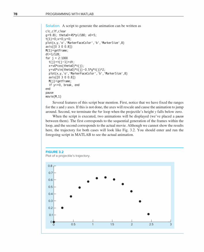
78 ProgrAMMIng wITh MATLAB
Solution. A script to generate the animation can be written asclc,clf,clearg = 9.81; theta0 = 45*pi/180; v0 = 5;t(1) = 0;x = 0;y = 0;plot(x,y,'o','MarkerFaceColor','b','MarkerSize',8)axis([0 3 0 0.8])M(1) = getframe;dt = 1/128;for j = 2:1000 t(j) = t(j − 1) + dt; x = v0*cos(theta0)*t(j); y = v0*sin(theta0)*t(j) − 0.5*g*t(j)^2; plot(x,y,'o','MarkerFaceColor','b','MarkerSize',8) axis([0 3 0 0.8]) M(j) = getframe; if y< = 0, break, endendpausemovie(M,1)
Several features of this script bear mention. First, notice that we have fixed the ranges for the x and y axes. If this is not done, the axes will rescale and cause the animation to jump around. Second, we terminate the for loop when the projectile’s height y falls below zero. When the script is executed, two animations will be displayed (we’ve placed a pause between them). The first corresponds to the sequential generation of the frames within the loop, and the second corresponds to the actual movie. Although we cannot show the results here, the trajectory for both cases will look like Fig. 3.2. You should enter and run the foregoing script in MATLAB to see the actual animation.
FIGURE 3.2Plot of a projectile’s trajectory.
0.8
0.7
0.6
0.5
0.4
0.3
0.2
0.1
00 0.5 1 1.5 2 2.5 3
cha97962_ch03_053-098.indd 78 08/11/16 3:22 pm
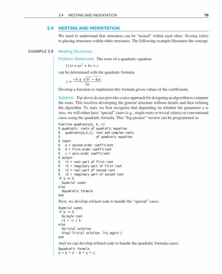
3.4 nESTIng AnD InDEnTATIon 79
3.4 NESTING AND INDENTATION
We need to understand that structures can be “nested” within each other. Nesting refers to placing structures within other structures. The following example illustrates the concept.
EXAMPLE 3.8 nesting Structures
Problem Statement. The roots of a quadratic equationf (x) = ax2 + bx + c
can be determined with the quadratic formula
x = −b ± √_______
b2 − 4ac ______________ 2a
Develop a function to implement this formula given values of the coefficients.
Solution. Top-down design provides a nice approach for designing an algorithm to compute the roots. This involves developing the general structure without details and then refining the algorithm. To start, we first recognize that depending on whether the parameter a is zero, we will either have “special” cases (e.g., single roots or trivial values) or conventional cases using the quadratic formula. This “big-picture” version can be programmed asfunction quadroots(a, b, c)% quadroots: roots of quadratic equation% quadroots(a,b,c): real and complex roots% of quadratic equation% input:% a = second-order coefficient% b = first-order coefficient% c = zero-order coefficient% output:% r1 = real part of first root% i1 = imaginary part of first root% r2 = real part of second root% i2 = imaginary part of second rootif a == 0 %special caseselse %quadratic formulaend
Next, we develop refined code to handle the “special” cases:%special casesif b ~= 0 %single root r1 = −c / belse %trivial solution disp('Trivial solution. Try again')end
And we can develop refined code to handle the quadratic formula cases:%quadratic formulad = b ^ 2 − 4 * a * c;
cha97962_ch03_053-098.indd 79 08/11/16 3:22 pm
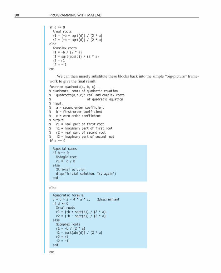
80 ProgrAMMIng wITh MATLAB
if d >= 0 %real roots r1 = (−b + sqrt(d)) / (2 * a) r2 = (−b − sqrt(d)) / (2 * a)else %complex roots r1 = −b / (2 * a) i1 = sqrt(abs(d)) / (2 * a) r2 = r1 i2 = −i1end
We can then merely substitute these blocks back into the simple “big-picture” frame-work to give the final result:function quadroots(a, b, c)% quadroots: roots of quadratic equation% quadroots(a,b,c): real and complex roots% of quadratic equation% input:% a = second-order coefficient% b = first-order coefficient% c = zero-order coefficient% output:% r1 = real part of first root% i1 = imaginary part of first root% r2 = real part of second root% i2 = imaginary part of second rootif a = = 0
%special cases if b ~ = 0 %single root r1 = −c / b else %trivial solution disp('Trivial solution. Try again') end
else
%quadratic formula d = b ^ 2 − 4 * a * c; %discriminant if d >= 0 %real roots r1 = (−b + sqrt(d)) / (2 * a) r2 = (−b − sqrt(d)) / (2 * a) else %complex roots r1 = −b / (2 * a) i1 = sqrt(abs(d)) / (2 * a) r2 = r1 i2 = −i1 end
end
cha97962_ch03_053-098.indd 80 08/11/16 3:22 pm

3.5 PASSIng FUnCTIonS To M-FILES 81
As highlighted by the shading, notice how indentation helps to make the underlying logical structure clear. Also notice how “modular” the structures are. Here is a command window session illustrating how the function performs:>> quadroots(1,1,1)
r1 = −0.5000i1 = 0.8660r2 = −0.5000i2 = −0.8660
>> quadroots(1,5,1)
r1 = −0.2087r2 = −4.7913
>> quadroots(0,5,1)
r1 = −0.2000
>> quadroots(0,0,0)
Trivial solution. Try again
3.5 PASSING FUNCTIONS TO M-FILES
Much of the remainder of the book involves developing functions to numerically eval-uate other functions. Although a customized function could be developed for every new equation we analyzed, a better alternative is to design a generic function and pass the particular equation we wish to analyze as an argument. In the parlance of MATLAB, these functions are given a special name: function functions. Before de-scribing how they work, we will first introduce anonymous functions, which provide a handy means to define simple user-defined functions without developing a full-blown M-file.
3.5.1 Anonymous Functions
Anonymous functions allow you to create a simple function without creating an M-file. They can be defined within the command window with the following syntax:
fhandle = @(arglist) expression
where fhandle = the function handle you can use to invoke the function, arglist = a comma separated list of input arguments to be passed to the function, and expression = any single valid MATLAB expression. For example,
>> f1= @(x,y) x^2 + y^2;
cha97962_ch03_053-098.indd 81 08/11/16 3:22 pm
82 ProgrAMMIng wITh MATLAB
Once these functions are defined in the command window, they can be used just as other functions:
>> f1(3,4)
ans = 25
Aside from the variables in its argument list, an anonymous function can include vari-ables that exist in the workspace where it is created. For example, we could create an anonymous function f(x) = 4x2 as
>> a = 4;>> b = 2;>> f2 = @(x) a*x^b;>> f2(3)
ans = 36
Note that if subsequently we enter new values for a and b, the anonymous function does not change:
>> a = 3;>> f2(3)
ans = 36
Thus, the function handle holds a snapshot of the function at the time it was created. If we want the variables to take on values, we must recreate the function. For example, having changed a to 3,
>> f2 = @(x) a*x^b;
with the result
>> f2(3)
ans = 27
It should be noted that prior to MATLAB 7, inline functions performed the same role as anonymous functions. For example, the anonymous function developed above, f1, could be written as
>> f1 = inline('x^2 + y^2','x','y');
Although they are being phased out in favor of anonymous function, some readers might be using earlier versions, and so we thought it would be helpful to mention them. MATLAB help can be consulted to learn more about their use and limitations.
3.5.2 Function Functions
Function functions are functions that operate on other functions which are passed to it as input arguments. The function that is passed to the function function is referred to as the passed function. A simple example is the built-in function fplot, which plots the graphs of functions. A simple representation of its syntax is
fplot(func,lims)
cha97962_ch03_053-098.indd 82 08/11/16 3:22 pm

3.5 PASSIng FUnCTIonS To M-FILES 83
where func is the function being plotted between the x-axis limits specified by lims = [xmin xmax]. For this case, func is the passed function. This function is “smart” in that it automati-cally analyzes the function and decides how many values to use so that the plot will exhibit all the function’s features.
Here is an example of how fplot can be used to plot the velocity of the free-falling bungee jumper. The function can be created with an anonymous function:
>> vel = @(t) ...sqrt(9.81*68.1/0.25)*tanh(sqrt(9.81*0.25/68.1)*t);
We can then generate a plot from t = 0 to 12 as
>> fplot(vel,[0 12])
The result is displayed in Fig. 3.3.Note that in the remainder of this book, we will have many occasions to use MATLAB’s
built-in function functions. As in the following example, we will also be developing our own.
FIGURE 3.3A plot of velocity versus time generated with the fplot function.
60
50
40
30
20
10
00 2 4 6 8 10 12
cha97962_ch03_053-098.indd 83 08/11/16 3:22 pm

84 ProgrAMMIng wITh MATLAB
EXAMPLE 3.9 Building and Implementing a Function Function
Problem Statement. Develop an M-file function function to determine the average value of a function over a range. Illustrate its use for the bungee jumper velocity over the range from t = 0 to 12 s:
υ (t) = √___
gm ___ cd tanh ( √____
gcd ___ m t )
where g = 9.81, m = 68.1, and cd = 0.25.
Solution. The average value of the function can be computed with standard MATLAB commands as
>> t =linspace(0,12);>> v = sqrt(9.81*68.1/0.25)*tanh(sqrt(9.81*0.25/68.1)*t);>> mean(v)
ans = 36.0870
Inspection of a plot of the function (Fig. 3.3) shows that this result is a reasonable estimate of the curve’s average height. We can write an M-file to perform the same computation:function favg = funcavg(a,b,n)% funcavg: average function height% favg = funcavg(a,b,n): computes average value% of function over a range% input:% a = lower bound of range% b = upper bound of range% n = number of intervals% output:% favg = average value of functionx = linspace(a,b,n);y = func(x);favg = mean(y);end
function f = func(t)f = sqrt(9.81*68.1/0.25)*tanh(sqrt(9.81*0.25/68.1)*t);end
The main function first uses linspace to generate equally spaced x values across the range. These values are then passed to a subfunction func in order to generate the cor-responding y values. Finally, the average value is computed. The function can be run from the command window as>> funcavg (0,12,60)
ans = 36.0127
Now let’s rewrite the M-file so that rather than being specific to func, it evaluates a nonspecific function name f that is passed in as an argument:function favg = funcavg (f,a,b,n)% funcavg: average function height
cha97962_ch03_053-098.indd 84 08/11/16 3:22 pm
3.5 PASSIng FUnCTIonS To M-FILES 85
% favg = funcavg(f,a,b,n): computes average value% of function over a range% input:% f = function to be evaluated% a = lower bound of range% b = upper bound of range% n = number of intervals% output:% favg = average value of functionx = linspace(a,b,n);y = f(x);favg = mean(y);
Because we have removed the subfunction func, this version is truly generic. It can be run from the command window as>> vel = @(t) ...sqrt(9.81*68.1/0.25)*tanh(sqrt(9.81*0.25/68.1)*t);>> funcavg(vel,0,12,60)
ans = 36.0127
To demonstrate its generic nature, funcavg can easily be applied to another case by merely passing it a different function. For example, it could be used to determine the aver-age value of the built-in sin function between 0 and 2π as
>> funcavg(@sin,0,2*pi,180)
ans = −6.3001e − 017
Does this result make sense? We can see that funcavg is now designed to evaluate any valid MATLAB expres-sion. We will do this on numerous occasions throughout the remainder of this text in a number of contexts ranging from nonlinear equation solving to the solution of differential equations.
3.5.3 Passing Parameters
Recall from Chap. 1 that the terms in mathematical models can be divided into depen-dent and independent variables, parameters, and forcing functions. For the bungee jumper model, the velocity (υ) is the dependent variable, time (t) is the independent variable, the mass (m) and drag coefficient (cd) are parameters, and the gravitational constant (g) is the forcing function. It is commonplace to investigate the behavior of such models by perform-ing a sensitivity analysis. This involves observing how the dependent variable changes as the parameters and forcing functions are varied.
In Example 3.9, we developed a function function, funcavg, and used it to determine the average value of the bungee jumper velocity for the case where the parameters were set at m = 68.1 and cd = 0.25. Suppose that we wanted to analyze the same function, but with different parameters. Of course, we could retype the function with new values for each case, but it would be preferable to just change the parameters.
cha97962_ch03_053-098.indd 85 08/11/16 3:22 pm

86 ProgrAMMIng wITh MATLAB
As we learned in Sec. 3.5.1, it is possible to incorporate parameters into anonymous functions. For example, rather than “wiring” the numeric values, we could have done the following:
>> m = 68.1;cd = 0.25;>> vel = @(t) sqrt(9.81*m/cd)*tanh(sqrt(9.81*cd/m)*t);>> funcavg(vel,0,12,60)
ans = 36.0127
However, if we want the parameters to take on new values, we must recreate the anony-mous function.
MATLAB offers a better alternative by adding the term varargin as the function func-tion’s last input argument. In addition, every time the passed function is invoked within the function function, the term varargin{:} should be added to the end of its argument list (note the curly brackets). Here is how both modifications can be implemented for funcavg (omit-ting comments for conciseness):
function favg = funcavg(f,a,b,n,varargin)x = linspace(a,b,n);y = f(x,varargin{:});favg = mean(y);
When the passed function is defined, the actual parameters should be added at the end of the argument list. If we used an anonymous function, this can be done as in
>> vel = @(t,m,cd) sqrt(9.81*m/cd)*tanh(sqrt(9.81*cd/m)*t);
When all these changes have been made, analyzing different parameters becomes easy. To implement the case where m = 68.1 and cd = 0.25, we could enter
>> funcavg(vel,0,12,60,68.1,0.25)
ans = 36.0127
An alternative case, say m = 100 and cd = 0.28, could be rapidly generated by merely changing the arguments:
>> funcavg(vel,0,12,60,100,0.28)
ans = 38.9345
A new Approach for Passing Parameters. At the time of this edition’s develop-ment, MATLAB is going through a transition to a new and better way of passing parameters to function functions. As in the previous example, if the function being passed is
>> vel = @(t,m,cd) sqrt(9.81*m/cd)*tanh(sqrt(9.81*cd/m)*t);
then you invoke the function as
>> funcavg(vel,0,12,60,68.1,0.25)
cha97962_ch03_053-098.indd 86 08/11/16 3:22 pm
3.6 CASE STUDY 87
The Mathworks developers thought this approach was cumbersome, so they devised the following alternative
>> funcavg(@(t) vel(t,68.1,0.25),0,12,60)
Thus, the extra parameters are not strung out at the end making it clear that the parameter list is in the function.
I’ve described both the “old” and the new way of passing parameters because MATLAB will maintain the old way in functions that support in order to minimize backwards incom-patibilities. So if you have old code that has worked in the past, there is no need to go back and convert old code to the new way. For new code, however, I strongly recommend using the new way, because it is easier to read and more versatile.
3.6 CASE STUDY BUngEE JUMPEr VELoCITY
Background. In this section, we will use MATLAB to solve the free-falling bungee jumper problem we posed at the beginning of this chapter. This involves obtaining a solution of
dυ ___ dt = g − cd __ m υ∣υ∣
Recall that, given an initial condition for time and velocity, the problem involved itera-tively solving the formula,
υi+1 = υi + dυi ___ dt Δt
Now also remember that to attain good accuracy, we would employ small steps. Therefore, we would probably want to apply the formula repeatedly to step out from our initial time to attain the value at the final time. Consequently, an algorithm to solve the problem would be based on a loop.
Solution. Suppose that we started the computation at t = 0 and wanted to predict velocity at t = 12 s using a time step of Δt = 0.5 s. We would therefore need to apply the iterative equation 24 times—that is,
n = 12 ___ 0.5 = 24
where n = the number of iterations of the loop. Because this result is exact (i.e., the ratio is an integer), we can use a for loop as the basis for the algorithm. Here’s an M-file to do this including a subfunction defining the differential equation:
function vend = velocity1(dt, ti, tf, vi)% velocity1: Euler solution for bungee velocity% vend = velocity1(dt, ti, tf, vi)% Euler method solution of bungee% jumper velocity% input:% dt = time step (s)% ti = initial time (s)% tf = final time (s)% vi = initial value of dependent variable (m/s)
cha97962_ch03_053-098.indd 87 08/11/16 3:22 pm

88 ProgrAMMIng wITh MATLAB
3.6 CASE STUDY continued
% output:% vend = velocity at tf (m/s) t = ti;v = vi;n = (tf − ti) / dt;for i = 1:n dvdt = deriv(v); v = v + dvdt * dt; t = t + dt;endvend = v;end
function dv = deriv(v)dv = 9.81 − (0.25 / 68.1) * v*abs(v);end
This function can be invoked from the command window with the result:
>> velocity1(0.5,0,12,0)
ans = 50.9259
Note that the true value obtained from the analytical solution is 50.6175 (Exam ple 3.1). We can then try a much smaller value of dt to obtain a more accurate numerical result:
>> velocity1(0.001,0,12,0)
ans = 50.6181
Although this function is certainly simple to program, it is not foolproof. In particu-lar, it will not work if the computation interval is not evenly divisible by the time step. To cover such cases, a while . . . break loop can be substituted in place of the shaded area (note that we have omitted the comments for conciseness):
function vend = velocity2(dt, ti, tf, vi)t = ti;v = vi;h = dt;while(1) if t + dt > tf, h = tf − t; end dvdt = deriv(v); v = v + dvdt * h; t = t + h; if t >= tf, break, endendvend = v;end
function dv = deriv(v)dv = 9.81 − (0.25 / 68.1) * v*abs(v);end
cha97962_ch03_053-098.indd 88 08/11/16 3:22 pm
3.6 CASE STUDY 89
-3.6 CASE STUDY continued
As soon as we enter the while loop, we use a single line if structure to test whether adding t + dt will take us beyond the end of the interval. If not (which would usually be the case at first), we do nothing. If so, we would shorten up the interval—that is, we set the variable step h to the interval remaining: tf – t. By doing this, we guarantee that the last step falls exactly on tf. After we implement this final step, the loop will terminate because the condition t >= tf will test true.
Notice that before entering the loop, we assign the value of the time step dt to another variable h. We create this dummy variable so that our routine does not change the given value of dt if and when we shorten the time step. We do this in anticipation that we might need to use the original value of dt somewhere else in the event that this code were inte-grated within a larger program.
If we run this new version, the result will be the same as for the version based on the for loop structure:
>> velocity2(0.5,0,12,0)
ans = 50.9259
Further, we can use a dt that is not evenly divisible into tf – ti:
>> velocity2(0.35,0,12,0)
ans = 50.8348
We should note that the algorithm is still not foolproof. For example, the user could have mistakenly entered a step size greater than the calculation interval (e.g., tf − ti = 5 and dt = 20). Thus, you might want to include error traps in your code to catch such errors and then allow the user to correct the mistake.
As a final note, we should recognize that the foregoing code is not generic. That is, we have designed it to solve the specific problem of the velocity of the bungee jumper. A more generic version can be developed as
function yend = odesimp(dydt, dt, ti, tf, yi)t = ti; y = yi; h = dt;while (1) if t + dt > tf, h = tf − t; end y = y + dydt(y) * h; t = t + h; if t >= tf, break, endendyend = y;
Notice how we have stripped out the parts of the algorithm that were specific to the bungee example (including the subfunction defining the differential equation) while keep-ing the essential features of the solution technique. We can then use this routine to solve
cha97962_ch03_053-098.indd 89 08/11/16 3:22 pm
90 ProgrAMMIng wITh MATLAB
3.6 CASE STUDY continued
the bungee jumper example, by specifying the differential equation with an anonymous function and passing its function handle to odesimp to generate the solution
>> dvdt=@(v) 9.81−(0.25/68.1)*v*abs(v);>> odesimp(dvdt,0.5,0,12,0)
ans = 50.9259
We could then analyze a different function without having to go in and modify the M-file. For example, if y = 10 at t = 0, the differential equation dy∕dt = −0.1y has the analytical solution y = 10e−0.1t. Therefore, the solution at t = 5 would be y(5) = 10e−0.1(5) = 6.0653. We can use odesimp to obtain the same result numerically as in
>> odesimp(@(y) −0.1*y,0.005,0,5,10)
ans = 6.0645
Finally, we can use varargin and the new way of passing parameters to develop a final and superior version. To do this, the odesimp function is first modified by adding the high-lighted code
function yend = odesimp2(dydt, dt, ti, tf, yi, varargin)t = ti; y = yi; h = dt;while (1) if t + dt > tf, h = tf − t; end y = y + dydt(y, varargin{:}) * h; t = t + h; if t >= tf, break, endendyend = y;
Then, we can develop a script to perform the computation,
clcformat compactdvdt=@(v,cd,m) 9.81−(cd/m)*v*abs(v);odesimp2(@(v) dvdt(v,0.25,68.1),0.5,0,12,0)
which yields the correct result
ans = 50.9259
cha97962_ch03_053-098.indd 90 08/11/16 3:22 pm

ProBLEMS 91
PROBLEMS
3.1 Figure P3.1 shows a cylindrical tank with a conical base. If the liquid level is quite low, in the conical part, the volume is simply the conical volume of liquid. If the liquid level is midrange in the cylindrical part, the total volume of liquid includes the filled conical part and the partially filled cylindrical part.
Use decisional structures to write an M-file to compute the tank’s volume as a function of given values of R and d. Design the function so that it returns the volume for all cases
2R
R
d
FIGURE P3.1
where the depth is less than 3R. Return an error message (“Overtop”) if you overtop the tank—that is, d > 3R. Test it with the following data:
R 0.9 1.5 1.3 1.3d 1 1.25 3.8 4.0
Note that the tank’s radius is R.3.2 An amount of money P is invested in an account where interest is compounded at the end of the period. The future worth F yielded at an interest rate i after n periods may be determined from the following formula:
F = P(1 + i)n
Write an M-file that will calculate the future worth of an investment for each year from 1 through n. The input to the function should include the initial investment P, the interest rate i (as a decimal), and the number of years n for which the future worth is to be calculated. The output should consist of a table with headings and columns for n and F. Run the program for P = $100,000, i = 0.05, and n = 10 years.3.3 Economic formulas are available to compute annual payments for loans. Suppose that you borrow an amount of money P and agree to repay it in n annual payments at
an interest rate of i. The formula to compute the annual payment A is
A = P i (1 + i )n ___________ (1 + i )n − 1
Write an M-file to compute A. Test it with P = $100,000 and an interest rate of 3.3% (i = 0.033). Compute results for n = 1, 2, 3, 4, and 5 and display the results as a table with head-ings and columns for n and A.3.4 The average daily temperature for an area can be ap-proximated by the following function:
T = Tmean + (Tpeak − Tmean) cos(ω(t − tpeak))
where Tmean = the average annual temperature, Tpeak = the peak temperature, ω = the frequency of the annual varia-tion (= 2π/365), and tpeak = day of the peak temperature (≅205 d). Parameters for some U.S. towns are listed here:
City Tmean (°C) Tpeak (°C)
Miami, FL 22.1 28.3Yuma, AZ 23.1 33.6Bismarck, ND 5.2 22.1Seattle, WA 10.6 17.6Boston, MA 10.7 22.9
Develop an M-file that computes the average temperature between two days of the year for a particular city. Test it for (a) January–February in Yuma, AZ (t = 0 to 59) and (b) July–August temperature in Seattle, WA (t = 180 to 242).3.5 The sine function can be evaluated by the following infinite series:
sin x = x − x3 __ 3! + x
5 __ 5! − · · ·
Create an M-file to implement this formula so that it com-putes and displays the values of sin x as each term in the series is added. In other words, compute and display in sequence the values for
sin x = x
sin x = x − x3 __ 3!
sin x = x − x3 __ 3! + x
5 __ 5!
...
cha97962_ch03_053-098.indd 91 08/11/16 3:22 pm
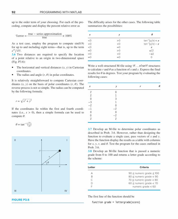
92 ProgrAMMIng wITh MATLAB
up to the order term of your choosing. For each of the pre-ceding, compute and display the percent relative error as
%error = true − series approximation _______________________ true × 100%
As a test case, employ the program to compute sin(0.9) for up to and including eight terms—that is, up to the term x15∕15!.3.6 Two distances are required to specify the location of a point relative to an origin in two-dimensional space (Fig. P3.6):
• The horizontal and vertical distances (x, y) in Cartesian coordinates.
• The radius and angle (r, θ ) in polar coordinates.
It is relatively straightforward to compute Cartesian coor-dinates (x, y) on the basis of polar coordinates (r, θ ). The reverse process is not so simple. The radius can be computed by the following formula:
r = √______
x2 + y2
If the coordinates lie within the first and fourth coordi-nates (i.e., x > 0), then a simple formula can be used to compute θ:
θ = tan−1 ( y __ x )
The difficulty arises for the other cases. The following table summarizes the possibilities:
x y θ
<0 >0 tan−1( y∕x) + π<0 <0 tan−1(y∕x) − π<0 =0 π=0 >0 π∕2=0 <0 −π2=0 =0 0
Write a well-structured M-file using if...elseif structures to calculate r and θ as a function of x and y. Express the final results for θ in degrees. Test your program by evaluating the following cases:
x y r θ
2 02 10 3
−3 1−2 0−1 −20 00 −22 2
3.7 Develop an M-file to determine polar coordinates as described in Prob. 3.6. However, rather than designing the function to evaluate a single case, pass vectors of x and y. Have the function display the results as a table with columns for x, y, r, and θ. Test the program for the cases outlined in Prob. 3.6.3.8 Develop an M-file function that is passed a numeric grade from 0 to 100 and returns a letter grade according to the scheme:
Letter Criteria
A 90 ≤ numeric grade ≤ 100B 80 ≤ numeric grade < 90C 70 ≤ numeric grade < 80D 60 ≤ numeric grade < 70F numeric grade < 60
The first line of the function should be
function grade = lettergrade(score)FIGURE P3.6
y
xθ
III
III IV
r
cha97962_ch03_053-098.indd 92 08/11/16 3:22 pm

ProBLEMS 93
Design the function so that it displays an error message and terminates in the event that the user enters a value of score that is less than zero or greater than 100. Test your function with 89.9999, 90, 45, and 120.3.9 Manning’s equation can be used to compute the velocity of water in a rectangular open channel:
U = √__
S ____ n ( BH _______ B + 2H ) 2∕3
where U = velocity (m/s), S = channel slope, n = roughness coefficient, B = width (m), and H = depth (m). The follow-ing data are available for five channels:
n S B H
0.036 0.0001 10 20.020 0.0002 8 10.015 0.0012 20 1.50.030 0.0007 25 30.022 0.0003 15 2.6
Write an M-file that computes the velocity for each of these channels. Enter these values into a matrix where each column represents a parameter and each row represents a channel. Have the M-file display the input data along with the computed velocity in tabular form where velocity is the fifth column. Include headings on the table to label the columns.3.10 A simply supported beam is loaded as shown in Fig. P3.10. Using singularity functions, the displacement along the beam can be expressed by the equation:
uy(x) = −5 ___ 6 [⟨x − 0⟩4 − ⟨x − 5⟩4] + 15 ___ 6 ⟨x − 8⟩3
+ 75 ⟨x − 7⟩2 + 57 ___ 6 x3 − 238.25x
By definition, the singularity function can be expressed as follows:
⟨x − a⟩n = { (x − a)n when x > a } 0 when x ≤ a
Develop an M-file that creates a plot of displacement (dashed line) versus distance along the beam, x. Note that x = 0 at the left end of the beam.3.11 The volume V of liquid in a hollow horizontal cylinder of radius r and length L is related to the depth of the liquid h by
V = [ r2 cos–1 ( r – h ____ r ) − (r − h) √_______
2rh − h2 ] LDevelop an M-file to create a plot of volume versus depth. Here are the first few lines:
function cylinder(r, L, plot_title)% volume of horizontal cylinder% inputs:% r = radius% L = length% plot_title = string holding plot title
Test your program with
>> cylinder(3,5,...'Volume versus depth for horizontal... cylindrical tank')
3.12 Develop a vectorized version of the following code:
tstart = 0; tend = 20; ni = 8;t(1) = tstart;y(1) = 12 + 6*cos(2*pi*t(1)/(tend−tstart));for i = 2:ni+1 t(i) = t(i–1)+(tend-tstart)/ni; y(i) = 12 + 6*cos(2*pi*t(i)/ ...
(tend–tstart));end
20 kips/ft
150 kip-ft15 kips
5ʹ 2ʹ 1ʹ 2ʹ
FIGURE P3.10
cha97962_ch03_053-098.indd 93 08/11/16 3:22 pm
94 ProgrAMMIng wITh MATLAB
3.13 The “divide and average” method, an old-time method for approximating the square root of any positive number a, can be formulated as
x = x + a∕x _______ 2
Write a well-structured M-file function based on the while...break loop structure to implement this algorithm. Use proper indentation so that the structure is clear. At each step estimate the error in your approximation as
ε = | xnew − xold _________ xnew |
Repeat the loop until ε is less than or equal to a specified value. Design your program so that it returns both the re-sult and the error. Make sure that it can evaluate the square root of numbers that are equal to and less than zero. For the latter case, display the result as an imaginary number. For example, the square root of −4 would return 2i. Test your program by evaluating a = 0, 2, 10 and −4 for ε = 1 × 10⁻⁴. 3.14 Piecewise functions are sometimes useful when the re-lationship between a dependent and an independent variable cannot be adequately represented by a single equation. For example, the velocity of a rocket might be described by
10t2 − 5t 0 ≤ t ≤ 8 624 − 3t 8 ≤ t ≤ 16
υ(t) = { 36t + 12(t − 16)2 16 ≤ t ≤ 26 2136e−0.1(t−26) t > 26
0 otherwise
Develop an M-file function to compute υ as a function of t. Then, develop a script that uses this function to generate a plot of υ versus t for t = −5 to 50.3.15 Develop an M-file function called rounder to round a number x to a specified number of decimal digits, n. The first line of the function should be set up as
function xr = rounder(x, n)
Test the program by rounding each of the following to 2 dec-imal digits: x = 477.9587, −477.9587, 0.125, 0.135, −0.125, and −0.135. 3.16 Develop an M-file function to determine the elapsed days in a year. The first line of the function should be set up as
function nd = days(mo, da, leap)
where mo = the month (1–12), da = the day (1–31), and leap = (0 for non–leap year and 1 for leap year). Test it for January 1, 1997, February 29, 2004, March 1, 2001, June 21, 2004,
and December 31, 2008. Hint: A nice way to do this com-bines the for and the switch structures.3.17 Develop an M-file function to determine the elapsed days in a year. The first line of the function should be set up as
function nd = days(mo, da, year)
where mo = the month (1–12), da = the day (1–31), and year = the year. Test it for January 1, 1997, February 29, 2004, March 1, 2001, June 21, 2004, and December 31, 2008.3.18 Develop a function function M-file that returns the difference between the passed function’s maximum and minimum value given a range of the independent variable. In addition, have the function generate a plot of the function for the range. Test it for the following cases:(a) f(t) = 8e−0.25tsin(t − 2) from t = 0 to 6π.(b) f(x) = e4xsin(1∕x) from x = 0.01 to 0.2.(c) The built-in humps function from x = 0 to 2.3.19 Modify the function function odesimp developed at the end of Sec. 3.6 so that it can be passed the arguments of the passed function. Test it for the following case:
>> dvdt = @(v,m,cd) 9.81−(cd/m)*v^2;>> odesimp(dvdt,0.5,0,12,−10,70,0.23)
3.20 A Cartesian vector can be thought of as representing magnitudes along the x-, y-, and z-axes multiplied by a unit vector (i, j, k). For such cases, the dot product of two of these vectors {a} and {b} corresponds to the product of their mag-nitudes and the cosine of the angle between their tails as in
{a}·{b} = ab cosθ
The cross product yields another vector, {c} = {a} × {b}, which is perpendicular to the plane defined by {a} and {b} such that its direction is specified by the right-hand rule. Develop an M-file function that is passed two such vectors and returns θ, {c} and the magnitude of {c}, and generates a three-dimensional plot of the three vectors {a}, {b}, and {c) with their origins at zero. Use dashed lines for {a} and {b} and a solid line for {c}. Test your function for the fol-lowing cases:
(a) a = [6 4 2]; b = [2 6 4]; (b) a = [3 2 −6]; b = [4 −3 1];(c) a = [2 −2 1]; b = [4 2 −4];(d) a = [−1 0 0]; b = [0 −1 0];
3.21 Based on Example 3.7, develop a script to produce an animation of a bouncing ball where υ0 = 5 m/s and θ0 = 50°. To do this, you must be able to predict exactly when the ball hits the ground. At this point, the direction changes (the new angle will equal the negative of the angle at impact), and the
cha97962_ch03_053-098.indd 94 08/11/16 3:22 pm

ProBLEMS 95
% precomputationsd = 2 * r; Ta = TC + 273.15; Ab = pi / 4 * d ^ 2;Vb = pi / 6 * d ^ 3; rhog = P / Rgas / Ta; mG = Vb * rhog;FB = Vb * rhoa * g; FG = mG * g; cdp = rhoa * Ab * CD / 2;
% compute times, velocities and elevations[t,y] = Balloon(FB, FG, mG, cdp, mP, md, zd, ti,vi,zi,tf,dt);
% Display resultsYour code to display a nice labeled table of times, velocities, and elevations
% Plot resultsYour code to create a nice labeled plot of velocity and elevation versus time.
Your function should be structured like:
function [tout,yout]=Balloon(FB, FG, mG, cdp, mP, md, zd, ti,vi,zi,tf,dt)global g
% balloon% function [tout,yout]=Balloon(FB, FG, mG, cdp, mP1, md, zd, ti,vi,zi,tf,dt)% Function to generate solutions of vertical velocity and elevation % versus time with Euler’s method for a hot air balloon% Input:% FB = buoyancy force (N)% FG = gravity force (N)% mG = mass (kg)% cdp=dimensional drag coefficient% mP= mass of payload (kg)% md=mass jettisoned (kg)% zd=elevation at which mass is jettisoned (m)% ti = initial time (s)% vi=initial velocity (m/s)% zi=initial elevation (m)% tf = final time (s)% dt=integration time step (s)% Output:% tout = vector of times (s)% yout[:,1] = velocities (m/s)% yout[:,2] = elevations (m)% Code to implement Euler’s method to compute output and plot results
3.25 A general equation for a sinusoid can be written as
y(t) = _ y + Δy sin (2πft − ϕ)
velocity will decrease in magnitude to reflect energy loss due to the collision of the ball with the ground. The change in velocity can be quantified by the coefficient of restitution CR which is equal to the ratio of the velocity after to the velocity before impact. For the present case, use a value of CR = 0.8.3.22 Develop a function to produce an animation of a par-ticle moving in a circle in Cartesian coordinates based on radial coordinates. Assume a constant radius, r, and allow the angle, θ, to increase from zero to 2π in equal increments. The function’s first lines should be
function phasor(r, nt, nm)% function to show the orbit of a phasor% r = radius% nt = number of increments for theta% nm = number of movies
Test your function with
phasor(1, 256, 10)
3.23 Develop a script to produce a movie for the butterfly plot from Prob. 2.22. Use a particle located at the x-y coordi-nates to visualize how the plot evolves in time.3.24 Develop a MATLAB script to compute the velocity, υ, and position, z, of a hot air balloon as described in Prob. 1.28. Perform the calculation from t = 0 to 60 s with a step size of 1.6 s. At z = 200 m, assume that part of the payload (100 kg) is dropped out of the balloon. Your script should be struc-tured like:
% YourFullName% Hot Air Balloon Script
clear,clc,clf
g = 9.81;global g
% set parametersr = 8.65; % balloon radiusCD = 0.47; % dimensionless drag coefficientmP = 265; % mass of payloadP = 101300; % atmospheric pressureRgas = 287; % Universal gas constant for dry airTC = 100; % air temperaturerhoa = 1.2; % air densityzd = 200; % elevation at which mass is jettisonedmd = 100; % mass jettisonedti = 0; % initial time (s)tf = 60; % final time (s)vi = 0; % initial velocityzi = 0; % initial elevationdt = 1.6; % integration time step
cha97962_ch03_053-098.indd 95 08/11/16 3:22 pm
96 ProgrAMMIng wITh MATLAB
Step 7: Compute new values for m = m/2 and n = (300 + n)/2, and then go to Step 9.
Step 8: Compute new values for m = (300 + m)/2 and n = (300 + n)/2.
Step 9: If i is less than 1000 then go to Step 10. Otherwise, go to Step 11.
Step 10: Plot a point at the coordinate,(m,n).Step 11: Terminate ii loop.Step 12: Set hold off.
Develop a MATLAB script for this algorithm using for and if structures. Run it for the following two cases (a) m = 2 and n = 1 and (b) m = 100 and n = 200.3.27 Write a well-structured MATLAB function procedure named Fnorm to calculate the Frobenius norm of an m×n matrix,
∥A∥f = √_________
∑ i=1
m
∑ j=1
n
a i,j 2
Here is a script that uses the functionA = [5 7 9; 1 8 4; 7 6 2];Fn = Fnorm(A)
Here is the first line of the functionfunction Norm = Fnorm(x)
Develop two versions of the function: (a) using nested for loops and (b) using sum functions.3.28 The pressure and temperature of the atmosphere are constantly changing depending on a number of factors in-cluding altitude, latitude/longitude, time of day, and season. To take all these variations into account when considering the design and performance of flight vehicles is impracti-cal. Therefore, a standard atmosphere is frequently used to provide engineers and scientists with a common reference for their research and development. The International Stan-dard Atmosphere is one such model of how conditions of the earth’s atmosphere change over a wide range of altitudes or elevations. The following table shows values of temperature and pressure at selected altitudes.
where y = the dependent variable, _ y = the mean value, Δy =
the amplitude, f = the ordinary frequency (i.e., the number of oscillations that occur each unit of time), t = the independent variable (in this case time), and ϕ = phase shift. Develop a MATLAB script to generate a 5 panel vertical plot to il-lustrate how the function changes as the parameters change. On each plot display the simple sine wave, y(t) = sin(2πt), as a red line. Then, add the following functions to each of the 5 panels as black lines:
subplot Function Title
5,1,1 y(t) = 1 + sin(2πt) (a) Effect of mean5,1,2 y(t) = 2sin(2πt) (b) Effect of amplitude 5,1,3 y(t) = sin(4πt) (c) Effect of frequency 5,1,4 y(t) = sin(2πt − π/4) (d) Effect of phase shift5,1,5 y(t) = cos(2πt −π/2) (e) Relationship of sine to cosine
Employ a range of t = 0 to 2π and scale each subplot so that the abscissa goes from 0 to 2π and the ordinate goes from −2 to 2. Include the titles with each subplot, label each subplot’s ordinate as 'f(t)', and the bottom plot’s abscissa as 't'. 3.26 A fractal is a curve or geometric figure, each part of which has the same statistical character as the whole. Fractals are useful in modeling structures (such as eroded coastlines or snowflakes) in which similar patterns recur at progressively smaller scales, and in describing partly random or chaotic phenomena such as crystal growth, fluid turbulence, and gal-axy formation. Devaney (1990) has written a nice little book that includes a simple algorithm to create an interesting fractal pattern. Here is a step-by-step description of this algorithm:
Step 1: Assign value to m and n and set hold on.Step 2: Start a for loop to iterate over ii = 1:100000 Step 3: Compute a random number, q = 3*rand(1)Step 4: If the value of q is less than 1 go to Step 5. Otherwise
go to Step 6.Step 5: Compute new values for m = m/2 and n = n/2 and
then go to Step 9.Step 6: If the value of q is less than 2 go to Step 7. Otherwise
go to Step 8.
Layer Index, i
Layer Name
Base Geopotential Altitude Above MSL, h (km)
Lapse Rate (ºC/km)
Base Temperature T (ºC)
Base Pressure, p (Pa)
1 Troposphere 0 −6.5 15 101,3252 Tropopause 11 0 −56.5 22,6323 Stratosphere 20 1 −56.5 5474.94 Stratosphere 32 2.8 −44.5 868.025 Stratopause 47 0 −2.5 110.916 Mesosphere 51 −2.8 −2.5 66.9397 Mesosphere 71 −2.0 −58.5 3.95648 Mesopause 84.852 — −86.28 0.3734
cha97962_ch03_053-098.indd 96 08/11/16 3:22 pm
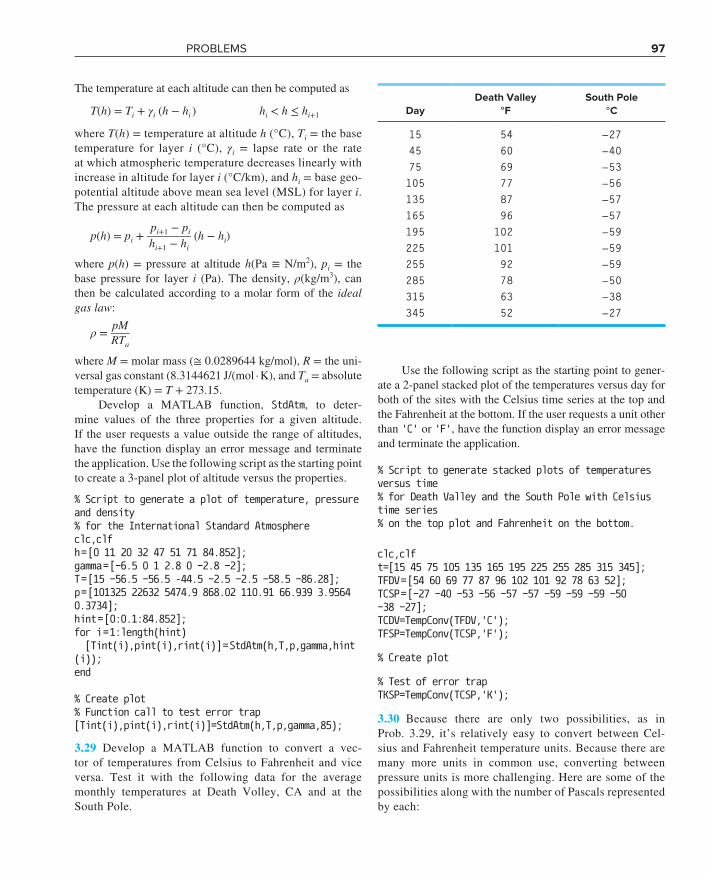
ProBLEMS 97
The temperature at each altitude can then be computed as
T(h) = Ti + γi (h − hi ) hi < h ≤ hi+1
where T(h) = temperature at altitude h (°C), Ti = the base temperature for layer i (°C), γi = lapse rate or the rate at which atmospheric temperature decreases linearly with increase in altitude for layer i (°C/km), and hi = base geo-potential altitude above mean sea level (MSL) for layer i. The pressure at each altitude can then be computed as
p(h) = pi + pi+1 − pi ________ hi+1 − hi
(h − hi)
where p(h) = pressure at altitude h(Pa ≡ N/m2), pi = the base pressure for layer i (Pa). The density, ρ(kg/m3), can then be calculated according to a molar form of the ideal gas law:
ρ = pM ____ RTa
where M = molar mass (≅ 0.0289644 kg/mol), R = the uni-versal gas constant (8.3144621 J/(mol · K), and Ta = absolute temperature (K) = T + 273.15.
Develop a MATLAB function, StdAtm, to deter-mine values of the three properties for a given altitude. If the user requests a value outside the range of altitudes, have the function display an error message and terminate the application. Use the following script as the starting point to create a 3-panel plot of altitude versus the properties.
% Script to generate a plot of temperature, pressure and density% for the International Standard Atmosphereclc,clfh = [0 11 20 32 47 51 71 84.852];gamma = [−6.5 0 1 2.8 0 −2.8 −2];T = [15 −56.5 −56.5 -44.5 −2.5 −2.5 −58.5 −86.28];p = [101325 22632 5474.9 868.02 110.91 66.939 3.9564 0.3734];hint = [0:0.1:84.852];for i = 1:length(hint) [Tint(i),pint(i),rint(i)] = StdAtm(h,T,p,gamma,hint(i));end
% Create plot% Function call to test error trap[Tint(i),pint(i),rint(i)]=StdAtm(h,T,p,gamma,85);
3.29 Develop a MATLAB function to convert a vec-tor of temperatures from Celsius to Fahrenheit and vice versa. Test it with the following data for the average monthly temperatures at Death Volley, CA and at the South Pole.
Use the following script as the starting point to gener-ate a 2-panel stacked plot of the temperatures versus day for both of the sites with the Celsius time series at the top and the Fahrenheit at the bottom. If the user requests a unit other than 'C' or 'F', have the function display an error message and terminate the application.
% Script to generate stacked plots of temperatures versus time% for Death Valley and the South Pole with Celsius time series% on the top plot and Fahrenheit on the bottom.
clc,clft=[15 45 75 105 135 165 195 225 255 285 315 345]; TFDV = [54 60 69 77 87 96 102 101 92 78 63 52];TCSP = [−27 −40 −53 −56 −57 −57 −59 −59 −59 −50 −38 −27];TCDV=TempConv(TFDV,'C');TFSP=TempConv(TCSP,'F');
% Create plot
% Test of error trapTKSP=TempConv(TCSP,'K');
3.30 Because there are only two possibilities, as in Prob. 3.29, it’s relatively easy to convert between Cel-sius and Fahrenheit temperature units. Because there are many more units in common use, converting between pressure units is more challenging. Here are some of the possibilities along with the number of Pascals represented by each:
Day
Death Valley °F
South Pole °C
15 54 −2745 60 −4075 69 −53105 77 −56135 87 −57165 96 −57195 102 −59225 101 −59255 92 −59285 78 −50315 63 −38345 52 −27
cha97962_ch03_053-098.indd 97 08/11/16 3:22 pm
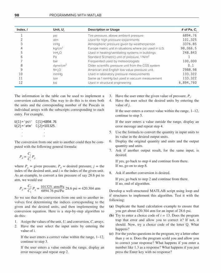
98 ProgrAMMIng wITh MATLAB
3. Have the user enter the given value of pressure, Pi.4. Have the user select the desired units by entering the
value of j.If the user enters a correct value within the range, 1–12, continue to step 5.
If the user enters a value outside the range, display an error message and repeat step 4.
5. Use the formula to convert the quantity in input units to its value in the desired output units.
6. Display the original quantity and units and the output quantity and units.
7. Ask if another output result, for the same input, is desired.
If yes, go back to step 4 and continue from there.If no, go on to step 8.
8. Ask if another conversion is desired.
If yes, go back to step 2 and continue from there.If no, end of algorithm.
Develop a well-structured MATLAB script using loop and if structures to implement this algorithm. Test it with the following:
(a) Duplicate the hand calculation example to ensure that you get about 420.304 atm for an input of 28.6 psi.
(b) Try to enter a choice code of i = 13. Does the program trap that error and allow you to correct it? If not, it should. Now, try a choice code of the letter Q. What happens?
(c) For the yes/no questions in the program, try a letter other than y or n. Does the program scold you and allow you to correct your response? What happens if you enter a number like 1.3 as a response? What happens if you just press the Enter key with no response?
The information in the table can be used to implement a conversion calculation. One way to do this is to store both the units and the corresponding number of the Pascals in individual arrays with the subscripts corresponding to each entry. For example,
U(1) = 'psi' C(1)=6894.76U(2) = 'atm' C(2)=101325. · · · · · ·
The conversion from one unit to another could then be com-puted with the following general formula:
Pd = Cj __ Ci
Pg
where Pg = given pressure, Pd = desired pressure, j = the index of the desired unit, and i = the index of the given unit. As an example, to convert a tire pressure of say 28.6 psi to atm, we would use
Pd = C2 ___ C1
Pg = 101325. atm /Pa _____________ 6894.76 psi /Pa 28.6 psi = 420.304 atm
So we see that the conversion from one unit to another in-volves first determining the indices corresponding to the given and the desired units, and then implementing the conversion equation. Here is a step-by-step algorithm to do this:1. Assign the values of the unit, U, and conversion, C, arrays.2. Have the user select the input units by entering the
value of i.
If the user enters a correct value within the range, 1–12, continue to step 3.If the user enters a value outside the range, display an error message and repeat step 2.
Index, i Unit, Ui Description or Usage # of Pa, Ci
1 psi Tire pressure, above ambient pressure 6894.762 atm Used for high pressure experiments 101,3253 inHg Atmospheric pressure given by weatherperson 3376.854 kg/cm2 Europe metric unit in situations where psi used in U.S. 98,066.55 inH2O Used in heating/ventilating systems in buildings 248.8436 Pa Standard SI (metric) unit of pressure, 1 N/m2 17 bar Frequented used by meteorologists 100,0008 dyne/cm2 Older scientific pressure unit from the CGS system 0.19 ftH2O American and English low value pressure unit. 2988.9810 mmHg Used in laboratory pressure measurements 133.32211 torr Same as 1 mmHg but used in vacuum measurement 133.32212 ksi Used in structural engineering 6,894,760
cha97962_ch03_053-098.indd 98 08/11/16 3:22 pm