APPROVED: Shengli Fu, Major Professor Murali Varanasi, Committee Member Kamesh Namuduri, Committee Member Shengli Fu, Graduate Program

Coordinator Murali Varanasi, Chair of the

Department of Electrical Engineering

Costas Tsatsoulis, Dean of the College of Engineering

James D. Meernik, Acting Dean of the Toulouse Graduate School

MATLAB IMPLEMENTATION OF A TORNADO FORWARD

ERROR CORRECTION CODE

Alexandra Noriega

Thesis Prepared for the Degree of

MASTER OF SCIENCE

UNIVERSITY OF NORTH TEXAS

May 2011

Noriega, Alexandra. Matlab Implementation of a Tornado Forward Error

Correction Code. Master of Science (Electrical Engineering), May 2011, 53 pp., 12

figures, bibliography, 16 titles.

This research discusses how the design of a tornado forward error correcting

channel code (FEC) sends digital data stream profiles to the receiver. The complete

design was based on the Tornado channel code, binary phase shift keying (BPSK)

modulation on a Gaussian channel (AWGN). The communication link was simulated by

using Matlab, which shows the theoretical systems efficiency. Then the data stream was

input as data to be simulated communication systems using Matlab. The purpose of this

paper is to introduce the audience to a simulation technique that has been successfully

used to determine how well a FEC expected to work when transferring digital data

streams. The goal is to use this data to show how FEC optimizes a digital data stream

to gain a better digital communications systems. The results conclude by making

comparisons of different possible styles for the Tornado FEC code.

ii

Copyright 2011

by

Alexandra Noriega

iii

ACKNOWLEDGEMENTS

I would like to thank Dr. Fu for his guidance in my thesis and in my master's

course work. I will also like to thank Dr. Varanasi and Dr. Namaduri for participating as

my defense committee.

A special thanks to my son Gianni Noriega, who has been my biggest inspiration

since he was born and my fiancé, Juan Carlos Franco, who has always been there

throughout my master's career and thesis. I want to thank my family for been supportive

and understanding of my goals.

iv

TABLE OF CONTENTS

Page ACKNOWLEDGEMENTS ............................................................................................... iii LIST OF FIGURES .......................................................................................................... vi Chapters

1. INTRODUCTION ....................................................................................... 1 2. GRAPH THEORY ...................................................................................... 6

2.1 Introduction ..................................................................................... 6 2.2 Defintion of Graphs ......................................................................... 6

2.2.1 Regular Graph ...................................................................... 8 2.2.2 Irregular Graph ..................................................................... 9

2.3 Construction of Irregular Graphs ................................................... 10 2.4 Conclusion .................................................................................... 12

3. LOW DENSITY PARITY CHECK ............................................................. 13

3.1 Definition of LDPC and Its Properties ............................................ 13 3.1.1 Definition of LDPC .............................................................. 13

3.2 Preparation of the Encoder ........................................................... 14 3.3 Preparation of the Decoder ........................................................... 15 3.4 Conclusion .................................................................................... 20

4. REED SOLOMON ................................................................................... 21

4.1 Introduction ................................................................................... 21 4.2 Definition of Reed Solomon and Its Properties ............................. 22 4.3 Preparation of the Encoder ........................................................... 23 4.4 Preparation of the Decoder ........................................................... 23 4.5 Conclusion .................................................................................... 25

5. FOUNTAIN CODES ................................................................................. 26

5.1 Introduction ................................................................................... 26 5.2 Definition of Reed Solomon and its Properties .............................. 26 5.3 Preparation of the Encoder ........................................................... 28

v

5.4 Preparation of the Decoder ........................................................... 28 5.5 Degree Sequences of Irregular Graph .......................................... 29 5.6 Conclusion .................................................................................... 30

6. TORNADO CODE ................................................................................... 31

6.1 Introduction ................................................................................... 31 6.1.1 Terminology ........................................................................ 32 6.1.2 Description of Codes .......................................................... 32 6.1.3 Encoding Rate .................................................................... 32 6.1.4 Decoding ............................................................................ 34

6.2 Introduction of BPSK Modulation .................................................. 35 6.3 BPSK System Model ..................................................................... 36 6.4 Tornado Code Construction .......................................................... 37

7. CONCLUSION AND FUTURE WORK ..................................................... 40

Appendices

A. IRREGULAR MATRIX GENERATOR ...................................................... 41 B. TORNADO CODE ................................................................................... 48

BIBLIOGRAPHY ........................................................................................................... 50

vi

LIST OF FIGURES

Page 1.1 Digital communications blocks .............................................................................. 4

2.1 Irregular tree ....................................................................................................... 11

3.1 LDPC encoder flowchart ..................................................................................... 15

4.1 Linear codes family tree ..................................................................................... 22

6.1 Encoder and decoder cascade ........................................................................... 33

6.2 Encoder and decoder cascade using XOR ......................................................... 34

6.3 Bipartite graph decoding ..................................................................................... 35

6.4 Two bits been mapped using BPSK modulation ................................................. 37

6.5 512x1024 irregular matrix ................................................................................... 37

6.6 256x512 irregular matrix ..................................................................................... 38

6.7 128x256 irregular matrix ..................................................................................... 38

6.8 BER vs. SNR ...................................................................................................... 39

CHAPTER 1

INTRODUCTION

The topic of this paper is investigating a forward error correction scheme in the �eld of

coding theory, speci�cally using a form of fountain code called Tornado code which is classi�ed

as a systematic block code [24]. The concept of the forward error correction scheme is found

in Chapter 1. The Tornado code o�ers a quick and e�cient encoding and decoding algorithm

speeds. The focus is on an algorithm of the Tornado systematic block code using an erasure

channel and a Gaussian channel. Matlab is also utilized to show a way to provide reliable

transmission of the algorithm for the Tornado code.

The speci�c reasons why I chose to focus on Tornado forward error correction code was

due to interest in digital communications, which grew immensely at Los Alamos National

Laboratory, where I interned in the summer of 2009 in the Space Program division. Another

internship at Northrop Grumman during the summer of 2010 provided an opportunity to look

into fountain codes. Also, fountain codes such as the Tornado code, is a root of the Digital

Fountain company, which is a record-breaking sparse-graph codes for channels with erasures.

Another reason for this research is because of the demand for e�cient and reliable digital

data transmission and storage systems. Thus, Tornado code was chosen because it is the

precursor to the current fountain codes which have very e�cient linear time encoding and

decoding algorithms and it requires small constant values of XOR operations per generated

system for both the encoder and the decoder[24].

The thesis background information on the communications topic began with Claude Shan-

non, the father of information theory. In 1937, Shannon de�ned channel capacity, which states

that for a limited rate of information, one can achieve a small error probability. The small

1

error probability is caused by unbeatable noise. Channel capacity de�nes the upper bound for

digital transmission to be able to receive reliable data[7].

Forward error correction, also known as channel coding, is a control system to correct

errors created in a corrupted channel by noise. An error correcting code therefore detects

and corrects erroneous transmitted data up to a proximity of reaching a channel capacity. All

type of correcting and detecting codes attempt to achieve for Shannon's channel capacity.

Shannon de�ned channel capacity, but Richard Hamming was the �rst pioneer to design the

�rst error correcting code. An error correcting code averages the noise and adds redundancy

to its messages, thus adding reliability. Therefore, if a bit ipped due to noise, the receiver can

detect and correct a limited amount of errors from its neighbouring bits, costing the system a

larger bandwidth. For the most part error correcting codes are used for large storage devices.

The amount of errors that are able to be detected and corrected are set by the type of forward

error correction code[7].

There are two main types of codes in channel coding are used in forward error correction.

These are block codes and convolutional codes. The encoder splits the information string

into message blocks of k information bits each. A message is shown as a binary block

k � tuple u = (u1; u2; :::; uk) where in a block code, the symbol u is used to refer a k-bit

message instead of the full information succession. The total number of possible messages

are 2k. The codeword at the encoder converts each message u into discrete symbols of

n� tuple = (v1; v2; :::; vk) were in block coding, the symbol v is used to refer to an n-symbol

block instead of the full encoded succession. Similar to the total amount of messages, there

are 2k combination of possible codewords at the output of the encoder. The codewords 2k

set of length n is called an (n,k) block code. The number of information bits introduced in

the encoder per transmitted symbol is called the code rate, which is the ratio of R = k/n[18].

For binary codes, the entire encoder process is binary as well. The code shall also meet

k � norR � 1. As long as k < n, the redundant bits of n - k can be added to each message

2

to form a codeword. The addition of redundant bits to a codeword is essential to combat

the channel noise. This type of coding is done by adding redundancy to the sent data. When

using a �xed code rate R, more redundancy can be added by increasing n, the block length.

A block can be implemented using a combinational logic circuit[18].

Convolutional codes also accept k-bit blocks of u bit messages that are used to generate

v of n symbol blocks. The main di�erence in convolutional codes is that the encoded block

carries dependencies on the bit message k and on m, which is the previous message blocks.

The encoder has a memory order of m. Therefore, a set of encoded sequences produced by a

k-input, n-output encoder of memory order m is called an (n, k, m) convolutional code. The

code rate is the same as for the block code R = k/n. Another di�erence from the block code

is that since the encoder uses memory, it must be implemented with a sequential circuit[18].

The way convolutional codes combat channel noise is by adding bit sequence under the

circumstances that k � norR � 1 to the information. For the most part k and n tend to

be small integers and more redundancy is added by increasing the memory order m of the

code, while the rate parameters remain. The challenge is for memory to achieve reliable

transmission over a noisy channel when designing the encoder[18].

Channel coding is used to protect data sent over the channel for storage or for detection

and correction in the presence of noise or erroneous bits, but it is also referred to any physical

layer problems, such as digital modulation, line coding, clock recovery, pulse shaping, channel

equalization, bit synchronization, or training sequences[18]. This research focuses on sending

data over a channel for detection and correction.

For the Tornado code, an irregular bipartite sparse matrix is used. This is an m x n matrix,

called sparse matrix because of the multiple zero (empty) elements. A matrix which is not

sparse is said to be dense. There is not a de�nition to di�erentiate a dense and a sparse

matrix, besides the fact that a diagonal and tri-diagonal n x n matrices are sparse since they

have O(n) non-zero terms and O(n2) zero terms[28].

3

An irregular sparse graphs have a non-zero region in which no observable pattern exists.

With this irregularity in the non-zero region, it is highly unlikely that a standard representa-

tion, such as a two-dimensional array, would provide an e�cient representation of the matrix.

Otherwise, it is not e�cient if a high degree regularity or structure in the non-zero region

exists, hence an e�cient representation structure of the non-zero region can usually be de-

veloped using standard linked lists that will require space equal in size to the non-zero region.

Using a highly irregular sparse matrices are highly important to be examined in this study, and

a challenge is to �nding an appropriate scheme to form irregular sparse matrices[37].

Figure 1.1 Figure 1. Digital Communications Blocks

The goal of this thesis is to redesign the Tornado code using Matlab. The Tornado code

consists of a combination of a multiple layer of high-probable irregular low density parity check

(LDPC) code, followed by a Reed Solomon code prior to entering the modulation stage on

the transmission side of the communication system. The block scheme of the Tornado code

is shown in Figure 1. Results from the simulation show how the chosen redundant bits aid the

achievement of reliable transmission over a noisy, for which information will be gathered and

analysed. Chapter 2 develops the concepts of di�erent types of graphs and their importance

in forward error correction codes. Chapter 3 through Chapter 5 are devoted to providing

4

details of di�erent existent linear block codes for sparse error correction. Chapter 2 develops

the concepts of di�erent types of graphs and their importance in forward error correction

codes. Chapter 3 through Chapter 5 are devoted to providing details of di�erent existent

linear block codes for sparse error correction. The combination of Chapter 1 through Chapter

5 results in a Tornado code, which construction details are presented in Chapter 6. Finally

Chapter 7 serves as the conclusion by stating the importance of the Tornado code and its

range of applications to digital communications systems.

5

CHAPTER 2

GRAPH THEORY

2.1. Introduction

The attention to graph theory in the �eld of coding theory, began with the work of Robert

Gallager's dissertation of a forward error correction scheme called low density parity check

(LDPC) in 1963 [14]. Now graph theory is a highly research area for optimal graphs. This

chapter goes over an overview of de�ning a graph, its adjacent connection, di�erent types

of existent graphs, and the importance of di�erent types of graphs. Keeping in mind the

main purpose of this section, is to make the comparison of a regular graph versus an irregular

graph and their relationship with a forward error correction code.

2.2. De�nition of Graphs

Graphs have primarily been a study of discrete mathematics. Each graph is composed of

a set of blocks which can be connected in di�erent pairs or ways. The number of blocks that

are connected are called vertices, nodes, or points and the number of connections are called

edges or lines. Therefore, a graph G = (V; E) whose edges do not share a vertices are called

a matching M or an independent edge set. For a vertex U to be M, (U � V), shall be an

incident to an edge. Also, the vertices U are said to be matched by M, but if the vertices are

not in incident with any M edges, then it is unmatched [1].

A subgraph G' = (V',E') or S of a graph G, is where the set of vertices and edges are

called subsets of G. Therefore, every set is a subset of itself and every graph is a subgraph of

itself. The created path between these blocks is when a sequence of di�erent vertices, begin

from x and end with y, if and only if any two successive vertices in the pattern are adjacent.

6

It should be noted that a graph G nodes and lines will not always have a subgraph S,

but a subgraph S node will always have a �t graph G line in presence. Also, any edge that

corresponds and connects two nodes in S, also connects the �t nodes in G. A path and a

cycle are essential concepts of graph theory. A path in graph theory is a link that allows the

vertices to complete a process through the connections of the edges. When the beginning

and the end of a path share the same vertex, it is called a cycle. In the case of a non-cycle

inside, then the subgraph is said to be tree-like. A cycle is a path through the graph that

begins and ends at the same bit node.

The length of the cycle is the number of edges traversed. Since the graph is bipartite,

the minimum length of a cycle is four. A graph without cycles is called a tree. A tree or a

cycle-free graph consists of the following components:

� Re-movement of any edge creates two separate sub-graphs

� A unique path exist, which connects any pair of bit nodes

� Special case from previous, from any point of view of the bit node cn: Every bit node is

reachable from cn through one and only one of the edges incident on cn

� If bit nodes cj and ck are reachable from cn through di�erent edges, then cj and ck are

conditionally independent, when the nth observation is excluded:P r [cj ; ck j fri 6= ng] =P r [cj j fri 6= ng]P r [ck j fri 6= ng]

One path exists at a minimum of one connection between x and y, which is called con-

nected. The distance d(x,y) of a connection x and y is the length or number of edges of the

shortest joining path. The importance of the distance in a communication system is that the

shorter the distance, the higher the chance there is for an error correcting code to combat

noise in the channel. Bipartite graphs or Tanner graphs are often used in coding theory and

in digital communications; these graphs are greatly used to detect and decode codewords

received from the channel.

7

A bipartite graph, is a graph were vertices may be divided into a pair of disjointed, in-

dependent sets of U and V, such that every edge connects a vertex in U to one in V and

they have no direct connection between any two nodes of the same type. An odd cycle does

not exist in a bipartite graph. The bipartite graph is often denoted as G = (U, V, E). This

graph is distinguished by pairs of degree distribution. The degree of a node represents the

number of connections or edges to other nodes in a graph and the degree distribution is the

probability distribution of the degrees of the whole graph. The degree distribution uses the

challenging part of providing a match to a graph G that does not have joint subgraphs due

to the fact that they are isomorphic to a device of group theory class. Packing is related to

the covering problem. In other words, to explain how few coverings are necessary, the nodes

of G used to integrate all its subgraphs is isomorphic to a graph in H.

Certainly, the bigger the amount of nodes for such a cover as the maximum number k of

H-graphs that we can pack disjoints into G. If there is no cover by just k vertices, perhaps

there is always a cover by at most f(k) vertices, where f(k) may depend on H but and G [6].

A mass of graphs are used in today's technology and are divided by the distinction in

their de�nition terms and the important graph classes. Some of the graphs applications are:

data knowledge bases, CAD optimization, numerical problems, simulations, etc. In types

graphs there exists: undirected graph, directed graph, mixed graph, multi-graph simple graph,

weighted graph, half-edges, loose edges, important graph classes, regular graph, irregular

graph, complete graph, �nite and in�nite graphs, graph classes in terms of connectivity [38].

In the next sections I will focus on regular versus irregular graphs [26].

2.2.1. Regular Graph

A regular graph or sparse (sparse means the number of edges is linear in n and ln(1��))

regular graphs are essential objects in both theoretical computer science and graph theory.

This graph was �rst introduced by R. Gallager, who designed an LDPC linear error correcting

8

code, which uses an undirected graph, were all nodes have the same degree as in a regular

graph [6].

In graph theory, a regular graph is a graph where each vertex has an equal number of

neighbours, without sharing the same neighbour. For instance, every vertex has the same

degree. But the regular directed graph must also comply with the requirement that the in-

degree and out-degree of each vertex are equal to each other. A regular graph with vertices

of degree k is called a k-regular graph or a regular graph with degree k. If n is even, k is a

positive integer such that k � n � 1; then there are k-regular graphs with order n [6].

2.2.2. Irregular Graph

Irregular graphs were born from regular LDPC matrices. The major distinction between

regular and irregular graphs are that the irregular code will not maintain a constant number

of ones per column and a number of constant of ones per row. Based on the de�nition of

irregular graphs, a matrix has a random number of ones generated per column and per row

as well. This randomness of degree distribution is selected by permutation. If n and k are

odd positive integers with k � n � 1, then there are no graphs G such that G is k-regular

with order n [27].

An irregular graph is not possible if the following conditions are present:

An irregular graph is not possible if:

� Assume: There are no nodes of degree 0

� A k-irregular graph with node 1 of degree 1, node 2 of degree 2, node 3 of degree 3,

..., node k of degree k

9

� A k irregular graph will have k edges pointing to k unique neighbours but there are only

k-1 left in the graph

� A graph hence can not exist

� Without the earlier assumption: Now add the node 0 with degree 0. The irregular graph

can not still exist because node k can not share an edge with node 0 as the degree of

node 0 is 0

The highest degree that a node can have in a graph is n-1 (in an n node graph) and the

least is 1. But I have n nodes and only n-1 degree values giving us the pigeon-hole principle

for the proof. A 0-degree node can not connect to anything. Simultaneously, if a graph

has at minimum two vertices, then the previous properties do not apply. Further, since G is

highly irregular, u and v cannot have a common neighbour w since u and v would then be

two neighbours of w with the same degree. Therefore, if G has n vertices, then n > t 2d.

Thus, the largest degree in a highly irregular graph is at most half the number of vertices [6].

2.3. Construction of Irregular Graphs

An irregular bipartite graph will be utilized because this graph has a better performance

than regular bipartite graphs when applied for error correcting codes such as the LDPC code

[40]. In addition, it has a better threshold, especially when considering that the goal is to

achieve a construction of several random irregular bipartite graphs with speci�c highly degree

distributions (�; �) [2]. Below shows a graph of an irregular tree:

10

Figure 2.1 Figure 2. Irregular Tree

Let n be an integer and � be a positive rational number such that �n is an integer too. A

bipartite graph B with n left vertices and �n right vertices, let C(B) be the code with B as a

graph. Then n left vertices represent the bits. This set up of the bipartite graph allows one to

partition the bits into message/information bits. Then it is necessary to check the parity bits

dependency on the rank (the rank of a matrix is the maximum number of linearly dependent

rows or columns of the matrix. It is the dimension [1]. The easiest way to compute the rank

is by applying the Gauss elimination method of the associated irregular parity check matrix

[36]. Let �i and �i denote the fraction of edges with left degree and corresponding right

degree i, and let

�(x) :=∑

i �ixi�1

and

�(x) :=∑

i �ixi�1:

If an irregular graph with its assigned degree distribution of (�; �) corrects erasures on a

randomly located (1�R)(1� �) fraction of nodes, we say that the degree distribution (�; �)

is asymptotically optimal if �=Rar is bounded by some constant depending on R [17].

For an integer a � 2 and a parameter v�(0; 1), let

� := 1a�1

11

and

N := [v�1� ]:

The functions

�a(x) := xa�1

and

��;N(x) := �∑N�1

k=e (k�)(�1)k+1xk

��N(k�)(�1)N+1

form a degree distribution, called a right regular distribution, with right degree a and

maximum left degree N. Note that since N depends discretely on v and a, only a �nite number

of rates are possible with a given a. Still one of the creators of this graphs, Shokrollahi proved

that the proper pairs of an, N can approximate to a needed rate R [25].

2.4. Conclusion

Finally, the regular and irregular graph methods for constructing bipartite graphs with large

girth and minimum distance have been described. The main principle in this construction is

to optimize the placement of a new edge that connects a node from one side to a node in

the opposite side so that the largest possible girth is applied.

The graphs upper and lower bounds on the girth of a bipartite graph have been derived.

These bounds depend on the number of one-sided nodes and on other side nodes, as well as

on the maximum values of the symbol and check-node degrees of the underlying graph.

The steps taken to generate irregular graphs can be found in the Appendix A [8]. This

paper further describes the application of irregular graphs in chapter 6.

12

CHAPTER 3

LOW DENSITY PARITY CHECK

3.1. De�nition of LDPC and Its Properties

The famous low density parity code(LDPC) is derived from the Gallager code, named

after its inventor, Robert G. Gallager in 1960, who completed the LDPC design for his PH.D

dissertation in 1960. After his invention, the code was put aside and it was not until 1995

that it was revived and became hot. Since then, many have used his work and others have

added to it [5], [7].

3.1.1. De�nition of LDPC

The purpose of this forward error correction code(FEC) is to correct polluted data by

using a sparse parity check matrix or graph, using a regular sparse matrix [4]. The parity

matrix is M x N =H matrix, where M is the number of rows that represents the length of an

input message and N is the number of parity bits. To verify that the constructed codewords

are linearly independent, the set of codewords must satisfy cHT = 0. The maximum number

of independent rows or independent columns is given by r = rank(H) if r � M, then the

number of codewords is 2N�r , and the code dimension is K = N-r. Since a codeword of

length N transports K information bits rather than M, the rate of the code is KN.

De�nition 1. A regular LDPC matrix is an M x N binary matrix having exactly j ones in

each column and exactly k ones in each row, where j<k and both are small compared to N

[34].

An irregular LDPC matrix is still sparse, but not all rows and columns include a constant

number of ones.

13

The total number of ones in H matrix is Mk = Nj, since there areM rows, each containing

k ones, and there are N columns, each containing j ones. The code rate is determined by

R = 1� MN. Another condition that must comply is j < k to ensure that more than just the

all zero codeword satis�es all of the constraints or to ensure a non-zero code rate [5]. If a

regular matrix is used for an LDPC code then Shannon's capacity is reached [5].

3.1.2. Preparation of the Encoder

This sparse algorithm is described as follows:

i. Construct a regular parity check matrix consisting of nj

krows, n columns, j ones in each

column and k ones in each row at random.

ii. At this step, the constructed binary parity check matrix was used to solve for the linear

equations, �nding the rank of the matrix and calculating its inverse. This process taken

for the conversion is called Gaussian elimination, which will convert the matrix into a

systematic matrix. For instance, if one is to consider a parity check of 512x1024, then

nR = 512 and, n = 1024 columns, j = 4, k = 8, where R = 1�jk

which is equal to 12

is the rate of the code. Upon the completion of the Gaussian elimination the code will

split even, where 512x0-512 become an identity matrix and the remaining 512x513-1024

become the parity checks.

iii. As mentioned in the previous step, after conversion of the original, the H, a systematic

matrix splits to into G. This has been denoted as an identity matrix and G, a generator

matrix. The generator matrix is actually the parity bits. The generator matrix in actuality

are the parity bits. The number of independent rows Nr are used to calculate the

rate (n� Nr)n. The systematic generator matrix [(n � Nr)xn] which is represented by

[P T j I2], which is used to encode the information data bits. I denotes [(n�Nr)x(n�Nr)]

identity matrix. Therefore, the matrices H and G, shall satisfy orthogonality:

HsysGsysT = 0

14

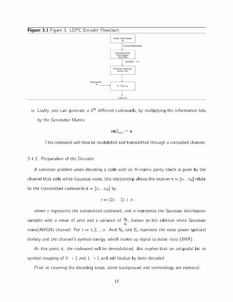
Figure 3.1 Figure 3. LDPC Encoder Flowchart

iv. Lastly, one can generate a 2M di�erent codewords, by multiplying the information bits

by the Generator Matrix:

mGsys = x

This codeword will then be modulated and transmitted through a corrupted channel.

3.1.3. Preparation of the Decoder

A common problem when decoding a code with an H-matrix parity check is given by the

channel that adds white Gaussian noise, this relationship allows the receiver r = [r1:::rN] relate

to the transmitted codewords c = [c1:::cN] by:

r = (2c� 1) + n

where c represents the transmitted codeword, and n represents the Gaussian distribution

samples with a mean of zero and a variance of No2Es

, known as the additive white Gaussian

noise(AWGN) channel. For t = 1,2,...,n. And No and Es represent the noise power spectral

density and the channel's symbol energy, which makes up signal to noise ratio (SNR).

At this point it, the codeword will be demodulated, this implies that an antipodal bit to

symbol mapping of 0! 1 and 1! 1 and will �nalize by been decoded.

Prior to covering the decoding steps, some background and terminology are essential.

15

In terms of probability, one says that the probability that a bit c�0; 1 has a �fty percent

probability of a bit being ipped when it goes through the channel. To further analyse this

context, the probability distribution is used by a parameter

p=Pr[c=1], since Pr[c=0]=1-p.

The conditional likelihood that c is a 0 or 1:

� = log P r [c=1P r [c=0]

= log p

1�p= log e�

Therefore, to retrieve p from �, e� = p

1�p, where p = 1

1+e��. The table below shows the

likelihood of � parameters, to recover p:

� = +&p(1) > p(0)

� = �&p(0) > p(1)

� = 0&p(0) = p(1)

� =1&p(1) = 1

� = �1&p(0) = 1

There are two types of probability density function been used, conditions pdf, is when c

is �xed and f( rc) is viewed as a function of r. The likelihood function is used when r is �xed,

then f( rc) is a function of c. Since Bayes rule is proportional to the likelihood function:

P r [c = 1 j r ] = f (r jc=1)P r [c=1]f (r)

Lets denote the likelihood functions as [15]

ft(1) = p(r j c = 1)

and

ft(0) = p(r j c = 0)

Thus, the log likelihood functions are given by

P r [c=1jr ][c=0jr ]

= log f (r jc=1)f (r jc=0)

+ log P r [c=1]P r [c=0]:

16

This function is known as the a posteriori probabilities (APP), the �rst term of the right

hand side is called the log likelihood ratio (LLR) and the second term of the right hand side

is a log probability ratio or a priori LLR.

If c has an equal probability of been zero or one, then a priori LLR is zero and the a

posteriori LLR is equal to the LLR, which is equal to

P r [c=1jr ][c=0jr ]

= log f (r jc=1)f (r jc=0)

, for Pr(c): 0 = Pr(c): 1

P r [c=1jr ][c=0jr ]

= 4Es

Nor

To note the changes, the "tanh rule" is needed for further explanation. Let �(c)�f0; 1gdeclare the parity of a set c = [c1:::cn] of n bits, this sets �(c) = 0when c has an even

number of ones and �(c) = 1 when c has an odd number of ones. If the binary random bits

are independent, then a priori LLR follows the tanh rule,

Proof the Tanh Rule, Let c = [c1:::cn]�f0; 1gn be a vector of n bits that are independent

but not equiprobable; let �i = log(P r [ci = 1]=P r [ci = 0]) declare the a priori LLR for the

i-th bit. Show that the priori LLR ��(c) = log(P r [phi(c) = 1)=P r [�(c) = 0]) for the parity

satis�es the tanh rule:

tanh(���(c)

2) =

∏ni=1 tanh(

��i

2)

(#)

Solving for previous equation for ��(c), generates the equivalent relationship of:

��(c) = �2 tanh(�1)(∏ni=1 tanh(

��i

2)):

and by manipulation of signs and magnitudes of LLR's (eq above) can be expressed as:

��(c) = �∏ni=1 sign(��i)f(

∑ni=1 f(j �i j));

which introduces the function:

f (x) = log ex+1ex�1

= � log(tanh(x=2)):

The function, f(x) is positive and decreases for x > 0, with f (0) = 1 and f (1) = 0.

Thus, f(x) = x for all x > 0.

17

Now, let c^ = c^1 :::c^n denote the value with the maximum likelihood,where c^i = 1i f �i >

0; elsec^i = 0. And the sign of ��(c) determines the most likely value of �(c), based of

�(c^),

sign(��(c)) = �∏ni=1 sign(��i) = �(�1)�(c^):

Therefore, when the sign is positive, the number is even and when the sign is negative,

the number �0is is odd.

The magnitude of the function ��(c) measures the accuracy that �(c) is its maximum

likely value. The magnitude is denoted as

j��(c)j = f(∑

i f(j�i j)) = f(f(j�i j)) = j�minj:

If certainty of the parity vector's bit, then magnitude of (��(c)) can be substituted in

(��(c)):

(��(c)) t �(�1)�(c^)j�minj:

The next section I will show how (��(c)) is used to decode codewords and how by using

the approximation of (��(c)) instead of (��(c)), a lower complexity is achieved.

A posteriori LLR is a detector that minimizes the error probability of the nth bit:

�n = log P r [cn=1jr ]P r [cn=0jrn]

�n = log P r [cn=1jr;fri 6=ng]P r [cn=0jrn;fri 6=ng]

;

following the above equation, if �n > 0 one can decide c^ = 1, otherwise c^ = 0.

One can also apply �n to Bayes rule,

P r [cn = 1jrnfri 6=ng =f(rn;cn=1;fri 6=ng)

f(rn;fri 6=ng)= f(rnjcn=1;fri 6=ng)f(cn=1;fri 6=ng)

f(rnjfri 6=ng)f(fri 6=ng)= f(rnjcn=1)P r [cn=1jfri 6=ng]

f(rnjfri 6=ng):

As shown, one states that cn, rn is independent of fri 6=ng.The �nal step to simplifying �n:

�n =f(rnjcn=1)P r [cn=1jfri 6=ng]f(rnjfri 6=ng)P r [cn=0jfri 6=ng

= log f(rnjcn=1)f(rnjcn=0)

+ log P r [cn=1jfri 6=ng]P r [cn=0jfri 6=ng]

= 2rnrn + log P r [cn=1jfri 6=ng]

P r [cn=0jfri 6=ng];

The �rst part on the right hand side, before the plus sign of �n is called intrinsic, meaning

that is the portion view from the nth channel and on the same right hand side of the equation,

18

after the plus sign is called extrinsic, which is proportional to the intrinsic but it is viewed by

others. Furthermore, the constant of 2=��2 is called channel reliability, which is the time

percentage a channel is free for use in a speci�c period based of scheduled available [33].

For the additive white gaussian noise (AWGN) is used the f(rn j cn) = (2���1=2)exp(�(rn�2cn + 1)2=(2�2)): [5]

For the previous equation of �n, it is introduce cn = �(c(i)) for all i = 1...j, because of a

j parity constraints of the code:

�n =2rnrn + log

P r [�(c(i))=1jf or i=1:::jjfri 6=ng]

P r [�(c(i))=1jf or i=0:::jjfri 6=ng]:

If the graph is cycle-free, the codeword vectors cn = [c1; c2; :::; cj] are conditionally in-

dependent given fri 6= ng and thereforeci components are conditionally independent given

fri 6= ng, this makes the equation above reduce to:

�n =2rnrn +�j

i=1��(c(i));

Finally, by substituting ��(c)(8)into�n above (20):

�n =2�2nrn � 2

∑j

i=1 tanh(�1)(∏k

l=2 tanh(��i ;l

2)):

Now, to decode a �nite number of codewords at the receiver, one must repetitively solving

the posteriori log which was �nalize to �n. The decoding algorithm I used for my code is as

follows:

Initialization {

� u(0)m,n = 0; f oral lm 2 f1; :::Mgandn 2 Nm;

� �(0)n = 2

�2nrn; f oral ln 2 f1; :::Ng.

Iteration { for iterations l = 1; 2; :::lmax :

� (Check to bit messages recovery) form 2 f1; :::Mgandn 2 Nm : u(l)m,n = �2 tanh�1(

∏i2Nm�n tanh(

��l�1i

+u(l - 1)m,i

2);

� (Bit to Check messages recovery) for n 2 f1; :::Ng : �(l)n = 2

�2nrn +

∑m 2 Mnu

(l)m,n:

Decision { At the last iteration of l, a hard decision is taken:

19

� if �n > 0c = 1,

� else c = 0.

[?]

3.1.4. Conclusion

This LDPC code facilitates a realization of parallel implementation based on the sparse

regular bipartite graph or Tanner graph, for whichM check nodes will be a separate processor,

and each N bit nodes is in a summing node. This makes it possible to use iteration in the

decoding to recover the original information message. This codes memory requirements

are low, with the exception when N bit nodes is large. This chapter described a serialized

implementation of a single check node processor that computes Mk check to bit messages

one by one since the LDPC codes remain active of research and have been applied to wireless

and satellite communication channels [15].

20

CHAPTER 4

REED SOLOMON

4.1. Introduction

In the early 1950s, Irving Reed and Gustave Solomon found a class of multiple cyclic error

correcting codes for non binary channels. And in the late 1950's, Bose and Ray Chudhurri and

Hocquenghem broaden the ideas of Hamming codes, by using Galois �eld theory to construct

t check symbols error correcting codes called BCH codes [7]. Since then, there has been

numerous researchers who have developed other important codes and have also developed

e�cient and fast decoding algorithms for these codes. Thanks to the creation of integrated

circuits, it has become a reality to implement complex codes in hardware and realize some

of the error correcting performance as Shannon's PH.D. dissertation of the channel capacity

theory was de�ned in 1960. Since then, Reed Solomon has been used for:

� deep space communications

� every day electronics

� wireless communications

� digital television

� satellite communications

� broadband modems

Such as, the all compact disc players include error correction circuitry based on two

interleaved (32, 28, 5) and (28, 24, 5), Reed Solomon codes that allow the decoder to

correct bursts of up to 4000 errors [7].

21

Figure 4.1 Figure 4. Linear Codes Family Tree

4.2. De�nition of Reed Solomon and Its Properties

A q-ary code is one with a prime number p and a power of p,q. These are codes from

the Galois �eld GF(q). Therefore, a code consist of a linear (n, k) with symbols from GF(q)

is a k-dimensional subspace of the vector space of all n-tuples over GF(q). This code is

generated by a polynomial of degree n - k with coe�cients from GF(q), this is a factor of

Xn � 1. The encoding and decoding process of the non-binary codes are similar to binary

codes. The length of a q-ary code is n = qs � 1, the positive integers are s and t. The

maximum this code can correct is less than t or t and it only need up to the 2nd parity check

digit. The roots � are a primitive element in the GF (qs), which are the coe�cients of the

generator polynomial g(X), these are the lowest degree of a t error correcting q-ary [18].

g(X) = LCMf�1(X); �2(X); :::; �2t(X)g:

When q = 2, then it is a binary code.

As shown in �gure 4, Reed Solomon is a special subclass of q-ary BCH codes, for which s

= 1, this is the most important subclass of q-ary BCH codes. To have a better understanding

of Reed Solomon codes, I will give a brief description of BCH codes and its de�nitions. The

parameter of a Reed Solomon code are:

� Block length n = q - 1

22

� Number of parity check digits: n - k = 2t

� Minimum distance: dmin = 2t+ 1:

In the next two section, an example of Reed Solomon encoder and decoder to will be

employed to describe the process for the implementation.

4.3. Preparation of the Encoder

To generate a generator matrix: Lets consider Reed Solomon codes with code symbols

with codes symbols from the Galois �eld GF (2m) meaning that q = 2m and � is a primitive

element in GF (2m). The generator polynomial of a primitive t error correcting Reed Solomon

code of length 2m � 1 is [18]:

g(X) = (X + �)(X + �2):::(X + �2t) = g0 + g1X + g2X2 + :::+ g2t�1X

2t�1 +X2t :

Evidently, g(X) has �;�2; :::; �2t as all its roots and has coe�cients from GF (2m). The

generated code by g(X) = (n; n�2t) cyclic code which consists of the polynomials of degree

n � 1 or less with coe�cients from GF (2m) that are multiples of g(X).

Encoding of this non binary code is similar to encoding a binary code, such that

a(X) = a0 + a1X + a2X2 + :::+ ak�1X

k�1

be the message to be encoded where k = n - 2t. In systematic form, the 2t parity check

digits are the coe�cients of the remainder b(X) = b0+b1X+ :::+b2t�1X2t�1 resulting from

dividing the message polynomial X2ta(X) by the generator polynomial g(X).

Let

v(X) = v0 + v1X + :::+ vn�1Xn�1

be transmitted [7].

4.4. Preparation of the Decoder

Let

r(X) = r0 + r1X + :::+ rn�1Xn�1

23

be the transmitters corresponding received vector codeword message. The error pattern is

added by the channel is

e(X) = r(X)� v(X) = e0 + e1X + :::+ en�1Xn�1

where the error is a symbol from GF (2m). Now, the location is important to know in

order to be able to correct the error received message bit or bits. The error location numbers

are de�ned as:

�l = �j l f or l = 1; 2; :::; v

For a binary q-ary, the decoder includes an additional step, lets consider a triple error

correcting Reed Solomon code with symbols from GF (24). The generator polynomial of this

code:

g(X) = (X + �)(X + �2)(X + �4)(X + �5)(X + �6) =

�6 + �9X + �6X2 + �4X3 + �14X4 + �14X4 +X6:

Let the all zero vector be the transmitted code vector and let r = (000�700�300000�400)

be the received vector. Thus, r(X) = �7X3 + �3X6 + �4X12:

To recover, there are four steps to follow:

i. The syndrome components are computed: S1 = r(�) = �10 + �9 + � = �12S2 =

r(�2) = �13+1+�13 = 1S3 = r(�3) = �+�6+�10 = �14S4 = r(�4) = �4+�12+�7 =

�10S5 = r(�5) = �5 + �3 + �4 = 0S6 = r(�6) = �10 + �9 + � = �12:

ii. Find the error location �(X) = 1 + �7X + �4X2 + �6X3:

iii. � Substitute 1, �;�2; :::; �14into�(X) :

� roots of �(X) : �3; �9and�12;

� reciprocal of roots: error pattern: �12�6�3

� error location: X3; X6; andX12:

iv. Z(X) = 1 + �2X +X2 + �6X3: [7]

24

4.5. Conclusion

Reed Solomon codes form a subclass of a very special of linear codes. Software-based

implementations of Reed Solomon codes are slower than hardware base implementations.

Reed-Solomon error correction code, is in reality slower but is good for recovery of errors.

25

CHAPTER 5

FOUNTAIN CODES

5.1. Introduction

Tornado codes began by research performed by Michael Luby, who founded the �rst

company in history named Digital Fountain who sold the software algorithms in forward error

correction codes, in speci�c he sold his invention which is classi�ed under Fountain Codes.

Later in the year 2000, Luby sold his company to Qualcomm and he is now the vice president

of the technical department in Qualcomm. Michael Luby's motivation of developing the

Tornado Code was because of his belief that erasure codes will become a key component

in protocols for reliable mass distribution of information [19]. Therefore Luby initiated the

development of more e�cient erasure codes with a goal of data transmission protocols in

a con icted setting where the loss pattern and latencies of packets are determined by a

con ict. This chapter describes the steps taken in the design, implementation and software

experimental performance of Tornado codes.

5.2. De�nition of Reed Solomon and its Properties

As stated by Luby's papers: "A digital fountain allows any number of heterogeneous clients

to get bulk data with optimal e�ciency at times of their scheduling. This classi�cation of

code guarantees a reliable delivery of date without the use of a feedback channel with a

boundary of high lose rates. The �rst protocol Luby developed that nearly approximates to

digital fountain codes is called tornado codes" [19].

26

Tornado codes are random linear codes that have rates very close to Shannon's channel

capacity. This forward error correction code software implementation runs orders of magni-

tude faster than the previous fastest. These codes are based on the development of multiple

layers of randomized irregular graphs for LDPC, with a �nal layer of Reed Solomon.

Lets go over some terminology used in this code:

� block length n of a code: is the number of symbols in the transmission.

� systematic code: the transmitted symbols can be divided into message symbols and

check symbols. One takes the symbols to be bits, and write a xor b to denote the

exclusive-or of bits a and b.

� message symbols: are chosen freely, depending on the length of H-matrix.

� check symbols: are computed from the message symbols.

� rate R of a code: is the ratio of the number of message symbols to the block length.

� encoder input: Rn message symbols

� transmits: n symbols

� all constructions, assume that the symbols are bits

Some parameters for this code are [28]:

� p fraction of symbols of each block

� n block length

� (1 - p)n fraction of the original rate

� pn redundant check symbols

This real time string of information data symbols are partitioned and transmitted in logical

unit of blocks. In the channel, unpredictable losses of at most p of fraction is possible from

symbols of each block in the network.

27

5.3. Preparation of the Encoder

In this section, the overall design is de�ned. There exist a code C(B) with n message

bits and �n check bits are part of a bipartite graph B. The graph B has n left nodes and �n

right nodes, that belong to the message bits and the check bits. C(B) is encoded by setting

each check bit to be the xor of its neighbouring message bits in the bipartite graph B. Hence,

the encoding time is proportional to the number of edges in B. The key of code is in the

design and analysis of the irregular bipartite graph B, for which there exist a repetition of the

decoding functions that recovers all the missing message bits [20].

5.4. Preparation of the Decoder

The way the decoder works is, it receives a binary value of a check bit and all but one of

the missing message bits that the codeword depends on. Then the missing message bit is set

to be the xor of the known check bit and its known message bits. The advantage of relying

on the xor recovery operation is that the complete decoding time is at the most proportional

to the number of edges in the graph. Luby's main technical innovation for this Tornado

code is in the design of random irregular graphs where the repetition of the xor operation is

guaranteed to recover all the message bits for the most part, if at most (1 � �)�n of the

message bits have been lost from the code C(B) [24].

Luby's Tornado code innovation is to construct codes that can recover from losses despite

of their location, he cascades C(B) codes by �rst using C(B) to produce �n check bits for

the original n message bits, he then uses a similar code to produce �2n check bits, which he

forms from C'(B) for the �n check bits and it beta can keep increasing. Finally, at the last

level, he uses what they call a conventional code for the loss resilience [3].

By constructing these sequence of codes C(B1); :::; C(Bm) from a sequence of graphs of

B0; :::; Bm, for which Bi consist of �in left nodes and on the right sides it has � i+1n nodes.

He selects m so that � i+1n is approximately pn and he ends the cascade layers of code with

28

a loss resilient code C of rate 1�� with � i+1n message bits that is recover from the random

loss of � fraction of its bits with high probability. And the code is �nalize to be de�ne:

C(B0; B1; :::; Bm; C), m message bits

�m+1i=1 �

in+ �m+2n=(1� �) = (n�=(1� �)

The check bits are formed by using C(B0) to produce �n check bits for the n message

bits, using C(Bi) to form � i+1n check bits. Assuming that the code C can be encoded and

decoded in quadratic time3, the code C(B0; B1; :::; Bm; C) can be encoded and decoded in

time linear in n. The process began by using the decoding algorithm for C to recover losses

that occur within its corresponding bits. If the code C recovers all the losses, then the

algorithm now knows all the check bits produced by C(Bm), which it can then use to recover

losses in the inputs to C(Bm). As the inputs to each C(Bi) were the check bits of (C(Bi�1),

I can work my way back up the recursion until I use the check bits produced by C(B0) to

recover losses in the original n message bits. If C can recover from the random loss of a

�(1� �) fraction of its bits with high probability, and that each C(Bi) can recover from the

random loss of a �(1 � �) fraction of its message bits with high probability, then it shows

that C(B0; B1; :::; Bm; C) is a rate 1 � � code that can recover from the random loss of a

�(1� �) fraction of its bits with high probability [22].

Thus, in the next section of this paper, graphs B are found so that the decoding algorithm

can recover from a �(1 � �) fraction of losses in the message bits of C(B), given all of its

check bits [16].

5.5. Degree Sequences of Irregular graph

A random bipartite graph with n left nodes and n� right nodes is speci�ed by the following

two sequences:

� Fraction of Edges of Degree i on left (�1;�2:::�m) : �i is the fraction of edges which

are occurrence on a node of degree i one the left side of the graph.

29

� Fraction of Edges of Degree i on right (�1; �2:::�m) : �i is the fraction of edges which

are occurrence on a node of degree i on the right side of the graph.

The check bit and node bit are de�ned as two polynomials over x 2 (0; 1]

�(x) =∑

i �ixi�1 �(x) =

∑i �ix

i�1

The results from the polynomial decoding process analysis are shown next. All of the

results, � is the probability that each input bit is lost independently of all other input bits.

i. A necessary condition on �, if the above simplistic decoding algorithm terminates suc-

cessfully is that �(1� ��(x)) > 1� x; f oral lx 2 (0; 1]

ii. If �(1���(x)) > 1�x; f oral lx 2 (0; 1], then for all � > 0, the decoding algorithm ter-

minates with at maximum �n message bits erased with probability 1�n2=3exp(� 3pn=2).

iii. If �1 = �2 = 0, then with probability 1�O(n�3=2), the recovery processes restricted to

the subgraph induced by any � fraction of the left nodes terminates successfully.

Through the third lemma condition of �1 = �2 = 0, and a set of di�erential equations,

the above results are derived. Researchers use the standard proofs on expander graphs to

show that the expansion condition holds with high probability and the decoding algorithm

terminates successfully [37].

5.6. Conclusion

The Tornado codes, an approximation to the ideal digital fountain protocol, have a de-

coding time linear in the input size, n but are block codes and are not suitable for multicasting

to a heterogenous class of receivers. Other fountain codes such as LT codes are rate less

codes, but they need decoding and encoding complexity of the order of O(k log(k)). Also,

Raptor codes have the advantages of LT codes and yet have a much better complexity. In

chapter 6, the Tornado code is applied.

30

CHAPTER 6

TORNADO CODE

6.1. Introduction

Michael Luby introduced the irregular Low Density Parity Check (LDPC)codes and called

it the Tornado code, which is a type of forward error correction (FEC) that corrects erasures

in high probability [21]. The creation of this code was to reduce the loss of data packets

in an IP network. The use of this code recovers lost packets from the packets that arrived

accurately at it destination. When the Tornado code is in comparison with other classes

of erasure codes such as Reed Solomon codes, the Tornado codes has faster encoding and

decoding speed. The recovery of the loss data is dependent on the bipartite (Tanner) graph,

for best results it is best to use cycle-free (Tanner) bipartite (Tanner) graphs [12].

The use of Tornado codes supports our design objectives of reliability, availability, and

performance:

� Reliability: the storage system should never lose data. By using Tornado codes, data

can be reconstructed in the event of multiple simultaneous disk drive failures.

� Availability: the storage system should be able to read and write data even during partial

hardware failure. By using Tornado codes, data can be retrieved from alternate devices

and reconstructed.

� Performance: the storage system should be capable of reading and writing data at a

su�cient throughput with respect to its capacity and user community. Tornado codes

use a linear-time coding method based on fast exclusive-or (XOR) operations,and can

encode and decode data quickly even in software.

31

6.1.1. Terminology

From Practical Loss Resilient Codes: "The block length of a code is the number of

symbols in the transmission. In a systematic code, the transmitted symbols can be divided

into message symbols and check symbols [10]. The Tornado code takes the symbols to be

bits, and write a⊕

b. The message symbols can be chosen freely, and the check symbols

are computed from the message symbols. The rate of a code is the ratio of the number of

message symbols to the block length [30]. For example, in a code of block length n and rate

R, the encoder takes as input Rn message symbols and produces n symbols to be transmitted.

In all of the Tornado codes constructions, it is assumed that the symbols are bits" [11].

6.1.2. Description of Codes

From the papers written by Luby, Mitzenmacher, Shokrollahi, and Spielman [35],[32],[31].

De�nition 1 The code C(B) corresponds to bipartite graph B with K left(message)

nodes and �k right(check) nodes (0 < � < 1), where each check node is the⊕

(XOR) of

its neighbours.

The Tornado code uses a sparse random graphs, for linear time encoding and decoding;

refer to chapter 2 for a description of the graphs. This code cascades codes of the form

C(B) to correct errors in both message bits and check bits.

De�nition 2 The code is family of codes C(B0toBt) constructed from graphs B0; :::; Bt ; whereBi

has � ik left nodes and � i+1k right nodes. Here t is chosen so that � i+1 tpk ;

A conventional code, such as Reed Solomon, corrects errors in C(Bt). Based on the value

chosen for parameter t, a slower conventional code will not a�ect overall linear time encoding

and decoding.

6.1.3. Encoding Rate

At the encoder of the Tornado code, it uses the modulo of the random bipartite graphs

Bi , beginning at the k message bits, the check bits from C(B0) are utilized as message bits

32

for C(B1). The check bit from C(B1) are utilized as message bits for C(B2), and so on if

the cascade is larger than three levels. The conventional code of Reed Solomon at the end

of the encoder, encodes the check bits of C(Bt) or in my case, it encodes the message bits

and check bit of C(B2) [13],[29]. The rate is approximately

k + �k + �2k + :::+ �k t (1� �)k:

Figures 5 and 6, below show a ow of how the bipartite graphs are cascaded and �nalize

with a conventional code at the end of the decoder.

Figure 6.1 Figure 5. Encoder and Decoder Cascade

33

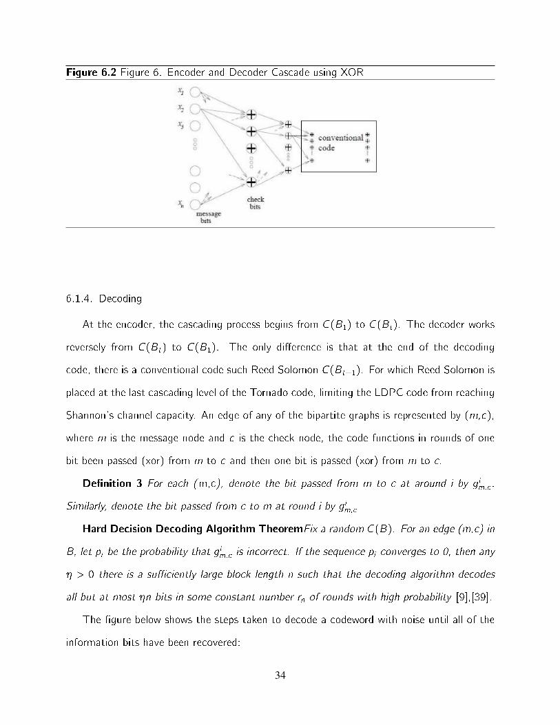
Figure 6.2 Figure 6. Encoder and Decoder Cascade using XOR

6.1.4. Decoding

At the encoder, the cascading process begins from C(B1) to C(Bt). The decoder works

reversely from C(Bt) to C(B1). The only di�erence is that at the end of the decoding

code, there is a conventional code such Reed Solomon C(Bt+1). For which Reed Solomon is

placed at the last cascading level of the Tornado code, limiting the LDPC code from reaching

Shannon's channel capacity. An edge of any of the bipartite graphs is represented by (m,c),

where m is the message node and c is the check node, the code functions in rounds of one

bit been passed (xor) from m to c and then one bit is passed (xor) from m to c.

De�nition 3 For each (m,c), denote the bit passed from m to c at around i by g im;c .

Similarly, denote the bit passed from c to m at round i by g im;c

Hard Decision Decoding Algorithm TheoremFix a random C(B). For an edge (m,c) in

B, let pi be the probability that gim;c is incorrect. If the sequence pi converges to 0, then any

� > 0 there is a su�ciently large block length n such that the decoding algorithm decodes

all but at most �n bits in some constant number rn of rounds with high probability [9],[39].

The �gure below shows the steps taken to decode a codeword with noise until all of the

information bits have been recovered:

34

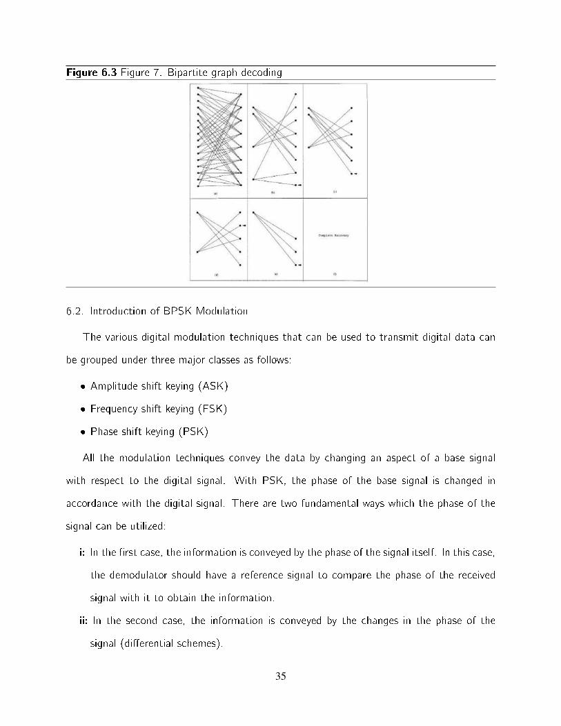
Figure 6.3 Figure 7. Bipartite graph decoding

6.2. Introduction of BPSK Modulation

The various digital modulation techniques that can be used to transmit digital data can

be grouped under three major classes as follows:

� Amplitude shift keying (ASK)

� Frequency shift keying (FSK)

� Phase shift keying (PSK)

All the modulation techniques convey the data by changing an aspect of a base signal

with respect to the digital signal. With PSK, the phase of the base signal is changed in

accordance with the digital signal. There are two fundamental ways which the phase of the

signal can be utilized:

i: In the �rst case, the information is conveyed by the phase of the signal itself. In this case,

the demodulator should have a reference signal to compare the phase of the received

signal with it to obtain the information.

ii: In the second case, the information is conveyed by the changes in the phase of the

signal (di�erential schemes).

35

A constellation diagram is used to conveniently represent the various PSK schemes. The

constellation diagram shows the points in z-plane where the real and imaginary axes are

replaced by the in-phase and quadrature phase components respectively. Based on this rep-

resentation, we can easily implement the modulation scheme. The amplitude of each point

along the in-phase axis is used to modulate a cosine (or sine) wave and the amplitude along

the quadrature axis to modulate a sine (or cosine) wave [29].

In PSK, the constellation points are positioned around a circle with uniform angular spacing

in order to obtain maximum phase separation between adjacent points to provide immunity

to corruption. In PSK scheme, the number of constellation points will be a power of 2 since

the data to be conveyed is binary. Binary phase shift keying (BPSK) is the simplest PSK

scheme. Two phases separated by 180o are used to implement the BPSK modulation. The

constellation diagram of the BPSK modulation is shown in Figure 8. It consists of two points

on the in-phase axis, one at 0o and the other at 180o , i.e. bit 0 is represented by the point

`-1' on the in phase axis and bit 1 is represented by the point `1' on the in-phase axis. BPSK

outperforms other PSK schemes since the separation between the constellation points is more

in case of BPSK. Figure 4.2 shows the performance of di�erent PSK schemes. However, it

is not suitable for high data rate applications or di�erent PSK schemes [29].

6.3. BPSK System Model

The system model for the BPSK modulation is the data to be modulated, which is sent.

In this block, the received bits are converted into k bit vectors. The converted vectors are

then sent to symbol mapper block. In this block, the bits are mapped to symbols: bit 0 is

mapped to -1 and bit 1 to 1 [29].

Figure 8, below shows the bits mapped to symbols through its conditional probability

density function:

36

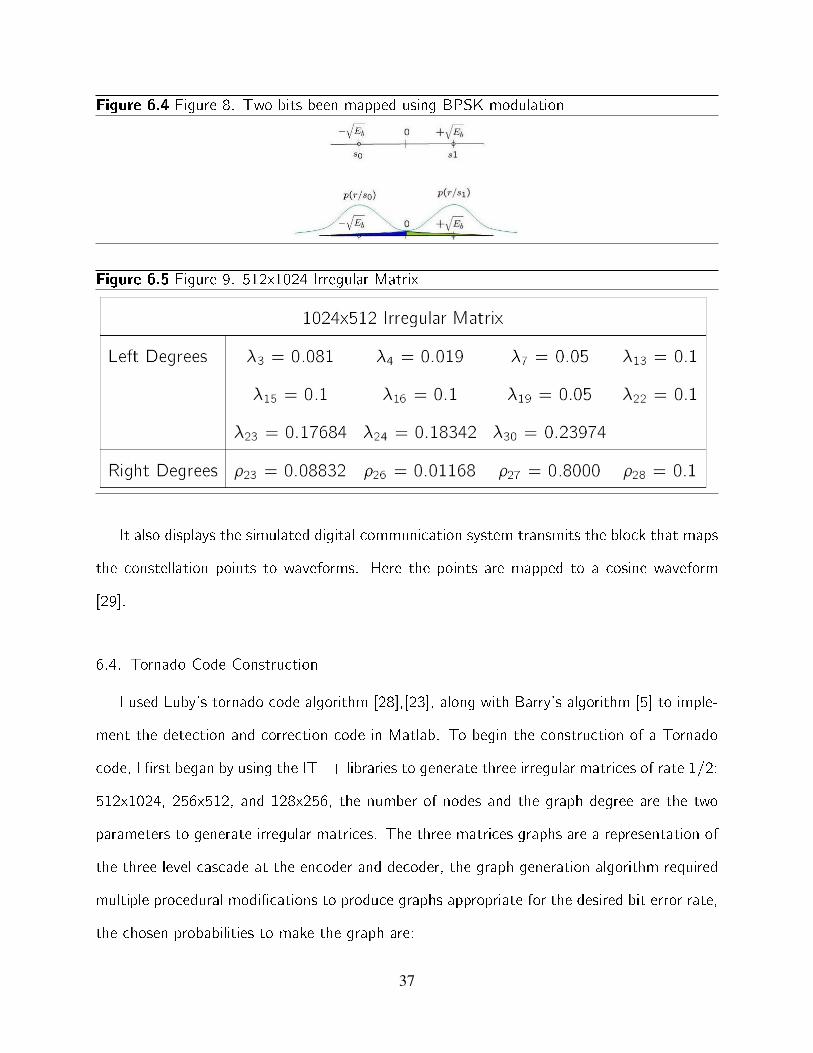
Figure 6.4 Figure 8. Two bits been mapped using BPSK modulation

Figure 6.5 Figure 9. 512x1024 Irregular Matrix

It also displays the simulated digital communication system transmits the block that maps

the constellation points to waveforms. Here the points are mapped to a cosine waveform

[29].

6.4. Tornado Code Construction

I used Luby's tornado code algorithm [28],[23], along with Barry's algorithm [5] to imple-

ment the detection and correction code in Matlab. To begin the construction of a Tornado

code, I �rst began by using the IT++ libraries to generate three irregular matrices of rate 1/2:

512x1024, 256x512, and 128x256, the number of nodes and the graph degree are the two

parameters to generate irregular matrices. The three matrices graphs are a representation of

the three level cascade at the encoder and decoder, the graph generation algorithm required

multiple procedural modi�cations to produce graphs appropriate for the desired bit error rate,

the chosen probabilities to make the graph are:

37

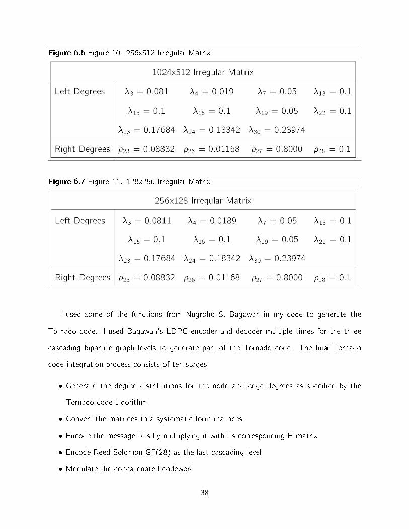
Figure 6.6 Figure 10. 256x512 Irregular Matrix

Figure 6.7 Figure 11. 128x256 Irregular Matrix

I used some of the functions from Nugroho S. Bagawan in my code to generate the

Tornado code. I used Bagawan's LDPC encoder and decoder multiple times for the three

cascading bipartite graph levels to generate part of the Tornado code. The �nal Tornado

code integration process consists of ten stages:

� Generate the degree distributions for the node and edge degrees as speci�ed by the

Tornado code algorithm

� Convert the matrices to a systematic form matrices

� Encode the message bits by multiplying it with its corresponding H matrix

� Encode Reed Solomon GF(28) as the last cascading level

� Modulate the concatenated codeword

38

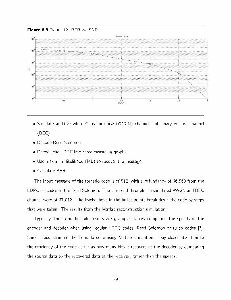
Figure 6.8 Figure 12. BER vs. SNR

� Simulate additive white Gaussian noise (AWGN) channel and binary erasure channel

(BEC)

� Decode Reed Solomon

� Decode the LDPC last three cascading graphs

� Use maximum likelihood (ML) to recover the message

� Calculate BER

The input message of the tornado code is of 512, with a redundancy of 66,560 from the

LDPC cascades to the Reed Solomon. The bits send through the simulated AWGN and BEC

channel were of 67,072. The levels above in the bullet points break down the code by steps

that were taken. The results from the Matlab reconstruction simulation:

Typically, the Tornado code results are giving as tables comparing the speeds of the

encoder and decoder when using regular LDPC codes, Reed Solomon or turbo codes [?].

Since I reconstructed the Tornado code using Matlab simulation, I pay closer attention to

the e�ciency of the code as far as how many bits it recovers at the decoder by comparing

the source data to the recovered data at the receiver, rather than the speeds.

39

CHAPTER 7

CONCLUSION

7.1. CONCLUSION AND FUTURE WORK

This thesis examined the application of tornado codes to archive forward error correction

code theoretical investigations to Matlab implementation. The resulting pro�led tornado

code simulations for additive white Gaussian (AWGN) show the e�ciency of the code, which

reaches below Shannon's channel capacity. In this paper each chapter covered a topic which

build up to construct the tornado code in the chapter 6. The tornado code simulation

technique that has been successfully used to determine how well a FEC expected to work when

transferring digital data streams. The goal of using this data to show how FEC optimizes a

digital data stream to gain a better digital communications systems was achieved. For future

for, to implement tornado code in hardware and research its capability of data storage over

a channel on real-world archival storage, to explore the higher bandwidth and low latency

capabilities of a high probable irregular graph. Also to set up a three location stations to

transfer data and record, tornado codes e�ciency versus timing versus storage capability.

40

APPENDIX A

IRREGULAR MATRIX GENERATOR

A.1. Libraries Installation

To generate irregular bipartite graphs, I use the open-source libraries at IT++ which is a

library in C++. This open-source library consists of classes and functions for mathematical,

signal processing and communication classes and functions. Its major use is in simulation

of communication systems and for research studies in communications systems. It is as well

used in areas such as machine learning and pattern recognition. The core of IT++ are generic

vector and matrices classes, which makes it similar to Matlab or GNU Octave. This library is

coded in C++. IT++ open source libraries increase accuracy, functionality and speed. The

libraries that can be used are BLAS, LAPACK, ATLAS and FFTW. The libraries compiler runs

in a Linux/GNU, BSD and UNIX systems environment, and on POSIX based environments

for Microsoft Windows such as Cygwin or MinGW with MSYS. Then installation of Ubuntu

was needed. Before going any further, it was necessary to download the GNU software. GNU

make, version 3.77 or later (check version with 'make version' or 'gmake version') GCC -

GNU Compilers Collection including C (gcc) and C++ (g++) compilers, version 3.3.x or

later (check version with 'gcc version') Then I downloaded 39 n t e x t g r e a t e r g z i p

cd i t p p <VERSION>. t a r . gz j t a r x f nn n t e x t g r e a t e r cd i t p p <VERSION>nn

n t e x t g r e a t e r b z i p 2 cd i t p p <VERSION>. t a r . bz2 j t a r x f nn n t e x t g r e

a t e r cd i t p p <VERSION>nn to i n s t a l l IT++. The commands w i l l u n t a r and

unpack t h e s o u r c e s , and e n t Next , t h e IT++ l i b r a r i e s a r e downloaded to c

r e a t e " Ma k e f i l e s " and c o n f i g n t e x t g r e a t e r . / c o n f i g u r e nn n t

e x t g r e a t e r make nn Modularization Modularization of the libraries is used to the con

41

gure script. The disable command will disable the packages that are not needed to be

installed. For instance, since this program is being used to generate an irregular bipartite

graph, the other library components that are not needed will not be downloaded; this is the

list below with the exception of 'Communications' module and 'Signal processing' module:

40 'disable-comm' - do not build the 'Communications' module 'disable-

xed' - do not build the 'Fixed-point' module 'disable-optim' - do not build the 'Numerical

optimisations' module 'disable-protocol' - do not include the 'Protocols' module 'disable-

signal' - do not build the 'Signal processing' module 'disable-srccode' - do not build the

'Source coding' module External Libraries Some of the con

gure scripts checks for some external libraries, which might be used by the IT++ library

(cf. IT++ Requirements). The detection procedure is as follows: (i) First, the presence of a

BLAS library among MKL, ACML, ATLAS and NetLib's reference BLAS is checked. If one

of the above mentioned can be used, HAVE BLAS is de

ned. (ii) Next, some LAPACK library is being searched, but only if BLAS is available. Full

set of LAPACK routines can be found in the MKL, ACML and NetLib's reference LAPACK

libraries. Besides, ATLAS contains a subset of optimised LAPACK routines, which can be

used with NetLib's LAPACK library (this is described in the ATLAS documentation). If some

LAPACK library can be found, HAVE LAPACK is de

ned. (iii) Finally, a set of separate checks for FFT libraries is executed. Currently three

dierent libraries providing FFT/IFFT routines can be used: MKL, ACML and FFTW. If at

least one of them is found, HAVE FFT id de

ned. Besides, one of the following: HAVE FFT MKL, HAVE FFT ACML or HAVE FFTW3

is de

ned, respectively. Now, depending on the environment of a system there are dierent ways

to con

42

gure its script for libraries: 41 If some external libraries are installed in a non-standard

location, as in MKL in '/opt/intel/ mkl/9.1', the 'con

gure' script will not detect them automatically. In such a case, you should use LDFLAGS

and CPPFLAGS environment variables to de

ne additional directories to be searched for libraries (LDFLAGS) and include

les (CPPFLAGS). For instance, to con

gure IT++ to link to 32-bit versions of MKL 9.1 external libraries, which is installed in

'/opt/intel/mkl/9.1' directory, you should use the following commands: n t e x t g r e a t e

r e x p o r t LDFLAGS="L/ opt / i n t e l /mkl /9.1/ l i b /32 " nn n t e x t g r e a t e r e

x p o r t CPPFLAGS="I / opt / i n t e l /mkl /9.1/ i n c l u d e " nn n t e x t g r e a t e

r . / c o n f i g u r e nn I n s t e a d o f CPPFLAGS , one can us e 'wi thf f t i n c l u d

e=<PATH>' c o n f i g u r e o I n t h e case t h a t e x t e r n a l l i b r a r i e s hav e nons t

a n d a r d names , e . g . ' l i b b l a n t e x t g r e a t e r . / c o n f i g u r e wi thb l a

s="l a t l a s l b l a s "nn If there is only one library speci

ed, you can use a simpli

ed notation without the preceding '-l', e.g. 'with-t=tw3' instead of 'with-tw=-ltw3'. The

con

gure script provides a new 'with-zdotu=<method>' option. It can be used to force the

default calling convention of BLAS 'zdotu ' Fortran function. The BLAS libraries 42 built

with g77 compiler do not return the complex result of a function; instead, they pass it via

the

rst argument of the function. By using 'with-zdotu=void' option, this approach can

be forced (g77 compatible). On the other hand, the libraries built with a newer gfortran

compiler return the complex result like a normal function does, but calling such interface from

C++ is not portable, due to incompatibilities between C++ complex<double> and Fortran's

COMPLEX. Therefore in such case a Fortran wrapper function 'zdotusub::' can be used

43

('with-zdotu=zdotusub'), however it requires a working Fortran compiler. By default, IT++

tries to guess the proper method based on the detected BLAS implementation. For instance,

the BLAS library provided by Intel MKL works

ne with the 'void' method. Eventually, if no Fortran compiler is available and the 'void'

method can not be used, the zdotu BLAS function is not used at all and a relevant warning

message is displayed during the con

guration step. Although it is not recommended, you can intentionally prevent detec-

tion of some external libraries. To do this you should use 'without-<LIBNAME>' or 'with-

<LIBNAME>=no', e.g.: n t e x t g r e a t e r . / c o n f i g u r e wi t h o u t b l a s wi t h

o u t l a p a c k nn end f l s t l i s t i n g g nemphf Op t imi z a t i o n F l a g s g I t++

recommends to s e t t h e CXXFLAGS e n v i r o nme n t v a r i a b l e wi t h some c omp i

n t e x t g r e a t e r CXXFLAGS="DNDEBUG O3 march=pent ium4 p i p e " . / c o n f i

g u r e nn 43 I n t h e case o f Sun ' s UltraSPARC 64 b i t p l a t f o rm and GCC c omp

i l e r , t h e f l n t e x t g r e a t e r e x p o r t CXXFLAGS="DNDEBUG O3 mcpu=v9

m64 p i p e "nn n t e x t g r e a t e r . / c o n f i g u r e nn If CXXFLAGS is not set in the

environment, it will be initialized with the default ags, i.e. "-DNDEBUG -O3 -pipe". Con

guration Status After the con

guration process is

nished, a status message is displayed. For example, after calling the following con

guration command n t e x t g r e a t e r . / c o n f i g u r e wi thb l a s="l b l a s " nn

on a r e c e n t Gentoo L i n u x s y s t em wi t h b l a s a t l a s , l a p a c k a t l a s and f

f tw p i t p p 4.0.3 l i b r a r y c o n f i g u r a t i o n : Directories: - pre

x ......... : /usr/local - exec. pre

x .... : pref ix includedi r::::: :pre

x/include - libdir ......... : 44 exec:under scorel ine:pref ix=l ib datarootdi r:::: :pre

44

x/share - docdir ......... : datarootdi r=doc=PACKAGE. TARNAMESwitches : �debug:::::::::: :no�exceptions::::: : no�html�doc::::::: : yes�shared::::::::: : yes�static::::::::: : no�expl icitdeps:: : no � zdotu:::::::::: : zdotusubDocumentationtools : �doxygen:::::::: :yes � latex:::::::::: : yes � dv ips:::::::::: : yes � ghostscr ipt:::: : yesTestingtools :

�di ::::::::::: : yesOptionalmodules : �comm::::::::::: : yes�xed .......... : yes - optim .......... : yes - protocol ....... : yes - signal ......... : yes - srccode

........ : yes External libs: - BLAS ........... : yes * MKL .......... : no * ACML ......... : no *

ATLAS ........ : yes - LAPACK ......... : yes - FFT ............ : yes * MKL .......... : no * ACML

......... : no * FFTW ......... : yes Compiler/linker ags/libs/defs: - CXX ............ : g++ - F77

............ : gfortran - CXXFLAGS ....... : -DNDEBUG -O3 -pipe - CXXFLAGS.underscore

line.DEBUG . : - CPPFLAGS ....... : - LDFLAGS ........ : - LIBS ........... : -ltw3 -llapack

-lblas ||||||||||||||||||||- Now type 'make make install' to

build and install itpp-4.0.3 library ||||||||||||||||||||- Compi-

lation Now, it is time for compiling and linking the IT++ library. To do so, please simply run

the following command: n t e x t g r e a t e r make nn 45 IT++ shall compile without any

errors or warnings. Testing the Compiled Library To check if ones library has been compiled,

linked properly and that it works as expected ! Execute the following testing process: n t e

x t g r e a t e r make che c k nn As a r e s u l t , you s h o u l d o b t a i n a s i m i l a r r e

p o r t : Tes t ' a r r a y n t e s t ' PASSED. Tes t ' b e s s e l n t e s t ' PASSED. [ . . . ]

Tes t ' window n t e s t ' PASSED. Tes t ' h i s t o g r am n t e s t ' PASSED. Tes t ' s t

a t n t e s t ' PASSED. 46 g Check if all the executed tests PASSED. If not, please report

the problem on the IT++ Help forum. Installation Finally, you should install the compiled

and linked library, include

les and HTML documentation (optionally) by typing: n t e x t g r e a t e r make i n s t

a l l Depending on t h e PREFIX s e t t i n g s d u r i n g c o n f i g u r a t i o n , you might

need t h E v e n t u a l l y , you might i n v o k e t h e f o l l o w i n g command n t e x t g

45

r e a t e r make c l e a n to remove a l l f i l e s c r e a t e d d u r i n g c omp i l a t i o n p

r o c e s s , or e v en n t e x t g r e a t e r make d i s t c l e a n 47 to remove all

les generated by the 'con

gure' script. After the installation has completed you are able to brows ip++ libraries and

compile any of the source codes you are interested in getting further information in. How I

generated my code was by using the c written

le of LDPC codes and I modi

ed it to work for the matrix that I need of 1024x512, 512x256 and 256x128; is found in

the Appendix.

A.2. Generate Irregular Code

/ // Ge n e r a t e some e xampl e LDPC cod e s / i n c l u d e <i t p p / itcomm .

h> i n c l u d e <i o s t r e am > u s i n g namespace i t p p ; u s i n g namespace s t d ;

BPSK t e s t ; i n t main ( ) f // 10000 b i t s ( t a k e s a few mi n u t e s to run ) cout <<

"========= IRREGULAR CODE 10000 BITS ==========" << e n d l ; LDP C

P a r i t y I r r e g u l a r H; LDP C P a r i t y I r r e g u l a r H1 ; 48 LDP C P a r i t y I r r

e g u l a r H2 ; H. g e n e r a t e (1024 , "0 0 0.081 0.019 0 0 0 .0 5 0 0 0 0 0 0 . 1 0 0 . 1

0 . 1 0 0 0 .0 5 0 0 0 . 1 0.17684 0.18342 0 0 0 0 0 0.23974 " , "0 0 0 0 0 0 0 0 0 0 0 0 0

0 0 0 0 0 0 0 0 0 0.08832 0 0 0.01168 0.8000 0 . 1 " , " r a n d " , // random u n s t r u

c t u r e d ma t r i x " 500 8" ) ; // o p t imi z e g i r t h H1 . g e n e r a t e (512 , "0 0

0.0802 0.0198 0 0 0 .0 5 0 0 0 0 0 0 . 1 0 0 . 1 0 . 1 0 0 0 .0 5 0 0 0 . 1 .17684 0.18342

0 0 0 0 0 0.23974 " , "0 0 0 0 0 0 0 0 0 0 0 0 0 0 0 0 0 0 0 0 0 0 0.08832 0 0 0.01168

0.8000 0 . 1 " , " r a n d " , // random u n s t r u c t u r e d ma t r i x " 500 8" ) ; // o p

t imi z e g i r t h H2 . g e n e r a t e (256 , "0 0 0.0811 0.0189 0 0 0 .0 5 0 0 0 0 0 0 . 1 0

0 . 1 0 . 1 0 0 0 .0 5 0 0 0 . 1 .17684 0.18342 0 0 0 0 0 0.23974 " , "0 0 0 0 0 0 0 0 0 0

0 0 0 0 0 0 0 0 0 0 0 0 0.08832 0 0 0.01168 0.8000 0 . 1 " , " r a n d " , // random u n s

46

t r u c t u r e d ma t r i x 49 " 500 8" ) ; // o p t imi z e g i r t h / LDPC Code C(H) ; /

C. s a v e c o d e (" RU 10000 . i t " ) ; / GF2mat spar s e M = H. ge t H ( f a l s e ) ;

GF2mat spar s e M1 = H1 . ge t H ( f a l s e ) ; GF2mat spar s e M2 = H2 . ge t H ( f a

l s e ) ; H. d i s p l a y s t a t s ( ) ; cout << " The ma t r i x has "<< M. rows ( ) << " rows

. "<< e n d l ; cout << " The ma t r i x has "<< M. c o l s ( ) << " colums . " << e n d l ; i n t

count =0; f o r ( i n t i =0; i < M. rows ( ) ; i++) f count =0; f o r ( i n t j =0; j<M. c o l s

( ) ; j++) f cout << H. g e t ( i , j ) << " " ; i f (H. g e t ( i , j )==1) count++; g cout << "

" << count ; cout << e n d l ; 50 g cout << e n d l ; cout << e n d l ; cout << e n d l ; cout << e n

d l ; cout << e n d l ; cout << " The ma t r i x 1 has "<< M1. rows ( ) << " rows . "<< e n d l ;

cout << " The ma t r i x 1 has "<< M1. c o l s ( ) << " colums . " << e n d l ; f o r ( i n t i =0;

i < M1. rows ( ) ; i++) f count =0; f o r ( i n t j =0; j<M1. c o l s ( ) ; j++) f cout << H1 .

g e t ( i , j ) << " " ; i f (H1 . g e t ( i , j )==1) count++; g cout << " " << count ; cout << e

n d l ; 51 g cout << " The ma t r i x 2 has "<< M2. rows ( ) << " rows . "<< e n d l ; cout << "

The ma t r i x 2 has "<< M2. c o l s ( ) << " colums . " << e n d l ; f o r ( i n t i =0; i < M2.

rows ( ) ; i++) f count =0; f o r ( i n t j =0; j<M2. c o l s ( ) ; j++) f cout << H2 . g e t ( i

, j ) << " " ; i f (H2 . g e t ( i , j )==1) count++; g cout << " " << count ; cout << e n d l ; g

r e t u r n 0 ; g

47

APPENDIX B

TORNADO CODE

c l c ; c l e a r a l l ; M = 5 1 2; N = 1024; M1 = 2 56 ; N1 = 51 2 ; M2 = 1 28 ; N2

= 25 6 ; Na l l = 67072; n oCy c l e = 1 ; s t r a t e g y = 2 ; 53 EbN0 = [1 .5 0 . 5 1 1 .

5 2 2 . 5 3 3 . 5 4 4 . 5 5 ] ; i t e r = 2 0 ; f rame = 5 0 ; m = 8 ; n=2m1; k = 1;H1 =

open(0matlabb:mat 0);H = H1(:; :):ans;H2 = open(0i r regular256x512:mat 0);Hm = H2(:

; :):B;H3 = open(0i r regular128x256:mat 0);H2 = H3(:; :):C; f or i = 1 : length(EbN0)54ber4(i) =

0; dSource = round(rand(M; f rame)); f pr intf (0F rame : [c; newH] = makePar ityChk(dSource(:

; j); H; strategy); u(:; j) = [c ; dSource(:; j)]; dSource1(:; j) = u(1 : 256; j); [c1; newH1] =

makePar ityChk1(dSource1(:; j); Hm; strategy); u1(:; j) = [c1; dSource1(:; j)]; dSource2(:

; j) = u1(1 : 128; j); [c2; newH2] = makePar ityChk(dSource2(:; j); H2; strategy); u2(:

; j) = [c2; dSource2(:; j)]; 55lastlayer(:; j) = RSenc((u2(:; j))0; m; n; k); convert = lastlayer ; f inalcodeword =

vertcat(u; u1; u2; convert); bpskModF INAL = 2f inalcodeword1;N0 = 0:5=(exp(EbN0(i)log(10)=10)); txF INAL(:

; j) = bpskModF INAL(:; j)+sqrt(N0)randn(size(bpskModF INALf orr r = 1 : Nal l i f txF INAL(r r; j) <

0bpskDemodF INAL(r r; j) = 0; elsebpskDemodF INAL(r r; j) = 1; endenddecout = length(bpskDemodF INAL)length(u)length(u1)length(u2); 56decout2 =

bpskDemodF INAL(1793 : 67072; j); r sDEC(j; :) = RSdec(decout2; n; k;m); vhat2(j; :

) = decodeLogDomainSimple((r sDEC(j; :))0; newH2; i ter); vhat3input(j; :) = horzcat((vhat2(j; 129 :

256)); (bpskDemodF INAL(1153 : vhat3(j; :) = decodeLogDomainSimple(vhat3input(j; :

)0; newH1; i ter); vhat4input(j; :) = horzcat((vhat3(j; 1 : 512)); (bpskDemodF INAL(513 :

102vhat4(j; :) = decodeLogDomainSimple((vhat4input(j; :))0; newH; iter)[num4; rat4] =

biter r((vhat4(j; :))0; u(:; j)); ber4(i) = (ber4(i)+rat4); vhat22(:; j) = vhat2(j; 129 : 256); vhat33(:

; j) = vhat3(j; 257 : 512); vhat44(:; j) = vhat4(j; 513 : 1024); end57ber4(i) = ber4(i)=f rame; f i rer ror(i ; :

) = sum(r sDEC 0 = u2); secer ror(i ; :) = sum(u1(1 : 128; :) = (vhat2(:; 129 : 256))0); er rorsintr(i ; :

48

) = sum(bpskModF INAL(1 : 1024; :) = bpskDemodF INAL(1 : 102er rorsintr1(i ; :) =

sum(bpskModF INAL(1025 : 1536; :) = bpskDemodF INAL(1er rors1(i ; :) = sum(vhat33 =

dSource1); er rorsintr2(i ; :) = sum(bpskModF INAL(1537 : 1792; :) = bpskDemodF INAL(1er rors2(i ; :

) = sum(vhat22 = dSource2); er rorsintr2f (i ; :) = sum(bpskModF INAL = bpskDemodF INAL); er rors2f (i ; :

) = sum(vhat44 = dSource); enderr f ra = sum(er rors2f 0):=f rame; ber = er r f ra:=M; 58hold ; semi logy(EbN0; ber4;0 o 0); gr idon; holdof f ;

49

BIBLIOGRAPHY

[1] discrete-structures@ONLINE, march 2011.

[2] Mitchell Abigail and Rosenthal Joachim, Design of irregular graphs for erasure decoding,

IEEE 18 (2008), no. 2, 208{584.

[3] M. Luby N. Alon, A linear time erasure-resilient code with nearly optimal recovery, IEEE

Transactions on Information Theory 42 (1996), no. 6, 1732{1736.

[4] Iryna Andriyanova and Jean-Pierre Tillich, Designing a good low-rate sparse-graph code,

France Telecom R and D (2006).

[5] John R. Barry, Low density parity-check codes, Georgia Institute of Technology (2001).

[6] Thomas M. Cover and Joy A. Thomas, Graph theory, 2003.

[7] , Elements of information theory, Second Edition, no. 146, John Wiley and Sons,

Inc., Hoboken, New Jersey, 2006.

[8] Doxygen, discrete-structures@ONLINE, september 2010.

[9] Y. Y. Tai et al. L. Lan, A trellis-based method for removing cycles from bipartite graphs

and construction of low density parity check codes, IEEE Communications (2004), no. 8,

443{445.

[10] M. Mitzenmacher et al. M. Luby, E�cient erasure correcting codes, IEEE TRANSAC-

TIONS ON INFORMATION THEORY 47 (2001), no. 2, 569{584.

[11] Hakim Weatherspoon et al. Matthew Delco, Typhoon: An archival system for tolerat-

ing high degrees of �le server failure, http://www.cs.cornell.edu/ hweather/Typhoon/,

1999.

50

[12] Micheal Mitzenmacher et al. Michael Luby, Analysis of low density parity check codes and

improved designs using irregular graphs, Proceedings of the 30th ACM STOC Dallas,

TX (1998), 249{258.

[13] Saied Hemati et al. Mohammad R. Yazdani, Improving belief propagation on graphs with

cycles, IEEE Letters 8 (2004), 57{59.

[14] R. G. Gallager, Low density parity codes, MIT Press, Cambrige, MA (1963).

[15] Metha Gayatri, Ldpc, Professor Thesis.

[16] J. Bl mer J. Edmonds M. Luby M. Sudan A. Albanese, Priority encoding transmission,

IEEE Transactions,on Information Theory 42 (1996), no. 6, 1737{1744.

[17] D. Sridhara C. A. Kelley and J. Rosenthal, Tree-based construction of ldpc codes having

good pseudocode-word weights, IEEE Trans. Information Theory 53 (2007), no. 4,

1460{1478.

[18] Shu Lin and Daniel J. Costello Jr., "error control coding, fundamentals and applications",

series = Second Edition, publisher = Prentice-Hall,Inc., Englewood Clivts, year = 1983.

[19] Michael Luby, Michael luby's page, March 2003.

[20] John W. Luby Michael G. Mitzenmacher Michael Byers and Ashutosh Rege, A digital

fountain approach to reliable distribution of bulk data, Tech. report, Digital Foundation,

1987.

[21] Chang Yilin Luo Zhong Wang Jing Ai Da, Practical algorithms for tornado codes, Journal

of Electronics(China) (2006), 274{276.

[22] J. Edmonds M. Luby N. Alon, Linear time erasure codes with nearly optimal recovery,

Proc. of the 36th Annual Symp. on Foundations of Computer Science (1995).

[23] Cambridge Univ. MacKay, D.J.C.; Cavendish Lab., Good error correcting codes based

on very sparse matrices, IEEE TRANSACTIONS ON INFORMATION THEORY 45

(1999), no. 2, 399{431.

51

[24] David J.C. MacKay, Information theory, inference, and learning algorithms, Second Edi-

tion, Cambridge University Press, 2003.

[25] B. Marcus and editors J. Rosenthal, Codes, systems and graphical models, Springer-

Verlag, 2001.

[26] Ardakani Masoud and Frank R. Kshcischang, A more accurate one-dimensional analysis

and design of irregular ldpc codes, IEEE 52 (2004), no. 12, 2106{2114.

[27] Michael G. Mitzenmacher Michael Shokrollahi M. Amin Luby and Daniel A. Spielman,

Analysis of low density codes and improved designs using irregular graphs, STOC.

[28] Michael G. Mitzenmacher Michael Shokrollahi M. Amin Spielman Daniel A. Luby and

Volker Stemann, Practical loss-resilient codes, Proc. 29th Symp. on Theory of Comput-

ing (1997), 150{159.

[29] J.G. Proakis, Digital communications, Fourth Edition, McGraw-Hill,, 2000.

[30] A recursive approach to low complexity codes R. M. Tanner, Design of capacity-

approaching irregular low-density parity-check codes.

[31] M. A. Shokrollahi T. Richardson and R. Urbanke, Design of capacity-approaching irreg-

ular low-density parity-check codes.

[32] T. Richardson and R. Urbanke, The capacity of low-density parity check codes under

message-passing decoding, IEEE Trans. Inform. Theory 47 (2000), 599{618.

[33] Jr.; Richardson T.J.; Urbanke R. Sae-Young Chung; Forney, G.D., On the design of low-

density parity-check codes within 0.0045 db of the shannon limit, IEEE Communications

Letters 5 (2001), no. 2, 58{60.

[34] R.L. Sae-Young Chung; Richardson, T.J.; Urbanke, Analysis of sum-product decoding

of low-density parity-check codes using a gaussian approximation,, IEEE Trans. Inform.

Theory 47 (2001), no. 2, 657{670.

52

[35] Mitzenmacher Michael Shokrollahi M. Amin Luby Michael G. and Spielman Daniel A,

Improved low-density parity-check codes using irregular graphs, IEEE TRANSACTIONS

ON INFORMATION THEORY 47 (2001), no. 2, 585.

[36] R. Smarandache and P. O. Vontobel, Pseudo-codeword analysis of tanner graphs from

projective and euclidean planes, IEEE Trans. Inform. Theory 53 (2007), no. 7, 2376{

2393.

[37] D. Spielman, Linear-time encodable and decodable error- correcting codes, IEEE Trans-

actions on Information Theory 42 (1996), no. 6, 1723{1731.

[38] Madhu (Instructor) Sudan, Algorithmic introduction to coding theory, March, Course

6.897.

[39] H. Stephan Wenger, 264/avc over ip, IEEE Trans. on Circuits and Systems for Video

Technology 13 (2003), no. 7, 645{656.

[40] L.; Djurdjevic I.; Lin S.; Abdel-Gha�ar K. Xu, J.; Chen, Construction of regular and

irregular ldpc codes: Geometry decomposition and masking, IEEE Transactions on In-

formation Theory 53 (2007), no. 1, 121{134.

53