MATLAB tool for evaluating the symmetry of the forehead in patients

with unicoronal synostosis before and after operation.

Master of Science Thesis in Radiation Physics

Author: Annelie Lindström

1/23/2011

Supervisors: Peter Bernhardt, Lars Kölby and Jacob Heydorn-Lagerlöf

DEPARTMENT OF RADIATION PHYSICS

UNIVERSITY OF GOTHENBURG GOTHENBURG, SWEDEN

1

Abstract Unicoronal synostosis is a condition where one of the coronal sutures, in an infant’s skull,

has prematurely fused. This will result in a deformed skull where the forehead is flattened on the ipsilateral side and bulges outwards on the contralateral side.

The craniofacial unit at the Department of Plastic Surgery at Sahlgrenska University has

continuously improved craniofacial surgery over the years. The aim of this project was to

develop a MATLAB tool that evaluates the symmetry of the forehead in patients with

unicoronal synostosis before and after treatment. The program will be used as a quantitative

measure in a study for craniofacial surgery.

The program evaluates CT images and cephalometry images of the skull. The cranium is

segmented leaving only the uttermost edge of the cranium and the symmetry between the

left and right side of the forehead is evaluated. By calculating the symmetry of the forehead

before and after operation a quantitative measure of the outcome is achieved, and the

treatment can be evaluated.

The symmetry of symmetrical phantoms, both circular and elliptical, has been evaluated and

the result shows that it is completely symmetrical. 15 pre-operative images and 15 post-

operative images have also been evaluated and it is shown that the relative standard

deviation increases for a more symmetrical cranium. The results achieved for the CT images

have a lower relative standard deviation than the results achieved for the cephalometry

images. The success of the operations has been evaluated with two different equations. One

method calculates the absolute change and the other calculates the relative change. The

relative change is demonstrated to be a better evaluation of the operation.

2

Table of Contents 1 Introduction ............................................................................................................................ 4

2 Theory ..................................................................................................................................... 5

2.1 Digital image ..................................................................................................................... 5

2.2 Digital image processing ................................................................................................... 6

2.2.1 Histogram processing ................................................................................................ 6

2.2.2 Spatial filtering .......................................................................................................... 7

2.2.3 Segmentation ............................................................................................................ 8

2.3 MATLAB ............................................................................................................................ 8

3 Method .................................................................................................................................... 8

3.1 CT images ....................................................................................................................... 10

3.1.1 Definition of center-point, end-point, and unfused side ........................................ 11

3.1.2 Segmentation .......................................................................................................... 11

3.2 Cephalometry images ..................................................................................................... 13

3.2.1 Contrast enhancement ............................................................................................ 13

3.2.2 Definition of center-point, end-point, and unfused side ........................................ 13

3.2.3 Interactive definition of the cranium ...................................................................... 13

3.3 Dividing the skull into two parts, one left and one right ............................................... 13

3.4 Calculation of the symmetry between the two sides .................................................... 15

3.5 Evaluation of the program ............................................................................................. 17

3.5.1 Symmetry evaluation .............................................................................................. 17

3.5.2 Test on symmetrical phantoms ............................................................................... 18

3.5.3 The certainty of the program .................................................................................. 19

4 Results ................................................................................................................................... 19

4.1 Symmetry evaluation ..................................................................................................... 19

4.2 Test on symmetrical phantoms ...................................................................................... 19

4.3 The certainty of the program ......................................................................................... 20

5 Discussion .............................................................................................................................. 22

6 Conclusions ........................................................................................................................... 25

Acknowledgements ................................................................................................................. 26

References................................................................................................................................ 27

3

Appendix .................................................................................................................................. 28

Appendix I ............................................................................................................................. 28

Appendix II ............................................................................................................................ 35

4

1 Introduction The bones in an infant’s skull are joined together by six sutures, a type of fibrous joint [1].

These sutures make it possible for the skull to compress when passing through the birth

canal. They also allow the skull to expand when the brain grows. The infant’s skull grows

rapidly and at one year of age the brain has tripled its volume. The rapid growth requires the

cranium to be able to expand. As the child gets older, and the growth of the brain is

decreased, the sutures will fuse one by one.

In a condition called craniofacial synostosis the sutures can fuse prematurely, days or

months before birth. For these children the skull won’t be able to grow at the affected

suture. To compensate for the prematurely fused suture the unaffected sutures will grow in

a different pattern compared to a normal skull, resulting in an abnormal shape. Depending

on which suture has been fused the shape of the skull will have special features. Usually one

suture is closed too early but sometimes several sutures can be closed simultaneously.

The coronal suture separates the parietal and the frontal bones (Figure 1). For patients with

unicoronal synostosis one of the coronals is prematurely closed [2] [3]. Unicoronal synostosis

is characterized by an asymmetric forehead. On the ipsilateral side, the side where the

suture has fused, the forehead is flattened and on the contralateral side the forehead bulge

outwards. The face is also affected due to the abnormal shape of the forehead. The eye and

the eyebrow may be pushed downward by the bulging forehead [4].

Figure 1. Image of the cranium and its sutures where the arrow points to the coronal suture [5].

5

The craniofacial unit at the Department of Plastic Surgery at Sahlgrenska University has a

large material of patients with synostosis. At the department many new methods in

craniofacial surgery have been developed over the years. An example of a new treatment

modality is stainless steel wires for implantation, which was introduced by the Gothenburg

craniofacial team eleven years ago. These wires affect and guide the dynamic growth of the

infant’s skull. When the growth of the brain is directed and affected by the wires the skull

shape is forced into normality.

Today the result of an operation is evaluated by studying the patient’s skull and at the x-ray

images of the patient. However, this is a result that will depend on the evaluator. Therefore

a quantitative measure of the result, independent of the viewer, is preferable. A quantitative

measure of the symmetry of the skull would make it possible to compare and evaluate, for

example, different surgical procedures.

The aim of this project was to develop a MATLAB tool that calculates the symmetry of the

forehead in patients with unicoronal synostosis before and after treatment. This should be

done by comparing the left and the right side of the forehead in both computed tomography

(CT) and cephalometry images. The program will be used as a quantitative measure in a

study where two different treatments are compared.

2 Theory

2.1 Digital image An image can be defined as a two-dimensional function f(x,y), where x and y are spatial

coordinates. The intensity or gray level at the point (x,y) is the amplitude of f. It is a positive

number whose value is determined by the source of the image. A digital image make up of a

finite number of elements, each element has a particular location determined by the

coordinates x and y, and a finite value. These elements are called picture elements also

known as pixels.

A digital image is stored as a two-dimensional array, a matrix, where the columns and rows

corresponds to the spatial coordinates x and y respectively [6]. A digital image of size M x N

can be represented as shown in equation 1.

( ) [ ( ) ( )

( ) ( )] (1)

6

2.2 Digital image processing Digital image processing refers to processing digital images with a computer using

mathematical algorithms. The basics of digital image processing are to enhance an image so

that the result suits a specific application more than the original. Spatial processing refers to

direct manipulation of the pixels in the image. There are two main categories, intensity

transformation and filtering. These processes are methods whose inputs and outputs are

images. There are other processes, like segmentation, where the inputs are images and the

outputs are constituents extracted from those images.

2.2.1 Histogram processing The basis of a numerous spatial domain processing techniques is histogram processing. It can

be used to enhance the contrast and other image processing applications, such as image

compression and segmentation.

A histogram of a digital image is a bar graph of the distribution of all gray levels. The x-axis

shows the number of gray levels, and the y-axis shows the number of pixels with a particular

gray level (figure 2). The histogram is often normalized by dividing each of its components by

the total number of pixels.

Histogram equalization is a histogram processing technique where a transformation function

is automatically determined. The transformation function maps one pixel value to another

Figure 2. A histogram of a digital image where the x-axis shows the number of gray levels, and the y-axis shows the number of pixels with a special gray level.

7

pixel value so that the output image produced has a uniform histogram with a predefined

number of discrete gray levels (figure 3). Histogram equalization can be performed on the

entire image as well as small regions in the image. For small regions, the histogram of the

points in the neighborhood is computed and histogram equalization is performed for each

location. This enhances details over small areas in the image which may not be enhanced in

a global process where the number of pixels in these areas may have negligible influence.

Another way to process a histogram is to map intensity values in a manually defined range in

the input image to intensity values in a manually defined range in the output image. The

relationship between these ranges can be specified.

Both processing techniques can be used to enhance the contrast in an image. Histogram

equalization is simple to implement but it is not always the best approach to base the

enhancement on a uniform histogram. Instead of enhancing the desirable details in the

image the noise might be enhanced.

2.2.2 Spatial filtering Spatial filtering operates by working in a neighborhood of every pixel in an image and

performs a predefined operation on the pixel encompassed by the neighborhood. The

neighborhood is a matrix much smaller than the image. Filtering creates a new pixel on the

same location as the pixel in the center of the neighborhood. The filter moves from pixel to

pixel so that the center of the filter operates on each pixel in the input image. The value of

Figure 3. The equalized histogram after performing histogram equalization on the histogram in figure 2. The histogram has 64 discrete gray levels.

8

the new pixel depends on the filtering operation and the size of the filter. The operations

can be linear or nonlinear.

An output image that has been filtered with a linear filter is a linear function of the input

image. Each pixel, in the output image, is a weighted sum of the neighborhood pixels

encompassed by the filter in the input image. Examples of linear filters are smoothing and

sharpening filters.

A nonlinear filter ranks the pixels contained in the area encompassed by the filter. An

example is a median filter. The median filter calculates the median value of the intensity in

the pixels encompassed in the filter area and replaces the intensity in the center pixel with

this value. The size of the filter decides how many neighborhood pixels are encompassed.

Median filters are effective for noise-reduction, particularly on so called salt-and-pepper

noise.

2.2.3 Segmentation Segmentation partitions the image into its constituent parts. The segmentation algorithms

are based on basic properties of intensity values like discontinuity and similarity.

Discontinuity algorithms partitions the image based on rapid changes in the intensity values.

This is used for, among other things, identifying edges in the image. The assumption is that

the intensity values of the boundaries and the background differ sufficiently from each

other. In a low-contrast image it can be difficult to identify boundaries.

The second category, similarity, uses a set of criteria that is predefined to partition the image

into regions that are similar according to the criterions. Examples of this approach are

thresholding, region growing, and region splitting and merging.

2.3 MATLAB MATrix LABoratory, MATLAB, is a high-performance technical computing tool optimized for

matrix and vector calculations [7]. It is designed for developing algorithms, visualizing and

analyzing data, and numeric computation. MATLAB can be used in a wide range of

applications, for example signal, image and video processing, control systems, test and

measurement, technical computing, mechatronics, financial modeling and analysis, and

computational biology.

3 Method In this project MATLAB Version 7.11.0.584 (2010b) was used to create a program for

evaluating the symmetry of the forehead. The created program is designed for CT and

cephalometry images in jpg-format.

9

A flow-chart can easily illustrate the overall steps in the program (figure 4). An image is

loaded by choosing the file containing the particular image. As can be seen in figure 5, CT

and cephalometry images have different properties. Because of that they have to be

processed differently.

Figure 4. The flow-chart above illustrates the overall steps in the program.

10

Figure 5. . Illustration of the different properties of a CT image (left), and a cephalometry image (right).

3.1 CT images For the automatic segmentation, the CT images needs to have good contrast. Bone needs to

have an intensity value over 250 in the gray-scale format. It is also important that there are

no bigger open areas in the edge of the cranium (figure 6). The contrast can be enhanced by

changing the window-level in any CT-image evaluation program before they are saved as jpg-

files. Changing the window level will also decrease, or increase, the size of the open areas in

the edge of the cranium.

Figure 6. Illustration of an open area that is too big for the segmentation to be automatic.

11

In the program a median filter of the size 4 x 4 is used to overcome the problem with small

open areas in the edge of the cranium.

3.1.1 Definition of center-point, end-point, and unfused side To be able to compare the left and the right side, of the forehead, a center-point has to be

defined. This is done by hand. The point is created by clicking on the spot where the user

wants to divide the two sides. The coordinates are saved and used later in the program.

The user also has to define how much of the skull that is of interest for the comparison, the

end-point. The point is defined interactively, in the same way as the center-point, by clicking

on the cranium where the comparison should end. This point also defines the unfused side.

3.1.2 Segmentation The program segments the image to get the uttermost edge of the cranium. The

segmentation is done by threshold the intensity values in the image. Pixel values below 105

will get the intensity value zero, pixel values above 250 will get the intensity value one, and

pixel values between 105 and 250 are mapped to values between zero and one. This

improves the contrast in the image. Bone gets the value one and soft tissue gets an intensity

value closer to zero.

The image format is converted from gray-scale to binary. A binary image has two discrete

intensity values, zero and one. The output image replaces all pixels in the input image with

intensities greater than graythresh with the intensity value one, and replaces all other pixels

with the intensity value zero .Graythresh uses Otsu’s method to automatically determine a

threshold that suits that gray-scale image best. The value depends on the histogram

belonging to the input image [8].

When the image format has been converted, the MATLAB-command imfill is used to fill the

area that is enclosed by the cranium. The output image contains the cranium and the filled

area enclosed by the cranium, and sometimes parts of the table the patient lays on when the

image is taken. To exclude the table a ROI is placed manually around the skull (figure 7).

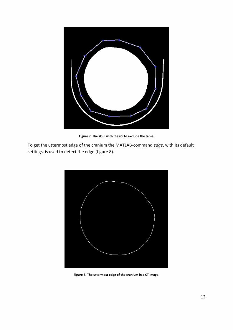
12

Figure 7. The skull with the roi to exclude the table.

To get the uttermost edge of the cranium the MATLAB-command edge, with its default

settings, is used to detect the edge (figure 8).

Figure 8. The uttermost edge of the cranium in a CT image.

13

3.2 Cephalometry images The cephalometry images are originally analogous images that have been digitalized by

taking pictures of them with a digital camera. The images are resized with a scale factor from

size M x N to size 400 x (N scale factor). The value of the scale factor depends on M. The

image needs to be resized because the original matrix is too large for the memory on the

computer.

3.2.1 Contrast enhancement In many of the cephalometry images there are very small differences in the intensity values

between the cranium and the background. The MATLAB-command adapthisteq, using its

default settings, enhances the contrast in the image by performing local histogram

equalization.

3.2.2 Definition of center-point, end-point, and unfused side Definition of center-point, end-point, and unfused side are performed in the same way as in

section 3.1.1.

3.2.3 Interactive definition of the cranium The cranium cannot be segmented automatically by the program due to poor contrast.

Therefore, it has to be done by hand. By clicking along the edge of the cranium points are

created, and its coordinates are saved in a vector. A MATLAB-command for creating lines is

recalling the vector and creating lines between the locations where the points are. The

points cannot be placed further apart than eight pixels, if they are, the program deletes the

latest point and the user has to click closer to the previous point.

3.3 Dividing the skull into two parts, one left and one right The coordinates from the defined center-point are used to divide the skull into two parts,

one left and one right side. The two parts are handled as two images. The unfused side is

also cropped at the point that defines how much of the skull that is of interest for the

comparison, the end-point (figure 9).

14

Figure 9. The segmented skull is divided into two parts, the fused side (left) and the unfused side (right). The unfused side is cropped at the end-point.

The image containing the left part is mirrored in a left-right direction, about a vertical axis.

To be able to perform the calculations the starting point of the two curves representing the

uttermost edge of the cranium, has to start in the middle of the matrix. The matrices should

also have the same size. This is done by adding matrices of zeros so that the output images

have the same size and the starting point is in the center of the matrix. The output matrix

contains the input image H and the matrices I and J (figure 10). I and J are zero matrices

where J has the same size as H, and I is of the size d x c. c is determined by calculating a-b.

The distances b and a are calculated by finding the coordinates of o in the input image H.

Figure 10. Schematic image of how zero matrices are added to get the center-point, o, in the middle. H is the input matrix, and I and J are matrices of zeros.

15

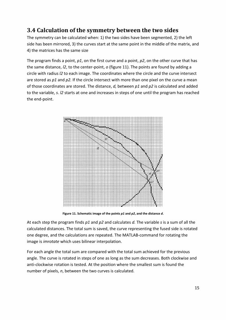
3.4 Calculation of the symmetry between the two sides The symmetry can be calculated when: 1) the two sides have been segmented, 2) the left

side has been mirrored, 3) the curves start at the same point in the middle of the matrix, and

4) the matrices has the same size

The program finds a point, p1, on the first curve and a point, p2, on the other curve that has

the same distance, l2, to the center-point, o (figure 11). The points are found by adding a

circle with radius l2 to each image. The coordinates where the circle and the curve intersect

are stored as p1 and p2. If the circle intersect with more than one pixel on the curve a mean

of those coordinates are stored. The distance, d, between p1 and p2 is calculated and added

to the variable, s. l2 starts at one and increases in steps of one until the program has reached

the end-point.

Figure 11. Schematic image of the points p1 and p2, and the distance d.

At each step the program finds p1 and p2 and calculates d. The variable s is a sum of all the

calculated distances. The total sum is saved, the curve representing the fused side is rotated

one degree, and the calculations are repeated. The MATLAB-command for rotating the

image is imrotate which uses bilinear interpolation.

For each angle the total sum are compared with the total sum achieved for the previous

angle. The curve is rotated in steps of one as long as the sum decreases. Both clockwise and

anti-clockwise rotation is tested. At the position where the smallest sum is found the

number of pixels, n, between the two curves is calculated.

16

If the left and the right side of the forehead are symmetrical n will be zero. The more

unsymmetrical the sides are the bigger the value is. The value does not only depend on the

symmetry but also the size of the head and the size of the pixels. To be able to compare the

symmetry this value has to be independent of these two components. It is therefore divided

by the number of pixels in the area denoted K which also depends on the size of the head

and the size of the pixels (figure 12). The normalized value is called the symmetry ratio, N. N

is multiplied with 1000 so that the numbers won’t be so small (equation 2).

(2)

Two methods, relative change (equation 3) and absolute change (equation 4), was tested as

an evaluation of how well the surgical operation has succeeded.

(3)

Figure 12. The gray area represent the area K .The area K is expressed in pixels and is used to normalize the result. The point p has the same distance, l2, to the center-point, o, as the end-point.

17

is the symmetry ratio for the pre-operative image, and is the symmetry

ratio for the post-operative image for the same patient. The closer C gets to one the better

the operation has succeeded. C can also have a negative value which shows that the

forehead is more asymmetrical after the operation.

(4)

The bigger B is the better the operation has succeeded. As for C, a negative value shows that

the forehead is more asymmetrical after the operation.

The MATLAB code is found in appendix I and a user manual is found in appendix II.

3.5 Evaluation of the program The program has been run several times to evaluate the program and see how reliable the

results are.

3.5.1 Symmetry evaluation The main aim for the program is to calculate the symmetry of the left and the right side of

the forehead. It should give a lower value for a more symmetrical forehead. The symmetry

ratio, N, was calculated for two images where it can be seen that one of the foreheads is

more symmetrical than the other (figure 13). The center- and end-point was placed at the

same structures in both images.

Figure 13. Two images where it can be seen that the forehead in the left image is more asymmetrical than the forehead in the right image.

18

3.5.2 Test on symmetrical phantoms A few tests was performed on a CT image of a cylindrical phantom to see if the result is zero

when the two sides are symmetrical, and if the result is independent of the rotation of the

head when the image is taken (figure 14). The symmetry ratio for this image was calculated

ten times. At every run the center-point and the end-point was placed on different places

along the uttermost edge of the circle to simulate that the head is rotated.

Figure 14. The cylindrical phantom.

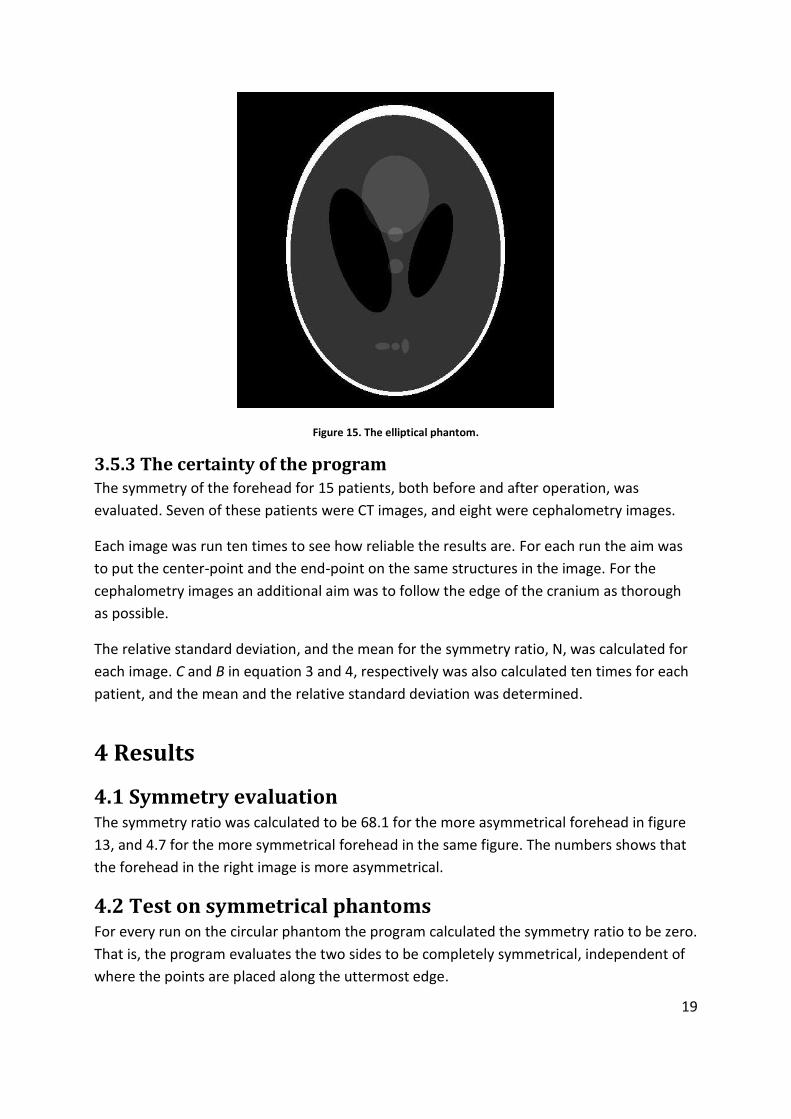
The program was also tested on an image of a symmetrical elliptical phantom (figure 15).

The image was created with the command phantom(512) in MATLAB. The image of the

phantom was run through the program twenty times. The aim for the first ten runs was to

place the center-point and the end-point at the same points on the uttermost edge of the

cranium. The aim for the last ten runs was to place the center-point at the same place for

each run and vary the places where the end-point was placed.

19

Figure 15. The elliptical phantom.

3.5.3 The certainty of the program The symmetry of the forehead for 15 patients, both before and after operation, was

evaluated. Seven of these patients were CT images, and eight were cephalometry images.

Each image was run ten times to see how reliable the results are. For each run the aim was

to put the center-point and the end-point on the same structures in the image. For the

cephalometry images an additional aim was to follow the edge of the cranium as thorough

as possible.

The relative standard deviation, and the mean for the symmetry ratio, N, was calculated for

each image. C and B in equation 3 and 4, respectively was also calculated ten times for each

patient, and the mean and the relative standard deviation was determined.

4 Results

4.1 Symmetry evaluation The symmetry ratio was calculated to be 68.1 for the more asymmetrical forehead in figure

13, and 4.7 for the more symmetrical forehead in the same figure. The numbers shows that

the forehead in the right image is more asymmetrical.

4.2 Test on symmetrical phantoms For every run on the circular phantom the program calculated the symmetry ratio to be zero.

That is, the program evaluates the two sides to be completely symmetrical, independent of

where the points are placed along the uttermost edge.

20

For all twenty runs on the elliptical phantom the program calculated the symmetry ratio to

be zero which means that the program evaluates the phantom to be completely

symmetrical.

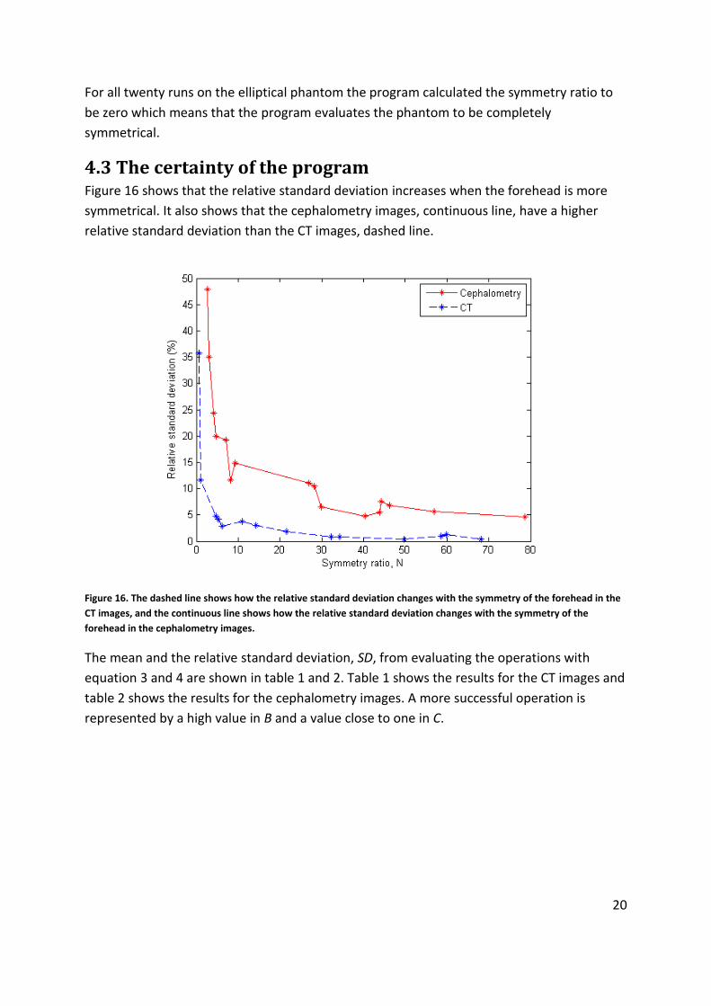
4.3 The certainty of the program Figure 16 shows that the relative standard deviation increases when the forehead is more

symmetrical. It also shows that the cephalometry images, continuous line, have a higher

relative standard deviation than the CT images, dashed line.

Figure 16. The dashed line shows how the relative standard deviation changes with the symmetry of the forehead in the

CT images, and the continuous line shows how the relative standard deviation changes with the symmetry of the

forehead in the cephalometry images.

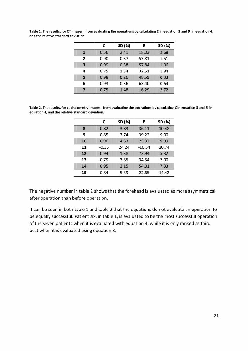
The mean and the relative standard deviation, SD, from evaluating the operations with

equation 3 and 4 are shown in table 1 and 2. Table 1 shows the results for the CT images and

table 2 shows the results for the cephalometry images. A more successful operation is

represented by a high value in B and a value close to one in C.

21

Table 1. The results, for CT images, from evaluating the operations by calculating C in equation 3 and B in equation 4, and the relative standard deviation.

C SD (%) B SD (%)

1 0.56 2.41 18.03 2.68

2 0.90 0.37 53.81 1.51

3 0.99 0.38 57.84 1.06

4 0.75 1.34 32.51 1.84

5 0.98 0.26 48.59 0.33

6 0.93 0.36 63.40 0.64

7 0.75 1.48 16.29 2.72

Table 2. The results, for cephalometry images, from evaluating the operations by calculating C in equation 3 and B in equation 4, and the relative standard deviation.

C SD (%) B SD (%)

8 0.82 3.83 36.11 10.48

9 0.85 3.74 39.22 9.00

10 0.90 4.63 25.37 9.99

11 -0.36 24.24 -10.54 20.74

12 0.94 1.38 73.94 5.32

13 0.79 3.85 34.54 7.00

14 0.95 2.15 54.01 7.33

15 0.84 5.39 22.65 14.42

The negative number in table 2 shows that the forehead is evaluated as more asymmetrical

after operation than before operation.

It can be seen in both table 1 and table 2 that the equations do not evaluate an operation to

be equally successful. Patient six, in table 1, is evaluated to be the most successful operation

of the seven patients when it is evaluated with equation 4, while it is only ranked as third

best when it is evaluated using equation 3.

22

5 Discussion Today the result of a surgical operation on a patient with unicoronal synostosis is evaluated

by studying the patient’s skull and at the x-ray images of the patient. There are no clear

criteria on how to evaluate the result. No clear criteria give an evaluation that is dependent

of the evaluator. Therefore, a program has been created as a quantitative measure to

evaluate the symmetry of the forehead in CT and cephalometry images of these patients,

and in the end to evaluate the result of the operation. The reliability of the program has

been tested on images of symmetrical phantoms and images of 15 patients before and after

the operation.

The poor contrast in some of the cephalometry images has caused some problems in

automatically detecting the uttermost edge of the cranium. In the end the solution to this

problem was to do this step manually. How the points are placed depends on the user and

will affect the result. If the time hadn’t been limited it might have been possible to come up

with a method that enhances the contrast in each image separately. This is an area which

can be further developed to improve the program. Although, in some images the contrast is

so poor that no enhancement technique would make it possible to segment the uttermost

edge. Even if the contrast could have been enhanced so that the edge could be segmented

automatically some of the pictures are in a way that the jaw is seen outside of the uttermost

edge of the cranium. The edge detected in an image like that would not be the uttermost

edge of the cranium but the jaw. If the program is developed to enhance the contrast in

each image separately, the problem with the jaw might be overcome by a combination of

automatically and manually segmentation of the edge.

As can be seen in figure 16 the relative standard deviation increase when the symmetry ratio

decrease. If the center-point and the end-point aren’t placed at exactly the same place every

time, the number of pixels between the curves representing the uttermost edge of the

cranium will vary. If the curves are more symmetrical the number of pixels between them

will be lower and this variation will have a higher impact on the result. Figure 16 also shows

that the uncertainty for the cephalometry images is considerably higher and varies more

than the uncertainty for the CT images.

As mentioned, the relative standard deviation increases when the symmetry ratio decreases.

The curve representing the cephalometry images in figure 16 shows that this is not always

the case. Although, it can be seen that despite that the values differ from what might have

been expected the variation is only a few percent, and an increase of the standard deviation

at lower values on the symmetry ratio can be distinguished. These variations can depend on

tree things; 1) there are some distinct structures where the center-point and the end-point is

placed which makes it easier to place the points at exactly the same point every time, 2) the

edge isn’t defined as thorough for each run, and 3) if there are big changes in the curves

appearances around the center-point and the end-point a variation in the placement of

23

these points will affect the result more than if the curves is more constant around the

points.

Number one and number three in the previous section might also be a reason for the

variations shown in the results for the CT-images in figure 16.

If the skull is completely symmetrical the place where the end-point is placed is less

important than the place where the center-point is placed. In that case, if the center-point is

placed in a way that the forehead is divided into two completely symmetrical parts the

placement of the end-point won’t affect the result at all. This is shown by the results from

the test on the elliptical phantom where it is calculated that the two sides are completely

symmetrical, even if the end-point is placed at different places each time.

As mentioned in the result, the two evaluation methods presented in equation 3 and 4 do

not evaluate an operation to be equally successful. An operation evaluated to be successful

by one of the equations might be evaluated to be less successful by the other. It would have

been interesting to compare the results with previous clinical evaluations but no such

evaluations have been done before. If the symmetry ratio is calculated to be 70 before

operation and 40 after operation, equation 4 evaluates the operation to be more successful

than if the symmetry ratio is calculated to be 20 before operation and 0 after operation,

even if the last operation is as successful as it can be. Equation 3 on the other hand would

evaluate the last operation to be more successful than the first. By dividing the difference

between the symmetry ratio before operation and after operation with the symmetry ratio

before operation the result will show the relative change. The relative change allows the

results for different patients to be compared even if the symmetry ratio before operation

differs between the patients. If equation 4 is used an operation where the symmetry ratio

before operation is high will be evaluated as a more successful operation. It seems that

equation 3 is preferable for evaluation of clinical materiel, since it has an upper limit of

success, i. e. C=1 means perfect operation, and C=0 means no difference, and C less than

zero means that the forehead is more asymmetrical after the surgery. As discussed above

equation 4 do not give this information in a clear way.

In the evaluation of patient 11 in table 2, it is shown that the forehead is more asymmetrical

after operation than before operation. The surgical operation has not succeeded; in fact it

has worsened the symmetry of the forehead. This is shown, as discussed in the previous

section, as a negative value in both evaluation methods. Both methods show a pretty low

difference. Therefore, small variations between each run will affect the result more which is

shown by the high relative standard deviation.

As can be seen in figure 16 the relative standard deviation is relatively high for a low value of

the symmetry ratio. When the absolute or the relative change is calculated the result is

24

dominated by the higher symmetry ratio, resulting in a relatively low relative standard

deviation.

An attempt has been made to increase the size of the image, not the matrix, so that the

edge can be distinguished more easily when it is defined manually. When this is done

something goes wrong and some parts of the edge are lost. The reason for that has not been

established.

Another thing that can be further developed in the program is the processing time. At the

time, one image takes approximately ten minutes, which might be a problem for longer

patient series. Therefore, future studies should focus on optimizing the present MATLAB

code.

25

6 Conclusions A MATLAB tool to evaluate the symmetry of the forehead in patients with unicoronal

synostosis before and after treatment has been developed for both CT and cephalometry

images which was the main aim of this project. The method is also independent of the heads

rotation at the time when the image is taken. It is shown that the results are more reliable

when CT images are evaluated than when cephalometry images are evaluated. The

recommendation for evaluating an operation is to calculate the relative change.

26

Acknowledgements I would like to take the opportunity to thank everyone who has helped me to complete this

project. First of all I would like to thank my supervisors Peter Bernhard at the Department of

Radiation Physics, and Lars Kölby at the craniofacial unit at the Department of Plastic

Surgery, for their guidance and quick answers to my endless questions. Also a big thank you

to my supervisor Jacob Heydorn-Lagerlöf at the Department of Radiation Physics for all his

help with MATLAB, and for his guidance through everything that this computing tool has to

offer.

Thanks to Patrik Sund at the Department of Radiation Physics, and Giovanni Maltese at the

craniofacial unit at the Department of Plastic Surgery for all their help along the way.

Finally, special thanks to my classmates, friends and family who has helped me, in their own

special ways, to end this project as well as pass my studies.

27

References 1. Jane, J.A. and M.S. McKisic. Craniosynostosis. Apr 2, 2010 [cited 2010 Nov 2]; Available from:

http://emedicine.medscape.com/article/248568-overview. 2. Podda, S., et al. Craniosynostosis Management. sep 17, 2008 [cited 2010 oct 21]; Available

from: http://emedicine.medscape.com/article/1281182-overview. 3. Boulet, S.L., S.A. Rasmussen, and M.A. Honein, A population-based study of craniosynostosis

in metropolitan Atlanta, 1989-2003. Am J Med Genet A, 2008. 146A(8): p. 984-991. 4. Hayward, R., The clinical management of craniosynostosis. Clinics in developmental

medicine, 0069-4835; 163. 2004, London: Cambridge UP. 5. Wikipedia, Coronal suture. 6. Gonzalez, R.C. and R.E. Woods, Digital image processing. 2008, Upper Saddle River, N.J.:

Pearson Prentice Hall. 7. MathWorks. MATLAB. [cited 2010 Nov 19]; Available from:

http://www.mathworks.com/products/matlab/description1.html.

8. MathWorks. Functional design clunkers. [cited 2010 nov 25]; Available from: http://blogs.mathworks.com/steve/2009/08/31/functional-design-clunkers/.

28

Appendix

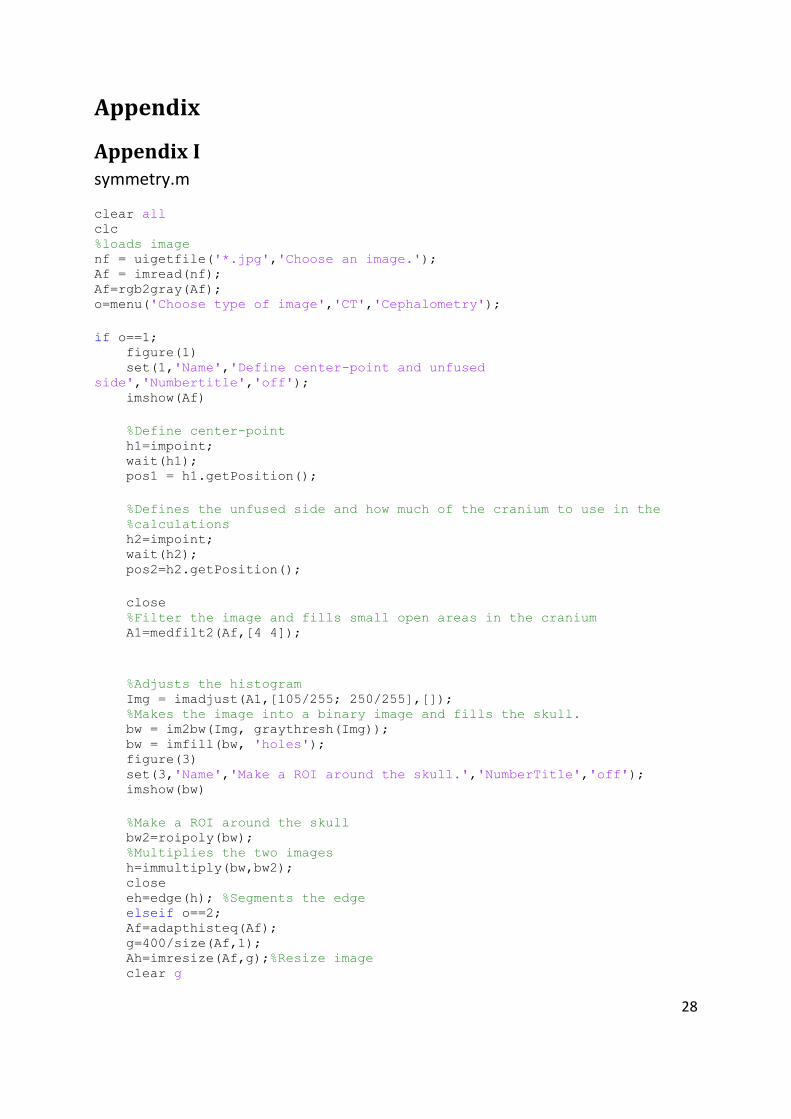
Appendix I symmetry.m

clear all clc %loads image nf = uigetfile('*.jpg','Choose an image.'); Af = imread(nf); Af=rgb2gray(Af); o=menu('Choose type of image','CT','Cephalometry');

if o==1; figure(1) set(1,'Name','Define center-point and unfused

side','Numbertitle','off'); imshow(Af)

%Define center-point h1=impoint; wait(h1); pos1 = h1.getPosition();

%Defines the unfused side and how much of the cranium to use in the %calculations h2=impoint; wait(h2); pos2=h2.getPosition();

close %Filter the image and fills small open areas in the cranium A1=medfilt2(Af,[4 4]);

%Adjusts the histogram Img = imadjust(A1,[105/255; 250/255],[]); %Makes the image into a binary image and fills the skull. bw = im2bw(Img, graythresh(Img)); bw = imfill(bw, 'holes'); figure(3) set(3,'Name','Make a ROI around the skull.','NumberTitle','off'); imshow(bw)

%Make a ROI around the skull bw2=roipoly(bw); %Multiplies the two images h=immultiply(bw,bw2); close eh=edge(h); %Segments the edge elseif o==2; Af=adapthisteq(Af); g=400/size(Af,1); Ah=imresize(Af,g);%Resize image clear g

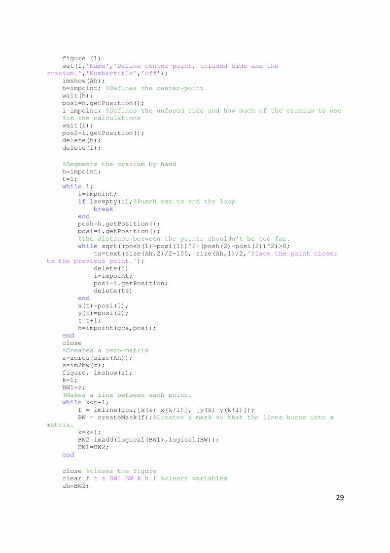
29

figure (1) set(1,'Name','Define center-point, unfused side and the

cranium.','Numbertitle','off'); imshow(Ah); h=impoint; %Defines the center-point wait(h); pos1=h.getPosition(); i=impoint; %Defines the unfused side and how much of the cranium to use %in the calculations wait(i); pos2=i.getPosition(); delete(h); delete(i);

%Segments the cranium by hand h=impoint; t=1; while 1; i=impoint; if isempty(i);%Pusch esc to end the loop break end posh=h.getPosition(); posi=i.getPosition(); %The distance between the points shouldn't be too far. while sqrt((posh(1)-posi(1))^2+(posh(2)-posi(2))^2)>8; ts=text(size(Ah,2)/2-100, size(Ah,1)/2,'Place the point closer

to the previous point.'); delete(i) i=impoint; posi=i.getPosition; delete(ts) end x(t)=posi(1); y(t)=posi(2); t=t+1; h=impoint(gca,posi); end close %Creates a zero-matrix z=zeros(size(Ah)); z=im2bw(z); figure, imshow(z); k=1; BW1=z; %Makes a line between each point. while k<t-1; f = imline(gca,[x(k) x(k+1)], [y(k) y(k+1)]); BW = createMask(f);%Creates a mask so that the lines burns into a

matrix. k=k+1; BW2=imadd(logical(BW1),logical(BW)); BW1=BW2; end

close %closes the figure clear f t z BW1 BW k h i %clears variables eh=BW2;

30

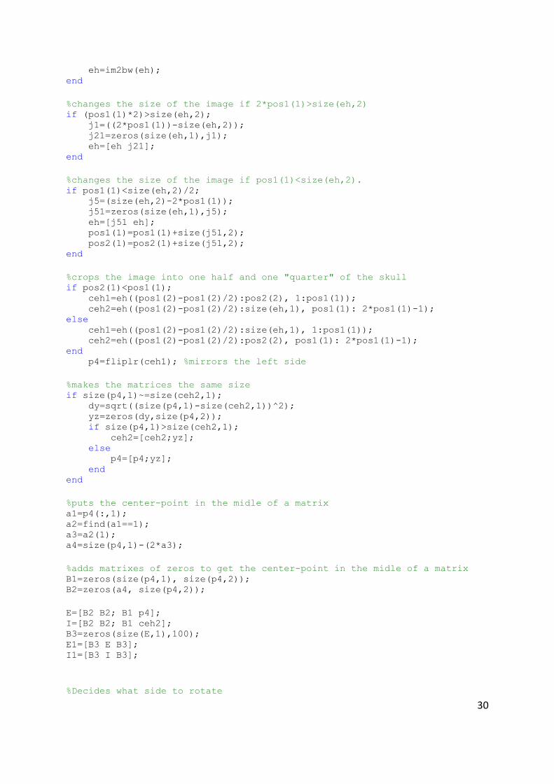
eh=im2bw(eh); end

%changes the size of the image if 2*pos1(1)>size(eh,2) if (pos1(1)*2)>size(eh,2); j1=((2*pos1(1))-size(eh,2)); j21=zeros(size(eh,1),j1); eh=[eh j21]; end

%changes the size of the image if pos1(1)<size(eh,2). if pos1(1)<size(eh,2)/2; j5=(size(eh,2)-2*pos1(1)); j51=zeros(size(eh,1),j5); eh=[j51 eh]; pos1(1)=pos1(1)+size(j51,2); pos2(1)=pos2(1)+size(j51,2); end

%crops the image into one half and one "quarter" of the skull if pos2(1)<pos1(1); ceh1=eh((pos1(2)-pos1(2)/2):pos2(2), 1:pos1(1)); ceh2=eh((pos1(2)-pos1(2)/2):size(eh,1), pos1(1): 2*pos1(1)-1); else ceh1=eh((pos1(2)-pos1(2)/2):size(eh,1), 1:pos1(1)); ceh2=eh((pos1(2)-pos1(2)/2):pos2(2), pos1(1): 2*pos1(1)-1); end p4=fliplr(ceh1); %mirrors the left side

%makes the matrices the same size if size(p4,1)~=size(ceh2,1); dy=sqrt((size(p4,1)-size(ceh2,1))^2); yz=zeros(dy,size(p4,2)); if size(p4,1)>size(ceh2,1); ceh2=[ceh2;yz]; else p4=[p4;yz]; end end

%puts the center-point in the midle of a matrix a1=p4(:,1); a2=find(a1==1); a3=a2(1); a4=size(p4,1)-(2*a3);

%adds matrixes of zeros to get the center-point in the midle of a matrix B1=zeros(size(p4,1), size(p4,2)); B2=zeros(a4, size(p4,2));

E=[B2 B2; B1 p4]; I=[B2 B2; B1 ceh2]; B3=zeros(size(E,1),100); E1=[B3 E B3]; I1=[B3 I B3];

%Decides what side to rotate

31

if pos2(1)<pos1(1); Ik=I1; E3=E1; b=1; else E3=I1; Ik=E1; b=0; end

s1=0; s2=0; v=0; j2=0; f=0.24; while s1<=s2; I3=imrotate(Ik,v,'bilinear','crop'); I3(find(I3>f))=1; I3=im2bw(I3); s2=s1; %Store the latest value of s1 in s2 s1=0; t=size(E1,1)/2+1; l2=1;

while t<=size(E1,1); %Runs the while-loop until the line in E3 ends. %Makes a cirkle with radius l2 T=zeros(size(E1)); T2=T; x0=size(T,2)/2; y0=size(T,1)/2;

for i=1:size(T,2); for j=1:size(T,1); r=sqrt((i-x0)^2+(j-y0)^2); T(j,i)=r; end end L=find(T<=l2); T2(L)=1; L1=edge(T2); L1=medfilt2(L1,[1 2]); %widens the edge of the circle so that the % circle won't mis the curve even if the curve hasn't ended. L2=immultiply(L1,I3); %Finds a point in I3 that has the same radii %as a point in E3. L3=immultiply(L1,E3); %Finds a point in E3 that has the same radii %as a point in I3 [row, col]=find(L2); %Finds the coordinates of every pixels with %value one [row1, col1]=find(L3); %Finds the coordinates of every pixels with %value one if isempty(row1)|| isempty(row);%Breaks the loop when it reaches

the %end of the curve representing the unfused side break end R=L1; %finds the points where the curves and the circle intersect x1=mean(col1); x2=mean(col);

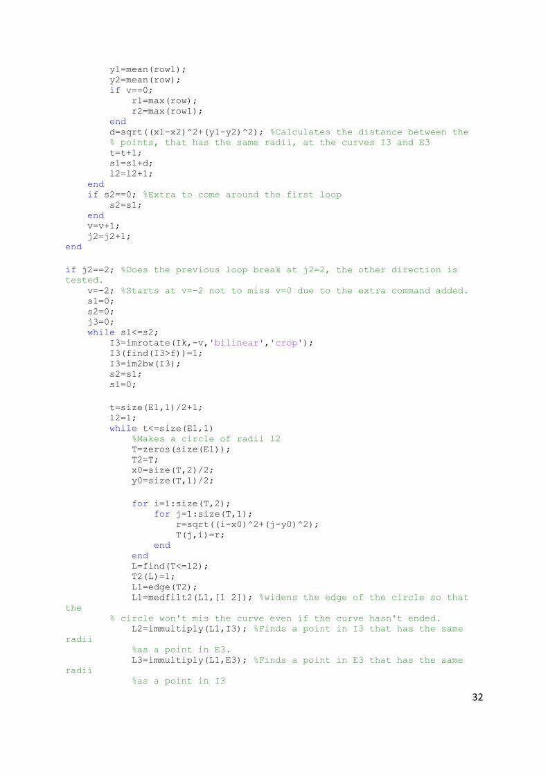
32

y1=mean(row1); y2=mean(row); if v==0; r1=max(row); r2=max(row1); end d=sqrt((x1-x2)^2+(y1-y2)^2); %Calculates the distance between the % points, that has the same radii, at the curves I3 and E3 t=t+1; s1=s1+d; l2=l2+1; end if s2==0; %Extra to come around the first loop s2=s1; end v=v+1; j2=j2+1; end

if j2==2; %Does the previous loop break at j2=2, the other direction is

tested. v=-2; %Starts at v=-2 not to miss v=0 due to the extra command added. s1=0; s2=0; j3=0; while s1<=s2; I3=imrotate(Ik,-v,'bilinear','crop'); I3(find(I3>f))=1; I3=im2bw(I3); s2=s1; s1=0;

t=size(E1,1)/2+1; l2=1; while t<=size(E1,1) %Makes a circle of radii l2 T=zeros(size(E1)); T2=T; x0=size(T,2)/2; y0=size(T,1)/2;

for i=1:size(T,2); for j=1:size(T,1); r=sqrt((i-x0)^2+(j-y0)^2); T(j,i)=r; end end L=find(T<=l2); T2(L)=1; L1=edge(T2); L1=medfilt2(L1,[1 2]); %widens the edge of the circle so that

the % circle won't mis the curve even if the curve hasn't ended. L2=immultiply(L1,I3); %Finds a point in I3 that has the same

radii %as a point in E3. L3=immultiply(L1,E3); %Finds a point in E3 that has the same

radii %as a point in I3

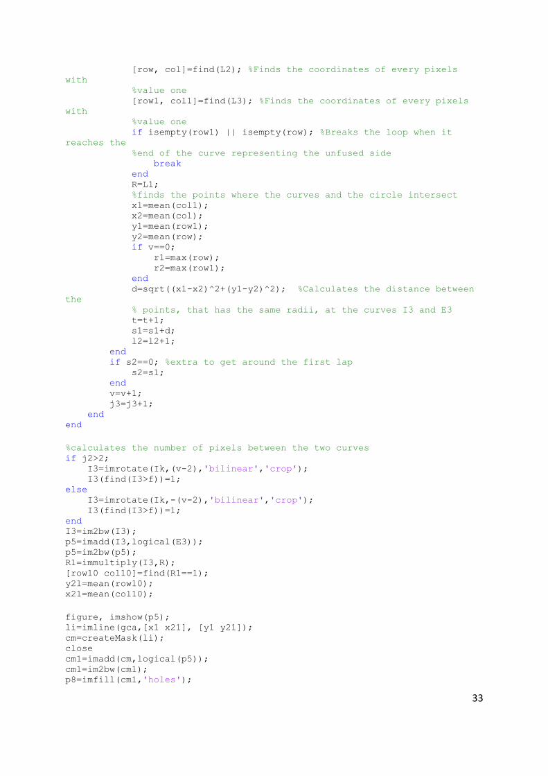
33

[row, col]=find(L2); %Finds the coordinates of every pixels

with %value one [row1, col1]=find(L3); %Finds the coordinates of every pixels

with %value one if isempty(row1) || isempty(row); %Breaks the loop when it

reaches the %end of the curve representing the unfused side break end R=L1; %finds the points where the curves and the circle intersect x1=mean(col1); x2=mean(col); y1=mean(row1); y2=mean(row); if v==0; r1=max(row); r2=max(row1); end d=sqrt((x1-x2)^2+(y1-y2)^2); %Calculates the distance between

the % points, that has the same radii, at the curves I3 and E3 t=t+1; s1=s1+d; l2=l2+1; end if s2==0; %extra to get around the first lap s2=s1; end v=v+1; j3=j3+1; end end

%calculates the number of pixels between the two curves if j2>2; I3=imrotate(Ik,(v-2),'bilinear','crop'); I3(find(I3>f))=1; else I3=imrotate(Ik,-(v-2),'bilinear','crop'); I3(find(I3>f))=1; end I3=im2bw(I3); p5=imadd(I3,logical(E3)); p5=im2bw(p5); R1=immultiply(I3,R); [row10 col10]=find(R1==1); y21=mean(row10); x21=mean(col10);

figure, imshow(p5); li=imline(gca,[x1 x21], [y1 y21]); cm=createMask(li); close cm1=imadd(cm,logical(p5)); cm1=im2bw(cm1); p8=imfill(cm1,'holes');

34

p9=imsubtract(p8,p5); n1=find(p9==1); n3=length(n1);%the number of pixels between the two curves

%calculates the number of pixels in the area denoted K N=fliplr(E1); if b==1; f3=N(r2,:); col4=find(f3==1); z3=col4(1); f4=I1(r1,:); col5=find(f4==1); z4=col5(1); else f3=I1(r2,:); col4=find(f3==1); z3=col4(1); f4=N(r1,:); col5=find(f4==1); z4=col5(1); end

N4=imadd(N,I1); g=imline(gca,[z3 z4], [r2 r1]); bw1 = createMask(g); close k=imadd(bw1,logical(N4)); k1=imfill(k,'holes'); k2=imsubtract(k1,k); figure, imshow(k2); n=find(k2==1); n2=length(n); %number of pixels in the area K

sum2=round(n3/n2*1000);%the symmetry ratio is calculated and multiplied %with 1000 so that the numbers won't be so small. sum=num2str(sum2); resultatruta(sum)

35

Appendix II User manual.

Install program

1. Run Symmetry_pkg.

2. Run the program Symmetry.

Run program

1. Choose an image (it is important that the image is in the same folder as the program). Verify what type of image it is. 1.1. CT

1.1.1. Define the center-point and how much of the cranium the program should use

when doing the calculations, this point is placed on the unfused side. Using the

mouse, you select the points by left-clicking. The point can be moved until you

verify the location by double-clicking on the point.

1.1.2. Place a ROI around the skull. Using the mouse, you specify the region by

selecting vertices around the skull by left-clicking. To close the ROI move the

pointer over the initial vertex of the polygon that you selected. The pointer

changes to a circle. Click either mouse button. You can move or resize the ROI

using the mouse. When you are finished positioning and sizing the ROI, double-

clicking or right-clicking inside the region will start the calculations.

1.2. Cephalometry

1.2.1. Define the center-point and how much of the cranium the program should use

when doing the calculations, this point is placed on the unfused side. Using the

mouse, you select the points by left-clicking. The point can be moved until you

verify the location by double-clicking on the point. Also define the cranium by

interactive placement of points along the whole edge of the cranium. Once the

point is placed it cannot be moved. When the cranium is defined push esc to

proceed.