maximenko and jan

SCUD☺: Surface CUrrents from Diagnostic model

Nikolai Maximenko and Jan Hafner

IPRC Technical Note No. 5

February 16, 2010

☺ The Free Dictionary (http://www.thefreedictionary.com) to scud - to move along swiftly and smoothly Examples: ‐ clouds scudding the sky ‐ drifters scudding the ocean We do not know what velocity do drifters measure, but we do know that they measure it accurately, thus providing a kind of reference. The SCUD product extends this reference to times when and locations where drifters are not there. Table of Content

page

1. Purpose and ideas of the SCUD dataset.................................... 1 2. Data used to produce the SCUD............................................... 1

2.1 AVISO sea level anomaly 2.2 Mean Dynamic Ocean Topography (MDOT) 2.3 QuikSCAT wind 2.4 Drifter trajectories

3. Technique..................................................................................2 3.1 Interpolation on to drifter locations 3.2 Low‐pass filtering 3.3 Linear regression

4. SCUD coefficients.......................................................................4 5. Fit to data...................................................................................9 6. Statistics of SCUD velocity..........................................................10 7. Access to SCUD data..................................................................14 8. Copyright, terms of use, registration and feedback....................16 9. Acknowledgments....................................................................17 10. References...............................................................................17

1. Purpose and ideas of the SCUD dataset

Ocean currents are one of the variables that are most difficult for observations, both in situ and remote. Only satellites can provide global coverage continuous in time. Previous efforts were based on assumptions of geostrophy (AVISO), linear ageostrophic response to local wind (Uchida and Imawaki, 2003), and/or simple models of the mixed layer (Bonjean and Lagerloef, 2002).

SCUD also assumes that total surface velocity is comprised of the component linear to the local horizontal pressure gradient (but not necessarily geostrophic balance) and the component linear to the local surface wind (but not necessarily Ekman‐kind balance).

SCUD coefficients are tuned to best reproduced velocities derived from trajectories of standard drifters drogued at 15 meters depth. Nominally, the drifters average horizontal velocity between 12 and 18 meters. Actual meaning of the SCUD data may differ due to complex dynamics of the drifters. The dataset aims the tasks of diagnosing trajectories of a tracer floating at or near the sea surface, such as marine debris, oil spills, etc. Movement of particular kind of the tracer may systematically differ from the one of the standard drifters used in the SCUD model.

While the SCUD is designed to provide nearly global, daily velocities, the user is strongly advised to carefully read this manual and to bear in mind limitations of the dataset based on multiple assumptions described in the following sections.

2. Data used to produce the SCUD

2.1 AVISO sea level anomaly AVISO sea level anomaly was used in the determination of the geostrophic current components. Mercator‐gridded 1/3° delayed time product DT‐MSLA "Upd" was selected and the data were acquired from the AVISO data server (ftp://ftp.aviso.oceanobs.com/pub/oceano/AVISO/SSH/duacs/global/dt/upd/msla/merged/h/). This is a merged product based on all available satellites (up to 4 at some times) with improved sampling and long‐wave error determination. Prior to use in SCUD, the sea level anomaly was corrected to account for different time spans used for definitions of sea level 'anomaly' (1992‐1999) and 'mean' dynamic topography (1992‐2002).

2.2 Mean Dynamic Ocean Topography (MDOT) MDOT used in SCUD was produced by Maximenko et al. (2009), who combined drifter, satellite altimetry, surface winds, and GRACE data to derive the mean ocean surface topography for the period 1992 – 2002 on a 1/2° global grid. The MDOT data is available at apdrc.soest.hawaii.edu/datadoc/mdot.php and was used in SCUD to compute the mean geostrophic velocity.

2.3 QuikSCAT wind

QuikSCAT wind product data utilized in SCUD product were acquired from the Remote Sensing Systems (ssmi.com/qscat/qscat_description.html). The daily produced ¼° maps of zonal and meridional wind components were used. QuikSCAT data are available from 20 July 1999 through 19 November 2009 (when the satellite failed) and the latest product version is v03a.

1

ftp://ftp.aviso.oceanobs.com/pub/oceano/AVISO/SSH/duacs/global/dt/upd/msla/merged/h/

2.4 Drifter trajectories

Trajectories of 8058 drifters, drogued at 15 meters depth and covering time period from February 1979 through September 2008, were acquired from the NOAA Atlantic Oceanographic and Meteorological Laboratory (AOML) (www.aoml.noaa.gov/envids/gld/FtpInterpolatedInstructions.php), where drifter locations were quality‐controlled and objectively interpolated (krigged) on to every 6 hours. Drifters velocities, used in SCUD, were derived from drifter displacements over 12 hours.

3. Technique 3.1 Interpolation on to drifter locations

Components of the horizontal gradient of the AVISO sea level anomaly, horizontal gradient of MDOT, and QSCAT wind vectors were interpolated linearly in space and in time on to 6‐hourly locations and times of drifters. No extrapolation had been done, i.e. the interpolation was only performed where all eight grid points (four nearest points for each of the two nearest time layers) had data.

3.2 Low‐pass filtering To eliminate high‐frequency motions of drifters that are controlled by the physics that does not suggest signatures in sea level and wind data at scales provided by satellites, all concurrent data were filtered along drifter trajectories with the running Hanning (cosine) filter, having the half‐width equal to the local period of inertial oscillations, but not larger than 3 days. (3‐day inertial period is reached at latitude 9037'.)

3.3 Linear regression The SCUD velocity is assumed to be related to local instantaneous pressure gradient and wind as follows. USCUD (x,y,t) = U0 + uhx⋅∇xh(x,y,t) + uhy⋅ ∇yh(x,y,t) + uwx⋅wx(x,y,t) + uwy⋅wy (x,y,t), (1) VSCUD (x,y,t) = V0 + vhx⋅∇xh(x,y,t) + vhy⋅∇yh(x,y,t) + vwx⋅wx(x,y,t) + vwy⋅wy(x,y,t) , where U0, V0, uhx, vhx, uhy, vhy, uwx, vwx, uwy, vwy are the ten coefficients of the SCUD model. All coefficients are only functions of longitude and latitude and are independent of time. Different groups of the coefficients are expected to have different spatial scales. Under the geostrophic balance vhx and uhy vary on planetary scale and only depend on latitude while are uhx and vhy vanish. Correlation between drifter velocities and local winds is usually relatively low, and consistent assessment of the coefficients requires large datasets. Under the limited number of drifter data, this task can be solved in large domains, i.e. on a coarse grid. Fortunately, Ekman current are assumed to have the scale of atmospheric vortices (typically thousands of kilometers), and secondary circulation due to air‐sea coupling over ocean SST fronts is generally weak. Alternatively, U0 and V0 have the meaning of the mean surface velocities and are shown to contain important global system of strong, narrow geostrophic jets (e.g., Maximenko et al., 2009). To allow larger bins for the ‘wind’ coefficients uwx, vwx, uwy, vwy without over‐smoothing the 'mean' coefficients U0, V0, the latter were split on to smaller scale mean geostrophic velocities, known from the MDOT, and unknown larger‐scale ageostrophic component

2

U0 = u0 + Ug , V0 = v0 + Vg , (2) where Ug = ‐ g/fm⋅∂H/∂y, Vg = g/fm⋅∂H/∂x, (3) and fm(y) is the modified Coriolis parameter. This modification is to avoid singularity associated with geostrophic currents at the equator and is limited to the latitude band 100S to 100N, where 1/fm is set to be a linear function of latitude (Fig. 1). Currents near the equator, not included into Ug, Vg, are relatively broad and their reproduction by the model should not be significantly impacted by the use of larger bins.

Figure 1. Dependence of 1/fm on latitude, where fm is the modified Coriolis parameter.

The ten coefficients (u0, v0, uhx, vhx, uhy, vhy, uwx, vwx, uwy, vwy) are calculated by minimizing the costfunction F=Σ[(Ud ‐ USCUD)

2 + (Vd ‐ VSCUD)2] , (4)

where Σ denotes summation over all the concurrent data in the bin. The task is naturally reformulated in the form of system of ten linear equations. Bins are 3ox3o bins with the centers on 1ox1o. Only the bins where number of data exceeds 15 (out nearly 5,700,000 total 6‐hourly data used) are utilized in calculations, there are 31824 such bins globally. Each coefficient is then linearly interpolated on the QuikSCAT (1/4ox1/4o) grid and masked. The mask is defined manually based on data and land distributions (Fig. 2)

Figure 2. Areas (blue) covered with the SCUD velocities.

3

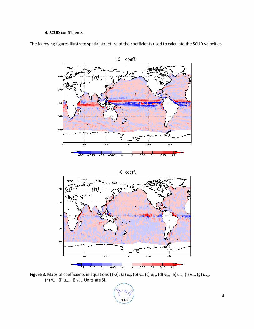
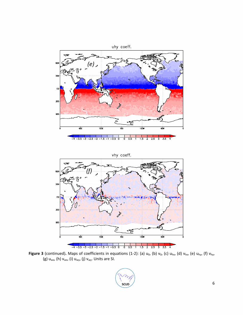
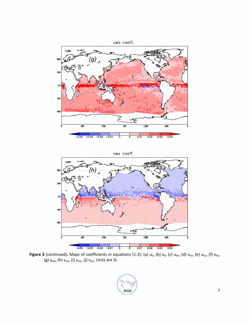
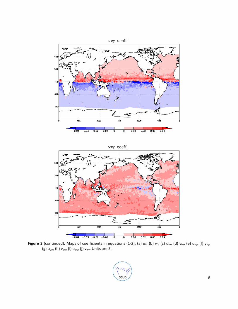
4. SCUD coefficients

The following figures illustrate spatial structure of the coefficients used to calculate the SCUD velocities.

(a)

(b)

Figure 3. Maps of coefficients in equations (1‐2): (a) u0, (b) v0, (c) uhx, (d) vhx, (e) uhy, (f) vhy, (g) uwx, (h) vwx, (i) uwy, (j) vwy. Units are SI.

4

(c)

(d)

Figure 3 (continued). Maps of coefficients in equations (1‐2): (a) u0, (b) v0, (c) uhx, (d) vhx, (e) uhy, (f) vhy, (g) uwx, (h) vwx, (i) uwy, (j) vwy. Units are SI.

5

(e)

(f)


6

(g)

(h)


7

(i)

(j)


8

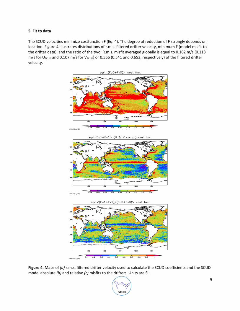
5. Fit to data

The SCUD velocities minimize costfunction F (Eq. 4). The degree of reduction of F strongly depends on location. Figure 4 illustrates distributions of r.m.s. filtered drifter velocity, minimum F (model misfit to the drifter data), and the ratio of the two. R.m.s. misfit averaged globally is equal to 0.162 m/s (0.118 m/s for USCUD and 0.107 m/s for VSCUD) or 0.566 (0.541 and 0.653, respectively) of the filtered drifter velocity.

(a)

(b)

(c)

Figure 4. Maps of (a) r.m.s. filtered drifter velocity used to calculate the SCUD coefficients and the SCUD model absolute (b) and relative (c) misfits to the drifters. Units are SI.

9

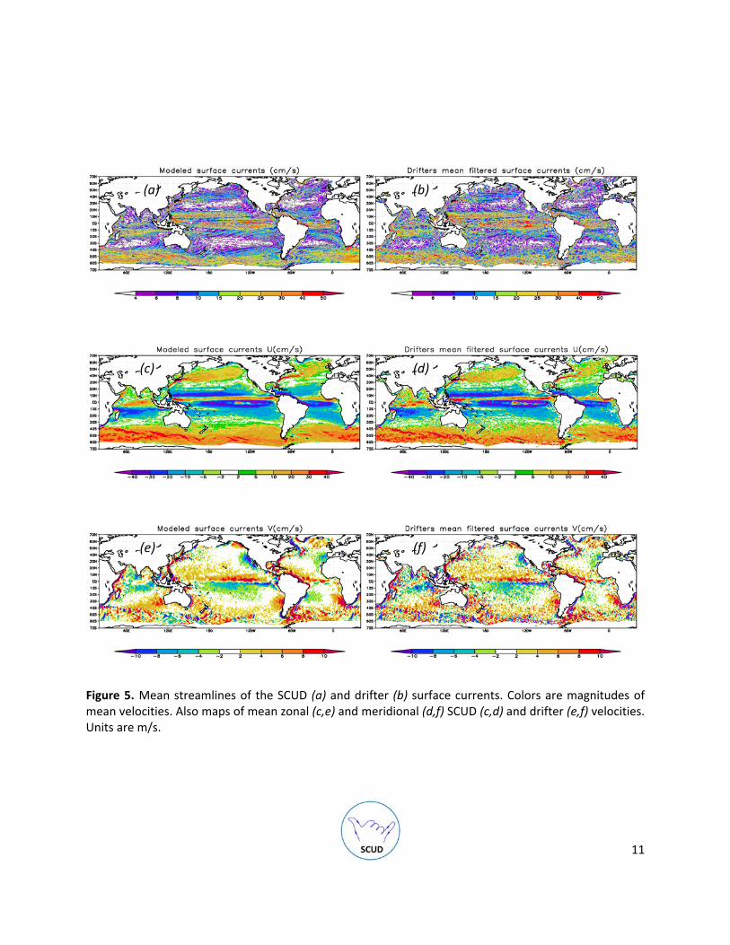
6. Statistics of SCUD velocity

Figures 5 illustrate good correspondence between the statistics of the SCUD and drifter velocities. Velocities associated with the sea level gradient are generally stronger than velocities induced by the wind (Figs. 7 and 9). The latter are however significant where geostrophic currents are weak (central and eastern parts of some subpolar and subtropical gyres) as well as on the equator and in the Southern Ocean. Even weaker ageostrophic velocities are fully responsible for horizontal convergences and divergences in the upper ocean, and instantaneous ageostrophic currents may be much stronger than time‐averaged ones. Equation (3) exemplifies currents in geostrophic balance with the horizontal gradient of sea level. In the ideal balance, uhx= 0, 1‐ f/g⋅vhx = 0, f/g⋅uhy +1 =0, and vhy= 0. (5) Figure 8 shows that actual balance is close to geostrophy in many areas in mid‐latitudes. At high latitudes (especially, in the North Pacific) and in tropics, deviation from geostrophy is consistent with the spatial oversmoothing of the altimeter data by the AVISO mapping technique. This is also supported by the generally larger deviation from the geostrophy in zonal sea level gradient (Fig. 8b), asessed from the difference between sparse tracks, than in meridional gradient (Fig. 8a), assessed from dense along‐track sampling. Coefficient uhx and vhy do not vanish near the equator (Figs. 3c, f). While vhy corresponds to currents against pressure gradient, usual in a non‐rotating system, uhx is more noisy and generally suggests currents down the pressure gradient. Additional bias from the geostrophy might occur in regions where effects of sea level and wind cannot be fully separated. Variance of model currents in Figure 6 is systematically lower than variance of drifter velocities. This may be because the SCUD model is oversimplified. E.g., coefficients assumed to be constant in time may actually be dependent on many factors. Classical Ekman response to local wind is isotropic in a sense that the angle and the coefficient between wind vector and Ekman velocity are only functions of depth and do not depend on the wind direction. This is not always true for the SCUD coefficients uwx, vwx, uwy, and vwy. Degree of anisotropy of the SCUD velocity response to the wind is illustrated by Figure 10, showing the map of [(uwx ‐ vwy)

2 + (uwy + vwx)2]/ [{(uwx + vwy)/2}

2 + {(uwy + vwx)/2}2] , (6)

characterizing relative departure of the matrix from a rotational one. The largest anisotropy is in tropics and in some coastal areas. While the exact source of the anisotropy is not known, likely candidates are interactions with baroclinic fronts, correlation between sea level and wind, alias between such control parameters as wind direction and strength, and others.

10

(a) (b)

(c) (d)

(e) (f)

Figure 5. Mean streamlines of the SCUD (a) and drifter (b) surface currents. Colors are magnitudes of mean velocities. Also maps of mean zonal (c,e) and meridional (d,f) SCUD (c,d) and drifter (e,f) velocities. Units are m/s.

11

(a) (b)

(c) (d)

Figure 6. Variances of the zonal (a, c) and meridional (b,d) SCUD (a,b) and drifter (c,d) velocities.

Figure 7. R.m.s SCUD velocity associated with variations of sea level. Units are m/s.

12

(a)

(b)

Figure 8. Degree of geostrophy of the zonal (a) and meridional (b) SCUD velocities.

13

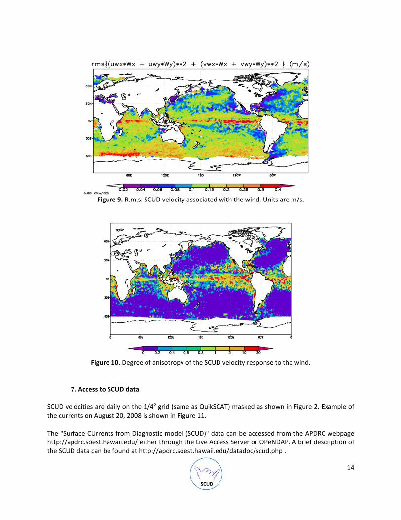
Figure 9. R.m.s. SCUD velocity associated with the wind. Units are m/s.

Figure 10. Degree of anisotropy of the SCUD velocity response to the wind.

7. Access to SCUD data

SCUD velocities are daily on the 1/4o grid (same as QuikSCAT) masked as shown in Figure 2. Example of the currents on August 20, 2008 is shown in Figure 11. The "Surface CUrrents from Diagnostic model (SCUD)" data can be accessed from the APDRC webpage http://apdrc.soest.hawaii.edu/ either through the Live Access Server or OPeNDAP. A brief description of the SCUD data can be found at http://apdrc.soest.hawaii.edu/datadoc/scud.php .

14

(a)

(b)

(c)

Figure 11. Streamlines (a) of the ('frozen') SCUD velocity on August 20, 2008. Colors are speed. Also maps of (b) zonal and (c) meridional velocity components on the same day. Units are cm/s.

15

8. Copyright, terms of use, registration, and feedback The SCUD dataset is open for free unrestricted use, copying and distribution. The dataset is a research quality product. Errors reported to the authors by users will be published and corrected in the next update of the dataset. Use of the dataset should be acknowledged as follows. "This study used the SCUD [Maximenko and Hafner, 2010] surface velocities provided by APDRC/IPRC." Reference on this technical paper: Maximenko, N., and J. Hafner. SCUD: Surface CUrrents from Diagnostic model, IPRC Technical Note No. 5, February 16, 2010, 17p. The latest version is available at http://iprc.soest.hawaii.edu/publications/tech_notes.php To be included in the mailing list used for the SCUD update notification, please register at http://iprc.soest.hawaii.edu/users/hafner/NIKOLAI/REGISTRATION/registration.html Comments, questions regarding the SCUD dataset and requests for the data can be directed to any of the authors at: IPRC/SOEST, University of Hawaii, 1680 East West Road, POST Bldg. #401 Honolulu, HI 96822‐2327, USA who can also be contacted at: Nikolai A. Maximenko Jan Hafner E‐mail: [email protected] E‐mail: [email protected] Tel.: 1(808)956‐2584 Tel.: 1(808)956‐2530 or by fax 1(808)956‐9425 _____________________________________________________________________________________ Users' feedback helping to improve the SCUD dataset will be acknowledged in future editions of this manual_______________________________________________________________________________

16

9. Acknowledgments

Many ideas of this project resulted from years of collaborative work with Prof. Peter Niiler (Scripps Institution of Oceanography). Valuable help of the Asia Pacific Data Research Center (APDRC) is gratefully acknowledged. This project was supported by the US National Fish and Wildlife Foundation through grant No. 2008‐0066‐006 and by the NASA Physical Oceanography Program through its Ocean Surface Topography Science Team (grant No. NNX08AR49G). It was also partly supported by the JAMSTEC, by NASA through grant No. NNX07AG53G, and by NOAA though grant No. NA17RJ1230 through their sponsorship of the IPRC. The altimeter product used in the SCUD were produced by SSALTO/DUACS and distributed by AVISO, with support from CNES (www.aviso.oceanobs.com/duacs/). Drifter data were acquired from the NOAA AOML (www.aoml.noaa.gov), and QuikSCAT wind data are produced by Remote Sensing Systems and sponsored by the NASA Ocean Vector Winds Science Team (www.remss.com).

10. References

Bonjean, F., and G.S.E. Lagerloef, 2002: Diagnostic Model and Analysis of the Surface Currents in the Tropical Pacific Ocean. J. Phys. Oceanogr., 32, 2938–2954. Maximenko, N., P. Niiler, M.‐H. Rio, O. Melnichenko, L. Centurioni, D. Chambers, V. Zlotnicki, and B. Galperin, 2009: Mean dynamic topography of the ocean derived from satellite and drifting buoy data using three different techniques. J. Atmos. Oceanic Tech., 26 (9), 1910‐1919. Uchida, H., and S. Imawaki, 2003: Eulerian mean surface velocity field derived by combining drifter and satellite altimeter data. Geophys. Res. Lett., 30, 1229,doi:10.1029/2002GL016445.

17

maximenko and jan

Documents