Maximizing Throughput of UAV-Relaying Networkswith the Load-Carry-and-Deliver Paradigm

Chen-Mou Cheng Pai-Hsiang Hsiao H. T. Kung Dario Vlah{doug, shawn, htk, dario}@eecs.harvard.eduSchool of Engineering and Applied Sciences

Harvard University

ABSTRACT

We consider the task of using one or more Unmanned AerialVehicles (UAVs) to relay messages between two distant groundnodes. For delay-tolerant applications like latency-insensitivebulk data transfer, we seek to maximize throughput by havinga UAV load from a source ground node, carry the data whileflying to the destination, and finally deliver the data to adestination ground node. We term this the ”load-carry-and-deliver” (LCAD) paradigm and compare it against the conven-tional multi-hop, store-and-forward paradigm. We identify andanalyze several of the most important factors in constructinga throughput-maximizing framework subject to constraints onboth application allowable delay and UAV maneuverability.We report performance measurement results for IEEE 802.11gdevices in three flight tests, based on which we derive astatistical model for predicting throughput performance forLCAD. Due to the nature of commercial off-the-shelf systems,this methodology is of essential importance for allowing betterflight-path design to achieve high throughput.

I. INTRODUCTION

The low cost and high performance of commercial, off-the-shelf (COTS) wireless equipment, such as the IEEE 802.11wireless LAN (“Wi-Fi”), make it now practical to use in small,low-altitude Unmanned Aerial Vehicles (UAVs). This newcapability has enabled many applications in UAV networking.For example, UAVs can act as relays between ground stationsthat could not otherwise communicate due to distance orobstructed line of sight. Multiple UAVs could simultaneouslydetect, record and track wildfires. Last but not least, UAVnetworks can be deployed on demand to create an instantcommunication infrastructure. This can be useful in emergencysituations, such as following a hurricane, or even in everydayscenarios, such as during a major sporting event.

There are uncertainties with these UAV-based networks thatgo beyond the usual capacity and quality-of-service concernsfound in wireless mobile networks. There are UAV-specificissues, such as rapid changes in link quality due to UAV’s

This material is based on research sponsored by Air Force ResearchLaboratory under agreement numbers FA8750-05-1-0035 and FA8750-06-2-0154, and by the National Science Foundation under grant number #ACI-0330244. The U.S. Government is authorized to reproduce and distributereprints for Governmental purposes notwithstanding any copyright annotationthereon. The views and conclusions contained herein are those of the authorsand should not be interpreted as necessarily representing the official policies,either expressed or implied, of Air Force Research Laboratory, the NationalScience Foundation, or the U.S. Government.

banking and traveling at relatively high speeds, as well asthe relatively low tolerance of the 802.11 receivers to radiointerference [1][2].

Here, we consider a new type of networking paradigm,called “load-carry-and-deliver” (LCAD), that is specificallytailored to the task of using one or more UAVs in relayingmessages from a source to a destination ground node. UnderLCAD, a UAV will load data from the source ground node,carry it while flying towards the destination, and finally deliverit to the destination ground node.

LCAD is similar to previously proposed data ferryingschemes. However, in this paper we consider for the first timethe throughput maximization of basic loading and deliverysteps using realistic link models and validate with field exper-iments. Most previous works use simplified communicationmodels, such as the ideal unit-disk network model, that areconsidered to be inadequate for practical COTS radios [3].Our results are complementary to the works on messageferrying [4][5][6] by Zhao et al., which examine how the non-randomness of mobility, or even controlled mobility, can im-prove network-wide message delivery and energy consumptionunder simplistic link models.

A second unique result of our work is the link models wederived from empirical measurement data, which will allow usto construct and characterize actual flight paths that the UAVscan execute. This is unlike previous works that only considerfinding an “abstract path,” that is, a sequence of nodes to visitor a representative path defined by simple way points. Forexample, the latter is the approach that Brown et al. [7][8] usedfor roaming UAVs to deliver packets via controlled mobility.

Although the LCAD paradigm incurs a longer data deliverydelay than conventional store-and-forward, LCAD does havea number of important advantages. First, LCAD can achievehigh throughput performance by ensuring that UAV’s com-munication with the source and destination ground nodes isfree of interference from other nodes in the same networkingsystem. In contrast, other 802.11-based multi-hop networksusually suffer from severe interference problems [1][2]. Sec-ond, LCAD can scale its throughput by using multiple relayingUAVs in a pipelined fashion for data delivery, while other ap-proaches often cannot due to interference and medium sharingconstraints [9][1]. For these reasons, LCAD is attractive forthose delay-tolerant applications that demand high networkingbandwidth, such as bulk data transfer.

This work represents a step towards an optimization-

oriented design framework for a UAV-assisted relaying net-200

2007 IEEE Wireless Communications& Networking Conference (WCNC 2007)

SGN DGN

Load Carry Deliver

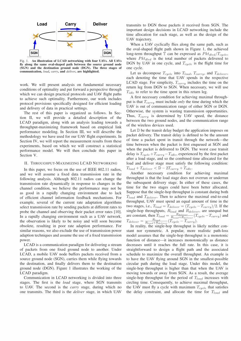
Fig. 1. An illustration of LCAD networking with four UAVs. All UAVsfly along the same oval-shaped path between the source ground node(SGN) and the destination ground node (DGN). The three stages ofcommunication, load, carry, and deliver, are highlighted.

work. We will present analysis on fundamental necessaryconditions of optimality and put forward a perspective throughwhich we can design practical protocols and UAV flight pathsto achieve such optimality. Furthermore, our work includesprotocol provisions specifically designed for efficient loadingand delivery of data in practical settings.

The rest of this paper is organized as follows. In Sec-tion II, we will provide a detailed description of theLCAD paradigm, along with an analysis leading towards athroughput-maximizing framework based on empirical linkperformance modeling. In Section III, we will describe themethodology we have used for our UAV flight experiments. InSection IV, we will report the measurement results from theseexperiments, based on which we will construct a statisticalperformance model. We will then conclude this paper inSection V.

II. THROUGHPUT-MAXIMIZING LCAD NETWORKING

In this paper, we focus on the use of IEEE 802.11 radios,and we will assume a fixed data transmission rate in thefollowing analysis. Although 802.11 radios can change thetransmission rate dynamically in response to changes in thechannel condition, we believe the performance may not beas good in a rapidly changing environment due to lackof efficient channel information feedback mechanisms. Forexample, several of the current rate adaptation algorithmsselect transmission rate by sending packets at different rates toprobe the channel and observing their packet error rates [10].In a rapidly changing environment such as a UAV network,the observation is likely to be noisy and will soon becomeobsolete, resulting in poor rate adaption performance. Forsimilar reasons, we also exclude the use of transmission poweradaption techniques and assume the use of a fixed transmissionpower.

LCAD is a communication paradigm for delivering a streamof packets from one fixed ground node to another. UnderLCAD, a mobile UAV node buffers packets received from asource ground node (SGN), carries them while flying towardsthe destination, and finally delivers them to the destinationground node (DGN). Figure 1 illustrates the working of theLCAD paradigm.

Communication in LCAD networking is divided into threestages. The first is the load stage, where SGN transmitsto UAV. The second is the carry stage, during which noone transmits. The third is the deliver stage, in which UAV

transmits to DGN those packets it received from SGN. Theimportant design decisions in LCAD networking include thetime allocation for each stage, as well as the design of theUAV trajectory.

When a UAV cyclically flies along the same path, such asthe oval-shaped flight path shown in Figure 1, the achievedlong-term throughput T can be expressed as Pktdlvd/Tcycle,where Pktdlvd is the total number of packets delivered toDGN by UAV in one cycle, and Tcycle is the flight time forone cycle.

Let us decompose Tcycle into Tload, Tcarry, and Tdeliver,each denoting the time that UAV spends in the respectiveLCAD stage. For simplicity, Tcarry includes the time on thereturn leg from DGN to SGN. When necessary, we will useTidle to refer to the time spent in this return leg.

A first necessary condition for achieving maximal through-put is that Tcarry must include only the time during which theUAV is out of communication range of either SGN or DGN.Otherwise, the system is wasting transmission opportunities.Thus, Tcarry is determined by UAV speed, the distancebetween the two ground nodes, and the communication rangeof the wireless devices used.

Let D be the transit delay budget the application imposes onpacket delivery. The transit delay is defined to be the amountof time a packet spent in transit through the network—thetime between when the packet is first enqueued at SGN andwhen the packet is delivered to DGN. The worst case transitdelay is Tcycle +Tcarry−Tidle, experienced by the first packetafter a load stage, and so the combined time allocated for theload and deliver stage must satisfy the following condition:Tload + Tdeliver < D − 2Tcarry + Tidle.

Another necessary condition for achieving maximalthroughput is that the load stage does not overrun or underrunthe subsequent delivery stage. In either of these cases, thetime for the two stages could have been better allocated.Suppose that the single-hop throughput is constant during bothTload and Tdeliver. Then to achieve the maximal end-to-endthroughput, UAV must spend an equal amount of time in thetwo stages, i.e., Tload = Tdeliver = (Tcycle −Tcarry)/2. If thesingle-hop throughputs, Rload and Rdeliver, are unequal butare constant, then Tload = Rdeliver

Rload+Rdeliver(Tcycle−Tcarry) and

Tdeliver = Rload

Rload+Rdeliver(Tcycle − Tcarry).

In reality, the single-hop throughput is likely neither con-stant nor symmetric. A popular, more realistic path-lossmodel assumes that the single-hop throughput is a monotonicfunction of distance—it increases monotonically as distancedecreases until it reaches the full rate. In this case, it isstraightforward to design a flight path and the associatedschedule to maximize the overall throughput. An example isto have the UAV flying around SGN in the smallest-possiblecircular path during the load stage. Under this model, thesingle-hop throughput is higher than that when the UAV ismoving towards or away from SGN. As a result, the averagesingle-hop throughput for the period of Tload increases withcircling time. Consequently, to achieve maximal throughput,the UAV must fly a cycle with maximum Tcycle that satisfiesthe delay constraint, and allocate the time for Tload and

Tdeliver according to the average single-hop throughput inthe respective stages. One can also trade delay for throughputbecause T increases as D increases.

We conclude that a good single-hop throughput model iskey for throughput-maximizing LCAD networking because itallows for optimal stage-time allocation and flight-path design.It also provides better insight into the delay-throughput trade-off. However, even a distance-based model described above istoo simplistic in the face of real-world factors such as relativeangles and polarization between the transmit and receiveantennas, perturbations in the UAV positions and attitudes,and Doppler effects associated with UAV speed. We will reportour evaluation of more detailed model including some of thesefactors in Section IV-A.

We may use multiple UAVs in a pipelined fashion, asillustrated in Figure 1. We can schedule these UAVs such that aUAV’s load stage always overlaps with the other UAVs’ carryor deliver stages, and that its deliver stage always overlapswith the other UAVs’ load or carry stages. However, when thenumber of UAVs exceeds a certain threshold, there could besome complications. For example, two adjacent UAVs couldbe so close to each other, in either the load or deliver stage,that there could be contention and interference between theirtransmissions. The use of LCAD with a large number of UAVsmerits further investigation.

III. NETWORK TESTBED AND FLIGHT EXPERIMENTS

In this section, we describe our testbed setup and someflight experiments with LCAD. The testbed was built for thepurposes of evaluating LCAD throughput performance andcharacterizing the wireless links.

Fig. 2. (a) A custom-made dipole antenna installed on a ground node;(b) a dipole antenna installed beneath a UAV wing (inside a cardboardbracket); and (c) a GPS receiver mounted on a UAV wing.

Our networking testbed consisted of a UAV node and twoground nodes—SGN and DGN. These nodes were made upof single-board x86 computers made by Thecus, and wereequipped with Wistron CM9 802.11a/b/g adapters (Atheroschipset) with 18dBm transmit power. We used a custom-made2-dBi dipole antenna on all the nodes. The dipole antenna onthe ground node was vertically placed and elevated to about25 inches above ground (cf. Figure 2 (a)). The dipole antennaon the airplane was vertically placed beneath the wing (cf.Figure 2 (b)). The UAV was built from a Senior Telemastermodel airplane kit [11], and the computer equipment wasinstalled inside its body compartment. The two ground nodeswere placed on the opposite ends of the runway, separated by550 yards.

The UAV had an on-board GlobalSat BU-353 GPS receiver(cf. Figure 2 (c)), which provided position information at the

Fig. 3. A sample UAV path in the flight experiments projected ontoa U.S. Geological Survey (USGS) satellite map showing the locations ofSGN and DGN. The small squares show the per-second positions of theUAV as reported by its GPS. The light-colored horizontal band in thecenter of the map is an airport runway approximately 25 yards wideand 700 yards long.

resolution of 1 Hz. We had performed a coarse calibration ofthe GPS, and we found that errors in its reported coordinateswere normally within 5 meters. The UAV’s GPS trace and thestationary ground nodes’ coordinates allowed us to analyzevarious performance parameters as functions of distance andelevation angle.

The UAV flew in an oval-shaped flight path at an averagealtitude of 80 yards. An example of such path is shown inFigure 3. The airplane was operated by a human operator onthe ground through radio control. Even though the operatortried to follow a predetermined path, there were inevitablynoticeable variations in the actual path traversed.

The results reported in Section IV are based on the tracescollected in three flight runs that took place on two days oneweek apart. The first run lasted for 712 seconds on the first day.The second (380 seconds) and the third (637 seconds) runstook place on the second day. During these runs, the airplanecompleted a total of 20 round trips between the two groundnode sites. Although we tried to keep the testbed configurationidentical for both days, the weather conditions in terms ofwind speed and direction, as well as the airplane operatorswere different.

A. A Lightweight LCAD Protocol

Since the speed of the aircraft and the distance betweenSGN and DGN were known, we only needed to measurethe achieved single-hop throughput for the load and deliverstages in order to compute the overall achieved throughput.Thus, in our experiments, we used an empty carry stage andkept the UAV either in load or deliver stage. To decide thecurrent stage of the UAV node, a daemon process on the UAVnode computed the distances from its current GPS coordinatesto those of SGN and DGN, respectively. If the UAV wascloser to SGN than DGN, it would put itself in the loadstage. Otherwise, it would be in the deliver stage. The UAVconstantly broadcast beacons at a fixed interval (200 ms) toindicate which one of the two stages it was currently in.

When the UAV is in deliver stage, it sends data packets atfull rate to DGN until it enters load stage. If the SGN receivesbeacons indicating that the UAV is in load stage, it transmitsdata at full rate to UAV. SGN stops data transmission eitherwhen it receives beacons indicating that UAV is no longerin load stage, or after not receiving beacons for 3 consecutive

intervals (600 ms). It is important that SGN stops transmissionoutside of load stage because its transmission could contendwith that of UAV or interfere with reception at DGN. We notethat the LCAD protocol here uses a relatively small numberof beacon packets so as to minimize the pollution introducedon packet-error measurement and link characterization.

B. Trace Collection

In our experiments, all nodes used channel 11 of 802.11g,with the link-layer transmission rate fixed at 6 Mbps. All datapackets (1,500 bytes, including IP/UDP headers) and beaconpackets (64 bytes, including IP/UDP headers) were generatedwith sequence numbers. In addition, all packets were sentto a network broadcast address, so there was no link-layerretransmission. As a result, we will report the raw packet errorrate at the physical layer without ARQ (Automatic Repeat-reQuest). To shorten the control loop between UAV and SGN,we reduced the madwifi driver’s transmission queue size to4 packets and the Linux socket buffer size to 3 packets. Thesesettings reduced queueing in the operating system and avoidedexcessive delays for both beacon and data packets.

We also collected the timestamp and sequence number ofeach data or beacon packet sent and received. The timestampof a sent packet is generated when the socket function callsendto() returns, while that of a received packet is gener-ated when recvfrom() returns. In addition, UAV’s positionswere logged along with timestamps for interpolating distancebetween transmitter and receiver when a particular packet isreceived.

IV. EXPERIMENTAL RESULTS AND DISCUSSION

In this section, we will begin with a summary of LCAD per-formance measured during 20 complete cycles performed overthree runs. A detailed list of the results and time breakdownfor each stage is available in Table II of the Appendix. Wewill then continue with link characterization and constructionof statistical packet error models.

We first summarize the throughput utilization for the threeruns. The throughput utilization for each cycle is the ratioof the total number of packets delivered to DGN dividedby cycle time. The total number of packets delivered iscomputed by taking the minimum between the number ofpackets received by UAV and that by DGN—at most thatmany packets sent by SGN eventually reached DGN. Theresult shows that the average throughput utilization for thefirst run is 0.2283 ± 0.0369, 0.2837 ± 0.1345 for the secondrun, and 0.3176 ± 0.0278 for the third run.

From our earlier experience with 802.11g, we learnedthat the maximum distance between two ground nodes withsimilar configurations cannot exceed 50 yards if they needto communicate at a reasonably low packet loss rate using802.11g. In this testbed, it would take additional ten groundnodes to form a relay chain connecting SGN and DGN. Li andet al. reported that the throughput utilization of a 7-node relaychain using 802.11b radios is about 0.25 [1]. The throughputresults from the three runs show that LCAD can perform betterthan the traditional multi-hop ground relay chain.

We observe that the utilization is lower than the averagepacket error rate (PER) suggests. The average PER for thefirst run is 0.4223 for load stage and 0.3001 for delivery stage,0.105 and 0.3389 for the second run, and 0.1147 and 0.2426for the third run. These error rates should allow an even higherthroughput than measured. However, there is an additional lossof efficiency due to buffer underruns or overruns. Figure 4shows the histogram for the buffer occupancy of the 20 cycles.Negative buffer occupancy indicates that a buffer underrunoccurred, and the UAV node could have sent that many morepackets if the buffer were not empty. Positive buffer occupancyis the number of packets left in the UAV’s queue at the end of acycle. These packets will be discarded. The average number ofpackets delivered in a cycle is about 7000 packets, so the bufferoccupancy values in the figure indicate a serious imbalancebetween LCAD stages, which leads to a significant loss inutilization.

The average length of the cycles was 63 ± 8.7 seconds.Within these cycles, the time devoted to load and deliverstages of LCAD was slightly biased toward the load stage.The average ratio of Tload/Tdeliver was 1.23 ± 0.16.

Buffer occupancy (in thousands of packets)

1

2

3

4

5

6k to 7

k

5k to 6

k

4k to 5

k

3k to 4

k

2k to 3

k

1k to 2

k

0 to 1

k

1k to 0

2k to

1k

3k to

2k

4k to

3k

5k to

4k

Num

ber

of observ

ations

0

Fig. 4. Buffer occupancy histogram constructed from the 20 flightcycles. Negative values represent an idle, underutilized cycle, while themagnitude indicating the extent of the underutilization.

Figure 5 shows the details of the third cycle in the secondrun (labelled as “2-3”). The performance results are reported at1-second intervals for the purpose of investigating correlationat a finer granularity than the numbers reported in Table II.Among the six rows, the fifth row compares efficiency lossand modeled path loss. Efficiency loss incorporates packeterrors and halted SGN transmission due to lost beacons. Themodeled path loss is the amount of signal attenuation in dB,normalized with respect to the maximal observed attenuationin the experiments. Such attenuation is predicted by a free-space propagation model plus an approximate antenna gainpattern, which we will describe in more detail in the followingsection.

The fifth row shows the correlation between the efficiencyloss and modeled path loss. We do notice that there are dis-crepancies in some samples. For example, while the modeledpath loss does not change as much, PER increases sharplyaround 370 second in load stage and 402 second in deliverstage. We believe the discrepancies mainly result from aneffect of antenna cross-polarization when the UAV banks whilemaking a turn. There are other minor effects, such as velocityand ground reflection, that may contribute to efficiency loss.We will construct a statistical model to better quantify the

Fig. 5. Details of cycle 2-3. The left column contains results from loadstage, whereas the right column contains results from deliver stage. TheX-axis of the first five rows represents time offset into the run, and Y-axisshows either the measured performance or the settings of the flight pathin the stage. The first row shows the number of packets sent and lost atone second intervals. The second row plots the packet error rate at onesecond intervals. The third row plots the distance between transmitterand receiver, along with the UAV’s altitude above ground over time. Thefourth row depicts the UAV’s elevation angle relative to the ground nodeover time. The fifth row compares efficiency loss and modeled path loss.Lastly, the sixth row plots the UAV’s trajectory during the stage viewedfrom the top. The diamond marker indicates the location of the groundnode. The circles give the UAV’s locations projected onto the groundat the resolution of 1 Hz. The circles are drawn in increasing sizes astime progresses. The color represents PER during that second—red forhighest and blue for lowest PER.

correlation in the next subsection.

A. Link Characterization

In this subsection, we present an empirical model forlink performance prediction. Link performance models areof essential importance to throughput-maximizing flight-pathdesign. In order to help flight-path design, these models canonly use information that is available at design time. Thismay include characteristics of system components such aswireless transceiver and antenna. It may also include trajectoryof UAV, which can be obtained at the output of the flight-path design and used in the next design iteration. It can notuse, for example, instantaneous signal strength because thatinformation is not available prior to flight. Because of this, ourmodel will predict link performance for the particular systemat hand solely based on UAV trajectory information.

From trajectory, we first derive two important factors that

influence link performance. The first one is the distancebetween the UAV and ground nodes. In many models, distanceis the only factor considered. The second factor is the elevationangle φ of the UAV, as seen by the ground node, which plays arole because we use vertical dipole antennas. Specifically, φ isdefined as the angle between the direction of the antenna andthe incident direction of the radio waves from the UAV. Forexample, φ = 0 when the UAV is directly above the groundnode. In this case, the link performance is usually very poorbecause the UAV and ground nodes are in the antenna “null”of each other [12]. We can confirm this by looking closelyinto the visualization of one of the cycles in Figure 5.

We will combine the effect of these two factors into avariable called the “modeled path loss.” First, because theUAV usually maintains a line of sight to the ground node thatit intends to communicate with, the free-space propagationmodel should give a good prediction on the propagation loss.On top of that, we will add the signal loss due to the elevationangle φ perceived by the ground node, computed as follows.The magnitude of the electrical field due to radiation froma half-wavelength dipole antenna at an elevation angle φ isapproximately proportional to cos(π

2 cos φ)/ sin φ [12], whichcan be further approximated to |E(φ)| = sinφ. Combiningthese two losses together, we will have the modeled path loss:L = 20 log10 f+20 log10 d−20 log10 (|E(φ)|)−147.56, wheref is the central frequency of the channel [12].

We will use efficiency loss instead of packet error rate as ourperformance metric because the latter tends to underestimatethe true packet error rate when SGN is not transmitting dueto lost beacons. We will seek a complete statistical charac-terization of the relationship between modeled path loss andefficiency loss using the multivariate kernel density estimationtechnique [13].

Recall that a multivariate kernel density estimator withkernel k and window width h is defined by

f̂(x) =1

nhd

n∑i=1

k

(1h

(x − xi))

,

where xi ∈ Rd,∀i = 1, 2, . . . , n, are the observations, nthe number of observations, d the dimension of x, and f̂an estimate of the joint probability density function of x =(x1, x2, . . . , xd). We will use the multivariate Gaussian kernel:

k(x) =1

d√

2πe−

12xT x.

The choice of the window width h for the multivariateGaussian kernels will follow the rules of thumb described bySilverman [13].

We briefly give our intuition behind the density estimationtechnique. We assume that the observed samples are drawnfrom an unobserved distribution. We could use a multi-dimensional histogram to approximate the density function.However, due to error and noise in observation and measure-ment, each sample may have actually been contributed bythe probability mass from its vicinity regions. The histogramwill need to be “smoothed” somehow to properly take intoaccount such erroneous offsets. Also, in the case of continuous

random variables such as path loss and efficiency loss, thereare numerous “gaps” between samples. We will need a wayto “interpolate” the histogram for the values that are missingfrom the observations. The kernel density estimate techniqueprovides a way to smooth and interpolate histograms. Thekernel function serves as the weighing function in averagingthe contributions from neighboring samples for predicting theprobability density for a particular point. The choice of widthis important because it determines the size of the neighbor-hoods for averaging and thus will influence smoothness andfidelity of the resulting density estimate. As pointed out bySilverman [13], there does not appear to be a universallygood way of choosing this width. All methods are makingcertain trade-offs in one kind or another. In our case, we haveexperimented with several different ways of width choosingbefore we eventually settled down to our decision. Our choiceappears to be able to produce reasonable results that agree withour experience with and understanding of the testbed system.

We are now ready to state our modeling approach. Foreach run, we randomly select about half of the cycles as thetraining set. We use the multivariate Gaussian kernel densityestimation technique to produce an estimate for the jointprobability density of modeled path loss and efficiency loss inthis training set. Based on this estimated density, we computethe conditional mean efficiency loss conditioning on modeledpath loss and use it as the predictor for efficiency loss givenmodeled path loss. Figure 6 shows a few example predictors

80 85 900

0.2

0.4

0.6

0.8

Modeled path loss (dB)

Effi

cien

cy lo

ss

80 85 900

0.2

0.4

0.6

0.8

Modeled path loss (dB)

Effi

cien

cy lo

ss

Fig. 6. The estimated mean efficiency loss, derived from different trainingsets chosen randomly from the measurement data, as a function ofmodeled path loss for the load (left) and deliver (right) stages in thethird run in Table II. The different colored curves in each plot representdifferent training sets. The similarity in these curves shows that ourapproach is rather robust to the choice of training sets.

produced by this approach. We show the mean efficiency lossobtained using different training sets from the third run inTable II. We note that first, predictors obtained using differenttraining sets are very similar, so our approach is robust in thesense that it is rather insensitive to the choice of training sets.Secondly, we tend to have a higher efficiency loss when thelink quality is poor in the load stage. This is because loss of 3consecutive beacons can result in efficiency loss of 1 for thenext beacon period. It could also be because the source anddestination ground nodes are not symmetric in terms of theirrelative positions with respect to the UAV flight trajectory,as well as the difference in hardware components of thesetwo nodes due to inevitable variations in manufacturing anddeployment.

Figure 7 shows several samples of estimated probabilitydensities of efficiency loss for various modeled path losses.

Training set Our model Distance FixedCycle 1–5 6.42% 14.88% 56.75%Cycle 6–10 2.50% 4.56% 36.21%Cycle 1,2,5,6,8 5.50% 1.32% 14.82%

TABLE I

The percentage errors between predicted and measured average bufferoccupancies for the three models using different training sets from thethird run in Table II. Our model not only produces predictions withsmaller error, but also has a robust performance that is insensitive to thechoice of training sets. Distance-based model can also perform quitewell sometimes, showing that distance is indeed the most importantperformance determining factor.

These plots shows that the general quality the prediction basedon modeled path loss is reasonably good. If the conditionaldensity under a particular modeled path loss is highly con-centrated around a certain value, then the prediction error inthis case will be small. Contrarily, if the density spreads outacross a wide range of modeled path losses, like the curvescorresponding to the higher path losses in the load stage inFigure 7, the prediction can not be very accurate.

We further quantitatively evaluate the effectiveness of ourapproach by measuring how good it is in predicting bufferoccupancies. For each training set, we use the efficiencyloss predicted by our model to compute the average bufferoccupancy for the remaining cycles. We then compare theprediction with the measured buffer occupancy. We also makesimilar predictions using two other straightforward models thatemploy a number of commonly used techniques for predictingthe packet loss rate. The first one is solely based on distance.Specifically, we divide distance into ten fixed-sized bins anduse the average efficiency loss in each bin obtained from thetraining set to predict the efficiency loss in the rest of thecycles. We call this model the “Distance” model. The secondmodel is even simpler—we just predict that the efficiency lossin the rest of the cycles will be the same as the averageefficiency loss in the training set. We call this model the“Fixed” model. Table I shows the error percentage betweenpredicted and measured average buffer occupancies for thethree models using different training sets from the third run inTable II. We can see that our model significantly outperformsthe simple Fixed model in that the errors are much smaller.The performance of the Distance model, on the other hand,

0 0.2 0.4 0.6 0.8 10

0.5

1

1.5

2

2.5

3

Efficiency loss

Estim

ate

d p

robabili

ty d

ensity

L=80 dBL=83 dBL=86 dBL=89 dB

0 0.2 0.4 0.6 0.8 10

0.5

1

1.5

2

2.5

3

Efficiency loss

Estiam

ted p

robabili

ty d

ensity

L=80 dBL=83 dBL=86 dBL=89 dB

Fig. 7. The estimated conditional probability densities of efficiency lossunder several different modeled path losses for the load (left) and deliver(right) stages. The general quality of the prediction is fairly good, as canbe seen from the high concentration of probability mass around thepeaks in most curves. However, the precision of the prediction does dropas modeled path loss increases.

is fairly close to that of our model. Furthermore, althoughour model usually performs better, we do see a situation asshown in the last training set where distance does a better job.This conforms with the wide-accepted intuition that distanceis the most important factor in determining the performanceof a wireless link. However, its performance is less robustacross different training sets. The error can be quite significantsometimes, as shown by the first training in Table I. We believethat this is because of its failure of taking elevation angles intoaccounts in this case.

V. CONCLUSION

In this paper, we presented the load-carry-and-deliver(LCAD) networking paradigm that is specially designed formaximizing the throughput of UAV-relaying networks. Onenecessary condition for throughput maximization in suchnetworks is having no overruns or underruns in the UAVnode’s buffer. To achieve throughput maximization in practice,we will need a performance model for the communicationchannel, so that we can adjust flight paths in order to minimizethe surplus or deficit. This is especially so for our case becausethe COTS radios we used are not designed and engineered forthe rapid changing UAV networking environment.

By using model airplanes and IEEE 802.11g radios, weperformed several sets of experiments for the purpose ofevaluating LCAD performance, as well as collecting data forderiving an empirical link performance model. The measuredperformance suggests that the proposed LCAD paradigm canbe used to provide high throughput communication betweentwo ground nodes, as compared with the conventional multi-hop, store-and-forward relay chain. The reason for such aresult is that we can schedule UAV’s transmissions to avoidinterference and medium access contention. The trade-off isthe higher packet delivery latency. We also showed that themodel we derived from several randomly selected trainingsubsets can predict the buffer occupancy of the rest of the dataset with small errors. This is an encouraging result becauseit suggests COTS radio can potentially be used in LCADapplication scenarios.

In summary, the contributions we made in this paper in-clude: (1) the design of a light-weight LCAD protocol; (2) theanalysis on a few fundamental necessary optimality conditions;(3) UAV flight experiments and throughput measurementsfor LCAD; (4) demonstrating LCAD’s throughput advantageover conventional wireless multi-hop relay protocols; (5) anempirical performance model for predicting the achievableLCAD throughput for UAV networks; and (6) the feasibility ofusing low-cost COTS radio for UAV networking applications.

REFERENCES

[1] J. Li, C. Blake, D. S. J. D. Couto, H. I. Lee, and R. Morris, “Capacityof ad hoc wireless networks,” in ACM MobiCom, July 2001.

[2] C. M. Cheng, P. H. Hsiao, H. T. Kung, and D. Vlah, “Parallel Use ofMultiple Channels in Multi-hop 802.11 Wireless Networks,” in IEEEMILCOM, October 2006.

[3] A. Cerpa, J. L. Wong, L. Kuang, M. Potkonjak, and D. Estrin, “Statisticalmodel of lossy links in wireless sensor networks,” in ACM/IEEE FourthInternational Conference on Information Processing in Sensor Networks(IPSN05), April 2005.

[4] W. Zhao and M. H. Ammar, “Message Ferrying: Proactive Routingin Highly-Partitioned Wireless Ad Hoc Networks,” in FTDCS ’03:Proceedings of the The Ninth IEEE Workshop on Future Trends ofDistributed Computing Systems (FTDCS’03), 2003, p. 308.

[5] W. Zhao, M. Ammar, and E. Zegura, “A Message Ferrying Approach forData Delivery in Sparse Mobile Ad Hoc Networks,” in ACM MobiHoc,May 2004, pp. 187–198.

[6] ——, “Controlling the Mobility of Multiple Data Transport Ferries in aDelay-Tolerant Network,” March 2005.

[7] D. Henkel and T. X. Brown, “On Controlled Node Mobility in Delay-Tolerant Networks of Unmanned Aerial Vehicles,” in InternationalSymposium on Advance Radio Technolgoies (ISART), March 7-9, 2006.

[8] E. W. Frew, T. X. Brown, C. Dixon, and D. Henkel, “Establishmentand Maintenance of a Delay Tolerant Network through DecentralizedMobility Control,” in IEEE International Conference On Networking,Sensing and Control, April 23-25, 2006, pp. 584–589.

[9] P. Gupta and P. R. Kumar, “The Capacity of Wireless Networks,” IEEETransactions on Information Theory, vol. 46, no. 2, pp. 388–404, March2000.

[10] M. Lacage, M. H. Manshaei, and T. Turletti, “IEEE 802.11 RateAdaptation: A Practical Approach,” in MSWiM ’04: Proceedings of the7th ACM international symposium on Modeling, analysis and simulationof wireless and mobile systems, 2004, pp. 126–134.

[11] “Senior Telemaster R/C Airplane by Hobby Lobby International, Inc.”http://www.hobby-lobby.com/srtele.htm, 2006.

[12] R. C. Johnson, Antenna Engineering Handbook. McGraw-Hill Profes-sional, 1992.

[13] B. W. Silverman, Density Estimation for Statistics and Data Analysis.Chapman & Hall/CRC, 1986.

APPENDIX

In Table II, we report the performance and time duration foreach individual stage, as well as the UAV’s buffer occupancyfor each cycle, the cycle time Tcycle, and the overall through-put. The packet error rate (the PER column) is computedfrom number of packets sent and received in each stage.The length of the stage in seconds is reported in the Tload

and Tdeliver columns. The dist column reports the averagedistance in meters between transmitter and receiver during thestage and is computed from the GPS log and ground nodes’locations. lost and sent columns report the total numberof lost and sent packets in that stage. The last four columnsrecord the total number of packets delivered by the UAVunder LCAD (dlvd), the UAV’s buffer occupancy at the endof the cycle (BO), the cycle time Tcycle, and the utilization.The total number of packets delivered is computed by takingthe minimum between the number of packets received bythe UAV and that by DGN. Buffer occupancy records thenumber of packets left in the buffer at the end of the cycle.A number inside parentheses means that the UAV could havesent that many more packets if the buffer were not depleted.In other words, buffer underrun has occurred, and the numberquantifies the degree of underrun. To get a better sense ofthroughput performance, we report the utilization in additionto the packet delivery rate of the cycle. From the analysis ofcollected traces, the average send rate from the transmitteris at most 398 packets per second. For these reasons, thereported utilization is calculated as packet delivery rate dividedby 400 packets per second. An average row is inserted intothe table after each run to report aggregated average distancesand the average utilization of all cycles in that particular run.

load stage deliver stage overallcycle PER Tload dist. lost sent PER Tdeliver dist. lost sent dlvd BO Tcycle utilization (pkt/s)1-1 0.4756 40.815 200 5340 11227 0.3445 32.192 168 4367 12675 5887 (2421) 73.007 0.2016 (80.636)1-2 0.4143 40.819 198 4421 10672 0.3906 36.040 165 5518 14126 6251 (2357) 76.859 0.2033 (81.330)1-3 0.4486 39.012 194 4351 9700 0.3081 35.014 165 4280 13890 5349 (4261) 74.026 0.1806 (72.259)1-4 0.3891 41.016 191 4869 12514 0.1828 28.970 155 2103 11503 7645 (1755) 69.986 0.2731 (109.236)1-5 0.4264 40.028 176 4840 11352 0.3808 29.980 169 4522 11875 6512 (841) 70.008 0.2325 (93.018)1-6 0.3797 43.059 196 4987 13135 0.1939 29.995 163 2297 11845 8148 (1400) 73.054 0.2788 (111.534)average 198 164 0.2283 ± 0.03692-1 0.1133 42.015 144 1870 16498 0.2486 28.963 140 2840 11422 8582 6046 70.977 0.3023 (120.912)2-2 0.0658 38.026 130 970 14752 0.2771 24.981 122 2670 9635 6965 6817 63.008 0.2764 (110.542)2-3 0.1186 33.009 122 1503 12675 0.4790 36.019 126 6766 14126 7360 3812 69.029 0.2666 (106.623)2-4 0.1223 25.855 138 1245 10182 0.3509 22.130 149 3005 8563 5558 3379 47.985 0.2896 (115.829)average 144 134 0.2837 ± 0.13453-1 0.2050 29.006 128 2126 10370 0.2572 22.038 149 2070 8048 5978 2266 51.044 0.2928 (117.115)3-2 0.1273 30.008 117 1389 10908 0.1959 28.014 136 2022 10320 8298 1221 58.022 0.3575 (143.015)3-3 0.0572 32.077 129 694 12135 0.2353 29.014 138 2502 10632 8130 3311 61.091 0.3327 (133.081)3-4 0.0813 36.820 146 1140 14022 0.1885 27.041 142 1873 9938 8065 4817 63.861 0.3157 (126.289)3-5 0.0606 32.070 133 735 12128 0.2985 24.065 135 2589 8673 6084 5309 56.135 0.2710 (108.382)3-6 0.1180 31.833 128 1368 11597 0.2027 26.010 138 1940 9570 7630 2599 57.843 0.3298 (131.910)3-7 0.0995 29.076 126 1057 10627 0.1856 28.010 132 1902 10250 8348 1222 57.086 0.3656 (146.236)3-8 0.1544 30.009 131 1695 10980 0.3432 30.011 120 3767 10975 7208 2077 60.020 0.3002 (120.093)3-9 0.1444 25.855 123 1379 9548 0.2564 22.020 149 2061 8039 5978 2191 47.876 0.3122 (124.865)3-10 0.0995 31.009 126 1146 11512 0.2622 25.024 145 2381 9081 6700 3666 56.032 0.2989 (119.574)average 129 138 0.3176 ± 0.0278

TABLE IIPerformance summary of the 20 cycles from 3 test runs. The “cycle” column indicates the run and the sequence of the particular cycle in that run.The “PER” column shows the overall packet error rates. The “dist.” column is the average distance between the UAV and ground nodes. The “lost”and “sent” columns show the total number of packets lost and sent during that cycle, whereas the “dlvd” column is the total number of packetsdelivered from SGN to DGN via UAV during that cycle. The “BO” column shows the UAV’s buffer occupancy at the end of that cycle (number inparenthesis is deficit), and the “utilization” column is the normalized throughput based on the number of packets delivered and the length of thecycle. The three “average” rows summarize the average distance and the average utilization for that particular run.