maximum likeihood method for estimating airplane stability ... · advantages and disadvantages of...
TRANSCRIPT

NASA I
LOAN COPY: RETURN TO TP AWL TECHNICAL LIBRARY 1637 KlRTLAND AFB, N.M. c,l
NASA Technical Paper 1637
I
C.
Maximum Likelihood Method for Estimating Airplane Stability and Control Parameters From Flight Data in Frequency Domain
Vladislav Klein
MAY 1980
L.
https://ntrs.nasa.gov/search.jsp?R=19800015831 2020-01-10T16:32:58+00:00Z
TECH LIBRARY KAFB, NM
I lllllllllll lllll lllll lllll lllll lllllllll Ill1 . .. 0134027
NASA Technical Paper 1637
Maximum Likelihood Method for Estimating Airplane Stability and Control Parameters From Flight Data in Frequency Domain
Vladislav Klein The George W~isbirigtoii Uriizlersity
Joirit I i i s t h t e for Advaiiceiiieiit of Flight Scierices La rigley Resed rch Ceri ter Haii ip to 11, Virgiri ia
NASA National Aeronautics and Space Administration
Scientific and Technical information Office
1980

Y
SUMMARY
A f requency domain maximum l i k e l i h o o d method is developed f o r t h e estima- t i o n o f a i r p l a n e s t a b i l i t y and control parameters from measured da ta . model of an airplane is represented by a d i sc re t e - type s t eady- s t a t e Kalman f i l t e r with t i m e variables rep laced by t h e i r Four i e r series expansions. The l i k e l i - hood func t ion of innovat ions is formulated, and by its maximization wi th respect to unknown parameters t h e e s t i m a t i o n a lgor i thm is obta ined . This algo- rithm is then s i m p l i f i e d to t h e output error es t imat ion method wi th t h e d a t a i n t h e form o f t ransformed t i m e h i s t o r i e s , frequency response curves , or spectral and cross-spectral d e n s i t i e s . The development is followed by a d i s c u s s i o n on t h e equiva lence o f t h e cost f u n c t i o n i n t h e t i m e and frequency domains, and on advantages and d isadvantages of t h e frequency domain approach. The algorithm developed is app l i ed i n four examples to t h e e s t i m a t i o n of l o n g i t u d i n a l param- eters of a gene ra l a v i a t i o n a i r p l a n e us ing computer-generated and measured d a t a i n t u r b u l e n t and st i l l a i r . The cost func t ions i n t h e t i m e and frequency domains are shown to be equ iva len t ; t h e r e f o r e , both approaches are complemen- t a r y and n o t con t r ad ic to ry . Despite some computat ional advantages of parameter e s t ima t ion i n t h e frequency domain, t h i s approach is l i m i t e d to l i n e a r equa- t i o n s of motion wi th c o n s t a n t c o e f f i c i e n t s .
The
INTRODUCTION
The e a r l y approaches to t h e e x t r a c t i o n o f a i r p l a n e s t a b i l i t y and c o n t r o l parameters from f l i g h t d a t a were based on simple semigraphical or a n a l y t i c a l methods. Some of t h e s e methods used measured frequency response curves which provided good i n s i g h t i n t o t h e phys ics of t h e system and reduced d a t a process- ing to t h e use of s imple a lgeb ra . One of t h e f i r s t attempts to ana lyze mea- sured da ta i n t h e frequency domain f o r ob ta in ing t h e c h a r a c t e r i s t i c s of t h e shor t -per iod l o n g i t u d i n a l motion of an a i r p l a n e w a s made i n r e f e r e n c e 1 . I n r e fe rence 2 t h e same cha rac t e r istics were es t imated e i t h e r by f i t t i n g t h e mea- sured frequency response curves or by s u b s t i t u t i n g t h e measured d a t a i n t h e t r a n s f e r func t ion equat ion and minimizing t h e r e s u l t i n g error. I n both cases t h e l ea s t - squa res technique was appl ied . The same technique w a s used f o r t h e d i r e c t e s t ima t ion of t h e l o n g i t u d i n a l and l a t e r a l aerodynamic parameters i n r e fe rences 3 and 4 , r e s p e c t i v e l y .
The r eg res s ion wi th complex v a r i a b l e s was developed i n r e fe rence 5 and appl ied to t h e e s t i m a t i o n of a i r p l a n e t r a n s f e r func t ion c o e f f i c i e n t s from mea- sured frequency response curves. A more gene ra l formula t ion of t h e r eg res s ion i n t h e frequency d m a i n w a s in t roduced i n r e f e r e n c e 6 and extended to t h e maxi- mum l i k e l i h o o d method i n r e fe rence 7. I n both cases t h e procedure w a s used f o r t h e des ign of an optimal inpu t f o r system i d e n t i f i c a t i o n r a t h e r than f o r param- eter e s t ima t ion .
With t h e a v a i l a b i l i t y o f modern d i g i t a l computers, t h e f requency domain f o r a i r p l a n e parameter e s t i m a t i o n w a s almost f o r g o t t e n and t h e measured d a t a

have been mostly analyzed in the time domain. However, some further research and applications in this area have appeared. New frequency domain methods for system identification based on the equation-error formulation were introduced in reference 8 . Frequency domain data were used for the extraction of param- eters of an elastic airplane in reference 9, of parameters of an airplane with nonsteady aerodynamics in references 10 and 11, and of flying qualities crite- ria in reference 12.
The material contained in this report is an extension of the research ini- tiated in reference 5 and continued in references 6 and 7. Also included in this report are some of the developments and results from references 13 and 14, respectively. The purpose of this report is to present a rigorous development of an algorithm for the maximum likelihood estimation of airplane parameters in the frequency domain. The report also briefly points out the relationships between the estimation in the time and frequency domains, and the advantages and disadvantages of the frequency domain approach, mainly in terms of appli- cability, computing complexity, and accuracy of final results. The development starts with the formulation of a steady-state Kalman filter for a linear dynam- ical system. Before the log-likelihood function of the innovations is formu- lated, the basic properties of a complex random number and random sequence are presented. The log-likelihood function is minimized by using the modified Newton-Raphson technique. The maximum likelihood algorithm is then simplified by neglecting external disturbances to the airplane. Following the discussion, four examples are presented. They deal with the simplified longitudinal motion of a general aviation airplane and use both computer-generated and real-flight
SYMBOLS
sensitivity matrix
reading of vertical accelerometer, g units
covariance matrix of residuals
pitching-moment coefficient, My/&SC
vertical-force coefficient, F~/:S
wing mean aerodynamic chord, m
constants in differential equation for Gauss-Markoff process
matrix of transformed-system equations
expected value
matrix of continuous system
force along vertical body axis, N

G
GW
9
H
K11,12,.
k1,2,. .
R
Rzz I
control matrix of continuous system
process-noise distribution matrix of continuous system
acceleration due to gravity, m/sec2
transformation matrix
identity matrix
moment of inertia about lateral body axis, kg-m2
log-likelihood function
= \I-1
Kalman-filter-gain matrix
. . , 3 3 elements of K matrix
.,lo constants in equations of motion
Fisher information matrix
pitching moment, N-m
transformed quantity at mth and nth interval, respectively
mass, kg (in appendix D)
number of data points
covariance matrix of state variables
probability
probability density
process-noise covariance
rate of pitch, rad/sec
1
2 kinetic pressure, -PI2,
ma tr ix
N/m2
measurement-noise covariance matrix
correlation function of z
number of output variables
3

S
T
U
v
V
W
wg
X
Y
z
zn
a
E
0
v
P
02
wing area, m2
cross-spectral density of y and u
spectral density of z
quantity a t s t h , t t h , and T t h interval, respectively
transfer-function matrix
control vector
true airspeed, m/sec
measurement- no i se vector
process-noise vector
vertical component of turbulence velocity, Wsec
s ta te vector
measurement vector
random variable rea l or complex
= e x p ( j q $
angle of attack, rad
angle of attack measured by w i n d vane, rad
control matrix of discrete system
process-noise distribution matrix of discrete system
elevator deflection, rad
Kronecker delta
arbitrary small number
vector of unknown parameters
pitch angle, rad
innovat ion vector
a i r density, kg/m3
variance (a is standard deviation)
4
i
d

@ t r a n s i t i o n ma t r ix
phase ang le of complex v a r i a b l e y , deg
phase-angle c h a r a c t e r i s t i c s r e l a t i n g y and u v a r i a b l e s , deg
'PY
'PYU
w angular f requency, rad/sec
w0 = a/N
Aerodynamic d e r i v a t i v e s ( r e fe renced to a system o f body axes w i t h t h e o r i g i n a t the a i r p l a n e c e n t e r of g r a v i t y ) ;
a - d -
ac' = -
''&e a&,
def ined i n appendix D (eqs. (D5) to (D8) ) &,c&, 1 S u b s c r i p t s :
C cont inuous system
E measured q u a n t i t y
9 g u s t
k k t h e lement of vec to r or k t h column of ma t r ix
R Rth element o f vec to r or % t h row of matrix
m vector c o n s i s t i n g of a l l e lements up to and inc luding m
0 i n i t i a l va lue
5

Super scr ip t s :
T transpose matrix
-1 inverse matrix
estimated value
transformed variable
n
M
derivative w i t h respect to time
* transpose complex conjugate matrix
R real part
I imaginary part
Ma thema t ica l m ta ti on :
Tr trace of matrix
Re real part of complex number
I I de terminan t
- amplitude-ratio characteristic relating and u variables
U
A increment
ESTIMATION ALGORITHM
For the development of the estimation algorithm it is necessary f i r s t to postulate the model of an airplane and then to transform t h i s model into the frequency dmain. of innovations and its maximization w i t h respect to the unknown parameters. T h i s step leads to the iterative scheme for parameter estimation, which updates the previous estimates by employing the second- and first-order gradients of the log-likelihood function.
The next step is the formulation of the likelihood function
The linear airplane equations of motion are assumed i n discrete-time form to be
x( t+ l ) = o x(t) + r u(t) + rw w(t) (t = 0,1, . . ., N - 1 ) (1 1
y ( t ) = H x ( t ) + v ( t ) (t = O,l, . . ., N - 1 ) (2)
6
P

where x ( t ) is a state vec to r , u ( t ) is a c o n t r o l vec to r , w ( t ) is a process-noise v e c t o r , y ( t ) is an o u t p u t v e c t o r , and v ( t ) is a measurement- no i se vec tor .
I t is assumed t h a t
(a) Q, r, rw, and H are c o n s t a n t matrices
(b) Q is stable
(c) (@,r) and (Q,rw) are c o n t r o l l a b l e p a i r s
(d) (@,H) is observable
(e) w and v a r e s t a t i o n a r y , Gaussian uncor re l a t ed no i se sequences wi th
E{v( t ) w T ( T ) ) = 0 f o r a l l t and T
( f ) N is even
In t h e g e n e r a l case t h e unknown parameters w i l l occur i n t h e matrices Q, r, rw, H, Q, R, x(O), and Po. Their e s t i m a t i o n may be extremely d i f f i - c u l t because of the a lgo r i thm complexity (see r e f . 15) and possible i d e n t i f i - a b i l i t y problems (see r e f . 1 6 ) . The system parameter e s t i m a t i o n w i l l be s i m p l i f i e d by formula t ing a s t e a d y - s t a t e Kalman-f i l ter r e p r e s e n t a t i o n of equa t ions (1 ) and (2) and by cons ide r ing t h e unknown parameters i n t h i s r ep resen ta t ion .
The c o n d i t i o n a l expected va lue of t h e state vec to r is de f ined as
7

The innovat ions are de f ined as
V ( t ) = y ( t ) - H z ( t )
and t h e covar iance ma t r ix of state v a r i a b l e s is de f ined as
Then t h e s t eady- s t a t e Kalman-f i l ter r e p r e s e n t a t i o n o f t h e system described by equa t ions (1) and (2 ) is
Reference 17 shows t h a t t h e innovat ions V ( t ) form a sequence of independent Gaussian v e c t o r s wi th
The d e f i n i t i o n of t h e ga in ma t r ix K i n equat ion ( 9 ) can be found i n r e f e r - ence 15 or 16 i n t h e form
B = HPHT +
p = @POT -
For t h e f u r t h e r
R (1 3)
T KBKT + rd rw (1 4)
development of t h e i d e n t i f i c a t i o n a lgo r i thm a l l t i m e func- t i o n s i n equat ions ( 9 ) and (10) are w r i t t e n i n terms of their Four i e r series expansions. As stated i n appendix A, t h e Four i e r series expansion o f random v a r i a b l e s holds i n t h e mean-square sense . I f t h e Four i e r series component of x ( t ) is def ined as
8

f o r
N
2 1 . . ., O r 1 , - I - -
2lT
N Lere 00 = - , and similar y f o r t h e o t h e r v a r i a b l e s , equat,Jns ( 9 ) and (10)
transformed from t h e t i m e to t h e frequency domain have t h e form
zn Z(n) = H(n) + I’ G(n) + K O(n)
I n equat ion (16) zn = exp(jnwo), which fo l lows from t h e r e l a t i o n s h i p
assuming t h a t x ( 0 ) = x(N) = 0. As proved i n appendix A, t h e transformed inno- v a t i o n s 3 (n) are uncor re l a t ed , orthogonal, and Gaussian random v a r i a b l e s with
E{g(n)) = 0 I where SYL, is t h e spectral d e n s i t y o f V ( t ) , and g*(n) is t h e complex conju- gate of gT(n ) . It fo l lows from equa t ions (16) and (17) t h a t
G(n) = H ( Z n 1 - a)-’ r G(n) + [H (ZnI - K + I1 g i n )
= T1 (n,@ z ( n ) + T2(n,@) G(n)
9

i f 1
(20) I
where I is the i d e n t i t y ma t r ix , T1 and T2 are t h e system t r a n s f e r func- t i o n s def ined as
I
T~ (n,O) = H(Z,I - 6)-1r
T2(nr@) = H(Z,I - Q ) - ~ K + I I
and @ is t h e vec tor o f unknown parameters i n equa t ions (9) and (10) . Equa- i t i o n (19) is i n v e r t i b l e i n t h e sense t h a t p ( n ) can be solved f o r d i r e c t l y I
i n terms of g ( n ) and 0 (n) i n terms of p ( n ) (see ref. 1 8 ) . This implies t h a t T2 is nonsingular . Therefore , from equat ion (19)
To o b t a i n t h e l i ke l ihood func t ion , i.e., t h e j o i n t p r o b a b i l i t y d e n s i t y of t h e transformed innovat ions 0 [n) (assuming t h a t a l l parameters are known), a vec to r 0, c o n s i s t i n g o f all innovat ions up to and inc lud ing frequency m is introduced. Therefore
Assuming t h a t t h e p r o b a b i l i t y d i s t r i b u t i o n of 0, has a d e n s i t y p[gm], then it follows from t h e d e f i n i t i o n of c o n d i t i o n a l p r o b a b i l i t i e s t h a t
Repeated u s e of t h i s formula g i v e s t h e express ion f o r t h e l i k e l i h o o d func t ion as
Because t h e d i s t r i b u t i o n of 0(m) is Gaussian, then t h e d i s t r i b u t i o n of 0 ( m ) g iven g(m-1) is also Gaussian; i.e.,
10

as follows from the definition of a complex multivariate distribution in appen- dix B. In equation (26) r is the dimension of the innovation vector.
Using equation ( 2 6 ) the logarithm of equation (25 ) can be written as
In the log-likelihood function given by equation ( 2 7 ) , the unknown parameters are the elements of the matrices @ , r , H, K, and S w . An estimate of the unknown parameters is obtained by minimizing the log-likelihood function from the feasible set of parameter values. Optimizing the log-likelihood function for parameters in Syv gives
N --1 2
where Cn = >. The estimates of the remaining unknown parameters are given N 2
n=- -
by the root of the equation
A
for %V replaced by SW. This root can be found by a modified Newton-Raphson iteration (e.g., ref. 19) as
11

h
where t h e step s i z e @ f o r parameter estimates is given by
The index 0 a t t h e ma t r ix M i n d i c a t e s t h a t i t s elements were computed for 0 = 00. I n equa t ion (31) M is t h e F i s h e r information m a t r i x
M = -E{ a25 (0) ] a@ a@
Because t h e step s i z e f o r parameter estimates is a v e c t o r w i th real elements on ly , and t h e log - l ike l ihood f u n c t i o n is real , t h e expres s ions f o r t h e f i r s t - and second-order g r a d i e n t s of J(0) are also real; i.e.,
aJ (0) aij (n) - - - -2N Re In V* (n) S;: -
a 0 k %k
and
(33)
The expres s ions for t h e elements o f t h e information m a t r i x and t h e gradi- e n t of t h e log-l ikel ihood f u n c t i o n are developed i n appendix C i n t h e form
and
a J (0) -
(36)
12

where
are t h e estimates of i npu t spectral d e n s i t i e s and cross-spectral d e n s i t i e s , r e spec t ive ly .
The f i n a l estimates of unknown parameters have t h e fo l lowing properties (see r e f s . 20 and 21):
They are c o n s i s t e n t ; i.e.,
(wi th E a r b i t r a r i l y s m a l l )
They are a sympto t i ca l ly unbiased; i. e.,
and they are a sympto t i ca l ly e f f i c i e n t wi th
A
E{ (6 - 0) (0 - h -E
Because o f equa t ions (32) and ( 3 8 ) , t h e inve r se of t h e information mat r ix pro- v ides t h e Cramgr-Rao lower bounds on t h e va r i ance and covar iance of errors i n t h e es t imated parameters.
OUTPUT ERROR METHOD
I f t h e process noise is z e r o and t h e i n i t i a l states are assumed to be equa l i d e n t i c a l l y to ze ro , i.e., w ( t ) = 0 , x ( 0 ) = 0, and P ( 0 ) = 0 , t h e s ta te -covar iance m a t r i x is also zero. Then, as follows from equa t ions (12) and (211, t h e Kalman g a i n s are z e r o and T2 = I. The innovat ions are reduced to output errors
13

1 f where T(n,@o) is equa l to T1 (n,@) def ined by equa t ion ( 2 0 ) . For 00 -+ 0
t h e innovat ions O(n) + ?(n) and SvV -+ S,. The expres s ions f o r t h e elements of t h e information ma t r ix and g r a d i e n t of t h e log- l ike l ihood func t ion are obta ined by s impl i fy ing equa t ions (35) and (36) as
I N
L n=- - 2
and
The express ions f o r t h e information ma t r ix and t h e g r a d i e n t of t h e log- l i k e l i h o o d func t ion can also be e a s i l y der ived from t h e s i m p l i f i e d log- l i k e l i h o o d func t ion , which takes t h e form o f t h e o u t p u t error cost f u n c t i o n
These express ions are
M(@) = 2N Re En A*(n) S z A(n)
a J (0) -1 - - - -2N R e E, A* (n) S, 3 (n) ao
where A(n) is t h e s e n s i t i v i t y ma t r ix whose elements are equa l to a rT(n,@o) G(n) I/%%.
I n some experiments a i r p l a n e t r a n s f e r f u n c t i o n s are measured d i r e c t l y us ing a harmonic inpu t or are determined from measured input-output t i m e h i s t o r i e s . Then t h e cost func t ion inc ludes a t r a n s f e r f u n c t i o n error r a t h e r t han an ou tpu t error. The cost func t ion is t h e r e f o r e formed as
(43)
(44 )

where T is a vec tor which inc ludes system t r a n s f e r f u n c t i o n s as elements. These t r a n s f e r func t ions are computed from equat ion (20) f o r a g iven 00.
Both cost f u n c t i o n s ( 4 2 ) and (45 ) can be minimized wi th respect to unknown parameters i n a, G, and H or w i t h respect to t r a n s f e r func t ion c o e f f i c i e n t s i n T. The estimates are ob ta ined from equa t ions ( 3 1 ) , (43) , and ( 4 4 ) ; t h e spectral d e n s i t i e s are g iven by equa t ion (28) us ing p e r t i n e n t r e s idua l s .
For a system wi th a s i n g l e inpu t , t h e o u t p u t error cost f u n c t i o n wi th mea- su red t r a n s f e r f u n c t i o n s (frequency response curves) is de f ined as
I n t h i s formula t ion t h e scalar v a r i a b l e ing func t ion express ing t h e r e l i a b i l i t y of t he measured data according to t h e harmonic con ten t of an input .
G(n) may be i n t e r p r e t e d as a weight-
DISCUSSION
The frequency domain i d e n t i f i c a t i o n has s e v e r a l features which are d i s t i n c t They are mainly associated wi th t h e model repre- from t h e t i m e domain approach.
s e n t a t i o n and e s t i m a t i o n algorithm. There is, however, t h e equiva lence i n t h e cost func t ion used i n t h e t i m e and frequency domains as expressed by Pa rceva l ' s theorem. This theorem p o s t u l a t e s t h e r e l a t i o n s h i p between t h e squared magni- tudes of the Four i e r t ransform pairs. I t t h e r e f o r e states t h a t t h e t i m e domain cost func t ion ,
N- 1
t = O where 2, = >, is equa l to t h e frequency danain cost func t ion ,
Using equat ion (15 ) the frequency domain cost func t ion can be w r i t t e n as
15

N- 1
T=O where cT = >. But according to appendix A,
= o
(for t = T)
(for t # T)
The equivalence of both approaches is no longer valid if the frequency domain cost function is restricted to a given frequency range. Such a restriction is not necessary, but it is an option which is a strong point in favor of fre- quency domain analysis with respect to time domain analysis. The selected frequency range of interest was used, for example, in reference 9, where air- plane rigid modes were separated from elastic ones. For similar results in the time domain the data must be filtered accordingly.
The early airplane estimation techniques in the frequency domain were using measured frequency response curves only. This approach could have an advantage when repeated measurements under the same conditions are available. A hypothesis concerning the model adequacy can be tested using the variance estimates from scatter around the mean and from residuals (ref. 5). On the other hand the simultaneous analysis of repeated maneuvers for obtaining a single set of estimates with increased accuracy can also be applied to directly measured or transformed time histories. In general, transformed input-output time histories are preferred in frequency domain parameter estimation. The inaccuracies of frequency response curves computed from transformed inputs and outputs can be quite pronounced for frequencies in which the harmonic content of an input is close to zero.
The transformation of model equations into the frequency domain replaces differentiation and convolution with multiplication. As a result the sensitiv- ity equations in the nonlinear estimation algorithm are reduced to uncoupled algebraic expressions. This simplification can be appreciated mainly in cases for which convolution integrals are included in the equations of motion (ref. 11).
The computational differences between the time and frequency domains dis- cussed so far could be viewed as advantages of the frequency domain analysis. There is, however, a substantial disadvantage of the airplane identification in the frequency domain. This approach is limited, for practical reasons, to only linear equations of motion with constant coefficients. The computing time needed for parameter estimation in the frequency domain (transformation of mea- sured data included) is about 50 percent more than in the time domain. The assessment was obtained from the number of equations used in both domains for one iteration when the algorithms were applied to the system of equations with- out convolutions and process noise.
16
The e s t ima t ion a lgo r i thm w a s developed f o r a l i n e a r d i scre te - t ime model. The a i r p l a n e equa t ions of motion are, however, u s u a l l y given i n a cont inuous form as
x = Fx + Gu + Gww (49)
where t h e unknown parameters can be i n t h e matrices F, G, and %. For t h e cont inuous model (eq. ( 4 9 ) ) , t h e expres s ions f o r t h e information mat r ix and g r a d i e n t of t h e log- l ike l ihood func t ion remain t h e same as equat ions (35) and (36). B u t now t h e t r a n s f e r func t ions are def ined as
~ ~ ( w , e ) = H ( j w 1 - ~ 1 - 1 ~ (50
T2(w,8) = H ( j w 1 - F)"KC + I (51
where t h e Kalman-fil ter-gain mat r ix is obta ined from t h e r e l a t i o n s h i p s (see, e .g . , r e f . 22)
K, = PHTR-~ z
and
FP + PFT - PHTR-~HP + % ~ ~ ~ l t ; = o
I n t h e model formula t ion it was assumed t h a t t h e i n i t i a l cond i t ions were e q u a l to zero, t h a t t h e model descr ibed a s t a b l e motion of an a i r p l a n e , t h a t there were no a p r i o r i known va lues of s t a b i l i t y and c o n t r o l parameters , and t h a t the measurement noise w a s Gaussian and uncorre la ted . I f t h e i n i t i a l con- d i t i o n s d i f f e r from ze ro , t h e a d d i t i o n a l term H(z,I - @)- ' x(0 ) would have to be included i n equat ion (19) or t h e new t r a n s f e r func t ion H ( j w 1 - F)-l x ( 0 ) would have to be added to those def ined by equa t ions (50 ) and (51 ) . Then t h e vector of unknown parameters can be augmented by t h e vec tor of i n i t i a l condi t ions .
I f t h e a i r p l a n e motion inc ludes an uns t ab le mode, t h e parameter e s t i m a t i o n s t i l l can proceed provided t h a t t h e degree of i n s t a b i l i t y is not high. A l a r g e i n s t a b i l i t y , on t h e o t h e r hand, can r e s u l t i n excess ive t r a n s i e n t motion due to nonzero i n i t i a l cond i t ions and/or t h e inpu t and thus l i m i t t h e v a l i d i t y of t h e l i n e a r equat ions of motion. I f t h e a pr ior i mean va lues and va r i ances of some parameters are known, they can be included i n t h e e s t ima t ion procedure. I n t h i s case t h e cost f u n c t i o n must be expanded i n a s imilar way a s i n d i c a t e d i n r e fe rence 19.
The maximum l i k e l i h o o d method developed ear l ier assumed a Gaussian, uncor- r e l a t e d measurement noise . I f t h e random sequence r ep resen t ing t h i s no i se is c o r r e l a t e d , t h e e s t i m a t i o n a lgor i thm does n o t change. The c o n s t a n t va lues of
17

spectral d e n s i t i e s Svy or Svv are merely rep laced by t h e frequency depen- den t va lues es t imated from expres s ions similar to equat ion (37).
EXAMPLES 9 As examples t h e parameters o f a small g e n e r a l a v i a t i o n a i r p l a n e were esti-
mated from computer-generated d a t a and from measured d a t a i n s t i l l and turbu- l e n t a i r . (Some of t h e d a t a f o r examples 1 , 3 , and 4 are from r e f . 14.) For , a l l examples t h e model o f t h e a i r p l a n e was based on s i m p l i f i e d l o n g i t u d i n a l equa t ions of motion wi th t h e atmospheric tu rbulence ( g u s t s ) approximated as a Gauss-Markoff process of f i r s t o rde r . The model equa t ions (cont inuous form) are developed i n appendix D. When t h e state and o u t p u t equa t ions (D4) and (D9) are transformed i n t o t h e frequency domain and rear ranged , they have t h e form
t
The s t a t e and o u t p u t v e c t o r s are specified as 0-
j ; = [a Ggl
where t h e r a n d m inpu t is assumed to be a Gaussian, uncor re l a t ed n o i s e process wi th E{w} = 0 and E{w2) = CJg. The matrices i n equa t ions (52) and (53) are formulated as
L o 0 j w + c1
Gw = 0 -k c Co 1 ms
18

H =
k9 +lo
0 1
The known constants k1, k2, . . . ? klor cl, and c2, and the pitching- moment derivatives $, cI;ls, Cgq, and are defined in appendix D. (% e
Example 1
The output data were computed from equations (D4) and (D9) for given inputs 6, and w (with Og = 1 m/sec) and for a given set of parameters. To the computed time histories of output variables, an uncorrelated and Gaussian measurement noise was added. The measurement-noise standard errors were selected as
Ool = 0.0028 rad Oq = 0.0063 rad/sec UaZ = 0.029
The time histories of the input and output variables are plotted in figure 1. For the estimation algorithm these data were transformed into the frequency domain using the Filon integration formula. The sampling interval of the transformed data was 1.047 rad/sec. The transformed data were truncated at the frequency interval k20.944 rad/sec because outside this interval their amplitudes were very small.
The steady-state Kalman filter representation of the airplane motion described by equations (52) and (53) is
It was assumed that the parameters c1 and c2: the initial conditions, and the variances of the process and measurement noise were known. Also assumed as known was the parameter
Czs because of the identifiability problem.
19
The las t assumption is s u b s t a n t i a t e d by t h e small effect of t h e term on t h e airplane motion. The vector of unknown parameters w a s t h e r e f o r e formed as
k8c1Gq
i
' i where K11, K12, . . ., and K33 are t h e elements of t h e Kalman-fil ter-gain 1
m a t r i x Kc. The i n i t i a l va lues of t h e s e elements were computed from equa- t i o n s (50) and (51) .
F i r s t , t h e unknown parameters were determined by t h e maximum l i k e l i h o o d method developed. I n tab le I t h e estimated s t a b i l i t y and c o n t r o l parameters are compared wi th t h e i r t r u e va lues , and t h e estimated Kalman g a i n s are com- pared with t h e i r i n i t i a l va lues . eters is, i n g e n e r a l , very good. The e s t ima ted va lues of t h e Kalman g a i n s d i f f e r s i g n i f i c a n t l y from t h e i r i n i t i a l v a l u e s , and t h e s t anda rd errors (lower bounds) of t h e s e parameters are q u i t e high. T h i s i n d i c a t e s l o w accuracy o f t hese estimates. When, however, t h e Kalman g a i n s were f i x e d on t h e i r i n i t i a l value, t h e e s t i m a t e s of t h e a i r p l a n e parameters were f a r t h e r from t h e t r u e va lue , as i n d i c a t e d by results i n t h e f o u r t h column of table I. The las t set of a i r p l a n e parameters was ob ta ined by cons ide r ing no process no i se e f f e c t on t h e o u t p u t data. These estimates are also less accurate than t h o s e ob ta ined by t h e maximum l i k e l i h o o d method wi th a l l 15 unknown parameters. Table I also inc ludes t h e va r i ance estimates of t h e r e s i d u a l s . ahe l imi t ed expe r i ence ob ta ined from t h i s example i n d i c a t e s t h a t for s t a b i l i t y and c o n t r o l parameter e s t i m a t i o n f r a n data wi th pronounced e f f e c t of t h e process n o i s e (i.e., Ug b 1 m / s e c ) , t h e a lgo r i thm i n its complete form should be used and t h e Kalman f i l t e r g a i n s should be treated as t h e a d d i t i o n a l unknown parameters.
The agreement between t h e f i r s t set of param-
Example 2
I n t h i s example t h e measured data i n t u r b u l e n t air were used i n t h e same model as i n t h e previous example. The measured input-output time h i s t o r i e s are p resen ted i n f i g u r e 2. For t h e parameter e s t i m a t i o n t h e transformed data were taken from t h e frequency i n t e r v a l k9.817 rad/sec. The s t anda rd error of t h e v e r t i c a l g u s t v e l o c i t y was determined from t h e part of t h e measured data wi th 6, = Constant to be IJ = 1.12 m / s e c . The v a l u e s f o r measurement-noise s tan- dard errors were taken ?ran t h e r e s u l t s i n r e f e r e n c e 23 as
= 0.0017 rad Uq = 0.005 rad/sec U = 0.Olg u a V a,
The estimated s t a b i l i t y and c o n t r o l parameters are given i n t h e t h i r d and f o u r t h columns of table 11. I n t h e f i r s t case ( f o u r t h column) t h e Kalman g a i n s were treated as unknown parameters; i n t h e second case ( t h i r d column) they uere set equal to z e r o (assumption of no process noise). The i n c l u s i o n o f t h e pro- cess no i se i n t h e model r e s u l t e d i n b e t t e r accuracy of t h e parameter
20
Ck, as

i nd ica t ed by its comparison wi th t h e average va lue obta ined from the estimates i n t h e t i m e domain (see r e f . 23). On t h e o t h e r hand, t h e process-noise consid- e r a t i o n i n t h e e s t i m a t i o n process degraded t h e estimates of t h e parameters and cI;ls. N o exp lana t ion f o r t h i s degrada t ion could be found.
I
Example 3
From t h e measured t i m e h i s t o r i e s i n s t i l l a i r which are presented i n f i g - u re 3, t h e t ransformed i n p u t and o u t p u t d a t a and t h e frequency response cu rves r e l a t i n g a l l t h r e e o u t p u t s to t h e e l e v a t o r d e f l e c t i o n were obtained. By s e t t i n g
and t h e matrices D, H, and G were s i m p l i f i e d accordingly. The unknown parameters were es t ima ted from t h e minimizat ion of t h e cost func t ion , given by equat ion (42) for t h e transformed d a t a and by equa t ion (45) f o r t h e frequency response curves.
c w = 0 t h e state vec tor i n equa t ions (52) and (53) was changed to x = [a,qIT
The estimated parameters are g iven i n t h e s i x t h and seventh columns of table 11, and they are compared wi th t h e r e s u l t s from t h e t i m e domain estima- t i o n given i n t h e f i f t h column of t h e same t ab le . The t h r e e sets o f estimates from t h e same f l i g h t agree w e l l . The s t anda rd errors of t h e estimates i n t h e frequency domain are, however, h igher t han those i n t h e t i m e domain. Th i s could be due to t r u n c a t i o n o f t h e transformed data and a d d i t i o n a l i naccurac i e s i n measured frequency response curves caused by t ak ing t h e ratios of t w o com- p lex numbers. The t ransformed data and those computed are p l o t t e d i n f i g u r e 4; t h e measured and computed frequency response curves are plotted i n f i g u r e 5. Both f i g u r e s i n d i c a t e some modeling errors i n t h e equat ion f o r I t .is also apparent from f i g u r e 5 t h a t t h e measured frequency response curves are inaccu- rate around t h e frequency 6.4 rad/sec as a r e s u l t of t h e l o w harmonic con ten t of t h e inpu t a t t h e same frequency.
aV.
Example 4
The response of t h e a i r p l a n e to turbulence w a s measured i n t w o f l i g h t s (des igna ted run 1 and run 2 i n t a b l e 11) with t h e minimum p i lo t i n t e r f e r e n c e (6, = 0 ) . t r a l d e n s i t y o f t h e v e r t i c a l g u s t v e l o c i t y
s i t i es S
t r a n s f e r func t ion r e s u l t i n g from equa t ions (52) and (53).
From t h e t i m e h i s t o r i e s of t h e measured ou tpu t v a r i a b l e s t h e spec- and t h e cross-spectral den- s,$%
and Sw a were computed. They are related by t h e a i r p l a n e . wgq g z
( The state and output equa t ions were modified i n t h e fo l lowing way:
(a) I n equa t ion (52) w and 6, were se t equa l to ze ro
(b) wg w a s assumed as a known i n p u t
(c) The term k 8 c l w g w a s rep laced by -jWkgcQg
(d) I n equa t ion (53) % w a s set equa l to z e r o
21

The matrices D, G, and H were t h e r e f o r e changed as
H =
- 0 1
and t h e model was formulated as
Sw ,D = GSw 9 g g
SWgY = Hswgx + G
where
swgx - - [Swga SwgqIT
The vector of unknown parameters i n t h e s e equa t ions is formed as
(56)
(57)
The es t imated va lues of t h e f i r s t four parameters are given in t h e l a s t t w o columns of t a b l e 11. From t h e estimates of
22
% % and Co t h e va lue o f ms
w a s computed from equa t ions (D6) and (D7) and included among t h e unknown param- eters. The agreement between t h e resul ts from both runs is very good. The parameters also agree wi th t h e estimates from t h e still a i r measurement wi th t h e except ion of t h e parameter expected, probably because of some modeling errors i n equa t ions (56) and (57) .
CZa. Th i s parameter has a smaller va lue than
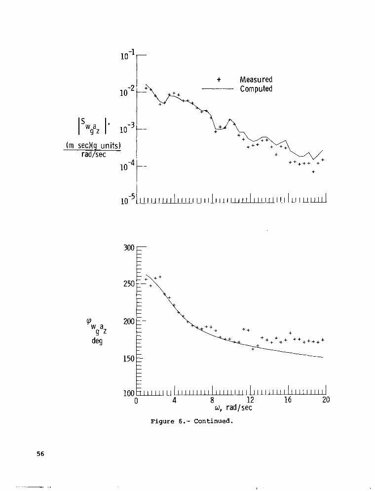
The measured spectral and cross-spectral d e n s i t i e s from run 1 and those computed by using t h e e s t ima ted parameters are p l o t t e d i n f i g u r e 6. I t w a s v e r i f i e d t h a t t h e large f i t error i n t h e phase of t h e cross-spectrum Sw d i d n o t a f f e c t t h e va lues of t h e e s t ima ted parameters s i g n i f i c a n t l y . Th:! esti- mate from turbulence and measurement demonstrates a p o s s i b i l i t y f o r us ing t h e s e d a t a also f o r a i r p l a n e s t a b i l i t y and c o n t r o l parameter e s t ima t ion . For c e r t a i n model formula t ions t h e d e r i v a t i v e o f pitching-moment c o e f f i c i e n t w i th respect to t h e rate of change i n a n g l e of a t tack can be e s t ima ted e x p l i c i t l y .
CONCLUDING REMARKS
A frequency danain maximum l i k e l i h o o d method h a s been developed f o r t h e e s t i m a t i o n o f a i r p l a n e parameters from measured f l i g h t data. A d i sc re t e - type s t eady- s t a t e Kalman f i l t e r w a s used i n t h e d e r i v a t i o n of t h e computing algo- ri thm. The t i m e v a r i a b l e s i n t h e model equa t ions were transformed i n t o t h e frequency danain by us ing a Four i e r series expansion. I f t h e i n i t i a l d a t a were Gaussian and uncor re l a t ed , t h e transformed data formed a complex random sequence which w a s uncor re l a t ed , o r thogonal , and Gaussian. Then, t h e l i k e l i - hood func t ion could be formulated as a m u l t i v a r i a t e d i s t r i b u t i o n of complex innovat ions.
The connect ion between t h e cont inuous form o f a i r p l a n e equat ions o f motion and t h e developed a lgo r i thm is e a s i l y e s t a b l i s h e d . The a lgor i thm can be s i m - p l i f i e d to t h e ou tpu t error method wi th t h e measured d a t a i n t h e form of t r ans - formed t i m e h i s t o r i e s , frequency response curves, or spectral and cross-spectral d e n s i t i e s . I n g e n e r a l , transformed input-output t i m e h i s t o r i e s are p r e f e r r e d i n frequency danain e s t ima t ion . The inaccurac i e s of frequency response curves computed from transformed i n p u t s and ou tpu t s can be q u i t e pronounced for f r e - quencies i n which t h e harmonic con ten t of an inpu t is close to zero. The f r e - quency domain approach s i m p l i f i e s t h e e s t ima t ion procedure by reducing t h e sen- s i t i v i t y equa t ions to simple a l g e b r a i c express ions . I t also provides an easier way than t h e t i m e domain f o r us ing t h e d a t a wi th in a frequency range of i n t e r - est. The serious disadvantage of t h e frequency domain i d e n t i f i c a t i o n is i n its practical l i m i t a t i o n to a system descr ibed by l i n e a r equat ions of motion wi th c o n s t a n t c o e f f i c i e n t s . I t w a s shown t h a t t h e cost f u n c t i o n s i n t i m e domain and frequency domain approaches are equ iva len t . I t is t h e r e f o r e necessary to con- sider both approaches as complementary and n o t con t r ad ic to ry .
The maximum l i k e l i h o o d method has been a p p l i e d to computer-generated and real f l i g h t d a t a f o r t h e l o n g i t u d i n a l motion of a small g e n e r a l a v i a t i o n air- p lane . I n t h e f i r s t case t h e estimates ob ta ined were more a c c u r a t e than those from the s i m p l i f i e d o u t p u t error method, which d i d n o t cons ider t h e e f f e c t of t h e process noise. I n t h e second case t h e r e s u l t s were inconclus ive because of an i n s u f f i c i e n t amount of measured da ta . Then, t h e s i m p l i f i e d algorithm was used w i t h t h e f l i g h t d a t a from measurements i n s t i l l a i r and t u r b u l e n t a i r wi th
23
$
t no pilot input. The first set of results for deterministic input showed the expected similarity in parameter values obtained from the time and frequency domains. The estimates from turbulence measurements demonstrated a possibility
estimation of the pitching-moment derivative with respect to the rate of change in angle of attack.
for using these data also for airplane parameter estimation and for explicit 4 I
i
Langley Research Center National Aeronautics and Space Administration Hampton, VA 23665 April 1, 1980
24
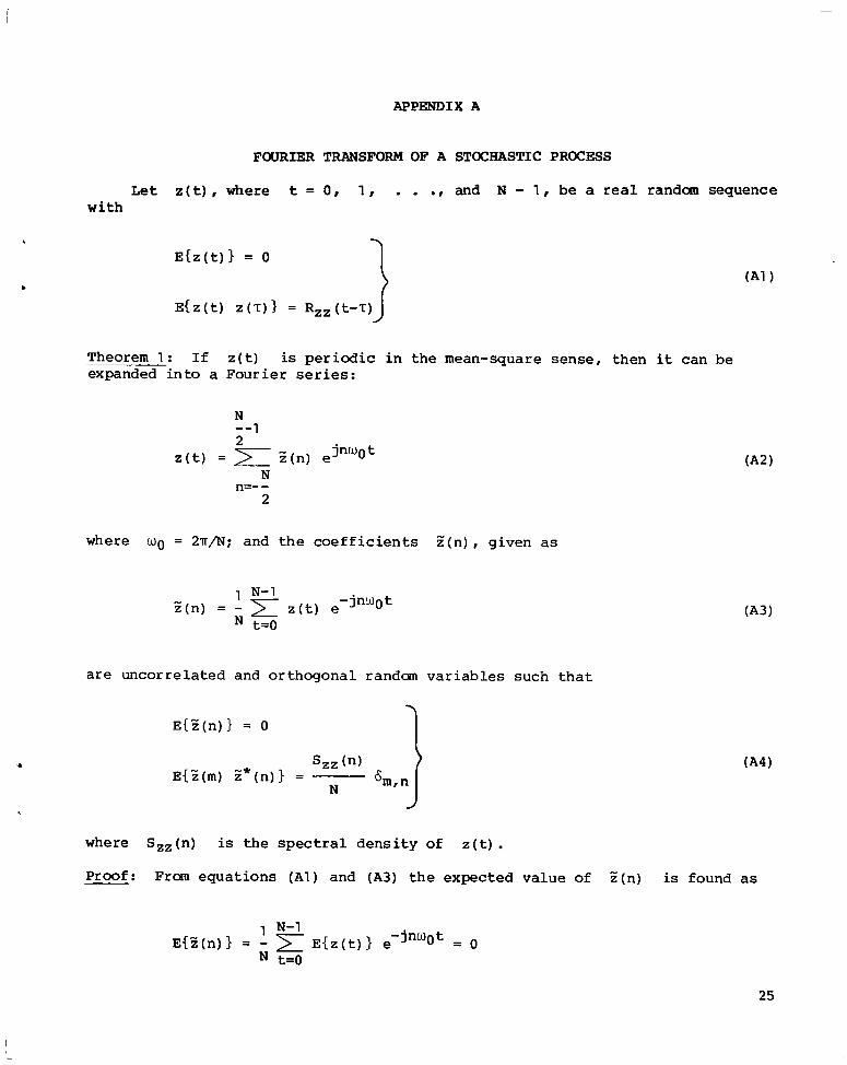
APPENDIX A
FOURIER TRANSFORM OF A STOCHASTIC PROCESS
L e t z ( t ) , where t = 0 , 1 , . . ., and N - 1 , be a real random sequence wi th
Theorem 1: I f z ( t ) is p e r i o d i c i n t h e mean-square sense , then it can be expanded i n t o a Four i e r series:
N --1
where wo = 2"; and t h e c o e f f i c i e n t s % ( n ) , given as
t = O
are uncorre la ted and or thogonal r a n d m v a r i a b l e s such t h a t
where S,,(n) is t h e spectral d e n s i t y of z ( t ) . Proof: Fram equa t ions ( A l ) and (A3) t h e expected va lue of Z(n) is found as
25

APPENDIX A
To prove t h e second part of equa t ion (A4) t h e conjugate of Z(n) is f i r s t m u l t i p l i e d by z ( t ) and then t h e expected va lue is taken; i.e.,
jnwo s E{z*(n) z ( t ) )
N
jnwos 1 N-1 = - E{z(t) z(s)) e
N s=o
The new v a r i a b l e T = t - s and t h e r e l a t i o n s h i p s
N - -1
are introduced (see, e.g., r e f . 6 ) . Then
Using equa t ions (A3) and (A7) t h e expected va lue of $ (m) z*(n) can be formulated as
4 i 1
+
26

APPENDIX A
For
For
m = n t h e r e is
m # n t h e d i f f e r e n c e m - n = a, where a is an in t ege r : t h e r e f o r e ,
and t h e proof of equat ion (A4) is t h u s completed.
T o prove equat ion ( A 2 ) , it is s u f f i c i e n t to show t h a t t h e sequence z ( t ) - t ends to En z ( n ) exp(jnw0t) i n t h e mean-square sense: i.e.,
N --1
n=- - 2
jnwo t
J e ) = O
The square i n equat ion (A9) can be w r i t t e n as a product of i t s e l f by i ts conjugate . Equation (A9) is t h e r e f o r e changed to
j (m-n) wo t = o + EnCm E{z(m) z"*(n)} e
I n t h e double summation a l l t h e terms with m # n are e q u a l to zero. Using equa t ions ( A l ) , (A2), and ( A 7 ) , t h e prev ious equat ion can be expressed as
Each sum above equa l s RZz(0) (see eq. ( A 5 ) ) ; hence t h e whole expres s ion equals ze ro and equat ion (A9) is proved.
27
I

1
i
j APPENDIX A !
Theorem 2: L e t z ( t ) , t = 0 , . . ., and N - 1 , be mutual ly s t o c h a s t i c a l l y independent random v a r i a b l e s having, r e s p e c t i v e l y , Gaussian d i s t r i b u t i o n s wi th E { z ( t ) ) = 0 and E { z 2 ( t ) ) = U2. Then t h e sequence
I' where
N N n = - -,. . . , O , l , . . .,- - 1
2 2
c o n s i s t i n g of real parts 'IzR(n) and imaginary parts ril(n) is a complex Gaussian and uncor re l a t ed sequence wi th
Proof: I t has a l r e a d y been proved t h a t
T h i s r e s u l t combined w i t h t h e d e f i n i t i o n of t h e expec ted .va lue of a complex r a n d m v a r i a b l e (eq. ( B l ) ) implies t h a t
I t has also been shown t h a t ( i n eq. ( A 8 ) )
$'
28
I I I

APPENDIX A
Using t h e same approach as t h a t f o r t h e development of equa t ion ( A 8 ) , it can be shown t h a t
+ jE{zR(m) Z1(n)) + jE{'il(m) ZR(n)} (A1 4 )
From equa t ions (A8) and ( A l 2 ) to ( A 1 4 ) , t w o sets of equa t ions can be formed as
J E{zR(m) Z R ( n ) ) - E{z"I(m) Z1(n)) = 0
and
These t w o sets g i v e t h e s o l u t i o n
s,, ( m ) E(zR(m) ZR(n) ) = E{zl(m) z l ( n ) ) = 6m,n
2N
which proves t h e v a l i d i t y of equa t ion ( A l l ) . Equations (A15) and (A16) have been developed f o r m and n being p o s i t i v e . I n t h e case where (-N/2) S m,n 6 (N/2 - 1 ) t h e proof based on t h e s e e q u a t i o n s is st i l l v a l i d .
29

APPENDIX A
The only change might occur in equations (AlS), where the right-hand sides would be interchanged. The form of the solution given by equations (A17) and (Al8) does not change.
Finally, it is necessary to prove that E(n) is Gaussian. For this proof the concept of the moment-generating function is used. is expressed as
When Z(n)
where
1 -jnwot c t = - e N
then the moment-generating function of the variable ct z(t) is given accord- ing to reference 24 as
where b is a constant independent of ct z(t). Thus, the moment-generating function of Z(n) is
- which means that z(n) is Gaussian with zero mean and variance 02/N or, using equation (A4), with variance S,,/N. The sequence z"(n) is formed by a collection of uncorrelated Gaussian random variables.
30

APPENDIX B
COMPLEX RANDOM VARIABLE
A complex random v a r i a b l e z is a complex number z ( 5 ) determined by an outcome 5 ; i .e.,
such t h a t t h e f u n c t i o n s zR and z1 a r e random v a r i a b l e s . By d e f i n i t i o n , t h e expected value of a complex random v a r i a b l e is
t h e va r i ance is
and t h e covar iance is
I f
then t h e complex random v a r i a b l e s 21 , 22, . . . , and zn a r e uncorrelated. They are or thogonal i f
I f t he complex randan v a r i a b l e z = zR + jzl has its real and imaginary parts normally d i s t r ibu ted wi th
31

APPENDIX B
and t h e s e parts are s t o c h a s t i c a l l y independent, then t h e d i s t r i b u t i o n of a complex random variable z w i l l be de f ined as a j o i n t d i s t r i b u t i o n of t h e independent v a r i a b l e s zR and z1 such t h a t
- - 1 exp ( -z*z/0:) - 2
TI02
I f z is a complex vec to r of dimension r , then t h e Gaussian d i s t r i b u t i o n is de f ined as
where 2 is t h e cova r i ance ma t r ix of z. This is a Hermitian nonnegative square ma t r ix of dimension r. If z has components t h a t are s t o c h a s t i c a l l y independent, then c is a d i agona l matrix. Equation (B5) a g r e e s with t h e d e f i n i t i o n of t h e Gaussian d i s t r i b u t i o n p resen ted i n r e fe rences 24 and 25.
32
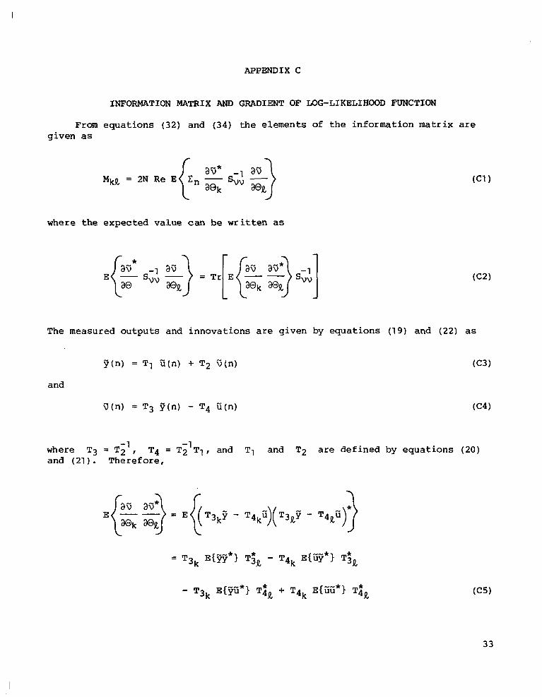
APPENDIX C
INFORMATION MATRIX AND GRADIENT OF LOG-LIKELIHOOD FUNCTION
From equa t ions (32) and (34) t h e elements of t h e informat ion ma t r ix are g iven as
MkR = 2N R e E { cn - aij* E} a o k %Q
where t h e expected va lue can be w r i t t e n as
The measured ou tpu t s and innovat ions are given by equa t ions (19) and (22) as
-1 -1 where T3 = T2 , T4 = T2 T I , and T1 and T2 are de f ined by equa t ions (20) and (21 ) . Therefore ,
33

where
... Because u (t) and V (t) are uncor re l a t eh , t h e transformed variables u (n) and u ( n ) are also uncorre la ted . Using equa t ions (C3) and (B4) t h e expected va lues i n (C5) can be expressed as
1
N E{Cfi*} = - Suu
After s u b s t i t u t i n g equat ion (C6) i n t o equat ion (C5) and some tedious manipulat ion,
From equat ions (C2) and (C7),
34
APPENDIX C
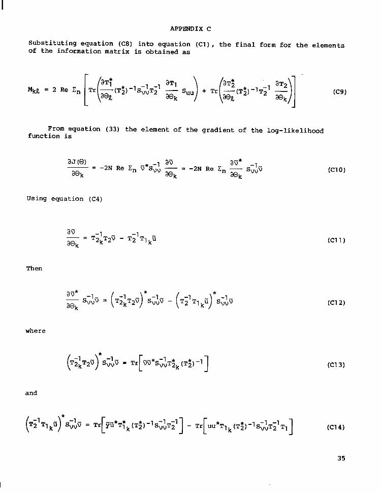
Substituting equation (C8) into equation (Cl) , the final form for the elements of the information matrix is obtained as
M a = 2 Re Cn -1
From equation (33 ) the element of the gradient of the log-likelihood function is
a J (0) -* -1 ao ao* -1- svvv
- - - -2N Re In v Svv - - - -2N Re In - a o k aok aok
Using equation (C4)
Then
where
aa - - - T-’T 3 - T;’T~ kfi a0k 2k
and
* (Ti’ T1 kO) S;:J = Tr yu T1 (TZ) -’ S;:Ti’] - Tr[ uu*T1 (T$) -’ SvvT2 -1 -1 TI] [--* *
35

1.1. 1 1 1 . 1 1 . --I, 111 ,,,..,., I...---- -.---
APPENDIX c
Int roducing
1 ,
N ...- * vv = - syy
1 A
N _- * uu = - s,,
-1 and approximating SvvsVv = I , equat ion (C12) is changed as
F i n a l l y , s u b s t i t u t i n g equat ion (C15) i n t o equat ion ( C l O ) , t h e e lements i n t h e g r a d i e n t vec tor are ob ta ined as
36

APPENDIX D
EQUATIONS OF LONGITUDINAL MOTION OF AN AIRPLANE IN PRESENCE OF TURBUL~NCE
The airplane equations of motion are referred to the body axes. They are perturbed equations for datum conditions corresponding to steady horizontal flight. The equations are based on the following assumptions:
(1 ) The airplane is a rigid body
(2) The elevator deflection and turbulence excite the longitudinal motion during which the airspeed remains constant
( 3 ) The turbulence is approximated by a one-dimensional gust field, and the angle-of-attack and pitch-rate perturbations due to turbulence are given as
and
qg = -“g
( 4 ) The aerodynamic model equations for the increments in Cz and Cm have the form
where the input and output variables are the increments with respect to the initial steady flight.
37

APPENDIX D
Using these assumptions, t h e l o n g i t u d i n a l equa t ions of motion can be expressed as
where g s i n 808 i n equat ion ( D l ) is n e g l i g i b l e .
I n equa t ions ( D l ) and (D2) ag is a s t o c h a s t i c va r i ab le . Its spectral d e n s i t y can be modeled, f o r example, by a Dryden formula (see r e f . 26) . I n t h e f u r t h e r development it w i l l be assumed t h a t t h e turbulence v e l o c i t y component
wg equat ion
is a Gauss-Markoff process of f i r s t o rde r governed by t h e d i f f e r e n t i a l
Gg = -C1Wg + c2w
where
6, is t h e scale of tu rbulence , and w is t h e uncor re l a t ed no i se process wi th Eqw} = 0 and E{w2} = 0;.
When equat ion ( D l ) is s u b s t i t u t e d i n t o equa t ion ( D 2 ) and equat ion (D3) is cons idered , then t h e s ta te equa t ions f o r t h e l o n g i t u d i n a l motion of t h e a i r - p lane w i l l have t h e form
38

I
APPENDIX D
w h e r e
P S k 3 = -
2m
pSV$ k 5 = -
2 I Y
p svoc k 7 = -
2 I Y
( N o t e : k4c2Czq = 0 ) .
p SC k 2 = -
4m
p SC k 4 = -
4mVo
p svoC2 k 6 =
41Y
p SC2 k 0 = -
41Y
39
APPENDIX D
c& = % - C6(l + $ cZq)
For the parameter estimation from measured data, state equations (D4) are completed by the output equations
40

REFERENCES
1. Milliken, William F., Jr.: Progress in Dynamic Stability and Control Research. J. Aeronaut. Sci., vol. 14, no. 9, Sept. 1947, pp. 493-519.
2. Greenberg, Harry: A Survey of Methods for Determining Stability Parameters of an Airplane From Dynamic Flight Measurements. NACA TN 2340, 1951.
3. Schumacher, Lloyd E.: A Method for Evaluating Aircraft Stability Param- eters Fran Flight Test Data. USAF Tech. Rep. No. WADC-TR-52-71, U.S. Air Force, June 9 952.
4. Donegan, James J.; Robinson, Samuel W., Jr.; and Gates, Ordway B., Jr.: Determination of Lateral-Stability Derivatives and Transfer-Function Coefficients Fran Frequency-Response Data for Lateral Motion. NACA Rep. 1225, 1955. (Supersedes NACA TN 3083.)
5. Klein, Vladislav; and Togovsk?, Josef: General Theory of Complex Random Variable and Its Application to the Curve Fitting a Frequency Response (Summary Report). 2PdVA VZLd 2-11, Dec. 1967.
6. Mehra, R. K.: Frequency-Domain Synthesis of Optimal Inputs for Linear System Parameter Estimation. Tech. Rep. No. 645 (Contract N00014-67-A-0298-0006) , Div. Eng. & Appl. Phys., Harvard Univ., July 1973.
7. Mehra, Raman K.: Synthesis of Optimal Inputs for Multiinput-Multioutput (MIMC)) Systems With Process Noise. System Identification - Advances and Case Studies, Raman K. Mehra and Dimitri G. Lainiotis, eds., Academic Press, Inc., 1976, pp. 211-249.
8. Gupta, N. K.: New Ftequency Domain Methods for System Identification. 1977 Joint Automatic Control Conference Proceedings - Volume 2, Inst. Electr. & Electron. Eng., Inc., 1977, pp. 804-808.
9. Rynaski, Edmund G.; Andrisani, Dominick, 11; and Weingarten, Norman C.: Identification of the Stability Parameters of an Aeroelastic Airplane. Technical Papers - AIAA Atmospheric Flight Mechanics Conference, Aug. 1978, pp. 20-27. (Available as AIAA Paper 78-1328.)
10. Kocka, Vila: Downwash at Unsteady Motion of a Small Aeroplane at Low Airspeeds - Flight Investigation and Analysis. ICAS Paper No. 70-25, Sept. 1970.
11. Queijo, M. J.; Wells, William R.; and Keskar, Dinesh A.: The Influence of Unsteady Aerodynamics on Extracted Aircraft Parameters. Technical Papers - AIAA Atmospheric Flight Mechanics Conference, Aug. 1978, pp. 132-139. (Available as AIAA Paper 78-1343.)
12. Twisdale, Thomas R.; and Ashurst, Tice A., Jr.: System Identification From Tracking (SIFT), a New Technique for Handling Qualities Test and Evaluation (Initial Report). AFFTC-TR-77-27, U . S . Air Force, Nov. 1977.
41

13. Klein, V.: Aircraft Parameter Est imat ion i n Frequency Domain. A Collec- t i o n of Technica l Papers - AIAA Atmospheric F l i g h t Mechanics Conference, Aug. 1978, pp. 140-147. (Avai lab le as AIAA Paper 78-1344.)
14. K le in , V.; and K e s k a r , D. A.: Frequency Domain I d e n t i f i c a t i o n of a Linear System Using M a x i m u m Likel ihood Estimation. Parameter Es t imat ion - F i f t h IFAC Symposium, Volume 2, R. Isermann, ed., Pergamon Pres s , Inc., c.1979, pp. 1039-1046.
I d e n t i f i c a t i o n and System
15. S tepner , David E.; and Mehra, Raman K.: Maximum Likel ihood I d e n t i f i c a t i o n and O p t i m a l Inpu t Design for Iden t i fy ing Aircraft S t a b i l i t y and Cont ro l Der iva t ives . NASA CR-2200, 1973.
16. Mehra, R. K.: I d e n t i f i c a t i o n i n Control and Econometrics; S i m i l a r i t i e s and Differences. Tech. Rep. No. 647 (Cont rac t NO001 4-67-A-0298-0006) , Div. Eng. & Appl. Phys., Harvard Univ., J u l y 1973. (Avai lable from DTIC as AD 767 393.)
17. Ka i l a th , Thanas: An Innovat ions Approach to Least-Squares Est imat ion - P a r t I: Linear F i l t e r i n g i n Addit ive White Noise. IEEE Trans. Autom. Control , vol. AC-13, no. 6 , D e c . 1968, pp. 646-655.
0
18. A s t r o m , Karl J.: In t roduc t ion to S t o c h a s t i c Cont ro l Theory. Academic Press , Inc. , 1970.
19. Taylor , Lawrence W., J r . ; and I l i f f , Kenneth W.: Systems I d e n t i f i c a t i o n Using a Modified Newton-Raphson Method - A FORTRAN Program. TN D-6734, 1972.
NASA
20. Kashyap, R. L.: Maximum Likelihood I d e n t i f i c a t i o n of S t o c h a s t i c Linear Systems. IEEE Trans. A u t o m a t . Contr. , vol. AC-15, no. 1 , Feb. 1970, pp. 25-34.
21. Eykhoff, P i e t e r : System I d e n t i f i c a t i o n - Parameter and S t a t e E s t i m a t i o n . John Wiley & Sons, c.1974.
22. Bryson, Arthur E., Jr.; and H o , Yu-Chi: Applied Optimal Control. Ginn and Co., c.1969.
23. Klein, Vladis lav: Determination of S t a b i l i t y and Control Parameters of a Light Airplane Fran F l i g h t Data Using Two Est imat ion Methods. TP-1306, 1979.
NASA
24. Miller, Kenneth S.: Complex S t o c h a s t i c Processes - An In t roduc t ion to Theory and Applicat ion. Addision-Wesley Pub. Co., Inc. , 1974.
25. Hannan, E. J.: M u l t i p l e Time Se r i e s . John Wiley & Sons, Inc. , c.1970.
26. E t k i n , Bernard: Dynamics of F l igh t . John Wiley & Sons, Inc. , c.1959.
42
I
TABLE I.- ESTIMATED AIRPLANE PARAMETERS FROM COMPUTER-GENERATED DATA
-. ... - .- . .-
I n i t i a l value
. . .. - . .
-5.0
- 20 -1 .o
-. 80 - 24 -3.3
-.0563
2.544
.0025
2.438
9.7
-.018
213.0
-5.065
-12.63
------I
- . - - . . .
Estimate of parameter (a)
With process noise - ~~
K estimated
-5.07 ._
(.091) -23.8 (2 03) -1.17
( .071) -. 82 (.015)
-24.0 (-52)
-3.21 (.062) -. 44 (.011) 2.31 (.010) -. 21 (.010) 1.84 ( .044)
10.8 ( ~ 4 ) .09 (-97)
156 (8-9) -8 (2.1 1
-15 (6 .2)
67
.30
50
K f i x e d -
-5.72 (.20)
-17 (2.7) -1 .l (-17) -. 94 (.031)
-25.5 ( 38)
-3.16 ( .080) -.0563
2.544
. 00 25 2.438
9.7
-.018
213.0
-5.065
-1 2.63
.72
.60
1 .l
Assumed no process noise
-5.2 (010)
-1 5 (4 -0 ) -. 57 (-31) -. 83 (.014)
-22.1 ( 65)
-3.18 (. 050) 0
0
0
0
0
0
0
0
0
.70
.82
1.6
aNumbers i n parentheses are Cramgr-Rao lower bounds on standard errors.
43

! . TABLE 11.- ESTIMATED AIRPLANE PARAMETERS FROM MEASUREMENTS I N TURBULENT AND STILL A I R
Parameter L Estimate of parameter
(a) Aver age value
and its standard
error (b)
Example 3 (st i l l a i r ) Example 2 (turbulent a i r )
Example 4 (turbulent a i r )
Frequency dmair (e 1
___i With
process noise
q domain
Assumed no pr oces s
noise
Frequency domain
(C)
F r equency domain
(dl Run 1 Run 2 ~
-5.3 f 0.1
-19 f 3
-1.2 2 0.2
-.80 f 0.02
f 0.4
-5.67 (. 057)
-10.3 ( 92) -.6 (-16) -.783 (. 0074)
(-40) -26.6
---------
-3.21 (. 030)
-5.70
-8 (3.5) -.6 .
( 0 28) -.81 (.011)
(-50)
(. 086)
-28.6
--------
-3.54 (. 040)
-5.6
-4 (4.7) -.6 ( * 33) -.82 (. 027)
(092)
(.I91
-26.3
-------- -3.38
(. 060)
-24.2
-8.0
-3.3 It: 0.05 -3.3 (-12)
aNumbers i n parentheses are Cram&-Rao lower bounds on standard errors. b ran the maximum likelihood estimates i n the time domain (ref. 23). 9ransformed input and output time histories. dFrequency response curves. eSpectral and cross-spectral densities.
and Co fCanputed fran estimated c% %I'

1. 0 E
Figure 1.- Time histories of computer-generated output and input variables.
45

111 I1 I I 1
.lo,
E- h
.25
q, rad/sec 0
-. 25
€ n
c
a,, g units 0
be, rad 0
c
b d 0 4 8 12 16
Time, t, sec
-. 05
Figure 2.- Time h i s t o r i e s of measured output and input var iables . F l i g h t i n turbulence.
46

.06-
a,, g uni t s
- Time, t, sec
Figure 3.- Time h i s t o r i e s of measured output and input var iables . F l i g h t i n still a i r .
47

rad
8i-10-2 + Measured output Computed output
4E J \;=
! ! ! ! ! ! I 1
w, rad/sec
Figure 4.- Measured transformed time histories and those computed by using estimated parameters .
48
I it rad/;ec
Measured Computed
output output
I-
5 E - L ‘t Obi 1 I I I I I I I1 I I I I I I1 I I I I I I I I I 1 I I I I I I I l l I I I I I l l I I I I I I
350 E f
5 0 b l I I I I I 1 I I I I I I I I I I I I I I I I I I I I I I I I I I I I I I I131 I I I I Ill 0 2 4 6 8 10
w, rad/sec
Figure 4 . - Continued.
49

g units
+ Measured output Computed output
Figure 4.- Continued.
50

t Measured input
-+ ++ ++ ++ + + + + + + + + + + +
+ + + + + +
4. + + + + +
O k l l l l 1 1 1 1 1 1 1 1 I I I I I I I I I1 II111111 II1111 I1 I I I I 1 I I I I I I
-80 k 0
l ! l ! ! l l I I I l l1 2
I I I I I I I I I I I I I I I I I I I I I I I I I I I I I I I I I I I1 4 6 8 10 w, rad/sec
Figure 4.- Concluded.
. 51

4! 3
- - + + -
rad/rad
1
t Measured - Computed
52

+ Measured
rad /sec rad
c Computed
1 ++ ++
180
100
13, rad l sec
Figure 5 . - Continued.
53

N
a
e
Z - c
20
0 10
g units/ rad E L +A +
0
+ + +P
-180 L h I 1 1 lllJlll11111 I 1 1 I I I I I 1 11111111 1 1 1 1 J 0 2 4 6 8 10
w, r a d l s e c
Figure 5 . - Concluded.
54
I swgq I 9 -4 (mlsec )(rad/sec 1
radlsec
1 o-6
+ Measured
+ + +
+ + + + +
+ + + + + .
I L I 1 I I I I I I I I I 1 I I I I I 1 I I I I I I I I I I I I I I I II I I I I I I I I d
+
+ +
+ + 100 + +
~~~ ++ -
+ + + + + + + + +
+ + + + + + +
+ + + + + I I I I I I I I4 1 I I I I I I I
4 8 12 16 20 -100 E I I 1 I I I I I I I I I I I I I I I I I I I I I I I 1 I I I I I
0 w, radlsec
Figure 6.- Measured cross-spectral and spectral densities and those computed by us ing estimated parameters.
55
10-1
(m sec)(g units) r ad/s e c
1 o - ~
+ Measured 2h Computed
\+ + + + + + +
+
250 +\
+ + + + +
+ + + + * + + + + + + + +
150
w a
deg
40 9 z
Figure 6 . - Continued.

+ Measured spectral density of input
loo-
10-1
w w S g g
(m/sec) 10 rad /sec
2
10-4
+
+ - +
+ + + + + + + + +
+ + + -2- + +
+ + + + + + + + + + + + +
+ + + + +
+ + i- + -
L 1 L I I I I I I I I I I I I I I I I I I I I I I I I I I I I I I I I I I I I I I I I 1 I 1 I I I I 1
Figure 6.- Concluded.
57

.. .
19. Security Classif. (of this report) 20. Security Classif. (of this page) 21. No. of Pages
1. Report No. 2. Government Accession No.
4. Title and Subtitle MAXIMUM LIKELIHOOD METHOD FOR ESTIMATING AIRPLANE STABILITY AND CONTROL PARAMETERS FROM FLIGHT DATA I N FREQUENCY DOMAIN
7. Author(s)
Vladis lav Klein
9. Performing Organization Name and Address NASA Langley Research Center Hampton, VA 23665
12. Sponsoring Agency Name and Address Nat iona l Aeronaut ics and Space Adminis t ra t ion Washington, DC 20546
- . .. 22. Price'
-
~
3. Recipient's Catalog No.
.. . .. ....
__ 5. Report Date
May 1 980 6. Performing Organization Code
__ - 8. Performing Organization Report No.
L-13383 .
10. Work Unit No. 50 5- 34- 33- 06
11. Contract or Grant No.
_ - - 13. Type of Report and Period Covered
Technical Paper ~- - - . -
14 Sponsoring Agency Code
15. Supplementary Notes Vladis lav Klein: The George Washington Univers i ty , J o i n t I n s t i t u t e f o r Advancement
of F l i g h t Sciences, Langley Research Center , Hampton, V i rg in i a .
__ 16. Abstract
A frequency domain maximum l ike l ihood method is developed f o r t h e e s t ima t ion of a i r p l a n e s t a b i l i t y and c o n t r o l parameters from measured da ta . The model of an a i r p l a n e is represented by a d i sc re t e - type s teady-s ta te Kalman f i l t e r wi th t i m e v a r i a b l e s replaced by t h e i r Four ie r series expansions. The l i ke l ihood func t ion of innovat ions is formulated, and by its maximization wi th r e spec t to unknown param- eters the es t ima t ion a lgor i thm is obtained. This a lgor i thm is then s i m p l i f i e d t o t h e output error e s t ima t ion method wi th t h e da t a i n t h e form of transformed t i m e h i s t o r i e s , frequency response curves, or spectral and c ross - spec t r a l d e n s i t i e s . The development is followed by a d i scuss ion on t h e equivalence of t h e cost func t ion i n t h e time and frequency domains, and on advantages and disadvantages of t h e f r e - quency domain approach. The a lgor i thm developed is appl ied i n four examples to t h e e s t ima t ion of l o n g i t u d i n a l parameters of a gene ra l a v i a t i o n a i r p l a n e using computer- generated and measured da ta i n tu rbu len t and s t i l l a i r . The cost func t ions i n t h e time and frequency danains are shown to be equiva len t ; t h e r e f o r e , both approaches a r e complementary and not cont rad ic tory . Despi te some computational advantages of parameter es t imat ion i n t h e frequency domain, t h i s approach is l i m i t e d to l i n e a r equat ions of motion with cons tan t c o e f f i c i e n t s .
- 18. Distribution Statement
Aerodynamic parameters Parameter es t imat ion
Unc las s i f i ed - Unlimited
For sale by the National Technical Information Service, Springfield. Virginia 22161 NASA-Langley, 1980

National Aeronautics and Space Administration
Washington, D.C. 20546 Official Business .
Penalty for Private Use, $300
THIRD-CLASS BULK RATE Postage and Fees Paid National Aeronautics and Space Administration NASA451
2 1 lU,A, 051980 S00903DS DEPT OF THE BIB FORCE lU? REAPONS LABORATORY ATTN: TECHNICAL L I B B A R Y (SUL) K I R T L B N D BPB HB 87117 I. .
POSTMASTER: If Undeliverable (Section 1 5 8 Postal Manual) Do Not Return
r