maximum likelihood and robust maximum likelihood

Maximum Likelihood andRobust Maximum Likelihood

Latent Trait Measurement andStructural Equation ModelsLecture #2 – January 16, 2013

PSYC 948: Lecture 02

Today’s Class

• A review of maximum likelihood estimation How it works Properties of MLEs

• Robust maximum likelihood for MVN outcomes Augmenting likelihood functions for data that aren’t quite MVN

PSYC 948: Lecture 02 2

Today’s Example Data

• We use the data given in Enders (2010) Imagine an employer is looking to hire employees for a job where IQ

is important Two variables:

IQ scores Job performance (which potentially is missing)

• Enders reports three forms of the data: Complete Performance with Missing Completely At Random (MCAR) missingness

MCAR = missing process does not depend on observed or unobserved data Performance with Missing At Random missingness

MAR = missing process depends on observed data only

• For our purposes, we will focus only on the complete data today Note: ML (and Robust ML from today) can accommodate missing data

assumed to be Missing At RandomPSYC 948: Lecture 02 3


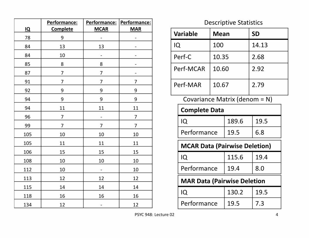
IQPerformance: Complete

Performance:MCAR

Performance: MAR

78 9 ‐ ‐

84 13 13 ‐

84 10 ‐ ‐

85 8 8 ‐

87 7 7 ‐

91 7 7 7

92 9 9 9

94 9 9 9

94 11 11 11

96 7 ‐ 7

99 7 7 7

105 10 10 10

105 11 11 11

106 15 15 15

108 10 10 10

112 10 ‐ 10

113 12 12 12

115 14 14 14

118 16 16 16

134 12 ‐ 12

Variable Mean SD

IQ 100 14.13

Perf‐C 10.35 2.68

Perf‐MCAR 10.60 2.92

Perf‐MAR 10.67 2.79

Descriptive Statistics

Covariance Matrix (denom = N)Complete Data

IQ 189.6 19.5

Performance 19.5 6.8

MCAR Data (Pairwise Deletion)

IQ 115.6 19.4


MAR Data (Pairwise Deletion

IQ 130.2 19.5


AN INTRODUCTION TO MAXIMUM LIKELIHOOD ESTIMATION


Why Estimation is Important

• In “applied” statistics courses estimation is not discussed frequently Can be very technical…very intimidating

• Estimation is of critical importance Quality and validity of estimates (and of inferences made from them)

depends on how they were obtained

• Consider an absurd example: I say the mean for IQ should be 20 – just from what I feel Do you believe me? Do you feel like reporting this result?

Estimators need a basis in reality (in statistical theory)


How Estimation Works (More or Less)• Most estimation routines do one of three things:

1. Minimize Something: Typically found with names that have “least” in the title. Forms of least squares include “Generalized”, “Ordinary”, “Weighted”, “Diagonally Weighted”, “WLSMV”, and “Iteratively Reweighted.” Typically the estimator of last resort…

2. Maximize Something: Typically found with names that have “maximum” in the title. Forms include “Maximum likelihood”, “ML”, “Residual Maximum Likelihood” (REML), “Robust ML”. Typically the gold standard of estimators.

3. Use Simulation to Sample from Something: more recent advances in simulation use resampling techniques. Names include “Bayesian Markov Chain Monte Carlo”, “Gibbs Sampling”, “Metropolis Hastings”, “Metropolis Algorithm”, and “Monte Carlo”. Used for complex models where ML is not available or for methods where prior values are needed.


Properties of Maximum Likelihood Estimators

• Provided several assumptions (“regularity conditions”) are met, maximum likelihood estimators have good statistical properties:

1. Asymptotic Consistency: as the sample size increases, the estimator converges in probability to its true value

2. Asymptotic Normality: as the sample size increases, the distribution of the estimator is normal (with variance given by “information” matrix)

3. Efficiency: No other estimator will have a smaller standard error

• Because they have such nice and well understood properties, MLEs are commonly used in statistical estimation


Maximum Likelihood: Estimates Based on Statistical Distributions

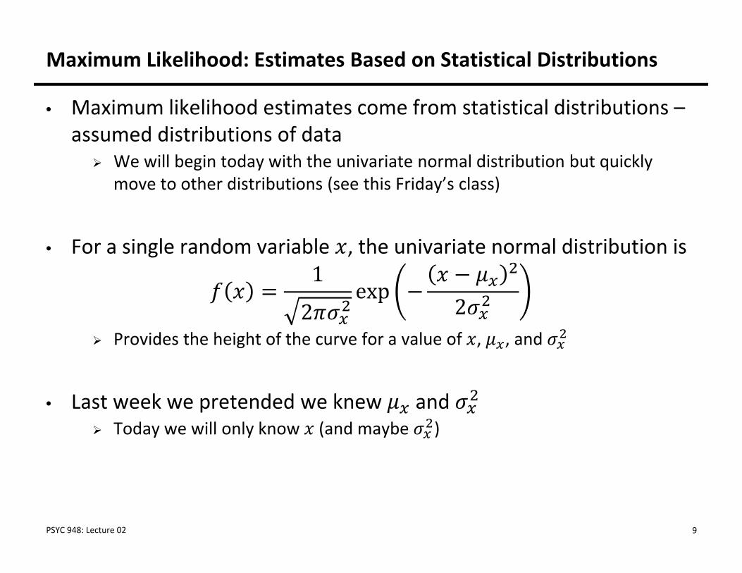
• Maximum likelihood estimates come from statistical distributions –assumed distributions of data We will begin today with the univariate normal distribution but quickly

move to other distributions (see this Friday’s class)

• For a single random variable , the univariate normal distribution is 1

2exp

2 Provides the height of the curve for a value of , , and

• Last week we pretended we knew and Today we will only know (and maybe )


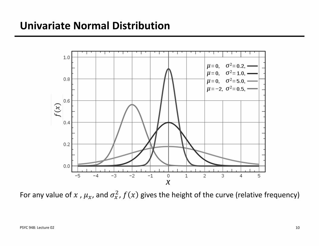
Univariate Normal Distribution


For any value of , , and , gives the height of the curve (relative frequency)

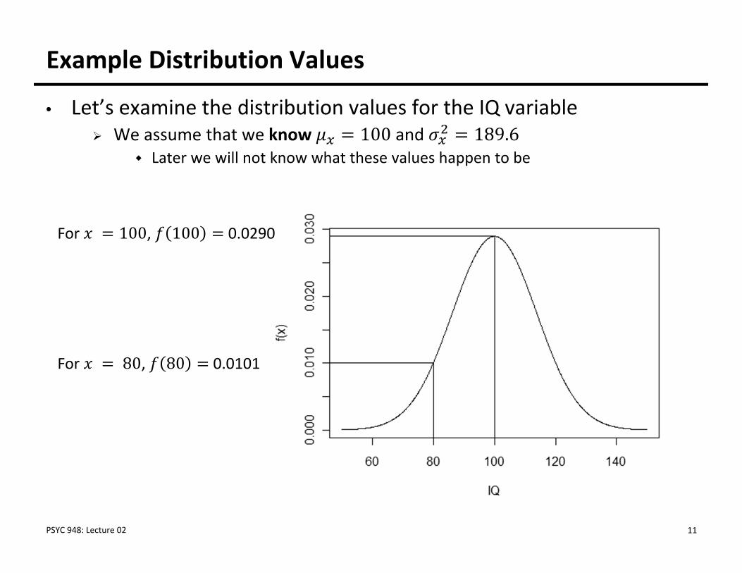
Example Distribution Values

• Let’s examine the distribution values for the IQ variable We assume that we know 100 and 189.6

Later we will not know what these values happen to be


For 80, 80 0.0101

For 100, 100 0.0290

Constructing a Likelihood Function

• Maximum likelihood estimation begins by building a likelihood function A likelihood function provides a value of a likelihood (think height of a

curve) for a set of statistical parameters

• Likelihood functions start with probability density functions (PDFs) Density functions are provided for each observation individually (marginal)

• The likelihood function for the entire sample is the function that gets used in the estimation process The sample likelihood can be thought of as a joint distribution of all the

observations, simultaneously In univariate statistics, observations are considered independent, so the

joint likelihood for the sample is constructed through a product

• To demonstrate, let’s consider the likelihood function for one observation


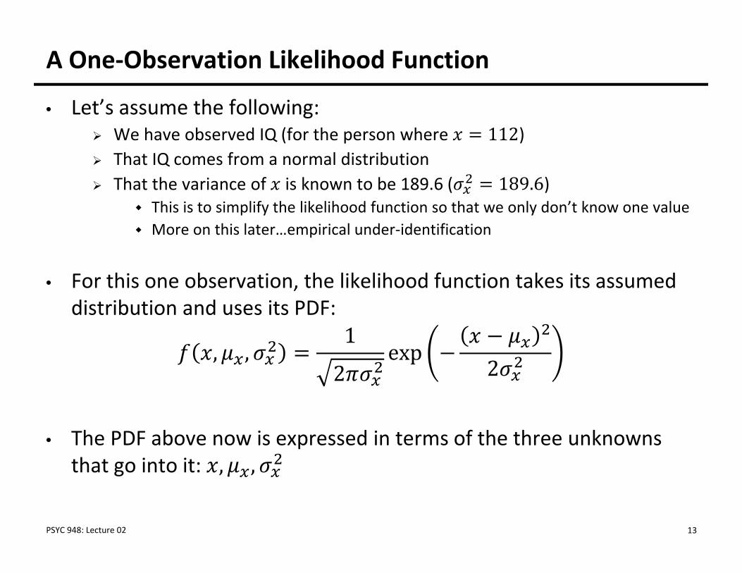
A One‐Observation Likelihood Function

• Let’s assume the following: We have observed IQ (for the person where 112) That IQ comes from a normal distribution That the variance of is known to be 189.6 ( 189.6)

This is to simplify the likelihood function so that we only don’t know one value More on this later…empirical under‐identification

• For this one observation, the likelihood function takes its assumed distribution and uses its PDF:

, ,1

2exp

2

• The PDF above now is expressed in terms of the three unknowns that go into it: , ,


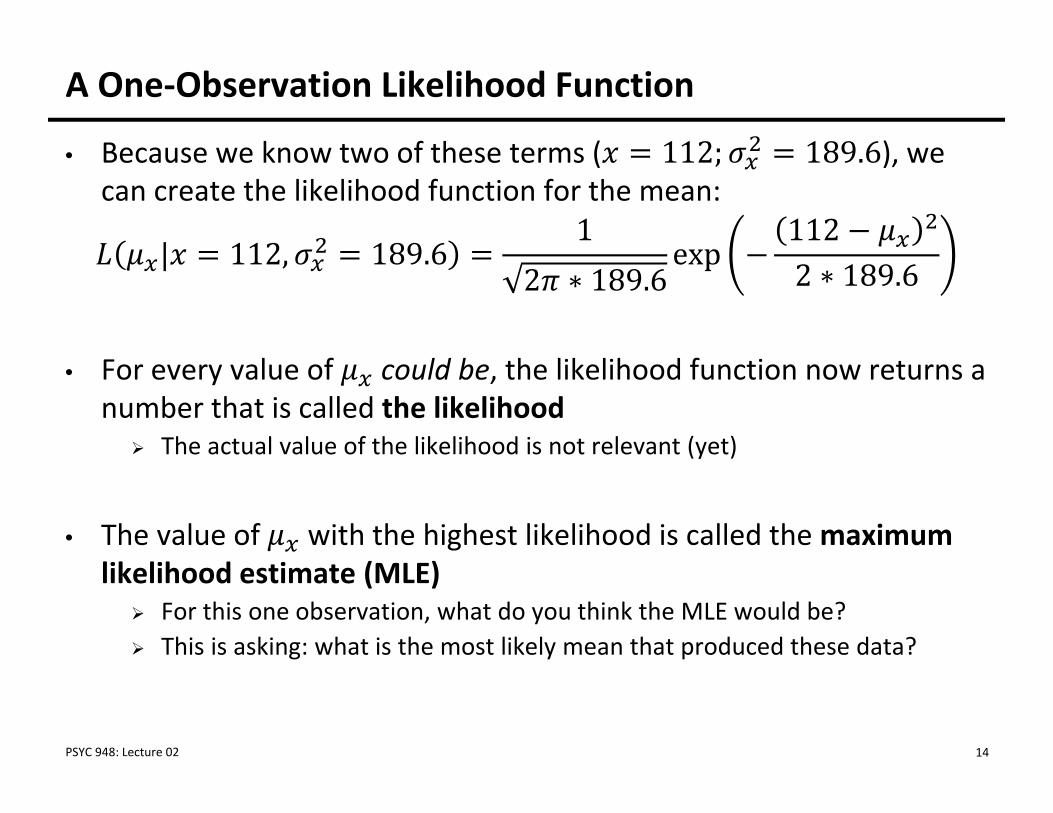
A One‐Observation Likelihood Function

• Because we know two of these terms ( 112; 189.6), we can create the likelihood function for the mean:

| 112, 189.61

2 ∗ 189.6exp

1122 ∗ 189.6

• For every value of could be, the likelihood function now returns a number that is called the likelihood The actual value of the likelihood is not relevant (yet)

• The value of with the highest likelihood is called the maximum likelihood estimate (MLE) For this one observation, what do you think the MLE would be? This is asking: what is the most likely mean that produced these data?


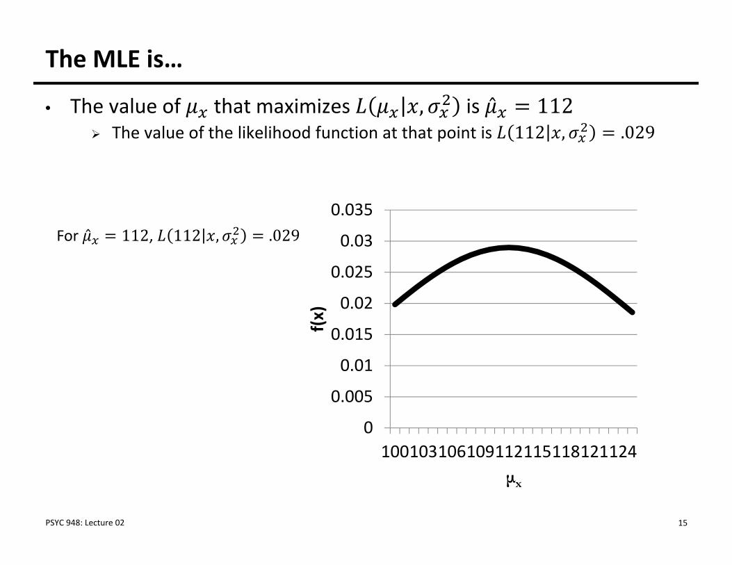
The MLE is…

• The value of that maximizes , is ̂ 112 The value of the likelihood function at that point is 112 , .029


For ̂ 112, 112 , .029

0

0.005

0.01

0.015

0.02

0.025

0.03

0.035

100103106109112115118121124

f(x)

μx

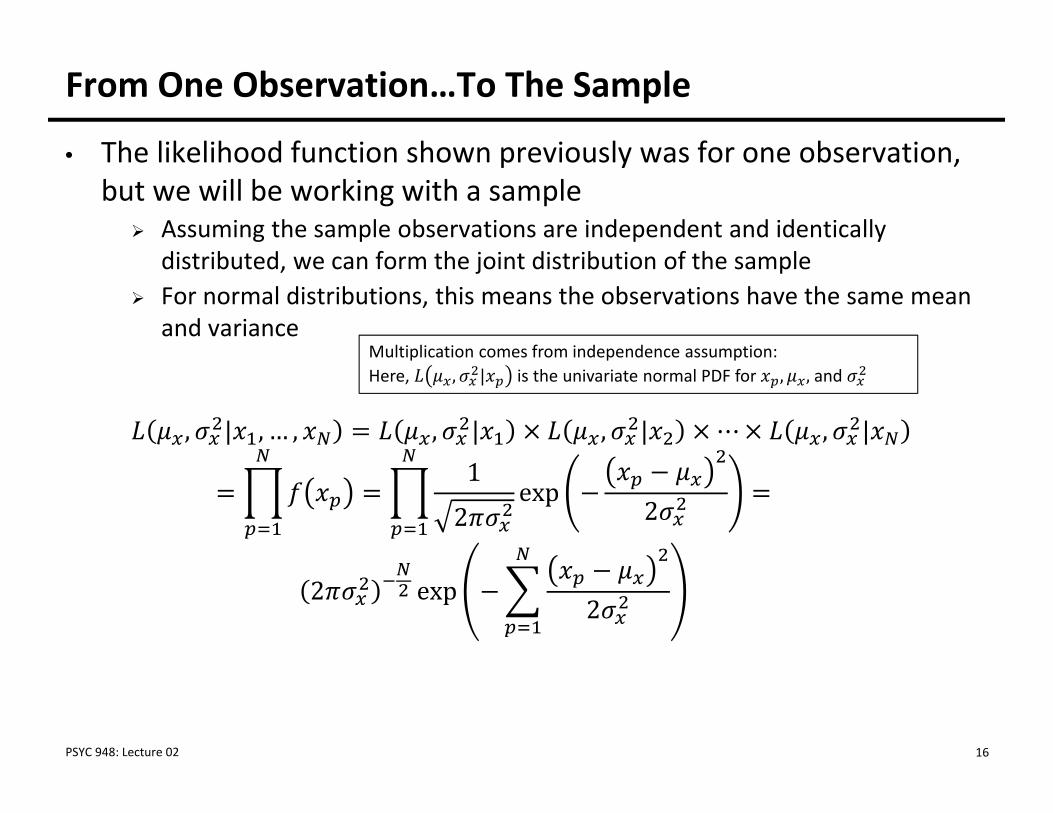
From One Observation…To The Sample

• The likelihood function shown previously was for one observation, but we will be working with a sample Assuming the sample observations are independent and identically

distributed, we can form the joint distribution of the sample For normal distributions, this means the observations have the same mean

and variance

, | , … , , | , | ⋯ , |1

2exp

2

2 exp2


Multiplication comes from independence assumption:Here, , | is the univariate normal PDF for , , and

Maximizing the Log Likelihood Function

• The process of finding the values of and that maximize the likelihood function is complicated What was shown was a grid search: trial‐and‐error process

• For relatively simple functions, we can use calculus to find the maximum of a function mathematically Problem: not all functions can give closed‐form solutions

(i.e., one solvable equation) for location of the maximum Solution: use efficient methods of searching for parameter

(i.e., Newton‐Raphson)


Standard Errors: Using the Second Derivative

• Although the estimated values of the sample mean and variance are needed, we also need the standard errors

• For MLEs, the standard errors come from the information matrix, which is found from the square root of ‐1 times the inverse matrix of second derivatives (only one value for one parameter) Second derivative gives curvature of log‐likelihood function


MAXIMUM LIKELIHOOD WITH THE MULTIVARIATE NORMAL DISTRIBUTION


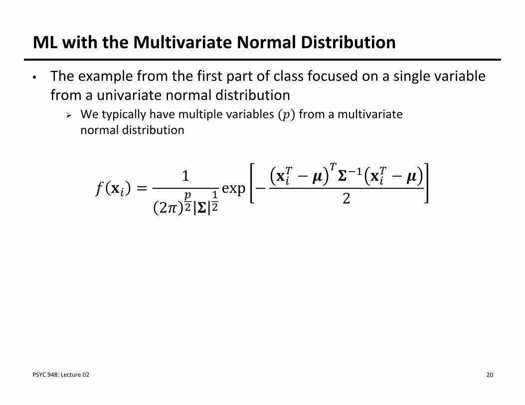
ML with the Multivariate Normal Distribution

• The example from the first part of class focused on a single variable from a univariate normal distribution We typically have multiple variables from a multivariate

normal distribution

1

2exp 2


The Multivariate Normal Distribution

1

2exp 2

• The mean vector is ⋮

• The covariance matrix is

⋯⋯

⋮ ⋮ ⋱ ⋮⋯

The covariance matrix must be non‐singular (invertible)


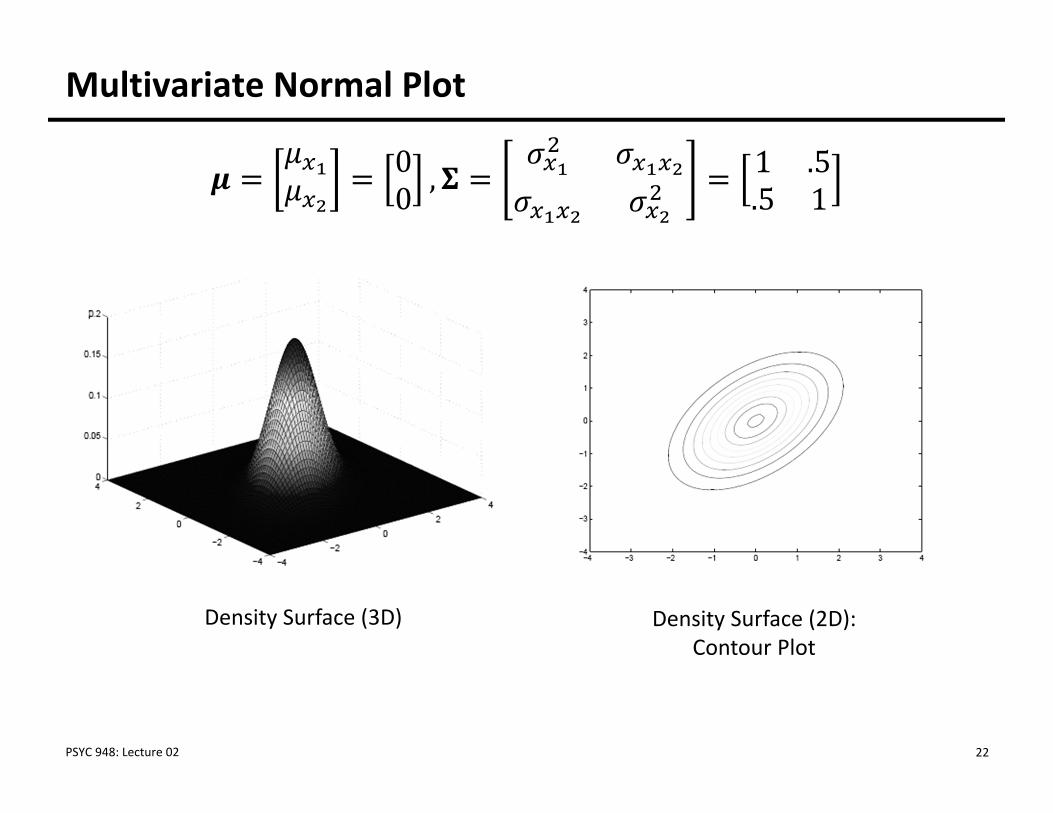
Multivariate Normal Plot

00 , 1 .5

.5 1

Density Surface (3D) Density Surface (2D): Contour Plot


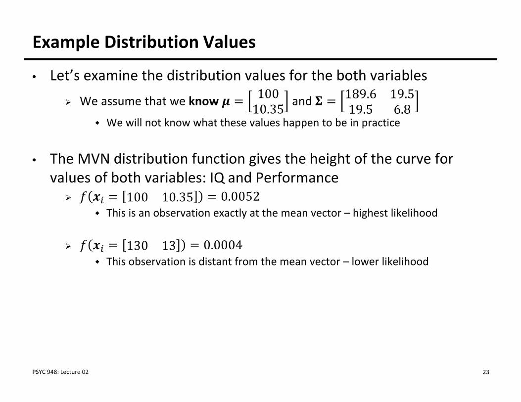
Example Distribution Values

• Let’s examine the distribution values for the both variables

We assume that we know 10010.35 and 189.6 19.5

19.5 6.8 We will not know what these values happen to be in practice

• The MVN distribution function gives the height of the curve for values of both variables: IQ and Performance 100 10.35 0.0052

This is an observation exactly at the mean vector – highest likelihood

130 13 0.0004 This observation is distant from the mean vector – lower likelihood


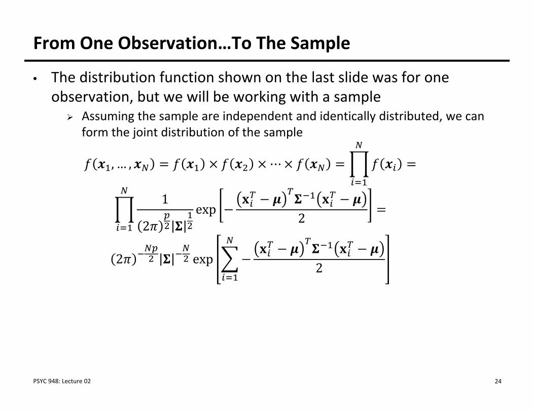
From One Observation…To The Sample

• The distribution function shown on the last slide was for one observation, but we will be working with a sample Assuming the sample are independent and identically distributed, we can

form the joint distribution of the sample

, … , ⋯

1

2exp 2

2 exp 2


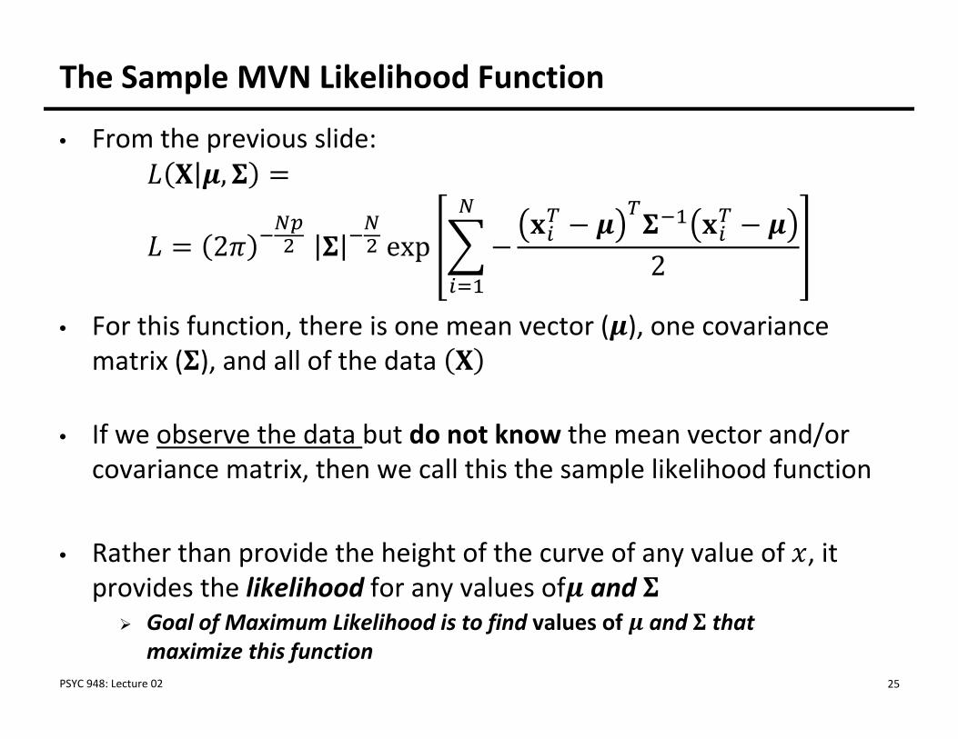
The Sample MVN Likelihood Function

• From the previous slide:,

2 exp 2

• For this function, there is one mean vector ( ), one covariance matrix ( ), and all of the data

• If we observe the data but do not know the mean vector and/or covariance matrix, then we call this the sample likelihood function

• Rather than provide the height of the curve of any value of , it provides the likelihood for any values of and Goal of Maximum Likelihood is to find values of and that

maximize this functionPSYC 948: Lecture 02 25

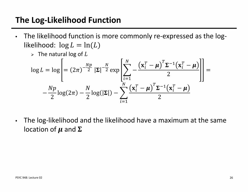
The Log‐Likelihood Function

• The likelihood function is more commonly re‐expressed as the log‐likelihood: log ln The natural log of

log log 2 exp 2

2 log 2 2 log 2

• The log‐likelihood and the likelihood have a maximum at the same location of and


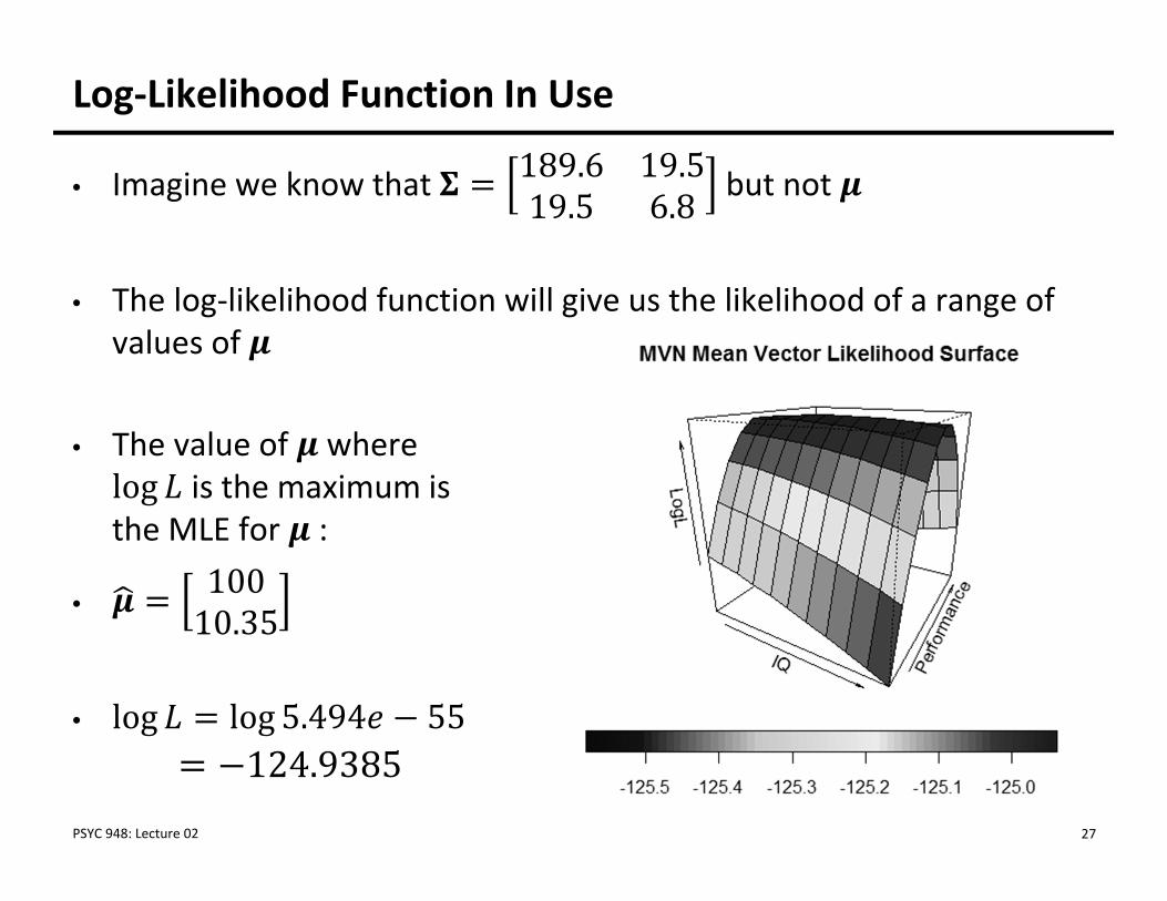
• Imagine we know that 189.6 19.519.5 6.8 but not

• The log‐likelihood function will give us the likelihood of a range of values of

• The value of where log is the maximum is the MLE for :

•10010.35

• log log 5.494 55

Log‐Likelihood Function In Use


Finding MLEs In Practice

• Most likelihood functions do not have closed form estimates Iterative algorithms must be used to find estimates

• Iterative algorithms begin at a location of the log‐likelihood surface and then work to find the peak Each iteration brings estimates closer to the maximum Change in log‐likelihood from one iteration to the next should be small

• If models have latent (random) components, then these components are “marginalized” – removed from equation Called Marginal Maximum Likelihood

• Once the algorithm finds the peak, then the estimates used to find the peak are called the MLEs And the information matrix is obtained providing standard errors for each


MAXIMUM LIKELIHOOD BY MVN: USING MPLUS FOR ESTIMATION


Using MVN Likelihoods in MPlus

• In Mplus, the default assumption for variables is a linear (mixed) models procedure that uses (full information) ML with the multivariate normal distribution Full Information = All Data Contribute

• You can use Mplus to do analyses for all sorts of linear models including: MANOVA Repeated Measures ANOVA Multilevel models/Hierarchical Linear Models (Some) Factor Models

• The MVN is what we will use for the first part of this class Later, we will work with distributions for categorical outcomes


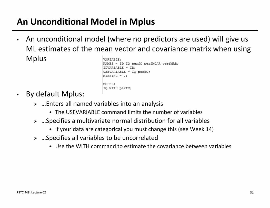
• An unconditional model (where no predictors are used) will give us ML estimates of the mean vector and covariance matrix when using Mplus

• By default Mplus: …Enters all named variables into an analysis

The USEVARIABLE command limits the number of variables …Specifies a multivariate normal distribution for all variables

If your data are categorical you must change this (see Week 14) …Specifies all variables to be uncorrelated

Use the WITH command to estimate the covariance between variables

An Unconditional Model in Mplus


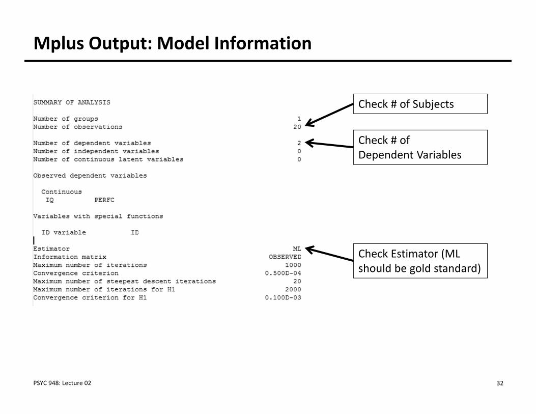
Mplus Output: Model Information

PSYC 948: Lecture 02

Check # of Subjects

Check # of Dependent Variables

Check Estimator (ML should be gold standard)

32

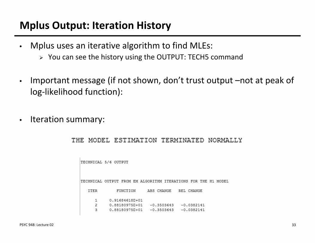
Mplus Output: Iteration History

• Mplus uses an iterative algorithm to find MLEs: You can see the history using the OUTPUT: TECH5 command

• Important message (if not shown, don’t trust output –not at peak of log‐likelihood function):

• Iteration summary:


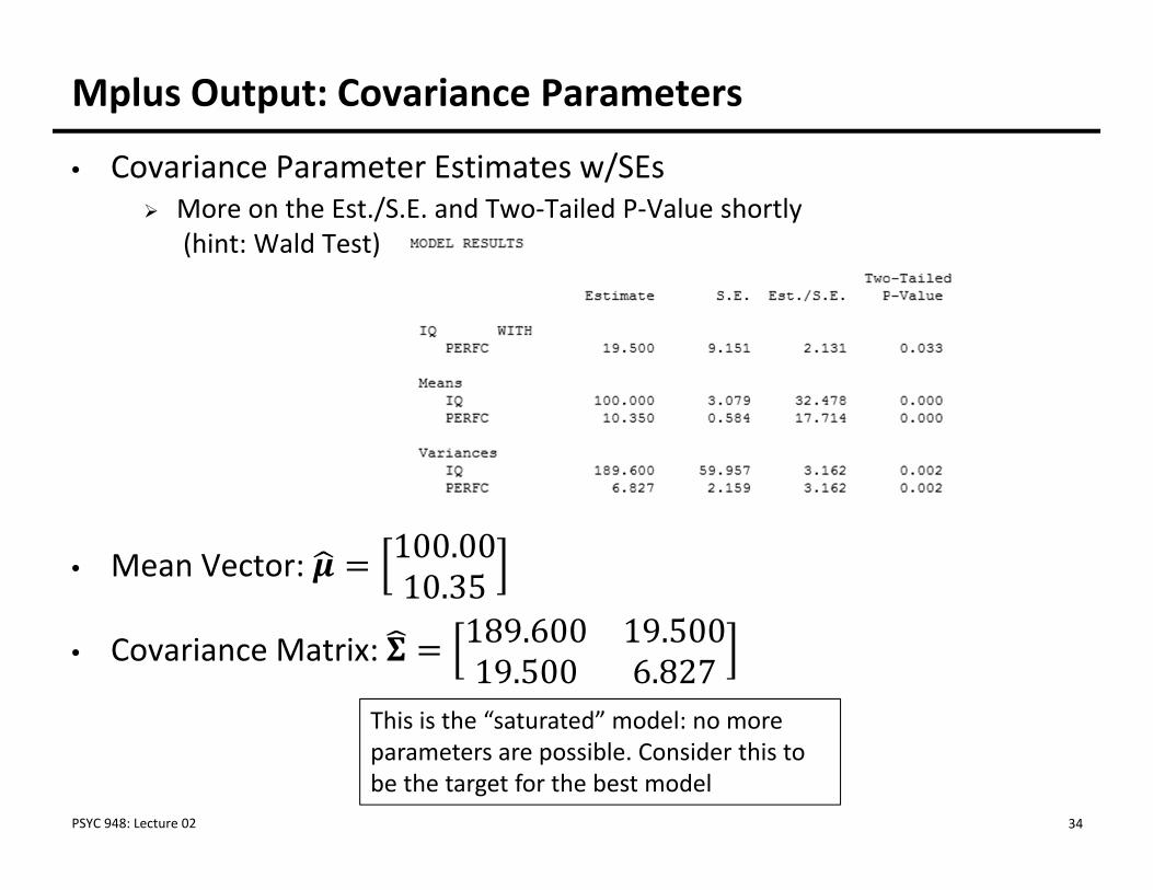
Mplus Output: Covariance Parameters

• Covariance Parameter Estimates w/SEs More on the Est./S.E. and Two‐Tailed P‐Value shortly

(hint: Wald Test)

• Mean Vector: 100.0010.35

• Covariance Matrix: 189.600 19.50019.500 6.827


This is the “saturated” model: no more parameters are possible. Consider this to be the target for the best model

USEFUL PROPERTIES OF MAXIMUM LIKELIHOOD ESTIMATES


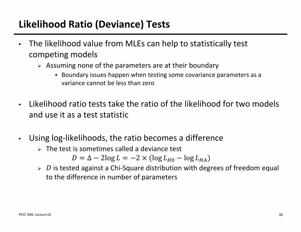
Likelihood Ratio (Deviance) Tests

• The likelihood value from MLEs can help to statistically test competing models Assuming none of the parameters are at their boundary

Boundary issues happen when testing some covariance parameters as a variance cannot be less than zero

• Likelihood ratio tests take the ratio of the likelihood for two models and use it as a test statistic

• Using log‐likelihoods, the ratio becomes a difference The test is sometimes called a deviance test

Δ 2log 2 log log is tested against a Chi‐Square distribution with degrees of freedom equal

to the difference in number of parameters


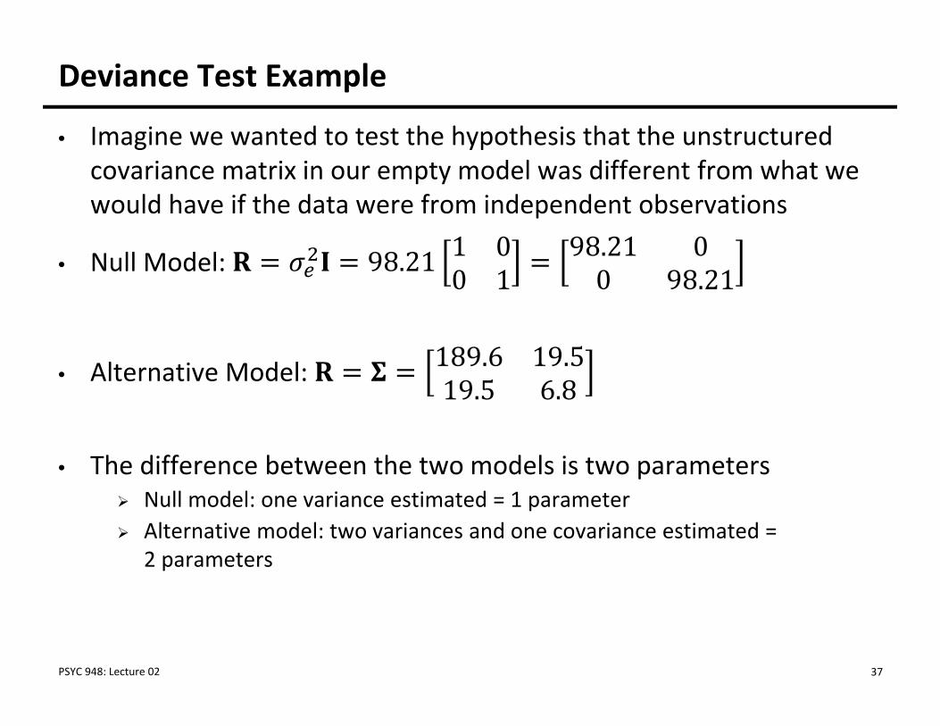
Deviance Test Example

• Imagine we wanted to test the hypothesis that the unstructured covariance matrix in our empty model was different from what we would have if the data were from independent observations

• Null Model: 98.21 1 00 1

98.21 00 98.21

• Alternative Model: 189.6 19.519.5 6.8

• The difference between the two models is two parameters Null model: one variance estimated = 1 parameter Alternative model: two variances and one covariance estimated =

2 parameters


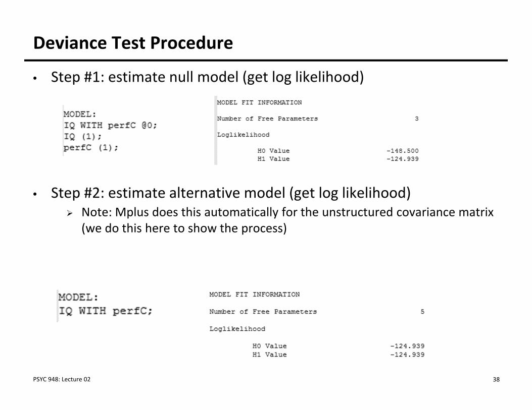
Deviance Test Procedure

• Step #1: estimate null model (get log likelihood)

• Step #2: estimate alternative model (get log likelihood) Note: Mplus does this automatically for the unstructured covariance matrix

(we do this here to show the process)


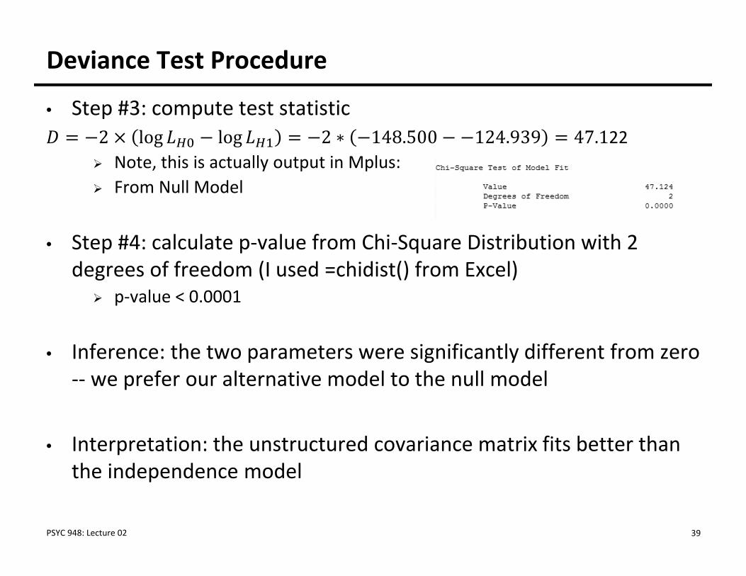
Deviance Test Procedure

• Step #3: compute test statistic2 log log 2 ∗ 148.500 124.939 47.122 Note, this is actually output in Mplus: From Null Model

• Step #4: calculate p‐value from Chi‐Square Distribution with 2 degrees of freedom (I used =chidist() from Excel) p‐value < 0.0001

• Inference: the two parameters were significantly different from zero ‐‐ we prefer our alternative model to the null model

• Interpretation: the unstructured covariance matrix fits better than the independence model


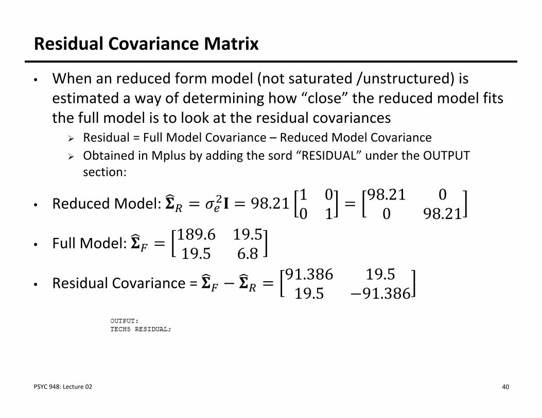
Residual Covariance Matrix

• When an reduced form model (not saturated /unstructured) is estimated a way of determining how “close” the reduced model fits the full model is to look at the residual covariances Residual = Full Model Covariance – Reduced Model Covariance Obtained in Mplus by adding the sord “RESIDUAL” under the OUTPUT

section:

• Reduced Model: 98.21 1 00 1

98.21 00 98.21

• Full Model: 189.6 19.519.5 6.8

• Residual Covariance = 91.386 19.519.5 91.386


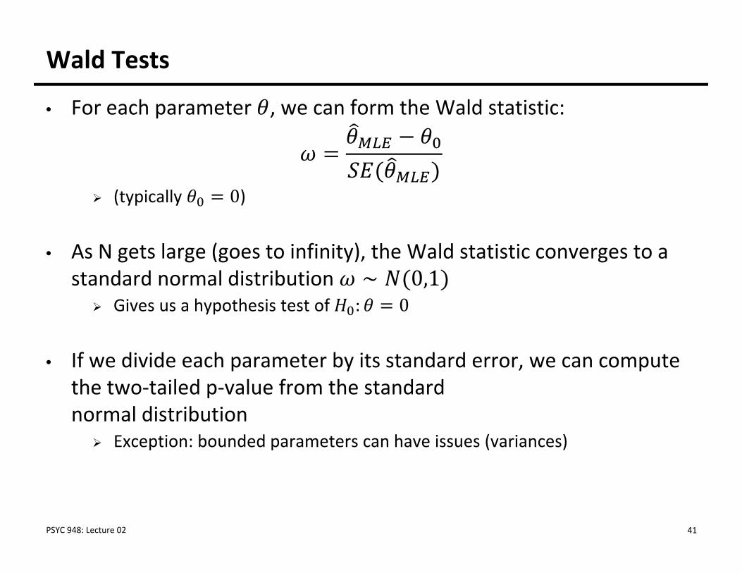
Wald Tests

• For each parameter , we can form the Wald statistic:

(typically 0)

• As N gets large (goes to infinity), the Wald statistic converges to a standard normal distribution ∼ 0,1 Gives us a hypothesis test of : 0

• If we divide each parameter by its standard error, we can compute the two‐tailed p‐value from the standard normal distribution Exception: bounded parameters can have issues (variances)


Wald Test Example

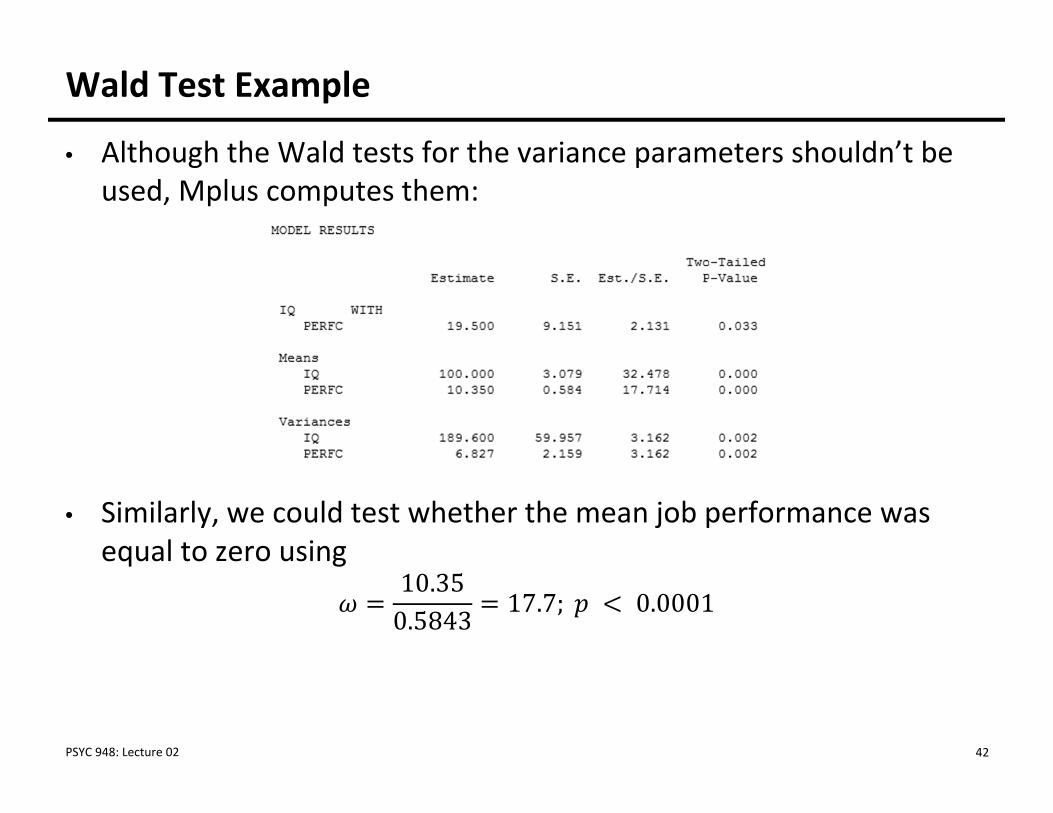
• Although the Wald tests for the variance parameters shouldn’t be used, Mplus computes them:

• Similarly, we could test whether the mean job performance was equal to zero using

10.350.5843 17.7; 0.0001


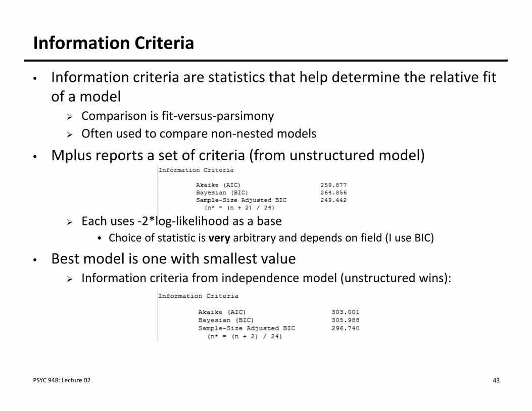
• Information criteria are statistics that help determine the relative fit of a model Comparison is fit‐versus‐parsimony Often used to compare non‐nested models

• Mplus reports a set of criteria (from unstructured model)

Each uses ‐2*log‐likelihood as a base Choice of statistic is very arbitrary and depends on field (I use BIC)

• Best model is one with smallest value Information criteria from independence model (unstructured wins):

Information Criteria


ROBUST ML IN CFA/SEM


Robust Estimation: The Basics

• Robust estimation in ML still assumes the data follow a multivariate normal distribution But that the data have more or less kurtosis than would otherwise be

common in a normal distribution

• Kurtosis: measure of the shape of the distribution From Greek word for bulging Can be estimated for data (either marginally for each item or jointly across

all items)

• The degree of kurtosis in a data set is related to how incorrect the log‐likelihood value will be Leptokurtic data (too‐fat tails): inflated, SEs too small Platykurtic data (too‐thin tails): depressed, SEs too large


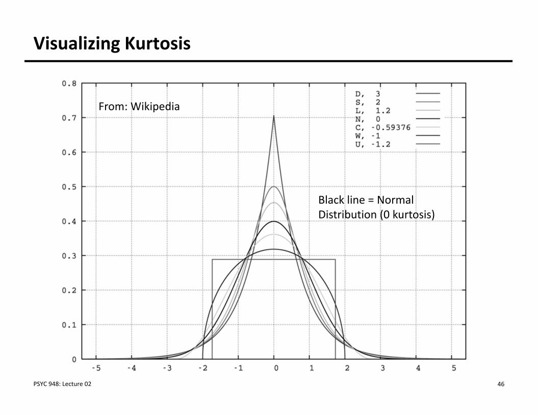
Visualizing Kurtosis

From: Wikipedia

Black line = Normal Distribution (0 kurtosis)


Robust ML for Non‐Normality in Mplus: MLR

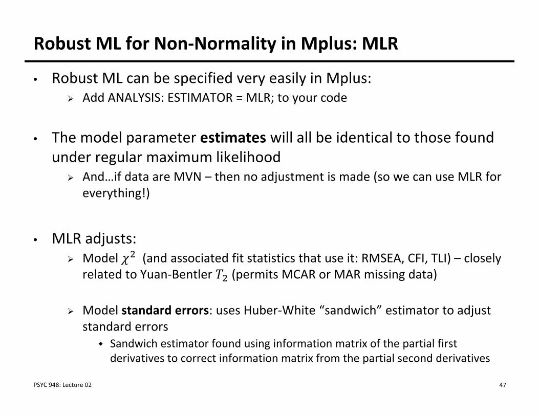
• Robust ML can be specified very easily in Mplus: Add ANALYSIS: ESTIMATOR = MLR; to your code

• The model parameter estimates will all be identical to those found under regular maximum likelihood And…if data are MVN – then no adjustment is made (so we can use MLR for

everything!)

• MLR adjusts: Model (and associated fit statistics that use it: RMSEA, CFI, TLI) – closely

related to Yuan‐Bentler (permits MCAR or MAR missing data)

Model standard errors: uses Huber‐White “sandwich” estimator to adjust standard errors Sandwich estimator found using information matrix of the partial first derivatives to correct information matrix from the partial second derivatives


Adjusted Model Fit Statistics

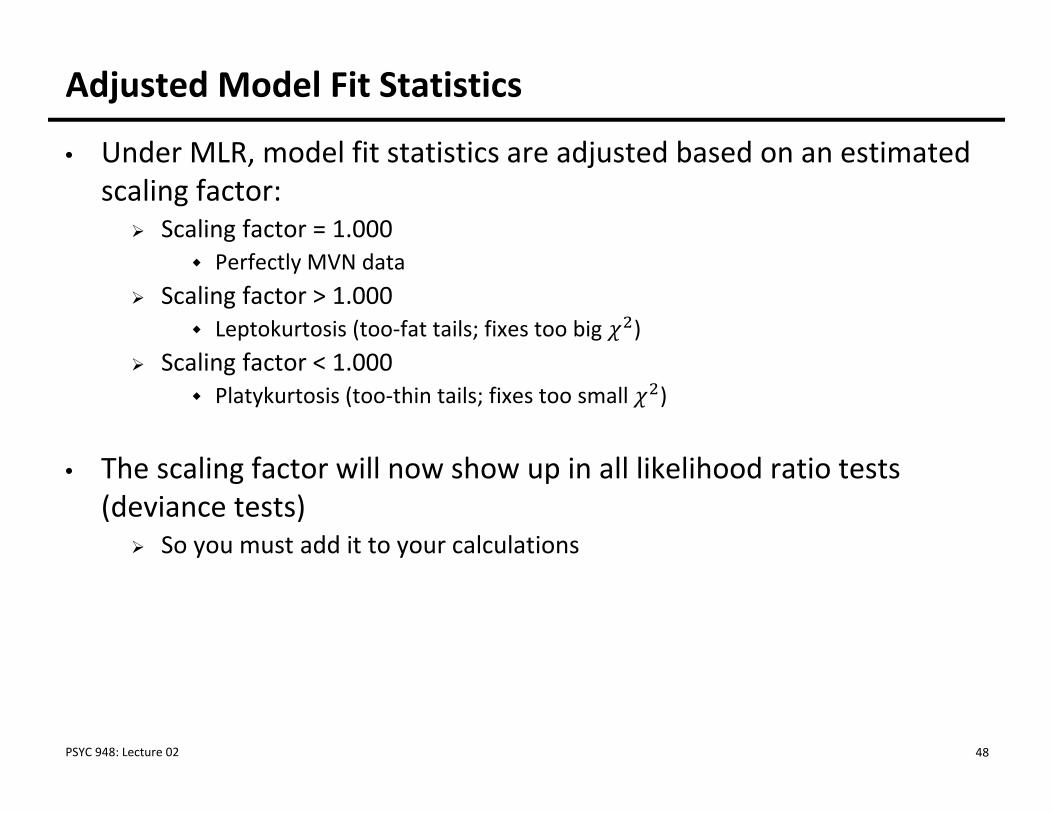
• Under MLR, model fit statistics are adjusted based on an estimated scaling factor: Scaling factor = 1.000

Perfectly MVN data Scaling factor > 1.000

Leptokurtosis (too‐fat tails; fixes too big ) Scaling factor < 1.000

Platykurtosis (too‐thin tails; fixes too small )

• The scaling factor will now show up in all likelihood ratio tests (deviance tests) So you must add it to your calculations


Adjusted Standard Errors

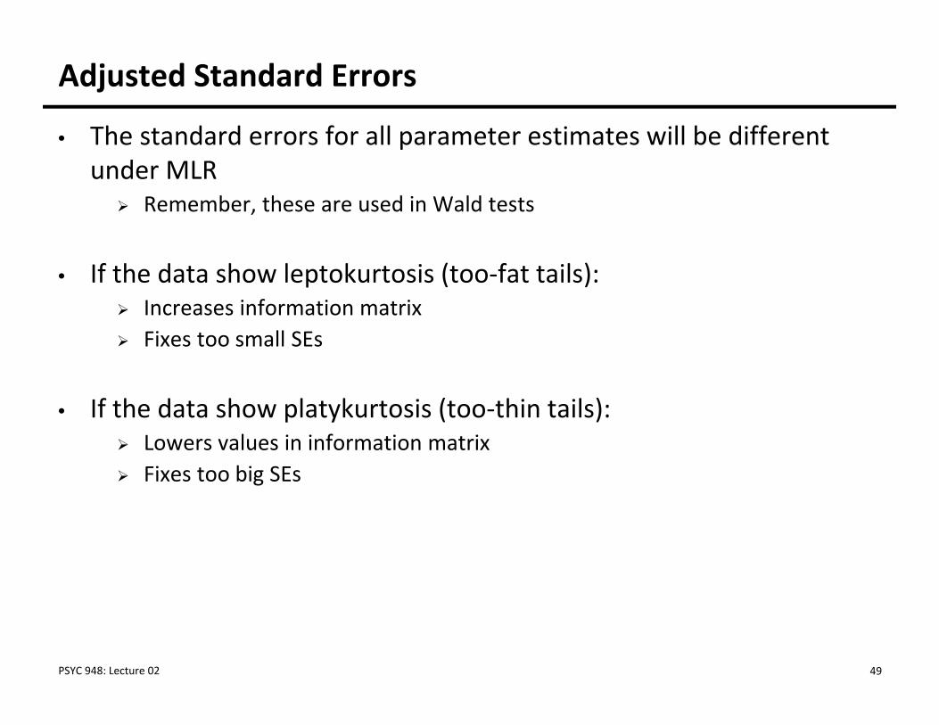
• The standard errors for all parameter estimates will be different under MLR Remember, these are used in Wald tests

• If the data show leptokurtosis (too‐fat tails): Increases information matrix Fixes too small SEs

• If the data show platykurtosis (too‐thin tails): Lowers values in information matrix Fixes too big SEs


Data Analysis Example with MLR

• To demonstrate, we will revisit our analysis of the example data for today’s class using MLR

• So far, we have estimated two models: Saturated model Independence model

• The results of the two analyses (ML v. MLR) will be compared

• Because MLR is something does not affect our results if we have MVN data, we should have been using MLR all along


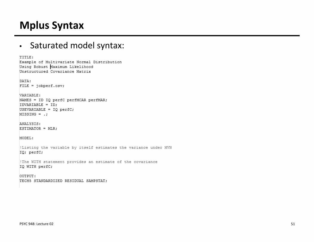
Mplus Syntax

• Saturated model syntax:


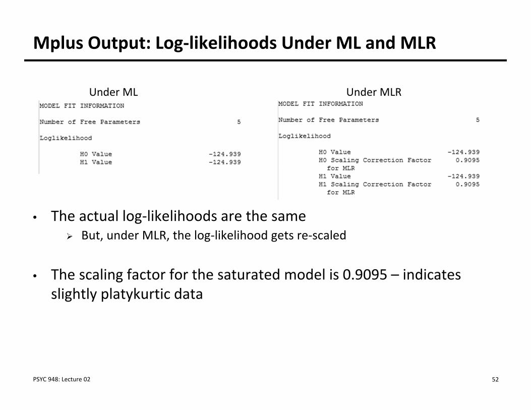
Mplus Output: Log‐likelihoods Under ML and MLR

• The actual log‐likelihoods are the same But, under MLR, the log‐likelihood gets re‐scaled

• The scaling factor for the saturated model is 0.9095 – indicates slightly platykurtic data

Under ML Under MLR


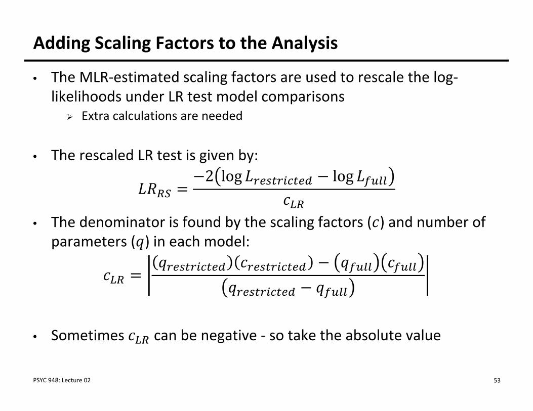
Adding Scaling Factors to the Analysis

• The MLR‐estimated scaling factors are used to rescale the log‐likelihoods under LR test model comparisons Extra calculations are needed

• The rescaled LR test is given by:2 log log

• The denominator is found by the scaling factors ( ) and number of parameters ( ) in each model:

• Sometimes can be negative ‐ so take the absolute value


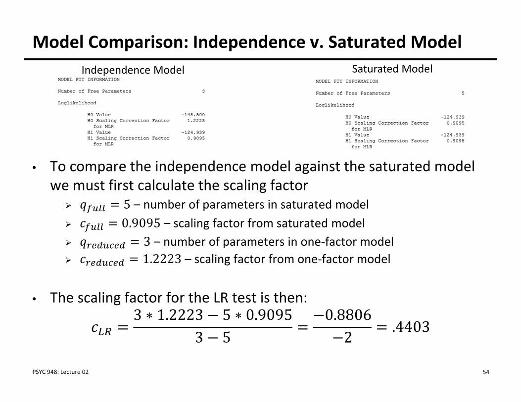
Model Comparison: Independence v. Saturated Model

• To compare the independence model against the saturated model we must first calculate the scaling factor 5 – number of parameters in saturated model 0.9095 – scaling factor from saturated model 3 – number of parameters in one‐factor model 1.2223 – scaling factor from one‐factor model

• The scaling factor for the LR test is then:3 ∗ 1.2223 5 ∗ 0.9095

3 50.88062 .4403


Saturated ModelIndependence Model

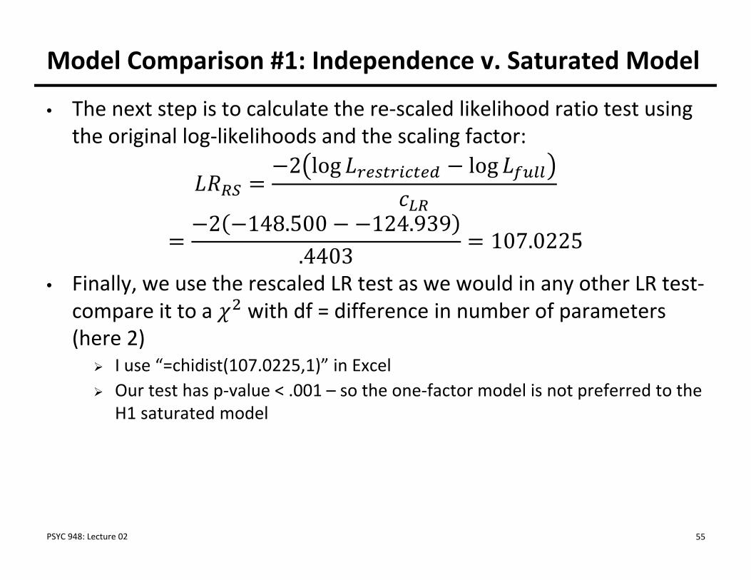
Model Comparison #1: Independence v. Saturated Model

• The next step is to calculate the re‐scaled likelihood ratio test using the original log‐likelihoods and the scaling factor:

2 log log

2 148.500 124.939.4403 107.0225

• Finally, we use the rescaled LR test as we would in any other LR test‐compare it to a with df = difference in number of parameters (here 2) I use “=chidist(107.0225,1)” in Excel Our test has p‐value < .001 – so the one‐factor model is not preferred to the

H1 saturated model


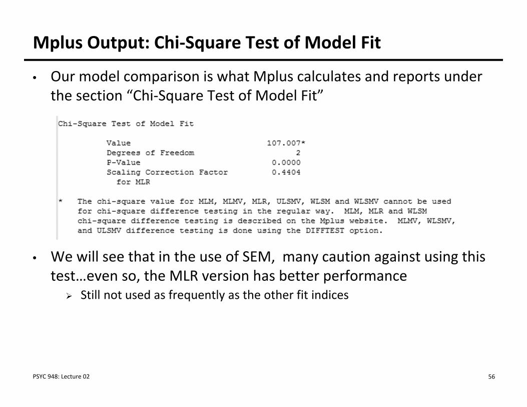
Mplus Output: Chi‐Square Test of Model Fit

• Our model comparison is what Mplus calculates and reports under the section “Chi‐Square Test of Model Fit”

• We will see that in the use of SEM, many caution against using this test…even so, the MLR version has better performance Still not used as frequently as the other fit indices


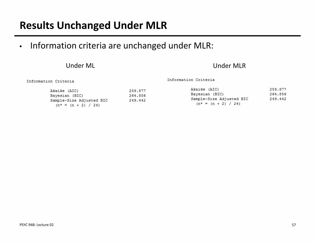
Results Unchanged Under MLR

• Information criteria are unchanged under MLR:

Under ML Under MLR


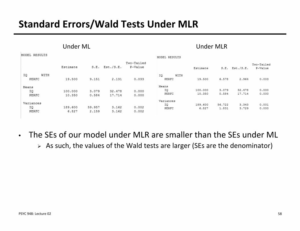
Standard Errors/Wald Tests Under MLR

• The SEs of our model under MLR are smaller than the SEs under ML As such, the values of the Wald tests are larger (SEs are the denominator)

Under ML Under MLR


MLR: The Take‐Home Point

• If you feel you have continuous data that are (tenuously) normally distributed, use MLR Any time you use SEM/CFA/Path Analysis as we have to this point In general, likert‐type items with 5 or more categories are treated this way If data aren’t/cannot be considered normal we should still use different

distributional assumptions

• If data truly are MVN, then MLR doesn’t adjust anything

• If data are not MVN (but are still continuous), then MLR adjusts the important inferential portions of the results


WRAPPING UP


Wrapping Up

• Today was a refresher course on ML and “Robust” ML estimation These topics will come back to us each week – so lots of opportunity

for practice

• These topics are important when using Mplus as there are quite a few different estimators in the package ML is not always the default

• Homework #2: available on our website – due next Wednesday (January 23rd) at 11:59am


maximum likelihood and robust maximum likelihood

Documents