may 2004motion/optic flow1 motion field and optical flow ack, for the slides: professor yuan-fang...

May 2004 Motion/Optic Flow 1

Motion Field and Optical Flow

Ack, for the slides:

Professor Yuan-Fang WangProfessor Octavia Camps


Motion Field and Optical Flow

• So far, algorithms deal with a single, static image

• In real world, a static pattern is a rarity, continuous motion and change are the rule

• Human eyes are well-equipped to take advantage of motion or change in an image sequence.– In our discussions, an image sequence is a discrete set of N

images, taken at discrete time instants (may or may not be uniformly spaced in time).

• Image changes are due to the relative motion between the camera and the scene (illumination being constant).


Example

• Ullman’s concentric counter-rotating cylinder experiment

• Two concentric cylinders of different radii

• W. a random dot pattern on both surfaces (cylinder surfaces and boundaries are not displayed)

• Stationary: not able to tell them apart

• Counter-rotating: structures apparent


• Motion helps in– segmentation (two structures)

– identification (two cylinders)

Example (cont.)


General Scenario

Possibilities:• camera moving, stationary scene• camera stationary, moving objects• both camera and scene moving


Visual Motion

• Allows us to compute useful properties of the 3D world, with very little knowledge.

• Example: Time to collision


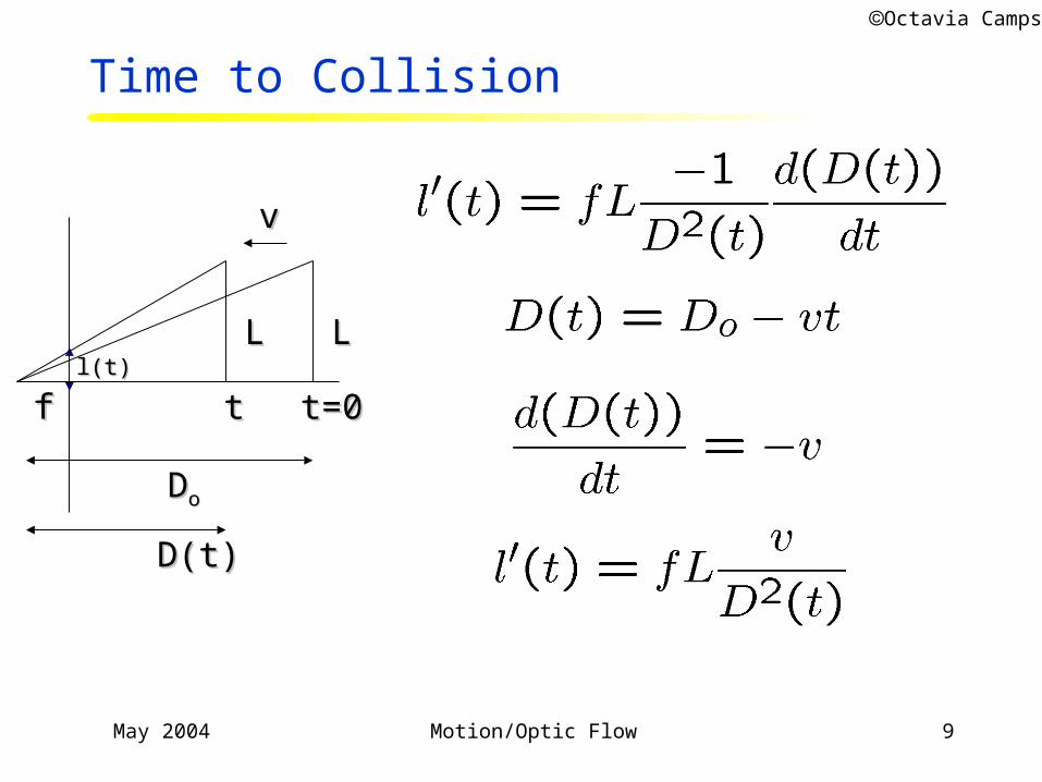
Time to Collision

ff

LL

vv

LL

DDoo

l(t)l(t)

An object of heightAn object of height L L moves with moves with

constant velocity constant velocity v:v:•At time At time t=0t=0 the object is at: the object is at:

• D(0) = DD(0) = Doo

•At time At time tt it is at it is at

•D(t) = DD(t) = Doo – vt – vt

•It will crash with the camera at It will crash with the camera at

time:time:

• D(D() = D) = Doo – v – v = 0 = 0

• = D= Doo/v/v

t=0t=0tt

D(t)D(t)

Octavia Camps


Time to Collision

ff

LL

vv

LL

DDoo

l(t)l(t)

t=0t=0tt

D(t)D(t)

The image of the object has size The image of the object has size

l(t):l(t):

Taking derivative wrt time:Taking derivative wrt time:

Octavia Camps


Time to Collision

ff

LL

vv

LL

DDoo

l(t)l(t)

t=0t=0tt

D(t)D(t)

Octavia Camps


Time to Collision

ff

LL

vv

LL

DDoo

l(t)l(t)

t=0t=0tt

D(t)D(t)

And their ratio is:And their ratio is:

Octavia Camps


Time to Collision

ff

LL

vv

LL

DDoo

l(t)l(t)

t=0t=0tt

D(t)D(t)

And And time to collisiontime to collision::

Can be Can be directly directly measured measured from from imageimage

Can be found, without knowing Can be found, without knowing LL or or DDoo or or vv !! !!

Octavia Camps


Comparison between Motion Analysis and Stereo

• Stereo: Two or more frames

• Motion: N frames

baselinebaseline

timetime

•The baseline is usually The baseline is usually

larger in stereo than in larger in stereo than in

motion:motion:•Motion disparities tend Motion disparities tend

to be smallerto be smaller

•Stereo images are Stereo images are

taken at the same time:taken at the same time:•Motion disparities can Motion disparities can

be due to scene motionbe due to scene motion•There can be more than There can be more than

1 transformation btw 1 transformation btw

framesframes

Octavia Camps


Why Multitude of Formulations?

• The camera can – be stationary– execute simple translational motion– undergo general motion with both translation and rotation

• The object(s) can – be stationary

– execute simple 2D motion parallel to the image plane

– undergo general motion with both 3D translation and rotation


Why Multitude of Formulations? (cont.)

• There may be multiple moving and stationary objects in a scene

• The camera motion may be known or unknown

• The shape of the object may be known or unknown

• The motion of the object may be known or unknown

• etc. etc. ...


Motion Field (MF)

• The MF assigns a velocity vector to each pixel in the image.

• These velocities are INDUCED by the RELATIVE MOTION btw the camera and the 3D scene

• The MF can be thought as the projection of the 3D velocities on the image plane.

Octavia Camps


MF Estimation

We will use the apparent motion of brightness patterns observed in an image sequence. This motion is called OPTICAL FLOW (OF)

Octavia Camps


MF OF

Consider a smooth, lambertian, uniform sphere rotating around a diameter, in front of a camera:

–MF 0 since the points on the sphere are moving–OF = 0 since there are no moving patterns in the images

3D3D ImageImage

Octavia Camps


MF OF

Consider a still, smooth, specular, uniform sphere, in front of a stationary camera and a moving light source:

–MF 0 since the points on the sphere are not moving–OF 0 since there is a moving pattern in the images

3D3D Image1Image1 Image2Image2

Octavia Camps


Approximation of the MF

Never the less, keeping in mind that MF OF, we will assume that the apparent brightness of moving objects remain constant and hence we will estimate OF instead (since MF cannot really be observed!)

Octavia Camps


Brightness Constancy Equation

• Let P be a moving point in 3D:– At time t, P has coords (X(t),Y(t),Z(t))

– Let p=(x(t),y(t)) be the coords. of its image at time t.

– Let I(x(t),y(t),t) be the brightness at p at time t.

• Brightness Constancy Assumption:– As P moves over time, I(x(t),y(t),t) remains constant.

Octavia Camps


Approaches

• Feature based– tracking significant image features across multiple frames

– sparse motion vectors at few feature points

• Flow based– matching intensity profiles across multiple frames

– dense motion fields

• Correlation based– parametric model

• Spatial-temporal filtering– biology-motivated approach


Feature-Based Tracking

• Image features (patterns) w. unique and invariant intensity profiles

• Detect such patterns (corners, edges, etc.) in sequences of images

• Track their motion over time


Example

Computing Optical Flowt t t+δ t t+ 2δ

( , )u v

I x y t( , , ) I x u t y v t t t( , , )+ + +δ δ δ I x u t y v t t t( , , )+ + +2 2 2δ δ δ= =I x u t y v t t t

I x y tI

xu t

I

yv t

I

tt high order terms

I

xu t

I

yv t

I

tt

I

xu

I

yv

I

t

I

x

I

yu v

I

t

( , , )

( , , )

( , ) ( , )

+ + +

= + + + + − −

+ + =

+ + =

⋅ =−

δ δ δ∂∂

δ ∂∂

δ ∂∂

δ

∂∂

δ ∂∂

δ ∂∂

δ

∂∂

∂∂

∂∂

∂∂

∂∂

∂∂

0

0


• Physical Interpretation

• Q: what is

• A: image brightness gradient direction– known (spatial derivatives)

• Q: what is

• A: local motion vector – unknown

• Q: what is

• A: change of brightness at a location w.r.t time – known (temporal derivative)

( , ) ( , )∂∂

∂∂

∂∂

Ix

Iy

u vIt

⋅ =−

( , )?∂∂

∂∂

Ix

Iy

( , )?u v

∂∂

I

t?

Optical Flow Constraint Equation


no spatial change in brightness induce no temporal change in brightness no discernible motion

motion perpendicular to local gradient induce no temporal change in brightness no discernible motion

motion in the direction of local gradient induce temporal change in brightness discernible motion

only the motion component in the direction of local gradient induce temporal change in brightness discernible motion

Optical Flow Constraint


The aperture problem

The Image Brightness Constancy Assumption The Image Brightness Constancy Assumption only provides the OF component in the direction only provides the OF component in the direction of the spatial image gradientof the spatial image gradient

Octavia Camps


Difficulty

• One equation with two unknowns

• Aperture problem– spatial derivatives use only a few adjacent pixels (limited aperture

and visibility)

– many combinations of (u,v) will satisfy the equation

Constraint line

u

v


intensity gradient is zerono constraints on (u,v)interpolated from other places

intensity gradient is nonzero but is constantone constraints on (u,v)only the component along the gradientare recoverable

intensity gradient is nonzeroand changingmultiple constraints on (u,v)motion recoverable

( , ) ( , )0 0 0⋅ =u v

( , ) ( , )∂∂

∂∂

∂∂

Ix

Iy

u vIt

⋅ =−

( , ) ( , )

( , ) ( , )

( , )

( , )

∂∂

∂∂

∂∂

∂∂

∂∂

∂∂

Ix

Iy

u vIt

Ix

Iy

u vIt

x y

x y

1 1

2 2

1 1

2 2

⋅ =−

⋅ =−


Temporal coherency

t t t+δ t t+ 2δ

( , )u v( , )u v

( , ) ( , )∂∂

∂∂

∂∂

Ix

Iy

u vIt

⋅ =− ( , ) ( , )∂∂

∂∂

∂∂

Ix

Iy

u vIt

⋅ =−

• Caveat:– (u,v) must stay the same across several frames– scenes highly textured – (u,v) at the same location actually refers to

different object points


Results


Spatial-Temporal Filtering

• Motivation – It was known (Hubel and Wisel, “Receptive fields of single neurons in the cat’s striate

cortex”, 1959) that simple cells in visual cortex act like bar or edge detectors

– They function like linear filters: their receptive field profiles represent a weighting function (spatial impulse response of a linear system)

– However, their response is not temporally dependent


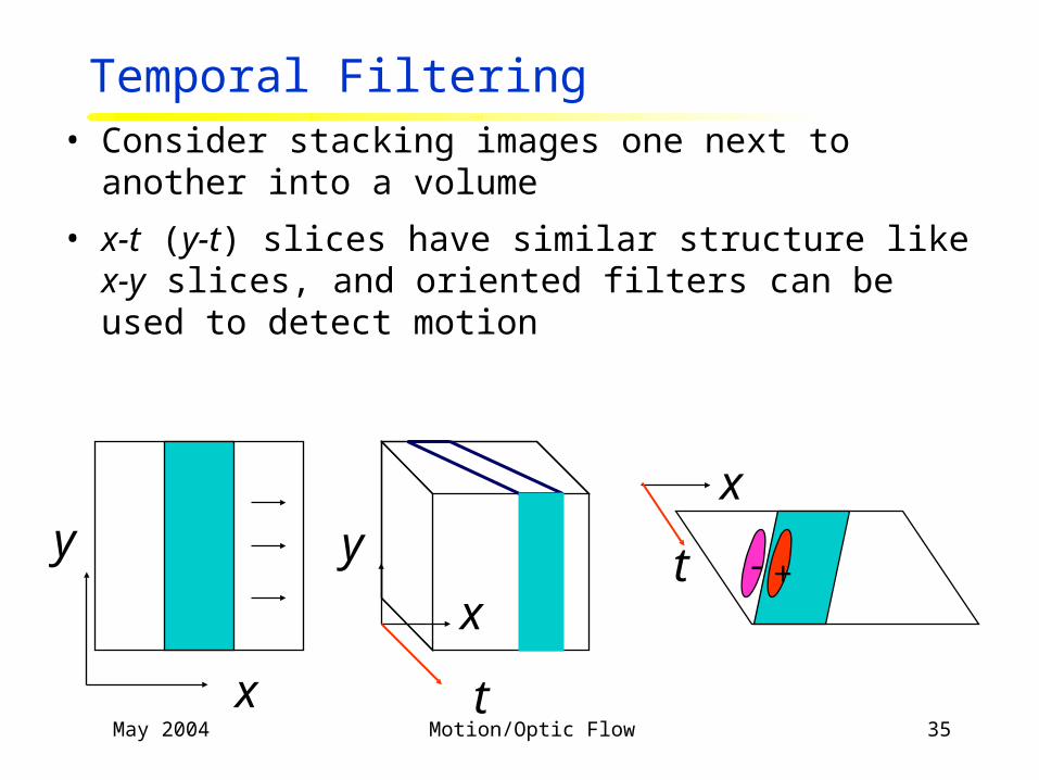
Temporal Filtering• Consider stacking images one next to another into a volume

• x-t (y-t) slices have similar structure like x-y slices, and oriented filters can be used to detect motion

x

x

y y

t

x

t +-


Approach

• The response of a detection cell must be both temporal and spatial varying

• A popular function for that is the Gabor function– Gaussian modulated sin curve

)222sin(2

1 )222

(2

2

2

2

2

2

twywxwe tyx

xxx

tyx

tyx πππσσσπ

σσσ ++++−


Why?

• The filter is separable, meaning that filter shape in different dimension can be designed separately and then combined

• By Fourier transform theory – The sigma controls the spread in a dimension

– The omega controls the center frequency A band pass filter of different orientation and frequency selectivity


Beyond OF: Structure from Motion

• Possible to recover camera motion and scene structure from a video sequence.

• Information about the movement of brightness patterns at only a few points can be used to determine the motion of the camera.– In general, seven points are sufficient to determine the motion

uniquely.

• In the case of pure translation, the optical flow vectors all pass through a point when extended.

• This point where the optical flow is zero is called the focus of expansion.– It is the image of the ray along which the camera moves.


MF & OF Summary

• Motion field

• Optical flow

• MF not the same as OF

• Optical flow constraint equation

• Aperture problem


Next Class and Next Week

• Thursday: Application to Image databases– MPEG-7 standard

– A presentation by Till Quack on a web image search engine

• FRIDAY discussion: review optical flow. – Note that this will be the last discussion session. Monday is a

holiday, so *all* students are encouraged to attend the Friday meeting.

• Next Tuesday: Project review and discussions

• Next Thursday: Course review and conclusions.

may 2004motion/optic flow1 motion field and optical flow ack, for the slides: professor yuan-fang...

Documents