May 21, 2016 Evolution of Igpet, a Graphics and Modeling Program for Igneous Petrology Michael J. Carr Department of Geological Sciences, Rutgers University, 610 Taylor Road, Piscataway, New Jersey 08854-8066, USA (carr@rutgers.edu) Esteban Gazel Deparment of Geosciences, Virginia Tech, Derring Hall (0420) Blacksburg, Virginia 24061, USA (egazel@vt.edu) Abstract The Igpet program evolved to satisfy three basic requirements for improving productivity in the fields of petrology and geochemistry. The initial goal was to provide an intuitive interface that allowed users to rapidly display data to determine if a known pattern of magmatic evolution was present. As scientific communication became fully digital, the next goal was creating publication quality figures that could be included into articles with little or no editing. Finally, powerful modeling became a requirement because quantitative evaluation of petrologic processes is a normal component of publications. Igpet allows testing of forward models of magmatic evolution using equations for trace elements and radiogenic isotopes subjected to melting, crystallization, assimilation and mixing. Igpet includes inverse modeling using the rare earth elements (REEs) and the tracing of magma evolution via pseudoquaternary projections of phase diagrams. Programming to achieve these goals extended in three directions. Data handing evolved toward placing the information for complex diagrams entirely in easily edited text files. The handling of petrologic and geochemical data evolved to use text files, to storing data as string variables and to making few or no changes to the original data files. The user interface stressed rapid display of plots with a minimum of user input, such as just a couple of mouse clicks. An initial preference for multiple small data files was replaced by controls that allowed large data files (e.g. several volcanoes) to be plotted as one or to be rapidly sorted to zoom into particular subsets. This allows comparisons among subsets (e.g. volcanoes) without the need to read a new data file. Finally, Igpet had to incorporate numerous algorithms to model igneous processes and many of these are specified here in the Xojo language, a modern language evolved from BASIC. Introduction Igpet is an interactive program for displaying and modeling geochemical data pertinent to Igneous Petrology. It started as a utility to facilitate data entry and then make accurate plots which could be given to a draftsperson for publication quality figures. The first highly useful version of Igpet was written on an IBM PC in 1984 to take advantage of having sole possession of a computer with is green and black screen. This allowed what has always been the greatest strength of this software: immediate feedback with a flexible interface to rapidly create diagrams based on any geochemical parameter or combination

2

of parameters that could be plotted in XY, Triangular or Spider plots. All of the development of Igpet occurred when a need was recognized for more user control, new diagrams or more flexible and comprehensive modeling. Because Igpet has been written and rewritten over more than 30 years and has transitioned from BASIC to Fortran to Basica (for IBM-PC), to GWBasic to Microsoft Basic to several versions of Visual Basic up to Visual Basic 6 (VB6) to REALBasic and now Xojo, it is not a well-written program. Furthermore, many dead ends were jettisoned, including CalComp plotter code, HPGL code for early HP laser printers and plotters and an entire version of Igpet written in Microsoft Basic for the Mac. Evolution is a valid metaphor for describing how Igpet attained its current form. Although many obsolete technologies have been completely excised, there are some early functions of Igpet that remain as vestigial trappings that are unlikely to be used but do not appear to be causing harm. The primary example of this is a routine in the file operations menu of the Windows version that helps a user type data in by setting the order of elements to be the same as the order on the printed page. Excel or any other spreadsheet makes this capability redundant. The main programmatic thrust driving Igpet’s evolution is the need for independent modules or objects as opposed to Igpet’s initial design which was to start with the first card in a deck and proceed to the end and do specified jobs along the way. Currently, Igpet has way too many global variables and too little control over adverse outcomes when a global variable is changed and then referenced again in an unanticipated way. With every iteration, Igpet improves or becomes more object oriented but from a programming perspective it is still a primitive construct. Nevertheless, Igpet is useful and does its main job well. The experience gained from decades of interaction with users and from repeatedly porting from one operating system to the next led to three goals that crystallized during Igpet’s evolution. First, a primary requirement, excellent graphics output that can be included with little or no editing into publications. In Windows this is accomplished using the 32 bit Applications Programming Interface (API) and Graphics Device Interface (GDI) functions to create vector graphics that can be sent to the clipboard, from which they can be imported into programs such as Word, Powerpoint and Adobe Illustrator (AI). The Windows version uses VB6, which is considerably out of date. In Windows there is one set of commands for all output but very different input into those commands depending on whether the screen or another output device is the target. The Mac OS X version uses the Xojo programming language, which is also 32 bit but is modern and frequently updated. In this case, there are separate routines for low quality screen output and high quality PDF output. The DynaPDF module from MonkeyBread Software provides the commands that make the PDF graphics. Because the goal of high quality vector graphics output involves three independent programming languages or modules and because it is more about programming details than about developing a useful system to facilitate the interpretation of igneous rocks, it will not be considered further.

3

The second goal is an interface that improves in the direction of more intuitive use. This is a process not a final result. User suggestions and frustrations are the primary source of interface improvements followed by pruning of redundant steps and deactivation of menu options and command buttons when context makes them irrelevant (or dangerous). Accidents also helped, as unplanned results from using incompletely understood functions have sometimes led to serendipitous utility. An intuitive user interface is an important research goal in Computer Science and the results in Igpet are perhaps useful only as an example of a trial and error process. Two aspects of the user interface will be emphasized below, data handling and controls. The third goal is powerful modeling. The major processes of geochemical evolution in igneous rocks can be traced via forward modeling using equations for trace elements and radiogenic isotopes subjected to melting, crystallization, assimilation and mixing. Igpet’s modeling capability has improved over time and the current most powerful modeling begins with a spider-diagram comprised of a large number of elements with different behaviors. Commonly used spider-diagrams typically include large ionic radius lithophile (LIL), high field strength (HFS) and rare earth elements (REE). The power in the modeling arises from simultaneously subjecting all the elements in a spider plot to the same modeling steps. For example, three source components are mixed and the mixture then subjected to 1%, 5% and 10% partial melting using the aggregated fractional melting model with a specified mantle mineral mode, a specified melt mode and a set of appropriate partition coefficients. All the calculated models remain in memory for display in spider-diagrams or in XY plots of elements or element ratios. The models can be preserved for later use by saving the data to a new file. The modeling tools or algorithms in Igpet are described below along with some case studies demonstrating how the modeling can be applied.. User interface: Data handling Geochemical data and metadata The initial versions of Igpet had all numeric input and specified a particular order for the 11 major oxides in igneous rocks. The current version is nearly the opposite with all input read as string variables and a flexible order of elements and other data. The principle here is to do as little as possible to the user’s original data. Most individual data sets are now in spreadsheets that contain numeric data and alphanumeric descriptions or metadata. Many instruments provide output as Excel spreadsheets, so this is, in effect, the native format of geochemical data. Raw or pristine data should not be disturbed and, of course, should be robustly backed up. Because spreadsheets can write and read tab delimited text files and because these files are easy to read and write using programming languages, the tab delimited txt file is the basis for Igpet input. For data files, Igpet requires up to four special columns. The first is “samp” because there are many instances in Igpet where individual samples have to be selected by name. The other three columns are “Jcode, Kcode, Lcode” all of which consist of integers between 0 and 36. These code for the 37 symbols available in Igpet. Having three separate symbol codes allows one to subdivide data sets in three separate dimensions. This is too much

4

flexibility for a small data set but for the data file that coevolved with Igpet, RU_CAGeochem (Carr et al., 2014), it is necessary because there are 15 geographic-geochemical groupings (Kcodes), 40 distinct volcanic centers and multiple units within different volcanic centers (Lcodes). Because Kcode is the default code to associate with a symbol, Igpet works better if a column called Kcode is added to a data file. The minimum modifications of a spreadsheet that Igpet requires are: first, changing the column header for the name column to include the string “samp” where case is not important. Second, the sample name column should be the first one to include “samp” in the column header, all later occurrences of “samp” among the column headers will be ignored. Third, it is best to add a column called Kcode to specify symbols using integers. Fourth, if there is more than one column for an element (xrf value, icp value etc), the non-preferred data columns should have an x added to the front of the column name. All data upgrade and maintenance should be made to the spreadsheet file (typically an xls or xlsx file). This allows the tab delimited txt files, used by Igpet, to have secondary importance so that they can be deleted without risk. The data Igpet reads are held in a matrix whose size can be set at runtime. The default setting at present happens to be 13,000 rows or samples by 250 columns of oxides, elements, locations, descriptors etc. This can be reset using the Preferences tab on the main menu. Because the data can include descriptors such as “lava” or “tephra” the logical choice is the make the data matrix a string variable. Igpet uses u(row, column) for the main matrix because years ago all Igpet data was single precision and m() was by default an integer variable in FORTRAN. Numeric values for igneous parameters like SiO2 are obtained, as needed, by a subroutine that uses international awareness to convert values like 52.65 or 52,65 to a single precision numeric value. Keeping the oxide, element and other numeric values in string form also prevents conversion errors if the user decides to save the data file to a new name because of new models that were created. Although the data conversion from string to numeric value takes some amount of time, it is not perceptible on modern computers, even when plotting several hundred samples. The order of igneous data is not universal or systematic but there are many particular calculations that require specific oxides or elements, therefore Igpet does extensive searching and aliasing. Immediately after reading a data file, Igpet locates the column positions of the major oxides and stores these in a vector. For isotopic calculations the concentrations of elements like Sr, Nd, Pb etc are needed so the variables iSr, iNd etc store the positions of these elements. Similarly, NiO and Cr2O3 are needed in several calculations so the positions of Ni and Cr are stored in case the oxide values are not included. Finally, the names of each column are searched and compared with a vector of preferred column names (variable names) that include keys to upper and lower case. Thus SIO2 or sio2 in a data file becomes SiO[2] in the vector that Igpet uses for variable names. The [] brackets cause a subscript and {} cause a superscript. The cleaning up of the column names is not perfect: for example, “sr iso” does not get converted to {87}Sr/{86}Sr. A significant problem here is the addition of (WT%) or (PPM) to the column names of oxides and elements. Igpet attempts to remove these qualifiers but is

5

not smart enough to eliminate all variants. If an element name includes “ppb” this modifier is not removed. The largest reported problem with column names is the replication of oxide names or ppm names. Some data sets include Fe2O3, FeO, FeOt or FeO*. Of all the variants of Fe, Igpet would prefer just the actual values of Fe2O3 and FeO. If one Fe oxide is not reported, let it be a blank on the spreadsheet. Igpet has routines to calculate FeO* and to apportion Fe between the Fe++ and Fe+++ oxidation states. Putting in both Fe2O3 and 0.8998*Fe2O3 as the value of FeO results in a doubling of the molecules of Fe and causes a mess in several dimensions. Another reported problem is the replication of trace element values using different techniques, e.g. Sr XRF, Sr ICP etc. For spider-diagrams and calculations involving isotopes it is best to pick a preferred value and call that Sr with no extension. The alternate values are most safely kept with an “x” added to the front, e.g. xSr XRF, so that Igpet unambiguously finds the correct value. Finally, some files get huge by accident and Igpet cannot read them, even when the actual dimensions of the data are modest. The cause is some mistake in using the spreadsheet program that causes thousands of blank lines. This problem can be fixed in the spreadsheet program by highlighting the actual data and copying it into a new sheet. File Operations, a submenu of File, is a very old part of Igpet that retains three useful functions. Modify (Windows) or View (Mac), is a button that allows you to view the contents of the data matrix, u(row, column). The Windows version allows editing here but editing in a spreadsheet is a much better approach. The Mac version is limited to displaying 64 columns. When something is wrong with a plot or calculation, the first step toward resolving the problem is to examine the data matrix and compare that to the original values in the spreadsheet. The Add a file button is very valuable. You can access this button only if you already have a data file in memory. When adding a file, the new data are entered in the same order as the original file. It is often useful to merge data sets and rarely do they have the same order. The caution required here is that data columns in the second file that are not in the first file will be lost. Furthermore, the column headers in the second file should be edited if necessary to be sure that they will be recognized. A trial and error process can be used as long as the output file name is always different from either of the two input files! After the files have been merged, a new file should be created with the Save button. Similarly, if a modeling session has been successful and the results are worth saving, use the Save button to make a new file. Migration of control information to files and folders The Igpet folder is normally placed in the Applications folder (Mac) or in Program Files (x86) for Windows. The folder structure of Igpet consists of six subfolders that contain about 80 files (Figure 1). Most of the files are tab delimited txt files that can be edited and thus controlled by the user.

6

Data for igneous petrology include many fixed or nearly fixed quantities, such as molecular weights of the oxides, the cations per molecule, the factors for converting oxides to ppm, the preferred oxide names and related trace element names, etc. Rather than building these values into the code, it is valuable to have them accessible as a resource for quick reference. They are stored in the folder called Controls in a file called igpetdata.txt. Also included in this file are the parameters needed to calculate the density of a magma (Bottinga and Weill, 1970) and the parameters for adjusting the Fe++/Fe+++ ratio in magmas at one atmosphere pressure, given a specified temperature and fO2 following Beattie (1993) and Kress and Carmichael (1991). This file also contains the preferred names of isotope ratios and trace elements, so that, for example, RB in a column header gets stored in Igpet as Rb. Igprefini.txt stores the results of preferences that are selected in the Preferences tab of the main menu. This file should be modified during the first run of Igpet to select screen size, path to data files, default matrix size and several other variables. Less likely to be edited is Page.txt that contains the dimensions of 16 possible plotting regions on an 8 by 10.25 inch page. There are several files that define the 37 symbols used by Igpet. Several users have created their own symbol files based on the default version but most users stay with default.sym.txt. A file called Extra.txt holds several commonly used oxide and element combinations that can be added to the data in memory (Mg# is the calculation most often used). A frequently used file, called Spider.txt, holds all the spider-diagram definitions. There is even a file, PercentFs.txt, that holds suggested F values for different melting and crystallization models in the spider modeling window. Because of the numerous editable files in the Igpet system, very little remains that is hard coded into the software. Earlier versions of Igpet were mostly hard coded but now the largest part of Igpet that remains hard coded is one of the oldest calculations in igneous petrology. This is the Cross, Iddings, Pirsson and Washington (1902) method of estimating the mineral percentages that should be found in a fully crystallized magma (CIPW Norm). Data handing and file formatting is discussed in the manual that accompanies the Igpet program, but experience shows that the manual is either poorly written, little used or both. User complaints were reduced as the data file structure was made as flexible as possible. Perhaps the least appreciated aspect of data handing is Igpet’s ability to substitute preferred variable names for the users column names, allowing better quality labeling without any user effort. Finally, placing as much control as possible in easily editable txt files allows customization even if few users need it. User interface: controls Rapid feedback encourages exploration, therefore many aspects of the Igpet interface were designed to get the user’s data displayed on the screen as easily as possible. Opening a file can be a tedious slog through multiple layers of folders so, as is common with most programs now, the File menu includes a list of the last 5 files opened allowing

7

immediate return. Furthermore, the Preferences menu allows selection of a folder where Igpet will expect to find data files. As Igpet opens, the only active control is the File menu. As soon as the user selects a file, many other menu items and control buttons activate. The Plot menu is likely the user’s next choice and XY plots are the most common type in igneous petrology. Assuming this path, Igpet presents a window of buttons from which to select an X variable and then a Y variable, and so only two clicks are needed. As soon as Y is selected the plot is made. The scaling of the plot is automatic because Igpet was designed for rapid turnover of plots, for quick views of “what if” scenarios. The automatic scaling is a hazard if a user’s samples are all very similar. In that case a small range in X or Y will fill the screen and primarily reveal the random noise inherent in geochemical analysis. This is a significant weakness but one that is overcome with experience. The scaling algorithm is: Determine maximum and minimum factor=10^INT(Log10(max-min)) Begin=factor*INT(min/factor) End=factor*INT(1+max/factor) Similar logic sets the default tick spacing and label steps. All of these graphic elements can be modified by clicking the Axis control button but this can wait until after a useful plot is uncovered. A new X or Y variable can be selected with two mouse clicks. Other single click options include reversing the X and Y axes and flipping the order in which the data are plotted, which is useful where there are 50 or more overlapping data points and the early ones are buried. The main window for the Mac and Windows versions diverged during a period when the software used for the Mac version did not provide a path to excellent graphics output. The Windows version was given a cleaner appearance by moving 12 functions to an Edit menu, leaving just a double row of buttons on the top of the window. The Mac version, an older design, still has all image and modeling controls in 26 buttons on the top and left side of the main window. As a result, the Mac version is more responsive and slightly simpler to use. Users prefer single click access to functions rather than the two clicks needed for menu items. The Plot menu allows the choice of XY, TRI, Histogram, Spider, CMAS, Diagram and Mineral. The first three choices open the Variable window where X, Y and Z are selected, using either a button, a series of button functions (+, *, /, Log etc) or a text box for writing an equation. Igpet has an equation parser that recursively examines equations expressed as text strings and calculates the value of the equation. The other Plot options call pre-designed diagrams that are selected in a combination of file menus and list boxes. The choice of a plot type deactivates or changes the purpose of several of the controls depending on the nature of the plot to be made. This restriction of options is necessary to prevent unanticipated outcomes and also for steering users to the useful paths. Getting these settings correct is important because if a button is present it will be pushed, if only for curiosity. Managing the interface is accomplished in two subroutines, one that turns

8

everything off and a more complex one that turns on and re-labels the buttons and menu items that are needed for the specific Plot option chosen. Igpet provides multiple methods for identifying each sample. For a small data set a Name button writes the sample name adjacent to each sample. For large datasets an Identify button can be turned on or off. When on, a click on the diagram will cause the nearest sample to be highlighted and named. If one seeks a particular sample, there is a Pick button that brings up a list box holding all the sample names to pick from. Assuming the file uses different symbols for subsets of the data, one can use the Symbols window to choose which symbols to plot. One can also choose an alternate integer vector for keying the symbols. The default is Kcode but Jcode and Lcode are available. Once the appropriate symbol key is selected, one can pick and choose which symbols to plot or hide, allowing rapid identification and comparison of different subsets. The strong emphasis on identifying particular samples had two origins: the first was a preference for subdividing data into meaningful groups rather than assuming the data are from a single magmatic unit. The three different symbol codes allow coarse, medium and fine-grained subdivisions of the data and near immediate switching between these options. This is useful because what might seem like a clear geochemical discrimination of groups in one plane may fail completely when looking at the data in a different dimension. The second motivation for identifying particular samples is the need to find end-members for geochemical modeling. Exploring an igneous data set is now a large task. At the onset of the Igpet program, geochemical data consisted of 11 major elements and about 6 trace elements. Now about 35 trace elements and six radiogenic isotope ratios are commonly reported along with the major elements. A vast number of plot combinations are possible but there is substantial co-linearity among the elements so the number of useful elements can be reduced. For example, La, Eu, Sm and Yb or Lu can represent most of the variation of the 15 rare earth elements. Taking just trace elements well determined by ICPMS and removing most of the REEs results in 15 elements; Cs, K, Rb, U, Th, Nb, Ta, La, Gd, Yb, Zr, Hf, Pb, Sr, Ti. This list can be further trimmed of Hf and Ta, which behave like Zr and Nb, but, even so, for XY plots there are 13 elements from which to pick 2 or 78 combinations. It is common to plot trace element ratios, so there are 13 elements from which to pick 4 or 715 ratio-ratio plots, most of which will never be used. The real complexity is not as bad as the large number of combinations suggest. One approach to regain manageable simplicity is emulation of previous work, which is not particularly creative but is a necessary starting point. Another approach is to identify the sources that contributed to the magma and discover those elements that differ the most between the sources. Such elements will provide the clearest window into the melting and assimilation processes that create complex evolutionary patterns. The complexity caused by the major expansion of analytical capability was a major driving force in developing fast and flexible plotting methods. If an entire region or magma type is the subject of a research project, the data file can be very large. An extreme example is the database of mid-ocean ridge glasses (the Volcanic

9

Glass File, maintained by the Department of Mineral Sciences at the Smithsonian Institution: http://mineralsciences.si.edu/research/glass/vg.htm, Melson et al., 2002), which now has more than 12,000 entries. Early versions of Igpet had size limitations that prevented reading an older version of this database, when it had fewer than 2,000 entries. For some purposes, all the data need to be plotted, but for other cases, such as a particular rift segment, only a small subset of the data is required. Initially, Igpet was designed for many small data files, one for each volcano or rift segment or other type of focus region. Experience with RU_CAGeochem established that it is much easier to maintain and upgrade a single large data file rather than multiple small ones. Therefore, Igpet needed a tool that emulated the sorts of questions and limits that are found in querying databases. A SubSelect window was developed that allowed multiple inclusions, exclusions and numerical ranges. The first window in SubSelect is a listbox that contains all the variable names (column headers). Select a variable with a click and the next window, also a listbox, fills with all the sample names and the values for the selected variable. If the variable is a string, like volcano name, then the Include or Exclude listbox can be activated and particular volcanoes either selected or excluded. If the variable is a number, like SiO2, the maximum and minimum values are entered and then saved to the Limits listbox. SubSelect is a powerful tool that facilitates comparisons among related groups, such as the 40 different volcanic centers in RU_CAGeochem. An intricate plot can be devised and then examined, volcano by volcano, just by changing the volcano name in the Include listbox. Modern laptops don’t seem to be limited by memory at least for the sizes of reasonable geochemical data sets, so now a single file with all one’s data can be used. This approach is much easier to maintain and speeds up many types of comparisons among different data dimensions. Some versions of Igpet had the ability to directly read spreadsheet files (e.g. .xls files). The software tools to enable this added significantly to the size of the compiled program and greatly slowed down the file read process. The direct use of a spreadsheet file also created risk because it allowed users to not bother to make a back up. The current Igpet file reading system nudges users to maintain their data in a spreadsheet file and make copies into a tab delimited txt file for use in Igpet. This creates at least one layer of backup. Igpet has never been able to interact with a database, even though almost all the programming languages that Igpet has been written in have substantial database capabilities. This lacuna is primarily a flaw arising from the preferences or prejudices of the creator of Igpet. For many years, observation of Igpet users revealed high levels of skill in using spreadsheets and practically no experience with databases. However, the availability of large international geochemical databases is removing that weakness. An excellent international database of volcanic rock geochemistry, GEOROC (Geochemistry of Rocks of the Oceans and Continents at Max Planck Institute for Chemistry in Mainz), provides output as comma separated txt files (.csv files) and provides instructions for reading them in Excel. Igpet uses tab delimited txt files (.txt) that are equally easy to read in Excel and so, the native file format of Igpet seems acceptable. Recognizing the widespread use of GEOROC and consistent with the goal of improving the user interface Igpet now reads the .csv files output by GEOROC.

10

Modeling Algorithms Merely plotting igneous data is not sufficient. Simple and sophisticated forward modeling tools allow hypothesis testing but require some sophisticated understanding of the models of magmatic evolution from melting to crystallization. Fortunately, Albarede (1995) comprehensively explains and derives a great many models of magma evolution. Converting the equations in Albarede (1995) to algorithms allowed sophisticated forward modeling in Igpet. The models simultaneously calculate the concentrations of all the trace elements in the multi-element plot (Spider diagram) selected. An earlier set of modeling tools was written for XY plots using DePaolo (1981). The primary algorithm for geochemical mixing was taken from Langmuir et al. (1977). The Igpet manual does not attempt to replicate the assumptions, formalities or insights from these important references but instead encourages users to go to these sources. The algorithms derived from the references above are the most important part of Igpet and will be described below after treating several other calculations that are peculiar to igneous petrology. The norm (Cross et al., 1902) provides Petrology teachers with a means for testing the rules following and arithmetic skills of undergraduates. It is fundamentally out of date for research but has pedagogical value because it provides the logic for defining three types of basalts, those with quartz, those with hypersthene but no quartz, and those with nepheline. The latter type develops along a substantially different evolutionary path and creates a spectrum of alkaline lavas. During the 1970’s several computer programs were available for calculating the CIPW norm. The four that were tested for the earliest version of Igpet all produced different answers. A search for resolution led to Johannsen (1931), a comprehensive treatise on descriptive petrology. The CIPW norms in this text covered a wide range of igneous rocks, testing the limits of the full CIPW calculation. However, most of the worked examples were flawed and Johannsen had located and carefully described the error. Thus, it did not seem necessary to find a perfect CIPW calculation. The most comprehensive norm available, a FORTRAN program (Van Niekerk and Von Backström, 1966) was translated into BASIC and tested against the original using normal to extreme igneous rock compositions, including several from Johannsen (1931). The test data file, CIPWtest.txt, remains in Igpet. The CIPW norm remains quite useful in igneous rock nomenclature as shown in Figure 2. Analyses of rocks sum to 100% but most of the mass is in SiO2. Whether analytical error is random or systematic, most of the error will be in SiO2. It is common to plot SiO2 as the x-variable and compare variations in other oxides or elements to it (Harker plots). Because most error is in silica, some noise reduction occurs if analyses are recalculated to 100% on a water free basis with all Fe expressed as FeO. Furthermore, many discrimination plots require this. Igpet turns this normalization on and off without affecting the original data, which are stored as string values and never altered. To do so, after a file is read, a total of the oxides (without water and with all Fe as FeO) is calculated for each sample (row in the matrix) and stored in a vector. If the Norm to 100% option is clicked, a list box of all the variables is presented. The major oxides have a * added to the left of their descriptor (e.g. *MgO) indicating this parameter will be

11

multiplied by 100/total. Trace elements, included in the list of preferred names in igpetdata.txt file, also get marked but any preferred name including / is not marked. The user can then adjust the list that will be normalized by double clicking an element to add or remove the *. Normalization to 100% is automatically done on several predesigned diagrams where the authors of the diagram made that condition part of the definition of the diagram. Users have complained about this automatic normalization but, in this case, it is best to make the diagram accurately rather provide flexibility. A file called Extra.txt includes the equations of several commonly used combinations of oxides and elements. Clicking the Add Extra Parameters menuitem adds 16 new parameters. The first four, density, Ce*, Eu* and Nb*, are complicated and hard coded into the subroutine. Density is estimated dry at 1 atmosphere following Bottinga and Weill (1970). Eu* is the value estimated from adjacent rare earth elements, Sm and Gd. xsm = CSingle(u(i, ksm)) / 0.153 ‘ ksm is the position of Sm ‘ CSingle converts string to number ‘ 0.153 is the chondritic value of Sm xgd = CSingle(u(i, kgd)) / 0.2055 xeu = CSingle(u(i, keu)) / 0.058 cx = xsm * xgd ‘ a test-because Log (0) is undefined If cx > 0 Then ‘ values exist for Gd and Sm, proceed ax = 0.5 * (Log(xsm) / 2.302585 + Log(xgd) / 2.302585) ‘ Log is natural log ax = 0.058 * Exp(2.302585 * ax) ‘ 0.058 is the Chondritic value of Eu u(i, kEu*) = str(ax) ‘New parameter Eu* stored as a string End if Similar logic applies to Ce* and Nb* but Ce* is referenced to La and Pr and Nb* to La and Nd. The other parameters in Extra.txt. are calculated with the equation parser that uses recursion to evaluate equations and calculate a new parameter. The entries in Extra.txt include the parameter name, a condition, and the equation; some examples are given below. The condition ‘zerosin’ means that it is acceptable if one of the components of the equation is zero. In many instances, either Fe2O3 or FeO is not reported but that does not cause an invalid calculation of FeO* or Mg#, thus ‘zerosin.’ The eNd calculation assumes a zero age sample. The use of quotations tells the recursion routine to ignore the / and * inside the quotes and treat the entire string as a variable name. FeO* zerosin FeO+Fe2O3*.8998 Mg# zerosin MgO*2.481/(MgO*.0248+FeO*.013918+Fe2O3*.012523) Ba/La nozeros Ba/La eNd nozeros "{143}Nd/{144}Nd"*19505.344464383241-10000 Eu/Eu* nozeros Eu/"Eu*"

12

Inexplicably, the calculation of Mg# has commonly been perturbed as Igpet has evolved. It has been a recurrent bug but now that it is in a text file rather than in code, it may remain stable. The partitioning of Fe into FeO and Fe2O3 is important but the chemical analysis can be difficult and lavas are subject to oxidation during cooling and subsequent weathering. Therefore, many whole rock analyses no longer include separate measurements of these two oxides. Data obtained by XRF are usually presented as Fe2O3, but other analytical techniques commonly report FeO because in most rocks the majority of the Fe is in the Fe++ state. Two methods are included in Igpet to set the whole rock Fe++/Fe+++ ratio. In the CIPW norm, Fe can be partitioned according to the rule in the Irvine and Baragar (1971) rock classification system where a provisional Fe2O3 is set to 1.5+TiO2. If the analysis value is less than this, no change is made, otherwise this is the new value of Fe2O3 and the remaining Fe is put into FeO. For the creation of pseudoquaterary phase diagrams (CMAS projections) FeO and Fe2O3 can be reset along a specified oxygen buffer following the algorithms of Beattie (1993) for temperature and Kress and Carmichael (1991) for the iron partitioning at specified T and fO2. The oxygen buffers used are: NNO fo2 = (-478967 + 248.514 * T - 9.7961 * T * Log(T)) / (8.31441 * T * 2.302585) QFM fo2 = (-587474 + 1584.427 * T - 203.3164 * T * Log(T) + 0.09271 * T*T)/ (8.31441 * T * 2.302585) IW fo2 = (-550915 + 269.106 * T - 16.9484 * T * Log(T)) / (8.31441 * T * 2.302585) XY modeling In X-Y plots, the simplest type of modeling is least squares regression. For example, magma mixing should create a linear array in element-element plots. Igpet uses the algorithms in Davis (1973) for linear regression and the Pearson correlation coefficient. After transformation of variables, the same logic allows polynomial regression and hyperbolic regression. Spearman’s rank correlation coefficient was calculated using equations from Swan and Sandilands (1995). Statistical parameters were checked against the data sets and results in Swan and Sandilands (1995). The earliest magma evolution models in Igpet use the equations of Langmuir et al. (1977) for mixing and DePaolo (1981) for AFC (assimilation-fractional crystallization) processes. The limitations of modeling in an Igpet XY plot are that only 2 to 4 elements are involved and the results are only displayed as curves on the XY diagram and are not saved in the main matrix for further use. Furthermore, the AFC calculations require a bulk partition coefficient, D, which is entered in a text box rather than calculated from a mantle mode and appropriate partition coefficients. Because of the relative simplicity of

13

dealing with just two elements or two element ratios and the immediate graphical feedback showing the results of changing assumptions about D and the range of F (percent fluid) values, the XY Mix and Model tools are particularly valuable for teaching. Because of the nature of AFC equations, mixing, fractional crystallization and assimilation coupled with fractional crystallization use the same logic. The equations of DePaolo (1981) used in Igpet for trace elements and radiogenic isotopes are 3, 6a, and 6b. Equation 3: condition: assimilation rate equals crystallization rate (r=1) z a temporary value c concentration in melt co initial concentration of element in magma ca concentration of element in assimilant D bulk distribution coefficient f mass of assimilant/mass of magma or Ma/Mm (f varies from 1 to 0.001) z= Exp(-D * f) Exp is the exponential function in Xojo c = co * z+ (1 - z) * ca / D equation for zone refining Equation 6a: condition: r not equal to 1 r rate of assimilation/rate of crystallization f mass of magma/initial mass of magma or Mm/Mmo

if r<1 then f varies from 1 to 0.1) if r>1 then f varies from 1 to 5 or more

z=(r+D-1)/(r-1) c = co * pow(f ,-z) + ca * r * (1 - pow(f, -z)) / (r-1) equation for AFC

where pow is the Xojo function for f-z

This is the general algorithm for AFC. If there is no assimilation, r=0 and ca=0 then the equation simplifies to the well known equation for fractional crystallization. In the special case where r+D-1=0 then z is 0 and equation 6b is needed: c = co + r * ca * Log(f) / (r - 1) The radiogenic isotopes can also be calculated with equation 15b. Calculate SrIsoRatio given the following values: F(j) = ‘ Fvalue for step j afc0 = ‘Sr content of original/initial magma afcVal) = ‘Sr content of assimilant or 2nd magma for Mixing afc0I = ‘isotopic ratio initial magma afcAI = ‘isotopic ratio assimilant SrIsoRatio = afc0I + (afcAI - afc0I) * (1 - (afc0 / afcVal)/F(j)) '15b

14

The equilibrium melting and crystallization processes are also included in the XY model tool. c = co / (f + d - f * d) equilibrium melting and, for variety, the same equation in different form c = co / f + d * (1 - f) equilibrium crystallization In the XY models, the algorithms shown above sequentially calculate concentrations for up to 4 elements or pseudo-elements, depending on the X and Y variables selected. An appropriate range of f values is suggested depending on the model selected and other conditions such as the value of r. The user adjusts the suggested start, stop and step of f. These values define an f loop that brackets the element concentration loop. Igpet calculates the 4 concentrations at the specified f values and at five intermediate f values as well, in order to provide a reasonably smooth curve. The model is drawn onto the existing XY diagram. Each model is added to the diagram, so that the effects of changing co, ca, r, D etc can be observed. To remove all the models, one clicks the new X or new Y button and remakes the plot with just the data. Mixing of sources or magmas generally results in a hyperbola that describes the intermediate compositions (Langmuir et al., 1977) but in the case of Pb isotope plots the hyperbola is reduced to a line because the three commonly used Pb isotope ratios all have the same denominator, 204Pb. The hyperbola constants can be determined from two points or calculated from all the points using least squares. Because a hyperbola has two branches least squares may fit a data set with moderate scatter using both branches, which is a meaningless solution. Determining mixes using two points is the more practical approach. If the data set is fit by least squares, the argument that mixing has occurred becomes more convincing. Figure 4 is an example of a ratio/ratio plot in which the data define a robust hyperbola using the least squares method. Radiogenic isotopic ratios for Sr, Nd, Pb and Hf are reformed into two pseudo elements in the same manner as described above for Sr. Therefore, mixing calculations for these ratios cannot be done unless the elemental concentration is also reported. The four constants in the hyperbola equation can be determined from two well-separated points. The equation is: Ax + Bxy + Cy + D = 0 Consider a ratio/ratio plot with points 1 and 2. Let the ratio for X be p/q and the ratio for Y be r/s. The constants of the hyperbola equation are: A = q1 * r2 - q2 * r1 B = q2 * s1 - q1 * s2 C = s2 * p1 - s1 * p2

15

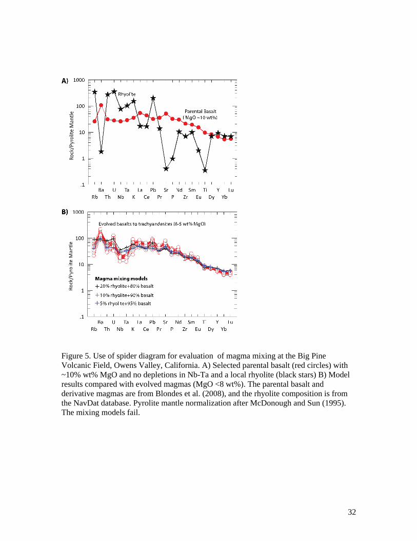
D = p2 * r1 - p1 * r2 To determine these constants, the user identifies two appropriate end members and then selects them from a listbox. For elements, Igpet keeps track of the column positions of the elements in the plot, usually there are four, p, q, r and s. The end member selections provide the row positions for points 1 and 2 and the hyperbola constants are readily calculated. The X difference between points 1 and 2 is divided into 100 increments to generate a smooth curve. The Y values are obtained by solving the hyperbola equation for Y. yi = -(D + A * xi) / (C + B * xi) the xi, yi pairs are temporarily stored for plotting. The user can modify the choice of end members and generate a family of mixing hyperbolas. As is the case with the AFC models, the curves are saved as graphics but not stored in memory. The ease of making mixing hyperbolae is much greater than their significance and so users of Igpet likely overuse this tool. Solid sources may well mix but likely on fairly long time scales. It is more likely that fluids mix and melts and hydrous fluids mix more readily than magmas with crystals which are likely to be much more viscous. In both mafic lavas and silicic tephras, there are many indications of mixing so this is a common process although it is likely coupled with fractional crystallization in the majority of cases. Multi-element mixing Multi-element mixing and modeling is more realistic than the XY models described above. A spider-diagram is a convenient display of 15 to 30 minor and trace elements. In a Spider plot, the Mix button brings up a window with text boxes that allows calculation of complex mixes. Up to 5 components can be mixed using integer weights, decimal fractions or %s. Thus, 3,1 and .75, .25 and 75, 25 produce the same result when mixing two components. Five samples can be averaged giving each a weight of 1. A specific mantle can be calculated by adding end-member mantle components, e.g. 95 DMM and 5 HIMU. The isotope ratios calculated by the Spider-Mix button use the logic described above for the XY models. The isotope ratio and concentration are used to make pseudo-element values, e.g. 87Srppm and 86Srppm. After the mix calculation the isotope ratio of the mix is calculated from the pseudo-elements. Epsilon values cannot be mixed in this routine. Case study of Magma Mixing As an example of multi-element mixing we used the Spider plot option to investigate the source of Nb and Ta anomalies in evolved basalts to basaltic tracy-andesites with MgO<8wt% at the Big Pine Volcanic Field, Owens Valley, California (Blondes et al. 2008; Gazel et al, 2011). Our first hypothesis to test was that magma mixing was responsible for producing this geochemical signature. To test this, we selected a parental

16

basalt with ~10% wt% MgO and no depletions in Nb-Ta and a local rhyolite. With those compositions, we produced a series of forward models that include different proportions of mixing between a the selected end-members. The different model results are compared with evolved magmas (MgO <8 wt%) from the volcanic field in Fig. 5B. For this case the modeled mixed magmas do not reproduce the Nb-Ta compositions of the lavas and overall the results are inconsistently depleted or enriched relative to the the targets. The rapid evaluation with Igpet allowed testing different hypotheses and moving toward more complex scenarios. For the Big Pine samples additional evidence suggest that the Nb-Ta depletion signature was inherited from a lithospheric mantle source metasomatized by subduction processes rather than mixing with a rhyolite or crustal contamination (Blondes et al. 2008; Gazel et al. 2012). Multi-element petrological modeling For modeling of melting processes, the crystal/liquid partition coefficients for all the minerals involved must be provided in a partition coefficient file. An initial composition is required, e.g. DMM (depleted MORB mantle) or some mixture of DMM and other components. Depending on the model, other components are required, for example AFC requires an assimilant, e.g. a crustal composition. The multi-element melt generation and magma evolution models currently built into Igpet are in Table 1. The trace element modeling process is activated by the Model button in Spider plots. Assuming you have already plotted the samples to be modeled and the necessary components, such as mantle composition, assimilant etc., the procedure is as follows: 1. select a model such as batch melting, aggregated fractional melting etc. (see Table 1) 2. select non-modal (include Pis) or modal (Dis only) melting (see 5 and 6 below) 3. select a file of partition coefficients appropriate for the composition, temperature, pressure, fO2 etc. of the system you desire to model. 4a. select a starting composition, typically a mantle composition. Igpet has a file for this purpose (Mantle_traces.txt). Users can add some or all of these compositions to the data file being modeled. 4b. select a second composition or assimilant if needed for mixing or AFC models. 5. enter a mantle mode: minerals and their proportions used to calculate Di values. 6. enter a melt mode: proportions of minerals entering the melt to calculate Pi values. 7. adjust the range of F values suggested by Igpet for this model. 8. choose calculation, normal (mantle to melt) or inverse (melt to mantle) 9. press Make Calculations button 10. Igpet calculates and displays the calculated Dis and Pis for each element. These values are copied to the clipboard and can be pasted into a text file. 11. For each F value Igpet calculates a Spider-line and adds the calculated element values to the main matrix for later use. 12. Compare the models for each F to the data and change options if needed. Igpet has a button that allows all previous models to be eliminated so one can start with a clean slate once an appropriate model has been discovered.

17

The algorithm in step 10 for Di and Pi in the Xojo language is: For i = 1 To nme ‘number of elements dm(i) = 0 pm(i) = 0 If modelx = "Mixing" Then dm(i) = 1 Else For j = 1 To nmn ‘number of minerals dm(i) = dm(i) + ptcf(i, j) * minmode(j) / 100 If modal = "Modal" Then pm(i) = dm(i) + ptcf(i, j) * minmode(j) / 100 Else pm(i) = pm(i) + ptcf(i, j) * mltmode(j) / 100 End If Next j End if Next i The algorithm in step 11 for three melt models is: There are two external nested loops, k and j. ns is the number of rows prior to the model k is the kth f value in the fluid% loop j is the element loop mstr() converts a number to a string with international awareness CSingle() converts a string to a number with international awareness pow(x,y) is the function xy Select Case modelx Case "batch melt" dam=(di + fi * (1 - pi)) if dam>0 then If invert = 0 Then u(ns + k, j) = mstr(CSingle(u(nsource, j)) / dam) ‘normal Else u(ns + k, j) = mstr(CSingle(u(nsource, j)) * dam) ‘inverse End If End if Case "fractional melt" if (1 - fi * pi / di)>0 then dam= pow((1 - fi * pi / di) , (1 / pi)) If invert = 0 Then u(ns + k, j) = mstr(CSingle(u(nsource, j)) *dam/ (di * (1 - fi))) Else

18

u(ns + k, j) = mstr(CSingle(u(nsource, j)) *(di * (1 - fi))/ dam) End If end if Case "agg frac melt" if (1 - fi * pi / di)>0 then dam= pow((1 - fi * pi / di) , (1 / pi)) If invert = 0 Then u(ns + k, j) = mstr(CSingle(u(nsource, j)) * (1 -dam) / fi) Else u(ns + k, j) = mstr(CSingle(u(nsource, j)) * fi / (1 -dam)) End If end if Most of the Spider models that can be produced with the parameterizations in Table 1 are forward models. Successful fits with this type of model mean that a particular hypothesis is allowed. Although this is a weak constraint, a surprising number of hypotheses can be ruled out by the numerical testing facilitated by Igpet. Finding close matches between data and model is difficult even with the flexibility available through a variety of models and the large ranges in partition coefficients. Because it is difficult, a modeling strategy is useful. The first objective is to determine an appropriate mantle. Ideally, a primary magma can be modeled using an aphyric lava with high MgO. Less ideal but still useful is to use the most mafic lava available. A primary magma can be approximated from the most mafic lava by using the fractional crystallization model and choosing the inverse option in step 8 above. The mantle can then be estimated from a primary magma by applying the aggregate fractional melting option or the batch melting option and choosing the inverse option once again. Different partition coefficients are appropriate for the fractional crystallization process in the crust and the melting process in the mantle. Selecting the appropriate F values for these two inverse steps is difficult, especially for alkaline lavas for which F is likely to be quite small. However, the goal is to create a plausible model not perfection. The local mantle “created” is more convincing if it has the same general spider diagram shape as a more generic global mantle type such as DMM (depleted MORB mantle) or OIB (ocean island basalt) mantle or pyrolite mantle. Creating a local source composition allows local trace element variations to be incorporated at the beginning of the modeling process. A separate approach, perhaps appropriate for a batch of lavas from an oceanic island, is a blended mantle. Many OIBs seem derived from a mixture of deep plume mantle and shallow asthenospheric mantle. Under continents one can also mix in some lithospheric mantle. The lava series to be modeled may have come from some mix of identifiable mantle components. A blend of components in the spider diagram can be made using the mix button as described above. Actual primary magmas with the geochemical characteristic of direct melts of the mantle are rare. However, in a model, specific assumptions create a range of calculated primary

19

magmas that can be compared to the data. If a lava suite has a large range of incompatible element contents for a small range of MgO, then it is likely a collection of melts from the same mantle that formed by different degrees of melting. Alternatively, a lava suite may sample many small volumes of mantle that were enriched/depleted to varying degrees. The latter case should have strong isotopic variations whereas the former case will have no isotopic variation. Two distinct mantles (one a predominant composition, the other a set of veins in the predominant composition) is another possibility. Unfortunately, the possibilities or hypotheses keep expanding unless the lava suite is well behaved and high quality isotopic and trace element data are available. Excellent data often reveal that some hypotheses are inadequate. Case Study: Magma sources in Central America volcanoes As an example of multi-element Spider modeling, Gazel et al. (2009) and Saginor et al. (2013) used the composition of the subducting input and a local Depleted Mantle composition to elucidate the source composition of arc magmas in Central America. This model incorporates metasomatism of Depleted Mantle (DM) by a variable contribution from the slab as well as a component from the subducting Galapagos-related tracks for the Costa Rican samples. The modeling followed an optimization approach until a match was obtained for the trace element composition of the volcanic front lavas. A local DM wedge was metasomatized by varying the input of different components from the subducting slab (details in Gazel et al., 2009). Figure 6 shows the model results for Central Costa Rica lavas that suggest that the contribution of the subducting Galapagos input is a key factor to explain the particular geochemical signature of this segment of the arc in Central America. Assimilation Fractional Crystallization The AFC models of DePaolo (1981) use a parameter r, the ratio of assimilation rate/crystallization rate. For the three cases r<1, r=1 and r>1, different ranges of F are suggested by Igpet. In the Spider AFC models a parameter called ep_Nd is recognized by Igpet as epsilon Nd. Similarly, ep_Sr can be used for epsilon Sr values. Igpet recognizes these as isotope ratios in addition to 87Sr/86Sr etc. Igpet uses DePaolo’s equations 13b and 15b to calculate AFC models. The code used is shown below. The Inverse option is not available for AFC models. Case "AFC" afc0 = CSingle(u(nsource, j)) afcA = CSingle(u(nass, j)) If rafc = 1 Then 'r=1 so fi=Ma/Mm eqn 3 for an element e.g. SR u(ns + k, j) = mstr(((afcA / di) * (1 - Exp(-di * fi))) + afc0 * Exp(-di * fi)) afcVal = CSingle(u(ns + k, j)) ' AFC isos for r=1

20

If uppercase(l(j)) = "SR" Then 'found Sr now do SrIso using eqn 13b afc0I = CSingle(u(nsource, iSRiso)) afcAI = CSingle(u(nass, iSRiso)) If afcVal * afcA * afc0 * afc0I * afcAI <= 0 Then 'do nothing Else u(ns + k, iSRiso) = mstr(afc0I + (afcAI - afc0I) * (1 - (afc0 / afcVal) * Exp(-di * fi))) End If End If . . similar logic for Nd, Pb, Hf , Os not shown . Else ' for cases where r<>1 dam = (rafc + di - 1) / (rafc - 1) If dam * afc0 * afcA = 0 Then 'skip it Else 'eqn 6a where z=dam u(ns + k, j) = mstr((afc0 * fi ^ -dam) + (afcA / dam) * (rafc / (rafc - 1)) * (1 - fi ^ -dam)) afcVal = CSingle(u(ns + k, j)) 'AFC isos for r<>1 If uppercase(l(j)) = "SR" Then 'found Sr now do Sr iso using 15b afc0I = CSingle(u(nsource, iSRiso)) afcAI = CSingle(u(nass, iSRiso)) If afcVal * afcA * afc0 * afc0I * afcAI <= 0 Then 'do nothing Else u(ns + k, iSRiso) = mstr(afc0I + (afcAI - afc0I) * (1 - (afc0 / afcVal) * fi ^ -dam)) End If end if similar logic for Nd, Pb, Hf , Os not shown Case study of AFC modeling: assessment of Eocene Magmas in Virginia Mazza et al. (2014) used Igpet to test if Eocene magmas in Virginia inherit their isotopic signature from the local continental basement or whether that signature represents a mantle composition. The crustal end-members include gneisses, diorites-granites, and charnokites from the local Blue Ridge crustal basement (see Mazza et al. 2014 for compilation). These samples were corrected to the average eruptive age of the VA Eocene magmatism ~50Ma (Figure 7). To estimate the effect of depleted mantle sources

21

local MORB samples, collected offshore from the VA Eocene magmas (Janney et al., 2001) were also included in this study. AFC was produced with an end-member sample TK5 and a representative crustal end-member (Figure 7). For TK5, we used a modal composition of 30% olivine + 30% clinopyroxene + 40% plagioclase determined as CIPW norm (done with Igpet) of the primary magma composition in equilibrium with mantle (Fo90). In terms of Pb isotopes the local Blue Ridge crust is surprisingly unradiogenic (206Pb/204Pb < 17.6; 207Pb/206Pb 15.52-15.65; 208Pb/204Pb 36.5-37.5). This is clear evidence that the Pb isotope signatures are not controlled by crustal contamination, and if anything, will produce less radiogenic magmas. AFC modeling failed to explain the Pb-data array of the Eocene magmas. Thus, the Pb-isotope compositions are more consistent with mixing of MORB (Depleted Mantle) and HIMU sources. Although, Sr-isotopes from the VA samples may be controlled by crustal interaction by some degree, they are also within the range of expected mantle values from other Atlantic intraplate settings (Mazza et al. 2014), explained by mixing of MORB and HIMU sources. Finally, the Nd-isotopes from four of our VA Eocene samples can be explained by AFC modeling (Figure 7). Nevertheless, it is important to keep in mind that similar Nd-isotopes compositions have been found in the Cape Verde Archipelago (Mazza et al. 2013). The rest of the samples can be explained by mixing of MORB and HIMU sources, consistent with the results of Pb and Sr systems. Inverse models with REEs for garnet and clinopyroxene source evaluation Inverse modeling provides a stronger constraint than forward models and ideally can define a limited field of allowable conditions from a minimum of prior assumptions. Igpet incorporates the REE inverse model developed by Feigenson and Hoffman. It is the CoDoPi option in Spider modeling. See Feigenson et al. (1996) and references therein for a comprehensive description. Because garnet has partition coefficients greater than one for several HREEs, the CoDoPi model is most effective in determining the amount of garnet present in the mantle. It applies primarily to cases with low degrees of melting in which garnet remains as a residual phase. Case study: garnet in the source of the Pliocene Guayacan Formation in Costa Rica Figure 8 explains how AFC modeling works using the example of primitive magmas from the Guayacan Formation in Costa Rica (Gazel et al, 2011). Variable Pi are input reflecting differing amounts of clinopyroxene (cpx) and garnet (gt) entering the melt. Too much garnet causes the Coi/CoLa and Doi/CoLa of the HREE to fall abruptly. This constrains the amount of gt to enter the melt at 10-20%, implying that garnet must be present in the Guayacan source region. Igpet allows a ~Monte Carlo approach to the modal proportions of olivine/orthopyroxene-clinopyroxene-garnet to produced a fast assessment of the presence of garnet in the source. For convenience the modal proportions of phases entering into the melt can be plotted in a triangular diagram using the XYZ option with different symbols identifying the successful and failed models..

22

Replication of published diagrams Igneous petrology is full of specialized plots designed for a variety of purposes. Usually the parameters are linear combinations of major oxides in either wt% or molar terms. There are also many trace element ratio plots. Several derived parameters are commonly used for the X or Y axis (e.g. Mg#, Ce*, εNd). Earlier versions of Igpet allowed one to formulate these derived parameters but the logic was awkward. The current version users the recursive equation parser, described above in the discussion of the user interface. The equation parser gives Igpet the capacity to parse equations and correctly carry out the functions, operations and combinations specified. The logic, facing the user, is therefore simpler. All the control files that call the equation parser are text files (.txt) that can be modified or added to using a text editor. Examples of text strings used by the equation parser follow. For the equation for the olivine end-member in the CMAS projection following Walker et al. (1979), OL is the label, 1 means molar proportions and the equation is the 3rd item. OL 1 .5*Al2O3-.5*Fe2O3+.5*FeO+.5*MnO+.5*MgO-.5*CaO-.5*Na2O-.5*K2O From a discrimination diagram, the label is followed by the equation. Ti/Y TiO2*5995/Y Special composite diagrams Fenner.txt and Harker.txt are text files that control the drawing of multiple MgO and SiO2 plots respectively. On a printer, the eight subdiagrams in each file will be packed into the same page in two rows of four. This is a convenient way to make a quick survey. Mineral Diagrams Plots for mineral analyses are weakly developed in Igpet. A few simple mineral plots are created by the control file Miscell.txt in the MIN folder. The first line has 4 entries separated by tabs. MTRI tells Igpet this is a mineral plot and the shape is triangular. Next is the plot name and then two minerals that are sought for this plot. The next three lines define the left, top and right apices of the triangle. Each line consists of Label-tab-Equation. The subsequent line defines the part of the triangle that is plotted. The six entries are leftmin, leftmax, topmin, topmax, rightmin, rightmax. A topmax of 0.5 creates the familiar quadrilateral shape. The final two lines are empty, just a zero in each. This tells Igpet there are no interior lines and no labels MTRI Simple Pyroxene Quadrilateral CPX OPX En MgO Wo50 CaO Fs FeO+MnO 0 1 0 .5 0 1 0 0

23

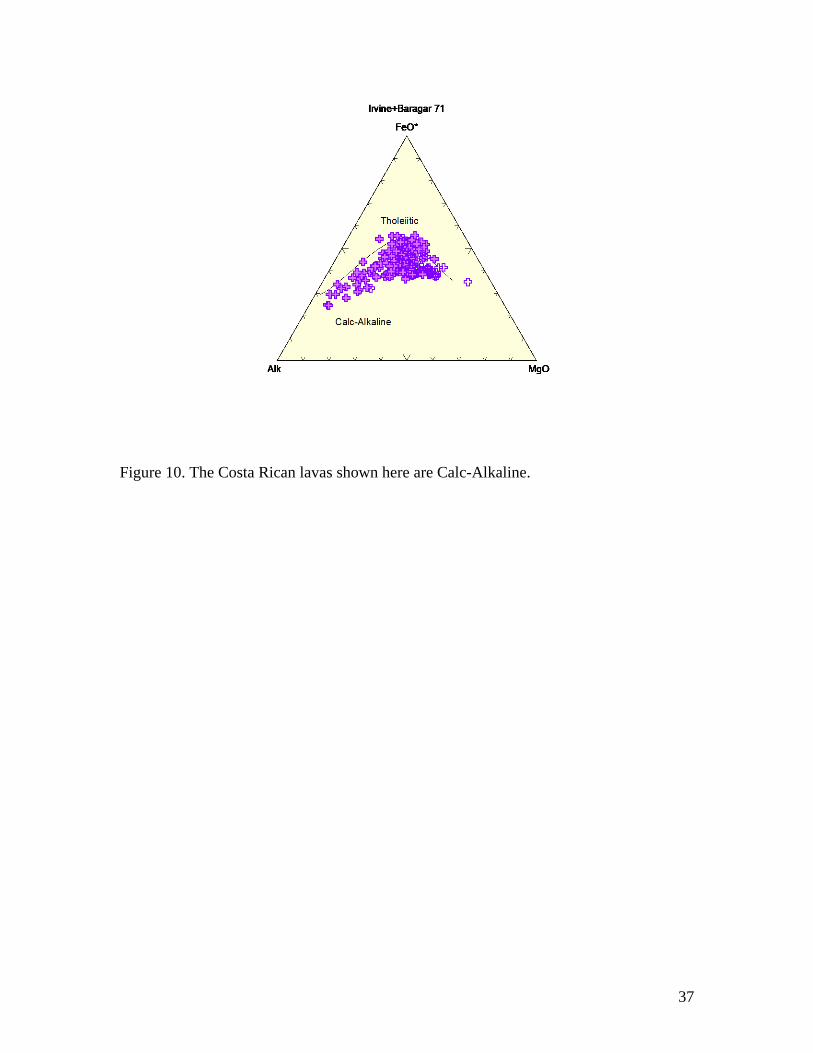
Igpet will not plot an analysis unless the OPX or CPX strings are present in the sample name. It doesn't have to be the entire name, just part of it (e.g. Sal-SA-206 cpx core). There are also mineral strings in the partition coefficient files. If the mineral sample names include the same mineral strings in both Mineral data files and partition coefficient files, Igpet will match the minerals in PC file, data files and the Mineral file definitions. One complex diagram, the Lindsley and Anderson (1983) two pyroxene geothermometer, is included. Fe++/Fe+++ is determined by charge balance in a special subroutine derived from the original publication. CMAS Projections There are many ways to transform the major elements into the four end-members, C, M, A and S. Elthon (1983) provides a lucid review and a logical projection. The textbook The Interpretation of Igneous Rocks (Cox et al., 1979) has good graphical depictions of projections. O'Hara (1976) describes the advantages of "pseudoquaternary isostructural molecular equivalent weight projections". Grove and Baker (1984) suggest that projections should be on an oxide basis, rather than a molar or weight basis. There is no agreement on how best to employ the many projections that exist. Different ones may be suitable for different circumstances. To pursue this, a good starting point is O'Hara (1976). Figure 9 is an example of a CMAS diagram. Discrimination and classification diagrams There are several groups of discrimination diagrams that attempt to define the tectonic environment of rock suites or provide useful nomenclature. Figure 10 is a typical example. Most of the discrimination diagrams are carefully reviewed in Rollinson (1993). DiscrimBasalt.txt, DiscrimGranite.txt, Komatii.txt and Mantle.txt are the files that define diagrams used for discrimination of tectonic environment. IrvineBaragar.txt contains diagrams for the Irvine and Baragar (1971) igneous rock classification scheme. Two diagram files cover the IUGS Cation NORM classification (Streckeisen and Le Maitre, 1979) and the IUGS Modal classification (Streckeisen, 1976). The first file requires adding a CIPW norm using the Barth-Niggli Cation Norm option. The second is based on petrography. It requires modal analyses from point counts or image analysis. Conclusions Igpet’s evolution suggests emphasizing the following: 1. For a given region or project, maintain a single large data file as an xls or equivalent spreadsheet data file. Edit the column headers if needed and add the 4 Igpet parameters (Sample, jcode, kcode, lcode) and then create an expendable tab delimited txt file for Igpet to read.

24

2. Aliasing allows user’s data to be in almost any order as Igpet will recognize key oxides, elements and isotope ratios needed for specialized calculations. This searching and sorting should be as transparent to the user as possible. 3. The SubSelect menu provides the sorting and selecting power needed to focus in on subsets of the large comprehensive data files. 4. Rapid data display facilitates exploration and is better achieved with button controls than via menus. 5. Different types of plots require careful modification and sometimes deactivation of the menus and buttons that comprise the user interface. 6. The most comprehensive modeling is achieved in Spider plots where all the elements plotted and their isotopic ratios are simultaneously modeled. A typical approach is to first create a source by using the Spider Mix window to mix appropriate source components. The resulting mantle composition can then be turned into a series of model melts by making several choices in the Spider Model button and subsequent window: the melt model, the mantle mode, the melt mode, the degrees of melting. The modes require a partition coefficient file that includes all the elements and mantle minerals. AFC models can further trace magmatic evolution assuming a reasonable contaminant and a partition coefficient file suitable for the P and T conditions where assimilation and fractional crystallization take place. Acknowledgements Our colleagues and semi-willing beta testers, Mark Feigenson, Claude Herzberg, Lina Patino, Karen Bemis, Fara Lindsay and many others repeatedly demonstrated uncanny ability to locate bugs within minutes of getting a "final" version of Igpet. Over the years several geoscientists have found bugs and suggested or provided useful additions. User feedback is the major way that Igpet evolved.

25

References Albarede, F., 1995, Introduction to Geochemical Modeling, Cambridge Univ. Press, New York, 543 pp. Beattie, P. (1993). Olivine–melt and orthopyroxene–melt equilibria. Contributions to Mineralogy and Petrology 115, 103–111. Blondes, M. S., P. W. Reiners, M. N. Ducea, B. S. Singer, and J. Chesley (2008), Temporal–compositional trends over short and long time-scales in basalts of the Big Pine Volcanic Field, California, Earth and Planetary Science Letters, 269(1-2), 140-154. Bottinga, Y. and Weill, D.F., 1970. Densities of liquid silicate systems calculated from partial molar volumes of oxide components. Am. J. Sci. 269:169-182 Carr MJ, Feigenson MD, Bolge LL, Walker JA, Gazel E, 2014. RU_CAGeochem, a database and sample repository for Central American volcanic rocks at Rutgers University. Geosci. Data J. (2014), doi: 10.1002/gdj3.10 Dataset: Identifier: doi:10.1594/IEDA/100409 Creator: Carr MJ, Feigenson MD, Bolge LL, Walker JA, Gazel E Title: RU_CAGeochem v.3, a database and sample repository for Central American volcanic rocks at Rutgers University Publisher: Integrated Earth Data Applications (IEDA)Publication year: 2013 Cox, K.G., Bell, J.D. and Pankhurst, R.J., 1979. The Interpretation of Igneous Rocks, Allen and Unwin, London. 450p Cross, W., Iddings, J.P., Pirsson, L.V. and H.S. Washington. 1902. A Quantitative Chemico-mineralogical Classification and Nomenclature of Igneous Rocks. J. Geol., 10:555-690. Davis, J.C. 1973. Statistics and Data Analysis in Geology. John Wiley & Sons, New York, 550 pp. DePaolo, D., 1981. Trace element and isotopic effects of combined wallrock assimilation and fractional crystallization. Earth Planet. Sci. Let., 53:189-202. Elthon, D., 1983. Isomolar and isostructural pseudo-liquidus phase diagrams for oceanic basalts. Am. Mineral. 68:506-511 Feigenson, M.D., Bolge, L.L., Carr, M.J. and Herzberg, C.T., 2003. REE Inverse Modeling of HSDP2 Basalts: Evidence for Multiple Sources in the Hawaiian Plume. Geochemistry, Geophysics, Geosystems (G3), posted 20 February 2003, 25pp.

26

Gazel, E., M. J. Carr, K. Hoernle, M. D. Feigenson, D. Szymanski, F. Hauff, and P. van den Bogaard (2009), Galapagos-OIB signature in southern Central America: Mantle refertilization by arc–hot spot interaction, Geochemistry Geophysics Geosystems, 10(2). Gazel, E., K. Hoernle, M. J. Carr, C. Herzberg, I. Saginor, P. v. den Bogaard, F. Hauff, M. Feigenson, and C. Swisher (2011), Plume–subduction interaction in southern Central America: Mantle upwelling and slab melting, Lithos, 121(1-4), 117-134. Gazel, E., T. Plank, D. W. Forsyth, C. Bendersky, C.-T. A. Lee, and E. H. Hauri (2012), Lithosphere versus asthenosphere mantle sources at the Big Pine Volcanic Field, California, Geochemistry Geophysics Geosystems, 13. Grove, T.L. and Baker, M.B., 1984. Phase equilibrium controls on the tholeiitic versus calc-alkaline differentiation trends. J. Geophys. Res. 89:3253-3274. Irvine, T.N., and Baragar, W.R.A., 1971. A guide to the chemical classification of the common volcanic rocks. Can. J. Earth Sci., 8:523-548. Johannsen, A., 1931. A Descriptive Petrography of the Igneous Rocks. Vol. I. Introduction, Textures, Classification, and Glossary. University of Chicago Press, Chicago, IL, 437 pp. Kress, V. C. & Carmichael, I. S. E. (1991). The compressibility of silicate liquids containing Fe2O3 and the effect of composition, temperature, oxygen fugacity and pressure on their redox states. Contributions to Mineralogy and Petrology 108, 82–92. Langmuir, C.H., Vocke, R.D., Hanson, G.N. and Hart, S.R., 1977. A general mixing equation: applied to the petrogenesis of basalts from Iceland and the Reykjanes Ridge. Earth Planet. Sci. Lett. 37:380-392. Langmuir, C.H., 1989. Geochemical consequences of in situ crystallization. Nature v. 340. p. 199-205. Lindsley, D.H., and Anderson, D.J., 1983. A two-pyroxene thermometer. J. Geophys. Res. 88:A887-A906. Mazza, S. E., E. Gazel, E. A. Johnson, M. J. Kunk, R. McAleer, J. A. Spotila, M. Bizimis, and D. S. Coleman (2014), Volcanoes of the passive margin: The youngest magmatic event in eastern North America, Geology, 42(6), 483-486. McDonough, W. F., and S.-s. Sun (1995), The composition of the Earth, Chemical Geology, 120, 223-253. Melson, W., O'Hearn T. and Jarosewich, 2002, A data brief on the Smithsonian Abyssal Volcanic Glass Data File, Geochemistry, Geophysics and Geosystems, 3 (4) No. 10.1029/2001GC000249.

27

O'Hara, M.J., 1976. Data reduction and projection schemes for complex compositions. in Progress in Experimental Petrology, N.E.R.C. Publication Series D, No. 6, p. 103-126. Rollinson, H., 1993. Using geochemical data: Evaluation, presentation, interpretation: Longman, Harlow, 352 pp. Saginor, I., E. Gazel, C. Condie, and M. J. Carr (2013), Evolution of geochemical variations along the Central American volcanic front, Geochemistry, Geophysics, Geosystems, 14(10), 4504-4522. Streckeisen, A. 1976. To each plutonic rock its proper name. Earth Sci. Rev. v. 12, p. 1-33. Streckeisen, A. and Le Maitre, R.W. 1979. A chemical approach ro the Modal (QAPF classification of the igneous rocks. N. Jb. Miner.Abh. v. 136 vol 2, p 169-206. Swan, A. R. H. & Sandilands, M. 1995. Introduction to Geological Data Analysis; with statistical tables by P. McCabe. Blackwell Science Oxford ; Cambridge, Mass., USA, 446 pp. Van Niekerk, H. and Von Backström J. W. 1966. A Fortran IV computer code for calculation of CIPW norms and Niggli values. Atomic Energy Board, Pelindaba, South Africa. 24 pp. Walker, D. Shibata, T. and DeLong, S.E., 1979. Abyssal tholeiites from the Oceanographer fracture zone, II-phase equilibria and mixing. Contrib. Mineral. Petrol. 70:111-125.

28

Table 1. Models available in Spider plots Model Equation coded from batch melting Albarede (1995) fractional melting “ aggregated fractional melt melting “ continuous melting “ rayleigh fractional crystallization “ equilibrium crystallization “ in situ crystallization Langmuir (1989) AFC DePaolo (1981) Mixing Albarede (1995) Recharge “ REE inverse model-CoDoPi Feigenson et al. (2003)

29

Figure 1. Igpet folders and file locations

30

Figure 2. Parameters from the CIPW cation norm define the subalkaline (tholeiitic) and alkaline fields for basalts. All the modern arc lavas of central Costa Rica are subalkaline.

Figure 3. Replication of Figure 3b from DePaolo (1981) using Igpet’s XY model tool. A single extra label was added and the option for a vertical Y-axis label was used.

31

Figure 4. An example of possible mixing among lavas from all along the Central American volcanic front. The hyperbola equation was calculated using least squares.

32

Figure 5. Use of spider diagram for evaluation of magma mixing at the Big Pine Volcanic Field, Owens Valley, California. A) Selected parental basalt (red circles) with ~10% wt% MgO and no depletions in Nb-Ta and a local rhyolite (black stars) B) Model results compared with evolved magmas (MgO <8 wt%). The parental basalt and derivative magmas are from Blondes et al. (2008), and the rhyolite composition is from the NavDat database. Pyrolite mantle normalization after McDonough and Sun (1995). The mixing models fail.

33

Figure 6. Example of Spider forward modeling to explain the composition of the incompatible element enriched Central Costa Rica lavas. A) Depleted Mantle and subduction input sources described in Gazel et la. (2009). B) Metasomatized source obtained by an optimization and forward modeling of that source at a melt fraction (F) of 8% compared to the average mafic lavas from Central Costa Rica. P does not fit because the crystallization and removal of apatite was ot included in the model.

34

Figure 7. Assessment of crustal interaction by AFC (DePaolo, 1981). Data sources in Mazza et al. (2014). All samples are corrected to the average eruptive age of the VA Eocene magmatism, ~50Ma. The blue lines represent AFC from sample TK5 using a representative crustal end-member. Every tick mark represents F=0.1, for a maximum F=1. The rate of assimilation to crystallization (R=dma/dfc) of 0.5. The black lines represent mixing between MORB and HIMU sources.

35

Figure 8. Inverse model using the primitive lavas from the Guyacan Formation from the Costa Rican back arc (Gazel et al. 2011). Sample were first corrected for fractional crystallization of olivine and then modeled following the CoDoPi model in Feigenson et al. (2003). Six models are shown and the three with the highest garnet (gt) in the input compositions fail because they generate unrealistically low calculated source concentrations and source mineralogy.

36

Figure 9. CMAS projection after Walker et al. (1979) as modified by Sack et al. (1980). Data from Masaya volcano, Nicaragua. Displaying the note at the top is optional using the NB button.

37

Figure 10. The Costa Rican lavas shown here are Calc-Alkaline.