Board of Governors of the Federal Reserve System

International Finance Discussion Papers

Number 1112

August 2014

Returns to Active Management: The Case of Hedge Funds∗

Maziar Kazemi and Ergys Islamaj

August 8, 2014

∗NOTE: International Finance Discussion Papers are preliminary materials circulated to stimulate discussionand critical comment. References to International Finance Discussion Papers (other than an acknowledgmentthat the writer has had access to unpublished material) should be cleared with the author or authors. RecentIFDPs are available on the Web at www.federalreserve.gov/pubs/ifdp/. This paper can be downloaded withoutcharge from Social Science Research Network electronic library at www.ssrn.com

Returns to Active Management: The Case of Hedge Funds1

Maziar Kazemi2 and Ergys Islamaj3

Abstract

Do more active hedge fund managers generate higher returns than their less active peers?

We attempt to answer this question. Using Kalman Filter techniques, we estimate the risk

exposure dynamics of a large sample of live and dead equity long-short hedge funds. These

estimates are then used to develop a measure of activeness for each hedge fund. Our results

show that there exists a nonlinear relationship between activeness and performance. Using raw

returns as a measure of performance, it is found that more active funds outperform the less

active ones. However, when risk adjusted returns are used to measure performance, we find

the opposite results; that is, activeness is inversely related to returns. Still, we find that a few

very active managers outperform the moderately active funds and generate higher returns. We

conclude that the most active managers use their skills to manage the riskiness of their portfolios

and are, therefore, able to provide higher risk adjusted returns. Finally, we find that compared

to the least active managers, the most active managers are less homogeneous and, therefore, due

diligence is far more important when selecting an active manager.

Keywords: Hedge Funds, Fama-French, Active Management, Dynamic Trading

JEL classifications: G11, G12, G14, G23

1The views in this paper are solely the responsibility of the author(s) and should not be interpreted as reflectingthe views of the Board of Governors of the Federal Reserve System or of any other person associated with theFederal Reserve System.

2Division of International Finance, Board of Governors of the Federal Reserve System, Washington, D.C. 20551U.S.A. Email: mazi.kazemi@frb.gov

3Department of Economics, Vassar College, Poughkeepsie, NY, 12604, U.S.A. Email: erislamaj@vassar.edu

1 Introduction

Can managers’behavior predict returns in hedge funds? Since 1997, the hedge fund industry’s

assets under management (AUM) have increased by more than 14 times, with the AUM growing

at an average pace of $100bn per year.1 Hedge funds present themselves as absolute return

investment vehicles, seeking to generate positive returns in any market condition. They can

take short positions and are not subject to the strict mandates that govern mutual funds.

Having such freedom in implementing investment strategies emphasizes the importance of the

hedge fund manager’s investment skills. Further, unlike the mutual fund industry, hedge funds

charge both management and incentive fees, where the incentive fees provide option-like returns

to managers.2. Given its loose investment mandate and fee structure, the hedge fund industry

is expected to attract the most skilled asset managers.3

This paper investigates whether more active hedge fund managers perform better than

those who are less active. Using a sample of 2,687 live and dead equity long-short hedge funds,

the Kalman Filter is employed to estimate the risk exposure dynamics of each hedge fund, which

then are used to create a measure of activeness for each fund.4 This will allow us to study the

relationship between activeness and performance.

A priori, it is not clear whether the after-fee performance of the more active funds should

exceed those of the less active funds. Fund managers that have skills in security selection may

follow a buy-and-hold approach, while those who have skills in timing various segments of the

market may follow a more active strategy. However, if both active and less active fund managers

are equally skilled, or if markets are effi cient, then because of the transaction costs, we should

expect to see lower performance on the part of the active managers.

Our primary finding is that there exists a nonlinear relationship between activeness and

performance, and that the relationship changes depending on whether raw returns or risk-

adjusted returns are used to measure performance. In general, the moderately active funds

tend to provide higher mean returns than the less active funds. But as the level of activeness

increases, the mean returns tend to decline. When risk adjusted returns are used to measure

performance, we find the opposite results. That is, the less active funds perform better than

1http://www.barclayhedge.com/research/indices/ghs/mum/Hedge_Fund.html2 In addition, most hedge fund managers have a significant portion of their personal wealth invested in the

fund, aligning their interests with those of their investors even further.3 Incentive fees are typically 20% of a fund’s profits above its previous high water mark. For instance, John Paul-

son, the founder of Paulson and Co, reportedly earned $5 billion in 2010. See http://www.forbes.com/profile/john-paulson/

4We use the four factors of Fama, French and Carhart. They are based on the performances of the marketportfolio, large vs small cap stocks, value vs growth stocks and stocks that display positive momentum vs thosethat display negative momentum.

1

the more active ones, but as the level of activeness increase, the risk-adjusted returns tend to

increase. We may conclude that the highly active funds use their skills to manage the riskiness

of their portfolios, improving the risk-return profiles of their funds. But it is less clear why, on

a risk-adjusted basis, the less active funds can perform better than the moderately active funds

when they underperform them in terms of raw returns. One can argue that the less active funds

are long-term stock pickers, and, therefore, are able to generate better risk-adjusted performance

without frequently changing their portfolios’risk exposures.

Using our measure of activeness, we create sub-samples of managers. Next, the risk-

adjusted alphas of these sub-samples are estimated. Interestingly, we find that the average

alphas for the more active sub-samples of managers are higher than those of the less active sub-

samples. However, a higher percentage of less active managers have statistically positive alphas.

This indicates that the highly active funds tend to be less homogenous than their less inactive

peers. This would suggest that due diligence and manager selection is far more important when

an investor is selecting from a group of active equity long-short managers.

Empirical studies of hedge funds performance can be broken into two broad groups. One

set of papers examine the empirical properties of the time-series of hedge fund returns. This

group of papers report mixed results regarding hedge fund managers’ abilities in generating

abnormal risk-adjusted returns.5 In particular, recent studies tend to report very low or even

negative risk-adjusted abnormal returns (i.e., alphas) for hedge funds.6

The second group of papers focuses on the impact of funds’characteristics on their relative

performance. The results show that characteristics such as size, age, location, uniqueness of

the strategy, delta of the incentive fee contract, level of co-investment by the manager and

his/her level of education may affect a fund’s performance.7 This paper adds to these findings

by reporting that cross-sectional differences in mean returns may be affected by the level of

activeness of a fund.

The relationship between how activeness and performance has been addressed by two recent

5The anecdotal and academic evidence, at least for mutual funds, is fairly clear. For example, In 2011, 84%of actively managed U.S. equity mutual funds underperformed their benchmarks. For example, see Fama andFrench (2010), Wermers (2011), andhttp://www.prnewswire.com/news-releases/84-of-actively-managed-us-equity-funds-underperformed-their-

benchmark-in-2011-57-trail-over-3-year-period-142356285.html.6See, for example, Ackermann, McEnally, and Ravenscraft (1999), Brown, Goetzmann, and Ibbotson (1999),

Agarwal and Naik (2000a, 2000b, 2000c, 2002), Capocci (2013), Edwards and Caglayan (2001), Asness, Krail, andLiew (2001), Fung and Hsieh (2000, 2001, 2004), Kao (2002), Liang (1999, 2000, 2001, 2003), Brown, Goetzmann,and Park (2000, 2001), Brown and Goetzmann (2003), Fung and Hsieh (1997, 2002, 2004), Lochoff (2002), Malkieland Saha (2005)Ding and Shawky (2007), Kosowski, Naik, and Teo (2007), Fung, Hsieh, Naik, and Ramadorai(2008), Ibbotson, Chen, and Zhu (2011), and Cao, Chen, Liang, and Lo (2013).

7See, for example, Boyson (2008), Teo (2009), Agarwal, Daniel, and Naik (2009), Li, Zhang, and Zhao (2011),Titman and Tiu (2011), Gao and Huang (2012), and Sun, Wang, and Zheng (2012).

2

papers in the case of mutual funds. To obtain their results, these studies rely on reported security

holdings. Huang, Sialm, and Zhang (2011) examine the relationship between risk-shifting and

performance. They define activeness as the difference between a fund’s prior returns variance

(over the previous 36 months) and the variance of the current holdings (in the last 36 months).

They report that funds with more stable risk level tend to perform better. Cremers and Petajisto

(2009) investigate the relationship between active share and performance. Active share is defined

as the percentage of a fund’s holdings that do not overlap with that fund’s stated benchmark

portfolio. Their results indicate that more active funds tend to perform better. This paper

differs from the above studies in two ways. First, we study hedge funds, which as discussed

before, are expected to attract the most talented traders. Second, we use reported monthly

returns as opposed to asset holdings to measure how actively each fund is managed.8 It should

be noted that the procedure developed in this paper can be applied to mutual funds as well.

This paper uses a return-based approach to estimate the exposure dynamics of our sample

of hedge funds. Wermers (2011) warns of three potential problems when conducting returns-

based performance and risk exposure analysis. First, one must have an accurate measurement of

the risk exposures of the managers by using appropriate benchmarks. Second, one must be aware

of the difference between idiosyncratic and systematic risks in the fund’s holdings. Finally, one

should have a good understanding of the return distribution, which may deviate from the normal

distribution. This paper focuses on hedge fund managers who invest in U.S. equity markets, and,

therefore, we construct a model that reflects the equity risks they take (i.e., Fama-French-Carhart

model). Second, by focusing on risk factors that have shown to affect cross-sectional differences

in equity returns, we are able to differentiate between systematic and idiosyncratic risks. Finally,

while it is assumed that hedge fund returns are normally distributed, the results are corrected

for potential heteroskedasticity when estimating the relationship between performance and our

measure of activeness.

Carhart (1997) combines the three-factor model, developed by Fama and French (1992,

1993, 1996), and the momentum factor, developed by Jegadeesh and Titman (1993). Equation

(1) represents the four-factor Fama-French-Carhart model:

rpt − rft = αp + βp(RMRFt) + sp(SMBt) + bp(HMLt) +mp(UMDt) + εpt, t = 1, ..., T. (1)

Here, rpt is the rate of return on an asset, rft is the riskless rate, RMRFt is the excess

return on the market portfolio and SMBt, HMLt and UMDt are returns to size, value and

momentum factors, respectively. Factor exposures of the asset are measured by βp, sp, bp, and

mp. Finally, the risk-adjusted performance of the investment is measured by αp.

8Funds with more than $100 million in assets have to report their long positions to the SEC. However, shortpositions are not reported.

3

Fung and Hsieh (2004) consider a seven factor model, which includes the market factor,

the size factor, and two fixed-income factors. The other three factors represent returns to look-

back options on three asset classes. The seven-factor model, in general, performs relatively

well in explaining the time-series properties of hedge funds covering a wide set of strategies.

However, this paper focuses on funds that follow equity long-short strategy in the U.S. markets.

Consequently, we use the four-factor model of Fama-French-Carhart as its factors measure the

systematic risks of the U.S. equity portfolios.

While Fung and Hsieh (2004) use look-back options to model trend-following strategies,

Hasanhodzic and Lo (2007) employ multifactor models with time varying coeffi cients to accom-

plish the same goal. The authors use a rolling-window regression to capture the dynamics of

hedge funds’investment strategies. As opposed to a constant-parameter regression, this method-

ology offers more insights into the empirical properties of hedge fund returns, but there is some

ambiguity in choosing the optimal window size. In addition, a moving window approach is based

on the assumption that coeffi cients are rather stable within each window. This paper’s objective

is similar to that of Hasanhodzic and Lo (2007), as we also are interested in estimating the

dynamics of hedge funds’exposures.

We employ the Kalman Filter approach with time-varying coeffi cients to model each hedge

fund’s return process. This allows us to obtain estimates of the time-series of each hedge fund’s

factor exposures, which are then used to create a measure of activeness for each fund. Mamaysky,

et al (2004) show that a dynamic regression using the Kalman Filter performs better in explaining

time-series properties of mutual funds’ returns and provides a more accurate out-of-sample

forecast compared to static OLS models. In the case of hedge funds, Monarcha (2009) compares

the explanatory power of a multi-factor model using the Kalman Filter with that of a static

linear model. Using a sample of 6,716 funds with monthly data from January 2003 to December

2008, Monarcha (2009) finds that the mean adjusted R2 rises from 0.60 for the static linear

model to 0.72 for the dynamic case with the Kalman Filter. Even a linear static model with

non-linear variables yields an adjusted R2 of only 0.62. Roncalli and Teiletche (2007) compare

estimates of dynamic risk exposures obtained using Kalman Filter to those obtained through a

rolling window OLS approach. They find that the Kalman Filter produces smoother estimates

of funds’factor sensitivities, and reacted to new information quicker than either the 12-month,

the 24-month, or the 36-month rolling window techniques. Bollen and Whaley (2009) use a

dynamic regression with stochastic betas to measure risk-adjusted performance of hedge funds.

They indicate that employing Kalman Filter to estimate risk exposures is an effective way to

capture the time-dynamics of hedge fund allocations.

The rest of the paper is organized as follows. The next section explains the empirical

strategy and explains the data used. Section 3 discusses results for different specifications and

4

section 4 offers some concluding remarks.

2 The Model

We use a sample of U.S. long-short equity hedge funds. The goal is to estimate each hedge

fund’s exposures to risk factors and then create a benchmark for each manager.9 Consider the

general case of the excess return on a portfolio:

rp,t − rf,t =n∑i=1

ωi,t−1(ri,t − rf,t) p = 1, ...,K (2)

In equation (2) , rp,t is the hedge fund’s returns at time t, rf,t is the risk-free rate at time t,

ωi,t−1 is the weight on asset i decided at time period t−1, and ri,t is the time t return on asset i.

The weight on risk-free rate in the portfolio is given by (1−∑ni=1 ωi,t−1). The above expression

is, in fact, an economic identity, as it describes how the excess return on a portfolio is simply a

weighted average of the excess returns of securities that constitute the portfolio.

In practice, one does not know the exact composition of the portfolio, and thus the weights

have to be estimated using available returns on a set of asset classes or risk factors that approxi-

mate the investment universe considered by the portfolio manager. Since hedge fund returns are

generally available only on a monthly basis and most hedge funds have limited track records, the

above regression cannot be estimated using a large set of asset returns as explanatory variables.

Therefore, we employ the four-factor Fama-French-Carhart model as described in equation (1)

to measure the risk exposures of each hedge fund. These four factors have been shown to rep-

resent the sources of systematic risks of equity portfolios, and they represent excess returns on

portfolios of available assets.10 Thus, the econometric representation of the model is

rp,t − rf,t = w′p,t−1ft + εp,t p = 1, ...,K, t = 1, ..., T. (3)

Here, wp,t, is a 5×1 vector of weights (i.e., factor exposures and alpha), which will be estimated

by the Kalman Filter. ft is a 5×1 vector of Fama-French-Carhart factors and the constant term.

The error term is represented by εp,t. Note that while equation (2) is an economic identity, and,

therefore, does not contain an error term, equation (3) contains an error term as it approximates

the portfolio’s return process. The weights are assumed to follow the following autoregressive

9Since the Fama-French-Carhart factors are in excess returns form, there is no need to impose a restrictionthat the weights have to add up to one. Further, since hedge funds can take long and short positions, there is noneed to impose a non-negativity restriction on weights.10For a description of all the risk-factors see http://mba.tuck.dartmouth.edu/pages/faculty/ken.french/data_library.html

5

process.

wp,t = wp,t−1 + µp,t, t = 1, ..., T,

where µp,t is a vector of normally distributed random variables with mean zero.

Once the parameters of equation (3) are estimated, we can then measure the degree of

activeness of each fund based on the variations in the estimated values of wp,t. The sum of

absolute changes in wip,t−1, where i refers to ith factor, is used to measure the activeness of each

portfolio. That is,

φp =1

Tp

4∑i=1

T∑t=2

|wip,t − wip,t−1| , p = 1, ..,K. (4)

Here φp is defined as the measure of activeness of fund p.11 Note that since our sample of hedge

fund managers have track records of different lengths, the measure of activeness is adjusted by

the length of the track record, Tp.

After the measure of activeness is obtained, we can examine the relationship between

performance and the level of activeness. We use cross-sectional regressions to determine if there

is a relationship between a hedge fund’s performance and its degree of activeness. That is, we

estimate the following regression

Zp = γ0 + γ1φp + u p = 1, ...,K (5)

Here, Zp represents the performance of hedge fund p, φp measures how actively the fund is

managed, and γi, for i = 0, 1 are the coeffi cients that have to be estimated. The hypothesis

is that γ1 ≤ 0; i.e., a higher level of activity does not lead to better performance, and due to

transaction costs, active funds tend to have lower performance compared to less active funds.

This hypothesis basically claims that U.S. equity markets are effi cient and that hedge funds

managers are not skilled enough to overcome the transaction costs and the fees associated

with managing a fund. Aknowledging the possibility of nonlinearities, we also include a square

activeness term in the regression and show the results below.

One potential problem that arises in estimating the cross-sectional regression (5) must

be noted. The explanatory variable φp is an estimate of the true measure of activeness, and,

therefore, regression (5) suffers from errors in variables. This may lead to a downward bias in

the estimated values of γ1 and γ2. We use Monte Carlo simulation to obtain estimates of the

magnitudes of the measurement errors, which are then used to adjust the estimated values of

γ1 and γ2. The details of the Monte Carlo procedure and the resulting correction are described

11The measure of activeness is similar to that of a portfolio’s turnover. Alternatively, one could use the averagestandard deviation of the time-series of the estimated weights. We decided not to use this approach because itwill not adequately capture the degree of activeness of a portfolio where the weights are trending in a predictableway.

6

in the Appendix.

We use three different measures to represent the dependent variable Zp. First, we employ

the average excess return on each manager. This will determine if the more active funds can

generate higher average net-of-fee returns. Of course, higher returns could be due to higher levels

of risk assumed by the active managers. Consequently, two different measures of risk-adjusted

excess returns, Sharpe ratio and Jensen’s alpha, are used as well.

The data is obtained from the Center for International Securities and Derivatives at the

University of Massachusetts-Amherst (CISDM). We consider 2,687 live and dead hedge funds

whose Morningstar/CISDM category is listed as U.S. Long/Short Equity. These funds invest

in U.S. stocks, taking both long and short positions. The reported monthly returns are net of

fees, calculated as the percentage change in the net asset value of each fund. The sample covers

1994-2013. We winsorized the data at the 2% level and eliminated all funds that had less than

36 months of data, but no other restrictions on whether a fund is live or dead were imposed.12

Duplicate funds were removed from the sample.

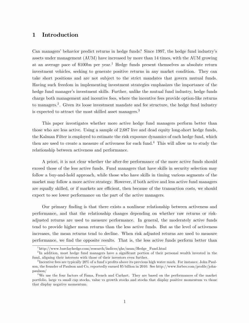
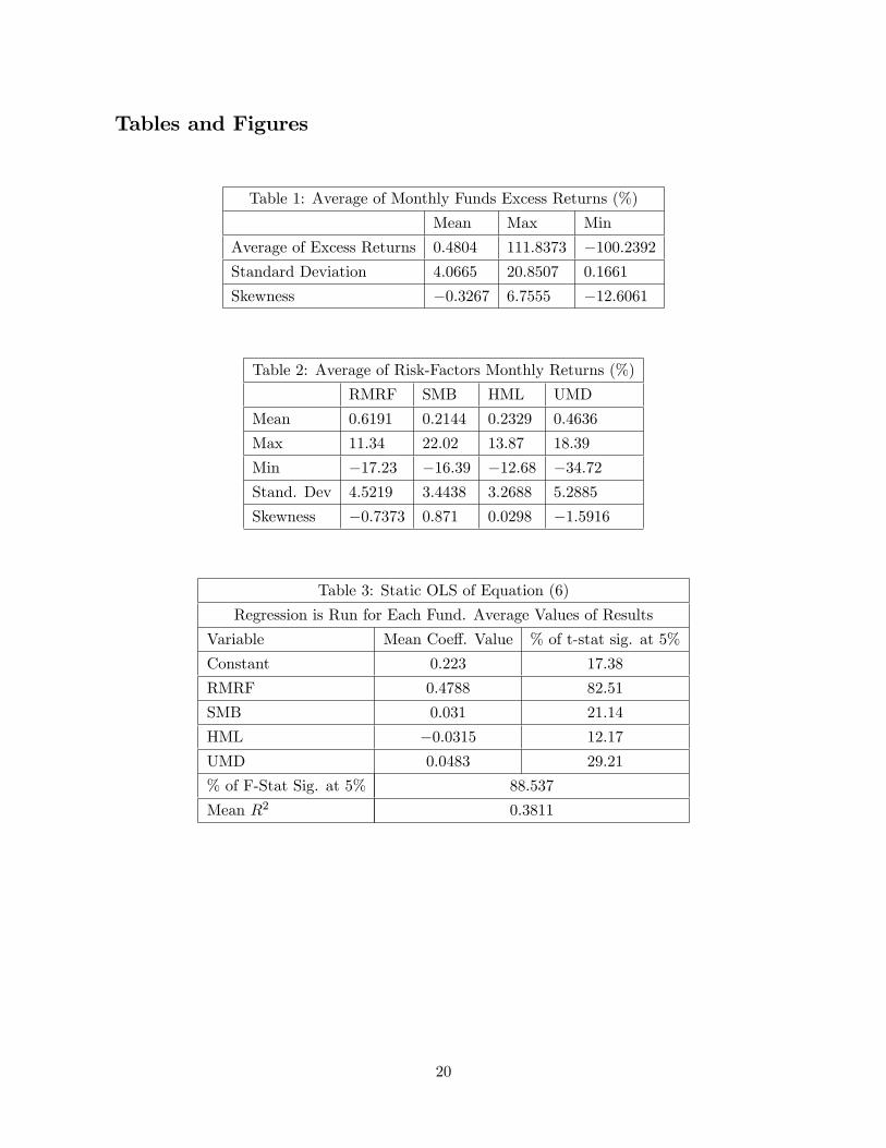
Tables 1 and 2 below present summary statistics for the funds returns, and summary

statistics for the risk-factor returns, respectively. Figure 1 shows the number of funds in our

sample. As expected, we see a large drop off in the number of funds in the middle of 2007 as

the financial crisis unfolded.

Tables 1 and 2 Here

Figure 1 Here

3 Results

3.1 Constant Coeffi cients

Before we apply the Kalman Filter, we estimate the following static OLS regression (6) using

the entire sample.

rp,t − rf,t = αp + w1p(RMRFt) + w2p(SMBt) + w3p(HMLt) + w4p(UMDt) + εt,p (6)

12The requirement that funds should have a minimum of 36 months of data may introduce survivorship and lookahead biases. Since we include dead funds in our sample, the impact of these biases on our results is mitigated.

7

This regression is the standard four-factor Fama-French-Carhart model, and was discussed in

equation (1). We begin with the static model because it is the building block of the dynamic

regression to follow. In addition, this allows us to compare our preliminary results with those

reported in previous papers. We estimate regression (6) for each manager and report the average

of the estimated coeffi cients. The results are presented in Table 3.

Table 3 Here

Note that most alphas are not significantly different from zero. In equation (6), the es-

timated mean abnormal return, αp, was 0.223% per month. Of all 2,687 funds, 467 had sig-

nificantly positive alphas at the 5% level. Since we are considering long-short equity funds, it

is not surprising that we find a high percentage of funds have significant exposure to overall

stock market risk (RMRF ). In fact, this is the only risk factor that more than 50% of funds

have significant exposure to. Consistent with previous findings, the remaining results show that

hedge funds tend to have positive exposures to the size factor, negative exposure to the value

factor and positive exposure to the momentum factor (e.g., see Capocci (2013)).

3.2 Dynamic Coeffi cients

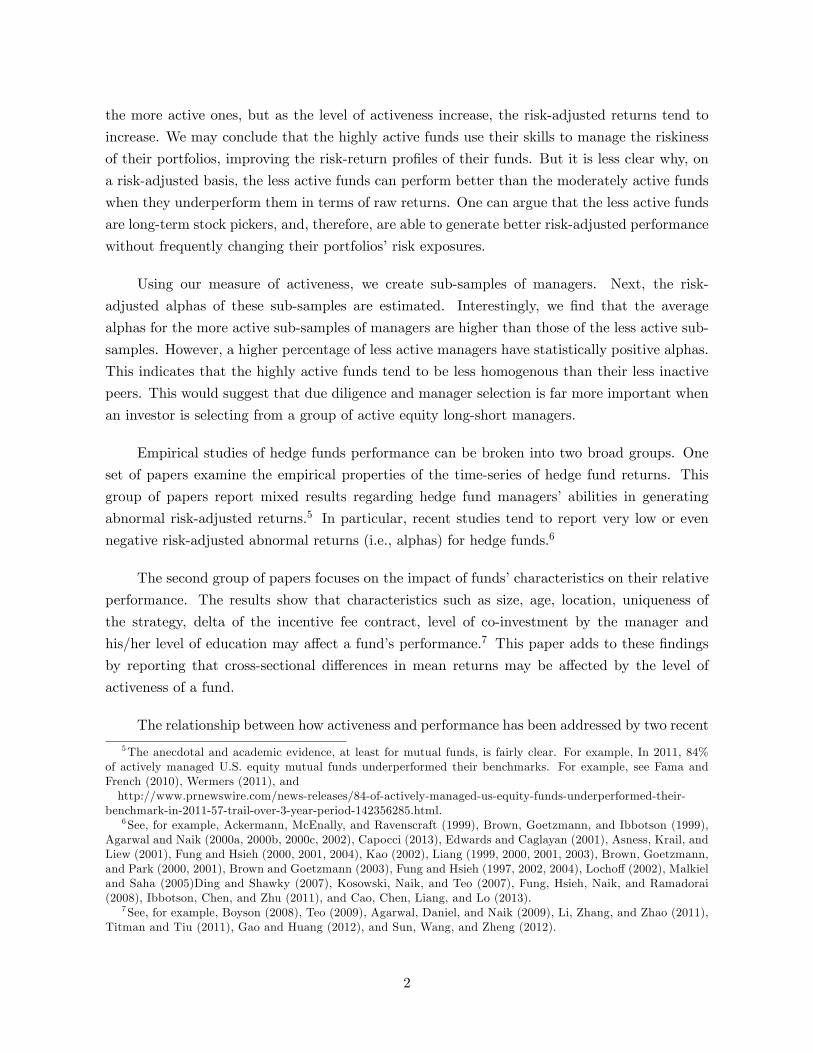
In this section, we estimate regression (6) for each manager assuming time-varying coeffi cients,

using the Kalman Filter methodology.13 Figure 2 displays the dynamics of the average estimated

weights of the four factors. It can be seen that the weights are indeed time-varying, suggesting

that fund managers actively adjust their exposures to various sources of equity risks through

time.

Figure 2 Here

The estimated time-series of each manager’s exposure to the four equity factors are, then,

used to create a measure of activeness for each manager. As described in equation (4), a

measure of activeness, φp, is constructed for each fund, which is then normalized to create a

relative measure of activeness:

ρp =φp

φ− 1,

13All empirical tests were carried out in MATLAB using the State Space Model toolbox developed by Pengand Aston (2011).

8

where φ is the mean of activeness measure for the entire sample. Therefore, ρp represents how

active fund p is relative to the average fund. A value of 0 would indicate that a fund’s level

of activity is average, while a positive (negative) value means the manager is more (less) active

than average. Observing this measure of activeness, we see that there are a handful of managers

with extremely high levels of activeness (orders of three times the average activeness). Thus, we

eliminate these outliers and consider only funds who have a value of ρp less than three. We do

not find the same extreme outliers for negative values of ρp (i.e. less active funds). We are left

with 2,674 managers.14

3.3 Sorting Results

Before estimating our cross-sectional regressions, some preliminary results are presented by

sorting the entire sample into sub-samples consisting of the highly active and less active funds.

We use the top (bottom) 5, 10 and 25 percent to create samples of the most (least) active

funds. Table 4 presents the summary statistics for excess returns and activeness in each group.

A t-test for the difference in means shows that the average excess returns of the most active

funds are statistically higher than those of the least active funds. In addition, the highly active

funds’returns are more volatile than the returns of least active ones. Finally, while the most

active funds tend to have higher skewness than the least active funds, all have roughly the

same kurtosis. It important to note that the mean returns on the least active funds do not

increase monotonically as activeness increases. This indicates that there may exist a non-linear

relationship between performance and activeness.

Next, the same sub-samples of the most active and the least active funds are used to run

the Fama-French-Carhart model with constant coeffi cients. The results, which are presented in

Table 5, clearly suggest that the most active funds tend to have, on average, higher alphas than

the least active funds. We see that compared to the least active funds, the most active funds

tend to have higher exposures to the market and the size factors, and similar exposures to the

value and the momentum factors. Finally, similar to the results reported in Table 4, we see that

the relationship between alpha and activeness is not monotonic, reinforcing the idea that the

relationship might be non-linear.

The higher exposure to the size factor is surprising because the bid-ask spread and price

impact are larger for small cap stocks, which imposes higher costs on active managers. If,

despite these added costs, these managers were able to produce higher returns than their less

active peers, then the argument that active managers are more skilled than their less active

peers would be strengthened.14The results are similar for the whole sample.

9

Finally, results reported in Table 5 show that a much higher percentage of less active funds

have statistically positive alphas. That is, while the average alphas of the active sub-samples

are higher, fewer of those active managers have positive alphas. As mentioned, the most active

managers have to overcome the higher levels of transactions costs, and, therefore, only those

who are highly skilled can offer higher risk-adjusted returns; these results indicate that only a

small group of equity long-short managers posses that level of skill.

Tables 4 and 5 Here

3.4 Regressions Using Raw Returns

Three cross-sectional regressions using our measure of activeness are estimated. First, we run

regression equation (5) where the independent variable is the mean excess return of the fund.

The regression employs White estimates of the variance covariance matrix of errors to correct

for heteroskedasticity.15 Also, throughout the paper, the estimated coeffi cients are corrected for

errors in variables using the process described in the Appendix. Table 6 presents the results of

this regression.

Table 6 Here

Table 6 presents two sets of results. Column (a) represents the cross-sectional results when

activeness appears only in the linear form, while Column (b) includes the squared value of the

activeness measure as well. We find that, γ1, the coeffi cient on the measure of activeness is

statistically significant and greater than zero at the 5% level. The result indicates that the more

active funds tend to generate higher mean return. The results obtained from sorting our sample

seemed to indicate that performance has a nonlinear relationship with activeness, and the figures

appearing in Column (b) confirm this. We can see that γ2 is negative and significant at 5%

level. These findings indicate that the highly active or inactive funds tend to underperform the

moderately active funds. The cut-off point, though, is close to a measure of activeness equal

to 10, which is unrealistic for our sample. But, the relationship seems to support the idea that

15Given an n × n regressor matrix, X, and OLS residual ui for each observation, White’s estimated variance-covariance matrix for β is,

V ar[β]=(X′X

)−1X′diag

(u21...u

2n

)X(X′X

)−1See Greene (2011).

10

too much activeness will be associated with lower returns due to higher transaction costs. In

the absence of significant differences in skills, we should expect to see lower average returns

on the most actively managed portfolios. However, the cut-off seems to be above the range of

available estimates of managers’behavior and transaction costs cannot explain why the least

active funds tend to underperform the moderately active funds. This may lead us to conclude

that moderately active fund managers are highly skilled compared to their less active peers. Of

course, there is an alternative explanation: fund managers that are somewhat active tend to

assume more risks, and this how they are able to generate higher returns.

3.5 Regressions Using Risk-Adjusted Returns

To explore the possibility that higher risk is responsible for higher mean returns offered by

the moderately active funds, we re-estimate equation (5), using each fund’s Sharpe ratio and

Jensen’s alpha as the dependent variables.16 Jensen’s alpha refers to the average value of the

intercept in equation (1) with the factor exposures estimated using the Kalman Filter, and the

Sharpe ratio, SRp, refers to (rp − rf ) /σp, where rp is the mean return on fund p, rf is the

riskless rate and σp is the standard deviation of return on fund p.

The results of estimating equation (5) when Zp = SRp are presented in Table 7.

Table 7 Here

Again, similar to previous section we present both the estimation results for both the linear

and non-linear equations. Column (a) of Table 7 shows that there exists a statistically significant

negative relationship between activeness and the Sharpe ratio, although column (a) suggest that

the estimate is very close to zero. Column (b) suggests that funds with an activeness level of

above 2.4 generate higher returns that the less active ones. Previously, we reported higher mean

return on the moderately active funds. Therefore, the above results indicate that returns to

the moderately active funds are more volatile than those of the less active funds. Further, the

increase in volatility is not commensurate with higher return leading to lower Sharpe ratios for

the moderately active funds. The coeffi cient of the measure of activeness squared is positive and

highly significant. This indicates that while the moderately active funds fail to generate higher

Sharpe ratios compared to their less active peer, the highly active funds are able to increase

their Sharpe ratios.

16For a discussion of the Sharpe ratio see Sharpe (1994).

11

This is surprising because we saw in the previous section that the mean returns on the

highly active funds tend to be lower than those of the moderately active funds, while the results

appearing in Table 7 indicate that the same managers are able to generate higher Sharpe ratios

than moderately active funds. We may conclude that the highly active managers tend to be

more skilled in managing the risk of their portfolios. The question that arises is whether these

managers are skilled in managing both the total and the systematic risks of their portfolios.

Sharpe ratio adjusts returns for the total risk of a portfolio’s return, while investors may

demand compensation only for the systematic risk of the portfolio. To account for the systematic

risk of each fund, we examine the relationship between its mean alpha and its level of activeness.

We estimate equation (5) with the mean alpha of each fund as the independent variable, where

mean alpha is estimated from the time-series of alphas generated by the dynamic four-factor

model. The results are presented in Table 8. We report our findings for both linear and nonlinear

cases.

Table 8 Here

Looking at Column (a), we see that the estimated value of γ1 is negative and highly

significant. Similar to the results obtained when Sharpe ratio was used to measure performance,

this indicates that the moderately active funds tend to generate lower alphas than the less active

funds. For the non-linear case, γ1 is still negative and significant, while γ2 is positive and highly

significant. The cut-off is similar to the one in Table 7 and corresponds to a level of activeness

of approximately 2.4. Again, similar to the previous results, we can see that the highly active

funds are able to generate higher alphas than the moderately active funds.

Results of Tables 7 and 8 indicate that while, on a risk-adjusted basis, the less active funds

tend to perform better than the moderately active funds, there are some highly active funds

that could generate higher risk-adjusted returns. Further, we can conclude that most active

fund managers do not have the skills to manage the risks generated by their trading strategies

and that they tend to underperform their less active peers on a risk adjusted basis.

3.6 Live versus Dead Funds

Since our data consists of live and dead funds, we are, naturally, interested to see if the rela-

tionships between activeness and performance is the same for live and dead funds. One would

expect that if our sample is restricted to include only “live”funds, a stronger positive relation-

ship between activeness and performance will be observed. It may be that active managers who

12

survive perform better than inactive managers that survive. We re-estimated the cross-section

regressions of the last section for dead funds and live funds separately. For the purpose of this

section, a fund is considered dead if it has no returns data in our database for the last 12 months.

A fund is considered live if it has at least 60 months of data and has reported returns for the last

12 months. This leaves us with 1,588 dead funds and 789 live funds. We find almost identical

results as in the full sample. The only differences are that we do not find a significant coeffi cient

on activeness squared for live funds in the regression with alpha as a dependent variable. We

also do not find evidence of non-linearities for dead funds when we consider the raw returns

regression. We hypothesize that this is a time period specific phenomenon. We see that there

is a sharp dropoff in the number of funds after the middle of 2007. Thus we divide our sample

into the first 160 months and the last 80 months. We find a sharp contrast: The mean return

for fund managers in the earlier sample is 0.9434%, while for the second sample it is −0.0396.

Thus, the market environment was more favorable in the pre-2007 period. The results for live

managers are the same as the full sample results when we restrict ourselves to the first time

period. Similarly, non-linearities are found for dead funds when we consider the latter time

period. Since, by definition, live funds have been functioning more recently than dead ones, we

believe that these subsample regressions confirm our time dependence hypothesis. 17

4 Conclusion

Do active hedge fund managers perform better than their less active peers? We use a sample

of 2,687 U.S. equity long-short hedge funds covering 1994-2013, to answer this question. The

Kalman Filtering approach is applied to this sample in order to estimate the dynamics of each

fund’s exposure to Fama-French-Carhart factors. The time-series of these exposures are then

used to create a measure of activeness for each fund. Finally, using cross-sectional regressions

we attempt to answer the question posed above.

The empirical evidence presented in this paper shows that there is a nonlinear relationship

between performance and the measure of activeness. Interestingly, this relationship changes

depending on whether raw returns or risk-adjusted returns are used to measure performance.

When raw returns are used as performance measure, we find that the moderately active

funds tend to outperform the less active funds. However, as the level of activeness increases, the

performance of the active funds declines. The returns in this industry seem to dwarf the higher

transaction costs associated with actively managed portfolios for plausible levels of activeness

17We also estimated our cross-sectional regressions with AUM included as a control variable. Our sample wassmaller in this case as we do not have AUM data for all the funds. However, there was no qualitative change inthe results. All coeffi cients remained significant and their signs did not change.

13

and more active funds generate higher raw returns than their less active peers. Alternatively,

we can interpret the results that the active funds have riskier investment strategies. To find

out whether skill or risk is the reason for the higher return by the moderately active funds, we

repeat the above analysis, but this time we use Sharpe ratios and Jensen’s alpha as measures of

performance. Our results show that the less active funds perform better than the moderately

active funds on a risk adjusted basis. However, as the level of activeness increases, then at some

point, the risk-adjusted returns of a few highly active funds begin to improve. The above results

are robust and hold for both dead and live funds. In addition, when size is added as a control

variable, the results remain virtually the same.

Another finding of this paper is that the least active funds tend to be more homogenous

compared to their most active peers. While, on average, sub-samples of the active funds may

have higher risk-adjusted returns than the sub-samples of the least active funds, lower percentage

of the active managers have positive alphas. This indicates that only a small group of the most

active managers posses the skills to overcome the higher transaction cost and provide positive

risk-adjusted alphas. The implication for investors is that they need to spend more resources

on due diligence and manager selection when considering active equity long-short managers.

14

5 Appendix

Consider equation (5) of the text

Zp = γ0 + γ1φp + ε p = 1, ...,K

which will suffer from errors in variables as the measure of activeness has to be estimated.

Here, we briefly describe our method for correcting out estimated coeffi cients for the presence

of measurement error in independent variable. In general, it can be shown that18,

plim γ1 ×((φ′pφp

)−1 (φ′pφp + u′u

))= γ1

Here, γ is the biased estimate of the true γ when equation (5) is used. φp is a matrix of the true

values of the independent variable, and u is a matrix of measurement errors that are independent

of φp, the error term of the regression, and the dependent variable of the regression. Since we

cannot observe the true value of φp, we estimate the adjustment matrix via simulation. We

generate random exposures with means and volatilities that fall within the range of means and

volatilities estimated for our sample. These random exposures are then used to generate the

return on portfolio that invests the four factors. Using the same procedure that is employed

to estimate hedge fund managers measure of activeness, the same measure is estimated for the

simulated portfolio. Finally, the estimated value of the activeness measure is compared to its

actual value. This procedure is repeated 1000 times, which allows us to obtain an estimate of((φ′pφp

)−1 (φ′pφp + u′u

)).

The value of this adjustment factor is used to remove the bias from the estimated value of γ1.

18For a discussion of errors in variables see Greene (2011).

15

References

[1] Ackermann, Carl, McEnally, Mark, and David Ravenscraft. 1999. "The Performance of

Hedge Funds: Risk, Return, and Incentives". Journal of Finance. 54(3), 833-874

[2] Agarwal, Vikas and Narayan Y. Naik. 2000a. "Generalized Style Analysis of Hedge Funds".

Journal of Asset Management. 1, 93-109

[3] Agarwal, Vikas and Narayan Y. Naik. 2000b. "Multi-Period Performance Persistence Analy-

sis of Hedge Funds". Journal of Financial and Quantitative Analysis. 35, 327-342

[4] Agarwal, Vikas and Narayan Y, Naik. 2000c. "On Taking the Alternative Route: Risk, Re-

wards, and Performance Persistence of Hedge Funds". Journal of Alternative Investments.

2(4), 6-23

[5] Agarwal, Vikas and Narayan Y. Naik. 2002. "Determinants of Money-Flow and Risk-Taking

Behavior in the Hedge Fund Industry". Working Paper, Georgia State University

[6] Agarwal, Vikas, Daniel, N. D., and Narayan Y. Naik. 2009. "Role of Managerial Incentives

and Discretion in Hedge Fund Performance". Journal of Finance. 64, 2221-2256

[7] Asness, Clifford, Krail, Robert, and Liew, John. 2001. "Do Hedge Funds Hedge?". Journal

of Portfolio Management, 28(1), 6-20

[8] Bollen, Nicholas P. B., and Robert E. Whaley. 2009. "Hedge Fund Risk Dynamics: Impli-

cations for Performance Appraisal." Journal of Finance, 64(2), 985-1035

[9] Boyson, Nicole M. 2008. "Hedge Fund Performance Persistance: A New Approach." Finan-

cial Analysts Journal. 64(6), 27-44

[10] Brown, Stephen J. and William N. Goetzmann. 2003. "Hedge Funds with Style". Journal

of Portfolio Management. 29, 101-112

[11] Brown, Stephen J., Goetzmann, William N., and J. Park. 2001. "Careers and Survival:

Competition and Risk in the Hedge Fund and CTA Industry". Journal of Finance. 56,

1869-1886

[12] Brown, Stephen J., Goetzmann, William N., and J. Park. 2000. "Hedge Funds and the

Asian Currency Crisis". Journal of Portfolio Management. 26(4), 95-101

[13] Brown, Stephen J., Goetzmann, William N., and Roger G. Ibbotson. 1999. "Offshore Hedge

Funds: Survival & Performance 1989-1995". Yale Working Paper Series

[14] Capocci, Daniel P. J. 2013, "The Complete Guide to Hedge Funds and Hedge Fund Strate-

gies," Palgrave Macmillan.

16

[15] Cao, C., Chen, Y., Liang, B., and A. Lo. 2013. "Can Hedge Funds Time Market Liquidity?".

Journal of Financial Economics. 109(2), 493-516

[16] Carhart, Mark M. 1997. "On Persistence in Mutual Fund Performance". Journal of Finance,

52(1), 57-82

[17] Cremers, K. J. Martijn, and Antti Petajitso. 2009. "How Active Is Your Fund Manager? A

New Measure that Predicts Performance". The Review of Financial Studies. 22(9), 3329-

3365

[18] Ding, Bill, and Hany A. Shawky. 2007. "The Performance of Hedge Fund Strategies and

the Asymmetry of Return Distributions". European Financial Management. 13(2), 309-331

[19] Edwards, Franklin, and M. Caglayan. 2001. "Hedge Fund Performance and Manager Skill".

Journal of Futures Market. 21(11), 1001-1028

[20] Fama, Eugene F., and Kenneth R. French. 1992. "The Cross-Section of Expected Stock

Returns". Journal of Finance. 47(2), 427-465

[21] Fama, Eugene F., and Kenneth R. French. 1993. "Common Risk Factors in the Returns on

Stocks and Bonds". Journal of Financial Economics. 33(1), 3-56

[22] Fama, Eugene F., and Kenneth R. French. 1996. "Multifactor Explanations of Asset Pricing

Anomalies". Journal of Finance. 51(1), 55-84

[23] Fama, Eugene F., and Kenneth R. French. 2010. "Luck Versus Skill in the Cross Section of

Mutual Fund Returns." Journal of Finance. 65(5), 1915-1947

[24] Fung, William, and David A. Hsieh. 2002. "Asset-Based Style Factors for Hedge Funds".

Financial Analysts Journal. 58(5), 16-27

[25] Fung, William, and David A. Hsieh. 1997. "Empirical Characteristics of Dynamic Trading

Strategies: The Case of Hedge Funds". Review of Financial Studies. 10, 275-302

[26] Fung, William and David A. Hsieh. 2000. "Performance Characteristics of Hedge Funds

and CTA Funds: Natural Versus Spurious Biases". Journal of Financial and Quantitative

Analysis. 35, 291-307

[27] Fung, William, and David A. Hsieh. 2001. "The Risk in Hedge Fund Strategies: Theory

and Evidence from Trend Followers". The Review of Financial Studies. 14(2), 313-341

[28] Fung, William, and David A. Hsieh. 2004. "Hedge Fund Benchmarks: A Risk-Based Ap-

proach". Financial Analysts Journal. 60(5), 65-80

[29] Fung, William, Hsieh, David A., Naik, N., and T. Ramadorai. 2008. "Hedge Funds, Perfor-

mance, Risk, and Capital Formation". Journal of Finance. 64. 1777-1803.

17

[30] Gao, M. and J. Huang. 2012. "Capitalizing on Capitol Hill: Informed Trading by Hedge

Fund Managers". National University of Singapore Working Paper

[31] Hasanhodzic, Jasmina, and Andrew W. Lo. 2007. "Can Hedge-Fund Returns Be Repli-

cated?: The Linear Case". Can Hedge-Fund Returns Be Replicated?: The Linear Case"

Journal of Investment Management, Vol. 5, No. 2, pp. 5-45

[32] Greene, William H. 2011, Econometric Analysis, Prentice-Hall, New York.

[33] Huang, Jennifer, Sialm, Clemens, and Hanjiang Zhang. 2011. "Risk Shifting and Mutual

Fund Performance". The Review of Financial Studies. 24(8), 2575-2616

[34] Ibbotson, R.G., Chen, P., and K. X. Zhu. 2011. "The ABCs of Hedge Funds: Alphas, Betas,

and Costs". Financial Analysts Journal. 67, 15-25

[35] Jegadeesh, Narasimhan, and Sheridan Titaman. 1993. "Returns to Buying Winners and

Selling Losers: Implications for Stock Market Effi ciency". Journal of Finance. 48(1), 65-91

[36] Kao, D. 2002. "Battle for Alphas: Hedge Funds Versus Long-Only Portfolios". Financial

Analysts Journal. 58(2), 16-34

[37] Kosowski, R., Naik, N., and M. Teo. 2007. "Do Hedge Funds Deliver Alpha? A Bayesian

and Bootstrap Analysis". Journal of Financial and Quantitative Analysis. 31, 3291-3310

[38] Li, H., Zhang, X., and R. Zhao. 2011. "Investing in Talents: Manager Characteristics and

Hedge Fund Performances". Journal of Financial and Quantitative Analysis. 46, 59-82

[39] Liang, Bing. 1999. "On the Performance of Hedge Funds". Financial Analysts Journal. 55,

72-85

[40] Liang, Bing. 2000. "Hedge Funds: The Living and the Dead". Journal of Financial and

Quantitative Analysis. 35, 309-326

[41] Liang, Bing. 2001. "Hedge Fund Performance: 1990-1999". Financial Analysts Journal. 57,

11-18

[42] Liang, Bing. 2003. "The Accuracy of Hedge Fund Returns". Journal of Portfolio Manage-

ment. 29, 111-122

[43] Lochoff, R.W. 2002. "Hedge Funds and Hope". Journal of Portfolio Management. 28(4),

92-99.

[44] Malkiel, B. and A. Saha. 2005. "Hedge Funds: Risk and Return". Financial Analysts Jour-

nal. 61. 80-88

18

[45] Mamaysky, H.,Spiegel, M., and H. Zhang. 2004, "Estimating the Dynamics of Mutual Fund

Alphas and Betas". Yale IFC Working Paper

[46] Monarcha, Guillaume. 2009. "A Dynamic Style Analysis Model for Hedge Funds". Orion

Financial Partners Working Paper Series

[47] Peng, Jyh-Ying, and John A. D. Ashton. 2011. "The State Space Models Toolbox for

MATLAB". Journal of Statistical Software, 41(6)

[48] Roncalli, Thierry, and Jerome Teıletche. 2007. "An Alternative Approach to Alternative

Beta". Working Paper Series

[49] Sharpe, William F. 1994, "Sharpe Ratio," The Journal of Portfolio Management, 21(1).

[50] Sun, Z., Wang, A. and L. Zhang. 2012. "The Road Less Traveled: Strategy Distinctiveness

and Hedge Fund Performance". Review of Financial Studies. 25(1), 96-143

[51] Teo, M. 2009. "The Geography of Hedge Funds". Review of Financial Studies. 22, 3531-3561

[52] Titman, S., and C. Tiu. 2011. "Do the Best Hedge Funds Hedge". Review of Financial

Studies. 24, 123-168

[53] Wermers, Russ. 2011. "Performance Measurement of Mutual Funds, Hedge Funds, and

Institutional Accounts". Annual Review of Financial Economics, 3, 537-574

19

Tables and Figures

Table 1: Average of Monthly Funds Excess Returns (%)

Mean Max Min

Average of Excess Returns 0.4804 111.8373 −100.2392

Standard Deviation 4.0665 20.8507 0.1661

Skewness −0.3267 6.7555 −12.6061

Table 2: Average of Risk-Factors Monthly Returns (%)

RMRF SMB HML UMD

Mean 0.6191 0.2144 0.2329 0.4636

Max 11.34 22.02 13.87 18.39

Min −17.23 −16.39 −12.68 −34.72

Stand. Dev 4.5219 3.4438 3.2688 5.2885

Skewness −0.7373 0.871 0.0298 −1.5916

Table 3: Static OLS of Equation (6)

Regression is Run for Each Fund. Average Values of Results

Variable Mean Coeff. Value % of t-stat sig. at 5%

Constant 0.223 17.38

RMRF 0.4788 82.51

SMB 0.031 21.14

HML −0.0315 12.17

UMD 0.0483 29.21

% of F-Stat Sig. at 5% 88.537

Mean R2 0.3811

20

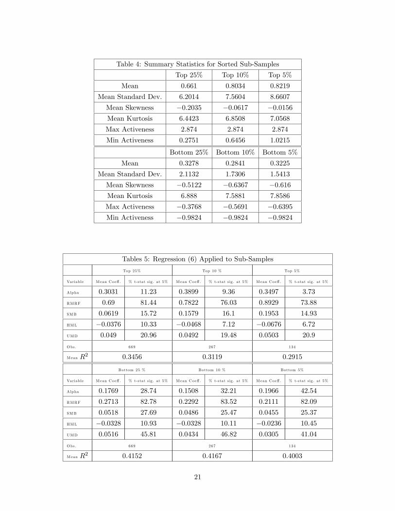
Table 4: Summary Statistics for Sorted Sub-Samples

Top 25% Top 10% Top 5%

Mean 0.661 0.8034 0.8219

Mean Standard Dev. 6.2014 7.5604 8.6607

Mean Skewness −0.2035 −0.0617 −0.0156

Mean Kurtosis 6.4423 6.8508 7.0568

Max Activeness 2.874 2.874 2.874

Min Activeness 0.2751 0.6456 1.0215

Bottom 25% Bottom 10% Bottom 5%

Mean 0.3278 0.2841 0.3225

Mean Standard Dev. 2.1132 1.7306 1.5413

Mean Skewness −0.5122 −0.6367 −0.616

Mean Kurtosis 6.888 7.5881 7.8586

Max Activeness −0.3768 −0.5691 −0.6395

Min Activeness −0.9824 −0.9824 −0.9824

Tables 5: Regression (6) Applied to Sub-Samples

Top 25% Top 10 % Top 5%

Variab le M ean Coeff. % t-stat sig . at 5% Mean Coeff. % t-stat sig . at 5% Mean Coeff. % t-stat sig . at 5%

Alpha 0.3031 11.23 0.3899 9.36 0.3497 3.73

RMRF 0.69 81.44 0.7822 76.03 0.8929 73.88

SMB 0.0619 15.72 0.1579 16.1 0.1953 14.93

HML −0.0376 10.33 −0.0468 7.12 −0.0676 6.72

UMD 0.049 20.96 0.0492 19.48 0.0503 20.9

Obs. 669 267 134

M ean R2 0.3456 0.3119 0.2915

Bottom 25 % Bottom 10 % Bottom 5%

Variab le M ean Coeff. % t-stat sig . at 5% Mean Coeff. % t-stat sig . at 5% Mean Coeff. % t-stat sig . at 5%

Alpha 0.1769 28.74 0.1508 32.21 0.1966 42.54

RMRF 0.2713 82.78 0.2292 83.52 0.2111 82.09

SMB 0.0518 27.69 0.0486 25.47 0.0455 25.37

HML −0.0328 10.93 −0.0328 10.11 −0.0236 10.45

UMD 0.0516 45.81 0.0434 46.82 0.0305 41.04

Obs. 669 267 134

M ean R2 0.4152 0.4167 0.4003

21

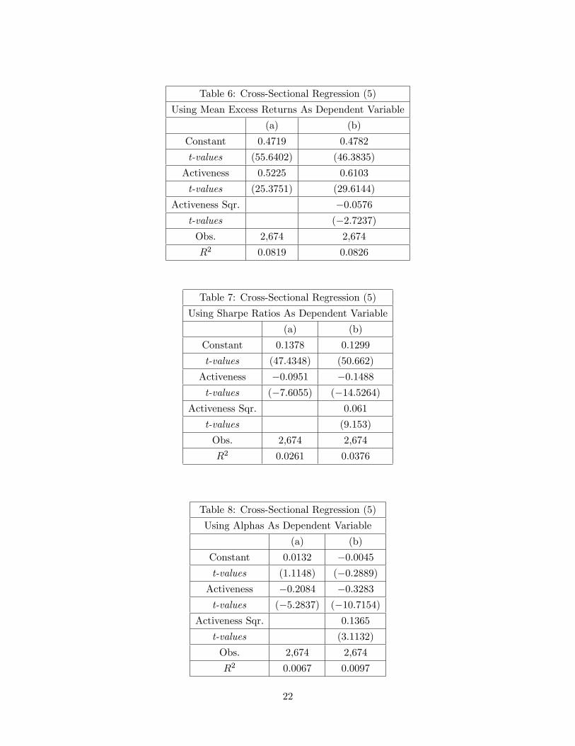
Table 6: Cross-Sectional Regression (5)

Using Mean Excess Returns As Dependent Variable

(a) (b)

Constant 0.4719 0.4782

t-values (55.6402) (46.3835)

Activeness 0.5225 0.6103

t-values (25.3751) (29.6144)

Activeness Sqr. −0.0576

t-values (−2.7237)

Obs. 2,674 2,674

R2 0.0819 0.0826

Table 7: Cross-Sectional Regression (5)

Using Sharpe Ratios As Dependent Variable

(a) (b)

Constant 0.1378 0.1299

t-values (47.4348) (50.662)

Activeness −0.0951 −0.1488

t-values (−7.6055) (−14.5264)

Activeness Sqr. 0.061

t-values (9.153)

Obs. 2,674 2,674

R2 0.0261 0.0376

Table 8: Cross-Sectional Regression (5)

Using Alphas As Dependent Variable

(a) (b)

Constant 0.0132 −0.0045

t-values (1.1148) (−0.2889)

Activeness −0.2084 −0.3283

t-values (−5.2837) (−10.7154)

Activeness Sqr. 0.1365

t-values (3.1132)

Obs. 2,674 2,674

R2 0.0067 0.0097

22

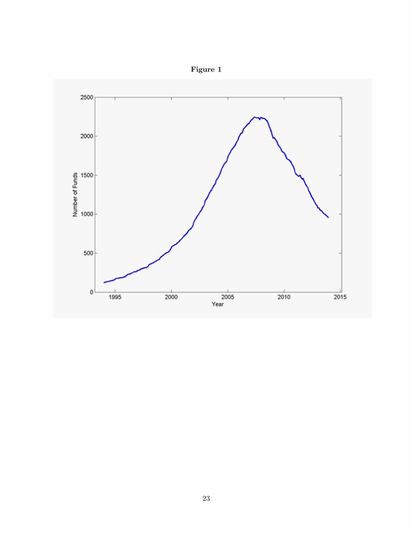
Figure 1

23

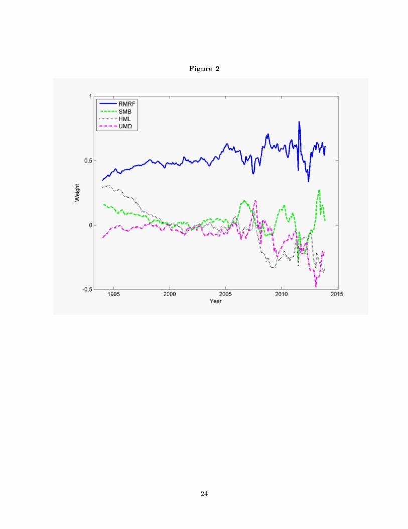
Figure 2

24