MB0048 –Operations ResearchAssignment Set- 2

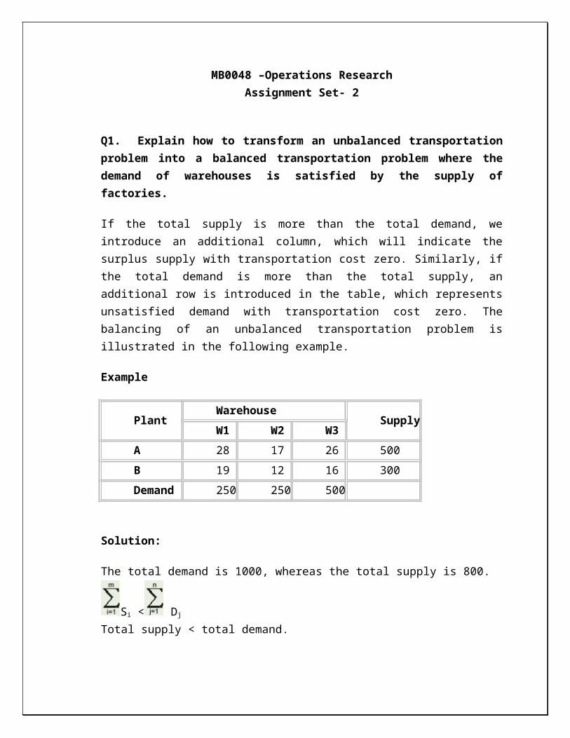
Q1. Explain how to transform an unbalanced transportation problem into a balanced transportation problem where the demand of warehouses is satisfied by the supply of factories.

If the total supply is more than the total demand, we introduce an additional column, which will indicate the surplus supply with transportation cost zero. Similarly, if the total demand is more than the total supply, an additional row is introduced in the table, which represents unsatisfied demand with transportation cost zero. The balancing of an unbalanced transportation problem is illustrated in the following example.

Example

PlantWarehouse

Supply W1 W2 W3

A 28 17 26 500

B 19 12 16 300

Demand 250 250 500

Solution:

The total demand is 1000, whereas the total supply is 800.

Si < Dj Total supply < total demand.To solve the problem, we introduce an additional row with transportation cost zero indicating the unsatisfied demand.

PlantWarehouse

Supply W1 W2 W3

A 28 17 26 500

B 19 12 16 300

Unsatisfied 0 0 0 200

demand

Demand 250 250 500 1000

Using matrix minimum method, we get the following allocations.

PlantWarehouse

Supply W1 W2 W3

A 17 500

B 19 300

Unsatisfied demand

0 0 200

Demand 250 250 500 1000

Initial basic feasible solution

50 X 28 + 450 X 26 + 250 X 12 + 50 X 16 + 200 X 0 = 16900.

2. Explain how the profit maximization transportation problem into a balanced transportation problem where the demand of warehouses is satisfied by the supply of factories

A firm has three factories located in city A, B & C and supplies goods to four dealers, dealer 1, 2, 3 & 4, spread all over the country. The production capacities of these factories are 1000, 700 & 900 units per month respectively. The monthly orders from the dealers are 900, 800, 500 & 400 units respectively. Per unit return (excluding transportation costs) are Rs. 8, 7 & 9 at the three factories. Unit transportation costs from the dealers are given below:

Factory Dealers

1 2 3 4

City - A 2 2 2 4

City - B 3 5 3 2

City - C 4 3 2 1

Optimal distribution system to maximize the total r eturn to be determined.

From the given data, we compute a matrix of net returns as done in table below;(Transportation matrix (Net return) for the Maximization problem)

Factory Dealers Factory capacity1 2 3 4

City - A 6 6 6 4 1000

City - B 4 2 4 5 700

City - C 5 6 7 8 900

To convert the given maximization problem to an equivalent minimization problem, we identify the cell (element) which has the highest contribution per unit (in this problem C-4 has highest per unit contribution, Rs.8), and subtract all elements from this highest element. The resultant matrix is a transportation problem with minimizing objective function. This has been given in the following table.

(Transportation matrix for the Minimization problem)

Factory Dealers Factory capacity1 2 3 4

City - A 2 2 2 4 1000

City - B 4 6 4 3 700

City - C 3 2 1 0 900

Dealer requirement

900 800 500 400 2600

The minimization problem is solved as a usual transportation problem. The resulting optimal solution is also the optimal solution to the original (maximization) problem. The value of the objective function is computed by referring the matrix of the maximization problem. It should be noted that the converted minimization problem will have at least one element with zero value.

3. Illustrate graphically the following special cases of Linear programming problems:

i) Multiple optimal solutions, ii) No feasible solution, iii) Unbounded problem

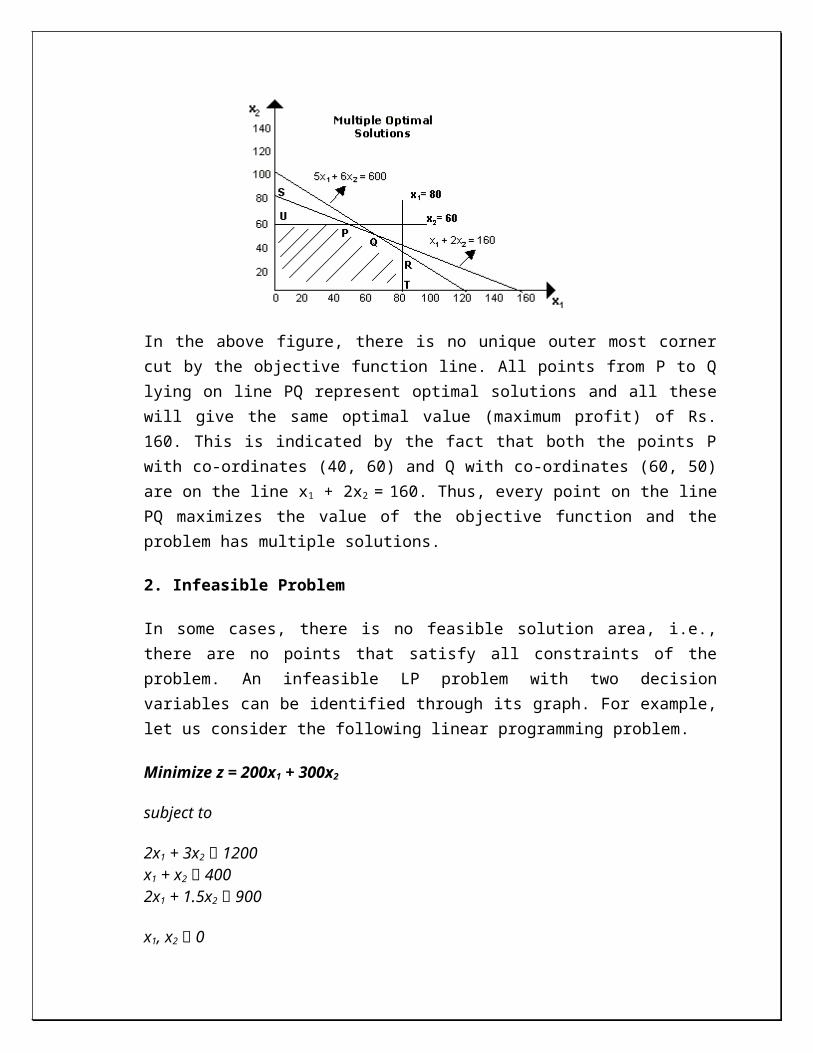
1. Multiple Optimal Solutions

The linear programming problems discussed in the previous section possessed unique solutions. This was because the optimal value occurred at one of the extreme points (corner points). But situations may arise, when the optimal solution obtained is not unique. This case may arise when the line representing the objective function is parallel to one of the lines bounding the feasible region. The presence of multiple solutions is

Maximize z = x1 + 2x2

subject to

x1 80x2 605x1 + 6x2 600x1 + 2x2 160

x1, x2 0.

In the above figure, there is no unique outer most corner cut by the objective function line. All points from P to Q lying on line PQ represent optimal solutions and all these will give the same optimal value (maximum profit) of Rs. 160. This is indicated by the fact that both the points P with co-ordinates (40, 60) and Q with co-ordinates (60, 50) are on

the line x1 + 2x2 = 160. Thus, every point on the line PQ maximizes the value of the objective function and the problem has multiple solutions.

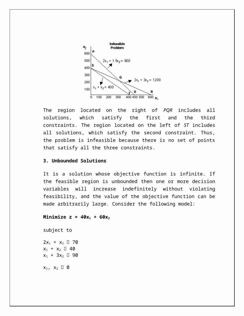
2. Infeasible Problem

In some cases, there is no feasible solution area, i.e., there are no points that satisfy all constraints of the problem. An infeasible LP problem with two decision variables can be identified through its graph. For example, let us consider the following linear programming problem.

Minimize z = 200x1 + 300x2

subject to

2x1 + 3x2 1200x1 + x2 4002x1 + 1.5x2 900

x1, x2 0

The region located on the right of PQR includes all solutions, which satisfy the first and the third constraints. The region located on the left of ST includes all solutions, which satisfy the second constraint. Thus, the problem is infeasible because there is no set of points that satisfy all the three constraints.

3. Unbounded Solutions

It is a solution whose objective function is infinite. If the feasible region is unbounded then one or more decision variables will increase indefinitely without violating

feasibility, and the value of the objective function can be made arbitrarily large. Consider the following model:

Minimize z = 40x1 + 60x2

subject to

2x1 + x2 70x1 + x2 40x1 + 3x2 90

x1, x2 0

The point (x1, x2) must be somewhere in the solution space as shown in the figure by shaded portion.

The three extreme points (corner points) in the finite plane are:P = (90, 0); Q = (24, 22) and R = (0, 70)The values of the objective function at these extreme points are:Z(P) = 3600, Z(Q) = 2280 and Z(R) = 4200

In this case, no maximum of the objective function exists because the region has no boundary for increasing values of x1 and x2. Thus, it is not possible to maximize the objective function in this case and the solution is unbounded.

The assignment problem can be stated as a problem where different jobs are to be assigned to different machines on the basis of the cost of doing these jobs. The objective is to minimize the total cost of doing all the jobs on different machines

4. How would you deal with the Assignment problems, where a) the objective function is to be maximized? b) Some Assignments are prohibited?

The peculiarity of the assignment problem is only one job can be assigned to one machine i.e., it should be a one-to-one assignment

The cost data is given as a matrix where rows correspond to jobs and columns to machines and there are as many rows as the number of columns i.e. the number of jobs and number of Machines should be equal

This can be compared to demand equals supply condition in a balanced transportation problem. In the optimal solution there should be only one assignment in each row and columns of the given assignment table. one can observe various situations where assignment problem can existing., assignment of workers to jobs like assigning clerks to different counters in a bank or salesman to different areas for sales, different contracts to bidders.

Assignment becomes a problem because each job requires different skills and the capacity or efficiency of each person with respect to these jobs can be different. This gives rise to cost differences. If each person is able to do all jobs equally efficiently then all costs will be the same and each job can be assigned to any person.

When assignment is a problem it becomes a typical optimization problem it can therefore be compared to a transportation problem. The cost elements are given and is a square matrix and requirement at each destination is one and availability at each origin is also one.

In addition we have number of origins which equals the number of destinations hence the total demand equals total supply . There is only one assignment in each row and each column .However If we compare this to a transportation problem we find that a general transportation problem does not have the above mentioned limitations. These limitations are peculiar to assignment problem only.

The assignment problem is a special type of transportation problem, where the objective is to minimize the cost or time of completing a number of jobs by a number of persons. In other words, when the problem involves the allocation of n different facilities to n different tasks, it is often termed as an assignment problem. The model's primary usefulness is for planning. The assignment problem also encompasses an important sub-class of so-called shortest- (or longest-) route models. The assignment

model is useful in solving problems such as, assignment of machines to jobs, assignment of salesmen to sales territories, travelling salesman problem, etc.

It may be noted that with n facilities and n jobs, there are n! possible assignments. One way of finding an optimal assignment is to write all the n! possible arrangements, evaluate their total cost, and select the assignment with minimum cost. But, due to heavy computational burden this method is not suitable.

The objective of this section is to examine a computational method - an algorithm - for deriving solutions to the assignment problems. The following steps summarize the approach:

Steps

1. Identify the minimum element in each row and subtract it from every element of that row.

2. Identify the minimum element in each column and subtract it from every element of that column.

3. Make the assignments for the reduced matrix obtained from steps 1 and 2 in the following way:

i. For each row or column with a single zero value cell that has not be assigned or eliminated, box that zero value as an assigned cell.

ii. For every zero that becomes assigned, cross out (X) all other zeros in the same row and the same column.

iii. If for a row and a column, there are two or more zeros and one cannot be chosen by inspection, then you are at liberty to choose the cell arbitrarily for assignment.

iv. The above process may be continued until every zero cell is either assigned or crossed (X).

4. An optimal assignment is found, if the number of assigned cells equals the number of rows (and columns). In case you have chosen a zero cell arbitrarily, there may be alternate optimal solutions. If no optimal solution is found, go to step 5.

5. Draw the minimum number of vertical and horizontal lines necessary to cover all the zeros in the reduced matrix obtained from step 3 by adopting the following procedure:

i. Mark all the rows that do not have assignments.ii. Mark all the columns (not already marked) which have zeros in the

marked rows.

iii. Mark all the rows (not already marked) that have assignments in marked columns.

iv. Repeat steps 5 (i) to (iii) until no more rows or columns can be marked.v. Draw straight lines through all unmarked rows and marked columns.

6. Select the smallest element from all the uncovered elements. Subtract this smallest element from all the uncovered elements and add it to the elements, which lie at the intersection of two lines. Thus, we obtain another reduced matrix for fresh assignment.

7. Go to step 3 and repeat the procedure until you arrive at an optimal assignment.

There are different methods of solving an assignment problem:

1)Complete Enumeration Method: This method can be used in case of assignment. problems of small size. In such cases a complete enumeration and evaluation of all combinations of persons and jobs is possible.

One can select the optimal combination. We may also come across more than one optimal combination The number of combinations increases manifold as the size of the problem increases as the total number of possible combinations depends on the number of say, jobs and machines. Hence the use of enumeration method is not feasible in real world cases.

2) Simplex Method: The assignment problem can be formulated as a linear programming

problem and hence can be solved by using simplex method.However solving the problem using simplex method can be a tedious job.

3)Transportation Method: The assignment problem is comparable to a transportation problem hence transportation method of solution can be used to find optimum allocation. However the major problem is that allocation degenerate as the allocation is on basis one to one per person per person per job Hence we need a methodspecially designed to solve assignment problems.

4 )Hungarian Assignment Method (HAM): This method is based on the concept of opportunity cost and is more efficient in solving assignment problems. Method in case of a minimization problem.

As we are using the concept “opportunity this means that the cost of any opportunity that is lost while taking a particular decision or action is taken into account while making assignment. Given below are the steps involved to solve an assignment problem by using Hungarian method

Maximization method

In order to solve a maximization type problem we find the regret values instead of opportunity cost. the problem can be solved in two ways

The first method is by putting a negative sign before the values in the assignment matrix and then solves the sum as a minimization case using Hungarian methods as shown above.

Second method is to locate the largest value in the given matrix and subtract each element in the matrix from this value. Then one can solve this problem as a minimization case using the new modified matrix.

Hence there are mainly four methods to solve assignment problem but the most efficient and most widely used method is the Hungarian method

Prohibited Assignment

Sometimes it may happen that a particular resource (say a man or machine) cannot be assigned to perform a particular activity. In such cases, the cost of performing that particular activity by a particular resource is considered to be very high (written as M or ∞) so as to prohibit the entry of this pair of resource-activity into the final solution.

A usual assignment problem presumes that all jobs can be performed by all individuals there can be a free or unrestricted assignment of jobs and individuals. A prohibited assignment problem occurs when a machine may not be in, a position to perform a particular job as there be some technical difficulties in using a certain machine for a certain job. In such cases the assignment is constrained by given facts.

To solve this type problem of restriction on job assignment we will have to assign a very high cost M This ensures that restricted or impractical combination does not enter the optimal assignment plan which aims at minimization of total cost.

5. Simulation is an especially valuable tool in a situation where the mathematics needed to describe a system realistically is too complex to yield analytical solutions”. Elucidate.

Shortcomings of taking a simulation approach to solve an O.R. problem The range of application of simulation in business is extremely wide. Unlike other mathematical models, simulation can be easily understood by the users and thereby facilitates their active involvement. This makes the results more reliable and also ensures easy acceptance for implementation. The degree to which a simulation model can be made close to reality is dependent upon the ingenuity of the OR team who identifies the relevant variables as well as their behavior.

In case of other OR models, simulation helps the manager to strike a balance between opposing costs of providing facilities (usually meaning long term commitment of funds) and the opportunity and costs of not providing them.

The simulation approach is recognized as a powerful tool for management decision-making. Shortcoming of taking a simulation approach to solve O. R. problems are as follows;

1. It does not produce optimal results. Solutions are approximate, and it is some less than formal but ‘satisfactory’ approach to problem-solving only.

2. To be able to simulate systems, a fairly good knowledge of the parts or components of the system and their characteristics is required. The desire is to understand, explain and predict the dynamic behavior of the system or the sum total of these parts. Adequate knowledge of the system behavior.

3. Each simulation run like a single experiment conducted under a given set of conditions as defined by a set of values for the input solution. A number of simulation runs will be necessary and thus can be time consuming. As the number of variables increases in terms of input, the difficulty in finding the optimum values increases considerably.

4. Since simulation involves repetitions of the experiment, it is a time consuming task when manually done.

5. As a number of parameters, increase, the difficulty in finding the optimum values increases to a considerable extent.

6. Because of the simplicity in adoption of simulation process, one may develop to rely on this technique too often, although mathematical model is more suitable to the situation.

7. One should not ignore the cost associated with a simulation study for data collection, formation of the model. A good simulation model may be very expensive. Often it takes years to develop a usable corporate planning model.

8. The computer time as it is fairly significant.

9. A simulation application is based on the premise that the behavior pattern of relevant variables is known, and this very premise sometimes becomes questionable.

10. Not always can the probabilities be estimated with ease or desired reliability. The results of simulation should always be compared with solutions obtained by other methods wherever possible, and “tempered” with managerial judgment.

6. Describe Gomorys method of solving an all-integer programming problem.

An integer programming problem can be described as follows:Determine the value of unknowns X1, X2, …, XnSo as to optimize z = C1X1 + C2X2 + … CnXn

Subject to the constraintsai1 X1 + ai2 X2 + … + ain Xn = bi, i = 1,2, …, mand xj ≥ 0 j = 1, 2, …, nwhere xj being an integral value for j = 1, 2, …, k ≤ n.

If all the variables are constrained to take only integral value i.e. k = n, it is called an all (or pure) integer programming problem. In case only some of the variables are restricted to take integral value of rest (n – k) variables are free to take any one negative values, then the problem is known as mixed integer programming problem.

Gomory’s All – IPP Method:

An optimum solution to an I. P. P. is first obtained by using simplex method ignoring the restriction of integral values. In the optimum solution if all the variables have integer values, the current solution will be the desired optimum integer solution. Otherwise the given IPP is modified by inserting a new constraint called Gomory’s or secondary constraint which represents necessary condition for integrability and eliminates some non integer solution without losing any integral solution.

After adding the secondary constraint, the problem is then solved by dual simplex method to get an optimum integral solution. If all the values of the variables in this solution are integers, an optimum inter-solution is obtained, otherwise another new constrained is added to the modified L P P and the procedure is repeated.

An optimum integer solution will be reached eventually after introducing enough new constraints to eliminate all the superior non integer solutions. The construction of additional constraints, called secondary or Gomory’s constraints is so very important that it needs special attention.