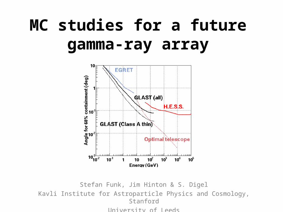
MC studies for a future gamma-ray array

Stefan Funk, Jim Hinton & S. Digel

Kavli Institute for Astroparticle Physics and Cosmology, Stanford

University of Leeds

• Part 1: Angular resolution MC-studies

• Part 2: Toy MC for fast exploration of phase space

• Part 3: The high-energy part of the array

• Part 4: Simulated Survey

Outline

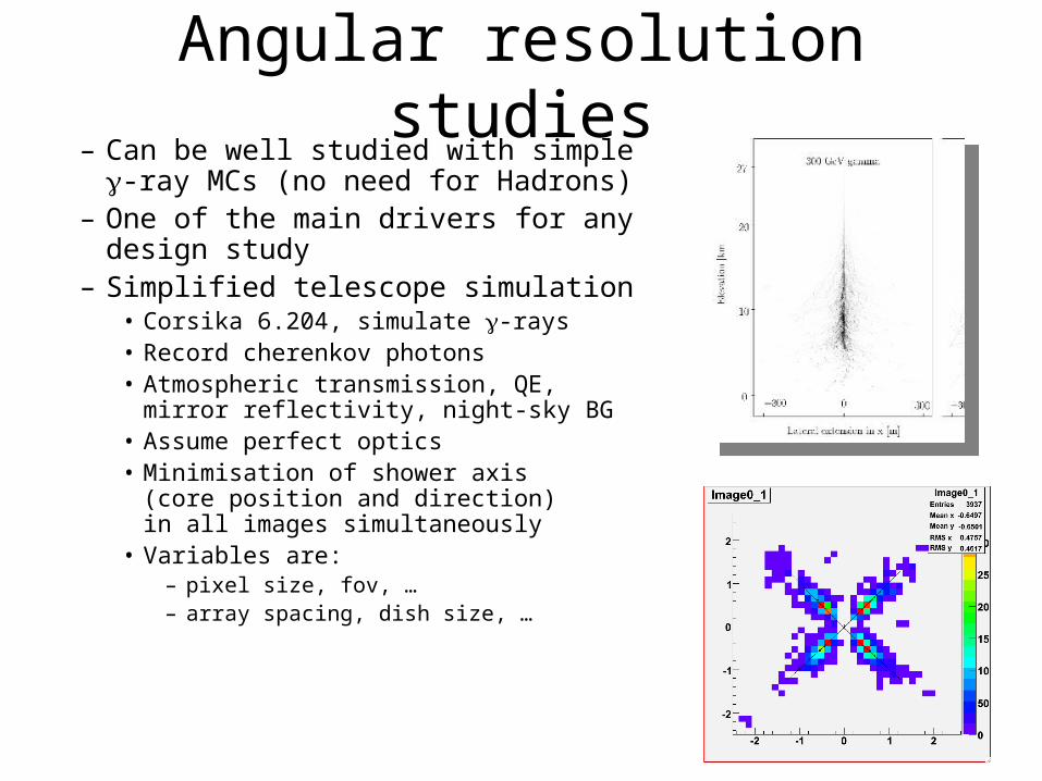
Angular resolution studies– Can be well studied with simple -ray

MCs (no need for Hadrons)– One of the main drivers for any design

study– Simplified telescope simulation

• Corsika 6.204, simulate -rays• Record cherenkov photons• Atmospheric transmission, QE,

mirror reflectivity, night-sky BG• Assume perfect optics• Minimisation of shower axis

(core position and direction) in all images simultaneously

• Variables are:– pixel size, fov, …– array spacing, dish size, …

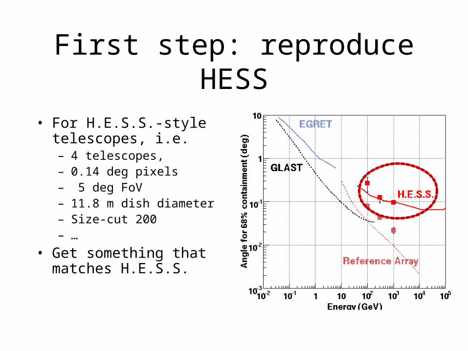
First step: reproduce HESS

• For H.E.S.S.-style telescopes, i.e. – 4 telescopes, – 0.14 deg pixels– 5 deg FoV– 11.8 m dish diameter– Size-cut 200– …

• Get something that matches H.E.S.S.

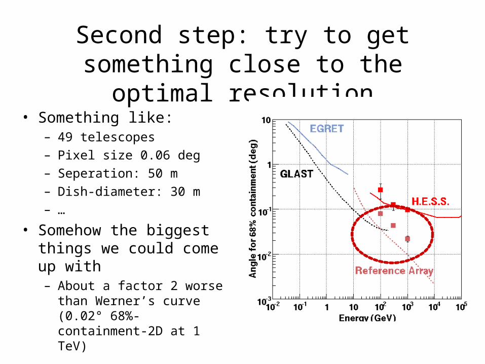
Second step: try to get something close to the optimal resolution

• Something like:– 49 telescopes– Pixel size 0.06 deg– Seperation: 50 m– Dish-diameter: 30 m– …

• Somehow the biggest things we could come up with– About a factor 2 worse than

Werner’s curve (0.02° 68%-containment-2D at 1 TeV)

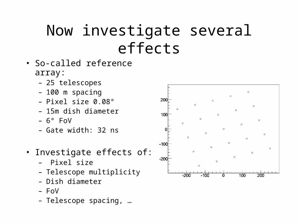
Now investigate several effects

• So-called reference array:– 25 telescopes– 100 m spacing– Pixel size 0.08°– 15m dish diameter– 6° FoV– Gate width: 32 ns

• Investigate effects of:– Pixel size– Telescope multiplicity– Dish diameter– FoV– Telescope spacing, …

Angular resolution vs pixelsize

• For reference array• Keep the FoV constant (at 6º)

and change the pixel size– Might be unrealistic (just

increases the number of pixels as pixel size decreases)

• Therefore try with fixed number of pixels (36x36) and adjust the field of view as the pixel size changes …– Also no strong dependence on pixel size

(different with different reconstruction algorithm?)

– … and FoV only matters if very small (1.44º for pix size 0.04º)

Angular resolution vs multiplicity• Started with array of

49 telescopes (distance: 100 m)– randomly kept 9, 16,

25, 36, 49 telescopes– Angular resolution vs

average multiplicity

• No strong dependence on any of the other tested parameters … (FoV, mirror size, …)

Use these finding to parametrise the curves …

• Explore the dependence of– angular resolution– hadron rejection power

• … on key factors such as:– Telescope multiplicity– Average size (in p.e.) of images– the impact distance range of the

measurements– the pixel size

(All as a function of energy)

• Critical inputs to the Toy MC as discussed in the next slides …

68 0.02 (E / TeV)0.62 ( (0.09/Ntels)2 + (0.17/<image_size>1/2)2 )1/2

degrees

Mostly by J. Hinton

QuickTime™ and a decompressor

are needed to see this picture.

… and then use them as input for the toy MC

• Driven by the need to explore the (rather large) phase-space– Full MC takes a LONG time to assess one

configuration – how can we optimise the array?– Using an approximate Toy MC we can explore

(orders of magnitude) more of the phase space and find plausible candidate array layouts to simulate in detail

– BUT:• This is only useful if the Toy MC has realistic

inputs and has real predictive power

Mostly by J. Hinton

Inputs to the Toy model

• Only Vertical showers• Cherenkov Light Density (r, E) [ LDF ]• Displacement of image with impact distance• Fluctuations: Xmax, E, and Poisson in image

Effective Area Curves Gamma-ray rate (E)

• Background rate?– Electron and Proton spectra– Angular resolution parameterisation

• Versus <size> and <Ntels>– BG rejection eff. parameterisation

• Versus <size> and <Ntels> Sensitivity (E)

phot

oele

ctro

ns/m

2 /G

eV

Impact distance (m)

e.g. 200 GeV

Taken from de la Calle & Perez (2006)

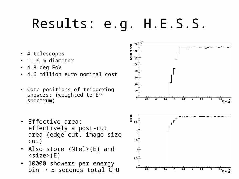
Results: e.g. H.E.S.S.

• 4 telescopes• 11.6 m diameter• 4.8 deg FoV• 4.6 million euro nominal cost

• Core positions of triggering showers: (weighted to E-2 spectrum)

• Effective area: effectively a post-cut area (edge cut, image size cut)

• Also store <Ntel>(E) and <size>(E)

• 10000 showers per energy bin 5 seconds total CPU

Resulting H.E.S.S. sensitivity

Integral: E*Fmin(>E)

Differential: half decades

full HE.S.S. MC

BG limited

>10 s

Resulting AGIS/CTA sensitivity

• Bernloehr-style array (85 + 4 telescopes)

• Can be reproduced quite well with the toy MC …

full MC (KB)

HESS

Toy

Optimisation for a grid …• Cost is fixed ($ 100M)• Number of tels varies• Free parameters

– FoV– Telescope separation– Dish size

• Pixel size kept fixed for the moment– Key input is missing

(effect on hadron rejection of pixel size)

• Grid search in 2-D planes within 3-D space …

Telescope Separation (m)

Pho

tons

cm

-2 s

-1 (

>1

TeV

)

180 60 m

• For a Crab-like spectrum and point-like source

Example: HESS type array, optimise separation.

280 m, 6.5 deg

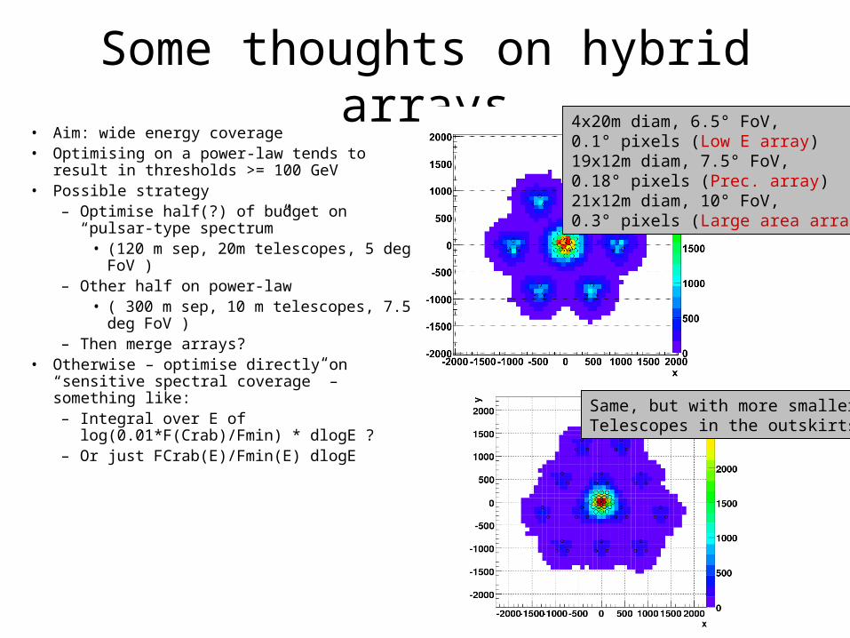
Some thoughts on hybrid arrays• Aim: wide energy coverage• Optimising on a power-law tends to

result in thresholds >= 100 GeV• Possible strategy

– Optimise half(?) of budget on “pulsar-type spectrum”

• (120 m sep, 20m telescopes, 5 deg FoV )

– Other half on power-law• ( 300 m sep, 10 m telescopes, 7.5 deg

FoV )– Then merge arrays?

• Otherwise – optimise directly on “sensitive spectral coverage” – something like:– Integral over E of log(0.01*F(Crab)/Fmin) *

dlogE ?– Or just FCrab(E)/Fmin(E) dlogE

4x20m diam, 6.5° FoV,0.1° pixels (Low E array)19x12m diam, 7.5° FoV,0.18° pixels (Prec. array)21x12m diam, 10° FoV,0.3° pixels (Large area array)

Same, but with more smallerTelescopes in the outskirts

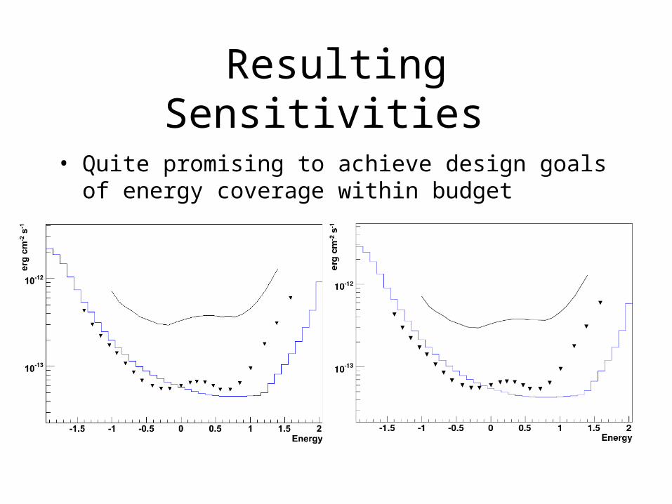
Resulting Sensitivities

• Quite promising to achieve design goals of energy coverage within budget

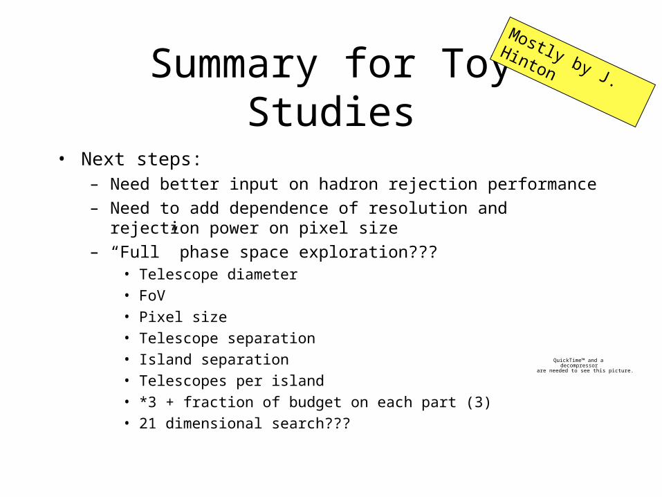
Summary for Toy Studies

• Next steps:– Need better input on hadron rejection performance

– Need to add dependence of resolution and rejection power on pixel size

– “Full” phase space exploration???• Telescope diameter• FoV• Pixel size• Telescope separation• Island separation• Telescopes per island• *3 + fraction of budget on each part (3)• 21 dimensional search???

QuickTime™ and a decompressor

are needed to see this picture.

Mostly by J. Hinton

Part 3: The high-energy part of the array

• How would one design an optimal array for the highest energies?– In terms of angular resolution and

optimal coverage for 20-100 TeV region– Requirements:

• Small dishes, large FoV, largish pixels … very relaxed requirements (lots of light!)

• How large? Will answer this with our simulations …

– Could easily surpass existing arrays where we are limited by the small FoV …

– … more to come on this rather soon!

QuickTime™ and a decompressor

are needed to see this picture.

QuickTime™ and a decompressor

are needed to see this picture.

Part 4: The simulated survey– Using H.E.S.S. backgrounds and a

source population model to predict the outcome of a Galactic plane survey with a future instrument

• E.g.: factor 10 better sensitivity– Factor 10 larger area

– Factor 2 better PSF

– Factor 2 better background rejection

HESS : ~500 hours

Together with J.

Hinton and S. Digel

The ‘Galactic plane with a future TeV instrument

– Background:• Take H.E.S.S. survey data• Replace data with photons randomly

sampled from the acceptance function (number of gamma-ray-like events versus camera offset - excluding source regions) taking into account zenith-dependence

• This gives a “source-free” simulation of the HESS survey

– Includes realistic exposure times and exactly the same analysis scheme as for the ‘real’ HESS survey

‘HESS - no sources’ : ~500 hours

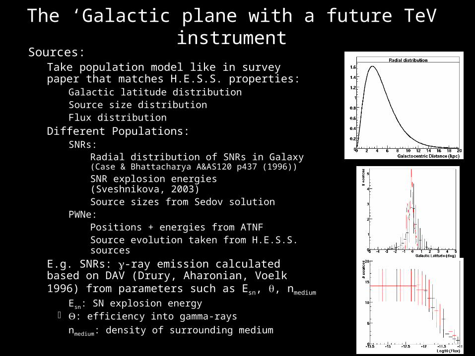
The ‘Galactic plane with a future TeV instrument– Sources:

• Take population model like in survey paper that matches H.E.S.S. properties:

– Galactic latitude distribution– Source size distribution– Flux distribution

• Different Populations:– SNRs:

» Radial distribution of SNRs in Galaxy (Case & Bhattacharya A&AS120 p437 (1996))

» SNR explosion energies(Sveshnikova, 2003)

» Source sizes from Sedov solution– PWNe:

» Positions + energies from ATNF» Source evolution taken from H.E.S.S. sources

• E.g. SNRs: -ray emission calculated based on DAV (Drury, Aharonian, Voelk 1996) from parameters such as Esn, , nmedium

– Esn: SN explosion energy : efficiency into gamma-rays– nmedium: density of surrounding medium

Matching H.E.S.S.

– Need smallish scale height (30pc) to match narrow H.E.S.S. distribution

• Rather normal efficiency into -rays: 9%• About 10 SNRs per century• … yields very good agreement (putting in

H.E.S.S. source parameters, not source model)

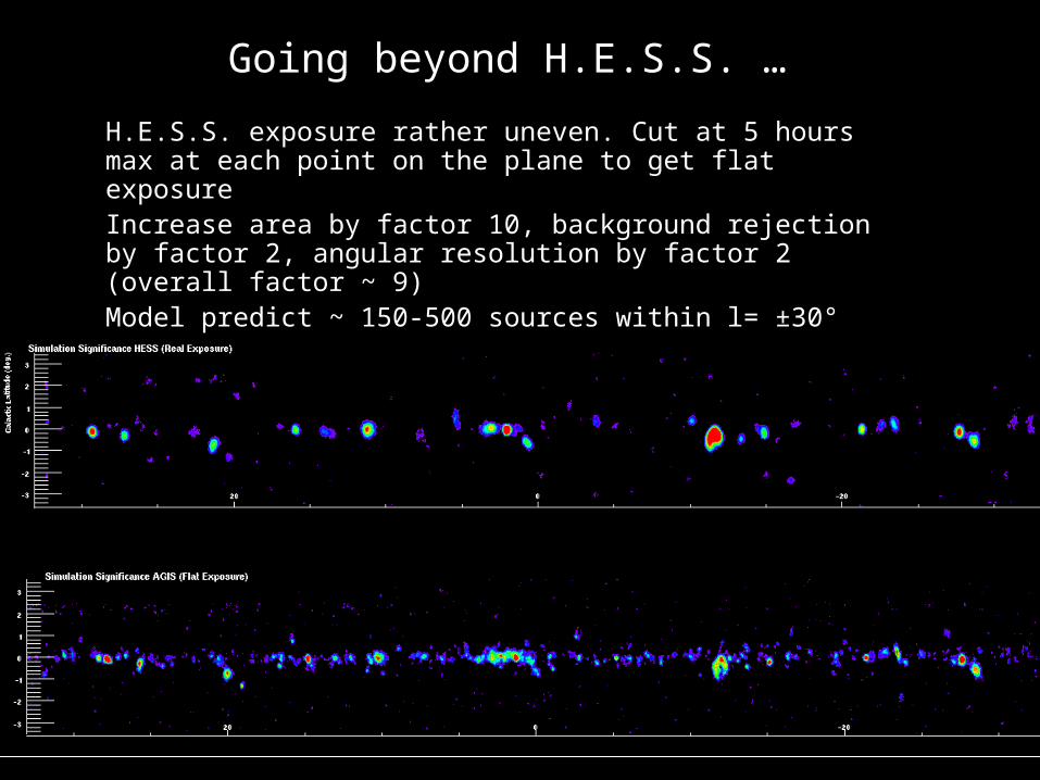
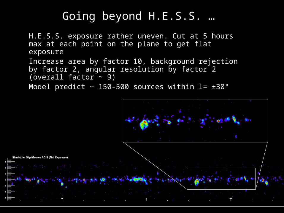
Going beyond H.E.S.S. …

– H.E.S.S. exposure rather uneven. Cut at 5 hours max at each point on the plane to get flat exposure

– Increase area by factor 10, background rejection by factor 2, angular resolution by factor 2 (overall factor ~ 9)

– Model predict ~ 150-500 sources within l= ±30°

Going beyond H.E.S.S. …

– H.E.S.S. exposure rather uneven. Cut at 5 hours max at each point on the plane to get flat exposure

– Increase area by factor 10, background rejection by factor 2, angular resolution by factor 2 (overall factor ~ 9)

– Model predict ~ 150-500 sources within l= ±30°

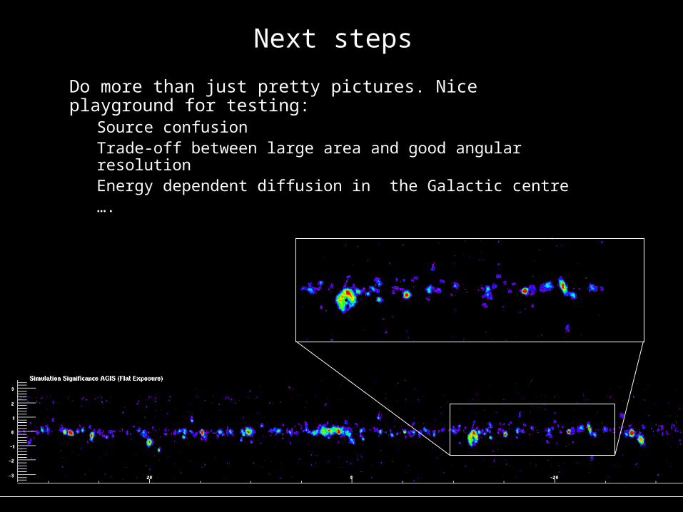
Next steps

– Do more than just pretty pictures. Nice playground for testing:• Source confusion• Trade-off between large area and good angular resolution• Energy dependent diffusion in the Galactic centre • ….

Summary

• Simple MC to determine main dependencies of angular resolution

• Combined with Toy MC to explore phase space

• Working on characterisation of high-energy array

• The simulated survey is a nice playground for testing physics questions