THE 18TH EUROPEAN CONFERENCE ON MACHINE LEARNINGAND

THE 11TH EUROPEAN CONFERENCE ON PRINCIPLES AND PRACTICEOF KNOWLEDGE DISCOVERY IN DATABASES

PROCEEDINGS OF THE

THIRD INTERNATIONAL

WORKSHOP ONMINING COMPLEX DATA

MCD 2007

September 17 and 21, 2007

Warsaw, Poland

Editors:Zbigniew W. RasUniversity of North Carolina at Charlotte, USADjamel ZighedUniversite Lyon II, FranceShusaku TsumotoShimane Medical University, Japan

Preface

Data mining and knowledge discovery, as stated in their early definition, can today beconsidered as stable fields with numerous efficient methods and studies that have beenproposed to extract knowledge from data. Nevertheless, the famous golden nugget isstill challenging. Actually, the context evolved since the first definition of the KDDprocess has been given and knowledge has now to be extracted from data getting moreand more complex.

In the framework of Data Mining, many software solutions were developed for theextraction of knowledge from tabular data (which are typically obtained from relationaldatabases). Methodological extensions were proposed to deal with data initially ob-tained from other sources, like in the context of natural language (text mining) andimage (image mining). KDD has thus evolved following a unimodal scheme instanti-ated according to the type of the underlying data (tabular data, text, images, etc), which,at the end, always leads to working on the classical double entry tabular format.

However, in a large number of application domains, this unimodal approach ap-pears to be too restrictive. Consider for instance a corpus of medical files. Each file cancontain tabular data such as results of biological analyzes, textual data coming fromclinical reports, image data such as radiographies, echograms, or electrocardiograms.In a decision making framework, treating each type of information separately has seri-ous drawbacks. It appears therefore more and more necessary to consider these differentdata simultaneously, thereby encompassing all their complexity.

Hence, a natural question arises: how could one combine information of differentnature and associate them with a same semantic unit, which is for instance the patient?On a methodological level, one could also wonder how to compare such complex unitsvia similarity measures. The classical approach consists in aggregating partial dissim-ilarities computed on components of the same type. However, this approach tends tomake superposed layers of information. It considers that the whole entity is the sumof its components. By analogy with the analysis of complex systems, it appears thatknowledge discovery in complex data can not simply consist of the concatenation ofthe partial information obtained from each part of the object. The aim would rather beto discover more global knowledge giving a meaning to the components and associatingthem with the semantic unit. This fundamental information cannot be extracted by thecurrently considered approaches and the available tools.

The new data mining strategies shall take into account the specificities of complexobjects (units with which are associated the complex data). These specificities are sum-marized hereafter:

Different kind. The data associated to an object are of different types. Besidesclassical numerical, categorical or symbolic descriptors, text, image or audio/video dataare often available.

Diversity of the sources. The data come from different sources. As shown in thecontext of medical files, the collected data can come from surveys filled in by doctors,textual reports, measures acquired from medical equipment, radiographies, echograms,etc.

Evolving and distributed. It often happens that the same object is described ac-cording to the same characteristics at different times or different places. For instance,a patient may often consult several doctors, each one of them producing specific infor-mation. These different data are associated with the same subject.

Linked to expert knowledge. Intelligent data mining should also take into accountexternal information, also called expert knowledge, which could be taken into accountby means of ontology. In the framework of oncology for instance, the expert knowledgeis organized under the form of decision trees and is made available under the form of“best practice guides” called Standard Option Recommendations (SOR).

Dimensionality of the data. The association of different data sources at differentmoments multiplies the points of view and therefore the number of potential descriptors.The resulting high dimensionality is the cause of both algorithmic and methodologicaldifficulties.

The difficulty of Knowledge Discovery in complex data lies in all these specificities.

We wish to express our gratitude to all members of the Program Committee andthe Organizing Committee. Hakim Hacid (Chair of the Organizing Committee) did aterrific job of putting together and maintaining the home page for the workshop as wellas helping us to prepare the workshop proceedings.

Zbigniew W. RasDjamel ZighedShusaku Tsumoto

MCD 2007 Workshop Committee

Workshop Chairs:Zbigniew W. Ras (Univ. of North Carolina, Charlotte)Djamel Zighed (Univ. Lyon II, France)Shusaku Tsumoto (Shimane Medical Univ., Japan)

Organizing Committee:Hakim Hacid (Univ. Lyon II, France)(Chair)Rory Lewis (Univ. of North Carolina, Charlotte)Xin Zhang (Univ. of North Carolina, Charlotte)

Program Committee:Aijun An (York Univ., Canada)Elisa Bertino (Purdue Univ., USA)Ivan Bratko (Univ. of Ljubljana, Slovenia)Michelangelo Ceci (Univ. Bari, Italy)Juan-Carlos Cubero (Univ of Granada, Spain)Tapio Elomaa (Tampere Univ. of Technology, Finland)Floriana Esposito (Univ. Bari, Italy)Mirsad Hadzikadic (UNC-Charlotte, USA)Howard Hamilton (Univ. Regina, Canada)Shoji Hirano (Shimane Univ., Japan)Mieczyslaw Klopotek (ICS PAS, Poland)Bozena Kostek (Technical Univ. of Gdansk, Poland)Nada Lavrac (Jozef Stefan Institute, Slovenia)Tsau Young Lin (San Jose State Univ., USA)Jiming Liu (Univ. of Windsor, Canada)Hiroshi Motoda (AFOSR/AOARD & Osaka Univ., Japan)James Peters (Univ. of Manitoba, Canada)Jean-Marc Petit (LIRIS, INSA Lyon, France)Vijay Raghavan (Univ. of Louisiana, USA)Jan Rauch (Univ. of Economics, Prague, Czech Republic)Henryk Rybinski (Warsaw Univ. of Technology, Poland)Dominik Slezak (Infobright, Canada)Roman Slowinski (Poznan Univ. of Technology, Poland)Jurek Stefanowski (Poznan Univ. of Technology, Poland)Juan Vargas (Microsoft, USA)Alicja Wieczorkowska (PJIIT, Poland)Xindong Wu (Univ. of Vermont, USA)Yiyu Yao (Univ. Regina, Canada)Ning Zhong (Maebashi Inst. of Tech., Japan)

Table of Contents

Using Text Mining and Link Analysis for Software Mining . . . . . . . . . . . . . . . . . . 1Miha Grcar, Marko Grobelnik, and Dunja Mladenic

Generalization-based Similarity for Conceptual Clustering . . . . . . . . . . . . . . . . . . . 13S. Ferilli, T.M.A. Basile, N. Di Mauro, M. Biba, and F. Esposito

Finding Composite Episodes . . . . . . . . . . . . . . . . . . . . . . . . . . . . . . . . . . . . . . . . . . 25Ronnie Bathoorn and Arno Siebes

Using Secondary Knowledge to Support Decision Tree Classification of Retro-spective Clinical Data . . . . . . . . . . . . . . . . . . . . . . . . . . . . . . . . . . . . . . . . . . . . . . . . 37

Dympna O’Sullivan, William Elazmeh, Szymon Wilk, Ken Farion, Stan Matwin,Wojtek Michalowski, Morvarid Sehatkar

Evaluating a Trading Rule Mining Method based on Temporal Pattern Extraction . 49Hidenao Abe, Satoru Hirabayashi, Miho Ohsaki, Takahira Yamaguchi

Discriminant Feature Analysis for Music Timbre Recognition . . . . . . . . . . . . . . . . 59Xin Zhang, Zbigniew W. Ras

Discovery of Frequent Graph Patterns that Consist of the Vertices with the Com-plex Structures . . . . . . . . . . . . . . . . . . . . . . . . . . . . . . . . . . . . . . . . . . . . . . . . . . . . . 71

Tsubasa Yamamoto, Tomonobu Ozaki, Takenao Okawa

Learning to Order Basic Components of Structured Complex Objects . . . . . . . . . . 83Donato Malerba, Michelangelo Ceci

ARoGS: Action Rules Discovery based on Grabbing Strategy and LERS . . . . . . . 95Zbigniew W. Ras, Elzbieta Wyrzykowska

Discovering Word Meanings Based on Frequent Termsets . . . . . . . . . . . . . . . . . . . 106Henryk Rybinski, Marzena Kryszkiewicz, Grzegorz Protaziuk, Aleksandra Kon-tkiewicz, Katarzyna Marcinkowska, Alexandre Delteil

Feature Selection: Near Set Approach . . . . . . . . . . . . . . . . . . . . . . . . . . . . . . . . . . . 116James F. Peters, Sheela Ramanna

Contextual Adaptive Clustering with Personalization . . . . . . . . . . . . . . . . . . . . . . . 128Krzysztof Ciesielski, Mieczysław A. Kłopotek, Sławomir Wierzchon

Unsupervised Grouping of Trajectory Data on Laboratory Examinations for Find-ing Exacerbating Cases in Chronic Diseases . . . . . . . . . . . . . . . . . . . . . . . . . . . . . . 139

Shoji Hirano, Shusaku Tsumoto

Improving Boosting by Exploiting Former Assumptions . . . . . . . . . . . . . . . . . . . . . 151Emna Bahri, Nicolas Nicoloyannis, Mondher Maddouri

Ordinal Classification with Decision Rules . . . . . . . . . . . . . . . . . . . . . . . . . . . . . . . 163Krzysztof Dembczynski, Wojciech Kotłowski, Roman Słowinski

Quality of Musical Instrument Sound Identification for Various Levels of Ac-companying Sounds . . . . . . . . . . . . . . . . . . . . . . . . . . . . . . . . . . . . . . . . . . . . . . . . . 175

Alicja Wieczorkowska, Elzbieta Kolczynska

Estimating Semantic Distance Between Concepts for Semantic HeterogeneousInformation Retrieval . . . . . . . . . . . . . . . . . . . . . . . . . . . . . . . . . . . . . . . . . . . . . . . . 185

Ahmad El Sayed, Hakim Hacid, Djamel Zighed

Clustering Individuals in Ontologies: a Distance-based Evolutionary Approach . . 197Nicola Fanizzi, Claudia d’Amato, Floriana Esposito

Data Mining of Multi-categorized Data . . . . . . . . . . . . . . . . . . . . . . . . . . . . . . . . . . 209Akinori Abe, Norihiro Hagita, Michiko Furutani, Yoshiyuki Furutani,and Rumiko Matsuoka

POM Centric Multiaspect Data Analysis for Investigating Human Problem Solv-ing Function . . . . . . . . . . . . . . . . . . . . . . . . . . . . . . . . . . . . . . . . . . . . . . . . . . . . . . . 221

Shinichi Motomura, Akinori Hara, Ning Zhong, Shengfu Lu

Author Index . . . . . . . . . . . . . . . . . . . . . . . . . . . . . . . . . . . . . . . . . . . . . . . . . . . . 233

Using Text Mining and Link Analysis for Software Mining

Miha Grcar1, Marko Grobelnik1, Dunja Mladenic1

1 Jozef Stefan Institute, Dept. of Knowledge Technologies, Jamova 39, 1000 Ljubljana, Slovenia

{miha.grcar, marko.grobelnik, dunja.mladenic}@ijs.si

Abstract. Many data mining techniques are these days in use for ontology learning – text mining, Web mining, graph mining, link analysis, relational data mining, and so on. In the current state-of-the-art bundle there is a lack of “software mining” techniques. This term denotes the process of extracting knowledge out of source code. In this paper we approach the software mining task with a combination of text mining and link analysis techniques. We discuss how each instance (i.e. a programming construct such as a class or a method) can be converted into a feature vector that combines the information about how the instance is interlinked with other instances, and the information about its (textual) content. The so-obtained feature vectors serve as the basis for the construction of the domain ontology with OntoGen, an existing system for semi-automatic data-driven ontology construction.

Keywords: software mining, text mining, link analysis, graph and network theory, feature vectors, ontologies, OntoGen, machine learning

1 Introduction and Motivation

Many data mining (i.e. knowledge discovery) techniques are these days in use for ontology learning – text mining, Web mining, graph mining, network analysis, link analysis, relation data mining, stream mining, and so on [6]. In the current state-of-the-art bundle mining of software code and the associated documentations is not explicitly addressed. With the growing amounts of software, especially open-source software libraries, we argue that mining such data is worth considering as a new methodology. Thus we introduce the term “software mining” to refer to such methodology. The term denotes the process of extracting knowledge (i.e. useful information) out of data sources that typically accompany an open-source software library.

The motivation for software mining comes from the fact that the discovery of reusable software artifacts is just as important as the discovery of documents and multimedia contents. According to the recent Semantic Web trends, contents need to be semantically annotated with concepts from the domain ontology in order to be discoverable by intelligent agents. Because the legacy content repositories are relatively large, cheaper semi-automatic means for semantic annotation and domain

1

ontology construction are preferred to the expensive manual labor. Furthermore, when dealing with software artifacts it is possible to go beyond discovery and also support other user tasks such as composition, orchestration, and execution. The need for ontology-based systems has yield several research and development projects supported by EU that deal with this issue. One of these projects is TAO (http://www.tao-project.eu) which stands for Transitioning Applications to Ontologies. In this paper we present work in the context of software mining for the domain ontology construction. We illustrate the proposed approach on the software mining case study based on GATE [3], an open-source software library for natural-language processing written in Java programming language.

We interpret “software mining” as being a combination of methods for structure mining and for content mining. To be more specific, we approach the software mining task with the techniques used for text mining and link analysis. The GATE case study serves as a perfect example in this perspective. On concrete examples we discuss how each instance (i.e. a programming construct such as a class or a method) can be represented as a feature vector that combines the information about how the instance is interlinked with other instances, and the information about its (textual) content. The so-obtained feature vectors serve as the basis for the construction of the domain ontology with OntoGen [4], a system for semi-automatic, data-driven ontology construction, or by using traditional machine learning algorithms such as clustering, classification, regression, or active learning.

2 Related Work

When studying the literature we did not limit ourselves to ontology learning in the context of software artifacts – the reason for this is in the fact that the more general techniques also have the potential to be adapted for software mining.

Several knowledge discovery (mostly machine learning) techniques have been employed for ontology learning in the past. Unsupervised learning, classification, active learning, and feature space visualization form the core of OntoGen [4]. OntoGen employs text mining techniques to facilitate the construction of an ontology out of a set of textual documents. Text mining seems to be a popular approach to ontology learning because there are many textual sources available (one of the largest is the Web). Furthermore, text mining techniques are shown to produce relatively good results. In [8], the authors provide a lot of insight into the ontology learning in the context of the Text-To-Onto ontology learning architecture. The authors employ a multi-strategy learning approach and result combination (i.e. they combine outputs of several different algorithms) to produce a coherent ontology definition. In this same work a comprehensive survey of ontology learning approaches is presented.

Marta Sabou’s thesis [13] provides valuable insights into ontology learning for Web Services. It summarizes ontology learning approaches, ontology learning tools, acquisition of software semantics, and describes – in detail – their framework for learning Web Service domain ontologies.

There are basically two approaches to building tools for software component discovery: the information retrieval approach and the knowledge-based approach. The

2

first approach is based on the natural language documentation of the software components. With this approach no interpretation of the documentation is made – the information is extracted via statistical analyses of the words distribution. On the other hand, the knowledge-based approach relies on pre-encoded, manually provided information (the information is provided by a domain expert). Knowledge-based systems can be “smarter” than IR systems but they suffer from the scalability issue (extending the repository is not “cheap”).

In [9], the authors present techniques for browsing amongst functionality related classes (rather than inheritance), and retrieving classes from object-oriented libraries. They chose the IR approach for which they believe is advantageous in terms of cost, scalability, and ease of posing queries. They extract information from the source code (a structured data source) and its associated documentation (an unstructured data source). First, the source code is parsed and the relations, such as derived-from or member-of, are extracted. They used a hierarchical clustering technique to form a browse hierarchy that reflected the degree of similarity between classes (the similarity is drawn from the class documentation rather than from the class structure). The similarity between two classes was inferred from the browse hierarchy with respect to the distance of the two classes from their common parent and the distance of their common parent from the root node.

In this paper we adopt some ideas from [9]. However, the purpose of our methodology is not to build browse hierarchies but rather to describe programming constructs with feature vectors that can be used for machine learning. In other words, the purpose of our methodology is to transform a source code repository into a feature space. The exploration of this feature space enables the domain experts to build a knowledge base in a “cheaper” semi-automatic interactive fashion.

3 Mining Content and Structure of Software Artifacts

In this section we present our approach and give an illustrative example of data preprocessing from documented source code using the GATE software library. In the context of the GATE case study the content is provided by the reference manual (textual descriptions of Java classes and methods), source code comments, programmer’s guide, annotator’s guide, user’s guide, forum, and so on. The structure is provided implicitly from these same data sources since a Java class or method is often referenced from the context of another Java class or method (e.g. a Java class name is mentioned in the comment of another Java class). Additional structure can be harvested from the source code (e.g. a Java class contains a member method that returns an instance of another Java class), code snippets, and usage logs (e.g. one Java class is often instantiated immediately after another). In this paper we limit ourselves to the source code which also represents the reference manual (the so called JavaDoc) since the reference manual is generated automatically out of the source code comments by a documentation tool.

A software-based domain ontology should provide two views on the corresponding software library: the view on the data structures and the view on the functionality [13]. In GATE, these two views are represented with Java classes and their member

3

methods – these are evident from the GATE source code. In our examples we limit ourselves to Java classes (i.e. we deal with the part of the domain ontology that covers the data structures of the system). This means that we will use the GATE Java classes as text mining instances (and also as graph vertices when dealing with the structure).

Let us first take a look at a typical GATE Java class. It contains the following bits of information relevant for the understanding of this example (see also Fig. 1): • Class comment. It should describe the purpose of the class. It is used by the

documentation tool to generate the reference manual (i.e. JavaDoc). It is mainly a source of textual data but also provides structure – two classes are interlinked if the name of one class is mentioned in the comment of the other class.

• Class name. Each class is given a name that uniquely identifies the class. The name is usually a composed word that captures the meaning of the class. It is mainly a source of textual data but also provides structure – two classes are interlinked if they share a common substring in their names.

• Field names and types. Each class contains a set of member fields. Each field has a name (which is unique within the scope of the class) and a type. The type of a field corresponds to a Java class. Field names provide textual data. Field types mainly provide structure – two classes are interlinked if one class contains a field that instantiates the other class.

• Field and method comments. Fields and methods can also be commented. The comment should explain the purpose of the field or method. These comments are a source of textual data. They can also provide structure in the same sense as class comments do.

• Method names and return types. Each class contains a set of member methods. Each method has a name, a set of parameters, and a return type. The return type of a method corresponds to a Java class. Each parameter has a name and a type which corresponds to a Java class. Methods can be treated similarly to fields with respect to taking their names and return types into account. Parameter types can be taken into account similarly to return types but there is a semantic difference between the two pieces of information. Parameter types denote classes that are “used/consumed” for processing while return types denote classes that are “produced” in the process.

• Information about inheritance and interface implementation. Each class inherits (fields and methods) from a base class. Furthermore, a class can implement one or more interfaces. An interface is merely a set of methods that need to be implemented in the derived class. The information about inheritance and interface implementation is a source of structural information.

3.1 Textual Content

Textual content is taken into account by assigning a textual document to each unit of the software code – in our illustrative example, to each GATE Java class. Suppose we focus on a particular arbitrary class – there are several ways to form the corresponding document.

4

Fig. 1. Relevant parts of a typical Java class.

It is important to include only those bits of text that are not misleading for the text mining algorithms. At this point the details of these text mining algorithms are pretty irrelevant provided that we can somehow evaluate the domain ontology that we build in the end.

Another thing to consider is how to include composed names of classes, fields, and methods into a document. We can insert each of these as: • a composed word (i.e. in its original form, e.g. “XmlDocumentFormat”), • separate words (i.e. by inserting spaces, e.g. “Xml Document Format”), or • combination of both (e.g. “XmlDocumentFormat Xml Document Format”).

The text-mining algorithms perceive two documents that have many words in common more similar that those that only share a few or no words. Breaking composed names into separate words therefore results in a greater similarity between documents that do not share full names but do share some parts of these names.

3.2 Determining the Structure

The basic units of the software code – in our case the Java classes – that we use as text-mining instances are interlinked in many ways. In this section we discuss how this structure which is often implicit can be determined from the source code.

As already mentioned, when dealing with the structure, we represent each class (i.e. each text mining instance) by a vertex in a graph. We can create several graphs – one for each type of associations between classes. This section describes several graphs that can be constructed out of object-oriented source code.

Comment Reference Graph. Every comment found in a class can reference another class by mentioning its name (for whatever the reason may be). In Fig. 1 we can see four such references, namely the class DocumentFormat references classes XmlDocumentFormat, RtfDocumentFormat, MpegDocumentFormat, and MimeType

5

(denoted with “Comment reference” in the figure). A section of the comment reference graph for the GATE case study is shown in Fig. 2. The vertices represent GATE Java classes found in the “gate” subfolder of the GATE source code repository (we limited ourselves to a subfolder merely to reduce the number of vertices for the purpose of the illustrative visualization). An arc that connects two vertices is directed from the source vertex towards the target vertex (these two vertices represent the source and the target class, respectively). The weight of an arc (at least 1) denotes the number of times the name of the target class is mentioned in the comments of the source class. The higher the weight, the stronger is the association between the two classes. In the figure, the thickness of an arc is proportional to its weight.

Name Similarity Graph. A class usually represents a data structure and a set of methods related to it. Not every class is a data structure – it can merely be a set of (static) methods. The name of a class is usually a noun denoting either the data structure that the class represents (e.g. Boolean, ArrayList) or a “category” of the methods contained in the class (e.g. System, Math). If the name is composed (e.g. ArrayList) it is reasonable to assume that each of the words bears a piece of information about the class (e.g. an ArrayList is some kind of List with the properties of an Array). Therefore it is also reasonable to say that two classes that have more words in common are more similar to each other than two classes that have fewer words in common. According to this intuition we can construct the name similarity

Fig. 2. A section of the GATE comment reference graph.

graph. This graph contains edges (i.e. undirected links) instead of arcs. Two vertices are linked when the two classes share at least one word. The strength of the link (i.e. the edge weight) can be computed by using the Jaccard similarity measure which is often used to measure the similarity of two sets of items (see http://en.wikipedia.org /wiki/Jaccard_index). The name similarity graph for the GATE case study is presented in Fig. 3. The vertices represent GATE Java classes found in the “gate” subfolder of the GATE source code repository. The Jaccard similarity measure was

6

used to weight the edges. Edges with weights lower than 0.6 and vertices of degree 0 were removed to simplify the visualization. In Fig. 3 we have removed class names and weight values to clearly show the structure. The evident clustering of vertices is the result of the Kamada-Kawai graph drawing algorithm [14] employed by Pajek [1] which was used to create graph drawings in this paper. The Kamada-Kawai algorithm positions vertices that are highly interlinked closer together.

Type Reference Graph. Field types and method return types are a valuable source of structural information. A field type or a method return type can correspond to a class in the scope of the study (i.e. a class that is also found in the source code repository under consideration) – hence an arc can be drawn from the class to which the field or the method belongs towards the class represented by the type.

Inheritance and Interface Implementation Graph. Last but not least, structure can also be determined from the information about inheritance and interface implementation. This is the most obvious structural information in an object-oriented source code and is often used to arrange classes into the browsing taxonomy. In this graph, an arc that connects two vertices is directed from the vertex that represents a base class (or an interface) towards the vertex that represents a class that inherits from the base class (or implements the interface). The weight of an arc is always 1.

Fig. 3. The GATE name similarity graph. The most common substrings in names are shown for the most evident clusters.

4 Transforming Content and Structure into Feature Vectors

Many data-mining algorithms work with feature vectors. This is true also for the algorithms employed by OntoGen and for the traditional machine learning algorithms such as clustering or classification. Therefore we need to convert the content (i.e.

Resource Persistence Controller

Annotation Corpus

Document WordNet

7

documents assigned to text-mining instances) and the structure (i.e. several graphs of interlinked vertices) into feature vectors. Potentially we also want to include other explicit features (e.g. in- and out-degree of a vertex).

4.1 Converting Content into Feature Vectors

To convert textual documents into feature vectors we resort to a well-known text mining approach. We first apply stemming1 to all the words in the document collection (i.e. we normalize words by stripping them of their suffixes, e.g. stripping → strip, suffixes → suffix). We then search for n-grams, i.e. sequences of consecutive words of length n that occur in the document collection more than a certain amount of times [11]. Discovered n-grams are perceived just as all the other (single) words. After that, we convert documents into their bag-of-words representations. To weight words (and n-grams), we use the TF-IDF weighting scheme ([6], Section 1.3.2).

4.2 Converting Structure into Feature Vectors

Let us repeat that the structure is represented in the form of several graphs in which vertices correspond to text-mining instances. If we consider a particular graph, the task is to describe each vertex in the graph with a feature vector.

For this purpose we adopt the technique presented in [10]. First, we convert arcs (i.e. directed links) into edges (i.e. undirected links)2. The edges adopt weights from the corresponding arcs. If two vertices are directly connected with more than one arc, the resulting edge weight is computed by summing, maximizing, minimizing, or averaging the arc weights (we propose summing the weights as the default option). Then we represent a graph on N vertices as a N×N sparse matrix. The matrix is constructed so that the Xth row gives information about vertex X and has nonzero components for the columns representing vertices from the neighborhood of vertex X. The neighborhood of a vertex is defined by its (restricted) domain. The domain of a vertex is the set of vertices that are path-connected to the vertex. More generally, a restricted domain of a vertex is a set of vertices that are path-connected to the vertex at a maximum distance of dmax steps [1]. The Xth row thus has a nonzero value in the Xth column (because vertex X has zero distance to itself) as well as nonzero values in all the other columns that represent vertices from the (restricted) domain of vertex X. A value in the matrix represents the importance of the vertex represented by the column for the description of the vertex represented by the row. In [10] the authors propose to compute the values as 1/2d, where d is the minimum path length between the two vertices (also termed the geodesic distance between two vertices) represented by the row and column.

1 We use the Porter stemmer for English (see http://de.wikipedia.org/wiki/Porter-Stemmer-

Algorithmus). 2 This is not a required step but it seems reasonable – a vertex is related to another vertex if

they are interconnected regardless of the direction. In other words, if vertex A references vertex B then vertex B is referenced by vertex A.

8

We also need to include edge weights into account. The easiest way is to use the weights merely for thresholding. This means that we set a threshold and remove all the edges that have weights below this threshold. After that we construct the matrix which now indirectly includes the information about the weights (at least to a certain extent).

The simple approach described above is based on more sophisticated approaches such as ScentTrails [12]. The idea is to metaphorically “waft” scent of a specific vertex in the direction of its out-links (links with higher weights conduct more scent than links with lower weights – the arc weights are thus taken into account explicitly). The scent is then iteratively spread throughout the graph. After that we can observe how much of the scent reached each of the other vertices. The amount of scent that reached a target vertex denotes the importance of the target vertex for the description of the source vertex.

The ScentTrails algorithm shows some similarities with the probabilistic framework: starting in a particular vertex and moving along the arcs we need to determine the probability of ending up in a particular target vertex within m steps. At each step we can select one of the available outgoing arcs with the probability proportional to the corresponding arc weight (assuming that the weight denotes the strength of the association between the two vertices). The equations for computing the probabilities are fairly easy to derive (see [7], Appendix C) but the time complexity of the computation is higher than that of ScentTrails and the first presented approach. The probabilistic framework is thus not feasible for large graphs.

4.3 Joining Different Representations into a Single Feature Vector

The next issue to solve is how to create a feature vector for a vertex that is present in several graphs at the same time (remember that the structure can be represented with more than one graph) and how to then also “append” the corresponding content feature vector. In general, this can be done in two different ways: • Horizontally. This means that feature vectors of the same vertex from different

graphs are first multiplied by factors αi (i = 1, ..., M) and then concatenated into a feature vector with M×N components (M being the number of graphs and N the number of vertices). The content feature vector is multiplied by αM+1 and simply appended to the resulting structure feature vector.

• Vertically. This means that feature vectors of the same vertex from different graphs are first multiplied by factors αi (i = 1, ..., M) and then summed together (component-wise) resulting in a feature vector with N components (N being the number of vertices). Note that the content feature vector cannot be summed together with the resulting structure feature vector since the features contained therein carry a different semantic meaning (not to mention that the two vectors are not of the same length). Therefore also in this case, the content feature vector is multiplied by αM+1 and appended to the resulting structure feature vector. Fig. 4 illustrates these two approaches. A factor αi (i = 1, ..., M) denotes the

importance of information provided by graph i, relative to the other graphs. Factor αM+1, on the other hand, denotes the importance of information provided by the content relative to the information provided by the structure. The easiest way to set

9

the factors is to either include the graph or the content (i.e. αi = 1), or to exclude it (i.e. αi = 0). In general these factors can be quite arbitrary. Pieces of information with lower factors contribute less to the outcomes of similarity measures used in clustering algorithms than those with higher factors. Furthermore, many classifiers are sensitive to this kind of weighting. For example, it has been shown in [2] that the SVM regression model is sensitive to how this kind of factors are set.

(a) Concatenating feature vectors.

(b) Summing feature vectors.

Fig. 4. The two different ways of joining several different representations of the same instance.

OntoGen includes a feature-space visualization tool called Document Atlas [5]. It is capable of visualizing high-dimensional feature space in two dimensions. The feature vectors are presented with two-dimensional points while the Euclidean distances between these points reflect cosine distances between feature vectors. It is not possible to perfectly preserve the distances from the high-dimensional space but even an approximation gives the user an idea of how the feature space looks like. Fig. 5 shows two such visualizations of the GATE case study data. In the left figure, only the class comments were taken into account (i.e. all the structural information was ignored and the documents assigned to the instances consisted merely of the corresponding class comments). In the right figure the information from the name similarity graph was added to the content information from the left figure. The content information was weighted twice higher than the structural information. dmax of the name similarity graph was set to 0.44.

The cluster marked in the left figure represents classes that provide functionality to consult WordNet (see http://wordnet.princeton.edu) to resolve synonymy3. The cluster containing this same functionality in the right figure is also marked. However, the cluster in the right figure contains more classes many of which were not commented thus were not assigned any content4. Contentless classes are stuck in the top left corner in the left figure because the feature-space visualization system did not know where to put them due to the lack of association with other classes. This missing

3 The marked cluster in the left figure contains classes such as Word, VerbFrame, and Synset. 4 The marked cluster in the right figure contains the same classes as the marked cluster in the

left figure but also some contentless classes such as WordImpl, VerbFrameImpl, (Mutable)LexKBSynset(Impl), SynsetImpl, WordNetViewer, and IndexFileWordNetImpl.

10

association was introduced with the information from the name similarity graph. From the figures it is also possible to see that clusters are better defined in the right figure (note the dense areas represented with light color).

Fig. 5. Two different semantic spaces obtained by two different weighting settings.

With these visualizations we merely want to demonstrate the difference in semantic spaces between two different settings. This is important because instances that are shown closer together are more likely to belong to the same cluster or category after applying clustering or classification. The weighting setting depends strongly on the context of the application of this methodology.

5 Conclusions

In this paper we presented a methodology for transforming a source code repository into a set of feature vectors, i.e. into a feature space. These feature vectors serve as the basis for the construction of the domain ontology with OntoGen, a system for semi-automatic data-driven ontology construction, or by using traditional machine learning algorithms such as clustering, classification, regression, or active learning. The presented methodology thus facilitates the transitioning of legacy software repositories into state-of-the-art ontology-based systems for discovery, composition, and potentially also execution of software artifacts.

This paper does not provide any evaluation of the presented methodology. Basically, the evaluation can be performed either by comparing the resulting ontologies with a golden-standard ontology (if such ontology exists) or, on the other hand, by employing them in practice. In the second scenario, we measure the efficiency of the users that are using these ontologies (directly or indirectly) in order to achieve certain goals. The aspects on the quality of the methods presented herein will be the focus of our future work.

We recently started developing an ontology-learning framework named LATINO which stands for Link-analysis and text-mining toolbox [7]. LATINO will be an open-source general purpose data mining platform providing (mostly) text mining, link analysis, machine learning, and data visualization capabilities.

Contentless classes

11

Acknowledgments. This work was supported by the Slovenian Research Agency and the IST Programme of the European Community under TAO Transitioning Applications to Ontologies (IST-4-026460-STP) and PASCAL Network of Excellence (IST-2002-506778).

References

1. Batagelj, V., Mrvar, A., de Nooy, W.: Exploratory Network Analysis with Pajek. Cambridge University Press (2004)

2. Brank, J., Leskovec, J.: The Download Estimation Task on KDD Cup 2003. In ACM SIGKDD Explorations Newsletter, volume 5, issue 2, 160–162, ACM Press, New York, USA (2003)

3. Cunningham, H., Maynard, D., Bontcheva, K., and Tablan, V.: GATE: A Framework and Graphical Development Environment for Robust NLP Tools and Applications. In Proceedings of the 40th Anniversary Meeting of the Association for Computational Linguistics ACL’02 (2002)

4. Fortuna, B, Grobelnik M., Mladenic D.: Semi-automatic Data-driven Ontology Construction System. In Proceedings of the 9th International Multi-conference Information Society IS-2006, Ljubljana, Slovenia (2006)

5. Fortuna, B., Mladenic, D., Grobelnik, M.: Visualization of Text Document Corpus. In Informatica 29, 497-502 (2005)

6. Grcar, M., Mladenic, D., Grobelnik, M., Bontcheva, K.: D2.1: Data Source Analysis and Method Selection. Project report IST-2004-026460 TAO, WP 2, D2.1 (2006)

7. Grcar, M., Mladenic, D., Grobelnik, M., Fortuna, B., Brank, J.: D2.2: Ontology Learning Implementation. Project report IST-2004-026460 TAO, WP 2, D2.2 (2006)

8. Maedche, A., Staab, S.: Discovering Conceptual Relations from Text. In Proc. of ECAI 2000, 321–325 (2001)

9. Helm, R., Maarek, Y.: Integrating Information Retrieval and Domain Specific Approaches for Browsing and Retrieval in Object-oriented Class Libraries. In Proceedings of Object-oriented Programming Systems, Languages, and Applications, 47–61, ACM Press, New York, USA (1991)

10. Mladenic, D, Grobelnik, M.: Visualizing Very Large Graphs Using Clustering Neighborhoods. In Local Pattern Detection, Dagstuhl Castle, Germany, April 12–16 (2004)

11. Mladenic, D., Grobelnik, M.: Word Sequences as Features in Text Learning. In Proceedings of the 17th Electrotechnical and Computer Science Conference ERK-98, Ljubljana, Slovenia (1998)

12. Olston, C., Chi, H. E.: ScentTrails: Integrating Browsing and Searching on the Web. In ACM Transactions on Computer-human Interaction TOCHI, volume 10, issue 3, 177–197, ACM Press, New York, USA (2003)

13. Sabou, M.: Building Web Service Ontologies. In SIKS Dissertation Series No. 2004-4, ISBN 90-9018400-7 (2006)

14. Kamada, T., Kawai, S.: An Algorithm for Drawing General Undirected Graphs. In Information Processing Letters 31, 7–15 (1989)

12

Generalization-based Similarityfor Conceptual Clustering

S. Ferilli, T.M.A. Basile, N. Di Mauro, M. Biba, and F. Esposito

Dipartimento di InformaticaUniversita di Bari

via E. Orabona, 4 - 70125 Bari - Italia{ferilli, basile, ndm, biba, esposito}@di.uniba.it

Abstract. Knowledge extraction represents an important issue thatconcerns the ability to identify valid, potentially useful and understand-able patterns from large data collections. Such a task becomes moredifficult if the domain of application cannot be represented by means ofan attribute-value representation. Thus, a more powerful representationlanguage, such as First-Order Logic, is necessary. Due to the complexityof handling First-Order Logic formulæ, where the presence of relationscauses various portions of one description to be possibly mapped in dif-ferent ways onto another description, few works presenting techniquesfor comparing descriptions are available in the literature for this kindof representations. Nevertheless, the ability to assess similarity betweenfirst-order descriptions has many applications, ranging from descriptionselection to flexible matching, from instance-based learning to clustering.

This paper tackles the case of Conceptual Clustering, where a new ap-proach to similarity evaluation, based on both syntactic and semanticfeatures, is exploited to support the task of grouping together similaritems according to their relational description. After presenting a frame-work for Horn Clauses (including criteria, a function and compositiontechniques for similarity assessment), classical clustering algorithms areexploited to carry out the grouping task. Experimental results on real-world datasets prove the effectiveness of the proposal.

1 Introduction

The large amount of information available nowadays makes more difficult thetask of extracting useful knowledge, i.e. valid, potentially useful and under-standable patterns, from data collections. Such a task becomes more difficultif the collection requires a more powerful representation language than simpleattribute-value vectors. First-order logic (FOL for short) is a powerful formal-ism, that is able to express relations between objects and hence can overcome thelimitations shown by propositional or attribute-value representations. However,the presence of relations causes various portions of one description to be possi-bly mapped in different ways onto another description, which poses problems ofcomputational effort when two descriptions have to be compared to each other.

13

Specifically, an important subclass of FOL refers to sets of Horn clauses, i.e.logical formulæ of the form l1∧· · ·∧ln ⇒ l0 where the li’s are atoms, usuallyrepresented in Prolog style as l0 :- l1, . . . , ln to be interpreted as “l0 (calledhead of the clause) is true, provided that l1 and ... and ln (called body of theclause) are all true”. Without loss of generality [16], we will deal with the caseof linked Datalog clauses.

The availability of techniques for the comparison between FOL (sub-)des-criptions could have many applications: helping a subsumption procedure toconverge quickly, guiding a generalization procedure by focussing on the compo-nents that are more similar and hence more likely to correspond to each other,implementing flexible matching, supporting instance-based classification tech-niques or conceptual clustering. Cluster analysis concerns the organization ofa collection of unlabeled patterns into groups (clusters) of homogeneous ele-ments based on their similarity. The similarity measure exploited to evaluatethe distance between elements is responsible for the effectiveness of the cluster-ing algorithms. Hence, the comparison techniques are generally defined in termsof a metric that must be carefully constructed if the clustering is to be relevant.In supervised clustering there is an associated output class value for each ele-ment and the efficacy of the metric exploited for the comparison of elements isevaluated according to the principle that elements belonging to the same classare clustered together as much as possible.

In the following sections, a similarity framework for first-order logic clauseswill be presented. Then, Section 5 will deal with related work, and Section 6will show how the proposed formula and criteria are able to effectively guide aclustering procedure for FOL descriptions. Lastly, Section 7 will conclude thepaper and outline future work directions.

2 Similarity Formula

Intuitively, the evaluation of similarity between two items i′ and i′′ might bebased both on the presence of common features, which should concur in a positiveway to the similarity evaluation, and on the features of each item that are notowned by the other, which should concur negatively to the whole similarity valueassigned to them [10]. Thus, plausible similarity parameters are:

n , the number of features owned by i′ but not by i′′ (residual of i′ wrt i′′);l , the number of features owned both by i′ and by i′′;m , the number of features owned by i′′ but not by i′ (residual of i′′ wrt i′).

A novel similarity function that expresses the degree of similarity between i′ andi′′ based on the above parameters, developed to overcome some limitations ofother functions in the literature (e.g., Tverski’s, Dice’s and Jaccard’s), is:

sf (i′, i′′) = sf(n, l,m) = 0.5l + 1

l + n + 2+ 0.5

l + 1l + m + 2

(1)

It takes values in ]0, 1[, to be interpreted as the degree of similarity betweenthe two items. A complete overlapping of the two items tends to the limit of 1

14

as long as the number of common features grows. The full-similarity value 1 isnever reached, and is reserved to the exact identification of items, i.e. i′ = i′′

(in the following, we assume i′ 6= i′′). Conversely, in case of no overlapping thefunction will tend to 0 as long as the number of non-shared features grows. Thisis consistent with the intuition that there is no limit to the number of differentfeatures owned by the two descriptions, which contribute to make them everdifferent. Since each of the two terms refers specifically to one of the two clausesunder comparison, a weight could be introduced to give different importance toeither of the two.

3 Similarity Criteria

The main contribution of this paper is in the exploitation of the formula invarious combinations that can assign a similarity degree to the different clauseconstituents. In FOL formulæ, terms represent specific objects; unary predicatesrepresent term properties and n-ary predicates express relationships. Hence, twolevels of similarity between first-order descriptions can be defined: the objectlevel, concerning similarities between terms in the descriptions, and the structureone, referring to how the nets of relationships in the descriptions overlap.

Example 1. Let us consider, as a running example throughout the paper, thefollowing toy clause (a real-world one would be too complex):

C : h(a) :- p(a, b), p(a, c), p(d, a), r(b, f), o(b, c), q(d, e), t(f, g),π(a), φ(a), σ(a), τ(a), σ(b), τ(b), φ(b), τ(d), ρ(d), π(f), φ(f), σ(f).

3.1 Object Similarity

Consider two clauses C ′ and C ′′. Call A′ = {a′1, . . . , a′n} the set of terms in C ′,and A′′ = {a′′1 , . . . , a′′m} the set of terms in C ′′. When comparing a pair of ob-jects (a′, a′′) ∈ A′ × A′′, two kinds of object features can be distinguished: theproperties they own as expressed by unary predicates (characteristic features),and the roles they play in n-ary predicates (relational features). More precisely,a role can be seen as a couple R = (predicate, position) (written compactly asR = predicate/arity.position), since different positions actually refer to differ-ent roles played by the objects. For instance, a characteristic feature could bemale(X), while relational features in a parent(X,Y) predicate are the ‘parent’role (parent/2.1) the ‘child’ role (parent/2.2).

Two corresponding similarity values can be associated to a′ and a′′: a char-acteristic similarity,

sfc(a′, a′′) = sf(nc, lc,mc)

based on the set P ′ of properties related to a′ and the set P ′′ of properties relatedto a′′, for the following parameters:

nc = |P ′ \ P ′′| number of properties owned by a′ in C ′ but not by a′′ in C ′′

(characteristic residual of a′ wrt a′′);

15

lc = |P ′ ∩ P ′′| number of common properties between a′ in C ′ and a′′ in C ′′;mc = |P ′′ \ P ′| number of properties owned by a′′ in C ′′ but not by a′ in C ′

(characteristic residual of a′′ wrt a′).

and a relational similarity,

sfr(a′, a′′) = sf(nr, lr,mr)

based on the multisets R′ and R′′ of roles played by a′ and a′′, respectively, forthe following parameters:

nr = |R′ \R′′| how many times a′ plays in C ′ role(s) that a′′ does not play inC ′′ (relational residual of a′ wrt a′′);

lr = |R′ ∩R′′| number of times that both a′ in C ′ and a′′ in C ′′ play the samerole(s);

mr = |R′′ \R′| how many times a′′ plays in C ′′ role(s) that a′ does not play inC ′ (relational residual of a′′ wrt a′).

Overall, we can define the object similarity between two terms as

sfo(a′, a′′) = sfc(a′, a′′) + sfr(a′, a′′)

Example 2. Referring to clause C, the set of properties of a is {π, φ, σ, τ}, for bit is {σ, τ} and for c it is {φ}. The multiset of roles of a is {p/2.1, p/2.1, p/2.2},for b it is {p/2.2, r/2.1, o/2.1} and for c it is {p/2.2, o/2.2}.

3.2 Structural Similarity

When checking for the structural similarity of two formulæ, many objects canbe involved, and hence their mutual relationships represent a constraint on howeach of them in the former formula can be mapped onto another in the latter. Thestructure of a formula is defined by the way in which n-ary atoms (predicatesapplied to a number of terms equal to their arity) are applied to the variousobjects to relate them. This is the most difficult part, since relations are specificto the first-order setting and are the cause of indeterminacy in mapping (partsof) a formula into (parts of) another one. In the following, we will call compatibletwo FOL (sub-)formulæ that can be mapped onto each other without yieldinginconsistent term associations (i.e., a term in one formula cannot correspond todifferent terms in the other formula).

Given an n-ary literal, we define its star as the multiset of n-ary predicatescorresponding to the literals linked to it by some common term (a predicate canappear in multiple instantiations among these literals). The star similarity be-tween two compatible n-ary literals l′ and l′′ having stars S′ and S′′, respectively,can be computed for the following parameters:

ns = |S′ \ S′′| how many more relations l′ has in C ′ than l′′ has in C ′′ (starresidual of l′ wrt l′′);

16

ls = |S′ ∩ S′′| number of relations that both l′ in C ′ and l′′ in C ′′ have in com-mon;

ms = |S′′ \ S′| how many more relations l′′ has in C ′′ than l′ has in C ′ (starresidual of l′′ wrt l′).

by taking into account also the object similarity values for all pairs of termsincluded in the association θ that map l′ onto l′′ of their arguments in corre-sponding positions:

sfs(l′, l′′) = sf(ns, ls,ms) + Cs({sfo(t′, t′′)}t′/t′′∈θ)

where Cs is a composition function (e.g., the average).Then, Horn clauses can be represented as a graph in which atoms are the

nodes, and edges connect two nodes iff they share some term, as described inthe following. In particular, we will deal with linked clauses only (i.e. clauseswhose associated graph is connected). Given a clause C, we define its associatedgraph GC , where the edges to be represented form a Directed Acyclic Graph(DAG), stratified in such a way that the head is the only node at level 0 andeach successive level is made up by nodes not yet reached by edges that have atleast one term in common with nodes in the previous level. In particular, eachnode in the new level is linked by an incoming edge to each node in the previouslevel having among its arguments at least one term in common with it.

Example 3. In the graph GC , the head represents the 0-level of the stratification.Then directed edges may be introduced from h(X) to p(X, Y ), p(X, Z) andp(W,X), which yields level 1 of the stratification. Now the next level can bebuilt, adding directed edges from atoms in level 1 to the atoms not yet consideredthat share a variable with them: r(Y, U) – end of an edge starting from p(X, Y )–, o(Y, Z) – end of edges starting from p(X, Y ) and p(X, Z) – and q(W,W ) –end of an edge starting from p(W,X). The third level of the graph includes theonly remaining atom, s(U, V ) – having an incoming edge from r(Y,U).

Now, all possible paths starting from the head and reaching leaf nodes areunivoquely determined, which reduces the amount of indeterminacy in the com-parison. Given two clauses C ′ and C ′′, we define the intersection between twopaths p′ =< l′1, . . . , l

′n′ > in GC′ and p′′ =< l′′1 , . . . , l′′n′′ > in GC′′ as the pair of

longest compatible initial subsequences of p′ and p′′:p′ ∩ p′′ = (p1, p2) = (< l′1, . . . , l

′k >,< l′′1 , . . . , l′′k >) s.t.

∀i = 1, . . . , k : l′1, . . . , l′i compatible with l′′1 , . . . , l′′i ∧

(k = n′ ∨ k = n′′ ∨ l′1, . . . , l′k+1 incompatible with l′′1 , . . . , l′′k+1)

and the two residuals as the incompatible trailing parts:p′ \ p′′ =< l′k+1, . . . , l

′n′ > p′′ \ p′ =< l′′k+1, . . . , l

′′n′′ >)

Hence, the path similarity between p′ and p′′, sfs(p′, p′′), can be computedby applying (1) to the following parameters:

np = |p′ \ p′′| = n′ − k is the length of the trail incompatible sequence of p′ wrtp′′ (path residual of p′ wrt p′′);

17

lp = |p1| = |p2| = k is the length of the maximum compatible initial sequence ofp′ and p′′;

mp = |p′′ \ p′| = n′′ − k is the length of the trail incompatible sequence of p′′

wrt p′ (path residual of p′′ wrt p′).

by taking into account also the star similarity values for all pairs of literalsassociated by the initial compatible sequences:

sfp(p′, p′′) = sf(np, lp,mp) + Cp({sfs(l′i, l′′i )}i=1,...,k)

where Cp is a composition function (e.g., the average).

Example 4. In C, the star of p(a, b) is the multiset {p/2, p/2, r/2, o/2}, while thatof p(a, c) is {p/2, p/2, o/2}. The paths in C (ignoring the head that, being unique,can be univoquely matched) are {< p(a, b), r(b, f), t(f, g) >,< p(a, b), o(b, c) >,< p(a, c), o(b, c) >,< p(d, a), q(d, e) >}.

Note that no single criterion is by itself neatly discriminant, but their coop-eration succeeds in assigning sensible similarity values to the various kinds ofcomponents, and in distributing on each kind of component a proper portion ofthe overall similarity, so that the difference becomes ever clearer as long as theyare composed one ontop the previous ones.

4 Clause Similarity

Now, similarity between two (tuples of) terms reported in the head predicatesof two clauses, according to their description reported in the respective bodies,can be computed based on their generalization. In particular, one would liketo exploit their least general generalization, i.e. the most specific model for thegiven pair of descriptions. Unfortunately, such a generalization is not easy to find:either classical θ-subsumption is used as a generalization model, and then onecan compute Plotkin’s least general generalization [13], at the expenses of someundesirable side-effects concerning the need of computing its reduced equivalent(and also of some counter-intuitive aspects of the result), or, as most ILP learnersdo, one requires the generalization to be a subset of the clauses to be generalized.In the latter option, that we choose for the rest of the work, the θOI generalizationmodel [5], based on the Object Identity assumption, represents a supportingframework with solid theoretical foundations to be exploited.

Given two clauses C ′ and C ′′, call C = {l1, . . . , lk} their least general gen-eralization, and consider the substitutions θ′ and θ′′ such that ∀i = 1, . . . , k :liθ

′ = l′i ∈ C ′ and liθ′′ = l′′i ∈ C ′′, respectively. Thus, a formula for assessing the

overall similarity between C ′ and C ′′, called formulæ similitudo and denoted fs,can be computed according to the amounts of common and different literals:

n = |C ′| − |C| how many literals in C ′ are not covered by its least general gen-eralization with respect to C ′′ (clause residual of C ′ wrt C ′′);

18

l = |C| = k maximal number of literals that can be put in correspondence be-tween C ′ and C ′′ according to their least general generalization;

m = |C ′′| − |C)| how many literals in C ′′ are not covered by its least generalgeneralization with respect to C ′ (clause residual of C ′′ wrt C ′).

and of common and different objects:

no = |terms(C ′)| − |terms(C)| how many terms in C ′ are not associated by itsleast general generalization to terms in C ′′ (object residual of C ′ wrt C ′′);

lo = |terms(C)| maximal number of terms that can be put in correspondence inC ′ and C ′′ as associated by their least general generalization;

mo = |terms(C ′′)| − |terms(C))| how many terms in C ′′ are not associated byits least general generalization to terms in C ′ (object residual of C ′′ wrt C ′).

by taking into account also the star similarity values for all pairs of literalsassociated by the least general generalization:

fs(C ′, C ′′) = sf(n, l,m) · sf(no, lo,mo) + Cc({sfs(l′i, l′′i )}i=1,...,k)

where Cc is a composition function (e.g., the average). This function evaluatesthe similarity of two clauses according to the composite similarity of a maximalsubset of their literals that can be put in correspondence (which includes bothstructural and object similarity), smoothed by adding the overall similarity in thenumber of overlapping and different literals and objects between the two (whoseweight in the final evaluation should not overwhelm the similarity coming fromthe detailed comparisons, hence the multiplication).

In particular, the similarity formula itself can be exploited for computing thegeneralization. The path intersections are considered by decreasing similarity,adding to the partial generalization generated thus far the common literals ofeach pair whenever they are compatible [6]. The proposed similarity frameworkproves actually able to lead towards the identification of the proper sub-parts tobe put in correspondence in the two descriptions under comparison, as shown in-directly by the portion of literals in the clauses to be generalized that is preservedby the generalization. More formally, the compression factor (computed as theratio between the length of the generalization and that of the shortest clauseto be generalized) should be as high as possible. Interestingly, on the documentdataset (see section 6 for details) the similarity-driven generalization preservedon average more than 90% literals of the shortest clause, with a maximum of99,48% (193 literals out of 194, against an example of 247) and just 0,006 vari-ance. As a consequence, one woud expect that the produced generalizations areleast general ones or nearly so. Noteworthly, using the similarity function on thedocument labelling task leads to runtime savings that range from 1/3 up to 1/2,in the order of hours.

5 Related Works

Few works faced the definition of similarity or distance measures for first-orderdescriptions. [4] proposes a distance measure based on probability theory applied

19

to the formula components. Compared to that, our function does not require theassumptions and simplifying hypotheses to ease the probability handling, and noa-priori knowledge of the representation language is required. It does not requirethe user to set weights on the predicates’ importance, and is not based on thepresence of ‘mandatory’ relations, like for the G1 subclause in [4]. KGB [1]uses a similarity function, parameterized by the user, to guide generalization;our approach is more straightforward, and can be easily extended to handlenegative information in the clauses. In RIBL [3] object similarity depends onthe similarity of their attributes’ values and, recursively, on the similarity of theobjects related to them, which poses the problem of indeterminacy. [17] presentsan approach for the induction of a distance on FOL examples, that exploits thetruth values of whether each clause covers the example or not as features for adistance on the space {0, 1}k between the examples. [12] organizes terms in animportance-related hierarchy, and proposes a distance between terms based oninterpretations and a level mapping function that maps every simple expressionon a natural number. [14] presents a distance function between atoms based onthe difference with their lgg, and uses it to compute distances between clauses.It consists of a pair where the second component allows to differentiate caseswhere the first component cannot.

As pointed out, we focus on the identification and exploitation of similaritymeasures for first-order descriptions in the clustering task. Many research effortson data representation, elements’ similarity and grouping strategies have pro-duced several successful clustering methods (see [9] for a survey). The classicalstrategies can be divided in bottom-up and top-down. In the former, each ele-ment of the dataset is considered as a cluster. Successively, the algorithm triesto group the clusters that are more similar according to the similarity measure.This step is performed until the number of clusters the user requires as a finalresult is reached, or the minimal similarity value among clusters is greater thana given threshold. In the latter approach, known as hierarchical clustering, atthe beginning all the elements of the dataset form a unique cluster. Successively,the cluster is partitioned into clusters made up of elements that are more similaraccording to the similarity measure. This step is performed until the number ofclusters required by the user as a final result is reached. A further classificationis based on whether an element can be assigned (NotExclusive or Fuzzy Clus-tering) or not (Exclusive or Hard Clustering) to more than one cluster. Alsothe strategy exploited to partition the space is a criterion used to classify theclustering techniques: in Partitive Clustering a representative point (centroid,medoid, etc.) of the cluster in the space is chosen; Hierarchical Clustering pro-duces a nested series of partitions by merging (Hierarchical Agglomerative) orsplitting (Hierarchical Divisive) clusters, Density-based Clustering considers thedensity of the elements around a fixed point.

Closely related to data clustering is Conceptual Clustering, a Machine Learn-ing paradigm for unsupervised classification which aims at generating a conceptdescription for each generated class. In conceptual clustering both the inherentstructure of the data and the description language, available to the learner, drive

20

cluster formation. Thus, a concept (regularity) in the data could not be learnedby the system if the description language is not powerful enough to describethat particular concept (regularity). This problem arises when the elements si-multaneously describe several objects whose relational structures change fromone element to the other. First-Order Logic representations allow to overcomethese problems. However, most of the clustering algorithms and systems workon attribute-value representation (e.g., CLUSTER/2 [11], CLASSIT [8], COBWEB [7]).Other systems such as LABYRINTH [18] can deal with structured objects exploit-ing a representation that is not powerful enough to express the dataset in a lotof domains. There are few systems that cluster examples represented in FOL(e.g., AUTOCLASS-like [15], KBG [1]), some of which still rely on propositionaldistance measures (e.g., TIC [2]).

6 Experiments on Clustering

The proposed similarity framework was tested on the conceptual clustering task,where a set of items must be grouped into homogeneous classes according to thesimilarity between their first-order logic description. In particular, we adoptedthe classical K-means clustering technique. However, since first-order logic for-mulæ do not induce an euclidean space, it was not possible to identify/build acentroid prototype for the various clusters according to which the next distribu-tion in the loop would be performed. For this reason, we based the distributionon the concept of medoid prototypes, where a medoid is defined as the obser-vation that actually belongs to a cluster and that has the minimum averagedistance from all the other members of the cluster. As to the stop criterion, itwas set as the moment in which a new iteration outputs a partition alreadyseen in previous iterations. Note that it is different than performing the samecheck on the set of prototypes, since different prototypes could yield the samepartition, while there cannot be several different sets of prototypes for one givenpartition. In particular, it can happen that the last partition is the same as thelast-but-one, in which case a fixed point is reached and hence a single solutionhas been found and has to be evaluated. Conversely, when the last partitionequals a previous partition, but not the last-but-one one, a loop is identified,and one cannot focus on a single minimum to be evaluated.

Experiments on Conceptual Clustering were run on a real-world dataset1

containing 353 descriptions of scientific papers first page layout, belonging to 4different classes: Elsevier journals, Springer-Verlag Lecture Notes series (SVLN),Journal of Machine Learning Research (JMLR) and Machine Learning Journal(MLJ). The complexity of such a dataset is considerable, and concerns severalaspects of the dataset: the journals layout styles are quite similar, so that it isnot easy to grasp the difference when trying to group them in distinct classes;moreover, the 353 documents are described with a total of 67920 literals, for anaverage of more than 192 literals per description (some descriptions are madeup of more than 400 literals); last, the description is heavily based on a part of1 http://lacam.di.uniba.it:8000/systems/inthelex/index.htm#datasets

21

relation that increases indeterminacy. A short example of paper description (withpredicate names slightly changed for the sake of brevity) is:

observation(d) :- num pages(d,1), page 1(d,p1), page w(p1,612.0), page h(p1,792.0), last page(p1), frame(p1,f4),

t text(f4), w medium large(f4), h very very small(f4), center(f4), middle(f4), frame(p1,f2), t text(f2), w large(f2),

h small(f2), center(f2), upper(f2), frame(p1,f1), t text(f1), w large(f1), h large(f1), center(f1), lower(f1), frame(p1,f6),

t text(f6), w large(f6), h very small(f6), center(f6), middle(f6), frame(p1,f12), t text(f12), w medium(f12), h very very small(f12),

left(f12), middle(f12), frame(p1,f10), t text(f10), w large(f10), h small(f10), center(f10), upper(f10), frame(p1,f3),

t text(f3), w large(f3), h very small(f3), center(f3), upper(f3), frame(p1,f9), t text(f9), w large(f9), h medium(f9),

center(f9), middle(f9), on top(f4,f12), to right(f4,f12), to right(f6,f4), on top(f4,f6), on top(f10,f4), to right(f10,f4),

on top(f2,f4), to right(f2,f4), to right(f1,f4), on top(f4,f1), on top(f3,f4), to right(f3,f4), to right(f9,f4), on top(f4,f9),

on top(f2,f12), to right(f2,f12), on top(f2,f6), valign center(f2,f6), on top(f10,f2), valign center(f2,f10), on top(f2,f1),

valign center(f2,f1), on top(f3,f2), valign center(f2,f3), on top(f2,f9), valign center(f2,f9), on top(f12,f1), to right(f1,f12),

on top(f6,f1), valign center(f1,f6), on top(f10,f1), valign center(f1,f10), on top(f3,f1), valign center(f1,f3), on top(f9,f1),

valign center(f1,f9), on top(f6,f12), to right(f6,f12), on top(f10,f6), valign center(f6,f10), on top(f3,f6), valign center(f6,f3),

on top(f9,f6), valign center(f6,f9), on top(f10,f12), to right(f10,f12), on top(f3,f12), to right(f3,f12), on top(f9,f12),

to right(f9,f12), on top(f3,f10), valign center(f10,f3), on top(f10,f9), valign center(f10,f9), on top(f3,f9), valign center(f3,f9).

Since the class of each document in the dataset is known, we performed asupervised clustering: after hiding the correct class to the clustering procedure,we provided it with the ‘anonymous’ dataset, asking for a partition of 4 clusters.Then, we compared each outcoming cluster with each class, and assigned it tothe best-matching class according to precision and recall. In practice, we foundthat for each cluster the precision-recall values were neatly high for one class,and considerably low for all the others; moreover, each cluster had a differentbest-matching class, so that the association and consequent evaluation becamestraightforward.

The clustering procedure was run first on 40 documents randomly selectedfrom the dataset, then on 177 documents and lastly on the whole dataset, inorder to evaluate its performance behaviour when takling increasingly large data.Results are reported in Table 1: for each dataset size it reports the number ofinstances in each cluster and in the corresponding class, the number of matchinginstances between the two and the consequent precision (Prec) and recall (Rec)values, along with the overall number of correctly split documents in the dataset.Compound statistics, shown below, report the average precision and recall foreach dataset size, along with the overall accuracy, plus some information aboutruntime and number of description comparisons to be carried out.

The overall results show that the proposed method is highly effective since itis able to autonomously recognize the original classes with precision, recall andpurity (Pur) well above 80% and, for larger datasets, always above 90%. Thisis very encouraging, especially in the perspective of the representation-relateddifficulties (the lower performance on the reduced dataset can probably be ex-plained with the lack of sufficient information for properly discriminating theclusters, and suggests further investigation). Runtime refers almost completelyto the computation of the similarity between all couples of observations: comput-ing each similarity takes on average about 2sec, which can be a reasonable time

22

Table 1. Experimental results

Instances Cluster Class Intersection Prec (%) Rec (%) Total Overlapping

40

8 Elsevier (4) 4 50 100

356 SVLN (6) 5 83,33 83,338 JMLR (8) 8 100 10018 MLJ (22) 18 100 81,82

177

30 Elsevier (22) 22 73,33 100

16436 SVLN (38) 35 97,22 92,1148 JMLR (45) 45 93,75 10063 MLJ (72) 62 98,41 86,11

353

65 Elsevier (52) 52 80 100

32665 SVLN (75) 64 98,46 85,33105 JMLR (95) 95 90,48 100118 MLJ (131) 115 97,46 87,79

Instances Runtime Comparisons Avg Runtime (sec) Prec (%) Rec (%) Pur (%)

40 25’24” 780 1,95 83,33 91,33 87,5177 9h 34’ 45” 15576 2,21 90,68 94,56 92,66353 39h 12’ 07” 62128 2,27 91,60 93,28 92,35

considering the descriptions complexity and the fact that the prototype has nooptimization in this preliminary version. Also the semantic perspective is quitesatisfactory: an insight of the clustering outcomes shows that errors are made onvery ambiguous documents (the four classes have a very similary layout style),while the induced cluster descriptions highlight interesting and characterizinglayout clues. Preliminary comparisons on the 177 dataset with other classicalmeasures report an improvement with respect to both Jaccard’s, Tverski’s andDice’s measures up to +5,48% for precision, up to + 8,05% for recall and up to+ 2,83% for purity.

7 Conclusions

Knowledge extraction concerns the ability to identify valid, potentially usefuland understandable patterns from large data collections. Such a task becomesmore difficult if the domain of application requires a First-Order Logic repre-sentation language, due to the problem of indeterminacy in mapping portionsof descriptions onto each other. Nevertheless, the ability to assess similarity be-tween first-order descriptions has many applications, ranging from descriptionselection to flexible matching, from instance-based learning to clustering.

This paper deals with Conceptual Clustering, and proposes a framework forHorn Clauses similarity assessment. Experimental results on real-world datasetsprove that, endowing classical clustering algorithms with this framework, con-siderable effectiveness can be reached. Future work will concern fine-tuning ofthe similarity computation methodology, and a more extensive experimentation.

23

References

[1] G. Bisson. Conceptual clustering in a first order logic representation. In ECAI’92: Proceedings of the 10th European conference on Artificial intelligence, pages458–462. John Wiley & Sons, Inc., 1992.

[2] H. Blockeel, L. De Raedt, and J. Ramon. Top-down induction of clustering trees.In J. Shavlik, editor, Proceedings of the 15th International Conference on MachineLearning, pages 55–63. Morgan Kaufmann, 1998.

[3] W. Emde and D. Wettschereck. Relational instance based learning. In L. Saitta,editor, Proc. of ICML-96, pages 122–130, 1996.

[4] F. Esposito, D. Malerba, and G. Semeraro. Classification in noisy environmentsusing a distance measure between structural symbolic descriptions. IEEE Trans-actions on PAMI, 14(3):390–402, 1992.

[5] Floriana Esposito, Nicola Fanizzi, Stefano Ferilli, and Giovanni Semeraro. Ageneralization model based on oi-implication for ideal theory refinement. Fundam.Inform., 47(1-2):15–33, 2001.

[6] S. Ferilli, T.M.A. Basile, N. Di Mauro, M. Biba, and F. Esposito. Similarity-guided clause generalization. In Proc. of AI*IA-2007, LNAI, page 12. Springer,2007 (To appear).

[7] D. H. Fisher. Knowledge acquisition via incremental conceptual clustering. Ma-chine Learning, 2(2):139–172, 1987.

[8] J. H. Gennari, P. Langley, and D. Fisher. Models of incremental concept forma-tion. Artificial Intelligence, 40(1-3):11–61, 1989.

[9] A. K. Jain, M. N. Murty, and P. J. Flynn. Data clustering: a review. ACMComputing Surveys, 31(3):264–323, 1999.

[10] Dekang Lin. An information-theoretic definition of similarity. In Proc. 15th In-ternational Conf. on Machine Learning, pages 296–304. Morgan Kaufmann, SanFrancisco, CA, 1998.

[11] R. S. Michalski and R. E. Stepp. Learning from observation: Conceptual cluster-ing. In R. S. Michalski, J. G. Carbonell, and T. M. Mitchell, editors, MachineLearning: An Artificial Intelligence Approach, pages 331–363. Springer: Berlin,1984.

[12] S. Nienhuys-Cheng. Distances and limits on herbrand interpretations. In D. Page,editor, Proc. of ILP-98, volume 1446 of LNAI, pages 250–260. Springer, 1998.

[13] G. D. Plotkin. A note on inductive generalization. Machine Intelligence, 5:153–163, 1970.

[14] J. Ramon. Clustering and instance based learning in first order logic. PhD thesis,Dept. of Computer Science, K.U.Leuven, Belgium, 2002.

[15] J. Ramon and L. Dehaspe. Upgrading bayesian clustering to first order logic.In Proceedings of the 9th Belgian-Dutch Conference on Machine Learning, pages77–84. Department of Computer Science, K.U.Leuven, 1999.

[16] C. Rouveirol. Extensions of inversion of resolution applied to theory completion.In Inductive Logic Programming, pages 64–90. Academic Press, 1992.

[17] M. Sebag. Distance induction in first order logic. In N. Lavrac and S. Dzeroski,editors, Proc. of ILP-97, volume 1297 of LNAI, pages 264–272. Springer, 1997.

[18] K. Thompson and P. Langley. Incremental concept formation with compositeobjects. In Proceedings of the sixth international workshop on Machine learning,pages 371–374. Morgan Kaufmann Publishers Inc., 1989.

24

Finding Composite Episodes

Ronnie Bathoorn and Arno Siebes

Institute of Information & Computing SciencesUtrecht University

P.O. Box 80.089, 3508TB Utrecht, The Netherlands{ronnie,arno}@cs.uu.nl

Abstract. Mining frequent patterns is a major topic in data mining research,resulting in many seminal papers and algorithms on item set and episode dis-covery. The combination of these, called composite episodes, has attracted farless attention in literature, however. The main reason is that the well-known fre-quent pattern explosion is far worse for composite episodes than it is for itemsets or episodes. Yet, there are many applications where composite episodes arerequired, e.g., in developmental biology were sequences containing gene activitysets over time are analyzed.This paper introduces an effective algorithm for the discovery of a small, descrip-tive set of composite episodes. It builds on our earlier work employing MDL forfinding such sets for item sets and episodes. This combination yields an opti-mization problem. For the best results the components descriptive power has tobe balanced. Again, this problem is solved using MDL.keywords: composite episodes, MDL

1 Introduction

Frequent pattern mining is a major area in data mining research. Many seminal papersand algorithms have been written on the discovery of patterns such as item sets andepisodes. However the combination of these two, called composite episodes, has at-tracted far less attention in the literature. Such composite episodes [1] are episodes ofthe form

{A,B} → {C,D} → {E}.

There are applications were one would like to discover frequent composite episodes.In developmental biology one has data sets that consist of time series were at eachtime point sets of events are registered. In one type of data, these events are the activegenes at that moment in the development. In another type of data, the events are themorphological characters that occur for the first time at that moment in the development.For both types of data, frequent composite episodes would yield important insight in thedevelopment of species.

The main reason why there has been little attention to the discovery of compositeepisodes in the literature is that the frequent pattern explosion is worse for compositeepisodes than it is for both frequent item sets and for frequent episodes. In other words,the number of frequent patterns quickly explodes. For example, if {A,B} → {C,D}is frequent, then so are {A}, {A} → {C}, {A} → {D}, {A} → {C,D}, {B},

25

{B} → {C}, {B} → {D}, {B} → {C,D}, {A,B} → {C}, and {A,B} → {D}.So, clearly an A Priori like property holds, but the number of results will simply swampthe user.

In related work [2] so called Follow-Correlation Item set-Pairs are extracted. Theseare patterns of the form < Am, Bn > meaning: B likely occurs n times after A oc-curs m times. Patterns of this form only describe the interaction between two subse-quent item sets and their complexity lies somewhere between item sets and compositeepisodes. And unlike our method this method does not offer a solution to restrict thenumber of patterns generated for low minimal support values. Other related work, itemset summarization [3], does offer a method to restrict the number of item sets. However,there is no straightforward generalization to composite episodes.

In earlier work [4] we showed that MDL can be used to select interesting patternsthat give a good description of the database. This paper extends on our earlier workon the use of MDL to select interesting item sets and episodes, we propose a methodthat reduces the number of generated patterns before it starts combining item sets intocomposite episodes. This reduces the number of generated patterns dramatically, whilestill discovering the important patterns.

Briefly the method works as follows: using a reduced set of item sets as buildingblocks for the patterns in the time sequences, we limit the number of possible patternsfor a given dataset. MDL is used to select the item sets extracted from the data thatcontribute the most to the compression of that data as shown in [5]. Then the reducedset of patterns is used to encode the database after which episodes are extracted fromthis encoded database. Finally MDL is used again to reduce this set of episodes [6].

Simply running these two stages independently after each other, however, doesn’tnecessarily produce the best results. A too selective first stage will limit our abilities toselect good composite sequences in the second stage. The selectivity of both stages hasto be balanced for optimal results. We again use MDL to achieve this balance.

The rest of this papers is structured as follows. In Section 2 we will give somedefinitions of the concepts used in the rest of this paper. Section 3 introduces our 2-FoldMDL compression method used to extract composite episodes. Section 4 introduces thedataset we used in the experiments. The experiments and their results are discussed inSection 5. Section 6 contains our conclusions.

2 Composite Episode Patterns

Episodes are partially ordered sets of events that occur frequently in a time sequence.Mannila described 3 kind of episodes in [1], parallel episodes which can be seen as itemsets, serial episodes and composite episodes as shown in figure 1.

The data and the composite episodes can be formalized as follows: For item sets xi

and xj in a sequence x, we will use the notation xi � xj to denote that xi occurs beforexj in x.

Definition 1. Given a finite set of events I,

1. A sequence s over I is an ordered set of item sets

s = {(isi, i)}i∈{1,...,n},

26

B CA

Fig. 1. (a) Item set, (b) episode, (c) composite episode.

in which the isi ⊆ I. If 1 ≤ i ≤ j ≤ n,then (isi, i) � (isj , j).

2. An item set is is a set of events that happen together.

is = (e1, . . . , ej)

where j is the size of the item set.3. A composite episode ep is a sequence of item sets.

ep = (is1, . . . , isk)

isi = (e1, . . . , eil)

where il is the size of the ith item set.

The database db consists of a set of sequences of item sets, i.e., it consists of compositeepisodes. In this database, we want to find the frequent composite episodes. To definethese, we need the notion of an occurrence of a composite episode. Note that, becauseof our application, we do not allow gaps in occurrences.

Definition 2. 1. Let x be composite episodes and y be a sequence. Let I be the set ofcomposite episodes and Φ : I → I an injective mapping. x occurs in y, denoted byx ⊆ y, iff(a) ∀xi ∈ x : xi ⊆ Φ(xi)(b) ∀xi, xj ∈ x:

i. Φ(xi) � Φ(xj) ⇔ xi � xj

ii. ∃yk ∈ y : Φ(xi) � yk � Φ(xj) ⇔∃xk ∈ x : Φ(xk) = yk ∧ xi � xk � xj .

The mapping Φ is called the occurrence.2. length of an occurrence o is time interval between the first (ts) and the last (te)

event in the occurrence

length(o) = te(o)− ts(o)

3. support of an episode is the number of occurrences of the episode in the database.

So, ({A,B}, {C}) occurs once in {A,B, C}, {C,D}, while ({A}, {B}) doesn’t.

27

BD

ACF

FG

A BCD

FA

E F G

time

itemset

composite episode

Fig. 2. Example sequence with a composite episode occurrence highlighted.

2.1 Pattern Explosion

As noted before, the number of composite episodes quickly explodes. In a compositeepisode of length 10 containing 3 possible events we have 7 possible item sets. Thisleads to Σ10

i=17i = 329554456 possible composite episodes. More in general, with n

events and a sequence of length k we have as number of possible composite episodes:

k∑i=1

(2n − 1)i

Clearly, if the number of frequent item sets is not the maximum, then the number ofpossibly frequent composite episodes also goes down.

While the growth remains exponential, the fewer (frequent) item sets we consider,the fewer composite episodes we have to consider. This is exactly the power of ourapproach: by dramatically reducing the number of item sets to consider, the number ofof composite episodes to consider becomes manageable.

2.2 Item set MDL

The basic building blocks of our database are the items I, e.g., the items for sale ina shop. A transaction t ∈ P(I) is a set of items, e.g. representing the items a clientbought at that store. A database db over I is a bag of transactions, e.g., the differentsale transactions on a given day. An item set I ∈ I occurs in a transaction t ∈ db iffI ⊆ t. The support of I in db is the number of transactions in the database in which Ioccurs.

We will now give a quick summary on how MDL can be used to select a small anddescriptive set of item sets, using the Krimp algorithm which was introduced in [5].This is a shortened version of the description given in [4].

The key idea of our compression based approach is the code table, a code tablehas item sets on the left-hand side and a code for each item set on its right-hand side.The item sets in the code table are ordered descending on 1) item set length and 2)support. The actual codes on the right-hand side are of no importance: their lengthsare. To explain how these lengths are computed we first have to introduce the codingalgorithm. A transaction t is encoded by Krimp by searching for the first item set c inthe code table for which c ⊆ t. The code for c becomes part of the encoding of t. Ift \ c 6= ∅, the algorithm continues to encode t c. Since we insist that each code tablecontains at least all singleton item sets, this algorithm gives a unique encoding to each

28

(possible) transaction. The set of item sets used to encode a transaction is called itscover. Note that the coding algorithm implies that a cover consists of non-overlappingitem sets. The length of the code of an item in a code table CTi depends on the databasewe want to compress; the more often a code is used, the shorter it should be. To computethis code length, we encode each transaction in the database db. The frequency of anitem set c ∈ CT is the number of transactions t ∈ db which have c in their cover. Therelative frequency of c ∈ CTi is the probability that c is used to encode an arbitraryt ∈ db. For optimal compression of db, the higher P(c), the shorter its code should be.In fact, from information theory [7] we have the optimal code length for c as:

lCTi(c) = − log(P (c|db)) = − log

(freq(c)∑

d∈CTifreq(d)

)(1)

The length of the encoding of a transaction is now simply the sum of the codelengths of the item sets in its cover. Therefore the encoded size of a transaction t ∈ dbcompressed using a specified code table CTi is calculated as follows:

LCTi(t) =

∑c∈cover(t,CTi)

lCTi(c) (2)

The size of the encoded database is the sum of the sizes of the encoded transactions,but can also be computed from the frequencies of each of the elements in the code table:

LCTi(db) =

∑t∈db

LCTi(t) = −

∑c∈CTi

freq(c) · log

(freq(c)∑

d∈CTifreq(d)

)(3)

Finding the Right Code Table To find the optimal code table using MDL, we need totake into account both the compressed database size as described above as well as thesize of the code table. (Otherwise, the code table could grow without limits and becomeeven larger than the original database!) For the size of the code table, we only countthose item sets that have a non-zero frequency. The size of the right-hand side columnis obvious; it is simply the sum of all the different code lengths. For the size of the left-hand side column, note that the simplest valid code table consists only of the singletonitem sets. This is the standard encoding (st) which we use to compute the size of theitem sets in the left-hand side column. Hence, the size of the code table is given by:

L(CT ) =∑

c∈CT :freq(c) 6=0

lst(c) + lCT (c) (4)

In [5] we defined the optimal set of (frequent) item sets as that one whose associatedcode table minimizes the total compressed size:

L(CT ) + LCT (db) (5)

The algorithm starts with a valid code table (generally only the collection of sin-gletons) and a sorted list of candidates. These candidates are assumed to be sorted

29

A B C D C A B D D

A B C D C A B D D

episodes

sequence

Fig. 3. Example of a sequence cover.

descending on 1) support and 2) item set length. Each candidate item set is consideredby inserting it at the right position in CT and calculating the new total compressed size.A candidate is only kept in the code table iff the resulting total size is smaller than itwas before adding the candidate. For more details, please see [5].

2.3 Episode MDL

For episode mining the basic building blocks of our database db are item sets I , e.g. allthe genes active at one point in time. Each transaction t ∈ db is a sequence of item sets,e.g. a time sequence recording the activity of genes over time. An episode e occurs in atransaction t if all the item sets in e occur in t without gaps between them as describedin Definition 2. Reducing a set of episodes using MDL follows the same steps as usedin item set MDL. Thus we start with a codetable with two columns, it has an episodeon it’s left-hand side and a code for each episode on the right-hand side. The code tableis used to cover all sequences in the database, an example of such a cover can be seenin Figure 3. The frequency with which the codes in the code table are used to cover allthe sequences in the database determines their code size, the more a code is used theshorter its code. It is important to note that because of our application in developmentalbiology we do not allow overlap between the episodes in a cover, or gaps within theepisodes. To determine the size of our episode code table we need to define a standardencoding for episodes lste as well. As the length of an episode in the codetable we usethe length of that episode as it would be when we encoded it using only episodes oflength 1, this is called this episodes standard encoding. With this standard encoding thesize of our episode code table CTe becomes:

L(CTe) =∑

c∈CTe:freq(c) 6=0

lste(c) + lCTe(c) (6)

Using the episodes in our code table to encode our database leads to the followingdatabase size:

LCTe(db) =

∑t∈db

LCTe(t) = −

∑c∈CTe

freq(c) · log

(freq(c)∑

d∈CTefreq(d)

)(7)

More details on reducing frequent episode sets using MDL can be found in [6].

30

2.4 Combining item set and episode MDL

In our method for finding composite episodes we are combing item set an episode MDL.First we use a set of item sets to compress our database. Then we extract episodesfrom the encoded database that results from the item set compression. Using MDL weselect the episodes that give a good compression of our item set encoded database. Todetermine which item sets and episodes are used in the compression we have to optimizeLtotal.

Ltotal = L(CTi) + L(CTe) + LCTe(enc(CTi, db)) (8)

where enc(CTi, db) is the database as encoded by item set code table CTi. This lastequation shows that to compute the total size we now need the item set code table CTi

as well as the episode code table CTe plus the double encoded database.

3 2-Fold MDL compression

The basis of the algorithm used to find the composite episode patterns consists of 4steps.

BASE(data, min sup, max length)

1 Find item sets for given min sup

2 Compress the database using item set MDL3 Find episodes in the encoded database with given maxlength

4 Compress the database using episode MDL5 return composite episodes

Fig. 4. Base algorithm.

In the first step we use a standard FP-growth algorithm [8] to find all the item setsfor a given minimal support. Which minimal support to use is the subject of the nextsubsection.

The set of item sets is used in the second step where MDL is used to heuristicallyselect those item sets that give the shortest description of the database. This resultsin a compressed database together with a code table used to obtain the compresseddatabase as described in Section 2.2. This code table is a set of item sets selected fromall frequent item sets and the encoded database is a copy of the original database inwhich all occurrences of codetable elements are replaced by a code that represents thisitem set.

In the third step we get all frequent episodes from the encoded database that wasgenerated in the previous step. The frequent episodes are extracted using a minimaloccurrence episode discovery algorithm from [1]. Note that because we extract our

31

Minimal Support

L_t

otal

C

B

A

Fig. 5. Compressed Database size against minimal support values

episodes from the encoded database each event in the discovered episodes could nowalso be an item set, thus the episodes extracted are composite episodes.

And finally we use our method from Section 2.3 to get a set of episodes that give agood description of the database.

The output of our method consists of 2 codetables one from step 2 and one fromstep 4 together with the compressed database from step 4. Our MDL method enforces aloss-less compression of the database thus the 2 code tables can be used to decompressthe database and generate the original dataset.

3.1 Compression Optimization

What is the right minimal support to use for extracting the item sets from the data? Theminimal support limits the amount of episodes that could possibly be found. This canbe seen as an optimization problem where we take Ltotal (equation 8) as the value tobe optimized. We are interested in finding the minimal support that results in the lowestpossible value of Ltotal.

Figure 5 shows the overall compression of the database for different minimal sup-port levels. On the x-axis we have the minimal support used in the extraction of the itemsets. Changes in the compression are caused by the interaction of item sets and episodesused in the compression.

At point ’A’ in the graph the minimal support is set to 1, which means that allpossible item sets will be extracted from the database. As the item sets are extractedbefore the episodes this means there is a strong bias towards the use of large item sets.Additionally the reduced set of item sets generated with the use of MDL is used in theencoding of our database before we proceed with the extraction of episodes. This willlower the probability of finding long episodes as they have to be build up of large itemsets. As all item sets used in the encoding of our database are substituted by a singlecode this makes it impossible to use subsets of these item sets.

Increasing the minimal support will lower the number and size of the found itemsets and will increase the possibility of longer episodes being used in the compression.

32

After reaching a certain threshold no item sets are used anymore and the compressionwill be based solely on episodes. This point is reached at ’C’.

Because of this interaction between item sets and episodes, we expect the best com-pression of our database somewhere near point ’B’ in the graph. This changes our prob-lem of finding the best minimal support for our algorithm to an optimization problemwhere we optimize the compression of the database by varying the minimal support.Our base algorithm can be extended by putting it inside a loop that runs the methodfor all the minimal support values we are interested in. So now the entire algorithmbecomes as can be seen in Figure 6.

2-FOLD(data, max length, start, end)

1 best result = BASE(data, start, max length)

2 foreach minsup in [start + 1..end]

3 cur result = BASE(data, minsup, max length)

4 if (cur result.mld size < best result.mdl size) then5 best result = cur result

6 return best result

Fig. 6. Complete algorithm.

Computing this optimal solution comes at the prize of having to do one run of thecomposite episode extraction for each minimal support value. But as these runs do notdepend on each other they can be run on different processors or different computersall together. Making this algorithm well suited for parallel computation and cutting theruntime down to the runtime of one run of the composite episode extraction algorithm.

4 The data

For our experiments we use two datasets from the biological domain. The first datasetcontains time sequences containing developmental information of 5 different species.In these time sequences the timing of the activity of 28 different genes are recorded.There are large differences in the time sequences in length as well as in the numberof times the events are present in each. More background information on the biologyinvolved in the analysis of developmental sequences can be found in [9]. The seconddataset contains time sequences of 24 mammals. It records the start of 116 differentmorphological characters such as the forming of the optic lens.

The datasets currently produced by the biologists are so small that the codetable isvery large in relation to the database hampering the compression. As the biologists areworking on producing bigger datasets in the future, we used the following method to testour method on a bigger datasets. The gene activity dataset was enlarged by combining

33

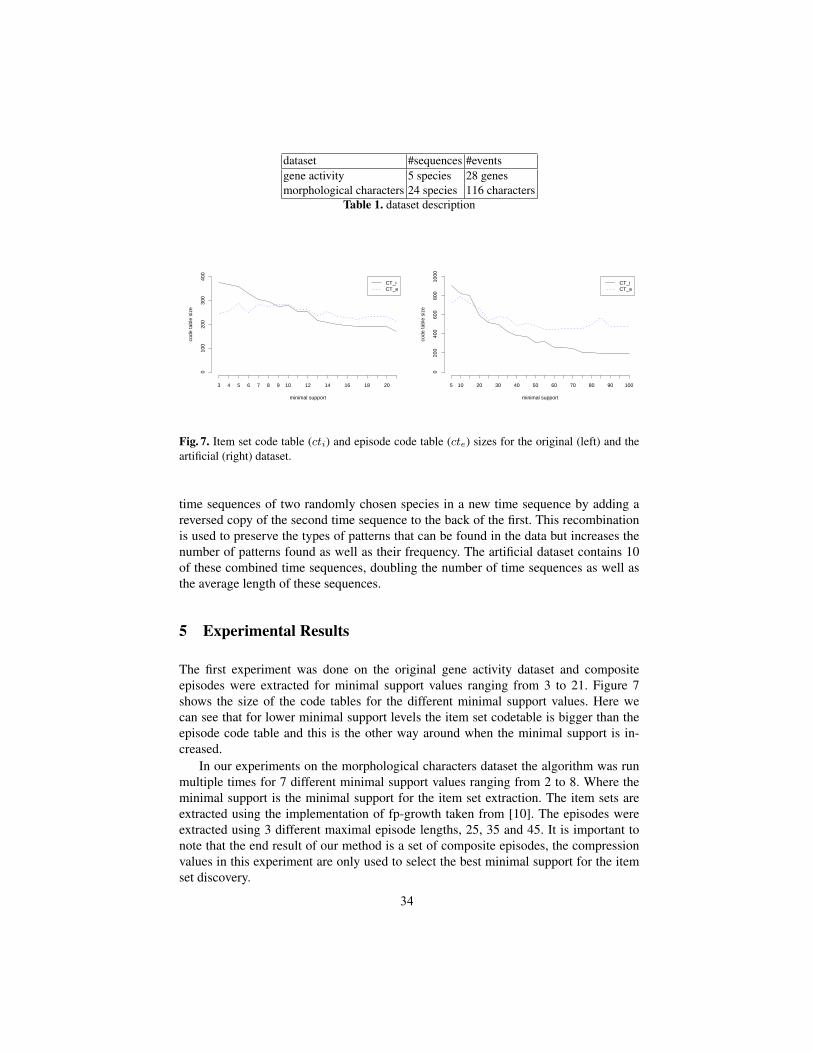
dataset #sequences #eventsgene activity 5 species 28 genesmorphological characters 24 species 116 characters

Table 1. dataset description

minimal support

code

tabl

e si

ze

3 4 5 6 7 8 9 10 12 14 16 18 20

010

020

030

040

0

CT_iCT_e

minimal support

code

tabl

e si

ze

5 10 20 30 40 50 60 70 80 90 100

020

040

060

080

010

00

CT_iCT_e

Fig. 7. Item set code table (cti) and episode code table (cte) sizes for the original (left) and theartificial (right) dataset.

time sequences of two randomly chosen species in a new time sequence by adding areversed copy of the second time sequence to the back of the first. This recombinationis used to preserve the types of patterns that can be found in the data but increases thenumber of patterns found as well as their frequency. The artificial dataset contains 10of these combined time sequences, doubling the number of time sequences as well asthe average length of these sequences.

5 Experimental Results

The first experiment was done on the original gene activity dataset and compositeepisodes were extracted for minimal support values ranging from 3 to 21. Figure 7shows the size of the code tables for the different minimal support values. Here wecan see that for lower minimal support levels the item set codetable is bigger than theepisode code table and this is the other way around when the minimal support is in-creased.

In our experiments on the morphological characters dataset the algorithm was runmultiple times for 7 different minimal support values ranging from 2 to 8. Where theminimal support is the minimal support for the item set extraction. The item sets areextracted using the implementation of fp-growth taken from [10]. The episodes wereextracted using 3 different maximal episode lengths, 25, 35 and 45. It is important tonote that the end result of our method is a set of composite episodes, the compressionvalues in this experiment are only used to select the best minimal support for the itemset discovery.

34

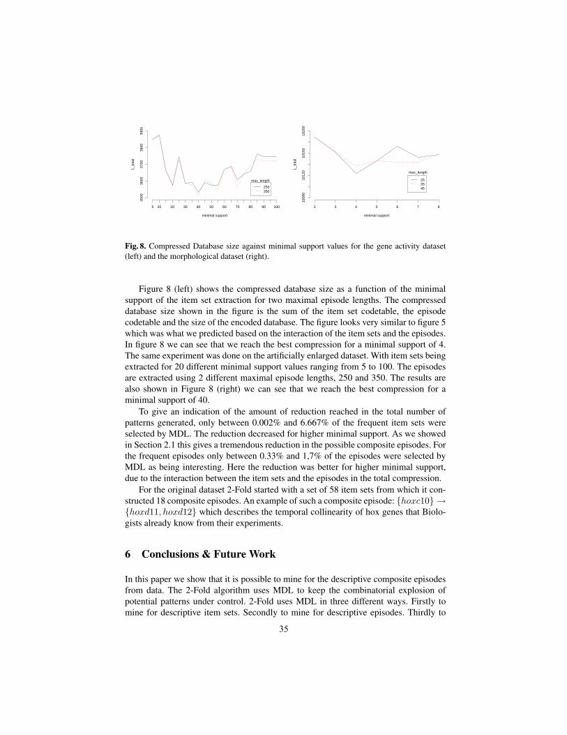
minimal support

L_to

tal

5 10 20 30 40 50 60 70 80 90 100

3500

3600

3700

3800

3900

max_length

250350

minimal support

L_to

tal

2 3 4 5 6 7 8

1008

010

120

1016

010

200

max_length

253545

Fig. 8. Compressed Database size against minimal support values for the gene activity dataset(left) and the morphological dataset (right).

Figure 8 (left) shows the compressed database size as a function of the minimalsupport of the item set extraction for two maximal episode lengths. The compresseddatabase size shown in the figure is the sum of the item set codetable, the episodecodetable and the size of the encoded database. The figure looks very similar to figure 5which was what we predicted based on the interaction of the item sets and the episodes.In figure 8 we can see that we reach the best compression for a minimal support of 4.The same experiment was done on the artificially enlarged dataset. With item sets beingextracted for 20 different minimal support values ranging from 5 to 100. The episodesare extracted using 2 different maximal episode lengths, 250 and 350. The results arealso shown in Figure 8 (right) we can see that we reach the best compression for aminimal support of 40.

To give an indication of the amount of reduction reached in the total number ofpatterns generated, only between 0.002% and 6.667% of the frequent item sets wereselected by MDL. The reduction decreased for higher minimal support. As we showedin Section 2.1 this gives a tremendous reduction in the possible composite episodes. Forthe frequent episodes only between 0.33% and 1,7% of the episodes were selected byMDL as being interesting. Here the reduction was better for higher minimal support,due to the interaction between the item sets and the episodes in the total compression.

For the original dataset 2-Fold started with a set of 58 item sets from which it con-structed 18 composite episodes. An example of such a composite episode: {hoxc10} →{hoxd11, hoxd12} which describes the temporal collinearity of hox genes that Biolo-gists already know from their experiments.

6 Conclusions & Future Work

In this paper we show that it is possible to mine for the descriptive composite episodesfrom data. The 2-Fold algorithm uses MDL to keep the combinatorial explosion ofpotential patterns under control. 2-Fold uses MDL in three different ways. Firstly tomine for descriptive item sets. Secondly to mine for descriptive episodes. Thirdly to

35

balance the first two, to ensure the discovery of descriptive composite episodes. Theexperiments show first of all that MDL performs well in all three of its tasks. Thenumber of composite episodes discovered is small enough that experts can still verifythem. Moreover, the validity of the results we discovered has been verified by domainexperts.

Acknowledgment

We would like to thank Matthijs van Leeuwen & Jilles Vreeken for their short introduc-tion on item set MDL.

References

1. Mannila, H., Toivonen, H., Verkamo, A.I.: Discovery of frequent episodes in event se-quences. Data Mining and Knowledge Discovery 1 (1997) 259–289

2. Zhang, S., Zhang, J., Zhu, X., Huang, Z.: Identifying follow-correlation itemset-pairs. In:ICDM ’06: Proceedings of the Sixth International Conference on Data Mining, Washington,DC, USA, IEEE Computer Society (2006) 765–774

3. Wang, C., Parthasarathy, S.: Summarizing itemset patterns using probabilistic models. In:KDD ’06: Proceedings of the 12th ACM SIGKDD international conference on Knowledgediscovery and data mining, New York, NY, USA, ACM Press (2006) 730–735

4. van Leeuwen, M., Vreeken, J., Siebes, A.: Compression picks item sets that matter. InFurnkranz, J., Scheffer, T., Spiliopoulou, M., eds.: PKDD. Volume 4213 of Lecture Notes inComputer Science., Springer (2006) 585–592

5. Siebes, A., Vreeken, J., van Leeuwen, M.: Itemsets that compress. In: SIAM 2006: Proceed-ings of the SIAM Conference on Data Mining, Maryland, USA (2006) 393–404

6. Bathoorn, R., Koopman, A., Siebes, A.: Reducing the frequent pattern set. In Tsumoto, S.,Clifton, C., Zhong, N., Wu, X., Liu, J., Wah, B., Cheung, Y.M., eds.: ICDM ’06: Proceed-ings of the 6th International Conference on Data Mining - Workshops. Volume 6 of ICDMworkshops., Los Alamitos, CA, USA, IEEE Computer Society (2006) 55–59

7. Grunwald, P. In: Advances in Minimum Description Length. A tutorial introduction to theminimum description length principle. MIT Press (2005)

8. Han, J., Pei, J., Yin, Y.: Mining frequent patterns without candidate generation. In Chen, W.,Naughton, J., Bernstein, P.A., eds.: 2000 ACM SIGMOD Intl. Conference on Managementof Data, ACM Press (2000) 1–12

9. Welten, M.C.M., Verbeek, F.J., Meijer, A.H., Richardson, M.K.: Gene expression and digithomology in the chicken embryo wing. Evolution & Development 7 (2005) 18–28

10. Racz, B., Bodon, F., Schmidt-Thieme, L.: On benchmarking frequent itemset mining algo-rithms. In: Proceedings of the 1st International Workshop on Open Source Data Mining, inconjunction with ACM SIGKDD. (2005)

36

Using Secondary Knowledge to SupportDecision Tree Classification of Retrospective

Clinical Data?

Dympna O’Sullivan1, William Elazmeh2, Szymon Wilk1, Ken Farion3, StanMatwin1,3, Wojtek Michalowski1, and Morvarid Sehatkar1

1 University of Ottawa, Ottawa, Canadadympna,wilk,wojtek@telfer.uottawa.ca, mseha092@site.uottawa.ca

2 Institute of Computer Science, Polish Academy of Sciences, Warsaw, Polandstan@site.uottawa.ca

3 University of Bristol, Bristol, United Kingdomelazmah@cs.bris.ac.uk

4 Faculty of Medicine, University of Ottawa, Ottawa, Canadafarion@cheo.on.ca

Abstract. Retrospective clinical data presents many challenges for datamining and machine learning. The transcription of patient records frompaper charts and subsequent manipulation of data often results in highvolumes of noise as well as a loss of other important information. In addi-tion, such datasets often fail to represent expert medical knowledge andreasoning in any explicit manner. In this research we describe applyingdata mining methods to retrospective clinical data to build a predic-tion model for asthma exacerbation severity for pediatric patients in theemergency department. Difficulties in building such a model forced usto investigate alternative strategies for analyzing and processing a ret-rospective data. This paper describes this process together with an ap-proach to mining retrospective clinical data by incorporating formalizedexternal expert knowledge (secondary knowledge sources) into the classi-fication task. This knowledge is used to partition the data into a numberof coherent sets, where each set is explicitly described in terms of thesecondary knowledge source. Instances from each set are then classifiedin a manner appropriate for the characteristics of the particular set. Wepresent our methodology and outline a set of experiential results thatdemonstrate some advantages and some limitations of our approach.

1 Introduction

In his book [1], Motulsky submits “the human brain excels at finding patternsand relationships ...”. Scientists have long exhibited an aptitude to learn and

? The support of the Natural Sciences and Engineering Research Council of Canada,the Canadian Institutes of Health Research and the Ontario Centres of Excellenceis gratefully acknowledged.

37

generalize from observations leading them to develop refined methods for de-tecting patterns and identifying coherent conjectures drawn from experience.Since their early days, intelligent computer systems have inspired scientists withtheir promising potential of supporting such research in medical domains [2].However, medical data features many difficult domain-specific characteristicsand complex properties [3]. Incompleteness (missing data), incorrectness (noise),sparseness (non-representative values), and inexactness (inappropriate parame-ter selection) make up the short list of challenges faced by any machine learningtechnique applied in the medical domain [4]. A comprehensive overview of theseand other challenges is presented in [5], where medical data is described as oftenbeing heterogeneous in source as well as in structure, and that the pervasive-ness of missing values for technical and/or social reasons can create problemsfor automatic methods for classification and prediction. Furthermore, translat-ing physicians’ interpretations based on years of clinical experience to formalmodels represents a serious and complex challenge.

An important requirement of medical problem solving or decision support ap-plications is interpretability for domain users [6]. Such a stipulation dramaticallyreduces the choice of machine learning models that can be applied to medicalproblem solving to those that can offer systematic justification and explanationof the prediction process. Such models include classifiers that estimate prob-abilities (probabilistic), classifiers that identify training examples similar to atest example (case-based), classifiers that produce rules that can be applied to agiven test example (rule-based), and classifiers that describe decisions based ona selected set of attributes (tree-based). In this work we have chosen to focus ourprediction efforts on tree-based classifiers. Decision tree classification models areespecially useful in medical applications as a result of their simple interpretationbut also as they are represented in the form typically used for describing clinicalalgorithms and practice guidelines. As such a tree-based classification model caneasily be represented in a comprehensible and transparent format if required,without the need for computer implementation.

In this work, the clinical prediction task is centered on the domain of emer-gency pediatric asthma where the goal is to develop a classification model thatcan provide an early prediction of the severity of a child’s asthma exacerba-tion. Asthma is the most common chronic disease in children (10% of Canadianpopulation), and asthma exacerbations are one of the most common reasonsfor children to be brought to the emergency department [7]. The provision ofcomputer-based decision support to emergency physicians treating asthma pa-tients has been shown to increase the overall effectiveness of health care deliveredin emergency departments [8, 9]. For a patient suffering from an asthma exac-erbation, early identification of severity (mild, moderate, or severe) is a crucialpart of the management and treatment process. Patients with a mild attack areusually discharged following a brief course of treatment (less than 4 hours) andresolution of symptoms, patients with a moderate attack receive more aggres-sive treatment over an extended observation in the emergency department (upto 12 hours), and patients with a severe attack receive maximal therapy before

38

ultimately being transferred to an in-patient hospital bed for ongoing treatment(after about 16 hours in the emergency department).

This paper discusses challenges, issues, and difficulties we face in developinga prediction model for early asthma exacerbation severity using a retrospectiveclinical data. Preliminary analysis of the data without preprocessing resulted inunacceptably low classification accuracy. These results forced a rethink of com-mon methodologies for mining retrospective clinical data. Although not partic-ularly complex, this data set is characterized by a fair amount of missing valuessuch that standard methods of feature extraction and classifier tuning fail to pro-duce acceptable performance. Furthermore, clinically-based “classifiers”, such asPRAM (section 3.1) cannot be applied due to the type of data being collected.We employ such a clinical classifier as an external method to evaluate the datawhich leads to the identification of data where PRAM can be used and “other”.We argue that such partitioning will ultimately improve the classification. Ourinvestigations led us to develop a methodology for classification that involvesidentification and formalization of expert medical knowledge specific to the clin-ical domain. This knowledge is referred to as a secondary knowledge source andits incorporation allowed us to exploit implicit domain knowledge in the datafor more fine-grained data analysis and processing. This paper demonstrates theusefulness of how to exploit this secondary knowledge to partition medical datato reduce its complexity. Our experimental evaluation demonstrates that withsuch partitioning a decision tree classifier is capable of overcoming some but notall complexities posed by this dataset. An added benefit is the ability to capturedifferent regularities that should be in asthma data according to PRAM, thusin a sense, we “extend” its interpretation.

This paper is organized as follows. In Section 2 we describe the retrospectivelycollected asthma data used in this analysis. Section 3 outlines a methodology foridentifying, formalizing and applying secondary knowledge sources with the pur-pose of harnessing and exploiting implicit domain knowledge. An experimentalevaluation of this approach is outlined in Section 4, where our results display thatthe approach can be applied with some degree of success with some limitations.We conclude with a discussion in Section 5.

2 Retrospective Clinical Dataset

The dataset used in this study was developed as part of a retrospective chartstudy conducted in 2004 at the Children’s Hospital of Eastern Ontario (CHEO),Ottawa, Canada. The study includes patients who visited the hospital’s emer-gency department from 2001 to 2003 for treatment of an asthma exacerbation.To illustrate the underlying structure of the data, we present the workflow bywhich asthma patients are processed in the emergency department (Figure 1).The workflow shows that a patient is evaluated multiple times by multiple care-givers at variable time intervals. This information is documented on the patientchart with varying degrees of completeness. Furthermore, some aspects of evalua-tion are objective and therefore reliable measures of the patient’s status, however

39

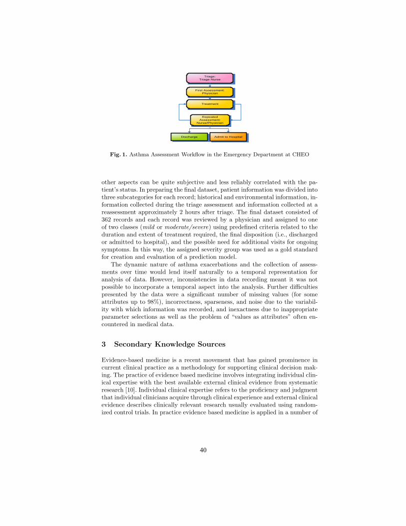
Triage:Triage Nurse

Treatment

Repeated Assessment:

Nurse/Physician

Admit to HospitalDischarge

First Assessment:Physician

Fig. 1. Asthma Assessment Workflow in the Emergency Department at CHEO

other aspects can be quite subjective and less reliably correlated with the pa-tient’s status. In preparing the final dataset, patient information was divided intothree subcategories for each record; historical and environmental information, in-formation collected during the triage assessment and information collected at areassessment approximately 2 hours after triage. The final dataset consisted of362 records and each record was reviewed by a physician and assigned to oneof two classes (mild or moderate/severe) using predefined criteria related to theduration and extent of treatment required, the final disposition (i.e., dischargedor admitted to hospital), and the possible need for additional visits for ongoingsymptoms. In this way, the assigned severity group was used as a gold standardfor creation and evaluation of a prediction model.

The dynamic nature of asthma exacerbations and the collection of assess-ments over time would lend itself naturally to a temporal representation foranalysis of data. However, inconsistencies in data recording meant it was notpossible to incorporate a temporal aspect into the analysis. Further difficultiespresented by the data were a significant number of missing values (for someattributes up to 98%), incorrectness, sparseness, and noise due to the variabil-ity with which information was recorded, and inexactness due to inappropriateparameter selections as well as the problem of “values as attributes” often en-countered in medical data.

3 Secondary Knowledge Sources

Evidence-based medicine is a recent movement that has gained prominence incurrent clinical practice as a methodology for supporting clinical decision mak-ing. The practice of evidence based medicine involves integrating individual clin-ical expertise with the best available external clinical evidence from systematicresearch [10]. Individual clinical expertise refers to the proficiency and judgmentthat individual clinicians acquire through clinical experience and external clinicalevidence describes clinically relevant research usually evaluated using random-ized control trials. In practice evidence based medicine is applied in a number of

40

ways, including, through the use of clinical practice guidelines, specialty-specificliterature and clinical scoring systems.

In this research, we utilize external clinical evidence to support the classifica-tion task. The incorporation of a secondary knowledge source into classificationleads us to define a three step approach to mining retrospective clinical data. Inthe first step relevant medical evidence is identified, for example in the form of aclinical practice guideline for the particular clinical domain. The second step is toformalize the medical evidence so it can be applied to available data. The thirdstep involves developing a framework that makes use of the evidence to supportthe automatic classification task. The advantage of integrating such knowledgeis that it allows for more effective and natural organization of information alongexisting and important data characteristics. As such secondary knowledge canbe viewed as a proxy for an expert built classifier and may be incorporated toimprove the predictive accuracy of the automatic classification task.

3.1 Secondary Knowledge Sources for Pediatric Asthma

The secondary knowledge source identified as relevant for our retrospectiveasthma data is the Preschool Respiratory Assessment Measure (PRAM) asthmaindex [11]. PRAM provides a discriminative index of asthma severity for preschoolchildren. It is based on five clinical attributes commonly recorded for pediatricasthma patients, suprasternal indrawing, scalene retractions, wheezing, air entryand oxygen saturation. PRAM is based on a 12 point scale (see Table 1) and iscalculated using scores of 0, 1, 2, and 3. These scores are assigned to attributesdepending on the presence or absence of values as well as observed increasing ordecreasing values of attributes. PRAM has been clinically validated as a reliableand responsive measure of the severity of airway obstruction. A patient witha PRAM score of 4 or less is considered to have a mild exacerbation, a scorebetween 5 and 8 corresponds to a moderate exacerbation, and a score of 9 orhigher corresponds to a severe exacerbation.

In order to identify if the PRAM scoring system was appropriate secondaryknowledge, the retrospective asthma dataset was analyzed for the presence ofPRAM attributes. It was found that four of the five PRAM attributes werepresent in our data and values for these attributes may be collected twice foreach record, once at triage and again at reassessment. The next step of ourapproach was to formalize the secondary knowledge source so that it could beapplied to the classification task. This process is described in the next subsection.

3.2 Formalizing Secondary Knowledge Sources for Classification

The formalization of the secondary knowledge source involved determining amapping from the set of attributes outlined by PRAM to a subset of attributesfrom the retrospective asthma data and an associated assignment of scores forattribute values. This was necessary as not all attributes required to calculatethe PRAM score were present in the retrospective asthma data, and for someother attributes a 1:1 mapping did not exist. Specifically, the retrospective data

41

Table 1. PRAM Scoring System

Signs 0 1 2 3

Suprasternal absent presentindrawing

Scalene absent presentretractions

Wheezing absent expiratory inspiratory Audibleand without

expiratory stethoscope/absent withno air entry

Air normal decreased widespread absent/entry bases decrease minimal

Oxygen ≥95% 92-95% <92%saturation

did not contain an attribute corresponding with “Suprasternal Indrawing”, and“Wheezing” was captured using two attributes in the retrospective data, in-spiratory wheezing and expiratory wheezing. Also, the PRAM scoring systemdescribes “Air Entry” using four values (normal, decreased bases, widespreaddecrease and absent/minimal), whereas our data defined air entry as either good(i.e., normal) or reduced. Therefore the formalized mapping was developed inconjunction with a domain expert (emergency physician), and the rules devisedfor mapping attributes used by the PRAM system to attributes in our data andtheir corresponding score assignments are shown in Table 2.

3.3 Building a Classifier by a Secondary Knowledge Source

The final step of our approach was to use secondary knowledge to build a modelfor predicting asthma severity. In the retrospective asthma data a decision (classlabel) is recorded for each patient along with clinical and historical information.This class is the final outcome for the patient as recorded in the patient chart(not the result of the assessment at the 2-hour point) and indicates whetherthe patient has suffered a mild or moderate/severe exacerbation. Using the at-tributes, values and associated scores mapped from the PRAM scoring systemwe calculated a PRAM score for each patient in the dataset. This score hadpossible values between 0 and 12, where a score of less than 5 indicated a mildexacerbation and a score of greater than 5 indicated a moderate/severe exacer-bation. (In our data the moderate and severe categories outlined by PRAM arecollapsed into one group, moderate/severe). The score is then compared with theclass label for each record in the dataset and the set of patients who comply withthe PRAM scoring system are identified. The assignment of PRAM scores allowsfor the dataset to be partitioned into instances for which all PRAM attributeswere present and thus a complete and correct PRAM score could be calculatedand instances for which only a partial or no PRAM score could be calculated due

42

Table 2. Mapping PRAM attributes and scores

Attribute(s) Value(s) Score

Oxygen Saturation Greater than 95% 0Oxygen Saturation Greater than 92% and Less than 95% 1Oxygen Saturation Greater than 88% and Less than 92% 2Oxygen Saturation Less than 88% 3

Air Entry Good 0Air Entry (class = mild) Reduced 1Air Entry (class = other) Reduced 3

Retractions AND Air Entry Absent AND Good 0Retractions AND Air Entry Absent AND Reduced 1Retractions AND Air Entry Absent AND “Missing” 2

Retractions Present 2

Expiratory AND Inspiratory Wheeze Absent AND Absent 0Expiratory AND Inspiratory Wheeze Present AND Absent 1Expiratory AND Inspiratory Wheeze Present AND Present 2Expiratory AND Inspiratory Wheeze Absent AND Present Undefined

to the absence of values for the PRAM attributes. PRAM attributes may be col-lected at two stages in the asthma workflow (triage and reassessment), howeveranalysis of our data demonstrated that such attributes were more likely to becollected at reassessment (there were many missing values for triage attributes)and as such the dataset was partitioned using the larger set of reassessed values.This resulted in a dataset with 147 instances for which the PRAM score wascomplete and correct, 206 instances where only a partial or no PRAM scorecould be calculated due to missing values and 9 instances for which the scorecalculated by PRAM and the class label completely disagreed. These 9 caseswere considered outliers and deleted from the dataset for evaluation.

4 Experimental Evaluation

4.1 Experimental Design

Our evaluation reports results from a number of experiments involving the ret-rospective asthma dataset where each experiment involved building a decisiontree using the J48 decision tree classifier in Weka[12] to classify data. The firstexperiment involved building a classifier on the entire dataset prior to any ap-plication of secondary knowledge. These results serve as a baseline for classifierperformance upon which to evaluate all subsequent results. In the next experi-ment secondary knowledge in the form of the PRAM scoring system was appliedto partition the dataset into two sets, one containing PRAM complete and cor-rect instances and one containing PRAM partial or incomplete instances. Thepurpose of this experiment is to demonstrate that the incorporation of secondaryknowledge into the classification tasks allows for enhanced representation of data

43

which results in reducing the complexity of the retrospective clinical dataset forclassification. In the final experiment we applied feature selection to the com-plete original data set twice, once using automatic feature selection (availablein Weka), and a second time by manually selecting combinations of expertlyselected attributes and removing the remaining attributes. The function of thisexperiment was to show that neither automatic or expert feature selection canidentify and reduce complexities in the data as efficiently as a classifier thatincorporates secondary or expert medical knowledge, selects important featuresand partitions data into sets of similar characteristics.

For each experiment we report classifier performance in terms of percentagesof Sensitivity (Sens) and Specificity (Spec), Predictive Accuracy (Acc) and AreaUnder the Curve (AUC) on the positive class. Sensitivity (the true positive rate)measures how often the classifier finds a set of positive examples. For instance inthis research we consider moderate/severe to be the critical/positive class, there-fore the sensitivity of moderate/severe measures how often the classifier correctlyidentifies patients suffering moderate/severe asthma exacerbations. Specificity (1- false positive rate) measures how often what the classifier finds, is indeed whatit was looking for. Therefore the specificity of the positive class (moderate/severe)measures how often what the classifier predicts is indeed a patient with a moder-ate/severe asthma exacerbation. Analyzing the trade-off between sensitivity andspecificity is common in medical domains and is analogous to Receiver OperatingCharacteristics (ROC) analysis [13, 14] used in machine learning [15].

In addition we report accuracy and AUC where accuracy is the rate at whichthe classifier classifies patients (in both classes) correctly while AUC representsthe probability that the classifier will rank a randomly chosen positive instancehigher than a randomly chosen negative instance [16]. Hence AUC measuresthe classifier’s ability to discriminate the positive class from the negative class.In our experiments, we aim to analyze decision tree performance by measuringits ability to discriminate each positive patient with a moderate/severe asthmaexacerbation. For a given classifier and positive class, an ROC curve [15, 16] plotsthe true positive rate against the rate of false positives produced by the classifieron the test data. The points along the ROC curve are produced by varyingthe classification threshold from most positive classification to most negativeclassification and the AUC of a classifier is the area under the ROC curve [16].For this reason as well as the relatively small size of the dataset we evaluate theclassifier for each patient in the dataset using leave-one-out cross-validation.

4.2 Classifying the Entire Dataset

The first experiment involved building a decision tree on the original datasetof 362 instances. The results of this experiment are shown in the first row ofTable 3 and demonstrate that the retrospective clinical dataset is complex andthat good classification accuracy is difficult to achieve without performing somedegree of data preprocessing. We include these results as a baseline by which tomeasure subsequent classifier performance.

44

4.3 Classifying PRAM and non-PRAM Sets

In this experiment the dataset was partitioned by applying the formalized map-ping from PRAM scoring system to attributes from the retrospective asthmadataset. This resulted in the dataset being partitioned into those that werePRAM complete and correct (PRAM set) and those that were either PRAMpartial or incomplete (non-PRAM set). A decision tree was built for each setand the results are shown in the last two rows of Table 3. Also included forreference purposes are the results for the entire dataset in the first row.

Table 3. Decision Trees built on PRAM and non-PRAM sets

Set Size Sens Spec Acc AUC

Entire 362 73 63 69 69

PRAM Set 147 93 96 95 98

Non-PRAM Set 206 89 53 74 77

From Table 3 we observe that splitting the datset into different sets based onformalized secondary knowledge increases classification accuracy of the PRAMset. For the non-PRAM set classification improves in terms of Sensitivity, Ac-curacy and AUC. In particular sensitively on the PRAM set increases by 20%from the baseline. In addition a large gain in AUC from the baseline reflectsthe increased probability that a positive example is ranked higher than a neg-ative example. In fact, when the decision tree is supplemented with secondaryknowledge (the PRAM set) we gain an increase in AUC, and when secondaryknowledge cannot be so easily applied (non-PRAM set), the performance onlyimproves marginally on that of the baseline. These results demonstrate that theincorporation of formalized secondary knowledge sources can help with classifi-cation in such domains unraveling the concept to be learned by the decision treeand thus reducing the overall complexity of the dataset by exploiting domainknowledge implicitly present in the data. The results represent an overall im-provement on previous research into classification of clinical data with tree-basedclassifiers [8, 9].

However from the results in Table 3 we also observe a decrease of 10% inspecificity between the Non-PRAM set and the baseline. This performance isinadequate in terms of achieving a balance between high sensitivity and highspecificity. We note however that in terms of the problem domain high sensitivityand low specificity on the positive class translates to the fact that the classifieris very accurate in identifying moderate/severe patients and recommending theyare kept for an extended time in the emergency department, however at thesame time the classifier is overconservative in recommending that mild patientsare kept for longer than usual stays. Such direction of classification a less seriouserror than one occurring in the opposite situation.

45

4.4 Automatic and Expert-Driven Feature Selection

It is acceptable to state that a reduction in dimensionality of data can reducethe complexity of underlying concepts that it may represent. The purpose of thisexperiment is to demonstrate that data complexity in this domain requires morethan dimensionality reduction to reduce its complexity. We compare results ob-tained from applying automatic and expert-driven feature selection methods tothose obtained by partitioning the data according to PRAM secondary knowl-edge. Automatic feature selection is based on standard methods used by the datamining community and are available in the Weka software. The expert-drivenfeature selection methods are based on selecting attributes observed to useful toclassification from our repeated experiments and by an expert and those out-lined by the PRAM scoring system. 10 methods of feature automatic selectionwere applied to the dataset where each was used in conjunction with a decisiontree for classification. The results for the best four methods are shown in rows1-4 of Table 4. Comparing the results for automatic feature selection to thosefor the baseline as outlined in Table 3 we can conclude it is not successful inreducing the complexity of the dataset. In general results do not display anyimprovement in classification except in the case where a wrapper using a NaiveBayes classifier for optimization is used for feature selection. Here we note anincrease in AUC, however this is at the expense of a large decrease in specificity.In applying expert feature selection, we built one classifier using all data recordsof attributes collected during the reassessment only and another classifier usingonly the attributes that were mapped from the PRAM scoring system while stillusing all instances available in the dataset. The results for these two experimentsare shown in rows 5-6 of Table 4. Again comparing these results to those outlinedfor the baseline in Table 3 we observe no significant improvement.

However, by comparing the results from Table 4 to those for classificationon the PRAM and non-PRAM sets in Table 3 a number of important conclu-sions can be drawn. Partitioning data into different sets for classification basedon secondary knowledge results in much improved classification that of usingeither automatic or expert feature selection. Augmenting the developed classi-fier with external knowledge allows for more effective classification by exploitingunderlying domain knowledge in the dataset and by organizing data accordingto these concepts. Such classification accuracy cannot be captured by a classi-fication model developed on the data alone. The partitioning of data does notreduce the dimensionality of the dataset like traditional methods for classifica-tion such as feature selection, however it manages to reduce the complexity ofthe dataset by using secondary knowledge to identify more coherent sets intowhich data more naturally fits.

The intention is to use the classification results from the PRAM and non-PRAM sets from Table 3 to implement a prediction model for asthma severity.This can be achieved in a number of ways. One option is to develop a metaclas-sifer that could learn to direct new instances to either the model built on thePRAM set or the model built on the non-PRAM set. For such a metaclassifiervalues of PRAM attributes alone may be sufficient to make the decision or it

46

Table 4. Automatic and Expert Feature Selection

Feature Selection Mode Mode Size Sens Spec Acc AUC

Information Gain Automatic 362 72 63 68 69

Chi-squared Automatic 363 72 63 68 69

Combinatorial Automatic 362 72 65 69 71

Wrapper with Naive Bayes Automatic 362 71 60 70 77

On All Attributes Expert 362 72 66 70 73

On Only PRAM Attributes Expert 362 77 78 70 71

may be necessary to develop a method by which unseen patients can be relatedto the sets (PRAM and non-PRAM) we identify in the dataset. Alternatively thepredictions from both sets could be combined to perform the prediction task.One option is to use a voting mechanism, another is to build these classifiersin a manner that produce rankings of the severity of the exacerbation. Withsuch a methodology the classifier with the highest ranking provides a better in-sight into the condition. However, such an approach introduces additional issuesin terms of interpretations and calibrations of ranks and probabilities. Such astudy remains as part of our future research directions.

5 Discussion

We have introduced an approach to mining complex retrospective clinical databy incorporating secondary knowledge to supplement the classification task byreducing the complexity of the dataset. The methodology involves identificationof a secondary knowledge source suitable for the clinical domain, formalization ofthe knowledge to analyze and organize data according to the underlying principleof the secondary knowledge, and incorporation of the secondary knowledge intothe chosen classification model. In this research we concentrated on classifyinginformation using a decision tree to satisfy the requirement that classificationshould be easily interpreted by domain users. From our experimental results wedraw a number of conclusions. Firstly we have demonstrated that domain knowl-edge is implicit in the data as the dataset partitions naturally into two sets forclassification with the application of a formalized mapping from the PRAM scor-ing system. This is in spite of the fact that the mapping was inexact; our datasetonly contained four of the five attributes outlined by PRAM and some attributevalues had slightly different representations. In such a way the application ofsecondary knowledge reduces the complexity of the dataset by allowing for theexploitation of underlying domain knowledge to supplement data analysis, rep-resentation and classification. As outlined, this approach is more successful thantraditional methods for reducing data complexity such as feature selection whichfail to capture a measure of the expert knowledge implicit in the retrospectivelycollected data. A further advantage of the approach was demonstrated by theability of the secondary knowledge to help identify outlier examples in the data.

47

However, the results are still somewhat disappointing in terms of achieving abalance acceptable in medical practice between high sensitivity and high speci-ficity in the non-PRAM set. We believe that a high proportion of missing valuesin this set is causing difficulties for the classification model. This issue remainsan open problem for future research. In other future work we are interested infurther investigating attributes used by the PRAM system and to test whetherall attributes used by PRAM are necessary for enhanced classification.

References

1. Motulsky, H.: Intuitive Biostatistics. Oxford University Press, New York (1995)2. Ledley, R.S., Lusted, L.B.: Reasoning foundations of medical diagnosis. Science

130 (1959) 9–213. Mullins, I.M., Siadaty, M.S., Lyman, J., Scully, K., Garrett, C.T., Miller, W.G.,

Muller, R., Robson, B., Apte, C., Weiss, S., Rigoutsos, I., Platt, D., Cohen, S.,Knaus, W.A.: Data mining and clinical data repositories: Insights from a 667,000patient data set. Computers Biology and Medicine 36(12) (2006) 1351–77

4. Magoulas, G.D., Prentza, A.: Machine learning in medical applications. LectureNotes in Computer Science 2049 (2001) 300–307

5. Cios, K.J., Moore, G.W.: Uniqueness of medical data mining. A. I. in medicine26(1-2) (2002) 1–24

6. Lavrac, N.: Selected techniques for data mining in medicine. Artificial Intelligencein Medicine 16(1) (1999) 3–23

7. Lozano, P., Sullivan, S., Smith, D., Weiss, K.: The economic burden of asthma inus children: estimates from the national medical expenditure survey. The Journalof allergy and clinical immunology 104(5) (1999) 957–63

8. Kerem, E., Tibshirani, R., Canny, G., Bentur, L., Reisman, J., Schuh, S., Stein, R.,Levison, H.: Predicting the need for hospitalization in children with acute asthma.Chest 98 (1990) 1355–1361

9. Lieu, T.A., Quesenberry, C.P., Sorel, M.E., Mendoza, G.R., Leong, A.B.:Computer-based models to identify high-risk children with asthma. AmericanJournal of Respiratory and Critical Care Medicine 157(4) (1998) 1173–80

10. Sackett, D., Rosenberg, W., Muir Gray, J., Haynes, R., Richardson, W.: Evidencebased medicine: what it is and what it isn’t. British Medical Journal (1996)

11. Chalut, D.S., Ducharme, F.M., Davis, G.M.: The preschool respiratory assessmentmeasure (pram): A responsive index of acute asthma severity. Pediatrics 137(6)(2000) 762–768

12. Witten, I.H., Frank, E.: Data mining: Practical machine learning tools and tech-niques. (2005)

13. Sox, H.C.J., Blatt, M.A., Higgins, M.C., Marton, K.I.: Medical Decision Making.(Boston, 1998)

14. Faraggi, D., Reiser, B.: Computer-based models to identify high-risk childrenwith asthma. American Journal of Respiratory and Critical Care Medicine 157(4)(1998) 1173–80

15. Provost, F., Fawcett, T.: Analysis and visualization of classifier performance: com-parison under imprecise class and cost distributions. The Third InternationalConference on Knowledge Discovery and Data Mining (1997) 34–48

16. Fawcett, T.: Roc graphs: Notes and practical considerations for data mining re-searchers (2003) Technical Report HPL-2003-4, HP Labs.

48

Evaluating a Trading Rule Mining Method based on Temporal Pattern Extraction

Hidenao Abe1, Satoru Hirabayashi2, Miho Ohsaki3, and Takahira Yamaguchi4

1Department of Medical Informatics, Shimane University, School of Medicine abe@med.shimane-u.ac.jp

2Graduate School of Science and Technology, Keio University and_joy@ae.keio.ac.jp

3Faculty of Engineering, Doshisha University mohsaki@mail.doshisha.ac.jp

4Faculty of Science and Technology, Keio University yamaguti@ae.keio.ac.jp

Abstract. In this paper, we present an evaluation of the integrated temporal data mining environment for trading dataset from the Japanese stock market. Temporal data mining is one of key issues to get useful knowledge from databases. However, users often face difficulties during such temporal data mining process for data pre-processing method selection/construction, mining algorithm selection, and post-processing to refine the data mining process as shown in other data mining processes. To get more valuable rules for experts from a temporal data mining process, we have designed an environment which integrates temporal pattern extraction methods, rule induction methods and rule evaluation methods with visual human-system interface. After implementing this environment, we have done a case study to mine temporal rules from a Japanese stock market database for trading. The result shows the availability to find out useful trading rules based on temporal pattern extraction

1 Introduction

In recent years, KDD (Knowledge Discovery in Databases) [3] has been widely known as a process to extract useful knowledge from databases. In the research field of KDD, ‘Temporal (Time-Series) Data Mining’ is one of important issues to mine useful knowledge such as patterns, rules, and structured descriptions for a domain expert. However, huge numerical temporal data such as stock market data, medical test data, and sensor data have been only stored to databases.

Besides, many temporal mining schemes such as temporal pattern extraction methods and frequent itemset mining methods have been proposed to find out useful knowledge from numerical temporal databases. Although each method can find out partly knowledge of each suggested domains, there is no systematic framework to utilize each given numerical temporal data through whole of the KDD process.

To above problems, we have developed an integrated temporal data mining environment, which can apply numerical temporal data to find out valuable

49

knowledge systematically. The environment consists of temporal pattern extraction, mining, mining result evaluation support system to attempt numerical temporal data from various domains.

In this paper, we present an evaluation of the integrated temporal data mining environment with Japanese stock market data. Then, we discuss about the availability of the temporal rule mining process based on temporal pattern extraction.

2 Related Work

Many efforts have been done to analyze temporal data at the field of pattern recognitions. Statistical methods such as autoregressive model and ARIMA (AutoRegressive Integrated Moving Average) have been developed to analyze temporal data, which have linearity, periodicity, and equalized sampling rate. As signal processing methods, Fourier transform, Wavelet, and fractal analysis method have been also developed to analyze such well formed temporal data. These methods based on mathematic models restrict input data, which are well sampled. However, temporal data include ill-formed data such as clinical test data of chronic disease patients, purchase data of identified customers, and financial data based on social events. To analyze these ill-formed temporal data, we take another temporal data analysis method such as DTW (Dynamic Time Wrapping)[1], temporal clustering with multiscale matching [5], and finding Motif based on PAA (Piecewise Approximation Aggregation) [6].

To find out useful knowledge to decide orders for stock market trading, many studies have done. For example, temporal rule induction methods such as Das’s framework [2] have been developed. Frequent itemset mining methods are also often attempt to the domain [15]. Although they analyze the trend of price movement, many trend analysis indices such as moving average values, Bolinger band signals, MACD signals, RSI and signals based on balance table are often never considered. In addition, these studies aim not to find out decision support knowledge, which directly indicates orders for stock market trading, but useful patterns to think better decision by a domain expert. Therefore, the decision support of trading order is still costly task even if a domain expert uses some temporal data analysis methods. The reason of this problem is that decision criteria of trading called anomaly are obtained from very complex combination of many kinds of indices related to the market by domain experts.

3 An integrated temporal data mining environment

Our temporal data mining environment needs temporal data as input. Output rules are if-then rules, which have temporal patterns or/and ordinal clauses, represented in A=x, A<=y, and A>z. Combinations of extracted patterns and/or ordinal clauses can be obtained as if-then rules by a rule induction algorithm. Fig. 1 illustrates a typical output it-then rule visualized with our temporal data mining environment.

50

IF:courses of observation period

THEN:course of prediction period

Test item A

Test item C

Test item B

Test item A

Fig. 1. Typical output if-then rule, which consists of patterns both its antecedent and its consequent.

To implement the environment, we have analyzed temporal data mining frameworks [2, 10]. Then, we have identified procedures for pattern extraction as data pre-processing, rule induction as mining, and evaluation of rules with visualized rule as post-processing of mined result. The system provides these procedures as commands for users. At the same time, we have designed graphical interfaces, which include data processing, validation for patterns on elemental sequences, and rule visualization as graphs. Fig. 2 shows us a typical system flow of this temporal data mining environment.

Time-series data

Pre-Processing

Mining

Visualizing as graphs

Cleaning

EqualizingSampling

cycle

Integration

Prediction of

interest

Clustering

Interpolation

Rule Induction

Post-processing

Sorting with an index

Visualized Rules

Setting up an index for sorting.

Input rule evaluations

Procedures for structuring a dataset

Pattern Extraction

Attribute Selection

Setting up the mining targetand observation

period.Evaluating patterns

Visualizing extracted patterns

• Time-series data pre-processing• Selecting Mining algorithms• Rule & Data visualization• Rule evaluation• Database operations

Commands for users

Validation onraw data

Extractingsub-sequences

Fig. 2. A system flow view of the integrated temporal data mining environment.

51

3.1 Details of procedures to mine temporal rules

We have identified procedures for temporal data mining as follows: Data pre-processing

- pre-processing for data construction - temporal pattern extraction - attribute selection

Mining - rule induction Post-processing of mined results

- visualizing mined rule - rule selection - supporting rule evaluation

Other database procedures - selection with conditions - join

As data pre-processing procedures, pre-processing for data construction procedures

include data cleaning, equalizing sampling rate, interpolation, and filtering irrelevant data. Since these procedures are almost manual procedures, they strongly depend on given temporal data and a purpose of the mining process. Temporal pattern extraction procedures include determining the period of sub-sequences and finding representative sequences with a clustering algorithm such as K-Means, EM clustering and the temporal pattern extraction method developed by Ohsaki et al. [12]. Attribute selection procedures are done by selecting relevant attributes manually or using attribute selection algorithms [7].

At mining phase, we should choose a proper rule induction algorithm with some criterion. There are so many rule induction algorithms such as Version Space [9], AQ15 [8], C4.5 rule [13], and any other algorithm. To support this choice, we have developed a tool to construct a proper mining application based on constructive meta-learning called CAMLET. However, we have taken PART [4] implemented in Weka [16] in the case study to evaluate improvement of our pattern extraction algorithm.

To predict class of a test dataset with learned a classification model, the system should formally predict pattern symbols of the test dataset using some classification learning method L based on the training dataset as shown in Figure 3.

52

tDatasets with Temporal PatternsDatasets with Temporal Patterns

tDatasets without Temporal PatternsDatasets without Temporal Patterns

Training data

tDatasets without Temporal PatternsDatasets without Temporal Patterns

Pattern extractionwith clustering

tDatasets with Temporal PatternsDatasets with Temporal Patterns

Test data

Predicting patternswith classification

Learning classificationmodel with L.

Fig. 3. The process to obtain a test dataset based on temporal patterns of a training dataset using classification learning algorithm.

To validate mined rules correctly, users need readability and ease for understand about mined results. We have taken 39 objective rule evaluation indexes to select mined rules [11], visualizing and sorting them depended on users’ interest. Although these two procedures are passive support from a viewpoint of the system, we have also identified active system reaction with prediction of user evaluation based on objective rule evaluation indexes and human evaluations.

Other database procedures are used to make target data for a data mining process. Since the environment has been designed based on open architecture, these

procedures have been able to develop separately. To connect each procedure, we have only defined input/output data format.

4 Evaluating Temporal Rule Mining Performances with the Integrated Temporal Data Mining Environment

After implementing the integrated temporal data mining environment described in Section 3, we have done a case study on Japanese stock market database.

In this case study, we firstly gathered temporal price data and its trend index values through Kaburobo SDK [17]. Then, using the environment, we evaluated the performance of if-then rules based on temporal patterns. Finally, with regarding to the results, we discuss about the availability of our temporal rule mining based on temporal pattern extraction.

53

4.1 Description about Temporal Datasets

Using Kaburobo SDK, we got four price values, trading volume, and 13 trend index values as shown in Table 1. Excepting DMI, volume ratio, and momentum, the trend indices are defined as trading signals: buy and sell. The attribute values of these indices are converted from 1.0 to -1.0. Thus, 0 means nothing to do (or hold on the stock) for these attributes.

Table 1. The descripiton about attributes from Kaburobo SDK.

Buy: if , Sell: ifWhere ,

Ichimoku4

Buy: ifSell: if

Ichimoku3

Buy: if , Sell: ifWhere

Ichimoku2

Buy: if , Sell: ifWhere

Ichimoku1

Momentum

RSI

volumeRatio

Buy: if , Sell: ifWhere ,

,

DMI

Buy: if Sell: ifWhere ,

MACD

Buy: if , Sell: if HLband

Buy: if , Sell: if Envelope

Buy: if , Sell: if where Bolinger Band

Volume of the day ( ) Volume

Closing price of the day ( )closing

Lowest price of the day ( )low

Highest price of the day ( )high

Buy: if ,Sell: ifWhere , and

opening price of the day ( )

Description

openingRAW

Moving AverageTREND

INDICES

Attribute name

00 11 >−∩<− −− tttt LMASMALMASMA13/)( 121 −− +++= tttt CCCSMA K 26/)( 251 −− +++= tttt CCCLMA K

05.0)2( ×+≥ σtt MAC 05.0)2( ×−≤ σtt MAC

)05.0( ×+≥ ttt MAMAC )05.0( ×−≤ ttt MAMAC

daystt HighLineC 10−>daystt LowLineC 10−<

00 9)1(19 <−∩>− −−−− daysttdaystt AvgMACDMACDAvgMACDMACD

daystdaystt EMAEMAMACD 2612 −− −= ))(1/2( 111 −−− −++= tttt EMACrangeEMAEMA

tC

tO

tH

tL

tV

00 11 <−∩>− −− tttt MDIPDIMDIPDI

∑ ∑−= −=

− ×÷−=t

nti

t

ntiiii TRHHPDI 100)( 1 ∑ ∑

−= −=− ×÷−=

t

nti

t

ntiiii TRLLMDI 100)( 1

100)}/(){(,25,25,25,25

×++= ∑∑∑∑=−=<−==−=>−=

t

LHtii

t

LHtii

t

LHtii

t

LHtiit

iiiiiiii

VVVVVR

∑∑>−=

−<−=

−−−

+−−−=t

CCtiii

t

CCtiiit

iiii

CCCCRSI11 ,13

1,13

1 }1)(/)(/{100100

10−−= ttt CCM

daysttdaystt RLCRLC 991 −−− >∩< daysttdaystt RLCRLC 991 −−− <∩>))min()(max(9 iidayst LHaverageRL +=− ),7,8( ttti K−−=

00 11 >−∩<− −− tttt MDIPDIMDIPDI

))min()(max(26 iidayst LHaverageRL +=− ),24,25( ttti K−−=daysttdaystt RLCRLC 26261 −−− >∩< daysttdaystt RLCRLC 26261 −−− <∩>

00 11 <−∩>− −− tttt LMASMALMASMA

00 9)1(19 >−∩<− −−−− daysttdaystt AvgMACDMACDAvgMACDMACD

daystdaystdaystdaystdaystdayst RLRLRLRLRLRL 2626)1(9)1(26)1(9)2(26)2( −−−−−−−−−−− <∩>∩<daystdaystdaystdaystdaystdayst RLRLRLRLRLRL 2626)1(9)1(26)1(9)2(26)2( −−−−−−−−−−− >∩<∩>

2626 21 −− >∩> tttt ASCASC 2626 21 −− <∩< tttt ASCASC)(1 269 daystdaystt RLRLmedianAS −− −= 2/))min()(max(2 iit LHAS −= ),50,51( ttti K−−=

25/)( 241 −− +++= tttt CCCMA K

)}(),(),max{( 11 ttttttt LHLCCHTR −−−= −−

We obtained temporal data consists of the above mentioned attributes about five

financial companies and four telecommunication companies as follows: Credit Saison (Saison), Orix, Mitsubishi Tokyo UFJ Financial Group (MUFJFG), Mitsui Sumitomo Financial Group (MSFG), Mizuho Financial Group (MizuhoFG), NTT, KDDI, NTT Docomo, and Softbank. The period, which we have collected from the temporal stock data, is from 5th January 2006 to 31st May 2006. For each day, we have made decisions as the following: the decision is if the closing value rises 5% within 20 days then 'buy', otherwise if the closing value falls 5% within 20 days then 'sell', otherwise 'hold'. We set these decisions as the class attribute to each target instance. Table 2 shows the class distributions about the nine stocks for the period.

54

Table 2. The distributions of decisions of the nine stocks during the five months.

Finance Buy sell Telecom. buy sell Saison 37 53 NTT 27 32 Orix 43 40 KDDI 42 39 MUFJFG 0 50 NTTdocomo 19 29 MSFG 6 27 Softbank 23 69 MizuhoFG 38 31

For each gathered temporal data of the nine stocks, the system extracted temporal

patterns for each attribute. Then, the symbols of each pattern and the decision of each day joined as each instance of the target dataset as illustrated in Figure 4.

Fig. 4. An illustration of the process to obtain target datasets from temporal data

t

Price / Technical Index values

Decision point

t

Clustring each items& join decisions

…

Price / Technical Index pattern symbols

Target DatasetTarget Dataset

Sub-Sequenced DataSub-Sequenced Data

Dataset for Temporal Pattern ExtractionDataset for Temporal Pattern Extraction

Decision

Sub-Sequence

SeparatingEach Index

4.2 Mining results of the nine temporal stock data

To extract temporal patterns, we have used K-Means and EM algorithm, which are implemented in Weka. Then, to predict temporal pattern of each test dataset, we have used Boosted C4.5 [14], which is also implemented in Weka.

As shown in Table 3, predicting temporal patterns for test dataset are succeeded, because the accuracies of the nine dataset are satisfactory high scores as a classification task.

55

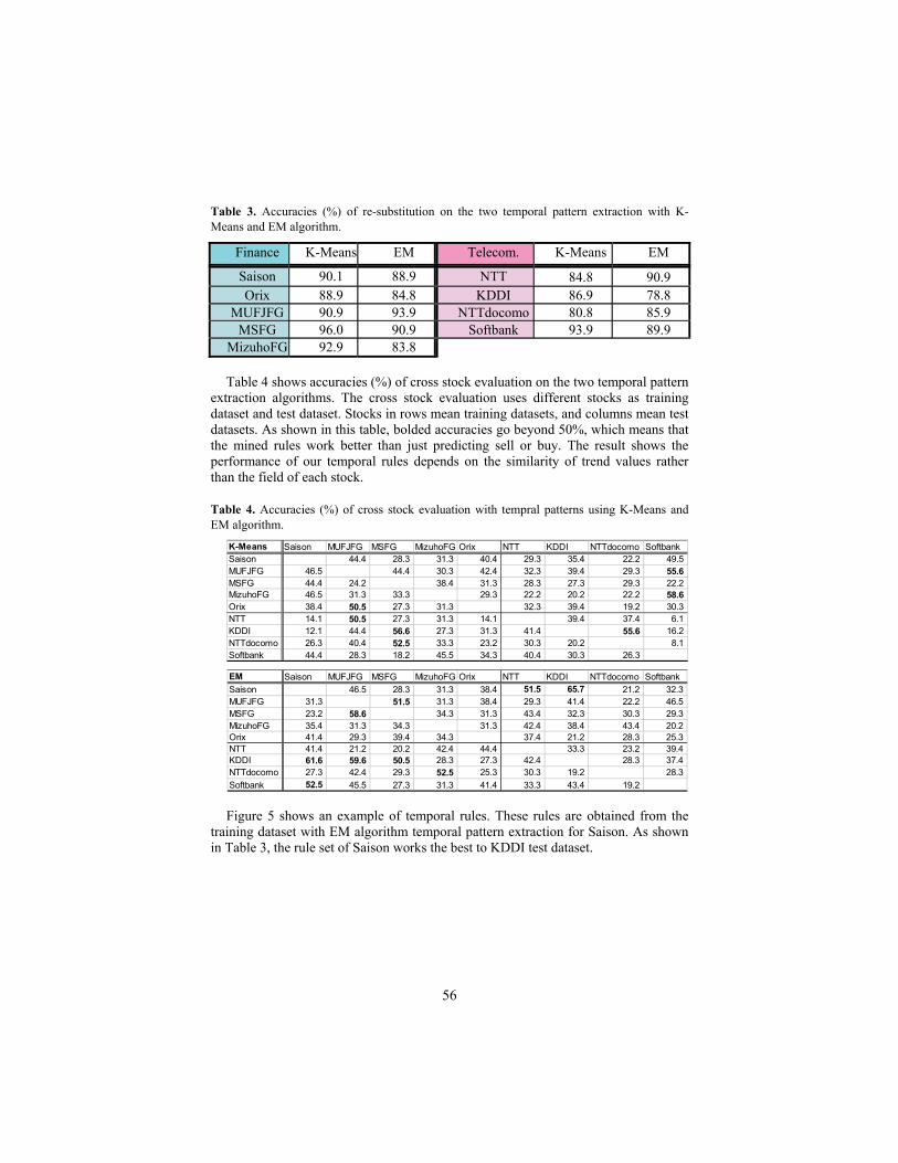
Table 3. Accuracies (%) of re-substitution on the two temporal pattern extraction with K-Means and EM algorithm.

Finance K-Means EM Telecom. K-Means EM

Saison 90.1 88.9 NTT 84.8 90.9 Orix 88.9 84.8 KDDI 86.9 78.8

MUFJFG 90.9 93.9 NTTdocomo 80.8 85.9 MSFG 96.0 90.9 Softbank 93.9 89.9

MizuhoFG 92.9 83.8 Table 4 shows accuracies (%) of cross stock evaluation on the two temporal pattern

extraction algorithms. The cross stock evaluation uses different stocks as training dataset and test dataset. Stocks in rows mean training datasets, and columns mean test datasets. As shown in this table, bolded accuracies go beyond 50%, which means that the mined rules work better than just predicting sell or buy. The result shows the performance of our temporal rules depends on the similarity of trend values rather than the field of each stock.

Table 4. Accuracies (%) of cross stock evaluation with tempral patterns using K-Means and EM algorithm.

K-Means Saison MUFJFG MSFG MizuhoFG Orix NTT KDDI NTTdocomo SoftbankSaison 44.4 28.3 31.3 40.4 29.3 35.4 22.2 49.5MUFJFG 46.5 44.4 30.3 42.4 32.3 39.4 29.3 55.6MSFG 44.4 24.2 38.4 31.3 28.3 27.3 29.3 22.2MizuhoFG 46.5 31.3 33.3 29.3 22.2 20.2 22.2 58.6Orix 38.4 50.5 27.3 31.3 32.3 39.4 19.2 30.3NTT 14.1 50.5 27.3 31.3 14.1 39.4 37.4 6.1KDDI 12.1 44.4 56.6 27.3 31.3 41.4 55.6 16.2NTTdocomo 26.3 40.4 52.5 33.3 23.2 30.3 20.2 8.1Softbank 44.4 28.3 18.2 45.5 34.3 40.4 30.3 26.3 EM Saison MUFJFG MSFG MizuhoFG Orix NTT KDDI NTTdocomo SoftbankSaison 46.5 28.3 31.3 38.4 51.5 65.7 21.2 32.3MUFJFG 31.3 51.5 31.3 38.4 29.3 41.4 22.2 46.5MSFG 23.2 58.6 34.3 31.3 43.4 32.3 30.3 29.3MizuhoFG 35.4 31.3 34.3 31.3 42.4 38.4 43.4 20.2Orix 41.4 29.3 39.4 34.3 37.4 21.2 28.3 25.3NTT 41.4 21.2 20.2 42.4 44.4 33.3 23.2 39.4KDDI 61.6 59.6 50.5 28.3 27.3 42.4 28.3 37.4NTTdocomo 27.3 42.4 29.3 52.5 25.3 30.3 19.2 28.3Softbank 52.5 45.5 27.3 31.3 41.4 33.3 43.4 19.2 Figure 5 shows an example of temporal rules. These rules are obtained from the

training dataset with EM algorithm temporal pattern extraction for Saison. As shown in Table 3, the rule set of Saison works the best to KDDI test dataset.

56

Fig. 5. An example of rule for 'buy' and rule for 'sell'.

0

0.5

1

-75 -65 -55 -45 -35 -25 -15 -5

opening

BolingerBand

M om entum

openingBolingerBand

momentum

5780

5610

sell

buy

186.2

-172.0

days

The rule for 'buy'The rule for 'buy'

0

0.5

1

-75 -65 -55 -45 -35 -25 -15 -5

Ichim oku4

Ichimoku4

buy

hold

days

The rule for ‘sell'The rule for ‘sell'

4.3 Discussion about the temporal rule mining

The prediction of decisions for each dataset works correctly with regarding to the result of Table 3, predicting temporal patterns of test dataset with a classification learning algorithm. However, mined rules based on temporal patterns are rather over fitting to each training dataset as shown in Table 4. One of the solutions to avoid over fitting will be to mine a temporal rule set from a training dataset, which consists of multiple stocks.

With regarding to Figure 5, our temporal rule mining system can find out adequate combinations of trend index patterns for each stock. To learn adequate trend index pattern combinations is very costly work for trading beginners. Thus, our temporal rule mining can support traders who want to know the adequate combinations of trend indices for each stock.

5 Conclusion

We have designed and implemented a temporal data mining environment, which integrates temporal pattern extraction, rule induction, and rule evaluation.

As the result of the case study on the nine Japanese stock datasets, this environment mines valuable temporal rules to predict different stock decisions based on temporal pattern extraction. The result also indicated the availability to support stock traders to learn adequate combinations of trend index patterns.

In future, we will evaluate trading result with the predictions of decisions by each mined temporal rule set on the stock trading simulator included in Kaburobo SDK.

Although we have not tried to select proper algorithms for the temporal pattern extraction procedure, the attribute selection procedure and the mining procedure, it is also able to connect subsystems for selecting each proper algorithm to this environment.

57

References

1. Berndt, D. J. and Clifford, J. “Using dynamic time wrapping to find patterns in time series”, in Proc. of AAAI Workshop on Knowledge Discovery in Databases (1994) pp.359-370

2. Das, G., King-Ip, L., Heikki, M., Renganathan, G., and Smyth, P., “Rule Discovery from Time Series”, in Proc. of International Conference on Knowledge Discovery and Data Mining (1998) pp.16-22

3. Fayyad, U. M., Piatetsky-Shapiro, G., and Smyth, P., “From Data Mining to Knowledge Discovery: An Overview”, Advances in Knowledge Discovery and Data Mining, AAAI Press / The MIT Press, CA (1996) pp.1-34

4. Frank, E., Witten, I. H., “Generating accurate rule sets without global optimization”, in Proc. of the Fifteenth International Conference on Machine Learning (1998) pp.144-151

5. Hirano, S. and Tsumoto, S., “Mining Similar Temporal Patterns in Long Time-Series Data and Its Application to Medicine”, in Proc. of the 2002 IEEE International Conference on Data Mining (2002) pp.219-226

6. Lin, J., Keogh, E., Lonardi, S., and Patel, P., “Finding Motifs in Time Series”, in Proc. of Workshop on Temporal Data Mining (2002) pp.53-68

7. Liu, H., and Motoda, H., “Feature selection for knowledge discovery and data mining”, Kluwer Academic Publishers (1998)

8. Michalski, R., Mozetic, I., Hong, J., and Lavrac, N., “The AQ15 Inductive Leaning System: An Overview and Experiments”, Reports of Machine Leaning and Inference Laboratory, MLI-86-6, George Maseon University, (1986)

9. Mitchell, T. M., “Generalization as Search”, Artificial Intelligence, 18(2) (1982) pp.203-226 10.Ohsaki, M., Sato, Y., Yokoi, H., and Yamaguchi T., "A Rule Discovery Support System for

Sequential Medical Data - In the Case Study of a Chronic Hepatitis Dataset -, ECML/PKDD-2003 Workshop on Discovery Challenge, (2003) pp.154-165

11. Ohsaki, M. Kitaguchi, S., Okamoto, K., Yokoi, H., and Yamaguchi, T., “Evaluation of Rule Interestingness Measures with a Clinical Dataset on Hepatitis”, in Proc. of ECML/PKDD 2004, LNAI3202 (2004) pp.362-373

12.Ohsaki, M., Abe, H., Kitaguchi, S., Kume, S., Yokoi, H., and Yamaguchi, T., “Development and Evaluation of an Integrated Time-Series KDD Environment - A Case Study of Medical KDD on Hepatitis-", Joint Workshop of Vietnamese Society of Artificial Intelligence, SIGKBS-JSAI, ICS-IPSJ and IEICE-SIGAI on Active Mining (2004) No.23.

13. Quinlan, J. R., “Programs for Machine Learning”, Morgan Kaufmann (1992) 14.Quinlan, J. R., "Bagging, Boosting and C4.5", AAAI/IAAI, 1 (1996) pp. 725-730 15. Raymond, W., and Ada, F., "Mining top-K frequent itemsets from data streams", Data

Mining and Knowledge Discovery, 13(2) (2006) pp.193-217 16. Witten, I. H. and Frank, E., “Data Mining: Practical Machine Learning Tools and

Techniques with Java Implementations”, Morgan Kaufmann, San Francisco (2000) 17. KabuRobo: [http://www.kaburobo.jp] (in Japanese)

58

Discriminant Feature Analysis for Music Timbre Recognition

Xin Zhang1, Zbigniew W. Ras1,2

1 Computer Science Department, University of North Carolina, Charlotte, N.C., USA,

2 Polish-Japanese Institute of Information Technology, 02-008 Warsaw, Poland {xinzhang, ras}@uncc.edu

Abstract. The high volume of digital music recordings in the internet repositories has brought a tremendous need for automatic recommendation system based on content data to help users to find their favorite music items. Music instrument identification is one of the important subtasks of content-based automatic indexing, for which the authors have developed novel new temporal features and implemented a high dimensional sound feature database with all the low-level MPEG7 descriptors as well as popular features in the literature. This paper presents development details of these new features and evaluates them among other 300 features in the database by a logistic discriminant analysis for improving music instrument identification efficiency of rule-based classifiers.

Keywords: Automatic Indexing, Music Information Retrieval, MPEG7, Timbre Estimation, Logistic Discriminant Analysis, Feature Selection, and Machine Learning.

1 Introduction

The state of art technologies in network and computer storage boost the fast growing of music repositories throughout the Internet, which brought the need for music intelligence techniques to help users to find their favorite music items.

Aiming to provide efficient music recommendations, data mining of different representations of musical files (e.g., music recording, MIDI file, and music notes) involves very different techniques respectively: research in MIDI files and music notes tackles problems in text mining, where intuitively Music Information Retrieval (MIR) needs not to be considered; knowledge discovery in digital recordings requires MIR of sound features from musical sound signals, since digital recordings contain only sound signals unless manually labeled with semantic descriptions (e.g., author, title, and company). Timbre identification is one of the important subtasks for mining digital recordings, where timbre is a quality of sound that distinguishes one music instrument

59

from another. Researchers in this area have investigated a number of acoustical features to build computational model for timbre identification. In this paper, authors focus on developing automated indexing solutions for digital recordings based on MIR techniques of instruments and their types.

The real use of timbre-based grouping of music is very nicely discussed in [3]. Methods in research on automatic musical instrument sound classification go back to last few years. Next, the paper reviews these algorithms in two categories: monophonic and polyphonic, which are defined by the total instruments within the target sounds.

For monophonic sounds, a number of acoustic features have been explored by researchers in this field ([1] and [4]). Some of them are quite successful on certain simple sound data (monophonic, short, of limited instrument types). The challenges for instrument identification in this type of sounds are at least in these areas: a digital multimedia file normally contains a huge amount of data, where subtle changes of sound amplitude in time can be critical for human perception system, thus the data-driven timbre identification process demands lots of information to capture and describes the patterns among those subtle changes; since after the dimensional approach to timbre description was proposed by [3], so far there is no standard parameterization used as a classification basis. Researchers in the area have been explored different statistical parameters to describe patterns and properties of the spectrums of music sounds to distinguish different timbre, such as Tristimulus parameters [10], brightness [5], and irregularity [16], etc. Based on recent research performed in this area, MPEG-7 standard provides a set of low-level temporal and spectral sound features where some of them are in a form of vector or matrix of a large size. Flattening and summarizing these features for traditional classifiers intuitively increases the number of features and losses some potentially useful information. Therefore, in this paper, authors are proposing new features which are sufficient in musical timbre signatures and suitable in format for machine learning classifiers. Authors compare them against popular features in the literature to improve the classification efficiency by logistic regression studies.

For polyphonic sounds, different methods have been investigated by various researchers and mathematicians, such as Independent Component Analysis (ICA) ([6] and [15]), Factorial Hidden Markov Models (HMM) ([9] and [13]), and Harmonic Sources Separation Algorithms ([2], [18], [7], and [20]). ICA requires multiple channels of different sound sources. Most often, HMM works well for sound sources separation, where fundamental frequency range is small and the variation is subtle. Harmonic Sources Separation Algorithms can be used to isolate sound sources within a single channel, where efficient solution in one channel can be intuitively applied to other channels and therefore facilitates more types of sound recordings (e.g., mono-channel and stereo with two or more channels). The authors also have interest to apply the proposed features to their harmonic sound source isolation system [18] in order to improve its isolation accuracy.

60

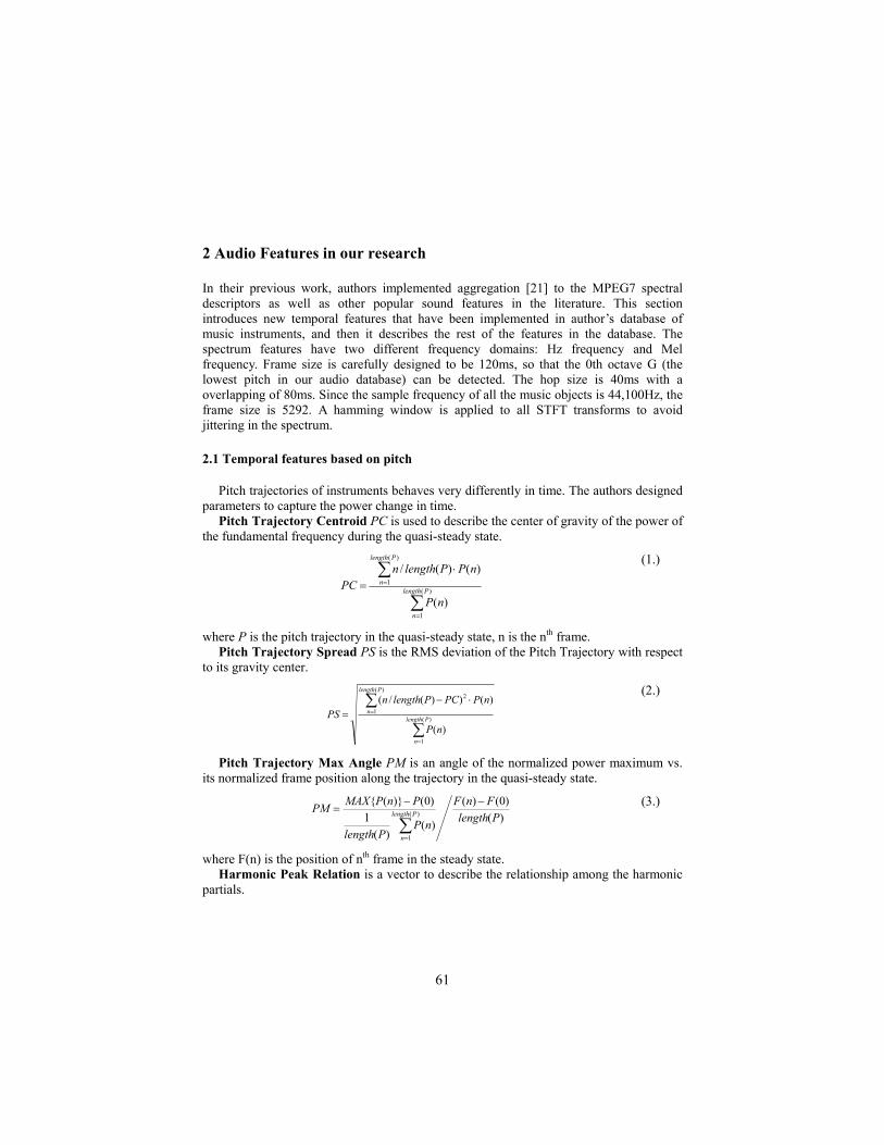
2 Audio Features in our research

In their previous work, authors implemented aggregation [21] to the MPEG7 spectral descriptors as well as other popular sound features in the literature. This section introduces new temporal features that have been implemented in author’s database of music instruments, and then it describes the rest of the features in the database. The spectrum features have two different frequency domains: Hz frequency and Mel frequency. Frame size is carefully designed to be 120ms, so that the 0th octave G (the lowest pitch in our audio database) can be detected. The hop size is 40ms with a overlapping of 80ms. Since the sample frequency of all the music objects is 44,100Hz, the frame size is 5292. A hamming window is applied to all STFT transforms to avoid jittering in the spectrum.

2.1 Temporal features based on pitch

Pitch trajectories of instruments behaves very differently in time. The authors designed parameters to capture the power change in time.

Pitch Trajectory Centroid PC is used to describe the center of gravity of the power of the fundamental frequency during the quasi-steady state.

∑

∑

=

=

⋅= )(

1

)(

1

)(

)()(/

Plength

n

Plength

n

nP

nPPlengthnPC

(1.)

where P is the pitch trajectory in the quasi-steady state, n is the nth frame. Pitch Trajectory Spread PS is the RMS deviation of the Pitch Trajectory with respect

to its gravity center.

∑

∑

=

=

⋅−= )(

1

)(

1

2

)(

)())(/(

Plength

n

Plength

n

nP

nPPCPlengthnPS

(2.)

Pitch Trajectory Max Angle PM is an angle of the normalized power maximum vs. its normalized frame position along the trajectory in the quasi-steady state.

)()0()(

)()(

1)0()}({

)(

1

PlengthFnF

nPPlength

PnPMAXPM Plength

n

−−=

∑=

(3.)

where F(n) is the position of nth frame in the steady state. Harmonic Peak Relation is a vector to describe the relationship among the harmonic

partials.

61

01

/1 HHm

HRm

ij∑

=

= (4.)

where m is the total number of frames in the steady state, Hj is the jth harmonic peak in the ith frame.

2.2 Aggregation features

MPEG7 descriptors can be categorized into two types: temporal and spectral. The authors applied aggregation among all the frames per music object for all the following instantaneous spectral features.

MPEG7 Spectrum Centroid [22] describes the center-of-gravity of a log-frequency power spectrum. It economically indicates the pre-dominant frequency range. Coefficients under 62.5Hz have been grouped together for fast computation.

MPEG7 Spectrum Spread is the Root of Mean Square value of the deviation of the Log frequency power spectrum with respect to the gravity center in a frame [22]. Like Spectrum Centroid, it is an economic way to describe the shape of the power spectrum.

MPEG7 Harmonic Centroid is computed as the average over the sound segment duration of the instantaneous Harmonic Centroid within a frame [22]. The instantaneous Harmonic Spectral Centroid is computed as the amplitude in linear scale weighted mean of the harmonic peak of the spectrum.

MPEG7 Harmonic Spread is computed as the average over the sound segment duration of the instantaneous harmonic spectral spread of frame [22]. The instantaneous harmonic spectral spread is computed as the amplitude weighted standard deviation of the harmonic peaks of the spectrum with respect to the instantaneous harmonic spectral centroid.

MPEG7 Harmonic Variation is defined as the mean value over the sound segment duration of the instantaneous harmonic spectral variation [22]. The instantaneous harmonic spectral variation is defined as the normalized correlation between the amplitude of the harmonic peaks of two adjacent frames.

MPEG7 Harmonic Deviation is computed as the average over the sound segment duration of the instantaneous Harmonic Spectral Deviation in each frame [22]. The instantaneous Harmonic Spectral Deviation is computed as the spectral deviation of the log amplitude components from a spectral envelope.

MPEG7 Harmonicity Rate is the proportion of harmonics in the power spectrum. It describes the degree of harmonicity of a frame [22]. It is computed by the normalized correlation between the signal and a lagged representation of the signal.

MPEG7 Fundamental Frequency is the frequency that best explains the periodicity of a signal [22]. The ANSI definition of psycho-acoustical terminology says that “pitch is an auditory attribute of a sound according to which sounds can be ordered on a scale from low to high”.

62

MPEG7 Upper Limit of Harmonicity describes the frequency beyond which the spectrum cannot be considered harmonic [22]. It is calculated based on the power spectrum of the original and a comb-filtered signal.

Tristimulus and similar parameters describe the ratio of the amplitude of a harmonic partial to the total harmonic partials [10]. They are first modified tristimulus parameter, power difference of the first and the second tristimulus parameter, grouped tristimulus of other harmonic partials, odd and even tristimulus parameters.

∑=

=N

nnAATr

1

2211

(5.)

∑∑==

=N

jj

ii AAh

1

24

3

24,3

(6.)

∑∑==

=N

jj

ii AAh

1

27

5

27,6,5

(7.)

∑∑==

=N

jj

ii AAh

1

210

8

210,9,8

(8.)

∑∑==

−=N

nn

L

kk AAOd

1

2

2

212

(9.)

∑∑==

=N

nn

M

kk AAEv

1

2

1

22

(10.)

∑∑==

Δ=5

11

5

1/))/((

kkk

kkm AfkfAfd

(11.)

Brightness is calculated as the proportion of the weighted harmonic partials to the harmonic spectrum [5].

∑∑==

⋅=N

nn

N

nn AAnB

11

(12.)

Transient, steady and decay duration in this research, the transient duration is considered as the time to reach the quasi-steady state of fundamental frequency. In this duration the sound contains more timbre information than pitch information that is highly relevant to the fundamental frequency. Thus differentiated harmonic descriptors values in time are calculated based on the subtle change of the fundamental frequency [19].

Zero crossing counts the number of times that the signal sample data changes signs in a frame [12] [14].

63

∑=

−−=N

niii nssignnssignZC

1])1[(])[(5.0 (13.)

⎩⎨⎧

<−≥

=0,1

0,1)(

xx

xsign (14.)

where Si is the nth sample in the ith frame, N is the frame size. Spectrum Centroid describes the gravity center of the spectrum [12] [17]

∑

∑

=

== 2/

1

2/

1

)(

)()(

N

ki

N

ki

i

kX

kXkfC

(15.)

where N is the total number of the FFT points, Xi(k) is the power of the kth FFT point in the ith frame, f(k) is the corresponding frequency of the FFT point.

Roll-off is a measure of spectral shape, which is used to distinguish between voiced and unvoiced speech [8]. The roll-off is defined as the frequency below which C percentage of the accumulated magnitudes of the spectrum is concentrated, where C is an empirical coefficient.

∑∑==

⋅≤K

ki

K

ki kXCkX

11)()( (16.)

Flux is used to describe the spectral rate of change [12]. It is computed by the total difference between the magnitude of the FFT points in a frame and its successive frame.

( )∑=

−−=2/

1

21 )()(

N

kiii kXkXF (17.)

2.3 Statistical parameters

Also, to flatten the matrix data to suitable format for the classifiers, statistical parameters (e.g., maximum, minimum, average, distance of similarity, standard deviation) are applied to the power of each spectral band.

MPEG7 Spectrum Flatness describes the flatness property of the power spectrum within a frequency bin, which is ranged by edges in the following formula [22]. The value of each bin is treated as an attribute value in the database. Since the octave resolution in our research is 1/4, the total number of bands is 32.

MPEG7 Spectrum Basis Functions Vk are used to reduce the dimensionality by projecting the spectrum from high dimensional space to low dimensional space with compact salient statistical information [22]. tx is a vector of power spectrum coefficients

64

in a frame t, which are transformed to Db scale and then normalized. N, the total number of frequency bins, is 32 in 1/4 octave resolution.

Mel frequency cepstral coefficients describes the spectrum according to the human perception system in the mel scale. They are computed by grouping the STFT points of each frame into a set of 40 coefficients by a set of 40 weighting curves with logarithmic transform and a discrete cosine transform (DCT).

2.4 MPEG7 temporal descriptors

The temporal descriptors in MPEG7 [22] have been applied directly into the feature database. MPEG7 Spectral Centroid is computed as the power weighted average of the frequency bins in the power spectrum of all frames in a sound segment with a Welch method. MPEG7 Log Attack Time is defined as the logarithm of the time duration between the time when the signal starts to the time it reaches its stable part, where the signal envelope is estimated by computing the local mean square value of the signal amplitude in each frame. MPEG7 Temporal Centroid is calculated as the time average over the energy envelope.

3 Discriminant Analysis for Feature Selection

Logistic regression model is a popular statistical approach of analyzing multinomial response variables, since it does not assume normally distributed conditional attributes which can be continuous, discrete, dichotomous or a mix of any of these; it can handle nonlinear relationships between the discrete responses and the explanatory attributes. It has been widely used to investigate the relationship between decision attribute and conditional attributes, using the most economical model. An ordinal response logit model has a form:

,)|1Pr(

)|Pr(log xxkY

xiYii βα +=⎟⎟

⎠

⎞⎜⎜⎝

⎛+=

= , i=1,…k (18.)

where the k+1 possible responses have no natural ordering and α1, …, αk are k intercept parameters, β1, …, βk are k vectors of parameters, and Y is the response. For details, see [11]. The system fits a common slopes cumulative model which is a parallel lines regression model based on the cumulative probabilities of the response categories. The significance of an attribute is calculated with the likelihood ratio or chi-square difference test by the Fisher’s Score algorithm. A final model is selected, where adding another variable would not improve the model significantly.

65

4 Experiments

The authors implemented a feature database of 1569 music recording sound objects of 74 instruments, which can play music notes, from McGill University Master Samples CD collection, which has been widely used for research on musical instrument recognition all over the world. The authors discriminated instrument types on different levels of a classification tree. The tree consists of three levels: the top level (e.g., aerophone, chordophone, and idiophone), the second level (e.g., lip-vibrated, side, reed, composite, simple, rubbed, shaken, and struck), and the third level (e.g., piano, violin, and flute.). All classifiers were 10-fold cross validation with a split of 90% training and 10% testing. We used WEKA for all classifications and SAS LOGISTIC procedure for discriminant analysis. In each experiment, a 99% confidence level is used. Feature extraction was implemented in .NET C++ with connection to MS SQL Server.

Figure 1. Music instrument classification tree.

For classification on the first level in the music instrument family tree, the selected

feature set was stored in List I: { PeakRelation8, PeakRelation16, PeakRelation24, MPEGFundFreq, MPEGHarmonicRate, MPEGULHarmonicity, MPEGHarmoVariation, MPEGHarmoDeviation, MPEGFlat3, MPEGFlat8, MPEGFlat18, MPEGFlat30, MPEGFlat36, MPEGFlat46, MPEGFlat55, MPEGFlat56, MPEGFlat66, MPEGFlat67, MPEGFlat76, MPEGFlat77, MPEGFlat83, MPEGFlat85, MPEGFlat94, MPEGFlat96, MPEGSpectrumCentroid, MPEGTC, MPEGBasis59, MPEGBasis200, TristimulusRest, ZeroCrossing, MFCCMaxBand1, MFCCMaxBand3, MFCCMaxBand5, MFCCMaxBand6, MFCCMaxBand7, MFCCMaxBand8, MFCCMaxBand10, MFCCMaxBand13, MFCCMinBand1, MFCCMinBand13, PitchSpread, MaxAngle}. Experiment was also performed on the rest of features after List I was removed from the whole feature set, which was stored in List II. In the table below, “All” stands for all the attributes used for classifier construction.

66

Table 1. Results of three groups of features at the top level of the music family tree.

Precision Recall

List I All List II List I All List II Idiophone 87.00% 91.10% 95.10% 82.10% 91.40% 94.80%

Chordophone 86.80% 91.30% 88.50% 88.60% 88.90% 84.70% Aerophone 91.50% 91.30% 87.30% 91.80% 93.50% 90.90%

Table1 shows the precisions of the classifiers constructed with selected features at the

family level. After the less significant features, elected by the logistic model, have been removed, the group of List I slightly improved the precision for aerophone instruments. However, the selected significant feature group (List I) significantly outperformed in precision for aerophone instruments and in recall for both chordophone and aerophone instruments.

For classification at the second level in the music instrument family tree, the selected feature set was stored in List I: {PeakRelation8, PeakRelation16, PeakRelation30, MPEGFundFreq, MPEGHarmonicRate, MPEGULHarmonicity, MPEGHarmoDeviation, MPEGFlat3, MPEGFlat11, MPEGFlat14, MPEGFlat18, MPEGFlat22, MPEGFlat26, MPEGFlat36, MPEGFlat44, MPEGFlat46, MPEGFlat58, MPEGFlat67, MPEGFlat81, MPEGFlat82, MPEGFlat83, MPEGFlat85, MPEGFlat93, MPEGFlat94, MPEGFlat95, MPEGSpectrumCentroid, MPEGTC, MPEGBasis50, MPEGBasis57, MPEGBasis59, MPEGBasis69, MPEGBasis73, MPEGBasis116, MPEGBasis167, MPEGBasis206, Tristimulus1, TristimulusRest, TristimulusBright, ZeroCrossing, SpectrumCentroid2, RollOff, MFCCMaxBand1, MFCCMaxBand3, MFCCMaxBand4, MFCCMaxBand6, MFCCMaxBand7, MFCCMaxBand9, MFCCMinBand2, MFCCMinBand5, MFCCMinBand10, MFCCMinBand13, MFCCAvgBand10, MFCCAvgBand11, PitchSpread, MaxAngle}. Experiment was also performed on List II obtained by removing List I from the whole feature set.

Table 2. Results of three groups of features at the second level of the music family tree.

Precision Recall

List I All List II List I All List II Lip-Vibrated 83.80% 84.40% 77.30% 84.70% 88.80% 82.30% Side 74.30% 73.20% 66.40% 75.70% 64.00% 64.00% Reed 77.10% 78.30% 70.50% 78.40% 80.10% 70.50% Composite 84.50% 86.20% 84.90% 86.70% 84.30% 83.90% Simple 71.20% 74.10% 72.20% 67.20% 80.00% 72.80% Rubbed 85.30% 82.10% 75.00% 78.40% 86.50% 73.00% Shaken 79.20% 91.00% 89.50% 64.80% 92.00% 87.50% Struck 78.20% 86.30% 85.40% 80.40% 79.00% 77.60% Table2 shows the precisions of the classifiers constructed with the selected features, all

features, and the rest of the features after selection at the second level of the instrument

67

family tree. After the less significant features, elected by the logistic model, have been removed, the group of List I improved the precision for side and rubbed instruments and recall for the side, composite, and struck instruments. Also, the selected significant feature group (List I) significantly outperformed in precision for lip-vibrated, side, reed, and rubbed instruments and in recall for all the types except for simple and shaken instruments.

For classification at the third level in the music instrument family tree, the selected feature set was stored in List I: { MPEGTristimulusOdd, MPEGFundFreq, MPEGULHarmonicity, MPEGHarmoVariation, MPEGFlatness6, MPEGFlatness14, MPEGFlatness27, MPEGFlatness35, MPEGFlatness43, MPEGFlatness52, MPEGFlatness63, MPEGFlatness65, MPEGFlatness66, MPEGFlatness75, MPEGFlatness76, MPEGFlatness79, MPEGFlatness90, MPEGFlatness91, MPEGSpectrumCentroid, MPEGSpectrumSpread, MPEGBasis41, MPEGBasis42, MPEGBasis69, MPEGBasis87, MPEGBasis138, MPEGBasis157, MPEGBasis160, MPEGBasis170, MPEGBasis195, TristimulusBright, TristimulusEven, TristimulusMaxFd, ZeroCrossing, SpectrumCentroid2, Flux, MFCCMaxBand2, MFCCMaxBand3, MFCCMaxBand6, MFCCMaxBand7, MFCCMaxBand9, MFCCMaxBand10, MFCCMinBand1, MFCCMinBand2, MFCCMinBand3, MFCCMinBand6, MFCCMinBand7, MFCCMinBand10, MFCCAvgBand1, MFCCAvgBand12, SteadyEnd, Length}. Experiment was also performed on List II obtained by removing List I from the whole feature set.

Table 3. Results of three groups of features at the third level of the music family tree.

Precision Recall

List I All List I All List I All flute 92.90% 67.70% 70.40% 89.70% 72.40% 65.50%

tubularbells 86.70% 60.00% 52.40% 72.20% 66.70% 61.10% tuba 85.70% 81.80% 85.70% 90.00% 90.00% 90.00%

electricbass 83.10% 87.50% 89.10% 80.60% 83.60% 85.10% Trombone 80.60% 80.00% 76.30% 69.20% 82.10% 74.40% marimba 79.20% 89.50% 90.60% 71.40% 89.50% 86.50%

piano 78.50% 82.40% 83.00% 81.60% 78.40% 74.40% frenchhorn 78.00% 83.70% 82.90% 87.70% 88.90% 84.00% bassflute 77.40% 75.50% 71.20% 68.30% 61.70% 61.70% altoFlute 76.70% 82.80% 78.60% 79.30% 82.80% 75.90%

doublebass 75.40% 60.80% 60.00% 75.40% 54.40% 52.60% piccolo 74.50% 69.20% 62.00% 71.70% 67.90% 58.50%

ctrumpet 72.00% 68.90% 69.10% 83.10% 78.50% 72.30% violin 71.00% 75.00% 77.10% 78.00% 72.70% 76.50% oboe 70.30% 71.00% 35.90% 81.30% 68.80% 43.80%

vibraphone 69.30% 91.40% 85.70% 73.20% 90.10% 93.00% bassoont 68.80% 66.70% 45.50% 61.10% 55.60% 27.80%

cello 67.00% 63.20% 63.50% 61.50% 62.50% 68.80% saxophone 66.70% 51.70% 53.60% 46.70% 50.00% 50.00%

68

Table3 shows statistics of the precisions of the classifiers constructed with the selected

features, all features, and the rest of the features after selection in the bottom level of the family tree for some instruments in the experiment. The overall accuracy of all the features was slightly better than that of the selected features. The computing time for List I, All, and List II is 7.33, 61.59, and 54.31 seconds respectively.

5 Conclusion and future work

A large number of attributes is generated in a table during fattening the features into a single value attributes for classical classifiers by statistical and other feature design methods. Some of the derived attributes may not significantly contribute to the classification models, or sometimes may distract the classification. In the light of the results from the experiments, we conclude that attributes have different degree of influence on the classification performance for different instrument families. The new temporal features related to harmonic peaks significantly improved the classification performance when added into the database with all other features. However, the new features were not suitable to replace the MPEG7 harmonic peak related features and Tristimulus parameters as the logistic studies shows. We also noticed that classifications at a higher level of granularity tended to use more features for correct prediction than those at the lower level. This may especially benefit a cooperative query answering system to choose suitable features for classifiers at different levels.

Acknowledgments. This work is supported by the National Science Foundation under grant IIS-0414815.

6 References

[1] Balzano, G.J. (1986). What are musical pitch and timbre? Music Perception - an interdisciplinary Journal, 3, pp. 297-314.

[2] Bay, M. and Beauchamp, J.W. (2006). Harmonic source separation using prestored spectra, ICA 2006, LNCS 3889, pp. 561 – 568, 2006.

[3] Bregman, A.S. (1990). Auditory scene analysis, the perceptual organization of sound, MIT Press.

[4] Cadoz, C. (1985). Timbre et causalite, Unpublished paper, Seminar on Timbre, Institute de Recherche et Coordination Acoustique / Musique, Paris, France, April 13-17.

[5] Fujinaga, I., McMillan, K. (2000) Real time Recognition of Orchestral Instruments, International Computer Music Conference, pp. 141-143.

[6] Kinoshita, T., Sakai, S., and Tanaka, H. (1999). Musical sound source identification based on frequency component adaptation, in Proceedings of IJCAI Workshop on Computational Auditory Scene Analysis (IJCAI-CASA '99), Stockholm, Sweden, July-August, pp. 18–24.

69

[7] Kitahara,T., Goto, M., Komatani, K., Ogata, T., and Okuno, H.G. (2007)Instrument Identification in PolyphonicMusic: Feature Weighting toMinimize Influence of Sound Overlaps.EURASIP Journal on Advances in Signal Processing, Volume 2007, Article ID 51979.

[8] Lindsay, A. T., and Herre, J. (2001) MPEG-7 and MPEG-7 Audio—An Overview, J. Audio Eng. Soc., vol.49, July/Aug, pp. 589–594.

[9] Ozerov,A., Philippe, P., Gribonval, R., and Bimbot, F. (2005) One microphone singing voice separation using source adapted models, in Proc. IEEE Workshop on Applications of Signal Processing to Audio and Acoustics (WASPAA), pp. 90-93.

[10] Pollard, H.F. and Jansson, E.V. (1982). A tristimulus Method for the specification of Musical Timbre. Acustica, 51, pp. 162-171

[11] Cessie, S. le and Houwelingen, J.C.(1992).Ridge Estimators in Logistic Regression, Applied Statistics, vol. 41, no. 1, pp. 191-201.

[12] Scheirer, E. and Slaney, M. (1997). Construction and Evaluation of a Robust Multi-feature Speech/Music Discriminator, in Proc. IEEE int. Conf. on Acoustics, Speech and Signal Processing (ICASSP).

[13] Smith, J.O. and Serra, X. (1987). PARSHL: An Analysis/Synthesis Program for Non Harmonic Sounds Based on a Sinusoidal Representation. In Proc. Int. Computer Music Conf., Urbana-Champaign, Illinois, pp.290-297.

[14] Tzanetakis, G. and Cook, P. (2002). Musical Genre Classification of Audio Signals, IEEE Trans. Speech and Audio Processing, July, vol. 10, pp. 293–302.

[15] Vincent, E. (2006). Musical source separation using time-frequency source priors, IEEE Transactions on Audio, Speech and Language Processing, vol. 14, no. 1, pp. 91–98.

[16] Wieczorkowska, A. (1999). Classification of musical instrument sounds using decision trees, in the 8th International Symposium on Sound Engineering and Mastering, ISSEM'99, pp. 225-230.

[17] Wold, E., Blum, T., Keislar, D., and Wheaton, J,(1996). Content-Based Classification, Search and Retrieval of Audio, IEEE Multimedia,Fall, pp. 27–36.

[18] Zhang, X., Marasek, K. and Ras, Z. W. (2007). Maximum Likelihood Study for Sound Pattern Separation and Recognition. In Proceedings of the IEEE CS International Conference on Multimedia and Ubiquitous Engineering (MUE 2007). April 26–28, Seoul, Korea, pp. 807-812.

[19] Zhang, X. and Ras, Z.W. (2006). Differentiated Harmonic Feature Analysis on Music Information Retrieval For Instrument Recognition, proceeding of IEEE International Conference on Granular Computing, May 10-12, Atlanta, Georgia, pp. 578-581.

[20] Zhang, X. and Ras, Z.W. (2006). Sound Isolation by Harmonic Peak Partition For Music Instrument Recognition, Fundamenta Informaticae Journal Special issue on Tilings and Cellular Automata, IOS Press, pp. 612-628.

[21] Zhang, X. and Ras, Z.W. (2007). Analysis of Sound Features for Music Timbre Recognition. Invited paper. In Proceedings of the IEEE CS International Conference on Multimedia and Ubiquitous Engineering (MUE 2007). April 26–28, Seoul, Korea, pp. 3-8. [22] ISO/IEC JTC1/SC29/WG11 (2002). MPEG-7 Overview. http://mpeg.telecomitalialab.com/standards/mpeg-7/mpeg-7.htm

70

Discovery of frequent graph patterns that consistof the vertices with the complex structures

Tsubasa Yamamoto1, Tomonobu Ozaki2 and Takenao Okawa1

1 Graduate School of Engineering, Kobe University2 Organization of Advanced Science and Technology, Kobe University

1-1 Rokkodai, Nada, Kobe 657-8501, JAPAN{yamamoto@cs25.scitec., tozaki@cs., ohkawa@}kobe-u.ac.jp

Abstract. In some applications, the data can be represented naturallyin a special kind of graphs that consist of vertices holding a set of (struc-tured) data such as item sets, sequences and so on. One of the typicalexamples is metabolic pathway. Metabolic pathway is represented in agraph structured data in which each vertex corresponds to an enzymedescribed by a set of various kinds of properties such as amino acidsequence, label and so on. We call this kind of complex graphs multi-structured graphs. In this paper, we propose an algorithm named FMGfor mining frequent patterns in multi-structured graphs. In FMG, theexternal structure will be expanded by general graph mining algorithm,while the internal structure will be enumerated by some algorithm suit-able for its structure. In addition, a pruning technique is introducedto exclude uninteresting patterns. The preliminary experimental resultswith real data show the effectiveness of the proposed algorithm.

1 Introduction

Graphs are widely used to represent complicated structures such as proteins, LSIcircuits, hyperlinks in WWW, XML data and so on. Discovering frequent sub-graphs from a graph database is one of the most important problems of the graphmining[3]. In recent years, several efficient algorithms of graph mining have beendeveloped[1, 6, 9, 10]. However, since the structure of data is becoming complexmore and more, these algorithms might not be sufficient in some applicationdomains. One typical example of such complex database is KEGG? , which is adatabase of metabolic pathways. Metabolism denotes total chemical reactions inthe body of organisms. The chemical reaction is risen up by some enzyme andit translates a compound into another compound. Pathway is the large networkof these reactions, so it can be regarded as a graph structured data. In addition,the vertices in the pathway consist of several types of data such as compounds,enzymes, genes and so on. Therefore, a metabolic pathway can be naturally rep-resented in a graph that consist of vertices holding a set of (structured) datasuch as item sets, sequences and so on. Since most of graph mining algorithms

? http://www.genome.ad.jp/kegg/

71

consider the element of vertices as an item, they can not discover frequent sub-graphs in which sub-patterns of vertex elements are considered. Because suchkind of complex graph data is expected to be going to rapidly increase, it isimportant to establish a flexible technique that can inclusively treat such kindof data.

In this paper, as one of the techniques to deal with such kind of complexgraphs, we propose a new frequent graph mining algorithm named FMG. Whilewe describe it in detail later, the target of FMG is special kind of graphs, calledmulti-structured graphs, that consist of vertices holding a set of (structured) datasuch as item sets, sequences and so on. Given a database of multi-structuredgraphs, FMG will discover frequent graph patterns that consist of vertices withseveral complex structures. In order to enumerate frequent patterns completely,while the external structures will be expanded in the manner of general graphmining algorithm, the internal structures, i.e. vertices, will be enumerated bysome algorithm suitable for those structures. In addition, FMG employs severalnovel optimization techniques to exclude uninteresting patterns.

The rest of this paper is organized as follows. In section 2, we introduce somebasic notations and define our data mining problem. In section 3, our frequentpattern miner FMG is proposed. Preliminary experimental results with pathwaysin KEGG are reported in section 4. After describing related work in section 5,we conclude this paper in section 6.

2 Preliminaries

A multi-structured graph G consists of a set of vertices V (G) and a set of edgesE(G). Each vertex v ∈ V (G) consists of a length n list of attributes of pluralkinds of structured data. We denote the list of v as list(v) = [elmv

1, · · · , elmvn] ∈

[dom(A1), · · · , dom(An)] where dom(Ai) denotes the domain of structure of ithattribute Ai. We show an example of multi-structured graph in Fig. 1. For ex-ample, for v13 ∈ V (G1), list(v13) is [{a, b, c}, 〈AACC〉] and the domain of thefirst and second attributes are item sets and sequences, respectively. A spanningtree of a graph is considered with depth first search for numbering the vertices.The first visited vertex is called root, while the last visited vertex is called right-most vertex. The path from the root to the rightmost vertex in the spanningtree is called rightmost path. In G1, if we set v11 to the root, then the rightmostvertex is v14 and the rightmost path becomes v11-v13-v14. We denote the edgeeij ∈ E(G) between ith and jth vertices. Edge labels are not considered in thispaper.

For example, from an attribute whose domain is graph, we can extract severalclasses of pattern, such as paths, trees and graphs. So, as a bias, we have togive the class of pattern PAi

to be extracted from each attribute Ai. Giventwo patterns p, q ∈ PAi , p ¹ q denotes that p is more general than or equalsto q. Given a vertex v with list(v) = [elmv

1, · · · , elmvn] and a list of patterns

lp = [p1, · · · , pn] ∈ [PA1 , · · · ,PAn ], if all pi cover its corresponding elmvi , then

we say that P covers v and denote it as lp ≺ v. Note that, we assume that each

72

combination of PAi and dom(Ai) gives the definitions of the cover relation andthe generality relation.

For two multi-structured graphs G and G′, a subgraph isomorphism, de-noted as G ⊆ G′, is an injective function f : V (G) ⇒ V (G′) such that (1)∀v ∈V (G) v ≺ f(v), and (2)∀eij ∈ E(G) f(eij) ∈ E(G′). If there exists a subgraphisomorphism from G to G′, G is called subgraph of G′ and G′ is called a su-pergraph of G. Let D = {G1, G2, · · · , GM} be a database of multi-structuredgraphs. The support of a multi-structured subgraph pattern P , hereafter graphpattern in short, is defined as follows.

supD(P ) =∑

G∈D OP (G)M

where OP (G) ={

1 (P ⊆ G)0 (otherwise)

Given a user defined threshold σ, a graph pattern P is called frequent in D ifsupD(P ) ≥ σ holds. The problem discussed in this paper is stated formally asfollows : Given a database D of multi-structured graphs and a positive numberσ(0 < σ ≤ 1) called the minimum support, find all frequent graph patterns Psuch that supD(P ) ≥ σ.

3 Mining Frequent Multi-structured Subgraph Patterns

In this section, we propose a frequent multi-structured subgraph pattern minernamed FMG. Throughout this section, we use the database shown in Fig. 1 asa running example for explaining the behavior of FMG.[ { a , b , c } , φ ][ φ ,

〈 B A C 〉] [ { a , b , c } ,〈 A A C C 〉 ][ { a , c , d } ,

〈 B A C 〉 ]G1

[ { b , c } ,〈 A A C C 〉 ][ { b , c , d } ,〈B A C C 〉][ { c } ,〈B C C 〉 ] [ φ ,

〈 A B C C 〉 ]v11

v12

v13

v14

G2

v21

v22

v23

v24

Fig. 1. Target database

FMG employs a kind of the pattern-growth approach [7, 9]. Initial patternsfor FMG are multi-structured graphs with one vertex. That is to say, they arethe set of all sub-patterns of the vertex element whose size is 1. For example,initial patterns taken from G1 are {a}, {b}, {c}, {d}, 〈A〉, 〈B〉 and 〈C〉. FMGemploys two kinds of procedures for expansion. The first one is for expandinginternal structures, i.e. sub-patterns in a vertex, and the second one is for overallstructure or topology of graph patterns. In this paper, the overall structure ofgraph pattern is referred to as external structure. By applying these two kinds

73

of expansions to the initial patterns repeatedly, all frequent graph patterns areto be enumerated.

In the following subsections, we describe internal and external expansions indetail. After that, some optimization techniques are introduced.

3.1 Expansion of Internal Structures

While we describe it in detail later, FMG employs general graph mining algo-rithm for expanding external structures. This constrains the enumeration strat-egy for internal structures, i.e. patterns in a vertex. The expansion of the internalstructure in FMG is limited only in the rightmost vertex of the graph pattern.If not, a lot of duplicated patterns will be generated.

As described before, an internal structure of a multi-structured graph con-sists of a list of attributes of plural kinds of structured data such as item sets,sequences and so on. In order to enumerate single sub-patterns within each at-tribute efficiently, FMG employs existing algorithms. In addition to the singlepatterns in a vertex, we need to consider the combinations of patterns takenfrom different attributes. To avoid the duplications, the enumerations have toobey the ordering in the attribute list. Consider the case where an attribute A0

is ahead of another attribute A1. In this case, given a single pattern p ∈ PA1 ,then we avoid the generation of patterns q ∈ [PA0 ,PA1 ] because it is against theorder.

3.2 Expansion of External Structures

Since the external structure of multi-structured graph is a graph structure, FMGemploys the enumeration strategy for the external structure in the manner ofgeneral graph mining algorithm[1, 9]. To put it concretely, the only vertices onthe rightmost path are extended by adding an edge and, if necessary, a vertex.

In graph mining, it is important to check the isomorphism of a graph. Inorder to check the isomorphism and to identify the canonical form of a graph,the concept of code words for simple graphs is introduced in [1, 9]. The core ideaunderlying a canonical form is to construct a code word that uniquely identifiesa graph up to isomorphism and symmetry. In FMG, the similar code words forthe graph patterns are employed. The code word of a multi-structured graphpattern P is in the form as follows.

code(P ) = l(list(v)) (id [−is] l(list(v)))m

In this code word, is is the index of the source vertex, and id is the index of thedestination vertex, respectively. The index of the source vertex is smaller thanthat of the destination vertex with respect to an edge. m is the total number ofedges. [−is] is a negative number. l(list(v)) is the string description of list(v).

74

[ { a , c } , φ ][ φ ,〈 B A C 〉] [ { a , c } ,

〈A 〉] [ { a , c } , φ ][ φ ,〈 B A C 〉][ { a , c } ,〈A 〉] [ { a , c } , φ ] [ φ ,

〈 B A C 〉][ { a , c } ,〈A 〉] [ { a , c } , φ ][ φ ,

〈 B A C 〉][ { a , c } ,〈A 〉]

P 3 P 4 P 5 P 6

u31

u32

u33

u41

u42

u43

u51

u52

u53

u61

u62

u63

Fig. 2. Four isomorphic graph patterns

φ is defined to be the lexicographically smallest string. The code words of graphpatterns P3–P6 in Fig. 2 are shown below.

code(P3) = [{a, c}, φ] 2 −1 [φ, 〈BAC〉] 3 − 1 [{a, c}, 〈A〉]code(P4) =[{a, c}, 〈A〉] 2 −1 [{a, c}, φ] 3 − 2 [φ, 〈BAC〉]code(P5) = [{a, c}, φ] 2 −1 [{a, c}, 〈A〉] 3 − 1 [φ, 〈BAC〉]code(P6) = [φ, 〈BAC〉] 2 −1 [{a, c}, φ] 3 − 2 [{a, c}, 〈A〉]

The canonical form of a graph pattern, or canonical pattern, is determined to belexicographically smallest code word in the set of isomorphic patterns. In Fig.2, code(P6) is the lexicographically smallest among the set of isomorphic graphpatterns P3–P6. Thus, P6 can be identified as a canonical pattern.

The canonical form of the simple graph pattern satisfies the anti-monotoneproperty, i.e. no canonical pattern will be generated by expanding non-canonicalpatterns. Thus, we need not to expand non-canonical patterns. On the otherhand, in case of mining multi-structured graphs, while no canonical pattern willbe generated by expanding external structures, some canonical patterns can begenerated from non-canonical patterns by expanding those internal structures.For example, in Fig. 3, P7 is non-canonical pattern, while P8 and P9 are canonicalpatterns respectively. Since the expansion of the internal structures is limitedin the rightmost vertex, P8 is not generated from P9. On the other hand, P8 isgenerated by the internal expansion of the rightmost vertex of P7.

Therefore, we cannot prune non-canonical patterns immediately. Non-canonicalpatterns have to be expanded in the internal structure until they become canon-ical.

3.3 Pruning based on the Internal Closedness

Since all sub-patterns of a frequent graph pattern are also frequent, it is easyto imagine that the number of frequent graph patterns grows exponentially. To

75

[ { a , c } , φ ][ { a } , φ ] [ { a , c } , φ ][ { a , c } , φ ]P 7 P 8

e x p a n di n t e r n a ls t r u c t u r e [ { a , c } , φ ][ { a } , φ ]P 9

×

n o n - c a n o n i c a l c a n o n i c a lc a n o n i c a lFig. 3. The internal expansion from non-canonical pattern to canonical pattern

alleviate the explosion of frequent patterns, we introduce a pruning techniquebased on the internal closedness.

The set of all occurrences of P in G is denoted as embG(P ). Furthermore,we define the occurrence of P in a database D as EmbD(P ) = ∪G∈DembG(P ).

Suppose a graph pattern P and another graph pattern P ′ which is obtainedby expanding internal structure from P . If, for each occurrence occp ∈ EmbD(P ),there is at least one corresponding occurrence occp′ ∈ EmbD(P ′), i.e. occp′

overlaps occp completely, then we denote it as OMD(P, P ′). If OMD(P, P ′),supD(P ) = supD(P ′) holds by definition. Because P is a subgraph of P ′ andthey have the same support value, P can be regarded as redundant. In addition,for each graph pattern Q obtained from P by expanding external structure, agraph pattern Q′ such that supD(Q) = supD(Q′) can be obtained from Q byexpanding external structure. Therefore, the expansion of external structure isnot to be applied to P . In other words, P will be pruned. We call this pruninginternal closedness pruning.

3.4 Introducing Monotone Constraints

The ability to handle monotone constraints will be incorporated into FMG. Inthis paper, we divide monotone constraints into two kinds. The first one is calledexternal monotone constraints which give the restrictions for external structures.The requirement of the minimum number of vertices is an example of this kindof constraint. The second constraint is called internal monotone constraint. Thisconstrains the patterns in a vertex, e.g. the minimum length of a sequence in avertex.

As similar to the traditional top-down graph mining algorithms, it doesn’tinfluence the generation of candidate patterns whether a certain pattern does notsatisfy the given external monotone constraints in FMG. On the other hand, in-ternal monotone constraint can be utilized for the effective pruning. In FMG, theexpansion of the external structure does not be applied when the internal struc-ture in the rightmost vertex does not satisfy the internal monotone constraints.In other words, the external structure will be expanded only after the internalstructure in the rightmost vertex satisfies the internal monotone constraints.By employing the above enumeration strategy, we can avoid the generation of

76

graph patterns which have non-rightmost vertices that do not satisfy the inter-nal monotone constraints. Note that, no graph pattern satisfying the constraintscan be enumerated by expanding graph patterns having non-rightmost verticesthat do not satisfy the internal monotone constraints.

[ φ ,〈

A〉

][ φ ,〈

A B〉

][ φ ,〈

A B C〉

]

e x p a n di n t e r n a ls t r u c t u r ee x p a n di n t e r n a ls t r u c t u r e

×

×s a t i s f ym i n i m u ml e n g t hc o n s t r a i n t

v i o l a t em i n i m u ml e n g t hc o n s t r a i n tv i o l a t em i n i m u ml e n g t hc o n s t r a i n t [ φ ,

〈A〉

][ φ ,〈

A B〉

][ φ ,〈

A B C〉

]

P 10

P 11

P 12

Fig. 4. Expanding with internal monotone constraint

We will explain the pruning based on internal monotone constraint with anexample shown in Fig. 4. We assume that given internal monotone constraint isthat the length of sequential pattern is more than 2. No pattern will be enumer-ated by expanding the external structure of P10 because the sequential pattern〈A〉 violates the constraint. Thus, the only internal expansions will be applied toP10 and P11 will be obtained. Again, because P11 does not satisfy the internalmonotone constraint, external expansion will not be applied. For P12 and itssuccessors, both of internal and external expansions are allowed. As explained,introducing internal monotone constraint enables to reduce the number of pat-terns to be generated by expanding the external structure of the pattern.

On the other hand, suppose that we enumerate a pattern by expanding ex-ternal structure of P10. Then such pattern has a vertex that does not satisfyinternal monotone constraint. In FMG, internal expansion will be applied to therightmost vertex only. Therefore, no pattern satisfying the constraints can beobtained from such patterns. This shows that the pruning based on the internalmonotone constraint does not affect on the completeness.

77

3.5 Frequent Multi-structured Subgraph Pattern Miner

We show the pseudo code of FMG in Algorithm 1 and 2. In these algorithms, line3–8 in expand/6 corresponds to the pruning based on the internal monotone con-straint. If a frequent graph pattern g violates the internal monotone constraint,the external expansion will not be applied to g. On the other hand, regardlessof the external monotone constraint, the external expansion will be applied onlyto the canonical patterns which satisfy internal monotone constraint. The ap-plicability of the internal closedness pruning is examined for the graph patternswhich satisfy both of internal and external monotone constraints in line 10–21in expand/6. [ { b } , φ ] [ { b , c } , φ ][ { b } ,

〈A〉

][ { b } , φ ][ φ ,〈

A〉

] [ { b , c } ,〈

A〉

][ { b , c } , φ ][ φ ,〈

A〉

] [ { b , c } , φ ][ { b } , φ ][ { b , c } , φ ][ { b , c } , φ ] [ { b , c } ,〈

A C〉

][ { b , c } ,〈

A C〉

][ { b } , φ ][ { b , c } , φ ][ { b , c } ,〈

A〉

][ { b , c } ,

〈A C C〉

][ { b , c } ,〈

A C C〉

][ { b } , φ ][ { b , c } ,〈

A C C〉

][ { b , c } , φ ]

Q1

Q2

Q 3

Q4

Q5Q6

Q7

Q8

Q9

Q10

Q11

Q12

Q13

Q14

Fig. 5. A part of search space of FMG

In Fig. 5, we show a part of search space of FMG for a database D in Fig.1 under the conditions that the minimum support σ is 2, minimum number ofitems in each vertex is 2, and minimum number of vertices is 2. The last twoconditions are internal and external monotone constraints, respectively. In thisfigure, dashed lines denote the internal expansions, while solid lines indicate theexternal expansions. Q1 is one of the initial patterns. Q2 and Q3 are not to beenumerated because of the pruning based on the internal monotone constraint.While Q11 can be obtained by applying external expansion of Q10, FMG doesnot generate Q11 because the condition for the internal closedness pruning holdsbetween Q10 and Q12.

78

Algorithm 1 FMG(σ, D, Cin, Cex)1: Input: a multi-structured graph database D, minimum support σ, internal mono-

tone constraint Cin, external monotone constraint Cex.2: Output: a set of frequent subgraphs FG that satisfies constraints.3: FG := ∅;4: SD := a set of initial patterns of D;5: for all g ∈ SD do6: call expand(g, σ, D, FG, Cin, Cex);7: end for8: return FG;

Algorithm 2 expand(g, σ, D, FG, Cin, Cex)1: Input: a multi-structured graph pattern g, minimum support σ, a multi-structured

graph database D, internal monotone constraint Cin, external monotone constraintCex.

2: if supD(g) ≥ σ then3: if g violates Cin then4: Pin := a set of patterns obtained by expanding the internal structure of g;5: for all p ∈ Pin do6: call expand(p, σ, D, FG, Cin, Cex);7: end for8: else9: Pin := a set of patterns obtained by expanding the internal structure of g;

10: bool := false;11: if g satisfies Cex then12: bool := true;13: for all pin ∈ Pin do14: if OMD(g, pin) then15: bool := false;16: end if17: end for18: if bool ∧ g is canonical then19: FG := FG ∪ {g};20: end if21: end if22: Pex := ∅;23: if bool ∧ g is canonical then24: Pex := a set of patterns obtained by expanding the external structure of g;25: end if26: P := Pin ∪ Pex;27: for all p ∈ P do28: call expand(p, σ, D, FG, Cin, Cex);29: end for30: end if31: end if

79

4 Experimental Results

In order to assess the effectiveness of the proposed algorithm, we implementthe prototype of FMG in Java and conduct some preliminary experiments withreal world data obtained from KEGG database. We mine several pathways fordifferent organisms. The vertex of the pathway consists of enzymes, links toother pathway and compounds. Enzymes consist of an amino acid sequence andthe enzyme number. Links are treated as an item. Compounds consist of a setof links to other pathway and its label. Those are treated as an item sets. As aresult, we define the vertex element list as [item, number, item set, sequence].We use the pathway database of RIBOFLAVIN METABOLISM which consistsof pathways of 100 organisms. The average number of vertices is 21.03, and theaverage number of edges is 19.51.

The external and internal constraints used in the experiments are that theminimum number of vertices in the pattern is 5 and the minimum length of thesequence in a vertex is 7. All experiments were done on a PC(Intel PentiumIV, 2GHz) with 2GB of main memory running Windows XP. The experimentalresults are shown in Table 1.

Table 1. Experimental results

σ [%] patterns time[sec] closed constraint

80 4 1308 286 5202

50 189 2083 3489 12008

30 346 4183 13035 120432

20 2396 9636 25065 502342

While changing the minimum support value, we measured the number ofpatterns discovered (patterns in Table 1), execution time (time), number ofpatterns pruned by internal closedness pruning (closed) and number of patternspruned by monotone constraints (constraint). Both the number of the patternsand execution time exponentially increase as the minimum support decreases.On the other hand, pruning based on the internal monotone constraint seems tobe more promising than the internal closedness pruning.

We conducted another experiments by using FMG without internal monotoneconstraint. However, the result was not able to be obtained within 24 hours. Thisresult shows the effectiveness of the pruning based on the internal monotoneconstraints.

We show an example of extracted pattern in Fig. 6. In this pattern, the vertexdenoted as C00255 is riboflavin, the most important chemical compound in theriboflavin metabolism. At the same time, the sequential patterns of the enzymeare extracted. Thus, we can discover a special kind of patterns with FMG.

80

2 . 5 . 1 . 9 ,〈M - x ( 0 , 1 ) - F - x ( 0 , 1 ) - G - x - ( 0 , 1 ) - I - x ( 0 , 1 ) - E E )

〉C 0 4 3 3 2〈 G - x ( 0 , 1 ) - T - x ( 0 , 1 ) - H - x ( 0 , 1 ) - D Y V 〉

〈D - x ( 0 , 1 ) - E - x ( 0 , 1 ) - R - x ( 0 , 1 ) - N E G D 〉 C 0 0 1 9 9 p a t h : 0 0 0 3 0C 0 4 7 3 2 C 1 5 5 5 6C 0 0 2 5 5

Fig. 6. An example of extracted pattern

5 Related Work

Recently, a lot of graph mining algorithms have been developed and applied toseveral real world problems[1, 5, 6, 9]. However, since most of these algorithmsdo not take the internal structure into account, they might fail to discover somemeaningful patterns which will be found by FMG.

DAG Miner[2] differs from these traditional graph miners and it is one ofthe most related studies to FMG. DAG Miner extracts frequent patterns fromdirected acyclic graphs of which each vertex has an item sets. In DAG miner,all of frequent item sets will be found in advance, and then, by using these itemsets, a restricted form of frequent DAG patterns called pyramid patterns willbe mined. In contrast to DAG miner, FMG enumerates internal and externalstructures simultaneously.

On the other hand, mining algorithms for complex tree-structured patternshave been proposed. FAT-miner[4] is an algorithm for discovering frequent treepatterns that consists of vertices holding a set of attributes. pFreqT[8] minesfrequent subtrees in which each vertex forms a sequence. While these two min-ers handle the tree-structured data, the target of FMG is complex graphs. Inaddition, FMG permits the combination of various structured patterns in thevertex.

6 Conclusion

In this paper, we focus on the problem of frequent pattern discovery in complexgraph structured databases. By combining several algorithms for mining (struc-tured) data such as item sets, sequences and graphs, we propose an algorithmFMG for mining frequent patterns in multi-structured graphs. Through the pre-liminary experiments, we show the effectiveness of the proposed algorithm.

As one of the future works, we plan to exploit FMG in order to extract moremeaningful patterns.

81

References

1. Borgelt, C.: On Canonical Forms for Frequent Graph Mining. Proc. of the 3rdInternational Workshop on Mining Graphs. (2005) 1–12

2. Chen, Y. L., Kao. H., M, Ko.: Mining DAG Patterns from DAG Databases. Web-Age Information Management: 5th International Conference. Lecture Notes inComputer Science (2004) 579–588

3. De Raedt, L., Washio, T. and Kok, J. N. (eds.): Advances in Mining Graphs, Treesand Sequences. Volume 124 Frontiers in Artificial Intelligence and Applications.IOS Press (2005)

4. Knijf, J. D.: FAT-miner: Mining Frequent Attribute Trees. Symposium on AppliedComputing archive Proc. of the 2007 ACM symposium on Applied computingSeoul, Korea (2007) 417–422

5. Koyuturk, M., Grama, A., Szpankowski, W.: An efficient algorithm for detectingfrequent subgraphs in biological networks. Bioinformatics 20 (2004) 200–207

6. Nijssen, S., Kok, J. N.: A Quickstart in Frequent Structure Mining can make aDifference. Proc. of 10th ACM SIGKDD International Conference on KnowledgeDiscovery and Data Mining. (2004) 647–652

7. Pei, J., Han, J., Mortazavi-Asl, B., Pnto, H., Chen, Q., Dayal, U., Hsu, M.: PrefixS-pan : Mining Sequential Patterns Efficiently by Prefix-Projected Pattern Growth.In Proc. of ICDE2001 IEEE Press (2001) 215–224

8. Sato, I., Nakagawa, H.: Semi-structure Mining Method for Text Mining with aChunk-Based Dependency Structure. The 11th Pacific-Asia Conference on Knowl-edge Discovery and Data Mining. (2007) 777–784

9. Yan, X., Han, J.: gSpan: Graph-Based Substructure Pattern Mining. Proc. of the2nd IEEE International Conference on Data Mining. (2002) 721–724

10. Yan, X., Han, J.: CloseGraph: Mining Closed Frequent Graph Patterns. Proc. ofthe 9th ACM SIGKDD International Conference on Knowledge Discovery andData Mining. (2003) 286–295

82

Learning to order basic components ofstructured complex objects

Donato Malerba and Michelangelo Ceci

Dipartimento di Informatica, Universita degli Studi di Barivia Orabona, 4 - 70126 Bari - Italy{malerba, ceci}@di.uniba.it

Abstract. Determining the ordering of basic components of structuredcomplex objects can be a crucial problem for several applications. In thispaper, we investigate the problem of discovering partial or total ordersamong basic components by resorting to a data mining approach whichacquires the domain specific knowledge from a set of training exam-ples. The input of the learning method is the description of user-defined“chains” of basic components. The output is a logical theory that definestwo predicates, first/1 and succ/2, useful for consistently reconstruct-ing all chains in new structured complex objects. The proposed methodresorts to an ILP approach in order to exploit possible relations amongbasic components. We describe an application of the proposed methodto learning the reading order of layout components extracted from docu-ment images. Determining the reading order enables the reconstruction ofa single textual element from texts associated to multiple layout compo-nents and makes both information extraction and content-based retrievalof documents more effective. Experimental results show the effectivenessof the proposed method.

1 Introduction

Inductive learning has mostly concentrated on learning to classify. However,there are many applications in which it is desirable to order rather than classifyinstances [6, 8]. They include ordering information retrieval results on the basisof the relevance of retrieved documents with respect to a given query [4, 13]and ranking database query results [5]. Mathematically speaking, the problemof learning to order objects can be seen from two different perspectives [12]: 1)identifying a total ordering of a set of objects (ranking); 2) identifying severalpartial orderings of objects.

In the literature, several methods have been proposed for learning total orpartial orderings [6, 8, 9, 4, 13, 12]. However, most of them assume that trainingdata are represented in a single relational database table, such that each row (ortuple) represents an independent example (an object) and columns correspond toobject properties. This single-table assumption seems to be quite restrictive forsome applications. In particular, in the document image understanding domain,an ordering (specifically, a reading order) should be learned from the descriptions

83

of basic objects, the layout components, which are spatially correlated. Therepresentation of the different relations between basic objecs requires severaltables which cannot be suitably handled under the single-table assumption.

In order to overcome limitations imposed by the single table assumption, inthis paper we investigate the problem of learning to identify a partial ordering ofbasic components of complex objects by resorting to an inductive logic program-ming (ILP) approach [19, 14, 20]. More precisely, we resort to the application ofthe ILP system ATRE [16] to learn a logical theory which defines two predicates,first/1 and succ/2, useful for consistently reconstructing partial orderings (inform of chains) in new structured complex objects.

The paper is organized as follows. The problem of learning to order objectsis formally defined in Section 2. The machine learning system ATRE appliedto the problem of learning the logical theory is introduced in Section 3, whilethe application of the learned theory in order to reconstruct a partial orderrelationship is reported in Section 4. Finally, the application to the documentimage processing domain is illustrated in Section 5, where experimental resultsare also reported and commented.

2 Problem Definition

In order to formalize the learning problem, some useful definition are necessary.

Definition 1. Partial Order [10]Let A be a set of basic components of a complex object, a partial order P overA is a relation P ∈ A×A such that P is

1. reflexive ∀s ∈ A ⇒ (s, s) ∈ P2. antisymmetric ∀s1, s2 ∈ A: (s1, s2) ∈ P ∧ (s2, s1) ∈ P ⇔ s1 = s2

3. transitive ∀s1, s2, s3 ∈ A: (s1, s2) ∈ P ∧ (s2, s3) ∈ P ⇒ (s1, s3) ∈ P

When P satisfies the antisymmetric, the transitive and the irreflexive (∀s ∈A ⇒ (s, s) /∈ P ) properties, it is called a weak partial order over A.

Definition 2. Total OrderLet A be a set of basic components of a complex object, a partial order T overthe set A is a total order iff ∀s1, s2 ∈ A: (s1, s2) ∈ T ∨ (s2, s1) ∈ T

Definition 3. Complete chain, Chain reductionLet A be a set of basic components of a complex object, let D be a weak partialorder over A, let B = {a ∈ A|(∃b ∈ A s.t. (a, b) ∈ D ∨ (b, a) ∈ D)} be the subsetof elements in A related to any element in A itself. If D ∪ {(a, a)|a ∈ B} is atotal order over B then D is a complete chain over A.Furthermore, C = {(a, b) ∈ D|¬∃c ∈ A s.t. (a, c) ∈ D ∧ (c, b) ∈ D} is thereduction of the chain D over A.

Example 1. Let A = {a, b, c, d, e}. D = {(a, b), (a, c), (a, d), (b, c), (b, d), (c, d)} isa complete chain over A, then C = {(a, b), (b, c), (c, d)} is its reduction.

84

Indeed, for our purposes it is equivalent to deal with complete chains or theirreduction. Henceforth, for the sake of simplicity, the term chain will denote thereduction of a complete chain. By resorting to definitions above, it is possible toformalize the ordering induction problem as follows:

Given :– A description DesTOi in the language L of the set of n training complex

objects TrainingObjs = {TPi ∈ Π|i = 1..n} (where Π is the set ofcomplex objects).

– A description DesTCi in the language L of the set TCi of chains (overTPi ∈ TrainingObjs) for each TPi ∈ TrainingObjs.

Find :An intensional definition T in the language L of a chain over a genericcompex object O ∈ Π such that T is complete and consistent with respectto all training chains descriptions DesTCi, i = 1..n.

In this problem definition, we refer to the intensional definition T as a first or-der logic theory. The fact that T is complete and consistent with respect to alltraining chains descriptions can be formally described as follows:

Definition 4 (Completeness and Consistency).Let:

– T be a logic theory describing chains instances expressed in the language L.– E+ be the set of positive examples for the chains instances.

(E+ =⋃

i=1..n(⋃

TC∈TCiTC)).

– E− be the set of negative examples for the chains instances.(E− =

⋃i=1..n(TPi × TPi)/E+).

– DesE+ be the description of E+ in L.– DesE− be the description of E− in L.

then T is complete and consistent with respect to all training chains descriptionsiff T |= DesE+ ∧ T 6|= DesE−

This formalization of the problem permits to represent and identify distinctorderings on the same complex object and allows to avoid to include in theordering basic components that should not be included.

3 ATRE: The Learning System

ATRE is an ILP system that can learn recursive theories from examples. Thelearning problem solved by ATRE can be formulated as follows:Given

– a set of concepts C1, C2, . . . , Cr to be learned– a set of observations O described in a language LO

– a background theory BK

85

– a language of hypotheses LH

– a user’s preference criterion PC

FindA logical theory T expressed in the language LH and defining the concepts

C1, C2, . . . , Cr, such that T is complete and consistent with respect to O andsatisfies the preference criterion PC.

The completeness property holds when the theory T explains all observationsin O of the r concepts C1, C2, . . . , Cr, while the consistency property holdswhen the theory T explains no counter-example in O of any concept Ci. Thesatisfaction of these properties guarantees the correctness of the induced theory,with respect to the given observations O. The selection of the “best” theory ismade on the basis of an inductive bias embedded in some heuristic function orexpressed by the user of the learning system (preference criterion). Details onthe inductive learning strategy implemented in ATRE are reported in [16].

In the context of the ordering induction problem, we identified two conceptsto be learned, namely first/1 and succ/2. The former refers to the the first basiccomponent of a chain, while the latter refers to the relation successor betweentwo basic components in a chain. By combining the two concepts it is possibleto identify a partial ordering of basic componens of a complex object.

As to the representation languages, literals can be of the two distinct forms:f(t1, . . . , tn) = Value (simple literal); f(t1, . . . , tn) ∈ Range (set literal),

where f and g are function symbols called descriptors, ti’s are terms (constantsor variables) and Range is a closed interval of possible values taken by f .

4 Application of Learned Rules

Once rules have been learned, they can be applied to new complex objects inorder to generate a set of ground atoms such as: {first(0) = true, succ(0, 1) =true, . . . , succ(4, 3) = true, . . .} which can be used to reconstruct chains of (pos-sibly logically labelled) layout components. In our approach, we propose twodifferent solutions: 1) Identification of multiple chains of basic components. 2)Identification of a single chain of basic components.

By applying rules learned by ATRE, it is possible to identify:

– A directed graph G =< V,E >1 where V is the set of nodes representing allthe basic components of a complex object and edges represent the existenceof a succ relation between two basic components, that is, E = {(b1, b2) ∈V 2|succ(b1, b2) = true}

– A list of initial nodes I = {b ∈ V |first(b) = true}

Both approaches make use of G and I in order to identify chains.

1 G is not a direct acyclic graph (dag) since it could also contain cycles.

86

Multiple chains identification This approach aims at identifying a (possi-bly empty) set of chains over the set of basic components of a complex object.It is based on two steps, the first of which aims at identifying the heads (firstelements) of the possible chains, that is the set

Heads = I ∪ {b1 ∈ V | ∃b2 ∈ V (b1, b2) ∈ E ∧ ∀b0 ∈ V (b0, b1) /∈ E}

This set contains both nodes for which first is true and nodes which occur asa first argument in a true succ atom and do not occur as a second argument inany true succ atom.

Once the set Heads has been identified, it is necessary to reconstruct thedistinct chains. Intuitively, each chain is the list of nodes forming a path in Gwhich begins with a node in Heads and ends with a node without outgoingedges. Formally, an extracted chain C ⊆ E is defined as follows:

C = {(b1, b2), (b2, b3), . . . , (bk, bk+1)}, such that b1 ∈ Heads, ∀i = 1..k :(bi, bi+1) ∈ E and ∀b ∈ V (bk+1, b) /∈ E.

In order to avoid cyclic paths, we impose that the same node cannot appearmore than once in the same chain. The motivation for this constraint is that thesame layout component is generally not read more than once by the reader.

Single chain identification The result of the second approach is a singlechain. Following the proposal reported in [6], we aim at iteratively evaluatingthe most promising node to be appended to the resulting chain. More formally,let PREFG : V × V → {0, 1} be a preference function defined as follows:

PREFG(b1, b2) ={

1 if b1 = b2 or a path connecting b1 and b2 exists in G0 otherwise

Let µ : V → N be the function defined as follows:

µ(L,G, I, b) = countConnections(L,G, I, b) + outGoing(V/L, b)−inComing(V/L, b)

where

– G =< V, E > is the ordered graph– L is a list of distinct nodes in G

– b ∈ V/L is a candidate node– countConnections(L,G, I, b) = |{d ∈ L ∪ I|PREFG(d, b) = 1}| counts the

number of nodes in L ∪ I from which b is reachable.– outGoing(V/L, b) = |{d ∈ V/L|PREFG(b, d) = 1}| counts the number of

nodes in V/L reachable from b.– inComing(V/L, b) = |{d ∈ V/L|PREFG(d, b) = 1}| counts the number of

nodes in V/L from which b is reachable.

87

Algorithm 1 fully specifies the method for the single chain identification. Therationale is that at each step a node is added to the final chain. Such a nodeis that for which µ is the highest. Higher values of µ are given to nodes whichcan be reached from I, as well as from other nodes already added to the chain,and have a high (low) number of outgoing (incoming) paths to (from) nodesin V/L. Indeed, the algorithm returns an ordered list of nodes which could bestraightforwardly transformed into a chain.

Algorithm 1 Single chain identification algorithm1: findChain (G =< V, E >, I) Output: L: chain of nodes2: L← ∅;3: repeat4: best mu ← −∞;5: for all b ∈ V/L do6: cc ← countConnections(L, G, I, b);7: inC ← incoming(V/L, b); outG ← outGoing(V/L, b);8: if ((cc 6= 0) AND (inC 6= 0) AND (outG 6= 0)) then9: µ ← cc + outG− inC;

10: if best mu < µ then11: best b ← b; best mu ← µ;12: end if13: end if14: end for15: if (best mu <> −∞) then16: L.add(best b);17: end if18: until best mu = −∞19: return L

5 The Application: Learning Reading Order of LayoutComponents

In this paper, we investigate an application to the document image understand-ing problem. More specifically, we are interested in determining the reading orderof layout components in each page of a multi-page document. Indeed, the spatialorder in which the information appears in a paper document may have more todo with optimizing the print process than with reflecting the logical order of theinformation contained. Determining the correct reading order can be a crucialproblem for several applications. By following the reading order recognized ina document image, it is possible to cluster together text regions labeled withthe same logical label into the same textual component (e.g., “introduction”,“results”, “method” of a scientific paper). In this way, the reconstruction of asingle textual component is supported and advanced techniques for text process-ing can be subsequently applied. For instance, information extraction methods

88

may be applied locally to reconstructed textual components. Moreover, retrievalof document images on the basis of their textual contents is more effectivelysupported.

Several works on reading order detection have already been reported in theliterature [22][11][18][21][1] [3]. A common aspect of all methods is that theystrongly depend on the specific domain and are not “reusable” when the classesof documents or the task at hand change. There is no work, to the best ofour knowledge, that handles the reading order problem by resorting to machinelearning techniques, which can generate the required knowledge from a set oftraining layout structures whose correct reading order has been provided by theuser. In previous works on document image understanding, we investigated theapplication of machine learning techniques to several knowledge-based documentimage processing tasks, such as classification of blocks [2], automatic global lay-out analysis correction [17], classification of documents into a set of pre-definedclasses and logical labelling. Following this mainstream of research, herein weconsider the problem of learning the reading order.

In this context the limitations posed by the single table assumption are quiterestrictive for at least two reasons. First, layout components cannot be realis-tically considered independent observations, because their spatial arrangementis mutually constrained by formatting rules typically used in document editing.Second, spatial relationships between a layout component and a variable num-ber of other components in its neighborhood cannot be properly representedby a fixed number of attributes in a table. Even more so, the representation ofproperties of the other components in the neighborhood, because different lay-out components may have different properties (e.g., the property “brightness”is appropriate for half-tone images, but not for textual components). Since thesingle-table assumption limits the representation of relationships (spatial or non)between examples, it also prevents the discovery of this kind of pattern, whichcan be very useful in document image mining.

For these reasons, the ILP approach proposed in this paper seems to beappropriate for the task at hand. In ATRE, training observations are representedby ground multiple-head clauses [15], called objects, which have a conjunction ofsimple literals in the head. The head of an object contains positive and negativeexamples for the concepts to be learned, while the body contains the descriptionof layout components on the basis of geometrical features (e.g. width, height)and topological relations (e.g. vertical and horizontal alignments) existing amongblocks, the type of the content (e.g. text, horizontal line, image) and the logictype of a block (e.g. title or authors of a scientific paper). Terms of literals inobjects can only be constants, where different constants represent distinct layoutcomponents within a page. An example of object description generated for thedocument page in Figure 1 is the following:

object(′tpami17 1-13′, [class(p) = tpami,

first(0) = true, first(1) = false, ...

succ(0, 1) = true, succ(1, 2) = true, ..., succ(7, 8) = true, succ(2, 10) = false, ...],

[part of(p, 0) = true, ...,

89

height(0) = 83, height(1) = 11, ..., width(0) = 514, width(1) = 207, ...,

type of(0) = text, ..., type of(11) = hor line,

title(0) = true, author(1) = true, affiliation(2) = true, .., undefined(16) = true,

x pos centre(0) = 300, x pos centre(1) = 299, ...,

y pos centre(0) = 132, y pos centre(1) = 192, ...,

on top(9, 0) = true, on top(15, 0) = true, ..., to right(6, 8) = true, ...

alignment(16, 8) = only right col, alignment(17, 5) = only left col, ...

class(p) = tpami, page(p) = first]).

The constant p denotes the whole page while the remaining integer constants(0, 1, . . ., 17) identify distinct layout components. In this example, the blocknumber 0 corresponds to the first block to read (first(0) = true), it is atextual component (type of(0) = text) and it is logically labelled as ‘title’(title(0) = true). Block number 1 (immediately) follows block 0 in the readingorder (succ(0, 1) = true), it is a textual component and it includes informationon the authors of the paper (author(1) = true).

As explained in the previous sections, ATRE learns a logical theory T defin-ing the concepts first/1 and succ/2 such that T is complete and consistent withrespect to the examples. This means that it is necessary to represent both posi-tive and negative examples and the representation of negative examples for theconcept succ/2 poses some feasibility problems due to their quadratic growth.In order to reduce the number of negative examples, we resort to sampling tech-niques. In our case, we sampled negative examples by limiting their number to1000% of the number of positive examples. This way, it is possible to simplify thelearning stage and to have rules that are less specialized and avoid overfitting.

In order to evaluate the applicability of the proposed approach to readingorder identification, we considered a set of multi-page articles published in aninternational journal. In particular, we considered twenty-four papers, publishedas either regular or short articles, in the IEEE Transactions on Pattern Analysisand Machine Intelligence (TPAMI), in the January and February issues of 1996.Each paper is a multi-page document; therefore, we processed 211 documentimages. Each document page corresponds to a 24bit TIFF color image.

Initially, document images are pre-processed in order to segment them, per-form layout analysis, identify the membership class and map the layout structureof each page into the logical structure. Training examples are then generatedby manually specifying the reading order. In all, 211 positive examples and3,263 negative examples for the concept first/1 and 1,418 positive examplesand 15,518 negative examples for the concept succ/2 are generated.

We evaluated the performance of the proposed approach by means of a 6-foldcross-validation: the dataset is first divided into 6 folds of equal size and then,for every fold, the learner is trained on the remaining folds and tested on it.

For each learning problem, statistics on precision and recall of the learnedlogical theory are recorded. In order to evaluate the ordering returned by theproposed approach, we resort to metrics used in information retrieval to evaluatethe returned ranking of results [7]. Herein we consider the metrics valid for partialorders evaluation.

90

Fig. 1. A document page: the input reading order chain. Sequential numbers indicatethe reading order.

In particular, we consider the normalized Spearman footrule distance which,given two complete lists L and L1 on a set S (that is, L and L1 are two differentpermutations without repetition of all the elements in S), is defined as follows:

F (L,L1) =∑

b∈S abs(pos(L, b)− pos(L1, b))|S|2/2

(1)

where the function pos(L, b) returns the position of the element b in the orderedlist L. This measure can be straightforwardly generalized to the case of severallists: F (L,L1, . . . , Lk) = 1/k

∑i=1...k F (L,Li).

Indeed, this measure is specifically designed for total orders and not for par-tial ones. In order to consider partial orders, we resorted to a variant of thismeasure (induced normalized footrule distance):

F (L,L1, . . . , Lk) = 1/k∑

i=1...k F (L|Li , Li)where L|Li is the projection of L on Li. Since this measure does not take intoaccount the length of single lists, we also adopted the normalized scaled footruledistance:

F ′(L,L1) =∑

b∈S abs(pos(L, b)/|L| − pos(L1, b)/|L1|)|L1|/2

(2)

Also in this case it is possible to extend the measure to the case of multiple lists:F ′(L,L1, . . . , Lk) = 1/k

∑i=1...k F ′(L|Li , Li).

91

In this study, we apply such distance measures to chains. In particular FD=F (L|L1 , L1) and SFD=F ′(L|L1 , L1) are used in the evaluation of single chainidentification. While IFD=F (L,L1, . . . , Lk) and ISFD=F ′(L,L1, . . . , Lk) are usedin the evaluation of multiple chains identification.

Results reported in Table 1 show that the system has a precision of about65% and a recall greater than 75%. Moreover, there is no significant differencein terms of recall between the two concepts, while precision is higher for rulesconcerning the succ concept. This is mainly due to the specificity of rules learnedfor the concept first: rules learned for the concept first cover (on average) fewerpositive examples than rules learned for the concept succ (statistics are notreported here beacusse of space contraints). We can conclude that the conceptfirst appears to be more complex to learn than the concept succ, probablybecause of the lower number of training examples (one per page).

Experimental results concerning the reconstruction of single/multiple chainsare reported in Table 2. We recall that the lower the distance value the betterthe reconstruction of the original chain(s). By comparing results in terms ofthe footrule distance measure (IFD vs FD), we note that the reconstruction ofmultiple chains shows better results than the reconstruction of single chains.Indeed, this result does not take into account the length of the lists. Whenconsidering the length of the lists (ISFD vs. SFD) the situation is completelydifferent and the reconstruction of single chains outperforms the reconstructionof multiple chains.

Some examples of rules learned by ATRE are reported below:

1. first(X1) = true ← x pos centre(X1) ∈ [55..177],y pos centre(X1) ∈ [60..121], height(X1) ∈ [98..138].

2. first(X1) = true ← title(X1) = true, x pos centre(X1) ∈ [293..341],succ(X1, X2) = true.

3. succ(X2, X1) = true ← affiliation(X1) = true, author(X2) = true,height(X1) ∈ [45..124].

4. succ(X2, X1) = true ← alignment(X1, X3) = both columns,on top(X2, X3) = true, succ(X1, X3) = true, height(X1) ∈ [10..15]

They show that ATRE is particularly indicated for the task at hand since it isable to identify dependencies among concepts to be learned or even recursion.

Concept first/1 succ/2 OverallPrecision % Recall% Precision% Recall% Precision% Recall%

FOLD1 75.00 50.00 76.90 64.10 76.60 61.80FOLD2 66.70 63.20 74.10 65.20 73.00 64.90FOLD3 74.30 78.80 81.00 66.10 80.10 67.40FOLD4 69.40 71.40 67.80 56.30 68.00 58.20FOLD5 66.70 66.70 78.40 68.70 76.80 68.40FOLD6 71.00 61.10 79.40 62.90 78.20 62.60AVG 70.52% 65.20% 76.27% 63.88% 75.45% 63.88%Table 1. Precision and Recall results shown per concept to be learned

92

6 Conclusions

In this paper, we present an ILP approach to the problem of inducing a partialordering between basic components of complex objects. The proposed solutionis based on learning a logical theory which defines two predicates first/1 andsucc/2. The learned theory should be able to express dependencies betweenthe two target predicates. For this reason we used the learning system ATREwhich is able to learn mutually recursive predicate definitions. In the recognitionphase, learned predicate definitions are used to reconstruct reading order chainsaccording two different modalities: single vs. multiple chains identification.

The proposed approach can be applied to several application domains. Inthis paper, it has been applied to a real-world problem, namely detecting thereading order between layout components extracted from images of multi-pagedocuments. Results prove that learned rules are quite accurate and that thereconstruction phase significantly depends on the application at hand. In par-ticular, if the user is interested in reconstructing the actual chain (e.g. textreconstruction for rendering purposes), the best solution is in the identificationof single chains. On the contrary, when the user is interested in recomposingtext such that sequential components are correctly linked (e.g. in informationextraction), the most promising solution is the identification of multiple chains.

For future work we intend to extend our empirical investigation to otherapplication domains as well as to synthetically generated datasets.

Acknowledgments

This work is in partial fulfillment of the research objectives of the project“D.A.M.A.” (Document Acquisition, Management and Archiving).

References

1. M. Aiello, C. Monz, L. Todoran, and M. Worring. Document understanding fora broad class of documents. International Journal on Document Analysis andRecognition-IJDAR, 5(1):1–16, 2002.

2. O. Altamura, F. Esposito, and D. Malerba. Transforming paper documents intoXML format with WISDOM++. IJDAR, 4(1):2–17, 2001.

Concept Multiple chains Single chainAVG. IFD% AVG. ISFD% AVG. FD% AVG. SFD%

FOLD1 13.18 21.12 47.33 10.17FOLD2 10.98 18.51 46.32 8.13FOLD3 1.31 26.91 47.32 17.63FOLD4 1.32 24.00 49.96 14.51FOLD5 0.90 22.50 49.31 10.60FOLD6 0.90 27.65 54.38 12.97AVG 4.76% 23.45% 49.10% 12.33%

Table 2. Reading order reconstruction results

93

3. T. M. Breuel. High performance document layout analysis. In Proceedings of the2003 Symposium on Document Image Understanding (SDIUT ’03), 2003.

4. S. Brin and L. Page. The anatomy of a large-scale hypertextual web search engine.In WWW7: Proceedings of the seventh international conference on World WideWeb 7, pages 107–117, Amsterdam, The Netherlands, The Netherlands, 1998. El-sevier Science Publishers B. V.

5. S. Chaudhuri, G. Das, V. Hristidis, and G. Weikum. Probabilistic informationretrieval approach for ranking of database query results. ACM Trans. DatabaseSyst., 31(3):1134–1168, 2006.

6. W. W. Cohen, R. E. Schapire, and Y. Singer. Learning to order things. J. Artif.Intell. Res. (JAIR), 10:243–270, 1999.

7. C. Dwork, R. Kumar, M. Naor, and D. Sivakumar. Rank aggregation methods forthe web. In WWW ’01: Proceedings of the 10th international conference on WorldWide Web, pages 613–622, New York, NY, USA, 2001. ACM Press.

8. A. Gionis, T. Kujala, and H. Mannila. Fragments of order. In KDD ’03: Proceedingsof the ninth ACM SIGKDD international conference on Knowledge discovery anddata mining, pages 129–136, New York, NY, USA, 2003. ACM Press.

9. A. Gionis, H. Mannila, K. Puolamaki, and A. Ukkonen. Algorithms for discov-ering bucket orders from data. In Proceedings 20th ACM SIGKDD InternationalConference on Knowledge Discovery and Data Mining, pages 561–566. ACM, 2006.

10. R. P. Grimaldi. Discrete and Combinatorial Mathematics, an Applied Introduction.Addison Wesley, terza edizione, 1994.

11. Y. Ishitani. Document transformation system from papers to xml data based onpivot xml document method. In ICDAR ’03: 7th International Conference onDocument Analysis and Recognition, page 250. IEEE Computer Society, 2003.

12. S. Kambhampati and J. Chen. Relative utility of EBG based plan reuse in partialordering vs. total ordering planning. In AAAI-93, pages 514–519, Washington,D.C., USA, 1993. AAAI Press/MIT Press.

13. J. M. Kleinberg. Authoritative sources in a hyperlinked environment. J. ACM,46(5):604–632, 1999.

14. N. Lavrac and S. Dzeroski. Inductive Logic Programming: techniques and applica-tions. Ellis Horwood, Chichester, 1994.

15. G. Levi and F. Sirovich. Generalized and/or graphs. Artif. Intell., 7(3):243–259,1976.

16. D. Malerba. Learning recursive theories in the normal ilp setting. FundamentaInformaticae, 57(1):39–77, 2003.

17. D. Malerba, F. Esposito, O. Altamura, M. Ceci, and M. Berardi. Correcting thedocument layout: A machine learning approach. In ICDAR, page 97, 2003.

18. J.-L. Meunier. Optimized xy-cut for determining a page reading order. In ICDAR’05: Proceedings of the Eighth International Conference on Document Analysis andRecognition, pages 347–351, Washington, DC, USA, 2005. IEEE Computer Society.

19. S. Muggleton. Inductive Logic Programming. Academic Press, London, 1992.20. S.-W. Nienhuys-Cheng and R. de Wolf. Foundations of inductive logic program-

ming. Springer, Heidelberg, 1997.21. S. L. Taylor, D. A. Dahl, M. Lipshutz, C. Weir, L. M. Norton, R. Nilson, and

M. Linebarger. Integrated text and image understanding for document under-standing. In HLT ’94: Proceedings of the workshop on Human Language Technol-ogy, pages 421–426, 1994.

22. S. Tsujimoto and H. Asada. Understanding multi-articled documents. In in Pro-ceedings of the 10th International Conference on Pattern Recognition, pages 551–556, 1990.

94

ARoGS: Action Rules Discovery based onGrabbing Strategy and LERS

Zbigniew W. Ras1,3 and Elzbieta Wyrzykowska2

1 Univ. of North Carolina, Dept. of Comp. Science, Charlotte, N.C. 28223, USA;e-mail: ras@uncc.edu

2 Univ. of Information Technology and Management, ul. Newelska, Warsaw, Poland;email: ewyrzyko@wit.edu.pl

3 Polish-Japanese Institute of Information Technology, ul. Koszykowa 86, 02-008Warsaw, Poland; e-mail: ras@pjwstk.edu.pl

Abstract. Action rules can be seen as logical terms describing knowl-edge about possible actions associated with objects which is hidden in adecision system. Classical strategy for discovering them from a databaserequires prior extraction of classification rules which next are evaluatedpair by pair with a goal to build a strategy of action based on conditionfeatures in order to get a desired effect on a decision feature. An action-able strategy is represented as a term r = [(ω) ∧ (α → β)] ⇒ [φ → ψ],where ω, α, β, φ, and ψ are descriptions of objects or events. The termr states that when the fixed condition ω is satisfied and the changeablebehavior (α → β) occurs in objects represented as tuples from a databaseso does the expectation (φ → ψ). This paper proposes a new strategy,called ARoGS, for constructing action rules with the main module whichresembles LERS [5]. ARoGS system is more simple than DEAR and itstime complexity is also lower.

1 Introduction

Finding useful rules is an important task of a knowledge discovery process. Mostresearchers focus on techniques for generating patterns from a data set such asclassification rules, association rules...etc. They assume that it is user′s respon-sibility to analyze these patterns in order to infer solutions for specific problemswithin a given domain. The classical knowledge discovery algorithms have thepotential to identify enormous number of significant patterns from data. There-fore, people are overwhelmed by a large number of uninteresting patterns andit is very difficult for a human being to analyze them in order to form timelysolutions. Therefore, a significant need exists for a new generation of techniquesand tools with the ability to assist users in analyzing a large number of rules fora useful knowledge.

There are two aspects of interestingness of rules that have been studied indata mining literature, objective and subjective measures [1], [7]. Objective mea-sures are data-driven and domain-independent. Generally, they evaluate the rules

95

based on their quality and similarity between them. Subjective measures, in-cluding unexpectedness, novelty and actionability, are user-driven and domain-dependent.

For example, classification rules found from a bank’s data are very useful todescribe who is a good client (whom to offer some additional services) and whois a bad client (whom to watch carefully to minimize the bank loses). However,if bank managers hope to improve their understanding of customers and seekspecific actions to improve services, mere classification rules will not be convinc-ing for them. Therefore, we can use the classification rules to build a strategy ofaction based on condition features in order to get a desired effect on a decisionfeature [8]. Going back to the bank example, the strategy of action would consistof modifying some condition features in order to improve their understanding ofcustomers and then improve services.

Action rules, introduced in [8] and investigated further in [11], [13], [10], areconstructed from certain pairs of classification rules. Interventions, defined in[4], are conceptually very similar to action rules.

The process of constructing action rules from pairs of classification rules isnot only unnecessarily expensive but also gives too much freedom in constructingtheir classification parts. In [10] it was shown that action rules do not haveto be built from pairs of classification rules and that single classification rulesare sufficient to achieve the same goal. However, the paper only proposed atheoretical lattice-theory type framework without giving any detailed algorithmfor action rules construction. In this paper we propose a very simple LERS-typealgorithm for constructing action rules from a single classification rule. LERSis a classical example of a bottom-up strategy which constructs rules with aconditional part of the length k+1 after all rules with a conditional part of thelength k have been constructed. Relations representing rules produced by LERSare marked. System ARoGS assumes that LERS is used to extract classificationrules. This way ARoGS instead of verifying the validity of certain relations onlyhas to check if these relations are marked by LERS. The same, by using LERS asthe pre-processing module for ARoGS, the overall complexity of the algorithmwill decrease.

2 Action Rules

In paper [8], the notion of an action rule was introduced. The main idea wasto generate, from a database, special type of rules which basically form a hintto users showing a way to re-classify objects with respect to values of somedistinguished attribute (called a decision attribute).

We start with a definition of an information system given in [6].

By an information system we mean a pair S = (U,A), where:

– U is a nonempty, finite set of objects (object identifiers),

96

– A is a nonempty, finite set of attributes (partial functions) i.e. a : U → Va

for a ∈ A, where Va is called the domain of a.

We often write (a, v) instead of v, assuming that v ∈ Va. Information systemscan be used to model decision tables. In any decision table together with theset of attributes a partition of that set into conditions and decisions is given.Additionally, we assume that the set of conditions is partitioned into stableand flexible conditions [8]. Attribute a ∈ A is called stable for the set U , if itsvalues assigned to objects from U can not change in time. Otherwise, it is calledflexible. ”Date of Birth” is an example of a stable attribute. ”Interest rate” onany customer account is an example of a flexible attribute. For simplicity reason,we will consider decision tables with only one decision. We adopt the followingdefinition of a decision table:

By a decision table we mean an information system S = (U,A1 ∪A2 ∪ {d}),where d 6∈ A1 ∪ A2 is a distinguished attribute called decision. Additionally,it is assumed that d is a total function. The elements of A1 are called stableattributes, whereas the elements of A2 ∪ {d} are called flexible. Our goal isto suggest changes in values of attributes in A2 for some objects from U sothe values of the attribute d for these objects may change as well. A formalexpression describing such a property is called an action rule [8], [11].

Stable F lexible Stable F lexible Stable F lexible Decision

A B C E G H D

a1 b1 c1 e1 d1

a1 b2 g2 h2 d2

Table 1. Two classification rules extracted from S

To construct an action rule [11], let us assume that two classification rules,each one referring to a different decision class, are considered. We assume herethat these two rules have to be equal on their stable attributes, if they are bothdefined on them. We use Table 1 to clarify the process of action rule construction.Here, ”Stable” means stable attribute and ”Flexible” means flexible one. In astandard representation, these two classification rules have a form:

r1 = [(a1 ∧ b1 ∧ c1 ∧ e1) → d1], r2 = [(a1 ∧ b2 ∧ g2 ∧ h2) → d2].

Assume now that object x supports rule r1 which means that it is classifiedas d1. In order to reclassify x to a class d2, we need to change not only the valueof B from b1 to b2 but also to assume that G(x) = g2 and that the value H forobject x has to be changed to h2. This is the meaning of the (r1, r2)-action ruledefined by the expression below:

r = [[a1 ∧ g2 ∧ (B, b1 → b2) ∧ (H,→ h2)] → (D, d1 → d2)].

97

The term [a1 ∧ g2] is called the header of the action rule. Assume now thatby Sup(t) we mean the number of tuples having property t. By the support of(r1, r2)-action rule (given above) we mean: Sup[a1∧b1∧g2∧d1]. By the confidenceConf(r) of (r1, r2)-action rule r (given above) we mean (see [11], [12]):

[Sup[a1∧ b1∧ g2∧d1]/Sup[a1∧ b1∧ g2]] · [Sup[a1∧ b2∧ c1∧d2]/Sup[a1∧ b2∧ c1]].

Assume now that S = (U,A1∪A2∪{d}) is decision system, where A1 = {a, b}are stable attributes, A2 = {c, e, f} are flexible attributes, and d is the decision.For a generality reason, we take an incomplete decision system. It is representedas Table 2. Our goal is to re-classify objects in S from (d, 2) to (d, 1). Additionally,we assume that Dom(a) = {2, 3, 10}, Dom(b) = {2, 3, 4, 5}, and the null valueis represented as −1. We will follow optimistic approach in the process of actionrules discovery, which means that the Null value is interpreted as the disjunctionof all possible attribute values in the corresponding domain.

Stable Stable F lexible F lexible F lexible Decision

a b c e f d

2 −1 −1 7 8 1

2 5 4 6 8 1

−1 −1 4 9 4 2

10 4 5 8 7 2

2 2 5 −1 9 3

2 2 4 7 6 3

−1 2 4 7 −1 2

2 −1 −1 6 8 3

3 2 4 6 8 2

3 3 5 7 4 2

3 3 5 6 2 3

2 5 4 9 4 1

Table 2. Incomplete Decision System S

Now, we present the preprocessing step for action rules discovery. We startwith our incomplete decision system S as the root of the Reduction Tree . Thenext step is to split S into sub-tables taking an attribute with the minimalnumber of distinct values as the splitting one. In our example, we chose attributea. Because the 3rd and the 7th tuple in S contain null values in column a, wemove them both to all three newly created sub-tables. This process is recursivelycontinued for all stable attributes. Sub-tables corresponding to outgoing edgesfrom the root node which are labelled by a = 10, a = 3 are removed because

98

they do not contain decision value 1. Any remaining node in the resulting treecan be used for discovering action rules. Clearly, if node n is used to constructaction rules, then its children are not used for that purpose.

--Splitting the node using the stable attribute

--Attribute “a” has least distinct values ∴ “a” is chosen the splitting value

a b c e f d 2 -1 -1 7 8 1 2 5 4 6 8 1

-1 -1 4 9 4 2 10 4 5 8 7 2 2 2 5 -1 9 3 2 2 4 7 6 3

-1 2 4 7 -1 2 2 -1 -1 6 8 3 3 2 4 6 8 2 3 3 5 7 4 2

3 3 5 6 2 3 2 5 4 9 4 1

a = 2 a = 10 a = 3

b c e f d -1 -1 7 8 1 5 4 6 8 1

-1 4 9 4 2 2 5 -1 9 3 2 4 7 6 3 2 4 7 -1 2

-1 -1 6 8 3 5 4 9 4 1

b c e f d -1 4 9 4 2 4 5 8 7 2 2 4 7 -1 2

b c e f d -1 4 9 4 2 2 4 7 -1 2 2 4 6 8 2

3 5 7 4 2 3 5 6 2 3

b = 2

c e f d -1 7 8 1 4 9 4 2 5 -1 9 3 4 7 6 3 4 7 -1 2

-1 6 8 3

Decision values are all the same ∴ Stop splitting further

b = 5

c e f d -1 7 8 1 4 6 8 1 4 9 4 2

-1 6 8 3 4 9 4 1

Decision values do not contain a desired class (“1”) ∴ Stop splitting further

Fig. 1. Table Reduction Process

3 ARoGS: algorithm for discovering action rules

This section covers only complete information systems. For an incomplete in-formation system, we can use ERID [2] to discover classification rules. Theirsyntax is the same as the syntax of rules discovered from a complete system.

99

Let us assume that S = (U,A1∪A2∪{d}) is a complete decision system, whered 6∈ A1 ∪A2 is a distinguished attribute called the decision. The elements of A1

are stable conditions, whereas the elements of A2∪{d} are flexible. Assume thatd1 ∈ Vd and x ∈ U . We say that x is a d1-object if d(x) = d1. We also assume that{a1, a2, ..., ap} ⊆ A1, {ap+1, ap+2, ...an}=A1-{a1, a2, ..., ap}, {b1, b2, ..., bq} ⊆ A2,a[i,j] denotes a value of attribute ai, b[i,j] denotes a value of attribute bi, for anyi, j and that

r = [[a[1,1] ∧ a[2,1] ∧ ... ∧ a[p,1] ∧ b[1,1] ∧ b[2,1] ∧ ..... ∧ b[q,1]] −→ d1]

is a classification rule extracted from S supporting some d1-objects in S. Classd1 is a preferable class and our goal is to reclassify d2-objects into d1 class, whered2 ∈ Vd.

By an action rule schema r[d2−→d1] associated with r and the above reclassi-fication task (d, d2 −→ d1) we mean the following expression:

r[d2−→d1] = [[a[1,1]∧a[2,1]∧...∧a[p,1]∧(b1,−→ b[1,1])∧(b2,−→ b[2,1])∧.....∧(bq,−→b[q,1])] −→ (d, d2 −→ d1)]

In a similar way, by an action rule schema r[→d1] associated with r and thereclassification task (d,−→ d1)we mean the following expression:

r[−→d1] = [[a[1,1]∧a[2,1]∧ ...∧a[p,1]∧(b1,−→ b[1,1])∧(b2,−→ b[2,1])∧ .....∧(bq,−→b[q,1])] −→ (d,−→ d1)]

The term [a[1,1] ∧ a[2,1] ∧ ... ∧ a[p,1]], built from values of stable attributes, iscalled the header of r[d2−→d1] and its values can not be changed. It is denotedby h[r[d2−→d1]].

The support set of the action rule schema r[d2→d1] is defined as Sup(r[d2→d1]) ={x ∈ U : (a1(x) = a[1,1]) ∧ (a2(x) = a[2,1]) ∧ ... ∧ (ap(x) = a[p,1]) ∧ (d(x) = d2)}.

Now, we outline ARoGS strategy for generating the set AR of Action Rulesfrom the action rule schema r[d2→d1].

Assume that:

– Vap+1 = {a[p+1,1], a[p+1,2], ..., a[p+1,J(1)]}– Vap+2 = {a[p+2,1], a[p+2,2], ..., a[p+2,J(2)]}– ...– Vap+n = {a[p+n,1], a[p+n,2], ..., a[p+n,J(n)]}– Vb1 = {b[1,1], b[1,2], ..., b[1,J(n+1)]}– Vb2 = {b[2,1], b[2,2], ..., b[2,J(n+2)]}– .................– Vbq = {b[q,1], b[q,2], ..., b[q,J(n+q)]}

To simplify the presentation of the algorithm we assume that:

– ck = ap+k and c[k,i] = a[p+k,i], for 1 ≤ i ≤ J(k), 1 ≤ k ≤ n,– cn+m = bm and c[n+m,i] = b[m,i], for 1 ≤ i ≤ J(n + m), 1 ≤ m ≤ q.

100

For simplicity reason, we use U[r,d2] to denote Sup(r[d2→d1]). We assume thatthe term c[i1,j1] ∧ c[i2,j2] ∧ ... ∧ c[ir,jr] is denoted by [c[ik,jk]]k∈{1,2,...,r}, where alli1, i2, ..., ir are distinct integers and jp ≤ J(ip), 1 ≤ p ≤ r. Following LERSnotation [5], we also assume that t? denotes the set of all objects in S havingproperty t.

Algorithm AR(r, d2)i:=1

while i ≤ n + q dobeginj:=2; m:=1while j < J(i) dobeginif [h[r[d2−→d1]] ∧ c(i,j)]? ⊆ U[r,d2] ∧ ci ∈ A2 thenbeginmark[c(i,j)];output Action Rule

[[h[r[d2−→d1]] ∧ (ci, c(i,j) −→ c(i,1))] −→ [d, d2 −→ d1]]end

if [h[r[d2−→d1]] ∧ c(i,j)]? ⊆ U[r,d2] ∧ ci ∈ A1 thenbeginmark[c(i,j)];output Action Rule

[[h[r[d2−→d1]] ∧ (ci, c(i,j))] −→ [d, d2 −→ d1]]end

j:=j+1end

endIk := {ik};(where ik - index randomly chosen from {2, 3, ..., q + n}).

for all jk ≤ J(ik) do [c(ik,jk)]ik∈Ik:= c(ik, jk);

for all i, j such that both sets [c(ik,jk)]ik∈Ik, c(i,j) are not marked and

i ∈ Ik

dobeginif [[h[r[d2−→d1]] ∧ [c(ik,jk)]ik∈Ik

∧ c(i,j)]]? ⊆ U[r,d2] ∧ ci ∈ A2 thenbeginmark [[c(ik,jk)]ik∈Ik

∧ c(i,j)];output Action Rule

[[h[r[d2−→d1]] ∧ [c(ik,jk)]ik∈Ik∧ (ci, c(i,j) −→ c(i,1))] −→ [d, d2 −→ d1]]

endif [[h[r[d2−→d1]] ∧ [c(ik,jk)]ik∈Ik

∧ c(i,j)]]? ⊆ U[r,d2] ∧ ci ∈ A1 thenbeginmark [[c(ik,jk)]ik∈Ik

∧ c(i,j)];output Action Rule

[[h[r[d2−→d1]] ∧ [c(ik,jk)]ik∈Ik∧ (ci, c(i,j))] −→ [d, d2 −→ d1]]

101

endelsebeginIk := Ik ∪ {i}; [c(ik,jk)]ik∈Ik

:= [c(ik,jk)]ik∈Ik∧ c(i,j)

end

The complexity of ARoGS is lower than the complexity of DEAR systemdiscovering action rules. The justification here is quite simple. DEAR system [11]groups classification rules into clusters of non-conflicting rules and then takes allpossible pairs of classification rules within each cluster and tries to build actionrules from them. ARoGS algorithm is treating each classification rule describingthe target decision value as a seed and grabs other classification rules describingnon-target decision values to form a cluster and then it builds decision rulesautomatically from them. Rules grabbed into a seed are only compared with thatseed. So, the number of pairs of rules which have to be checked, in comparison toDEAR is greatly reduced. Another advantage of the current strategy is that themodule generating action rules in ARoGS can just check if a mark is assignedby LERS to the relation [h[r[d2−→d1]] ∧ c(i,j)]? ⊆ U[r,d2] instead of checking itsvalidity.

The confidence of generated action rules depends on the number of remainingobjects supporting them. Also, if Conf(r) 6= 1, then some objects in S satisfyingthe description [a1,1 ∧ a2,1 ∧ ...∧ ap,1 ∧ b1,1 ∧ b2,1 ∧ .....∧ bq,1] are classified as d2.According to the rule r[d2→d1] they should be classified as d1 which means thatthe confidence of r[d2→d1] will get also decreased.

If Sup(r[d2→d1]) = ∅, then r[d2→d1] can not be used for reclassification ofobjects. Similarly, r[→d1] can not be used for reclassification, if Sup(r[d2→d1]) = ∅,for each d2 where d2 6= d1. From the point of view of actionability, such rulesare not interesting.

Let Sup(r[→d1]) =⋃{Sup(r[d2→d1]) : (d2 ∈ Vd)∧(d2 6= d1)} and Sup(R[→d1]) =⋃{Sup(r[→d1]) : r ∈ R(d1)}, where R(d1) is the set of all classification rules ex-

tracted from S which are defining d1. So, Sup(RS) =⋃{Sup(R[→d1]) : d1 ∈ Vd}

contains all objects in S which potentially can be reclassified.

Assume now that U(d1) = {x ∈ U : d(x) 6= d1}. Objects in the set B(d1) =[U(d1)− Sup(R[→d1])] can not be reclassified to the class d1 and they are calledd1-resistant.

Let B(¬d1) =⋂{B(di) : (di ∈ Vd) ∧ (di 6= d1)}. Clearly B(¬d1) represents

the set of d1-objects which can not be reclassified. They are called d1-stable.Similarly, the set Bd =

⋃{B(¬di) : di ∈ Vd} represents objects in U which cannot be reclassified to any decision class. All these objects are called d-stable. Inorder to show how to find them, the notion of a confidence of an action rule isneeded.

102

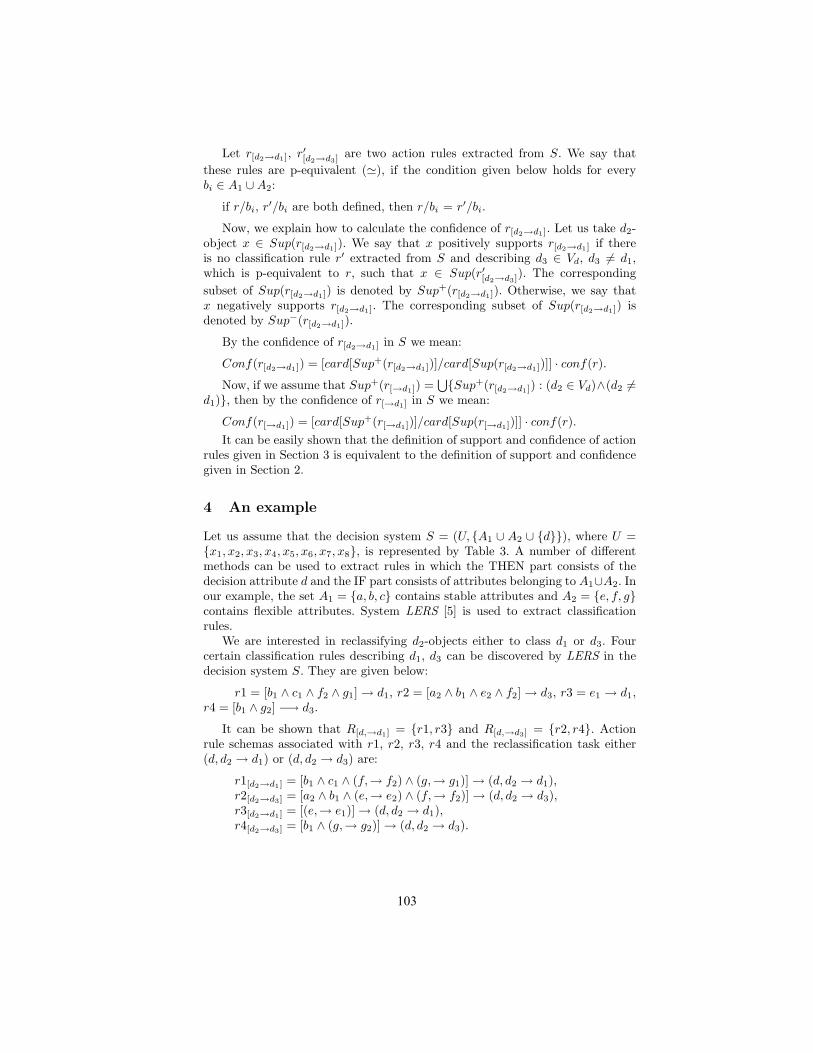
Let r[d2→d1], r′[d2→d3]are two action rules extracted from S. We say that

these rules are p-equivalent ('), if the condition given below holds for everybi ∈ A1 ∪A2:

if r/bi, r′/bi are both defined, then r/bi = r′/bi.

Now, we explain how to calculate the confidence of r[d2→d1]. Let us take d2-object x ∈ Sup(r[d2→d1]). We say that x positively supports r[d2→d1] if thereis no classification rule r′ extracted from S and describing d3 ∈ Vd, d3 6= d1,which is p-equivalent to r, such that x ∈ Sup(r′[d2→d3]

). The correspondingsubset of Sup(r[d2→d1]) is denoted by Sup+(r[d2→d1]). Otherwise, we say thatx negatively supports r[d2→d1]. The corresponding subset of Sup(r[d2→d1]) isdenoted by Sup−(r[d2→d1]).

By the confidence of r[d2→d1] in S we mean:

Conf(r[d2→d1]) = [card[Sup+(r[d2→d1])]/card[Sup(r[d2→d1])]] · conf(r).

Now, if we assume that Sup+(r[→d1]) =⋃{Sup+(r[d2→d1]) : (d2 ∈ Vd)∧(d2 6=

d1)}, then by the confidence of r[→d1] in S we mean:

Conf(r[→d1]) = [card[Sup+(r[→d1])]/card[Sup(r[→d1])]] · conf(r).It can be easily shown that the definition of support and confidence of action

rules given in Section 3 is equivalent to the definition of support and confidencegiven in Section 2.

4 An example

Let us assume that the decision system S = (U, {A1 ∪ A2 ∪ {d}}), where U ={x1, x2, x3, x4, x5, x6, x7, x8}, is represented by Table 3. A number of differentmethods can be used to extract rules in which the THEN part consists of thedecision attribute d and the IF part consists of attributes belonging to A1∪A2. Inour example, the set A1 = {a, b, c} contains stable attributes and A2 = {e, f, g}contains flexible attributes. System LERS [5] is used to extract classificationrules.

We are interested in reclassifying d2-objects either to class d1 or d3. Fourcertain classification rules describing d1, d3 can be discovered by LERS in thedecision system S. They are given below:

r1 = [b1 ∧ c1 ∧ f2 ∧ g1] → d1, r2 = [a2 ∧ b1 ∧ e2 ∧ f2] → d3, r3 = e1 → d1,r4 = [b1 ∧ g2] −→ d3.

It can be shown that R[d,→d1] = {r1, r3} and R[d,→d3] = {r2, r4}. Actionrule schemas associated with r1, r2, r3, r4 and the reclassification task either(d, d2 → d1) or (d, d2 → d3) are:

r1[d2→d1] = [b1 ∧ c1 ∧ (f,→ f2) ∧ (g,→ g1)] → (d, d2 → d1),r2[d2→d3] = [a2 ∧ b1 ∧ (e,→ e2) ∧ (f,→ f2)] → (d, d2 → d3),r3[d2→d1] = [(e,→ e1)] → (d, d2 → d1),r4[d2→d3] = [b1 ∧ (g,→ g2)] → (d, d2 → d3).

103

Table 3. Decision System

U a b c e f g d

x1 a1 b1 c1 e1 f2 g1 d1

x2 a2 b1 c2 e2 f2 g2 d3

x3 a3 b1 c1 e2 f2 g3 d2

x4 a1 b1 c2 e2 f2 g1 d2

x5 a1 b2 c1 e3 f2 g1 d2

x6 a2 b1 c1 e2 f3 g1 d2

x7 a2 b3 c2 e2 f2 g2 d2

x8 a2 b1 c1 e3 f2 g3 d2

We can also show that U[r1,d2] = Sup(r1[d2→d1]) = {x3, x6, x8}, U[r2,d2] =Sup(r2[d2→d3]) = {x6, x8}, U[r3,d2] = Sup(r3[d2→d1]) = {x3, x4, x5, x6, x7, x8},U[r4,d2] = Sup(r4[d2→d3]) = {x3, x4, x6, x8}.

Following AR(r1, d2) algorithm we get: [b1 ∧ c1 ∧ a1]? = {x1} 6⊆ U[r1,d2],[b1 ∧ c1 ∧ a2]? = {x6, x8} ⊆ U[r1,d2], [b1 ∧ c1 ∧ f3]? = {x6} ⊆ U[r1,d2], [b1 ∧c1 ∧ g2]? = {x2, x7} 6⊆ U[r1,d2], [b1 ∧ c1 ∧ g3]? = {x3, x8} ⊆ U[r1,d2]. It willgenerate two action rules: [b1 ∧ c1 ∧ (f, f3 → f2) ∧ (g,→ g1)] → (d, d2 → d1),[b1 ∧ c1 ∧ (f,→ f2) ∧ (g, g3 → g1)] → (d, d2 → d1).

In a similar way we construct action rules from the remaining three actionrule schemas.

The action rules discovery process, presented above, is called ARoGS andit consists of two main modules. For its further clarification, we use anotherexample which has no connection with Table 3. The first module extracts allclassification rules from S following LERS strategy. Assuming that d is the de-cision attribute and user is interested in re-classifying objects from its value d1

to d2, we treat the rules defining d1 as seeds and build clusters around them.For instance, if A1 = {a, b, g} are stable attributes, A2 = {c, e, h} are flexible inS = (U,A1∪A2∪{d}), and r = [[a1∧ b1∧ c1∧e1] → d1] is a classification rule inS, where Va = {a1, a2, a3}, Vb = {b1, b2, b3}, Vc = {c1, c2, c3}, Ve = {e1, e2, e3},Vg = {g1, g2, g3}, Vh = {h1, h2, h3}, then we remove from S all tuples containingvalues a2, a3, b2, b3, c1, e1 and we use again LERS to extract rules from this sub-system. Each rule defining d2 is used jointly with r to construct an action rule.The validation step of each of the set-inclusion relations, in the second module ofARoGS, is replaced by checking if the corresponding term was marked by LERSin the first module of ARoGS.

5 Conclusion

System ARoGS differs from the tree-based strategies for action rules discovery(for instance from DEAR [11]) because clusters generated by its second moduleare formed around target classification rules. An action rule can be constructed

104

in ARoGS from two classification rules only if both of them belong to the samecluster and one of them is a target classification rule. So, the complexity of thesecond module of ARoGS is 0(k ·n), where n is the number of classification rulesextracted by LERS and k is the number of clusters. The time complexity of thesecond module of DEAR is equal to 0(n · n), where n is the same as in ARoGS.The first module of ARoGS is the same as the first module of DEAR, so theircomplexities are the same.

6 Acknowledgements

This research was partially supported by the National Science Foundation undergrant IIS-0414815.

References

1. Adomavicius, G., Tuzhilin, A. (1997) Discovery of actionable patterns in databases:the action hierarchy approach, in Proceedings of KDD′97 Conference, New-port Beach, CA, AAAI Press

2. Dardzinska, A., Ras, Z.W., ”Extracting Rules from Incomplete Decision Systems:System ERID”, in Foundations and Novel Approaches in Data Mining, (Eds. T.Y.Lin, S. Ohsuga, C.J. Liau, X. Hu), Advances in Soft Computing, Vol. 9, Springer,2006, 143-154

3. Hilderman, R.J., Hamilton, H.J. (2001) Knowledge Discovery and Measuresof Interest, Kluwer

4. Greco, S., Matarazzo, B., Pappalardo, N., Slowinski, R. (2005) Measuring expectedeffects of interventions based on decision rules, in Journal of Experimental andTheoretical Artificial Intelligence, Taylor Francis, Vol. 17, No. 1-2

5. Grzymala-Busse, J. (1997) A new version of the rule induction system LERS, inFundamenta Informaticae, Vol. 31, No. 1, 27-39

6. Pawlak, Z., (1991) Information systems - theoretical foundations, in InformationSystems Journal, Vol. 6, 205-218

7. Silberschatz, A., Tuzhilin, A., (1995) On subjective measures of interestingness inknowledge discovery, in Proceedings of KDD′95 Conference, AAAI Press

8. Ras, Z., Wieczorkowska, A. (2000) Action Rules: how to increase profit of a com-pany, in Principles of Data Mining and Knowledge Discovery, LNAI, No.1910, Springer, 587-592

9. Ras, Z.W., Tzacheva, A., Tsay, L.-S. (2005) Action rules, in Encyclopedia ofData Warehousing and Mining, (Ed. J. Wang), Idea Group Inc., 1-5

10. Ras, Z.W., Dardzinska, A. (2006) Action rules discovery, a new simplified strategy,in Foundations of Intelligent Systems, F. Esposito et al. (Eds.), LNAI, No.4203, Springer, 445-453

11. Tsay, L.-S., Ras, Z.W. (2005) Action rules discovery system DEAR, method andexperiments, in Journal of Experimental and Theoretical Artificial Intel-ligence, Taylor & Francis, Vol. 17, No. 1-2, 119-128

12. Tsay, L.-S., Ras, Z.W. (2006) Action rules discovery system DEAR3, in Founda-tions of Intelligent Systems, LNAI, No. 4203, Springer, 483-492

13. Tzacheva, A., Ras, Z.W. (2005) Action rules mining, in International Journalof Intelligent Systems, Wiley, Vol. 20, No. 7, 719-736

105

Discovering Word Meanings Based on Frequent Termsets1

Henryk Rybinski*, Marzena Kryszkiewicz*, Grzegorz Protaziuk*, Aleksandra Kontkiewicz*, Katarzyna Marcinkowska, Alexandre Delteil**

*Warsaw University of Technology, **France Telecome R&D {hrb,mkr, gprotazi@ii.pw.edu.pl}, {akontkie, kmarcink}@elka.pw.edu.pl,

alexandre.delteil@orange-ft.com

Abstract. Word meaning ambiguity has always been an important problem in information retrieval and extraction, as well as, text mining (documents clustering and classification). Knowledge discovery tasks such as automatic ontology building and maintenance would also profit from simple and efficient methods for discovering word meanings. The paper presents a novel text mining approach to discovering word meanings. The offered measures of their context are expressed by means of frequent termsets. The presented methods have been implemented with efficient data mining techniques. The approach is domain- and language-independent, although it requires applying part of speech tagger. The paper includes sample results obtained with the presented methods.

Keywords: association rules, frequent termsets, homonyms, polysemy

1. Introduction

Discovery of word sense is what lexicographers do by profession. Automating this process has a much shorter history. First attempts were made in the 1960s by Sparck Jones [15]. In modern text mining and information retrieval, knowing the exact sense (or meaning) of a word in a document or a query becomes an important issue. It is considered that knowledge of an actual meaning of a polysemous word can considerably improve the quality of the information retrieval process by means of retrieving more relevant documents or extracting relevant information from the documents.

As sufficiently large corpora and efficient computers have become available, several attempts to automate the process have been undertaken. An overview of methods that have used artificial intelligence, machine readable dictionaries (knowledge-based methods) or corpora (knowledge-poor methods) can be found in [7], [12].

Many other text processing and knowledge management tasks, such as automatic translation, information extraction or ontology comparison, also require the ability to detect an actual meaning of a word.

1 The work has been performed within the project granted by France Telecom

106

The importance of polysemy detection becomes even clearer when one looks at the statistics for the English language. As stated in [10]:

“It has been estimated that more than 73% of words used in common English texts are polysemous, i.e., more than 73% of words have more than one sense.”

One should also note that many of those 73% words are highly polysemous. As stated in [9], an estimate of the average number of senses per word for all words found in common English texts is about 6.55. Therefore, there is a great need for methods able to distinguish polysemous words, as well as, their meanings.

Unfortunately, manually created dictionaries, which tend to ignore domain specific word senses, are not sufficient for the above mentioned applications. For this reason an amount of research concerning algorithms for automatic discovery of word senses from text corpora was carried out. An excellent survey of the history of ideas used in word sense disambiguation is provided by Ide and Veronis [7].

As for today, no satisfactory method has been described in the literature for discovering word meanings. However, a few methods that address this problem merit attention. Two main strategies for finding homonyms described in the literature are: Word Sense Discrimination (WSDc), i.e. the task of grouping the contexts that represent the senses of a polysemous word, and Word Sense Disambiguation (WSDa), i.e. the task of automatic labeling of polysemous words with a sense tag taken from a predefined set, [12]. There are a couple of different approaches to Word Sense Discrimination, as vector or cluster based, for example. The first one treats words as numeric vectors, whereas the second groups words with similar meaning into clusters. Most methods, however, use word distributional data and statistical analysis.

In the presented paper a novel text mining approach to discovery of homonyms is presented. The method applies the Word Sense Discrimination strategy, carrying out only shallow text analysis, which is restricted to the recognition of parts of speech, and is domain-independent. The method consists in determining atomic contexts of terms of interest by means of maximal frequent termsets, which then are used for determining discriminant contexts.

The rest of the paper is organized as follows: some relevant examples of WSDc systems are described in Section 2. Section 3 presents a deeper analysis of the problem as well as the basic ideas and concepts of the proposed method. The experiments and their results are presented in Section 4. Finally, Section 5 concludes the paper.

2. Related Work

As mentioned above, during the past years, a number of various approaches for the discovery of word senses and meanings have been proposed [7]. In [8] and [11] the authors describe a set of problems that are faced, when applying them to real data. The main ones are: data sparseness, infrequent meanings, overlapping meanings and the use of part-of-speech tags. Some of them are described in more detail below.

The method Clustering by Committee, introduced in [11], is based on grammatical relations between words. It requires that all documents are POS tagged and, what is

107

also important, grammatically correct. Each word in this method is represented as a feature vector, where each feature corresponds to a context that the word in question appears in. After computing all vectors, words considered as similar are grouped into clusters. Each cluster represents a single meaning. Finally, for each word the most similar clusters, with respect to a given minimal similarity measure value, are determined. These closest clusters constitute all discovered meanings of a word. The authors claim, that this method discovers also less frequent senses of a word and avoids discovering duplicate senses.

Another group of methods used for discovering word senses are Bayesian networks [16]. These methods are based on the statistical analysis and can be used in the situations, when only small or insufficient amount of data is available, e.g. when larger amount of data would prevent the system from being able to handle it. A Bayesian network is built using local dependencies between words. In such a network, each node represents a word, and an edge represents a conditional probability of the connected nodes. Bayesian networks can be used to determine a probability of co-occurrence of a set of words.

Markov clustering method [2] concentrates on analyzing texts written in a natural language. This method allows discovering the meanings of words used by examined group within a particular range. It follows an assumption, that nouns which frequently appear together in a list, are also semantically related. A result of the Markov clustering is a graph, where nouns co-occurring with appropriate frequency are connected with an edge. The ambiguous words are those that are connected with disjunctive parts of such a graph.

The main concern indicated in many papers is the size of the repositories, on which the experiments are carried out. Too little data leads to data sparseness problems; too much data causes the memory lack problems. In addition, current part-of-speech taggers still occasionally fail to produce the correct results, thus leading to errors.

In most cases, the methods for discovering meanings require the use of a predefined set of meanings for a word, which is their main disadvantage. Usually, the methods require checking of found meanings against those contained by a semantic dictionary, thesaurus, ontology etc., which are not easily available. It is therefore desired to develop other methodologies that could also give satisfactory results for the cases of a limited lexical support. Such methodologies are known as “knowledge-poor”.

The new method proposed in the paper satisfies this constraint, compromising both simplicity and sufficient efficiency. It also manages to handle the problem of overlapping meanings, as well as data sparseness and infrequent meanings.

3. Homonyms and Maximal Frequent Termset Contexts

Distinct meanings of homonyms are indicated by various distinct contexts in which they appear frequently. This assumption is based on the distributional hypothesis [5], where the underlying idea is that "a word is characterized by the company it keeps". The rule is very intuitive and therefore is applied to the proposed approaches. The problem is, however, how the notion of a context is defined. For example, it can be

108

understood as a set of words surrounding a target word frequently enough in documents, paragraphs, or sentences.

In our approach, a context is evaluated with respect to paragraphs as below. Let dictionary D = {t1, t2, ..., tm} be a set of distinct words, called terms. In general,

any set of terms is called a termset. The set P is a set of paragraphs, where each paragraph P is a set of terms such that P ⊆ P.

Statistical significance of a termset X is called support and is denoted by sup(X). sup(X) is defined as the number (or percentage) of paragraphs in P that contain X. Clearly, the supports of termsets that are supersets of termset X are not greater than sup(X).

A termset is called frequent if it occurs in more than ε paragraphs in P, where ε is a user-defined support threshold.

In the sequel, we will be interested in maximal frequent termsets, which we will denote by MF and define as the set of all maximal (in the sense of inclusion) termsets that are frequent.

Let x be a term. By MF(x) we denote all maximal frequent termsets containing x. MF(x) will be used for determining atomic contexts for x.

A termset X, x ∉ X, is defined as an atomic context of term x if {x}∪X is an element of MF(x). The set of all atomic contexts of x will be denoted by AC(x):

AC(x) = {X\{x}| X ∈ MF(x)}.

Clearly, for each two termsets Y, Z in AC(x), Y differs from Z by at least one term and vice versa. In spite of this, Y and Z may indicate the same meaning of x in reality. Let y be a term in Y\Z and z be a term in Z\Y and {xyz} be a termset the support of which is significantly less than the supports of Y and Z. This may suggest that Y and Z probably represent different meanings of x. Otherwise, Y and Z are likely to represent the same meaning of x. Please, note that {xyz} plays a role of a potential discriminant for pairs of atomic contexts. The set of all potential discriminants for Y and Z in AC(x) will be denoted by D(x, Y, Z):

D(x, Y, Z) = {{xyz}| y∈Y\Z ∧ z∈Z\Y}.

Among the potential discriminants, those which are relatively infrequent are called proper discriminants. Formally, the set of all proper discriminants for Y and Z in AC(x) will be denoted by PD(x, Y, Z), and defined as follows:

PD(x, Y, Z) = {X∈D(x, Y, Z)| relSup(x, X, Y, Z) ≤ δ}, where

relSup(x, X, Y, Z) = sup(X) / min(sup(xY), sup(xZ)), and

δ is a user-defined threshold.

In the sequel, relSup(x, X, Y, Z) is called a relative support of discriminant X for term x with respect to atomic contexts Y and Z.

Our proposal of determining the groups of contexts representing separate meanings of x is based on the introduced notion of proper discriminants for pairs of atomic contexts.

109

Atomic contexts Y and Z in AC(x) are called discriminable if there is at least one proper discriminant in PD(x, Y, Z). Otherwise, Y and Z are called indiscriminable.

A sense-discriminant context SDC(x, X) of x for termset X in AC(x) is defined as the family of those termsets in AC(x) that are indiscriminable with X; that is,

SDC(x, X) = {Y ∈ AC(x)| PD(x, X, Y) = ∅}.

Clearly, X ∈ SDC(x, X). Please, note that sense-discriminant contexts of x for Y and Z, where Y ≠ Z, may overlap, and in particular, may be equal.

The family of all distinct sense-discriminant contexts will be denoted by FSDC(x):

FSDC(x) = {SDC(x, X)| X ∈ AC(x)}.

Please, note that |FSDC(x)| ≤ |AC(x)|. A given term x is defined as a homonym candidate if the cardinality of FSDC(x)

is greater than 1. Final decision on homonymy is given to the user. Let us also note that the more overlapping are distinct sense-discriminant contexts, the more difficult is reusing the contexts for the meaning recognition in the mining procedures.

In order to illustrate the introduced concepts below we consider an example, which is based on an experimentally prepared set of documents. Example 1. A special repository has been built based on Google search engine and the AMI-SME software [3]. For the term apple, the following maximal frequent termsets have been found in the repository (see Table 1):

Table 1. Maximal frequent termsets for term apple (MF(apple))

Maximal frequent termset Support apple species breeding 1100 apple eat 14000 apple genetics 1980 apple gmo 1480 apple,botanics 2510 apple cake 3600 apple genome 1800 apple motherboard 2500 apple mouse pad 2500 apple iphone 6000

From this table we can evaluate the set of atomic contents, which is:

AC(apple) ={{species, breeding}, {eat}, {genetics}, {gmo}, {botanics}, {cake}, {genome}, {motherboard}, {mouse, pad}, {iphone}}.

Given the threshold δ = 0.2, we can evaluate the set of proper discriminants from the set of the potential discriminants {apple, z, y}. For instance, for the atomic contexts Y and Z such that Y = {species, breeding} and Z = {motherboard}, we have the following potential discriminants D(apple, Y, Z) = {{apple, species,

110

motherboard}, {apple, breeding, motherboard}}. Given the supports of the potential discriminants (see Table 2): sup({apple, species, motherboard}) = 209 and sup({apple, breeding, motherboard}) = 78, we can calculate their relative supports with respect to the supports of Y and Z as follows:

• relSup(apple, {apple, species, motherboard}, Y, Z) = sup({apple, species, motherboard}) / min(sup({apple, species, breeding}), sup(apple, motherboard)) = 209 / min(1100, 2500) = 0.19;

• relSup(apple, {apple, breeding, motherboard}, Y, Z) = sup({apple, breeding, motherboard}) / min(sup({apple, species, breeding}), sup(apple, motherboard)) = 78 / min(1100, 2500) = 0.07.

Both discriminants {apple, species, motherboard} and {apple, breeding, motherboard} have been found as proper, since their relative supports are below the threshold δ. The set of all proper discriminants is provided in Table 2.

Table 2. Proper discriminants

PD Support Relative support

Apple,species,motherboard 209 209/1100=0.19 Apple,breeding,motherboard 78 78/1100=0.07 Apple,eat motherboard 307 307/2500=0.12 Apple, botanics motherboard 68 68/2500=0.03 Apple,botanics,mouse 482 482/2500=0.19 Apple genome motherboard 74 74/1800=0.04 Apple genome pad 192 192/1800=0.10 Apple gmo motherboard 25 25/1800=0.10 Apple, breeding, iphone 0 0/1100=0.00 Apple, botanics, iphone 209 209/2500=0.08

For this set of proper discriminants we have found two sense-discriminant contexts

for the term apple: FSDC(apple) ={{apple, species, breeding, eat, genetics, gmo, botanics, cake}, {apple, motherboard, mouse, pad, iphone}}.

4. Homonyms discovering procedure

Text preprocessing phase The text preprocessing phase has been performed with the text mining platform TOM, which has been implemented at Warsaw University of Technology with the aim to support ontology maintenance and building with text mining techniques [13], [14]. The TOM platform provides options for defining the granularity of the text mining

111

process. In particular, TOM allows viewing the whole corpus as a set of documents, paragraphs or sentences. For the experiments of discovering homonyms, we set the granularity at the paragraph level. Thus, the first step was to generate a set of paragraphs from all the documents in the repository. It means that the context of particular terms is restricted to the paragraphs.

Then we have used the Hepple tagger [6] for part-of-speech tagging of the words in the sentences. In TOM, the tagger is a wrapped code of the Gate part of speech processing resource [4].

Conversion into “transactional database” The next step is to convert the text corpora into “transactional database” (in terms of [1]). So, every unit of text (i.e. every paragraph) is converted into a transaction containing a set of terms identifiers. The usage of terms identifiers instead of terms themselves leads to speeding up all the data mining operations. Further on, the identifiers of all terms that do not have required minimum support ε are deleted from all the transactions.

Finding maximal termsets Having reduced transaction representation of the text, we find the maximal frequent termsets MF(x) for all terms x from the list of terms of interest by means of any efficient data mining algorithm discovering maximal frequent itemsets [17].

Identification of the sense-discriminant contexts Having MF(x) for each term x, we calculate the atomic contexts AC(x) by simple removal of x from each termset in MF(x). For later use, for each atomic context X in AC(x), we store the support of the maximal frequent termset xX, from which X was derived. Now, we create potential discriminants for all the pairs of atomic contexts. Then, from the set of potential discriminants, we search for proper discriminants. This requires the calculation of the relative supports of the potential discriminants based on the supports of termsets xX, where X∈AC(x), and the supports of the potential discriminants themselves. While the supports of termsets xX, where X∈AC(x), are already known, the supports of the potential discriminants must be calculated. This is achieved with one scan over the transaction dataset [1]. Eventually, we calculate all the distinct sense-discriminant contexts for x. If the number of the distinct sense-discriminant contexts for the term x is higher than 1, we classify x as a polysemous term with the meanings determined by the contexts.

4. Experiments

Some experiments were conducted to measure the efficiency of the proposed algorithms. In general the found homonymous words can be classified into three different groups: a) Same meaning: berlin

[ ontology, european, intelligence, th, proceedings, workshop, eds, conference, learning, germany, artificial, august, ecai, hastings, wiemer- ] [ springer-, verlag ]

112

b) Different meaning: background [ domain, theory ] [ web, pages ]

c) Different use: results [ table, taxonomy, phase, similarity, measures ] [ information, users, queries ]

In our case, we are interested in discovering words which belong to the second and third group. The tests were done using different minimal support values and part-of-speech tags. So far better results were obtained with using smaller values for the support threshold. As the aim is to find homonymous nouns only those were considered. As for the contexts we took into account nouns, adjectives and verbs.

First, the tests have been performed on a repository composed of scientific papers dealing with ontologies, semantic web and text mining. The results have been rather modest, which can be justified by the fact that the scientific texts in a limited domain use homogeneous and well defined terminology. Nevertheless, for the term background two sense discriminant contexts have been found {domain, theory} and {web, pages}

Another group of tests have been performed on the Reuters repository. In this case the polysemous words are provided in Table 3.

Table 3 Results for the Reuters repository (the threshold set to 11 occurrences) President chinese jiang zemin

hussein iraqi saddam Ltd pictures seagram unit universal

corp murdoch news percent shares worth

York consolidated exchange stock trading city gate prices

France budget currency deficits brazil cup world

One can see an erroneous candidate president, which results from a shallow

semantic analysis of the text. With a deeper processing of the text (in this case replacing the proper names by tokens) the candidate would be rejected.

The term york has two meanings – one with the stock, and another one with the city. And with the third example, the term france has assigned the context referring to the country (economic situation) and the national football team.

The last group of tests referred to a repository composed from a set of queries in the AMI-SME system. These tests were oriented towards an experiment in checking the relevance of the idea and was used to find out meanings for the term apple (Example 1) and the term turkey. For both terms the method has proven its efficiency. Now, we plan performing more tests in order to determine the relevance and precision of the method.

113

5. Conclusions and Future Work

As said above, the tests were carried out on three repositories. As the results shown, the repository of scientific papers was not well suited for such experiments. The experiments with the Reuters repository have shown strong dependency on the size of the repository. With the too small repository, the results are rather poor. With the extended repository, we were able to find more polysemous words, on the other hand though, with too large repository we had problems with the data mining algorithms. To this end we have decided to define a priori a list of terms for which the experiment is run.

The results obtained so far show that the method presented above is able to distinguish homonymous words correctly. A human expert can easily interpret the contexts generated by the algorithms. Obviously there are among candidate erroneous terms, one can also expect that there are some undiscovered. This results from the following problems: (a) wrong part-of-speech tags assigned to the words by the POSTagger; (b) the values set for the minimal support, which are too high, but on the other hand, if lowered, caused memory problems; (c) the repository is too small and does not cover proper discriminants.

References

1. Agrawal R., Srikant R.: “Fast Algorithms for Mining Association Rules”. Proc. of the 20th Int’l Conf. on Very Large Databases, Santiago, 1994. Morgan Kaufmann 487–499

2. Dorow B. and Widdows D., “Discovering Corpus-Specific Word Senses”, EACL 2003, pp.79-82 Budapest, Hungary

3. Gawrysiak P., Rybinski H., Skonieczny Ł., Wiech P., "AMI-SME: An Exploratory Approach to Knowledge Retrieval for SME's," 3rd Int’l Conf. on Autonomic and Autonomous Systems (ICAS'07), 2007

4. General Architecture for Text Engineering. http://gate.ac.uk/projects.html 5. Harris, Z. (1954). Distributional structure. Word, 10(23): 146-162. 6. Hepple, M.: Independence and commitment: Assumptions for rapid training and execution

of rule-based POS taggers. In: Proc. of the 38th Annual Meeting of the Association for Computational Linguistics (ACL-2000) (2000)

7. Ide N, Veronis J., Introduction to the special issue on word sense disambiguation: The state of the art. Computational Linguistics 24(1):1–40. Special Issue on Word Sense Disambiguation.

8. Lin D., “Automatic Retrieval and Clustering of Similar Words”, in Proceedings of the 17th international conference on Computational linguistics - Volume 2, Canada, 1998

9. Mihalcea, R., and Moldovan, D., 2001, “Automatic Generation of a Coarse Grained WordNet,” in Proceedings of NAACL Workshop on WordNet and Other Lexical Resources, Pittsburgh, PA, June 2001.

10. Miller, G., Chadorow, M., Landes, S., Leacock, C., and Thomas, R. G., 1994, “Using a semantic concordance for sense identification.” Proc. of the ARPA Human Language Technology Workshop, pp. 240-243.

11. Pantel, P. and Lin, D. 2002. Discovering word senses from text. In Proceedings of the Eighth ACM SIGKDD international Conference on Knowledge Discovery and Data Mining (Edmonton, Alberta, Canada, July 23 - 26, 2002). KDD '02. ACM Press, New York, NY, 613-619.

114

12. Portnoy D., Unsupervised Discovery of the Multiple Senses of Words and Their Parts of Speech, The School of Engineering and Applied Science of The George Washington University, September 30, 2006

13. Protaziuk G., Kryszkiewicz M, Rybinski H, Delteil A., “Discovering Compound and Proper Nouns”, Rough Sets and Intelligent Systems Paradigms, Springer, LNAI 4595, pp. 505-515, 2007

14. Rybinski H., Kryszkiewicz M., Protaziuk G., Jakubowski A., Delteil A. Discovering Synonyms based on Frequent Termsets”, Rough Sets and Intelligent Systems Paradigms, Springer, LNAI 4595, pp. 516-525, 2007

15. Sparck Jones K., Synonymy and Semantic Classification, Edinburgh University Press, ISBN 0-85224-517-3, 1986 (originally published in 1964).

16. Young C. Park, Young S. Han and Key-Sun Choi “Automatic Thesaurus Construction using Bayesian Networks”, in the Proceedings of the fourth international conference on Information and knowledge management, United States, 1995

17. Zaki Mohammed J., Gouda Karam, Efficiently Mining Maximal Frequent Itemsets in 1st IEEE International Conference on Data Mining , San Jose, November 2001

115

Feature Selection: Near Set Approach

James F. Peters1, Sheela Ramanna2?

1Department of Electrical and Computer Engineering,University of Manitoba

Winnipeg, Manitoba R3T 5V6 Canadajfpeters@ee.umanitoba.ca

2 Department of Applied Computer Science,University of Winnipeg,

Winnipeg, Manitoba R3B 2E9 Canadas.ramanna@uwinnipeg.ca

Abstract. The problem considered in this paper is the description ofobjects that are, in some sense, qualitatively near each other and theselection of features useful in classifying near objects. The term qualita-tively near is used here to mean closeness of descriptions or distinctivecharacteristics of objects. The solution to this twofold problem is in-spired by the work of Zdzis law Pawlak during the early 1980s on theclassification of objects. In working toward a solution of the problem ofthe classification of perceptual objects, this article introduces a near setapproach to feature selection. Consideration of the nearness of objectshas recently led to the introduction of what are known as near sets, anoptimist’s view of the approximation of sets of objects that are more orless near each other. Near set theory started with the introduction ofcollections of partitions (families of neighbourhoods), which provide abasis for a feature selection method based on the information content ofthe partitions of a set of sample objects. A byproduct of the proposedapproach is a feature filtering method that eliminates features that areless useful in the classification of objects. This contribution of this articleis the introduction of a near set approach to feature selection.

Keywords: Description, entropy, feature selection, filter, informationcontent, nearness, near set, perception, probe function.

1 Introduction

The problem considered in this paper is the classification of perceptual objectsthat are qualitatively but not necessarily spatially near each other. The termqualitatively near is used here to mean closeness of descriptions or distinctivecharacteristics of objects. The solution to this problem is inspired by the work

? We gratefully acknowledge the very helpful comments, insights and corrections con-cerning this paper by Andrzej Skowron and the anonymous reviewers. This researchhas been supported by the Natural Sciences and Engineering Research Council ofCanada (NSERC) grants 185986 and 194376.

116

of Zdzis law Pawlak during the early 1980s on the classification of objects [12],elaborated in [13, 17], and a view of perception that is on the level of classesinstead of individual objects [10]. In working toward a solution of the problemof the classification of perceptual objects, this article introduces a nearness de-scription principle. An object description is defined by means of a vector of probefunction values associated with an object (see, e.g., [11]). Each probe function φi

represents a feature of an object of interest. Sample objects are near each otherif, and only if the objects have similar descriptions.

Ultimately, there is interest in selecting the probe functions [11] that leadto descriptions of objects that are minimally near each other. This is an essentialidea in the near set approach [7, 14, 16, 19] and differs markedly from the mini-mum description length (MDL) proposed in 1983 by Jorma Rissanen [23]. MDLdepends on the identification of possible data models and possible probabilitymodels. By contrast, NDP deals with a set X that is the domain of a descrip-tion used to identify similar objects. The term similar is used here to denote thepresence of objects that have descriptions that match each other to some degree.

The near set approach leads to partitions of ensembles of sample objectswith measurable information content and an approach to feature selection. Theproposed feature selection method considers combinations of n probe functionstaken r at a time in searching for those combinations of probe functions thatlead to partitions of a set of objects that has the highest information content.It is Shannon’s measure of the information content [8, 26] of an outcome thatprovides a basis for the proposed feature selection method. In this work, featureselection results from a filtering method that eliminates those features that havelittle chance to be useful in the analysis of sample data. The proposed approachdoes not depend on the joint probability of finding a feature value for an inputvectors that belong to the same class as in [6]. In addition, the proposed approachto measuring the information content of families of neighbourhoods differs fromthe rough set-based form of entropy in [25]. Unlike the dominance-relation roughset approach [5], the near set approach does not depend on preferential orderingof value sets of functions representing object features. The contribution of thisarticle is the introduction of a near set approach to feature selection.

This article has the following organization. A brief introduction to the nota-tion and basic approach to object description is given in Sect. 2. A brief introduc-tion to nearness approximation spaces is given in Sect. 4. A nearness descriptionprinciple is introduced in Sect. 3. A near set-based feature selection method isintroduced in Sect. 5.

2 Object Description

Objects are known by their descriptions. An object description is defined bymeans of a tuple of function values φ(x) associated with an object x ∈ X (see(1)). The important thing to notice is the choice of functions φi ∈ B used todescribe an object of interest.

Object Description : φ(x) = (φ1(x), φ2(x), . . . , φi(x), . . . , φL(x)). (1)

117

Table 1. Description Symbols

Symbol Interpretation

< Set of real numbers,O Set of perceptual objects,X X ⊆ O, set of sample objects,x x ∈ O, sample object,F A set of functions representing object features,B B ⊆ F ,φ φ : O → <L, object description,L L is a description length,i i ≤ L,φi φi ∈ B, where φi : O −→ <, probe function,

φ(x) φ(x) = (φ1(x), φ2(x), φ3(x), . . . , φi(x), . . . , φL(x)).

The intuition underlying a description φ(x) is a recording of measurementsfrom sensors, where each sensor is modelled by a function φi. Assume that B ⊆ F(see Table 1) is a given set of functions representing features of sample objectsX ⊆ O. Let φi ∈ B, where φi : O −→ <. The value of φi(x) is a measure-ment associated with a feature of an object x ∈ X. The function φi is called aprobe [11]. In combination, the functions representing object features provide abasis for an object description φ : O → <L, a vector containing measurements(returned values) associated with each functional value φi (x) in (1), where thedescription length |φ| = L.

2.1 Sample Behaviour Description

Table 2. Sample ethogram

xi s a p(s, a) r d

x0 0 1 0.1 0.75 1x1 0 2 0.1 0.75 0x2 1 2 0.05 0.1 0x3 1 3 0.056 0.1 1x4 0 1 0.03 0.75 1x5 0 2 0.02 0.75 0x6 1 2 0.01 0.9 1x7 1 3 0.025 0.9 0

By way of illustration, consider the description of the behaviour observablein biological organisms. For example, a behaviour can be represented by a tuple

(s, a, p(s, a), r)

where s, a, p(s, a), r denote organism functions representing state, action, actionpreference in a state, and reward for an action, respectively. A reward r is ob-

118

served in state s and results from an action a performed in the previous state.The preferred action a in state s is calculated using

p(s, a)← p(s, a) + βδ(s, a),

where β is the actor’s learning rate and δ(r, s) is used to evaluate the quality ofaction a (see [20]). In combination, tuples of behaviour function values form thefollowing description of an object x relative to its observed behaviour:

Organism Behaviour : φ(x) = (s(x), a(x), r(x), V (s(x))).

Table 2 exhibits a sample observed behaviours of an organism.

3 Nearness of Objects

Approximate, a [L. approximat-us to draw near to.]

A. adj.

1. Very near, in position or in character;

closely situated; nearly resembling.

–Oxford English Dictionary, 1933.

Table 3. Set, Relation, Probe Function Symbols

Symbol Interpretation

∼B {(x, x′) | f(x) = f(x′) ∀f ∈ B}, indiscernibility relation,[x]B [x]B = {x′ ∈ X | x′ ∼B x}, elementary granule (class),O/ ∼B O/ ∼B=

˘[x]B | x ∈ O

¯, quotient set,

ξB Partition ξB = O/ ∼B ,∆φi ∆φi = φi(x

′)− φi(x), probe function difference,

Sample objects X ⊆ O are near each other if, and only if the objects havesimilar descriptions. Recall that each description φ1 defines a description of anobject (see Table 1). Then let ∆φi denote

∆φi = φi(x′)− φi(x),

where x, x′ ∈ O (see Table 3). The difference ∆φ leads to a definition of theindiscernibility relation ∼B introduced by Zdzis law Pawlak [12] (see Def 1).1 In a more general setting that includes data mining, φi would be defined to allow

for non-numerical values, i.e., let φi : X −→ V , where V is the value set for therange of φi [22]. The more general definition of φi ∈ F is also better in setting forththe algebra and logic of near sets after the manner of the algebra and logic of roughsets [1, 3, 4, 22]. Real-valued probe functions are used in object descriptions in thisarticle because we have science and engineering applications of near sets in mind.

119

Definition 1 Indiscernibilty RelationLet x, x′ ∈ O, B ⊆ F .

∼B= {(x, x′) ∈ O ×O | ∀φi ∈ B � ∆φi = 0} ,where i ≤ description length |φ| .

Definition 2 Nearness Description Principle (NDP)Let B ⊆ F be a set of functions representing features of objects x, x′ ∈ O.Objects x, x′ are minimally near each other if, and only if there exists φi ∈B such that x ∼{φi} x′, i.e., ∆φi = 0.

In effect, objects x, x′ are considered minimally near each other wheneverthere is at least one probe function φi ∈ B so that φi(x) = φi(x′). A probefunction can be thought of as a model for a sensor (see, e.g., [11, 17]). Then φi

constitutes a minimum description of the objects x, x′ that makes it possible forus to assert that x, x′ are near each other. Ultimately, there is interest in iden-tifying the probe functions that lead to partitions with the highest informationcontent. The nearness description principle (NDP) differs markedly from min-imum description length (MDL) proposed by Jorma Rissanen [23]. MDL dealswith a set X = {xi | i = 1, . . . } of possible data models and a set Θ of possibleprobability models. By contrast, NDP deals with a set X that is the domainof a description φ : X −→ <L and the discovery of at least one probe functionφi(x) in a particular description φ(x) used to identify similar objects in X. Theterm similar is used here to denote the presence of objects x, x′ ∈ X and at leastone φi in object description φ, where x ∼φi

x′. In that case, objects x, x′ aresaid to be similar. This leads to a feature selection method, where one considerscombinations of n probe functions r in searching for those combinations of probefunctions that lead to partitions with the highest information content.

Observation 1 Near Objects in a ClassLet ξB = O/ ∼B denote a partition of O. Let [x]B ∈ ξB denote an equivalenceclass. Assume x, x′ ∈ [x]B. From Table 3 and Def. 1, we know that for eachφi ∈ B,∆φi = 0. Hence, from Def. 2, x, x′ are near objects.

Theorem 1 The objects in a class [x]B ∈ ξB are near objects.

Proof. The nearness of objects in a class in ξB follows from Obs. 1. �

4 Nearness Approximation Spaces

The original generalized approximation space (GAS) model [27] has recentlybeen extended as a result of recent work on nearness of objects (see, e.g., [7, 14,16, 18, 19, 28, 29]). A nearness approximation space (NAS) is a tuple

NAS = (O,F ,∼Br, Nr, νNr

),

defined using set of perceived objects O, set of probe functions F representingobject features, indiscernibility relation ∼Br defined relative to Br ⊆ B ⊆ F ,

120

Table 4. Nearness Approximation Space Symbols

Symbol Interpretation

B B ⊆ F ,Br r ≤ |B| probe functions in B,∼Br Indiscernibility relation defined using Br,[x]Br

[x]Br= {x′ ∈ O | x ∼Br x′}, equivalence class,

O/ ∼Br O/ ∼Br =n

[x]Br| x ∈ O

o, quotient set,

ξBr Partition ξO,Br = O/ ∼Br ,φi Probe function φi ∈ F ,r

`|B|r

´, i.e., |B| functions φi ∈ F taken r at a time,

Nr(B) Nr(B) = {ξBr | Br ⊆ B}, set of partitions,νNr νNr : P(O)× P(O) −→ [0, 1], overlap function,

Nr(B)∗X Nr(B)∗X =S

x:[x]Br⊆X [x]Br , lower approximation,

Nr(B)∗X Nr(B)∗X =S

x:[x]Br∩X [x]Br 6= ∅, upper approximation,

BndNr(B)(X) Nr(B)∗X\Nr(B)∗X = {x ∈ Nr(B)∗X | x /∈ Nr(B)∗X}.

family of neighbourhoods Nr, and neighbourhood overlap function νNr . Therelation ∼Br is the usual indiscernibility relation from rough set theory restrictedto a subset Br ⊆ B. The subscript r denotes the cardinality of the restrictedsubset Br, where we consider

(|B|r

), i.e., |B| functions φi ∈ F taken r at a time

to define the relation ∼Br. This relation defines a partition of O into non-empty,

pairwise disjoint subsets that are equivalence classes denoted by [x]Br, where

[x]Br= {x′ ∈ O | x ∼Br x′} .

These classes form a new set called the quotient set O/ ∼Br , where

O/ ∼Br=

{[x]Br

| x ∈ O}

.

In effect, each choice of probe functions Br defines a partition ξBron a set of

objects O, namely,ξBr = O/ ∼Br .

Every choice of the set Br leads to a new partition of O. The overlap functionνNr

is defined byνNr : P(O)× P(O) −→ [0, 1],

where P(O) is the powerset of O. The overlap function νNrmaps a pair of sets to

a number in [0, 1] representing the degree of overlap between sets of objects withfeatures defined by probe functions Br ⊆ B. For each subset Br ⊆ B of probefunctions, define the binary relation ∼Br

= {(x, x′) ∈ O ×O : ∀φi ∈ Br, φi(x) =φi(x′)}. Since each ∼Br

is, in fact, the usual indiscernibility relation [12], let[x]Br

denote the equivalence class containing x, i.e.,

[x]Br = {x′ ∈ O | ∀f ∈ Br, f(x′) = f(x)}.

121

If (x, x′) ∈ ∼Br(also written x ∼Br

x′), then x and x′ are said to be B-indiscernible with respect to all feature probe functions in Br. Then define acollection of partitions Nr(B) (families of neighbourhoods), where

Nr(B) = {ξBr | Br ⊆ B} .

Families of neighborhoods are constructed for each combination of probe func-tions in B using

(|B|r

), i.e., |B| probe functions taken r at a time. The family

of neighbourhoods Nr(B) contains a set of percepts. A percept is a byproductof perception, i.e., something that has been observed [9]. For example, a classin Nr(B) represents what has been perceived about objects belonging to a neigh-bourhood, i.e., observed objects with matching probe function values.

Definition 3 Near Sets Let X, X ′ ⊆ O, B ⊆ F . Set X is near X ′ if, and onlyif there exists x ∈ X, x′ ∈ X ′, φi ∈ B such that x ∼{φi} x′.

If X is near X ′, then X is a near set relative to X ′ and X ′ is a near set relativeto X. Notice that if we replace X ′ by X in Def. 3, then a set X containing nearobjects is a near set.

Theorem 2 Families of Neighbourhoods Theorem A collection of parti-tions (families of neighbourhoods) Nr(B) is a near set.

4.1 Sample Families of Neighbourhoods

Let X ⊆ O, B ⊆ F denote a set of sample objects {x0, x1, . . . , x7} and set offunctions {s, a, p, r}, respectively. Sample values of the state function s : X −→{0, 1} and action function a : X −→ {1, 2, 3} are shown in Table 2. Assumereward function r : A −→ [0, 1] and a preference function p : S × A −→ [0, 1].From Table 2, we can, for example, extract the collection of partitions N1(B)for r = 1.

X = {x0, x1, . . . , x7} ,

N1(B) ={ξ{s}, ξ{a}, ξ{p}, ξ{r}

}, where

ξ{s} = [x0]{s} , [x2]{s} ,

ξ{a} = [x0]{a} , [x1]{a} , [x3]{a} ,

ξ{p} = [x0]{p} , [x2]{p} , [x5]{p} , [x6]{p} ,

ξ{r} = [x0]{r} , [x2]{r} .

4.2 Information Content of a Partition

The Shannon information content of an outcome x is defined by

h (x) = log21

Pr (x),

122

which is measured in bits, where bit denotes a variable with value 0 or 1, andh(v) provides a measure of the information content of the event x = v [8], whichdiffers from the rough set-based form of entropy in [25]. The assumption madehere is that the event x = xi recorded in Table 2 is random and that a sample Xis symmetric, i.e., each event in the sample has the same probability. In effect,Pr(x = xi) = 1

|X| . The occurrence of a class [x]Br= [xi]Br

∈ ξBris treated

as a random event, and all classes in a partition ξBrare assumed to be equally

likely. Then, for example, there are 2 classes in the partition ξ{s} ∈ N1(B) andPr([x0] ∈ ξ{s}) = log2

112

= log22 = 1. The information content H(X) of anensemble X is defined to be the average Shannon information content of theevents represented by X.

H(X) =∑x∈X

Pr(x) · log21

Pr(x).

Then, for example, the information content of sample partitions in N1(B) ={ξ{s}, ξ{a}, ξ{p}, ξ{r}

}have the following information content.

H(ξ{s}) = H(ξ{r}) =12· log2

112

+12· log2

112

=12· 1 +

12· 1 = 1,

H(ξ{a}) =13· (3 · 1.59) = 1.59,

H(ξ{p}) =14· (4 · 2) = 2.

This suggests an approach to feature selection based on information content,which is computationally rather simple.

Algorithm 1: Partition SelectionInput : NAS = (O,F ,∼Br , Nr, νNr ), B ∈ F , choice r.Output: Partition size list Φ, where Φ [i] = number of classes in partition

ξBr ∈ Nr(B).Initialize i = 0;while (i ≤ |Nr(B)|) do

Select ith partition ξBr ∈ Nr(B);Φ [i] = |ξBr ∈ Nr(B)|;i = i + 1;

end

5 Feature Selection

A practical outcome of the near set approach is a feature selection method.Recall that each partition ξBr ∈ Nr(B) contains classes defined by the relation

123

Algorithm 2: Feature SelectionInput : Array Φ, where Φ [i] = number of classes in |ξBr ∈ Nr(B)|, threshold

th.Output: Ordered list Γ , where Γ [i] is a winning probe function.Initialize i = 0;Sort Φ in descending order based on the information content of ξBr ∈ Nr(B);while (i ≥ th) do

Γ [i] = Φ [i];i = i + 1;

end

∼Br . We are interested in the classes in each ξBr ∈ Nr(B) with informationcontent greater than or equal to some threshold th. The basic idea here is toidentify probe functions that lead to partitions with the highest informationcontent, which occurs in partitions with high numbers of classes. In effect, as thenumber of classes in a partition increases, there is a corresponding increase inthe information content of the partition. A list Φ of partition sizes is constructedusing Alg. 1. By sorting Φ based on information content using Alg. 2, we havea means of means of selecting tuples containing probe functions that definepartitions having the highest information content.

5.1 Sample Feature SelectionsN2(B) =

{ξ{s,a}, ξ{s,p}, ξ{a,p}, ξ{s,r}, ξ{a,r}, ξ{p,r}

}, where

ξ{s,a} ={

[x0]{s,a} , [x1]{s,a} , [x2]{s,a} , [x3]{s,a}

},

ξ{s,p} ={

[x0]{s,p} , [x2]{s,p} , [x3]{s,p} , [x4]{s,p} , [x5]{s,p} , [x6]{s,p} , [x7]{s,p}

},

ξ{a,p} ={

[x0]{a,p} , [x1]{a,p} , [x2]{a,p} , [x3]{a,p} , [x4]{a,p} , [x5]{a,p} , [x6]{a,p} , [x7]{a,p}

},

ξ{s,r} ={

[x0]{s,r} , [x2]{s,r} , [x6]{s,r}

},

ξ{a,r} ={

[x0]{a,r} , [x1]{a,r} , [x2]{a,r} , [x3]{a,r} , [x7]{a,r}

},

ξ{p,r} ={

[x0]{p,r} , [x2]{p,r} , [x3]{p,r} , [x4]{p,r} , [x5]{p,r} , [x6]{p,r}

}.

This section continues the exploration of the partitions in families of neighbour-hoods for each choice of r ≤ |B|. The observations in Table 2 were produced byan ecosystem simulation reported in [21]. The function values in Table 2 werediscretized using ROSE [24]. ROSE was used in this study because it allowsthe user to use as input a discretized table. This was important for us becauseTable 2 was discretized using a local Object Recognition System (ORS) toolset.The ORS discretized table was used to define the partition of the sample ob-jects in Table 2. Collections of partitions N2(B), N3(B) can be extracted fromTable 2 (in this section, N2(B) is given and the display of N3(B) is omitted tosave space).

124

5.2 Feature Selection Results

Table 5. Partition Information Content Summary

Fn H Fns H Fns H

ξ{s} 1.0 ξ{s,a} 2.0 ξ{s,a,p} 3.0ξ{a} 1.59 ξ{s,p} 2.8 ξ{a,p,r} 3.0ξ{p} 2.0 ξ{a,p} 3.0 ξ{s,a,r} 1.63ξ{r} 1.0 ξ{s,r} 1.58 ξ{s,p,r} 2.8

ξ{a,r} 1.46ξ{p,r} 1.63

In the single feature case (r = 1), functions a and p define partitions withthe highest information content for sample X represented by Table 2. Noticethat preference p is more important than a in the ecosystem experiments, be-cause p indicates the preferred action in a give state. In the two feature case (r= 2), feature combination a, p define a partition with the highest informationcontent, namely, 3 (see Table 5). If we set the threshold r ≥ 3, then featuresa, p (action, preference) are selected because the information content of partitionH(ξ{a,p}) = 3 in N2(B), which is also one of the reducts found by ROSE [24] us-ing Table 2 as input. Notice that a, p defines all of the high scoring partitions inTable 5. Similarly, for N3(B), the features s, a, p are selected, where the informa-tion content of H(ξ{s,a,p}) = 3 (highest) and H(ξ{s,a,r}) = 1.58 (lowest) whichis at variance with the findings by ROSE, which selects {s, a, r} as a reduct.Finally, notice that ROSE selects a as the core feature and the highest scoringpartitions defined by combinations of functions containing a.

5.3 Complexity Issue

Notice that the proposed feature selection method is based on collections ofpartitions, each contain a family of neighborhoods, constructed for each com-bination of probe functions in B using

(|B|r

), i.e., |B| probe functions taken r

at a time. Hence, the proposed method has very high complexity for large B.To achieve feature selection with polynomial time complexity, features are se-lected by considering only the partitions in N1(B). This approach can be usedto identify all of those partitions with information content H(ξf ) for partitionX/ ∼{f} defined relative to a single function f representing a feature of thesample objects. For recognition of sample objects with thousands of features,this approach is useful in an unsupervised learning environment2. More workneeds to be done on the proposed feature selection method to make it useful2 See, e.g. lymphocyte samples with genes representing 4026 features [2]. Assuming

that a maximum of m operations are required in each partition, then 4026 ·m oper-ations are necessary for feature selection for single feature partitions. By choosing a

125

in discovering reducts suitable for supervised learning for sample objects withmany features.

6 Conclusion

The proposed approach to the nearness of objects and sets and feature selectionbased on object description is a direct result of the original approach to theclassification of objects introduced by Zdzis law Pawlak during the early 1980s.Feature selection is based on measurement of the information content of the par-titions in each family of neighbourhoods. Future work will include considerationof the relation between the proposed feature selection method for large numbersof features for objects in various sample spaces.

References

1. Banerjee, M, Chakraborty, M.K.: Algebras from rough sets. In: Pal, S.K.,Polkowski, L., Skowron, A. (Eds.): Rough-neuro Computing: Techniques for Com-puting with Words. Springer, Berlin (2004) 157-184.

2. Banerjee, M., Mitra, S., Banka, H.: Evolutionary rough feature selection in geneexpression data, IEEE Transactions on Systems, Man, and Cybernetics–Part C:Applications and Reviews, 37(4) July (2007) 1-12.

3. Cattaneo, G., Ciucci, D.: Algebraic structures for rough sets, Transactions onRough Sets, vol. II, LNCS 3135 (2004) 63-101.

4. Duntsch, I.: A logic for rough sets, Theoretical Computer Science 179 (1997) 427-436.

5. Greco, S., Matarazzo, B., Slowinski, R.: Dominance-based rough set approachto knowledge discovery. In: N. Zhong, J. Liu (Eds.): Intelligent Technologies forInformation Analysis, Springer, Berlin (2004) 513-552.

6. Guyon, I., Gunn, S., Nikravesh, M., Zadeh, L.A. (Eds.): Feature Extraction. Foun-dations and Applications. Springer, Berlin (2006).

7. Henry, C., Peters, J.F.: Image Pattern Recognition Using Approximation Spacesand Near Sets, In: Proceedings of Eleventh International Conference on RoughSets, Fuzzy Sets, Data Mining and Granular Computing (RSFDGrC 2007), JointRough Set Symposium (JRS 2007), Lecture Notes in Artificial Intelligence, vol.4482 (2007) 475-482.

8. MacKay, D.J.C.: Information Theory, Inference, and Learning Algorithms, Cam-bridge University Press, UK (2003).

9. Murray, J.A., Bradley, H., Craigie, W., Onions, C.: The Oxford English Dictionary,Oxford University Press, London (1933).

10. Or lowska, E.: Semantics of Vague Concepts, Applications of Rough Sets, Institutefor Computer Science, Polish Academy of Sciences, Report 469 (1982).

11. Pavel, M.: Fundamentals of Pattern Recognition, 2nd Ed., Marcel Dekker, Inc.,NY (1993).

12. Pawlak, Z.: Classification of Objects by Means of Attributes, Institute for Com-puter Science, Polish Academy of Sciences, Report 429 (1981).

threshold th, it is then possible to select the most discriminating features useful inclassifying the lymphocyte samples.

126

13. Pawlak, Z., Skowron, A.: Rudiments of rough sets, Information Sciences, vol. 177(2007) 3-27.

14. Peters, J.F.: Near sets. Special theory about nearness of objects, Fundamenta In-formaticae, vol. 76, (2007) 1-28.

15. Peters, J.F.: Near sets. General theory about nearness of objects, Applied Math-ematical Sciences Journal (2007), in press.

16. Peters, J.F.: Near Sets. Toward Approximation Space-Based Object Recognition,In: Yao, Y., Lingras, P., Wu, W.-Z, Szczuka, M., Cercone, N., Slezak, D.,Eds., Proc. of the Second Int. Conf. on Rough Sets and Knowledge Technol-ogy (RSKT07), Joint Rough Set Symposium (JRS07), Lecture Notes in ArtificialIntelligence 4481, Springer, Berlin, (2007) 22-33.

17. Peters, J.F.: Classification of objects by means of features, In: Proc. IEEE Sym-posium Series on Foundations of Computational Intelligence (IEEE SCCI 2007),Honolulu, Hawaii (2007) 1-8.

18. Peters, J.F., Skowron, A., Stepaniuk, J.: Nearness in approximation spaces, G.Lindemann, H. Schlilngloff et al. (Eds.), Proc. Concurrency, Specification & Pro-gramming (CS&P’2006). Informatik-Berichte Nr. 206, Humboldt-Universitat zuBerlin (2006) 434-445.

19. Peters, J.F., Skowron, A., Stepaniuk, J.: Nearness of Objects: Extension of Ap-proximation Space Model, Fundamenta Informaticae, vol. 79 (2007) 1-24.

20. Peters J.F., Henry C., Gunderson D.S.:a Biologically-inspired approximate adap-tive learning control strategies: A rough set approach, International Journal ofHybrid Intelligent Systems, (2007) to appear.

21. Peters J.F., Henry C., Ramanna, S.: Rough Ethograms: Study of Intelligent Sys-tem behaviour. In: M.A. K lopotek, S. Wierzchon, K. Trojanowski (Eds.), NewTrends in Intelligent Information Processing and Web Mining (IIS05), Gdansk,Poland (2005) 117-126.

22. Polkowski, L.: Rough Sets. Mathematical Foundations. Springer-Verlag, Heidel-berg (2002).

23. J.J. Rissanen, A universal prior for integers and estimation by Minimum Descrip-tion Length. Annals of Statistics 11(2) (1983) 416-431.

24. Rough Sets Data Explorer, Version 2.2, c©1999-2002 IDSS,http://idss.cs.put.poznan.pl/site/software.html

25. Shankar, B.U.: Novel classification and segmentation techniques with applicationto remotely sensed images, Transactions on Rough Sets, vol. VII, LNCS 4400(2007) 295-380.

26. Shannon, C.E.: A mathematical theory of communication, Bell Systems TechnicalJournal 27 (1948) 279-423, 623-656.

27. Skowron, A., Stepaniuk, J.: Generalized approximation spaces. In: Lin,T.Y.,Wildberger, A.M. (Eds.), Soft Computing, Simulation Councils, San Diego(1995) 18-21.

28. Skowron, A., Swiniarski, R., Synak, P.: Approximation spaces and informationgranulation, Transactions on Rough Sets, vol. III (2005) 175-189.

29. Skowron, A., Stepaniuk, J., Peters, J.F., Swiniarski,R.: Calculi of approximationspaces, Fundamenta Informaticae, 72(1-3) (2006) 363–378.

127

Contextual Adaptive Clusteringwith Personalization

Krzysztof Ciesielski, Mieczys law A. K lopotek, S lawomir Wierzchon

Institute of Computer Science, Polish Academy of Sciences,ul. Ordona 21, 01-237 Warszawa, Polandkciesiel,klopotek,stw@ipipan.waw.pl

Abstract. We present a new method of modeling of cluster structureof a document collection and outline an approach to integrate additionalknowledge we have about the document collection like prior categoriza-tion of some documents or user defined / deduced preferences in theprocess of personalized document map creation.

1 Introduction

Clustering of Web documents, especially in large and heterogeneous collections,is a challenging task, both in terms of processing time complexity and clusteringquality.

But the most challenging part is the way how the clustering information isconveyed to the end user and how it meets his expectations (personalization).

Note that a text document is usually a very complex information structurefrom the point of view of human beings dealing with this document. But actuallya computer system fully understanding the document contents is beyond tech-nological possibilities. Therefore some kinds of approximation to the content aredone. Documents are frequently treated as a bag of words in computer models,and the documents are viewed as points in term-document vector space, but thisapproach turns out to be insufficient, hence more complex representations, bothof the content of a single document and their collections are investigated.

In the recent years, various projects (WebSOM, [11–13, 7], Themescape etc.)were aimed at developing a new form of cluster description a visual documentmap representation. In a two-dimensional space, consisting of quadratic or hexag-onal cells, the split into clusters is represented as an assignment of documentsto cells in such a way, that documents assigned to cells are as homogenous aspossible and cells (clusters) containing similar documents are placed close to oneanother on the map, and map regions are labeled with best-fitting terms fromthe documents. An inversion of the clustering (that is clustering of terms insteadof documents) is also possible.

It is generally believed that individual information needs of users may differand there is a general feeling that therefore also the data processing resultsshould accommodate to the profile of the user. Countless methods and ways ofuser profile representation and acquisition have been designed so far.

128

The problem with map-like representation of document collections, however,lies in the pretty expensive processing / high complexity (in terms of time andspace) so that a personalized ad-hoc representation is virtually impossible.

In the current paper we contest this view and claim that personalization ofmap representation of large scale document collections is possible by a care-ful separation of the concept of individual needs from the concept of commonknowledge. This leads to the possibility of separation of computationally intensetasks of identification of the structure of clustering space from the relatively lessresource consuming pure presentation part.

The paper is concerned with outlining the general concept, while the Readermay refer to our earlier papers for experimental results supporting validity ofpartial clams from which the current exposition is derived.

The paper is organized as follows: In section 2 the concept of cluster spaceis presented. Section 3 describes practical ways of cluster space approximationfrom data. Section 4 outlines possible ways of personalizing the maps presenta-tion. Last section, 5, summarizes the paper and gives some future directions forresearch.

2 Clustering Space

It is usually assumed that personalization is needed because of cultural, ethnicaletc. differences that influence the world of values, the attitudes and the views.So, in the particular case of clustering, the distances (or more strictly speakingdissimilarities) between the objects may change from person to person. So apersonalization under this assumption would be reduced to a total re-clusteringof the objects.

We disagree with this assumption. While avoiding here a deeper philosoph-ical discussion of the issue, let us point at some issues significant for the textprocessing task. Human beings possess to a large extent an objective world whichthey describe with a common set of concepts (a vocabulary) that is intended forthem to communicate to other human beings. So the vast majority of concepts isshared and their meaning not determined by values, attitudes etc. What differsthe human beings is the current task they are interested in. So if discussing e.g.an issue in biology, one does not care about concepts important for chemical en-gineering. Hence it is not the personal attitude, but rather the context in whichan issue is discussed that impacts the feeling of dissimilarity of opinions (in thiscase documents).

Therefore, in our opinion, the proper approach to personalization has to bewell founded on the proper representation of document information.

It has been generally agreed that the processing of textual information, es-pecially at large scale, requires a simplification of the document representation.So a document is treated as a bag of words (without bothering about sentencestructure). It is represented in the space of documents (with dimensions beingspread by words and phrases, that is terms) as a point with coordinates being

129

a function of the frequency of each term in the document. The similarity be-tween two documents is measured as a cosine of the angle between the vectorsdrawn from the original of the coordinate system to these points. Furthermore,dimensionality reduction may be of high importance [6]

So the weight of a term in the document is calculated as the so-called tfidf(term frequency times the inverse document frequency) computed according tothe formula:

wt,d = ft,d × log|D|f

(t)D

(1)

where ft,d is the number of occurrences of term t in document d, |D| is thecardinality of the set of documents, and f

(t)D is the number of documents in

collection D containing at least one occurrence of term t.A document d is described by a vector d = (wt1 , . . . , wt|T |), where T is

the set of terms. Usually, the document is turned into a normalized form d =(wt1 , . . . , wt|T |) where d has a unit length.

We notice immediately that the weights of terms in a document are influencedby their distribution in entire document collection. If we look, however, at anyprocess of clustering, we immediately notice that weights calculated by the verysame method, but within any reasonable (homogenous) cluster, not being arandom subsample of the whole collection, would exhibit considerable differencesto the global weighing scheme. However, this fact is actually ignored by mostresearchers.

So our first methodological step is to resign from the rigid term weighingscheme for the sake of local differentiation of term weighing taking into accountthe local context (of the identified cluster). Though this vision of document simi-larity works quite well in practice, agreeing with human view of text similarity, ithas been early recognized, that some terms should be weighed more than other.One should reject the common words (stop-words) appearing frequently in alldocuments, as well as those which appear quite seldom.

But we do not want to replace global term weighing scheme with a globalweighing scheme. Rather than this, we reconsider the impact of the documentsthat are far away from cluster core, on the term weighing. Another importantpoint is that terms specific for a given cluster should weigh more than termsnot specific for any cluster. Last not least, let us relax the notion of a clusterto the concept of clustering space. Let us speak of a point p in the documentspace (a point of an unit hyper-sphere) as a vector p = (wt1 , , wt|T |) where||p|| = 1 (unit length). Each such a point can be treated as cluster center ina (continuous) clustering space. We can then define, for each document d, amembership function md,C(p) in the style of fuzzy set membership function [2],for example as

md,C(p) =∑t∈T

wt(d) · wt(p) (2)

that is the dot product of vectors d and p.

130

Given this concept, we can define the specificity st,C of a term t in a clusterC(p) as

st,C(p) = |C(p)| ·∑

d∈D

(ft,d · md,C(p)

)ft,D ·

∑d∈D md,C(p)

(3)

where ft,d is (as earlier) the number of occurrences of term t in document d, ft,D

is the number of occurrences of term t in document collection D, and |C(p)| isthe fuzzy cardinality of documents at point p, defined as

|C(p)| =∑d∈D

µd,C(p) (4)

where µd,C is the normalized membership:

µd,C(p) =md,C(p)∫

p∈HSmd,C(p)

and HS is the unit hyper-sphere.In this way we arrive at a new (contextual [5]) term weighing formula for

term t in the document d from the point of view of the

wt,d,C(p) = st,C(p) × ft,d × log|C(p)|f

(t)C(p)

(5)

where f(t)C(p) is the fuzzy count of documents in collection C(p) containing at

least one occurrence of term t,

f(t)C(p) =

∑{d:ft,d>0}

md,C(p) (6)

For consistency, if f(t)C(p) = 0 we define wt,d,C(p) = 0.

The universal weight tfidf given by equation (1) will be replaced by theconcept of an averaged local weight

wt,d =

∫p∈HS

md,C(p) · wt,d,C(p)∫p∈HS

md,C(p)

(7)

where HS is the unit hyper-sphere.Note that the definition of term weights wt,d becomes recursive in this way

(md,C(p) is used here, which is computed in equation (2) based on wt,d itself)and the fixpoint of this recursion is the intended meaning of term weight.

Our further concern is the way how typical hierarchical (or other multi-stage) algorithms handle lower level clusters. The cluster is viewed as a kind ofaveraged document, eventually annotated with standard deviation of term fre-quencies and/or term weights. In our opinion, the distribution (approximated inour approach by a discrete histogram) of the term weight (treated as a randomvariable) reflects much better the linguistic nature of data. The clusters should

131

be formed not as hyperspheres around some center, but rather as collections ofdocuments with terms used in a similar way. This was confirmed by our reclas-sification experiments [4], showing higher stability of histogram-based clusterdescription versus centroid-based representation1.

So for any point p in the clustering space and any term t we define a term-weight distribution as one approximated by the histogram in the following man-ner: Let ∆(w, t) be a discretization of the normalized weights for the term t,assigning a weight for a term the integer identifier of the interval it belongs to(higher interval identifiers denote higher weights). Let χ(d, t, q, p) be the charac-teristic function of the term t in the document d and the discretization intervalidentifier q at point p, equal to md,C(p) if q = ∆(wt,d,C(p), t), and equal zerootherwise. Then the histogram h(t, p, q) is defined as

h(t, p, q) =∑d∈D

χ(d, t, q, p) (8)

With h we denote a histogram normalized in such a way that the sum over allintervals q for a given t and p is equal 1:

h′(t, p, q) =h(t, p, q)∑q h(t, p, q)

(9)

We can easily come to the conclusion, when looking at typical term his-tograms that terms significant for a cluster would be ones that do not occurtoo frequently nor too rarely, have diversified range of values and have manynon-zero intervals, especially with high indices.

Hence the significance of a term t for the clustering point p may be definedas

mt,C =

∑q [q · log (h(t, p, q))]

Qt(10)

where Qt is the number of intervals for the term t under discretization.Let us denote with H(t, p, q) the right cumulative histograms, that is H(t, p, q) =∑

k≥q h(t, p, k). The right cumulative histograms are deemed to reflect the idea,that terms with more weight should be more visible. For technical reasons H isa histogram normalized in the same way as h.

Let us measure the divergence between clustering points pi, pj with respect toterm t as (Hellinger divergence, called also Hellinger-Matsushita-Bhattacharyadivergence, [1])

Hellk(pi, pj , t) =√∑

q

(H(t, pi, q)(1/k)H(t, pj , q)(1/k)

)k (11)

1 reclassification measure evaluates consistency of the model-derived clustering withthe histogram-based clustering space description (cf. [4])

132

Finally let us measure the divergence between clustering points pi, pj as suchas

dst(pi, pj) =∑

t∈T mt,C(pi),C(pj) · Hellk(pi, pj , t)∑t∈T mt,C(pi),C(pj)

(12)

where

mt,C(pi),C(pj) =√

(mt,C(pi+ 1) · (mt,,C(pj) + 1) − 1

With this definition, we can speak of a general notion of a cluster as islands inthe clustering space such that the divergence within them differs not significantly,and there exist at least n documents belonging predominantly to such an island.Thus, it can be treated as a dissimilarity measure.

It may be easily deduced that equation (10) gives also interesting possibilitiesof labeling of cluster space with meaningful sets of terms (concepts).

2.1 User-related sources of information

Let us now turn to the user related information. Some documents may be pre-labeled by the user (with category, liking, etc.), there may be past queries avail-able etc.

Note that the contextual document space, as described in the previous sec-tion, may be viewed as a pure space with some material objects causing a kindof curvature of this space.

The user-related sources can be viewed as consisting of two types of docu-ments: material objects (all the positively perceived, relevant information) andthe anti-material objects (all the negatively perceived information).

The user-related documents may be also represented in a clustering space,in at least two different ways:

– in separate user-material, user-anti-material and proper document cluster-ing spaces - in this case a superposition of these spaces would serve as anadditional labeling of the proper document space, beside the original labelsderived from document collection content.

– in a joint space in this case user-related information will transform thedocument space of the document collection.

While the second approach may be considered as a stronger personalization,it will be more resource consuming and raises the issue of pondering the impactof user related documents against the entire collection, and also that of therelation between positive and negative user information. The first approach willbe for sure much less resource consuming, because the processing of the big entiredocument collection has to be done only once, and the user related informationis usually of marginal size and can be processed in a speedy way.

133

3 Clustering Space Approximation

If we look at the clustering space as a continuum, it is obvious, that we cannotconsider clusters in isolation, but we want to take relationships between theminto account. It is also obvious that need to provide a finite, discrete approxima-tion of this continuum. To achieve it, the usually wide areas of clustering spaceof next to zero proximity to the documents will be ignored, as well as those termsthat within the given subspace are of marginal significance. This is caused by thefact that each document modifies the space close to it having marginal impactof the rest. So the space may be greedy subdivided into non-empty subspacesthat are deemed to be linked if they adhere to one another, and not, if they areof next to zero similarity.

The process, that we apply to approximate the clustering space [10], whichwe call Adaptive Clustering Algorithm, starts with splitting of the documentcollection into a set of roughly equally sized sub-collections using the expression(1) as an approximation of term weights for document similarity computation ina traditional clustering algorithm. We work in a hierarchical divisive mode, usingthe algorithm to split the collection in a small number of subcollections and applyfurther splitting to sub-collections of too big size. At the end too small clustersare merged with most similar ones. As a next iteration for each sub-collection,being now treated as a context (as it is now feasible), an iterative recomputationof term weights according to equation (7) with respect to cluster center, makingthe simplifying assumption that documents from other contexts have no impact.Within each context, the dictionaries of terms are reduced removing insignificantterms in a given context (different terms may be zeroed in different contexts).Subsequently the inter-document structure is formed. For this purpose one of theknown networking clustering algorithms is used, either the growing neural gas [8]or idiotypic (artificial immune) network [14, 3]. Finally we turn back to the globalset of contexts and apply a networking clustering algorithm to representativesof each context. This time, the histograms of contexts are applied to compute ameasure of similarity between contexts see equation (12). While applying thenetworking clustering, we additionally compute so-called major topics, that is asplit of the (sub)collection into up to 6 sub-clusters, the representatives of whichare deemed to be major topics of the collection.

In this way, an approximation of the clustering space is obtained. In caseof visualization, the WebSOM algorithm is applied to context representatives,in case one wants to view the global map, and to neural gas cells, or immunenetwork cells in case of detailed view of a context. The computation of the mapgiven the clustering space model is drastically simplified because e.g. with acollection of 12,000,000 documents we need to cluster only 400 representatives.So given such a cluster network, its projection onto a flat rigid document mapstructure, with treating each whole cluster as a single document, is a dramaticallysimpler task than the map creation process for individual documents.

Our implementation of WebSOM differs from the original one in a number ofways, accelerating the processing significantly. One of the features is the topic-sensitive initialization. While WebSOM assigns random initial cluster centers

134

for map cells, we distribute evenly the vectors of major topics over the mapand initialize the remaining cells with in-between values (with slight noise). Inthis way the maps are learned usually quicker and are more stable (no drasticchanges from projection to projection).

We have demonstrated in our earlier work [3–5, 10] that such an approach todocument space modeling is stable, scalable and can be run in an incrementalmanner.

3.1 Exploiting user-related sources

With this background we can explain our approach to personalization. We treatthe document collection as a piece of knowledge that is esteemed by any userin the same way. So the identified clusters and the identified interrelationshipsbetween them are objective, independent of the user. The user at a given momentmay be, however, interested to view the collection from a different direction. Sothe personalization may be reduced to the act of projection of the cluster networkonto the flat map, that is, contrary to projection of document collection, a speedyprocess, to be managed within seconds. In this process, we can proceed in twodistinct ways:

– instead of using the topical vectors of a context / global collection, the userprofile topical vector is applied, or

– the user related documents are attached to the collection clusters prior toprojection (and may or may not influence the projection process) and serveas a source of additional labeling.

3.2 Another view of the Adaptive Clustering Algorithm

Our incremental textual data clustering algorithm relies on merging two knownparadigms of clustering: the fuzzy clustering and the subspace clustering. Themethod differs essentially from Fuzzy C-Means in that it is designed solely fortext data and is based on contextual vector representation and histogram-baseddescription of vector subspaces.

Like Fuzzy-C-Means, we start with an initial split into subgroups, representedby a matrix U(τ0), rows of which represent documents, and columns representinggroups, they are assigned to. Iteratively, we adapt (a) the document representa-tion, (b) the histogram description of contextual groups, (c) membership degreeof documents and term significance in the individual groups.

These modifications can be viewed as a recursive relationship leading to aprecise description of a contextual subspace in terms of the membership degreeof documents and significance of terms in a context and on the other handimproving the understanding of document similarity.

So we can start without any knowledge of document similarity, via a randomassignment of documents to a number of groups and global term weighing. Butthrough the iterative process some terms specific for a group would be strength-ened, so that class membership of documents would be modified, hence also theirvector representation and indirectly similarity definition.

135

So we can view the algorithm as a kind of reinforcement learning. The usageof histogram approach makes this method incremental.

4 Personalization

The outlined approach to document map oriented clustering enables personal-ization among others along the following lines:

– personalized topic -oriented initialization of map like visualization of theselected document space model (also rebuilding of a component model ispossible, treating the user profile as a modifier of term weights of all docu-ments)

– personalized identification of key words, document space / map cell labeling,query expansion

– document recommendation based on document membership degree in clientprofile context

– recommendation of map cells– recommendation of other users (measuring the histogram distances between

user profiles)– clustering of users as well as users and contexts

Present day search engines are characterized by a static information model.This means that textual data bases are updated in a heavily discontinuous waywhich results in abrupt changes of query results (after each cycle of indexing newdocuments). On the other hand the data organization and search model does nottake into account the user profile information for the given document base andthe given user query. Hence the reply is frequently identical, independent of theuser.

The experimental search engine BEATCA [10] exhibits several capabilitiesthat can become a starting point for a radical change of this situation.

– reduced processing time, scalability of the adaptive contextual approach, re-duced memory requirements of the implemented clustering algorithms (con-textual reduction of the vector space) and search (inverted lists compression)

– possibility of construction and maintenance of multiple models/maps repre-senting diverse views of the same document collection (and fitting the mapto the query)

– possibility of inclusion of system-user interaction history into the algorithmof map initialization (e.g. by strengthening / weakening of terms from doc-uments evaluated by the user as more or less interesting)

– possibility of inclusion of user preference profiles into the modeling processitself by taking into account the automatically collected information on userwalk through the collection or provided externally

136

5 Conclusions

We presented a new concept of document cluster characterization via term (im-portance) distribution histograms. This idea allows the clustering process to havea deeper insight into the role played by the term in formation of a particularcluster. So a full profit can be taken from our earlier idea of ”contextual cluster-ing”, that is of representing different document clusters in different subspaces ofa global vector space. Such an approach to mining high dimensional datasetsproved to be an effective solution to the problem of massive data clustering. Thecontextual approach appears to be fast, of good quality and scalable (with thedata size and dimension). Additionally, the histogram-based characterization ofdocument clusters proved to be a stabilizing factor in creating the clusteringstructure, and well suited for document classification. As a side effect, a newinternal cluster quality measure, based on histograms, has been developed.

We believe that the idea of histogram-based subspace identification and eval-uation can be efficiently applied not only to textual, but also other challenginghigh dimensional datasets (especially those characterized by attributes from het-erogeneous or correlated distributions).

Contextual approach leads to many interesting research issues, such as context-dependent dictionary reduction and keywords identification, topic-sensitive doc-ument summarization, subjective model visualization based on particular user’sinformation requirements, dynamic adaptation of the document representationand local similarity measure computation. Especially, the user-oriented, contex-tual data visualization can be a major step on the way to information retrievalpersonalization in search engines.

Our further research on personalization in document maps will be directedtowards:

– chronology (sequence) of visiting the documents by the user versus the in-cremental growth of document collection

– capturing the relationship between contexts and users and identification oftopical trends versus random walk

– exploitation of link structure (between documents and contexts) as modifiersof clustering space

Acknowledgement

This research has been partly funded by the European Commission and bythe Swiss Federal Office for Education and Science with the 6th FrameworkProgramme project REWERSE no. 506779 (cf. http://rewerse.net). Also co-financed by Polish state budget funds for scientific research under grants No.N516 00531/0646 and No. N516 01532/1906.

137

References

1. A. Basu, I. R. Harris, and S. Basu. Minimum distance estimation: The approachusing density-based distances. In G. S. Maddala and C. R. Rao, editors, Handbookof Statistics, volume 15, pages 21-48. North-Holland, 1997.

2. J.C. Bezdek, S.K. Pal, Fuzzy Models for Pattern Recognition: Methods that Searchfor Structures in Data, IEEE, New York, 1992

3. K. Ciesielski, S. Wierzchon, M. Klopotek, An Immune Network for Contextual TextData Clustering, in: H.Bersini, J.Carneiro (Eds.), 5th International Conference onArtificial Immune Systems (ICARIS-2006), Oeiras, LNCS 4163, Springer-Verlag,2006, pp.432-445

4. K. Ciesielski, M. Klopotek, Towards Adaptive Web Mining: Histograms and Con-texts in Text Data Clustering, to appear in: M.R.Berthold, J.Shawe-Taylor (Eds.),Intelligent Data Analysis – Proceedings of IDA-2007, Ljulbjana, September 2007,Springer-Verlag, LNCS 4723, pp.284-295

5. K. Ciesielski, M. Klopotek, Text Data Clustering by Contextual Graphs, in:L.Todorovski, N.Lavrac, K.P.Jantke, 9th International Conf. on Discovery Science(ALT/DS 2006), Barcelona, LNAI 4265, Springer-Verlag, 2006, pp.65-76

6. S.C. Deerwester, S.T. Dumais, T.K. Landauer, G.W. Furnas, R.A. Harsh-man, Indexing by Latent Semantic Analysis, Journal of the American Soci-ety of Information Science, 41(1990)6, ppp. 391-407, citeseer.nj.nec.com/

deerwester90indexing.html

7. M. Dittenbach, A. Rauber, D. Merkl, Uncovering hierarchical structure in data us-ing the Growing Hierarchical Self-Organizing Map. Neurocomputing 48 (1-4)2002,pp. 199-216.

8. B. Fritzke, A growing neural gas network learns topologies, in: G. Tesauro, D.S.Touretzky, and T.K. Leen (Eds.) Advances in Neural Information Processing Sys-tems 7, MIT Press Cambridge, MA, 1995, pp. 625-632.

9. C. Hung, S. Wermter, A constructive and hierarchical self-organising model in anon-stationary environment, Int.Joint Conference in Neural Networks, 2005

10. M. Klopotek, S. Wierzchon, K. Ciesielski, M. Draminski, D. Czerski, Techniquesand Technologies Behind Maps of Internet and Intranet Document Collections, in:Lu, Jie; Ruan, Da; Zhang, Guangquan (Eds.): E-Service Intelligence – Method-ologies, Technologies and Applications. Springer-Verlag Series: Studies in Com-putational Intelligence, Vol. 37, 2007, X, 711 p., 190 illus., Hardcover, ISBN-10:3-540-37015-3, ISBN-13: 978-3-540-37015-4

11. T. Kohonen, Self-Organizing Maps, Springer Series in Information Sciences, vol.30, Springer-Verlag, 2001

12. T. Kohonen, S. Kaski, P. Somervuo, K. Lagus, M. Oja, V. Paatero,Self-organization of very large document collections, Helsinki University ofTechnology technical report, 2003, http://www.cis.hut.fi/research/reports/biennial02-03

13. A. Rauber, Cluster Visualization in Unsupervised Neural Networks, Diplomarbeit,Technische Universitt Wien, Austria, 1996

14. J. Timmis, aiVIS: Artificial Immune Network Visualization, in: Proceedings ofEuroGraphics UK 2001 Conference, Univeristy College London 2001, pp.61-69

138

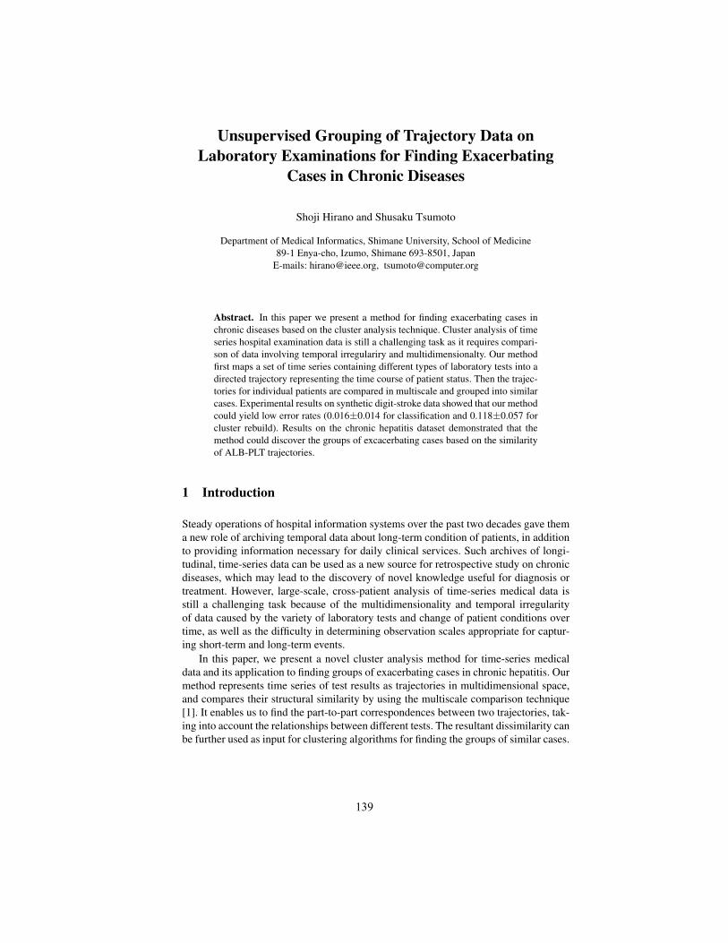
Unsupervised Grouping of Trajectory Data onLaboratory Examinations for Finding Exacerbating

Cases in Chronic Diseases

Shoji Hirano and Shusaku Tsumoto

Department of Medical Informatics, Shimane University, School of Medicine89-1 Enya-cho, Izumo, Shimane 693-8501, Japan

E-mails: hirano@ieee.org, tsumoto@computer.org

Abstract. In this paper we present a method for finding exacerbating cases inchronic diseases based on the cluster analysis technique. Cluster analysis of timeseries hospital examination data is still a challenging task as it requires compari-son of data involving temporal irregulariry and multidimensionalty. Our methodfirst maps a set of time series containing different types of laboratory tests into adirected trajectory representing the time course of patient status. Then the trajec-tories for individual patients are compared in multiscale and grouped into similarcases. Experimental results on synthetic digit-stroke data showed that our methodcould yield low error rates (0.016±0.014 for classification and 0.118±0.057 forcluster rebuild). Results on the chronic hepatitis dataset demonstrated that themethod could discover the groups of excacerbating cases based on the similarityof ALB-PLT trajectories.

1 Introduction

Steady operations of hospital information systems over the past two decades gave thema new role of archiving temporal data about long-term condition of patients, in additionto providing information necessary for daily clinical services. Such archives of longi-tudinal, time-series data can be used as a new source for retrospective study on chronicdiseases, which may lead to the discovery of novel knowledge useful for diagnosis ortreatment. However, large-scale, cross-patient analysis of time-series medical data isstill a challenging task because of the multidimensionality and temporal irregularityof data caused by the variety of laboratory tests and change of patient conditions overtime, as well as the difficulty in determining observation scales appropriate for captur-ing short-term and long-term events.

In this paper, we present a novel cluster analysis method for time-series medicaldata and its application to finding groups of exacerbating cases in chronic hepatitis. Ourmethod represents time series of test results as trajectories in multidimensional space,and compares their structural similarity by using the multiscale comparison technique[1]. It enables us to find the part-to-part correspondences between two trajectories, tak-ing into account the relationships between different tests. The resultant dissimilarity canbe further used as input for clustering algorithms for finding the groups of similar cases.

139

In the experiments we demonstrate the usefulness of our approach through the group-ing tasks of artificially generated digit stroke trajectories and medical test trajectorieson chronic hepatitis patients.

The main contributions of our method are twofold. First, it proposes a new ap-proach to comparing trajectories of medical data by shape comparison techniques, notby standard time-series analysis techniques. Second, it introduces a two-step methodfor deriving dissimilarity between trajectories; multiscale matching is firstly applied inorder to find structurally similar parts, and after that value-based dissimilarity is de-rived for each of the matched pairs and accumulated as the final dissimilarity betweentrajectories. This scheme makes the dissimilarity more informative as it takes not onlyvalue-based features but also structural features into account.

2 Comparison of Trajectories

2.1 Trajectory Representation of Time Series

Let us assume that each patient received M types of hospital laboratory examinations.Each of the M examinations constitutes time series; thus we represent it as exm(t),where m ∈ M . Then the M -dimensional trajectory of examination results, c(t), isrepresented by

c(t) = {ex1(t), ex2(t), . . . , exM (t)}Next, let us denote an observation scale by σ. Then the time-series of the m-th exami-nation at scale σ, EXm(t, σ) is derived by convoluting exm(t) with a smoothing kernelg(t, σ) as follows.

EXm(t, σ) = exm(t)⊗ g(t, σ)

The sampled Gaussian kernel is a general choice for the smoothing kernel; however,according to Lindeberg [2], the use of modified Bessel function is more appropriate fordiscrete time series because the sampled Gaussian may lose some of the desirable prop-erties that a continuous Gaussian has, for example, non-creation of local extrema withthe increase of scale. Using the modified Bessel function, EXm(t, σ) can be derived asfollows.

EXm(t, σ) =∞∑

n=−∞e−σIn(σ)exm(t− n)

where In(σ) denotes the modified Bessel function of order n. The first- and second-order derivatives of EXm(t, σ) are derived as follows.

EX′m(t, σ) =

∞∑n=−∞

−n

σe−σIn(σ)exm(t− n)

EX′′m(t, σ) =

∞∑n=−∞

1σ

(n2

σ− 1)e−σIn(σ)exm(t− n)

140

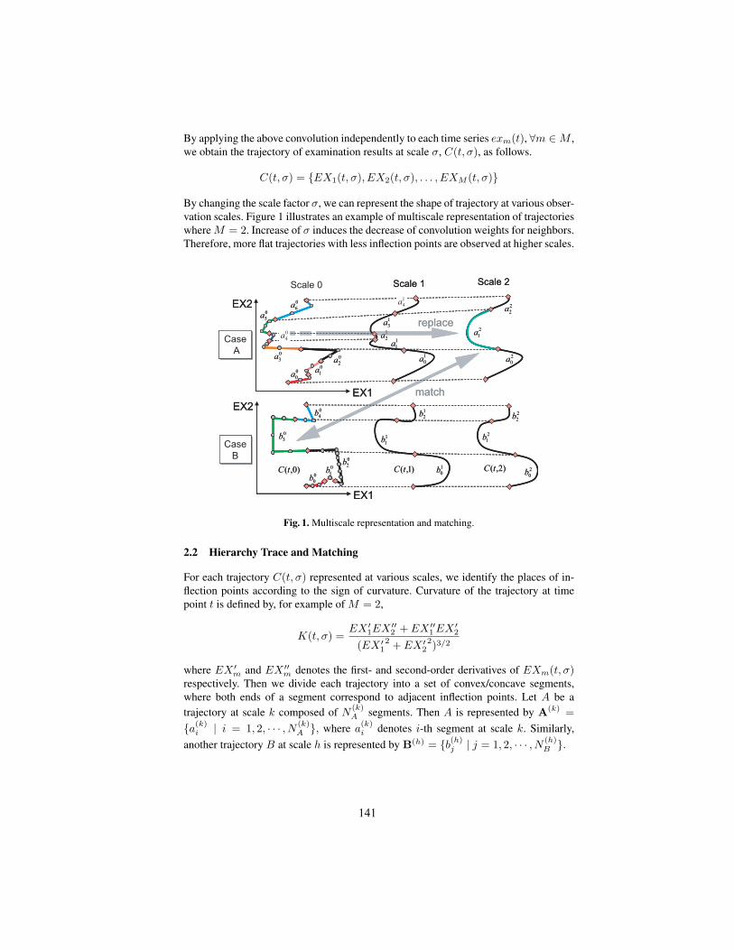
By applying the above convolution independently to each time series exm(t), ∀m ∈ M ,we obtain the trajectory of examination results at scale σ, C(t, σ), as follows.

C(t, σ) = {EX1(t, σ), EX2(t, σ), . . . , EXM (t, σ)}

By changing the scale factor σ, we can represent the shape of trajectory at various obser-vation scales. Figure 1 illustrates an example of multiscale representation of trajectorieswhere M = 2. Increase of σ induces the decrease of convolution weights for neighbors.Therefore, more flat trajectories with less inflection points are observed at higher scales.

Case

B

Case

B

Case

A

Case

A

EX1

EX2

EX1

EX2

0

0b

0

1b

0

2b

0

3b

0

4b1

2b

1

1b

1

0b2

0b

2

1b

2

2b

Scale 0

0

0a

0

1a

0

2a0

3a

0

4a

0

5a

0

6a

Scale 1

1

2a 1

1a

1

0a

1

3a

1

4a

Scale 2

2

0a

2

1a

2

2a

replace

match

)0,(tC )1,(tC )2,(tC

Case

B

Case

B

Case

A

Case

A

EX1

EX2

EX1

EX2

0

0b

0

1b

0

2b

0

3b

0

4b1

2b

1

1b

1

0b2

0b

2

1b

2

2b

Scale 0

0

0a

0

1a

0

2a0

3a

0

4a

0

5a

0

6a

Scale 1

1

2a 1

1a

1

0a

1

3a

1

4a

Scale 2

2

0a

2

1a

2

2a

replace

match

)0,(tC )1,(tC )2,(tC

Fig. 1. Multiscale representation and matching.

2.2 Hierarchy Trace and Matching

For each trajectory C(t, σ) represented at various scales, we identify the places of in-flection points according to the sign of curvature. Curvature of the trajectory at timepoint t is defined by, for example of M = 2,

K(t, σ) =EX ′

1EX ′′2 + EX ′′

1 EX ′2

(EX ′12 + EX ′

22)3/2

where EX ′m and EX ′′

m denotes the first- and second-order derivatives of EXm(t, σ)respectively. Then we divide each trajectory into a set of convex/concave segments,where both ends of a segment correspond to adjacent inflection points. Let A be atrajectory at scale k composed of N

(k)A segments. Then A is represented by A(k) =

{a(k)i | i = 1, 2, · · · , N (k)

A }, where a(k)i denotes i-th segment at scale k. Similarly,

another trajectory B at scale h is represented by B(h) = {b(h)j | j = 1, 2, · · · , N (h)

B }.

141

Next, we chase the cross-scale correspondence of inflection points from top scalesto bottom scale. It defines the hierarchy of segments and guarantees the connectivity ofsegments at different scales. Details of the algorithm for checking segment hierarchy isavailable in ref. [1]. In order to apply the algorithm for closed curve to open trajectory,we modified it to allow replacement of odd number of segments at sequence ends, sincecyclic property of a set of inflection points can be lost.

The main procedure of multiscale matching is to search the best set of segment pairsthat satisfies both of the following conditions:

1. Complete Match: By concatenating all segments, the original trajectory must becompletely formed without any gaps or overlaps.

2. Minimal Difference: The sum of segment dissimilarities over all segment pairsshould be minimized.

The search is performed throughout all scales. For example, in Figure 1, three con-tiguous segments a

(0)3 − a

(0)5 at the lowest scale of case A can be integrated into one

segment a(2)1 at upper scale 2, and the replaced segment well matches to one segment

b(0)3 of case B at the lowest scale. Thus the set of the three segments a

(0)3 − a

(0)5 and

one segment b(0)3 will be considered as a candidate for corresponding segments. On the

other hand, segments such as a(0)6 and b

(0)4 are similar even at the bottom scale without

any replacement. Therefore they will be also a candidate for corresponding segments.In this way, if segments exhibit short-term similarity, they are matched at a lower scale,and if they present long-term similarity, they are matched at a higher scale.

2.3 Local Segment Difference

In order to evaluate the structural (dis-)similarity of segments, we first describe thestructural feature of a segment by using shape parameters defined below.

1. Gradient at starting point: g(a(k)m )

2. Rotation angle: θ(a(k)m )

3. Velocity: v(a(k)m )

Figure 2 illustrates these parameters. Gradient represents the direction of the trajectoryat the beginning of the segment. Rotation angle represents the amount of change ofdirection along the segment. Velocity represents the speed of change in the segment,which is calculated by dividing segment length by the number of points in the segment.

Next, we define the local dissimilarity of two segments, a(k)m and b

(h)n , as

d(a(k)m , b(h)

n ) =

√(g(a(k)

m )− g(b(h)n )

)2

+(θ(a(k)

m )− θ(b(h)n )

)2

+∣∣∣v(a(k)

m )− v(b(h)n )

∣∣∣ + γ{

cost(a(k)m ) + cost(b(h)

n )}

where cost() denotes a cost function used for suppressing excessive replacement ofsegments, and γ is the weight of costs. We define the cost function using local segment

142

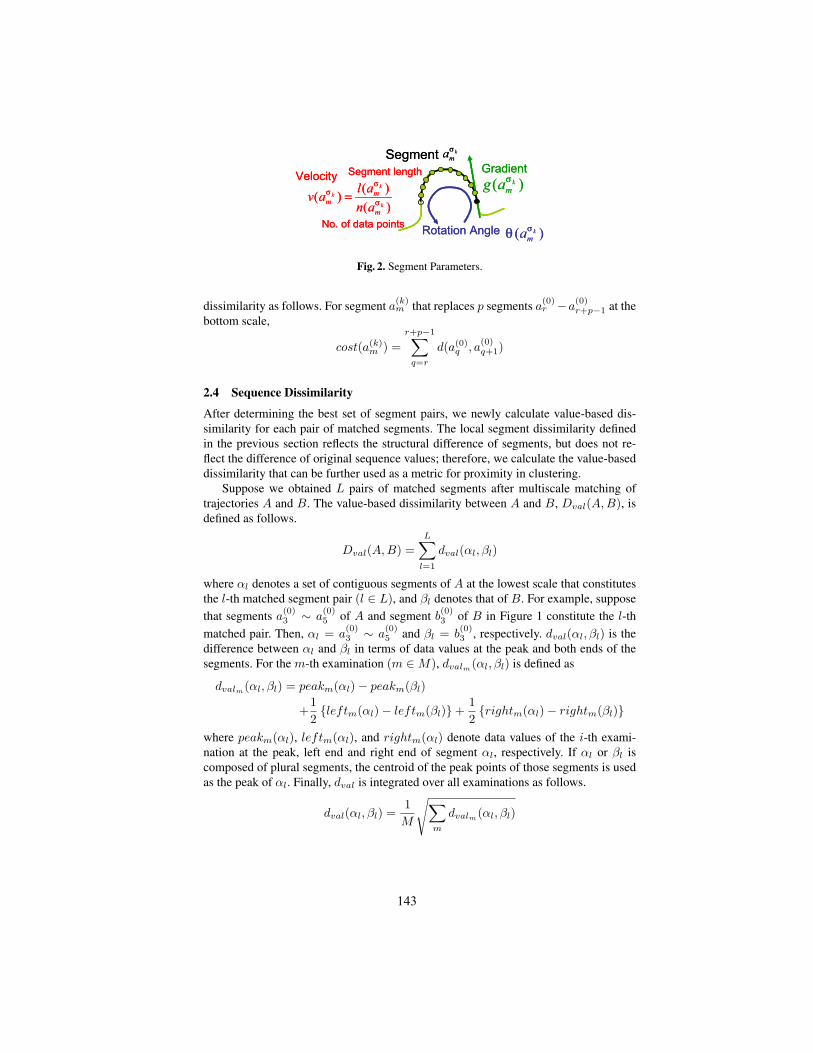
)( k

maσ

θ

)( k

magσ

k

maσ

Segment

)(

)()(

k

k

k

m

mm

an

alav

σ

σ

σ=

Segment length

No. of data pointsRotation Angle

VelocityGradient

)( k

maσ

θ

)( k

magσ

k

maσ

Segment

)(

)()(

k

k

k

m

mm

an

alav

σ

σ

σ=

Segment length

No. of data pointsRotation Angle

VelocityGradient

Fig. 2. Segment Parameters.

dissimilarity as follows. For segment a(k)m that replaces p segments a

(0)r −a

(0)r+p−1 at the

bottom scale,

cost(a(k)m ) =

r+p−1∑q=r

d(a(0)q , a

(0)q+1)

2.4 Sequence Dissimilarity

After determining the best set of segment pairs, we newly calculate value-based dis-similarity for each pair of matched segments. The local segment dissimilarity definedin the previous section reflects the structural difference of segments, but does not re-flect the difference of original sequence values; therefore, we calculate the value-baseddissimilarity that can be further used as a metric for proximity in clustering.

Suppose we obtained L pairs of matched segments after multiscale matching oftrajectories A and B. The value-based dissimilarity between A and B, Dval(A,B), isdefined as follows.

Dval(A,B) =L∑

l=1

dval(αl, βl)

where αl denotes a set of contiguous segments of A at the lowest scale that constitutesthe l-th matched segment pair (l ∈ L), and βl denotes that of B. For example, supposethat segments a

(0)3 ∼ a

(0)5 of A and segment b

(0)3 of B in Figure 1 constitute the l-th

matched pair. Then, αl = a(0)3 ∼ a

(0)5 and βl = b

(0)3 , respectively. dval(αl, βl) is the

difference between αl and βl in terms of data values at the peak and both ends of thesegments. For the m-th examination (m ∈ M), dvalm(αl, βl) is defined as

dvalm(αl, βl) = peakm(αl)− peakm(βl)

+12{leftm(αl)− leftm(βl)}+

12{rightm(αl)− rightm(βl)}

where peakm(αl), leftm(αl), and rightm(αl) denote data values of the i-th exami-nation at the peak, left end and right end of segment αl, respectively. If αl or βl iscomposed of plural segments, the centroid of the peak points of those segments is usedas the peak of αl. Finally, dval is integrated over all examinations as follows.

dval(αl, βl) =1M

√∑m

dvalm(αl, βl)

143

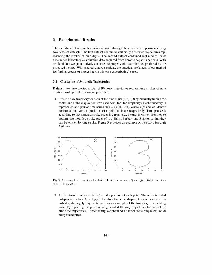
3 Experimental Results

The usefulness of our method was evaluated through the clustering experiments usingtwo types of datasets. The first dataset contained artificially generated trajectories rep-resenting the strokes of nine digits. The second dataset contained real medical data;time series laboratory examination data acquired from chronic hepatitis patients. Withartificial data we quantitatively evaluate the property of dissimilarities produced by theproposed method. With medical data we evaluate the practical usefulness of our methodfor finding groups of interesting (in this case exacerbating) cases.

3.1 Clustering of Synthetic Trajectories

Dataset We have created a total of 90 noisy trajectories representing strokes of ninedigits according to the following procedure.

1. Create a base trajectory for each of the nine digits (1,2,...,9) by manually tracing thecenter line of the display font (we used Arial font for simplicity). Each trajectory isrepresented as a pair of time series c(t) = (x(t), y(t)), where x(t) and y(t) denotehorizontal and vertical positions of a point at time t respectively. Time proceedsaccording to the standard stroke order in Japan; e.g., 1 (one) is written from top tobottom. We modified stroke order of two digits, 4 (four) and 5 (five), so that theycan be written by one stroke. Figure 3 provides an example of trajectory for digit3 (three).

0

5

10

15

20

25

30

35

0 10 20 30 40 50 60 70 80

Poi

nt L

ocat

ion

Time t

x(t)y(t)

5

10

15

20

25

30

35

5 10 15 20 25 30 35

Loca

tion

y

Location x

c(t)

Fig. 3. An example of trajectory for digit 3. Left: time series x(t) and y(t). Right: trajectoryc(t) = (x(t), y(t)).

2. Add a Gaussian noise ∼ N(0, 1) to the position of each point. The noise is addedindependently to x(t) and y(t); therefore the local shapes of trajectories are dis-turbed quite largely. Figure 4 provides an example of the trajectory after addingnoise. By repeating this process, we generated 10 noisy trajectories for each of thenine base trajectories. Consequently, we obtained a dataset containing a total of 90noisy trajectories.

144

0

5

10

15

20

25

30

35

0 10 20 30 40 50 60 70 80

Poi

nt L

ocat

ion

Time t

x(t)y(t)

5

10

15

20

25

30

35

5 10 15 20 25 30 35

Loca

tion

y

Location x

c(t)

Fig. 4. An example of trajectory after adding noise to Figure 3.

Classification First, we tested whether the proposed method could produce the dissim-ilarities that can be used for classification of trajectories. A pseudo 1-NN classificationexperiment was conducted and classification error was evaluated according to the fol-lowing procedure.

1. Perform pair-wise comparison of 90 trajectories using the proposed method andconstruct a 90×90 dissimilarity matrix.

2. Select one case, and classify it into the class of the nearest object.3. Repeat the select/classify step for each of 90 cases and calculate the classification

error

We have repeated the above test 100 times using different (disjoint) sets of trajectories.The error ratio was 0.016 ± 0.014 (mean ± SD), which means > 98% of trajectorieswere classified correctly using the dissimilarities produced by the proposed method.

Cluster Rebuild Next, we tested whether the dissimilarities can be used to correctlyform the original structure of the data. The procedure was as follows: (1) using the90×90 dissimilarity matrix, rebuild clusters fixing the cluster number=9. and (2) eval-uate the grouping error ratio with regard to digit labels determined by voting. We usedgroup average hierarchical clustering [3] as the grouping method. Similarly to clas-sification experiment, this procedure was repeated 100 times using different sets oftrajectories.

The error ratio was 0.118 ± 0.057, which means about 88% of trajectories weregrouped correctly. Figure 5 shows an example of the dendrogram that resulted in in-correct grouping. The horizontal line shows cutting level for nine clusters. The notionsc1, c2, . . . , c9 represent the cluster number respectively. The notions 6, 8, . . . , 1 at thebottom of the dendrogram represent correct groups, namely, labels of digits that thetrajectories should represent.

Each of the clusters except for c3, c7 and c8 contained 10 trajectories that correctlyrepresented the same digit. Cluster c3 contained a total of 20 trajectories, half repre-senting digit 5 (five) and the remaining half representing 9 (nine). Figure 5 providesthe first 16 of trajectories in c3. The stroke of 9 (nine) starts from the junction at cen-ter right. The stroke of 5 (five) should start from upper left, however, we modified its

145

c1 c2 c3 c4 c5 c6c7 c8

c9

98 76 5 4 3 2 1

c1 c2 c3 c4 c5 c6c7 c8

c9

98 76 5 4 3 2 1

Fig. 5. Left: An example of dendrogram resulted in incorrect grouping. Right: Trajectories incluster 3.

stroke order to start from upper right so that it could be written in one stroke. As aresult, the base trajectories for these two digits look very similar. They were groupedinto the same cluster under this nine clusters solution, however, the dendrogram showsthey could be separated correctly at relatively low values of dissimilarity. Trajectoriesrepresenting the digit 7 (seven) were separated into two clusters, c7 with 1 case, and c8

with remaining 9 cases, though they could be merged at the next step. This seemed tooccur because the method failed to find the good match for the one case in c7 under thegiven parameters.

3.2 Clustering of Trajectories of Medical Data

Data and Procedure of Experiments We applied our method to the chronic hepatitisdataset which was a common dataset in ECML/PKDD discovery challenge 2002-2004.The dataset contained time series laboratory examinations data collected from 771 pa-tients of chronic hepatitis B and C. According to the previous study conducted by Hi-rano et al. [4], we focused on the analysis about temporal relationships between albumin(ALB) and platelet count (PLT), and their relation to fibrotic stages. The subjects were99 cases of Type C viral hepatitis who did not receive the interferon (IFN) treatment.

We performed cluster analysis on ALB-PLT trajectories according to the followingprocedure. (1) Select a pair of cases (patients) and calculate the dissimilarity by usingthe proposed method. (2) Apply this procedure for all pairs of cases and construct a dis-similarity matrix. (3) Create a dendrogram by using conventional hierarchical clustering[3] and the dissimilarity matrix. Then perform cluster analysis.

3.3 Results

Figure 6 left shows the dendrogram generated from ALB-PLT trajectories. The overallshape of the dendrogram implied the existence of a few major clusters; however, in or-der to carefully examine the data structure, we here avoided excessive merge of clusters

146

17 clusters solution

1 177 8

Progressed Un-progressed

17 clusters solution

1 177 8

Progressed Un-progressed

Fig. 6. Left: Dendrogram. Right: Cluster constitutions w.r.t. fibrotic stages (Small clusters of N <2 omitted.)

and determined to split it into 17 clusters where dissimilarity increased relatively largeat early stage. For each of the 8 clusters that contained ≥ 2 cases, we classified casesaccording to the fibrotic stage. Figure 6 right shows the summary. The leftmost col-umn shows cluster number. The next column shows the number of cases whose fibroticstages were F0 or F1. The subsequent three columns show the number of F2, F3, andF4 cases respectively. The rightmost column shows the total number of cases in eachcluster. Globally, it could be recognized that clusters can be classified into one of thetwo categories: one containing progressed cases of liver fibrosis (clusters 5 and 7) andanother containing un-progressed cases (clusters 9, 11, 14, 15, 16 and 17). This impliedthat the difference about ALB and PLT might be related to the fibrotic stages.

Figures 7 and 8 show the examples of grouped ALB-PLT trajectories. Each quadrateregion contains a trajectory of ALB-PLT values for a patient. If the number of casesin a cluster was larger than 16, the first 16 cases w.r.t. ID number were selected forvisualization. The bottom part of Figure 7 provides the legend. The horizontal axisrepresents ALB value, and the vertical axis represents PLT value. Lower end of thenormal range (ALB:3.9g/dl, PLT:120 × 103/ul) and Upper end of the normal range(ALB:5.0g/dl, PLT:350 × 103/ul) were marked with blue and red short lines on eachaxis respectively. Time phase on each trajectory was represented by color phase: redrepresents the start of examination, and it changes toward blue as time proceeds.

Figure 7 shows cases grouped into cluster 5 which contained remarkably many F4cases (3/4). The skewed trajectory of ALT and PLT clearly demonstrated that both val-ues decreased from the normal range to the lower range as time proceeded, due to thedysfunction of the liver, as observed in the exacerbating cases. Cluster 7, shown in Fig-ure 8 left, also contained similarly large number of progressed cases (F4:9/16, F3:2/16)and exhibited the similar characteristics, though it was relatively weaker than in cluster5. On the contrary, clusters that contained many un-progressed cases exhibited differentcharacteristics. Figure 8 right shows the trajectories grouped into cluster 17, where the

147

Cluster 5: N=4 (0/1/0/3)

ALB

PLT

t=0

t=T

Upper Normal(350 x103/ul)

Lower Normal(120 x103/ul)

Upper Normal(5.0 g/dl)

Lower Normal(3.9 g/dl)

<Legend>

Cluster 5: N=4 (0/1/0/3)

ALB

PLT

t=0

t=T

Upper Normal(350 x103/ul)

Lower Normal(120 x103/ul)

Upper Normal(5.0 g/dl)

Lower Normal(3.9 g/dl)

<Legend>

Fig. 7. Trajectories in Cluster 5.

Cluster 7: N=16 (3/2/2/9)Cluster 7: N=16 (3/2/2/9) Cluster 17: N=23 (20/2/1/0)Cluster 17: N=23 (20/2/1/0)

Fig. 8. Left: Trajectories in Cluster 7. Right Trajectories in Cluster 17.

number of F0/F1 cases was large (20/23). Most of the trajectories moved within thenormal range, and no clear feature about time-direction dependency was observed.

The above observation suggested the existence of two major classes on the dendro-gram: progressed cases and un-progressed cases. In order to confirm this hypothesis, wehave investigated the number of cases that reached abnormally low PLT level. As PLTlevel is considered to correlate with fibrotic stage [5], its decrease to the abnormally lowlevel would imply that liver fibrosis progressed to F4. The judgment of reaching F4 wasbased on the following assumption [4] : “If the PLT level of a patient is continuouslylower than the normal range for at least 6 months, and after that never keeps normalrange more than 6 months, then the patient is F4.”

Table 1 provides the results. The left subtable summarizes the results for clusters1-7, which were grouped into the left branch on the dendrogram in Figure 6. The rightsubtable are those for cluster 8-17, which were grouped into the right branch of the

148

Table 1. Comparison of clusters w.r.t. the number of cases that reached abnormally low PLT level

Cluster Number of CasesReached Total

1 0 12 1 13 1 14 0 15 4 46 1 17 12 16

Total 19 25

Cluster Number of CasesReached Total

8 0 19 0 8

10 0 111 0 712 0 113 1 114 2 315 4 2716 0 217 0 23

Total 7 74

dendrogram. It can be clearly observed that the ratio of cases that reached abnormallylow PLT level was remarkably higher in the left cluster (19/25) than in the right cluster(7/74). This demonstrated that the proposed method could discover the interesting fea-ture of ALB-PLT trajectories; there might exist two major categories representing pro-gressed cases and un-progressed cases, and the trajectories of progressed cases mighttake the skewed shapes representing their exacerbating patterns.

4 Conclusions

In this paper, we have presented a novel cluster analysis method for time-series medicaldata and its application to finding groups of exacerbating cases in chronic hepatitis. Ourmethod employed a two-stage approach. Firstly, it compared two trajectories based ontheir structural similarity, and determines the best correspondence of partial trajecto-ries. After that, it calculated the value-based dissimilarity for the all pairs of matchedsegments, and outputs the total sum as dissimilarity of the two trajectories.

Experimental results on digit stroke data showed that the method could produce dis-similarities that can be used for classification/clustering of trajectories. Experiments onchronic hepatitis data showed that the method could discover the groups of exacerbatingcases based on the trajectories of ALB-PLT. Although further examination is needed,the results may open a new way to knowledge discovery in medical data, that is, the useof data-driven, time-series clustering results as a new decision class for rule discovery.

Our future work include the clinical validation of the results, treatment of the highdimensional data, and refinement of segment parameters.

Acknowledgments

This work was supported in part by the Grant-in-Aid for Scientific Research on PriorityArea “Knowledge Discovery from Multidimensional Trajectory Data and Its Appli-cation to Medicine” (#19024060) by the Ministry of Education, Culture, Science andTechnology of Japan.

149

References

1. N. Ueda and S. Suzuki (1990): A Matching Algorithm of Deformed Planar Curves UsingMultiscale Convex/Concave Structures. IEICE Transactions on Information and Systems, J73-D-II(7): 992–1000.

2. T. Lindeberg (1990): Scale-Space for Discrete Signals. IEEE Trans. PAMI, 12(3):234–254.3. B. S. Everitt, S. Landau, and M. Leese (2001): Cluster Analysis Fourth Edition. Arnold Pub-

lishers.4. S. Tsumoto, S. Hirano, and K. Takabayashi (2005): Development of the Active Mining Sys-

tem in Medicine Based on Rough Sets. Journal of Japan Society of Artificial Intelligence20(3):203-210.

5. H. Matsumura and M. Moriyama and I. Goto and N. Tanaka, and H. Okubo and Y. Arakawa(2000): Natural course of progression of liver fibrosis in patients with chronic liver diseasetype C in Japan - a study of 527 patients at one establishment in Japan. J. Viral Hepat. 7:375–381.

150

Improving Boosting by exploiting formerassumptions

Emna Bahri, Nicolas Nicoloyannis, andMondher Maddouri

Laboratoire Eric, University Lyon 2.5 avenue Pierre Mendes France, 69676 Bron Cedex{e.bahri,nicolas.nicoloyannis}@univ-lyon2.fr

mondher.maddouri@fst.rnu.tn

http://eric.univ-lyon2.fr

Abstract. The error reduction in generalization is one of the princi-pal motivations of research in machine learning. Thus, a great numberof work is carried out on the classifiers aggregation methods in orderto improve generally, by voting techniques, the performance of a singleclassifier. Among these methods of aggregation, we find the Boostingwhich is most practical thanks to the adaptive update of the distribu-tion of the examples aiming at increasing in an exponential way theweight of the badly classified examples. However, this method is blamedbecause of overfitting, and the convergence speed especially with noise.In this study, we propose a new approach and modifications carried outon the algorithm of AdaBoost. We will demonstrate that it is possibleto improve the performance of the Boosting, by exploiting assumptionsgenerated with the former iterations to correct the weights of the ex-amples. An experimental study shows the interest of this new approach,called hybrid approach.

Key words: Machine learning, Data mining, Classification, Boosting,Recall, convergence

1 Introduction

The great emergence of the modern databases and their evolution in an expo-nential way as well as the evolution of transmission systems result in a hugemass of data which exceeds the human processing and understanding capabili-ties. Certainly, these data are sources of relevant information and require meansof synthesis and interpretation. As a result, researches were based on powerfulsystems of artificial intelligence allowing the extraction of useful informationhelping us in decisions making. Responding to this need, data mining was born.It drew its tools from the statistics and databases. The methodology of datamining gives the possibility to build a model of prediction. This model is a phe-nomenon starting from other phenomena more easily accessible, based on theprocess of the knowledge discovery from data which is a process of intelligent

151

data classification. However, the built model can sometimes generate errors ofclassification that even a random classification does not make. To reduce theseerrors, a great amount of research in data mining and specifically in machinelearning has been carried out on classifiers aggregation methods having as goalto improve by voting techniques the performance of a single classifier. Theseaggregation methods are good for compromised Skew-variance, thanks to thethree fundamental reasons explained in [6]. These methods of aggregation aredivided into two categories. The first category refers to those which merge presetclassifiers, such as simple voting [2], the weighted voting [2], and the weightedmajority voting [13]. The second category consists of those which merge classi-fiers according to data during the training, such as adaptive strategies (Boosting)and the basic algorithm AdaBoost [22] or random strategies (Bagging) [3].We are interested in the method of Boosting, because of the comparative study[7] that shows, in little noise, AdaBoost is seemed to be working against theoverfitting. In fact, AdaBoost tries to optimize directly the weighted votes. Thisobservation has been proved not only by the fact that the empirical error on thetraining set decreases exponentially with iterations, but also by the fact that theerror in generalization also decreases, even when the empirical error reached itsminimum. However, this method is blamed because of overfitting, and the speedof convergence especially with noise. In the last decade, many studies focusedon the weaknesses of AdaBoost and proposed its improvement. The importantimprovements were carried on the modification of the weight of examples [20],[19], [1], [21], [15], [9], the modification of the margin [10], [21], [18],the modification of the classifiers’ weight [16], the choice of weak learning [5],[25] and the speed of convergence [23], [14], [19]. In this paper, we proposea new improvement to the basic Boosting algorithm AdaBoost. This approachaims exploiting assumptions generated with the former iterations of AdaBoostto act both on the modification of the weight of examples and the modificationof the classifiers’ weight. By exploiting these former assumptions, we think thatwe will avoid the re-generation of a same classifier within different iterationsof AdaBoost. Thus, consequently, we expect a positive effect on the improve-ment of the speed of convergence. The paper is organized in three sections. Inthe following section, we describe the studies whose purpose is to improve theBoosting against its weaknesses. In the third section, we describe our improve-ment of boosting by exploiting former assumptions. In the fourth section, wepresent an experimental study of the proposed improvement by comparing itserror in generalization, its recall and its speed of convergence with AdaBoost,on many real databases. We study also the behavior of the proposed improve-ment on noisy data. We present also comparative experiments of our proposedmethod with BrownBoost (a new method known that it improves AdaBoost M1with noisy data). Lastly, we give our conclusions and perspectives.

152

2 State of art

Due to the finding of some weaknesses, such as the overfitting and the speedof convergence, met by the basic algorithm of boosting AdaBoost, several re-searchers have tried to improve it. Therefore , we make a study of main methodshaving as purpose to improve boosting relatively to these weaknesses. With thisintention, the researchers try to use the strong points of Boosting such as theupdate of the badly classified examples, the maximization of the margin, thesignificance of the weights that AdaBoost associates the hypothesis and finallythe choice of weak learning.

2.1 Modification of the examples’ weight:

The distributional adaptive update of the examples, aiming at increasing theweight of those badly learned by the preceding classifier, makes it possible toimprove the performance of any training algorithm . Indeed, with each iteration,the current distribution supports the examples having been badly classified bythe preceding hypothesis, which characterizes the adaptivity of AdaBoost. As aresult, several researchers proposed strategies related to a modification of weightupdate of the examples, to avoid the overfitting.Indeed, we can quote for example MadaBoost [9] whose aim is to limit theweight of each example by its initial probability. It acts thus on the uncontrolledgrowth of the weight of certain examples (noise) which is the problem of over-fitting.Another approach which make the algorithm of boosting resistant to the noiseis Brownboost [15], an algorithm based on Boost-by-Majority by incorporatinga time parameter. Thus for an appropriate value of this parameter, BrownBoostis able to avoid the overfitting. Another approach, which adapts to AdaBoost alogistic regression model, is Logitboost [19].An approach, which produces less errors of generalization compared with the tra-ditional approach but with the cost of an error of training slightly more raised ,is the Modest boost [1]. In fact, its update is based on the reduction in the con-tribution of classifier, if that functions ”too well” on the data correctly classified.This is why the method is called Modest AdaBoost - it forces the classifiers tobe ”modest” and it works only in the field defined by a distribution.An approach, which tries to reduce the effect of overfitting by imposing limi-tations on the distribution produced during the process of boosting is used inSmoothBoost [21]. In particular, a limited weight is assigned to each exampleindividually during each iteration. Thus, the noisy data can be excessively un-derlined during the iterations since they are assigned to the extremely largeweights.A last approach, Iadaboost [20], is based on the idea of building around eachexample a local information measurement, making it possible to evaluate theoverfitting risks, by using neighboring graph to measure information around eachexample. Thanks to these measurements, we have a function which translates

153

the need for updating the example. This function makes it possible to managethe outliers and the centers of clusters at the same time.

2.2 Modification of the margin:

Certain studies, analyzing the behavior of Boosting, showed that the error ingeneralization still decreases even when the errors in training are stable. Theexplanation is that even if all the examples of training are already well classified,Boosting tends to maximize the margins [21].Following this, some studies try to modify the margin either by maximizing itor by minimizing it with the objective of improving the performance of Boostingagainst overfitting.Several approaches followed such as AdaBoostReg [18] which tries to identifyand remove badly labeled examples, or to apply the constraint of the maximummargin to examples supposed to be badly labeled, by using the Soft Margin.In the algorithm, proposed by [10], the authors use a weighting diagram whichexploits a margin function that grows less quickly than the exponential function.

2.3 Modification of the classifiers’ weight:

During the performance evaluation of Boosting, researchers wondered about thesignificance of the weights α(t) that AdaBoost associates with the producedhypotheses.However, they noted at the time of experiments on very simple data that theerror in generalization decreased further whereas the weak learning had alreadyprovided all the possible hypotheses. In other words, when a hypothesis appearsseveral times, it votes finally with a weight, office sum of all α(t), which isperhaps absolute. So several researchers hoped to approach these values by anonadaptive process , such as locboost [16] an alternative to the construction ofthe whole representations of experts which allows the coefficients α(t) to dependon the data.

2.4 Choice of weak learner :

A question that several researchers posed against the problems of boosting isthat of weak learner and how to make a good choice of this classifier?A lot of research moves towards the study of choosing the basic classifier ofboosting, such as GloBoost [25]. This approach use a weak learner which pro-duces only correct hypotheses. RankBoost [5] is also an approach which is basedon weak learner which accepts as data attributes functions of rank.

2.5 The speed of convergence

In addition to the problem of overfitting met by boosting in the modern databasesmentioned above, we find another problem : the speed of convergence of Boost-ing especially AdaBoost.

154

Indeed, in the presence of noisy data, the optimal error of the training algorithmused is reached after a long time. In other words, AdaBoost ”loses” iterations,and thus time, with reweighing examples which do not deserve in theory anyattention, since it is a noise.Thus research was made to detect these examples and improve the performanceof Boosting in terms of convergence such as: iBoost [23] which aims at special-izing weak hypotheses on the examples supposed to be correctly classified.The IAdaBoost approach also contributes to improve AdaBoost against its speedof convergence. In fact, the basic idea of the improvement is the modification ofthe theorem [19]. This modification is carried out in order to integrate the riskof Bayes. The effects of this modification are a faster convergence towards theoptimal risk and a reduction of the number of weak hypotheses to build. Finally,RegionBoost [14] is a new weighting strategy of each classifier. This weightingis evaluated at the voting time by a technique based on K Nearest Neighbors ofthe example to label. This approach makes it possible to specialize each classifieron areas of the training data.

3 Boosting by exploiting former assumptions

To improve the performance of AdaBoost and to avoid forcing it to learn eitherfrom the examples that contain noise, or from the examples which would becometoo difficult to learn during the process of Boosting, we propose a new approach.This approach is based on the fact that for each iteration, Adaboost, buildshypotheses on a defined sample, it makes its updates and it calculates the errorof training according to the results given only by these hypotheses. In addition,it does not exploit the results provided by the hypotheses already built on othersamples to the former iterations. This approach is called AdaBoostHyb

Program Code Input X0 to classify , S = (x1, y1), ....., (xn, yn) Sample

– For i=1,n Do– p0(xi) = 1/n;– End FOR– t← 0– While t ≤ T Do– Learning sample St from S with probabilities pt.– Build a hypotheses ht on St with weak learning A.– εt apparent error of ht on S with εt =

∑weight of examples

such that argmax(∑t

i=1 αihi(xi) 6= yi). αt = 1/2ln((1− εt)/εt).– For i=1, m Do– Pt+1(xi) ← (pt(xi)/Zt)e−αt if argmax(

∑ti=1 αihi(xi)) = yi (correctly

classifiedPt+1(xi) ← (pt(xi)/Zt)e+αt if argmax(

∑ti=1 αihi(xi)) 6= yi (badly

classified(Zt normalized to

∑ni=1 pt(xi) = 1)

155

– End Fort← t + 1

– End While– Final hypotheses :

H(x) = argmax y ∈ Y∑T

t=1 αt

The modification within the algorithm is made

During the modification of the weights of the examples: Indeed, this strategy,with each iteration, is based on the opinion of the experts already used (hypothe-ses of the former iterations) for the update of the weight of the examples.In fact, we do not compare only the class predicted by the hypothesis of thecurrent iteration with the real class but also the sum of the hypotheses balancedfrom the first iteration to the current iteration. If this sum votes for a class dif-ferent from the real class, an exponential update such as in the case of AdaBoostis applied to the badly classified example. Thus, this modification lets the algo-rithm be interested only in the examples which are either badly classified or notclassified yet. So, results related to the improvement the speed of convergenceare awaited, similarly for the reduction of the error of generalization , becauseof the richness of the space of hypotheses to each iteration.During the error analysis ε(t) of the hypothesis to the iteration T: Indeed, thisother strategy is rather interested in the classifiers’ coefficient ( hypothesis) toeach iteration α(t).In fact, this coefficient depends on the apparent error analysis ε(t). This method,with each iteration, takes into account hypotheses preceding the current itera-tion during the calculation of ε(t). So the apparent error with each iteration isthe weight of the examples voted badly classified by the hypotheses weighted ofthe former iterations by comparison to the real class .Results in improving the error of generalization are expected since the vote ofeach hypothesis (coefficient α(t)) is calculated from the other hypotheses.

4 Experiments

The objective of this part is to compare our new approach and especially itscontribution with the original approach of Adaboost and to look further intothis comparison by the choice of a version improved of Adaboost (BrownBoost[15]).Our Choice of BrownBoost was based on its robustness against the problems ofnoisy data. In fact,BrownBoost is an adaptive algorithm which incorporates atime parameter that corresponds to the proportion of noise in the training data.So by a good estimation of this parameter BrownBoost is capable of avoidingoverfitting. The comparison criterions chosen in this article are the error rate,the recall, the speed of convergence and the sensitivity to noise.

To do this experimental comparison, we used the C4.5 algorithm as a weaklearner (according to the study of Dietterich [6]). To estimate without skew

156

the theoretical success rate, we used a procedure of cross-validation in 10 folds(according to the study [12]). In order to choose the databases for our experi-ments, we considered the principle of diversity . We have considered 15 databasesof the UCI [8]. Some databases are characterized by theirs missing values (NHL,Vote, Hepatitis, Hypothyroid). Some others concern the problem of multi-classprediction (Iris: 3 classes, Diabetes: 4 classes, Zoo: 7 classes, IDS: 12 classes).We choose the IDS database [24] especially because it has 35 attributes. Table1 describes the 15 databases used in the experimental comparison.

Databases Nb. Inst Attrib Cl. Pred Miss.VaLIRIS 150 4 numeric 3 noNHL 137 8 numeric and symbolic 2 yes

VOTE 435 16 boolean valued 2 yesWEATHER 14 4 numeric and symbolic 2 noCREDIT-A 690 16numeric and symbolic 2 yesTITANIC 750 3 symbolic 2 no

DIABETES 768 8 numeric 2 noHYPOTHYROID 3772 30 numeric and symbolic 4 yes

HEPATITIS 155 19 numeric and symbolic 2 yesCONTACT-LENSES 24 4 nominal 3 no

ZOO 101 18 numeric and boolean 7 noSTRAIGHT 320 2 numeric 2 no

IDS 4950 35 numeric and symbolic 12 noLYMPH 148 18 numeric 4 no

BREAST-CANCER 286 9 numeric and symbolic 2 yesTable 1. Databases Description

4.1 Comparison of generalization error

Table 2 indicated the error rates in 10-fold cross-validation corresponding to thealgorithm AdaBoost M1,BrownBoost and the proposed one. We used the samesamples for the tree algorithms in cross-validation for comparison purposes. Theresults are obtained while having chosen for each algorithm to carry out 20iterations. The study of the effect of the number of iterations on the error ratesof the tree algorithms will be presented in the section 4.3, where we will considerabout 100 iterations.

The results in table 2 show already that the proposed modifications improvethe error rates of AdaBoost. Indeed, for 14 databases out of 15, the proposedalgorithm shows an error rate lower or equal to AdaBoost M1. We remark, also,a significant improvement of the error rates corresponding to the three databasesNHL, CONTACT-LENS and BREAST-CANCER. For example, the error ratecorresponding to the BREAST-CANCER database goes from 45.81% to 30.41%.

Even, if we compare the proposed algorithm with BrownBoost, we remarkthat for 11 databases out of 15 the proposed algorithm shows an error rate loweror equal to BrownBoost.

This gain shows that by exploiting hypotheses generated with the formeriterations to correct the weights of the examples, it is possible to improve the

157

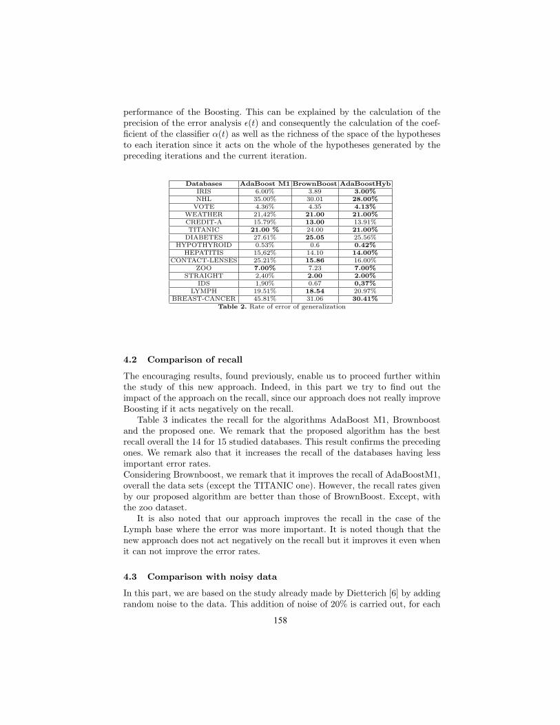
performance of the Boosting. This can be explained by the calculation of theprecision of the error analysis ε(t) and consequently the calculation of the coef-ficient of the classifier α(t) as well as the richness of the space of the hypothesesto each iteration since it acts on the whole of the hypotheses generated by thepreceding iterations and the current iteration.

Databases AdaBoost M1 BrownBoost AdaBoostHybIRIS 6.00% 3.89 3.00%NHL 35.00% 30.01 28.00%

VOTE 4.36% 4.35 4.13%WEATHER 21,42% 21.00 21.00%CREDIT-A 15.79% 13.00 13.91%TITANIC 21.00 % 24.00 21.00%

DIABETES 27.61% 25.05 25.56%HYPOTHYROID 0.53% 0.6 0.42%

HEPATITIS 15,62% 14.10 14.00%CONTACT-LENSES 25.21% 15.86 16.00%

ZOO 7.00% 7.23 7.00%STRAIGHT 2,40% 2.00 2.00%

IDS 1,90% 0.67 0,37%LYMPH 19.51% 18.54 20.97%

BREAST-CANCER 45.81% 31.06 30.41%Table 2. Rate of error of generalization

4.2 Comparison of recall

The encouraging results, found previously, enable us to proceed further withinthe study of this new approach. Indeed, in this part we try to find out theimpact of the approach on the recall, since our approach does not really improveBoosting if it acts negatively on the recall.

Table 3 indicates the recall for the algorithms AdaBoost M1, Brownboostand the proposed one. We remark that the proposed algorithm has the bestrecall overall the 14 for 15 studied databases. This result confirms the precedingones. We remark also that it increases the recall of the databases having lessimportant error rates.Considering Brownboost, we remark that it improves the recall of AdaBoostM1,overall the data sets (except the TITANIC one). However, the recall rates givenby our proposed algorithm are better than those of BrownBoost. Except, withthe zoo dataset.

It is also noted that our approach improves the recall in the case of theLymph base where the error was more important. It is noted though that thenew approach does not act negatively on the recall but it improves it even whenit can not improve the error rates.

4.3 Comparison with noisy data

In this part, we are based on the study already made by Dietterich [6] by addingrandom noise to the data. This addition of noise of 20% is carried out, for each

158

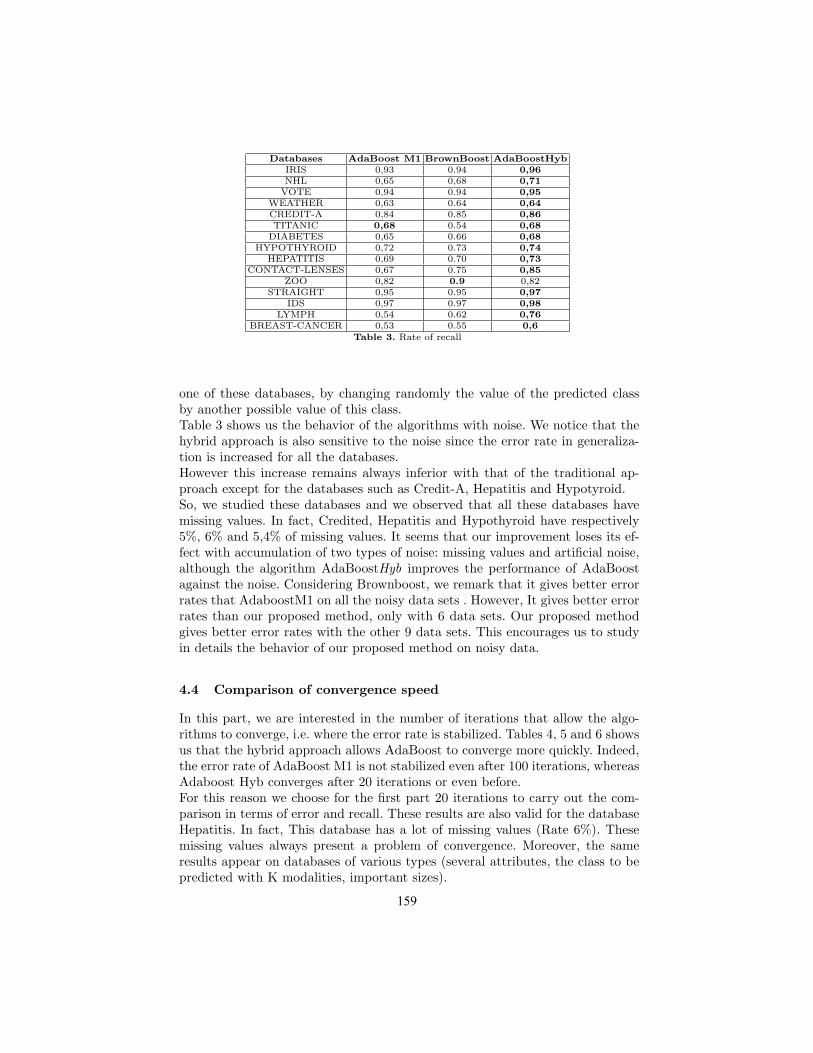
Databases AdaBoost M1 BrownBoost AdaBoostHybIRIS 0,93 0.94 0,96NHL 0,65 0,68 0,71

VOTE 0,94 0.94 0,95WEATHER 0,63 0.64 0,64CREDIT-A 0,84 0.85 0,86TITANIC 0,68 0.54 0,68

DIABETES 0,65 0.66 0,68HYPOTHYROID 0,72 0.73 0,74

HEPATITIS 0,69 0.70 0,73CONTACT-LENSES 0,67 0.75 0,85

ZOO 0,82 0.9 0,82STRAIGHT 0,95 0.95 0,97

IDS 0,97 0.97 0,98LYMPH 0,54 0.62 0,76

BREAST-CANCER 0,53 0.55 0,6Table 3. Rate of recall

one of these databases, by changing randomly the value of the predicted classby another possible value of this class.Table 3 shows us the behavior of the algorithms with noise. We notice that thehybrid approach is also sensitive to the noise since the error rate in generaliza-tion is increased for all the databases.However this increase remains always inferior with that of the traditional ap-proach except for the databases such as Credit-A, Hepatitis and Hypotyroid.So, we studied these databases and we observed that all these databases havemissing values. In fact, Credited, Hepatitis and Hypothyroid have respectively5%, 6% and 5,4% of missing values. It seems that our improvement loses its ef-fect with accumulation of two types of noise: missing values and artificial noise,although the algorithm AdaBoostHyb improves the performance of AdaBoostagainst the noise. Considering Brownboost, we remark that it gives better errorrates that AdaboostM1 on all the noisy data sets . However, It gives better errorrates than our proposed method, only with 6 data sets. Our proposed methodgives better error rates with the other 9 data sets. This encourages us to studyin details the behavior of our proposed method on noisy data.

4.4 Comparison of convergence speed

In this part, we are interested in the number of iterations that allow the algo-rithms to converge, i.e. where the error rate is stabilized. Tables 4, 5 and 6 showsus that the hybrid approach allows AdaBoost to converge more quickly. Indeed,the error rate of AdaBoost M1 is not stabilized even after 100 iterations, whereasAdaboost Hyb converges after 20 iterations or even before.For this reason we choose for the first part 20 iterations to carry out the com-parison in terms of error and recall. These results are also valid for the databaseHepatitis. In fact, This database has a lot of missing values (Rate 6%). Thesemissing values always present a problem of convergence. Moreover, the sameresults appear on databases of various types (several attributes, the class to bepredicted with K modalities, important sizes).

159

Databases AdaBoost M1 BrownBoost AdaBoostHybIRIS 33.00% 26.00 28.00%NHL 45.00% 40.00 32.00%

VOTE 12.58% 7.00 7.76%WEATHER 25.00% 22 21%CREDIT-A 22.56% 20.99 24.00%TITANIC 34.67% 28.08 26.98%

DIABETES 36.43% 32.12 31.20%HYPOTHYROID 0.92% 0.86 2.12%

HEPATITIS 31.00% 27.38 41.00%CONTACT-LENSES 33% 30.60 25%

ZOO 18.84% 14.56 11.20%STRAIGHT 3.45% 2.79 2.81%

IDS 2.40% 1.02 0.50%LYMPH 28.73% 24.57 24.05%

BREAST-CANCER 68.00% 50.98 48.52%Table 4. Rate of error on Noisy data

This makes us think that due to the way of calculating the apparent error, thealgorithm reaches stability more quickly. Finally, we remark that BrownBoostdoes’nt converge even after 1000 iterations. This remark prove the fact that theBrownBoost problem is the speed of convergence.

- AdaBoost M1 BrownBoost AdaBoost hyb

Nb. iterations 10 20 100 1000 10 20 100 1000 10 20 100 1000Iris 7,00 6,00 5,90 5,85 3.96 3.89 3,80 3,77 3,50 3,00 3,00 3,00Nhl 37,00 35,00 34,87 34,55 30,67 30,01 29,89 29,76 31,00 28,00 28,00 28,00Weather 21,50 21,42 21,40 14,40 21,10 21,00 20,98 21,95 21,03 21,00 21,00 21,00Credit-A 15,85 15,79 15,75 14,71 13,06 13,00 12,99 12,97 14,00 13,91 13,91 13,91Titanic 21,00 21,00 21,00 21,00 24,08 24,00 23,89 23,79 21,00 21,00 21,00 21,00Diabetes 27,70 27,61 27,55 27,54 25,09 25,05 25,03 25,00 25,56 25,56 25,56 25,56Hypothyroid 0,60 0,51 0,51 0,50 0,62 0,60 0,59 0,55 0,43 0,42 0,42 0,42Hepatitis 16,12 15,60 14,83 14,19 14,15 14,10 14,08 14,04 14,03 14,00 14,00 14,00Contact-Lenses 26,30 24,80 24,50 16,33 15,90 15,86 15,83 15,80 16,00 16,00 16,00 16,00Zoo 7,06 7,00 7,00 7,00 7,25 7,23 7,19 7,15 7,00 6,98 7,00 7,00Straight 2,50 2,46 2,45 2,42 2,12 2,00 1,98 1,96 0,42 0,42 0,42 0,42IDS 2,00 1,90 1,88 1,85 0,7 0,67 0,65 0,63 0,7 0,67 0,65 0,63Lymph 19,53 19,51 19,51 19,50 18,76 18,54 18,50 18,45 18,76 18,54 18,50 18,45Breast-Cancer 45,89 45,81 45,81 45,79 31,10 31,06 31,04 31,00 31,10 31,06 31,04 31,00

Table 5. comparison of speed convergence

Conclusion

In this paper, we proposed an improvement of AdaBoost which is based on theexploitation of the hypotheses already built with the preceding iterations. Theexperiments carried out and the results show that this approach improves theperformance of AdaBoost in error rate, in recall, in speed of convergence andin sensibility to the noise. However, it proved that this same approach remainssensitive to the noise.We did an experimental comparison of the proposed method with BrownBoost(a new method known that it improves AdaBoost M1 with noisy data). Theresults show that our proposed method improves the recall rates and the speedof convergence of BrownBoost overall the 15 data sets. The results show also

160

that BrownBoost gives better error rates with some datasets, and our methodgives better error rates with other data sets. The same conclusion is reachedwith noisy data.

To confirm the experimental results obtained, more experimentations areplanned. We are working on further databases that were considered by otherresearchers in theirs studies of the boosting algorithms. We plan to choose weaklearning methods other than C4.5, in order to see whether the obtained resultsare specific to C4.5 or general. We plan to compare the proposed algorithm tonew variants of boosting, other than AdaBoost M1. We can consider especiallythose that improve the speed of convergence like IAdaBoost and RegionBoost.In the case of encouraging comparisons, a theoretical study on convergence willbe done to confirm the results of the experiments.

Another objective which seems important to us consists in improving thisapproach against the noisy data. In fact, the emergence and the evolution ofthe modern databases force the researchers to study and improve the boosting’scapacities of tolerance to the noise . Indeed, these modern databases contain alot of noise, due to new technologies of data acquisition such as the Web. Inparallel, studies such as [5], [17] and [19] , show that AdaBoost tends to overfitthe data and especially the noise. So, a certain number of recent work tried tolimit these risks of overfitting. These improvements are based primarily on theconcept that AdaBoost tends to increase the weight of the noise in an exponentialway. Thus two solutions were proposed to reduce the sensibility to noise. One isby detecting these data and removing them based on the heuristic and selectionof prototypes such as research presented in [4]and [26]. The other solution isby detecting these data through the process of boosting, in which case we speakabout a good management of noise. According to the latest approach, we planto improve the proposed algorithm against the noisy data, by using neighboringgraphs or using update parameters.

Finally, a third perspective work aims at studying the Boosting with a weaklearner that generates several rules (Rule learning [11]). Indeed, the problem ofthis type of learners is the production of conflicting rules within the same itera-tion of boosting. These conflicting rules will have the same weights (attributedby the boosting algorithm). In the voting procedure, we are thinking about acombination of the global weights ( those attributed by the boosting algorithm)and the local weights (those attributed by the learning algorithm).

References

1. Vladimir Vezhnevets Alexander Vezhnevets. Modest adaboost: Teaching adaboostto generalize better. Moscow State University, 2002.

2. E. Bauer and R. Kohavi. An empirical comparison of voting classification algo-rithms: Bagging, boosting, and variants. Machine Learning, 24:173–202, 1999.

3. L. Breiman. Bagging predictors. Machine Learning, 26:123–140, 1996.4. C. E. Brodley and M. A. Friedl. Identifying and eliminating mislabeled training

instances. In AAAI/IAAI, Vol. 1, pages 799–805, 1996.5. R. Dharmarajan. An effecient boosting algorithm for combining preferences. Tech-

nical report, MIT, Septembet 1999.

161

6. T G. Dietterich. An experimental comparison of three methods for construct-ing ensembles of decision trees: bagging, boosting, and randomization. MachineLearning, pages 1–22, 1999.

7. T G. Dietterich. Ensemble methodes in machine learning. First InternationalWorkshop on Multiple ClassifierSystems, pages 1–15, 2000.

8. C.L. Blake D.J. Newman, S. Hettich and C.J. Merz. Uci repository of machinelearning databases, 1998.

9. C. Domingo and O. Watanabe. Madaboost: A modification of adaboost. InProc. 13th Annu. Conference on Comput. Learning Theory, pages 180–189. MorganKaufmann, San Francisco, 2000.

10. J. Friedman, T. Hastie, and R. Tibshirani. Additive logistic regression: a statisticalview of boosting. Dept. of Statistics, Stanford University Technical Report., 1998.

11. Friedman J. H and Popescu B. E. Predictive learning via rule ensembles (technicalreport). Stanford University, (7), 2005.

12. R Kohavi. A study of cross-validation and bootstrap for accuracy estimation andmodel selection. International Joint Conference on Artificial Intelligence (IJCAI),1995.

13. N. Littlestone and M. K. Warmuth. The weighted majority algorithm. In Infor-mation and computation, volume 24, pages 212–261, 1994.

14. R. Maclin. Boosting classifiers regionally. In AAAI/IAAI, pages 700–705, 1998.15. R. McDonald, D. Hand, and I. Eckley. An empirical comparison of three boosting

algorithms on real data sets with artificial class noise, 2003.16. Ron Meir, Ran El-Yaniv, and Shai Ben-David. Localized boosting. In Proc. 13th

Annu. Conference on Comput. Learning Theory, pages 190–199. Morgan Kauf-mann, San Francisco, 2000.

17. G. Ratsch. Ensemble learning methods for classification. Master’s thesis,Dep ofcomputer science, University of Potsdam, April 1998.

18. G. Rtsch, T. Onoda, and K.-R. Mller. Soft margins for adaboost. Mach. Learn.,42(3):287–320, 2001.

19. R. E. Schapire and Y. Singer. Improved boosting algorithms using confedencerated predictions. Machine Learning, 37(3):297–336, 1999.

20. Marc Sebban and Henri-Maxime Suchier. tude sur amlioration du boosting : rduc-tion de l’erreur et acclration de la convergence. Journal lectronique d’intelligenceartificielle, 2003. submitted.

21. Rocco A. Servedio. Smooth boosting and learning with malicious noise. In 14th An-nual Conference on Computational Learning Theory, COLT 2001 and 5th EuropeanConference on Computational Learning Theory, EuroCOLT 2001, Amsterdam, TheNetherlands, July 2001, Proceedings, volume 2111, pages 473–489. Springer, Berlin,2001.

22. R. Shapire. The strength of weak learnability. Machine Learning, 5:197–227, 1990.23. S.Kwek and C.Nguyen. iboost: Boosting using an instance-based exponential

weighting scheme. hirteenth European Conference on Machine Learning, pages245–257, 2002.

24. Salvatore J. Stolfo, Wei Fan, Wenke Lee, Andreas Prodromidis, , and Philip K.Chan. Cost-based modeling and evaluation for data mining with application tofraud and intrusion detection, 1999.

25. F. Torre. Globoost: Boosting de moindres gnraliss. Technical report, GRAppA -Universit Charles de Gaulle - Lille 3, September 2004.

26. D. R. Wilson and T. R. Martinez. Reduction techniques for instance-based learningalgorithms. Machine Learning, 38(3):257–286, 2000.

162

Ordinal Classification with Decision Rules

Krzysztof Dembczyński1, Wojciech Kotłowski1, and Roman Słowiński1,2

1 Institute of Computing Science, Poznań University of Technology,60-965 Poznań, Poland

{kdembczynski, wkotlowski, rslowinski}@cs.put.poznan.pl2 Institute for Systems Research, Polish Academy of Sciences, 01-447 Warsaw, Poland

Abstract. We consider the problem of ordinal classification, in whicha value set of the decision attribute (output, dependent variable) is fi-nite and ordered. This problem shares some characteristics of multi-classclassification and regression, however, in contrast to the former, the or-der between class labels cannot be neglected, and, in the contrast to thelatter, the scale of the decision attribute is not cardinal. In the paper, fol-lowing the theoretical framework for ordinal classification, we introducetwo algorithms based on gradient descent approach for learning ensem-ble of base classifiers being decision rules. The learning is performed bygreedy minimization of so-called threshold loss, using a forward stage-wise additive modeling. Experimental results are given that demonstratethe usefulness of the approach.

1 Introduction

In the prediction problem, the aim is to predict the unknown value of an at-tribute y (called decision attribute, output or dependent variable) of an objectusing known joint values of other attributes (called condition attributes, predic-tors, or independent variables) x = (x1, x2, . . . , xn). In the ordinal classification,it is assumed that y = {r1, . . . , rK}, with rk, k ∈ K = {1, . . . ,K}, being Kdistinct and ordered class labels rK � rK−1 � . . . � r1, where � denotes theordering relation between labels. Let us assume in the following, without loss ofgenerality, that rk = k. This problem shares some characteristics of multi-classclassification and regression. A value set of y is finite, but in contrast to themulti-class classification, the order between class labels can not be neglected.The values of y are ordered, but in contrast to regression, the scale of y is notcardinal. Such a setting of the prediction problem is very common in real appli-cations. For example, in recommender systems, users are often asked to evaluateitems on five value scale (see Netflix Prize problem [16]). Another example isthe problem of email classification to ordered groups, like: “very important”,“important”, “normal”, and “later”.The problem of ordinal classification is often solved by multi-class classi-

fication or regression methods. In recent years, however, some new approachestailored for ordinal classification were introduced [13, 6, 7, 18, 17, 3, 14, 15]. In thispaper, we take first a closer look at the nature of ordinal classification. Later

163

on, we introduce two novel algorithms based on gradient descent approach forlearning ensemble of base classifiers. The learning is performed by greedy mini-mization of so-called threshold loss [17] using a forward stagewise additive mod-eling [12]. As a base classifier, we have chosen single decision rule which is alogical expression having the form: if [conditions], then [decision]. This choiceis motivated by simplicity and ease in interpretation of decision rule models.Recently, one can observe a growing interest in decision rule models for classifi-cation purposes (e.g. such algorithms like SLIPPER [5], LRI [19], RuleFit [11],ensemble of decision rules [1, 2]).Finally, we report experimental results that demonstrate the usefulness of

the proposed approach for ordinal classification. In particular our approach iscompetitive to traditional regression and multi-class classification methods. Italso shows some advantages over existing ordinal classification methods.

2 Statistical Framework for Ordinal Classification

Similarly to classification and regression, the task is to find a function F (x)that predicts accurately an ordered label of y. The optimal prediction functionis given by:

F ∗(x) = arg minF (x)

EyxL(y, F (x)) (1)

where the expected value Eyx is over joint distribution of all variables P (y,x)for the data to be predicted. L(y, F (x)) is a loss or cost for predicting F (x)when the actual value is y. EyxL(y, F (x)) is called prediction risk or expectedloss. Since P (y,x) is generally unknown, the learning procedure uses only aset of training examples {yi,xi}N

1 to construct F (x) to be the best possibleapproximation of F ∗(x). Usually, it is performed by minimization of empiricalrisk Re = 1

N

∑Ni=1 L(yi, F (xi)).

Let us remind that the typical loss function in binary classification (for whichy ∈ {−1, 1}) is 0-1 loss:

L0−1(y, F (x)) ={

0 if y = F (x),1 if y 6= F (x), (2)

and in regression (for which y ∈ R), it is squared-error loss:

Lse(y, F (x)) = (y − F (x))2. (3)

One of the important properties of the loss function is a form of predictionfunction minimizing the expected risk F ∗(x), so called population minimizer.In other words, it is an answer to a question: what does a minimization ofexpected loss estimate on a population level? Let us remind that the populationminimizers for 0-1 loss and squared-error loss are, respectively:

F ∗(x) = sgn (Pr(y = 1|x)− 0.5) , F ∗(x) = E(y|x).

164

Table 1. Commonly used loss functions and their population minimizers

Loss function Notation L(y, F (x)) F ∗(x)Binary classification, y ∈ {−1, 1}:Exponential loss Lexp exp(−y · F (x)) 1

2 log Pr(y=1|x)Pr(y=−1|x)

Deviance Ldev log(1 + exp(−2 · y · F (x))) 12 log Pr(y=1|x)

Pr(y=−1|x)

Regression, y ∈ R:Least absolutedeviance

Llad |y − F (x)| median(y|x)

Apart from 0-1 and squared error loss, some other important loss functions areconsidered. Their definitions and population minimizers are given in Table 1.In ordinal classification, one minimizes prediction risk based on the K ×K

loss matrix:LK×K(y, F (x)) = [lij ]K×K (4)

where y, F (x) ∈ K, and i = y, j = F (x). The only constraints that (4) mustsatisfy in ordinal classification problem are the following, lii = 0,∀i, lik ≥lij ,∀ k > j > i, and lik ≤ lij ,∀ k < j < i. Observe that for

lij = 1, if i 6= j, (5)

loss matrix (4) boils down to the 0-1 loss for ordinary multi-class classificationproblem. One can also simulate typical regression loss functions, such as leastabsolute deviance and squared-error, by taking:

lij = |i− j|, (6)

lij = (i− j)2, (7)

respectively. It is interesting to see, what are the population minimizers of theloss matrices (5)-(7). Let us observe that we deal here with the multinomial dis-tribution of y, and let us denote Pr(y = k|x) by pk(x). The population minimizeris then defined as:

F ∗(x) = arg minF (x)

K∑k=1

pk(x) · LK×K(k, F (x)). (8)

For loss matrices (5)-(7) we obtain, respectively:

F ∗(x) = arg maxk∈K

pk(x), (9)

F ∗(x) = medianpk(x)(y) = median(y|x), (10)

F ∗(x) =K∑

k=1

k · pk(x) = E(y|x). (11)

165

In (11) it is assumed that the range of F (x) is a set of real values.The interesting corollary from the above is that in order to solve ordinal

classification problem one can use any multi-class classification method thatestimates pk(x), k ∈ K. This can be, for example, logistic regression or gradientboosting machine [9]. A final decision is then computed according to (8) withrespect to chosen loss matrix. For (5)-(7) this can be done by computing mode,median or average over y with respect to estimated pk(x), respectively. For lossmatrix entries defined by (7) one can use any regression method that aims atestimating E(y|x). We refer to such an approach as simple ordinal classifier.Let us notice that multi-class classification problem is often solved as K

(one class against K − 1 classes) or K × (K − 1) (one class against one class)binary problems. However, taking into account the order on y, we can solvethe ordinal classification by solving K − 1 binary classification problems. In thek-th (k = 1, . . . ,K − 1) binary problem, objects for which y ≤ k are labeled asy′ = −1 and objects for which y > k are labeled as y′ = 1. Such an approachhas been used in [6].The ordinal classification problem can also be formulated from a value func-

tion perspective. Let us assume that there exists a latent value function thatmaps objects to scalar values. The ordered classes correspond to contiguous in-tervals on a range of this function. In order to define K intervals, one needsK +1 thresholds: θ0 = −∞ < θ1 < . . . < θK−1 < θK = ∞. Thus k-th class is de-termined by (θk−1, θk]. The aim is to find a function F (x) that is possibly closeto any monotone transformation of the latent value function and to estimatethresholds {θk}K−1

1 . Then, instead of the loss matrix (4) one can use a con-tinuous and convex loss function, so-called immediate-threshold or all-thresholdloss [17] defined respectively as:

Limm(y, F (x)) = L(1, F (x)− θy−1) + L(−1, F (x)− θy), (12)

Lall(y, F (x)) =y−1∑k=1

L(1, F (x)− θk) +K−1∑k=y

L(−1, F (x)− θk). (13)

In the above, L(y, f) is one of the standard binary classification loss functions.There is, however, a problem with interpretation what does minimization ofexpected threshold loss estimate. Only in the case when 0-1 loss is chosen as thebasis of (12) and (13), the population minimizer has a nice interpretable form.For (12), we have:

F ∗(x) = arg minF (x)

K∑k=1

pk(x) · Limm0−1 (k, F (x)) = arg max

k∈Kpk(x), (14)

and for (13), we have:

F ∗(x) = arg minF (x)

K∑k=1

pk(x) · Lall0−1(k, F (x)) = median(y|x). (15)

166

An interesting theoretical result is obtained in [15], where (12) and (13) are usedin derivation of the upper bound of generalization error for any loss matrix (4).Threshold loss functions were already considered in building classifiers. In [17]

the classifier was learned by conjugate gradient descent. Among different baseloss functions, also deviance was used. In [18, 3, 15], a generalization of SVM(support vector machines) was derived. The algorithm based on AdaBoost [8]was proposed in [15]. In the next section, we present two algorithms based onforward stagewise additive modeling. The first one is an alternative boostingformulation for threshold loss functions. The second one is an extension of thegradient boosting machine [9].Let us remark at the end of our theoretical considerations that (13) can also

be formulated as a specific case of so-called rank loss [13, 7, 4]:

Lrank

(y1, y2, F (x1), F (x2)

)= L

(sgn(y1 − y2), F (x1)− F (x2)

). (16)

This loss function requires that all objects are compared pairwise. Assumingthat thresholds {θk}K−1

1 are values of F (x) for some virtual objects/profilesand all other objects are compared only with these virtual profiles, one obtains(13). Rank loss was used in [13] to introduce a generalization of SVM for ordinalclassification problems, and in [7], an extension of AdaBoost for ranking problemswas presented. The drawback of this approach is the complexity of empirical riskminimization defined by rank loss that grows quadratically with the problem size(number of training examples). For this reason we do not use this approach inour study.

3 Ensemble of Decision Rules for Ordinal Classification

The introduced algorithms generating an ensemble of ordinal decision rules arebased on forward stagewise additive modeling [12]. The decision rule being thebase classifier is a logical expression having the form: if [conditions], then[decision]. If an object satisfies conditions of the rule, then the suggested de-cision is taken. Otherwise no action is performed. By conditions we mean aconjunction of expressions of the form xj ∈ S, where S is a value subset of j-thattribute, j ∈ {1, . . . , n}. Denoting set of conditions by Φ and decision by α, thedecision rule can be equivalently defined as:

r(x, c) ={

α if x ∈ cov(Φ),0 if x 6∈ cov(Φ), (17)

where c = (Φ,α) is a set of parameters. Objects that satisfy Φ are denoted bycov(Φ) and referred to as cover of conditions Φ.The general scheme of the algorithm is presented as Algorithm 1. In this

procedure, Fm(x) is a real function being a linear combination of decision rulesr(x, c), {θk}K−1

1 are thresholds and M is a number of rules to be generated.Lall(yi, F (x)) is an all-threshold loss function. The algorithm starts with F0(x) =0 and {θk}K−1

1 = 0. In each iteration of the algorithm, function Fm−1(x) is

167

Algorithm 1: Ensemble of ordinal decision rules

input : set of training examples {yi,xi}N1 ,

M – number of decision rules to be generated.output: ensemble of decision rules {rm(x)}M

1 ,thresholds {θk}K−1

1 .F0(x) := 0; {θk0}K−1

1 := 0;for m = 1 to M do

(c, {θk}K−11 ) := arg min

(c,{θk}K−11 )

PNi=1 Lall(yi, Fm−1(xi) + r(xi, c));

rm(x, c) := r(x, c);{θkm}K−1

1 := {θk}K−11 ;

Fm(x) := Fm−1(x) + rm(x, c);endensemble = {rm(x, c)}M

1 ; thresholds = {θkM}K−11 ;

augmented by one additional rule rm(x, c). A single rule is built by sequentialaddition of new conditions to Φ and computation of α. This is done in view ofminimizing

Lm =N∑

i=1

Lall(yi, Fm−1(xi) + r(xi, c)) =

=∑

xi∈cov(Φ)

(yi−1∑k=1

L(1, Fm−1(xi) + α− θk) +K−1∑k=yi

L(−1, F (xi)m−1 + α− θk)

)

+∑

xi 6∈cov(Φ)

(yi−1∑k=1

L(1, Fm−1(xi)− θk) +K−1∑k=yi

L(−1, F (xi)m−1 − θk)

)(18)

with respect to Φ, α and {θk}K−11 . A single rule is built until Lm cannot be

decreased.Ordinal classification decision is computed according to:

F (x) =K∑

k=1

k · I

(M∑

m=1

rm(x, c) ∈ [θk−1, θk)

), (19)

where I(a) is an indicator function, i.e. if a is true then I(a) = 1, otherwiseI(a) = 0. Some other schemes of classification are also possible. For example, inexperiments we have used a procedure that assigns intermediate values betweenclass labels in order to minimize squared error.In the following two subsections, we give details of two introduced algorithms.

3.1 Ordinal Decision Rules based on Exponential Boosting(ORDER-E)

The algorithm described in this subsection can be treated as generalization ofAdaBoost [8] with decision rules as base classifiers. In each iteration of the

168

algorithm, a strictly convex function (18) defined using the exponential loss Lexp

is minimized with respect to parameters Φ, α and {θk}K−11 . In iteration m, it

is easy to compute the following auxiliary values that depend only on Fm−1(x)and Φ:

Akm =∑

xi∈cov(Φ)

I(yi > k)e−Fm−1(xi) Bkm =∑

xi∈cov(Φ)

I(yi ≤ k)eFm−1(xi)

Ckm =∑

xi 6∈cov(Φ)

I(yi > k)e−Fm−1(xi) Dkm =∑

xi 6∈cov(Φ)

I(yi ≤ k)eFm−1(xi)

These values are then used in computation of the parameters. The optimal valuesfor thresholds {θk}K−1

1 are obtained by setting the derivative to zero:

∂Lm

∂θk= 0 ⇔ θk =

12

logBk · exp(α) + Dk

Ak exp(−α) + Ck, (20)

where parameter α is still to be determined. Putting (20) into (18), we obtainthe formula for Lm:

Lm = 2K−1∑k=1

√Bk · exp(α) + Dk)(Ak · exp(−α) + Ck). (21)

which now depends only on single parameter α. The optimal value of α can beobtained by solving

∂Lm

∂α= 0 ⇔

K−1∑k=1

Bk · Ck · exp(α)−Ak ·Dk · exp(−α)√(Bk · exp(α) + Dk)(Ak · exp(−α) + Ck)

= 0 (22)

There is, however, no simple and fast exact solution to (22). That is why weapproximate α by a single Newton-Raphson step:

α := α0 − ν · ∂Lm

∂α·

(∂2Lm

∂2α

)−1∣∣∣∣∣α=α0

(23)

computed around zero, i.e. α0 = 0. Summarizing, a set of conditions Φ is cho-sen which minimizes (21) with α given by (23). One can notice the absence ofthresholds in the formula for total loss (21). Indeed, thresholds are necessaryonly for further classification and can be determined once, at the end of induc-tion procedure. However, the total loss (21) is not additive anymore, i.e. it is notthe sum of losses of objects due to implicit dependence between objects throughthe (hidden) thresholds values.Another boosting scheme for ordinal classification has been proposed in [14].

Similar loss function has been used, although expressed in terms of margins(therefore called “left-right margins” and “all-margins” instead of “immediate-thresholds” and “all-thresholds”). However, in [14] optimization over parametersis performed sequentially. First, a base learner is fitted with α = 1. Then, the

169

optimal value of α is obtained, using thresholds values from previous iterations.Finally, the thresholds are updated. In section 4, we compared this boostingstrategy with our methods, showing that such a sequential optimization doesnot work well with decision rule as a base learner.

3.2 Ordinal Decision Rules based on Gradient Boosting(ORDER-G)

The second algorithm is an extension of the gradient boosting machine [9]. Here,the goal is to minimize the all-threshold loss function (18) defined by devianceloss Ldev (thus, denoted as Lall

dev). Φ is determined by searching for regressionrule that fits pseudoresponses yi being negative gradients:

yi = −∂Lalldev(yi, F (xi))

∂F (xi)

∣∣∣∣F (xi)=Fm−1(xi)

(24)

with {θkm−1}K−11 determined in iteration m − 1. The regression rule is fit by

minimization of the squared-error loss:∑xi∈cov(Φ)

(yi − Fm−1(xi)− α)2 +∑

xi 6∈cov(Φ)

(yi − Fm−1(xi))2. (25)

The minimum of (25) is reached for

α =∑

xi∈cov(Φ)

(yi − Fm−1(xi))/∑

xi∈cov(Φ)

1. (26)

The optimal value for α is obtained by setting ∂Lm

∂α = 0 with Φ already deter-mined in previous step. However, since this equation has no closed-form solution,the value of α is then approximated by a single Newton-Raphson step, as in(23). Finally, {θkm}K−1

1 are determined by ∂Lm

∂θkm= 0. Once again, since there is

no closed-form solution, θkm is approximated by a single Newton-Raphson step,θkm = θkm−1− ∂Lm

∂θkm·( ∂2Lm

∂2θkm)−1∣∣θkm=θkm−1

, with Φ and α previously determined.Notice that the scheme presented here is valid not only for Ldev, but for any

other convex, differentiable loss function used as a base loss function in (18).

4 Experimental Results

We performed two experiments. Our aim was to compare simple ordinal classi-fiers, ordinal decision rules and approaches introduced in [3, 14]. We also wantedto check, how the introduced approaches works on Netflix Prize dataset [16].As a comparison criteria we chose zero-one error (ZOE), mean absolute error(MEA) and root mean squared error (RMSE). The former two were used inreferred papers. RMSE was chosen because of Netflix Prize rules.The simple ordinal classifiers were based on logistic regression, LogitBoost [10,

9] with decision stumps, linear regression and additive regression [9]. Implemen-tations of these methods were taken from Weka package [20]. In the case of

170

logistic regression and LogitBoost, decisions were computed according to theanalysis given in section 2. In order to minimize, ZOE, MAE and RMSE a fi-nal decision was computed as a mode, median or average over the distributiongiven by these methods, respectively. We used three ordinal rule ensembles. Thefirst one is based on ORBoost-All scheme introduced in [14]. The other two areORDER-E and ORDER-G introduced in this paper. In this case, a final decisionwas computed according to (19) in order to minimize ZOE and MAE. For mini-mization of RMSE, we have assumed that the ensemble constructs FM (x) whichis monotone transformation of a value function defined on an interval [1, 5] ⊆ R.In classification procedure, values of FM (x) are mapped to [1, 5] ⊆ R by:

F (x) =K∑

k=1

(k +

FM (x)− (θk + θk−1)/2θk − θk−1

)· I(FM (x) ∈ [θk−1, θk)),

where θ0 = θ1−2·(θ2−θ1) and θK = θK−1+2·(θK−1−θK−2). These methods werecompared with SVM with explicit constraints and SVM with implicit constraintsintroduced in [3] and with ORBoost-LR and ORBoost-All with perceptron andsigmoid base classifiers introduced in [14].In the first experiment we used the same datasets and settings as in [3, 14]

in order to compare the algorithms. These datasets were discretized by equal-frequency bins from some metric regression datasets. We used the same K = 10,the same “training/test” partition ratio, and also averaged the results over 20trials. We report in Table 2 the mean and standard errors of all test resultsfor zero-one error (ZOE) and mean absolute error (MEA) as it was done in thereferred papers. In the last column of the table we put the best result found in[3, 14] for a given dataset. The optimal parameters for simple ordinal classifiersand ordinal rule ensembles were obtained in 5 trials without changing all othersettings.Second experiment was performed on Netflix Prize dataset [16]. We chose

10 first movies from the list of Netflix movies, which have been evaluated by atleast 10 000 and at most 30 000 users. Three types of error (ZOE, MEA andRMSE) were calculated. We compared here only simple ordinal classifiers withordinal rule ensembles. Classifiers were learned on Netflix-training dataset andtested on Netflix-probe dataset (all evaluations from probe dataset were removedfrom training dataset). Ratings on 100 movies, selected in the same way foreach movie, were used as condition attributes. For each method, we tuned itsparameters to optimize its performance, using 10% of training set as a validationset for the parameters; to avoid favouring methods with more parameters, foreach algorithm we performed the same number of tuning trials. The results areshown in Table 3.The results from both experiments indicate that ensembles of ordinal decision

rules are competitive to other methods used in the experiment:

– From the first experiment, one can conclude that ORBoost strategy doesnot work well with decision rule as a base learner, and that simple ordi-nal classifiers and ordinal decision rules perform comparably to approachesintroduced in [3, 14].

171

Table 2. Experimental results on datasets used in [3, 14]. The same data preprocess-ing is used that enables comparison of the results. In the last column, the best re-sults obtained by 1)SVM with explicit constraints [3], 2)SVM with implicit constraints[3], 3)ORBoost-LR [14], and 4)ORBoost-All [14] are reported. Two types of error areconsidered (zero-one and mean-absolute). Best results are marked in bold among allcompared methods and among methods introduced in this paper.

Zero-one error (ZOE)Dataset Logistic

RegressionLogitBoostwith DS

ORBoost-Allwith Rules

ORDER-E ORDER-G Best resultfrom [3, 14]

Pyrim. 0.754±0.017 0.773±0.018 0.852±0.011 0.754±0.019 0.779±0.018 0.719±0.0662

CPU 0.648±0.009 0.587±0.012 0.722±0.011 0.594±0.014 0.562±0.009 0.605±0.0104

Boston 0.615±0.007 0.581±0.007 0.653±0.008 0.560±0.006 0.581±0.007 0.549±0.0073

Abal. 0.678±0.002 0.694±0.002 0.761±0.003 0.710±0.002 0.712±0.002 0.716±0.0023

Bank 0.679±0.001 0.693±0.001 0.852±0.002 0.754±0.001 0.759±0.001 0.744±0.0051

Comp. 0.489±0.001 0.494±0.001 0.593±0.002 0.476±0.002 0.479±0.001 0.462±0.0011

Calif. 0.665±0.001 0.606±0.001 0.773±0.002 0.631±0.001 0.609±0.001 0.605±0.0013

Census 0.707±0.001 0.665±0.001 0.793±0.001 0.691±0.001 0.687±0.001 0.694±0.0013

Mean absolute error (MAE)Dataset Logistic

RegressionLogitBoostwith DS

ORBoost-Allwith Rules

ORDER-E ORDER-G Best resultfrom [3, 14]

Pyrim. 1.665±0.056 1.754±0.050 1.858±0.074 1.306±0.041 1.356±0.063 1.294±0.0462

CPU 0.934±0.021 0.905±0.025 1.164±0.026 0.878±0.027 0.843±0.022 0.889±0.0194

Boston 0.903±0.013 0.908±0.017 1.068±0.017 0.813±0.010 0.828±0.014 0.747±0.0112

Abal. 1.202±0.003 1.272±0.003 1.520±0.008 1.257±0.002 1.281±0.004 1.361±0.0032

Bank 1.445±0.003 1.568±0.003 2.183±0.005 1.605±0.005 1.611±0.004 1.393±0.0022

Comp. 0.628±0.002 0.619±0.002 0.930±0.005 0.583±0.002 0.588±0.002 0.596±0.0022

Calif. 1.130±0.004 0.957±0.001 1.646±0.007 0.955±0.003 0.897±0.002 0.942±0.0024

Census 1.432±0.003 1.172±0.002 1.669±0.006 1.152±0.002 1.166±0.002 1.198±0.0024

– The second experiment shows that especially ORDER-E outperforms othermethods in RMSE for most of the movies and in MAE for half of themovies. However, this method was the slowest between all tested algorithms.ORDER-G is much more faster than ORDER-E, but it obtained moderateresults.– In both experiments logistic regression and LogitBoost perform well. It isclear that these algorithms achieved the best results with respect to ZOE.The reason is that they can be tailored to multi-classification problem withzero-one loss, while ordinal decision rules can not.– It is worth noticing, that regression algorithms resulted in poor accuracy inmany cases.– We have observed during the experiment that ORDER-E and ORDER-Gare sensitive to parameters setting. We plan to work on some simple methodfor parameters selection.

5 Conclusions

From the theoretical analysis, it follows that different formulations are possi-ble for the ordinal classification problem. In our opinion, there is still a lot todo in order to establish a theoretic framework for ordinal classification. In this

172

Table 3. Experimental results on 10 movies from Netflix Prize data set. Three types oferror are considered (zero-one, mean-absolute and root mean squared). For each movie,best results are marked in bold.

Zero-one error (ZOE)Movie # Linear

RegressionAdditiveRegression

LogisticRegression

LogitBoostwith DS

ORDER-E ORDER-G

8 0.761 0.753 0.753 0.714 0.740 0.75218 0.547 0.540 0.517 0.493 0.557 0.57758 0.519 0.496 0.490 0.487 0.513 0.49677 0.596 0.602 0.583 0.580 0.599 0.60583 0.486 0.486 0.483 0.398 0.462 0.45097 0.607 0.607 0.591 0.389 0.436 0.544108 0.610 0.602 0.599 0.593 0.613 0.596111 0.563 0.561 0.567 0.555 0.572 0.563118 0.594 0.596 0.532 0.524 0.511 0.551148 0.602 0.610 0.593 0.536 0.522 0.573

Mean absolute error (MAE)Movie # Linear

RegressionAdditiveRegression

LogisticRegression

LogitBoostwith DS

ORDER-E ORDER-G

8 1.133 1.135 1.115 1.087 1.013 1.01818 0.645 0.651 0.583 0.587 0.603 0.61358 0.679 0.663 0.566 0.543 0.558 0.56077 0.831 0.839 0.803 0.781 0.737 0.75583 0.608 0.614 0.519 0.448 0.500 0.50297 0.754 0.752 0.701 0.530 0.537 0.654108 0.777 0.776 0.739 0.739 0.768 0.739111 0.749 0.766 0.720 0.715 0.693 0.705118 0.720 0.734 0.626 0.630 0.596 0.658148 0.747 0.735 0.688 0.626 0.604 0.659

Root mean squared error (RMSE)Movie # Linear

RegressionAdditiveRegression

LogisticRegression

LogitBoostwith DS

ORDER-E ORDER-G

8 1.332 1.328 1.317 1.314 1.268 1.29918 0.828 0.836 0.809 0.856 0.832 0.82658 0.852 0.847 0.839 0.805 0.808 0.81777 1.067 1.056 1.056 1.015 0.999 1.04383 0.775 0.772 0.737 0.740 0.729 0.73597 0.968 0.970 0.874 0.865 0.835 0.857108 0.984 0.993 0.969 0.979 0.970 0.989111 0.985 0.992 0.970 0.971 0.967 0.986118 0.895 0.928 0.862 0.860 0.836 0.873148 0.924 0.910 0.900 0.863 0.838 0.893

paper, we introduced a decision rule induction algorithm based on forward stage-wise additive modeling that utilizes the notion of threshold loss function. Theexperiment indicates that ordinal decision rules are quite promising. They arecompetitive to traditional regression and multi-class classification methods andalso show some advantages over existing ordinal classification methods. Let usremark that the algorithm can also be used for other base classifiers like decisiontrees instead of decision rules. In this paper, we remained with rules because oftheir simplicity in interpretation. It is also interesting that such a simple classifierworks so well as a part of the ensemble.

173

References

1. Błaszczyński, J., Dembczyński, K., Kotłowski, W., Słowiński, R., and Szeląg, M.:Ensembles of Decision Rules. Foundations of Computing and Decision Sciences,31 (2006) 21–232

2. Błaszczyński, J., Dembczyński, K., Kotłowski, W., Słowiński, R., and Szeląg, M.:Ensembles of Decision Rules for Solving Binary Classification Problems in thePresence of Missing Values. Lecture Notes in Artificial Intelligence, 4259 (2006)224–234

3. Chu, W., Keerthi, S.S.: New approaches to support vector ordinal regression. In:Proceedings of International Conference on Machine Learning (2005) 321–328

4. Clemencon, S., Lugosi, G., and Vayatis, N.: Ranking and empirical minimizationof U-statistics. (to appear)

5. Cohen, W., Singer, Y.: A simple, fast, and effective rule learner. In Proc. of 16thNational Conference on Artificial Intelligence (1999) 335–342

6. Frank, E., Hall, M.: A simple approach to ordinal classification. Lecture Notes inComputer Science, 2167 (2001) 145–157

7. Freund, Y., Iyer, R. , Schapire, R., and Singer, Y.: An efficient boosting algorithmfor combining preferences. J. of Machine Learning Research, 4 (2003) 933–969.

8. Freund, Y., Schapire, R.: A decision-theoretic generalization of on-line learningand an application to boosting. J. of Computer and System Sciences, 55 1 (1997)119–139

9. Friedman, J.: Greedy function approximation: A gradient boosting machine. TheAnnals of Statistics, 29 5 (2001) 1189–1232

10. Friedman, J., Hastie, T., and Tibshirani, R.: Additive logistic regression: a statis-tical view of boosting. Annals of Statistics (2000) 337–407

11. Friedman, J., Popescu, B.: Predictive learning via rule ensembles. Research report,Dept. of Statistics, Stanford University (2005)

12. Hastie, T., Tibshirani, R., and Friedman, J. H.: Elements of Statistical Learning:Data Mining, Inference, and Prediction. Springer (2003)

13. Herbrich, R., Graepel, T., and Obermayer, K.: Regression models for ordinal data:A machine learning approach. Technical report TR-99/03, TU Berlin (1999)

14. Lin, H.-T., Li, L.: Large-margin thresholded ensembles for ordinal regression:Theory and practice. Lecture Notes in Artificial Intelligence 4264 (2006) 319–333

15. Lin, H.-T., Li, L.: Ordinal regression by extended binary classifications. Advancesin Neural Information Processing Systems 19 (2007) 865–872

16. Netflix prize, http://www.netflixprize.com.17. Rennie, J., Srebro, N.: Loss functions for preference levels: Regression with discreteordered labels. In Proc. of the IJCAI Multidisciplinary Workshop on Advances inPreference Handling (2005)

18. Shashua, A., Levin A.: Ranking with large margin principle: Two approaches.Advances in Neural Information Processing Systems, 15 (2003)

19. Weiss, S., Indurkhya, N.: Lightweight rule induction. In Proc. of 17th InternationalConference on Machine Learning (2000) 1135–1142

20. Witten, I., Frank, E.: Data Mining: Practical machine learning tools and tech-niques, 2nd Edition. Morgan Kaufmann (2005)

174

Quality of Musical Instrument SoundIdentification for Various Levels of

Accompanying Sounds

Alicja Wieczorkowska1 and Elzbieta Kolczynska2

1 Polish-Japanese Institute of Information Technology,Koszykowa 86, 02-008 Warsaw, Poland

alicja@pjwstk.edu.pl,2 Agricultural University in Lublin

Akademicka 13, 20-950 Lublin, Polandelzbieta.kolczynska@ar.lublin.pl

Abstract. Research on automatic identification of musical instrumentsounds has already been performed through last years, but mainly formonophonic singular sounds. In this paper we work on identification ofmusical instrument in polyphonic environment, with added accompa-nying orchestral sounds for the training purposes, and using mixes of2 instrument sounds for testing. Four instruments of definite pitch hasbeen used. For training purposes, these sounds were mixed with orches-tral recordings of various levels, diminished with respect to the originalrecording level. The experiments have been performed using WEKA clas-sification software.

1 Introduction

Recognition of musical instrument sound from audio files is not a new topic andresearch in this area has already been performed worldwide [2], [3]. This researchwas mainly performed on singular monophonic sounds. However, the recognitionof instrument, or instruments, in polyphonic recording is much more difficult, es-pecially when no spatial clues are used. In our paper we aim at training classifiersfor the purpose of recognition of predominant musical instrument sound, usingvarious sets of training data. We believe that using for training not only cleansingular monophonic musical instrument sound samples, but also the soundswith added other accompanying sounds, may improve classification quality. Weare interested in checking how various levels of accompanying sounds (distortingthe original sound waves) influence correctness of classification of predominant(louder) instrument in mixes containing 2 instrumental sounds.

2 Sound Parameterization

For classification purposes the sound data are parameterized, using various fea-tures describing temporal, spectral, and spectral-temporal properties of sounds.

175

Features implemented in the worldwide research on musical instrument soundrecognition so far include parameters based on DFT, wavelet analysis, MFCC(Mel-Frequency Cepstral Coefficients), MSA (Multidimensional Analysis Scal-ing) trajectories, and so on [1], [3], [5], [6], [8]. Also, MPEG-7 sound descriptorscan be applied [4], although these parameters are not dedicated to recognitionof particular instruments in recordings. In our research we applied the follow-ing 219 parameters, based mainly on MPEG-7 audio descriptors, and also otherparameters used for musical instrument sound identification purposes [9], [10]:

– MPEG-7 audio descriptors [4]:• AudioSpectrumSpread - a RMS value of the deviation of the Log fre-

quency power spectrum with respect to the gravity center in a parame-terized frame;

• AudioSpectrumFlatness, flat1, . . . , f lat25 - describes the flatness prop-erty of the power spectrum within a frequency bin; 25 out of 32 frequencybands were used to calculate these parameters;

• AudioSpectrumCentroid - computed as power weighted average of thefrequency bins in the power spectrum of all the frames in a sound segmentwith a Welch method (time-frequency feature);

• AudioSpectrumBasis: basis1, . . . , basis165 - spectrum basis function isused to reduce the dimensionality by projecting the spectrum from highdimensional space to low dimensional space with compact salient statis-tical information. Spectral basis parameters are calculated for the spec-trum basis functions, where total number of sub-spaces in basis functionis 33, and for each sub-space, minimun/maximun/mean/distance/standarddeviation are extracted to flat the vector data. Distance is calculated asthe summation of dissimilarity (absolute difference of values) of everypair of coordinates in the vector;

• HarmonicSpectralCentroid - the average over the sound segment du-ration of the instantaneous Harmonic Centroid within a frame. The in-stantaneous Harmonic Spectral Centroid is computed as the amplitudein linear scale weighted mean of the harmonic peak of the spectrum;

• HarmonicSpectralSpread - the average over the sound segment dura-tion of the instantaneous harmonic spectral spread of frame, i.e. theamplitude weighted standard deviation of the harmonic peaks of thespectrum with respect to the instantaneous harmonic spectral centroid;

• HarmonicSpectralV ariation - mean value over the sound segment dura-tion of the instantaneous harmonic spectral variation, i.e. the normalizedcorrelation between the amplitude of the harmonic peaks of two adjacentframes;

• HarmonicSpectralDeviation - the average over the sound segment du-ration of the instantaneous harmonic spectral deviation in each frame,i.e. the spectral deviation of the log amplitude components from a globalspectral envelope;

• LogAttackT ime;• TemporalCentroid - time average over the energy envelope;

176

– other audio descriptors:• Energy - average energy of spectrum in the entire sound;• MFCC - min, max, mean, distance, and standard deviation of the MFCC

vector;• ZeroCrossingDensity;• RollOff - measure of spectral shape, used in the speech recognition,

where it is used to distinguish between voiced and unvoiced speech. Theroll-off is defined as the frequency below which an experimentally chosenpercentage of the accumulated magnitudes of the spectrum is concen-trated;

• Flux - the difference between the magnitude of the FFT points in agiven frame and its successive frame (value multiplied by 107 to complywith WEKA requirements)

• AverageFundamentalFrequency;• TristimulusParameters: tris1, . . . , tris11 - describe the ratio of the am-

plitude of a harmonic partial to the total harmonic partials.

The calculations of parameters changing in time were performed using 120ms analyzing frame with Hamming window and hop size 40 ms. Data from theleft channel only were taken for parameterization.

3 Experiments

The goal of our research was to check how modification (i.e. sound mixing) of theinitial audio data, representing musical instrument sounds, influences the qualityof classifiers trained to recognize these instruments. The initial data were takenfrom McGill University CDs, used worldwide in research on music instrumentsounds [7]. The sounds where recorded stereo with 44.1 kHz sampling rate, and16 bit resolution. We have chosen 188 sounds of the following instruments (i.e.representing 4 classes):

1. B-flat clarinet - 37 sound objects,2. C-trumpet (also trumpet muted, mute Harmon with stem out) - 65 objects,3. violin vibrato - 42 objects4. cello vibrato - 43 objects.

The sounds were parameterized as described in the previous section, thusyielding the clean data for further work. Next, the clean data were distorted insuch a way that an excerpt from orchestral recording was added. Adagio fromSymphony No. 6 in B minor, Op. 74, Pathetique by P. Tchaikovsky was used forthis purpose. Four short excerpts from this symphony were diminished to 10%,20%, 30%, 40% and 50% of original amplitude, and added to the initial sounddata, thus yielding 5 versions of distorted data, used for training of classifiers.The disturbing data were changing in time, but since the parameterization wasperformed applying short analysis window, we did not decide to search for ex-cerpts with stable spectra (i.e. long lasting chords), but the harmonic contentswas relatively stable in the chosen excerpts.

177

For testing purposes, all clean singular sound objects were mixed with thefollowing 4 sounds

1. C4 sound of c-trumpet,2. A4 sound of clarinet,3. D5 sound of violin vibrato4. G3 sound of cello vibrato,

where A4 = 440 Hz (i.e. MIDI notation is used for pitch). The amplitude ofthese added 4 sounds was diminished to 10% of the original level, to make surethat the recognized instrument is actually the main, dominating sound in themixed recording.

For classification purposes, we decided to use WEKA software, with the fol-lowing classifiers: Bayesian Network, decision trees (Tree J48), Logistic Regres-sion Model (LRM), and Locally Weighted Learning (LWL). The training of eachclassifier was performed three-fold, separately for each level of the accompanyingorchestral sound (i.e. for 10%, 20%, 30%, 40%, and 50%):

– on clean singular sound data only (singular instrument sounds)– on both singular and accompanied sound data (i.e. mixed with orchestral

recording)– on accompanied sound data only

In each case, the testing was performed on the data obtained via mixing ofthe initial clean data with other instrument sound (diminished to 10% of originalamplitude), as described above.

Summary of results for all these experiments is presented in tables 1–4.The improvement of correctness for each classifier, trained on both clean

singular sound and accompanied sound data, in comparison with the training onclean singular sound data only, is presented in Figure 1. Negative values indicatedecrease of correctness, when the mixes with accompanied sounds were addedto the training set.

As we can see, for LWL classifier the disturbances in the training data al-ways caused decrease of the correctness of the instrument recognition. However,in most other cases (apart from decision trees) we observe improvement of clas-sification correctness, when mixed sound data are added to the training set.

The improvement of correctness for our classifiers, but trained on mixedsound data only, in comparison with the training on clean singular sound dataonly, is presented in Figure 2.

As we can see, in this case we only have improvement of correctness for lowlevels of accompanying sounds. Therefore we can conclude that clean singularsound data are rather necessary to train classifiers for instrument recognitionpurposes.

When starting these experiments, we hoped to observe some dependenciesbetween the added disturbances (i.e. accompanying sounds) to the training sounddata, the level of the disturbance, and change of the classification correctness.As we can see, there are no such clear linear dependencies. On the other hand,

178

Table 1. Results of experiments for Bayesian network

&ODVVLILHU� 'LVWXUEDQFH�OHYHO� 7UDLQLQJ�RQ�GDWD�� &RUUHFWQHVV���6LQJXODU�VRXQGV�RQO\� �������%RWK�VLQJXODU�DQG�DFFRPSDQLHG�VRXQGV� �����������

$FFRPSDQLHG�VRXQGV�RQO\� �������6LQJXODU�VRXQGV�RQO\� �������%RWK�VLQJXODU�DQG�DFFRPSDQLHG�VRXQGV� �����������

$FFRPSDQLHG�VRXQGV�RQO\� �������6LQJXODU�VRXQGV�RQO\� �������%RWK�VLQJXODU�DQG�DFFRPSDQLHG�VRXQGV� �����������

$FFRPSDQLHG�VRXQGV�RQO\� �������6LQJXODU�VRXQGV�RQO\� �������%RWK�VLQJXODU�DQG�DFFRPSDQLHG�VRXQGV� �����������

$FFRPSDQLHG�VRXQGV�RQO\� �������6LQJXODU�VRXQGV�RQO\� �������%RWK�VLQJXODU�DQG�DFFRPSDQLHG�VRXQGV� �������

%D\HV1HW�

����

$FFRPSDQLHG�VRXQGV�RQO\� ��������

Table 2. Results of experiments for decision trees (Tree J48)

&ODVVLILHU� 'LVWXUEDQFH�OHYHO� 7UDLQLQJ�RQ�GDWD�� &RUUHFWQHVV���6LQJXODU�VRXQGV�RQO\� �������%RWK�VLQJXODU�DQG�DFFRPSDQLHG�VRXQGV� �����������

$FFRPSDQLHG�VRXQGV�RQO\� �������6LQJXODU�VRXQGV�RQO\� �������%RWK�VLQJXODU�DQG�DFFRPSDQLHG�VRXQGV� �����������

$FFRPSDQLHG�VRXQGV�RQO\� �������6LQJXODU�VRXQGV�RQO\� �������%RWK�VLQJXODU�DQG�DFFRPSDQLHG�VRXQGV� �����������

$FFRPSDQLHG�VRXQGV�RQO\� �������6LQJXODU�VRXQGV�RQO\� �������%RWK�VLQJXODU�DQG�DFFRPSDQLHG�VRXQGV� �����������

$FFRPSDQLHG�VRXQGV�RQO\� �������6LQJXODU�VRXQGV�RQO\� �������%RWK�VLQJXODU�DQG�DFFRPSDQLHG�VRXQGV� �������

7UHH-���

����

$FFRPSDQLHG�VRXQGV�RQO\� ��������

179

Table 3. Results of experiments for Logistic Regression Model

&ODVVLILHU� 'LVWXUEDQFH�OHYHO� 7UDLQLQJ�RQ�GDWD�� &RUUHFWQHVV���6LQJXODU�VRXQGV�RQO\� �������%RWK�VLQJXODU�DQG�DFFRPSDQLHG�VRXQGV� �����������

$FFRPSDQLHG�VRXQGV�RQO\� �������6LQJXODU�VRXQGV�RQO\� �������%RWK�VLQJXODU�DQG�DFFRPSDQLHG�VRXQGV� �����������

$FFRPSDQLHG�VRXQGV�RQO\� �������6LQJXODU�VRXQGV�RQO\� �������%RWK�VLQJXODU�DQG�DFFRPSDQLHG�VRXQGV� �����������

$FFRPSDQLHG�VRXQGV�RQO\� �������6LQJXODU�VRXQGV�RQO\� �������%RWK�VLQJXODU�DQG�DFFRPSDQLHG�VRXQGV� �����������

$FFRPSDQLHG�VRXQGV�RQO\� �������6LQJXODU�VRXQGV�RQO\� �������%RWK�VLQJXODU�DQG�DFFRPSDQLHG�VRXQGV� �������

/RJLVWLF�

����

$FFRPSDQLHG�VRXQGV�RQO\� ��������

Table 4. Results of experiments for Locally Weighted Learning

&ODVVLILHU� 'LVWXUEDQFH�OHYHO� 7UDLQLQJ�RQ�GDWD�� &RUUHFWQHVV���6LQJXODU�VRXQGV�RQO\� �������%RWK�VLQJXODU�DQG�DFFRPSDQLHG�VRXQGV� �����������

$FFRPSDQLHG�VRXQGV�RQO\� �������6LQJXODU�VRXQGV�RQO\� �������%RWK�VLQJXODU�DQG�DFFRPSDQLHG�VRXQGV� �����������

$FFRPSDQLHG�VRXQGV�RQO\� �������6LQJXODU�VRXQGV�RQO\� �������%RWK�VLQJXODU�DQG�DFFRPSDQLHG�VRXQGV� �����������

$FFRPSDQLHG�VRXQGV�RQO\� �������6LQJXODU�VRXQGV�RQO\� �������%RWK�VLQJXODU�DQG�DFFRPSDQLHG�VRXQGV� �����������

$FFRPSDQLHG�VRXQGV�RQO\� �������6LQJXODU�VRXQGV�RQO\� �������%RWK�VLQJXODU�DQG�DFFRPSDQLHG�VRXQGV� �������

/:/�

����

$FFRPSDQLHG�VRXQGV�RQO\� ��������

180

Fig. 1. Change of correctness of musical instrument sound recognition for classifiersbuilt on both clean singular musical instrument sound and accompanied sound data, i.e.with added (mixed) orchestral excerpt of various levels (10%, 20%, 30%, 40%, 50% oforiginal amplitude), and tested on the data distorted through adding other instrumentsound to the initial clean sound data. Comparison is made with respect to the resultsobtained for classifiers trained on clean singular sound data only.

181

Fig. 2. Change of correctness of musical instrument sound recognition for classifiersbuilt on the sounds of singular instruments with added (mixed) orchestral excerpt ofvarious levels (10%, 20%, 30%, 40%, 50% of original amplitude), and tested on thedata with added other instrument sound to the main instrument sound. Comparisonis made with respect to the results obtained for classifiers trained on clean singularsound data only.

182

the type of the disturbance/accompaniment (for example, its harmonic contents,and how it overlaps with the initial sound) may also influence the results. Also,when sound mixes were produced, both sounds in any mix were changing in time,what is natural and unavoidable in case of music. Therefore, in some frames thedisturbing, accompanying sounds could be louder than the sound of interest,so mistakes regarding identification of the dominant instrument in the mix alsomay happen as well.

4 Summary and Conclusions

The experiments described in this paper aimed at observing if (and how) addingdisturbance (i.e. accompanying sound added) to the clean (i.e. singular musicalinstrument sound) data influences correctness of classification of musical instru-ment sound, dominating in the polyphonic recording. The disturbances addedrepresented various levels of orchestral recordings, added to singular monophonicmusical instrument sounds. Tests performed on pairs of instruments soundsshown that in most cases the use of disturbed data, together with initial cleansingular sound data, increases the correctness of the classifier, thus increasingits quality. However, no clear linear relationships can be observed.

We plan to continue our experiments, with using various levels of addedorchestral sounds for training and for testing the classifiers. Also, since the set ofsound features is very important for the correct classification, we plan to checkhow changes in the feature set influence the quality of classification for distortedin such a way data set.

5 Acknowledgments

This work was supported by the National Science Foundation under grant IIS-0414815, and also by the Research Center of PJIIT, supported by the PolishNational Committee for Scientific Research (KBN).

The authors would like to express thanks to Xin Zhang from the Universityof North Carolina at Charlotte for help with preparing the initial data.

References

1. Brown, J. C.: Computer identification of musical instruments using pattern recog-nition with cepstral coefficients as features. Journal of the Acoustical Society ofAmerica 105 (1999) 1933–1941

2. Dziubinski, M., Dalka, P, and Kostek, B.: Estimation of Musical Sound SeparationAlgorithm Effectiveness Employing Neural Networks. Journal of Intelligent Infor-mation Systems, 24:2/3 (2005) 133–157

3. Herrera, P., Amatriain, X., Batlle, E., and Serra X.: Towards instrument segmen-tation for music content description: a critical review of instrument classificationtechniques. In Proc. of International Symposium on Music Information RetrievalISMIR 2000, Plymouth, MA

183

4. ISO/IEC JTC1/SC29/WG11: MPEG-7 Overview. (2004) Available athttp://www.chiariglione.org/mpeg/standards/mpeg-7/mpeg-7.htm

5. Kaminskyj, I.: Multi-feature Musical Instrument Sound Classifier w/user deter-mined generalisation performance. Proceedings of the Australasian Computer MusicAssociation Conference ACMC 2002, 53–62

6. Martin, K. D., and Kim, Y. E.: Musical instrument identification: A pattern-recognition approach. 136-th meeting of the Acoustical Society of America, Norfolk,VA (1998)

7. Opolko, F., Wapnick, J.: MUMS - McGill University Master Samples. CD’s (1987)8. Wieczorkowska, A.: Towards Musical Data Classification via Wavelet Analysis. In:

Foundations of Intelligent Systems, (Eds. Z. W. Ras, S. Ohsuga), Proceedings ofISMIS’00, Charlotte, NC, USA, LNCS/LNAI, No. 1932, Springer-Verlag 2000, 292–300

9. Wieczorkowska, A., Kolczynska, E., Ras, Z., Zhang, X.: Correctness of classificationof musical timbre under influence of accompanying sounds. Submitted to The 2007IEEE/WIC/ACM International Conference on Intelligent Agent Technology IAT(2007)

10. Zhang, X. and Ras, Z. W.: Analysis of Sound Features for Music Timbre Recog-nition. International Conference on Multimedia and Ubiquitous Engineering MUE2007, 26-28 April 2007, Seoul, Korea. Edited by S. Kim, J. H. Park, N. Pissinou, T.Kim, W. C. Fang, D. Slezak, H. Arabnia, D. Howard. IEEE Computer Society, 3–8

184

Estimating Semantic Distance BetweenConcepts for Semantic Heterogeneous

Information Retrieval

Ahmad El Sayed, Hakim Hacid, Djamel Zighed

University of Lyon 2ERIC Laboratory- 5, avenue Pierre Mendes-France

69676 Bron cedex - France{asayed, hhacid, dzighed}@eric.univ-lyon2.fr

Abstract. This paper brings two contributions in relation with the se-mantic heterogeneous (documents composed of texts and images) infor-mation retrieval: (1) A new context-based semantic distance measure fortextual data, and (2) an IR system providing a conceptual and an auto-matic indexing of documents by considering their heterogeneous contentusing a domain specific ontology. The proposed semantic distance mea-sure is used in order to automatically fuzzify our domain ontology. Thetwo proposals are evaluated and very interesting results were obtained.Using our semantic distance measure, we obtained a correlation ratioof 0.89 with human judgments on a set of words pairs which led ourmeasure to outperform all the other measures. Preliminary combinationresults obtained on a specialized corpus of web pages are also reported.

1 Introduction

An important lack in the current IRS, is that most of them deal with homo-geneous data types. We can find those dealing with text content, others withvisual content but rarely with both. Let’s take the example of a web page. Ifwe compose a web page by its different components, (where each componentrepresents a data type), we’ll find that all parts do not necessarily represent thesame piece of information. Even on a single document, each component will havea distinct meaning for the user. So if we treat only text for example, we washout all the information contained in images, and vice versa. Let’s mention thatindexing an image by the text surrounding it, as most search engines do, is notthe real solution since text does not necessarily represent the image content.

Any IRS contains mainly two important components: a data representationstructure which is generally translated by the use of an index for capturing thesemantic of the data and accelerating the access to the low level data, and aquerying strategy which enables the end user to express his/her query to thesystem. To be efficient, these two components necessitate another importantelement which is a semantic similarity measure able to capture the semanticproximity between pieces of information (concepts, words, images, etc...).

185

In this paper, we present a novel retrieval system that represent documentsby their text and image content and thus, by multiple information sources. Webring two main contributions in relation with the semantic heterogeneous (doc-uments composed of texts and images) information retrieval: (1) A new context-based semantic distance1 measure for textual data (since we are dealing withkeyword-based information retrieval), and (2) a IR system providing a concep-tual and automatic indexing of documents by considering their heterogeneouscontent using a domain specific ontology. In order to maximize our system’sperformances, we automatically fuzzify our knowledge unit using our proposedsemantic distance measure.

The rest of this paper is organized as follows: In Section 2, we present andevaluate the new semantic distance measure between concepts. Our heteroge-neous information retrieval system is introduced and detailed in Section 3. Weconclude and give some future work in Section 4.

2 Semantic Similarity

In text-based applications, beyond managing synonymies and polysemies, oneneed to measure the degree of semantic similarity between two words/concepts2;let’s mention: Information retrieval, question answering, automatic text sum-marization and translation, etc. Many semantic similarity measures3 have beenproposed in the literature. We can distinguish between knowledge-based mea-sures and corpus-based measures.

On the one hand, knowledge-based measures offer reliable results given theirhand-crafted ’semantic’ logical structure. Taxonomies, like WordNet[8] and Mesh4,are widely used for such purpose. These measures can be divided into an edge-based measures [11][6][19], a features-based measures [16], or an InformationContent (IC) measures [12][5][7].

On the other hand, corpus-based measures are based on a statistical anal-ysis of large text corpora. They have the advantage of being self-independent;they don’t need any external knowledge resources, which can overcome the cov-erage problem in taxonomies. In this category, we can find co-occurrence basedmeasures [2][15] and context-based measures[1][4].

2.1 A MultiSource Context-Dependent Semantic Distance BetweenConcepts

Our Context-Dependent Measure A major lack in existing semantic simi-larity methods is that no one takes into account the context or the considered1 We consider distance by its dissimilarity which is the inverse of similarity. Then,

greater distance values imply greater difference between compared objects2 In the rest of the paper, ’words’ is used when dealing with text corpora and ’concepts’

is used when dealing with taxonomies where each concept is represented by a list ofwords holding a sense.

3 For a more detailed state of art, readers are invited to read our previous paper [13]4 http://www.nlm.nih.gov/mesh/

186

domain. However, two concepts similar in one context may appear completelyunrelated in another context. Let’s take the example of heart and blood. In ageneral context, these two concepts can be judged to be very similar. However,if we put ourselves in a medical context, heart and blood define two largely sepa-rated concepts. They will be even more distant if the context is more specificallyrelated to cardiology. Our context-dependent approach5 suggest to adapt seman-tic similarities to the target corpus since it’s the entity representing the contextor the domain of interest in most text-based applications. This method is in-spired by the Information Content (IC) theory of Resnik[12] and by the Jiang[5]measure.

In spite of using a text corpus, the IC proposed measures are unable to cap-ture the target context since they rely uniquely on the probability of encounteringa concept in a corpus which is not a sufficiently adaptive measure to reflect itsdependency to a given context. A concept very frequent in some few documentsand absent in many others cannot be considered to be ”well” representative forthe corpus. Thus, the number of documents where the concept occurs is anotherimportant factor that must be considered. In addition to that, it’s most likelythat a concept c1 -with a heterogeneous distribution among documents - is morediscriminative than a concept c2 with a monotone repartition which can revealless power of discrimination over the target domain (Experimentations madeassess our thesis).

Instead of assigning IC values to concepts, we assign weights for taxonomy’sconcepts according to a Context-Dependency CD measure for a given corpus C.The goal is to obtain a weighted taxonomy, where ’heavier’ subtrees are morecontext representative than ’lighter’ subtrees. This will allow us to calculate se-mantic similarities by considering the actual context. Therefore, lower similarityvalues will be obtained in ’heavy’ subtrees than ’light’ subtrees. Thus, in ourheart/blood example, we tend to give a high similarity for the concept couple ina general context, and a low similarity in a specific context like medicine.

Consequently, we introduce our CD measure which is an adapted versionof the standard tf − idf . Given a concept c , CD(c) is a function of its totalfrequency freq(c), the number of documents containing it d(c), and the varianceof its frequency distribution var(c) over a corpus C :

CD(c) =log(1 + freq(c))

log(N)∗ log(1 + d(c))

log(D)∗ (1 + log(1 + var(c))) (1)

Where N denotes the total number of concepts in C and D is the totalnumber of documents in C. The log likelihood seems adaptive to such purposesince it helps to reduce the big margins between values. This formula ensuresthat if a concept frequency is 0, its CD will equals 0 too. It ensures also that ifc have an instance in C, its CD will never be 0 even if var(c) = 0.

Note that the CD of a concept c is the sum of its individual CD value withthe CD of all its subconcepts in the taxonomy. The weights propagation from5 The approach is presented in more detail in our previous paper[13]

187

the bottom to the top of the hierarchy is a natural way to ensure that a parenteven with a low individual CD will be considered as highly context-dependentif its children are well represented in the corpus

To compare two concepts using the CD values, we assign a Link Strength(LS) to each ’is-a’ link in the taxonomy. Assume that c1 subsumes c2, the LSbetween c1 and c2 is then calculated as follows: LS(c1, c2) = CD(c1)−CD(c2).Then our Context-Dependent Semantic Sistance (CDSD) is calculated by sum-ming the log likelihood of LS along the shortest path separating the two conceptsin the taxonomy:

Dist(c1, c2) =∑

c∈SPath(c1,c2)

log(1 + LS(c, parent(c)))

Where SPath denotes the shortest path between c1 and c2.

Combinations with Other Measures First, at the corpus level, the promis-ing rates attained by the corpus-based word similarities techniques and espe-cially for the co-occurrence based ones has pushed us to combine them with ourcontext-dependent measure in order to reach the best possible rates. However,two similar words can appear in the same document, paragraph, sentence, or afixed-size window. It’s true that smaller window size can help identifying rela-tions that hold over short ranges with good precisions, larger window size, yet toocoarse-grained, allows to detect large-scale relations that could not been detectedwith smaller windows. We can say that if small windows improve precision, alarge windows improve recall.

We have chosen to combine both techniques in order to view relations atdifferent-scales. At the low scale, we use the PMI measure described above witha window size of 10 words. At the large scale, we calculate the Euclidian distancebetween words vectors where each word is represented by its tf.idf values overthe documents.

Secondly, at the taxonomy level, a feature based measure is used. A part oftheir simple conceptual structure, taxonomies like Wordnet provide users withadditional resources which describe most entities. Information in Wordnet isorganized around logical groupings called synsets. Each synset is attached to adescription set, a list of synonyms, antonyms, etc..In order to take advantage ofthe full information package in such rich resources, we have chosen to combineour CD measure also with the feature-based measure proposed by Tversky [16]which assumes that the more common characteristics (i.e. synonyms, antonyms,meronyms, etc..) two objects have and the less non common characteristics theyhave, the more similar the objects are.

2.2 Evaluation and Results

To evaluate our approach, a benchmark composed of a corpus of 30,000 webpages along with the WordNet taxonomy is used. The web pages are crawledfrom a set of News web sites (reuters.com, cnn.com, nytimes.com...).

188

The most intuitive way to evaluate a semantic similarity/distance is to com-pare machine ratings and human ratings on a same data set. A very common setof 30 word pairs is given by Miller and Charles [9]. M&C asked 38 undergrad-uate students to rate each pair on a scale from 0 (no similarity) to 4 (perfectsynonymy). The average rating of each pair represents a good estimate on howsimilar the two words are. The correlation between individual ratings of humanreplication was 0.90 which led many researchers to take 0.90 as the upper boundratio. For our evaluations, we’ve chosen the M&C subset of 28 words pairs whichis the most commonly used subset for that purpose. Note that since our measurecalculates distance, the M&C distance will be: dist = 4− sim where 4 representthe maximum degree of similarity.

When comparing our distance results with the M&C human ratings, thecontext-dependency CD method alone gave a correlation of 0.83 which seemsto be a very promising rate. Then, we have combined our measure with othersby trying multiple combination strategies(See the previous section). By doingthis, we could increase our correlation ratio to 0.89 which is not too far fromhuman correlations of 0.905. This obtained rate led our approach to outperformthe existing approaches for semantic similarity (see Table 1).

Similarity method Type Correlation with M&C

Human replication Human 0,901

Rada Edge-based 0,59

Hirst and St-Onge Edge-based 0,744

Leacock and Chodorow Edge-based 0,816

Resnik Information Content 0,774

Jiang Information Content 0,848

Lin Information Content 0,821

CDSD Context-Dependent 0,830

our multisource measure Hybrid 0,890Table 1. Comparison between the principal measures and our two-level measure

Our method shows an interesting result whether on an individual or on acombination scale. A part of its interesting correlation coefficient of 0.83, ourCD method has the advantage to be context-dependent, which means that ourresults are flexible and can vary from one context to another. We argue thatour measure could perform better if we ”place” human subjects in our corpuscontext. In other terms, our actual semantic distance values reflect a specificcontext that does not necessarily match with the context of the human subjectsduring the R&C experiments.

We presented in this section our new multisource context dependent semanticdistance measure between concepts. In the next section, we detail the architec-ture as well as he different components of our content-based heterogeneous dataretrieval system. We will also demonstrate the use of the proposed similaritymeasure in the global architecture.

189

3 Our Content-based Retrieval System

We propose an approach that enables semantic retrieval on documents containingheterogeneous information sources. The approach we are proposing is based onthe translation of all the data forms into a textual form(following an annotationprocess for images and a normalization process for text documents for example).That’s where measuring a distance between two words/concepts takes all itsimportance in the whole retrieval process. Our system architecture (See Figure1) is composed of three different layers: a low level layer, a high level semanticlayer, and a querying layer.

Fig. 1. General Architecture of our semantic based heterogeneous data retrieval frame-work

3.1 Low level layer – document pre-processing

Image processing One of the most important challenges in imagery is se-mantics association to an image. Indeed, image processing methods associate foreach image a features vector (or vectors) calculated on the image. These featuresare known as ”low level features” (color, texture, etc.). The interrogation of animage database is then done by introducing an image query into the system andits comparison to the available ones using similarity measures [17]. Thus, nosemantics is associated to images with this process.

The common way for semantics assignment to an image is annotation. Multi-media data annotation is the task of assigning, for each multimedia document, orfor a part of the multimedia document, a keyword or a list of keywords describ-ing its semantic contents. This function can be considered as a mapping betweenthe visual aspects of the multimedia data and their high level characteristics.

190

To handle images semantics in this work, we adopt the proposed methodin [3]. This method is based on an interesting geometrical structure, a relativeneighborhood graph [14]. This structure combines, at the same time, a distancemeasure and the topology of the multidimensional space to determine the neigh-bors of each point (image in this case) in the considered space. The annotationprocess is performed into two levels: a) the indexing level where images arestructured as a neighborhood graph using only their low level features (color,texture, etc.), and b) the Decision making level where the neighbors of an un-labeled image are located in the graph and the potential annotations, based onscore calculation, are affected to the unknown image. More details about thismethod are available in [3].

Text processing As images, the raw text of the document is treated separatelyas well. In order to extract terms from text, classic Natural Language Process-ing (NLP) techniques are applied. A tokenizer is used first to localize words,numbers, punctuations with their different positions in text. A sentence splitteris used next. Then, a morphological and a syntactic analysis are performed inorder to identify respectively grammatical Part Of Speech (POS) for each wordwhich will serve for the lemmatisation process. Lemmatisation involves the re-duction of words to their basic lexeme. This normalization step is necessary inorder to 1)treat the inflected forms of words and to 2) facilitate the matchingwith ontology concepts that are usually presented in their lemmatised forms.

After that, we apply the trigram approach on words along with a set ofgrammatical rules in order to identify the candidate terms to be an ontologicalconcepts. Candidate and non candidate terms are then assigned a normalizedtf.idf weight (term frequency/inverse document frequency). At the end, the textpart of the document is represented simply by a set of terms and weights.

3.2 High level layer – document indexing

The main goal in this layer is to reach a semantic interpretation of the document.However, keywords or terms extracted at the low level layer are not enoughfor that purpose. These keywords, are still on an intermediate or object level,and need further treatments to be on a semantic machine understandable level.That’s where our knowledge-unit is involved. Extracted terms from text alongwith deduced labels from images are all redirected to a domain ontology in orderto provide a semantic annotation for document content. Let’s mention that oursystem purposes are not for a generic domain. Our system deals with specializedcorpora along with domain specific ontologies.

Before the concept mapping, an aggregation step is necessary in order tomerge obtained lists from the low level layer into one single list. We use thefollowing formula:

wki =

∑nj=1 wkji

n(2)

Where:

191

– wki is the weight of term wk in document Di;– n is the total number of parts in document Di;– wkji is the weight of term wk in part Pj of document Di.

As we’ve said earlier, each term is associated to a weight representing itsimportance in the document. Since we treat particular domains, concepts weightsshould be a function of their document importance and their domain relativeimportance. Obviously, in a domain ontology, not all concepts represent thesame importance for the target domain. One concept can be more discriminativeor more domain-dependent from others, and thus, should be assigned differentweights.

That’s the reason why we’ve chosen to use fuzzy ontologies which are anextension of the crisp ontologies [18][10]. Since knowledge can be fuzzy, its rep-resentation should be fuzzified. Fuzzification can be integrated to an ontologyby using fuzzy concepts, fuzzy relations, and fuzzy logics. It consists of assigningweights to concepts, relation and logical rules. (see figure 2).

Ontology fuzzification is done in an automated manner by making use ofour semantic distance method described above. On the one hand, concepts inour domain ontology are assigned weights which correspond to the CD values(described above) that represent concept’s dependency to a particular contextrepresented by a text corpus. On the other hand, the ’is-a’ relations in the ontol-ogy are assigned weights which represent the semantic similarity (as describedabove) between the two target linked concepts. The semantic similarity is cal-culated by inversing the semantic distance: SIM = 1/Dist.

Fig. 2. Illustration Example of a fuzzy ontology

The aggregated terms with their weights are then sent to the ontology in orderto pass from the low level layer to the semantic layer. Certainly, not all terms willbe found in the domain ontology. Thus, the result is a set of non-ontological andontological terms (concepts). The non-ontological terms are then used to semi-automatically enrich the ontology, a process out of the scope of this paper6.Terms weight at the low level layer and the concepts weights in the ontology areboth used to recalculate each concept weight in the document at the semanticlayer using the following formula:6 This part will be detailed in our future publications

192

fwki =(2× owk) + wki

3(3)

Where:

– fwki is the final weight of concept k in document Di;– owk is the weight of concept k in the ontology (its CD value);– wki is the weight of term k in document Di (calculated using the above

formula);

Note that if a term has been found in the ontology i.e. Ontological term,its ontological weight (owk) corresponds to the weight of the concept in thatontology. Otherwise, if the term isn’t in the ontology i.e. non-ontological term,its ontological weight is set to 0. So, its weight is divided by 3 in order to penalizethis term since we consider that it’s not a domain close term.

The interest of this formula is that the calculated concepts weights takeinto account the term importance in the document and its importance for theconsidered domain.

We’ve decided not to make any concept expansion at this indexing level.Experimentations have shown that expanding both documents and queries canresult to a lot of sense deviations and imprecisions.

3.3 Querying layer – document retrieving

As we mentioned before, we deal only with ontology-based keywords augmenting.The same process done for text indexing is applied for queries. Query keywordsare mapped to the ontology in order to extract concepts. Query will then bedivided into terms (non-ontological terms) and concepts (ontological terms).These concepts are then expanded to another linked concepts sharing a linkweight greater than a fixed threshold ∂. Relations weights (which are semanticsimilarities) in the ontology are used to calculate the deduced concepts weights.Consider the Figure 2. Assume that the concepts tiger, cat, dog were identifiedin a query q using a threshold ∂ = 0.2. The concept dangerous will be used toexpand the query q to q′ by using the relations weights between R(dangerous−tiger) and R(dangerous− dog) only since R(dangerous− cat) < ∂.

Finally, the following formula is used to calculate the weight of a documentin the database according to the query:

wiq =∑

tl=1(wlq × fwli) (4)

Where:

– wiq is the weight of the document Di according to the query q;– t is the total number of terms within the query q;– wlq is the weight of term l in a query q;– fwli is the final weight of concept l in the document Di.

The weight of term l in a query q is determined according to three situations:

193

– if the query term l is an ontological term, wlq = 1;– if the query term l is inferred, wlq will be the weight of the relation between

the origin query concept and the deducted one;– if the query term l is a non ontological term, its weight will be the maximum

of the weights of the query terms obtained by expansion.

Our objective by setting up these weights query is to create a hierarchy ofimportance between terms. Thus, the query ontological terms are at the top andthe expanded ontological ones are at the bottom.

3.4 System evaluation

In this section we present some preliminary results of our approach. To performthe experiments, we built a small corpus of 50 web pages. Each web page containstexts and images. All the pages are related to the domain of animals. We haveused an animal domain ontology that we fuzzified.

Each web page is then decomposed into two parts, the first part containingimages and the second part containing text. Each document is automaticallyanalyzed and annotated by two lists of keywords: a list of keywords describingthe image content and another one describing the text content. These lists aremerged using the proposed framework described beforehand.

Semantic based systems evaluation is a very hard task. Since in this casethe classical evaluation measures (recall and precision for example) are neitherefficient nor significant, we make up a user driven evaluation protocol. We con-sidered ten keyword based queries. The user send his query to the system andobtains a list of documents. At each iteration, he selects the pertinent docu-ments to his query. For each selected document, we take into account the partof interest (image, text, image and text) or the manner of obtaining the result(query expansion or not).

Generally speaking, 79% of the returned documents contain interesting infor-mation for the user, which seems to be an interesting rate. The graphic of figure3 illustrates the average of contribution rate of each data type to the globalresult.

By considering the graphic, we can note that the different parts of the system:data types (images and texts) and query expansion contribute to the wholeresult. Text constitutes the most important contribution. We can also note thatthe combination of image and text gives also interesting results which constitutesa major point.

4 Conclusion and Future Work

Nowadays, retrieving information becomes more and more difficult. This is dueespecially to the huge volume and the heterogeneity of the modern databases.To interact with these kinds of data, one needs tools which can semanticallyprocess them.

194

Fig. 3. Contribution rate of each data type to the final results

In this paper, we have shown the importance of considering the contextwhen calculating semantic distance between words/concepts. We’ve proposed acontext-dependent method that takes the taxonomy as a principal knowledge re-source, and a text corpus as a distance adaptation resource for the target context.We’ve proposed also to combine it with other taxonomy-based and corpus-basedmethods. The results obtained from the experiments show the effectiveness ofour approach which led it to outperform the other approaches. We have alsoproposed a new framework to handle the heterogeneous data retrieval problem.Each document is then decomposed into different components (text, image, etc.)analyzed separately using appropriate techniques. An indexing level ensures theassignment of a significant labels describing the semantic content of each docu-ment. The approach supports keywords based querying. Document indexing andquery understanding is guided by a domain ontology fuzzified by means of oursemantic distance measure. The obtained results show the effectiveness and theinterest of the proposed approach.

As for future work, we aim at evaluating the distance measure and compar-ing it with others by performing a context-driven human ratings, where humansubjects will be asked to rank a same set of words pairs in different contexts.The machine correlation computed next according to each context will be ableto show more significantly the added-value of our approach. We plan also totest the retrieval approach on more large databases and compare it with otherapproaches (text retrieval and image retrieval approaches), and to extend thisapproach by affecting weights for each part of the document reflecting the rela-tive importance for each data type according to the treated domain.

References

1. H. S. Christopher MANNING. Foundations of statistical natural language process-ing. 1999”.

2. K. W. Church and P. Hanks. Word association norms, mutual information, andlexicography. In Proceedings of the 27th. Annual Meeting of the Association for

195

Computational Linguistics, pages 76–83, Vancouver, B.C., 1989. Association forComputational Linguistics.

3. H. Hacid. Neighborhood graphs for semi-automatic annotation of large imagedatabases. In The 13th International MultiMedia Modeling Conference (MMM’07),Singapore., page 586595, 2007.

4. D. Hindle. Noun classification from predicate-argument structures. In Meeting ofthe Association for Computational Linguistics, pages 268–275, 1990.

5. J. J. Jiang and D. W. Conrath. Semantic similarity based on corpus statistics andlexical taxonomy, 1997.

6. C. Leacock, M. Chodorow, and G. A. Miller. Using corpus statistics and wordnetrelations for sense identification. Computational Linguistics, 24(1):147–165, 1998.

7. D. Lin. An information-theoretic definition of similarity. In Proc. 15th InternationalConf. on Machine Learning, pages 296–304. Morgan Kaufmann, San Francisco, CA,1998.

8. G. A. Miller. Wordnet: A lexical database for english. Commun. ACM, 38(11):39–41, 1995.

9. G. A. Miller and W. Charles. Contextual correlated of semantic similarity. Lan-guage and Cognitive Processes, 6:1–28, 1991.

10. D. Parry. A fuzzy ontology for medical document retrieval. In ACSW Frontiers’04: Proceedings of the second workshop on Australasian information security, DataMining and Web Intelligence, and Software Internationalisation, pages 121–126,Darlinghurst, Australia, Australia, 2004. Australian Computer Society, Inc.

11. R. Rada, H. Mili, E. Bicknell, and M. Blettner. Development and application of ametric on semantic nets. IEEE Transactions on Systems, Man, and Cybernetics,19(1):17–30, 1989.

12. P. Resnik. Semantic similarity in a taxonomy: An information-based measure andits application to problems of ambiguity in natural language. J. Artif. Intell. Res.(JAIR), 11:95–130, 1999.

13. A. E. Sayed, H. Hacid, and D. Zighed. A multisource context-dependent approachfor semantic distance between concepts. In DEXA. Springer, 2007.

14. G. T. Toussaint. The relative neighborhood graphs in a finite planar set. Patternrecognition, 12:261–268, 1980.

15. P. D. Turney. Mining the Web for synonyms: PMI–IR versus LSA on TOEFL.Lecture Notes in Computer Science, 2167:491–??, 2001.

16. A. Tversky. Features of similarity. Psychological Review, 84:327–352, 1977.17. R. C. Veltkamp and M. Tanase. Content-based image retrieval systems : A sur-

vey. Technical Report UU-CS-2000-34, Department of Computing Science, UtrechtUniversity, 2000.

18. D. H. Widyantoro. A fuzzy ontology-based abstract search engine and its userstudies. FUZZ-IEEE, pages 1291–1294, 2001.

19. Z. Wu and M. Palmer. Verb semantics and lexical selection. In 32nd. AnnualMeeting of the Association for Computational Linguistics, pages 133 –138, NewMexico State University, Las Cruces, New Mexico, 1994.

196

Clustering Individuals in Ontologies:a Distance-based Evolutionary Approach

Nicola Fanizzi, Claudia d’Amato, Floriana Esposito

LACAM – Dipartimento di Informatica, Universita degli Studi di BariCampus Universitario, Via Orabona 4 – 70125 Bari, Italy{fanizzi|claudia.damato|esposito}@di.uniba.it

Abstract. A clustering method is presented which can be applied to semanticallyannotated resources in the context of ontological knowledge bases. This methodcan be used to discover interesting groupings of structured objects through ex-pressed in the standard languages employed for modeling concepts in the Se-mantic Web. The method exploits an effective and language-independent semi-distance measure over the space of resources, that is based on their semanticsw.r.t. a number of dimensions corresponding to a committee of features repre-sented by a group of concept descriptions (discriminating features). A maximallydiscriminating group of features can be constructed through a feature constructionmethod based on genetic programming. The evolutionary clustering algorithmemployed is based on the notion of medoids applied to relational representations.It is able to induce a set of clusters by means of a proper fitness function basedon a discernibility criterion. An experimentation with some ontologies proves thefeasibility of our method.

1 Introduction

In this work, unsupervised learning is tackled in the context of the standard conceptlanguages used for representing ontologies which are based on Description Logics [1].In particular, we focus on the problem of conceptual clustering [14] of semanticallyannotated resources. The benefits of clustering in the context of semantically annotatedknowledge bases are manifold. Clustering annotated resources enables the definitionof new emerging concepts (concept formation) on the grounds of the primitive con-cepts asserted in a knowledge base [6]; supervised methods can exploit these clustersto induce new concept definitions or to refining existing ones ontology evolution; inten-sionally defined groupings may speed-up the task of search and discovery; clusteringmay also suggest criteria for ranking the retrieved resources.

Essentially, many existing clustering methods are based on the application of simi-larity (or density) measures defined over a fixed set of attributes of the domain objects.Classes of objects are taken as collections that exhibit low interclass similarity (den-sity) and high intraclass similarity (density). Often these methods cannot into accountany form of background knowledge that could characterize object configurations bymeans of global concepts and semantic relationship. This hinders the interpretation ofthe outcomes of these methods which is crucial in the Semantic Web perspective.

197

Thus, clustering methods have aimed at defining groups of objects through conjunc-tive descriptions based on selected attributes [14]. In the perspective, the expressivenessof the language adopted for describing objects and clusters (concepts) is equally impor-tant. Alternative approaches, for terminological representations [1], pursued a differentway for attacking the problem, devising logic-based methods for specific languages[11, 6]. The main drawback is that these methods may suffer from noise in the data.This motivates our investigation on similarity-based clustering methods which can bemore noise-tolerant, and as language-independent as possible. Specifically we proposea multi-relational extension of effective clustering techniques, which is tailored for theSemantic Web context. It is intended for grouping similar resources w.r.t. a semanticdissimilarity measure.

From a technical viewpoint, upgrading existing algorithms to work on complex rep-resentations, like the concept languages used in the Semantic Web, requires fully se-mantic similarity measures that are suitable for such representations. In particular, asfor the original method, one may fix a given number k of clusters of interest, yet thismay be hard when scarce knowledge about the domain is available. As an alternative, apartitional method may be employed up to reaching a minimal threshold value for clus-ter quality (many measures have been proposed in the literature [9, 2]) which makesany further subdivisions useless.

Recently, dissimilarity measures for specific DLs have been proposed [4]. Althoughthey turned out to be quite effective for the inductive tasks, they were still partly basedon structural criteria which makes them fail to fully grasp the underlying semantics andhardly scale to any standard ontology language. Therefore, we have devised a familyof dissimilarity measures for semantically annotated resources, which can overcomethe mentioned limitations [5]. Following the criterion of semantic discernibility of in-dividuals, these measures are suitable for a wide range of concept languages since theyare merely based on the discernibility of the input individuals with respect to a fixedcommittee of features represented by concept definitions. As such the new measuresare not absolute, yet they depend on the knowledge base they are applied to. Thus,also the choice of the optimal feature sets deserves a preliminary feature constructionphase, which may be performed by means of a randomized search procedure based ongenetic programming, whose operators are borrowed from recent works on ontologyevolution [8].

In this setting, instead of the notion of centroid that characterizes the algorithmsdescending from K-MEANS [9] originally developed for numeric or ordinal features,we recur to the notion of medoids [10] as central individuals in a cluster.

Another theoretical problem is posed by the Open World Assumption (OWA) thatis generally made on the language semantics, differently from the Closed World As-sumption (CWA) which is standard in machine learning or database query-answeringcontexts. As pointed out in a seminal paper on similarity measures for DLs [3], most ofthe existing measures focus on the similarity of atomic concepts within hierarchies orsimple ontologies. Moreover, they have been conceived for assessing concept similarity,whereas, for other tasks, a notion of similarity between individuals is required.

Also the clustering algorithm that we propose employs genetic programming as alearning schema. The clustering problem is solved by considering populations made up

198

of strings of medoids with different lengths. The medoids are computed according to thesemantic measure induced with the methodology mentioned above. On each generation,the strings in the current population is evolved by mutation and cross-over operators,which are also able to change the number of medoids. Thus, this algorithm is also ableto suggest autonomously a promising number of clusters.

The paper is organized as follows. Sect. 2 presents the basics representation andthe novel semantic similarity measure adopted with the clustering algorithm. This algo-rithm is presented and discussed in Sect. 3. We report in Sect. 4 an experimental sessionaimed at assessing the validity of the method on populated ontologies available in theWeb. Conclusions and extensions are finally examined in Sect. 5.

2 Semantic Distance Measures

One of the advantages of our method is that it does not rely on a particular languagefor semantic annotations. Hence, in the following, we assume that resources, conceptsand their relationship may be defined in terms of a generic ontology language that maybe mapped to some DL language with the standard model-theoretic semantics (see thehandbook [1] for a thorough reference).

In this context, a knowledge base K = 〈T ,A〉 contains a TBox T and an ABoxA. T is a set of concept definitions. A contains assertions (facts, data) concerning theworld state. Moreover, normally the unique names assumption is made on the ABoxindividuals1 therein. The set of the individuals occurring in A will be denoted withInd(A).

As regards the inference services, like all other instance-based methods, our proce-dure may require performing instance-checking, which amounts to determining whetheran individual, say a, belongs to a concept extension, i.e. whether C(a) holds for a cer-tain concept C.

2.1 A Semantic Semi-Distance for Individuals

Moreover, for our purposes, we need a function for measuring the similarity of indi-viduals rather than concepts. It can be observed that individuals do not have a syntacticstructure that can be compared. This has led to lifting them to the concept descriptionlevel before comparing them (recurring to the approximation of the most specific con-cept of an individual w.r.t. the ABox).

We have developed new measures whose definition totally depends on semanticaspects of the individuals in the knowledge base [5]. On a semantic level, similar indi-viduals should behave similarly with respect to the same concepts. We introduce a novelmeasure for assessing the similarity of individuals in a knowledge base, which is basedon the idea of comparing their semantics along a number of dimensions representedby a committee of concept descriptions. Following the ideas borrowed from ILP [13]and multi-dimensional scaling, we propose the definition of totally semantic distancemeasures for individuals in the context of a knowledge base.

1 Each individual can be assumed to be identified by its own URI. A Unique Names Assumptioncan also be made.

199

The rationale of the new measure is to compare them on the grounds of their be-havior w.r.t. a given set of hypotheses, that is a collection of concept descriptions, sayF = {F1, F2, . . . , Fm}, which stands as a group of discriminating features expressed inthe language taken into account.

In its simple formulation, a family of distance functions for individuals inspired toMinkowski’s distances can be defined as follows:

Definition 2.1 (dissimilarity measures). Let K = 〈T ,A〉 be a knowledge base. Givenset of concept descriptions F = {F1, F2, . . . , Fm}, a family of functions dF

p : Ind(A)×Ind(A) 7→ [0, 1] defined as follows:∀a, b ∈ Ind(A)

dFp(a, b) :=

1m

(m∑

i=1

| πi(a)− πi(b) |p)1/p

where p > 0 and ∀i ∈ {1, . . . ,m} the projection function πi is defined by:∀a ∈ Ind(A)

πi(a) =

1 K |= Fi(x)0 K |= ¬Fi(x)

1/2 otherwise(1)

The case of πi(a) = 1/2 corresponds to the case when a reasoner cannot give thetruth value for a certain membership query. This is due to the OWA normally made inthis context.

It can be proved that these functions have almost all standard properties of dis-tances [5]:

Proposition 2.1 (semi-distance). For a fixed feature set F and p > 0 the function dFp is

a semi-distance.

It cannot be proved that dp(a, b) = 0 iff a = b. This is the case of indiscernibleindividuals with respect to the given set of hypotheses F.

Compared to other proposed distance (or dissimilarity) measures [3], the presentedfunction does not depend on the constructors of a specific language, rather it requiresonly retrieval or instance-checking service used for deciding whether an individual isasserted in the knowledge base to belong to a concept extension (or, alternatively, if thiscould be derived as a logical consequence).

Note that the πi functions (∀i = 1, . . . ,m) for the training instances, that contributeto determine the measure with respect to new ones, can be computed in advance thusdetermining a speed-up in the actual computation of the measure. This is very importantfor the measure integration in algorithms which massively use this distance, such as allinstance-based methods.

The underlying idea for the measure is that similar individuals should exhibit thesame behavior w.r.t. the concepts in F. Here, we make the assumption that the feature-set F represents a sufficient number of (possibly redundant) features that are able todiscriminate really different individuals.

200

2.2 Feature Set Optimization

Experimentally, we could obtain good results by using the very set of both primitiveand defined concepts found in the ontology. The choice of the concepts to be included –feature selection – may be crucial. We have devised a specific optimization algorithmsfounded in genetic programming which are able to find optimal choices of discriminat-ing concept committees.

Various optimizations of the measures can be foreseen as concerns its definition.Among the possible sets of features we will prefer those that are able to discriminatethe individuals in the ABox.

Since the function is very dependent on the concepts included in the committee offeatures F, two immediate heuristics can be derived:

– control the number of concepts of the committee, including especially those thatare endowed with a real discriminating power;

– finding optimal sets of discriminating features, by allowing also their compositionemploying the specific constructors made available by the representation languageof choice.

Both these objectives can be accomplished by means of randomized optimization tech-niques especially when knowledge bases with large sets of individuals are available.Namely, part of the entire data can be drawn in order to learn optimal F sets, in advancewith respect to the successive usage for all other purposes.

Specifically, we experimented the usage of genetic programming for constructingoptimal sets of features. Thus we devised the algorithm depicted in Fig. 1. Essentiallythe algorithm searches the space of all possible feature committees starting from an ini-tial guess (determined by MAKEINITIALFS(K)) based on the concepts (both primitiveand defined) currently referenced in the knowledge base K.

The outer loop gradually augments the cardinality of the candidate committees. Itis repeated until the algorithm realizes that employing larger feature committees wouldnot yield a better fitness value with respect to the best fitness recorded in the previousiteration (with fewer features).

The inner loop is repeated for a number of generations until a stop criterion is met,based on the maximal value of generations maxGenerations or, alternatively, when anminimal theshold for the fitness value minFitness is reached by some feature set in thepopulation, which can be returned.

As regards the BESTFITNESS() routine, it computes the best feature committee ina vector in therms of their discernibility [12, 7]. For instance, given the whole set ofindividuals IS = Ind(A) (or just a sample to be used to induce an optimal measure) thefitness function may be:

DISCERNIBILITY(F) =1

|IS|2∑

(a,b)∈IS2

|F|∑i=1

| πi(a)− πi(b) |2 · |F|

As concerns finding candidate sets of concepts to replace the current committee(GENERATEOFFSPRINGS() routine), the function was implemented by recurring to sim-ple transformations of a feature set:

201

– choosing F ∈ currentFSs;– randomly selecting Fi ∈ F;

• replacing Fi with F ′i ∈ RANDOMMUTATION(Fi) randomly constructed, or

• replacing Fi with one of its refinements F ′i ∈ REF(Fi)

Refinement of concept description may be language specific. E.g. for the case of ALClogic, refinement operators have been proposed in [8].

This is iterated till a suitable number of offsprings is generated. Then these off-spring feature sets are evaluated and the best ones are included in the new version ofthe currentFSs array; the minimal fitness value for these feature sets is also computed.As mentioned, when the while-loop is over the current best fitness is compared with thebest one computed for the former feature set length; if an improvement is detected thenthe outer repeat-loop is continued, otherwise (one of) the former best feature set(s) isselected for being returned as the result of the algorithm.

3 Evolutionary Clustering Around Medoids

The conceptual clustering procedure consists of two phases: one that detects the clustersin the data and the other that finds an intensional definition for the groups of individualsdetected in the former phase.

The first clustering phase implements a genetic programming learning scheme,where the designed representation for the competing genes is made up of strings (lists)of individuals of different lengths, where each individual stands as prototypical for onecluster. Thus, each cluster will be represented by its prototype recurring to the notion ofmedoid [10, 9] on a categorical feature-space w.r.t. the distance measure previously de-fined. Namely, the medoid of a group of individuals is the individual that has the lowestdistance w.r.t. the others. Formally. given a cluster C = {a1, a2, . . . , an}, the medoidis defined:

m = medoid(C) = argmina∈C

n∑j=1

d(a, aj)

The algorithm performs a search in the space of possible clusterings of the individualsoptimizing a fitness measure maximizing discernibility of the individuals of the differ-ent clusters (inter-cluster separation) and the intra-cluster similarity measured in termsof our metric.

The second phase is more language dependent. The various cluster can be consid-ered as training examples for a supervised algorithm aimed at finding an intensionalDL definition for one cluster against the counterexamples, represented by individualsin different clusters [11, 6].

3.1 The Clustering Algorithm

The proposed clustering algorithm can be considered as an extension of methods basedon genetic programming, where the notion of cluster prototypical instance of centroid,typical of the numeric feature-vector data representations, is replaced by that of medoid

202

FeatureSet OPTIMIZEFS(K, maxGenerations, minFitness)input:

K: current knowledge basemaxGenerations: maximal number of generationsminFitness: minimal fitness value

output:FeatureSet: FeatureSet

begincurrentBestFitness = 0; formerBestFitness = 0;currentFSs = MAKEINITIALFS(K); formerFSs = currentFSs;repeat

fitnessImproved = false;generationNumber = 0;currentBestFitness = BESTFITNESS(currentFSs);while (currentBestFitness < minFitness) or (generationNumber < maxGenerations)

beginoffsprings = GENERATEOFFSPRINGS(currentFSs);currentFSs = SELECTFROMPOPULATION(offsprings);currentBestFitness = BESTFITNESS(currentFSs);++generationNumber;end

if (currentBestFitness > formerBestFitness) and (currentBestFitness < minFitness) thenbeginformerFSs = currentFSs;formerBestFitness = currentBestFitness;currentFSs = ENLARGEFS(currentFSs);end

else fitnessImproved = true;end

until fitnessImproved;return BEST(formerFSs);end

Fig. 1. Feature set optimization algorithm based on Genetic Programming.

[10]: each cluster is represented by one of the individuals in the cluster, the medoid,i.e., in our case, the one with the lowest average distance w.r.t. all the others individualsin the cluster. In the algorithm, a genome will be represented by a list of medoids G ={m1, . . . ,mk}. Per each generation those that are considered as best w.r.t. a fitnessfunction are selected for passing to the next generation. Note that the algorithm doesnot prescribe a fixed length of these lists (as, for instance in K-MEANS and its extensions[9]), hence it should be able to detect an optimal number of clusters for the data at hand.

Fig. 2 reports a sketch of the clustering algorithm. After the call to the initializationprocedure INITIALIZE() returning the randomly generated initial population of medoidstrings (currentPopulation) in a number of popLength, it essentially consists of thetypical generation loop of genetic programming.

203

medoidVector ECM(maxGenerations, minGap)input:

maxGenerations: max number of iterations;minGap: minimal gap for stopping the evolution;

output:medoidVector: list of medoids

beginINITIALIZE(currentPopulation,popLength);while (generation ≤ maxGenerations) and (gap > minGap)

beginoffsprings = GENERATEOFFSPRINGS(currentPopulation);fitnessVector = COMPUTEFITNESS(offsprings);currentPopulation = SELECT(offsprings,fitnessVector);gap = (FITNESS[popLength]−FITNESS[1]);generation++;end

return currentPopulation[0]; // best genomeend

Fig. 2. ECM: the EVOLUTIONARY CLUSTERING AROUND MEDOIDS algorithm.

At each iteration this computes the new offsprings of current best clusterings repre-sented by currentPopulation. This is performed by suitable genetic operators explainedin the following. The fitnessVector recording the quality of the various offsprings (i.e.clusterings) is then updated, which is used to select the best offsprings that survive,passing to the next generation.

The fitness of a genome G = {m1, . . . ,mk} is computed by distributing all indi-viduals among the clusters ideally formed around the medoids in that genome. Per eachmedoid mi, i = 1, . . . , k, let Ci be such a cluster. Then, the fitness is computed:

FITNESS(G) =√

k + 1k∑

i=1

∑x∈Ci

dp(x,mi)

This measure is to be minimized. The factor√

k + 1 is introduced in order to penalizethose clusterings made up of too many clusters that could enforce the minimization inthis way (e.g. by proliferating singletons).

The loop condition is controlled by two factors the maximal number of generation(the maxGenerations parameter) and the difference (gap) between the fitness of best andof the worst selected genomes in currentPopulation (which is supposed to be sorted inascending order, 1 thru popLength). Thus another stopping criterion is met when thisgap becomes less than the minimal gap minGap passed as a parameter to the algorithm,meaning that the algorithm has reached a (local) minimum.

It remains to specify the nature of the GENERATEOFFSPRINGS procedure functionand the number of such offsprings, which may as well be another parameter of the ECMalgorithm. Three mutation and one crossover operators are implemented:

204

DELETION(G) drop a randomly selected medoid:G := G \ {m},m ∈ G

INSERTION(G) select m ∈ Ind(A) \G that is added to G:G := G ∪ {m}

REPLACEMENTWITHNEIGHBOR(G) randomly select m ∈ G and replace it with m′ ∈Ind(A) \G such that ∀m′′ ∈ Ind(A) \G d(m,m′) ≤ d(m,m′′):G′ := (G \ {m}) ∪ {m′}

CROSSOVER(GA,GB) select subsets SA ⊂ GA and SB ⊂ GB and exchange thembetween the genomes:GA := (GA \ SA) ∪ SB and GB := (GB \ SB) ∪ SA

A (10+60) selection strategy has been implemented, with ne numbers indicating,resp., the number of parents selected for survival and the number of their offsprings.

3.2 The Supervised Learning Phase

Each cluster may be labeled with an intensional concept definition which characterizesthe individuals in the given cluster while discriminating those in other clusters [11, 6].Labeling clusters with concepts can be regarded as a number of supervised learningproblems in the specific multi-relational representation targeted in our setting [8]. Assuch it deserves specific solutions that are suitable for the DL languages employed.

A straightforward solution may be found, for DLs that allow for the computationof (an approximation of) the most specific concept (MSC) and least common subsumer(lcs) [1] (such as ALC). This may involve the following steps:given a cluster of individuals nodej

– for each individual ai ∈ nodej

do compute Mi := msc(ai) w.r.t. A;– let MSCsj := {Mi | ai ∈ nodej};– return lcs(MSCsj)

As an alternative, algorithms for learning concept descriptions expressed in DLsmay be employed [8]. Indeed, concept formation can be cast as a supervised learningproblem: once the two clusters at a certain level have been found, where the membersof a cluster are considered as positive examples and the members of the dual cluster asnegative ones. Then any concept learning method which can deal with this representa-tion may be utilized for this new task.

3.3 Discussion

The representation of centers by means of medoids has two advantages. First, it presentsno limitations on attributes types, and, second, the choice of medoids is dictated by thelocation of a predominant fraction of points inside a cluster and, therefore, it is lessersensitive to the presence of outliers. In K-MEANS case a cluster is represented by itscentroid, which is a mean (usually weighted average) of points within a cluster. Thisworks conveniently only with numerical attributes and can be negatively affected by asingle outlier.

205

A PAM algorithm has several favorable properties. Since it performs clustering withrespect to any specified metric, it allows a flexible definition of similarity. This flexi-bility is particularly important in biological applications where researchers may be in-terested, for example, in grouping correlated or possibly also anti-correlated elements.Many clustering algorithms do not allow for a flexible definition of similarity, but allowonly Euclidean distance in current implementations. In addition to allowing a flexi-ble distance metric, a PAM algorithm has the advantage of identifying clusters by themedoids. Medoids are robust representations of the cluster centers that are less sensi-tive to outliers than other cluster profiles, such as the cluster means of K-MEANS. Thisrobustness is particularly important in the common context that many elements do notbelong exactly to any cluster, which may be the case of the membership in DL knowl-edge bases, which may be not ascertained given the OWA.

4 Experimental Validation

A comparative evaluation of the method is not possible yet, since to the best of ourknowledge, there is no similar algorithm which can cope with complex DL languagessuch as those indicated in the following Tab. 1. The only comparable (logical) ap-proaches to clustering DL KBs are suitable for limited languages only (e.g. see [11, 6]).

The clustering procedure was validated through some standard internal indices [9,2]. As pointed out in several surveys on clustering, it is better to use a different criterionfor the clustering algorithm (e.g. for choosing the candidate cluster to bisection) and forassessing the quality of its resulting clusters.

To this purpose, we modify a generalization of Dunn’s index [2] to deal with medoids.Let P = {C1, . . . , Ck} be a possible clustering of n individuals in k clusters. The indexcan be defined:

VGD(P ) = min1≤i≤k

min1≤j≤k

i 6=j

{δp(Ci, Cj)

max1≤h≤k {∆p(Ch)}

}where δp is the Hausdorff distance for clusters derived from dp (defined: δp(Ci, Cj) =max{dp(Ci, Cj), dp(Cj , Ci)}, where dp(Ci, Cj) = maxa∈Ci{minb∈Cj{dp(a, b)}})while the cluster diameter measure ∆p is defined:

∆p(Ch) =2

|Ch|

(∑c∈Ch

dp(c,mh)

)which is more noise-tolerant w.r.t. other standard measures.

The other measures employed are more standard: the mean square error (WSS, ameasure of cohesion) and the silhouette measure [10].

For the experiments, a number of different ontologies represented in OWL were se-lected, namely: FSM, SURFACE-WATER-MODEL, TRANSPORTATION and NEWTES-TAMENTNAMES from the Protege library2, the FINANCIAL ontology3 employed as a

2 http://protege.stanford.edu/plugins/owl/owl-library3 http://www.cs.put.poznan.pl/alawrynowicz/financial.owl

206

Table 1. Ontologies employed in the experiments.

ontology DL #concepts #object prop. #data prop. #individuals

FSM SOF(D) 20 10 7 37S.-W.-M. ALCOF(D) 19 9 1 115

TRANSPORTATION ALC 44 7 0 250NTN SHIF(D) 47 27 8 676

FINANCIAL ALCIF 60 16 0 1000

Table 2. Results of the experiments: average value (±std. deviation) and min−max value ranges.

ONTOLOGY DUNN’S WSS SILHOUETTE

FSM.221 (±.003) 30.254 (±11.394) .998 (±.005).212−.222 14.344−41.724 .985−1.000

S.-W.-M..333 (±.000) 11.971 (±11.394) 1.000 (±.000).333−.333 7.335−13.554 1.000−1.000

TRANSPORTATION.079 (±.000) 46.812 (±5.944) .976 (±.000).079−.079 39.584−57.225 .976−.976

NTN.058 (±.003) 96.155 (±24.992) .986 (±.007).056−.063 64.756−143.895 .974−.996

FINANCIAL.237 (±.000) 130.863 (±24.117) .927 (±.034).237−.237 99.305−163.259 .861−.951

testbed for the PELLET reasoner. Table 1 summarizes important details concerning theontologies employed in the experimentation. A variable number of assertions (facts)was available per single individual in the ontology.

For each populated ontology, the experiments have been repeated for 10 times. Inthe computation of the distances between individuals (the most time-consuming oper-ation) all concepts in the ontology have been used for the committee of features, thusguaranteeing meaningful measures with high redundance. The PELLET 1.4 reasonerwas employed to compute the projections. An overall experimentation of 10 repetitionson a single ontology took from a few minutes to less than one hour on a 2.5GhZ (512MbRAM) Linux Machine.

The outcomes of the experiments are reported in Tab. 2. It is possible to note thatthe the silhouette measure is quite close its optimal value (1), thus providing an absoluteindication for the quality of the obtained clusterings. The other two indices, Dunn’s andWSS may be employed as a suggestion on whether to accept or not the (number of)clusters suggested by the algorithm. Namely, among the various repetitions, those finalclusterings had to be preferred whose values maximize these two indices.

5 Conclusions and Future Work

This work has presented a clustering for (multi-)relational representations which arestandard in the Semantic Web field. Namely, it can be used to discover interestinggroupings of semantically annotated resources in a wide range of concept languages.

207

The method exploits a novel dissimilarity measure, that is based on the resourcesemantics w.r.t. a number of dimensions corresponding to a committee of features rep-resented by a group of concept descriptions (discriminating features). The algorithm, isan adaptation of clustering procedures employing medoids since complex representa-tions typical of the ontology in the Semantic Web are to be dealt with.

Better fitness functions may be investigated for both the distance optimization pro-cedure and the clustering one. We are also devising extensions that are able to producehierarchical clusterings.

References

[1] F. Baader, D. Calvanese, D. McGuinness, D. Nardi, and P. Patel-Schneider, editors. TheDescription Logic Handbook. Cambridge University Press, 2003.

[2] J.C. Bezdek and N.R. Pal. Some new indexes of cluster validity. IEEE Transactions onSystems, Man, and Cybernetics, 28(3):301–315, 1998.

[3] A. Borgida, T.J. Walsh, and H. Hirsh. Towards measuring similarity in description logics.In I. Horrocks, U. Sattler, and F. Wolter, editors, Working Notes of the International De-scription Logics Workshop, volume 147 of CEUR Workshop Proceedings, Edinburgh, UK,2005.

[4] C. d’Amato, N. Fanizzi, and F. Esposito. Reasoning by analogy in description logicsthrough instance-based learning. In G. Tummarello, P. Bouquet, and O. Signore, editors,Proceedings of Semantic Web Applications and Perspectives, 3rd Italian Semantic WebWorkshop, SWAP2006, volume 201 of CEUR Workshop Proceedings, Pisa, Italy, 2006.

[5] N. Fanizzi, C. d’Amato, and F. Esposito. Induction of optimal semi-distances for indi-viduals based on feature sets. In Working Notes of the International Description LogicsWorkshop, DL2007, volume 250 of CEUR Workshop Proceedings, Bressanone, Italy, 2007.

[6] N. Fanizzi, L. Iannone, I. Palmisano, and G. Semeraro. Concept formation in expressivedescription logics. In J.-F. Boulicaut, F. Esposito, F. Giannotti, and D. Pedreschi, editors,Proceedings of the 15th European Conference on Machine Learning, ECML2004, volume3201 of LNAI, pages 99–113. Springer, 2004.

[7] S. Hirano and S. Tsumoto. An indiscernibility-based clustering method. In X. Hu, Q. Liu,A. Skowron, T. Y. Lin, R. Yager, and B. Zhang, editors, 2005 IEEE International Confer-ence on Granular Computing, pages 468–473. IEEE, 2005.

[8] L. Iannone, I. Palmisano, and N. Fanizzi. An algorithm based on counterfactuals for con-cept learning in the semantic web. Applied Intelligence, 26(2):139–159, 2007.

[9] A.K. Jain, M.N. Murty, and P.J. Flynn. Data clustering: A review. ACM Computing Surveys,31(3):264–323, 1999.

[10] L. Kaufman and Rousseeuw. P.J. Finding Groups in Data: an Introduction to ClusterAnalysis. John Wiley & Sons, 1990.

[11] J.-U. Kietz and K. Morik. A polynomial approach to the constructive induction of structuralknowledge. Machine Learning, 14(2):193–218, 1994.

[12] Z. Pawlak. Rough Sets: Theoretical Aspects of Reasoning About Data. Kluwer AcademicPublishers, 1991.

[13] M. Sebag. Distance induction in first order logic. In S. Dzeroski and N. Lavrac, editors,Proceedings of the 7th International Workshop on Inductive Logic Programming, ILP97,volume 1297 of LNAI, pages 264–272. Springer, 1997.

[14] R. E. Stepp and R. S. Michalski. Conceptual clustering of structured objects: A goal-oriented approach. Artificial Intelligence, 28(1):43–69, Feb. 1986.

208

Data mining of Multi-categorized DataAkinori Abe1);2), Norihiro Hagita1);3), Michiko Furutani1), YoshiyukiFurutani1), and Rumiko Matsuoka1)1) International Research and Educational Institute for Integrated Medical Science(IREIIMS), Tokyo Women's Medical University8-1 Kawada-cho, Shinjuku-ku, Tokyo 162-8666 JAPAN2) ATR Knowledge Science Laboratories3) ATR Intelligent Robotics and Communication Laboratories2-2-2, Hikaridai, Seika-cho, Soraku-gun, Kyoto 619-0288 JAPANave@ultimaVI.arc.net.my, hagita@atr.jp, fmichi,yoshi,rumikog@imcir.twmu.ac.jpAbstract. At the International Research and Educational Institute forIntegrated Medical Sciences (IREIIMS) project, we are collecting com-plete medical data sets to determine relationships between medical dataand health status. Since the data include many items which will be cat-egorized di�erently, it is not easy to generate useful rule sets. Sometimesrare rule combinations are ignored and thus we cannot determine thehealth status correctly. In this paper, we analyze the features of suchcomplex data, point out the merit of categorized data mining and pro-pose categorized rule generation and health status determination by us-ing combined rule sets.1 IntroductionMedical science and clinical diagnosis and treatment has been progressing rapidlyin recent years with each �eld becoming more specialized and independent. Asa result, cooperation and communication among researchers in the two �eldshas decreased which has led to problems between both communities, not only interms of medical research but also with regard to clinical treatment. Therefore,an integrated and cooperative approach to research between medical researchersand biologists is needed. Furthermore, we are living in a changing and quitecomplex society, so important knowledge is always being updated and becom-ing more complex. Therefore, integrated and cooperative research needs to beextended to include engineering, cultural science, and sociology. As for medicalresearch, the integration of conventional (Western) and unconventional (East-ern) medical research, which should be fundamentally the same but in fact arequite di�erent, has been suggested.With this situation in mind, we propose a framework called Cyber Inte-grated Medical Infrastructure (CIMI) [Abe et al., 2007a] which is a frameworkof integrated management of clinical data on computer networks consisting of adatabase, a knowledge base, and an inference and learning component, which areconnected to each other in the network. In this framework, medical information209

(e.g. clinical data) is analyzed or data mined to build a knowledge base for theprediction of all possible diseases and to support medical diagnosis.For medical data mining, several techniques such as Inductive Logic Pro-gramming (ILP), statistical methods, decision tree learning, Rough Sets andKeyGraph have been applied (e.g. [Ichise and Numao, 2005], [Ohsawa, 2003] and[Tsumoto, 2004] and acceptable results have been obtained. We have also appliedC4.5 [Quinlan, 1993] to medical data and obtained acceptable results. However,we used incomplete medical data sets which lack many parts of the data, sincethe data were collected during clinical examination. To save costs, physiciansdo not collect unnecessary data. For instance, if certain data are not related tothe patient's situation, physicians will not collect them. If parts of the data aremissing, even if we can collect many data sets, some of them are ignored duringsimple data mining procedures. To prevent this situation, we need to supple-ment missing data sets. However, it is di�cult to automatically supplementthe missing data sets. In fact, to supplement missing data sets, Ichise proposeda non-linear supplemental method [Ichise and Numao, 2003], but when we col-lected data from various patients it was di�cult to guess relationship amongthe data, so we gave up to the idea of introducing such a supplemental method.Instead, we introduced a boosting method which estimates the distribution oforiginal data sets from incomplete data sets and increases data by adding Gaus-sian noise [Abe et al., 2004]. We obtained results with robustness but we couldnot guarantee the results. In addition, when we used data sets collected in clin-ical inspections, we could only collect a small number of incomplete data sets.Therefore, in the International Research and Educational Institute for IntegratedMedical Science (IREIIMS) project, we decided to collect complete medical datasets. Even if we collect considerable size of complete data sets, we still haveadditional problems. The data include various types of data. That is, they con-tain data, for instance, of persons with lung cancer, those with stomach canceretc. It is sometimes hazardous to use such mixed and complex data to performdata mining. In [Abe et al., 2007a], we pointed out that if we deal with multiplecategorized (mixed) data, it is rather di�cult to discover hidden or potentialknowledge and we proposed integrated data mining. In [Abe et al., 2007b], weproposed an interface for medical diagnosis support which helps the user to dis-cover hidden factors for the results. In this study, we introduce the interface tohelp to discover rare, hidden or potential data relationships.In this paper, we analyze the collected medical data consisting of multiplecategorized items then propose categorized rule generation (data mining) anda health level1 determination method by applying the combined rule sets. InSection 2, we brie y describe the features of the collected medical data. In Section3, we analyze (data mine) the collected data by C4.5 and apply generated rulesets to the medical data to determine the patients' situations. In section 4, weanalyze the data mined results to point out the limitation of simple data miningof the collected data. In section 5, we suggest several strategies to deal withcomplex data that enable better health level determination.1 Health level is explained in section 2.210

2 Features of the collected medical dataIn this section, we analyze and describe features of the medical data collected inthe IREIIMS project.Fig. 1. Health levelsTo construct the database in CIMI, we are now collecting various types ofmedical data, such as those obtained in blood and urine tests. We have col-lected medical data from about 1800 persons (For certain persons, the data werecollected more than once.) and more than 130 items are included in the med-ical data of each person. Item sets in the data are, for instance, total protein,albumin, serum protein fraction-�1-globulin, Na, K, Ferritin, total acid phos-phatase, urobilinogen, urine acetone, mycoplasma pneumoniae antibody, cellularimmunity, immunosuppressive acidic protein, Sialyl Le X-i antigen, and urine �2-microglobulin. In addition, health levels are assigned by physicians resulting fromthe medical data and by clinical interviews. Health levels that express the healthstatus of patients are de�ned based onTumor stages [Kobayashi and Kawakubo, 1994]and modi�ed by Matsuoka. Categorization of the health levels is shown in Fig. 1(\%" represents a typical distribution ratio of persons in each level.). Persons atlevels I and II can be regarded as being healthy, but those at levels III, IV, andV can possibly develop cancer. In [Kobayashi and Kawakubo, 1994], level III isde�ned as the stage before the shift to preclininal cancer, level IV is de�ned asconventional stage 0 cancer (G0), and level V is de�ned as conventional stages1{4 cancer (G1{G4).As shown in Fig. 1, Kobayashi categorized health levels into 5 categories.For more detailed analysis, Matsuoka categorized health levels into 8 categorieswhich are 1, 2, 3, 4a, 4b, 4c, 5a, and 5b, since levels 4 and 5 include manyclients' data. Table 1 shows the distribution ratio of health levels of the collected

211

Table 1. Health levels.health level 1 2 3 4a 4b 4c 5a 5bratio (%) 0.0 0.0 3.09 17.23 46.99 19.22 10.77 2.71ratio (%) 0.0 0.0 3.09 83.44 13.48data. The distribution ratio is quite di�erent from that shown in Fig. 1, as weare currently collecting data from o�ce workers (aged 40 to 50 years old) butnot from students or younger persons. Accordingly the data distribution shiftsto level 5 and 80% of the data are assigned to level 4. This imbalance anddistribution might in uence the data mining results. However, in this study,we did not apply any adjustments as we have no idea or models for properadjustment. Adjustments will be proposed after analysis of the data sets.3 Analysis of the dataIn this section, we analyze the collected medical data. First, we simply apply C4.5to obtain relationships between the health levels and medical data sets. Thenwe apply the obtained relationships to medical data to estimate the patient'shealth situation. If we have the actual health level information, we can determinewhether obtained rule sets are good or not. In addition, we can obtain thefeatures of medical data sets.3.1 Data analysis by C4.5First to determine the features of the data, we simply applied C4.5 to the col-lected data. To check the e�ect of data size, we analyzed both 1200 and 1500medical data sets that were chronologically2 extracted from 1800 medical datasets. Both results are shown below.{ 1200 medical data setsICTP <= 5.8| TK activity <= 5.4| | CEA <= 4.1| | | EBV-VCA-IgG <= 640| | | | # -seminoprotein <= 2.15| | | | | Chloride (Cl) <= 96| | | | | | CK <= 82 : 4b| | | | | | CK > 82 : 4c| | | | | Chloride (Cl) > 96...2 \Chronological" extraction is performed because we aim to use generated rule setsto determine health levels. It is natural to use previous data sets to generate modelsfor future estimation.212

{ 1500 medical data setsTK activity <= 5.4| ICTP <= 5.8| | CYFRA <= 2.1| | | # -seminoprotein <= 2.1| | | | EBV-VCA-IgG <= 640| | | | | Chloride (Cl) <= 96| | | | | | B-Cell(CD20) <= 22 : 4b| | | | | | B-Cell(CD20) > 22 : 4c| | | | | Chloride (Cl) > 96| | | | | | CEA <= 4.2...Since the data set size will not be large enough for general data mining,there are some di�erences between the results of 1200 medical data sets and1500 medical data sets. If we can collect more medical data sets, we will be ableto obtain more stable results. Nevertheless, even from current data, acceptableresults can be obtained. If we focus on the �rst few lines, they are almost thesame.3.2 Applying the result to determine health levelsNext, we applied the obtained rule sets (decision trees) to the rest of the collectedmedical data to determine the health levels. For the results from 1200 medicaldata sets, we can estimate the health levels of about 600 (=1800�1200) persons'health levels. For the result from 1500 medical data sets, we can estimate thehealth levels of about 300 (=1800�1500) persons' health levels. A series of nodesin a decision tree is used to determine the health level. Currently the combinationof multiple decision tree clusters is not considered. We follow a decision tree fromthe root point (top of a decision tree) to a leaf. Table 2 shows accuracies of theresults. For di�erence, we mean that if the estimated health level is 4b and theactual level is 4c, then the di�erence is �1. If the estimated health level is 4band the actual level is 3, the di�erence is +2. Of course, if the estimated andactual health levels are the same, the di�erence is 0. An exact estimation (0estimation) ratio is about 40%. Generally, this is not a good result. However, ifwe regard both +1 and �1 as correct estimations, the ratio becomes about 85%which is usually regarded as a good result. Even for us, it is sometimes ratherdi�cult to distinguish level 4a from 4b, so it might be acceptable to extend thecorrect estimation to +1 and �1. In addition, we could not �nd superiority dueto the size of the data sets. In fact, as for an exact estimation, rules generatedfrom 1200 data sets are better than those generated from 1500 data sets. Thedi�erence in number is only 300, so it might be di�cult to �nd a superioritydue to the size of the data sets. From the accuracy ratio, in medical situations,it might be di�cult to use the generated rule sets as they are. However, witha certain modi�cation or improvement, they can help to determine the healthlevels of patients during medical diagnosis.213

Table 2. Health level estimationfrom 1200 data from 1500 dataDi�erence Correct ratio (%) Correct ratio (%)�3 1.4 1.1�2 6.3 3.7�1 19.2 23.10 42.4 38.4+1 23.9 25.4+2 4.8 6.7+3 1.8 1.1+4 0.2 0.0After obtaining the results, for us, it is more interesting and signi�cant for usto �nd the reasons for incorrect estimations. From these reasons, we can proposea proper strategy for reducing incorrect estimations. In the next section, weanalyze the results in detail and try to �nd the reasons for incorrect estimation.4 Analysis of resultsIn this section, we analyze the reasons for incorrect estimations by using theinterface proposed in [Abe et al., 2007b] which can deal with data interactively.Figure 2 shows a result (decision tree) obtained in the web interface. In thebrowser, the left tab shows ID lists of a person such as 1186 and the righttab shows a decision tree. In the decision tree "White blood cell di�erentia-tion:Neutro > 66.1: 5a(2/1/0)" can be interpreted \... and if White blood celldi�erentiation:Neutro > 66.1 then the health level is 5a." In addition, the gener-ated rule set (series of nodes) can explain three persons of which two explanationsare correct and one is incorrect. When the user clicks the link point \5a(2/1/0),"another browser appears (Fig. 3). In the browser, <1199,2007-02-21,4a> showsthat an estimation of ID 1199 is incorrect (blue colored and the assigned level is4a; the actual level is 5a). When the user clicks the link point \<1199,2007-02-21,4a>," another browser appears (Fig. 4). In this case, even if we review themedical data, if we are not physicians we cannot determine whether the personis in level 4a or 5a. However we can ask physicians for reasons or con�rmation. Incontrast, we also found a case where, in spite of the assigned health level being4b, the estimated level was 3. Similarly to the above case, we checked the datato �nd that NSE is 7.8 but it was not considered during the estimation. Actuallyin the decision tree the following pattern appears but in the estimation process,the system cannot refer to the rule. That is, the pattern does not appear in theinference path to determine the health levels.NSE > 7.2 .....Lipase <= 20Albumin <= 4.3: 4a214

Albumin > 4.3: .........Acid Phosphatase(ACP) <= 8.3 : 4bFig. 2. Analysis result shown in the proposed interface.In fact, as shown in Table 1, only 3% are in level 3. Thus the number ofexamples is too small to generate proper rules or models, so it will be necessaryto collect more data in level 3. In fact, none of the persons in health level 3 havebeen estimated correctly. Cases where the an estimation of the health level is 4amay be satisfactory, but some cases are estimated as 4b or 4c which cannot beregarded as correct. From these cases, we can say that the number of examplesin health level 3 is too small to generate a proper model.First, for this type of phenomenon, we assume that a rare case might bepresent in level 4x. That is, some of the items that would place a person in level4x are rare. However, as shown above, the decision tree includes rules of NSE forlevel 4x. Accordingly, since a combination of NSE and certain factors for level 4are rare, the system cannot determine the health levels correctly by using suchrules.As suggested in section 2, imbalance and the non-standard distribution ofdata play a negative role in modeling. In fact, we intentionally remove any im-balance in the data, that is, we reduce the data according to the number ofpersons in level 3. The data contain only 300 samples (all levels have about 50data), so the number is too small to generate a proper model. The result is notsatisfactory as a diagnosis system but shows that balanced data will generate

215

Fig. 3. Health level estimation resultFig. 4. Data of ID:1199

216

better models for medical diagnosis. If we can collect many data, we will beable to modify them. However currently this is not possible, so to overcome thisproblem, it is necessary to apply or develop another type of modeling.5 Proposal for the treatment of complex data5.1 Categorized rule generation and applicationIn the previous section, we analyzed the collected medical data and showedseveral problems with the data mining of the collected data and the applicationof generated rules to determine health levels. We found at least three featuresof the collected medical data as shown below;1) The collected data showed imbalance and did not follow the standard distri-bution.2) Proper models might not be generated for health level 3 due to the smallnumber of examples in this level.3) Parts of the generated rules cannot be referred to in health level determina-tion.Due to the features of the collected medical data, a simple data miningmethod cannot be applied to them to obtain a satisfying result. As for 3), forestimating health levels, our medical diagnosis system can only follow a seriesof nodes in a decision tree. In fact, a decision tree has many points of division,so after a certain division of the tree, the system cannot refer to rule sets on theother decision tree clusters.To overcome these problems, in [Abe et al., 2007a], we proposed integrateddata mining that categorizes the medical data into multiple categories, to dis-cover relationships between the items in each category and the health levels, andintegrates the results. In addition, we discovered an order of in uential power ofeach category which controls the results. In the followings, we show the actualresults of categorized data mining.If we apply a rule generated from all the data, to person ID1035, for instance,the estimated health level is 4b, though the assigned health level is 4c. However,if we apply a rule generated from the liver, pancreas, and kidney test data,the estimated health level becomes 4c. The reason is that if we apply a rulegenerated from all the data, the e�ect of LDH (Lactate dehydrogenase) cannotbe considered (LDH does not appear in the decision tree.), but if we apply a rulegenerated from the liver, pancreas, and kidney test data, the e�ect of LDH can beincluded during computational medical diagnosis. Since LDH is categorized intothe liver, pancreas, and kidney test data, if we generate a rule only from thesedata, any in uence from tumour markers3 will be cancelled and rules includinge�ect of LDH can appear. In fact, we can obtain a part of a decision tree asshown below;3 In [Abe et al., 2007a], we discovered that tumour marker is the most in uentialfactor.217

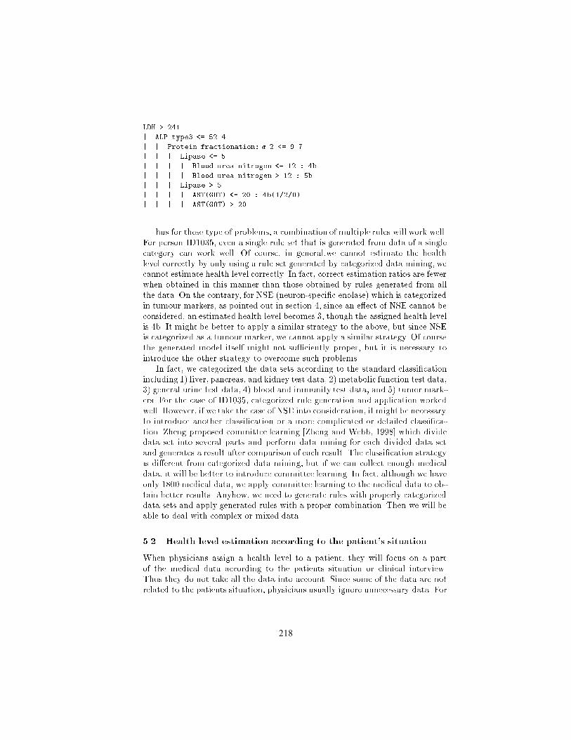
...LDH > 241| ALP type3 <= 52.4| | Protein fractionation:! 2 <= 9.7| | | Lipase <= 5| | | | Blood urea nitrogen <= 12 : 4b| | | | Blood urea nitrogen > 12 : 5b| | | Lipase > 5| | | | AST(GOT) <= 20 : 4b(1/2/0)| | | | AST(GOT) > 20.....hus for these type of problems, a combination of multiple rules will work well.For person ID1035, even a single rule set that is generated from data of a singlecategory can work well. Of course, in general,we cannot estimate the healthlevel correctly by only using a rule set generated by categorized data mining, wecannot estimate health level correctly. In fact, correct estimation ratios are fewerwhen obtained in this manner than those obtained by rules generated from allthe data. On the contrary, for NSE (neuron-speci�c enolase) which is categorizedin tumour markers, as pointed out in section 4, since an e�ect of NSE cannot beconsidered, an estimated health level becomes 3, though the assigned health levelis 4b. It might be better to apply a similar strategy to the above, but since NSEis categorized as a tumour marker, we cannot apply a similar strategy. Of coursethe generated model itself might not su�ciently proper, but it is necessary tointroduce the other strategy to overcome such problems.In fact, we categorized the data sets according to the standard classi�cationincluding 1) liver, pancreas, and kidney test data, 2) metabolic function test data,3) general urine test data, 4) blood and immunity test data, and 5) tumor mark-ers. For the case of ID1035, categorized rule generation and application workedwell. However, if we take the case of NSE into consideration, it might be necessaryto introduce another classi�cation or a more complicated or detailed classi�ca-tion. Zheng proposed committee learning [Zheng and Webb, 1998] which dividedata set into several parts and perform data mining for each divided data setand generates a result after comparison of each result. The classi�cation strategyis di�erent from categorized data mining, but if we can collect enough medicaldata, it will be better to introduce committee learning. In fact, although we haveonly 1800 medical data, we apply committee learning to the medical data to ob-tain better results. Anyhow, we need to generate rules with properly categorizeddata sets and apply generated rules with a proper combination. Then we will beable to deal with complex or mixed data.5.2 Health level estimation according to the patient's situationWhen physicians assign a health level to a patient, they will focus on a partof the medical data according to the patients situation or clinical interview.Thus they do not take all the data into account. Since some of the data are notrelated to the patients situation, physicians usually ignore unnecessary data. For218

a better estimation of health levels, it might be necessary to prepare or installsuch an intuitional reasoning as physicians do. That is, during the health levelestimation procedure, the system should focus on proper data clusters, and applyrules related to the data clusters.As shown above, we conducted categorized data mining and applied the gen-erated rule sets to determine health levels. Currently we have not discoveredgeneral models for generation and applying rules. However, as shown above, wediscovered several case that can estimate health levels correctly. Therefore, itis necessary to develop an automatic categorization method that can properlycategorize medical data. Simple Principal Component Analysis could not prop-erly categorize the medical data sets. In fact, if we know the patient's situation,we can focus on the data category relating to the patient's organ which is thesource of the health problem. In the future, we will construct a data catego-rization model and a rule set combination model by analyzing data sets andphysicians' health level determination models.Finally, we can also say that the combination of categorized learning andcommittee learning will generate better result in data mining.6 ConclusionsIn this paper, we discussed the treatment of complex medical data which arecollected in the International Research and Educational Institute for IntegratedMedical Science (IREIIMS) project. Our main aim is to determine relationshipsbetween health levels and medical data. By applying C4.5, we could obtained ac-ceptable results, but for even better results, we suggested and introduced severalstrategies including categorized data mining and combined rule application. Wehave not discovered general models for categorization and combination.However,we point out that a general model can be obtained by referring to physicians'determination patterns. We need to discover more strong relationships betweenmedical data and health status.For relationship or association, Agrawal proposed an association rule thatrepresents relationships between items in databases [Agrawal et al., 1993]. Theassociation rule is frequently used when analyzing POS data to discover tenden-cies of users' shopping patterns (basket analysis). However, from the analysis,we can only discover frequently co-occurring patterns. Also, relational data min-ing has recently been proposed [D�zroski and Lavra�c, 2001]. This paradigm alsodiscovers relationships between items in a (relational) database by using ILPtechniques. Their approaches are important for complex data mining. Howeverour major aim is not to discover relationships between each category but to de-termine an e�ective classi�cation for data mining of complex data. Nevertheless,their concept can be introduced to discover relationships.Finally, we emphasize that our approach is based on a concept of chancediscovery [Ohsawa and McBurney, 2003]. A rare relationship that cannot be ex-tracted by simple C4.5 application can play a signi�cant role in a proper health219

level determination. Accordingly, our main aim is to discover such rare and sig-ni�cant relationships that can be used for accurate health level determination.AcknowledgmentsThis research was supported in part by the Program for Promoting the Establish-ment of Strategic Research Centers, Special Coordination Funds for PromotingScience and Technology, Ministry of Education, Culture, Sports, Science andTechnology (Japan). We thank Mr. Ken Chang (NTT-AT) for supporting todevelop analysis tools.References[Abe et al., 2004] Abe A., Naya F., Kogure K., and Hagita N.: Rule Acquisition fromsmall and heterogeneous data set, Technical Report of JSAI, SIG-KBS-A304-32, pp.189{194 (2004) in Japanese[Abe et al., 2007a] Abe A, Hagita N, Furutani M, Furutani Y, and Matsuoka R.: Pos-sibility of Integrated Data Mining of Clinical Data, Data Science Journal, Vol. 6,Supplement, pp. S104{S115 (2007)[Abe et al., 2007b] Abe A, Hagita N, Furutani M, Furutani Y, and Matsuoka R.: Aninterface for medical diagnosis support, Proc. of KES2007 (2007) to appear[Agrawal et al., 1993] Agrawal R., Imielinski T., and Swami A.: Mining associationrules between sets of items in large databases, Proc. of ACM SIGMOD Int'l Conf.on Management of Data, pp. 207{216 (1993)[D�zroski and Lavra�c, 2001] D�zroski S and Lavra�c N eds.: Relational Data Mining,Springer Verlag (2001)[Ichise and Numao, 2003] Ichise R., Numao M.: A Graph-based Approach for Tem-poral Relationship Mining, Technical Report of JSAI, SIG-FAI-A301, pp. 121{126(2003)[Ichise and Numao, 2005] Ichise R. and Numao M.: First-Order Rule Mining by UsingGraphs Created from Temporal Medical Data, LNAI, Vol. 3430, pp. 112{125 (2005)[Kobayashi and Kawakubo, 1994] Kobayashi T. and Kawakubo T.: Prospective Inves-tigation of Tumor Markers and Risk Assessment in Early Cancer Screening, Cancer,Vol. 73, No. 7, pp. 1946{1953 (1994)[Ohsawa, 2003] Ohsawa Y., Okazaki N., and Matsumura N.: A Scenario Developmenton Hepatics B and C, Technical Report of JSAI, SIG-KBS-A301, pp. 177{182 (2003)[Ohsawa and McBurney, 2003] Osawa Y. and McBurney P. eds.: Chance Discovery,Springer Verlag (2003)[Tsumoto, 2004] Tsumoto S.: Mining Diagnostic Rules from Clinical Databases UsingRough Sets and Medical Diagnostic Model, Information Sciences, Vol. 162, No. 2,pp. 65{80 (2004)[Quinlan, 1993] Quinlan J.R.: C4.5: Programs for Machine Learning, Morgan Kauf-man (1993)[Zheng and Webb, 1998] Zheng Z. and Webb G.I.: Stochastic Attribute Selection Com-mittees, Proc. of AI98, pp. 321{332 (1998)220

POM Centric Multiaspect Data Analysis forInvestigating Human Problem Solving Function

Shinichi Motomura1, Akinori Hara1, Ning Zhong2,3, and Shengfu Lu3

1 Graduate School, Maebashi Institute of Technology, Japan2 Department of Life Science and Informatics, Maebashi Institute of Technology,

Japan3 The International WIC Institute, Beijing University of Technology, China

motomura@maebashi-it.org

Abstract. In the paper, we propose an approach of POM (peculiarityoriented mining) centric multiaspect data analysis for investigating hu-man problem solving related functions, in which computation tasks areused as an example. The proposed approach is based on Brain Infor-matics (BI) methodology, which supports studies of human informationprocessing mechanism systematically from both macro and micro pointsof view by combining experimental cognitive neuroscience with advancedinformation technology. We describe how to design systematically cogni-tive experiments to obtain multi-ERP data and analyze spatiotemporalpeculiarity of such data. Preliminary results show the usefulness of ourapproach.

1 Introduction

Problem-solving is one of main capabilities of human intelligence and has beenstudied in both cognitive science and AI [9], where it is addressed in conjunctionwith reasoning centric cognitive functions such as attention, control, memory,language, reasoning, learning, and so on. We need to better understand howhuman being does complex adaptive, distributed problem solving and reasoning,as well as how intelligence evolves for individuals and societies, over time andplace [3, 11–13, 17]. Then, we catch problem solving from the standpoint of BrainInformatics, and address systematically for the solution of a process.

Brain Informatics (BI) is a new interdisciplinary field to study human infor-mation processing mechanism systematically from both macro and micro pointsof view by cooperatively using experimental, theoretical, cognitive neuroscienceand advanced information technology [16, 17]. It attempts to understand humanintelligence in depth, towards a holistic view at a long-term, global vision tounderstand the principles, models and mechanisms of human information pro-cessing system.

Our purpose is to understand activities of human problem solving systemby investigating the spatiotemporal features and flow of human problem solv-ing system, based on functional relationships between activated areas of humanbrain. More specifically, at the current stage, we want to understand:

221

– how a peculiar part (one or more areas) of the brain operates in a specifictime;

– how the operated part changes along with time;– how the activated areas work cooperatively to implement a whole problem

solving system;– how the activated areas are linked, indexed, navigated functionally, and what

are individual differences in performance.

Based on this point of view, we propose a way of peculiarity oriented mining(POM) for knowledge discovery in multiple human brain data.

The rest of the paper is organized as follows. Section 2 provides a BI Method-ology for multiaspect human brain data analysis of human problem solving sys-tem. Sections 3 explain how to design the experiment of an ERP mental arith-metic task with visual stimuli standing on BI Methodology. Sections 4 describehow to do multiaspect analysis in the obtained ERP data, respectively, as anexample to investigate human problem solving and to show the usefulness of theproposed mining process. Finally, Section 5 gives concluding remarks.

2 Brain Informatics Methodology

Brain informatics pursues a holistic understanding of human intelligence througha systematic approach to brain research. BI regarded the human brain as aninformation processing system (HIPS) and emphasizes cognitive experiments tounderstand its mechanisms for analyzing and managing data. Such systematicstudy includes the following 4 main research issues:

– systematic investigation of human thinking centric mechanisms;– systematic design of cognitive experiments;– systematic human brain data management;– systematic human brain data analysis.

The first issue is based on the observation for Web intelligence researchneeds and the state-of-the-art cognitive neuroscience. In cognitive neuroscience,although many advanced results with respect to “perception oriented” studyhave been obtained, only a few of preliminary, separated studies with respectto “thinking oriented” and/or a more whole information process have been re-ported [1].

The second issue is with respect to how to design the psychological and phys-iological experiments for obtaining various data from HIPS, in a systematic way.In other words, by systematic design of cognitive experiments in BI methodol-ogy, the data obtained from a cognitive experiment and/or a set of cognitiveexperiments may be used for multi-task/purpose.

The third issue relates to manage human brain data, which is based on aconceptual model of cognitive functions that represents functional relationshipsamong multiple human brain data sources for systematic investigation and un-derstanding of human intelligence.

222

The last issue is concerned with how to extract significant features from mul-tiple brain data measured by using fMRI and EEG in preparation for multiaspectdata analysis by combining various data mining methods with reasoning [4, 6,10, 11, 15].

An investigation flow based on BI methodology is shown in Figure 1, in whichvarious tools can be cooperatively used in the multi-step process for experi-mental design, pre-processing (data extraction, modeling and transformation),multiaspect data mining and post-processing.

Data extraction Model transform

ERP dataDataMining

Explanation/Synthesis of mining results

Knowledge Discovery

Experiment

Integration ofResults

(Multi-AspectData Mining)

Spectrum data

DataMining

fMRI Image data

DataMining

Data Mining partExperimentalDesign part

Data collection

Perception: Auditory: Visual: Tactualetc.

Thinking(Task): Computation : Reasoning: Learningetc.

Memory,Attention, etc.

Data extraction Model transform

ERP dataDataMining

Explanation/Synthesis of mining results

Knowledge Discovery

Experiment

Integration ofResults

(Multi-AspectData Mining)

Spectrum data

DataMining

fMRI Image data

DataMining

Data Mining partExperimentalDesign part

Data collection

Perception: Auditory: Visual: Tactualetc.

Thinking(Task): Computation : Reasoning: Learningetc.

Memory,Attention, etc.

Fig. 1. A flow based on BI methodology

3 The Experiment of Mental Arithmetic Task withVisual Stimuli

As mentioned above, based on BI methodology, the data obtained from a cog-nitive experiment and/or a set of cognitive experiments may be used for multi-task/purpose, including for investigating both lower and higher functions ofHIPS. For example, it is possible that our experiment can meet the followingrequirements: investigating the mechanisms of human visual and auditory sys-tems, computation, problem-solving (i.e. the computation process is regarded asan example of problem-solving process), and the spatiotemporal feature and flowof HIPS in general. Figure 2 gives a computation process from the macro view-points, with respect to several component functions of human solving problem,such as attention, interpretation, short-term memory, understanding of work,computation, checking.

223

1. Attention of figure2. Interpretation of figure 3. Memory of figure4. Confirmation of work (+)5. Attention of figure6. Interpretation of figure 7. Memory of figure8. Addition 9. Memory of sum10. Comparison of sum

augend

addend+

sum=

1,5

1,52,6

3,4,7,8,9,101. Attention of figure2. Interpretation of figure 3. Memory of figure4. Confirmation of work (+)5. Attention of figure6. Interpretation of figure 7. Memory of figure8. Addition 9. Memory of sum10. Comparison of sum

augend

addend+

sum=

1,5

1,52,6

3,4,7,8,9,10

Fig. 2. Computation as an example of problem-solving

In this work, the ERP (event-related potential) human brain waves are de-rived by carrying out a mental arithmetic task with visual stimuli, as an exam-ple to investigate human problem solving process. ERP is a light, sound, andbrain potential produced with respect to the specific phenomenon of spontaneousmovement [2].

3.1 Outline of Experiments

The experiment conducted this time shows a numerical calculation problem toa subject, and asks the subject to solve it in mental arithmetic, and the shownsum has hit, or it pushes a button, and performs a judging of corrigenda. Theform of the numerical calculation to be shown is the addition problem of “au-gend + addend = sum”. The wrong sum occurs at half the probability, and thedistribution is not uniform.

In the experiments, three states (tasks), namely, visual on-task, visual off-task, and no-task, exist by the difference in the stimulus given to a human subject.Visual on-task is the state which is calculating by looking a number. Visual off-task is the state which is looking the number that appears at random. no-task isthe relaxed state which does not work at all.

Figure 3 gives an example of the screen state transition. Type 1 is two digitsaddition that the figure remains on the screen. Type 2 is also two digits addition,but the figure doesn’t remain on the screen.

We try to compare and analyze what is the relationship between tasks. Fig-ure 4 gives an example of comparing tasks. By this design, it is possible toanalyze the influence, in the different levels of difficulty, with the same on-taskand off-task, and to make a comparison between on-task and off-task in the samedifficulty.

3.2 Trigger Signal and Timing Chart

It is necessary to measure EEG relevant to a certain event to the regular timingin measurement of ERP repeatedly. In this research, since the attention was paid

224

9

3 37+24=37+2437+237+37 37+24=61

96271962796296 962715489627154962715

3 +7

9 26 7

42

1

61=

845

Type 1 On-task (ex. 37+24=61)

Type 2 On-task (ex. 37+24=61)

・・・

・・・

Type 1 Off-task (ex. 9,6,2,7,1,5,4,8,…)

Type 2 Off-task (ex. 9,6,2,7,1,5,4,8,…)

9

3 37+24=37+2437+237+37 37+24=61

96271962796296 962715489627154962715

3 +7

9 26 7

42

1

61=

845

Type 1 On-task (ex. 37+24=61)

Type 2 On-task (ex. 37+24=61)

・・・

・・・

Type 1 Off-task (ex. 9,6,2,7,1,5,4,8,…)

Type 2 Off-task (ex. 9,6,2,7,1,5,4,8,…)

Fig. 3. Experimental design with two levels of difficulty

3 37+24・・・・・・・・・・・・37+237+37

9 96271・・・・・・・・・・・・962796296

4 +7 9・・・・・・・・・・・・1

8 45 3 7・・・・・・・・・・・・

Type 1　On-task

Type 2　On-task

Compare On-tasks(difference of showing)

Type 1　Off-task

Type 2　Off-task Compare On and Off-tasks Compare On and Off-tasks

Compare Off-tasks(difference of showing)

3 37+24・・・・・・・・・・・・37+237+373 37+24・・・・・・・・・・・・37+237+37

9 96271・・・・・・・・・・・・9627962969 96271・・・・・・・・・・・・962796296

4 +7 9・・・・・・・・・・・・14 +7 9・・・・・・・・・・・・1

8 45 3 7・・・・・・・・・・・・8 45 3 7・・・・・・・・・・・・

Type 1　On-task

Type 2　On-task

Compare On-tasks(difference of showing)

Type 1　Off-task

Type 2　Off-task Compare On and Off-tasks Compare On and Off-tasks

Compare Off-tasks(difference of showing)

Fig. 4. Viewpoints for experiments

225

to each event of augend, addend, and sum presentation in calculation activities.Pre-trigger was set to 200 [msec], and addition between two digits are recordedin 10000 [msec], respectively. Figure 5 gives an example of the time chart. “au” isaugend, “ad” is addend, and “su” is sum. Therefore “au2” is MSD (last 2-digits)of augend, and “au1” is LSD (last 1-digits) of augend. “n” is the random number(1-digits).

au2 au1 + ad2 ad1 = Rest time

1000 6000

10200 (Pre-trigger = 200msec)

Trigger Signal: Recording Time

Time[msec]

Sum

1000 2000 1000 1000 2000 2000

au2・・・

au2 au1 + ad2 ad1 = Rest time

1000 6000

10200 (Pre-trigger = 200msec)

Trigger Signal: Recording Time

Time[msec]

Sum

1000 2000 1000 1000 2000 2000

au2・・・

(a) Timing chart of on-task

n1 n2 n3 n4 n5

1000 Time[msec]

Rest timen7n6 n8

10200 (Pre-trigger = 200msec)Trigger Signal

n9 n10・・・

: Recording Time

60001000 1000100010001000 1000100010001000

n1 n2 n3 n4 n5

1000 Time[msec]

Rest timen7n6 n8

10200 (Pre-trigger = 200msec)Trigger Signal

n9 n10・・・

: Recording Time

60001000 1000100010001000 1000100010001000

(b) Timing chart of off-task

Fig. 5. Timing chart

3.3 Experimental Device and Measurement Conditions

Electroencephalographic activity was recorded using a 64 channel BrainAmpamplifier (Brain Products, Munich, Germany) with a 64 electrode cap. The elec-trode cap is based on an extended international 10-20 system. Furthermore, eyemovement measurement (2ch) is also used. The sampling frequency is 2500Hzto be processed. The number of experimental subjects is 20.

4 Multiaspect Data Analysis (MDA)

4.1 Topography Analysis

For the measured EEG data, a maximum of 40 addition average processingwere performed, and the ERPs were derived by using Brain Vision Analyzer(Brain Products, Munich, Germany). Generally speaking, the Wernicke areaof a left temporal lobe and the prefrontal area are related to the calculation

226

process [5]. In this study, we pay attention to recognition of the number, short-term memory and attentiveness, as well as compare Type 1 and Type 2 byfocusing on important channels (C5).

Figure 6 shows the topography. After displayed symbol, the display time is250 milliseconds. We can see some difference between Type 1 and Type 2 atthe appearance part (the left and right brain) of the positive potential. Thisphenomenon means the process of recognition of number and expression aredifferent between Type 1 and Type 2.

au2 au1 + ad2 ad1 = sum

Type 1On-task

Type 1Off-task

Type 2On-task

Type 2Off-task

[uV]

C5

au2 au1 + ad2 ad1 = sum

Type 1On-task

Type 1Off-task

Type 2On-task

Type 2Off-task

[uV]

Type 1On-task

Type 1Off-task

Type 2On-task

Type 2Off-task

[uV]

C5

Fig. 6. Topography of ERP data

First, we discuss the on-task and off-task. We can see some difference betweenon-task and off-task at the positive potential. It is guessed that on-task is linkedto the activating of frontal area. Next, we discuss the frontal area. We can seesome difference between Type 1 and Type 2 at the distribution of the positivepotential. Type 1 shows high positive potential in almost time. It is guessed thatType 1 is easier than Type 2 to recognize the number, then the experimentalsubject repeated computation in Type 1. Finally, we discuss the channel C5,which is part of the left temporal lobe with respect to the logical interpretation.Generally speaking, when human interprets and calculates the expression, theleft brain is activated. In particular, the area with respect to short-term memoryis strongly activated for Type 2. In addition, the experimental subject logicallyinterprets an each figure. Therefore, it is guessed that the potential distributionof Type 2 is different from the one of Type 1 in C5. It is necessary to investigate

227

this phenomenon deeply additionally with the change of the time series aroundthe visual area.

4.2 Peculiarity Oriented Mining

It is clear that a specific part of the brain operates in a specific time and theoperations change over time. Although detecting the concavity and convexity(P300 etc.) of ERP data is easy by using the existing tool, it is difficult to find apeculiar one in multiple channels with the concavity and convexity [7, 8]. In orderto discover new knowledge and models of human information processing activi-ties, it is necessary to pay attention to the peculiar channel and time in ERPsfor investigating the spatiotemporal features and flow of a human informationprocessing system.

peculiarity oriented mining (POM) is a proposed knowledge discovery method-ology [14, 15]. The main task of POM is the identification of peculiar data. Theattribute-oriented method of POM, which analyze data from a new view andare different from traditional statistical methods, has been recently proposedby Zhong et al. and applied in various real-world problems [14, 15]. Unfortu-nately, such POM is not totally fit for ERP data analysis. The reason is thatthe useful aspect for ERP data analysis is not amplitude, but the latent time.In order to solve this problem, we extend POM to Peculiarity Vector OrientedMining (PVOM). After smoothing enough by moving average processing, in thetime series, we pay the attention to each potential towards N pole or P pole.Furthermore, the channel with the direction different from a lot of channels isconsidered to be a peculiar channel at that time. Hence, the distance betweenthe attribute-values is expressed at the angle. And this angle can be obtainedfrom the inner product and the norm in the vector. Let inclination of wave i ina certain time t be xit. The extended PF (Peculiarity Factor) corresponding toERP can be defined by the following Eq. (1).

PF (xit) =n∑

k=1

θ(xit, xkt)α. (1)

α = 0.5 as default. In normally POM, PF is obtained by distance between twoattribute values. However, θ in Eq. (1) is an angle which the wave in time tmakes. For the θ, we can compute for an angle using Eq. (2).

cosθ =1 + xit · xkt√

1 + x2it

√1 + x2

kt

. (2)

Based on the peculiarity factor, the selection of peculiar data is simply carriedout by using a threshold value. More specifically, an attribute value is peculiarif its peculiarity factor is above minimum peculiarity p, namely, PF (xit) ≥ p.The threshold value p may be computed by the distribution of PF as follows:

threshold = mean of PF (xit) + (3)β × standard deviation of PF (xit)

228

where β can be adjusted by a user, and β = 1 is used as default. The thresholdindicates that a data is a peculiar one if its PF value is much larger than themean of the PF set. In other words, if PF (xit) is over the threshold value, xit

is a peculiar data. By adjusting the parameter β, a user can control and adjustthe threshold value.

4.3 Application of the Extended POM Method

In this work, we want to mine four kinds of patterns, which are classified intotwo types of peculiarity with respect to the temporal and channel axises, respec-tively, as shown in Figure 7. Mining 1 and Mining 2 are used to find temporalpeculiarity, and Mining 3 and Mining 4 are used to find channel peculiarity,respectively.

.

.

　　　　　　　　　　　　　　　　　　　　　　　　　　　　.　　　　　　　　

.

.

.

.

.

.

.

.

.

.

.

.

.

.

.

.

.

.

……CH3

……CH2

……CH1

…t=2t=1t=0…t=-500

Channel-PeculiarityTrigger

Baseline Potential Event Related Potential (ERP)Temporal-Peculiarity

Mining 1 (POM)

Mining 2 (POM)Mining 3 (POM)Mining 4 (PVOM)

Event: Pre-Trigger

.

.

　　　　　　　　　　　　　　　　　　　　　　　　　　　　.　　　　　　　　

.

.

.

.

.

.

.

.

.

.

.

.

.

.

.

.

.

.

……CH3

……CH2

……CH1

…t=2t=1t=0…t=-500

Channel-PeculiarityTrigger

Baseline Potential Event Related Potential (ERP)Temporal-Peculiarity

Mining 1 (POM)

Mining 2 (POM)Mining 3 (POM)Mining 4 (PVOM)

Event: Pre-Trigger

Fig. 7. Views of ERP peculiarity

More specifically, Mining 1 examines whether the potential at arbitrary timeis peculiar compared with a baseline potential in channel C5. Mining 2 examineswhether the potential at arbitrary time is peculiar compared with an ERP inchannel C5. Mining 3 examines whether the potential of C5 is peculiar comparedwith the potential on other channels in a specific time. Furthermore, Mining 4examines whether a potential change of C5 is peculiar compared with a potentialchange on other channels in a specific time. As shown in Figure 7, the POMmethod is used for the Mining 1 to Mining 3 and the extended POM method(PVOM) stated in Section 4.2 is used for the Mining 4. PF axis 0 in Figs. 8 and9 denotes the threshold and the part is peculiar if it is over the threshold value.

Figure 8 shows an ERP and the result of mining on it, in which the peculiarityin ERP data with respect to addition Type 1 (Channel: C5, Task: off-task)is presented. We can see there are some higher values of peculiarity and thepotential changes over the time. Although the off-task potential is about zero,Viewpoint 1 is nevertheless judged to be peculiar because it is a higher positive

229

at this time. Furthermore, Viewpoint 2 represents that the potential of C5 ispeculiar at this time in the channel. Viewpoint 3 represents that a potentialchange of C5 is peculiar at this time in the channel.

-10

-5

0

5

10

-10

-5

0

5

10

-120

-60

0

60

120

ERP (Type: 1 Ch: C5)

Temporal axis POM (Off-task): On-task: Off-task

: Mining 3: Mining 4

: Mining 1: Mining 2

[uV]

PF value

Channel axis POM (Off-task)

au2:Event

+au1 ad2 ad1 = sumn1 n3n2 n5n4 n6 n7 n9n8 n10

Viewpoint 3

[msec]0 1000 30002000 4000 5000 6000 7000 8000 9000Task start

Viewpoint 2

PF valueViewpoint 1

-10

-5

0

5

10

-10

-5

0

5

10

-120

-60

0

60

120

ERP (Type: 1 Ch: C5)

Temporal axis POM (Off-task): On-task: Off-task: On-task: Off-task

: Mining 3: Mining 4: Mining 3: Mining 4

: Mining 1: Mining 2: Mining 1: Mining 2

[uV]

PF value

Channel axis POM (Off-task)

au2:Event

+au1 ad2 ad1 = sumn1 n3n2 n5n4 n6 n7 n9n8 n10

Viewpoint 3

[msec]0 1000 30002000 4000 5000 6000 7000 8000 9000Task start

Viewpoint 2

PF valueViewpoint 1

Fig. 8. ERP and mining results (Type 1 off-task)

Figure 9 shows an ERP and the result of mining on it, in which the peculiarityin ERP data with respect to addition Type 2 (Channel: C5, Task: on-task) ispresented. Although the on-task pencil is a higher positive one, Viewpoint 4 isjudged to be peculiar because it is near to zero. Furthermore, although otheron-task potentials are high, Viewpoint 5 is judged to be peculiar because it isremarkably high in comparison with others.

Figure 10 illustrates how to integrate the mining results, not only POM forERP data, but also frequency data and fMRI data. The system collects multipledata sources from several event-related time points, and transformed into variousforms for POM centric MDA. Furthermore, the results of separate analysis canbe explained and combined into a whole flow of information processing withrespect to problem solving.

5 Conclusion

In this paper, we investigated human problem solving related functions by usingcomputation as an example, which demonstrate what is BI methodology and

230

-150

-50

50

150

-8

-4

0

4

8

-200 1800 3800 5800 7800 9800

-6

0

6

12

au2:Event

+au1 ad2 ad1 = sumn1 n3n2 n5n4 n6 n7 n9n8 n10

Temporal axis POM (On-task)

Channel axis POM (On-task)

ERP (Type: 2 Ch: C5)[msec]0 1000 30002000 4000 5000 6000 7000 8000 9000

Viewpoint 5Viewpoint 4

[uV]

PF value

PF value

: On-task: Off-task

: Mining 1: Mining 2

: Mining 3: Mining 4

-150

-50

50

150

-8

-4

0

4

8

-200 1800 3800 5800 7800 9800

-6

0

6

12

au2:Event

+au1 ad2 ad1 = sumn1 n3n2 n5n4 n6 n7 n9n8 n10

Temporal axis POM (On-task)

Channel axis POM (On-task)

ERP (Type: 2 Ch: C5)[msec]0 1000 30002000 4000 5000 6000 7000 8000 9000

Viewpoint 5Viewpoint 4

[uV]

PF value

PF value

: On-task: Off-task: On-task: Off-task

: Mining 1: Mining 2: Mining 1: Mining 2

: Mining 3: Mining 4: Mining 3: Mining 4

Fig. 9. ERP and mining results (Type 2 on-task)

ERP dataC5

transformationtransformation transformationtransformationtransformationtransformation

POM/MDA POM/MDA POM/MDA POM/MDA

Explanation/Synthesis

other channels spectrumfrequency data fMRI data

imageERP data

C5transformationtransformation transformationtransformationtransformationtransformation

POM/MDA POM/MDA POM/MDA POM/MDA

Explanation/Synthesis

other channels spectrumfrequency data fMRI data

image

Fig. 10. Integration of mining results

231

its usefulness. The proposed POM centric multiaspect ERP data analysis basedon BI methodology shifts the focus of cognitive science from a single type ofexperimental data analysis towards a deep, holistic understanding of humaninformation processing principles, models and mechanisms.

Our future work includes obtaining and analyzing more subject data, com-bining with fMRI human brain image data for multi-aspect analysis in variousapproaches of data mining and reasoning.

References

1. M.S. Gazzaniga (ed.) The Cognitive Neurosciences III, The MIT Press (2004).2. T.C. Handy, Event-Related Potentials, A Methods Handbook, The MIT Press

(2004).3. J. Liu, X. Jin, and K.C. Tsui, Autonomy Oriented Computing: From Problem

Solving to Complex Systems Modeling, Springer (2005).4. V. Megalooikonomou and E.H. Herskovits, “Mining Structure-Function Associ-

ations in a Brain Image Database”, K.J. Cios (ed.) Medical Data Mining andKnowledge Discovery, Physica-Verlag (2001) 153-179.

5. H. Mizuhara, L. Wang, K. Kobayashi, Y. Yamaguchi, “Long-range EEG Phase-synchronization During an Arithmetic Task Indexes a Coherent Cortical NetworkSimultaneously Measured by fMRI”, NeuroImage, Vol.27, No.3 (2005) 553-563.

6. T.M. Mitchell, R. Hutchinson, R.S. Niculescu, F.Pereira, X. Wang, M. Just, andS. Newman, “Learning to Decode Cognitive States from Brain Images”, MachineLearning, 57(1-2) (2004) 145-175.

7. H. Nittono, Y. Nageishi, Y. Nakajima, and P. Ullsperger, “Event-related PotentialCorrelates of Individual Differences in Working Memory Capacity”, Psychophysi-ology, 36 (1999) 745-754.

8. T.W. Picton, S. Bentin, P. Berg, E. Donchin, S.A. Hillyard, R. Johnson, et al.“Guidelines for using human event-related potentials to study cognition: Recordingstandards and publication criteria”, Psychophysiology, 37, (2000) 127-152.

9. A. Newell and H.A. Simon, Human Problem Solving, Prentice-Hall (1972).10. F.T. Sommer and A. Wichert (eds.) Exploratory Analysis and Data Modeling in

Functional Neuroimaging, The MIT Press (2003).11. R.J. Sternberg, J. Lautrey, and T.I. Lubart, Models of Intelligence, American Psy-

chological Association (2003).12. Y.Y. Yao, “A Partition Model of Granular Computing”, Springer LNCS Transac-

tions on Rough Sets, 1 (2004) 232-253.13. L.A. Zadeh, “Precisiated Natural Language (PNL)”, AI Magazine, 25(3) (Fall

2004) 74-91.14. N. Zhong, Y.Y. Yao, and M. Ohshima, “Peculiarity Oriented Multi-Database Min-

ing”, IEEE Transaction on Knowledge and Data Engineering, 15(4) (2003) 952-960.15. N. Zhong, J.L. Wu, A. Nakamaru, M. Ohshima, H. Mizuhara, “Peculiarity Oriented

fMRI Brain Data Analysis for Studying Human Multi-Perception Mechanism”,Cognitive Systems Research, 5(3), Elsevier (2004) 241-256.

16. N. Zhong, “Building a Brain-Informatics Portal on the Wisdom Web with a Multi-Layer Grid: A New Challenge for Web Intelligence Research”, V. Torra et al. (eds.)Modeling Decisions for Artificial Intelligence, LNAI 3558, Springer (2005) 24-35.

17. N. Zhong, “Impending Brain Informatics (BI) Research from Web Intelligence(WI) Perspective”, International Journal of Information Technology and DecisionMaking, World Scientific, Vol. 5, No. 4 (2006) 713-727.

232

Author Index

Abe, Akinori, 209Abe, Hidenao, 49

Bahri, Emna, 151Basile, T.M.A., 13Bathoorn, Ronnie, 25Biba, M., 13

Ceci, Michelangelo, 83Ciesielski, Krzysztof, 128

d’Amato, Claudia, 197Delteil, Alexandre, 106Dembczynski, Krzysztof, 163Di Mauro, N., 13

El Sayed, Ahmad, 185Elazmeh, William, 37Esposito, Floriana, 13, 197

Fanizzi, Nicola, 197Farion, Ken, 37Ferilli, S., 13Furutani, Michiko, 209Furutani, Yoshiyuki, 209

Grcar, Miha, 1Grobelnik, Marko, 1

Hacid, Hakim, 185Hagita, Norihiro, 209Hara, Akinori, 221Hirabayashi, Satoru, 49Hirano, Shoji, 139

Kolczynska, Elzbieta, 175Kontkiewicz, Aleksandra, 106Kotłowski, Wojciech, 163Kryszkiewicz, Marzena, 106Kłopotek, Mieczysław A., 128

Lu, Shengfu, 221

Maddouri, Mondher, 151Malerba, Donato, 83Marcinkowska, Katarzyna, 106Matsuoka, Rumiko, 209Matwin, Stan, 37Michalowski, Wojtek, 37Mladenic, Dunja, 1Motomura, Shinichi, 221

Nicoloyannis, Nicolas, 151

O’Sullivan, Dympna, 37Ohsaki, Miho, 49Okawa, Takenao, 71Ozaki, Tomonobu, 71

Peters, James F., 116Protaziuk, Grzegorz, 106

Ras, Zbigniew W., 59, 95Ramanna, Sheela, 116Rybinski, Henryk, 106

Sehatkar, Morvarid, 37Siebes, Arno, 25Słowinski, Roman, 163

Tsumoto, Shusaku, 139

Wieczorkowska, Alicja, 175Wierzchon, Sławomir, 128Wilk, Szymon, 37Wyrzykowska, Elzbieta, 95

Yamaguchi, Takahira, 49Yamamoto, Tsubasa, 71

Zhang, Xin, 59Zhong, Ning, 221Zighed, Djamel, 185

233