me 581: simulation of mechanical systems inverse ... · mechanism. link 1 – solar panel frame...

ME 581: Simulation of Mechanical

Systems Inverse Kinematics of a 3-Degree of

Freedom Solar Tracker

Greg Brulo

Abstract

ARPA-E’s MOSAIC (Micro-scale Optimized Solar-cell Arrays

with Integrated Concentration) program’s goal is to “lower the

cost of solar systems by using integrated concentration to

significantly increase PV module efficiency without increasing

manufacturing costs.” The Pennsylvania State University’s

solution to this problem requires actuators to move the PV

(photovoltaic) cells throughout the day to keep them in the path

of the concentrated light. This report covers the kinematic

analysis of a concept actuation system. The goal of the analysis

is to determine if the current actuator concept is feasible.

2. Methodology

2.1. 2D Model Development and Definitions

The notation used in the kinematic analysis was the

E. J. Haug method. [1]

{ri} - the global position of the origin of the

reference frame attached to body i

{ri}P – global position of point P attached to body i

{si}’P - position of point P on body i relative to the

reference frame for body i measured in local body-

fixed directions.

{dij} – relative location between two points on

bodies i and j measured in global directions

[Ai] – orthonormal rotation matrix that describes

attitude of body i

[2]

Figure 1 illustrates the link locations on the

mechanism.

Link 1 – Solar panel frame

Link 3 – Middle sheet containing photovoltaic cells

Links 2,4,5 – Actuation wires (variable length)

Links 6,7,8 – Springs (variable length)

The links connect from points on the frame (link 1)

to points on the middle sheet (link 3). For example

link 2 connects point A on the frame to point A on

the middle sheet. The diagram shows point A and

point J to be at the same location on the middle

sheet. This is only true in this configuration.

Different design iterations may position points A

and J at a place along the edge other than at the

corner. The location of these points are controlled

in the MATLAB code found in Appendix 2.

The 2D model representation allows the middle

sheet to move in a planar method. It is allowed to

translate in two directions and rotate on the frame.

When the middle sheet is centered the local origin

for link 3 is coincident with the global origin on link

1 as seen in Figure 1.

2.2. Inverse Kinematics

The goal of the analysis is to determine if the

current actuator concept is feasible. An inverse

kinematics analysis was chosen since to determine

the lengths and forces for each link for a given

location of the middle sheet (link 3). A feasible

concept requires the control wires (links 2,4,5) to

maintain tension for all positions of the middle

sheet.

Global locations for each point were solved using

the transformation equation (1.1).

Figure 1: Mechanism diagram

(1.1)

{ri}P={ri}+[Ai]{si}’P [2]

Vectors {dij} describe the length and orientation of

each links.

(1.2)

{dij} = {rj}P-{ri}P [2]

The link length and angle were derived from

equation (1.2).

Spring forces were solved once the length and

angles of links 6, 7 and 8 were known.

(1.3)

Fi=(Li-Li_initial)*ki+initial_tensioni

where:

Li – initial length of link i

Li_initial – initial length (length when r3 = {0,0}T)

ki – spring rate for link i

initial_tensioni- tension when Li=Li_initial

Three equations were used to solve for the forces

from links 2, 4 and 5. These three equations were

the sum of forces in the global x direction on link 3,

sum of forces in the global y direction on link 3 and

the sum of moments about the local origin on link

3. The local origin of link 3 was at the center of

gravity location. These equations can be found in

the MATLAB code. The forces from links 2, 4, 5,

6, 7 and 8 can be found in Figure 2.

Figure 2: Forces on link 3

2.3. Inverse Kinematics and MATLAB

Execution

After the equations for finding the link lengths,

angles, locations and forces were derived, they

were executed in MATLAB. The MATLAB code

loads two files near the beginning which load the

configurable blue print geometry for links 1 and 3.

Spring parameters for links 6, 7 and 8 can be

configured in the main code for design iterations.

The path for link 3 must be chosen by the operator.

The operator can load a predetermined path or

manual place link 3 in the positions the operator is

interested in.

Once all the parameters are loaded, the MATLAB

code uses a for loop to solve the kinematics at each

position of link 3 in the path. The code uses the

MATLAB linear system of equations solver to

solve the 3 equations for the forces from links 2, 4

and 5 inside the for loop.

Once the for loop solves the kinematics at each

position of the path, the MATLAB code loads the

next path if required. This allows the user to

execute the kinematic solution for multiple paths.

3. Simulation and Results

The feasibility of the design was evaluated by

positioning the link 3 in different positions about its

maximum envelope of travel. The middle sheet

must be actuated +/- 10 mm in both the global x and

global y direction from a centered position. Link 3

is considered centered when the global position of

its origin is {0,0}T.

After either link 1 or link 3 geometry changed, the

initial lengths of links 6, 7 and 8 needed

calculated. This was done by loading a manual

path for link 3 into the MATLAB simulation. The

manual path placed link 3 in its centered position.

These initial lengths were then included in the

parameters for the springs.

The first design concept tested did not include

links 7 and 8. This design only used one spring,

link 6. Unfortunately this design was not feasible

since link 2 was in compression when the global

location of link 3 was {10,0}T.

After the first design concept did not work springs

7 and 8 were added. This concept worked at most

positions of link 3. Some positions of link 3

required either link 2, 4 or 5 to be in compression.

This compression could be corrected at the given

position by changing the spring attachment points

on link 1. However this practice resulted in a link

having a compressive force at a different location

of link 3.

A hypothesis was made describing the

phenomenon of not being able to have a single set

of spring geometry which results in tension of

links 2, 4 and 5 at every position of link 3 was

caused by the dramatic angle changes of the

springs. The change in transmission angle of link 8

can be seen in Figure 3. The transmission angle

changes from 63° to 90° to 153° in the given

example. The hypothesis describes the reason for

the links changing from tension to compression is

a direct result of the larger than ideal transmission

angle changes of the spring links such as link 8.

Figure 3: Link 8 transmission angle changes

If the length of links 2, 4, 5, 6, 7 and 8 were made

significantly longer than the movement of link 3

then the change in the transmission angles would

be small. This was tested by moving the perimeter

of link 1 away from the perimeter of link 3 by 410

mm. The original perimeter of link 1 was 180 x

180 mm. The new perimeter of link 1 was now

1000 x 1000 mm.

The blue print information for link 1 was updated

in MATLAB and the analysis was repeated. Now

links 2, 4 and 5 maintain tension at every position

of link 3.

A sample path for how the solar tracker would

move link 3 throughout the day was loaded into

the MATLAB model. This path represents an

implementation of the solar tracker in State

College Pennsylvania. Appendix 1 shares the

position data and force data for this application.

4. Conclusion

This model was successfully used to

evaluate the feasibility of the PSU MOSAIC

design concept. The model showed the first

concept was not feasible. A second concept

was created based on these results. The second

concept was proven to be feasible based on an

analysis using this model. This tool will be used

to study further iterations of the design

concepts after publishing this report.

References

[1] Haug, Edward J. Computer Aided

Kinematics and Dynamics of Mechanical

Systems. Boston: Allyn and Bacon, 2010.

Print.

[2] Sommer, H. J., III. "ME 581 Simulation of

Mechanical Systems - Spring 2017." ME

581, H.J. Sommer III. N.p., n.d. Web. 03

May 2017.

Appendix 1

The kinematic and force results simulate the latest design concept in State College Pennsylvania. This

design uses the small transmission angle shifts therefore the spring and control wires are longer than

ideal.

Appendix 2

The MATLAB code for the inverse kinematics model is shared here. Some of the code originates from

Dr. Sommer’s website as cited for reference [2].

% File name - MOSAIC_kinematic_forces_main_rev_4.m % - rev 4 - added spring in top left corner

% Greg Brulo % MOSAIC Kinematics % Spring 2017

% Use vector and matrix notation from Dr. Sommers Notes 04 01.

% ideas % 1 - have interrupt to confirm the parameters are all set

% Units are in mm, sec, N, radians

clear clear all clc

d2r=pi/180; % convert from degrees to radians

% Load the blue print information for link 1 and link 3 MOSAIC_Link_1_Info_rev_1 MOSAIC_Link_3_Info_rev_1

% Load the path from Alex Grede

SC_equisol_20deg=load('SC_equisol_20deg.txt'); run_1_seq=SC_equisol_20deg(1:55,1); % integer run_1_x=SC_equisol_20deg(1:55,2); % mm run_1_y=SC_equisol_20deg(1:55,3); % mm

% run 1 data columns % 1 - seq number % 2 - X position mm % 3 - Y position mm

% Spring info % initial_length=60; % mm k6=0.04; % N/mm k7=0.04; % N/mm k8=0.04; % N/mm initial_tension_6=9; % Newtons initial_tension_7=9; % Newtons initial_tension_8=9; % Newtons %L6i=15; %%%% Update me %L7i=15; %%%% Update me %L8i=15; %%%% Update me L6i=601; %%%% Update me L7i=601; %%%% Update me L8i=425; %%%% Update me

% configure the tilt info mass=0; phi_incline=45; g=9.81;

% Path Info % make a path with the middle sheet centered in y direction %r3_path_1=zeros(201,2); %r3_path_1(:,1)=[-10:0.1:10];

% Load a path from a text file r3_path_1=[run_1_x,run_1_y]*2.2;

% make a path with the middle sheet at +10 y r3_path_2=ones(201,2)*10; r3_path_2(:,1)=[-10:0.1:10];

% make a path with the middle sheet at -10 y r3_path_3=ones(201,2)*-10; r3_path_3(:,1)=[-10:0.1:10];

% make a path based on actual data r3_path_4(:,1:2)=[run_1_x*2.25,run_1_y*2.25];

% make a test path r3_path_5=[10 -10;10 -10];

adb=1; while adb<=1 % create a while loop to solve each path clear r3_path info; % clear these variables if 1==adb % select the correct path r3_path=r3_path_1; elseif 2==adb r3_path=r3_path_2; elseif 3==adb r3_path=r3_path_3; elseif 4==adb r3_path=r3_path_4; elseif 5==adb r3_path=r3_path_5; else 'error assigning adb and picking r3_path' end

adn=1; adn_size=size(r3_path); adn_max=adn_size(1,1);

while adn<=adn_max

% Describe where the link 3 is relative to link 1 r3=r3_path(adn,:)'; % Location of r3 relative to r1 phi3=0*d2r; % Enter degrees, but store radians A3=[cos(phi3) -sin(phi3); sin(phi3) cos(phi3)]; % rotation matrix q3=[r3; phi3]; % generalized coordinates for link 3

r1=[0,0]'; % location of global origin (should be 0,0) phi1=0*d2r; % Angle of ground (should be 0) A1=[cos(phi1) -sin(phi1); sin(phi1) cos(phi1)]; % rotation matrix q1=[r1; phi1]; % generalized coordinates for link 1 (should be 0,0,0)

% global locations - Eq 2.4.8, page 33 (Dr. Sommer)

r1A = r1 + A1*s1pA; r1B = r1 + A1*s1pB; r1C = r1 + A1*s1pC; r1D = r1 + A1*s1pD; r1E = r1 + A1*s1pE; r1F = r1 + A1*s1pF; r1G = r1 + A1*s1pG; r1H = r1 + A1*s1pH; r1I = r1 + A1*s1pI; r1J = r1 + A1*s1pJ;

r3A = r3 + A3*s3pA; r3B = r3 + A3*s3pB; r3C = r3 + A3*s3pC; r3D = r3 + A3*s3pD; r3E = r3 + A3*s3pE; r3F = r3 + A3*s3pF; r3G = r3 + A3*s3pG; r3H = r3 + A3*s3pH; r3I = r3 + A3*s3pI; r3J = r3 + A3*s3pJ;

% find the link vectors

% length of wires and direction relative to the frame D2=r3A-r1A; D4=r3C-r1C; D5=r3B-r1B; D6=r3D-r1D; D7=r3I-r1I; D8=r3J-r1J;

% length of the wires from frame to link 3 L2=sqrt(D2(1,1)^2+D2(2,1)^2); L4=sqrt(D4(1,1)^2+D4(2,1)^2); L5=sqrt(D5(1,1)^2+D5(2,1)^2); L6=sqrt(D6(1,1)^2+D6(2,1)^2); L7=sqrt(D7(1,1)^2+D7(2,1)^2); L8=sqrt(D8(1,1)^2+D8(2,1)^2);

% angle of the wires relative to the frame phi2=abs(atan(D2(2,1)/D2(1,1))); phi4=abs(atan(D4(2,1)/D4(1,1))); phi5=abs(atan(D5(2,1)/D5(1,1))); phi6=abs(atan(D6(2,1)/D6(1,1))); phi7=abs(atan(D7(2,1)/D7(1,1))); phi8=abs(atan(D8(2,1)/D8(1,1)));

if(D2(1,1)>=0 && D2(2,1)>=0)

% quadrant 1 %'quadrant1' phi2=phi2; elseif(D2(1,1)<0 && D2(2,1)>=0) % quadrant 2 %'quadrant2' phi2=pi-phi2; elseif(D2(1,1)<0 && D2(2,1)<0) % quadrant 3 %'quadrant3' phi2=pi+phi2; elseif(D2(1,1)>=0 && D2(2,1)<0) % quadrant 4 %'quadrant4' phi2=2*pi-phi2; else % error 'error1'

end

if(D4(1,1)>=0 && D4(2,1)>=0) % quadrant 1 %'quadrant1' phi4=phi4; elseif(D4(1,1)<0 && D4(2,1)>=0) % quadrant 2 %'quadrant2' phi4=pi-phi4; elseif(D4(1,1)<0 && D4(2,1)<0) % quadrant 3 %'quadrant3' phi4=pi+phi4; elseif(D4(1,1)>=0 && D4(2,1)<0) % quadrant 4 %'quadrant4' phi4=2*pi-phi4; else %% error 'error2' end

if(D5(1,1)>=0 && D5(2,1)>=0) % quadrant 1 %'quadrant1' phi5=phi5; elseif(D5(1,1)<0 && D5(2,1)>=0) % quadrant 2 %'quadrant2' phi5=pi-phi5; elseif(D5(1,1)<0 && D5(2,1)<0) % quadrant 3 %'quadrant3' phi5=pi+phi5; elseif(D5(1,1)>=0 && D5(2,1)<0) % quadrant 4 %'quadrant4' phi5=2*pi-phi5; else % error 'error3'

end

if(D6(1,1)>=0 && D6(2,1)>=0) % quadrant 1 %'quadrant1' phi6=phi6; elseif(D6(1,1)<0 && D6(2,1)>=0) % quadrant 2 %'quadrant2' phi6=pi-phi6; elseif(D6(1,1)<0 && D6(2,1)<0) % quadrant 3 %'quadrant3' phi6=pi+phi6; elseif(D6(1,1)>=0 && D6(2,1)<0) % quadrant 4 %'quadrant4' phi6=2*pi-phi6; else % error 'error4' end

if(D7(1,1)>=0 && D7(2,1)>=0) % quadrant 1 %'quadrant1' phi7=phi7; elseif(D7(1,1)<0 && D7(2,1)>=0) % quadrant 2 %'quadrant2' phi7=pi-phi7;

elseif(D7(1,1)<0 && D7(2,1)<0) % quadrant 3 %'quadrant3' phi7=pi+phi7; elseif(D7(1,1)>=0 && D7(2,1)<0) % quadrant 4 %'quadrant4' phi7=2*pi-phi7; else % error 'error5' end

if(D8(1,1)>=0 && D8(2,1)>=0) % quadrant 1 %'quadrant1' phi8=phi8; elseif(D8(1,1)<0 && D8(2,1)>=0) % quadrant 2 %'quadrant2' phi8=pi-phi8; elseif(D8(1,1)<0 && D8(2,1)<0) % quadrant 3 %'quadrant3' phi8=pi+phi8; elseif(D8(1,1)>=0 && D8(2,1)<0) % quadrant 4 %'quadrant4' phi8=2*pi-phi8; else % error 'error6' end

% Find the transmission angles phi2_nominal=0; % radians phi4_nominal=0; % radians phi5_nominal=pi/2; % radians phi6_nominal=pi; % radians phi7_nominal=0; % radians phi8_nominal=1.5*pi; % radians

phi2_deviation = phi2/d2r-phi2_nominal/d2r; % degrees phi4_deviation = phi4/d2r-phi4_nominal/d2r; % degrees phi5_deviation = phi5/d2r-phi5_nominal/d2r; % degrees phi6_deviation = phi6/d2r-phi6_nominal/d2r; % degrees phi7_deviation = phi7/d2r-phi7_nominal/d2r; % degrees phi8_deviation = phi8/d2r-phi8_nominal/d2r; % degrees

theta2=phi2+pi; theta4=phi4+pi; theta5=phi5+pi; theta6=phi6-pi; theta7=phi7-pi; theta8=phi8-pi;

% Find the forces in the wires

% force due to the weight of the middle sheet Fw=mass*g*sin(phi_incline);

% solve for F6, F6x, F6y F6=(L6-L6i)*k6+initial_tension_7; F6x=F6*cos(theta6); F6y=F6*sin(theta6);



% solve for remaining forces syms F2 F4 F5 eqn1 = F2*cos(theta2)+F4*cos(theta4)+F5*cos(theta5)... +F6*cos(theta6)+F7*cos(theta7)+F8*cos(theta8)==0; eqn2 = F2*sin(theta2)+F4*sin(theta4)+F5*sin(theta5)+F6*sin(theta6)... +F7*sin(theta7) +F8*sin(theta8)+ mass*g*sin(phi_incline)==0; eqn3 = F6*sin(theta6)*s3pD(1,1) - F6*cos(theta6)*s3pD(2,1)... + F2*sin(theta2)*s3pA(1,1) - F2*cos(theta2)*s3pA(2,1)... + F4*sin(theta4)*s3pB(1,1) - F4*cos(theta4)*s3pB(2,1)... + F5*sin(theta5)*s3pC(1,1) - F5*cos(theta5)*s3pC(2,1)... + F7*sin(theta7)*s3pI(1,1) - F7*cos(theta7)*s3pI(2,1)... + F8*sin(theta8)*s3pJ(1,1) - F8*cos(theta8)*s3pJ(2,1)==0;

[A,B]=equationsToMatrix([eqn1,eqn2,eqn3],... [F2,F4,F5]);

forces=linsolve(A,B); F2=double(forces(1,1)); F4=double(forces(2,1)); F5=double(forces(3,1));

F2x=F2*cos(theta2); F2y=F2*sin(theta2); F4x=F4*cos(theta4); F4y=F4*sin(theta4); F5x=F5*cos(theta5); F5y=F5*sin(theta5);

% if the wires come out of tension (have negative force) then % the status is set to 1

% if(F2x<=0 & F2y>=0) F2_status=0; % else % F2_status=1; % F2=-F2; % end % % if(F4x<=0 & F4y<=0) F4_status=0; % else % F4_status=1; % F4=-F4; % end % % if(F5x<=0 & F5y<=0) F5_status=0; % else % F5_status=1; % F5=-F5; % end

% Store information info(adn,1:37)=[adn,... r3(1,1),... r3(2,1),... phi3,... L2,... phi2,... L4,... phi4,... L5,... phi5,... L6,... phi6,... phi2_deviation,... phi4_deviation,... phi5_deviation,... phi6_deviation,... F2x,... F2y,... F4x,... F4y,... F5x,... F5y,... F6x,... F6y,... F7x,... F7y,... F8x,... F8y,... F2,... F4,... F5,... F6,... F7,... F8,... F2_status,... F4_status,... F5_status];

% info columns % 1 - adn % 2 - r3x - global - mm % 3 - r3y - global - mm % 4 - phi3 - radians % 5 - L2 - mm % 6 - phi 2 - radians % 7 - L4 - mm % 8 - phi 4 - radians % 9 - L5 - mm % 10 - phi 5 - radians % 11 - L6 - mm % 12 - phi 6 - radians % 13 - Phi2 Deviation % 14 - Phi4 Deviation % 15 - Phi5 Deviation % 16 - Phi6 Deviation % 17 - F2x

% 18 - F2y % 19 - F4x % 20 - F4y % 21 - F5x % 22 - F5y % 23 - F6x % 24 - F6y % 25 - F7x % 26 - F7y % 27 - F8x % 28 - F8y % 29 - F2 % 30 - F4 % 31 - F5 % 32 - F6 % 33 - F7 % 34 - F8 % 35 - F2_status % 36 - F4_status % 37 - F5_status

adn=adn+1; end % end adn while loop

if 1==adb % store the info info1=info; elseif 2==adb info2=info; elseif 3==adb info3=info; elseif 4==adb info4=info; elseif 5==adb info5=info; else 'error assigning adb and picking r3_path' end adb=adb+1;

end % end adb while loop

%% put phi's in degrees

phi2_degrees=phi2/d2r; phi3_degrees=phi3/d2r; phi4_degrees=phi4/d2r; phi5_degrees=phi5/d2r; phi6_degrees=phi6/d2r; phi7_degrees=phi7/d2r; phi8_degrees=phi8/d2r;

%% test sum of forces and moments

Fx_sum = F2*cos(theta2)+F4*cos(theta4)+F5*cos(theta5)... +F6*cos(theta6)+F7*cos(theta7)+F8*cos(theta8); Fy_sum = F2*sin(theta2)+F4*sin(theta4)+F5*sin(theta5)+F6*sin(theta6)... +F7*sin(theta7)+F8*sin(theta8)+ mass*g*sin(phi_incline); Moment_sum = F6*sin(theta6)*s3pD(1,1) - F6*cos(theta6)*s3pD(2,1)... + F2*sin(theta2)*s3pA(1,1) - F2*cos(theta2)*s3pA(2,1)... + F4*sin(theta4)*s3pB(1,1) - F4*cos(theta4)*s3pB(2,1)... + F5*sin(theta5)*s3pC(1,1) - F5*cos(theta5)*s3pC(2,1)... + F7*sin(theta7)*s3pI(1,1) - F7*cos(theta7)*s3pI(2,1)... + F8*sin(theta8)*s3pJ(1,1) - F8*cos(theta8)*s3pJ(2,1);

%% % plot figure

figure('Name','Run 1 State College Equisol 20 Degrees - Position')

% plot y location relative to x location subplot(2,2,1); plot(info1(:,2),info1(:,3)); title('Y vs X Location') ylabel('Y Position (mm)') xlabel('X Position (mm)') %axis([-15,15,-15,15]);

% plot the lengths of the wires relative to x location subplot(2,2,2); plot(info1(:,2),info1(:,5),'*'); hold on plot(info1(:,2),info1(:,7)) plot(info1(:,2),info1(:,9)) title('Control Wire Lengths vs X Location') ylabel('Control Wire Lengths (mm)') xlabel('X Position (mm)')

legend('L2','L4','L5') %axis([-15,15,0,50]);

% plot the angles of the wires subplot(2,2,3); plot(info1(:,2),info1(:,6)/d2r,'*'); hold on plot(info1(:,2),info1(:,8)/d2r) plot(info1(:,2),info1(:,10)/d2r) title('Control Wire Angles vs X Location') ylabel('Control Wire Angles (degrees)') xlabel('X Position (mm)') legend('Phi2','Phi4','Phi5') %axis([-15,15,0,360]);

% plot the deviation angles of the wires subplot(2,2,4); plot(info1(:,2),info1(:,13),'*'); hold on plot(info1(:,2),info1(:,14)) plot(info1(:,2),info1(:,15)) title('Control Wire Transmission Angles vs X Location') ylabel('Control Wire Transmission Angles (degrees)') xlabel('X Position (mm)') legend('L2 T. Angle','L4 T. Angle','L5 T. Angle') %axis([-15,15,-90,90]); %% % Plot the wire forces figure('Name','Run 1 State College Equisol 20 Degrees - Forces')

% plot wire forces location relative to x location plot(info1(:,2),info1(:,29)); hold on plot(info1(:,2),info1(:,30)) plot(info1(:,2),info1(:,31)) plot(info1(:,2),info1(:,32),'*') plot(info1(:,2),info1(:,33)) plot(info1(:,2),info1(:,34)) title('Link Force vs X Location') ylabel('Link Forces (N)') xlabel('X Position (mm)') legend('F2', 'F4', 'F5', 'F6', 'F7', 'F8') %axis([-15,15,-15,15]);

% figure('Name','Run 1 State College Equisol 20 Degrees - Forces in X Direction') % % % plot wire forces location relative to x location % plot(info1(:,2),info1(:,17)); hold on % plot(info1(:,2),info1(:,19)) % plot(info1(:,2),info1(:,21)) % plot(info1(:,2),info1(:,23),'*') % title('Wire Force X Direction vs X Location') % ylabel('Wire Forces in X Direction (N)') % legend('F2x', 'F4x', 'F5x', 'F6x') % %axis([-15,15,-15,15]); % % figure('Name','Run 1 State College Equisol 20 Degrees - Forces in Y Direction') % % % plot wire forces location relative to x location % plot(info1(:,2),info1(:,18)); hold on % plot(info1(:,2),info1(:,20)) % plot(info1(:,2),info1(:,22)) % plot(info1(:,2),info1(:,24),'*') % title('Wire Force Y Direction vs X Location') % ylabel('Wire Forces in Y Direction (N)') % legend('F2y', 'F4y', 'F5y', 'F6y') % %axis([-15,15,-15,15]);

%% Plot the location of the middle sheet

figure('Name','Visual Geometry')

% plot the middle sheet and frame location link1_outline=[r1E,r1F,r1G,r1H,r1E]; link2_outline=[r1A,r3A]; link3_outline=[r3E,r3F,r3G,r3H,r3E]; link4_outline=[r1C,r3C]; link5_outline=[r1B,r3B]; link6_outline=[r1D,r3D]; link7_outline=[r1I,r3I]; link8_outline=[r1J,r3J];

plot(link1_outline(1,:),link1_outline(2,:),'--k'); hold on plot(link2_outline(1,:),link2_outline(2,:),'g') plot(link3_outline(1,:),link3_outline(2,:),':k') plot(link4_outline(1,:),link4_outline(2,:),'k') plot(link5_outline(1,:),link5_outline(2,:),'b') plot(link6_outline(1,:),link6_outline(2,:),'r') plot(link7_outline(1,:),link7_outline(2,:),'-.r') plot(link8_outline(1,:),link8_outline(2,:),':r')

title('Visual Geometry') ylabel('Location (mm)') xlabel('Location (mm)') legend('Link 1','Link 2','Link 3','Link 4','Link 5','Link 6',...

'Link 7', 'Link 8') axis([-600,600,-600,600]);

Fx_sum Fy_sum Moment_sum

% End of - MOSAIC_kinematic_forces_main_rev_4.m

% File name - MOSAIC_Link_1_Info_rev_1.m

% Greg Brulo % MOSAIC Kinematics - Info for link 1 % Spring 2017


% Blue print information for if the coordinate system was at the bottom % left hand corner s1pA=[0,575]'; s1pB=[425,0]'; s1pC=[0,425]'; %s1pD=[180,165]'; s1pD=[1000,1000]'; s1pE = [1000,1000]'; s1pF = [1000,0]'; s1pG = [0,0]'; s1pH = [0,1000]'; s1pI = [1000,0]'; s1pJ = [425,1000]';

% Put the coordinate system in the middle of the link %original_to_new=[90,90]'; original_to_new=[500,500]';

s1pA=s1pA-original_to_new; s1pB=s1pB-original_to_new; s1pC=s1pC-original_to_new; s1pD=s1pD-original_to_new; s1pE=s1pE-original_to_new; s1pF=s1pF-original_to_new; s1pG=s1pG-original_to_new; s1pH=s1pH-original_to_new; s1pI=s1pI-original_to_new; s1pJ=s1pJ-original_to_new;

% End of - MOSAIC_Link_1_Info_rev_1.m

% File name - MOSAIC_Link_3_Info_rev_1.m

% Greg Brulo % MOSAIC Kinematics - Info for link 3 % Spring 2017


% Blue print information for if the coordinate system was at the bottom % left hand corner s3pA=[0,150]'; s3pB=[0,0]'; s3pC=[0,0]'; s3pD=[150,150]'; s3pE = [150,150]'; s3pF = [150,0]'; s3pG = [0,0]'; s3pH = [0,150]'; s3pI = [150,0]'; s3pJ = [0,150]';

% Put the coordinate system in the middle of the link original_to_new=[75,75]';

s3pA=s3pA-original_to_new; s3pB=s3pB-original_to_new; s3pC=s3pC-original_to_new; s3pD=s3pD-original_to_new; s3pE=s3pE-original_to_new; s3pF=s3pF-original_to_new; s3pG=s3pG-original_to_new; s3pH=s3pH-original_to_new; s3pI=s3pI-original_to_new; s3pJ=s3pJ-original_to_new;

% End of - MOSAIC_Link_3_Info_rev_1.m

ME 581: Simulation of Mechanical Systems Analysis of 3 RRR Planar Parallel Manipulator

Arjun Singh Chauhan

Abstract

This report focuses on analyzing the kinematics

and dynamics of a 3 RRR Planar Parallel

Manipulator using Haug’s Method.

2. Methodology

2.1. Topology and Mobility

The mechanism has eight links (ground referred to

as link ‘1’) and nine revolute joints. It is a two-

loop mechanism with a mobility of 3. The blue

links 2, 3 and 4 are the active links, that is, they

are the ones that are actuated. The red links 5, 6

and 7 are passive and the green link 8 is the end-

effector.

Figure 1: Line Diagram

Figure 2: Topology of the manipulator

2.2. Coordinates

The mechanism has seven links other than the

ground and hence twenty one coordinates. The

coordinates of the ith link are given as follows.

i

i

i

i

i

i y

xr

q

The origins of local coordinate frames attached to

the links w.r.t the global coordinate frame are

given by {푟 } . The coordinates of a point ‘P’

attached to link ‘i’ w.r.t the global coordinates are

given by {푟 } . The coordinates of ‘P’ attached to

link ‘i’ w.r.t the local coordinates are given

by {푠 } . The following relation holds:

P

iii

P

i 'sArr

ii

iii CS

SCA

Another important matrices that would be used

are:

RAARSCCS

B iiii

iii

10

01

01

10 2RR

2.3. Constraint Vector

The mechanism has nine revolute joints and hence eighteen kinematic constraints. Also, three driver

constrains need to be specified.

Φ =

⎩⎪⎪⎪⎪⎪⎨

⎪⎪⎪⎪⎪⎧{푟 } − {푟 }

{푟 } − {푟 }{푟 } − {푟 }{푟 } − {푟 }{푟 } − {푟 }{푟 } − {푟 }{푟 } − {푟 }{푟 } − {푟 }{푟 } − {푟 }Φ ,Φ ,Φ , ⎭

⎪⎪⎪⎪⎪⎬

⎪⎪⎪⎪⎪⎫

The driver constraints specify the orientation of

the active links.

2.4. Jacobian

The jacobian, Φ may be derived easily using

the following general formula for the partial

derivative of a revolute joint constraint.

Piiqi

Pi sBIr '2

320 xqjP

ir

The jacobian turns out to be 21x21.

2.5. Position Solution

The position solution may be obtained by giving

an initial guess and then employing Newton-Raphson using the constraint vector and the

Jacobian.

푞 = 푞 − Φ Φ

2.6. Velocity and Acceleration

The velocity and acceleration solutions are given by:

qq

qq

t

tttqqq qqq 2

The vectors {휈} and {훾} may be obtained using the

following relations for revolute joints:

1x2

P

i

P

jREV 0rr

1x2REV 0

Piii

PjjjREV sAsA ''

22

2.7. Dynamics

For the dynamics, we need to make sure that the local coordinate frames are centered at the center-

of-mass of the links. We can then use the dynamic

equation to get the constraint forces.

SCONSTRAINTAPPLIEDALL QQQqM

T

qSCONSTRAINTQ

APPLIED

T

q QqM

qq

APPLIED

1

q

T

qQ

0

Mq

Once we know λ, the constraint forces may be

calculated.

2.8. Singularities

Singularities of a mechanism lie where the determinant of the jacobian goes to zero and are

associated with undesirable behaviors. The types

of singularities encountered for 3 RRR planar

parallel manipulator are discussed below.

The passive links may become parallel to each

other. Any force on the end-effector perpendicular

to the passive links would cause undesirable deflections in links.

Figure 3: Singularity 1

The passive links may become concurrent. Any

torque applied on the end-effector about the point of concurrency would lead to deflections in the

links.


An active link and attached passive link may become parallel or anti-parallel. The point on end-

effector attached to the passive link may only

move perpendicular to the orientation of the passive link.


Two singularities may occur together. As shown in

figure 5, links 2 and 5 are anti-parallel and the

passive links are concurrent in the same

configuration.


4. Conclusion

Using Haug’s method, the kinematics and

dynamics of the 3 RRR planar parallel

manipulator are just as easy as those of the 4

bar. However, singularities are much more

commonly encountered ad have to be planned

for.

References

[1] Patel, K. H., Patel, Y. K., Nayakpara, V.

C. and Patel, Y. D., Workspace and singularity analysis of 3-RRR planar parallel manipulator, Proceedings of the 16th iNaCoMM2013, IIT Roorkee, India,

Dec 18-20 2013.

ME 581: SIMULATION OF MECHANICAL SYSTEMS – JOINT FORCE REACTIONS ELLIPTICAL VERSUS TREADMILL

Danny C. Duenas

ABSTRACT

Viewing joint force reactions on the human body for

different exercise equipment can help to mitigate long

term side effects of poor exercise behavior. An elliptical

trainer and a treadmill were attempted to be 2-D modeled

to compare the joint forces to see which machine is best

to use for low joint stress. The Elliptical trainer showed

the highest forces in the hip, and increased forces at

higher speeds. The treadmill model could not function

properly due to issues with center of mass balancing and

body collisions within Working Model. Future testing is

needed to properly compare the machines.

2. BACKGROUND

2.1. Cardiac Exercise Methods

As a way to facilitate exercising at any time, and as a

way to control exercise intensity, various equipment has

been created to allow for stationary aerobic exercise.

Two of these options, treadmills and Elliptical trainers,

are highly popular conceptions used today.

Additionally, treadmill speed and incline can be easily

manipulated to control exercise tests in medical and

research scenarios. However, repetitive use of exercise

equipment can lead to long term damage to the joints of

the legs. With the Elliptical trainer’s cyclical motion, it

has the potential to ease joint damage from the

repetitive action performed.

2.2. Method 1 – Treadmill

As mentioned earlier, the treadmill is a standard method

of exercise that can be easily manipulated to different

cardiac intensities. The basic design involves a belt that

moves underneath the user to simulate forward

movement. Therefore, the motion is similar to that of

walking, jogging, or running on normal ground.

Walking on a treadmill is a simple, easy motion that is

not expected to put much pressure on the joints.

However, the concerned presented within this paper

that is raised with this method of exercise is that

jogging and running creates an additional force on

joints when landing. Over time, this consistent shock

force may wear down the cartilage and meniscus within

joints, leading to pain and lower mobility.

2.3. Method 2 – Elliptical

A potential way to prevent the joint damage that could

be caused by improper use of a treadmill is to resort to

another equipment machine that reduces the shock

forces as higher speeds. One of these such devices is an

Elliptical trainer. Elliptical trainers utilize a consistent

circular motion, regardless of speed. The user’s feet are

always expected to remain on the machine as it rotates,

so no hard landing or shock force is produced. Unlike

treadmills, the force used to keep the machine in motion

is a more consistent downward motion, where as

normal running has additional force backwards in order

to help propel forwards. One of the potential setbacks

of an Elliptical is that its main methods to control

exercise output is resistance and stride length, such that

the user can move at a variable speed, making

observation between groups of individuals potentially

challenging.

Figure 1: Joint illustration Ankle Motion on a

Treadmill. [1]

3. METHODS

3.1. Model Development

In order to attempt to simulate the human joint

interaction on a treadmill and an Elliptical trainer,

Working Model was chosen to create 2-Dimensional

simulations. Working Model has the capability to

produce a realistic physical environment, and can focus

on specific locations of the model to map various

statistics over time, such as position analysis and force

analysis. The focus of this experiment is to perform

force analysis on the ankle, knee, and hip joints during

the motion of exercise. This analysis will be done at

various speeds to observe the impact that increased

speed has on the joint forces.

To create the Elliptical model, the back wheel concept

was used. This was chosen in order to make modeling

easier in Working Model, as the front-wheel Elliptical

design includes a slider attached to the foot piece in

order to prevent it from hitting the floor. The rear-

wheel model utilizes a rotating pin where the user’s

arms would be, which is an overall easier design to

conceptualize. The placement of the wheel base will

change the running angle on the Elliptical, but the

impact of that detail was not considered within this

project.

After models are created in working model, the data

was exported to .dta files. Using these files, graphs

were generated in MatLAB to better compare the data

outputs.

3.2. Elliptical Trainer Model

As mentioned above, the Elliptical trainer modeled

utilized a rear-wheel design. The Elliptical design

consists of 2 connected four bars, where link 2 is

replaced by a wheel, and each four-bar’s link 3 is

located at opposite ends of the wheel. The upper body

and upper half of the Elliptical trainer were ignored, as

the focus of the project was on the leg joints. The

human model consisted of models of the foot, calf,

thigh, and waist areas. Weights were added to each

section individually, with the waist being a full torso

weight. The weights used were as follows: foot - .959

kg; calf – 2.842 kg; thigh – 6.749 kg; waist (‘torso’) –

33.312 kg [2]. The model was difficult to build using

motors at the joints, so instead the motor was placed on

the Elliptical wheel itself. The change of the driver

location is expected to alter the results of the force

output, but if this was not done the model would not

work properly. Additionally, the feet where anchored

onto the Elliptical trainer, although this is not expected

to have much of an impact on the results, as the feet are

generally always on the trainer during exercise anyway.

Finally, the body had to be anchored into a stationary

location above the Elliptical model. Without this

anchor, the body model would fall and no data could be

obtained. Due to natural bobbing of the body while

walking, this anchor may cause a minor change in the

results.

3.3. Treadmill Trainer Model

Unfortunately, I was unable to design a functional

model of treadmill motion on Working Model. The

major design concerns I ran into were joint motor

control, center of gravity of the body, and collision

reactions between the body and the treadmill. These

issues were the same as the ones seen on the Elliptical

trainer, but the issues could not be mitigate through a

workaround as they were on the trainer. Moving all of

the joints in synchronization with a moving treadmill

belt caused issues that stemmed from the difficulty

keeping the center of gravity on the body. As a result,

the body would consistently fall when running the

model. Additionally, although the model was set to

collide, the constraints would be lost at runtime and the

body would fall in on itself. These were the reasons the

Figure 2: Image of Elliptical Trainer Model from

Working Model.

model ultimately failed to work properly, and thus the

subsequent results were only those of the Elliptical

Trainer model.

4. RESULTS

4.1. Elliptical Force Reactions at 30

rotations per minute.

For each graph above, as for all subsequent Elliptical

trainer force graphs, the maximum magnitude of the

force distribution occurs during the vertical pushing

motion. Of the three graphs, the hip force has the

highest force applied to it, with a maximum viewed

force of around 175N. This unexpected result is

believed to be due to the motor being positioned on the

wheel instead of the joints, so the applied forces are

upwards into the body instead of downward into the

trainer. Additionally, all 3 graphs display negative

forces applied in the y-direction (representing a

downward force), along with a positive force for the

knee and hip in the x-direction, and a negative force for

the ankle in the x-direction. As expected, the

downward force is dominant in the y-direction due to

the weight of the body pushing upon the joints. The x-

direction forces is less apparent, but is believed to be

due to the tendency of the body structure to have a

forward momentum while moving, and therefore have

forward forces applied to the joints.

Another interesting observation is that the forces in the

x-direction are comparable to the forces in the y-

direction. Although forces are expected in that

direction, it was expected for the y-direction force

magnitude to be significantly greater. Viewing the

model, this observation may be from the angles created

Figure 3: Force Distribution of the Ankle over 2

Rotations at 30 Rotations per Minute.

Figure 4: Force Distribution of the Knee over 2


Figure 5: Force Distribution of the Hip over 2


by the joints during the cycle. In figure 2, the back leg

has the hip and knee joints at a 90 degree angle from

the standing position, and the front leg has high angles

for the knee and ankle joints.

Of the 3 graphs displayed at 30 rotations per minute,

the ankle has the most notable variation in force over 1

graph cycle. There are multiple peaks and reversals

during 1 cycle, with 2 of the peaks in the vertical

direction being almost the same magnitude. Because

the ankle is the closest joint to the rotational movement

on the Elliptical trainer, this behavior is expected.

Similarly, the hip joint has the smoothest motion over

the cycle, which can be attributed to it being the

furthest away from the Elliptical trainer’s motion, and

has the least rotation it has to cover.

An increase in speed has the same pattern of forces as

the slower speed, but there are some notable

differences. Doubling the speed had significant force

yield increases, with a 10 fold increase from ~25N to

~225N in the ankle, around a 130N increase in the

Knee, and almost a 300N increase in the hip. Note that

both the negative and positive forces increased in both

the x and y directions. There were also notable peak

changes. In the ankle, the first of the 2 similar

magnitude peaks present in the y-direction is now

significantly lower than the second peak, which is the

peak that comes from the downward vertical push.

Contrastingly, a new peak appeared in the x-direction

on the knee force graph, which has a similar magnitude

to the initial peak of the slower speed.







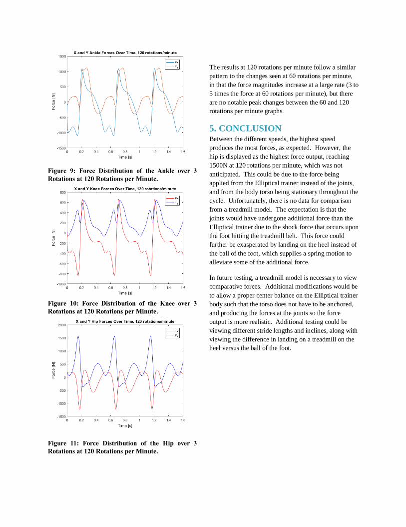
The results at 120 rotations per minute follow a similar

pattern to the changes seen at 60 rotations per minute,

in that the force magnitudes increase at a large rate (3 to

5 times the force at 60 rotations per minute), but there

are no notable peak changes between the 60 and 120

rotations per minute graphs.

5. CONCLUSION Between the different speeds, the highest speed

produces the most forces, as expected. However, the

hip is displayed as the highest force output, reaching

1500N at 120 rotations per minute, which was not

anticipated. This could be due to the force being

applied from the Elliptical trainer instead of the joints,

and from the body torso being stationary throughout the

cycle. Unfortunately, there is no data for comparison

from a treadmill model. The expectation is that the

joints would have undergone additional force than the

Elliptical trainer due to the shock force that occurs upon

the foot hitting the treadmill belt. This force could

further be exasperated by landing on the heel instead of

the ball of the foot, which supplies a spring motion to

alleviate some of the additional force.

In future testing, a treadmill model is necessary to view

comparative forces. Additional modifications would be

to allow a proper center balance on the Elliptical trainer

body such that the torso does not have to be anchored,

and producing the forces at the joints so the force

output is more realistic. Additional testing could be

viewing different stride lengths and inclines, along with

viewing the difference in landing on a treadmill on the

heel versus the ball of the foot.







References

[1] Hodgkin, Emily. "Running Myth BUSTED: The TRUTH behind Whether This Fitness Hobby Is Bad for Your Joints." Express.co.uk. Express.co.uk, 07 Feb. 2017. Web. 03 May 2017.

[2] Clauser, Charles E. "WEIGHT,

VOLUME, AND CENTER OF MASS OF

SEGMENTS OF THE HUMAN BODY." National

Technical Information Service, Aug. 1969. Web.

3 May 2017.

<http://www.dtic.mil/dtic/tr/fulltext/u2/710622.pdf

>.

MATLAB CODE

clear all;

close all;

%Gathering Data from Working Model ForceMatrix = importdata('JointForces30rotmin.dta'); ForceMatrix2 = importdata('JointForces60rotmin.dta'); ForceMatrix3 = importdata('JointForces120rotmin.dta'); t30=ForceMatrix(:,1); Ankx30 = ForceMatrix(:,2); Anky30 = ForceMatrix(:,3); Kneex30= ForceMatrix(:,6); Kneey30 = ForceMatrix(:,7); Hipx30 = ForceMatrix(:,10); Hipy30 = ForceMatrix(:,11);

t60=ForceMatrix2(:,1); Ankx60 = ForceMatrix2(:,2); Anky60 = ForceMatrix2(:,3); Kneex60= ForceMatrix2(:,6); Kneey60 = ForceMatrix2(:,7); Hipx60 = ForceMatrix2(:,10); Hipy60 = ForceMatrix2(:,11);

t120=ForceMatrix3(:,1); Ankx120 = ForceMatrix3(:,2); Anky120 = ForceMatrix3(:,3); Kneex120= ForceMatrix3(:,6); Kneey120 = ForceMatrix3(:,7); Hipx120 = ForceMatrix3(:,10); Hipy120 = ForceMatrix3(:,11);

%Plotting Data figure(1); plot(t30,Ankx30,t30,Anky30) title('X and Y Ankle Forces Over Time, 30 rotations/minute'); xlabel('Time [s]'); ylabel('Force [N]'); legend('Fx','Fy'); figure(2); plot(t30,Kneex30,'r',t30,Kneey30,'b') title('X and Y Knee Forces Over Time, 30 rotations/minute'); xlabel('Time [s]'); ylabel('Force [N]'); legend('Fx','Fy'); figure(3); plot(t30,Hipx30,'r',t30,Hipy30,'b') title('X and Y Hip Forces Over Time, 30 rotations/minute'); xlabel('Time [s]'); ylabel('Force [N]'); legend('Fx','Fy');

figure(4); plot(t60,Ankx60,t60,Anky60)

title('X and Y Ankle Forces Over Time, 60 rotations/minute'); xlabel('Time [s]'); ylabel('Force [N]'); legend('Fx','Fy'); figure(5); plot(t60,Kneex60,'r',t60,Kneey60,'b') title('X and Y Knee Forces Over Time, 60 rotations/minute'); xlabel('Time [s]'); ylabel('Force [N]'); legend('Fx','Fy'); figure(6); plot(t60,Hipx60,'r',t60,Hipy60,'b') title('X and Y Hip Forces Over Time, 60 rotations/minute'); xlabel('Time [s]'); ylabel('Force [N]'); legend('Fx','Fy');

figure(7); plot(t120,Ankx120,t120,Anky120) title('X and Y Ankle Forces Over Time, 120 rotations/minute'); xlabel('Time [s]'); ylabel('Force [N]'); legend('Fx','Fy'); figure(8); plot(t120,Kneex120,'r',t120,Kneey120,'b') title('X and Y Knee Forces Over Time, 120 rotations/minute'); xlabel('Time [s]'); ylabel('Force [N]'); legend('Fx','Fy'); figure(9); plot(t120,Hipx120,'r',t120,Hipy120,'b') title('X and Y Hip Forces Over Time, 120 rotations/minute'); xlabel('Time [s]'); ylabel('Force [N]'); legend('Fx','Fy');

Hilmi Entabi ME 581 5/3/2017

ME581 Final Project

Automotive Suspension Modeling

Automotive suspension systems are critical components of automobiles and play a significant

role in the performance of the car and comfort of the occupants. Modern suspension systems

consist of often complex geometry and 3D kinematic chains. To design suspensions that achieve

their performance goals engineers must rely on extensive modeling to understand the dynamic

relationships between the road, the vehicle tire, and the vehicle body.

Two common types of front suspension in cars are double wishbone suspensions and MacPherson Strut

suspensions. They both hold particular advantages and disadvantages based on their application. The

MacPherson Strut’s overriding advantage is its simplicity, requiring relatively few components, and its small

packaging space requirements. These factors make it an inexpensive suspension that can easily be

implemented in a broad range of vehicles. The MacPherson Strut does however have some drawbacks in

performance inherent in the design. Due to the simplicity that benefits it in cost and packaging space, its

kinematics are limited.

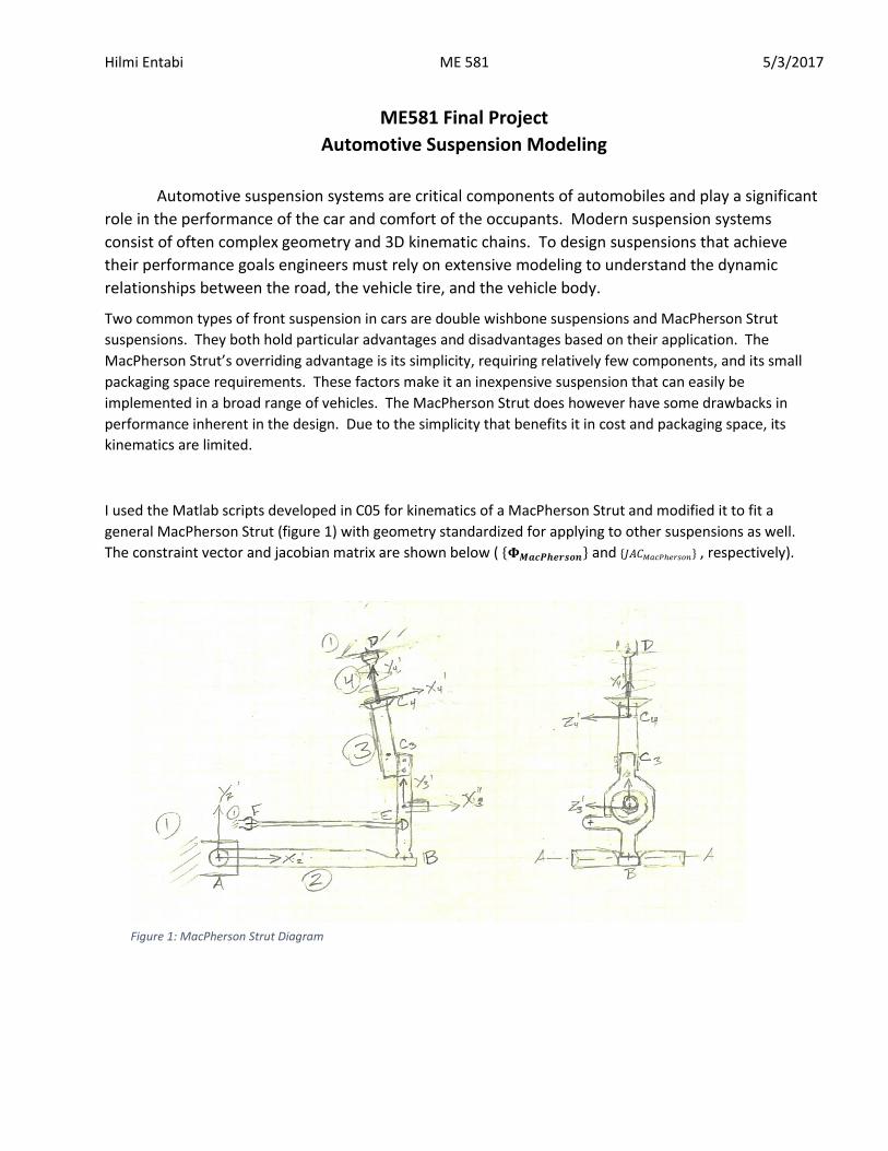
I used the Matlab scripts developed in C05 for kinematics of a MacPherson Strut and modified it to fit a

general MacPherson Strut (figure 1) with geometry standardized for applying to other suspensions as well.

The constraint vector and jacobian matrix are shown below ( {𝚽𝑴𝒂𝒄𝑷𝒉𝒆𝒓𝒔𝒐𝒏} and {𝐽𝐴𝐶𝑀𝑎𝑐𝑃ℎ𝑒𝑟𝑠𝑜𝑛} , respectively).

Figure 1: MacPherson Strut Diagram


{𝚽𝑴𝒂𝒄𝑷𝒉𝒆𝒓𝒔𝒐𝒏} =

{

{𝒓𝟏}𝑨 − {𝒓𝟐}

𝑨

{�̂�𝟐}𝑻{�̂�𝟏}

{�̂�𝟐}𝑻{�̂�𝟏}

{𝒓𝟐}𝑩 − {𝒓𝟑}

𝑩

{𝒅𝑬𝑭}𝑻{𝒅𝑬𝑭} − 𝑳

𝟐, {𝒅𝑬𝑭} = {𝒓𝟏}𝑭 − {𝒓𝟑}

𝑬

{�̂�𝟑}𝑻{�̂�𝟒}

{�̂�𝟑}𝑻{�̂�𝟒}

{�̂�𝟒}𝑻{𝒅𝑪𝟑𝑪𝟒}, {𝒅𝑪𝟑𝑪𝟒} = {𝒓𝟒}

𝑪𝟒 − {𝒓𝟑}𝑪𝟑

{�̂�𝟒}𝑻{𝒅𝑪𝟑𝑪𝟒}, {𝒅𝑪𝟑𝑪𝟒} = {𝒓𝟒}

𝑪𝟒 − {𝒓𝟑}𝑪𝟑

{�̂�𝟑}𝑻{�̂�𝟒}

{𝒓𝟏}𝑫 − {𝒓𝟒}

𝑫

{𝒑𝟐}𝑻{𝒑𝟐} − 𝟏

{𝒑𝟑}𝑻{𝒑𝟑} − 𝟏

{𝒑𝟒}𝑻{𝒑𝟒} − 𝟏

𝒚𝟑 − 𝒚𝟑𝑺𝑻𝑨𝑹𝑻 − ∆𝒚𝟑𝒕 }

{𝐽𝐴𝐶𝑀𝑎𝑐𝑃ℎ𝑒𝑟𝑠𝑜𝑛} =

[ −[𝐼3]

01×301×3

[𝐼3]01×301×3

01×301×301×3

01×303×301×301×301×301×3

2[𝐴2][𝑠2̃]′𝐴[𝐺2]

−2{ℎ1}′𝑇[𝐴1]

𝑇[𝐴2][𝑓2̃]′[𝐺2]

−2{ℎ1}′𝑇[𝐴1]

𝑇[𝐴2][𝑔2̃]′[𝐺2]

−2[𝐴2][𝑠2̃]′𝐵[𝐺2]

01×401×4

01×401×4

01×401×4

03×42{𝑝2}

𝑇

01×401×401×4

03×301×301×3−[𝐼3]

−2{𝑑𝐸𝐹}𝑇

01×3

01×3−{𝑓3}

′𝑇[𝐴3]𝑇

−{ℎ3}′𝑇[𝐴3]

𝑇

01×3

03×301×301×301×3

[0 1 0]

03×401×401×4

2[𝐴3][𝑠3̃]′𝐵[𝐺3]

4{𝑑𝐸𝐹}𝑇[𝐴3][𝑠3̃]

′𝐸[𝐺3]

−2{𝑔4}′𝑇[𝐴4]

𝑇[𝐴3][𝑓3̃]′[𝐺3]

−2{𝑔4}′𝑇[𝐴4]

𝑇[𝐴3][ℎ3̃]′[𝐺3]

2({𝑓3}′𝑇[𝑠3̃]

′𝐶 − {𝑑34}𝑇[𝐴3][𝑓3̃]

′)[𝐺3]

2({ℎ3}′𝑇[𝑠3̃]

′𝐶 − {𝑑34}𝑇[𝐴3][ℎ3̃]

′)[𝐺3]

−2{ℎ4}′𝑇[𝐴4]

𝑇[𝐴3][𝑓3̃]′[𝐺3]

03×401×42{𝑝3}

𝑇

01×401×4

03×301×301×303×301×301×3

01×3{𝑓3}

′𝑇[𝐴3]𝑇

{ℎ3}′𝑇[𝐴3]

𝑇

01×3

−[𝐼3]01×301×301×301×3

03×401×401×403×401×4

−2{𝑓3}′𝑇[𝐴3]

𝑇[𝐴4][𝑔4̃]′[𝐺4]

−2{ℎ3}′𝑇[𝐴3]

𝑇[𝐴4][𝑔4̃]′[𝐺4]

−2{𝑓3}′𝑇[𝐴3]

𝑇[𝐴4][𝑠4̃]′𝐶[𝐺4]

−2{ℎ3}′𝑇[𝐴3]

𝑇[𝐴4][𝑠4̃]′𝐶[𝐺4]

−2{𝑓3}′𝑇[𝐴3]

𝑇[𝐴4][ℎ4̃]′[𝐺4]

−2[𝐴4][𝑠4̃]′𝐷[𝐺4]

01×401×4

2{𝑝4}𝑇

01×4 ]


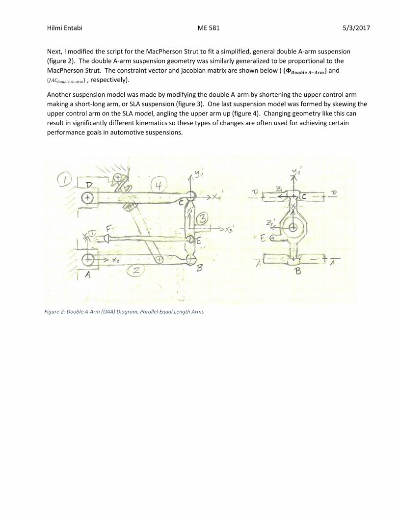
Next, I modified the script for the MacPherson Strut to fit a simplified, general double A-arm suspension

(figure 2). The double A-arm suspension geometry was similarly generalized to be proportional to the

MacPherson Strut. The constraint vector and jacobian matrix are shown below ( {𝚽𝑫𝒐𝒖𝒃𝒍𝒆 𝑨−𝑨𝒓𝒎} and

{𝐽𝐴𝐶𝐷𝑜𝑢𝑏𝑙𝑒 𝐴−𝐴𝑟𝑚} , respectively).

Another suspension model was made by modifying the double A-arm by shortening the upper control arm

making a short-long arm, or SLA suspension (figure 3). One last suspension model was formed by skewing the

upper control arm on the SLA model, angling the upper arm up (figure 4). Changing geometry like this can

result in significantly different kinematics so these types of changes are often used for achieving certain

performance goals in automotive suspensions.

Figure 2: Double A-Arm (DAA) Diagram, Parallel Equal Length Arms


{𝚽𝑫𝒐𝒖𝒃𝒍𝒆 𝑨−𝑨𝒓𝒎} =

{

{𝒓𝟏}𝑨 − {𝒓𝟐}

𝑨

{�̂�𝟐}𝑻{�̂�𝟏}

{�̂�𝟐}𝑻{�̂�𝟏}

{𝒓𝟐}𝑩 − {𝒓𝟑}

𝑩

{𝒅𝑬𝑭}𝑻{𝒅𝑬𝑭} − 𝑳

𝟐, {𝒅𝑬𝑭} = {𝒓𝟏}𝑭 − {𝒓𝟑}

𝑬

{𝒓𝟑}𝑪 − {𝒓𝟒}

𝑪

{𝒓𝟏}

𝑫 − {𝒓𝟒}𝑫

{�̂�𝟒}𝑻{�̂�𝟏}

{�̂�𝟒}𝑻{�̂�𝟏}

{𝒑𝟐}𝑻{𝒑𝟐} − 𝟏

{𝒑𝟑}𝑻{𝒑𝟑} − 𝟏

{𝒑𝟒}𝑻{𝒑𝟒} − 𝟏

𝒚𝟑 − 𝒚𝟑𝑺𝑻𝑨𝑹𝑻 − ∆𝒚𝟑𝒕 }

{𝐽𝐴𝐶𝐷𝑜𝑢𝑏𝑙𝑒 𝐴−𝐴𝑟𝑚} =

[ −[𝐼3]01×301×3[𝐼3]

01×303×3

03×301×301×301×301×301×301×3

2[𝐴2][𝑠2̃]′𝐴[𝐺2]

−2{ℎ1}′𝑇[𝐴1]

𝑇[𝐴2][𝑓2̃]′[𝐺2]

−2{ℎ1}′𝑇[𝐴1]

𝑇[𝐴2][𝑔2̃]′[𝐺2]

−2[𝐴2][𝑠2̃]′𝐵[𝐺2]

01×403×4

03×401×4

01×42{𝑝2}

𝑇

01×401×401×4

03×3

01×301×3−[𝐼3]

−2{𝑑𝐸𝐹}𝑇

[𝐼3]03×301×3

01×301×301×301×3

[0 1 0]

03×401×401×4

2[𝐴3][𝑠3̃]′𝐵[𝐺3]

4{𝑑𝐸𝐹}𝑇[𝐴3][𝑠3̃]

′𝐸[𝐺3]

−2[𝐴3][𝑠3̃]′𝐶[𝐺3]

03×401×4

01×401×42{𝑝3}

𝑇

01×401×4

03×301×301×303×301×3−[𝐼3]

−[𝐼3]01×3

01×301×301×301×301×3

03×401×401×403×401×4

2[𝐴4][𝑠4̃]′𝐶[𝐺4]

2[𝐴4][𝑠4̃]′𝐷[𝐺4]

−2{ℎ1}′𝑇[𝐴1]

𝑇[𝐴4][𝑓1̃]′[𝐺4]

−2{ℎ1}′𝑇[𝐴1]

𝑇[𝐴4][𝑔1̃]′[𝐺4]

01×401×4

2{𝑝4}𝑇

01×4 ]


Figure 3: Short-Long Arm Suspension Diagram (DAA with parallel, unequal length arms)

Figure 4: SLA-Skewed Suspension Diagram (unequal length, non-parallel arms)


Appendix A: Matlab Script for MacPherson Strut

% McP_main.m - MCPherson Strut 3D

% main

% initialize

clear all

clc

McP_ini;

McP_kin;

% one crank revolution

tpr = 3*pi/2; % time for one cycle

% timer loop

keep = [];

for t = pi/2 : pi/12 : tpr,

% kinematics

McP_kin;

% save kinematics

x = r3(1)-10;

y = r3(2)-3;

toe = asin(h3(1));

cambera = asin(f3(2));

camberx = f3(1);

cambery = f3(2);

keep = [keep; t x y chi2 toe cambera camberx cambery];

% bottom of timer loop

end

time = keep(:,1);

x = keep(:,2);

y = keep(:,3);

chi2 = keep(:,4)/d2r;

toe = keep(:,5)/d2r;

cambera = keep(:,6)/d2r;

camberx = keep(:,7);

cambery = keep(:,8);

figure(1)

hold on

grid on

plot(y, toe, 'r')

xlabel('Relative Height Above Resting Position [in]')

ylabel('Toe Angle [deg] - Positive OUT, Negative IN')

title( 'Toe Angle vs Suspension Height')

% axis equal

figure(2)

subplot(1,4,1)

hold on

grid on

scale = 0;


quiver(x, y, camberx, cambery, scale, 'r')

plot(x, y, 'ro')

%xlabel('x-Position of Knuckle')

ylabel('y-Position of Knuckle')

title({'';'MacPherson Strut'})

axis ([-1 1 -2.5 2.5])

% axis equal

figure(3)

hold on

grid on

plot(y, cambera, 'r')

xlabel('Relative Height Above Resting Position [in]')

ylabel('Camber Angle [deg] - Positive UP, Negative DOWN')

title( 'Camber Angle Angle vs Suspension Height')

%axis equal

% McP_ini.m - McPherson Strut

% initialize constants and assembly guesses

% general constants

d2r = pi / 180;

R = [ 0 -1; 1 0 ];

f = [1; 0; 0];

g = [0; 1; 0];

h = [0; 0; 1];

% mechanism constants inches

s1pA = [0; 0; 0];

s1pD = [8.00; 12.00; 0];

s1pF = [2.00; 2.00; 2.00];

s2pA = [ 0 0 0]';

s2pB = [ 10.00 0 0]';

s3pB = [ 0 -3.00 0]';

s3pC = [ -1.00 3.00 0]';

s3pE = [ 0 -1.00 2.00]';

s4pC = [ 0 0 0]';

s4pD = [ 0 3.00 0 ]';

s2pAskew = [0 -s2pA(3) s2pA(2); s2pA(3) 0 -s2pA(1); -s2pA(2) s2pA(1) 0];

s2pBskew = [0 -s2pB(3) s2pB(2); s2pB(3) 0 -s2pB(1); -s2pB(2) s2pB(1) 0];

s3pBskew = [0 -s3pB(3) s3pB(2); s3pB(3) 0 -s3pB(1); -s3pB(2) s3pB(1) 0];

s3pCskew = [0 -s3pC(3) s3pC(2); s3pC(3) 0 -s3pC(1); -s3pC(2) s3pC(1) 0];

s3pEskew = [0 -s3pE(3) s3pE(2); s3pE(3) 0 -s3pE(1); -s3pE(2) s3pE(1) 0];

s4pCskew = [0 -s4pC(3) s4pC(2); s4pC(3) 0 -s4pC(1); -s4pC(2) s4pC(1) 0];

s4pDskew = [0 -s4pD(3) s4pD(2); s4pD(3) 0 -s4pD(1); -s4pD(2) s4pD(1) 0];

EF = 8.00;


% initial guesses - angles measured by protractor

chi2 = 0*d2r;

chi3 = 10*d2r;

chi4 = chi3;

% r2

q(1,1) = 0;

q(2,1) = 0;

q(3,1) = 0;

% p2

q(4,1) = cos(chi2/2);

q(5,1) = 0;

q(6,1) = 0;

q(7,1) = sin(chi2/2);

% r3

q(8,1) = 10.00; % AB*cos(chi2)-BG*sin(chi3);

q(9,1) = 3.00; % AB*sin(chi2)+BG*cos(chi3);

q(10,1) = 0;

% p3

q(11,1) = cos(chi3/2);

q(12,1) = 0;

q(13,1) = 0;

q(14,1) = sin(chi3/2);

% r4

q(15,1) = 8.50; % q(8,1)-GC4*sin(chi4);

q(16,1) = 9.00; % q(9,1)+GC4*cos(chi4);

q(17,1) = 0;

% p4

q(18,1) = cos(chi4/2);

q(19,1) = 0;

q(20,1) = 0;

q(21,1) = sin(chi4/2);

% driver for crank - r4C-r3C = Strut_Start + jounce_dot*t

y3_start = 3.17; % Strut Jounce Start

strut_start = y3_start;

y3_dot = 4;

t = 0;

% McPherson_phi.m - McPherson Strut

% evaluate constraints and Jacobian for linear distance driving constraint

% global location of local frames and rotation matrices

% Eq 2.4.4, page 33 - Eq 2.6.5, page 42

r1 = [0 0 0]';

p1 = [1 0 0 0]';

r2 = q(1:3);

p2 = q(4:7);


r3 = q(8:10);

p3 = q(11:14);

r4 = q(15:17);

p4 = q(18:21);

% phi2 = chi2;

% phi3 = chi3;

% phi4 = chi4;

A1 = [ 1 0 0; 0 1 0; 0 0 1];

A2 = 2*[ p2(1)^2+p2(2)^2-1/2 p2(2)*p2(3)-p2(1)*p2(4) p2(2)*p2(4)+p2(1)*p2(3);

p2(2)*p2(3)+p2(1)*p2(4) p2(1)^2+p2(3)^2-1/2 p2(3)*p2(4)-p2(1)*p2(2);

p2(2)*p2(4)-p2(1)*p2(3) p2(3)*p2(4)+p2(1)*p2(2) p2(1)^2+p2(4)^2-1/2];

A3 = 2*[ p3(1)^2+p3(2)^2-1/2 p3(2)*p3(3)-p3(1)*p3(4) p3(2)*p3(4)+p3(1)*p3(3);

p3(2)*p3(3)+p3(1)*p3(4) p3(1)^2+p3(3)^2-1/2 p3(3)*p3(4)-p3(1)*p3(2);

p3(2)*p3(4)-p3(1)*p3(3) p3(3)*p3(4)+p3(1)*p3(2) p3(1)^2+p3(4)^2-1/2];

A4 = 2*[ p4(1)^2+p4(2)^2-1/2 p4(2)*p4(3)-p4(1)*p4(4) p4(2)*p4(4)+p4(1)*p4(3);

p4(2)*p4(3)+p4(1)*p4(4) p4(1)^2+p4(3)^2-1/2 p4(3)*p4(4)-p4(1)*p4(2);

p4(2)*p4(4)-p4(1)*p4(3) p4(3)*p4(4)+p4(1)*p4(2) p4(1)^2+p4(4)^2-1/2];

f1 = f;

g1 = g;

h1 = h;

f2 = A2*f;

g2 = A2*g;

h2 = A2*h;

f3 = A3*f;

g3 = A3*g;

h3 = A3*h;

f4 = A4*f;

g4 = A4*g;

h4 = A4*h;

fpskew = [0 -f(3) f(2); f(3) 0 -f(1); -f(2) f(1) 0];

gpskew = [0 -g(3) g(2); g(3) 0 -g(1); -g(2) g(1) 0];

hpskew = [0 -h(3) h(2); h(3) 0 -h(1); -h(2) h(1) 0];

G2 = [-p2(2) p2(1) p2(4) -p2(3); -p2(3) -p2(4) p2(1) p2(2); -p2(4) p2(3) -p2(2)

p2(1)];

G3 = [-p3(2) p3(1) p3(4) -p3(3); -p3(3) -p3(4) p3(1) p3(2); -p3(4) p3(3) -p3(2)

p3(1)];

G4 = [-p4(2) p4(1) p4(4) -p4(3); -p4(3) -p4(4) p4(1) p4(2); -p4(4) p4(3) -p4(2)

p4(1)];

y3 = r3(2);

% global locations - Eq 2.4.8, page 33

r1A = r1 + A1*s1pA;

r1D = r1 + A1*s1pD;

r1F = r1 + A1*s1pF;

r2A = r2 + A2*s2pA;

r2B = r2 + A2*s2pB;

r3B = r3 + A3*s3pB;

r3C = r3 + A3*s3pC;

r3E = r3 + A3*s3pE;


r4C = r4 + A4*s4pC;

r4D = r4 + A4*s4pD;

dCC = r4C-r3C;

dEF = r1F-r3E;

PHI = zeros(21,1);

% Joint A - Revolute

PHI(1:3) = r1A - r2A;

PHI(4) = f2'*h1;

PHI(5) = g2'*h1;

% Joint B - Spherical

PHI(6:8) = r2B - r3B;

% Joint E - Double Spherical (Steering Tie Rod)

PHI(9) = dEF'*dEF-EF*EF;

% Joint C - Prismatic

PHI(10) = f3'*g4;

PHI(11) = h3'*g4;

PHI(12) = f3'*dCC;

PHI(13) = h3'*dCC;

PHI(14) = f3'*h4;

% Joint D - Spherical

PHI(15:17) = r1D - r4D;

% Euler Parameters

PHI(18) = p2'*p2-1;

PHI(19) = p3'*p3-1;

PHI(20) = p4'*p4-1;

% vertical translation driving constraint

PHI(21) = y3 - y3_start - 2*sin(t);

% Jacobian by rows - Eq 3.3.12, page 66 for revolutes

JAC = zeros(21,21);

% Joint A - Revolute

JAC(1:3,1:3) = -eye(3); JAC(1:3,4:7)=2*A2*s2pAskew*G2;

JAC(4,4:7) = -2*h'*A1'*A2*fpskew*G2;

JAC(5,4:7) = -2*h'*A1'*A2*gpskew*G2;

% Joint B - Spherical

JAC(6:8,1:3) = eye(3); JAC(6:8,4:7) = -2*A2*s2pBskew*G2;

JAC(6:8,8:10) = -eye(3); JAC(6:8,11:14) = 2*A3*s3pBskew*G3;

% Joint E - Double Revolute

JAC(9,8:10) = -2*dEF'; JAC(9,11:14) = 4*dEF'*A3*s3pEskew*G3;

% Joint C - Prismatic

JAC(10,11:14) = -2*g'*A4'*A3*fpskew*G3; JAC(10,18:21) = -2*f'*A3'*A4*gpskew*G4;

JAC(11,11:14) = -2*g'*A4'*A3*hpskew*G3; JAC(11,18:21) = -2*h'*A3'*A4*gpskew*G4;


JAC(12,8:10) = -f'*A3'; JAC(12,11:14) = 2*(f'*s3pCskew-

dCC'*A3*fpskew)*G3;

JAC(12,15:17) = f'*A3'; JAC(12,18:21) = -2*f'*A3'*A4*s4pCskew*G4;

JAC(13,8:10) = -h'*A3'; JAC(13,11:14) = 2*(h'*s3pCskew-

dCC'*A3*hpskew)*G3;

JAC(13,15:17) = h'*A3'; JAC(13,18:21) = -2*h'*A3'*A4*s4pCskew*G4;

JAC(14,11:14) = -2*h'*A4'*A3*fpskew*G3; JAC(14,18:21) = -2*f'*A3'*A4*hpskew*G4;

% Joint D - Spherical

JAC(15:17,15:17) = -eye(3); JAC(15:17,18:21) = 2*A4*s4pDskew*G4;

JAC(18,4:7) = 2*p2';

JAC(19,11:14) = 2*p3';

JAC(20,18:21) = 2*p4';

% driving constraint in Jacobian - Eq 3.1.9, page 52

JAC(21,8:10) = [0 1 0];

% McP_kin.m - MCPherson Strut 3D % positon, velocity, and acceleration at desired_crank

% Newton-Raphson position solution - Eq 3.6.7 and 3.6.8, page 100 assy_tol = 0.00001; McP_phi; while max(abs(PHI)) > assy_tol, q = q - inv(JAC) * PHI; McP_phi; end


Appendix B: Matlab Script for Double A-Arm Kinematics

% DAA_main.m - Double A-Arm Suspension Main

% initialize clear all clc DAA_ini; DAA_kin;

tpr = 3*pi/2; % time for one cycle

% timer loop keep = []; for t = pi/2 : pi/12 : tpr,

% kinematics DAA_kin;

% save kinematics x = r3(1)-10; y = r3(2)-3; toe = asin(h3(1)); cambera = asin(f3(2)); camberx = f3(1); cambery = f3(2);

keep = [keep; t x y chi2 toe cambera camberx cambery];

% bottom of timer loop end

time = keep(:,1); x = keep(:,2); y = keep(:,3); chi2 = keep(:,4)/d2r; toe = keep(:,5)/d2r; cambera = keep(:,6)/d2r; camberx = keep(:,7); cambery = keep(:,8);

figure(1) hold on plot(y, toe, 'b') xlabel('Relative Height Above Resting Position [in]') ylabel('Toe Angle [deg] - Positive OUT, Negative IN') title( 'Toe Angle vs Suspension Height') %axis equal

figure(2) subplot(1,4,2) hold on grid on scale = 0; quiver(x, y,camberx, cambery, scale, 'b')


hold on plot(x, y, 'bo') xlabel('x-Position of Knuckle') %ylabel('y-Position of Knuckle') title({'Knuckle Position & Spindle Axis Direction';'Double A-Arm'}) axis ([-1 1 -2.5 2.5]) hold off %axis equal

figure(3) hold on grid on plot(y, cambera, 'b') xlabel('Relative Height Above Resting Position [in]') ylabel('Camber Angle [deg] - Positive UP, Negative DOWN') title( 'Camber Angle Angle vs Suspension Height') %axis equal

% DAA_ini.m - Double A-Arm Suspension % initialize constants and assembly guesses

% general constants d2r = pi / 180;

f = [1; 0; 0]; g = [0; 1; 0]; h = [0; 0; 1];

% mechanism constants

% Parallel, Equal Length Upper & Lower Arms s1pA = [0; 0; 0]; s1pD = [0; 6.00; 0]; s1pF = [2.00; 2.00; 2.00];

s2pA = [ 0 0 0]'; s2pB = [ 10.00 0 0]';

s3pB = [ 0 -3.00 0]'; s3pC = [ 0 3.00 0]'; s3pE = [ 0 -1.00 2.00]';

s4pC = [ 0 0 0]'; s4pD = [ -10.00 0 0 ]';

%---------------------------------------------------------------------

s2pAskew = [0 -s2pA(3) s2pA(2); s2pA(3) 0 -s2pA(1); -s2pA(2) s2pA(1) 0]; s2pBskew = [0 -s2pB(3) s2pB(2); s2pB(3) 0 -s2pB(1); -s2pB(2) s2pB(1) 0];

s3pBskew = [0 -s3pB(3) s3pB(2); s3pB(3) 0 -s3pB(1); -s3pB(2) s3pB(1) 0]; s3pCskew = [0 -s3pC(3) s3pC(2); s3pC(3) 0 -s3pC(1); -s3pC(2) s3pC(1) 0]; s3pEskew = [0 -s3pE(3) s3pE(2); s3pE(3) 0 -s3pE(1); -s3pE(2) s3pE(1) 0];


s4pCskew = [0 -s4pC(3) s4pC(2); s4pC(3) 0 -s4pC(1); -s4pC(2) s4pC(1) 0]; s4pDskew = [0 -s4pD(3) s4pD(2); s4pD(3) 0 -s4pD(1); -s4pD(2) s4pD(1) 0];

EF = 8.00;

% initial guesses - angles measured by protractor chi2 = 0*d2r; chi3 = 0*d2r; chi4 = 0*d2r;

% r2 q(1,1) = 0; q(2,1) = 0; q(3,1) = 0;

% p2 q(4,1) = cos(chi2/2); q(5,1) = 0; q(6,1) = 0; q(7,1) = sin(chi2/2);

% r3 q(8,1) = 10.00; % AB*cos(chi2)-BG*sin(chi3); q(9,1) = 3.00; % AB*sin(chi2)+BG*cos(chi3); q(10,1) = 0;


% r4 q(15,1) = 10.00; % q(8,1)-GC4*sin(chi4); q(16,1) = 6.00; % q(9,1)+GC4*cos(chi4); q(17,1) = 0;


% driver for crank - r4C-r3C = Strut_Start + jounce_dot*t y3_start = 3; % Strut Jounce Start t = 0;

% DAA_phi.m - Double A-Arm Suspension % evaluate constraints and Jacobian for linear distance driving constraint

% global location of local frames and rotation matrices % Eq 2.4.4, page 33 - Eq 2.6.5, page 42 r1 = [0 0 0]';


p1 = [1 0 0 0]';

r2 = q(1:3); p2 = q(4:7);

r3 = q(8:10); p3 = q(11:14);

r4 = q(15:17); p4 = q(18:21);

A1 = [ 1 0 0; 0 1 0; 0 0 1]; A2 = 2*[ p2(1)^2+p2(2)^2-1/2 p2(2)*p2(3)-p2(1)*p2(4) p2(2)*p2(4)+p2(1)*p2(3); p2(2)*p2(3)+p2(1)*p2(4) p2(1)^2+p2(3)^2-1/2 p2(3)*p2(4)-p2(1)*p2(2); p2(2)*p2(4)-p2(1)*p2(3) p2(3)*p2(4)+p2(1)*p2(2) p2(1)^2+p2(4)^2-1/2]; A3 = 2*[ p3(1)^2+p3(2)^2-1/2 p3(2)*p3(3)-p3(1)*p3(4) p3(2)*p3(4)+p3(1)*p3(3); p3(2)*p3(3)+p3(1)*p3(4) p3(1)^2+p3(3)^2-1/2 p3(3)*p3(4)-p3(1)*p3(2); p3(2)*p3(4)-p3(1)*p3(3) p3(3)*p3(4)+p3(1)*p3(2) p3(1)^2+p3(4)^2-1/2]; A4 = 2*[ p4(1)^2+p4(2)^2-1/2 p4(2)*p4(3)-p4(1)*p4(4) p4(2)*p4(4)+p4(1)*p4(3); p4(2)*p4(3)+p4(1)*p4(4) p4(1)^2+p4(3)^2-1/2 p4(3)*p4(4)-p4(1)*p4(2); p4(2)*p4(4)-p4(1)*p4(3) p4(3)*p4(4)+p4(1)*p4(2) p4(1)^2+p4(4)^2-1/2]; f1 = f; g1 = g; h1 = h; f2 = A2*f; g2 = A2*g; h2 = A2*h; f3 = A3*f; g3 = A3*g; h3 = A3*h; f4 = A4*f; g4 = A4*g; h4 = A4*h;

fpskew = [0 -f(3) f(2); f(3) 0 -f(1); -f(2) f(1) 0]; gpskew = [0 -g(3) g(2); g(3) 0 -g(1); -g(2) g(1) 0]; hpskew = [0 -h(3) h(2); h(3) 0 -h(1); -h(2) h(1) 0];

G2 = [-p2(2) p2(1) p2(4) -p2(3); -p2(3) -p2(4) p2(1) p2(2); -p2(4) p2(3) -p2(2)

p2(1)]; G3 = [-p3(2) p3(1) p3(4) -p3(3); -p3(3) -p3(4) p3(1) p3(2); -p3(4) p3(3) -p3(2)

p3(1)]; G4 = [-p4(2) p4(1) p4(4) -p4(3); -p4(3) -p4(4) p4(1) p4(2); -p4(4) p4(3) -p4(2)

p4(1)];

y3 = r3(2);

% global locations - Eq 2.4.8, page 33 r1A = r1 + A1*s1pA; r1D = r1 + A1*s1pD; r1F = r1 + A1*s1pF;

r2A = r2 + A2*s2pA; r2B = r2 + A2*s2pB;


r3B = r3 + A3*s3pB; r3C = r3 + A3*s3pC; r3E = r3 + A3*s3pE;

r4C = r4 + A4*s4pC; r4D = r4 + A4*s4pD;

dCC = r4C-r3C; dEF = r1F-r3E;

PHI = zeros(21,1);

% Joint A - Revolute PHI(1:3) = r1A - r2A; PHI(4) = f2'*h1; PHI(5) = g2'*h1;

% Joint B - Spherical PHI(6:8) = r2B - r3B;

% Joint E - Double Spherical (Steering Tie Rod) PHI(9) = dEF'*dEF-EF*EF;

% Joint C - Spherical PHI(10:12) = r3C - r4C;

% Joint D - Revolute PHI(13:15) = r1D - r4D; PHI(16) = f4'*h1; PHI(17) = g4'*h1;

% Euler Parameters PHI(18) = p2'*p2-1; PHI(19) = p3'*p3-1; PHI(20) = p4'*p4-1;

% vertical translation driving constraint PHI(21) = y3 - y3_start - 2*sin(t);

% Jacobian by rows - Eq 3.3.12, page 66 for revolutes JAC = zeros(21,21);

% Joint A - Revolute JAC(1:3,1:3) = -eye(3); JAC(1:3,4:7)=2*A2*s2pAskew*G2; JAC(4,4:7) = -2*h'*A1'*A2*fpskew*G2; JAC(5,4:7) = -2*h'*A1'*A2*gpskew*G2;

% Joint B - Spherical JAC(6:8,1:3) = eye(3); JAC(6:8,4:7) = -2*A2*s2pBskew*G2; JAC(6:8,8:10) = -eye(3); JAC(6:8,11:14) = 2*A3*s3pBskew*G3;

% Joint E - Double Revolute JAC(9,8:10) = -2*dEF'; JAC(9,11:14) = 4*dEF'*A3*s3pEskew*G3;


% Joint C - Spherical JAC(10:12,8:10) = eye(3); JAC(10:12,11:14) = -2*A3*s3pCskew*G3; JAC(10:12,15:17) = -eye(3); JAC(10:12,18:21) = 2*A4*s4pCskew*G4;

% Joint D - Revolute JAC(13:15,15:17) = -eye(3); JAC(13:15,18:21)=2*A4*s4pDskew*G4; JAC(16,18:21) = -2*h'*A1'*A4*fpskew*G4; JAC(17,18:21) = -2*h'*A1'*A4*gpskew*G4;

% Euler Parameters JAC(18,4:7) = 2*p2'; JAC(19,11:14) = 2*p3'; JAC(20,18:21) = 2*p4';

% driving constraint in Jacobian - Eq 3.1.9, page 52 JAC(21,8:10) = [0 1 0];

% SLA_kin.m - Short-Long Arm Suspension % positon, velocity, and acceleration at desired position

% Newton-Raphson position solution - Eq 3.6.7 and 3.6.8, page 100 assy_tol = 0.00001; DAA_phi; while max(abs(PHI)) > assy_tol, q = q - inv(JAC) * PHI; DAA_phi; end

1


Systems Development of a Forward Dynamic

Simulation for a Lower Body

Musculoskeletal Model: A Loaded Ankle

Extension Task

Lauren Hickox

Abstract

Musculoskeletal geometry of the human body

affects how people move and how efficiently they

move. For this project, a musculoskeletal model

of the lower limb was developed in Simscape

Multibody and run using MATLAB to investigate

the effect of foot structure and musculotendon

properties on performance and energy efficiency in

a loaded ankle extension task. A test case was

simulated and a sensitivity analysis was performed

that suggested shorter heels (plantarflexor moment

arms) may increase energy efficiency during

certain movements. The simulation was also used

to design a corresponding experiment that will be

used for further exploration and validation of the

model.

2. Introduction

Energy efficiency is an important factor in human

locomotion and understanding how humans take

advantage of the geometry and properties of their

musculoskeletal system to increase this efficiency

has many applications ranging from prosthetic and

exoskeleton design to surgery to performance

training for elite athletes. A main area currently

under study is moment arms about different joints

in the body, particularly the ankle (due to its

importance in locomotion). The heel length

determines the moment arm between the

plantarflexor and the ankle while the toe length

determines the approximate moment arm between

the ground reaction force and the ankle.

Studies have suggested that these moment arms

affect the performance and efficiency of different

movements. For example, sprinters have been

shown to have longer toes and shorter heels than

the general population [1,2]. The longer toes

provide more contact time with the ground for the

plantarflexors to develop force. The shorter heels

allow the plantarflexor muscle to operate in a more

optimal location on the force-length and force-

velocity curves that govern the force production

capabilities of muscles shown in Figure 1(a) and

1(b). A shorter heel requires a smaller length

change and lower velocity of muscle for the same

ankle motion, increasing the amount of force that

can be produced.

It has also been found in a study by Scholz, et al.

that running economy increases with shorter heels

[4]. The suggested explanation was based on the

spring-like behavior of the tendon as represented

in the Hill-type muscle model (Figure 1(c)).

Figure 1: Characteristics of the (a) muscle force-

length relationship, (b) muscle force-velocity

relationship, and (c) tendon force-length

relationship and (d) diagram of a Hill-type muscle

model with a contractile element CE in series with

an elastic tendon element [3].

2

Tendons operate on a force-length curve as shown

in Figure 1(d). Therefore, the greater plantarflexor

force required to produce the same ankle moment

with shorter heels increases the strain on the

tendon. The further the tendon stretches, the more

energy it stores and then later returns, reducing the

amount of energy that the muscles need to

generate. However, a following study by van

Werkhoven did not find this shorter heel-energy

efficiency relationship. While energy storage may

increase, there will also be an increase in

metabolic cost due to the greater amount of

required force and muscle activation [5].

So far, studies have had inconsistent results on

which effect dominates. In order to further explore

the effect of foot structure on performance and

energy efficiency in humans, a musculoskeletal

simulation of the lower limb was developed for

this project.

3. Methodology

3.1. Simulation Design

Main considerations in the simulation design were

that it (1) be a single-joint motion that focuses on

the plantarflexor musclulotendon complex and

minimizes the contribution of other muscles, (2)

has a clear objective that can be measured, and (3)

allows for a good comparison with experimental

work. The task chosen for the simulation was a

loaded ankle extension (Figure 2). The objective

of the task was to push a load up an incline. The

load, distance the load was pushed, and angle of

the incline determine the work done on the load.

In an experiment, the mass of the load or load

application point could be varied in order to

change the force transferred to the plantarflexors.

The use of a simulation adds the ability to control

internal variables, such as heel moment arm and

muscle and tendon properties.

Figure 2: Experimental concept for the loaded ankle

extension task showing heel (r) and toe (R) moment

arms.

3.2. Musculoskeletal Model

A simple musculoskeletal model of the human

body was used in this simulation to represent a

single lower limb consisting of two segments: a

foot and a lower leg. The upper leg and the rest of

body were assumed to remain stationary and the

model was constrained to the sagittal plane (only

flexion/extension of the ankle was considered).

The geometric, inertial, and tissue properties for

the model were based on average values from the

commonly used Arnold model (originally from

cadaver studies) [3]. An adaption of the Arnold

model used for previous studies in the lab (Figure

3) [6] was referenced in the development of the

current model.

Two lumped muscle-tendon units, representing the

plantarflexors (medial and lateral gastrocnemius,

soleus) and dorsiflexor (tibialis anterior) were used

to drive the model. A Hill-type muscle model was

used which included the force-length and force-

velocity relationships of the muscle, as well as the

force-length relationship of the tendon [7].

Metabolic energy rates for each muscle group

were calculated and integrated over the duration of

the simulation to determine total energy

expenditure [8].

3

Figure 3: Simple musculoskeletal model of the lower

limb [6].

3.3. Mechanism

The planar mechanism for the simulation

combined the musculoskeletal model and the

planned testing device for the ankle extension

(Figure 4). The body and the testing device were

attached to the ground (world frame) forming a

closed loop. Revolute joints were used for the

knee (world frame to lower leg) and ankle (lower

leg to foot). The load was modeled as a point

mass and attached to the toe with another revolute

joint. It was allowed to slide along the incline

with a prismatic joint that was assumed to be

frictionless. This setup resulted in a four-bar

slider crank.

Figure 4: Diagram of mechanism consisting of the

lower body musculoskeletal model and testing

device.

A mobility (M) analysis was performed on the

design using equation (1). With four links (nL =

4) and four joints that allow a single degree of

freedom (nJ1 = 4 and nJ2 = 0), the mechanism was

determined to have one degree of freedom, as

desired. A mobility analysis of an earlier version

of the design resulted in the addition of the

revolute joint at the knee (previously a weld joint)

in order to allow the mechanism to move.

(1)

3.4. Model Implementation

The model was implemented in Simscape

Multibody (Simulink, Mathworks, Natick, MA) as

shown in Figure A-1 (Appendix A). Blocks were

used to represent the different bodies and joints in

the model. Coordinate frames were set up at the

joints and centers of mass for each body as shown

in Figure 5(a). The muscle models were included

as subsystems that received input about the

position of the musculotendon attachment sites on

the foot and leg segments in the world frame

(Figure 6). This was used to calculate the current

length and velocity states of the muscles and

tendons which, along with the muscle excitation

curves, determined the force produced.

The forces were returned to the main model and

applied to the segments as tension along the

muscle paths. The muscle often does not travel

directly between attachment points on two

segments. There are physical constraints, such as

bone and soft tissue, that require a more complex

path and are modeled as via points or wrapping

surfaces. In the case of the dorsiflexor, two via

points were included on the leg segment as shown

in Figure 5(b). An example of the implementation

of the coordinate system transformations in the leg

subsystem of the model is shown in Figure A-2

(Appendix A).

4

Figure 5: Graphic representation of Simscape model

showing (a) the coordinate frames for the joints,

centers of mass, and muscle-tendon attachment and

via points and (b) the lines of action for the

plantarflexor and dorsiflexor.

Another component of the model that is required

in biological systems is limiting the range of

motion of the joints that is constrained due to

passive joint mechanics. To accomplish this, a

torsional spring was added to the ankle that started

applying torque to the joint when it went beyond

the normal range of motion (50° plantarflexion to

20° dorsiflexion) as shown in Figure 6.

Figure 6: Flow of information between muscle

models and body segments and ankle spring limiting

the range of motion.

3.5. Forward Dynamic Simulation

The forward dynamic simulation of the model was

executed in MATLAB (Mathworks, Natick, MA).

A script was used to initialize the required

parameters and positions. Variables were used for

a majority of the parameters in the Simscape

model (including the foot geometry,

musculotendon properties, mass of the load, and

angle of incline of the load path) and could be

easily changed in the script. The inputs to control

the model were muscle excitation curves for the

plantarflexor and dorsiflexor (each consisting of

11 nodes evenly spaced over the duration of the

simulation). The excitation values (representing

electrical signal to the muscles) ranged from 0 (no

excitation) to 1 (maximum excitation). After the

setup, the script called the simulation and then

read and compiled the results.

4. Simulation Results

For a test case, parameters were chosen that

created a physically reasonable movement of the

model. A mass of 20 kg, incline of 30°, and

duration of 0.5 seconds were used. Only the

plantarflexor was activated and the excitation

curve was tuned (Figure 7) so that the model

performed a semi-periodic motion (Figure 8).

(a)

(b)

positions

forces

Ankle spring

Plantarflexor line

of action

Dorsiflexor lines of

action with via points

5

Figure 7: Plantarflexor excitation curve used for the

simulation.

Figure 8: Motion of model during simulation from

initial position to full extension and back to the

approximate initial position.

The resulting kinematics and kinetics of the load

and ankle are shown in Figures 9 and 10. The load

traveled a distance of 8.52 cm along the ramp

before returning to near its original position.

The ankle covered a range of motion from 4.6°

dorsiflexion (+) to 28.5° plantarflexion (-). The

high extension torque of the ankle can be seen at

the beginning of the movement that provides a

spike in the velocity of the ankle and the load.

The high velocity of the ankle and therefore the

plantarflexor causes a decrease in possible force

production and a decrease in the torque. As the

load reaches its maximum distance and starts to

move back down the incline, the plantarflexor

muscle stays activated and works against the

gravitational force to slow the travel of the load in

order to approximate the periodic motion.

Figure 9: Position from start and velocity of load

along the incline.

Internal variables that are difficult or impossible to

currently measured in humans can also be

determined from the simulation. These variables

include the force, rate of energy consumption, and

tendon strain of the plantarflexor which are shown

in Figure 11. The force shows the same pattern as

the ankle torque (as it causes the ankle torque).

The rate of energy consumption and strain in the

tendon also follow a similar pattern as both are

dependent upon the force. The energy rate is

estimated using the activation, force, and velocity

of the muscle, with a total energy of 18.29 J

consumed by the plantarflexor. The tendon acts as

a spring and the amount of tendon strain (and

energy stored in the tendon) increases with the

force.

0 0.1 0.2 0.3 0.4 0.5

Time (s)

0

0.02

0.04

0.06

0.08

0.1

Load P

ositi

ion (

m)

0 0.1 0.2 0.3 0.4 0.5

Time (s)

-1.5

-1

-0.5

0

0.5

1

Load V

elo

city

(m

/s)

0 0.1 0.2 0.3 0.4 0.5

Time (s)

0

0.02

0.04

0.06

0.08

0.1

Load

Pos

itiio

n (m

)

0 0.1 0.2 0.3 0.4 0.5

Time (s)

-1.5

-1

-0.5

0

0.5

1

Load

Vel

ocity

(m

/s)

6

Figure 10: Kinematic and kinetic results for the

ankle joint (Plantarflexion is negative for angle and

velocity and positive for torque).

A sensitivity analysis was performed to examine

the effect of varying moment arms on performance

and energy expenditure during the ankle extension

task. The simulation was run multiple times with

small changes in the heel length. The original heel

length was 4.38 cm so 0.1 cm increments were

chosen to provide about a 2% change. An

adjustment of 1 cm in each direction was also

simulated to check if the observed relationships

held for larger changes.

Figure 11: Force production, energy rate, and

tendon strain of the plantarflexor.

For each heel length, the resulting distance

traveled by the load and estimated energy

expenditure of the plantarflexor are shown in

Figure 12. Though the differences are fairly small,

a trend towards greater distance traveled coupled

with a decrease in energy use suggests greater

energy efficiency with shorter heels. However,

this relationship needs to be explored further to

determine its dependency on other model

parameters and the setup of the testing device.

0 0.1 0.2 0.3 0.4 0.5

Time (s)

-30

-20

-10

0

10A

nkle

Ang

le [deg

]

0 0.1 0.2 0.3 0.4 0.5

Time (s)

-400

-200

0

200

400

600

Ankle

Ang

. V

elo

city [deg

/s]

0 0.1 0.2 0.3 0.4 0.5

Time (s)

0

5000

10000

15000

Ankle

Torq

ue (

Nm

)

0 0.1 0.2 0.3 0.4 0.5

Time (s)

0

2000

4000

6000

PF

Forc

e (

N)

0 0.1 0.2 0.3 0.4 0.5

Time (s)

0

50

100

150

PF

Energ

y R

ate

(J/s

)

EPF

= 18.29114 J

0 0.1 0.2 0.3 0.4 0.5

Time (s)

0

0.01

0.02

0.03

0.04

PF

Tendon S

train

7

Figure 12: Sensitivity analysis of the effect of heel

moment arm changes on performance (distance

traveled by load) and energy expenditure.

5. Conclusion

For this project, a lower limb musculoskeletal

model and simulation were developed to

investigate the effect of musculoskeletal geometry

on the performance and energy efficiency of a

simple ankle extension task. The simulation was

used for an initial exploration into the effect of

heel moment arm on performance and energy

consumption. The results support the theory that

shorter heels allow for increased energy efficiency

during human movement and suggest the need for

further study of the mechanisms behind this

potential relationship. The simulation can also be

used to study the effect of other factors, such as

optimal muscle fiber length, tendon stiffness, and

movement frequency and the interactions between

them.

The planned next step is to put the simulation into

an optimization that will determine the control

strategy (muscle excitation curves) to perform a

specific ankle extension task while minimizing

energy. The results will be compared to an

experimental study that was developed during the

process of this project to correspond as closely as

possible to the simulation. The experimental study

will also be used to help validate this model.

References

[1] Lee, S. and Piazza, S., 2009, “Built for speed:

musculoskeletal structure and sprinting

ability,” J Exp Biol, 212(22), pp. 3700-3707.

[2] Baxter, J., Novack, T., Van Werkhoven, H.,

Pennell, D., and Piazza, S., 2012, “Ankle joint

mechanics and foot proportions differ between

human sprinters and non-sprinters,” Proc. R.

Soc. B, 279(1735), pp. 2018-2024.

[3] Arnold, E., Ward, S., Lieber, R., and Delp, S.,

2010, “A model of the lower limb for analysis

of human movement,” Ann Biomed Eng, 38,

pp. 269-279.

[4] Scholz M., Bobbert, M., van Soest, A., Clark,

J., and van Heerden, J., 2008, “Running

biomechanics: shorter heels, better economy,”

J Exp Biol, 211(20), pp. 3266-3271.

[5] van Werkhoven, H., 2014, “Influence of foot

and ankle structure on optimal performance in

different motor tasks,” PhD Dissertation, The

Pennsylvania State University, PA.

[6] van Werkhoven, H, and Piazza, S., 2013,

“Computational model of maximal-height

single-joint jumping predicts bouncing as an

optimal strategy,” J Biomech, 46, pp. 1092-

1097.

[7] Schutte, L., 1992, “Using musculoskeletal

models to explore strategies for improving

performance in electrical stimulation-induced

leg cycle ergometry,” PhD Dissertation,

Stanford University, PA.

[8] Umberger, B., Gerritsen, K., and Martin, P.,

2003, “A model of human muscle energy

expenditure,” Comput Methods Biomech

Biomed Engin, 6, pp. 99-111.

8

Fig

ure

A-1

: F

ull

Sim

sca

pe

Mu

ltib

od

y m

od

el

sho

win

g s

tru

ctu

re o

f b

od

ies,

jo

ints

, a

nd

act

ua

tors

.

Appendix A

9

Fig

ure

A-2

: E

xp

an

ded

leg

su

bsy

stem

in

th

e S

imsc

ap

e M

ult

ibo

dy

mo

del

sh

ow

ing

th

e im

ple

men

tati

on

of

the

tra

nsf

orm

ati

on

s fr

om

th

e k

nee

co

ord

ina

te f

ram

e to

th

e an

kle

, ce

nte

r o

f m

ass

(C

OM

), a

nd

att

ach

men

t si

tes

an

d

via

po

ints

of

the

pla

nta

rfle

xor

(PF

) a

nd

do

rsif

lex

or

(DF

).

Fig

ure

A-2

: E

xp

an

ded

leg

su

bsy

stem

fro

m t

he

Sim

sca

pe

Mu

ltib

od

y m

od

el

sho

win

g t

he

imp

lem

en

tati

on

of

the

tra

nsf

orm

ati

on

s fr

om

th

e k

nee

co

ord

ina

te f

ram

e to

th

e fr

am

es f

or

the

cen

ter

of

ma

ss (

CO

M),

an

kle

join

t, a

nd

mu

scle

att

ach

men

t a

nd

via

po

ints

fo

r th

e p

lan

tarf

lex

or

(PF

) a

nd

do

rsif

lex

or

(DF

).


Systems Multi-Link Manipulator with Compliant

End Effector

Justin A. Jones

Introduction

According to Credence Research [1] the medical

robotic industry is valued at 7.24 billion in 2015 and

will grow to over 20 billion by 2023. It is important

that the robotic mechanism is well designed since a

poor design could be potentially life threatening.

Probably the most well-known surgical robot would

be the de Vinci system developed by Intuitive

Surgical, as seen in Figure 1 (A). These surgical

robotic systems utilize specialized end effectors to

grasp and cut in order for the physician to perform

the procedure. An example of such a design can be

seen in Figure 1(B). These rigid mechanisms

consist of multiple moving small parts. A compliant

mechanism design may provide benefits over these

rigid end effector mechanisms due to the ability to

make highly accurate mechanisms with a lower

number of parts as well as the use of micro

manufacturing process.

This report develops the forward kinematic

equations for a four degree of freedom (DOF)

robotic manipulator using Denavit-Hartenberg

(DH) convention as well as analysis of a potential

complaint end effector tool for grasping. The

kinematic analysis of the compliant gripper will

utilize Ed Haug notation. A multibody dynamic

simulation was also performed on the compliant

mechanism to determine joint stresses with respect

to the driver position.

Figure 1. (A)The da Vinci robotic assisted surgery

system developed by Intuitive Surgical [2]and (B) a

rigid body end effector used for cutting[3].

2. Methodology

2.1. Robotic Manipulator

A robotic manipulator with four revolute joints and

five links was chosen for analyses. A common

method to assign coordinate systems is that of the

Denavit-Hartenberg method [4]. This method has

four constraints that must be adhered to in order to

generate the coordinate system. They are as

follows:

1: Xn ⊥ Zn-1

2: Xn ∩ Zn-1 ≠ 0

3: Origin of joint n ∩ Xn and Zn

4: Coordinate system must be right handed.

Additionally, there are four parameters that are used

to describe the system described as follows:

an = the distance from Zn to Zn+1 along Xn

αn = the angle from Zn to Zn+1 measured

about Xn

dn = the distance from Xn-1 to Xn along

Zn

Θn = the angle from Xn-1 to Xn about Zn

The 4-DOF robotic arm consisting of four revolute

joints with the coordinate frames attached using the

DH convention can be seen in Figure 2. The

corresponding DH parameters can be seen in table

1.

A B

Figure 2 Four degree of freedom robotic manipulator

with coordinate frames using the DH convention.

Table 1 DH parameters

n α [deg] a [mm] d [mm] ϑ

1 90 0 80 ϑ1

2 0 120 50 ϑ2

3 180 45 25 ϑ3

4 0 30 0 ϑ4

The benefit of using the DH convention is that it

simplifies the transformation matrix. It is now

possible to only use the four parameters in table 1

to create a generic transformation matrix as seen in

Equation 1 [4]. This transformation matrix

describes the rotation and translation of coordinate

frame n in relation to coordinate frame n-1.

1000

0

1111

1111

1

1

nnnnnnn

nnnnnnn

nnn

n

ndccscss

dsscccs

asc

T

(1)

Once each transformation matrix between each

pair of frames in known a transformation matrix

between the base and the end effector can be

calculated using Equation 2:

TTTTT n

nn

12

3

1

2

0

1

0 ... (2)

2.1.2 Forward Kinematics

From the general transformation matrix, Equation

1, it possible to generate the transformation matrix

for each coordinate frame. Equations 3-6 are the

transformation matrix for each coordinate frame

using the parameters found in table 1.

1000

100

00

00

1

11

11

0

1d

cs

sc

T

(3)

1000

00

100

00

22

2

22

1

2

cs

d

sc

T (4)

1000

000

01

0

3

33

233

2

3d

cs

asc

T

(5)

1000

0100

00

0

44

344

3

4

cs

asc

T (6)

Finally using equation 2 the overall transformation

matrix can be developed, shown in equation 7.

1000

333231

232221

131211

0

4

z

y

x

Prrr

Prrr

Prrr

T (7)

The overall transformation matrix consists of the

rotational matrix Rij and the positional vector P. the

vector P in Equation 7 represents the global

p

z0

z2

z1

z4

x0

y0 x

2

y2

z3 x

3

y3

x1

y1

x4

y4

a2

a4

d2

d4

a3

Θ1

Θ2 Θ

3

Θ4

d1

coordinates of the arm end point P shown in Figure

2.

To check the forward kinematic equations Figures

3 and 4 show the rotation about the wrist and

shoulder joint, varying from 0 to 2π while holding

the other joints fixed.

Figure 3 Rotational position of wrist joint.

Figure 4 Rotational position of manipulator by

iterating ϑ1.

2.2. Compliant Gripper

Compliant mechanisms provide many benefits

when compared to their rigid body counter parts.

Some of these benefits include ease of

manufacturing, reduction of wear and friction, and

reduced need for lubrication [5, 6]. Additionally,

compliant mechanisms are widely used in the

manufacturing of MEMs and NEMS as well as in

photolithography. The ability to make very small

mechanisms that have reduced wear and

maintenance could prove large benefits to the

medical field, such as in the area of non-invasive

surgeries like laparoscopic surgery.

To design a complaint mechanism, at least when

only the kinematics are of concern, it is possible to

replace the flexible members with revolute joints

and treat the mechanism as a rigid body

mechanism. However, it should be noted that for

compliant mechanisms the flexible member degree

of rotation is constrained. Further, they are prone

to failure due to overstress and fatigue. For the

dynamic response of the mechanism it is possible

to use the Pseudo-Rigid-Body Model that was

developed by Howell and Midha [7]. They

developed this model by applying constant rate

torsional springs to the revolute joints among other

simplifications.

2.2.1 Slide Crank

To drive the compliant gripper, the first option

would be to use a linear actuator due to its

compact nature and ability to apply large loads.

However, due to the higher cost of micro linear

actuators a slider crank mechanism was used for

the driver. To determine the stroke length of the

mechanism a geometric analysis was performed

using equation 8:

Lcos Rcos s (8)

Where s, R, L, ϑ, and φ are defined in Figure 5

Figure 5 Generic inline slider crank mechanism used

to determine stroke length for compliant gripper.

1 1

2

3

4 A

B

C

R = AB L = BC

s

By using an R of 5 mm and an L of 15mm, a

stroke length of 10 mm was determined. The

stroke profile versus the crank angle can be seen in

Figure 6.

Figure 6 Stroke length of in line slider crank

mechanism with respect to crank angle.

2.2.2 Kinematic Analysis

The final compliant gripper design can be seen in

Figure 7(A) with its rigid body kinematic diagram

in Figure 7(B). It can be seen that the mechanism

consists of eight links, nine revolute joints, and

one prismatic joint. This will give an overall

mobility of one.

Figure 7 (A) Compliant gripper design and (B)

skeletal diagram with joint and links labeled.

Using Ed Haugs method the kinematic constraints,

as well as the Jacobian were developed and are

provided in the appendix. Using the Newton-

Raphson method the position of position P and Q

with respect to the driver angle were calculated

and can be seen in Figure 8.

Figure 8 Position of point P and Q with respect to

crank angle.

It can be seen that for a stroke length of 5mm the

grippers close at 115 degrees and remain closed

until the driver is at 240 degrees. This over closure

could be useful if it is determined that it allows for

a large closing force without causing the flexure

hinges to fail. To determine this it is necessary to

perfume a dynamic analysis.

2.3. Dynamic Simulation

To perfume the dynamic analysis the finite

element method (FEM) is used. The use of FEM

has been utilized in the design and analyses of

compliant mechanisms in previous works [6, 8, 9].

For the compliant gripper design a multibody

dynamic simulation was ran using ABAQUS

software. For the material properties AISI 304

stainless steel, with a Young’s modulus of 200

Gpa, Poisons ratio of 0.29 and density of 1800

kg/m3 was used for the crank, crank shaft and pins.

For the gripper PLA was chosen with a Young’s

modulus of 3.5 Gpa, poisons ration of 0.35 and

density of 1300 kg/m3. This material was chosen

due to the fact that the part would eventually be

manufactured using a 3d printer and PLA is a

A

B

common material choice for this manufacturing

process. The mesh quality as well as loading and

boundary conditions can be seen in Figure 9.

Figure 9 Multi Body dynamic simulation mesh, load

and boundary conditions.

A constant rotational velocity, ω, of 6.2 rads/s was

applied to the driver. The end of the gripper was

fixed in all directions. The crank shaft, pins and

crank were fixed from translation in the y as well

as rotation about x and z. A dynamic study was

chosen for 0.5 seconds. The joint Von Mises stress

as well as the position of P and Q were recorded

with respect to the driver angle.

The results for the dynamic simulation can be seen

in Figure 10. It can be seen the peak stress occurs

on joints I and G, which makes intuitive sense

since this is the main point of rotation. Further, it

can be seen that the peak stress occurs when the

crank is at 180 degrees. Joints G and I are the

locations of potential failure and future designs

will have to take these factors into consideration.

Figure 10 Joint stress for the flexible members with

respect to the driver angle

Figure 11 Contact Pressure between point P and Q

with respect to driver crank angle.

When the crank angle is at 180 degrees, the

gripper is at its peak closure. Figure 11 shows the

gripping contact pressure for this specific design

as the crank rotates. This information can be

combined with the fact the in general cases the

force necessary to pick up an object is defined by:

n

gamF

(#)

Where F is the force required to grip the object, m

is the mass of the object, a is the acceleration of

the object, g is acceleration due to gravity, µ is the

coefficient of friction, and n is the number of

fingers on the gripper. With this it is possible to

set the driver angle to get the closing force needed

to lift an object.

The position of point P and Q were also tracked

with the simulation and can be seen in Figure 12.

These results agree with the previous kinematic

analysis. The peak displacement occurs when the

driver is at approximately 120 degrees. The peak

0.00E+00

5.00E+07

1.00E+08

1.50E+08

2.00E+08

2.50E+08

3.00E+08

0 100 200 300

Vo

n M

ises

Str

ess

[Pa]

Crank Angle [deg]

E H I

G F D

0.00E+00

2.00E+06

4.00E+06

6.00E+06

8.00E+06

1.00E+07

1.20E+07

1.40E+07

0 100 200 300

Co

nta

ct P

ress

ure

[P

a]

Crank Angle [deg]

ω

z

x y

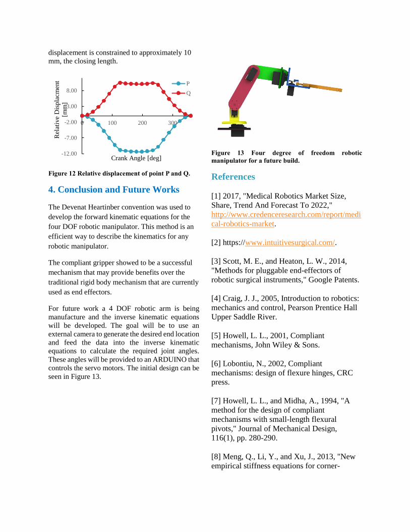
displacement is constrained to approximately 10

mm, the closing length.

Figure 12 Relative displacement of point P and Q.

4. Conclusion and Future Works

The Devenat Heartinber convention was used to

develop the forward kinematic equations for the

four DOF robotic manipulator. This method is an

efficient way to describe the kinematics for any

robotic manipulator.

The compliant gripper showed to be a successful

mechanism that may provide benefits over the

traditional rigid body mechanism that are currently

used as end effectors.

For future work a 4 DOF robotic arm is being

manufacture and the inverse kinematic equations

will be developed. The goal will be to use an

external camera to generate the desired end location

and feed the data into the inverse kinematic

equations to calculate the required joint angles.

These angles will be provided to an ARDUINO that

controls the servo motors. The initial design can be

seen in Figure 13.

Figure 13 Four degree of freedom robotic

manipulator for a future build.

References

[1] 2017, "Medical Robotics Market Size,

Share, Trend And Forecast To 2022,"

http://www.credenceresearch.com/report/medi

cal-robotics-market.

[2] https://www.intuitivesurgical.com/.

[3] Scott, M. E., and Heaton, L. W., 2014,

"Methods for pluggable end-effectors of

robotic surgical instruments," Google Patents.

[4] Craig, J. J., 2005, Introduction to robotics:

mechanics and control, Pearson Prentice Hall

Upper Saddle River.

[5] Howell, L. L., 2001, Compliant

mechanisms, John Wiley & Sons.

[6] Lobontiu, N., 2002, Compliant

mechanisms: design of flexure hinges, CRC

press.

[7] Howell, L. L., and Midha, A., 1994, "A

method for the design of compliant

mechanisms with small-length flexural

pivots," Journal of Mechanical Design,

116(1), pp. 280-290.

[8] Meng, Q., Li, Y., and Xu, J., 2013, "New

empirical stiffness equations for corner-

-12.00

-7.00

-2.00

3.00

8.00

0 100 200 300

Rel

ativ

e D

isp

lacm

ent

[mm

]

Crank Angle [deg]

P

Q

http://www.credenceresearch.com/report/medical-robotics-market

http://www.credenceresearch.com/report/medical-robotics-market

http://www.intuitivesurgical.com/

filleted flexure hinges," Mechanical Sciences,

4(2), pp. 345-356.

[9] Yong, Y. K., Lu, T.-F., and Handley, D.

C., 2008, "Review of circular flexure hinge

design equations and derivation of empirical

formulations," Precision Engineering, 32(2),

pp. 63-70.

General coordinates

8

8

78

7

7

7

6

6

6

5

5

5

4

4

4

3

3

3

2

2

2

8

8

7

7

6

6

5

5

4

4

3

3

2

2

4

3

2

y

x

y

x

y

x

y

x

y

x

y

x

y

x

r

r

r

r

r

r

r

q

q

q

q

Kinematic Constraints

0

}{

2_22

18

78

16

56

47

45

44

34

23

12

_

_

_

_

_

_

_

_

_

t

rr

rr

rr

rr

rr

rr

y

rr

rr

rr

START

II

HH

GG

FF

EE

DD

T

CC

BB

AA

DRIVER

IREV

HREV

GREV

FREV

EREV

DREV

slider

CREV

BREV

AREV

DRIVER

KINEMATIC

Kinematic Constraints

0

'

''

'

''

''

''

}{

''

''

'

2_22

1888

777888

1666

555666

444777

444555

44

333444

222333

1222

t

rsAr

sArsAr

rsAr

sArsAr

sArsAr

sArsAr

y

sArsAr

sArsAr

rsAr

START

II

HH

GG

FF

EE

DD

T

CC

BB

AA

Proceedings of

, , ,

DESIGN AND ANALYSIS OF A LOW COST PATIENT-SPECIFIC WRIST-HANDORTHOSIS

Maryam TiltonDepartment of Mechanical Engineering

Pennsylvania State UniversityUniversity Park, PA 16803Email: [email protected]

Soumyabrata Maiti∗Engineering Science and Mechanics

Pennsylvania State UniversityUniversity Park, PA 16803Email: [email protected]

ABSTRACTIn this work, we present a simple yet effective design modi-

fication of hand orthosis to help with gradual recovery of strokepatients through different stages of rehabilitation. Here, we haveused a main lever with adjustable length attached to the husk. Wehave experimentally found that as we increase the length of thelever, the mechanism does more work. We also have supportedthe result by simulating the system numerically in ADAMS.

1 IntroductionWrist-Hand Orthosis (WHO) are mainly used for maladjust-

ment correction with both mobile and immobile functionality.This is done by providing a required support for weakend mus-cle structures and increasing the function of a totally or partiallyimmobile body members [2]. Because of variety of patients andtypes of deformity, wrist-hand orthoses is often customized tomeet the unique need and anthropometric measurements of eachindividuals. Among all the causes of movement disability, strokeis considered as the primary cause, especially in developed caun-trie [1]. For many stroke patients hypertonia, spasticity, abnor-mal synergies, and extension weakness result hyperflexion of thewrist and fingers which leads to limitation of their ability to openand use their hand. This has a negative impact on their daily ac-tivity. Currently, majority of the post stroke rehabitilation takesplace in physical therapy centers [1]. In this project, our aim wasto design a wris-hand orthoses, specifically for stroke patients,that can eliminate some of the problems exist in currently avail-able deisgns. We set the following desired features as our design

∗Address all correspondence to this author.

objectives:

1. Alignment of fingers, wrist, and arm2. Providing a support for arm3. Adjustable for different stages of rehabilitation4. Can be used indepentently by patient5. Patient specific

2 Design ProceduresOur design is inspired by Eliza Wrobel’s WHO. We mod-

ified her deign by adding adjustability to main lever position.This modification allows us to evaluate the main hypothesis forthis study; which states that ”positioning the main lever furtherfrom the wrist increases the amount of work done for a sametask”. Dimensions used for the CAD model are obtained fromanthropometric measurements taken from one of the group mem-bers. After preparing the CAD model in Geomagic Design X, weproceeded with 3D printing all the parts, which were in total 77parts, using PLA filament.

3 Experimental analysis3.1 Experimental procedure

3.1.1 Objectives of the experiment Here, the ob-jective of our experiment is to find the work done by the wholemechanism under different lever lengths. In order to that, weattached one spring in between the tips of the index finger andthe thumb and let it compressed by the user. We performed theexperiment in near quasi-static condition so that the inertial ef-fects of all the links become insignificant. In that case, the energy

1 Copyright c© by ASME

Figure 1: Plot of time vs. number of oscillations.

stored inside the spring will be proportionate to the work done bythe abductor pollicis brevis muscle. Measuring this energy willhelp us to understand the effect of the adjustable lever length onthe above mentioned muscle.

Furthermore, we will study the time domain response of theangle between the distal phalange and the middle phalange (θ1)and that between palm and the proximal phalange (θ3) (see Fig.2)to obtain the insight to the muscle behaviour. Later, the ob-servations made from the experimental results will be used tonumerically model governing actuating muscle.

3.1.2 Measurement of system variables We havedone the experiment in two stages. In the first stage, we choosea random spring for the experiment. We have measured its stiff-ness by measuring its frequency of oscillation when a lump massis attached to its end. Since the the amount of the lump massis known, we have used the formulae K = ω2m to measure thestiffness. Here, K is the stiffness, ω is the frequency of oscilla-tion, and m is the mass. The natural frequency ω is calculated byfinding the amount of time taken to perform a finite number ofoscillations. Then we plot the number of oscillations against thetime and find the slope of the least square fitted line through thedata points.

At the second stage of experiment, we allow the user to grad-ually compress the spring for two cases, in the first case we setthe lever length to 57.4 mm and in the second one we changedthat to 77.4 mm. We record the movement using a 30 fps camerafor both cases and then digitized the frame to extract the anglesand the spring displacements.

Figure 2: A typical picture of the mechanism which various mea-surement variables.

Table 1: Displacement initial conditions for case I

Variable Angle (in degree)

θ1 139.896

θ2 138.043

θ3 123.490

Table 2: Displacement initial conditions for case II

Variable Angle (in degree)

θ1 132.562

θ2 125.1420

θ3 117.2640

3.2 Experimental resultsIn this section, we will discuss the experimental observa-

tions and try to construct the background for our numerical study.During the experiment, we move all the four fingers simultane-ously and focus on the movement of the index fingers. From ourobservation, we have found that the angular displacement of thethumb is negligible in compare to the other fingers. In both of ex-perimental study, initial angular displacements are listed Tables3 and 2.

In both the cases, we see the response of θ3 has a dominat-ing sinusoidal trend. Whereas the underlying trend of θ1 has afrequency which is half of the frequency if θ2. For example, the


Figure 3: Time domain response of θ1 and θ3 when the effectivelength of the main lever is 57.4 mm from the wrist. The solidline represents the fitted curve through the response of θ3

dominating frequency of θ3 for the first case is about 0.6 rad/sec(see Figs 3(a)-(b) ), whereas that fro θ1 is about 0.1 rad/sec. Thisimplies that the muscle between distant phalanges and middlephalanges acts as a nonlinear torsional spring of quadratic non-linearity. However, since our observation time frame is small, theeffect of this nonlinearity is insignificant on θ3 in this fast timescale.

Next we calculate the compressive work done on the springfor a half cycle. We have experimentally found that the stiff-ness of the spring is 125.4966 N/m. We also have calculated thedisplacements of the spring at each time step for different cases.Since the work done is define by

∫Kxdx, we employ trapezoidal

rule to find the work done for half cycle. Note that, the process

is nearly quasi-static. So we can assume that the work done bythe muscle is nearly equal to the sum of the energy stored in thespring and the energy dissipated due to various joint frictions.As the mechanism is same for both case, the energy dissipateddue to friction can be considered nearly constant in each cases.Hence, the work done on the spring is proportionate to the workdone by the muscle.

We have calculated the energy stored in the spring duringthe half cycle of the process are 0.404 and 0.426 Joule for case Iand II respectively. This result indicates that the muscle has to domore work as we increase the length of the main lever. However,the data obtained from the experiment is fairly noisy. Hence wehave employed a numerical technique to a simplified version ofthe hand mechanism with the wrist hand orthosis, which we havediscussed in details in the next section.

4 Numerical Analysis4.1 Assumptions and modelling

In previous section, we have seen that the response of θ3 hasa dominating sinusoidal feature. So if we consider the abduc-tor pollicis brevis to be a slider mechanism attached to the palmand the proximal phalanges to be the crank, the angular displace-ment response of the crank is found to be similar to that obtainedfrom the experiment. Furthermore, the constraints imposed byorthosis restricts the motion of all the fingers (except thumb) ona single plane. Hence, we can consider the real mechanism to bea two dimensional one with a slider crank mechanism represent-ing the actuating muscle. With this motivation, we now proceedto the qualitative details of our ADAMS model.

In our numerical model, we will study the two dimensionalmovements of the mechanism comprised with the index finger,the thumb, and the parts of orthosis joining them. Since, thethumb movement is insignificant in our plane of observation,thumb is considered to be the ground. We further assume thatall the links are rigid and of cuboid shape. The width and theheight of the links, depicting the hand, are taken directly fromthe subject. The values of both the parameters are set equal tothe diameter of each link. The lengths are directly measured fromthe index finger and thumb of the subject as well as the orthosismechanism. All the links are connected with revolute joints. Thejoints A, B, and C , on the index figures (see Fig. 4), also containtorsional spring (with stiffness O(102) N-mm/deg). The densityof the links, belonging to the finger, was set to 1900 kg/m3 andof those belonging to orthosis was set to 1250 kg/m3. The initialconfiguration was set in such a way that the whole mechanismsatisfied the geometrical constraints and the initial conditions ofthe angles were in close range of Case I.

A displacement profile of 2cos(1.57 ∗ t) mm was imposedon the slider to represent a constant power input to the system. Aspring of stiffness 126 N/m was placed in between the index andthumb (see Fig. 4) to study its displacement variation over time.


Figure 4: The ADAMS model used for numerical simulation.The black dots on the links represent revolute joints. The lengthof link 3 is varied only to study its effect on external work done.

As noted in the experiment, the variable θ3 is not significantlyaffect by the nonlinear stiffness of the muscle if we keep ourobservation well within the fast time scale. So we will observethe numerical response till 5 sec to avoid the effect of nonliearity.Next we discuss the observations from numerical results.

4.2 ResultsThe time domain responses of θ3 and spring displacement

are given in Figs. 5 - 6. The profiles of θ3 are very much similarto that obtained from the experiment in both the cases. Whenthe length of link 3 is 78 mm, we see that the amplitude of thedisplacement curve is about 2.5 mm. As we increase the lengthof link 3 to 112 mm, the displacement amplitude is found to bedecreased to about 0.5 mm. This has occurred because of theconsiderable fraction of input energy is diverted to the system tosatisfy the kinematic constraints as we increase the length of link3. Hence, the net available energy for the compression of thespring is reduced in later case.

This observation validates our experimental observation thatincreasing the length of link 3 will force the muscle to do morework to achieve a targeted mechanical goal.

5 ConclusionFrom the experimental results we can conclude that placing

the main lever further from the wrist, takes more power fromthe patient to perform a simple task of grabbing (using thumband index finger) comparing to when the main lever is positionedcloser to the wrist. This result justifies the adjustability featureof the design. Adjusting the position of the main lever at differ-ent stages of rehabilitation helps with gradual improvement ofmuscles. Furthermore, from the obtained results, we observedthat muscle can act as nonlinear torsional spring with quadraticnonlinearilty. These observations lead to need of future work inthis area. For the future studies, we can incorporate adjustabilityof the constraints into the design. Also, more in depth analysisof system response can help us to improve the existing math-

(a)

(b)

Figure 5: Numerically obtained time domain response of θ3 anddisplacement when the effective length of the main lever is 78mm

ematical model of the muscles. And lastly, implementation offeedback control system is suggested to mimic the hand’s natu-ral mechanism with more precision.

REFERENCES[1] Ates, S., Haarman, C. J., & Stienen, A. H. (2016). SCRIPT

passive orthosis: design of interactive hand and wristexoskeleton for rehabilitation at home after stroke. Au-tonomous Robots, 1-13.

[2] Engen, T. J. (1959). A plastic hand orthosis. Orthop. Pros.Appl. J, 13, 2. Chicago

Appendix


Tabl

e3:

My

capt

ion

Inde

xD

ista

lPha

lang

e(c

m)

Inde

xM

iddl

ePh

alan

ge(c

m)

Inde

xPr

oxim

alPh

alan

ge(c

m)

Thu

mb

Prox

imal

Phal

ange

(cm

)T

hum

bD

ista

lPha

lang

e(c

m)

L=

2.52

9L

=2.

800

L=

4.52

0L

=2.

612

L=

3.34

0D

=1.

84D

=2.

03D

=2.

19D

=2.

52D

=2.

96

Figure 6: Numerically obtained time domain response of θ3 anddisplacement when the effective length of the main lever is 112mm


ME 581: Analysis and Simulation of Rotary Engine Two—Dimensional Kinematics of a Three Flank Rotary Engine

Hugo McMenamin

Abstract

Engine design and analysis has varied throughout the history of internal combustion engines. The most popular design in modern day passenger vehicles is a reciprocating engine with pistons sliding within cylinders. One of the major detractors of this design is that the piston velocity will be zero at the top and bottom of each stroke [1]. A less popular passenger vehicle engine design is the internal combustion rotary engine which was first designed and produced by Felix Wankel with NSU [2]. This design uses the same four-stroke cycle as in reciprocating engines, however rather than a piston sliding in a cylinder, uses a rotor spinning within a housing. Because of this, rotary engines do not have any reciprocating parts including intake or exhaust valve mechanisms, and are able to have much higher power to weight ratios [3]. This report explores the two-dimensional movement of the crankshaft and rotor within the engine housing of a production rotary engine.

2. Methodology

2.1. Background

The automotive company Mazda implemented rotary engines in the RX-7 vehicles between 1978 and 2002 [4]. The engine analyzed in this report is the 13B-REW as seen in Figure 1-1, and is from the final generation of the RX-7.

Figure 1-1. Mazda 13B-REW rotary engine used in

the RX-7 FD [5]. There are three primary components of the engine, the engine housing or peritrochoid, the rotor or hypotrochoid, and the crankshaft. These are shown in Figure 1-2.

Figure 1-2. Diagram of housing, rotor, and

crankshaft [6]. The peritrochoid is defined by [1] 𝑥𝑥 = 𝑒𝑒 cos(𝛼𝛼) + 𝑅𝑅 cos�

𝛼𝛼𝑚𝑚� (1)

𝑦𝑦 = 𝑒𝑒 sin(𝛼𝛼) + 𝑅𝑅 sin �𝛼𝛼𝑚𝑚� (2)

Where x and y are the coordinates of each point on the curve, e is the eccentricity or offset of the rotor from the crankshaft, R is the generating radius or tip radius of the rotor, 𝛼𝛼 is the angle of the crankshaft, and m is the number of flanks of the rotor. As shown in Figure 1-2, eccentricity is also referred to as l, O1 is the center of the rotor, O2 is the center of the crank shaft, r2 is the radius of the crank shaft, r1 is the radius of the pitch circle within the rotor, and rroot is the distance from the center of the rotor to the center of the flank.

Given that the rotor is a three-sided closed shape, each apex or corner is 120° from the next and so the location of each can be defined by modifying (1) and (2) to be [7] 𝑥𝑥 = 𝑒𝑒 cos(𝛼𝛼) + 𝑅𝑅 cos�

𝛼𝛼𝑚𝑚

+𝑛𝑛2𝜋𝜋𝑚𝑚

� (3)

𝑦𝑦 = 𝑒𝑒 sin(𝛼𝛼) + 𝑅𝑅 sin �𝛼𝛼𝑚𝑚

+𝑛𝑛2𝜋𝜋𝑚𝑚

� (4)

Where n = 0,1,2 depending on the apex. The equations were used to validate the kinematic model of the motion of the rotor and crankshaft. 2.2. Kinematic Model Development

The first step in creating the kinematic model of the engine was to determine the two-dimensional links and joints. As shown in Figure 2-3 the housing, rotor, and crankshaft are links 1, 2, and 3.

Figure 2-3. Links 1-3 and coordinates. The apexes were then modeled as pin in slot joints accounting for 3 more links and joints as shown in Figure 2-4.

Figure 2-4. Links 4-6 and coordinates Finally, the connection between the rotor and crank shaft was modeled as an internal gear at P. The mobility of the mechanism was then analyzed using Gruebler’s equation. The pin in slots were modeled as 2 J1 joints, a revolute and prismatic, and the internal gear was modeled as a J2 joint.

Using Gruebler’s equation, this yielded a mobility of 2 meaning there is a hidden constraint. 2.3. Coordinate and constraint vectors

Based on the links and joints determined previously, the coordinate vector {𝑞𝑞} and constraint vector {𝛷𝛷} can be derived. The coordinate vector is based on the global positions and angles of each coordinate for links 2 through 6.

{𝑞𝑞}15𝑥𝑥1 =

⎩⎪⎪⎪⎨

⎪⎪⎪⎧𝑟𝑟2𝜑𝜑2𝑟𝑟3𝜑𝜑3𝑟𝑟4𝜑𝜑4𝑟𝑟5𝜑𝜑5𝑟𝑟6𝜑𝜑6⎭⎪⎪⎪⎬

⎪⎪⎪⎫

The constraint vector was generated based on the constraints for revolute joints, prismatic joints, and the internal gear join. The constraint for each revolute is defined by Haug as

{𝑟𝑟𝑖𝑖}𝑃𝑃 − �𝑟𝑟𝑗𝑗�𝑃𝑃

However here it was defined as �𝑟𝑟𝑗𝑗�

𝑃𝑃 − {𝑟𝑟𝑖𝑖}𝑃𝑃 = {02𝑥𝑥1} The constraint for each prismatic joint was defined as

�𝑦𝑦𝑖𝑖𝜑𝜑𝑖𝑖�

The constraint for the internal gear was defined by Haug as 𝛷𝛷𝑔𝑔𝑔𝑔𝑔𝑔𝑔𝑔(𝑖𝑖,𝑗𝑗) = �(𝑥𝑥𝑗𝑗𝑃𝑃 − 𝑥𝑥𝑖𝑖𝑃𝑃� 𝑠𝑠𝑠𝑠𝑛𝑛(𝜃𝜃) − �𝑦𝑦𝑗𝑗𝑃𝑃 − 𝑦𝑦𝑖𝑖𝑃𝑃� 𝑐𝑐𝑐𝑐𝑠𝑠(𝜃𝜃)}

[8] And was based on the values of xi

P, xjP, yi

P, yjP, and

𝜃𝜃 in Figure 2-5.

Figure 2-5. Internal gear set schematic [8].

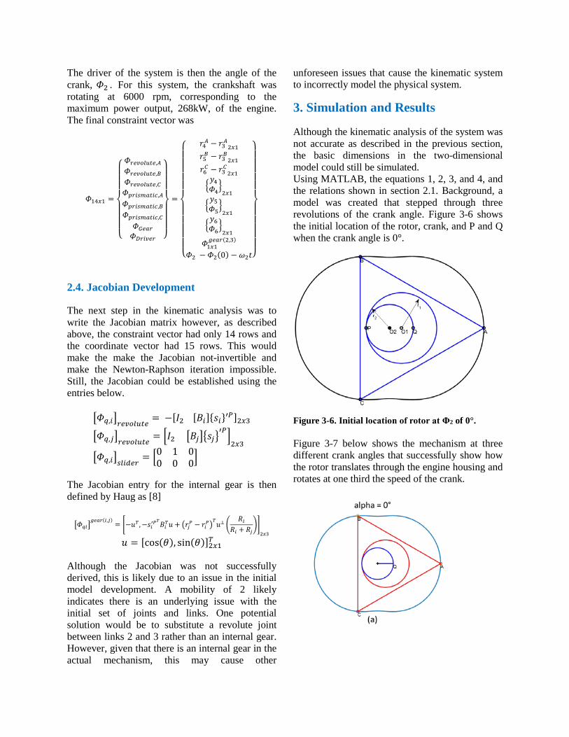
The driver of the system is then the angle of the crank, 𝛷𝛷2 . For this system, the crankshaft was rotating at 6000 rpm, corresponding to the maximum power output, 268kW, of the engine. The final constraint vector was

𝛷𝛷14𝑥𝑥1 =

⎩⎪⎪⎪⎨

⎪⎪⎪⎧𝛷𝛷𝑔𝑔𝑔𝑔𝑟𝑟𝑟𝑟𝑟𝑟𝑟𝑟𝑟𝑟𝑔𝑔,𝐴𝐴𝛷𝛷𝑔𝑔𝑔𝑔𝑟𝑟𝑟𝑟𝑟𝑟𝑟𝑟𝑟𝑟𝑔𝑔,𝐵𝐵𝛷𝛷𝑔𝑔𝑔𝑔𝑟𝑟𝑟𝑟𝑟𝑟𝑟𝑟𝑟𝑟𝑔𝑔,𝐶𝐶𝛷𝛷𝑝𝑝𝑔𝑔𝑖𝑖𝑝𝑝𝑝𝑝𝑔𝑔𝑟𝑟𝑖𝑖𝑝𝑝,𝐴𝐴𝛷𝛷𝑝𝑝𝑔𝑔𝑖𝑖𝑝𝑝𝑝𝑝𝑔𝑔𝑟𝑟𝑖𝑖𝑝𝑝,𝐵𝐵𝛷𝛷𝑝𝑝𝑔𝑔𝑖𝑖𝑝𝑝𝑝𝑝𝑔𝑔𝑟𝑟𝑖𝑖𝑝𝑝,𝐶𝐶𝛷𝛷𝐺𝐺𝑔𝑔𝑔𝑔𝑔𝑔𝛷𝛷𝐷𝐷𝑔𝑔𝑖𝑖𝑟𝑟𝑔𝑔𝑔𝑔 ⎭

⎪⎪⎪⎬

⎪⎪⎪⎫

=

⎩⎪⎪⎪⎪⎪⎨

⎪⎪⎪⎪⎪⎧ 𝑟𝑟4𝐴𝐴 − 𝑟𝑟3𝐴𝐴2𝑥𝑥1

𝑟𝑟5𝐵𝐵 − 𝑟𝑟3𝐵𝐵2𝑥𝑥1𝑟𝑟6𝐶𝐶 − 𝑟𝑟3𝐶𝐶2𝑥𝑥1�𝑦𝑦4𝛷𝛷4�2𝑥𝑥1�𝑦𝑦5𝛷𝛷5�2𝑥𝑥1�𝑦𝑦6𝛷𝛷6�2𝑥𝑥1

𝛷𝛷1𝑥𝑥1𝑔𝑔𝑔𝑔𝑔𝑔𝑔𝑔(2,3)

𝛷𝛷2 − 𝛷𝛷2(0) − 𝜔𝜔2𝑡𝑡⎭⎪⎪⎪⎪⎪⎬

⎪⎪⎪⎪⎪⎫

2.4. Jacobian Development

The next step in the kinematic analysis was to write the Jacobian matrix however, as described above, the constraint vector had only 14 rows and the coordinate vector had 15 rows. This would make the make the Jacobian not-invertible and make the Newton-Raphson iteration impossible. Still, the Jacobian could be established using the entries below.

�𝛷𝛷𝑞𝑞,𝑖𝑖�𝑔𝑔𝑔𝑔𝑟𝑟𝑟𝑟𝑟𝑟𝑟𝑟𝑟𝑟𝑔𝑔 = −[𝐼𝐼2 [𝐵𝐵𝑖𝑖]{𝑠𝑠𝑖𝑖}′𝑃𝑃]2𝑥𝑥3

�𝛷𝛷𝑞𝑞,𝑗𝑗�𝑔𝑔𝑔𝑔𝑟𝑟𝑟𝑟𝑟𝑟𝑟𝑟𝑟𝑟𝑔𝑔 = �𝐼𝐼2 �𝐵𝐵𝑗𝑗��𝑠𝑠𝑗𝑗�′𝑃𝑃�

2𝑥𝑥3

�𝛷𝛷𝑞𝑞,𝑖𝑖�𝑝𝑝𝑟𝑟𝑖𝑖𝑠𝑠𝑔𝑔𝑔𝑔 = �0 1 00 0 0�

The Jacobian entry for the internal gear is then defined by Haug as [8]

�𝛷𝛷𝑞𝑞𝑖𝑖�

𝑔𝑔𝑔𝑔𝑔𝑔𝑔𝑔(𝑖𝑖,𝑗𝑗)= �−𝑢𝑢𝑇𝑇,−𝑠𝑠𝑖𝑖′𝑃𝑃

𝑇𝑇𝐵𝐵𝑖𝑖𝑇𝑇𝑢𝑢 + �𝑟𝑟𝑗𝑗𝑃𝑃 − 𝑟𝑟𝑖𝑖𝑃𝑃�𝑇𝑇𝑢𝑢⊥ �

𝑅𝑅𝑖𝑖𝑅𝑅𝑖𝑖 + 𝑅𝑅𝑗𝑗

��2𝑥𝑥3

𝑢𝑢 = [cos(𝜃𝜃), sin(𝜃𝜃)]2𝑥𝑥1𝑇𝑇 Although the Jacobian was not successfully derived, this is likely due to an issue in the initial model development. A mobility of 2 likely indicates there is an underlying issue with the initial set of joints and links. One potential solution would be to substitute a revolute joint between links 2 and 3 rather than an internal gear. However, given that there is an internal gear in the actual mechanism, this may cause other

unforeseen issues that cause the kinematic system to incorrectly model the physical system.

3. Simulation and Results

Although the kinematic analysis of the system was not accurate as described in the previous section, the basic dimensions in the two-dimensional model could still be simulated. Using MATLAB, the equations 1, 2, 3, and 4, and the relations shown in section 2.1. Background, a model was created that stepped through three revolutions of the crank angle. Figure 3-6 shows the initial location of the rotor, crank, and P and Q when the crank angle is 0°.

Figure 3-6. Initial location of rotor at Φ2 of 0°. Figure 3-7 below shows the mechanism at three different crank angles that successfully show how the rotor translates through the engine housing and rotates at one third the speed of the crank.

Figure 3-7. Rotor and crank position simulation at varying crank angles.

4. Conclusion

Although the Newton-Raphson simulation of the kinematics of the rotary engine were not successful, the two-dimensional simulation of the system based on the governing geometrical equations, proved the underlying logic. The results of the simulation showed the actual motion of the rotary engine. The rotor rotated at one third the speed of the crankshaft, which follows based on the operation of a rotary engine [3]. In future work, the initial coordinates and constraints need to be revisited to determine the underlying issue. Once adjusted, the Newton-Raphson solution can be completed and compared with the two-dimensional simulation results.

References

[1] K. Yamamoto, Rotary Engine, Tokyo: Tokyo Kogyo Co., Ltd., 1971.

[2] Encyclopedia Britannica Inc., "Felix Wankel," Encyclopedia Britannica Inc., 2009. [Online]. Available: https://www.britannica.com/biography/Felix-Wankel.

[3] K. Yamamoto, Rotary Engines, Tokyo: Tokyo Kogyo Co. Ltd., 1981.

[4] Mazda Motor Corporation, "History(1920～1979)," Mazda Motor Corporation, [Online]. Available: http://www.mazda.com/en/about/profile/history/1920-1979/.

[5] N. Stecher, "Mazda’s Confusing Plan to Resurrect the Famously Dirty Rotary Engine," 2015. [Online]. Available: https://www.wired.com/2015/12/mazdas-confusing-plan-to-resurrect-the-famously-dirty-rotary-engine/#slide-6.

[6] S. W. Rose and D. C. H. Yang, "The Deviation Function," Journal of Mechanical Design, vol. 136, 2014.

[7] K. C. Weston, Energy Conversion, The University of Tulsa, 1999.

[8] E. J. Haug, Computer Aided Kinematics and Dynamics of Mechanical Systems, 1989: Prentice Hall College Div.

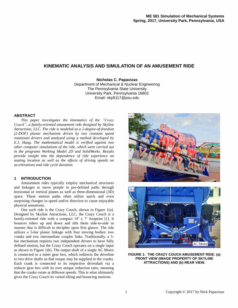
1 Copyright © 2017 by Nick Papavizas

ME 581 Simulation of Mechanical Systems Spring, 2017, University Park, Pennsylvania, USA

KINEMATIC ANALYSIS AND SIMULATION OF AN AMUSEMENT RIDE

Nicholas C. Papavizas Department of Mechanical & Nuclear Engineering

The Pennsylvania State University University Park, Pennsylvania 16802

Email: [email protected]

ABSTRACT This paper investigates the kinematics of the “Crazy

Couch”, a family-oriented amusement ride designed by Skyline

Attractions, LLC. The ride is modeled as a 2-degree-of-freedom

(2-DOF) planar mechanism driven by two constant speed

rotational drivers and analyzed using a method developed by

E.J. Haug. The mathematical model is verified against two

other computer simulations of the ride, which were carried out

in the programs Working Model 2D and SolidWorks. Results

provide insight into the dependence of ride experience on

seating location as well as the effects of driving speeds on

accelerations and ride cycle duration.

1 INTRODUCTION Amusement rides typically employ mechanical structures

and linkages to move people in pre-defined paths through

horizontal or vertical planes as well as three-dimensional (3D)

space. These motion paths often utilize quick and even

surprising changes in speed and/or direction to cause enjoyable

physical sensations.

One such ride is the Crazy Couch, shown in Figure 1(a).

Designed by Skyline Attractions, LLC, the Crazy Couch is a

family-oriented ride with a compact 18’ x 7’ footprint [1]. It

bounces riders up and down and tilts them side-to-side in

manner that is difficult to decipher upon first glance. The ride

utilizes a 5-bar planar linkage with four moving bodies: two

cranks and two intermediate coupler links. Traditionally, a 5-

bar mechanism requires two independent drivers to have fully

defined motion, but the Crazy Couch operates on a single input

as shown in Figure 1(b). The output shaft of a single AC Motor

is connected to a miter gear box, which redirects the driveline

to two drive shafts so that torque may be supplied to the cranks.

Each crank is connected to its respective driveshaft via a

reducer gear box with its own unique reduction ratio, meaning

that the cranks rotate at different speeds. This is what ultimately

gives the Crazy Couch its varied tilting and bouncing motions.

FIGURE 1: THE CRAZY COUCH AMUSEMENT RIDE: (a) FRONT VIEW (IMAGE PROPERTY OF SKYLINE

ATTRACTIONS) AND (b) REAR VIEW.

(a)

(b)

AC Motor


(1)

(2)

(3)

This paper explores the motions and sensations one may

experience while riding the Crazy Couch via theoretical

kinematic analysis and computer simulation. Kinematic

equations of motion for the fundamental mechanism of the

Crazy Couch are derived using the analysis methods developed

by E.J. Haug for constrained multibody systems [2]. These

equations are programmed into MATLAB [3] and the results

are compared with those obtained from computer simulations

of the Crazy Couch carried out using two different simulation

programs: Working Model 2D [4] and SolidWorks + Motion

Analysis [5]. Finally, a sensitivity study is performed in which

the gear ratios of the reduction gear boxes are varied in order

investigate effects on ride aspects such as maximum

acceleration magnitudes at different locations on the

mechanism and ride cycle duration.

2 METHODOLOGY

2.1 Simple Model and Mobility

The fundamental mechanism of the ride is a 5-bar planar

mechanical linkage as depicted in the skeletal diagram of

Figure 2, which views the ride from the front as in Figure 1(a).

The mechanism exists in a vertical plane with X taken to be the

horizontal direction and Y taken to be the vertical. The

mechanism comprises four moving bodies: a first crank (link

2), the seat span (link 3), a slider block or trolley (link 4), and a

second crank (link 5). Ground is traditionally labeled link 1.

Points A, B C, and D represent revolute joints connecting link 2

to ground, link 2 to link 3, link 4 to link 5, and link 5 to ground,

respectively. On the Crazy Couch the slider trolley sits in a

linear bearing on the underside of the seat span, so the interface

between links 4 and 5 in Figure 2 is a translational/prismatic

joint that allows the seat span to slide over the second crank.

FIGURE 2: KINEMATIC SKELETAL DIAGRAM OF THE 5-BAR MECHANISM OF THE CRAZY COUCH.

It should be noted that the translational axis of the

prismatic joint is offset from but always remains parallel to the

line connecting joints B and C. Kinematically speaking,

whether this translational axis is inline or offset makes no

difference. It does make a difference, however, for dynamics

where the offset distance has a significant impact on the forces

acting on the prismatic joint and pin joint at C. This offset

distance is kept relatively small compared to the overall scale

of the ride. The mobility of this mechanism can be verified

using the Kutzbach equation for two-dimensional mobility [6]:

M = 3(nL – 1) – 2(nJ1) – 1(nJ2)

where nL is the number of links (including ground), nJ1 is the

number of full joints, and nJ2 is the number of half joints. An

unconstrained body in planar space has three degrees-of-

freedom (DOF). Full joints, such as revolute and prismatic

joints, allow movement in one direction, thereby restricting two

DOF. Half joints allow movement in two directions and restrict

only one. In this case nL = 5, nJ1 = 5, and nJ2 = 0, so the

mobility of the Crazy Couch is M = 2-DOF. As expected, a 5-

bar mechanism requires two drivers in order to have fully

defined motion. In this case, the two required inputs are the

constant angular velocities ω2 and ω5 as shown in Figure 2.

2.2 Kinematic Equations

In accordance with Haug’s method [2], the motion of the

mechanism can be described by a set of generalized coordinates

that represent the global positions and attitudes of the moving

links. The generalized coordinates for this mechanism are

defined as follows:

{2,3,4,5}iyxr}{qT

iii

T

iT

ii

where xi and yi represent the global horizontal and vertical

positions, respectively, and ϕi represents the attitude of the ith

link. The generalized coordinates Eq. (2) can then be

concatenated into a single generalized coordinate column

vector Eq. (3):

TT5

T4

T3

T2 }{q}{q}{q}{q{q}

In total, the mechanism has twelve generalized coordinates.

Figure 3 shows local body-fixed coordinate frames that are

attached to each of the links. These local coordinate frames

allow the positions of various points on the links to be

described in terms of invariant distances; they stay the same for

all time, no matter the position or orientation of the body. The

orientations angles ϕi of the local frames with respect to the

global directions are measured the counter-clockwise (CCW)

from the global X axis to the local x'i axes. For convenience

and simplicity, the origins of the local coordinate frames are

placed at the centers of revolute joints.

In Figure 3(b), the points R4 and S4 on link 4 are collinear

with the translational path of link 4 along the length of link 3.

In Figure 3(d), the points P3 and Q4 on link 3 are also collinear

with the translational path of link 4 along the length of link 3.

These points are necessary for writing vectors and constraints

that enforce the prismatic joint, as will be described below.

The local positions of all the points on the links in Figure 3

are necessary pieces of information about the geometry of the

mechanism to be able to perform kinematic analysis. Specific

values of these geometries will not be given in this paper per a

non-disclosure agreement between the author and Skyline

Attractions, LLC.

A

B

C D 1

2

3

5

4 ω2

ω5

Y

X


(4)

(5)

(6)

The mechanism is 2-DOF and has twelve generalized

coordinates, so, per Haug [2], a total of twelve constraints are

needed to enforce the constrained motion of the mechanism.

Specifically, ten kinematic constraints are needed to limit the

mobility of the mechanism to 2-DOF, and then two driving

constraints are needed to fully define its motion. Algebraic

position and driving constraints presented in Haug [2] are

written in Eq. (4):

1x12

55_START5

22_START2

34

TT

3

4

TT

3

D

1

D

5

C

4

C

5

B

2

B

3

A

1

A

2

DRIVER_D

DRIVER_A

PIN_SLOT

PARALLEL

REV_D

REV_C

REV_B

REV_A

0

tω

tω

dRa

aRa

rr

rr

rr

rr

Φ

Φ

Φ

Φ

Φ

Φ

Φ

Φ

Φ

Rows one through eight of the 12 x 1 constraint vector {Φ}

are revolute constraints that enforce the pin joints at Points A,

B, C and D. The expressions of the form {rj}P – {ri}

P = {02x1}

state that global position of point “P” on two separate bodies

“j” and “i” must be coincident at all times. The next two rows

enforce the prismatic joint between link 3 (seat span) and link 4

(slider trolley) by stating that the vectors {a4} and {d34} must

always remain parallel to the vector {a3} (see Figure 3). The

term [R] is a 2 x 2, 90-degree CCW rotator matrix. The last two

rows are relative angle driver constraints that apply constant

speed rotation to the cranks, where link 2 (first crank) is driven

from Point A at constant angular velocity ω2 and link 5 (second

crank) is driven from Point D at constant angular velocity ω5,

CCW is taken to be the positive direction.

These generalized coordinates {q} and constraints {Φ} are

then used to determine the position of each link in the global

reference frame. Due to the nonlinearity of position equations, a

Newton-Raphson algorithm Eq. (5) is employed to solve for

updated values of the generalized coordinates at a new time

step k+1 based on initial guesses of {q} taken at the current

time step k:

k1

kqkkk1k qqqq

The term [Φq] is a matrix of partial derivatives of the

constraints taken with respect to the generalized coordinates

known as the Jacobian matrix, as shown in Eq. (6):

nq,,2,1j,nc,,2,1i,

q j

iq

where nc is the number of constraints and nq is the number of

generalized coordinates. For the Crazy Couch, the Jacobian is a

12 x 12 matrix. The Jacobians terms for planar revolute and

prismatic joints and the relative angle drivers can be found in

Chapter 3 of [2].

To start the Newton-Raphson algorithm Eq. (5), initial

global positions and orientations of the links are estimated from

the initial pose of the Crazy Couch shown in Figure 4, where

the seat span is horizontal with respect to the ground and at its

FIGURE 3: ILLUSTRATION OF LOCAL COORDINATE FRAME SET UP AND ASSOCIATED LINK

PARAMETERS FOR (a) LINK 2, (b) LINK 4, (c) LINK 5, AND (d) LINK 3.

x'2

y'2

B2

A2

x'5

y'5

C5

D5

C4 x'

4

y'4

R4

S4

B3 x'

3

y'3

Q3

P3

𝑎4

𝑎3

𝑑34

Φ2

Φ5 Φ4

Φ3

(a) (b) (c)

(d)


(7)

(8)

(9)

(10a)

(10b)

(10c)

(10d)

(11a)

(11b)

(11c)

(12)

(11d)

lowest position relative to Points A and D. It is in this position

that the ride starts and ends and in which riders load onto and

disembark from the ride.

FIGURE 4: INITIAL POSE OF THE MECHANISM.

With the position solution obtained from Eq. (5), velocity

and acceleration solutions are straightforward to obtain

thereafter and can be calculated during each time step. The

velocity solution presented by Haug [2] is given by Eq. (7):

tq forq

where q are the generalized velocities, {ν} is the velocity

right-hand side (RHS) and {Φt} is the first partial of the

constraint vector with respect to time. For scleronomic

constraints that are independent of time, such as mechanical

joints, the velocity RHS is zero. The acceleration solution

presented by Haug [2] is given by Eq. (8):

tttqqqq q2qqforq

where q are the generalized accelerations and {γ} is the

acceleration RHS, which includes second partials derivatives of

the constraint vector with respect to the generalized coordinates

and time. For constrained multibody systems like the Crazy

Couch with only scleronomic constraints, all second partials of

the kinematic constraints are zero and Eq. (8) reduces to

qqforqqqq

The velocity RHS’s and acceleration RHS’s presented by Haug

[2] for the joints and drivers employed in the Crazy Couch are

shown in Eq. (10) and Eq. (11):

1x2REV 0

0PARALLEL

0PIN_SLOT

DRIVER

Pii

2i

Pjj

2jREV 'sA'sA

0PARALLEL

REVij2

iT

ijiT

iPIN_SLOT dRd2a

0DRIVER

The terms [Aj] and [Ai] are orthonormal rotation matrices that

describe the attitudes of generic bodies “j” and “i”, which are

used to convert information described in local coordinates to

global coordinates and vice versa.

2.3 MATLAB Algorithm

Position, velocity, and acceleration analyses are carried out

in MATLAB over one full cycle of the mechanism in mid-

operation (neglecting start up and slow down). Since the cranks

link 2 and link 5 rotate at different speeds, a full cycle can be

defined as the time or the number of rotations of each crank it

takes for the mechanism to return to its starting pose as shown

in Figure 4. Nominally, the Crazy Couch operates so that the

cranks rotate at a relative speed ratio of 5:4, meaning that for

every five revolutions of link 2 there are four revolutions of

link 5 in a single cycle. Then the cycle duration, denoted herein

as tcycle, can be calculated using Eq. (12):

cycleper revscrank ofnumber 2

tcrank

cycle

where either of the crank speeds (in radians per second) and

corresponding number of revolutions per cycle can be used.

An explicit time loop is utilized to perform the position,

velocity, and acceleration analyses described by Eq. (2) through

Eq. (11) at each time step starting from t = 0. A number of time

steps per second, n, is defined and the time step size, Δt, is

calculated as 1/n. Therefore, the total number of time steps is

tcycle/Δt (rounded up to the next whole number if necessary).

At each time step, the global orientations of the cranks, ϕ2

and ϕ5, are updated based on the current time, ω2 and ω5.

Global positions and orientations from the last time step are

used as initial estimates for the positions at the current time

step. The numerical convergence criteria for the Newton-

Raphson algorithm Eq. (5) is when the constraints become

sufficiently close to zero. In this case, Eq. (5) is iterated until

max(abs({Φ})) < ε, where ε is an assembly tolerance. An

assembly tolerance of ε = 10-5

cm is chosen given the scale of

the ride. The data from the kinematic analyses are stored and

the time step is updated.

2.4 Comparison Models

In order to verify the accuracy of the mathematical model

developed in Sections 2.2 and 2.3, two other models of the

Crazy Couch were created using the commercial simulation

packages Working Model 2D [4] and SolidWorks [5] with

Motion Analysis add-on. Figure 5 shows the model created in

Working Model and Figure 6 shows the model created in

SolidWorks.

Working Model enforces constraints between rigid bodies

in manner much like the method presented by Haug [2].

However, instead of performing exact kinematics when

carrying out simulations, Working Model utilizes forward time

integration in which dynamic forces are used to predict

resulting motion. Forward time integration can result in


solutions “blowing up” if a mechanism is not well behaved or if

the time step size is not chosen sufficiently small. Therefore, a

time step of Δt = 0.002 seconds, or n = 500 steps per second,

was chosen for all three of the simulations (MATLAB, Working

Model, SolidWorks) for the verification step.

The basic implementation of SolidWorks motion analysis

also performs exact kinematics when a kinematic driver such as

a constant speed rotational driver is chosen.

Simulations were carried out in all three programs using

identical geometries, initial positions, driving speeds, and time

steps as mentioned previously.

3 RESULTS

3.1 Model Verification

For the simulations, ω2 and ω5 were set to the nominal

operating speeds of 21.75 RPM and 17.4 RPM, respectively,

FIGURE 7: ROTATIONAL KINEMATICS OF THE SEAT SPAN

OVER A FULL CYCLE – HAUG’S METHOD (SOLID) COMPARED WITH WORKING MODEL 2D (DASHED).

which are based on the standard RPM of the Crazy Couch’s AC

motor and reduction ratios, thus yielding the appropriate 5:4

relative speed ratio. Both ω2 and ω5 were set clockwise (CW).

The rotational kinematics of the seat span (link 3) were chosen

as the metric for comparison because this link goes through the

most complicated motion. These rotational kinematic metrics

includes the attitude angle of the seat span ϕ3 and its first and

second derivatives, ϕ̇3 and ϕ̈3.

Data from the Working Model and SolidWorks simulations

were collected and plotted against the corresponding solution

obtained from the MATLAB implementation of the Haug

model. Data from Working Model is compared with the

MATLAB solution in Figure 7. Data from SolidWorks is

compared with the MATLAB solution in Figure 8. There is

clear agreement between the solutions, with the dashed lines

(Working Model) and dotted lines (SolidWorks) following the

solid lines (MATLAB) without any appreciable difference.

Also, the results indicate motion that is consistent with the

FIGURE 8: ROTATIONAL KINEMATICS OF THE SEAT SPAN

OVER A FULL CYCLE – HAUG’S METHOD (SOLID) COMPARED WITH SOLIDWORKS (DOTTED).

FIGURE 5: WORKING MODEL 2D CRAZY COUCH MODEL

FIGURE 6: SOLIDWORKS CRAZY COUCH MODEL


FIGURE 9: ERROR BETWEEN HAUG’S METHOD AND WORKING MODEL 2D SEAT SPAN (LINK 3) ROTATIONAL

KINEMATICS SOLUTIONS OVER A FULL CYCLE.

real mechanism. There are five peaks corresponding to the five

revolutions of link 2 in one cycle, with the largest rotations,

angular velocities, and angular velocities occurring when the

two cranks are out of phase and the smallest occurring when

cranks become in phase.

The errors between these solutions are plotted in Figures 9

and 10. The overall error between the Working Model

simulation and the MATLAB solution is greater than the error

between the SolidWorks simulation and the MATLAB solution.

This can be primarily attributed to reasons mentioned in

Section 2.4, where Working Model performs forward time

integration as opposed to exact kinematics.

As Figure 9 shows, one effect of numerical integration is

that solution accuracy decreases every time a derivative is taken

and when the function being integrated changes rapidly over

time. In Figure 7, the most rapid change in acceleration occurs

around the zero crossing after the third peak at around 7.5

seconds into the cycle. Observation of Figure 9 shows that this

is also when the largest error between the acceleration solutions

occurs. Furthermore, one other possibility for the relatively

large error—order of 10-4

—is because the translational path of

link 4 along link 3 was made collinear with the line connecting

the revolute joints at Point C in the Working Model simulation

(compare Figures 2 and 5). As mentioned previously in Section

2.1, the offset of the prismatic joint (or lack thereof) makes a

difference in dynamic analysis. It is expected that recreating the

Working Model simulation with the exact offset prismatic joint

geometry as the MATLAB and SolidWorks models would

significantly decrease the relative solution error. However,

errors on the order of 10-4

is still very small given the scale of

the mechanism and the solutions can be considered near-exact

matches for practical purposes.

FIGURE 10: ERROR BETWEEN HAUG’S METHOD AND SOLIDWORKS SEAT SPAN (LINK 3) ROTATIONAL KINEMATICS SOLUTIONS OVER A FULL CYCLE.

The error between the SolidWorks and MATLAB position,

velocity, and acceleration solutions, shown in Figure 10, jumps

sporadically around values on the order of 10-10

, which is most

likely only that large because of rounding differences incurred

when entering numerical geometry data into the two programs.

Because the error between the SolidWorks and MATLAB

solutions is so small, it can be inferred that plotting the error

between the Working Model and SolidWorks simulations would

yield a similar characteristic to the one shown in Figure 9.

These results prove that the mathematical model developed

following Haug [2] accurately predicts the theoretical motions

of the moving bodies that comprise the Crazy Couch.

3.2 Rider Experience: Motion Profiles and Accelerations

The mathematical model can be used to learn pertinent

information about the kinematics of the amusement ride. First

and foremost, it should be noted that the kinematic analysis

methods of Haug [2] provide a straightforward link to both

inverse and forward dynamics. In this case, the Crazy Couch is

treated as a kinematically driven problem; finding the Cartesian

and rotational accelerations of the centers of the gravity of all

the moving links, combined with knowing each of their mass

and inertia properties, would allow an engineer to perform

inverse dynamics in order to find joint reaction forces and the

torques required to drive the two cranks. Dynamic analysis was

not a focus of this paper, but it is certainly a prospect for future

work.

However, another critical element in the design of an

amusement ride is the experience of the riders: to what types of

motions and accelerations will the riders be subjected, and are

those motions within safe limits? Figure 11 shows a front view

of the Crazy Couch. Points of interest are marked by red circles


and local coordinate systems indicating their global positions in

the XY plane defined in Figure 2. These points represent the

approximate locations of a rider (chest to head level, depending

on height) when they sit in the left end seat (Point L), either of

the two middle seats (Point M), or the right end seat (Point R)

on the seat span.

FIGURE 11: THREE RIDER LOCATIONS ON THE SEAT SPAN CHOSEN FOR ANALYSIS: LEFT END SEAT (L),

MIDDLE SEATS (M), AND RIGHT END SEATS (R).

The motion profiles experienced by riders sitting in these seats

can be obtained by plotting the global positions of Points L, M,

and R over a full cycle of the mechanism. This is shown in

Figure 12, where the black circles indicate the coincident

starting and ending positions of Points L, M, and R. Point L

follows the blue path (left), Point M follows the red path

(middle), and Point R follows the yellow path (right). The CW

circular paths followed by the cranks around their ground

connection points, A and D, are plotted for reference.

FIGURE 12: MOTION PROFILES OF POINTS L, M, AND R.

As one moves from left to right on the seat span (facing the ride

from the front as in Figure 11), the motion experienced varies.

In the left end seat (Point L), the rider will essentially move in a

clockwise circular path that follows first crank (link 2) and gets

stretched and warped due to the back-and-forth tilting of the

seat span. Looking at the middle seats (Point M), the overall

motion envelope decreases, but the rider will start to experience

direction changes that result from the sliding of the seat span

over the second crank (link 5) as the two cranks rotate at

different speeds. Moving all the way to the right end seat (Point

R), the range of motion increases, somewhat combining and

intensifying the vertical stretch seen in motion profile of Point

L and the direction changes in the motion profile of Point M.

The question then becomes, what does this mean for sensations

felt by the riders? In other words, what accelerations are they

subjected to?

ASTM F 2291 on the “Standard Practice for Design of

Amusement Rides and Devices” [6] establishes strict

limitations on allowable accelerations that patrons can be

subjected to in a given plane of motion relative to anatomical

directions of the human body. Taking definitions from [6], the

Crazy Couch moves riders in the human body’s coronal (YZ)

plane, with the left and right lateral directions in the Y the

cranial and caudal directions in the Z. Figure 13 shows a

standard graphical tool from [6] that is used to visualize

allowable accelerations in this plane (accelerations in g’s).

FIGURE 13: ALLOWABLE COMBINED MAGNITUDES OF Y (HORIZONTAL) AND Z (VERTICAL) ACCELERATIONS [6].

Any component of total acceleration experience by riders of the

Crazy Couch need to meet individual axis requirements, and


total combined acceleration magnitude must fall inside the so-

called “acceleration egg”.

Because the Crazy Couch is a “family-oriented” ride—not

a high-speed thrill ride like a roller coaster, a 300+ ft. drop

tower, or a giant pendulum ride—it is expected that the

horizontal and vertical accelerations will be relatively small,

but noticeable enough to cause pleasant sensations that

ultimately make the ride fun for amusement park patrons. These

accelerations are sometimes referred to colloquially as “g-

forces” when the quantities are normalized by the gravitational

acceleration constant 9.81 m/s2 (32.2 ft/s

2).

Horizontal accelerations felt by riders, as shown in Figure

14, are relatively mild on the Crazy Couch, with a peak value

of about 0.4 g’s to the right occurring at only one instant in the

right end seat (Point R). Accelerations seldom exceed 0.3 g’s in

either direction for any of the points of interest. There is also

little variation from left to right on the seat span; the

acceleration profiles of all the points follow roughly sinusoidal

paths with similar periodicities and amplitudes. What this

translates to in terms of physical sensations is a gentle left-to-

right rocking/swaying felt in all the seats, which is unlikely to

cause any discomfort to riders, perhaps aside from mild nausea

in those who are prone to motion sickness.

FIGURE 14: HORIZONTAL ACCELERATIONS EXPERIENCED BY RIDERS.

Vertical accelerations felt by riders is a different story, as can be

seen in Figure 15. Where one sits on the seat span could make a

difference in the intensity of “heaviness” and “losing one’s

stomach” sensations felt. For example, a rider sitting in the left

end seat will experience a near-harmonic variation in the

perception of their weight similar to what one may feel while

swinging on a swing set, with peaks regularly reaching 0.2 to

FIGURE 15: VERTICAL ACCELERATIONS EXPERIENCED

BY RIDERS.

0.3 g’s above and below 1 g. This is consistent with the oblong

oval motion path of Point L in Figure 12.

Riders sitting in the middle seat of the Crazy Couch (Point

M) will feel weaker vertical accelerations overall (magnitudes

less than 0.2 g above and below 1 g), but the variations from

positive to negative may feel less “planned” and more

“random”, as evidenced from the clear deviation from a simple

sinusoidal profile. This is consistent with the smaller motion

envelope and direction changes of Point M in Figure 12.

As the motion profile of Point R seems to combine and

intensify those of Points L and M, so goes the acceleration. A

rider sitting in the right end seat will encounter the most drastic

bouncing, with two moments of noticeable heaviness where

accelerations peak at just below 1.4 g’s and three moments of

noticeable lightness with acceleration dipping below 0.6 g’s at

one instant around 7.5 seconds into the cycle.

It is interesting and intuitive to note that motion and

acceleration profiles of seats closer to the first crank (link 2)

have five distinctive peaks within one cycle, whereas those of

the seats closer to the second crank (link 5) seem to have four

distinctive peaks within one cycle. This is a direct effect of the

5:4 speed ratio of link 2 to link 5. It also clear from Figures 14

and 15 that accelerations experienced by riders fall well within

the margins imposed by ASTM 2291 F [6].

Although excitement on amusement rides is entirely

subjective, and while the Crazy Couch is a milder ride in

general, someone looking for the most intense forces and

“quirky” bouncing motions may wish to sit in the right end

seat, which sits to the outside of the sliding joint. Perhaps the

greater takeaway is that each rider will have a slightly different

experience from the riders he or she sits next to. Furthermore,

Eyes right

Eyes left

Eyes down

Eyes up


this means that one can ride the Crazy Couch multiple times

and get a different experience each time.

3.3 Model Visualization

A short program was written in MATLAB to animate a

visual representation of the Crazy Couch 5-bar mechanism as

the ride moves through one full cycle. Real-time visualization

of a mechanism can be a helpful design tool. The built-in

function ‘VideoWriter’ is also used to create a video file of the

animation that can be played back. At each time step, the

positions of reference points and outlines of the links are

plotted on the same figure, written as a single frame into the

video file, and then updated at each subsequent time step. This

program follows the basic structure shown below. A sample

frame of the output is shown in Figure 16, which also includes

real-time tracing of the rotational kinematics of the seat span.

1 % Set up video file

2

3 v = VideoWriter('cc.avi');

4 v.FrameRate = fr; % set frame rate

5 open(v);

6 7 % sequence through positions

8

9 for i = 1 : length(t_cycle)

10

11 % plot all points on links

12

13 % write images to video file

14 M = getframe(gcf);

15 writeVideo(v,M);

16

17 end

18

19 close(v);

FIGURE 16: SCREENSHOT OF A MATLAB ANIMATION OF

THE CRAZY COUCH AND SEAT SPAN ROTATIONAL KINEMATICS.

3.4 Sensitivity Study

The Crazy Couch is currently manufactured under one set

of specifications in terms of link geometries, input motor speed,

and relative crank speeds. While modifying the design from its

current form may or may not be economical, an obvious

question stemming from a standpoint of pure curiosity is, what

types of different motions can be obtained by changing certain

parameters of the mechanism? In this paper, the parameters

chosen for variation are the speeds of the two cranks ω2 and ω5

and, therefore, the ratio between them, ω2 / ω5. This is achieved

by assuming a constant operating speed of the input AC motor

and simply adjusting the reduction ratios of the reducer gear

boxes that connect to the cranks. The author realizes that

adjusting gear ratios in the mechanism can also change torque

and power requirements, but it certainly the simplest

modification from a design standpoint and is likely to be less

costly than changing entire geometries of the moving links,

which would require full redesigns of numerous parts of the

mechanism and the supporting structure.

Reduction ratios for each of the two reduction gear boxes

are determined based on the capabilities of the manufacturer of

the current reducer model employed on the Crazy Couch.

Furthermore, reduction ratios are also chosen to ensure that the

ratio of the crank speeds ω2 / ω5 is always a rational number,

i.e., a fraction of two integers. This prevents the possibility of

impossibly long ride cycle durations.

To show the effects of this parameter variation in a

succinct way, the maximum acceleration magnitudes of

different points on the links that are achieved during one cycle

of the mechanism are plotted as functions of ω2 and ω5. From

this it is possible to see whether accelerations at rider locations

such as Points L, M, and R remain within the allowable ranges

set forth by ASTM F 2291 [6]. Analyzing the acceleration

magnitudes at the joints (Points A, B, C, D, and the prismatic

joint) would additionally help determine whether the crank

speeds are appropriately safe for a given construction of the

mechanism—dynamic effects on the mechanism itself should

also be considered.

The resulting ride cycle durations tcycle are also plotted as

functions of ω2 and ω5 in order to determine whether the

selected gear ratios would yield a practical ride duration. If the

cycle is too short, then the ride becomes repetitious. If the cycle

is too long, then the ride could be hampered down by low

ridership capacity.

Sample results taken at Point R (right end seat) are

presented in Figure 17 for an input speed of 870 RPM.

Maximum acceleration magnitudes are plotted in Figure 17(a)

and the corresponding ride cycle durations are plotted in Figure

17(b). The reduction ratio applied to link 2, which produces the

output speed ω2, is the abscissa and the resulting acceleration

and tcycle are the ordinates. Different curves are produced by

varying the value of the reduction ratio applied to link 5, which

produces the output speed ω5. Circled in red is the nominal

operating point of the Crazy Couch, where reduction ratios of

40:1 to link 2 and 50:1 to link 5 result in ω2 = 21.75 RPM and

ω5 = 17.4 RPM, respectively. With these parameters, the


maximum acceleration magnitude felt by a rider in the right end

seat is just under 1.5 g’s and the ride cycle duration is just

under 14 seconds.

FIGURE 17: DEPENDENCE OF (a) MAXIMUM ACCELERATION MAGNITUDES AT POINT R AND (b) RIDE

CYCLE DURATION ON RELATIVE CRANK SPEEDS.

It can be seen that under the right combinations of gear

ratios, the maximum accelerations and ride cycle durations can

be increased or decreased dramatically. As expected, choosing

lower gear ratios for both reducers results in much faster crank

speeds, which then increase the accelerations felt by the riders.

Ride cycle duration shoots up when the gear ratios are slightly

mismatched and drops significantly when the reduction ratios

are integer multiples of one another.

CONCLUSIONS Amusement rides often incorporate various translating and

rotating parts connected through mechanical joints and linkages

in order to produce exciting motions for park patrons. As such ,

they are constrained multibody systems. The kinematic analysis

method of Haug [2] is powerful tool that can be used analyze

and simulate such amusement rides and devices. In this paper,

Haug’s method was used to develop a model and simulate the

motion of an amusement ride known as the Crazy Couch. The

accuracy of the mathematical model of the Crazy Couch was

verified against simulations carried out in two different

commercial simulation packages, and results were analyzed to

describe rider experience on the Crazy Couch. A real-time

visualization of the model was created using MATLAB

animation techniques and a sensitivity study was performed,

both of which can serve as design tools.

The versatility of Haug’s method allows for easy transition

from kinematics into inverse and forward dynamics. The

lessons learned from this report could be easily applied a

dynamic analysis of joint reaction forces and required crank

torques for the Crazy Couch.

ACKNOWLEDGMENTS The author thanks Dr. H.J. Sommer III, Professor of

Mechanical Engineering at Penn State, for his education and

guidance; Skyline Attractions, LLC for their support of this

project; and Fun Spot America in Kissimmee, FL, for allowing

filming and photography of the Crazy Couch in operation from

a restricted area.

REFERENCES [1] Skyline Attractions, LLC, “Crazy Couch” [Online],

http://skylineattractions.com/?p=rides&i=crazycouch.

[2] Haug, E.J., 1989, Computer-Aided Kinematics and

Dynamics of Mechanical Systems, Allyn and Bacon,

Boston, MA 1989.

[3] MathWorks, MATLAB, Available at: www.mathworks.com.

[4] Design Simulation Technologies, Working Model 2D,

Available at: www.design-simulation.com.

[5] Dassault Systèmes, SOLIDWORKS Simulation Packages,

Available at: www.solidworks.com.

[6] ASTM F 2291 - 06a, 2002, Standard Practice for Design of

Amusement Rides and Devices ASTM International, West

Conshohocken, PA.

Nominal Operating Point

Nominal Operating Point

http://skylineattractions.com/?p=rides&i=crazycouch

http://www.mathworks.com/

http://www.design-simulation.com/

http://www.solidworks.com/

ME 581: Simulation of Mechanical Systems Grand Piano Action Model

David Pepley

1. Introduction

The basic operation of the grand piano (Figure 1) has not changed much since its invention by Bartolomelo Cristofori in the year 1700 [1]. The instrument operates by pressing a key, which transmits motion through the piano action, causing a hammer to strike a wire or string. This vibrating string then sounds a musical note based on the gauge, length, and number of wires. The goal of this project was to design and build a working physical model of a grand piano action mechanism and to understand how the mechanism operates.

Figure 1: Baby grand piano[2]

2. Methodology

2.1. Model Development

The first step in building the model was to design the grand piano action in CAD using Solidworks. Not having access to a grand piano made determining the dimensions of the parts difficult, however a set of one to one scale 2D sketches was found online to use as a starting point for the model [3]. The 3D CAD model in figure 2 consists of six main parts: the wippen, the jack, the repetition lever, the hammer, the hammer knuckle, and the damper lever. Various small parts were also modeled to serve as anchoring points for the action.

Figure 2: CAD model of the grand piano action mechanism

The largest part of the action is the wippen seen in figure 3. The wippen is attached to a fix backing via a revolute and is rotated when it is pushed by the piano key. The jack and repetition lever are also attached to the wippen via revolutes and springs.

Figure 3: CAD model of the wippen and rotational axes for the backboard anchor, repetition lever, and jack The next part modeled was the jack. The jack serves three purposes: it presses against the knuckle contacting the hammer, it stops the rotation of the wippen, and it uses a spring to quickly reset the position of the wippen after a key is released. The jack has a simple “L” shape and is attached to the end of the wippen. When the key is pressed, the wippen and jack raise until the end of the jack contacts a stopper which stops the wippen and slightly rotates the jack. Further rotation of the jack

Jack Revolute

Repetition Lever Revolute

Anchor Revolute

wippen jack

hammer repetition lever

hammer knuckle

damper lever

is prevented by its slotting into a gap in the repetition lever. A spring is connected between the wippen and the jack to pull the jack back into position when the key is released and spring the wippen back into its starting position. The third part is the repetition lever. This lever is used to quickly reset the hammer knuckle on top of the jack. This in turn allows the key to be pressed and again without fully resetting to its resting position. When the hammer rebounds from the string, the repetition lever catches the hammer knuckle. A spring between the repetition lever and the wippen damps the impact of the hammer knuckle and forces the knuckle back on top of the jack. Without the repetition lever, the key would need to be fully released after every key press to play a note. The fourth and fifth parts are the hammer and hammer knuckle. The hammer is thrown upward by the motion of the wippen and the jack cause it to strike a string and play a note. The hammer is attached to the backboard anchor using a revolute. Between the jack and the hammer is the hammer knuckle. This is a roller that serves to transmit the upward motion of the jack to the hammer. The final part is the damper lever. The damper lever is separate from the wippen assembly and is used to raise a damper from the string to be played. When a key is pressed, the damper lever, attached to the backboard anchor via a revolute, is pressed upward by the end of the key. The lever is attached to a rod in a collar. This rod then slides upward through the collar, raising a damper off the piano string. When the key is released, the damper lowers muting the vibrating string. The damper can also be raised through the use of a foot pedal, but this is separate from the piano action.

2.2. Physical Model

The finished CAD models were then exported to STL files and 3D printed using ABS plastic and a

Makerbot Replicator 2X. Through-holes on the parts were brought to their finished diameter using a drill. The key, damper, backboard, damper lever collar, and other fixtures were cut from clear acrylic sheets. The damper lever rod is made out of a steel rod and the string is simulated by a similar steel rod. Finally, the hammer head was fashioned from a soft eraser and the hammer knuckle was created using the head of a plastic bolt. The finished model can be seen in figure 4.

Figure 4: Grand Piano Action Model

Finding appropriate springs for the repetition lever and the jack was difficult, however it was found that several small rubber bands acted perfectly for this function. By changing the number of rubber bands, the strength of the spring force could be altered until ideal motion was achieved. Nuts and washers were also used to properly space the model so that it would not rub against the backboard and to ensure proper alignment of the parts.

3. Results

Overall, the physical model functions very well. When the key is pressed, the hammer is rapidly launched towards the string. The damper also raises appropriately whenever the key is pressed. Using the rubber bands as springs worked extremely well. Good piano keys have a responsive “bounce” or rebound when pressed.

This is caused by properly calibrated springs on the jack, and this effect is well emulated by my model. The key is able to be played quickly because of a properly functioning repetition lever.

4. Conclusion

A working grand piano action mechanism model was constructed. The 3D printed parts were effective and motion is effectively transmitted from the key to the hammer and damper. Several challenges were encountered during the project such as proper part alignment, but this was alieved through the use of nuts and washers. Overall, the project was a success.

References

[1] Powers, W., 2003, "The Piano: The Pianofortes of Bartolomeo Cristofori (1655–1731)." [2] MichellesPianos, "Boston GP-163 Baby Grand Piano." [3] xerox61, 2013, "Hand Making a Grand Paino Action Model."


Systems – Spring 2017 Robots for Use at the Fukushima Daiichi

Nuclear Power Plant Accident Site

Jacob Rosnack

Abstract

The Fukushima Daiichi nuclear power plant

accident requires a seemingly insurmountable

cleanup task to be completed. While impossible by

human means alone, robots are being used to

survey and cleanup the remains at Fukushima

Daiichi. This paper provides background on the

accident, information on seven different robots

used to meet various needs in the Fukushima

Daiichi cleanup effort, and challenges faced in the

design and implementation of these robots. This

study concludes that safety is the highest priority

in nuclear engineering and that robot designers

must use strong technical rigor to create products

capable of completing tasks that humans cannot.

1. Fukushima Daiichi Accident

Background

1.1. Natural Disasters

The nuclear accident at the Fukushima Daiichi

nuclear power plant, one of the worst nuclear

accidents in history, second only to the Chernobyl

nuclear accident, was caused by the

conglomeration of two natural disasters of epic

proportions. At 2:46 p.m. on Friday, March 11,

2011 (local Japanese time), Japan experienced the

largest earthquake in its recorded history, a

Magnitude 9.0 off the Sanriku coast [Ref. 1].

About one hour later, the earthquake resulted in a

tsunami, roughly 15 meters in height at its largest,

which inundated the Fukushima Daiichi site;

something that the staff considered to be

impossible with a 10-meter safety wall in place

[Ref. 2]. Before the nuclear accident occurred, this

combination of natural disasters left nearly 20,000

dead and 2,500 missing in its wake [Ref. 3].

1.2. Aside on Fossil vs. Nuclear Plants

It is important to note the fundamental differences

between typical fossil-fueled power plants and

nuclear power plants to understand the

significance of such a catastrophic event. The

major differences between nuclear power plants

and conventional fossil-fueled power plants are the

amount of energy in the system and the length of

time required to shut down to levels capable of

being cooled by natural circulation.

For instance, the thermal power output of

Fukushima Daiichi Units 1, 2, and 3 are 1380

MWt (460 MWe), 2350 MWt (784 MWe), and

2350 MWt (784 MWe), respectively [Ref. 4] and

need only be refueled once every two years. For

reference, a typical natural gas-fired power plant

has a thermal power output of 1275 MWt (425

MWe, similar to Fukushima Daiichi Unit 1), but

must be supplied a constant stream of natural gas

(i.e. refueled continuously).

Additionally, although the nuclear fission chain

reaction can be shut down immediately, the heat

generated by radioactive decay takes on the time

scale of weeks (depending on the capacity of the

plant) to dissipate to levels cooled by natural

circulation. In contrast, all energy is removed from

the system in fossil-fueled plants immediately

after the fuel supply is cut off.

Due to these major differences, nuclear power

plants need higher capacity (around 12,000 gpm),

higher redundancy (around eight pumps with

associated heat exchangers, valves, pipes, etc.)

cooling systems than their fossil-fueled

counterparts. In addition, these cooling systems

are required to be available for long periods of

time after plant shutdown. To satisfy these

requirements of high capacity, high redundancy,

and long-term availability, high voltage electricity

(4-13.8 kV) must be provided to operate these

cooling systems.

1.3. Plant Response

The earthquake caused peak ground acceleration

levels to exceed the prescribed seismic safety limit

for the plant equipment, resulting in an immediate

scram, or rapid shutdown of the nuclear fission

chain reaction, of the three operating reactors at

Fukushima Daiichi. The other three units at the

site were already shut down for routine

maintenance and refueling [Ref. 2].

After the units scrammed, but prior to being struck

by the tsunami wave, the associated Emergency

Core Cooling System (ECCS) initiated to inject

water into the reactor. However, as previously

mentioned, the ECCS requires large amounts of

power in order to operate. Because of the intensity

of the earthquake, the entire grid was disrupted,

with rolling blackouts across much of Japan.

Nuclear power plants are designed to handle such

an event (designated a Design Basis Event).

Because the ECCS could not be powered by its

usual offsite sources, emergency onsite sources

had to be provided. This emergency onsite power

came by virtue of the emergency diesel generators

(EDGs). These EDGs are large diesel engines,

typically rated to provide 4.16 kV electricity,

capable of powering the plant in emergency

situations for around one week, depending on the

fuel capacity of the EDGs.

One hour after the safe shutdown of the three

operating reactors at Fukushima Daiichi, the

majority of the site was inundated by a 15-meter

tsunami wave. This water flooded out nearly all of

the EDGs, leaving the site in one of the direst

situations known to the nuclear power industry,

the Station Black Out (SBO). With all offsite

power unavailable due to the earthquake and all

onsite power unavailable due to the tsunami, the

only systems left available were the steam-driven

systems. However, power is required in order to

operate the valves used to control the steam driven

systems. Without the EDGs, this power would be

provided only by batteries with a four to eight

hour capacity, which could not be recharged

without restoring the EDGs. So, the site only had

about four to eight hours remaining before the

batteries depleted and, subsequently, all control

was lost.

Without any power, water could not be supplied in

sufficient quantity in order to cool the decay heat

of the three operating reactors. Conditions

degraded rapidly, as the water in the reactors

continued to vaporize, further pressurizing the

system. As the water continued to boil, the nuclear

fuel continued generating heat. In these

superheated conditions, the steam reacted with the

zirconium in the cladding of the nuclear fuel,

which generated large amounts of hydrogen gas.

This hydrogen gas continued to build up in the

buildings which hold the nuclear reactors, called

containment. The containment buildings continued

to pressurize, nearing, and eventually exceeding,

their design limits.

The onsite employees spent several grueling days

with little rest attempting to combat these severe

conditions. They went to any measures possible to

try to save the reactors, including running into the

reactor buildings to check conditions, manually

operating the valves that normally required power,

and pumping water into the reactors using fire

trucks and helicopters [Ref. 2].

At this point, no radioactive material had been

released to the environment. However, conditions

were clearly degrading to the point in which a

radioactive release was all but guaranteed.

Although it was not yet confirmed, most of the

nuclear fuel in Units 1-3 had experienced severe

melting by this time. One last ditch attempt to save

the reactors came after the decision was made to

vent the containment buildings. This involved

opening an airway outside of the containment

buildings and knowingly releasing some radiation

to the environment in order to depressurize the

containment in hopes of preventing a large

uncontrolled release via explosion. Through the

valiant efforts of the Fukushima Daiichi crews, the

accident was prevented from reaching its full

catastrophic potential, but Units 1, 3, and 4 all

experienced hydrogen explosions. Although Unit 4

was not operating at the time of the accident, the

used nuclear fuel in its spent fuel pool experienced

boil-off and hydrogen generation and subsequent

explosion after losing all cooling functions.

1.4. Environmental Conditions

After the hydrogen explosions at Fukushima

Daiichi, the radiation levels at the site boundaries

increased. These radiation levels can be described

by the dose that would be received in the given

area. The biological effect of ionizing radiation,

which is correlated to radiation levels, is called

dose. Dose is measured in terms of the amount of

energy imparted into a recipient mass. The SI unit

of dose is the Sievert (Sv), which corresponds to

one joule per kilogram [Ref. 5].

In order to put the post-accident radiation levels

into appropriate scale and context, a few examples

of dose received in common activities will be

illustrative. Each year, a typical person receives

2.4 mSv of dose from natural radiation. A round-

trip flight from Tokyo to New York will earn each

passenger a dose of 0.19 mSv. A chest X-ray

imparts a dose of 6.9 mSv into the person

receiving it [Ref. 1].

Immediately following the Fukushima Daiichi

nuclear accident, the dose rates measured at the

plant boundaries exceeded 10 mSv/h [Ref. 6]. In

other words, for every hour spent near the site

after the accident, an individual would expect to

receive roughly four times the dose that a typical

person experiences in one year. It was due to these

severe conditions that the Japanese government

evacuated a 20 km (14.4 mi) radius around

Fukushima Daiichi and restricted access to the

area to only those fighting the disaster [Ref. 6].

This restriction displaced roughly 185,000

Japanese civilians from their homes [Ref. 3].These

dose rates decreased exponentially, such that

levels had been reduced by a factor of one-

thousand in about two months. Today, the dose

rates have decreased to approximately 1-2 Sv/h

[Ref. 7]. This has resulted in the restricted areas

being reduced, allowing some people to return to

their homes, but some restrictions still remain.

Environmental conditions at the Fukushima

Daiichi nuclear station have improved enough that

workers can occupy the area without any

protective clothing (i.e. face masks, respirators,

etc.), but this is not the case inside the reactor

buildings where the nuclear fuel melted. As of

April 2015, dose rates were measured at nearly 10

Sv/h [Ref. 8] in the Unit 1 primary containment

lower levels, corresponding to a lethal (99%

mortality rate) dose of radiation [Ref. 1]

transferred every hour.

Knowledge of the sheer toxic conditions that exist

in the Unit 1 primary containment at Fukushima

Daiichi, conditions that can be reasonably

assumed as similar to Units 2, 3, and 4, begs the

question of how this knowledge was obtained.

Further still, it illuminates the difficulty of the task

of cleaning up the decimated reactor buildings.

Clearly, the data gathering and cleanup tasks are

beyond human intervention, as humans could not

survive the conditions. The answer lies in the use

of remotely-operated robots to perform these

tasks.

2. Robots for Surveillance & Cleanup

Several different robot designs have been

developed for use at the Fukushima Daiichi

nuclear plant accident site. Each robot was

designed with a different purpose in mind, with a

different mission to complete. These missions

include tasks such as monitoring environmental

conditions, collecting data, surveying destroyed

area layouts, transporting debris, and many others.

Details will be provided in this report on a few key

robots used at Fukushima Daiichi, including the

PMORPH, Shape-Changing Robot (SCR), MHI-

MEISTeR, Swimming Robot, Crawling Robot,

Rosemary, and Sakura.

2.1. PMORPH

The first robot discussed in this report is the one

that was most recently developed for investigation

into the most brutal conditions at the Fukushima

Daiichi nuclear plant accident site. The PMORPH,

jointly developed by the International Research

Institute for Nuclear Decommissioning (IRID) and

Toshiba, is a scorpion-like, self-propelled robot

used to survey the interior of the damaged Unit 2

Primary Containment Vessel (PCV) [Ref. 9]. A

photograph of this robot is seen in Figure 1.

Figure 1: Photograph of PMORPH [Ref. 9]

The mission for this robot was two-fold: (1) to

collect data for the next generation of inspection

robots and (2) to survey the Unit 2 PCV to

determine if fuel melted through the bottom of the

reactor to the pedestal on which it stands. A

cutaway view of the area of the building that was

surveyed by the PMORPH is seen in Figure 2

[Ref. 9].

Figure 2: PMORPH Inspection Area in Unit 2 PCV

The first step to ensuring that the PMORPH could

meet its mission was to appropriately,

exhaustively define the problem it was intended to

solve. The inputs to this problem include the

following [Ref. 9].

1. The robot must be capable of fitting on a

60-cm-wide rail surface.

2. The robot must be transformable so that it

can fit underneath of smaller obstacles

(approximately 30 mm height).

3. The robot must be robust enough to

traverse obstacles, such as debris, floor

grates, small changes in elevation, etc.

4. The robot must be capable of surviving a

10 Sv/h dose rate for a sufficient length of

time to record meaningful data.

5. The robot must be equipped to monitor

environmental conditions for data

collection and estimation of remaining life

in the robot.

As with most designed products, this design went

through many iterations and tests before reaching

the “final” product displayed in Figure 1. The term

“final” is used, because it is expected that this

design will be further refined, redesigned, rebuilt,

etc. as more operational experience is gained and

more data becomes available from the accident

site.

This design is a single-loop, open-loop

mechanism, whose members can be effectively

considered as a moving base (or ground) with an

attached two-link manipulator. The body consists

of three links, one revolute joint, and a universal

joint. Its motion is controlled through the use of

tracks, similar to a tank, rather than wheels.

A 3-dimensional model rendering of the initial

phase of the PMORPH can be seen in Figure 3.

For a brief analysis on mobility, topology, and

kinematics for the PMORPH, see Appendix A. In

this configuration, the manipulator arm is fully

retracted such that the height of the PMORPH is

minimized, in order to fit underneath obstacles. As

seen in Figure 3, the dimensions of the PMORPH

are well within the bounds of the problem

statement items 1 and 2.

Figure 3: PMORPH Phase 1

The tracks of this robot are quite robust. The

grooved teeth are designed to grip items (such as

floor grating) to enable it to traverse rugged

terrain. In addition, the robot is made of various

metal components, with little use of plastic, such

that it can survive small falls without sustaining

significant damage. If the PMORPH does topple

over on a particular obstacle, the manipulator arm

rotates at the universal joint about an axis parallel

to the floor to push the robot back onto its base

tracks so that it can continue on its way. These

satisfy the problem statement item 3.

The fourth problem statement input item is

perhaps one of the most difficult issues to solve.

The PMORPH is made from robust materials that

will not rapidly degrade in a radiation field.

However, the electronics used to control the robot

and the camera used to record video of the

conditions inside the PCV are more susceptible to

the radiation. This problem is solved by building

enough material around the susceptible

components in order to shield them from the

radiation, but without using an excess of material

that would immobilize the PMORPH.

The primary mission for the PMORPH is met by

satisfying the problem statement item 5. Attached

to the front of the base of the PMORPH is the

main camera for surveying the area in the direction

of travel. Also attached to the PMORPH’s base is

a thermocouple used to measure the temperature

of the Unit 2 PCV and assure that cold shutdown

conditions remain. A second camera is attached to

the end of the manipulator arm to survey the area

in any direction desired. Lastly, attached to the

cable that connects to the base of the PMORPH is

a dosimeter used to measure the radiation

conditions. With temperature, radiation, and visual

inspection information that would be otherwise

impossible to collect by human means, the overall

issue of cleaning up and decommissioning the

Fukushima Daiichi nuclear plant accident site can

be better understood. As a result, more tools, like

these robots, can be developed to solve this

problem.

2.2. Shape-Changing Robot

The second robot discussed in this report is an

earlier iteration of the PMORPH, referred to

simply as the Shape-Changing Robot. For brevity,

it will be referred to as the SCR for this report.

Hitachi-GE Nuclear Energy developed this robot

for use in inspection of the Fukushima Daiichi

Unit 1 PCV [Ref. 10].

The mission for the SCR was similar to that of the

PMORPH: (1) to survey the Unit 1 primary

containment to determine if fuel melted through

the bottom of the reactor to the floor of the

containment and (2) to measure the radiation

levels in the primary containment with an

equipped dosimeter [Ref. 8].

The problem inputs for the SCR were also similar

to that of the PMORPH.

1. The robot must be capable of fitting

within a pipe of diameter 100 mm ( 4 in).

2. The robot must be robust enough to

traverse obstacles, such as debris, floor

grates, small changes in elevation, etc.

3. The robot must be equipped to monitor

radiation levels for data collection and

estimation of robot lifespan.

4. The robot must be capable of surviving a

10 Sv/h dose rate for a sufficient length of

time to record meaningful data.

This design is simple, yet effective. It is a single-

loop, open-loop mechanism, consisting of three

links and two revolute joints. Similar the

PMORPH, its motion is controlled through the use

of tracks.

In order to meet the first problem input, the body

begins in a linear state, essentially in the shape of

a right, circular cylinder, such that it can fit

through the 100 mm penetration into the primary

containment. A 3-dimensional model rendering of

this phase of the SCR and an associated cross

sectional view of the penetration pipe can be seen

in Figure 4.

Figure 4: SCR Phase 1 and Cross-Sectional View of

Pipe

As seen in Figure 4, the initial phase of the SCR is

approximately 95 mm in diameter and 700 mm

(27.6 in) in length. It travels through the pipe on

its treads until reaching the Unit 1 PCV [Ref. 8].

This satisfies the first problem constraint. The

mobility, topology, and kinematics may also be

analyzed using similar analyses as those presented

in Appendix A.

Once inside the containment, the second problem

constraint becomes important. In its initial phase,

the robot is unlikely to be capable of traversing

any uneven or grated surface. At this point, the

body folds at both revolute joints (to more closely

resemble a tank) such that it has side-by-side

tracks for more stability over uneven terrain. This

second phase of the SCR is seen in Figure 5.

Figure 5: SCR Phase 2

A camera with attached cable and a dosimeter are

stored in the center section of the SCR. When the

SCR sits upon grating, the camera/dosimeter

detracts from the SCR, through the grating, to

observe and record the conditions of the building

below it. This camera is also rated to operate

underwater, if necessary. This satisfies the third

problem input and can be seen in Figure 6.

Figure 6: Camera/Dosimeter Retracting from SCR

through Grating

The fourth problem input is fulfilled in a similar

fashion to the PMORPH, in which sensitive

electronic components are shielded (to the extent

possible) from the radiation, without using

material in excess that would hamper the mobility

of the SCR.

The SCR, while not being as refined as the

PMORPH, demonstrated the viability of the

design. It proved that robots of similar

construction could operate in the intense

environments within the PCVs at Fukushima

Daiichi for a sufficient amount of time to collect

data to better define the problem of cleanup.

2.3. MHI-MEISTeR

The third robot to be discussed in this report is the

MHI-MEISTeR, or the Mitsubishi Heavy

Industries Maintenance Equipment Integrated

System of Telecontrol Robot. Rather than being

used strictly for observation and massive data

collection, this multi-functional robot is used for

actual cleanup activities at the Fukushima Daiichi

nuclear plant. A photograph of this robot is

provided in Figure 7 [Ref. 11].

Figure 7: MHI-MEISTeR Side View

The MEISTeR has two arms, each with seven

joints. It is approximately 1.25 m long by 0.7 m

wide by 1.3 m tall (4.1’ x 2.3’ x 4.3’) and weighs

440 kg (970 lb). It moves at a rate of 2 km/h (1.24

mph) and can climb 40o slopes and steps of 220

mm (8.7”) [Ref. 11]. Similar to the PMORPH

design, it moves using toothed treads rather than

wheels. However, this robot has four freely

moving tracks, rather than the two of the

PMORPH. These separate sets of treads are what

enable the MEISTeR to climb over obstacles with

ease.

The MEISTeR’s design is an improvement over an

earlier design that MHI developed for a different

accident site in 1999 [Ref. 11]. It is intended for

use in many tasks to include vacuuming debris,

power blasting contaminated surfaces, drilling

concrete for core samples, cutting handrails and

piping, removing obstacles, performing repairs,

and many others.

This large degree of versatility is the primary goal

of the MEISTeR’s design. It can attach different

tools to each of its arms in order to complete these

various tasks, some of which may be performed

simultaneously. For instance, the MEISTeR could

grasp a pipe with one hand, cut it with the other,

and then transport that pipe to a different area so

that it was not in the way of further investigations

[Ref. 11].

In fact, this robot was used for just such tasks in

the Fukushima Daiichi Unit 2 reactor building. In

March 2014, the MEISTeR was transported to the

Unit 2 reactor building floor and, then, remotely

operated to drill three separate concrete core

samples, using a drill on one arm and a chisel on

the other [Ref. 12]. Along the way, this larger

robot cleared a pathway that can be used for future

investigations into the Unit 2 PCV.

2.4. Other Robots

This section provides a brief synopsis on a few

other robots used at the Fukushima Daiichi nuclear

power plant. These robots include the swimming

robot, crawling robot, Rosemary, and Sakura.

The first two of these robots, the swimming robot

and crawling robot, were developed by Hitachi-

GE Nuclear Energy. They were used in tandem in

the Torus (a.k.a. Suppression Chamber, see the

donut-shaped object in Figure 2) inside Fukushima

Daiichi Unit 2. The swimming robot (Figure 8),

equipped with a camera and a clay-tracer, was

used to inspect penetrations between the torus and

the PCV and check for flow. The crawling robot

(Figure 9) remained out of the water and measured

the flow using an ultrasonic sonar system which

targeted the clay particles [Ref. 13].

Figure 8: Swimming Robot

Figure 9: Crawling Robot

The last two robots, Rosemary (Figure 10) and

Sakura (Figure 11) were used to inspect the Unit 1

reactor building. These robots were developed by

Chiba Institute of Technology and modified by

Hitachi-GE Nuclear Energy [Ref. 14].

Figure 10: Rosemary

Figure 11: Sakura

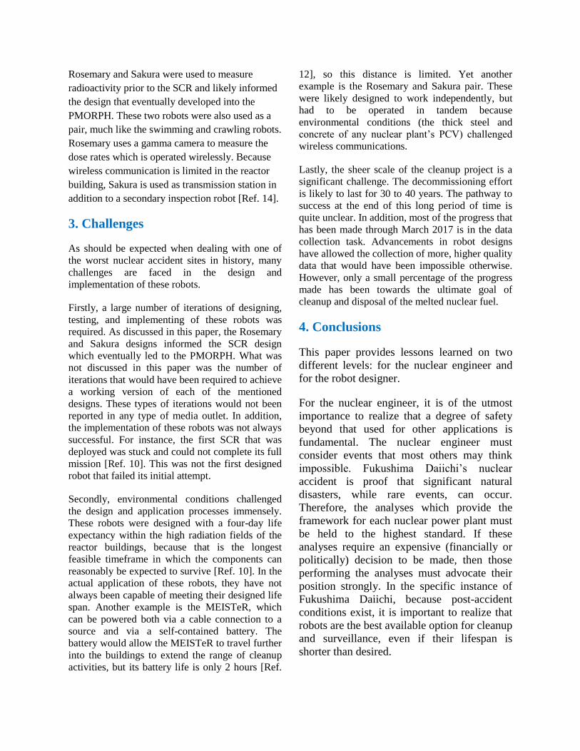
Rosemary and Sakura were used to measure

radioactivity prior to the SCR and likely informed

the design that eventually developed into the

PMORPH. These two robots were also used as a

pair, much like the swimming and crawling robots.

Rosemary uses a gamma camera to measure the

dose rates which is operated wirelessly. Because

wireless communication is limited in the reactor

building, Sakura is used as transmission station in

addition to a secondary inspection robot [Ref. 14].

3. Challenges

As should be expected when dealing with one of

the worst nuclear accident sites in history, many

challenges are faced in the design and

implementation of these robots.

Firstly, a large number of iterations of designing,

testing, and implementing of these robots was

required. As discussed in this paper, the Rosemary

and Sakura designs informed the SCR design

which eventually led to the PMORPH. What was

not discussed in this paper was the number of

iterations that would have been required to achieve

a working version of each of the mentioned

designs. These types of iterations would not been

reported in any type of media outlet. In addition,

the implementation of these robots was not always

successful. For instance, the first SCR that was

deployed was stuck and could not complete its full

mission [Ref. 10]. This was not the first designed

robot that failed its initial attempt.

Secondly, environmental conditions challenged

the design and application processes immensely.

These robots were designed with a four-day life

expectancy within the high radiation fields of the

reactor buildings, because that is the longest

feasible timeframe in which the components can

reasonably be expected to survive [Ref. 10]. In the

actual application of these robots, they have not

always been capable of meeting their designed life

span. Another example is the MEISTeR, which

can be powered both via a cable connection to a

source and via a self-contained battery. The

battery would allow the MEISTeR to travel further

into the buildings to extend the range of cleanup

activities, but its battery life is only 2 hours [Ref.

12], so this distance is limited. Yet another

example is the Rosemary and Sakura pair. These

were likely designed to work independently, but

had to be operated in tandem because

environmental conditions (the thick steel and

concrete of any nuclear plant’s PCV) challenged

wireless communications.

Lastly, the sheer scale of the cleanup project is a

significant challenge. The decommissioning effort

is likely to last for 30 to 40 years. The pathway to

success at the end of this long period of time is

quite unclear. In addition, most of the progress that

has been made through March 2017 is in the data

collection task. Advancements in robot designs

have allowed the collection of more, higher quality

data that would have been impossible otherwise.

However, only a small percentage of the progress

made has been towards the ultimate goal of

cleanup and disposal of the melted nuclear fuel.

4. Conclusions

This paper provides lessons learned on two

different levels: for the nuclear engineer and

for the robot designer.

For the nuclear engineer, it is of the utmost

importance to realize that a degree of safety

beyond that used for other applications is

fundamental. The nuclear engineer must

consider events that most others may think

impossible. Fukushima Daiichi’s nuclear

accident is proof that significant natural

disasters, while rare events, can occur.

Therefore, the analyses which provide the

framework for each nuclear power plant must

be held to the highest standard. If these

analyses require an expensive (financially or

politically) decision to be made, then those

performing the analyses must advocate their

position strongly. In the specific instance of

Fukushima Daiichi, because post-accident

conditions exist, it is important to realize that

robots are the best available option for cleanup

and surveillance, even if their lifespan is

shorter than desired.

For the robot designer, it is important to

balance simplicity and complexity and

recognize that intense technical rigor is

required to achieve a working design.

Simplicity and complexity are best balanced

by analyzing the needs of a particular job. For

instance, the SCR had a specialized mission of

data collection that was successfully

completed with few components or inputs. In

contrast, the MHI-MEISTeR had a general

mission of cleanup that was successfully

completed with many components,

attachments, etc. Intense technical rigor is

required, as seen by the slow, incremental

improvements in the various robot designs

presented in this paper. However, it is

important to realize that simple analyses (i.e.

similar to those shown in Appendix A) can

provide keen insights to robot design.

References

1. The Great East Japan Earthquake and

Current Status of Nuclear Power

Stations.

http://www.tepco.co.jp/en/nu/fukushim

a-np/f1/images/f12np-gaiyou_e_1.pdf

2. Kadota, Ry sh . “On the Brink: The

Inside Story of Fukushima Daiichi.”

Fukuoka, Japan: Kurodahan, 2014.

Print.

3. 2011 Japan Earthquake-Tsunami Fast

Facts.

http://www.cnn.com/2013/07/17/world

/asia/japan-earthquake---tsunami-fast-

facts/

4. TEPCO Plant Overview.

http://www.tepco.co.jp/en/challenge/en

ergy/nuclear/pdf/plants-e.pdf

5. Definition of Sievert.

http://www.dictionary.com/browse/sie

vert

6. 2012 Status of Fukushima Daiichi

Nuclear Power Station.


a-np/f1/images/f12np-gaiyou_e_4.pdf

7. Current Radiation Dose measured at

Monitoring Post of Fukushima Daiichi

Nuclear Power Station.


a-np/f1/index-e.html

8. Unit 1 Primary Containment Vessel

Internal Investigation. March 27, 2017.


a-

np/handouts/2017/images/handouts_17

0327_01-e.pdf

9. Unit 2 Primary Containment Vessel

Investigation at Fukushima Daiichi

Nuclear Power Station (By the self-

propelled investigation device).

February 15, 2017.


a-

np/handouts/2017/images/handouts_17

0215_01-e.pdf

10. Survey Device (Shape-changing

Robot) Deployed to Inspect Interior of

Primary Containment Vessel (PCV).

April 20, 2015.

http://irid.or.jp/en/research/20150420/

11. "MEISTeR" Remote Control Robot

Completes Demonstration Testing At

Fukushima Daiichi Nuclear Power

Station. Feb. 20, 2014.

http://www.mhi.com/news/story/14022

01775.html

12. Robots working inside the buildings at

Fukushima Daiichi NPS (Part II) MHI-

MEISTeR.

http://irid.or.jp/en/research/meister/


Fukushima Daiichi NPS (Part III)

Swimming robot & Crawling robot.

http://irid.or.jp/en/research/gengorov_t

rydiver/


Fukushima Daiichi NPS Rosemary &

Sakura.

http://irid.or.jp/en/research/rosemary_s

akura/

http://www.tepco.co.jp/en/nu/fukushima-np/f1/images/f12np-gaiyou_e_1.pdf


http://www.cnn.com/2013/07/17/world/asia/japan-earthquake---tsunami-fast-facts/



http://www.tepco.co.jp/en/challenge/energy/nuclear/pdf/plants-e.pdf

http://www.tepco.co.jp/en/challenge/energy/nuclear/pdf/plants-e.pdf

http://www.dictionary.com/browse/sievert

http://www.dictionary.com/browse/sievert



http://www.tepco.co.jp/en/nu/fukushima-np/f1/index-e.html

http://www.tepco.co.jp/en/nu/fukushima-np/f1/index-e.html

http://www.tepco.co.jp/en/nu/fukushima-np/handouts/2017/images/handouts_170327_01-e.pdf








http://irid.or.jp/en/research/20150420/

http://www.mhi.com/news/story/1402201775.html

http://www.mhi.com/news/story/1402201775.html

http://irid.or.jp/en/research/meister/

http://irid.or.jp/en/research/gengorov_trydiver/

http://irid.or.jp/en/research/gengorov_trydiver/

http://irid.or.jp/en/research/rosemary_sakura/

http://irid.or.jp/en/research/rosemary_sakura/

Appendix A: Brief Analysis of PMORPH

Topology and Coordinate Frames:

Mobility: One Free Rotation of the Revolute, Two Rotations of the Universal

Kinematic Setup: Two-Link Manipulator in 2-D

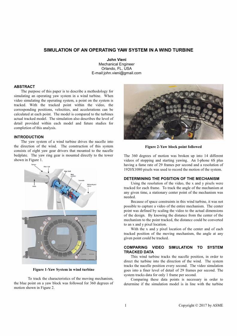
1 Copyright © 2017 by ASME

SIMULATION OF AN OPERATING YAW SYSTEM IN A WIND TURBINE

John VieniMechanical Engineer

Orlando, FL, USAE-mail:[email protected]

ABSTRACTThe purpose of this paper is to describe a methodology for

simulating an operating yaw system in a wind turbine. Whenvideo simulating the operating system, a point on the system istracked. With the tracked point within the video, thecorresponding positions, velocities, and accelerations can becalculated at each point. The model is compared to the turbinesactual tracked model. The simulation also describes the level ofdetail provided within each model and future studies forcompletion of this analysis.

INTRODUCTIONThe yaw system of a wind turbine drives the nacelle into

the direction of the wind. The construction of this systemconsists of eight yaw gear drivers that mounted to the nacellebedplate. The yaw ring gear is mounted directly to the towershown in Figure 1.

Figure 1-Yaw System in wind turbine

To track the characteristics of the moving mechanism,the blue point on a yaw block was followed for 360 degrees ofmotion shown in Figure 2.

Figure 2-Yaw block point followed

The 360 degrees of motion was broken up into 14 differentvideos of stopping and starting yawing. An I-phone 6S plushaving a fame rate of 29 frames per second and a resolution of1920X1080 pixels was used to record the motion of the system.

DETERMINING THE POSITION OF THE MECHANISMUsing the resolution of the video, the x and y pixels were

tracked for each frame. To track the angle of the mechanism atany given time, a stationary center point of the mechanism wasneeded.

Because of space constraints in this wind turbine, it was notpossible to capture a video of the entire mechanism. The centerpoint was defined by scaling the video to the actual dimensionsof the design. By knowing the distance from the center of themechanism to the point tracked, the distance could be convertedto an x and y pixel location.

With the x and y pixel location of the center and of eachtracked position of the moving mechanism, the angle at anygiven point could be tracked.

COMPARING VIDEO SIMULATION TO SYSTEMTRACKED DATA

This wind turbine tracks the nacelle position, in order todirect the turbine into the direction of the wind. The systemtracks the nacelle position every second. The video simulationgoes into a finer level of detail of 29 frames per second. Thesystem tracks data for only 1 frame per second.

Comparing these data points is necessary in order todetermine if the simulation model is in line with the turbine


tracked data. The comparison is also used to evaluate thebehavior of the system.

APPLYING A SAVITISKY-GOLAY FILTERA 7 point Savitisky-Golay filter was applied to the

simulation data and the turbine data. It was applied to removethe noise from the data set. To affectively apply this filter onemust calculate the position, velocity, acceleration, and jerk ateach time step (h) Eq. (1). At the first three time step one isunable to use the 7 point filter without interpolating the positionEq. (1a), velocity Eq. (1b), acceleration (1c), and jerk (1d),from the fourth time step (x4).

xi* = (- 2 xi+3+3 xi+2+ 6 xi+1+7 xi+6 xi-1+3 xi-2 -2 xi-3 ) / 21 (1a)

x i* = (- 22 xi+3+67 xi+2+58 xi+1-58 xi-1 -67 xi-2+22 xi-3)/252h(1b)

x i* = ( 5 xi+3 - 3 xi+1 - 4 xi - 3 xi-1 + 5 xi-3 ) / 42 h2 (1c)

x i* = ( xi+3 - xi+2 - xi-1 + xi-1 + xi-2 - xi-3 ) / 6 h3 (1d)

After determining the values at the fourth time step,interpolator values can be calculated for the first three timesteps (h) Eq. (2).

b0 = x4* (2a)

b1 = x 4* h (2b)

b2 = x 4* h2 / 2 (2c)

b3 = x 4* h3 / 6 (2d)

Once the interpolator values are calculated the positionEq. (3), velocity Eq. (4), acceleration Eq. (5), and jerk Eq. (6)can be calculated for the first three time steps.

x1*= b0-3b1+9b2 27b3 (3a)

x2*= b0-2b1+4b2 8b3 (3b)

x3*=b0-b1+b2-b3 (3c)

x 1* = (b1 6b2+27b3)/ h (4a)

x 2* = (b1 4b2+12b3)/ h (4b)

x 3* = (b1 2b2+3b3)/ h (4c)

x 1* = (2b2 18b3)/ h2 (5a)

x 2* = (2b2 12b3)/ h2 (5b)

x 3* = (2b2 6b3)/ h2 (5c)

x 1* = x 4

* (6a)x 2

* = x 4* (6b)

x 3* = x 4

* (6c)

Additionally, one is unable to use the Savitisky-GolayFilter on the last three time steps without interpolating theposition Eq. (1a), velocity Eq. (1b), acceleration (1c), and jerk

(1d), from the fourth to last time step (xn-3). The interpolatorsused for the last three time steps (h) are described in Eq. (7).

b0 = xn-3* (7a)

b1 = x n-3* h (7b)

b2 = x n-3* h2 / 2 (7c)

b3 = x n-3* h3 / 6 (7d)

Once the interpolator values are calculated one can calculate theposition Eq. (8), velocity Eq. (9), acceleration Eq. (10), and jerkEq. (11) for the last three time steps.

xn-2* = b0+b1+b2+b3 (8a)

xn-1* = b0+2b1+4b2+8b3 (8b)

xn* = b0+3b1+9b2+27b3 (8c)

x n-2* = (b1+2b2+3b3) / h (9a)

x n-1* = (b1+4b2+12b3) / h (9b)

x n* = (b1+6b2+27b3) / h (9c)

x n-2* = (2b2+6b3) / h2 (10a)

x n-1* = (2b2+12b3) / h2 (10b)

x n* = (2b2+18b3) / h2 (10c)

x n-2* = x n-3

* (11a)x n-1

* = x n-3* (11b)

x n* = x n-3

* (11c)

ANAYLSIS OF THE SIMULATIONThe initial analysis was done from 0 to 27 degrees. The

simulated data showed that the position did not change linearly.The position of the system seemed to be very choppy during thefirst 10 seconds and then after the initial 10 seconds the systemstarts to smooth, shown in Figure 2.

Figure 2-Video simulated position

seemed to be moving in a linear pattern shown in Figure 3.


Figure 3-Turbine simulated position

After applying the Savitisky-Golay filter the positionof the simulated data seemed to show the position in finerdetail, shown in Figure 4. The filter exemplifies the variabilityin the position of the nacelle in between the 7 to 9 second range.

Figure 4-Video simulated position Savitisky-Golay filter

When analyzing the turbine simulated position, theSavitisky-Golay filter does not transform the data very much.The position of the nacelle system changes linearly, shown inFigure 5.

Figure 5-Turbine simulated position Savitisky-Golay filter

When studying the velocity and acceleration, theanalysis started to show significant differences between models.In the simulated video, the speed of the system was very volatileranging from -2 to 2 degrees per second, shown in Figure 6.Based on the design of the system it does not seem very likelythat the system could be operating at these speeds. Someexternal forces would have to be present to allow for the systemto change position that rapidly.

Figure 6-Video simulated velocity Savitisky-Golay filter

The turbine simulated speed is roughly between 0.4-0.5 degrees per second, shown in Figure 7. This is more in linewith the designed yawing speed of this turbine.


Figure 7-Turbine simulated velocity Savitisky-Golay filter

The acceleration analysis of the simulated videoshowed to be very volatile as well. The acceleration rangedfrom 15 to -15 degrees per second squared, shown in Figure 8.

Figure 8-Video simulated acceleration Savitisky-Golay filter

, itshows that the system speed up during start up and sloweddown during shut down. Additionally, while yawing, the speeddid not seem to accelerate very much, shown in Figure 9. Thisaligns with the logic of the turbines system.

Figure 9-Turbine simulated acceleration Savitisky-Golayfilter

From the position analysis the models looks fairly thesame, but when looking at the velocity and acceleration the

simulation.

CONCLUSIONSBased on the results found from the simulated model

compared to the turbines model, the results from this simulationare inconclusive. There were several things that occurredduring the simulation model that does not allow for concreateconclusions.

The first problem that I ran into was filming thismechanism. In order to film this mechanism, I had to liedirectly on the yaw deck. Even with this visual, I was only ableto capture part of the mechanism in the video. I was able tocapture the moving mechanism with a partial frame but it stillleads me into my second problem with this model.

When determining the position of the moving point, Ihad to scale the center point of the mechanism in order to getroughly an idea at which angle the mechanism was at. Because Iwas lying directly on the yaw deck my video picture was notalways show from the same location as my hands could havebeen moving from time to time. This allowed for variedpositions and an extra third dimension.

Because of the radical results of the simulation, moreinvestigation will be done. When first looking into this it wasthought that the simulation model should match with the turbinemodel but show a finer level of detail of what is happening.

Instead, the results between simulations were totallydifferent. If this is the actual case, the behavior of the systemcan be better defined from filmed simulations of the turbine.

The next steps for completing this analysis are tofigure out how to simulate the model with a fixed cameralocation that encompasses the entire system. This will remove


the scaling error as well as the shaky camera errors. Theresults can then be compared to the initial analysis and the

REFERENCESNotes_05_02 H J SommerSiemens 2.3-108 Turbine

ME 581: Simulation of Mechanical Systems Experimental Analysis of a Various Pool Shots

Grant Week es

Abstract

There are various shooting styles available to a pool player. However, during each shot, the exact angle, speed, and position of the pool cue must be considered to ensure accuracy. Certain shots have a higher focus on power, such as a breaking shot. Others still focus on angle and position, like a draw shot. This report examines the kinematics of a pool cue-tip when making various strikes. The intent of this report is to provide a basic analysis of the shots, providing benchmark values for speed, acceleration, and jerk of each shot. The experiment also was intended to develop improved capabilities with motion capture methods.

2. Methodology

2.1. Experiment

For this experiment I recorded three types of shots recording three strikes for each type, a total of nine recordings. For each shot, 4 felt markers were placed on the shooter, allowing tracking of joint positions. The landmarks are as follows:

LM=1 at Shoulder

LM=2 at Elbow LM=3 at Wrist LM=4 at First Knuckle LM=5 at Cue Tip

The intent was to vary the shot type and obtain multiple recordings of each shot type in order to account for some inconsistency in the shots. Due to the physical arrangement of the pool table and the room it was in, shooting with my right, non-

dominant hand, was necessary. Additionally, the pool table was not the traditional green felt, reducing the contrast between some of the felt markers and the background. A friend began and ended each recording to minimize the amount of unnecessary footage taken for each recording.

2.2. Motion Capture

Once each recording was made, still frames were ripped from each video using vlc software. Each clip was between four and seven seconds long. The camera recorded each video at thirty frames per second, resulting in approximately one-hundred and seventy frames per video-clip. The tpsdig software was then used to compile and mark the frames with landmarks at each felt dot/ at the cue tip. Marking each video’s frames and extracting the data to a usable form was a very laborious process, resulting in the coordinates for each landmark in each frame of each video.

2.3. Data

The coordinates were plotted for each shot, providing an image of the practice strokes and strike taken. These images are shown in Figures 2.1 through 2.9.

Figure 2.1: Point positions for 1st breaking shot

Figure 2.2: Point positions for 2nd breaking shot

Figure 2.3: Point positions for 3rd breaking shot

Figure 2.4: Point positions for 1st draw shot

Figure 2.5: Point positions for 2nd draw shot

Figure 2.6: Point positions for 3rd draw shot

Figure 2.7: Point positions for 1st Normal shot

Figure 2.8: Point positions for 2nd Normal shot

Figure 2.9: Point positions for 3rd Normal shot

3. Analysis

3.1 Position Data

With the position data, I was able to calculate the average practice stroke length and the length of the shot, including follow through, in the horizontal direction, shown in Table 3.1.

Shot Type Shot Attempt Stroke Type Length (inches) Breaks 1 Avg Practice 5.5

Strike 16.5 2 Avg Practice 4.5

Strike 15 3 Avg Practice 5.5

Strike 17.5 Normal Shots

1 Avg Practice 4.5 Strike 13

2 Avg Practice 5.5 Strike 11.5

3

Avg Practice 4.5 Strike 17

Draw Shots

1 Avg Practice 5.5 Strike 10

2 Avg Practice 7 Strike 11

3

Avg Practice 5 Strike 13

Table 3.1: stroke lengths for each strike & practice set

My initial review of the position data, and my experience performing the motion capture landmark placement, led me to believe that determination of a precise strike location was not possible due to the relatively low frame rate compared to the speed of the pool cue. However, upon further review of the data, I found that this was not necessarily the case. Table 2 shows the cue tip location for each practice shot (at full extension) and the cue tip location for the frames immediately before and after each strike (for improved granularity, these values are in pixels: 1 pixel=0.0785 inches).

Stroke (practice number shown as decimal)

x-position(s) y-position(s)

Break 1.1 689 419 Break 1.2 703 417 Break 1.3 708 416

Break 1 654, 724 422, 421 Break 2.1 669 420 Break 2.2 652 420 Break 2.3 654 420 Break 2.4 683 419 Break 2.5 683 416

Break 2 667, 729 415,414 Break 3.1 711 421 Break 3.2 726 418

Break 3 679, 741 424, 423 Normal 1.1 706 419 Normal 1.2 705 420

Normal 1 702, 728 418, 416 Normal 2.1 691 418 Normal 2.2 689 418 Normal 2.3 696 417

Normal 2 657, 710 418, 411 Normal 3.1 704 420 Normal 3.2 710 418

Normal 3 709, 735 420, 419 Draw 1.1 697 415 Draw 1.2 710 412

Draw 1 704, 735 413, 410 Draw 2.1 676 414 Draw 2.2 683 413 Draw 2.3 684 413

Draw 2 662, 691 417,411 Draw 3.1 691 412 Draw 3.2 692 412

Draw 3 686, 725 413, 411 Table 2: Practice targets and strike points

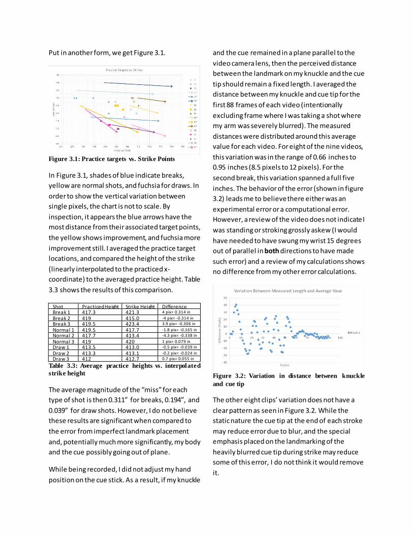
Put in another form, we get Figure 3.1.

Figure 3.1: Practice targets vs. Strike Points

In Figure 3.1, shades of blue indicate breaks, yellow are normal shots, and fuchsia for draws. In order to show the vertical variation between single pixels, the chart is not to scale. By inspection, it appears the blue arrows have the most distance from their associated target points, the yellow shows improvement, and fuchsia more improvement still. I averaged the practice target locations, and compared the height of the strike (linearly interpolated to the practiced x-coordinate) to the averaged practice height. Table 3.3 shows the results of this comparison.

Shot Practiced Height Strike Height Difference Break 1 417.3 421.3 4 pix= 0.314 in Break 2 419 415.0 -4 pix= -0.314 in Break 3 419.5 423.4 3.9 pix= -0.306 in Normal 1 419.5 417.7 -1.8 pix= -0.165 in Normal 2 417.7 413.4 -4.3 pix= -0.338 in Normal 3 419 420 1 pix= 0.079 in Draw 1 413.5 413.0 -0.5 pix= -0.039 in Draw 2 413.3 413.1 -0.2 pix= -0.024 in Draw 3 412 412.7 0.7 pix= 0.055 in

Table 3.3: Average practice heights vs. interpolated strike height

The average magnitude of the “miss” for each type of shot is then 0.311” for breaks, 0.194”, and 0.039” for draw shots. However, I do not believe these results are significant when compared to the error from imperfect landmark placement and, potentially much more significantly, my body and the cue possibly going out of plane.

While being recorded, I did not adjust my hand position on the cue stick. As a result, if my knuckle

and the cue remained in a plane parallel to the video camera lens, then the perceived distance between the landmark on my knuckle and the cue tip should remain a fixed length. I averaged the distance between my knuckle and cue tip for the first 88 frames of each video (intentionally excluding frame where I was taking a shot where my arm was severely blurred). The measured distances were distributed around this average value for each video. For eight of the nine videos, this variation was in the range of 0.66 inches to 0.95 inches (8.5 pixels to 12 pixels). For the second break, this variation spanned a full five inches. The behavior of the error (shown in figure 3.2) leads me to believe there either was an experimental error or a computational error. However, a review of the video does not indicate I was standing or stroking grossly askew (I would have needed to have swung my wrist 15 degrees out of parallel in both directions to have made such error) and a review of my calculations shows no difference from my other error calculations.

Figure 3.2: Variation in distance between knuckle and cue tip

The other eight clips’ variation does not have a clear pattern as seen in Figure 3.2. While the static nature the cue tip at the end of each stroke may reduce error due to blur, and the special emphasis placed on the landmarking of the heavily blurred cue tip during strike may reduce some of this error, I do not think it would remove it.

3.2 Speed Data

Next I adapted a standard 3-point central derivative and 5-point central derivative to calculate the speed of each point at each frame (vice velocity in the horizontal and vertical directions) as shown in Equations 3.1 and 3.2.

𝑆𝑆𝑆𝑆𝑆𝑆𝑆𝑆𝑆𝑆𝑛𝑛3−𝑝𝑝𝑝𝑝 = ��𝑥𝑥𝑛𝑛+1− 𝑥𝑥𝑛𝑛−1

2 ∗ 𝑆𝑆𝑑𝑑 �2

+ �𝑦𝑦𝑛𝑛+1 − 𝑦𝑦𝑛𝑛−1

2 ∗ 𝑆𝑆𝑑𝑑 �2∗𝑖𝑖𝑖𝑖𝑖𝑖ℎ𝑆𝑆𝑒𝑒𝑆𝑆𝑖𝑖𝑥𝑥𝑆𝑆𝑝𝑝

Equation 3.1: Three point speed

𝑺𝑺𝑺𝑺𝑺𝑺𝑺𝑺𝑺𝑺𝒏𝒏𝟓𝟓−𝑺𝑺𝒑𝒑 =

��−𝒙𝒙𝒏𝒏+𝟐𝟐 + 𝟖𝟖𝒙𝒙𝒏𝒏+𝟏𝟏 − 𝟖𝟖𝒙𝒙𝒏𝒏−𝟏𝟏 + 𝒙𝒙𝒏𝒏+𝟏𝟏

𝟏𝟏𝟐𝟐 ∗ 𝑺𝑺𝒑𝒑�𝟐𝟐

+ �−𝒚𝒚𝒏𝒏+𝟐𝟐 + 𝟖𝟖𝒚𝒚𝒏𝒏+𝟏𝟏 − 𝟖𝟖𝒚𝒚𝒏𝒏−𝟏𝟏 + 𝒚𝒚𝒏𝒏+𝟏𝟏

𝟏𝟏𝟐𝟐 ∗ 𝑺𝑺𝒑𝒑�𝟐𝟐

∗𝒊𝒊𝒏𝒏𝒊𝒊𝒊𝒊𝑺𝑺𝒊𝒊𝑺𝑺𝒊𝒊𝒙𝒙𝑺𝑺𝒑𝒑

Equation 3.2: Five point speed

This resulted in 18 graphs, however the plots of each strike’s speed are not particularly necessary for further analyses. Representative graphs from the first break are shown in Figures 3.3 and 3.4, below.

Figure 3.3: First break speeds (3-pt derivative)

Figure 3.4: First break speeds (5-pt derivative)

Note that each pair of peaks represents the drawing back and then the moving forward of the cue as the plot depicts the speed. Figure 3.5 shows a side-by-side comparison of the two methods of differentiation for the knuckle landmark’s speed during this first break.

Figure 3.5: Comparison of differentiation methods

It is readily observable that the strike event last approximately five to seven frames (0.3925 seconds to 0.5495 seconds). Because of this, continued use of a 5-point differentiation method would quickly lead to parameters of the strike event being influenced by data from other events of the clip (by the time I calculated jerk using 5-point differentiations for scalar acceleration and jerk, every single point of the strike event would have some weighting from points before or after the strike event). For this reason, I abandoned further use of 5-point differentiations.

The speed reached for each strike is shown in Table 3.4.

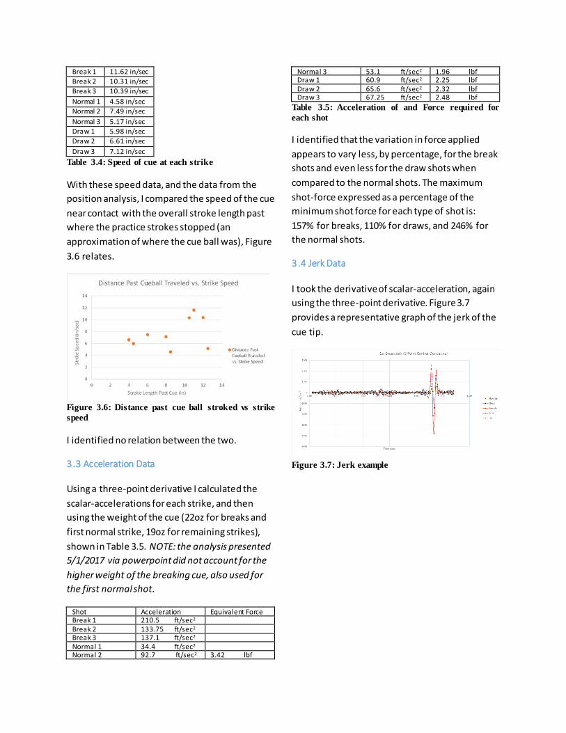
Break 1 11.62 in/sec Break 2 10.31 in/sec Break 3 10.39 in/sec Normal 1 4.58 in/sec Normal 2 7.49 in/sec Normal 3 5.17 in/sec Draw 1 5.98 in/sec Draw 2 6.61 in/sec Draw 3 7.12 in/sec

Table 3.4: Speed of cue at each strike

With these speed data, and the data from the position analysis, I compared the speed of the cue near contact with the overall stroke length past where the practice strokes stopped (an approximation of where the cue ball was), Figure 3.6 relates.

Figure 3.6: Distance past cue ball stroked vs strike speed

I identified no relation between the two.

3.3 Acceleration Data

Using a three-point derivative I calculated the scalar-accelerations for each strike, and then using the weight of the cue (22oz for breaks and first normal strike, 19oz for remaining strikes), shown in Table 3.5. NOTE: the analysis presented 5/1/2017 via powerpoint did not account for the higher weight of the breaking cue, also used for the first normal shot.

Shot Acceleration Equivalent Force Break 1 210.5 ft/sec2 Break 2 133.75 ft/sec2

Break 3 137.1 ft/sec2 Normal 1 34.4 ft/sec2 Normal 2 92.7 ft/sec2 3.42 lbf

Normal 3 53.1 ft/sec2 1.96 lbf Draw 1 60.9 ft/sec2 2.25 lbf Draw 2 65.6 ft/sec2

2.32 lbf Draw 3 67.25 ft/sec2

2.48 lbf Table 3.5: Acceleration of and Force required for each shot

I identified that the variation in force applied appears to vary less, by percentage, for the break shots and even less for the draw shots when compared to the normal shots. The maximum shot-force expressed as a percentage of the minimum shot force for each type of shot is: 157% for breaks, 110% for draws, and 246% for the normal shots.

3.4 Jerk Data

I took the derivative of scalar-acceleration, again using the three-point derivative. Figure 3.7 provides a representative graph of the jerk of the cue tip.

Figure 3.7: Jerk example

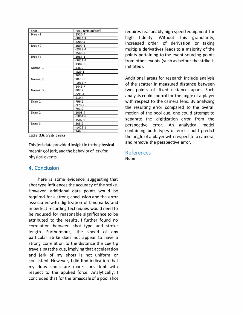
Shot Peak Jerks (in/sec3) Break 1 2526.4

-3824.3 2200.4

Break 2 1609.1 -2989.4 2548.8

Break 3 1983.1 -3012.6 1302.6

Normal 1 446.9 -529.1 369.4

Normal 2 1078.5 -1963.7 1449.7

Normal 3 802.7 -591.4 510.4

Draw 1 796.5 -978.2 793.9

Draw 2 1008.4 -1861.6 1507.9

Draw 3 805.2 -1421.1 1469.6

Table 3.6: Peak Jerks

This jerk data provided insight in to the physical meaning of jerk, and the behavior of jerk for physical events.

4. Conclusion

There is some evidence suggesting that shot type influences the accuracy of the strike. However, additional data points would be required for a strong conclusion and the error associated with digitization of landmarks and imperfect recording techniques would need to be reduced for reasonable significance to be attributed to the results. I further found no correlation between shot type and stroke length. Furthermore, the speed of any particular strike does not appear to have a strong correlation to the distance the cue tip travels past the cue, implying that acceleration and jerk of my shots is not uniform or consistent. However, I did find indication that my draw shots are more consistent with respect to the applied force. Analytically, I concluded that for the timescale of a pool shot

requires reasonably high speed equipment for high fidelity. Without this granularity, increased order of derivation or taking multiple derivatives leads to a majority of the points pertaining to the event sourcing points from other events (such as before the strike is initiated). Additional areas for research include analysis of the scatter in measured distance between two points of fixed distance apart. Such analysis could control for the angle of a player with respect to the camera lens. By analyzing the resulting error compared to the overall motion of the pool cue, one could attempt to separate the digitization error from the perspective error. An analytical model containing both types of error could predict the angle of a player with respect to a camera, and remove the perspective error.

References None

me 581: simulation of mechanical systems inverse ... · mechanism. link 1 – solar panel frame...

Documents