ME-662 CONVECTIVE HEAT AND MASSTRANSFER

A. W. DateMechanical Engineering Department

Indian Institute of Technology, BombayMumbai - 400076

India

LECTURE-29 PREDICTION OF TURBULENT FLOWS

() March 26, 2012 1 / 21

LECTURE-29 PREDICTION OFTURBULENT FLOWS

1 Prediction of Cf ,x ( Ext Bls )1 Integral Method2 Complete Laminar-Transition-Turbulent BL3 Similarity Method

2 Prediction of f ( Internal Flows )- Use of Law of the wall

() March 26, 2012 2 / 21

Integral Method - Ext BLs - 1 L29( 119)

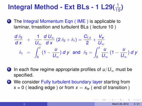
1 The Integral Momentum Eqn ( IME ) is applicable tolaminar, trnasition and turbulent BLs ( lecture 10 )

d δ2

d x+

1U∞

d U∞d x

(2 δ2 + δ1) =Cf ,x

2+

Vw

U∞

δ1 =

∫ δ

0(1− u

U∞) d y and δ2 =

∫ δ

0

uU∞

(1− uU∞

) d y

2 In each flow regime appropriate profiles of u/U∞ must bespecified.

3 We consider Fully turbulent boundary layer starting fromx = 0 ( leading edge ) or from x = xte ( end of transition )

() March 26, 2012 3 / 21

Power Law Assumption - L29( 219)

1 Evaluations of δ1 and δ2 are negligibly affected in TBLswhen Laminar sub-layer and transition layers are ignored.

2 Then, only fully turbulent vel profile ( universal logarithmiclaw ( inner ) + law of the wake ( outer ) ) suffices.

3 However, integration as well as evaluation ofCf ,x = τw/(ρ U2

∞) becomes extremely involved.4 Hence, for an impermeable smooth wall ( vw = 0 ), a

power-law is assumed

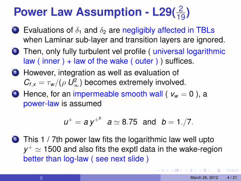
u+ = a y+ba ' 8.75 and b = 1./7.

5 This 1 / 7th power law fits the logarithmic law well uptoy+ ' 1500 and also fits the exptl data in the wake-regionbetter than log-law ( see next slide )

() March 26, 2012 4 / 21

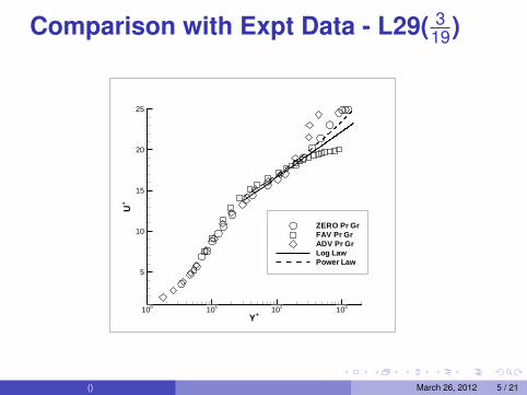
Comparison with Expt Data - L29( 319)

Y+

U+

100 101 102 103

5

10

15

20

25

ZERO Pr GrFAV Pr GrADV Pr GrLog LawPower Law

() March 26, 2012 5 / 21

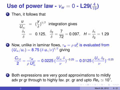
Use of power law - vw = 0 - L29( 419)

1 Then, it follows that

uU∞

= (yδ

)1/7 integration gives

δ1

δ= 0.125,

δ2

δ=

772

= 0.097, H =δ1

δ2= 1.29

2 Now, unlike in laminar flows, τw = ρ u2τ is evaluated from

(U∞/uτ ) = 8.75 (δ uτ/ν)1/7 giving

Cf ,x

2=

τw

ρ U2∞

= 0.0225 (U∞ δν

)−0.25 = 0.0125 (U∞ δ2

ν)−0.25

3 Both expressions are very good approximations to mildlyadv pr gr through to highly fav. pr. gr and upto Rex ' 107.

() March 26, 2012 6 / 21

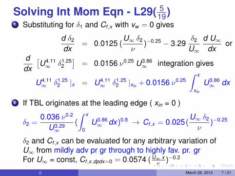
Solving Int Mom Eqn - L29( 519)

1 Substituting for δ1 and Cf ,x with vw = 0 gives

d δ2

dx= 0.0125 (

U∞ δ2

ν)−0.25 − 3.29

δ2

U∞d U∞

dxor

ddx

[U4.11∞ δ1.25

2

]= 0.0156 ν0.25 U3.86

∞ integration gives

U4.11∞ δ1.25

2 |x = U4.11∞ δ1.25

2 |xin + 0.0156 ν0.25∫ x

xin

U3.86∞ dx

2 If TBL originates at the leading edge ( xin = 0 )

δ2 =0.036 ν0.2

U3.29∞

(

∫ x

0U3.86∞ dx)0.8 → Cf ,x = 0.025(

U∞ δ2

ν)−0.25

δ2 and Cf ,x can be evaluated for any arbitrary variation ofU∞ from mildly adv pr gr through to highly fav. pr. grFor U∞ = const, Cf ,x ,dpdx=0 = 0.0574 (U∞ x

ν)−0.2

() March 26, 2012 7 / 21

Highly Adv Pr Gr & vw - L29( 619)

1 For these cases, IME is again written asd δ2

d x+

δ2

U∞d U∞d x

(2 + H) =Cf ,x

2+

Vw

U∞2 Now, H and Cf ,x are modeled as

H =

[1−G

√Cf ,x/2.0

]−1

G ' 6.2 (1.43 + β + B)0.482, β =δ1

τw

dpdx, B =

vw/U∞Cf ,x/2

Cf ,x = Cf ,x ,dpdx=0 × (1 + 0.2 β)−1 (Crawford and Kays), orCf ,x = 0.246× 10−0.678 H × Re−0.268

δ2(Ludwig and Tilman)

Cf ,x = 0.336× {ln (854.6 δ2/yre)}−2 (rough surface)

Valid for −1.43 < β + B < 12. Iterative soln of IME isrequired.

() March 26, 2012 8 / 21

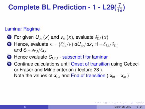
Complete BL Prediction - 1 - L29( 719)

Laminar Regime1 For given U∞ (x) and vw (x), evaluate δ2,l (x)2 Hence, evaluate κ = (δ2

2,l/ν) dU∞/dx , H = δ1,l/δ2,l

and S = δ2,l/δ4,l .3 Hence evaluate Cf ,x ,l - subscript l for laminar4 Continue calculations until Onset of transition using Cebeci

or Fraser and Milne criterion ( lecture 28 ).Note the values of xt ,s and End of transition ( xte − xts )

() March 26, 2012 9 / 21

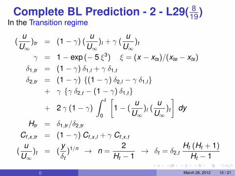
Complete BL Prediction - 2 - L29( 819)

In the Transition regime

(u

U∞)tr = (1− γ) (

uU∞

)l + γ (u

U∞)t

γ = 1− exp (− 5 ξ3) ξ = (x − xts)/(xte − xts)

δ1,tr = (1− γ) δ1,l + γ δ1,t

δ2,tr = (1− γ) {(1− γ) δ2,l − γ δ1,l}+ γ {γ δ2,t − (1− γ) δ1,t}

+ 2 γ (1− γ)

∫ δ

0

[1− (

uU∞

)l (u

U∞)t

]dy

Htr = δ1,tr/δ2,tr

Cf ,x ,tr = (1− γ) Cf ,x ,l + γ Cf ,x ,t

(u

U∞)t = (

yδt

)1/n → n =2

Ht − 1→ δt = δ2,t

Ht (Ht + 1)

Ht − 1

() March 26, 2012 10 / 21

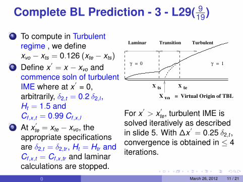
Complete BL Prediction - 3 - L29( 919)

1 To compute in Turbulentregime , we definexvo − xts = 0.126 (xte − xts)

2 Define x ′= x − xvo and

commence soln of turbulentIME where at x ′ = 0,arbitrarily, δ2,t = 0.2 δ2,l ,Ht = 1.5 andCf ,x ,t = 0.99 Cf ,x ,l

3 At x ′te = xte − xvo, the

appropriate specificationsare δ2,t = δ2,tr , Ht = Htr andCf ,x ,t = Cf ,x ,tr and laminarcalculations are stopped.

Laminar Transition Turbulent

X

= 0 = 1γ γ

X ts te

X vo = Virtual Origin of TBL

For x ′> x ′

te, turbulent IME issolved iteratively as describedin slide 5. With ∆x ′

= 0.25 δ2,t ,convergence is obtained in ≤ 4iterations.

() March 26, 2012 11 / 21

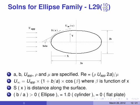
Solns for Ellipse Family - L29(1019)

U app S ( x )

Y2b

2a

beta

U 8 ( x )

X

1 a, b, Uapp, ρ and µ are specified. Re = (ρ Uapp 2a)/µ2 U∞ = Uapp × (1 + b/a)× cos (β) where β is function of x3 S ( x ) is distance along the surface.4 ( b / a ) > 0 ( Ellipse ), = 1.0 ( cylinder ), = 0 ( flat plate)

() March 26, 2012 12 / 21

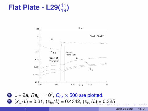
Flat Plate - L29(1119)

1 L = 2a, ReL = 107, Cf ,x × 500 are plotted.2 (xts/L) = 0.31, (xte/L) = 0.4342, (xvo/L) = 0.325

() March 26, 2012 13 / 21

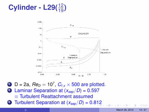
Cylinder - L29(1219)

1 D = 2a, ReD = 107, Cf ,x × 500 are plotted.2 Laminar Separation at (xsep/D) = 0.597≡ Turbulent Reattachment assumed

3 Turbulent Separation at (xsep/D) = 0.812() March 26, 2012 14 / 21

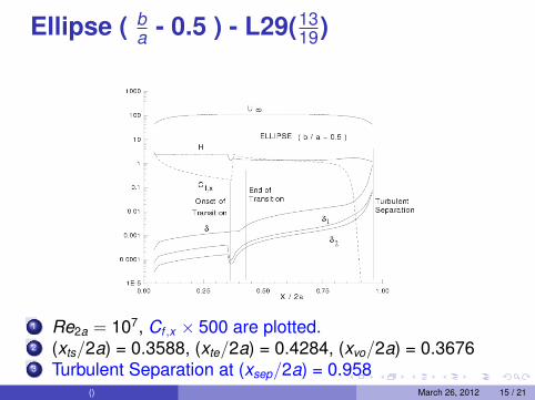
Ellipse ( ba - 0.5 ) - L29(13

19)

1 Re2a = 107, Cf ,x × 500 are plotted.2 (xts/2a) = 0.3588, (xte/2a) = 0.4284, (xvo/2a) = 0.36763 Turbulent Separation at (xsep/2a) = 0.958

() March 26, 2012 15 / 21

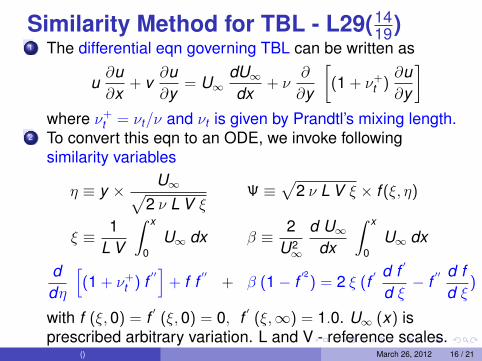
Similarity Method for TBL - L29(1419)

1 The differential eqn governing TBL can be written as

u∂u∂x

+ v∂u∂y

= U∞dU∞dx

+ ν∂

∂y

[(1 + ν+

t )∂u∂y

]where ν+

t = νt/ν and νt is given by Prandtl’s mixing length.2 To convert this eqn to an ODE, we invoke following

similarity variables

η ≡ y × U∞√2 ν L V ξ

Ψ ≡√

2 ν L V ξ × f (ξ, η)

ξ ≡ 1L V

∫ x

0U∞ dx β ≡ 2

U2∞

d U∞dx

∫ x

0U∞ dx

ddη

[(1 + ν+

t ) f′′]

+ f f′′

+ β (1− f′2

) = 2 ξ (f′ d f ′

d ξ− f

′′ d fd ξ

)

with f (ξ, 0) = f ′(ξ, 0) = 0, f ′

(ξ,∞) = 1.0. U∞ (x) isprescribed arbitrary variation. L and V - reference scales.

() March 26, 2012 16 / 21

Sim Meth for Eq. BLs - L29(1519)

1 The Eqn of previous slide can be used for flow over anellipse, for example, with U∞ = Uapp × (1 + b/a)× cos (β)and ν+

t = 0 ( Lam ) and ν+tr = (1− γ) + γ ν+

t ( Trans )2 When U∞ = C xm, ( Equilibrium BLs ) , we have

η = y ×√

(U∞ν x

) (m + 1

2)

ψ =

√(

2m + 1

) (U∞ ν x)× f (x , η)

ddη

[(1 + ν+

t ) f′′]

+ f f′′

+ (2m

m + 1) (1− f

′2)

= x (f′ df ′

dx− f

′′ dfdx

)

with f (x ,0) = f ′(x ,0) = 0, f ′

(x ,∞) = 1.0.

() March 26, 2012 17 / 21

Soln Procedure - L29(1619)

1 The presence of axial derivatives on the RHS requiresiterative solution.

2 Therefore, at first ∆x , Set RHS = 0 and solve 3rd orderODE to predict f, f ′ and f ′′ as functions of η

3 At subsequent ∆x ’s, evaluate the RHS from df/dx =(fx − fx−∆x )/∆x etc and solve the 3rd order ODE byRunge-Kutta method.

4 Using the new f, f ′ and f ′′ distributions, evaluate the RHSand Solve the ODE again

5 Go to step 3 until predicted f-distributions betweeniterations converge within a tolerance.

6 For further refinements of this method see Cebeci andCousteix, Modeling and Computation of Boundary-LayerFlows, 2nd ed, Springer, ( 2005 )

() March 26, 2012 18 / 21

F. D. Pipe Flow - 1 - L29(1719)

1 In lecture 26, it was shown that the log-law predicts the velprofile remarkably well upto the pipe center line . Then

u =2

R2

∫ R

0u r dr

u+ =2

R+2

∫ R+

0u+ (R+ − y+) dy+ → y = R − r

2 Since R+ = O ( 1000 ), contribution to the integral upto y+ =30 is negligible. Writing log-law as y+ = E−1 exp (κ u+) ,where E = 9.152 and κ = 0.41,

u+ =2 κ

ER+2

∫ u+cl

0u+{

R+ − E−1 exp (κ u+)}

exp (κ u+) du+

= u+cl −

32 κ

+2

κ E R+− 1κ E2 R+2 ' u+

cl −3

2 κwhere subscript cl = centerline

() March 26, 2012 19 / 21

F. D. Pipe Flow - 2 - L29(1819)

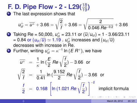
1 The last expression shows that

u+cl = u+ + 3.66 =

√2f

+ 3.66 =

√2

0.046 Re−0.2 + 3.66

2 Taking Re = 50,000, u+cl = 23.11 or (u/ucl) = 1 - 3.66/23.11

= 0.84 or (ucl/u) ' 1.19 . u+cl increases and (ucl/u)

decreases with increase in Re.3 Further, writing u+

cl = κ−1 ln (E R+), we have

u+ =1κ

ln (E2

Re

√f2

)− 3.66 or√2f

=1

0.41ln (

9.1522

Re

√f2

)− 3.66 or

f2

= 0.168

[ln (1.021 Re

√f2

)

]−2

implicit formula

() March 26, 2012 20 / 21

F. D. Pipe Flow - 3 - L29(1919)

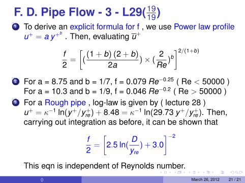
1 To derive an explicit formula for f , we use Power law profileu+ = a y+b . Then, evaluating u+

f2

=

[(

(1 + b) (2 + b)

2a)× (

2Re

)b]2/(1+b)

2 For a = 8.75 and b = 1/7, f = 0.079 Re−0.25 ( Re < 50000 )For a = 10.3 and b = 1/9, f = 0.046 Re−0.2 ( Re > 50000 )

3 For a Rough pipe , log-law is given by ( lecture 28 )u+ = κ−1 ln(y+/y+

re) + 8.48 = κ−1 ln(29.73 y+/y+re). Then,

carrying out integration as before, it can be shown that

f2

=

[2.5 ln(

Dyre

) + 3.0]−2

This eqn is independent of Reynolds number.() March 26, 2012 21 / 21