Mean Comparison: Manifest Variable versus Latent Variable∗

Ke-Hai Yuan

University of Notre Dame

and

Peter M. Bentler

University of California, Los Angeles

March 4, 2004

∗The research was supported by Grant DA01070 from the National Institute on Drug Abuse.

Abstract

Mean comparisons are of great importance in the application of statistics. Procedures for

mean comparison with manifest variables have been well studied. However, few rigorous stud-

ies have been conducted on mean comparisons with latent variables, although the methodol-

ogy has been widely used and documented. This paper studies the commonly used statistics

in latent variable mean modeling and compares them with parallel manifest variable statis-

tics in terms of power, asymptotic distributions, and empirical distributions. The robustness

property of each statistic is also explored when the model is misspecified or when data are

nonnormally distributed. Our results indicate that, under certain conditions, the likelihood

ratio and Wald statistics used for latent mean comparisons do not always have greater power

than the Hotelling T 2 statistics used for manifest mean comparisons. The noncentrality pa-

rameter corresponding to the T 2 statistic can be much greater than those corresponding to

the likelihood ratio and Wald statistics, which we find to be different from those provided in

the literature. Our results also indicate that the likelihood ratio statistic can be stochastically

much greater than the corresponding Wald statistic, and neither of their distributions can

be described by a chi-square distribution when the null hypothesis is not trivially violated.

Recommendations and advice are provided for the use of each statistic.

Keywords: Noncentrality parameter, likelihood ratio statistic, Wald statistic, empirical

power, parameter bias, asymptotic robustness.

1. Introduction

Comparing means of multiple variables is a central theme of many statistical proce-

dures. For example, ANOVA, MANOVA, growth curve modeling, etc., all aim to study

mean changes either across populations or across time. Because measurements in the social

and behavioral sciences are typically subject to errors, there has been a great interest in mean

comparisons of latent variables (LV) using the structural equation modeling (SEM) approach

(Bagozzi, 1977; Bagozzi & Yi, 1989; Bentler & Yuan, 2000; Byrne, Shavelson & Muthen,

1989; Cole, Maxwell, Arvey & Salas, 1993; Hancock, 2001, 2003; Hancock, Lawrence &

Nevitt, 2000; Kano, 2001; Kaplan & George, 1995; Kuhnel, 1988; McArdle & Epstein, 1987;

Meredith & Tisak, 1990; Muthen, 1989; Sorbom, 1974). When the observed variables are

subject to errors of measurement, modeling the means of LVs may be more meaningful sub-

stantively than a comparison of means of the observed or manifest variables (MV). However,

the LV approach cannot be applied to any set of variables. When a factor analysis model

does not hold for the observed data, it may be more appropriate to just evaluate means of

the MVs by using ANOVA or MANOVA (Cole, Maxwell, Arvey & Salas, 1993). Although

some research has been done on both the LV and MV approaches to mean comparisons, it is

not clear what statistical advantage the LV approach has over the MV approach, even under

idealized conditions. Our purpose is to compare these two approaches under ideal as well

as under more realistic conditions. The comparison includes a study of type I error, power,

parameter biases, and efficiency of parameter estimates.

The power of a mean comparison method is closely related to the effect size and sample

size, which affect the power through the so-called noncentrality parameter (NCP). Given the

sample size and effect size, one can figure out the corresponding NCP. With the NCP, one can

evaluate the overlap between the noncentral chi-square distribution (or F distribution) and

the corresponding central chi-square distribution (or F distribution), and further determine

power characteristics (see e.g., Hancock, Lawrence & Nevitt, 2000; Kaplan & George, 1995).

Such a comparison lies behind all the methods of power evaluations in the conventional

approaches to inference (e.g., Cohen, 1988; MacCallum, Browne & Sugawara, 1996; Satorra

& Saris, 1985). It is not an exaggeration to say that the NCP in the noncentral chi-square or

1

F distribution plays a key role in facilitating power comparisons. Actually, when the NCP

and degrees of freedom are known, the data, the sample size or the effect size are no longer

necessary in evaluating power. The NCP is easiest to obtain when comparing the means

of MVs. In the LV approach to mean comparisons, it is not clear how the NCP is related

to model misspecifications or effect sizes. In particular, it is not clear whether the NCP in

the LV approach equals that of the MV approach when testing, say, the population mean of

a multivariate normal distribution. A related issue is which approach is statistically more

powerful. When comparing the means of MVs, the statistic of choice is clear, for example,

the t or T 2. In the LV approach, there are the likelihood ratio (LR), Wald, and Lagrange

multiplier (LM) statistics (see chapter 10 of Bentler, 1995; Buse 1982; Satorra, 1989). Under

idealized conditions, these three procedures are asymptotically equivalent (see Engle, 1984).

In reality, they may not be equivalent, and thus it would be desirable to know which statistic

optimally controls type I errors and also achieves a nice power. We will discuss these issues

using analytical as well as Monte Carlo methods.

Kano (2001) thoroughly studied the effect of treating categorical group-indicator variables

as normally distributed in the SEM/LV approach to mean comparison. He also compared

power properties of MANOVA with that of SEM. Using asymptotics, he found that the

NCP in the SEM approach is the same as that in the MANOVA approach. Because there

are fewer degrees of freedom in the SEM approach, the power for finding mean differences

among latent variables is always greater than that in MANOVA. In his comparison, Kano

assumed that the factor loadings and unique variances are known. In practice, these are

seldom known in advance and have to be estimated from the data. It is not clear how the

NCP or power in the SEM approach is affected when the factor loadings and unique variances

are unknown. Hancock (2001) defined effect size and studied the power of mean comparisons

in the SEM approach. Using the normal theory based maximum likelihood, he determined

the relationships among power, NCP, and effect size. However, as we shall see, the NCP

given by Hancock also implicitly is based on the assumption that the factor loading matrix

is known, and thus the power and sample size determination procedures given by him are

limited to that situation. In section 2, we will provide a new formula for the NCP of several

2

models including the linear and nonlinear growth curves models. We also provide a general

result that characterizes the NCP in the LV and MV approaches to mean comparisons.

In the LV approach to a mean comparison, one commonly refers the LR or the Wald

statistic to a chi-square distribution, justified by asymptotics. Some regularity conditions

such as normally distributed data and large enough sample sizes have to be met. In section

3, we discuss these conditions and empirically study the behavior of several commonly used

statistics. We shall see that, even for normally distributed data, the commonly used statistics

cannot be even approximately described by chi-square distributions when the null hypothesis

is not trivially violated. In this situation, the Wald and LR statistics are not asymptotically

equivalent either.

When comparing means using the MV approach, conclusions will be biased if the co-

variance matrices in separate groups are assumed to be equal, but are actually not equal.

Similarly, in the LV approach, a misspecification in the covariance structure can affect the

evaluation of the mean structure. We will analytically characterize such effects in section 4,

and relate our results to those in the literature.

In practice, data may not be normally distributed. Commonly used procedures for mean

comparison, as implemented in standard software, are based on the normal distribution

assumption. In section 5, we will characterize the effect of nonnormality on several normal

theory based statistics. Under certain conditions, normal theory based procedures remain

asymptotically valid even when data are nonnormally distributed.

Both the MV and the LV approaches to mean comparison need regularity conditions. In

practice, both can be misused when applied blindly, without checking these conditions. A

related issue is how to minimize errors with a given procedure. In the concluding section, we

will summarize the problems with each method and discuss how to proceed when conditions

are not ideal.

2. NCP and Power Under Idealized Conditions

Let y1, y2, . . ., yn be a random sample from a p-variate normal distribution N(µ,Σ).

Assume that yi is generated by

yi = ν + Λξi + εi, (1a)

3

where ξi and εi are independent with E(ξi) = τ , Cov(ξi) = Φ, and Cov(εi) = Ψ is a

diagonal matrix. So the mean vector and covariance matrix of yi are

µ = ν + Λτ and Σ = ΛΦΛ′ + Ψ. (1b)

Using this structure for motivation, below we also study more general structures.

An interest in the MV approach is to test H01 : µ = 0. It is well-known that the Hotelling

T 2 is designed for such a purpose. It is given by

T 2 = ny′S−1y, (2)

where y is the sample mean and S is the sample covariance matrix. When using (2) to

test µ = 0, one usually transforms T 2 to an F statistic (see Anderson, 1984, p. 163). On

the other hand, the test statistics in the LV approach are justified by asymptotics. For the

purpose of comparing the LV and MV approaches, we will also describe the distribution of

T 2 by asymptotics (see also Kano, 2001). It is obvious that

T 2 L→ χ2p(δ1), (3a)

where

δ1 = nµ′Σ−1µ. (3b)

In the setup of model (1), testing µ = 0 can also be accomplished by testing some

more basic parameters in the mean structure. For example, when ν = 0 in (1b), µ = 0

is equivalent to τ = 0. More generally, suppose the elements of µ and Σ are further

parameterized as m(θ) and C(θ). When correctly specified, µ = m(θ0), Σ = C(θ0) and we

call θ0 the population value of θ. Let θ = (θ′1,θ′2)

′, where θ1 is a q1 × 1 vector containing

all the parameters that appear only in m(θ), and θ2 contains the q2 remaining parameters.

The normal theory based maximum likelihood estimator (MLE) θ of θ0 can be obtained by

minimizing (see Browne & Arminger, 1995)

FML(θ, y,S) = [y − m(θ)]′C−1(θ)[y −m(θ)] + tr[SC−1(θ)] − log |SC−1(θ)| − p. (4)

We need some notation for further technical development. For a p × p matrix A, let

vec(A) be the p2-dimensional vector formed by stacking the columns of A while vech(A) be

4

the p∗ = p(p+1)/2-dimensional vector formed by stacking the nonduplicated elements of A

leaving out the elements above the diagonal. There exists a unique p2 × p∗ matrix Dp such

that vec(A) = Dpvech(A) (Magnus & Neudecker, 1999). Let c = vech(C) and

W(θ) = 2−1D′p[C

−1(θ) ⊗C−1(θ)]Dp.

A dot on top of a function denotes a derivative, for example, m(θ) = dm(θ)/dθ. Partial

derivatives will be denoted by a subscript, for example m1(θ) = ∂m(θ)/∂θ1 and cλ(θ) =

∂c(θ)/∂λ. We often omit the argument of the function when it is evaluated at the population

value θ0. We will denote by 0p×q the matrix of dimension p× q whose elements are all 0, by

Ip the p × p identity matrix, and by 1p the vector of length p whose elements are all 1.0.

Suppose µ = m1θ01. Then testing for H01 : µ = 0 is equivalent to testing H02 : θ01 = 0.

We will mainly consider the Wald statistic in this section because the T 2 statistic in (2) and

the commonly used z statistic for evaluating the significance of a parameter estimate are also

Wald statistics. Under idealized conditions, the Wald statistic is asymptotically equivalent

to the LR and LM statistics (see Engle, 1984). In the context of SEM, the Wald statistic

for testing θ01 = 0 is given by

TW = θ′1[Acov(θ1)]

−1θ1, (5)

where Acov(θ1) is a consistent estimator of the asymptotic covariance matrix of θ1. Under

standard regularity conditions (see Satorra, 1989; Engle, 1984),

TWL→ χ2

q1(δ2), (6a)

where

δ2 = θ′01[Acov(θ1)]−1θ01. (6b)

We have the following theorem regarding the two NCPs δ1 and δ2.

Theorem 1. Suppose both m(θ) and C(θ) are correctly specified with µ = m1θ01. Then

δ1 = δ2 when m′1Σ

−1m2 = 0, and δ1 > δ2 otherwise.

Proof: Taking the second derivative of FML(θ, y,S) with respect to θ we obtain the

Hessian matrix whose expectation at θ0 is

−(m′Σ−1m + c′Wc).

5

Note that m = (m1, m2) and c = (0p∗×q1 , c2), which further give the information matrix for

minimizing (4) as

I =

(m′

1Σ−1m1 m′

1Σ−1m2

m′2Σ

−1m1 m′2Σ

−1m2 + c′2Wc2

). (7)

Let

A = I−1 =

(A11 A12

A21 A22

),

where A11 is of dimension q1 × q1 corresponding to θ1. Then

Acov(θ1) = A11/n = n−1[m′

1Σ−1m1 − m′

1Σ−1m2(m

′2Σ

−1m2 + c′2Wc2)−1m′

2Σ−1m1

]−1.

When m′1Σ

−1m2 = 0, Acov(θ1) = n−1(m′1Σ

−1m1)−1 and

δ2 = nθ′01m′1Σ

−1m1θ01 = nµ′Σ−1µ = δ1.

When m′1Σ

−1m2 6= 0, Acov(θ1) − n−1(m′1Σ

−1m1)−1 > 0, i.e., a positive definite matrix,

thus δ1 > δ2.

Of course, the hypothesis H02 can also be tested by LR statistics. Under the hypothesis

θ01 = 0, one can fix θ1 = 0 in (4) and just estimate θ2. Denote the estimator as θ2. Because

(m(θ2),C(θ2)) is nested within (m(θ),C(θ)), one LR statistic is

T(1)LR = n

[FML(θ2, y,S) − FML(θ, y,S)

].

In using the above LR statistic for testing θ01 = 0 one needs to make sure that m(θ) and C(θ)

are correctly specified. Otherwise, the power or type I error might not be properly controlled.

Of course, the saturated covariance model is automatically correct and (m(θ2),C(θ2)) is

nested within the saturated model. The LR statistic based on this nesting is

T(2)LR = nFML(θ2, y,S)

When (m(θ),C(θ)) is correctly specified and (m(θ2),C(θ2)) is not correctly specified, T(1)LR

and T(2)LR have the same NCP, but it is T

(1)LR that is asymptotically equivalent to the Wald

statistic TW in (5). Actually,

T(1)LR

L→ χ2q1

(δ2) and T(2)LR

L→ χ2p∗+p−q2(δ2).

6

Under idealized conditions, there also exists an LM statistic that is asymptotically equivalent

to TW and T(1)LR. However, the LM statistic is seldom used in mean comparisons, and thus

we will not explicitly deal with it here.

In the remainder of this section, we will study several important cases. We first consider

the simple one-group one-factor model so that enough details can be provided. We next

consider linear and nonlinear growth curve models that have two factors. A two-group one-

factor model will be considered at the end. By specializing to different cases, we will be able

to see the functional relationship of NCP with various model parameters.

2.1 One-group one-factor model

Consider the situation when ξi contains a single factor. Then Λ = λ is a vector and

we fix the variance of ξi = ξi at 1.0 to identify its scale. For simplicity, we further assume

that ν = 0, which also makes the mean structure identified. Thus, the mean and covariance

structures of (1) are

m(θ) = λτ, and C(θ) = λλ′ + Ψ, (8)

where θ1 = τ and θ2 = (λ′,ψ′)′ with ψ = (ψ11, ψ22, . . . , ψpp)′. It is easy to see that

m1 = λ, m2 = (τIp,0p×p), c2 = (cλ, cψ), and µ = m1θ01. (9)

Because m′1Σ

−1m2 6= 0, the NCP δ2 in (6b) for testing τ = 0 does not equal the NCP δ1 in

(3b). Using (7) and (9), we obtain the information matrix corresponding to model (8) as

I =

λ′Σ−1λ τλ′Σ−1 01×pτΣ−1λ τ 2Σ−1 + c′λWcλ c′λWcψ0p×1 c′ψWcλ c′ψWcψ

. (10)

The standard error of τ is given by√a11/n. Let

Q = Ip∗ − W1/2cψ(c′ψWcψ)

−1c′ψW1/2. (11)

By repeatedly using the formula of inversion for partitioned matrices (e.g., Magnus &

Neudecker, 1999, p. 11), we have

a11 =[λ′Σ−1λ− λ′Σ−1/2(Ip + τ−2Σ1/2c′λW

1/2QW1/2cλΣ1/2)−1Σ−1/2λ

]−1. (12)

7

The Wald test for τ = 0 is to refer tW =√nτ/

√a11 to the standard normal distribution

N(0, 1) or to use

TW = t2W = nτ 2a−111 ∼ χ2

1. (13)

When τ 6= 0, it follows from (12) and (13) that

TWL→ χ2

1(δ2), (14a)

where

δ2 = nτ 2a−111 = nµ′

[Σ−1 − Σ−1/2(Ip + τ−2Σ1/2c′λW

1/2QW1/2cλΣ1/2)−1Σ−1/2

]µ. (14b)

When λ and Ψ are known, Kano (2001) showed that the LR statistic for testing τ = 0 in

model (8) asymptotically follows χ21(δ1), where δ1 is given by (3b). Obviously, when λ and ψ

are known, m′1Σ

−1m2 = 0. When λ and Ψ are unknown, the NCP for inferring the means

of MVs is actually greater than the NCP corresponding to the LR statistic for inferring the

means of LVs. Actually, holding λ and Ψ constant, a−111 is a decreasing function of τ while

λ′Σ−1λ does not depend on τ . As τ increases, the difference between δ1 and δ2 gets larger.

Because T 2 is referred to χ2p(δ1) which has p−1 more degrees of freedom than χ2

1(δ2), δ1 > δ2

does not necessarily imply that inference for µ = 0 based on (3) is more powerful than that

based on (14). We are unable to give an analytical characterization of the magnitude of the

power difference between TW and T 2. A numerical comparison is used instead.

Let λ = (0.70, 0.70, 0.75, 0.75, 0.80, 0.80)′ and ψiis be chosen so that Σ is a correlation

matrix. At level α = 0.05, Table 1 provides the powers (β) of TW and T 2 when referring them

to χ21 and χ2

6 respectively, but their actual distributions are respectively χ21(δ2) and χ2

6(δ1).

Note that the sample size requirement for a statistic to be approximately described by its

asymptotic distribution is directly related to the degrees of freedom (see Yuan & Bentler,

1998). With 1 degree of freedom in TW and T(1)LR, n = 20 can be regarded as a small sample

size and n = 50 can be regarded as a medium sample size. For extra information, Table 1

also includes the powers of referring T(2)LR ∼ χ2

15(δ2) to χ215 and referring T 2 to the commonly

used F distribution through

TF = (n− p)T 2/{p(n − 1)} ∼ Fp,n−p. (15)

8

Notice that (15) is not a large sample approximation but the exact finite sample distribution

when data are normally distributed. At n = 20, TW is more powerful than T 2 and TF when

τ ≤ 1.0. T 2 is more powerful than TW when τ ≥ 1.2, and TF is also more powerful than TW

when τ ≥ 1.6. T(2)LR is the least powerful statistic due to its smaller NCP and the greater

degrees of freedom in its reference distribution. At n = 50, TW is more powerful than T 2

and TF until all of their powers reach essentially 1.0 at τ = 1.0. Notice that δ1 increases

much faster than δ2 as τ increases. Because T 2 has more degrees of freedom, its power is

not greater than TW until δ1 is much greater than δ2. Also notice that the powers of T 2, TW

and T(2)LR are based on large sample approximations which may not properly control type I

errors at smaller sample sizes. Actually, with normally distributed data, referring T 2 to χ26

for inference leads to greater type I errors than α = 0.05, as specified by the critical value.

Insert Table 1 about here

The statistic T 2 in (3a) for testing µ = 0 is based on a saturated model. One can also

formulate the problem of testing µ = 0 based on the estimated µ = τ λ from the structured

model with√n(µ− µ)

L→ N(0,V),

where V = Acov(√nµ) can be obtained from standard asymptotics (see Ferguson, 1996, p.

45). The corresponding test statistic is

TS = nµ′V−1µL→ χ2

p(δ1),

where δ1 is given by (3b). This indicates that µ = τ λ does not contain more information

about the underlying population parameter µ than y. Actually, each individual µj = τ λj is

more efficient than yj but different µjs also have greater correlations (overlapping informa-

tion) than those among the corresponding yjs.

Note that one can obtain estimates λ and ψ when modeling S by C(θ) without the

mean structure involved. The question is whether λ or ψ become more efficient by jointly

modeling the mean and covariance structures. It follows from (10) that the asymptotic

covariance matrix of√nλ is given by

Aλ ={[c′λWcλ − c′λWcψ(c

′ψWcψ)

−1c′ψWcλ] + τ 2[Σ−1 − Σ−1λ(λ′Σ−1λ)−1λ′Σ−1]}−1

9

and the asymptotic covariance matrix of√nψ is given by

Aψ ={σ′ψWcψ − c′ψWcλ

(c′λWcλ + τ 2[Σ−1 − Σ−1λ(λ′Σ−1λ)−1λ′Σ−1]

)−1c′λWcψ

}−1

.

The asymptotic covariance matrices of√nλ and

√nψ are respectively

Bλ =[c′λWcλ − c′λWcψ(c

′ψWcψ)

−1c′ψWcλ]−1

and

Bψ =[c′ψWcψ − c′ψWcλ(c

′λWcλ)

−1c′λWcψ]−1

.

Because

Σ−1 − Σ−1λ(λ′Σ−1λ)−1λ′Σ−1 ≥ 0,

we have

Aλ ≤ Bλ and Aψ ≤ Bψ.

The greater the τ the more efficient the estimator λ and ψ are. So both λ and ψ are more

efficient when jointly modeling the means and covariances. This is consistent with results

given by Yung and Bentler (1999).

A final note we’d like to make is that δ1 = µ′Σ−1µ = nτ 2(λ′Σ−1λ) is proportional

to the reliability of measurements in yi. Actually, λ′Σ−1λ = λ′Ψ−1λ/(1 + λ′Ψ−1λ) is

the maximum reliability of a weighted average of the p measurements (see Bentler, 1968;

Hancock & Mueller, 2001; Li, 1997; Raykov, 2004; Yuan & Bentler, 2002). For the given τ ,

the more reliable the measurements the greater the δ1 and δ2 are.

2.2 Growth curve model

Let yi = (yi1, yi2, . . . , yip)′ be repeated measures at p time points. Then a latent growth

curve model can be expressed by equation (1) (Meredith & Tisak, 1990; Curran, 2000;

Duncan, Duncan, et al., 1999), where ν = 0,

Λ =

(1 1 1 . . . 10 1 λ3 . . . λp

)′

, (16)

ξi = (ξi1, ξi2)′ with ξi1 being the latent slope and ξi2 being the latent intercept, τ = (τ1, τ2)

′,

Φ = Cov(ξi) =

(φ11 φ12

φ21 φ22

)

10

is the covariance matrix between the individual differences in intercept and slope. This setup

leads to the following mean and covariance structures

m(θ) = Λτ , C(θ) = ΛΦΛ′ + Ψ. (17)

When λ3 to λp in (16) are known constants, then model (17) represents a growth curve

model with predetermined or hypothesized growth rates. A special case is the initial value

linear growth model with λ3 = 2, λ4 = 3, . . ., λp = p− 1. With predetermined growth rates,

θ1 = (τ1, τ2)′ and θ2 = (φ′,ψ′)′, where φ = (φ11, φ21, φ22)

′. It is obvious that m1 = Λ and

µ = m1θ01. Because m2 = 0, m′1Σ

−1m2 = 0, the NCP δ2 in the asymptotic distribution of

the Wald statistic TW equals that in the asymptotic distribution of T 2. Since the likelihood

ratio statistic in the SEM approach has smaller degrees of freedom, it will have a greater

power than the T 2 statistic in testing µ = 0.

Actually, the normal theory based information matrix for model (17) with known λi is

I =

1′pΣ

−11p 1′pΣ

−1λ0 01×3 01×pλ′

0Σ−11p λ′

0Σ−1λ0 01×3 01×p

03×1 03×1 c′φWcφ c′φWcψ0p×1 0p×1 c′ψWcφ c′ψWcψ

, (18)

where λ0 = (0, 1, λ3, λ4, . . . , λp)′ is the prespecified vector of growth rates. Thus, A = I−1 =

diag(A11,A22) with A11 being the asymptotic covariance matrix of√nθ1 and A22 being the

asymptotic covariance matrix of√nθ2. So θ1 and θ2 are asymptotically independent. It also

follows from (18) that the MLEs of Φ and Ψ do not become more efficient when modeling

the mean and covariance structure simultaneously. This is because y does not contain any

information of the covariance parameters (φ,ψ).

When λ3 to λp in (16) are unknown, then (17) represents a growth curve model with an

arbitrary growth rate to be determined by (λj+1 − λj)τ2. In such a case, θ1 = τ = (τ1, τ2)′

and θ2 = (λ3, . . . , λp,φ′,ψ′)′. Let λ = (0, 1, λ3, . . . , λp)

′ and E = (e3, . . . , ep), where ei is

the ith unit vector in the Euclidean space. We have

m1 = Λ, and m2 = (τ2E,0p×(3+p)).

Consequently, µ = m1θ01 and m′1Σ

−1m2 6= 0. Thus, the NCP δ2 in (6b) for testing

θ01 = τ = 0 is smaller than the δ1 in (3b) for testing µ = 0.

11

The normal theory based information matrix for model (17) with unknown λj is

I =

1′pΣ

−11p 1′pΣ

−1λ τ21′pΣ

−1E 01×3 01×pλ′Σ−11p λ′Σ−1λ τ2λ

′Σ−1E 01×3 01×pτ2E

′Σ−11p τ2E′Σ−1λ τ 2

2E′Σ−1E + c′λWcλ c′λWcφ c′λWcψ

03×1 03×1 c′φWcλ c′φWcφ c′φWcψ0p×1 0p×1 c′ψWcλ c′ψWcφ c′ψWcψ

. (19)

It follows from (19) that the asymptotic covariance matrix of√nτ is

A11 =

{(1′p

λ′

) [Σ−1 − (Σ−1E)(E′Σ−1E)−1/2M(E′Σ−1E)−1/2(E′Σ−1)

] (1p λ

)}−1

,

where

M ={Ip−2 + τ−2

2 (E′Σ−1E)−1/2c′λW1/2HW1/2cλ(E

′Σ−1E)−1/2}−1

with

H = Ip∗ − W1/2(

cφ cψ) [( c′φ

c′ψ

)W

(cφ cψ

)]−1 (c′φc′ψ

)W1/2.

Thus,

δ2 = nµ′Σ−1µ− nµ′Σ−1E(E′Σ−1E)−1/2M(E′Σ−1E)−1/2E′Σ−1µ.

Notice that M is a function of τ2 but not of τ1. When τ2 increases, δ2 increases not as fast

as δ1. So, once again, the LR or the Wald statistic will have a greater power than T 2 for

smaller τ2 and the opposite is true for larger τ2. Also notice that, when τ2 = 0, m2 = 0 and

consequently δ2 = δ1. Then the likelihood ratio statistic or TW will always have a greater

power than T 2 regardless of how large τ1 is.

2.3 Two-group one-factor model

Suppose x1, x2, . . ., xn1 ∼ N(µ1,Σ1) and y1, y2, . . ., yn2 ∼ N(µ2,Σ2) are two indepen-

dent random samples. We further assume that both the samples are generated by one-factor

models and µ1, µ2, Σ1, Σ2 can be correctly modeled by

m1(θ) = ν, m2(θ) = ν + λτ, C1(θ) = C2(θ) = λλ′ + Ψ, (20)

where θ = (τ,ν ′,λ′,ψ′). Although the setup does not fall into the category of Theorem 1,

the results that are going to be obtained for T 2 and TW are closely related to the one-group

case considered in subsection 2.1.

12

Using the MV approach, one can test H03 : µ1 = µ2 by

T 2 =n1n2

N(y − x)′S−1(y − x), (21)

where S is the pooled sample covariance matrix and N = n1 + n2. When µ1 6= µ2,

T 2 L→ χ2p(δ3) (22a)

as n1 and n2 increase, where

δ3 = Nr1r2τ2λ′Σ−1λ = Nr1r2(µ2 − µ1)

′Σ−1(µ2 − µ1), (22b)

with r1 = n1/N and r2 = n2/N .

The interest in the LV approach is to test H04 : τ = 0, which is equivalent to testing

µ1 = µ2 in the setup of (20). The MLE θ of θ can be obtained by minimizing

FML(θ, x,S1, y,S2) = r1FML(θ, x,S1) + r2FML(θ, y,S2). (23)

The information matrix associated with minimizing (23) is

I =

r2λ′Σ−1λ r2λ

′Σ−1 r2τλ′Σ−1 01×p

r2Σ−1λ Σ−1 r2τΣ

−1 0p×pr2τΣ

−1λ r2τΣ−1 r2τ

2Σ−1 + c′λWcλ c′λWcψ0p×1 0p×p c′ψWcλ c′ψWcψ

. (24)

When both n1 and n2 increase, standard asymptotics imply that

√N (θ − θ0)

L→ N(0,I−1). (25)

Denote A = (aij) = I−1. Then

a11 = (r1r2)−1{λ′Σ−1λ − λ′Σ−1/2

[Ip + (r1r2τ

2)−1Σ1/2c′λW1/2QW1/2cλΣ

1/2]−1

Σ−1/2λ}−1

,

(26)

where Q is given in (11). The Wald statistic for testing τ = 0 is

TW = Nτ 2a−111 . (27)

When τ 6= 0,

TWL→ χ2

1(δ4), (28a)

13

where

δ4 = Nτ 2a−111 = Nr1r2(µ2 − µ1)

′P(µ2 − µ1) (28b)

with

P = Σ−1 −Σ−1/2[Ip + (r1r2τ

2)−1Σ1/2c′λW1/2QW1/2cλΣ

1/2]−1

Σ−1/2.

Comparing (28b) with (22b), δ4 ≤ δ3 and the inequality is strict when τ 6= 0. Notice

that, when holding λ and ψ constant,

λ′Σ−1/2[Ip + (r1r2τ

2)−1Σ1/2c′λW1/2QW1/2cλΣ

1/2]−1

Σ−1/2λ

is an increasing function of r1r2τ2. Thus, δ3 − δ4 increases as r1r2τ

2 increases. Comparing

(22b) with (3b) and (28b) with (14b), we find that the difference between LV and MV

approaches to mean comparison in the two-group case is almost the same as in the one-

group case. Actually, when changing r1r2τ2 to τ 2 and N to n, the result in the two-group

case turns to that in the one-group case. Based on the numerical result of the one-group

case, the power of TW based on (28) will be greater than that based on (22) for smaller τ ,

while the opposite is true for larger τ .

When λ and ψ are known, Kano (2001) obtained the same NCP for both the LV and

MV approaches to mean comparison as that given in (22). Hancock’s (2001) formula for the

NCP of the likelihood ratio statistic is just (22b) in the setup of model (20). This equals

(28b) only when λ is known or m(θ) satisfies m′1Σ

−1m2 = 0. Under a sequence of local

alternatives (see Stroud, 1972), it can be shown that the likelihood ratio statistic for testing

τ = 0 in model (20) also asymptotically follows the chi-square distribution as specified in

(28).

3. Empirical Behaviors of the Statistics with Normally Distributed Data and Fixed

Alternative Hypothesis

The previous section showed that the T 2 statistic in the MV approach and the Wald

statistic in the LV approach to mean comparison do not have the same NCP unless the

mean structure satisfies certain conditions as in the linear growth curve model. Under

idealized conditions, the LR statistic is asymptotically equivalent to the Wald statistic, so

14

the LR statistic T(1)LR does not have the same NCP as that of the T 2 statistic. In this section,

we will study the behavior of the LR statistics, the Wald statistic and the T 2 statistic when

conditions are not ideal. Specifically, with normally distributed data we will consider a fixed

alternative hypothesis rather than a sequence of local (or contiguous) alternative hypotheses.

The sample size will be small or medium instead of huge. A Monte Carlo study comparing

the LM, the Wald and the LR statistics in the context of only covariance structure analysis

was conducted by Chou and Bentler (1990). Our analysis and result below will provide more

insight to the three statistics in mean and covariance structure models.

3.1 Alternative hypothesis and theoretical NCP

Let (µn,Σn) be a sequence of alternative hypotheses and θ∗ satisfy

minθFML(θ,µn,Σn) = FML(θ

∗,µn,Σn).

In order to establish that the LR or the Wald statistic asymptotically follows a noncentral

chi-square distribution one needs to assume

µn = m(θ∗) + δ/√n, Σn = C(θ∗) + ∆/

√n, (29)

where δ is a p-dimensional vector and ∆ is a p × p matrix, and neither depends on n.

Notice that the m(θ) in (29) is correctly specified for modeling µn when δ = 0 and C(θ)

is correctly specified for modeling Σn when ∆ = 0. The amount of misspecification in (29)

decreases as n increases with limn→∞µn = µ(θ∗) and limn→∞Σn = C(θ∗). When µn and

Σn represent the population under consideration and θ0 is the population value of θ that

corresponds to a correct model structure, under (29) θ is consistent for θ0, that is θ∗ = θ0.

Let ϕ = nFML(θ∗,µn,Σn). Under (29), one can further show that (see e.g., Satorra, 1989;

Steiger, Shapiro & Browne, 1985)

δ2 ≈ ϕ (30)

and (30) becomes exact when n = ∞.

However, when fitting (m(θ),C(θ)) to (y,S), the alternative hypothesis is µn = E(y) =

µ and Σn = E(S) = Σ, which do not depend on n. In such a realistic situation, θ∗ will

not equal θ0; (30) may not hold; the Wald statistic TW and the LR statistic T(1)LR may

15

not be asymptotically equivalent either. Actually, condition (29) is just a mathematical

convenience; without it, one cannot show, for complicated models as in the context of SEM,

that the LR statistic asymptotically follows a noncentral chi-square distribution. We have

to use numerical procedures to study the difference between δ2 and ϕ and simulation to

illustrate the discrepancy between the statistic T(1)LR and the chi-square distribution with

NCP ϕ. In the simulation we also study the statistics T 2, TW , T(1)LR, T

(2)LR.

Insert Table 2 about here

Using the same model as for producing the result of Table 1, the NCP ϕ and the powers

of referring T(1)LR to χ2

1 and T(2)LR to χ2

15 are reported in Table 2, where the real distributions

are T(2)LR ∼ χ2

1(ϕ) and T(2)LR ∼ χ2

15(ϕ). For comparison purpose, δ2 and the powers of TW

and T(2)LR from Table 1 are also copied here. It is easy to see that ϕ > δ2 for all the τ s in

Table 2. Consequently, TW and T(1)LR are no longer equivalent. Actually, the corresponding

power of T(1)LR is greater than that of TW due to ϕ > δ2. Based on our numerical exploration

with different factor loadings, error variances, and τ s with model (1), we predict that ϕ is

always greater than δ2 when τ 6= 0. But we are unable to provide an analytical answer.

Our exploration also indicates that, when holding all the other parameters constant, the

magnitude of ϕ − δ2 is an increasing function of τ . When τ is tiny, ϕ ≈ δ2, which is

also implicitly implied by the ideal condition specified in (29). When n is near ∞, the

misspecification δ/√n in (29) will be tiny, and TW and T

(1)LR having the same power implies

that ϕ = δ2.

Comparing Tables 1 and 2, we may observe that T 2 ∼ χ2p(δ1) is still more powerful than

T(1)LR ∼ χ2

1(ϕ) when τ ≥ 1.2. Another observation is that ϕ is still much smaller than δ1 when

τ is large, although it is greater than δ2.

3.2 Empirical power

The distributions of the statistics that generated the powers in Tables 1 and 2 are based

on asymptotics. With finite sample sizes and fixed alternative hypotheses, it is not clear how

well the behavior of the statistics can be described by chi-square distributions. To better

understand these statistics, a simulation is performed with normally distributed data. The

16

model and parameters are the same as those that produced Tables 1 and 2. With n = 20, 50,

Table 3 contains empirical powers, β, of TF , T 2, TW , T(1)LR and T

(2)LR, where 95th percentiles of

the corresponding asymptotic null distributions are used in judging the significance of each

statistic over 500 replications.

Insert Table 3 about here

The first line in Table 3 contains the power or type I error when τ = 0 and n = 20.

When the model is correct, the ideal situation is to have a 5% rejection. Both T 2 and

T(2)LR over-reject the correct model, implying that their behavior cannot be well described by

their asymptotic distributions. On the other hand, type I errors of TF , TW and T(1)LR are

approximately at 5%. Notice that the statistic TF is referred to an exact distribution, thus,

the discrepancy between β(TF ) and β(TF ) is just due to sampling errors. As τ increases,

the powers by all the statistics increase while those of TW and T(1)LR increase the fastest.

According to the asymptotic results in Tables 1 and 2, T 2 has a greater power than TW or

T(1)LR when τ = 1.2, but TW has a greater empirical power in Table 3. The statistic T

(1)LR

always has a greater power than TW according to Table 2, however, their empirical powers

are about the same in Table 3. The bottom panel of Table 3 contains the powers when

n = 50. As sample size increases, type I errors of T 2 and T(2)LR are more near the nominal

level of 0.05. Comparing Table 3 with Tables 1 and 2 we may also observe that, except for

the statistic TF , the empirical powers for the other four statistics are always greater than

the corresponding asymptotic powers.

3.3 Empirical NCP

An interesting phenomenon is that in Table 2, β(T(1)LR) > β(TW ), while the difference

between β(TW ) and β(T(1)LR) is smaller than that between β(TF ) and β(TF ). Because β(TF )−

β(TF ) is just sampling error, β(TW ) and β(T(1)LR) might be regarded as essentially equal. The

discrepancy between β and β corresponding to TW and T(1)LR deserves further understanding.

For such a purpose, we first obtain the empirical NCPs corresponding to TW and T(1)LR and

see how much they differ.

Insert Table 4 about here

17

Let TWi be the statistic TW evaluated at the ith replication, δ2i = TWi − 1 and

δ2 =1

500

500∑

i=1

δ2i.

Both statistics T(1)LR and T

(2)LR asymptotically follow chi-square distributions with the same

NCP ϕ. Their estimates can be obtained by ϕ1 = T(1)LR − 1 and ϕ2 = T

(2)LR − 15. The average

estimators over 500 replications are ϕ1 and ϕ2, respectively. Similarly, two estimators for

δ1 are obtained using TF ∼ Fp,n−p(δ1) and T 2 ∼ χ2p(δ1). The average estimators over 500

replications are δ11 and δ12, respectively. Notice that E(δ11) = δ1 for all the τ s and ns. So we

may regard δ11 − δ1 as a sampling error. It is obvious from Table 4 that δ12 over-estimates

δ1 and the amount of over-estimation increases as δ1 increases and decreases as n increases.

The estimation of δ2 by δ2 is quite good overall. However, at n = 20, δ2 over-estimates δ2

when δ2 = 0, 0.2 and δ2 under-estimates δ2 when δ2 = 0.4 to 2.0. A similar pattern also exists

when n = 50. This may imply that the discrepancy between TW and χ21(δ2) systematically

changes as δ2 increases. The estimator ϕ2 consistently over-estimates ϕ. The amount of

over-estimation is pretty much the same as ϕ increases, and decreases when n increases. As

an estimator of ϕ, ϕ1 is pretty good and there does not seem to exist a systematic pattern

of bias at n = 20. When n = 50 and τ ≥ 0.8, ϕ1 is consistently smaller than ϕ. This may

imply that the discrepancy between T(1)LR and χ2

1(ϕ) systematically changes as τ increases.

Although β(TW ) and β(T(1)LR) are about the same, ϕ1 is always greater than δ2. This implies

that there exists a systematic difference in distribution shapes of TW and T(1)LR.

3.4 Empirical distribution

We next use quantile-quantile (QQ) plots to better understand the distributions of the

statistics. We will study the distributions of TF , T 2, TW , T(1)LR and T

(2)LR. For each statis-

tic, eleven QQ plots corresponding to τ = 0, 0.2 . . ., 2.0 were created. To save space we

only present the QQ plots when τ = 0, 0.2, 1.0 and 1.8. These four plots give us enough

information about the distribution change of each statistic as τ and n change.

Insert Figure 1 about here

Figures 1(a) and (b) contain the plots of the statistic TF against the distribution Fp,n−p(δ1)

when n = 25 and 50, respectively. Notice that the distribution Fp,n−p(δ1) exactly describes

18

the behavior of TF . In Figure 1, the quantiles of TF match those of Fp,n−p(δ1) very well from

left tail to approximately the median; however, they do not match well from approximately

the median to the right tail. As n increases, the discrepancy between the two sets of quantiles

becomes smaller. But there is no systematic pattern in the discrepancy when τ changes. This

is probably because the discrepancy is totally due to sampling errors.

Insert Figure 2 about here

Figures 2(a) and (b) contain the plots of the quantiles of T 2 against those of χ2p(δ1). It

is obvious that essentially all the quantiles of T 2 are above those of the corresponding ones

of χ2p(δ1) when n = 20, only those near the very left tail are close. The right tail of T 2 is

way above that of χ2p(δ1). When n = 50, T 2 is better described by χ2

p(δ1). The majority of

the quantiles of T 2 are still above the corresponding ones of χ2p(δ1) when τ is small. As τ

increases, the left tail of T 2 is shorter than that of χ2p(δ1) while the right tail of T 2 is much

longer than that of χ2p(δ1).

Insert Figure 3 about here

Figures 3(a) and (b) contain the QQ plots of TW against those of χ21(δ2). At τ = 0, the

distribution of TW can be described by χ21 quite well when compared to Figure 1. However,

the distribution of TW gradually departs from χ21(δ2) as τ or δ2 increases. When τ = 1.8,

TW has a much longer tail on the left and a much shorter tail on the right. The sample size

n has little effect in controlling the discrepancy between TW and χ21(δ2).

Insert Figure 4 about here

Figures 4(a) and (b) contain the QQ plots of T(1)LR against those of χ2

1(ϕ). The distribution

of T(1)LR can be described by χ2

1(ϕ) quite well when τ or ϕ is small. However, the distribution

of T(1)LR gradually departs from χ2

1(ϕ) as τ increases. When τ = 1.8, T(1)LR has a much longer

tail on the left and a much shorter tail on the right. The sample size n has little effect

in controlling the discrepancy between T(1)LR and χ2

1(ϕ). Comparing Figures 3 and 4, the

discrepancy between T(1)LR and χ2

1(ϕ) is a lot smaller than that between TW and χ21(δ2).

19

Insert Figure 5 about here

Statistics T(1)LR and TW are asymptotically equivalent under idealized conditions. With

a fixed alternative, neither of them can be described well by their asymptotic distributions

even for normally distributed data. It is interesting to see how different they are empirically.

Figures 5(a) and (b) compare the quantiles of T(1)LR against those of TW . When τ = 0, the

two statistics follow approximately the same distribution even at n = 20 and essentially

identical distribution at n = 50. As τ increases, they depart first at the right tail and then

the whole range. At τ = 1.8, TW is stochastically much smaller than T(1)LR. This discrepancy

is proportional to sample size n.

Insert Figure 6 about here

Figures 6(a) and (b) plot the quantiles of T(2)LR against those of χ2

15(ϕ). At n = 20 and

τ = 0, the quantiles near the left tail of T(2)LR approximate those of χ2

15(ϕ) reasonably well,

but T(2)LR has a longer right tail. As τ increases, the right tail of T

(2)LR becomes shorter than

that of χ215(ϕ), the left tail becomes longer. At n = 50, the overall distribution of T

(2)LR is

better approximated by χ215(ϕ) when τ is small. But, as τ increases, the left tail of T

(2)LR

becomes longer while the right tail becomes shorter than those of χ215(ϕ).

Figures 1 to 6 imply that, except for the statistic TF , no statistic can be well approximated

by its target or asymptotic distribution. One can show that, as n → ∞, the distribution of

T 2 can be closely described by χ2p(δ1) regardless of δ1. However, for the statistics TW , T

(1)LR

and T(2)LR, large sample size alone cannot guarantee that their distributions are approximately

chi-squares. Actually, the alternative hypothesis τ is more critical than the sample size n in

describing the distributions of the statistics TW , T(1)LR and T

(2)LR. When τ is small, the behavior

of TW and T(1)LR can be described by their asymptotic distributions pretty well even when n

is small. When τ is large, a larger n does not make TW , T(1)LR and T

(2)LR better approximated

by their asymptotic distributions. But a larger n does make them better described by their

asymptotic distributions when τ = 0.

The figures also provide additional information regarding the empirical powers and NCPs

reported in Tables 3 and 4. Because most of the quantiles of T 2 are above the corresponding

20

ones of χ2p(δ1), β(T 2) > β(T 2) and δ12 > δ1. The discrepancy will gradually disappear when

n → ∞. As τ increases, the quantiles from the median to the right tail of TW become

increasingly smaller than the corresponding ones of χ21(δ2). Although the lower quantiles of

TW also become greater than the corresponding ones of χ21(δ2), the extent of the greatness

is not as large as that of the smallness. Thus, δ2 < δ2 for larger τ . Notice that the empirical

power β(TW ) is evaluated by comparing each TWi to the critical value (χ21)

−1(0.95) ≈ 3.841.

The quantiles of TW around 3.841 are greater than those of χ21(δ2). Although the upper tail

of TW are shorter than that of χ21(δ2), it does not make any difference as long as it is above

(χ21)

−1(0.95). This also explains why β(TW ) > β(TW ). Due to essentially the same reason,

β(T(1)LR) > β(T

(1)LR) and ϕ1 < ϕ for larger τ . It is obvious from the QQ plots in Figure 5

that the quantiles of TW match those of T(1)LR very well around the critical value (χ2

1)−1(0.95),

but those of TW are much smaller than the corresponding ones of T(1)LR at the upper tails,

especially for larger τ . This explains why β(TW ) and β(T(1)LR) are about the same while

ϕ1 > δ2. Similarly, because the quantiles of T(2)LR around (χ2

15)−1(0.95) ≈ 24.996 are greater

than those of χ215(ϕ), β(T

(2)LR) > β(T

(2)LR), and ϕ2 > ϕ when majority of the quantiles of T

(2)LR

are greater than the corresponding ones of χ215(ϕ).

A final note we would like to make is that the empirical performance of TW , T(1)LR and T

(2)LR

under alternative hypotheses obtained in this section might be different from that reported

in Chou and Bentler (1990) and Curran et al. (2002). Without a mean structure, Chou

and Bentler as well as Curran et al studied the commonly used statistics with misspecified

covariance structures. Our results hold for a misspecified mean structure with a correctly

specified covariance structure. All 500 replications in all the conditions reported in Figures

1 to 6 converged while Curran et al.’s conclusion was based on a converged subset of a larger

number of replications.

4. Parameter Biases due to Model Misspecifications

In this section we develop some analytical results regarding the effect of misspecified

models on parameters. Yuan, Marshall and Bentler (2003) studied the effect of a misspecified

model on parameter estimates in the context of covariance structure analysis. This section

21

generalizes their result to mean structures. Specifically, parameters will be biased when the

model is misspecified. The bias makes the LR test and the z or Wald test on parameter

values inaccurate. We also relate the analytical results obtained here to empirical findings

reported in the literature.

In the context of MANOVA, the µ and Σ are saturated. The parameter estimates µ = y

and Σ = S are unbiased. A possible bias in estimating the covariance matrix can be due to

the misspecification of a common Σ when separate groups have different variance-covariance

matrices. Using the setup of subsection 2.3, the true population covariance matrix of y − x

is

Cov(y − x) =1

n1Σ1 +

1

n2Σ2.

When assuming a common covariance matrix, the estimator of Cov(y− x) in the T 2 statistic

in (21) is

Cov(y − x) =N

(N − 2)n1n2[(n1 − 1)S1 + (n2 − 1)S2].

When Σ1 6= Σ2, the bias is

B = E[Cov(y − x)]− Cov(y − x) =(N − 1)(n2 − n1)

(N − 2)n1n2(Σ2 − Σ1).

This bias will affect the performance of the statistics TF and T 2.

Without loss of generality, let us consider n2 > n1. When Σ2 − Σ1 > 0, B > 0. Let

T 2c be the corresponding Hotelling’s statistic when Σ1 = Σ2. Then E(T 2) < E(T 2

c ) and

T 2 is stochastically smaller than T 2c . Similarly, when Σ2 < Σ1, E(T 2) > E(T 2

c ) and T 2 is

stochastically greater than T 2c . This explains why the type I errors of TF is smaller than the

nominal error when n2 > n1 and Σ2 > Σ1, as has been reported in simulation studies on TF

by Algina and Oshima (1990) and Hakstian, Roed and Lind (1979). More elaborate studies

on T 2 using asymptotics can be found in Ito and Schull (1964).

Yuan, Marshall and Bentler (2003) studied the bias in θ caused by a misspecified C(θ)

in covariance structure analysis only. In the context of SEM, both m(θ) and C(θ) can be

misspecified. Let m∗(υ) and C∗(υ) be the correct mean and covariance structures, thus

there exists a vector υ0 such that µ = m∗(υ0) and Σ = C∗(υ0). Let the misspecified

models be m(θ) and C(θ). We assume that the misspecification is due to m(θ) and C(θ)

22

missing parameters ϑ of υ = (θ′,ϑ′)′. Under standard regularity conditions (e.g., Kano,

1986; Shapiro, 1984), θ converges to θ∗ which minimizes FML(θ,µ,Σ). Note that in general

θ∗ does not equal its counterpart θ0 in υ0 = (θ′0,ϑ′0)

′, which is the population value of the

correctly specified models. We will call ∆θ = θ∗ − θ0 the bias in θ∗, which is also the

asymptotic bias in θ. It is obvious that, if the sample is generated by µ0 = m(θ0) and

Σ0 = C(θ0), then θ∗ will have no bias. We may regard the true population (µ,Σ) as a

perturbation to (µ0,Σ0). Due to the perturbation, θ∗ 6= θ0, although some parameters in

θ∗ can still equal the corresponding ones in θ0 (see Yuan et al., 2003).

It is obvious that θ0 minimizes FML(θ,µ0,Σ0), under standard regularity conditions, θ0

satisfies the normal equation h(θ0,µ0,σ0) = 0, where

h(θ,µ,σ) = m′(θ)C−1(θ)[µ−m(θ)]+ c′(θ)W(θ){σ+vech[(µ−m(θ))(µ−m(θ))′]−c(θ)}.

Because

h−1θ (θ0,µ

0,σ0) = −(m′C−1m + c′Wc)

is invertible, under standard regularity conditions (see Rudin, 1976, pp. 224-225), equation

h(θ,µ,σ) = 0

defines θ as an implicit function of µ and σ in a neighborhood of (µ0,σ0). Denote this

function as θ = f(µ,σ), then it is continuously differentiable in the neighborhood of (µ0,σ0)

with

f(µ0,σ0) = (m′C−1m + c′Wc)−1(m′C−1 c′W

). (31)

It follows from (31) that the perturbation (∆µ,∆σ) causes a perturbation in θ approximately

equal to

∆θ ≈ (m′C−1m + c′Wc)−1(m′C−1∆µ+ c′W∆σ). (32)

In the context of only a covariance structure model, ∆µ = 0, Yuan et al. (2003) for-

mulated the perturbation ∆σ further as a function of the omitted parameters in C(θ), for

example, the covariances among errors in a factor model. Equation (32) extends the result

of Yuan et al. (2003) to mean structures as well as to any perturbations ∆µ = µ − µ0 and

∆σ = σ−σ0. So the bias in θ∗ caused by the perturbation of misspecifications in m(θ) and

23

c(θ) is approximately given by the ∆θ in (32). Equation (32) implies that the bias in θ∗

caused by ∆µ and ∆σ are approximately additive. Let q be the number of free parameters

in θ. The coefficients of ∆σ in bias ∆θ are contained in the q × p∗ matrix

(m′C−1m + c′Wc)−1c′W.

For example, the lth row (cl,11, . . . , cl,p1; cl,22, . . . , cl,p2; . . . ; cl,pp) of the matrix are the coeffi-

cients for

(∆σ11, . . . ,∆σp1;∆σ22, . . . ,∆σp2; . . . ;∆σpp)

corresponding to the lth parameter in θ. When cl,ij = 0, the perturbation ∆σij has no effect

on θl. Similarly, the coefficients of ∆µ in ∆θ are contained in the q × p matrix

(m′C−1m + c′Wc)−1m′C−1.

To better understand equation (32) we next consider a misspecified covariance structure on

a mean parameter.

Suppose the population mean vector µ and covariance matrix Σ are generated by

µ = τλ1 and Σ = ΛΛ + Ψ,

where λ1 = (λ′11,λ

′21)

′ and

Λ =

(λ11 λ12 0λ21 0 λ23

).

Let µ0 = µ and Σ0 = λ1λ′1 + Ψ. It is obvious that model (1) with ν = 0 represents correct

mean and covariance structures for (µ0,Σ0). The misspecification in (1) for (µ,Σ) is in the

covariance structure C(θ) not in the mean structure m(θ). The perturbation is

∆σ = vech

(λ12λ

′12 0

0 λ23λ′23

).

With θ = (τ,λ′,ψ′)′, the bias in τ due to the omitted factors in the factor model is approx-

imately given by the first number in the vector

(m′C−1m + c′Wc)−1c′Wvech

(λ12λ

′12 0

0 λ23λ′23

).

This bias is proportional to λ12 and λ23.

24

In special cases, we can get the exact bias instead of the approximate one given in (32).

Let’s consider the situation that the population mean vector µ and population covariance

matrix Σ are generated by model (1) with ν = 0, Λ = λ being a vector. However, one

assumes τ = 0 in the model. Then m = 0 and θ = (λ′,ψ′)′. The value of θ∗ is obtained by

minimizing FML(θ,µ,Σ). The corresponding score function (gradient) is

g(θ) = c′(θ)W(θ)[vech(µµ′ + Σ) − c(θ)],

where

µµ′ + Σ = τ 2λλ′ + λλ′ + Ψ = (1 + τ 2)λλ′ + Ψ.

It is obvious that

λ∗ = λ√

1 + τ 2 and ψ∗ = ψ

satisfy g(θ∗) = 0. So the bias in λ∗ is (√

1 + τ 2 − 1)λ.

Parallel to (32), in the two-group mean comparison, as in section 2.3, the θ∗ that min-

imizes FML(θ,µ1,Σ1,µ2,Σ2) also contains biases. With perturbations ∆µ1 = µ1 − µ01,

∆σ1 = σ1 − σ01, ∆µ2 = µ2 − µ0

2, ∆σ2 = σ2 − σ02, the bias is approximately

∆θ ≈ L−1[r1m′1C

−11 ∆µ1 + r1c

′1W1∆σ1 + r2m

′2C

−12 ∆µ2 + r2c

′2W2∆σ2],

where

L = r1m′1C

−11 m1 + r1c

′1W1c1 + r2m

′2C

−12 m2 + r2c

′2W2c2.

There are conditions under which misspecifications in the covariance matrix do not affect

the mean parameters at all. Using the setup of Theorem 1, when m′1C

−1m2 = 0, there exist

(m′C−1m + c′Wc)−1 =

((m′

1C−1m1)

−1 00 (m′

2C−1m2 + c′2Wc2)

−1

),

m′C−1 =

(m′

1C−1

m′2C

−1

), c′W =

(0

c′2W

).

Thus,

∆θ =

(∆θ1

∆θ2

)=

((m′

1C−1m1)

−1m′1C

−1∆µ(m′

2C−1m2 + c′2Wc2)

−1(c′2W∆σ + m′2C

−1∆µ)

).

So the perturbations in ∆σ do not contribute to ∆θ1, which contains all the mean param-

eters. A special case of it is the growth curve model (17) with predetermined growth rates,

25

a misspecified C(θ) does not affect the τ1 and τ2. There are other special cases in which

misspecified C(θ) do not interfere with the estimation of mean parameters. When µ = 0 in

the one-group factor model considered in section 2.1, τ ∗ = 0 whether C(θ) is misspecified or

not. When µ = 0 in the nonlinear growth curve model, τ ∗1 = τ ∗2 = 0 even when C(θ) is mis-

specified. Similarly, when µ1 = µ2 in the two-group factor model considered in subsection

2.3, τ ∗ = 0 even when C(θ) is misspecified. These conclusions can be obtained by directly

inspecting the FML function.

Insert Table 5 about here

Let us next consider the effect of a misspecified covariance structure on the NCPs for the

test statistics TW , T(1)LR and T

(2)LR, using a numerical example. For comparison purposes, the

same model as generating Tables 1 to 4 is used here. Let (µ0,Σ0) be the same as specified

in generating previous Tables. When σ34, σ45 and σ56 are perturbed simultaneously by 0.2,

formula (32) gives the approximated bias on τ ∗ as ∆τ = 0.2(c1,34 + c1,45 + c1,56). We also

evaluated the true bias ∆∗τ = τ ∗− τ0. The second and third columns of numbers in Table 5

show that formula (32) approximates the true bias quite well. As τ increases, the bias also

increases. Notice that the biases are obtained using the population parameters and are not

affected by sample size n. When Σ is perturbed, the asymptotic NCP in the Wald statistic

is affected. When τ ∗ becomes smaller due to the bias, the corresponding NCP δ∗2 should be

smaller than the corresponding NCP δ2 that without the perturbation. However, δ∗2 > δ2

when τ ≥ 1.6. This can be seen from equation (14b) that δ2 does not necessarily increase as

τ increases while Σ changes. The NCP ϕ∗1 corresponding to T

(1)ML also decreases when C(θ)

is misspecified. Unlike δ2, ϕ∗1 monotonically increases as τ increases, so does (ϕ∗

1 − ϕ). The

last column of numbers in Table 5 are the NCP ϕ∗2 corresponding to T

(2)ML, which tests both

the mean and covariance structures simultaneously. The significance of T(2)ML can be due to

a misspecified m(θ) or a misspecified C(θ). Although T(1)ML may not correctly reflect the

magnitude of τ with a misspecified C(θ), it is much more reliable than T(2)ML. This is quite

different from the results in Yuan and Bentler (in press), where a misspecified Ca(θ) can

have a much greater effect on the nested chi-square test when used to test a further restricted

Cb(θ). Several numerical examples illustrating different aspects of misspecified covariance

26

structures on mean parameters are also provided in Yuan and Bentler (in press). For example,

they showed that a misspecified mean structure m(θ) have a much more dramatic effect on

the mean parameters than a misspecified covariance structure, and a misspecified Ca(θ)

make the nested chi-square test totally unreliable when testing the structure of Cb(θ).

With a misspecified C(θ), we should not expect any of the statistics to empirically behave

better than when C(θ) is correctly specified.

5. Distribution Violations

In previous sections we studied mean inference for normally distributed data. In practice

data may not be normally distributed. In this section, we study the effect of nonnormal data

on the test statistics T 2, TF , TW , T(1)ML and T

(2)ML.

In the MV approach to mean comparison, the statistic T 2 asymptotically follows a non-

central chi-square distribution as characterized in (3) whether data are normally distributed

or not. Similarly, the statistic TF in (15) is also asymptotically robust to nonnormally

distributed data (Arnold, 1981, pp. 340-342), though its distribution can be moderately af-

fected by skewness or kurtosis when sample size is small (Kano, 1995; Wakaki, Yanagihara

& Fujikoshi, 2002).

To study the properties of TW , T(1)ML and T

(2)ML when data are nonnormally distributed, let

t = (y′, s′)′, η = (µ′,σ′)′ and β(θ) = (m′(θ), c′(θ))′. When the mean and covariance struc-

ture models are correctly specified, β(θ0) = η. When yi has finite fourth-order moments, it

follows from the central limit theorem that

√n(t − η)

L→ N(0,Γ),

where Γ = Acov(√nt). We will mainly consider model (1) and use the setup developed

at the beginning of section 2. Let TW be defined by (5) where Acov(θ1) is the asymptotic

covariance matrix based on inverting the normal theory based information matrix in (7).

Theorem 2. Suppose both m(θ) and C(θ) are correctly specified with µ = m1θ01.

Consider a sequence of local alternative hypotheses, that is µn = m1θ01 with θ01 = δ/√n.

When m′1Σ

−1m2 = 0,

TWL→ χ2

q1(δ2),

27

where δ2 is given by (6b).

Proof: With nonnormally distributed data, the asymptotic covariance matrix of√nθ is

given by the sandwich-type covariance matrix

nAcov(θ) = I−1β′GΓGβI−1,

where I is given by (7),

β =

(m1 m2

0 c2

), G =

(Σ−1 00 W

).

When m′1Σ

−1m2 = 0, I−1 is a diagonal matrix. Let

Γ =

(Γ11 Γ12

Γ21 Γ22

),

where Γ11 = Σ. After a tedious but rather direct computation we have

nAcov(θ1) = (m′1Σ

−1m1)−1.

Thus, Acov(θ1) is invariant when the distribution of the data changes. So the asymptotic

distribution of TW does not depend on the normality of the data.

Unlike in Theorem 1, the condition m′1Σ

−1m2 = 0 in Theorem 2 is sufficient but not

necessary. The necessary condition can be obtained by setting the upper-left block of Acov(θ)

that corresponds to θ1 at (m′1Σ

−1m1)−1. The resulting condition is slightly less stringent,

but it is also less transparent and thus more difficult to verify.

Similarly, the asymptotic distribution of T(1)LR does not depend on the normality assump-

tion either. We need to introduce extra notation before stating such a result. Suppose

m(θ) is correctly specified and one wants to further test a new mean structure that lies in

a manifold of m(θ) while the covariance structures of the two models are the same. Then

we can express the new structures as m(θ1(γ1),γ2) and C(γ2), where γ2 = θ2. Denote

θ(γ) = (θ′1(γ1),γ′2)

′ and

β(γ) = β[θ(γ)] = (m′[θ1(γ1),γ2], c′(γ2))

′.

We will use the subscripts γ and θ to indicate derivatives as well as information matrices

corresponding to parameters γ and θ, respectively. Let

T(1)LR = n[FML(θ(γ), y,S) − FML(θ, y,S)].

28

We have the following theorem to test the nested structure.

Theorem 3. When θ(γ) is correctly specified and m′1Σ

−1m2 = 0,

T(1)LR

L→ χ2q,

where q = dim(θ1) − dim(γ1).

The proof of the theorem is quite involved and is provided in the appendix. Under a

sequence of local alternative hypotheses, T(1)LR may also approach a noncentral chi-square

distribution. But we are unable to provide a proof.

For the statistic T(2)LR, using equation (A4) in the appendix we have

T(2)LR = z′p+p∗Γ

1/2UΓ1/2zp+p∗ + op(1)

=q∑

j=1

ρjz2j ,

where

U = G − GβθI−1θ β

′θG,

ρj are the nonzero eigenvalues of ΓU and zj are independent standard normal random vari-

ables. Unless all the ρjs are equal to 1.0, T(2)LR will not follow a chi-square distribution. The

condition m′1C

−1m2 = 0 plus the asymptotic robustness condition identified in covariance

structure analysis (see Amemiyia & Anderson, 1990; Browne & Shapiro, 1988; Satorra &

Bentler, 1990; Yuan & Bentler, 1999) are not enough for T(2)LR to follow a chi-square distri-

bution.

6. Discussion and Conclusion

Many classical statistical procedures are motivated by mean comparisons, which is of

fundamental interest in statistical inference. Classical procedures such as ANOVA and

MANOVA have been well studied. In contrast, statistical procedures for mean comparisons

with LV models is not well understood, although it is widely used and becoming increas-

ingly popular. We studied the statistical property of several commonly used statistics and

compared their merits and drawbacks.

29

First, there are no misspecified models in formulating the statistic TF in the one-group

case. Its distribution is also insensitive to nonnormally distributed data when n is large.

However, what one can get from TF is whether µ = 0 or µ1 = µ2. In the two-group case,

the distribution of TF can be affected by heterogeneous covariance matrices together with

unequal sample size. The statistic T 2 can be regarded as equivalent to TF at a huge sample

size. Inference based on T 2 ∼ χ2p is influenced by sample size, number of variables p, as well

as heterogeneous covariance matrices in the two group case. A modification to T 2 is

T 2m = (y − x)′(

1

n1S1 +

1

n2S2)

−1(y − x),

whose asymptotic distribution is not affected by heterogeneous covariance matrices but still

affected by small sample size together with nonnormality. A parallel statistic TmF based on

T 2m can also be constructed. More research is needed in this direction.

In the LV approach to mean comparison, the target distributions of the statistics TW , T(1)LR

and T(2)LR are chi-squares, justified by asymptotics under idealized conditions. When the null

hypothesis is true, their empirical behaviors can be described very well when n is relatively

large. With 1 degree of freedom, n = 20 is enough for the LR or Wald statistics to be well

described by χ21 as illustrated in section 3. However, when the alternative hypothesis is not

trivially different from the null hypothesis, the distributions of TW , T(1)LR and T

(2)LR cannot be

described by the corresponding noncentral chi-square distributions regardless of how large

the sample size is. Under certain conditions, as specified in Theorems 2 and 3, the asymptotic

distributions of TW and T(1)LR are not influenced by nonnormality. The distributions of TW

and T(1)LR can be moderately influenced by a misspecified covariance structure and strongly

influenced by a misspecified mean structure. There seems to be no remedy to such an effect

of misspecification.

Unless the null hypothesis is true, T(1)LR is stochastically greater than TW . Their difference

increases as the alternative hypothesis departs from the null. Although the distributions of

TW and T(1)LR cannot be described by noncentral chi-square distributions, there exist minor

differences between their empirical power and idealized power. The discrepancy at the far

tail does not matter for the purpose of power. Actually, TW and T(1)LR have approximately

the same empirical power even when conditions are not ideal.

30

When the purpose is to detect a mean difference, TF should be the prefered statistic

because it is quite robust to violation of conditions. But one needs to check whether the

covariance matrices are homogeneous. A factor model may not hold for any population.

When it holds, testing the difference in factor means may be substantively interesting. In

the LV approach, we recommend the statistics TW and T(1)LR. When using them, one needs

to pay attention that the covariance and especially the mean structures are correctly spec-

ified in the base model. Nonnormal data will generally affect the distributions of TW and

T(1)LR when m1C

−1m2 6= 0. A possible remedy for TW with nonnormal data is to use the

sandwich-type covariance matrix instead of the normal theory based information matrix in

obtaining Acov(θ1). Similarly, the statistic T(1)LR can be rescaled to make it less sensitive to

distributional violations. More empirical study is needed to see how these statistics perform.

Comparing the LV and MV approaches to mean comparison, the LV approach based on

TW and T(1)LR is slightly more powerful, although, under idealized conditions, the NCP corre-

sponding to T 2 or TF in the MV approach is much greater. When T(1)LR or TW is significant,

it is most likely that TF will also be significant. The statistic T(2)LR is not recommended for

mean inference.

With violation of conditions such as nonnormally distributed data and misspecified mod-

els, the bootstrap procedure may have some advantage over those based on asymptotics (see

Efron & Tibshirani, 1992). In applying the bootstrap procedure, there may exist conver-

gence problems in the LV approach. Then TF should be the choice if the interest is to test

µ = 0.

Appendix

Proof of Theorem 3: Using a Taylor expansion (see Yuan, Marshall & Bentler, 2002) on

FML(θ, y,S) we have

FML(θ, y,S) = (t − β(θ))′G(t − β(θ)) + op(1/n). (A1)

Notice that

θ − θ0 = I−1θ β

′θG(t − η) + op(1/

√n). (A2)

31

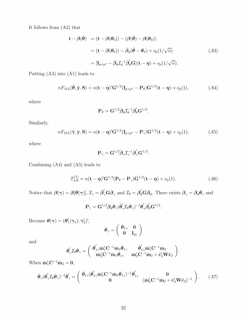
It follows from (A2) that

t − β(θ) = (t − β(θ0)) − (β(θ) − β(θ0))

= (t − β(θ0)) − βθ(θ − θ0) + op(1/√n)

= [Ip+p∗ − βθI−1θ β

′θG](t − η) + op(1/

√n).

(A3)

Putting (A3) into (A1) leads to

nFML(θ, y,S) = n(t − η)′G1/2(Ip+p∗ − Pθ)G1/2(t − η) + op(1), (A4)

where

Pθ = G1/2βθI−1θ β

′θG

1/2.

Similarly,

nFML(γ, y,S) = n(t − η)′G1/2(Ip+p∗ − Pγ)G1/2(t − η) + op(1), (A5)

where

Pγ = G1/2βγI−1γ β

′γG

1/2.

Combining (A4) and (A5) leads to

T(1)LR = n(t − η)′G1/2(Pθ − Pγ)G

1/2(t − η) + op(1). (A6)

Notice that β(γ) = β[θ(γ)], Iγ = β′γGβγ and Iθ = β

′θGβθ. There exists βγ = βθθγ and

Pγ = G1/2βθθγ(θ′γIθθγ)−1θ

′γβ

′θG

1/2.

Because θ(γ) = (θ′1(γ1),γ′2)

′,

θγ =

(θ1γ 00 Iq2

)

and

θ′γIθθγ =

(θ′1γm

′1C

−1m1θ1γ θ′1γm

′1C

−1m2

m′2C

−1m1θ1γ m′2C

−1m2 + c′2Wc2

).

When m′1C

−1m2 = 0,

θγ(θ′γIθθγ)−1θ

′γ =

(θ1γ(θ

′1γm

′1C

−1m1θ1γ)−1θ

′1γ 0

0 (m′2C

−1m2 + c′2Wc2)−1

). (A7)

32

It follows from (A7) that

Pθ − Pγ = G1/2βθ[I−1θ − θγ(θ

′γIθθγ)−1θ

′γ]β

′θG

1/2

=

(R 00 0

),

(A8)

where

R = C−1/2m1[(m′1C

−1m1)−1 − θ1γ(θ

′1γm

′1C

−1m1θ1γ)−1θ

′1γ]m

′1C

−1/2.

Combining (A6) and (A8) leads to

T(1)LR = z′Rz + op(1),

where z = C−1/2(y−µ)L→ N(0, Ip). The theorem follows by noticing that R is a projection

matrix with tr(R) = dim(θ1) − dim(γ1).

33

References

Algina, J., & Oshima,T. C. (1990). Robustness of the independent samples Hotelling’s T 2 to

variance-covariance heteroscedasticity when sample sizes are unequal and in small ratios.

Psychological Bulletin, 108, 308–313

Amemiya, Y. & Anderson, T. W. (1990). Asymptotic chi-square tests for a large class of

factor analysis models. Annals of Statistics, 18, 1453–1463.

Anderson, T. W. (1984). An introduction to multivariate statistical analysis (2nd ed.). New

York: Wiley.

Arnold, S. F. (1981). The theory of linear models and multivariate analysis. New York:

Wiley.

Bentler, P. M. (1968). Alpha-maximized factor analysis (Alphamax): Its relation to alpha

and canonical factor analysis. Psychometrika, 33, 335–345.

Bentler, P. M. (1995). EQS structural equations program manual. Encino, CA: Multivariate

Software.

Bagozzi, R. P. (1977). Structural equation models in experimental research. Journal of

Marketing Research, 14, 209–226.

Bagozzi, R. P., & Yi, Y. (1989). On the use of structural equation models in experimental

designs. Journal of Marketing Research, 26, 271–284.

Bentler, P. M., & Yuan, K.-H. (2000). On adding a mean structure to a covariance structure

model. Educational and Psychological Measurement, 60, 326–339.

Browne, M. W., & Arminger, G. (1995). Specification and estimation of mean and covari-

ance structure models. In G. Arminger, C. C. Clogg, & M. E. Sobel (Eds.), Handbook

of statistical modeling for the social and behavioral sciences (pp. 185–249). New York:

Plenum.

Browne, M. W., & Shapiro, A. (1988). Robustness of normal theory methods in the analysis

of linear latent variate models. British Journal of Mathematical and Statistical Psychology,

41, 193–208.

Buse, A. (1982). The likelihood ratio, Wald, and Lagrange multiplier tests: An expository

note. American Statistician, 36, 153–157.

Byrne, B. M., Shavelson, R. J., & Muthen, B. (1989). Testing for the equivalence of factorial

covariance and mean structures: The issue of partial measurement invariance. Psycholog-

ical Bulletin, 105, 456–466.

Chou, C.-P., & Bentler, P. M. (1990). Model modification in covariance structure modeling:

A comparison among likelihood ratio, Lagrange multiplier, and Wald tests. Multivariate

Behavioral Research, 25, 115–136.

34

Cohen, J. (1988). Statistical power analysis for the behavioral sciences (2nd ed.). Hillsdale,

NJ: Erlbaum.

Cole, D. A., Maxwell, S. E., Arvey, R., & Salas, E. (1993). Multivariate group comparisons

of variable systems: MANOVA and structural equation modeling. Psychological Bulletin,

114, 174–184.

Curran, P. J. (2000). A latent curve framework for the study of developmental trajectories in

adolescent substance use. In J. R. Rose, L. Chassin, C. C. Presson, & S. J. Sherman (Eds.),

Multivariate applications in substance use research: New methods for new questions (pp.

1-42). Mahwah, NJ: Erlbaum.

Curran, P. J., Bollen, K. A., Paxton, P., Kirby, J., & Chen, F. (2002). The noncentral

chi-square distribution in misspecified structural equation models: Finite sample results

from a Monte Carlo simulation. Multivariate Behavioral Research, 37, 1–36.

Duncan, T. E., Duncan, S. C., Strycker, L. A., Li, F., & Alpert, A. (1999). An introduction

to latent variable growth curve modeling: Concepts, issues, and applications. Mahwah,

NJ: Erlbaum.

Efron, b. & Tibshirani, R. J. (1993). An introduction to the bootstrap. New York: Chapman

& Hall.

Engle, R. (1984). Wald, likelihood ratio and Lagrange multiplier tests in econometrics.

In Griliches and Intrilligator (Eds.), Handbook of econometrics, vol II (pp. 775–826).

Amsterdam: North Holland.

Ferguson, T. (1996). A course in large sample theory. London: Chapman & Hall.

Hakstian, A. R., Roed, J. C. & Lind, J. C. (1979). Two-sample T 2 procedure and the

assumption of homogeneous covariance matrices. Psychological Bulletin, 86, 1255–1263.

Hancock, G. R. (2001). Effect size, power, and sample size determination for structured

means modeling and MIMIC approaches to between-groups hypothesis testing of means

on a single latent construct. Psychometrika, 66, 373–388.

Hancock, G. R. (2003). Fortune cookies, measurement error, and experimental design. Jour-

nal of Modern Applied Statistical Methods, 2, 293–305.

Hancock, G. R., Lawrence, F. R., & Nevitt, J. (2000). Type I error and power of latent mean

methods and MANOVA in factorially invariant and noninvariant latent variable systems.

Structural Equation Modeling, 7, 534–556.

Hancock, G. R., & Mueller, R. O. (2001). Rethinking construct reliability. In R. Cudeck,

S. du Toit, & D. Sorbom (Eds.), Structural equation modeling: Present and future (pp.

195–216). Lincolnwood, IL: Scientific Software International.

Ito, K. & Schull, W. J. (1964). On the robustness of the T 20 test in multivariate analysis of

35

variance when variance-covariance matrices are not equal. Biometrika, 51, 71-82.

Kano, Y. (1986). Conditions on consistency of estimators in covariance structure model.

Journal of the Japan Statistical Society, 16, 75–80.

Kano, Y. (1995). An asymptotic expansion of the distribution of Hotelling’s T 2-statistic un-

der general distributions. American Journal of Mathematical and Management Sciences,

15 317–341.

Kano, Y. (2001). Structural equation modeling for experimental data. In R. Cudeck, S.H.C.

du Toit, & D. Sorbom (Eds.), Structural equation modeling: Present and future (pp.

381–402). Lincolnwood, IL: Scientific Software International.

Kaplan, D., & George, R. (1995). A study of the power associated with testing factor

mean differences under violations of factorial invariance. Structural Equation Modeling,

2, 101–118.

Kuhnel, S. M. (1988). Testing MANOVA designs with LISREL. Sociological Methods and

Research, 16, 504–523.

Li, H. (1997). A unifying expression for the maximal reliability of a linear composite. Psy-

chometrika, 62, 245–249.

MacCallum, R. C., Browne, M. W., & Sugawara, H. M. (1996). Power analysis and de-

termination of sample size for covariance structure modeling. Psychological Methods, 1,

130–149.

Magnus, J. R., & Neudecker, H. (1999). Matrix differential calculus with applications in

statistics and econometrics. New York: Wiley.

McArdle, J. J., & Epstein, D. (1987). Latent growth curves with developmental structure

equation models. Child Development, 58, 110–133.

Meredith, W., & Tisak, J. (1990). Latent curve analysis. Psychometrika, 55, 107–122.

Muthen, B. (1989). Latent variable modeling in heterogeneous populations. Psychometrika,

54, 557–585.

Raykov, T. (2004). Estimation of Maximal Reliability: A Note on a Covariance Struc-

ture Modeling Approach. To appear in British Journal of Mathematical and Statistical

Psychology, 57.

Rudin, W. (1976). Principles of mathematical analysis (3rd ed.). New York: McGraw-Hill.

Satorra, A. (1989). Alternative test criteria in covariance structure analysis: A unified

approach. Psychometrika, 54, 131–151.

Satorra, A., & Bentler, P. M. (1990). Model conditions for asymptotic robustness in the

analysis of linear relations. Computational Statistics & Data Analysis, 10, 235–249.

36

Satorra, A. & Saris, W. (1985). Power of the likelihood ratio test in covariance structure

analysis. Psychometrika, 50, 83–90.

Shapiro, A. (1984). A note on the consistency of estimators in the analysis of moment

structures. British Journal of Mathematical and Statistical Psychology, 37, 84–88.

Sorbom, D. (1974). A general method for studying differences in factor means and factor

structures between groups. British Journal of Mathematical and Statistical Psychology,

27, 229–239.

Steiger, J. H., Shapiro, A., & Browne, M. W. (1985). On the multivariate asymptotic

distribution of sequential chi-square statistics. Psychometrika, 50, 253–264.

Stroud, T. W. F. (1972). Fixed alternatives and Wald’s formulation of the noncentral asymp-

totic behavior of the likelihood ratio statistic. Annals of Mathematical Statistics, 43,

447–454.

Wakaki, H., Yanagihara, H., & Fujikoshi, Y. (2002). Asymptotic expansions of the null distri-

butions of test statistics for multivariate linear hypothesis under nonnormality. Hiroshima

Mathematical Journal, 32, 17–50.

Yuan, K.-H., & Bentler, P. M. (1998). Normal theory based test statistics in structural

equation modeling. British Journal of Mathematical and Statistical Psychology, 51, 289–

309.

Yuan, K.-H., & Bentler, P. M. (1999). On normal theory and associated test statistics

in covariance structure analysis under two classes of nonnormal distributions. Statistica

Sinica, 9, 831–853.

Yuan, K.-H., & Bentler, P. M. (2002). On robustness of the normal-theory based asymptotic

distributions of three reliability coefficient estimates. Psychometrika, 67, 251–259.

Yuan, K.-H., & Bentler, P. M. (in press). On chi-square difference and z tests in mean

and covariance structure analysis when the base model is misspecified. Educational and

Psychological Measurement (www.nd.edu/∼kyuan/papers/nest-chisq-z.pdf).

Yuan, K.-H., Marshall, L. L., & Bentler, P. M. (2002). A unified approach to exploratory

factor analysis with missing data, nonnormal data, and in the presence of outliers. Psy-

chometrika, 67, 95–122.

Yuan, K.-H., Marshall, L. L., & Bentler, P. M. (2003). Assessing the effect of model misspec-

ifications on parameter estimates in structural equation models. Sociological Methodology,

33, 241–265.

Yung, Y.-F., & Bentler, P. M. (1999). On added information for ML factor analysis with

mean and covariance structures. Journal of Educational and Behavioral Statistics, 24,

1–20.

37

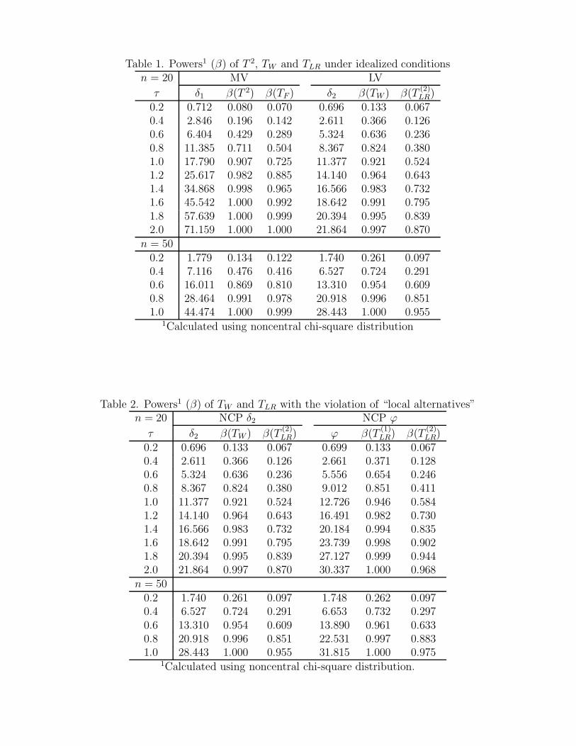
Table 1. Powers1 (β) of T 2, TW and TLR under idealized conditionsn = 20 MV LV

τ δ1 β(T 2) β(TF ) δ2 β(TW ) β(T(2)LR)

0.2 0.712 0.080 0.070 0.696 0.133 0.0670.4 2.846 0.196 0.142 2.611 0.366 0.1260.6 6.404 0.429 0.289 5.324 0.636 0.2360.8 11.385 0.711 0.504 8.367 0.824 0.3801.0 17.790 0.907 0.725 11.377 0.921 0.5241.2 25.617 0.982 0.885 14.140 0.964 0.6431.4 34.868 0.998 0.965 16.566 0.983 0.7321.6 45.542 1.000 0.992 18.642 0.991 0.7951.8 57.639 1.000 0.999 20.394 0.995 0.8392.0 71.159 1.000 1.000 21.864 0.997 0.870

n = 500.2 1.779 0.134 0.122 1.740 0.261 0.0970.4 7.116 0.476 0.416 6.527 0.724 0.2910.6 16.011 0.869 0.810 13.310 0.954 0.6090.8 28.464 0.991 0.978 20.918 0.996 0.8511.0 44.474 1.000 0.999 28.443 1.000 0.955

1Calculated using noncentral chi-square distribution

Table 2. Powers1 (β) of TW and TLR with the violation of “local alternatives”n = 20 NCP δ2 NCP ϕ

τ δ2 β(TW ) β(T(2)LR) ϕ β(T

(1)LR) β(T

(2)LR)

0.2 0.696 0.133 0.067 0.699 0.133 0.0670.4 2.611 0.366 0.126 2.661 0.371 0.1280.6 5.324 0.636 0.236 5.556 0.654 0.2460.8 8.367 0.824 0.380 9.012 0.851 0.4111.0 11.377 0.921 0.524 12.726 0.946 0.5841.2 14.140 0.964 0.643 16.491 0.982 0.7301.4 16.566 0.983 0.732 20.184 0.994 0.8351.6 18.642 0.991 0.795 23.739 0.998 0.9021.8 20.394 0.995 0.839 27.127 0.999 0.9442.0 21.864 0.997 0.870 30.337 1.000 0.968

n = 500.2 1.740 0.261 0.097 1.748 0.262 0.0970.4 6.527 0.724 0.291 6.653 0.732 0.2970.6 13.310 0.954 0.609 13.890 0.961 0.6330.8 20.918 0.996 0.851 22.531 0.997 0.8831.0 28.443 1.000 0.955 31.815 1.000 0.975

1Calculated using noncentral chi-square distribution.

Table 3. Empirical powers1 (β) of TF , T 2, TW , T(1)LR and T

(2)LR

n = 20 MV LV

τ TF β(T 2) β(TW ) β(T(1)LR) β(T

(2)LR)

0.0 0.056 0.274 0.044 0.044 0.1500.2 0.084 0.318 0.136 0.134 0.1880.4 0.154 0.436 0.376 0.376 0.2560.6 0.262 0.640 0.692 0.696 0.3540.8 0.490 0.856 0.886 0.888 0.6021.0 0.734 0.944 0.980 0.980 0.7361.2 0.894 0.990 0.996 0.996 0.8861.4 0.974 1.000 1.000 1.000 0.9521.6 0.994 1.000 1.000 1.000 0.9941.8 0.998 1.000 1.000 1.000 0.9962.0 1.000 1.000 1.000 1.000 1.000

n = 500.0 0.048 0.102 0.056 0.056 0.0620.2 0.112 0.232 0.278 0.278 0.1180.4 0.424 0.570 0.762 0.760 0.3600.6 0.822 0.904 0.986 0.986 0.7460.8 0.974 0.994 1.000 1.000 0.9301.0 1.000 1.000 1.000 1.000 0.994

1Based on 500 replications with normal data.

Table 4. Empirical NCP1

n = 20τ δ1 δ11 δ12 δ2 δ2 ϕ ϕ1 ϕ2

0.0 0.000 0.058 3.592 0.000 0.023 0.000 0.034 3.2140.2 0.712 0.926 4.966 0.696 0.717 0.699 0.747 4.0550.4 2.846 2.711 7.793 2.611 2.479 2.661 2.638 5.4610.6 6.404 5.967 12.948 5.324 5.068 5.556 5.527 8.1740.8 11.385 10.530 20.172 8.367 7.623 9.012 8.515 12.1331.0 17.790 18.087 32.138 11.377 10.747 12.726 12.650 15.8051.2 25.617 26.140 44.888 14.140 13.492 16.491 16.588 20.1171.4 34.868 34.282 57.779 16.566 15.821 20.184 20.062 23.3931.6 45.542 45.030 74.797 18.642 17.752 23.739 23.407 27.3101.8 57.639 56.714 93.297 20.394 19.319 27.127 26.806 29.9972.0 71.159 72.163 117.758 21.864 20.871 30.337 30.383 33.785

n = 500.0 0.000 -0.204 0.762 0.000 0.056 0.000 0.061 0.7410.2 1.779 1.617 2.887 1.740 1.773 1.748 1.801 2.5420.4 7.116 7.185 9.382 6.527 6.335 6.653 6.531 8.1240.6 16.011 16.084 19.765 13.310 13.292 13.890 14.050 15.1910.8 28.464 28.600 34.367 20.918 20.283 22.531 22.166 23.5081.0 44.474 44.044 52.385 28.443 27.608 31.815 31.412 32.4911.2 64.043 64.021 75.692 35.351 34.606 41.228 41.147 42.4481.4 87.170 86.642 102.082 41.416 40.584 50.460 50.275 51.1161.6 113.854 112.286 132.001 46.605 45.440 59.348 58.772 59.9631.8 144.097 140.658 165.101 50.986 49.761 67.817 67.046 68.4722.0 177.897 178.223 208.927 54.660 53.557 75.844 75.811 76.691

1Based on 500 replications with normal data.

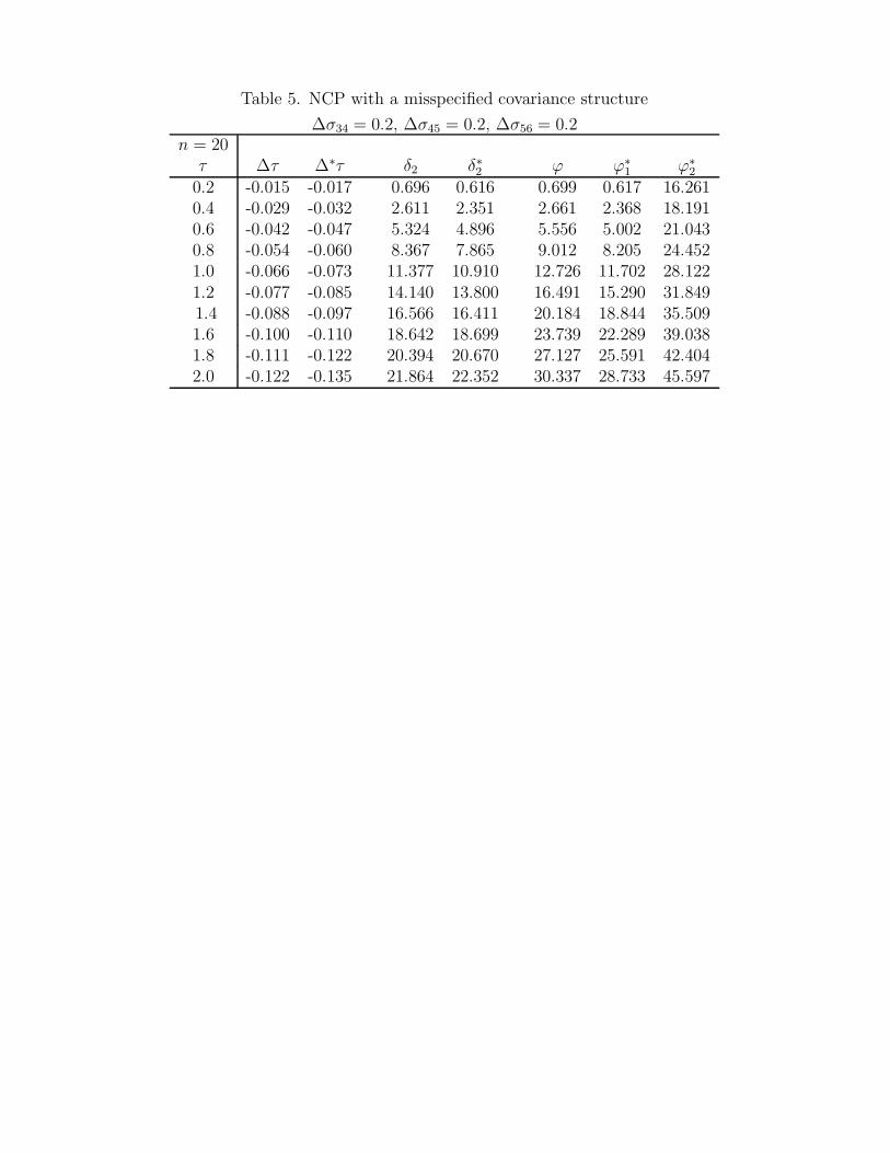
Table 5. NCP with a misspecified covariance structure

∆σ34 = 0.2, ∆σ45 = 0.2, ∆σ56 = 0.2n = 20τ ∆τ ∆∗τ δ2 δ∗2 ϕ ϕ∗

1 ϕ∗2

0.2 -0.015 -0.017 0.696 0.616 0.699 0.617 16.2610.4 -0.029 -0.032 2.611 2.351 2.661 2.368 18.1910.6 -0.042 -0.047 5.324 4.896 5.556 5.002 21.0430.8 -0.054 -0.060 8.367 7.865 9.012 8.205 24.4521.0 -0.066 -0.073 11.377 10.910 12.726 11.702 28.1221.2 -0.077 -0.085 14.140 13.800 16.491 15.290 31.8491.4 -0.088 -0.097 16.566 16.411 20.184 18.844 35.5091.6 -0.100 -0.110 18.642 18.699 23.739 22.289 39.0381.8 -0.111 -0.122 20.394 20.670 27.127 25.591 42.4042.0 -0.122 -0.135 21.864 22.352 30.337 28.733 45.597

Figure 1(a). QQ plots of the Wald statistic TF versus the noncentral F distribution

Fp,n−p(δ1), n = 20.

0 1 2 3 4 5 6 7

Central F distribution

0

2

4

6

F s

tatistic

tau=0

0 1 2 3 4 5 6 7

Noncentral F distribution

0

2

4

6

F s

tatistic

tau=0.2

3 8 13 18

Noncentral F distribution

0

5

10

15

20

F s

tatistic

tau=1.0

0 10 20 30 40 50

Noncentral F distribution

0

10

20

30

40

50

F s

tatistic

tau=1.8

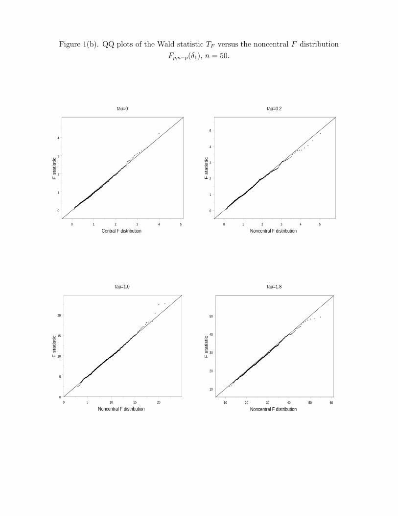
Figure 1(b). QQ plots of the Wald statistic TF versus the noncentral F distribution

Fp,n−p(δ1), n = 50.

0 1 2 3 4 5

Central F distribution

0

1

2

3

4

F s

tatistic

tau=0

0 1 2 3 4 5

Noncentral F distribution

0

1

2

3

4

5

F s

tatistic

tau=0.2

0 5 10 15 20

Noncentral F distribution

0

5

10

15

20

F s

tatistic

tau=1.0

10 20 30 40 50 60

Noncentral F distribution

10

20

30

40

50

F s

tatistic

tau=1.8

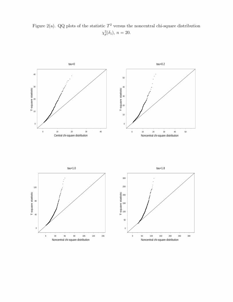
Figure 2(a). QQ plots of the statistic T 2 versus the noncentral chi-square distribution

χ2p(δ1), n = 20.

0 10 20 30 40

Central chi-square distribution

0

10

20

30

40

T-s

quare

sta

tistic

tau=0

0 10 20 30 40 50

Noncentral chi-square distribution

0

10

20

30

40

50

T-s

quare

sta

tistic

tau=0.2

5 30 55 80 105 130 155

Noncentral chi-square distribution

0

40

80

120

T-s

quare

sta

tistic

tau=1.0

0 50 100 150 200 250 300

Noncentral chi-square distribution

0

50

100

150

200

250

300

T-s

quare

sta

tistic

tau=1.8

Figure 2(b). QQ plots of the statistic T 2 versus the noncentral chi-square distribution

χ2p(δ1), n = 50.

0 5 10 15 20 25 30

Central chi-square distribution

0

10

20

30

T-s

quare

sta

tistic

tau=0

0 5 10 15 20 25 30 35

Noncentral chi-square distribution

0

10

20

30

T-s

quare

sta

tistic

tau=0.2

0 20 40 60 80 100 120 140 160

Noncentral chi-square distribution

0

50

100

150

T-s

quare

sta

tistic

tau=1.0

50 100 150 200 250 300 350

Noncentral chi-square distribution

50

100

150

200

250

300

T-s

quare

sta

tistic

tau=1.8

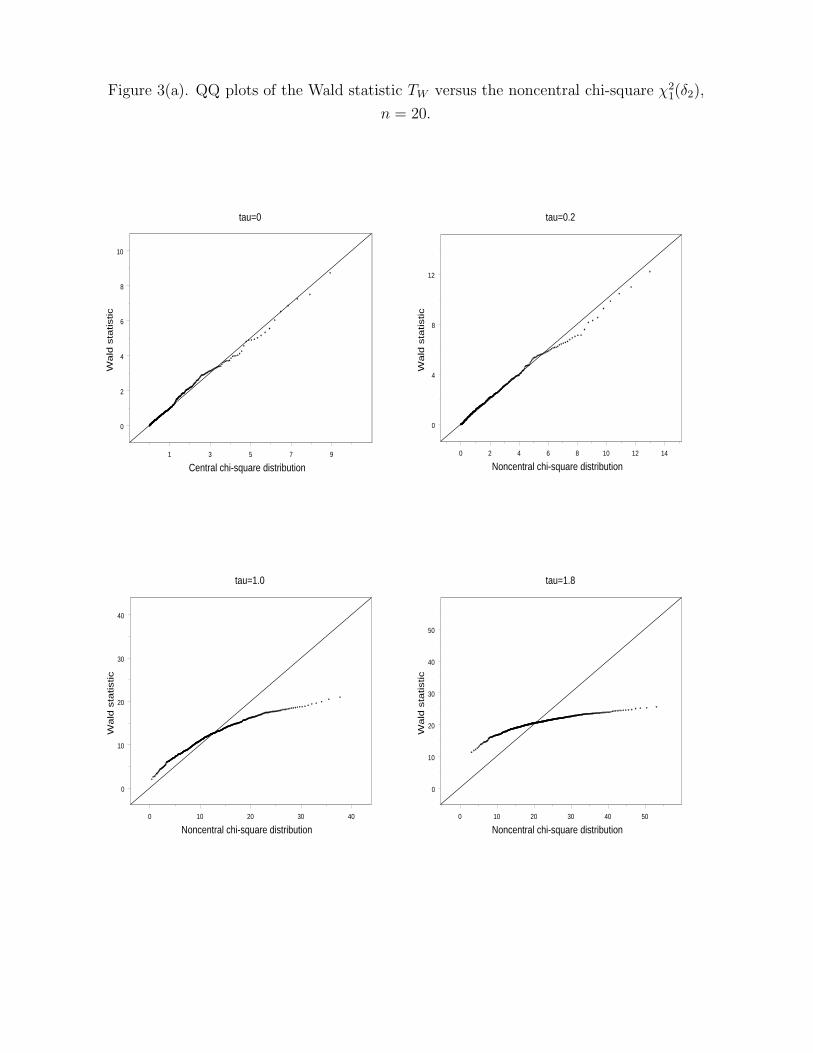
Figure 3(a). QQ plots of the Wald statistic TW versus the noncentral chi-square χ21(δ2),

n = 20.

1 3 5 7 9

Central chi-square distribution

0

2

4

6

8

10

Wald

sta

tistic

tau=0

0 2 4 6 8 10 12 14

Noncentral chi-square distribution

0

4

8

12

Wald

sta

tistic

tau=0.2

0 10 20 30 40

Noncentral chi-square distribution

0

10

20

30

40

Wald

sta

tistic

tau=1.0

0 10 20 30 40 50

Noncentral chi-square distribution

0

10

20

30

40

50

Wald

sta

tistic

tau=1.8

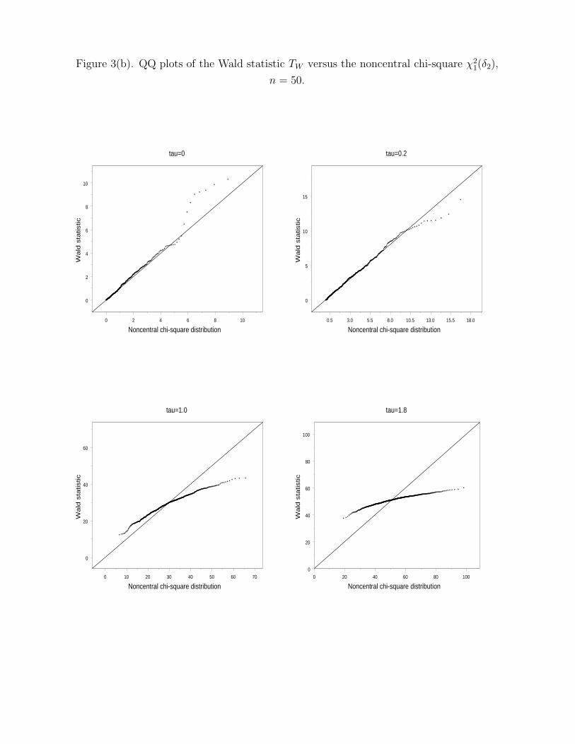
Figure 3(b). QQ plots of the Wald statistic TW versus the noncentral chi-square χ21(δ2),

n = 50.

0 2 4 6 8 10

Noncentral chi-square distribution

0

2

4

6

8

10

Wald

sta

tistic

tau=0

0.5 3.0 5.5 8.0 10.5 13.0 15.5 18.0

Noncentral chi-square distribution

0

5

10

15

Wald

sta

tistic

tau=0.2

0 10 20 30 40 50 60 70

Noncentral chi-square distribution

0

20

40

60

Wald

sta

tistic

tau=1.0

0 20 40 60 80 100

Noncentral chi-square distribution

0

20

40

60

80

100

Wald

sta

tistic

tau=1.8

Figure 4(a). QQ plots of the likelihood ratio statistic T(1)ML versus the noncentral chi-square

χ21(ϕ), n = 20.

-2 0 2 4 6 8 10 12

Central chi-square distribution

-1

3

7

11

Lik

elih

ood r

atio s

tatistic

tau=0

0 5 10 15

Noncentral chi-square distribution

-1

4

9

14

Lik

elih

ood r

atio s

tatistic

tau=0.2

0 10 20 30 40

Noncentral chi-square distribution

0

10

20

30

40

Lik

elih

ood r

atio s

tatistic

tau=1.0

0 10 20 30 40 50 60 70

Noncentral chi-square distribution

0

20

40

60

Lik

elih

ood r

atio s

tatistic

tau=1.8

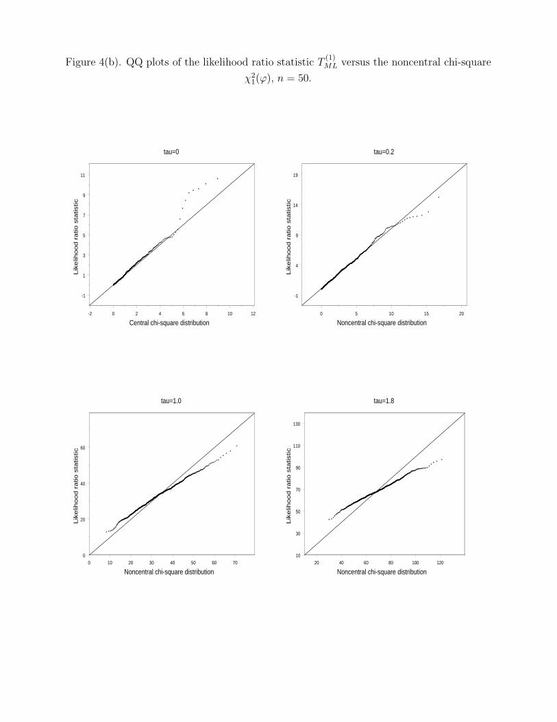
Figure 4(b). QQ plots of the likelihood ratio statistic T(1)ML versus the noncentral chi-square

χ21(ϕ), n = 50.

-2 0 2 4 6 8 10 12

Central chi-square distribution

-1

1

3

5

7

9

11

Lik

elih

ood r

atio s

tatistic

tau=0

0 5 10 15 20

Noncentral chi-square distribution

-1

4

9

14

19

Lik

elih

ood r

atio s

tatistic

tau=0.2

0 10 20 30 40 50 60 70

Noncentral chi-square distribution

0

20

40

60

Lik

elih

ood r

atio s

tatistic

tau=1.0

20 40 60 80 100 120

Noncentral chi-square distribution

10

30

50

70

90

110

130

Lik

elih

ood r

atio s

tatistic

tau=1.8

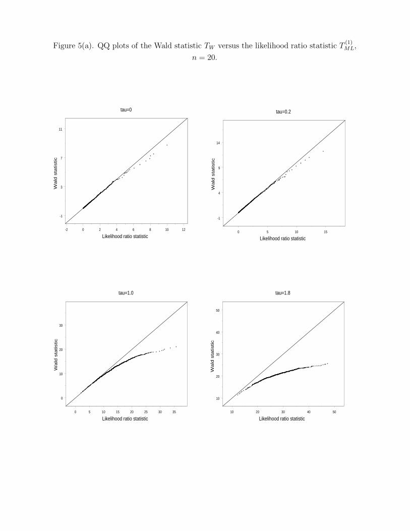
Figure 5(a). QQ plots of the Wald statistic TW versus the likelihood ratio statistic T(1)ML,

n = 20.

-2 0 2 4 6 8 10 12

Likelihood ratio statistic

-1

3

7

11

Wald

sta

tistic

tau=0

0 5 10 15

Likelihood ratio statistic

-1

4

9

14

Wald

sta

tistic

tau=0.2

0 5 10 15 20 25 30 35

Likelihood ratio statistic

0

10

20

30

Wald

sta

tistic

tau=1.0

10 20 30 40 50

Likelihood ratio statistic

10

20

30

40

50

Wald

sta

tistic

tau=1.8

Figure 5(b). QQ plots of the Wald statistic TW versus the likelihood ratio statistic T(1)ML,

n = 50.

-2 0 2 4 6 8 10 12

Likelihood ratio statistic

-1

1

3

5

7

9

11

Wald

sta

tistic

tau=0

0 5 10 15

Likelihood ratio statistic

-1

4

9

14

Wald

sta

tistic

tau=0.2

10 20 30 40 50 60

Likelihood ratio statistic

10

20

30

40

50

60

Wald

sta

tistic

tau=1.0

30 50 70 90

Likelihood ratio statistic

20

40

60

80

100

Wald

sta

tistic

tau=1.8

Figure 6(a). QQ plots of the likelihood ratio statistic T(2)ML versus the noncentral chi-square

χ215(ϕ), n = 20.

0 10 20 30 40 50 60

Central chi-square distribution

0

20

40

60

Lik

elih

ood r

atio s

tatistic

tau=0

0 10 20 30 40 50 60

Noncentral chi-square distribution

0

10

20

30

40

50

60

Lik

elih

ood r

atio s

tatistic

tau=0.2

0 10 20 30 40 50 60

Noncentral chi-square distribution

0

20

40

60

Lik

elih

ood r

atio s

tatistic

tau=1.0

0 10 20 30 40 50 60 70 80

Noncentral chi-square distribution

0

20

40

60

80

Lik

elih

ood r

atio s

tatistic

tau=1.8

Figure 6(b). QQ plots of the likelihood ratio statistic T(2)ML versus the noncentral chi-square

χ215(ϕ), n = 50.

0 10 20 30 40 50

Central chi-square distribution

0

10

20

30

40

50

Lik

elih

ood r

atio s

tatistic

tau=0

0 10 20 30 40 50

Noncentral chi-square distribution

0

10

20

30

40

50

Lik

elih

ood r

atio s

tatistic

tau=0.2

0 20 40 60 80

Noncentral chi-square distribution

0

20

40

60

80

Lik

elih

ood r

atio s

tatistic

tau=1.0

40 60 80 100 120 140

Noncentral chi-square distribution

40

60

80

100

120

140

Lik

elih

ood r

atio s

tatistic

tau=1.8