mean field growth modeling with cobb-douglas … applications of mfgs in economic growth references...

BackgroundApplications of MFGs in economic growth

References

Mean Field Growth Modeling with Cobb-DouglasProduction and Relative Consumption

Minyi Huang

School of Mathematics and StatisticsCarleton UniversityOttawa, Canada

Mean Field Games and Related Topics–IIIHenri Poincare Institute, June 2015

Joint work with Son Luu Nguyen, Univ. Puerto Rico

Minyi Huang Mean Field Growth Modeling with Cobb-Douglas Production and Relative Consumption


References

Outline of talk

I Brief overview of the mean field game (MFG) equation system

I We present an application to continuous time growth problems

I Cobb-Douglas productionI HARA utilityI Absolute and relative consumptionI Product form coupling

=⇒ simple solution

I References



References

The game as an interacting particle system: review

A game of N agents (players), 1 ≤ i ≤ N. Dynamics and costs:

dxi =1

N

N∑j=1

f (xi , ui , xj)dt +1

N

N∑j=1

σ(xi , ui , xj)dwi , each xj ∈ Rn

Ji (ui , u−i ) = E

∫ T

0

1

N

N∑j=1

L(xi , ui , xj)dt, 1 ≤ i ≤ N.

(u−i : controls of all players other than player i)

Write δ(N)x = 1

N

∑Nj=1 δxj where δ• is the dirac measure.

For φ = f , σ, L, denote

1

N

N∑j=1

φ(xi , ui , xj) =

∫Rn

φ(xi , ui , y)δ(N)x (dy) := φ[xi , ui , δ

(N)x ]



References

The twin equations: HJB–McKV

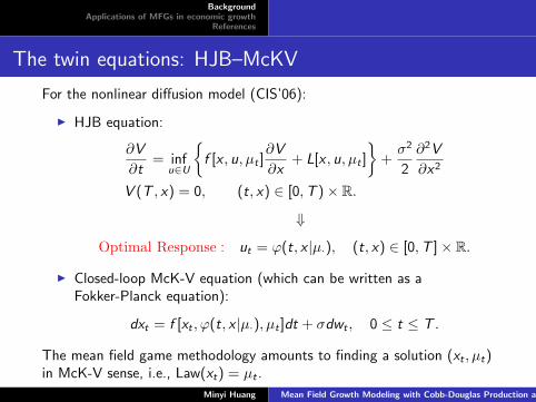
For the nonlinear diffusion model (CIS’06):

I HJB equation:

∂V

∂t= inf

u∈U

{f [x , u, µt ]

∂V

∂x+ L[x , u, µt ]

}+

σ2

2

∂2V

∂x2

V (T , x) = 0, (t, x) ∈ [0,T )× R.

⇓

Optimal Response : ut = φ(t, x |µ·), (t, x) ∈ [0,T ]× R.

I Closed-loop McK-V equation (which can be written as aFokker-Planck equation):

dxt = f [xt , φ(t, x |µ·), µt ]dt + σdwt , 0 ≤ t ≤ T .

The mean field game methodology amounts to finding a solution (xt , µt)in McK-V sense, i.e., Law(xt) = µt .



References

Recent applications

Mean field control theory has very wide current and potentialapplications (see HN’15 (submitted to CDC’15) for references):

I Economic theory

I Finance

I Communication networks

I Social opinion formation

I Power systems

I Electric vehicle recharging control

I Public health (vaccination games)

I ......



References

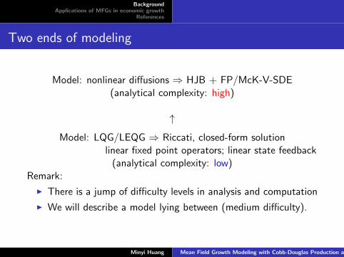
Two ends of modeling

Model: nonlinear diffusions ⇒ HJB + FP/McK-V-SDE(analytical complexity: high)

↑

Model: LQG/LEQG ⇒ Riccati, closed-form solutionlinear fixed point operators; linear state feedback(analytical complexity: low)

Remark:

I There is a jump of difficulty levels in analysis and computation

I We will describe a model lying between (medium difficulty).



References

Our goals

I Addressing mean field interactions in endogenous stochasticgrowth models with many firms

I Good mathematical tractability



References

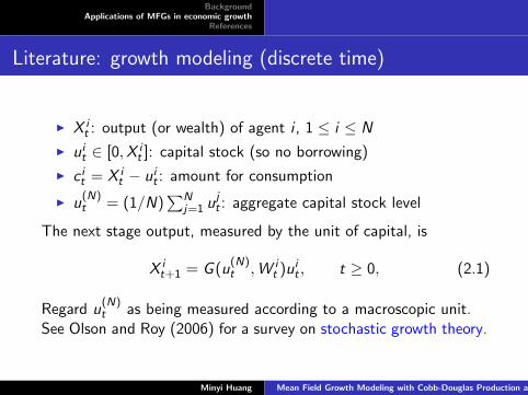
Literature: growth modeling (discrete time)

I X it : output (or wealth) of agent i , 1 ≤ i ≤ N

I uit ∈ [0,X it ]: capital stock (so no borrowing)

I c it = X it − uit : amount for consumption

I u(N)t = (1/N)

∑Nj=1 u

jt : aggregate capital stock level

The next stage output, measured by the unit of capital, is

X it+1 = G (u

(N)t ,W i

t )uit , t ≥ 0, (2.1)

Regard u(N)t as being measured according to a macroscopic unit.

See Olson and Roy (2006) for a survey on stochastic growth theory.



References

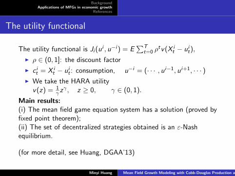
The utility functional

The utility functional is Ji (ui , u−i ) = E

∑Tt=0 ρ

tv(X it − uit),

I ρ ∈ (0, 1]: the discount factor

I c it = X it − uit : consumption, u−i = (· · · , ui−1, ui+1, · · · )

I We take the HARA utilityv(z) = 1

γ zγ , z ≥ 0, γ ∈ (0, 1).

Main results:(i) The mean field game equation system has a solution (proved byfixed point theorem);(ii) The set of decentralized strategies obtained is an ε-Nashequilibrium.

(for more detail, see Huang, DGAA’13)



References

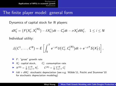
The finite player model: general form

Dynamics of capital stock for N players:

dX it = {F (X i

t ,X(N)t )− δX i

t }dt − C itdt − σX i

t dWit , 1 ≤ i ≤ N

Individual utility:

Ji (C1, . . . ,CN) = E

[∫ T

0e−ρtU(C i

t ,C(N)t )dt + e−ρTS(X i

T )

],

I F : “gross” growth rate

I X it : capital stock, C i

t : consumption rate

I X (N) = 1N

∑Nj=1 X

jt , C (N) = 1

N

∑Nj=1 C

jt

I δdt + dW it : stochastic depreciation (see e.g. Walde’11, Feicht and Stummer’10

for stochastic depreciation modeling)



References

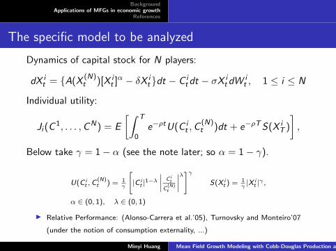
The specific model to be analyzed

Dynamics of capital stock for N players:

dX it = {A(X (N)

t )[X it ]α − δX i

t }dt − C itdt − σX i

t dWit , 1 ≤ i ≤ N

Individual utility:

Ji (C1, . . . ,CN) = E

[∫ T

0e−ρtU(C i

t ,C(N)t )dt + e−ρTS(X i

T )

],

Below take γ = 1− α (see the note later; so α = 1− γ).

U(C it ,C

(N)t ) = 1

γ

[|C i

t |1−λ

∣∣∣∣ C it

C(N)t

∣∣∣∣λ]γ

S(X it ) =

1γ|X i

t |γ ,

α ∈ (0, 1), λ ∈ (0, 1)

I Relative Performance: (Alonso-Carrera et al.’05), Turnovsky and Monteiro’07

(under the notion of consumption externality, ...)



References

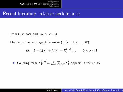
Recent literature: relative performance

From (Espinosa and Touzi, 2013)

The performance of agent (manager) i (i = 1, 2, . . . ,N):

EU[(1− λ)X i

T + λ(X iT − X

(−i)T )

], 0 < λ < 1

I Coupling term X(−i)T = 1

N−1

∑j =i X

jT appears in the utility



References

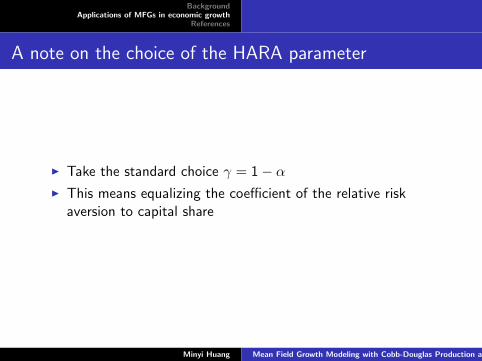
A note on the choice of the HARA parameter

I Take the standard choice γ = 1− α

I This means equalizing the coefficient of the relative riskaversion to capital share



References

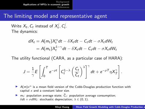
The limiting model and representative agent

Write Xt ,Ct instead of X it ,C

it .

The dynamics:

dXt = A(mt)Xαt dt − δXtdt − Ctdt − σXtdWt

= A(mt)X1−γt dt − δXtdt − Ctdt − σXtdWt

The utility functional (CARA, as a particular case of HARA):

J =1

γE

[∫ T

0e−ρt

[C 1−λt

(Ct

Ct

)λ]γ

dt + e−ρTηX γT

].

I A(m)xα is a mean field version of the Cobb-Douglas production function withcapital x and a constant labor size.

I mt : population average state; Ct : population average consumption;δdt + σdWt : stochastic depreciation; λ ∈ (0, 1).



References

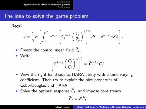
The idea to solve the game problem

Recall

J =1

γE

[∫ T

0e−ρt

[C 1−λt

(Ct

Ct

)λ]γ

dt + e−ρTηX γT

].

I Freeze the control mean field Ct .I Write [

C 1−λt

(Ct

Ct

)λ]γ

= C−λγt C γ

t

I View the right hand side as HARA utility with a time-varyingcoefficient. Then try to exploit the nice properties ofCobb-Douglas and HARA

I Solve the optimal response Ct , and impose consistency

Ct = ECt



References

The HJB

Write bt = Cλγγ−1t . The HJB reads

ρV (t, x) = Vt +σ2x2

2Vxx + (A(mt)x

1−γ − δx)Vx +1− γ

γbtV

γγ−1x .

V (T , x) =ηxγ

γ, x > 0

We look for a solution of the form

V (t, x) =1

γ[p(t)xγ + h(t)], x > 0, t ≥ 0

By consistent mean field approximations, we will derive a fixedpoint equation for bt .



References

HJB/McKV-SDE gives ...

Denote Xt = Z1γt . The HJB/McKV-SDE reduces to

p(t) =[ρ+ σ2γ(1−γ)

2 + δγ]p(t)− (1− γ)btp

γγ−1 (t), p(T ) = η

h(t) = ρh(t)− A(mt)γp(t), h(T ) = 0

dZt ={γA(mt)− γ

[δ − bt(p(t))

1γ−1 − σ2(1−γ)

2

]Zt

}dt − γσZtdWt ,

The consistency condition (replicating Ct means replicating btaccordingly)

mt = EZ1γt (= EXt), bt = [btp

1γ−1 (t)EXt ]

λγ1−γ (RHS is (ECt)

λγ1−γ )

I Existence = fixed point problem (Huang and Nguyen’15) .

I Equilibrium strategy Ct = btp1

γ−1 (t)Xt



References

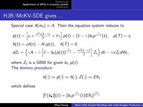
HJB/McKV-SDE gives ...

Special case A(mt) ≡ A. Then the equation system reduces to

p(t) =[ρ+ σ2γ(1−γ)

2 + δγ]p(t)− (1− γ)btp

γγ−1 (t), p(T ) = η

h(t) = ρh(t)− Aγp(t), h(T ) = 0

dZt ={γA− γ

[δ − bt(p(t))

1γ−1 − σ2(1−γ)

2

]Zt

}dt − γσZtdWt ,

where Zt is a GBM for given bt , p(t).The domino procedure:

b(·) ⇒ p(·) ⇒ h(·),Z (·) ⇒ EXt

which defines

[Γ(b•)](t) = [btp1

γ−1 (t)EXt ]λγ1−γ



References

Fixed point

The solution of HJB/McKV-SDE reduces to analyzing the fixedequation

bt = [Γ(b•)](t)

Existence result: There exists a solution bt (which furtherdetermines p(t), h(t),Zt) for small λ.

Proof. Schauder’s fixed point theorem.



References

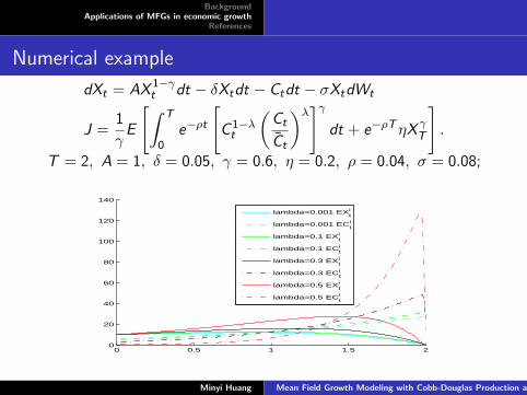
Numerical example

dXt = AX 1−γt dt − δXtdt − Ctdt − σXtdWt

J =1

γE

[∫ T

0e−ρt

[C 1−λt

(Ct

Ct

)λ]γ

dt + e−ρTηX γT

].

T = 2, A = 1, δ = 0.05, γ = 0.6, η = 0.2, ρ = 0.04, σ = 0.08;

0 0.5 1 1.5 20

20

40

60

80

100

120

140

lambda=0.001 EXti

lambda=0.001 ECti

lambda=0.1 EXti

lambda=0.1 ECti

lambda=0.3 EXti

lambda=0.3 ECti

lambda=0.5 EXti

lambda=0.5 ECti



References

Observations from numerical solutions

I The existence proof via fixed point theorem needs small λ (sothat the nonlinear mapping does not escape from a prior set).

I In practice, numerical convergence is seen for large λ.

What difference the relative performance makes?

I The numerical solution suggests agents tend to be thriftierduring the early phase if they care more about relativeconsumption (larger λ).



References

Back to the N player model?

I The proof of an ε-Nash equilibrium theorem is of interest.

I Need very careful estimate of a denominator term (checkdecay, large deviations, etc)

Recall the approximation

1

γ

|C it |1−λ

∣∣∣∣∣ C it

C(N)t

∣∣∣∣∣λγ

→ 1

γ

[|C i

t |1−λ

∣∣∣∣C it

Ct

∣∣∣∣λ]γ



References

Some applications of MFGs to economic growth and finance.

I Gueant, Lasry and Lions (2011): human capital optimization

I Lucas and Moll (2011): Knowledge growth and allocation of time

I Carmona and Lacker (2013): Investment of n brokers

I Huang (2013): capital accumulation with congestion effect

I Lachapelle et al. (2013): price formation

I Espinosa and Touzi (2013): Optimal investment with relativeperformance concern (depending on 1

N−1

∑j = Xj )

I Jaimungal and Nourian (2014): Optimal execution

I more ......



References

Thank you!


mean field growth modeling with cobb-douglas … applications of mfgs in economic growth references...

Documents