mean flow characteristics, vertical structures and bed shear stress at open channel...

Journal of Applied Research in Water and Wastewater 7(2017) 299-304

Please cite this article as: A. Safarzadeh, B. Khaiatrostami, Mean flow characteristics, vertical structures and bed shear stress at open channel bifurcation,

Journal of Applied Research in Water and Wastewater, 4(1), 2017, 299-304.

Original paper

Mean flow characteristics, vertical structures and bed shear stress at open channel bifurcation

Akbar Safarzadeh1,*, Babak Khaiatrostami2

1Department of Engineering, University of Mohaghegh Ardabili, Iran. 2Research Department, Ardabil Regional Water Co., Iran.

ARTICLE INFO

ABSTRACT

Article history: Received 5 February 2017 Received in revised form 29 March 2017 Accepted 14 April 2017

Water supply from rivers is accomplished with flow diversion through an intake structure. A lateral intake like bifurcation is the simplest method to withdraw water. However, flow at a channel bifurcation is turbulent, highly three-dimensional (3D) and so has many complex features. This paper reports a 3D numerical investigation of these features in an open channel flow. Simulations have been done on rectangular channel geometry, with smooth bed and sidewalls. The standard k-ɛ, k-ω model of the Wilcox, and RSM turbulence models are compared using the commercial code FLUENT. The simulation results have been compared with available experimental data. It was found that all of the turbulence models tested here accurately predicted velocity profiles in the main channel but in the branch channel, the RSM model with the k-ω model performing better than the k-ɛ model. Predicted flow physics are in close agreement with previously reported experimental results.

©2017 Razi University-All rights reserved.

Keywords: Dividing flow CFD Secondary flow Turbulence model Sediment transport

1. Introduction

Rivers are a major source of water for meeting various demands.

Usually, water supply from rivers is accomplished with flow diversion through an intake structure. River flow often transports sediment and designers are faced with the problem of sediment entering the canals and water conveyance systems. The art of the designer is to keep the amount of sediment entering the diversion system to a minimum.

A lateral intake is the simplest method of flow withdrawal. In spite of its simple layout, using this system leads to complex flow patterns and sedimentation problems at the junction region. Flow through lateral intakes is turbulent and highly three-dimensional consisting of secondary vortices and flow separation (Neary et al. 1996; Neary and Odgaard 1993).

The complex flow patterns can lead to sediment deposition in the intake channel (Barkdoll 1997 and Abbasi 2003). The past numerical studies of diversion flows have been mostly two-dimensional. Liepsch et al. (1982); Hayes et al. (1989); and Lee and Chiu (1992) have reported laminar flow calculations. 3D numerical investigations of laminar flow through lateral intakes have been reported by Neary and Sotiropoulos (1996). They employed a finite-volume method and used a non-staggered computational grid and demonstrated the relationship between singular points in the wall shear stress field and patterns of bed-load movement observed in the laboratory. Two-dimensional turbulent flow simulations have been reported by Shettar and Murthy (1996). They used depth-averaged mean flow equations closed with the k-ɛ model with standard wall functions. They are the only researchers that considered the effect of water surface variations on the flow characteristics in the junction region. Issa and Oliveira (1994) are the first researchers that have reported a 3D turbulent flow simulation for T-junction flow. They employed the Reynolds-averaged Navier-Stokes equations in conjunction with the k-ɛ turbulence model. Neary et al. (1999) conducted a 3D turbulent flow simulation for this problem. They employed 3D Reynolds-averaged equations closed with the k-ω model. They used the experimental measurements of Barkdoll (1997) for validation. None of the reviewed studies have

attempted to compare the results of different turbulence models to identify the proper model for this problem. In this paper FLUENT, a commercially-available CFD software, has been used for simulating the turbulent flow structure through a lateral intake. The standard k-ɛ, k-ω model of Wilcox, and the Reynolds stress model (RSM) turbulence closure schemes are used to simulate the turbulent flow through lateral intakes in open channels and the results are compared to published experimental data.

1.1. Objectives

In this study, a 3D numerical investigation is carried out for

turbulent incompressible flows through a 90-degree rectangular diversion. The objective of this work is twofold: (i) to identify the proper turbulence model for this problem; and (ii) to analyze the numerical solution in order to know the complex physics of diversion flows with emphasis on velocity profile variation along the main channel and branch channel, flow topology patterns, and shear stress variations on the solid boundaries.

2. Test case

As mentioned before, the experimental measurements of

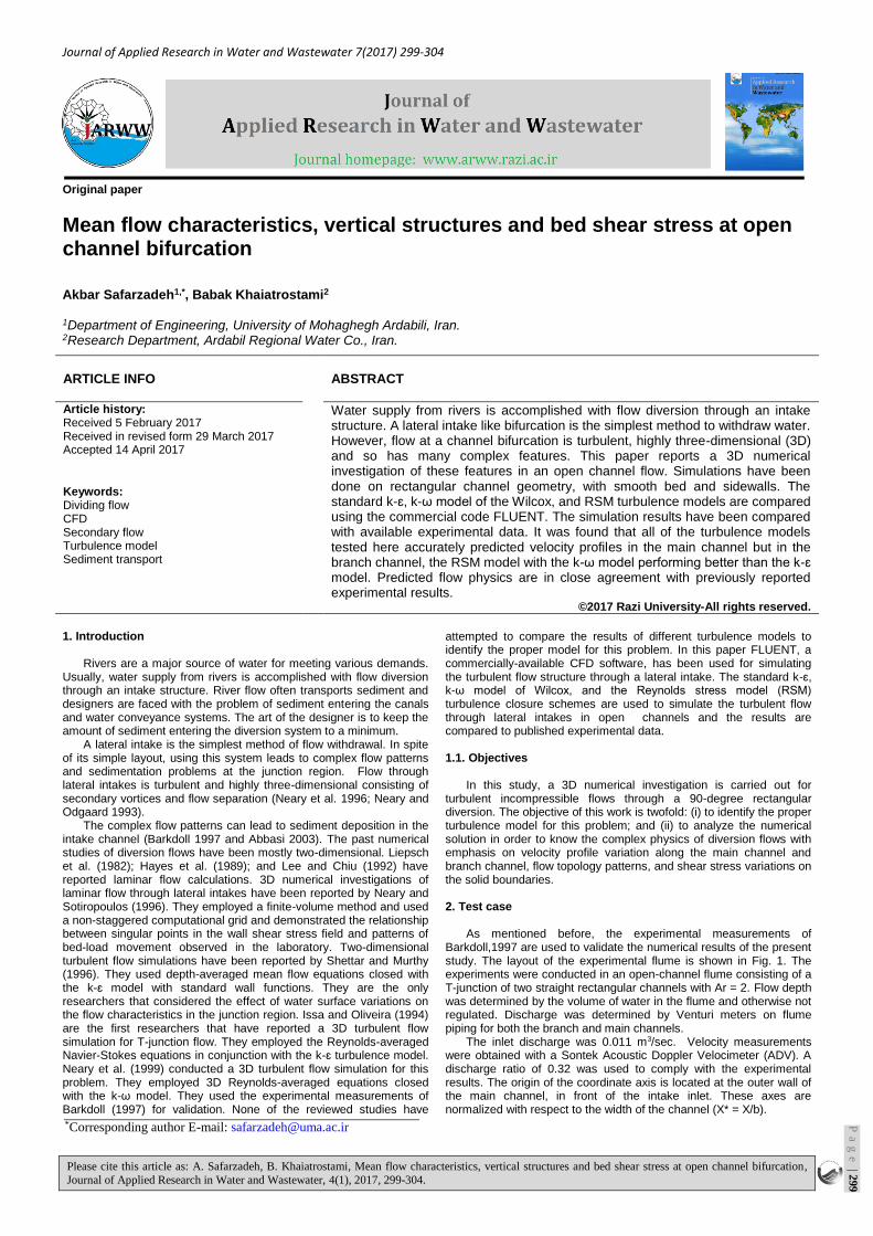
Barkdoll,1997 are used to validate the numerical results of the present study. The layout of the experimental flume is shown in Fig. 1. The experiments were conducted in an open-channel flume consisting of a T-junction of two straight rectangular channels with Ar = 2. Flow depth was determined by the volume of water in the flume and otherwise not regulated. Discharge was determined by Venturi meters on flume piping for both the branch and main channels.

The inlet discharge was 0.011 m3/sec. Velocity measurements were obtained with a Sontek Acoustic Doppler Velocimeter (ADV). A discharge ratio of 0.32 was used to comply with the experimental results. The origin of the coordinate axis is located at the outer wall of the main channel, in front of the intake inlet. These axes are normalized with respect to the width of the channel (X* = X/b).

*Corresponding author E-mail: [email protected]

Pa

ge

| 299

Safarzadeh and Khaiatrostami / J. App. Res. Wat. Wast. 7(2017) 299-304



Fig. 1. Geometrical properties of the test case

3. Governing equations 3.1. Mean flow equations

For an incompressible fluid flow, the equation of continuity and

balance of momentum for the mean motion, in Cartesian coordinates are given as (FLUENT, Inc., 1993):

0i

i

U

x

(1)

2iji i

j

RU UPU g xx x x x xij i j j j

(2)

where Ui is the mean velocity, Xi is the position, P is the mean pressure, g is the gravity accelartion and μ is the dynamic viscosity. In

Eq. 2, ' '

ij i jR u u denotes the Reynolds stress tensor. Here u′i =

ui–Ui, is the ith fluid fluctuation velocity component. This parameter is modeled using the Boussinesq’s assumption:

' ' 22

3i j t ij iju u S k (3)

where, μt is the eddy viscosity. Sij and k are mean rate of strain tensor and turbulent kinetic energy respectively and are defined as follows:

1( )

2

jiij

j i

UUS

x x

(4)

' '1( )

2i ik u u (5)

3.2. Turbulence closure equations

The standard k-ɛ and the k-ω model of Wilcox and Reynolds

stress model (RSM) turbulence closure schemes are used for turbulence modeling. In this research, these models are employed and the proper model is selected for further investigation of flow structure at this field.

3.2.1. Standard k-ε turbulence model

According to this model, the eddy viscosity is related to the

turbulence kinetic energy (k) and its rate of dissipation (ɛ) (Celik, 1999):

2

tk

c

(6)

The turbulence quantities k and ε are calculated by the following

transport equations:

xj

U

x

U

x

Uv

x

kv

xx

kU i

i

j

j

i

t

ik

t

ii

i (7)

kcP

kc

x

v

xxU

i

t

ii

i

2

21

(8)

G is the turbulence production by mean shear modeled as follows:

( )ji i

tj i j

UU UG

x x x

(9)

Closure coefficients used at this model are summarized in Table 1

(Celik, 1999).

Table 1. Closure coefficients used in k-ɛ model.

Cµ Cɛ1 Cɛ2 δk δɛ

0.09 1.44 1.92 1.00 1.30

3.2.2. k-ω turbulence model

This model has been given by Wilcox (1988, 1994). In contrast to

the k-ɛ model, which solves for the dissipation (ɛ) or rate of destruction of turbulent kinetic energy, the k-ω model solves for only the rate at which the dissipation occurs (the turbulent frequency, ω). Dimensionally ω can be related to ɛ by ω = ɛ / k (Celik, 1999):

kt (10)

The turbulence quantities k and ω are calculated by the following

transport equations:

* *1( )i t

i i i

k kU G k

x x R x

(11)

21

G

kxv

RxxU

i

t

ii

i (12)

Closure coefficients used at this model are summarized in Table 2

(Celik, 1999).

Table 2. Closure coefficients used in k-ω model.

α Β* Β σ* σ

5/9 9/100 3/40 ½ ½

3.2.3. RSM turbulence model

The Reynolds stress model (RSM) solves the Reynolds-averaged

Navier-Stokes equations by using the Reynolds stresses transport equations (seven-equations for 3D flow) and an equation for the dissipation rate, ɛ. The RSM accounts for the effects of the streamline curvature, vorticity, circulation, and rapid changes in the strain rate in a more efficient way than the two-equation models; however, it requires more computational effort and time. The transport equation in this model is as Eq. 9 (Launder, 1989, a and b).

Left hand side terms of Eq. 9 are the local time derivatives and convection term (Cij) respectively. Terms of the right hand side are turbulent diffusion (DT,ij), molecular diffusion (DL,ij), stress production (Pij), pressure strain (Φij), dissipation (ɛij) and production by system rotation (Fij), respectively. Most of the terms in this transport equation, including Cij , DL,ij , Pij do not require any modeling and are directly P

ag

e | 3

00




solved. However, DT,ij (Lien and Leschziner, 1994), Φij and ɛij (Gibson and Launder, 1978; Launder, 1989a and b) need to be modeled to close the transport equation. To simulation the pressure strain the linear pressure-strain method is used.

( ) ( )

( ) ( )

( )

( )

2 ( )

2 ( )

i j k i jk

i j k kj i ik jk

i jk k

j ji ii k j k

k k j i

ji

k k

k j m ikm i m jkm

u u u u ut x

u u u p u ux

u ux x

u uu uu u u u p

x x x x

uu

x x

u u u u

(13)

4. Numerical solution

The CFD code used in this work is version 6.0.12 of Fluent. This

software allows the solution of the three-dimensional Navier-Stokes equations in order to calculate the flow field. This code uses a finite-volume discretization method in conjunction with different turbulence models. Different schemes such as Second Order Upwind, SOU, Power Law and Quick may be used to discretize the convection terms of the transport equations. Pressure and velocity field coupling may be done by SIMPLE, SIMPLEC and PISO algorithms. Flow geometries are constructed using Gambit Software. Flow field boundary conditions and mesh generations were done by this software [8]. For this study, due to existence of circulation and separation zones in the flow field, the convection term has been discretized using the SOU scheme. Staggered meshes in conjunction with SIMPLE algorithm have been used for flow field solution. The convergence criterion is set to 10e-5.

4.1. Boundary condition

At the main channel inlet, the “Velocity Inlet” boundary condition

has been used. The flow properties at the channel inlet are shown at Table 3 (Barkdoll, 1996). The flow is subcritical and has a turbulent regime. The velocity field and turbulence parameters (k,ɛ and ω) are imposed from a separate simulation of fully developed turbulent flow through a straight channel.

At the exits of both the main and branch channels, the “outflow” boundary condition has been used. This condition states that the gradients of all variables (except pressure) are zero in the flow direction. At these boundaries, the flow often reaches a fully developed state. To ensure that this condition was satisfied at the exit of the diversion (a fully developed separation eddy); this channel was lengthened to 2.2 meters. The experimental length of the main channel was recognized to be adequate.

Table 3. Flow properties at inlet section.

Discharge(Q1) (lit/sec)

Froude Number

Reynolds Number

11 0.13 49600

The inlet discharge has been apportioned between channels. The

Discharge ratio (r = Q2/Q1= 0.32) was imposed to the exit of the diversion. Taylor showed that for discharge ratios between 0 and 0.45 and Froude numbers in the main channel between 0 and 0.4, there is less than 2% variation in flow depth in the vicinity of the diversion (Taylor, 1944). Using these points, the “Symmetry” boundary condition has been used to model the free surface. At the solid boundaries the “Wall” boundary condition was used. The walls were hydraulically smooth and the no-slip and no-flux conditions dictated to them. The implementation of wall boundary conditions in turbulent flows starts with the evaluation of:

wpy

y

(14)

where, Δyp is the distance of the near-wall node to the solid surface and τw is the wall shear stress. The distance of the first grid surface off the walls is important and depends on the flow conditions, wall roughness and the turbulence model that is used. The k-ɛ model uses the wall function to "bridge" the solution variables at the near-wall cells and the corresponding quantities on the wall but the k-ω model resolves the near wall region (laminar sub layer region).

4.2. Materials and methods

A three dimensional view of a typical computational mesh for a

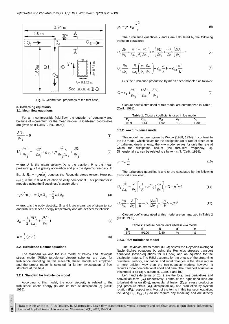
rectangular diversion configuration is shown in Fig. 2. The grid lines were clustered near the solid walls and in the junction region. To ensure the validity of the numerical solution for each turbulence model, different mesh sizes were applied to each of the models, according to the recommended selection of the near-wall cells (FLUENT 1993). Fig. 3 illustrates comparisons between measured and predicted velocity profiles using the RSM turbulence model with different mesh sizes.

A variety of mesh sizes were employed. The coarsest of the mesh sizes with similar results are shown. For the coarser of these two grid cases there were 198,620 total nodes and 220,425 for the finer grid case. The difference between the coarse and the fine grid predictions at the main channel are small enough to conclude that the coarser of the meshes be selected for the remainder of the analysis. For the k-ɛ and RSM models the total nodes were thus 198,620 while for k-ω they were 252,412. Additionally, it was found that using 10 nodes in the boundary layer for the k-ɛ and RSM turbulence models and 2 nodes in the laminar sub-layer for the k-ω model is adequate. These were determined by the guidelines in the FLUENT User’s Manual (FLUENT Inc., 1993).

Fig. 2. Computational mesh at dividing zone.

5. Results and discussion 5.1. Appropriate turbulence model

Comparisons between measured and predicted streamwise

velocity profiles near the free surface plane in both the main and branch channels for the two turbulence models employed are presented in Fig. 4. This Figure shows that all of the turbulence models used accurately predict velocity profiles in the main channel but in the branch channel, the RSM model performs very well and the k-ω model performed better than the k-ɛ turbulence model.

Comparison between measured and predicted results in Fig. 6 show that the k-ɛ model under-predicts the length of the separated flow in the intake channel but the k-ω and RSM model predictions show good agreement with the experimental results. The prediction by the k-ω model differs slightly from the experimental results, but the RSM model predicts the velocity profiles very well.

X Z

Y

Pa

ge

| 301




Fig. 3. Grid sensitivity results (only the coarsest two acceptable grid

size results shown)."Fine grid" had 220,425 computational nodes and

"Coarse grid" had 198,620. Re=49600.

Fig. 4. Comparison of turbulence model results (Near surface 2D velocity profiles).

Forward velocity maximum shifts toward the inner bank as the

flow enter the inlet region (Sec. m2). As the flow enters into the branch, the resultant velocity along the inlet reduces (Sec. m3) and hence, at the downstream edge of the inlet, forward velocity maximum shifts away from the inner wall (Sec. m4). The small discrepancies at Sec. m3 may be caused by the so-called “velocity-dip” phenomenon that cannot be simulated by isotropic models, while RSM models predicts this phenomenon well.

The failure of the two-equation models to accurately model the regions with anisotropic turbulence, such as curved-surface secondary motions and separation are the weakness of these models. In addition, the two equation turbulence models are unable to predict certain flow features because of the assumption that the flow does not depart far from local equilibrium, and that the Reynolds number is high enough that local isotropy of eddy viscosity is approximately satisfied.

5.2. Physics of diving flow

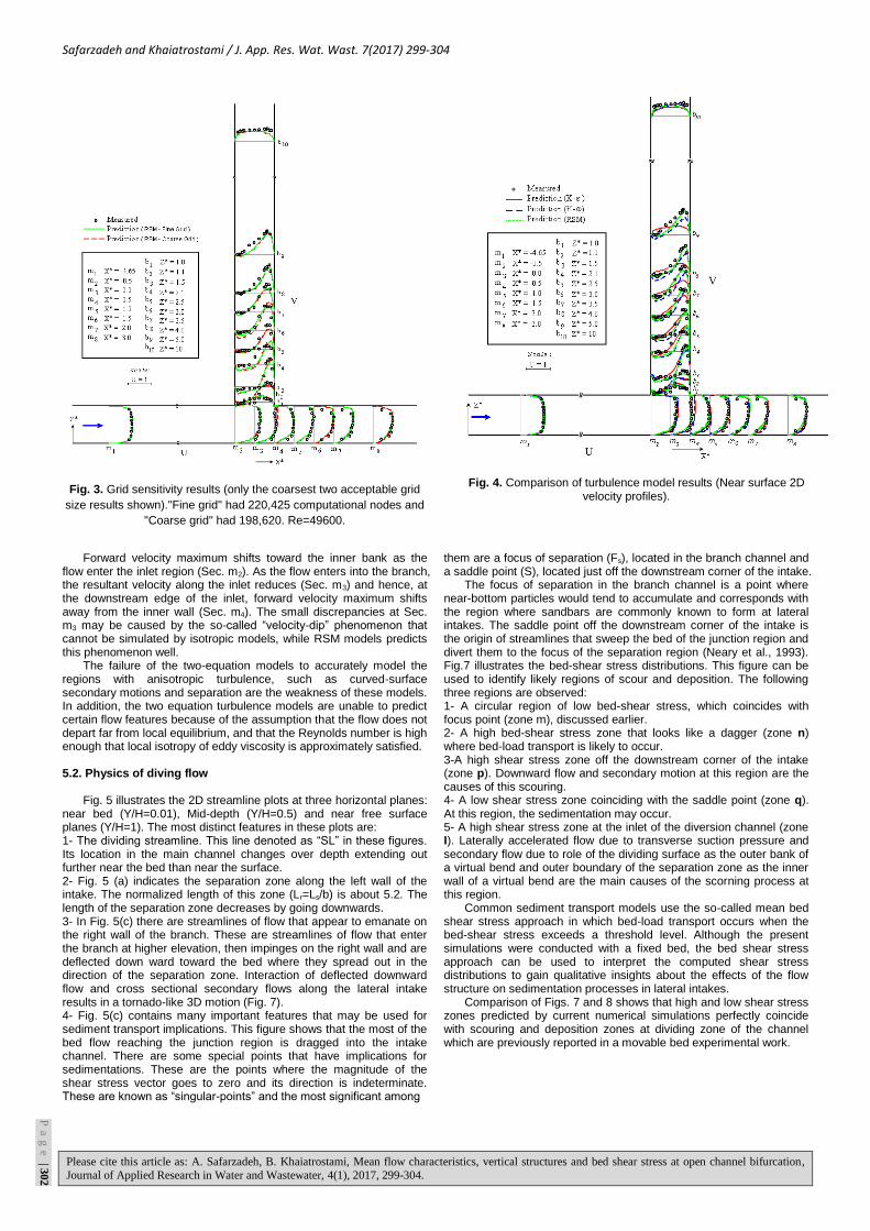
Fig. 5 illustrates the 2D streamline plots at three horizontal planes:

near bed (Y/H=0.01), Mid-depth (Y/H=0.5) and near free surface planes (Y/H=1). The most distinct features in these plots are: 1- The dividing streamline. This line denoted as “SL” in these figures. Its location in the main channel changes over depth extending out further near the bed than near the surface. 2- Fig. 5 (a) indicates the separation zone along the left wall of the intake. The normalized length of this zone (Lr=Ls/b) is about 5.2. The length of the separation zone decreases by going downwards. 3- In Fig. 5(c) there are streamlines of flow that appear to emanate on the right wall of the branch. These are streamlines of flow that enter the branch at higher elevation, then impinges on the right wall and are deflected down ward toward the bed where they spread out in the direction of the separation zone. Interaction of deflected downward flow and cross sectional secondary flows along the lateral intake results in a tornado-like 3D motion (Fig. 7). 4- Fig. 5(c) contains many important features that may be used for sediment transport implications. This figure shows that the most of the bed flow reaching the junction region is dragged into the intake channel. There are some special points that have implications for sedimentations. These are the points where the magnitude of the shear stress vector goes to zero and its direction is indeterminate. These are known as “singular-points” and the most significant among

them are a focus of separation (Fs), located in the branch channel and a saddle point (S), located just off the downstream corner of the intake.

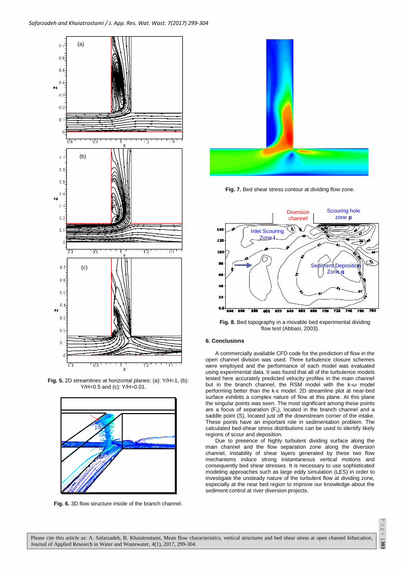
The focus of separation in the branch channel is a point where near-bottom particles would tend to accumulate and corresponds with the region where sandbars are commonly known to form at lateral intakes. The saddle point off the downstream corner of the intake is the origin of streamlines that sweep the bed of the junction region and divert them to the focus of the separation region (Neary et al., 1993). Fig.7 illustrates the bed-shear stress distributions. This figure can be used to identify likely regions of scour and deposition. The following three regions are observed: 1- A circular region of low bed-shear stress, which coincides with focus point (zone m), discussed earlier. 2- A high bed-shear stress zone that looks like a dagger (zone n) where bed-load transport is likely to occur. 3-A high shear stress zone off the downstream corner of the intake (zone p). Downward flow and secondary motion at this region are the causes of this scouring. 4- A low shear stress zone coinciding with the saddle point (zone q). At this region, the sedimentation may occur. 5- A high shear stress zone at the inlet of the diversion channel (zone I). Laterally accelerated flow due to transverse suction pressure and secondary flow due to role of the dividing surface as the outer bank of a virtual bend and outer boundary of the separation zone as the inner wall of a virtual bend are the main causes of the scorning process at this region.

Common sediment transport models use the so-called mean bed shear stress approach in which bed-load transport occurs when the bed-shear stress exceeds a threshold level. Although the present simulations were conducted with a fixed bed, the bed shear stress approach can be used to interpret the computed shear stress distributions to gain qualitative insights about the effects of the flow structure on sedimentation processes in lateral intakes.

Comparison of Figs. 7 and 8 shows that high and low shear stress zones predicted by current numerical simulations perfectly coincide with scouring and deposition zones at dividing zone of the channel which are previously reported in a movable bed experimental work.

Pa

ge

| 302




Fig. 5. 2D streamlines at horizontal planes: (a): Y/H=1, (b): Y/H=0.5 and (c): Y/H=0.01.

Fig. 6. 3D flow structure inside of the branch channel.

Fig. 7. Bed shear stress contour at dividing flow zone.

Fig. 8. Bed topography in a movable bed experimental dividing flow test (Abbasi, 2003).

6. Conclusions

A commercially available CFD code for the prediction of flow in the

open channel division was used. Three turbulence closure schemes were employed and the performance of each model was evaluated using experimental data. It was found that all of the turbulence models tested here accurately predicted velocity profiles in the main channel but in the branch channel, the RSM model with the k-ω model performing better than the k-ɛ model. 2D streamline plot at near-bed surface exhibits a complex nature of flow at this plane. At this plane the singular points was seen. The most significant among these points are a focus of separation (Fs), located in the branch channel and a saddle point (S), located just off the downstream corner of the intake. These points have an important role in sedimentation problem. The calculated bed-shear stress distributions can be used to identify likely regions of scour and deposition.

Due to presence of highly turbulent dividing surface along the main channel and the flow separation zone along the diversion channel, instability of shear layers generated by these two flow mechanisms induce strong instantaneous vertical motions and consequently bed shear stresses. It is necessary to use sophisticated modeling approaches such as large eddy simulation (LES) in order to investigate the unsteady nature of the turbulent flow at dividing zone, especially at the near bed region to improve our knowledge about the sediment control at river diversion projects.

(a)

(b)

(c)

Diversion channel

Scouring hole

zone p

Inlet Scouring

Zone I

Sediment Deposition Zone q

Pa

ge

| 303




References

Abbasi A., Experimental study of sediment control at lateral intake in straight channel, PhD Thesis, Tarbiat Modares University, (2003).

Barkdoll B., Sediment control at lateral diversion, PhD dissertation, University of Iowa, (1997).

Celik, I.B., Introductory turbulence modeling, Western Virginia University, (1999).

Fluent Inc., FLUENT user’s guide; Fluent, New Hampshire, (1993).

Gibson M.M., Launder B.E., Ground effects on pressure fluctuations in the atmospheric boundary layer, Journal of Fluid Mechanics 86 (1978) 491-511.

Launder B.E., Spalding D.B., Lectures in Mathematical Models of Turbulence, Academia press, London, England, (1972).

Launder B.E., Second-moment closure and its use in modeling turbulent industrial flows, International Journal of Numerical Methods in Fluids 9 (1989a) 963-985.

Launder B.E., Second-moment closure: present and future?, International Journal of Heat Fluid Flow 10 (1989b) 282-300.

Lien F.S., Leschziner M.A., Assessment of turbulent transport models including non-linear RNG eddy-viscosity formulation and second-moment closure, Computers and Fluids 23 (1994) 983-1004.

Neary V., Odgaard A.J., Three-dimensional flow structure at open channel diversions", Journal of Hydraulic Engineering 119 (1993) 1224–1230.

Neary V., Sotiropoulos F., Numerical investigation of laminar flows through 90-degree diversion of rectangular cross-section, Computer and Fluids 25 (1996) 95-118.

Shettar A., and Murthy K., A numerical study of division of flow in open channels, Journal of Hydraulic Research 34 (1996) 651-675.

Taylor E.H., Flow characteristics at rectangular open-channel junctions, Transactions of the American Society of Civil Engineers 109 (1944) 893–912.

Pa

ge

| 304

mean flow characteristics, vertical structures and bed shear stress at open channel...

Documents