mean shift tracking - freechateaut.free.fr/attachments/103_meanshift.pdf · mean shift tracking...

Mean Shift Tracking

CS4243 Computer Vision and Pattern Recognition

Leow Wee Kheng

Department of Computer ScienceSchool of Computing

National University of Singapore

(CS4243) Mean Shift Tracking 1 / 28

Mean Shift

Mean Shift

Mean Shift [Che98, FH75, Sil86]

An algorithm that iteratively shifts a data point to the average ofdata points in its neighborhood.

Similar to clustering.

Useful for clustering, mode seeking, probability density estimation,tracking, etc.


Mean Shift

Consider a set S of n data points xi in d-D Euclidean space X.

Let K(x) denote a kernel function that indicates how much x

contributes to the estimation of the mean.

Then, the sample mean m at x with kernel K is given by

m(x) =

n∑

i=1

K(x− xi)xi

n∑

i=1

K(x− xi)

(1)

The difference m(x)− x is called mean shift.

Mean shift algorithm: iteratively move date point to its mean.

In each iteration, x←m(x).

The algorithm stops when m(x) = x.


Mean Shift

The sequence x,m(x),m(m(x)), . . . is called the trajectory of x.

If sample means are computed at multiple points, then at eachiteration, update is done simultaneously to all these points.


Mean Shift Kernel

Kernel

Typically, kernel K is a function of ‖x‖2:

K(x) = k(‖x‖2) (2)

k is called the profile of K.

Properties of Profile:

1 k is nonnegative.

2 k is nonincreasing: k(x) ≥ k(y) if x < y.

3 k is piecewise continuous and

∫

∞

0k(x)dx <∞ (3)


Mean Shift Kernel

Examples of kernels [Che98]:

Flat kernel:

K(x) =

{

1 if ‖x‖ ≤ 10 otherwise

(4)

Gaussian kernel:K(x) = exp(−‖x‖2) (5)

(a) Flat kernel (b) Gaussian kernel


Mean Shift Density Estimation

Density Estimation

Kernel density estimation (Parzen window technique) is a popularmethod for estimating probability density[CRM00, CRM02, DH73].

For a set of n data points xi in d-D space, the kernel densityestimate with kernel K(x) (profile k(x)) and radius h is

f̃K(x) =1

nhd

n∑

i=1

K

(

x− xi

h

)

=1

nhd

n∑

i=1

k

(

∥

∥

∥

∥

x− xi

h

∥

∥

∥

∥

2)

(6)

The quality of kernel density estimator is measured by the meansquared error between the actual density and the estimate.



Mean squared error is minimized by the Epanechnikov kernel:

KE(x) =

1

2Cd

(d+ 2)(1− ‖x‖2) if ‖x‖ ≤ 1

0 otherwise(7)

where Cd is the volume of the unit d-D sphere, with profile

kE(x) =

1

2Cd

(d+ 2)(1− x) if 0 ≤ x ≤ 1

0 if x > 1(8)

A more commonly used kernel is Gaussian

K(x) =1

√

(2π)dexp

(

−1

2‖x‖2

)

(9)

with profile

k(x) =1

√

(2π)dexp

(

−1

2x

)

(10)



Define another kernel G(x) = g(‖x‖2) such that

g(x) = −k′(x) = −dk(x)

dx. (11)

Important Result

Mean shift with kernel G moves x along the direction of the gradient ofdensity estimate f̃ with kernel K.

Define density estimate with kernel K.

But, perform mean shift with kernel G.

Then, mean shift performs gradient ascent on density estimate.



Proof:

Define f̃ with kernel G

f̃G(x) ≡C

nhd

n∑

i=1

g

(

∥

∥

∥

∥

x− xi

h

∥

∥

∥

∥

2)

(12)

where C is a normalization constant.

Mean shift M with kernel G is

MG(x) ≡

n∑

i=1

g

(

∥

∥

∥

∥

x− xi

h

∥

∥

∥

∥

2)

xi

n∑

i=1

g

(

∥

∥

∥

∥

x− xi

h

∥

∥

∥

∥

2) − x (13)



Estimate of density gradient is the gradient of density estimate

∇̃fK(x) ≡ ∇f̃K(x)

=2

nhd+2

n∑

i=1

(x− xi) k′

(

∥

∥

∥

∥

x− xi

h

∥

∥

∥

∥

2)

=2

nhd+2

n∑

i=1

(xi − x) g

(

∥

∥

∥

∥

x− xi

h

∥

∥

∥

∥

2)

=2

Ch2f̃G(x)MG(x)

(14)

Then,

MG(x) =Ch2

2

∇̃fK(x)

f̃G(x)(15)

Thus, MG is an estimate of the normalized gradient of fK .

So, can use mean shift (Eq. 13) to obtain estimate of fK .


Mean Shift Tracking

Mean Shift Tracking

Basic Ideas [CRM00]:

Model object using color probability density.

Track target candidate in video by matching color probability oftarget with that of object model.

Use mean shift to estimate color probability and target location.


Mean Shift Tracking Object Model

Object Model

Let xi, i = 1, . . . , n, denote pixel locations of model centered at 0.

Represent color distribution by discrete m-bin color histogram.

Let b(xi) denote the color bin of the color at xi.

Assume size of model is normalized; so, kernel radius h = 1.

Then, probability q of color u, u = 1, . . . ,m, in object model is

qu = C

n∑

i=1

k(‖xi‖2) δ(b(xi)− u) (16)

C is the normalization constant

C =

[

n∑

i=1

k(‖xi‖2)]−1

(17)

Kernel profile k weights contribution by distance to centroid.


Mean Shift Tracking Object Model

δ is the Kronecker delta function

δ(a) =

{

1 if a = 00 otherwise

(18)

That is, contribute k(‖xi‖2) to qu if b(xi) = u.


Mean Shift Tracking Target Candidate

Target Candidate

Let yi, i = 1, . . . , nh, denote pixel locations of target centered at y.

Then, the probability p of color u in the target candidate is

pu(y) = Ch

nh∑

i=1

k

(

∥

∥

∥

∥

y − yi

h

∥

∥

∥

∥

2)

δ(b(yi)− u) (19)

Ch is the normalization constant

Ch =

[

nh∑

i=1

k

(

∥

∥

∥

∥

y − yi

h

∥

∥

∥

∥

2)]−1

(20)


Mean Shift Tracking Color Density Matching

Color Density Matching

Measure similarity between object model q and color p of target atlocation y.

Use Bhattacharyya coefficient ρ

ρ(p(y), q) =m∑

u=1

√

pu(y) qu (21)

ρ is the cosine of vectors (√p1, . . . ,

√pm)⊤ and (

√q1, . . . ,

√qm)⊤.

Large ρ means good color match.

Let y denote current target location with color probability{pu(y)}, pu(y) > 0 for u = 1, . . . ,m.

Let z denote estimated new target location near y, and colorprobability does not change drastically.


Mean Shift Tracking Color Density Matching

By Taylor’s series expansion

ρ(p(z), q) =1

2

m∑

u=1

√

pu(y) qu +1

2

m∑

u=1

pu(z)

√

qu

pu(y)(22)

Substitute Eq. 19 into Eq. 22 yields

ρ(p(z), q) =1

2

m∑

u=1

√

pu(y) qu +Ch

2

nh∑

i=1

wik

(

∥

∥

∥

∥

z− yi

h

∥

∥

∥

∥

2)

(23)

where weight wi is

wi =

m∑

u=1

δ(b(yi)− u)

√

qu

pu(y). (24)

To maximize ρ(p(z), q), need to maximize second term of Eq. 23.First term is independent of z.


Mean Shift Tracking Mean Shift Tracking Algorithm

Mean Shift Tracking Algorithm

Given {qu} of model and location y of target in previous frame:

(1) Initialize location of target in current frame as y.

(2) Compute {pu(y)}, u = 1, . . . ,m, and ρ(p(y), q).

(3) Compute weights wi, i = 1, . . . , nh.

(4) Apply mean shift: Compute new location z as

z =

nh∑

i=1

wi g

(

∥

∥

∥

∥

y − yi

h

∥

∥

∥

∥

2)

yi

nh∑

i=1

wi g

(

∥

∥

∥

∥

y − yi

h

∥

∥

∥

∥

2) (25)

where g(x) = −k′(x) (Eq. 11).(5) Compute {pu(z)}, u = 1, . . . ,m, and ρ(p(z), q).



(6) While ρ(p(z), q) < ρ(p(y), q), do z← 12(y + z).

(7) If ‖z− y‖ is small enough, stop.Else, set y← z and goto Step 1.

Notes:

Step 4: In practice, a window of pixels yi is considered.Size of window is related to h.

Step 6 is used to validate the target’s new location.Can stop Step 6 if y and z round off to the same pixel.

Tests show that Step 6 is needed only 0.1% of the time.

Step 7: Can stop algorithm if y and z round off to the same pixel.

To adapt to change of scale, can modify window radius h and letalgorithm converge to h that maximizes ρ(p(y, q)).



Example 1: Track football player no. 78 [CRM00].



Example 2: Track a passenger in train station [CRM00].


Mean Shift Tracking CAMSHIFT

CAMSHIFT

Mean Shift tracking uses fixed color distribution.

In some applications, color distribution can change, e.g., due torotation in depth.

Continuous Adaptive Mean Shift (CAMSHIFT) [Bra98]

Can handle dynamically changing color distribution.

Adapt Mean Shift search window size and compute colordistribution in search window.



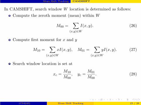
In CAMSHIFT, search window W location is determined as follows:

Compute the zeroth moment (mean) within W

M00 =∑

(x,y)∈W

I(x, y). (26)

Compute first moment for x and y

M10 =∑

(x,y)∈W

xI(x, y), M01 =∑

(x,y)∈W

yI(x, y). (27)

Search window location is set at

xc =M10

M00, yc =

M01

M00. (28)



CAMSHIFT Algorithm

(1) Choose the initial location of the search window.

(2) Perform Mean Shift tracking with revised method of setting searchwindow location.

(3) Store zeroth moment.

(4) Set search window size to a function of zeroth moment.

(5) Repeat Steps 2 and 4 until convergence.



Example 3: Track shirt with changing color distribution [AXJ03].


Reference

Reference I

J. G. Allen, R. Y. D. Xu, and J. S. Jin.Object tracking using camshift algorithm and multiple quantizedfeature spaces.In Proc. of Pan-Sydney Area Workshop on Visual Information

Processing VIP2003, 2003.

G. R. Bradski.Computer vision face tracking for use in a perceptual userinterface.Intel Technology Journal, 2nd Quarter, 1998.

Y. Cheng.Mean shift, mode seeking, and clustering.IEEE Trans. on Pattern Analysis and Machine Intelligence,17(8):790–799, 1998.


Reference

Reference II

D. Comaniciu, V. Ramesh, and P. Meer.Real-time tracking of non-rigid objects using mean shift.In IEEE Proc. on Computer Vision and Pattern Recognition, pages673–678, 2000.

D. Comaniciu, V. Ramesh, and P. Meer.Mean shift: A robust approach towards feature space analysis.IEEE Trans. on Pattern Analysis and Machine Intelligence,24(5):603–619, 2002.

R. O. Duda and P. E. Hart.Pattern Classification and Scene Analysis.Wiley, 1973.


Reference

Reference III

K. Fukunaga and L. D. Hostetler.The estimation of the gradient of a density function, withapplications in pattern recognition.IEEE Trans. on Information Theory, 21:32–40, 1975.

B. W. Silverman.Density Estimation for Statistics and Data Analysis.Chapman and Hall, 1986.


mean shift tracking - freechateaut.free.fr/attachments/103_meanshift.pdf · mean shift tracking...

Documents