mean value modelling of a poppet valve egr-system · mean value modelling of a poppet valve...
TRANSCRIPT
Mean value modelling of a poppet valveEGR-system
Master’s thesisperformed inVehicular Systems
byClaes Ericson
Reg nr: LiTH-ISY-EX-3543-2004
14th June 2004

Mean value modelling of a poppet valveEGR-system
Master’s thesis
performed inVehicular Systems,Dept. of Electrical Engineering
atLink opings universitet
by Claes Ericson
Reg nr: LiTH-ISY-EX-3543-2004
Supervisor:Jesper Ritzen, M.Sc.Scania CV AB
Mattias Nyberg, Ph.D.Scania CV AB
Johan Wahlstrom, M.Sc.Linkopings universitet
Examiner: Associate Professor Lars ErikssonLinkopings universitet
Linkoping, 14th June 2004

Avdelning, InstitutionDivision, Department
DatumDate
Sprak
Language
¤ Svenska/Swedish
¤ Engelska/English
¤
RapporttypReport category
¤ Licentiatavhandling
¤ Examensarbete
¤ C-uppsats
¤ D-uppsats
¤ Ovrig rapport
¤URL f or elektronisk version
ISBN
ISRN
Serietitel och serienummerTitle of series, numbering
ISSN
Titel
Title
ForfattareAuthor
SammanfattningAbstract
NyckelordKeywords
Because of new emission and on board diagnostics legislations, heavy truckmanufacturers are facing new challenges when it comes to improving the en-gines and the control software. Accurate and real time executable engine modelsare essential in this work. One successful way of lowering the NOx emissions isto use Exhaust Gas Recirculation (EGR). The objective of this thesis is to createa mean value model for Scania’s next generation EGR system consisting of apoppet valve and a two stage cooler. The model will be used to extend an exist-ing mean value engine model. Two models of different complexity for the EGRsystem have been validated with sufficient accuracy. Validation was performedduring static test bed conditions. The resulting flow models have mean relativeerrors of 5.0% and 9.1% respectively. The temperature model suggested has amean relative error of 0.77%.
Vehicular Systems,Dept. of Electrical Engineering581 83 Linkoping
14th June 2004
—
LITH-ISY-EX-3543-2004
—
http://www.vehicular.isy.liu.sehttp://www.ep.liu.se/exjobb/isy/2004/3543/
Mean value modelling of a poppet valve EGR-system
Medelvardesmodellering av EGR-system med tallriksventil
Claes Ericson
××
mean value engine modelling, EGR, poppet valve


Abstract
Because of new emission and on board diagnostics legislations, heavy truckmanufacturers are facing new challenges when it comes to improving the en-gines and the control software. Accurate and real time executable enginemodels are essential in this work. One successful way of lowering the NOxemissions is to use Exhaust Gas Recirculation (EGR). The objective of thisthesis is to create a mean value model for Scania’s next generation EGR sys-tem consisting of a poppet valve and a two stage cooler. The model will beused to extend an existing mean value engine model. Two models of differentcomplexity for the EGR system have been validated with sufficient accuracy.Validation was performed during static test bed conditions. The resultingflow models have mean relative errors of 5.0% and 9.1% respectively. Thetemperature model suggested has a mean relative error of 0.77%.
Keywords: mean value engine modelling, EGR, poppet valve
v
Outline
Chapter 1 describes the background and the objectives of the thesis.
Chapter 2 gives a description of the measurement setup and related prob-lems and also has a brief section on the working process.
Chapter 3 presents the existing model and modifications. The new EGRmodels are also introduced.
Chapter 4 describes the parameter tuning process.
Chapter 5 evaluates the EGR models using static measurements.
Chapter 6 discusses the results presented and possible future work.
Acknowledgment
First of all I would like to thank my supervisors Jesper Ritzen, Mattias Nybergand Johan Wahlstrom, and my examiner Lars Eriksson for many interestingand inspiring discussions during the work. Special thanks to Mikael Persson,NMEB and Mats Jennische, NEE for their support during the measurementsand to Manne Gustafson, NEE for advice regarding mean value modelling.Also thanks to all the other people at NE and NM who have contributed tomaking this thesis possible.
Claes EricsonSodertalje, June 2004
vi
Contents
Abstract v
Outline and Acknowledgment vi
1 Introduction 11.1 Background. . . . . . . . . . . . . . . . . . . . . . . . . . 1
1.1.1 Existing Work . . . . . . . . . . . . . . . . . . . . 21.2 Problem Formulation. . . . . . . . . . . . . . . . . . . . . 21.3 Objectives. . . . . . . . . . . . . . . . . . . . . . . . . . . 31.4 Delimitations . . . . . . . . . . . . . . . . . . . . . . . . . 31.5 Target Group . . . . . . . . . . . . . . . . . . . . . . . . . 3
2 Method 42.1 Working Process. . . . . . . . . . . . . . . . . . . . . . . 42.2 Measurements. . . . . . . . . . . . . . . . . . . . . . . . . 4
2.2.1 Measurement setup. . . . . . . . . . . . . . . . . . 52.2.2 Measured quantities. . . . . . . . . . . . . . . . . 52.2.3 Measurement problems. . . . . . . . . . . . . . . . 6
3 Modelling 93.1 Existing Model . . . . . . . . . . . . . . . . . . . . . . . . 9
3.1.1 Compressor. . . . . . . . . . . . . . . . . . . . . . 93.1.2 Intake Manifold. . . . . . . . . . . . . . . . . . . . 103.1.3 Engine . . . . . . . . . . . . . . . . . . . . . . . . 123.1.4 Exhaust Manifold. . . . . . . . . . . . . . . . . . . 143.1.5 Turbine . . . . . . . . . . . . . . . . . . . . . . . . 153.1.6 Turbine Shaft. . . . . . . . . . . . . . . . . . . . . 153.1.7 Exhaust System. . . . . . . . . . . . . . . . . . . . 15
3.2 EGR . . . . . . . . . . . . . . . . . . . . . . . . . . . . . . 163.2.1 Flow Model. . . . . . . . . . . . . . . . . . . . . . 163.2.2 Temperature Model. . . . . . . . . . . . . . . . . . 19
3.3 Extended Models. . . . . . . . . . . . . . . . . . . . . . . 21
vii
4 Tuning 234.1 Flow Model . . . . . . . . . . . . . . . . . . . . . . . . . . 23
4.1.1 Single restriction model. . . . . . . . . . . . . . . 234.1.2 Two stage restriction model. . . . . . . . . . . . . 25
4.2 Temperature model. . . . . . . . . . . . . . . . . . . . . . 264.2.1 Water cooler . . . . . . . . . . . . . . . . . . . . . 264.2.2 Air cooler. . . . . . . . . . . . . . . . . . . . . . . 28
5 Validation 295.1 Flow Model . . . . . . . . . . . . . . . . . . . . . . . . . . 29
5.1.1 Single restriction model. . . . . . . . . . . . . . . 295.1.2 Two stage restriction model. . . . . . . . . . . . . 31
5.2 Temperature Model. . . . . . . . . . . . . . . . . . . . . . 315.2.1 Water cooler . . . . . . . . . . . . . . . . . . . . . 325.2.2 Air cooler. . . . . . . . . . . . . . . . . . . . . . . 33
5.3 Sensitivity analysis. . . . . . . . . . . . . . . . . . . . . . 345.3.1 Water cooler fouling. . . . . . . . . . . . . . . . . 36
5.4 Summary . . . . . . . . . . . . . . . . . . . . . . . . . . . 37
6 Conclusions and Future Work 386.1 Conclusions. . . . . . . . . . . . . . . . . . . . . . . . . . 386.2 Future Work. . . . . . . . . . . . . . . . . . . . . . . . . . 38
References 40
Notation 42
viii
Chapter 1
Introduction
This master’s thesis was performed at Scania CV AB in Sodertalje. Scania isa worldwide manufacturer of heavy duty trucks, buses and engines for marineand industrial use. The work was carried out at the engine software develop-ment department, which is responsible for the engine control and the on boarddiagnostics (OBD) software.
1.1 Background
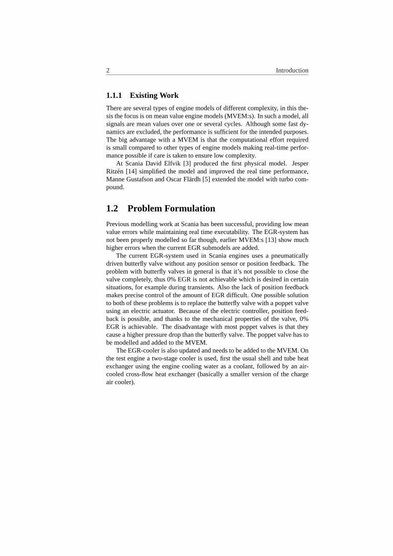
Because of new emissions legislation, both within the European Union andthe United States, heavy truck manufacturers are facing new challenges whenit comes to improving the engines and the control software. Besides the re-quirements of substantially lowered emissions, new legislation such as Euro4 and 5 also requires advanced On Board Diagnostics (OBD) systems. TheOBD system has to meet certain demands, for example faults resulting inemission levels higher than the legislative limits must be detected.
In order to meet these goals, it is important to have models of the enginewith sufficient accuracy. The models are used for improved model basedcontrol and for model based diagnosis.
One successful way of lowering the NOx emissions is to use Exhaust GasRecirculation (EGR). This means that some of the exhaust gas is circulatedback into the intake manifold. The amount of NOx emissions produced dur-ing the combustion is closely related to the peak temperature. By reducing theamount of fresh air in the intake manifold and replacing it with exhaust gas, alower peak temperature during combustion is achieved resulting in decreasedNOx. In order to be able to inject the exhaust gas into the intake manifold, itmust have a sufficiently high pressure. This can be achieved in several ways,for example by using a venturi, turbo compound or as used in this thesis; avariable geometry turbocharger (VGT). By adjusting the vanes in the VGT ahigh exhaust pressure is achieved.
1
2 Introduction
1.1.1 Existing Work
There are several types of engine models of different complexity, in this the-sis the focus is on mean value engine models (MVEM:s). In such a model, allsignals are mean values over one or several cycles. Although some fast dy-namics are excluded, the performance is sufficient for the intended purposes.The big advantage with a MVEM is that the computational effort requiredis small compared to other types of engine models making real-time perfor-mance possible if care is taken to ensure low complexity.
At Scania David Elfvik [3] produced the first physical model. JesperRitzen [14] simplified the model and improved the real time performance,Manne Gustafson and Oscar Flardh [5] extended the model with turbo com-pound.
1.2 Problem Formulation
Previous modelling work at Scania has been successful, providing low meanvalue errors while maintaining real time executability. The EGR-system hasnot been properly modelled so far though, earlier MVEM:s [13] show muchhigher errors when the current EGR submodels are added.
The current EGR-system used in Scania engines uses a pneumaticallydriven butterfly valve without any position sensor or position feedback. Theproblem with butterfly valves in general is that it’s not possible to close thevalve completely, thus 0% EGR is not achievable which is desired in certainsituations, for example during transients. Also the lack of position feedbackmakes precise control of the amount of EGR difficult. One possible solutionto both of these problems is to replace the butterfly valve with a poppet valveusing an electric actuator. Because of the electric controller, position feed-back is possible, and thanks to the mechanical properties of the valve, 0%EGR is achievable. The disadvantage with most poppet valves is that theycause a higher pressure drop than the butterfly valve. The poppet valve has tobe modelled and added to the MVEM.
The EGR-cooler is also updated and needs to be added to the MVEM. Onthe test engine a two-stage cooler is used, first the usual shell and tube heatexchanger using the engine cooling water as a coolant, followed by an air-cooled cross-flow heat exchanger (basically a smaller version of the chargeair cooler).
1.3. Objectives 3
1.3 Objectives
The objectives of this thesis is to create a mean value model for the new EGRsystem consisting of a poppet valve and a two stage EGR-cooler. The modelshould be:
• Physical
• Accurate
• Modular
1.4 Delimitations
The exhaust brake that the engine is equipped with is not modeled. Duringcalibration and validation, the exhaust brake has not been active.
1.5 Target Group
The target group of this work is primarily employees at Scania CV and M.Sc./B.Sc.students with basic knowledge in vehicular systems and thermodynamics.
Chapter 2
Method
In this chapter the working process will be described briefly, and the mea-surements will be described.
2.1 Working Process
Theoretical studies First of all earlier works such as masters theses, articlesand books related to engine modelling were studied in addition to somethermodynamics and fluid mechanics.
Modelling Physically and/or empirically based models were developed andimplemented in Matlab/Simulink.
Measurement Measurements were planned and performed in an engine testbed.
Tuning The parameters in the earlier developed models were tuned using theoptimization software Lsoptim [4].
Validation Using a set of data separate from the one used during parametersetting measured outputs are compared with simulated outputs.
The modelling and parameter setting parts were reworked many timesduring the course of work after measurements had shown limitations in earlierversions of the models.
2.2 Measurements
All measurements were performed in an engine test bed. In the test bed con-figuration the engine is equipped with many temperature and pressure sensorsin addition to the production sensors.
4
2.2. Measurements 5
2.2.1 Measurement setup
Measurements were performed both at steady state and continuous condi-tions. Some of the sensors have very slow dynamics however, so care had tobe taken in order not to misinterpret the resulting data. During steady statemeasurements there is a stabilization phase of 30 seconds and after that thesoftware calculates a mean value of the variables for another 30 seconds. Con-tinuous measurements were performed at a sampling rate of 10Hz. For datacollection the standard measurement system of the test bed was used mostof the time. In order to validate some of the measurements, the ATI Visionmeasurement system was used.
2.2.2 Measured quantities
Temperatures are measured using 5mm pt-100 temperature sensors. The 5mmdiameter of the sensors makes them very ”bulletproof” and capable of with-standing high temperatures, but on the other hand makes them quite slow.However, during steady state measurements this is not an issue. When usingATI Vision, 3mm K-elements were used instead (because of the lack of inputsfor pt-100 sensors). For pressure measurements, the standard sensors of thetest bed were used. All pressure sensors are mounted perpendicular to theflow and consequently it is the static pressure that is measured.
The position of the poppet valve was measured using the built in positionsensor of the Eaton valve. The output of this sensor is an analogue signalbetween 0 and 5 volts, directly proportional to the valve lift.
The position of the vanes in the VGT was measured using the built inposition sensor of the Holset turbocharger. The output of this sensor is ananalogue signal between 0 and 5 volts.
A flange manufactured by Holset was used to determine the air flow intothe engine. The sensor is installed a couple of meters before the intake, whichmakes it unusable for dynamic measurements but ok for steady state.
The gas flow through the EGR system was determined using an EGR ratevariable calculated in the test bed computer. The variable is calculated by thecomparison of theCO2 rate in the intake manifold with theCO2 rate in theexhaust gas using a HORIBA exhaust gas analyzing system. The fact thatthe exhaust gases (which are led through pipes to the adjacent room wherethe analyzing system is located) are used to determine the EGR rate impliesa delay of several seconds making it usable only in steady state.
6 Chapter 2. Method
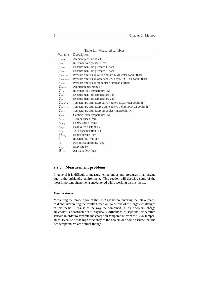
Table 2.1:Measured variablesVariable Descriptionpamb Ambient pressure [bar]pim Inlet manifold pressure [bar]pem1 Exhaust manifold pressure 1 [bar]pem2 Exhaust manifold pressure 2 [bar]pavalve Pressure after EGR valve / before EGR water cooler [bar]pawater Pressure after EGR water cooler / before EGR air cooler [bar]paair Pressure after EGR air cooler / intercooler [bar]Tamb Ambient temperature [K]Tim Inlet manifold temperature [K]Tem1 Exhaust manifold temperature 1 [K]Tem2 Exhaust manifold temperature 2 [K]Tavalve Temperature after EGR valve / before EGR water cooler [K]Tawater Temperature after EGR water cooler / before EGR air cooler [K]Taair Temperature after EGR air cooler / intercooler[K]Tcool Cooling water temperature [K]ntrb Turbine speed [rpm]neng Engine speed [rpm]uegr EGR valve position [V]uvgt VGT vane position [V]Meng Engine torque [Nm]δ Injected fuel [mg/inj]α Fuel injection timing [deg]xegr EGR rate [%]Wair Air mass flow [kg/s]
2.2.3 Measurement problems
In general it is difficult to measure temperatures and pressures in an enginedue to the unfriendly environment. This section will describe some of themost important phenomena encountered while working on this thesis.
Temperatures
Measuring the temperature of the EGR gas before entering the intake mani-fold and interpreting the results turned out to be one of the largest challengesof this thesis. Because of the way the combined EGR air cooler / chargeair cooler is constructed it is physically difficult to fit separate temperaturesensors in order to separate the charge air temperature from the EGR temper-ature. Because of the high efficiency of the coolers one could assume that thetwo temperatures are similar though.
2.2. Measurements 7
The real problem turned out to be the temperatures reported by theTaair
temperature sensor. With an ambient temperature of 298K,Taair reported290K during certain conditions. This is physically impossible since the coolercannot cool the gases to a lower temperature than ambient. That would in-dicate an efficiency of more than 100%. The temperature sensors used werecalibrated and found to be working properly.
There is a reasonable explanation for these low temperatures however.The exhaust gas contains large amounts of water which could cling onto thetemperature sensor in the form of droplets, then evaporate while cooling downthe temperature sensor, which in return reports a temperature unrepresenta-tive of the gas temperature. The fact that a wet thermometer reports a lowertemperature than a dry is used in for example psychrometers [2]. Compar-ing Taair with the temperature in the intake manifoldTim shows that thetemperature of the gas mixture increases by approximately 5 degrees on av-erage, which is what we expect due to heat transfer from the engine block.A five degree increase still means that the temperature in the intake manifoldis lower than ambient temperature in some points. The difference is slightduring most temperature conditions though and the wet thermometer theorycould still hold. One basic problem when measuring such low temperaturesis that a difference of a few degrees results in physically impossible results.With the previous EGR systems this was never an issue because the temper-atures were much higher, often in the 350-400K region where a two-degreedifference is negligible. In order to bring clarity to the situation, anothermeasurement system, ATI vision, with 3mm K-element temperature sensorsin place of the pt-100:s was used. The sub-ambient temperatures were notobserved with this setup. Possibly the effect of water droplets on the temper-ature sensor was smaller due to the smaller diameter. These measurementsdid confirm the first suspicion that the temperature sensor did not measurewhat was intended, rather than the theory that a new unexplained physicalphenomena had been discovered. Using measurement data which could notbe fully trusted did impose problems while modelling the EGR air cooler asfurther discussed in chapter3.2.2.
Another issue when it came to measuring problems wasTawater, the tem-perature after the EGR water cooler. In several points during low EGR flows,this temperature was substantially lower thanTcool, once again indicatingan efficiency of over 100%. There are two possible explanations for thisphenomena. The temperature sensor could be cooled down because of heattransfer from surrounding pipe walls because of the extremely low flow, re-sulting in an output more representative of wall temperature than gas temper-ature. The other theory is that fresh air from the charge air cooler was leakingbackwards through the EGR system under these operating conditions, mean-ing thatTawater was actually measuring the temperature of an exhaust gas /charge air mixture.
8 Chapter 2. Method
Pressures
One problem in general with the type of pressure sensors used and mean valuetype of measuring is that the sensors does not capture the high frequencypressure pulsations originating from the opening and closing of exhaust andinlet valves. Looking at older measurements performed at Scania, this isespecially apparent in the exhaust manifold pressure.
The pressure sensor located after the poppet valve,pavalve, is likely togive less than optimal results due to turbulence after the valve and the poorphysical location. One indication of this is that the pressure reported fromthe sensor is lower than the pressure in the intake manifold in many operatingconditions, thus indicating a pressure increase over the EGR coolers, whichis physically impossible. Looking atpawater, which is better located along astraight pipe, also shows a lower pressure thanpim in many points, leadingus to believe that there is another explanation than measurement problems.The previously discussed pressure pulsations could be one such explanation.These pulsations will drive a flow through the EGR-system even if the staticpressures indicate a flow in the opposite direction.
Chapter 3
Modelling
This chapter describes the modelling of the components in the turbochargeddiesel engine. Some of the components in the existing model are modified towork properly with the new components and the model is extended with VGTand EGR.
3.1 Existing Model
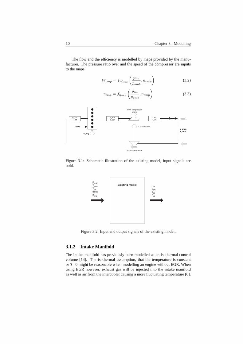
In this section, the existing mean value engine model at Scania will be de-scribed briefly. The model is for a turbocharged diesel engine without turbocompound and exhaust brake. It has been developed in several steps by com-bining submodels earlier presented in the master’s theses [15] [13], enginemodelling literature [8] and others [7]. The final steps in the developmentof the model was taken by David Elfvik [3] and Jesper Ritzen [14] in theirmaster’s theses. The different submodels will be presented following theair/exhaust path through the engine, starting from the intake side. An illustra-tion of the model can be found in figure3.1and the inputs and outputs can beseen in figure3.2.
3.1.1 Compressor
The first component in the air path that is modelled is the compressor, whichis stiffly connected to the turbine via the turbine shaft. The modelling of theturbine and the turbine shaft is presented in section3.1.5and3.1.6. Earlier,this model has been presented in [7]. Two output signals are of interest; thetorque produced by the compressor and the mass flow through the compres-sor. The torque is given by:
τcmp =WcmpcpairTamb
ηcmpωcmp
(pim
pamb
) γair−1γair − 1
(3.1)
9
10 Chapter 3. Modelling
The flow and the efficiency is modelled by maps provided by the manu-facturer. The pressure ratio over and the speed of the compressor are inputsto the maps.
Wcmp = fWcmp
(pim
pamb, ncmp
)(3.2)
ηcmp = fηcmp
(pim
pamb, ncmp
)(3.3)
p_em, T_em
p_im, T_im
n_compressor
Flow compressor tubine
Flow compressor
p_amb, T_amb
p_es, T_es
n_eng
delta
Figure 3.1: Schematic illustration of the existing model, input signals arebold.
Existing model p amb T amb T im delta n eng
p im p em p es n trb
Figure 3.2:Input and output signals of the existing model.
3.1.2 Intake Manifold
The intake manifold has previously been modelled as an isothermal controlvolume [14]. The isothermal assumption, that the temperature is constantor T=0 might be reasonable when modelling an engine without EGR. Whenusing EGR however, exhaust gas will be injected into the intake manifoldas well as air from the intercooler causing a more fluctuating temperature [6].
3.1. Existing Model 11
ThusT must be taken into account. Heat transfer between the intake manifoldwalls and the air mixture is not taken into account. Because of the air cooler,the temperatures involved are not higher than for a non-EGR engine, thus theaddition of the EGR-system does not motivate a change. The volume andtemperature in the intake manifold is identical for the exhaust gas and air.Differentiating the ideal gas law:
˙pim = ˙pexh + ˙pair =
mexhRexhTexh
Vim+
mexhRexhTexh
Vim+
mairRairTair
Vim+
mairRairTair
Vim=
WegrRexhTexh
Vim+
WcacRairTair
Vim− Weng,inRimTim
Vim+
+mexhRexhTexh
Vim+
mairRairTair
Vim(3.4)
The internal energy of an ideal gas, assuming thatcv is constant:
Uexh = mexhuexh = mexhcv,exhTexh
(3.5)
Differentiate:
dUexh
dt= mexhcv,exhTexh + mexhcv,exhTexh =
Wegrcv,exhTexh − xegrWeng,incv,imTim + mexhcv,exhTexh
(3.6)
Energy conservation for an open system gives:
dUexh
dt= Hexh,in − Hexh,out − Q (3.7)
whereHexh,in = Wegrcp,exhTexh (3.8)
andHexh,out = xegrWeng,incp,exhTexh (3.9)
wherexegr =
mexh
mair + mexh(3.10)
also, if heat transfer is neglected,Q = 0. Combining3.6and3.7:
Texh =1
mexhcv,exh(WegrTexhRexh − xegrWeng,inRimTim) (3.11)
12 Chapter 3. Modelling
Equations3.5through3.11can be derived analogously for the air fraction.Combining3.4with 3.11(and its air counterpart):
pim =Wegr
Vim
(RexhTexh − R2
exh
cv,exhTexh
)+
Wcac
Vim
(RairTair − R2
air
cv,airTair
)−
Weng,in
Vim
(RimTim − Rexh
cv,exhxegrRimTim − Rair
cv,air(1− xegr)RimTim
)=
1Vim
(WegrRexhγexhTexh + WcacRairγairTair −Weng,inRimγimTim)
(3.12)
This relation is often referred to as an adiabatic control volume. Thestates chosen are pressure and the mass in the intake manifold separated intoexhaust gas and air. Another possibility would be to include a temperaturestate and exclude the mass states. The advantage using mass states is that theEGR-rate can be easily calculated according to3.10.
The temperature in the intake manifold can be calculated using the idealgas law:
Tim =pimVim
(mexh + mair)Rim(3.13)
Summarizing the Intake Manifold model:
pim =1
Vim(RairγairWcacTcac + RexhγexhWegrTegr
−RimγimWeng,inTim) (3.14)
mexh = Wegr − xegrWeng,in (3.15)
mair = Wcac − (1− xegr)Weng,in (3.16)
3.1.3 Engine
The engine submodel consists of two submodels, one for the flow through theengine and one for the temperature of the exhaust gases.
Engine Flow Model
During the intake phase of the cylinder cycle, air fills the cylinders. The airmass-flow into the engine depends on many different factors, but the mostimportant are engine speed, intake manifold pressure and temperature. Vol-umetric efficiency,ηvol, is the ratio between the volume inducted into theengine and the volume ideally inducted (the displaced volume every cylindercycle). The density is assumed to be the same in the intake manifold as in thecylinders during the intake phase, therefore the volumetric efficiency is also
3.1. Existing Model 13
the ratio between actual and ideally inducted mass. The air mass flow into theengine is ideally:
mideal =Vdnengpim
2RTim(3.17)
Consequently the actual amount inducted into the engine is:
m = ηvolVdnengpim
2RTim(3.18)
Previously a volumetric efficiency model has been used which is based ona look-up table with engine speed and intake manifold temperature as inputs:
ηvol = fηvol(neng, Tim) (3.19)
In this thesis another model, presented in [16] has been used with goodperformance:
ηvol = Cvol
rc −(
pem
pim
)1/γair
rc − 1(3.20)
whererc is the compression ratio andCvol is a constant.
During the exhaust phase, the exhaust gases are pressed out of the cylinderand into the exhaust manifold. The flow out of the engine equals the sum ofthe flow into the engine and the amount of fuel injected.
Wengout = Wengin + Wfuel, (3.21)
where
Wfuel =δnengNcyl
120(3.22)
Exhaust Gas Temperature
Two different models for the exhaust gas temperature have previously beenused at Scania. In the first one the exhaust gas temperature is modelled as anideal Otto cycle, earlier presented in [15]. A non-linear equation system hasto be solved in every time step. The equations are:
Tem = T1
(pem
pim
) γexh−1γexh
(1 +
qin
cvT1rcγexh−1
) 1γexh
(3.23)
The specific energy of the charge per mass is:
qin =WfuelqHV
WengIn + Wfuel(1− xr). (3.24)
14 Chapter 3. Modelling
The residual gas fraction is:
xr =1rc
(pem
pim
) 1γexh
(1 +
qin
cvT1rcγexh−1
)− 1γexh
(3.25)
The model is complete with:
T1 = xrTem + (1− xr)Tim. (3.26)
The problem with this model is the poor performance during low load condi-tions, that is whenWfuel is small.
The second model used is a static model, presented in [12]. The equationis:
Tem = Tim +QLHV h(Wfuel, NEng)
cp,exh(Weng,in + Wfuel)(3.27)
h(Wfuel, NEng) is a look-up table. This model will neglect some dynamics,but has proven to be a better overall choice.
An improved model for the exhaust gas temperature would be desirable,but this is beyond the scope of this thesis.
3.1.4 Exhaust Manifold
The exhaust manifold is modelled as an isothermal control volume, that is bydifferentiating the ideal gas law and neglectingT . Why is it reasonable toassume thatT is negligible in this case? Compared to the intake manifoldthere is only one flow into the exhaust manifold, thus there will be no mixingof gases with different temperatures, flows and thermodynamic properties asin the case with the intake manifold. The fact that a second outward flow forthe EGR system is added doesn’t change the temperature properties of theexhaust manifold compared to earlier non-EGR MVEM:s [14] presented atScania. The inward flow is equal to the flow out of the engine and the outwardflow is the flow through the turbine plus the flow through the EGR-valve.
Win = Wengout (3.28)
Wout = Wtrb + Wegr (3.29)
The model for the exhaust manifold will contain one state only with asingle parameterVem:
pem =RexhTem(Wengout −Wtrb −Wegr)
Vem(3.30)
3.1. Existing Model 15
3.1.5 Turbine
The turbine is modelled analogously to the compressor, however since theturbocharger has a variable geometry, the control signaluvgt also comes intoplay.
The torque equation is essentially the same as for the compressor, but forexpanding instead of compressing the gas. The torque is given by:
τtrb =Wtrbcpexh
Temηtrb
ωtrb
1−
(pem
pes
) 1−γexhγexh
(3.31)
As for the compressor, the mass flow and efficiency are modelled by mapsprovided by the manufacturer.
Wtrb = fWtrb
(pem
pes, ntrb, uvgt
)(3.32)
ηtrb = fηtrb
(pem
pes, ntrb, uvgt
)(3.33)
The temperature after the turbine is modelled as:
Ttrbout =(
1 + ηtrb
((pem
pes
) 1−γexhγexh − 1
))Tem (3.34)
3.1.6 Turbine Shaft
The turbine shaft connects the turbine and the compressor. By use of New-ton´s second law the derivative of the turbine shaft speed can be modelledas:
ωtrb =1
Jtrb(τtrb − τcmp) (3.35)
The same approach has previously been used in for example [7] and [13].
3.1.7 Exhaust System
As above, the pressure is modelled using a standard control volume, assumingthe temperature variations are slow. The flow into the volume equals the flowthrough the turbine and the flow out of the volume equals the flow throughthe exhaust pipe.
pes =RexhTes
Ves(Wtrb −Wes) (3.36)
The flow out of the volume is modelled using a quadratic restriction, withthe restriction constantkes [1]:
16 Chapter 3. Modelling
W 2es =
pes
kesRexhTes(pes − pamb) (3.37)
The parameterskes adVes are estimated from measurement data.
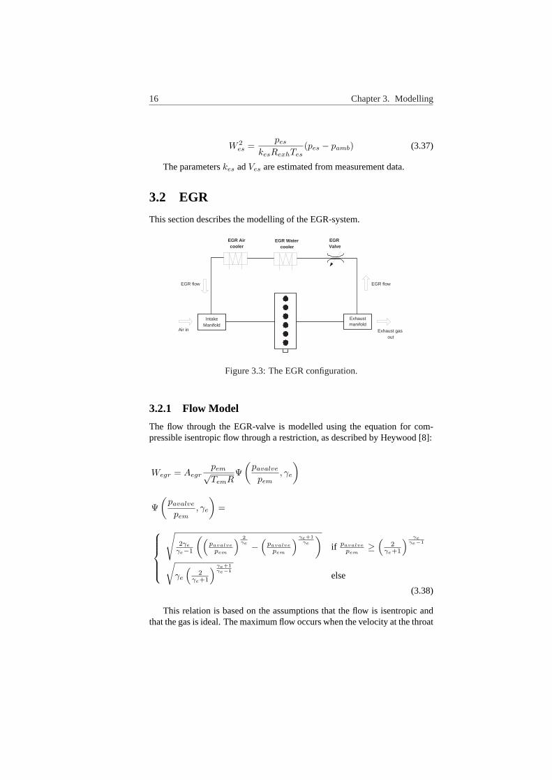
3.2 EGR
This section describes the modelling of the EGR-system.
Exhaust manifold
Intake Manifold
EGR Air cooler
EGR Water cooler
EGR Valve
EGR flow
Exhaust gas out
EGR flow
Air in
Figure 3.3:The EGR configuration.
3.2.1 Flow Model
The flow through the EGR-valve is modelled using the equation for com-pressible isentropic flow through a restriction, as described by Heywood [8]:
Wegr = Aegrpem√TemR
Ψ(
pavalve
pem, γe
)
Ψ(
pavalve
pem, γe
)=
√2γe
γe−1
((pavalve
pem
) 2γe −
(pavalve
pem
) γe+1γe
)if pavalve
pem≥
(2
γe+1
) γeγe−1
√γe
(2
γe+1
) γe+1γe−1
else
(3.38)
This relation is based on the assumptions that the flow is isentropic andthat the gas is ideal. The maximum flow occurs when the velocity at the throat
3.2. EGR 17
equals the velocity of sound which occurs at the critical pressure ratio
pavalve
pem=
(2
γe + 1
) γeγe−1
(3.39)
Aegr is the effective flow area of the EGR valve. In the ideal caseAegr
for a poppet valve is a function of valve lift only:
Aegr = k1 + k2uegr + k3u2egr (3.40)
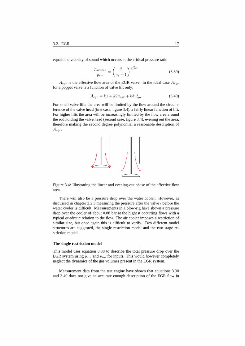
For small valve lifts the area will be limited by the flow around the circum-ference of the valve head (first case, figure3.4), a fairly linear function of lift.For higher lifts the area will be increasingly limited by the flow area aroundthe rod holding the valve head (second case, figure3.4), evening out the area,therefore making the second degree polynomial a reasonable description ofAegr.
Figure 3.4:Illustrating the linear and evening-out phase of the effective flowarea.
There will also be a pressure drop over the water cooler. However, asdiscussed in chapter2.2.3measuring the pressure after the valve / before thewater cooler is difficult. Measurements in a blow-rig have shown a pressuredrop over the cooler of about 0.08 bar at the highest occurring flows with atypical quadratic relation to the flow. The air cooler imposes a restriction ofsimilar size, but once again this is difficult to verify. Two different modelstructures are suggested, the single restriction model and the two stage re-striction model.
The single restriction model
This model uses equation3.38 to describe the total pressure drop over theEGR system usingpem andpim for inputs. This would however completelyneglect the dynamics of the gas volumes present in the EGR system.
Measurement data from the test engine have shown that equations3.38and3.40 does not give an accurate enough description of the EGR flow in
18 Chapter 3. Modelling
the single restriction model. There are two different options which couldexplain this phenomena. Either the measurements are incorrect or the modelstructure / choice of inputs to the model is at fault. As discussed in chapter2.2.3, pressure pulsations in the exhaust manifold could be one explanation.Ricardo consulting [10] suggested that the pulsations could be accounted forby using an additive compensation factor on the exhaust pressure in the formof a two-dimensional look-up table using engine speed and load as inputs:
pem,comp = pem + h(n, δ) (3.41)
To test this concept the desired exhaust pressure, that is the pressure whichwould give a perfect match to measured EGR flow assuming an effective flowarea according to equation3.40, was calculated backwards from equation3.38using measurement data. However, no signs were visible that the dif-ference between desired and actual exhaust pressure is correlated to neitherload nor engine speed. Another possibility would be to use a black-box typeof compensation factor on the effective flow area:
Aegr,comp = f(pem, pim, Uegr)Aegr (3.42)
Looking at measurement data there is a connection between pressure quotientover the valve and diverging calculated effective flow areas. For a given valveposition, the lower the pressure quotient, the higher the calculated effectiveflow area. Taking another look at the measurement data it was noted that forhigh valve lifts not only the pressure quotient, but also the absolute pressurehas an effect on calculatedAegr. Increasing exhaust pressure with identicalpressure quotient results in a larger calculated effective flow area. Thereforethe following relation for the effective flow area is suggested:
Aegr,comp = (pim
pem)a1(a2 + Uegrp
a3em)Aegr (3.43)
where a1, a2 and a3 are constants.
The polynomial version of the effective flow area as well as the black-boxcompensated version will be evaluated further in chapter4.1.
The two stage restriction model
Another option is to ignore the pressure measurementspavalve andpawater
and introduce one quadratic restriction for both coolers:
Wegr,out =√
pavalve
k1RexhTawater(pavalve − pim + k2) (3.44)
wherek1 is the restriction constant andk2 is a compensation constant forpressure pulsations.k1 andk2 will be calculated to optimize the overall per-formance of the flow through the EGR system. An isothermal control volume
3.2. EGR 19
is introduced between the EGR valve restriction and the cooler restriction inorder to model the dynamics:
pavalve =RexhTavalve
Vegr(Wegr −Wegr,out) (3.45)
whereVegr is a constant. The temperature after the water cooler is used tocalculate the density in the quadratic restriction. This is one of several choicesthat could be made, the reason this choice was made is that this temperatureis somewhat an average of the temperature in the EGR system.
The single restriction and two stage restriction models will be comparedfurther in chapter4.1.
3.2.2 Temperature Model
There will be a slight temperature difference over the valve. One possiblemodel is based on isentropic compression:
Tavalve = (pavalve
pem)
γ−1γ Tem (3.46)
In reality however, it was difficult to measure the temperature after the valve,making validation very difficult. Especially during low gas flows in the EGRsystem the temperature diverge from physically reasonable values, probablydue to heat transfer from the surrounding walls. Either way the temperaturedrop will be slight, less than 20 degrees in most cases which will not affectthe temperature after the EGR-coolers significantly. Therefore no tempera-ture model for the valve is included, making the temperature after the valveidentical with the exhaust manifold temperature in the model.
The cooling of the EGR gas is made by a two-stage cooler, first the stan-dard heat exchanger using the engine cooling water as coolant and secondlyan air cooler. The heat exchanger effectiveness is defined as:
ε =actual heat transfer
maximum possible heat transfer(3.47)
or equivalently
ε =∆T(minimum fluid)
Maximum temperature difference in heat exchanger(3.48)
The minimum fluid is the one experiencing the largest temperature differenceover the heat exchanger. Assuming that the coolant has the lower temperaturedrop (this is normally the case)3.48can be rewritten as:
Tout = Tin + ε(Tcool − Tin) (3.49)
20 Chapter 3. Modelling
One way of describing the efficiency is the effectiveness-NTU method.NTU is short for number of transfer units:
N =UA
Cmin(3.50)
where U is the overall heat transfer coefficient, A is the effective area andCmin = mcp of the minimum fluid. Thus, NTU is indicative of the size ofthe heat exchanger. Holman [9] has listed the efficiencies as a function ofNTU for various types of heat exchangers.
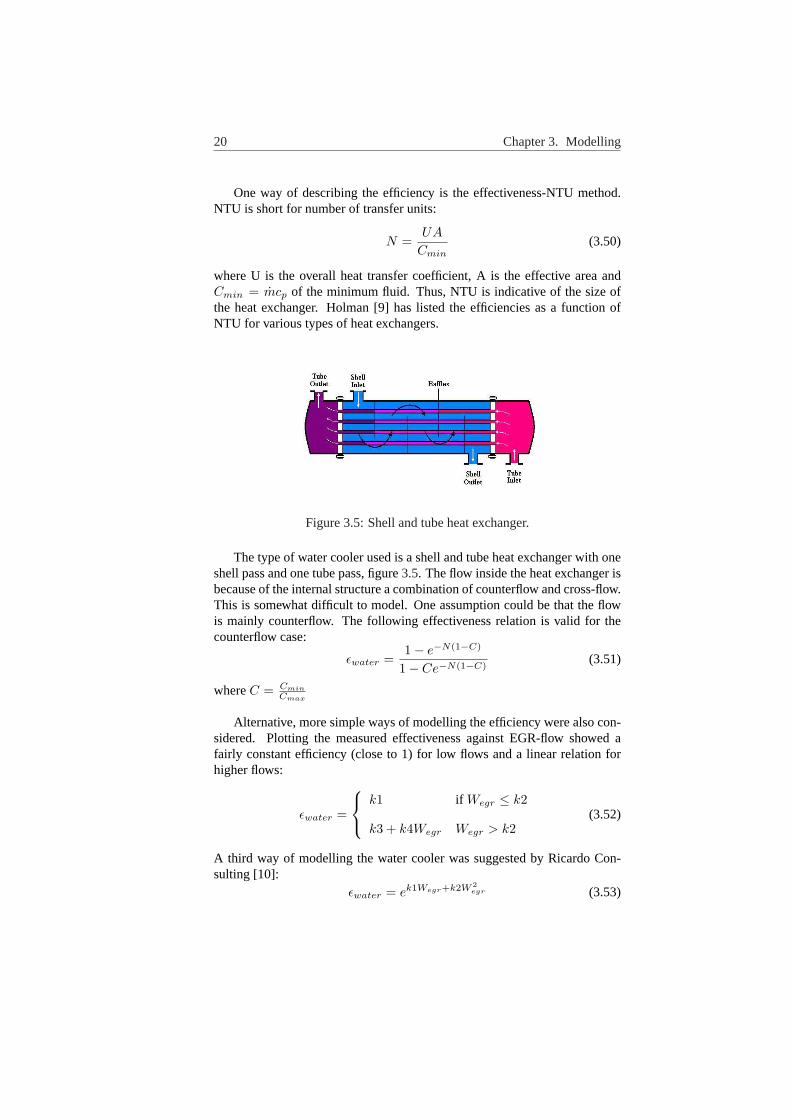
Figure 3.5:Shell and tube heat exchanger.
The type of water cooler used is a shell and tube heat exchanger with oneshell pass and one tube pass, figure3.5. The flow inside the heat exchanger isbecause of the internal structure a combination of counterflow and cross-flow.This is somewhat difficult to model. One assumption could be that the flowis mainly counterflow. The following effectiveness relation is valid for thecounterflow case:
εwater =1− e−N(1−C)
1− Ce−N(1−C)(3.51)
whereC = Cmin
Cmax
Alternative, more simple ways of modelling the efficiency were also con-sidered. Plotting the measured effectiveness against EGR-flow showed afairly constant efficiency (close to 1) for low flows and a linear relation forhigher flows:
εwater =
k1 if Wegr ≤ k2
k3 + k4Wegr Wegr > k2(3.52)
A third way of modelling the water cooler was suggested by Ricardo Con-sulting [10]:
εwater = ek1Wegr+k2W 2egr (3.53)
3.3. Extended Models 21
This relation was also derived on a purely empirical basis. The linear modelproved to offer the best performance out of the three models suggested andwas therefore chosen. The water cooler will suffer from fouling [11] whichwill lower the efficiency over time by up to 20%. This behavior has not beenmodelled.
The prototype air cooler on the test engine is a cross flow cooler, identicalto the charge air cooler, only smaller. The NTU-efficiency is given by:
εair = 1− ee−CN0.78−1
CN−0.22 (3.54)
As discussed in chapter2.2.3, the temperature after the air cooler is difficultto measure properly. Possibly because of this the NTU model was a poor fitto measurement data and therefore rejected. Superior results were achievedwith a constant efficiency:
εair = k1 (3.55)
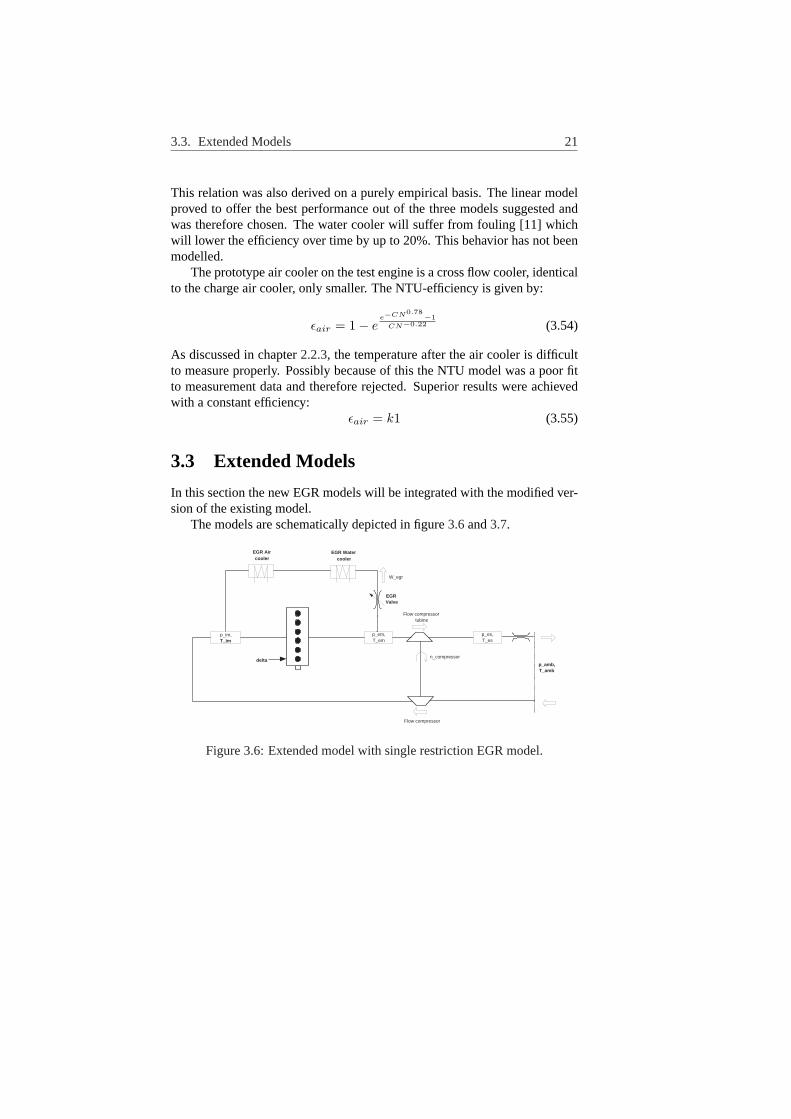
3.3 Extended Models
In this section the new EGR models will be integrated with the modified ver-sion of the existing model.
The models are schematically depicted in figure3.6and3.7.
p_em, T_em
p_im, T_im
n_compressor
Flow compressor tubine
Flow compressor
p_amb, T_amb
p_es, T_es
EGR Air cooler
delta
EGR Water cooler
EGR Valve
W_egr
Figure 3.6:Extended model with single restriction EGR model.
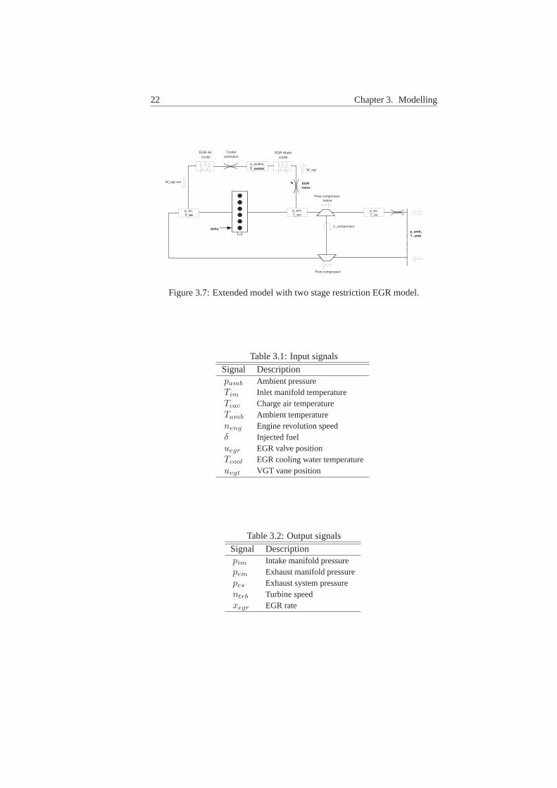
22 Chapter 3. Modelling
p_em, T_em
p_im, T_im
n_compressor
Flow compressor tubine
Flow compressor
p_amb, T_amb
p_es, T_es
EGR Air cooler
delta
EGR Water cooler
EGR Valve
p_avalve, T_awater
Cooler restriction
W_egr
W_egr,out
Figure 3.7:Extended model with two stage restriction EGR model.
Table 3.1:Input signals
Signal Descriptionpamb Ambient pressureTim Inlet manifold temperatureTcac Charge air temperatureTamb Ambient temperatureneng Engine revolution speedδ Injected fueluegr EGR valve positionTcool EGR cooling water temperatureuvgt VGT vane position
Table 3.2:Output signals
Signal Descriptionpim Intake manifold pressurepem Exhaust manifold pressurepes Exhaust system pressurentrb Turbine speedxegr EGR rate
Chapter 4
Tuning
All parameters were tuned using a set of 51 static points (separate from thedata set used in chapter5 for validation). Different operating conditions wereused, 1200, 1500 and 1900rpm at 25, 50, 75 and 100% load using manualadjustment of the VGT vane position and EGR valve position in order to coverthe whole range of EGR flows and valve positions. The entire engine modelhas not been tuned, only the new EGR model. For optimization, Lsoptim [4]was used.
4.1 Flow Model
The ”measured” effective flow area was calculated backwards from equation3.38using the measured value ofWegr.
4.1.1 Single restriction model
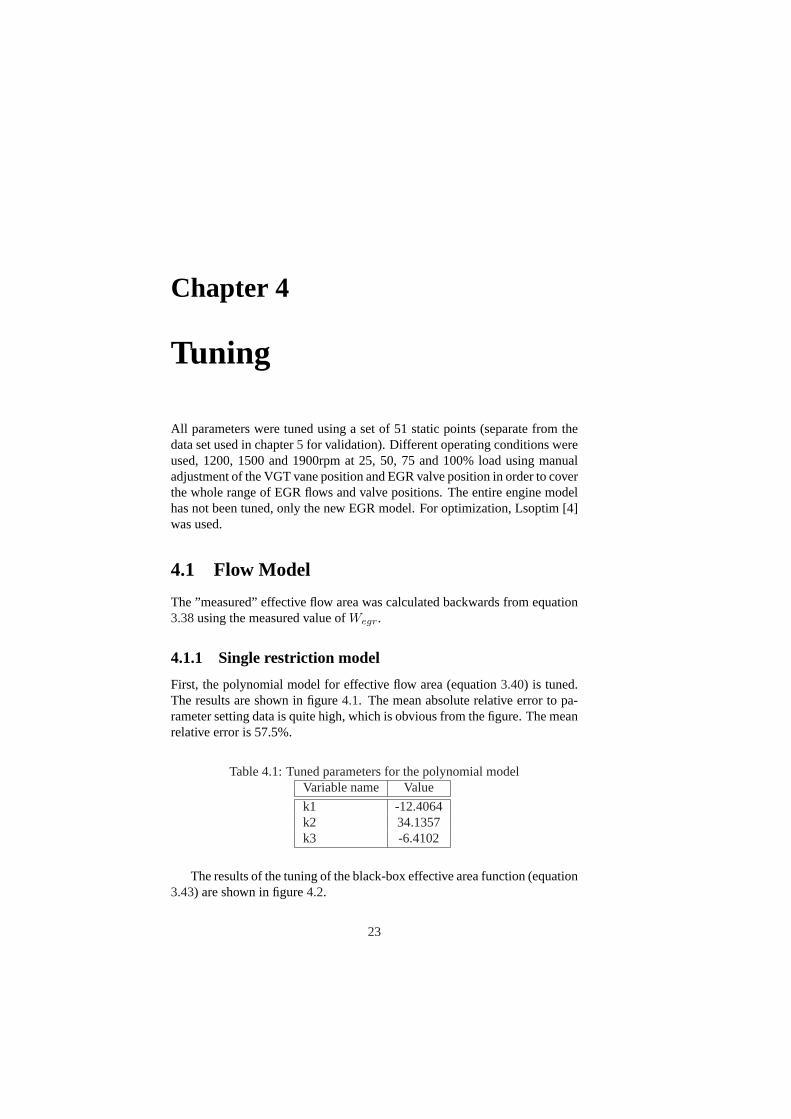
First, the polynomial model for effective flow area (equation3.40) is tuned.The results are shown in figure4.1. The mean absolute relative error to pa-rameter setting data is quite high, which is obvious from the figure. The meanrelative error is 57.5%.
Table 4.1:Tuned parameters for the polynomial modelVariable name Value
k1 -12.4064k2 34.1357k3 -6.4102
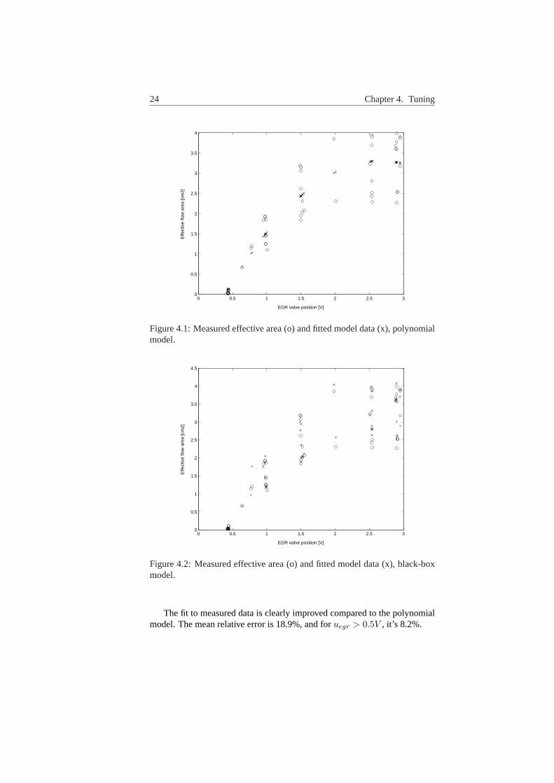
The results of the tuning of the black-box effective area function (equation3.43) are shown in figure4.2.
23
24 Chapter 4. Tuning
0 0.5 1 1.5 2 2.5 30
0.5
1
1.5
2
2.5
3
3.5
4
EGR valve position [V]
Effe
ctiv
e flo
w a
rea
[cm
2]
Figure 4.1:Measured effective area (o) and fitted model data (x), polynomialmodel.
0 0.5 1 1.5 2 2.5 30
0.5
1
1.5
2
2.5
3
3.5
4
4.5
EGR valve position [V]
Effe
ctiv
e flo
w a
rea
[cm
2]
Figure 4.2:Measured effective area (o) and fitted model data (x), black-boxmodel.
The fit to measured data is clearly improved compared to the polynomialmodel. The mean relative error is 18.9%, and foruegr > 0.5V , it’s 8.2%.
4.1. Flow Model 25
Table 4.2:Tuned parameters for the black-box modelVariable name Value
a1 -3.0038a2 3.5947a3 0.3082a4 -1.9045a5 4.9567a6 -1.1311
4.1.2 Two stage restriction model
In this section a combination of manual tuning and Lsoptim has been used forpractical reasons. The basis for this optimization work has been to optimizethe EGR flow to measured data for the complete EGR system, using measuredpem andpim (static pressures) for inputs and ignoring the unreliablepavalve
andpawater. During the optimization process, only static data was used, andthereforeVegr cannot be estimated and alsoWegr = Wegr,out.
The constantsk1 andk2 in the cooler restriction were optimized to give apavalve which will suit equation3.38optimally.
Table 4.3:Tuned parameters for the cooler restrictionVariable name Value
k1 -0.0002k2 0.07
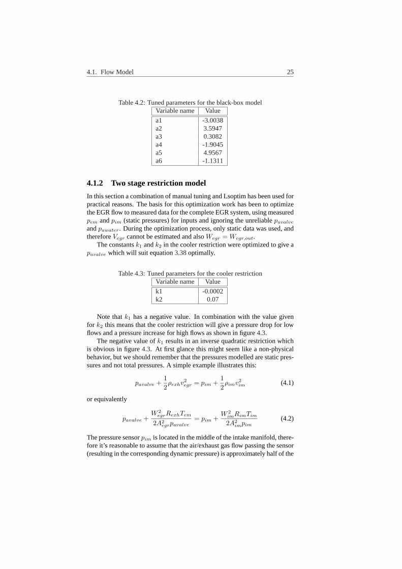
Note thatk1 has a negative value. In combination with the value givenfor k2 this means that the cooler restriction will give a pressure drop for lowflows and a pressure increase for high flows as shown in figure4.3.
The negative value ofk1 results in an inverse quadratic restriction whichis obvious in figure4.3. At first glance this might seem like a non-physicalbehavior, but we should remember that the pressures modelled are static pres-sures and not total pressures. A simple example illustrates this:
pavalve +12ρexhv2
egr = pim +12ρimv2
im (4.1)
or equivalently
pavalve +W 2
egrRexhTem
2A2egrpavalve
= pim +W 2
imRimTim
2A2impim
(4.2)
The pressure sensorpim is located in the middle of the intake manifold, there-fore it’s reasonable to assume that the air/exhaust gas flow passing the sensor(resulting in the corresponding dynamic pressure) is approximately half of the
26 Chapter 4. Tuning
0 0.02 0.04 0.06 0.08 0.1 0.12 0.14−0.15
−0.1
−0.05
0
0.05
0.1
EGR flow [kg/s]
Pre
ssur
e di
ffere
nce
[bar
]
Figure 4.3:Pressure difference vs. EGR flow.
total intake manifold flow. In order to get a qualitative feeling for the impactof the dynamic pressures,pim andpavalve are both assumed to be in the 2bar range, an exhaust temperature of 700K, an intake temperature of 300K,an EGR flow of 0.14kg/s (the highest practically occurring flow), a 28% EGRrate resulting in an air flow of 0.50kg/s and finally the areas were assumed tobe7cm2 and24cm2 respectively. This results in:
pavalve − pim = −0.16bar (4.3)
which confirms that an increase in the static pressure over the EGR coolers ispossible because of the decrease in dynamic pressure.
Using the calculated pressurepavalve from the cooler restriction modelas an input to equation3.38 the dispersion in effective flow area is reducedcompared to the single restriction model. The simple non-compensated poly-nomial function for effective flow area is now a much better fit, see figure4.4.
The mean absolute relative error while fitting the model to parameter set-ting data is 22.1%, and foruegr > 0.5V , it’s only 5.1%.
4.2 Temperature model
4.2.1 Water cooler
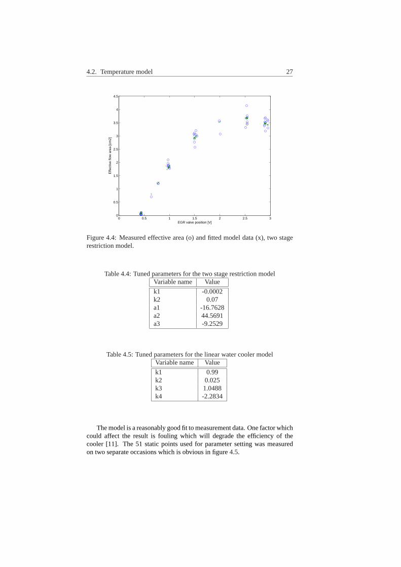
The linear model suggested in chapter3.2.2was tuned using Lsoptim. Theresults are shown in table4.5and the fitting of the model to parameter settingdata in figure4.5.
4.2. Temperature model 27
0 0.5 1 1.5 2 2.5 30
0.5
1
1.5
2
2.5
3
3.5
4
4.5
EGR valve position [V]
Effe
ctiv
e flo
w a
rea
[cm
2]
Figure 4.4:Measured effective area (o) and fitted model data (x), two stagerestriction model.
Table 4.4:Tuned parameters for the two stage restriction modelVariable name Value
k1 -0.0002k2 0.07a1 -16.7628a2 44.5691a3 -9.2529
Table 4.5:Tuned parameters for the linear water cooler modelVariable name Value
k1 0.99k2 0.025k3 1.0488k4 -2.2834
The model is a reasonably good fit to measurement data. One factor whichcould affect the result is fouling which will degrade the efficiency of thecooler [11]. The 51 static points used for parameter setting was measuredon two separate occasions which is obvious in figure4.5.
28 Chapter 4. Tuning
0 0.02 0.04 0.06 0.08 0.1 0.12 0.140.7
0.75
0.8
0.85
0.9
0.95
1
EGR flow [kg/s]
Effi
cien
cy
Figure 4.5:Measured cooler efficiency (o) and fitted model data (x).
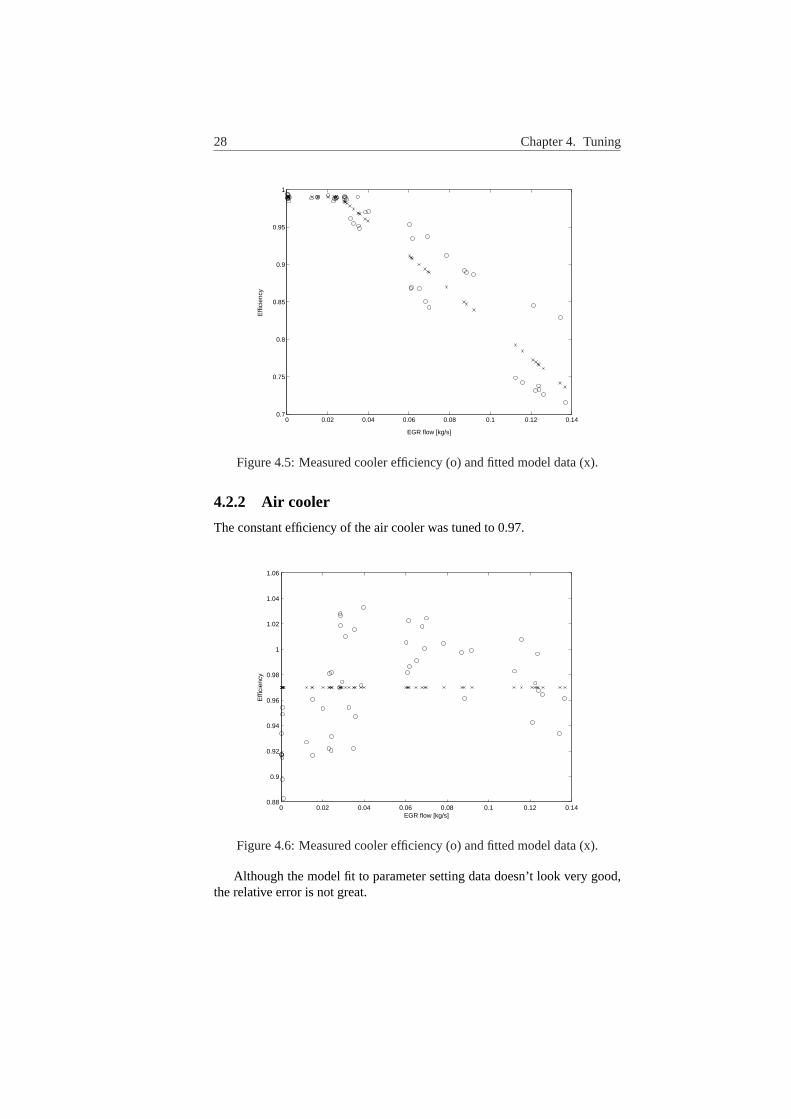
4.2.2 Air cooler
The constant efficiency of the air cooler was tuned to 0.97.
0 0.02 0.04 0.06 0.08 0.1 0.12 0.140.88
0.9
0.92
0.94
0.96
0.98
1
1.02
1.04
1.06
EGR flow [kg/s]
Effi
cien
cy
Figure 4.6:Measured cooler efficiency (o) and fitted model data (x).
Although the model fit to parameter setting data doesn’t look very good,the relative error is not great.
Chapter 5
Validation
In this chapter, the models are validated using a set of 28 static points col-lected in the engine test bed. Error is measured by the measures mean errorand maximal error. Also, the error distribution is analyzed using histogramplots.
mean relative error =1n
n∑
i=1
|x(ti)− x(ti)||x(ti)| (5.1)
maximum relative error = max1≤i≤n
|x(ti)− x(ti)||x(ti)| , (5.2)
wherex(ti) is the measured quantity,x(ti) is the simulated quantity andn isthe number of samples.
5.1 Flow Model
The three different EGR valve model configurations presented are validatedin this section.
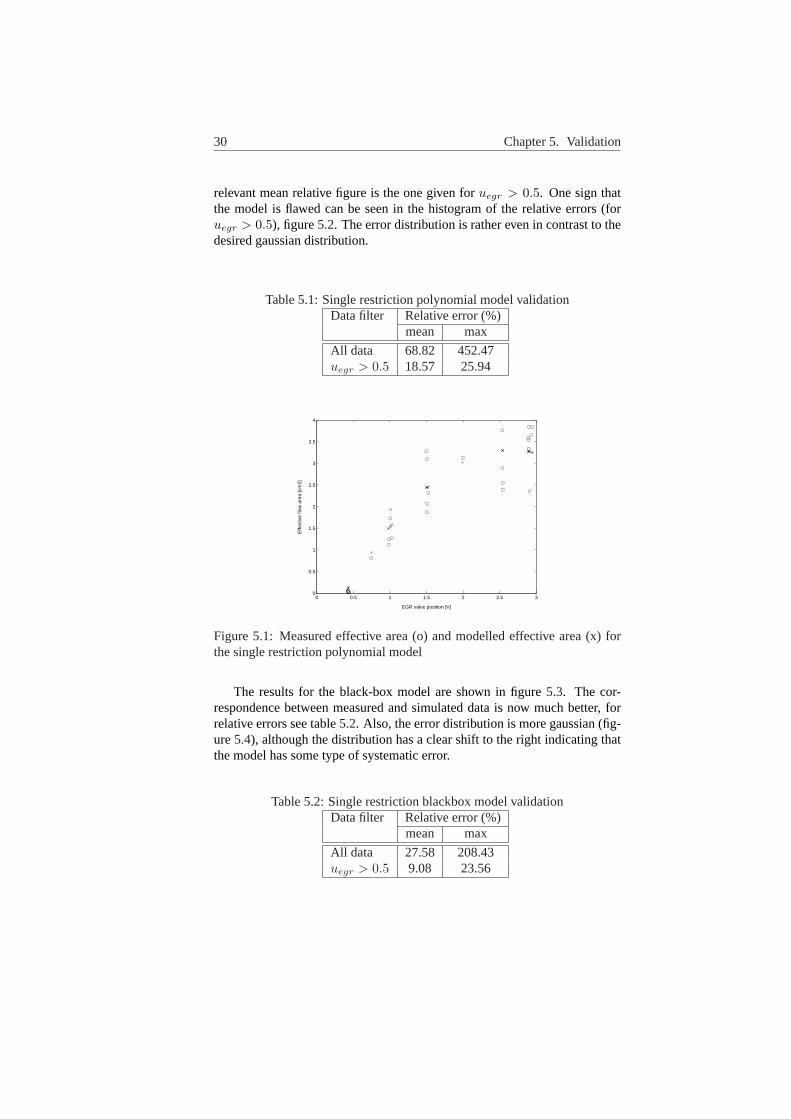
5.1.1 Single restriction model
The measured and modelled effective areas for the simple polynomial modelare shown in figure5.1 . The fit is not very good, for corresponding meanand max errors, see table5.1. Note that the relative errors are much lower ifthe data for a almost fully closed valve (uegr ≤ 0.5) is excluded. The rela-tive error for these almost closed valve positions is not of great significancebecause of the extremely low flows. A relative error of 100% in these caseswould imply an EGR rate of for example 0.2% instead of the actual 0.1%.This will have a very small impact on the model as a whole. Therefore, the
29
30 Chapter 5. Validation
relevant mean relative figure is the one given foruegr > 0.5. One sign thatthe model is flawed can be seen in the histogram of the relative errors (foruegr > 0.5), figure5.2. The error distribution is rather even in contrast to thedesired gaussian distribution.
Table 5.1:Single restriction polynomial model validationData filter Relative error (%)
mean max
All data 68.82 452.47uegr > 0.5 18.57 25.94
0 0.5 1 1.5 2 2.5 30
0.5
1
1.5
2
2.5
3
3.5
4
EGR valve position [V]
Effe
ctiv
e flo
w a
rea
[cm
2]
Figure 5.1:Measured effective area (o) and modelled effective area (x) forthe single restriction polynomial model
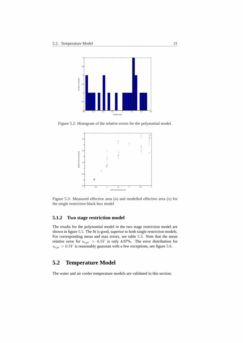
The results for the black-box model are shown in figure5.3. The cor-respondence between measured and simulated data is now much better, forrelative errors see table5.2. Also, the error distribution is more gaussian (fig-ure5.4), although the distribution has a clear shift to the right indicating thatthe model has some type of systematic error.
Table 5.2:Single restriction blackbox model validationData filter Relative error (%)
mean max
All data 27.58 208.43uegr > 0.5 9.08 23.56
5.2. Temperature Model 31
−0.4 −0.3 −0.2 −0.1 0 0.1 0.2 0.30
0.5
1
1.5
2
2.5
3
Relative fault
Num
ber
of s
ampl
es
Figure 5.2:Histogram of the relative errors for the polynomial model.
0 0.5 1 1.5 2 2.5 3−0.5
0
0.5
1
1.5
2
2.5
3
3.5
4
EGR valve position [V]
Effe
ctiv
e flo
w a
rea
[cm
2]
Figure 5.3:Measured effective area (o) and modelled effective area (x) forthe single restriction black-box model
5.1.2 Two stage restriction model
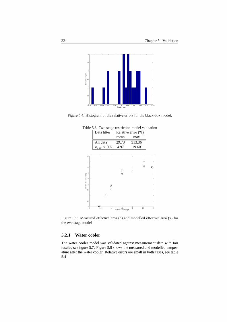
The results for the polynomial model in the two stage restriction model areshown in figure5.5. The fit is good, superior to both single restriction models.For corresponding mean and max errors, see table5.3. Note that the meanrelative error foruegr > 0.5V is only 4.97%. The error distribution foruegr > 0.5V is reasonably gaussian with a few exceptions, see figure5.6.
5.2 Temperature Model
The water and air cooler temperature models are validated in this section.
32 Chapter 5. Validation
−0.25 −0.2 −0.15 −0.1 −0.05 0 0.05 0.1 0.15 0.2 0.250
0.5
1
1.5
2
2.5
3
Relative fault
Num
ber
of s
ampl
es
Figure 5.4:Histogram of the relative errors for the black-box model.
Table 5.3:Two stage restriction model validationData filter Relative error (%)
mean max
All data 29.73 313.36uegr > 0.5 4.97 19.60
0 0.5 1 1.5 2 2.5 30
0.5
1
1.5
2
2.5
3
3.5
4
4.5
EGR valve position [V]
Effe
ctiv
e flo
w a
rea
[cm
2]
Figure 5.5:Measured effective area (o) and modelled effective area (x) forthe two stage model
5.2.1 Water cooler
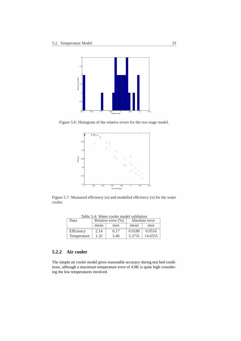
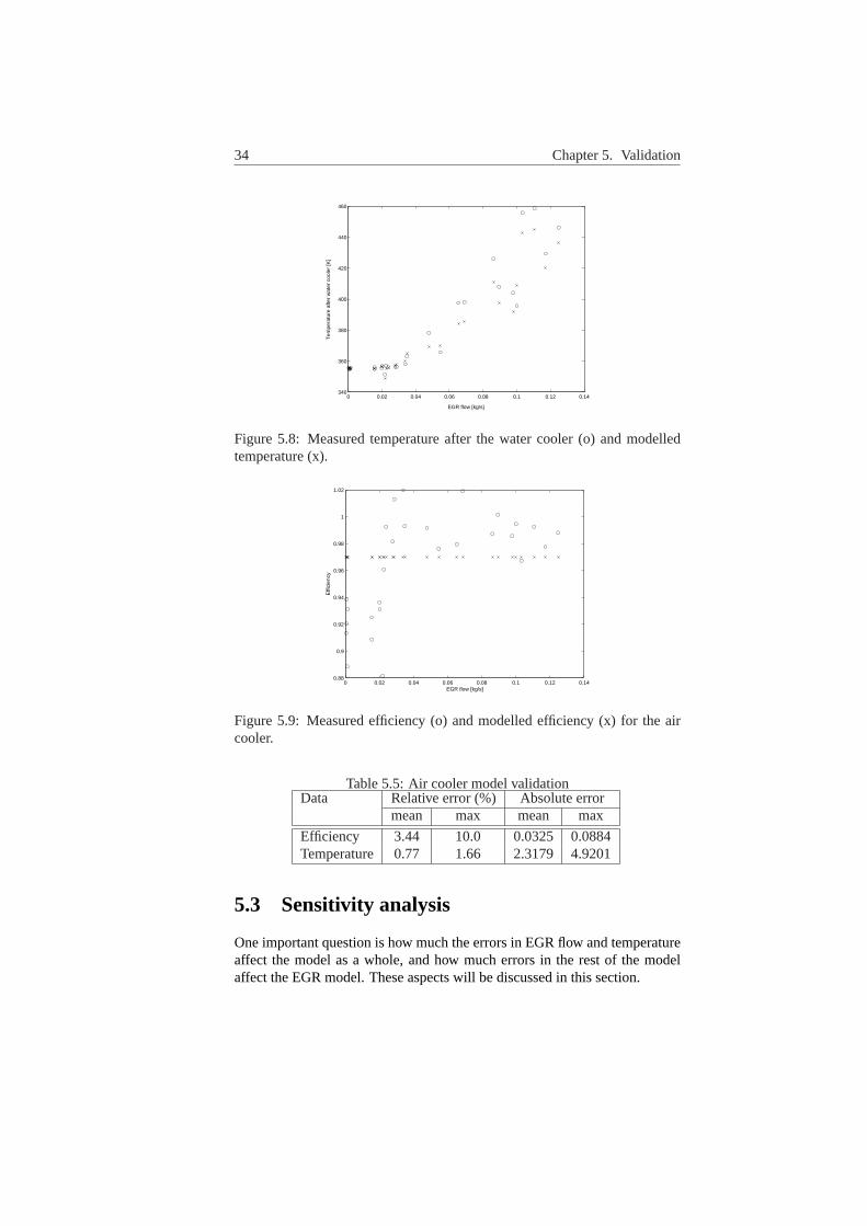
The water cooler model was validated against measurement data with fairresults, see figure5.7. Figure5.8shows the measured and modelled temper-ature after the water cooler. Relative errors are small in both cases, see table5.4
5.2. Temperature Model 33
−0.2 −0.15 −0.1 −0.05 0 0.05 0.1 0.150
0.5
1
1.5
2
2.5
3
Relative fault
Num
ber
of s
ampl
es
Figure 5.6:Histogram of the relative errors for the two stage model.
0 0.02 0.04 0.06 0.08 0.1 0.12 0.140.7
0.75
0.8
0.85
0.9
0.95
1
EGR flow [kg/s]
Effi
cien
cy
Figure 5.7:Measured efficiency (o) and modelled efficiency (x) for the watercooler.
Table 5.4:Water cooler model validationData Relative error (%) Absolute error
mean max mean max
Efficiency 2.14 6.17 0.0180 0.0516Temperature 1.32 3.46 5.3731 14.6555
5.2.2 Air cooler
The simple air cooler model gives reasonable accuracy during test bed condi-tions, although a maximum temperature error of 4.9K is quite high consider-ing the low temperatures involved.
34 Chapter 5. Validation
0 0.02 0.04 0.06 0.08 0.1 0.12 0.14340
360
380
400
420
440
460
EGR flow [kg/s]
Tem
pera
ture
afte
r w
ater
coo
ler
[K]
Figure 5.8: Measured temperature after the water cooler (o) and modelledtemperature (x).
0 0.02 0.04 0.06 0.08 0.1 0.12 0.140.88
0.9
0.92
0.94
0.96
0.98
1
1.02
EGR flow [kg/s]
Effi
cien
cy
Figure 5.9:Measured efficiency (o) and modelled efficiency (x) for the aircooler.
Table 5.5:Air cooler model validationData Relative error (%) Absolute error
mean max mean max
Efficiency 3.44 10.0 0.0325 0.0884Temperature 0.77 1.66 2.3179 4.9201
5.3 Sensitivity analysis
One important question is how much the errors in EGR flow and temperatureaffect the model as a whole, and how much errors in the rest of the modelaffect the EGR model. These aspects will be discussed in this section.
5.3. Sensitivity analysis 35
0 0.02 0.04 0.06 0.08 0.1 0.12 0.14294
296
298
300
302
304
306
EGR flow [kg/s]
Tem
pera
ture
afte
r ai
r co
oler
[K]
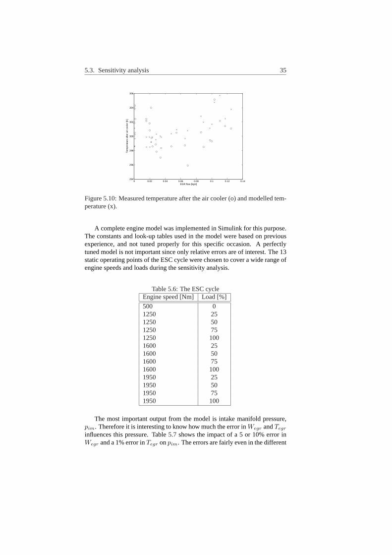
Figure 5.10:Measured temperature after the air cooler (o) and modelled tem-perature (x).
A complete engine model was implemented in Simulink for this purpose.The constants and look-up tables used in the model were based on previousexperience, and not tuned properly for this specific occasion. A perfectlytuned model is not important since only relative errors are of interest. The 13static operating points of the ESC cycle were chosen to cover a wide range ofengine speeds and loads during the sensitivity analysis.
Table 5.6:The ESC cycleEngine speed [Nm] Load [%]
500 01250 251250 501250 751250 1001600 251600 501600 751600 1001950 251950 501950 751950 100
The most important output from the model is intake manifold pressure,pim. Therefore it is interesting to know how much the error inWegr andTegr
influences this pressure. Table5.7 shows the impact of a 5 or 10% error inWegr and a 1% error inTegr onpim. The errors are fairly even in the different
36 Chapter 5. Validation
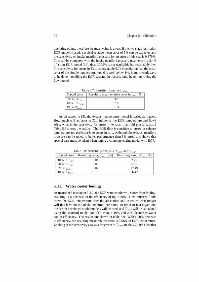
operating points, therefore the mean value is given. If the two stage restrictionEGR model is used, a typical relative mean error of 5% can be expected andthe sensitivity on intake manifold pressure for an error of this size is 0.379%.This can be compared with the intake manifold pressure mean error of 3.4%of a non-EGR model [14], thus 0.379% is not negligible but reasonably low.The sensitivity for errors inTaair is low (table5.7), considering that the meanerror of the simple temperature model is well below 1%. If more work wereto be done modelling the EGR system, the focus should be on improving theflow model.
Table 5.7:Sensitivity analysis,pim
Forced error Resulting mean relative error inpim [%]
5% inWegr 0.37910% inWegr 0.7591% inTaair 0.131
As discussed in [5], the exhaust temperature model is seriously flawed.How much will an error inTem influence the EGR temperature and flow?Also, what is the sensitivity for errors in exhaust manifold pressure,pem?Table5.8 shows the results. The EGR flow is sensitive to errors in exhausttemperature and particularly to errors inpem. Although the exhaust manifoldpressure can be tuned to better performance than 5% error, this shows thatspecial care must be taken when tuning a complete engine model with EGR.
Table 5.8:Sensitivity analysis,Taair andWegr
Forced error Resulting error,Taair [%] Resulting error,Wegr [%]
10% inTem 0.04 2.7920% inTem 0.08 5.685% inpem 0.07 17.4910% inpem 0.13 26.47
5.3.1 Water cooler fouling
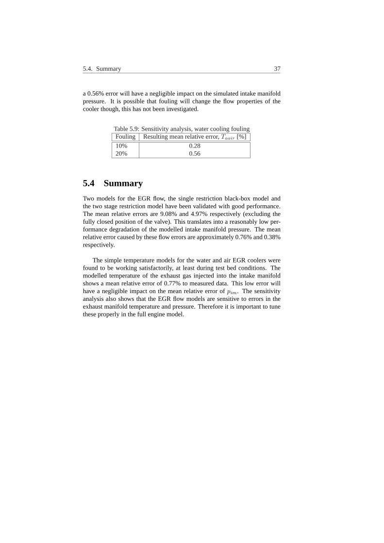
As mentioned in chapter3.2.2, the EGR water cooler will suffer from fouling,resulting in a decrease in the efficiency of up to 20%. How much will thisaffect the EGR temperature after the air cooler, and in return what impactwill this have on the intake manifold pressure? In order to investigate thisthe earlier developed cooler models will be used, andTaair will be calculatedusing the standard model and also using a 10% and 20% decreased watercooler efficiency. The results are shown in table5.9. With a 20% decreasein efficiency, the resulting mean relative error is 0.56% in EGR temperature.Looking at the sensitivity analysis for errors inTaair (table5.7), it’s clear that
5.4. Summary 37
a 0.56% error will have a negligible impact on the simulated intake manifoldpressure. It is possible that fouling will change the flow properties of thecooler though, this has not been investigated.
Table 5.9:Sensitivity analysis, water cooling foulingFouling Resulting mean relative error,Taair [%]
10% 0.2820% 0.56
5.4 Summary
Two models for the EGR flow, the single restriction black-box model andthe two stage restriction model have been validated with good performance.The mean relative errors are 9.08% and 4.97% respectively (excluding thefully closed position of the valve). This translates into a reasonably low per-formance degradation of the modelled intake manifold pressure. The meanrelative error caused by these flow errors are approximately 0.76% and 0.38%respectively.
The simple temperature models for the water and air EGR coolers werefound to be working satisfactorily, at least during test bed conditions. Themodelled temperature of the exhaust gas injected into the intake manifoldshows a mean relative error of 0.77% to measured data. This low error willhave a negligible impact on the mean relative error ofpim. The sensitivityanalysis also shows that the EGR flow models are sensitive to errors in theexhaust manifold temperature and pressure. Therefore it is important to tunethese properly in the full engine model.
Chapter 6
Conclusions and FutureWork
6.1 Conclusions
Two models for the EGR flow have been developed and successfully tested.The single restriction black-box model features a low complexity and a meanrelative error of 9.08% during static conditions. The two stage restrictionmodel is of higher complexity and has a mean relative error of 4.97%, whichis low enough considering that the sensitivity analysis showed that a 5% EGRflow error gives an error in the modelled intake manifold pressure of only0.38%. Both models give big improvements over the previously used EGRmodels. The intake manifold model has been modified to take temperaturefluctuations into account. The temperature model suggested has also beentested with good performance. The 0.77% mean relative error in EGR tem-perature has a negligible impact on the model as a whole. Fouling of thewater EGR cooler of up to 20% reduced efficiency will also have a very smallimpact on the complete model.
6.2 Future Work
During the work with this thesis a couple of interesting areas for further in-vestigations have come up. In this section some of them are presented.
The most important future work is to validate the model using dynamicmeasurement data. In order to do this the entire model must be tuned, there iscurrently no way to measure the EGR flow dynamically making a validationof the EGR system separate from the rest of the model difficult. A data col-lecting system with a higher sampling rate than the test bed computer alongwith faster temperature sensors are also essential.
38
6.2. Future Work 39
It would be interesting to validate the EGR cooler temperature models ina truck or in a test bed with climate control to investigate their behavior atambient temperatures different from 298K.
Investigating pressure pulsations and their influence on exhaust and intakemanifold pressure is of great interest if further improvements are to be madeon the EGR flow model. Is it possible to compensate the mean value modelin order to model these pulsations? A measurement system with a high sam-pling rate along with high speed pressure sensors would be useful. Measuringdynamic pressure would be useful in order to reinforce the motivation for theinverse quadratic cooler restriction.
In order to make the model more physical and also simplifying the tuning,the turbine and compressor look-up tables could be replaced with physicallybased equations. Some work has been done in this field [16], although inte-gration with the new EGR models and further validation under dynamic con-ditions is needed. One possible disadvantage with physically based equationsis that limitations could be revealed in the other models.
References
[1] J. Biteus. MVEM of DC12 scania engine. Technical report, Departmentof Electrical Engineering, Linkoping University, May 2002.
[2] I. Ekroth and E. Granryd.Till ampad termodynamik. Institutionen forEnergiteknik, KTH, 1999.
[3] D. Elfvik. Modelling of a diesel engine with vgt for control design sim-ulations. Master’s thesis IR-RT-EX-0216, Department of Signals, Sen-sors and Systems, Royal Institute of Technology, Stockholm, Sweden,July 2002.
[4] L. Eriksson. A Minimal Manual to lsoptim. Department of ElectricalEngineering, Linkopings Universitet.
[5] O. Flardh and M. Gustafson. Mean value modelling of a diesel enginewith turbo compound. Master’s thesis LiTH-ISY-EX-3443, Departmentof Electrical Engineering, Linkoping University, Linkoping, Sweden,December 2003.
[6] M. Fons, M. Muller, A. Chevalier, C. Vigild, E. Hendricks, and S. Soren-son. Mean value modelling of an si engine with egr. InSI Engine Mod-eling, Detroit, Michigan, USA, 1999. SAE.
[7] L. Guzzela and A. Amstutz. Control of diesel engines.IEEE ControlSystems, AC-37(7):53–71, October 1998.
[8] J. B. Heywood.Internal Combustion Engine Fundamentals. McGrae-Hill, 1988.
[9] J. P. Holman.Heat Transfer. McGrae-Hill, 9th edition, 2002.
[10] G. N. Kennedy. Scania diesel egr control project description of dynamicengine simulation model version 1.1. Internal Scania document, 1996.
[11] J. Mardberg. Prov av egrkylarnedsmutsning. Internal Scania document,2001.
40
References 41
[12] M. Nyberg, T. Stutte, and V. Wilhelmi. Model based diagnosis of the airpath of an automotive diesel engine. InIFAC Workshop: Advances inAutomotive Control, Karlsruhe, Germany, 2001. IFAC Workshop: Ad-vances in Automotive Control.
[13] S. Oberg. Identification and improvements of an automotive diesel en-gine model purposed for model based diagnosis. Master’s thesis LiTH-ISY-EX-3161, Department of Electrical Engineering, Linkoping Uni-versity, Linkoping, Sweden, December 2001.
[14] J. Ritzen. Modelling and fixed step simulation of a turbo charged dieselengine. Master’s thesis LiTH-ISY-EX-3442, Department of ElectricalEngineering, Linkoping University, Linkoping, Sweden, June 2003.
[15] P. Skogtjarn. Modelling of the exhaust gas temperature for dieselengines. Master’s thesis LiTH-ISY-EX-3378, Department of Electri-cal Engineering, Linkoping University, Linkoping, Sweden, December2002.
[16] J. Wahlstrom. Modelling of a diesel engine with vgt and egr. Techni-cal report, Department of Electrical Engineering, Linkoping University,2004.
Notation
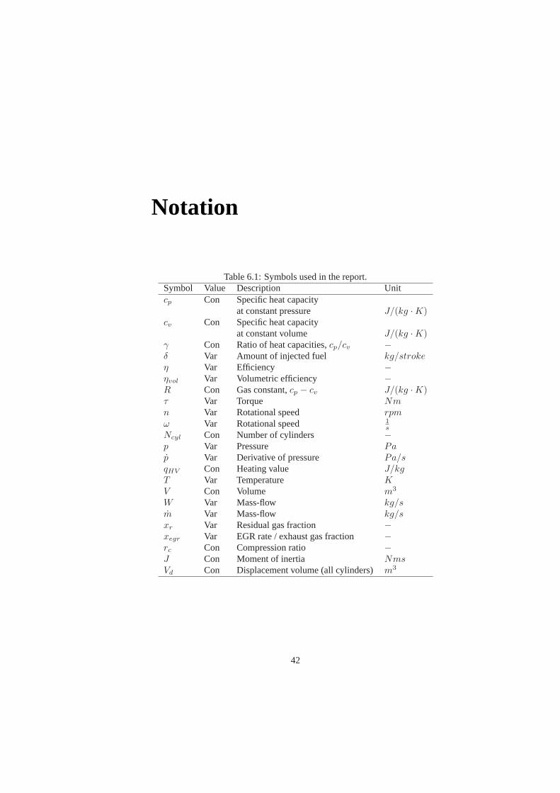
Table 6.1:Symbols used in the report.Symbol Value Description Unitcp Con Specific heat capacity
at constant pressure J/(kg ·K)cv Con Specific heat capacity
at constant volume J/(kg ·K)γ Con Ratio of heat capacities,cp/cv −δ Var Amount of injected fuel kg/strokeη Var Efficiency −ηvol Var Volumetric efficiency −R Con Gas constant,cp − cv J/(kg ·K)τ Var Torque Nmn Var Rotational speed rpmω Var Rotational speed 1
sNcyl Con Number of cylinders −p Var Pressure Pap Var Derivative of pressure Pa/sqHV Con Heating value J/kgT Var Temperature KV Con Volume m3
W Var Mass-flow kg/sm Var Mass-flow kg/sxr Var Residual gas fraction −xegr Var EGR rate / exhaust gas fraction −rc Con Compression ratio −J Con Moment of inertia NmsVd Con Displacement volume (all cylinders)m3
42
Notation 43
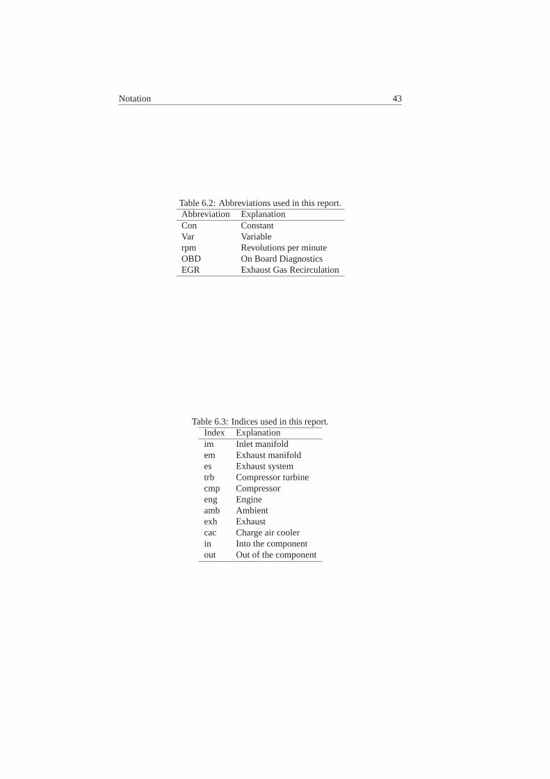
Table 6.2:Abbreviations used in this report.Abbreviation ExplanationCon ConstantVar Variablerpm Revolutions per minuteOBD On Board DiagnosticsEGR Exhaust Gas Recirculation
Table 6.3:Indices used in this report.Index Explanationim Inlet manifoldem Exhaust manifoldes Exhaust systemtrb Compressor turbinecmp Compressoreng Engineamb Ambientexh Exhaustcac Charge air coolerin Into the componentout Out of the component