mean-variance portfolio optimization: do historical...

Mean-variance portfolio optimization: do historical correlations

help or hinder risk control in a crisis?

Tony PlatePlate Consulting, LLC

Santa Fe, NM

[email protected]

(*some of this research performed atBlack Mesa Capital)

Expanded version of presentation with additional slides and explanations, 2010/05/29.

1

mailto:[email protected]

Mean-Variance optimization

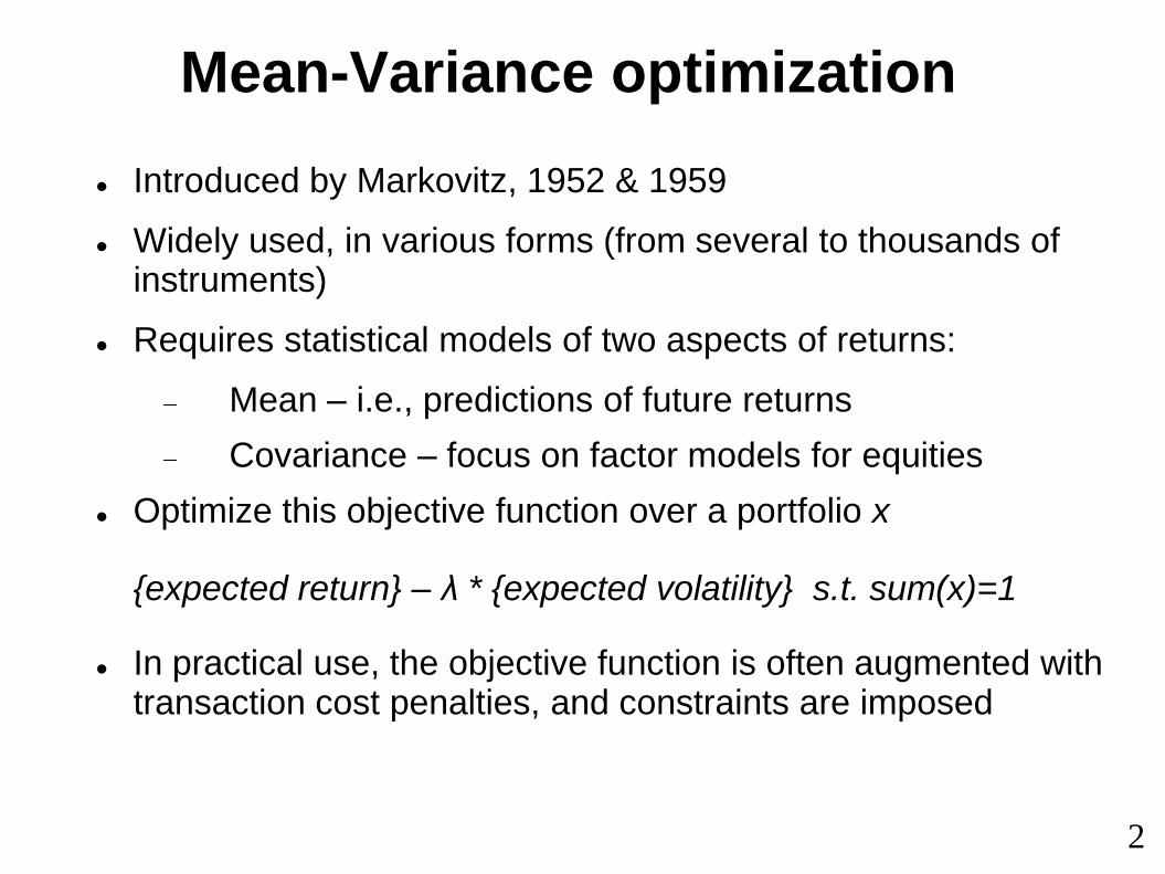
Introduced by Markovitz, 1952 & 1959

Widely used, in various forms (from several to thousands of instruments)

Requires statistical models of two aspects of returns:

Mean – i.e., predictions of future returns

Covariance – focus on factor models for equities

Optimize this objective function over a portfolio x

{expected return} – λ * {expected volatility} s.t. sum(x)=1

In practical use, the objective function is often augmented with transaction cost penalties, and constraints are imposed

2

Quotes

From “The Emperor has no Clothes: Limits to Risk Modeling” (Jon Danielsson, 2001)

• “The fundamental assumption in most statistical risk modeling is that the basic statistical properties of financial data during stable periods remain (almost) the same as during a crisis. This of course is not correct.”

• [Unlike forecasting the weather] “forecasting risk does change the nature of risk”

• “Correlations typically underestimate the joint risk of two or more assets”

3

Note: Danielsson’s paper mostly focused on the use VaR, but his comments were also directed at the use of correlations

Quotes

From “Nickels and Dimes: Izzy Englander's Growth Strategy for Millennium” (Stephen Taub, Institutional Investor Magazine, 20 May 2009)

“Millennium Management founder Izzy Englander delivers consistently good returns by making low-risk bets that other hedge fund managers often ignore..."

“Millennium does not put much emphasis on the correlation between different investment strategies when deciding how to allocate capital. “That [approach] would have broken down last year,” points out Larkin, 34, who has day-to-day oversight responsibility for Millennium’s equities operation. “In a stress environment correlation goes to 1,” he says.

4

Quotes

From “Time-varying Stock Market Correlations and Correlation Breakdown” (David Michael Rey, 2000)

[Abstract]

“… recent experience has highlighted the fact that international equity correlations can rise quickly and dramatically. These so-called correlation breakdowns call into question the usefulness of diversifying and hedging operations based on correlations estimated from historical data, since they may be inaccurate precisely when they are most desired, namely in periods of high volatility or worse, extreme negative price movements…”

5

Literature Background

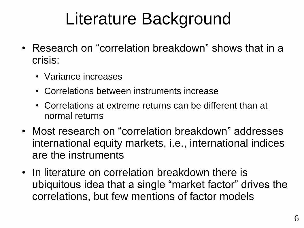
• Research on “correlation breakdown” shows that in a crisis:

• Variance increases

• Correlations between instruments increase

• Correlations at extreme returns can be different than at normal returns

• Most research on “correlation breakdown” addresses international equity markets, i.e., international indices are the instruments

• In literature on correlation breakdown there is ubiquitous idea that a single “market factor” drives the correlations, but few mentions of factor models

6

Question for this talk

• Can a factor model capture some of the dynamic statistics of variance and correlations of US equities during a crisis?

• Is mean-variance optimization (MVO) potentially useful or harmful during a crisis?

• Does the use of correlations in MVO hurt, help, or not matter during a crisis?

• Keep everything very simple and focus solely on risk control

• Recognize that the statistical assumptions of MVO are not satisfied by markets, esp during a crisis

7

Minimum Variance Portfolios

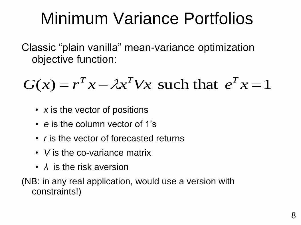
Classic “plain vanilla” mean-variance optimization objective function:

• x is the vector of positions

• e is the column vector of 1’s

• r is the vector of forecasted returns

• V is the co-variance matrix

• λ is the risk aversion

(NB: in any real application, would use a version with constraints!)

1 such that )( xeVxxxrxG TTT

8

Closed-form solution

Solution:

For very large λ (infinite), we get the minimum risk portfolio:

R code:

> iV <- solve(V)

> h_c <- rowSums(iV) / sum(iV)

More efficient:

> iV1 <- solve(V, 1)

> h_c <- iv1 / sum(iV1) (*beware rank-deficient V !)

eVe

eVrVerVh

T

T

1

111

)2

1(2

)(

eVe

eVh

Tc 1

1

9

Note: This very simple formulation of mean-variance optimization has an easily computable closed-form solutionFor maximum risk aversion, the dependence on r drops out and the minimum risk portfolio is a function of just the covariance matrix

Focus on minimum-variance portfolio

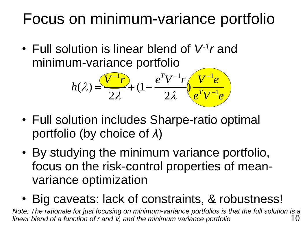
• Full solution is linear blend of V-1r and minimum-variance portfolio

• Full solution includes Sharpe-ratio optimal portfolio (by choice of λ)

• By studying the minimum variance portfolio, focus on the risk-control properties of mean-variance optimization

• Big caveats: lack of constraints, & robustness!

eVe

eVrVerVh

T

T

1

111

)2

1(2

)(

10Note: The rationale for just focusing on minimum-variance portfolios is that the full solution is a linear blend of a function of r and V, and the minimum variance portfolio

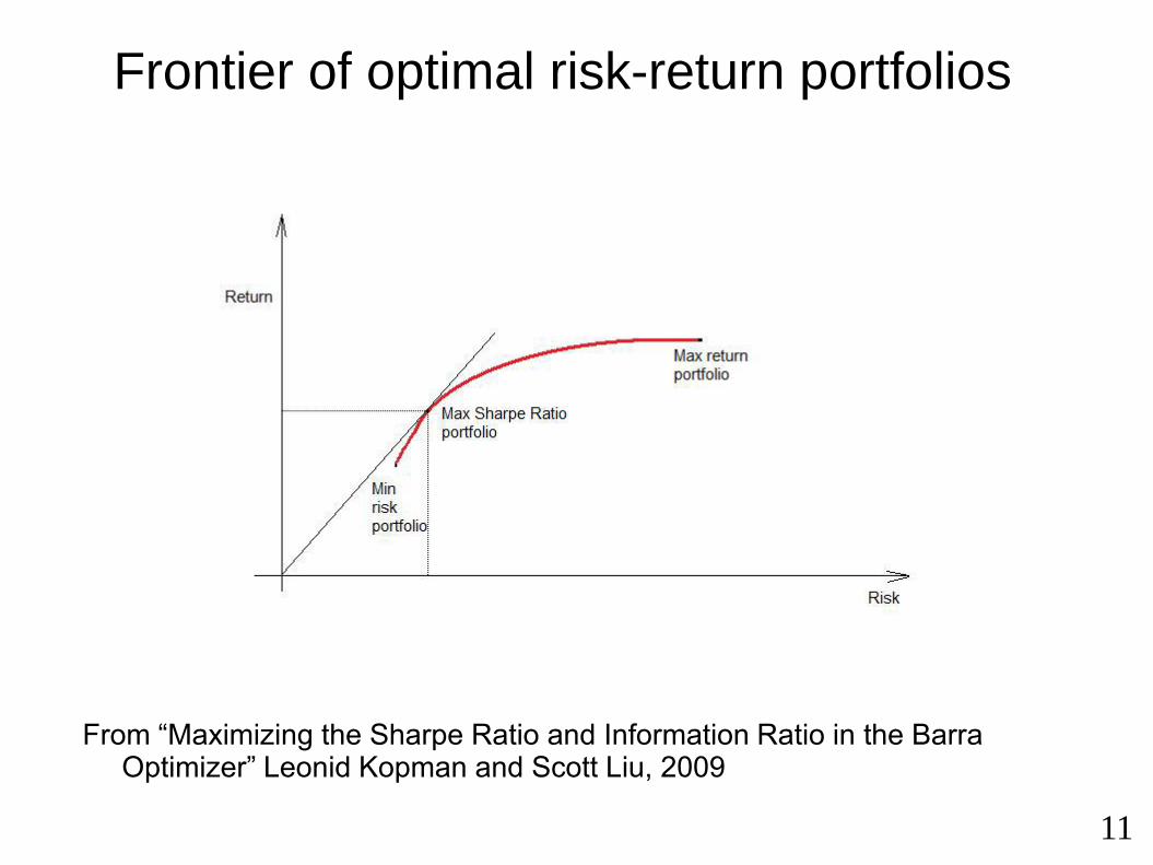
Frontier of optimal risk-return portfolios

From “Maximizing the Sharpe Ratio and Information Ratio in the Barra Optimizer” Leonid Kopman and Scott Liu, 2009

11

Assessment of risk models

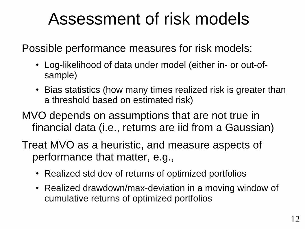
Possible performance measures for risk models:

• Log-likelihood of data under model (either in- or out-of-sample)

• Bias statistics (how many times realized risk is greater than a threshold based on estimated risk)

MVO depends on assumptions that are not true in financial data (i.e., returns are iid from a Gaussian)

Treat MVO as a heuristic, and measure aspects of performance that matter, e.g.,

• Realized std dev of returns of optimized portfolios

• Realized drawdown/max-deviation in a moving window of cumulative returns of optimized portfolios

12

Factor models for risk

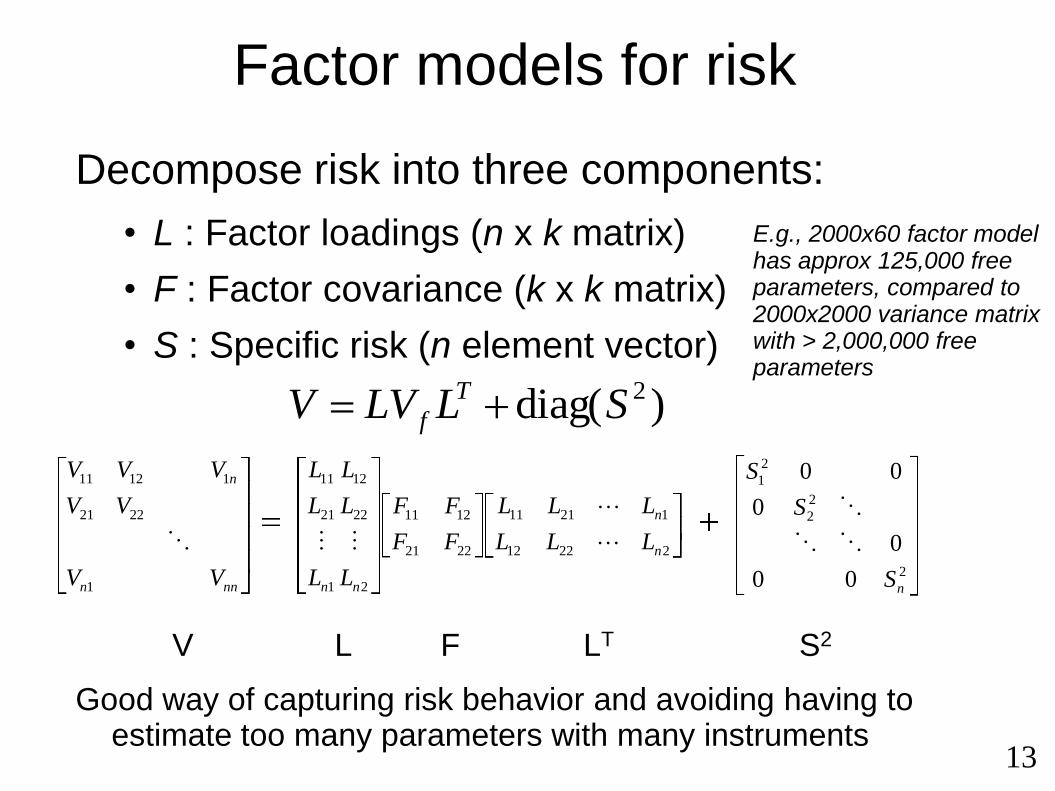
Decompose risk into three components:

• L : Factor loadings (n x k matrix)

• F : Factor covariance (k x k matrix)

• S : Specific risk (n element vector)

V L F LT S2

Good way of capturing risk behavior and avoiding having to estimate too many parameters with many instruments

)diag( 2SLLVV T

f

2

2

2

2

1

22212

12111

2221

1211

2

22

12

1

21

11

1

2221

11211

00

0

0

00

n

n

n

nnnnn

n

S

S

S

LLL

LLL

FF

FF

L

L

L

L

L

L

VV

VV

VVV

13

E.g., 2000x60 factor model has approx 125,000 free parameters, compared to 2000x2000 variance matrix with > 2,000,000 free parameters

Decomposition of factor-covariance matrix

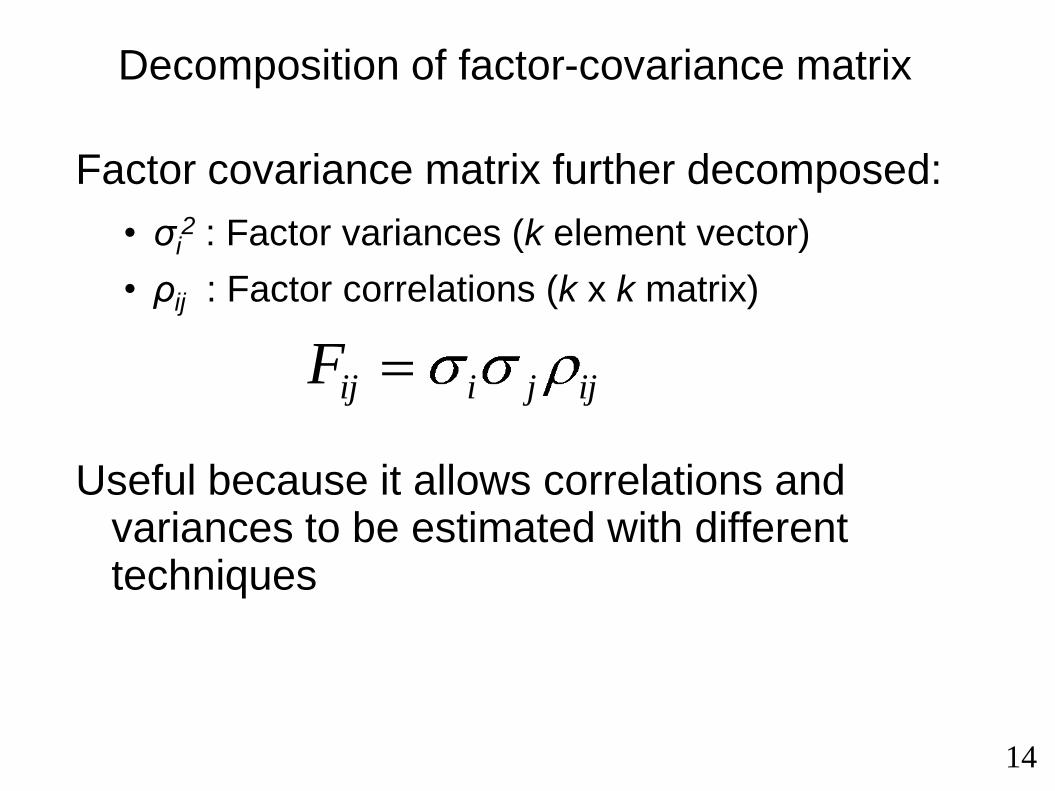
Factor covariance matrix further decomposed:

• σi2 : Factor variances (k element vector)

• ρij : Factor correlations (k x k matrix)

Useful because it allows correlations and variances to be estimated with different techniques

ijjiijF

14

Factor models & rapidly changing correlations

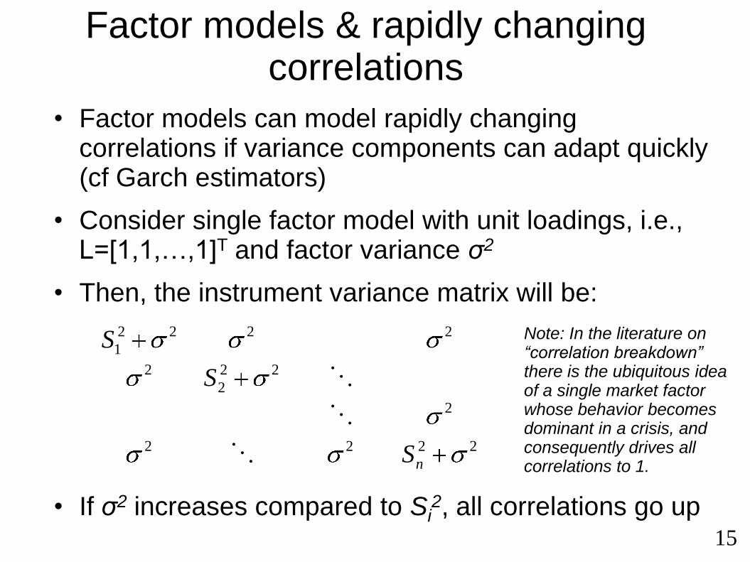
• Factor models can model rapidly changing correlations if variance components can adapt quickly (cf Garch estimators)

• Consider single factor model with unit loadings, i.e., L=[1,1,…,1]T and factor variance σ2

• Then, the instrument variance matrix will be:

• If σ2 increases compared to Si2, all correlations go up

2222

2

22

2

2

2222

1

nS

S

S

15

Note: In the literature on “correlation breakdown” there is the ubiquitous idea of a single market factor whose behavior becomes dominant in a crisis, and consequently drives all correlations to 1.

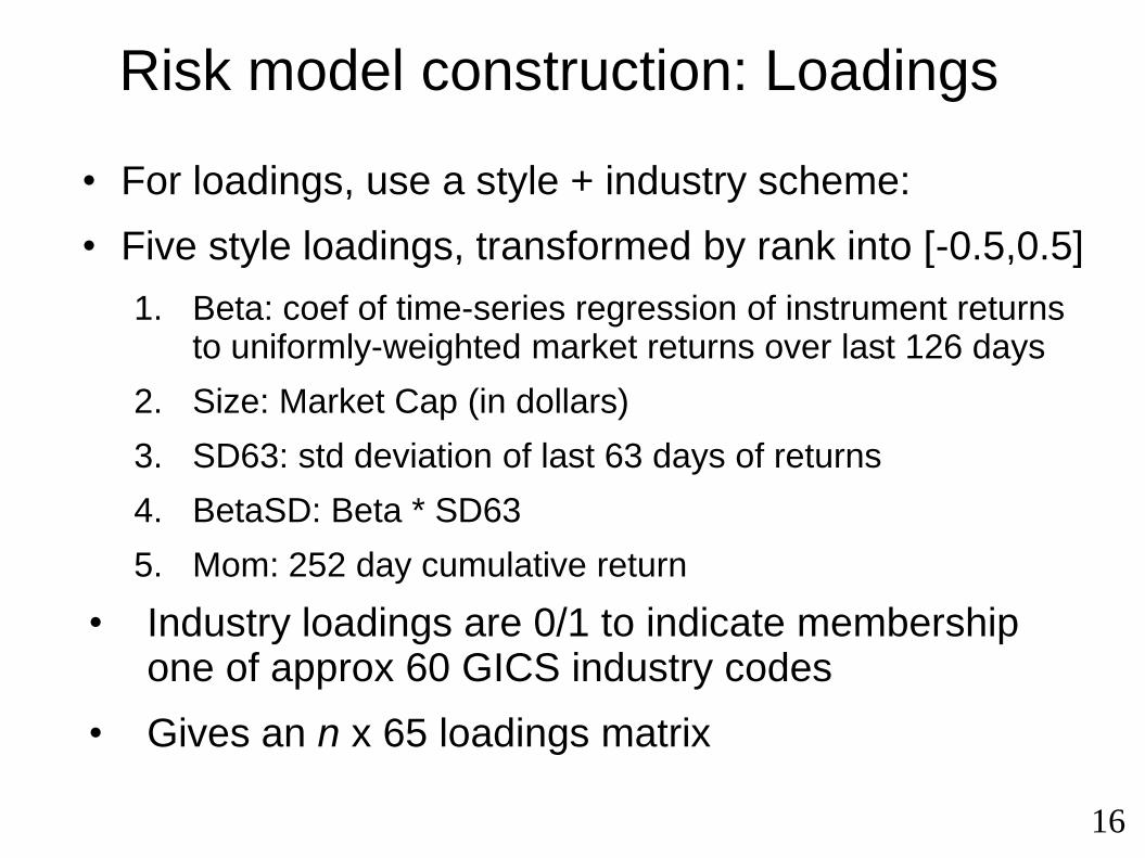
Risk model construction: Loadings

• For loadings, use a style + industry scheme:

• Five style loadings, transformed by rank into [-0.5,0.5]

1. Beta: coef of time-series regression of instrument returns to uniformly-weighted market returns over last 126 days

2. Size: Market Cap (in dollars)

3. SD63: std deviation of last 63 days of returns

4. BetaSD: Beta * SD63

5. Mom: 252 day cumulative return

• Industry loadings are 0/1 to indicate membership one of approx 60 GICS industry codes

• Gives an n x 65 loadings matrix

16

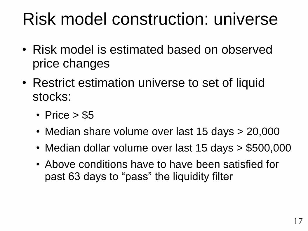
Risk model construction: universe

• Risk model is estimated based on observed price changes

• Restrict estimation universe to set of liquid stocks:

• Price > $5

• Median share volume over last 15 days > 20,000

• Median dollar volume over last 15 days > $500,000

• Above conditions have to have been satisfied for past 63 days to “pass” the liquidity filter

17

Risk model construction: Factor returns

• Factor returns computed daily by linear regression (cross-sectional) of stock returns on loadings

• is the return of stock i on day t

• is the return of factor k on day t

• is the loading for factor k of stock i on day t

• is the residual (return) for stock i on day t

• Variation: include an intercept, but as is redundant, set to: (cf Multilevel modeling)

• And then regress on loadings as above

18

titiktktittitti LRLRLRr 2211

ti

tikLtkR

tir

i tint rM 1

)( tti Mr

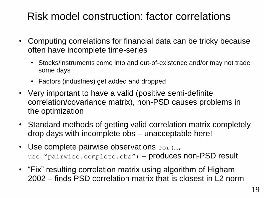
Risk model construction: factor correlations

• Computing correlations for financial data can be tricky because often have incomplete time-series

• Stocks/instruments come into and out-of-existence and/or may not trade some days

• Factors (industries) get added and dropped

• Very important to have a valid (positive semi-definite correlation/covariance matrix), non-PSD causes problems in the optimization

• Standard methods of getting valid correlation matrix completely drop days with incomplete obs – unacceptable here!

• Use complete pairwise observations cor(…, use=“pairwise.complete.obs”) – produces non-PSD result

• “Fix” resulting correlation matrix using algorithm of Higham 2002 – finds PSD correlation matrix that is closest in L2 norm

19

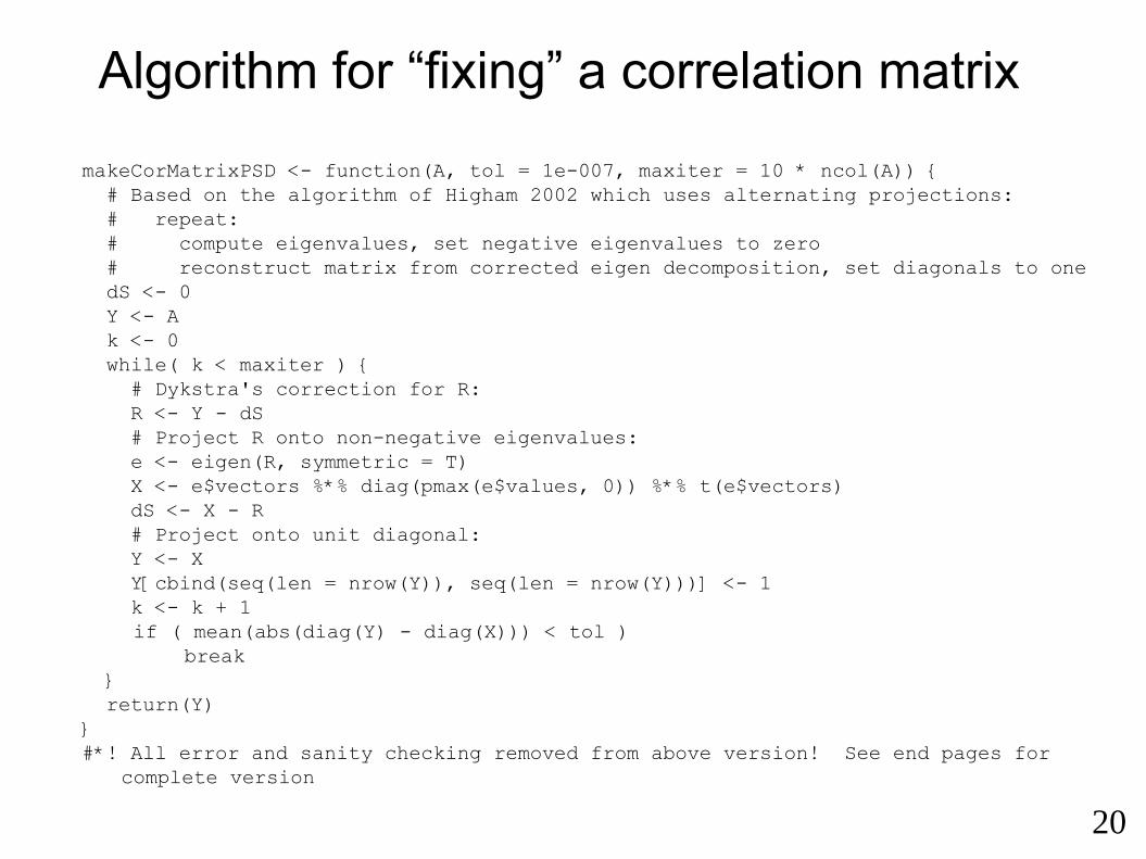
Algorithm for “fixing” a correlation matrix

makeCorMatrixPSD <- function(A, tol = 1e-007, maxiter = 10 * ncol(A)) {

# Based on the algorithm of Higham 2002 which uses alternating projections:

# repeat:

# compute eigenvalues, set negative eigenvalues to zero

# reconstruct matrix from corrected eigen decomposition, set diagonals to one

dS <- 0

Y <- A

k <- 0

while( k < maxiter ) {

# Dykstra's correction for R:

R <- Y - dS

# Project R onto non-negative eigenvalues:

e <- eigen(R, symmetric = T)

X <- e$vectors %*% diag(pmax(e$values, 0)) %*% t(e$vectors)

dS <- X - R

# Project onto unit diagonal:

Y <- X

Y[cbind(seq(len = nrow(Y)), seq(len = nrow(Y)))] <- 1

k <- k + 1

if ( mean(abs(diag(Y) - diag(X))) < tol )

break

}

return(Y)

}

#*! All error and sanity checking removed from above version! See end pages for

complete version

20

Full code for makeCorMatrixPSD()

makeCorMatrixPSD <- function(A, tol=1e-7, maxiter=10*ncol(A), verbose=FALSE) {

# Make a symmetric matrix into correlation matrix by making it

# positive semi-definite using an iterative approach.

# Return the closest PSD correlation matrix to A in terms of the Frobenius norm

# Based on the algorithm of Higham 2002 which uses alternating projections:

# repeat:

# compute eigenvalues, set negative eigenvalues to zero

# reconstruct matrix from corrected eigen decomposition, set diagonals to one

#

A.attr <- attributes(A)

if (length(dim(A))!=2 || nrow(A) != ncol(A))

stop("A must be a square matrix")

# Replace NA values with their corresponding transpose element

if (any(A.na <- is.na(A)))

A[] <- ifelse(!A.na, A, t(A))

# Replace NA diagonals with 1 and NA off-diagonals with zero

ii <- which(is.na(A), arr=TRUE)

if (nrow(ii)) {

on.diag <- ii[,1] == ii[,2]

if (any(on.diag)) A[ii[on.diag,,drop=FALSE]] <- 1

if (any(!on.diag)) A[ii[!on.diag,,drop=FALSE]] <- 0

}

# Make sure the matrix is symmetric -- otherwise can get complex eigen values

tA <- t(A)

if (any(abs(tA - A) > 0)) {

# only warn if lack of symmetry > tol (use abs tol val here because we are working

# with a correlation matrix which has a natural scale of -1/1

if (any(abs(tA - A) > tol))

warning("making non-symmetric correlation matrix symmetric")

A <- (A + tA) / 2

}

dS <- 0

Y <- A

k <- 0

while (k==0 || k < maxiter) {

# Dykstra's correction for R:

R <- Y - dS

# Project R onto non-negative eigenvalues:

e <- eigen(R, symmetric=TRUE)

X <- e$vectors %*% diag(pmax(e$values, 0)) %*% t(e$vectors)

dS <- X - R

# Project onto unit diagonal:

Y <- X

Y[cbind(seq(len=nrow(Y)), seq(len=nrow(Y)))] <- 1

k <- k+1

if (verbose)

catn("iter", k, "closeness to diag=", format(mean(abs(diag(Y) - diag(X)))))

conv <- mean(abs(diag(Y) - diag(X)))

if (conv < tol)

break

}

if (conv >= tol)

warning("failed to achieve convergence tol=", tol, " in ", k, " iterations; reached ",

format(conv))

e <- eigen(Y, symmetric=TRUE, only.values=TRUE)

attributes(Y) <- A.attr

structure(Y, psdinfo=list(convergence=(conv < tol), delta=conv, dist=sqrt(sum((A-Y)^2)),

rank=sum(abs(e$values)>tol*10), iters=k))

}

21

makeCovMatrixPSD <- function(A, tol=1e-7, maxiter=10*ncol(A), verbose=FALSE) {

dd <- diag(A)

if (any(i <- is.na(dd) | dd<=0)) dd[i] <- 1

scale <- sqrt(dd)

C <- A * outer(1/scale, 1/scale, FUN="*")

X <- makeCorMatrixPSD(C, tol=tol, maxiter=maxiter, verbose=verbose)

return(X * outer(scale, scale, FUN="*"))

}

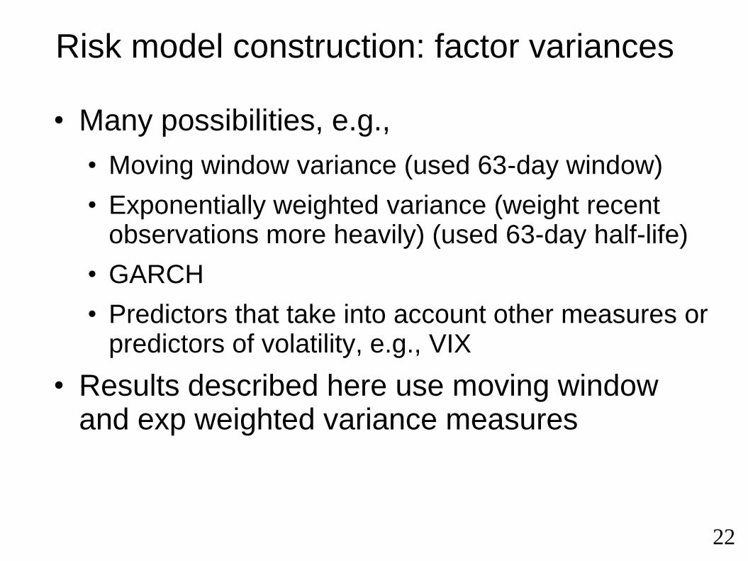
Risk model construction: factor variances

• Many possibilities, e.g.,

• Moving window variance (used 63-day window)

• Exponentially weighted variance (weight recent observations more heavily) (used 63-day half-life)

• GARCH

• Predictors that take into account other measures or predictors of volatility, e.g., VIX

• Results described here use moving window and exp weighted variance measures

22

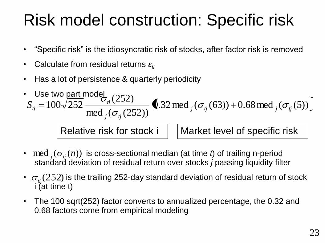
Risk model construction: Specific risk

• “Specific risk” is the idiosyncratic risk of stocks, after factor risk is removed

• Calculate from residual returns εti

• Has a lot of persistence & quarterly periodicity

• Use two part model

• is cross-sectional median (at time t) of trailing n-period standard deviation of residual return over stocks j passing liquidity filter

• is the trailing 252-day standard deviation of residual return of stock i (at time t)

• The 100 sqrt(252) factor converts to annualized percentage, the 0.32 and 0.68 factors come from empirical modeling

23

))5((med68.0))63((med32.0))252((med

)252(252100 tjjtjj

tjj

titiS

))((med ntjj

Relative risk for stock i Market level of specific risk

)252(ti

24

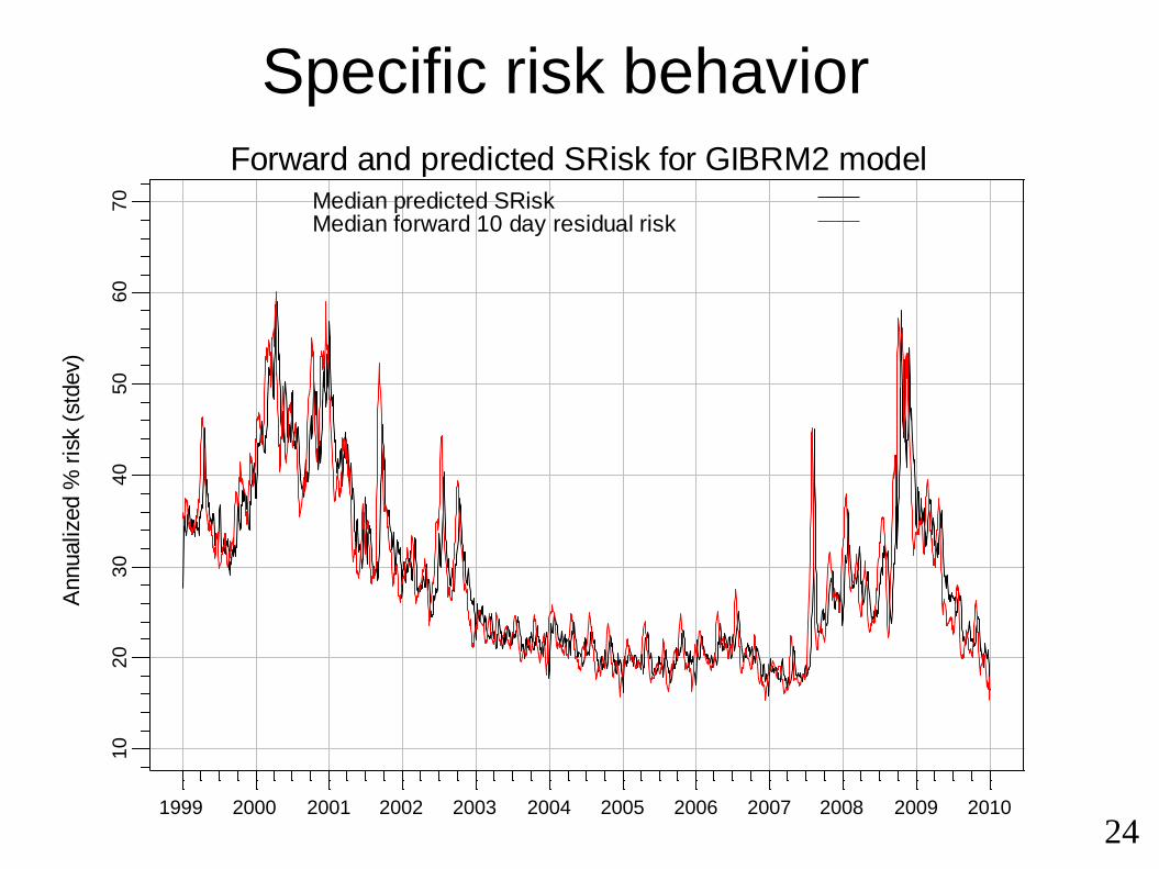
Annualized %

ris

k (

std

ev)

1999 2000 2001 2002 2003 2004 2005 2006 2007 2008 2009 2010

10

20

30

40

50

60

70

Forward and predicted SRisk for GIBRM2 modelMedian predicted SRiskMedian forward 10 day residual risk

D:/blackmesa/Research/2010-01-opt-us20 Wed Apr 14 00:16:45 MDT 2010

Specific risk behavior

251999 2000 2001 2002 2003 2004 2005 2006 2007 2008 2009 2010

-0.4

-0.2

0.0

0.2

0.4

0.6

0.8

1.0

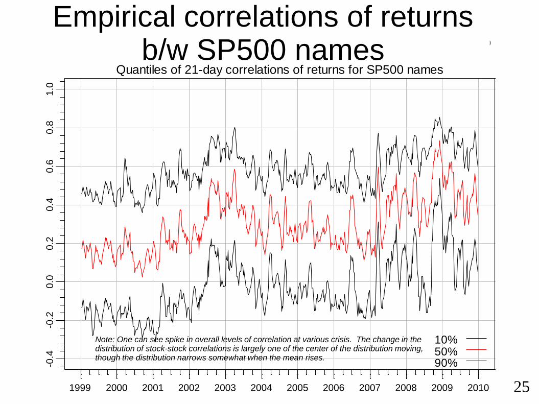
Quantiles of 21-day correlations of returns for SP500 names

10% 50% 90%


Empirical correlations of returns b/w SP500 names

Note: One can see spike in overall levels of correlation at various crisis. The change in the distribution of stock-stock correlations is largely one of the center of the distribution moving, though the distribution narrows somewhat when the mean rises.

261999 2000 2001 2002 2003 2004 2005 2006 2007 2008 2009 2010

-0.6

-0.4

-0.2

0.0

0.2

0.4

0.6

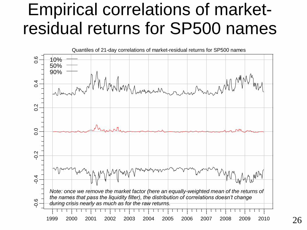
Quantiles of 21-day correlations of market-residual returns for SP500 names

10% 50% 90%


Empirical correlations of market-residual returns for SP500 names

Note: once we remove the market factor (here an equally-weighted mean of the returns of the names that pass the liquidity filter), the distribution of correlations doesn’t change during crisis nearly as much as for the raw returns.

271999 2000 2001 2002 2003 2004 2005 2006 2007 2008 2009 2010

0.0

0.1

0.2

0.3

0.4

0.5

0.6

0.7

0.8

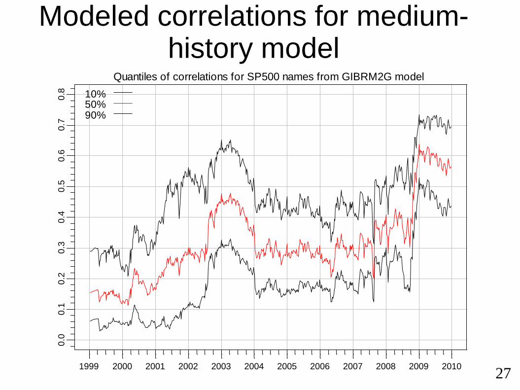
Quantiles of correlations for SP500 names from GIBRM2G model

10% 50% 90%


Modeled correlations for medium-history model

28

1999 2000 2001 2002 2003 2004 2005 2006 2007 2008 2009 2010

0.0

0.1

0.2

0.3

0.4

0.5

0.6

0.7

0.8

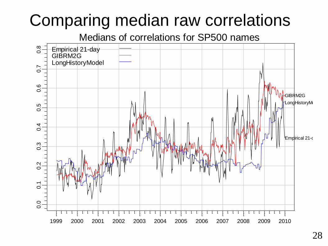
Medians of correlations for SP500 namesEmpirical 21-dayGIBRM2GLongHistoryModel

Empirical 21-day

GIBRM2G

LongHistoryModel

D:/blackmesa/Research/2010-01-opt-us20 Wed Apr 14 01:01:58 MDT 2010Comparing median raw correlations

292000 2001 2002 2003 2004 2005 2006 2007 2008 2009 2010

-0.4

-0.2

0.0

0.2

0.4

0.6

0.8

1.0

1.2

1.4

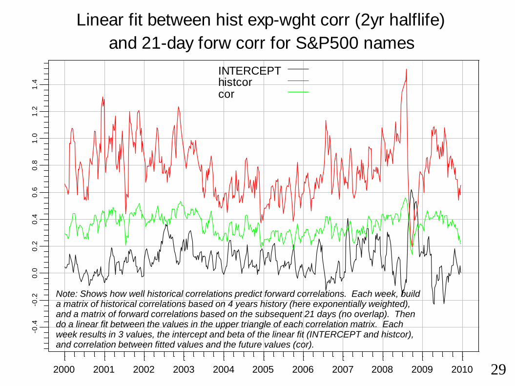
INTERCEPThistcorcor

Linear fit between hist exp-wght corr (2yr halflife)

and 21-day forw corr for S&P500 names

Note: Shows how well historical correlations predict forward correlations. Each week, builda matrix of historical correlations based on 4 years history (here exponentially weighted), and a matrix of forward correlations based on the subsequent 21 days (no overlap). Then do a linear fit between the values in the upper triangle of each correlation matrix. Each week results in 3 values, the intercept and beta of the linear fit (INTERCEPT and histcor), and correlation between fitted values and the future values (cor).

302000 2001 2002 2003 2004 2005 2006 2007 2008 2009 2010

-0.4

-0.2

0.0

0.2

0.4

0.6

0.8

1.0

1.2

1.4

INTERCEPThistcorcor

Linear fit between GIBRM2G.MR.corxw2y.uvarxw63d corr

and 21-day forw corr for S&P500 names

Note: Shows how well correlations from a risk model predict forward correlations. Each week, build a risk model matrix based on behavior of stocks that pass the liquidity filter, using 4 years of daily factor return history to calculate the factor correlation matrix (with exponential weighting with a half life of 2 years) and exponentially weighted factor variance estimates (half life 63 days). From the risk model, construct a stock-stock correlation matrix for S&P500 names. Also construct a matrix of forward stock-stock correlations based on the subsequent 21 days (no overlap). Then do a linear fit between the values in the upper triangle of each correlation matrix. Each week results in 3 values, the intercept and beta of the linear fit (INTERCEPT and histcor), and correlation between fitted values and the future values (cor).

Optimization experiments

• Report optimization experiments using a variety of risk models

• Use period 2000-2009, S&P 500 stocks for optimization

• Rebalance each portfolio every 5 business days, calculate PnL every day

• Always use causally valid risk models – for optimizing portfolio at any time, risk model is built from data available strictly before then

• Risk model estimated on a universe of the most liquid US stocks (exact number varies over time, typically between 1500 and 2000 names pass the liquidity filter)

• Look at performance in “normal” (2003 thru 08) periods vs the crisis of 2008/09 (Sept 08 thru Mar 09)

• To understand whether performance differences are meaningful, use random subset portfolios

• Evaluate PnL for an optimized portfolio constructed from each of 200 random subsets (2/3) of the S&P500

31

Variations of risk models

• Simple schemes:• UPf: uniform weight portfolio

• TRisk1: weight of a name is prop to inverse of total risk (variance)

• Loadings:• MKTRMG: Intercept only

• BBRM2G: Beta factor + Intercept

• GIBRM2G: 5 style factors, approx 60 industries

• GIBRM2OG: like GIBRM2G, but factors mutually orthogonalized each week (first make

industries zero-mean, then orthogonalize remaining factors to industries, and make them

mutually orthogonal)

• Factor return fitting technique:• MR: use Intercept together with industry membership factors, set to mean return

(MR=“market residual”)

• VN: no Intercept (VN=“Vanilla”) (when used with industry membership factors)

• Correlation matrix technique:• cor: 2 year moving window

• corxw: 4 year moving window with exponential weighting with 2-year half life

• coraz: off-diagonal elements are zero (to remove dependence on historical correaltions)

• Factor variance technique• uvar: 63-day moving window

• uvarxw: 126-day moving window with exponential weighting with 63-day half-life

32

33

log r

etu

rn

2000 2001 2002 2003 2004 2005 2006 2007 2008 2009 2010

-1.0

-0.5

0.0

0.5

1.0

1.5

Compounded PnL for full S&P500 universe

BBRM2G.MR.corxw2y.uvar63dGIBRM2G.MR.corxw2y.uvar63dTRisk1UPfSPX

BBRM2G.MR.corxw2y.uvar63d

GIBRM2G.MR.corxw2y.uvar63dTRisk1

UPf

SPX


34

log r

etu

rn

2000 2001 2002 2003 2004 2005 2006 2007 2008 2009 2010

-0.2

0.0

0.2

0.4

0.6

0.8

1.0

1.2

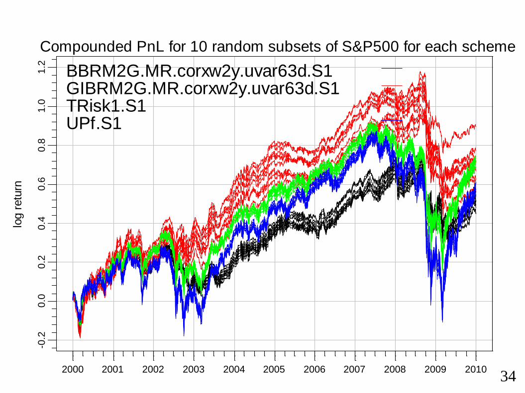
Compounded PnL for 10 random subsets of S&P500 for each scheme

BBRM2G.MR.corxw2y.uvar63d.S1GIBRM2G.MR.corxw2y.uvar63d.S1TRisk1.S1UPf.S1


352000 2001 2002 2003 2004 2005 2006 2007 2008 2009 2010

0.5

1.0

1.5

2.0

2.5

3.0

3.5

4.0

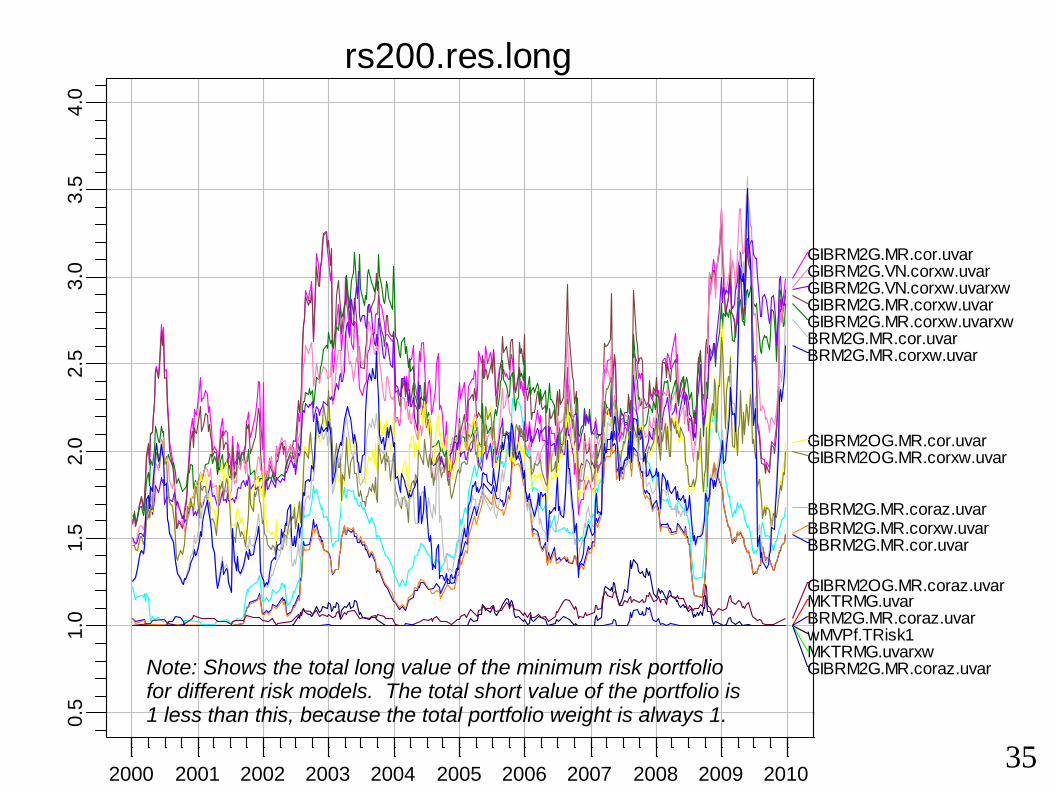
rs200.res.long

wMVPf.TRisk1

MKTRMG.uvar

MKTRMG.uvarxw

BBRM2G.MR.cor.uvarBBRM2G.MR.corxw.uvarBBRM2G.MR.coraz.uvar

GIBRM2G.MR.cor.uvar

GIBRM2G.MR.corxw.uvarGIBRM2G.MR.corxw.uvarxw

GIBRM2G.MR.coraz.uvar

GIBRM2G.VN.corxw.uvarGIBRM2G.VN.corxw.uvarxw

GIBRM2OG.MR.cor.uvarGIBRM2OG.MR.corxw.uvar

GIBRM2OG.MR.coraz.uvar

BRM2G.MR.cor.uvarBRM2G.MR.corxw.uvar

BRM2G.MR.coraz.uvar

D:/blackmesa/Research/2010-01-opt-us20 Thu Apr 15 10:37:51 MDT 2010

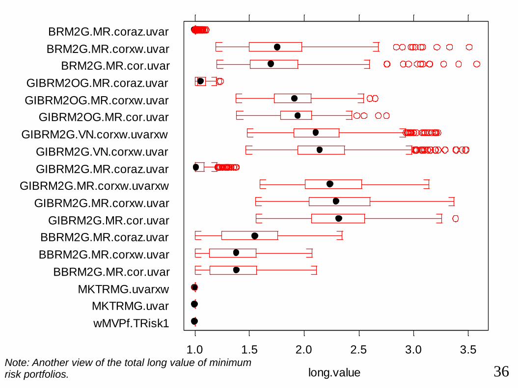
Note: Shows the total long value of the minimum risk portfolio for different risk models. The total short value of the portfolio is 1 less than this, because the total portfolio weight is always 1.

36

wMVPf.TRisk1

MKTRMG.uvar

MKTRMG.uvarxw

BBRM2G.MR.cor.uvar

BBRM2G.MR.corxw.uvar

BBRM2G.MR.coraz.uvar

GIBRM2G.MR.cor.uvar

GIBRM2G.MR.corxw.uvar

GIBRM2G.MR.corxw.uvarxw


GIBRM2G.VN.corxw.uvar

GIBRM2G.VN.corxw.uvarxw

GIBRM2OG.MR.cor.uvar

GIBRM2OG.MR.corxw.uvar


BRM2G.MR.cor.uvar

BRM2G.MR.corxw.uvar

BRM2G.MR.coraz.uvar

1.0 1.5 2.0 2.5 3.0 3.5

long.valueNote: Another view of the total long value of minimum risk portfolios.

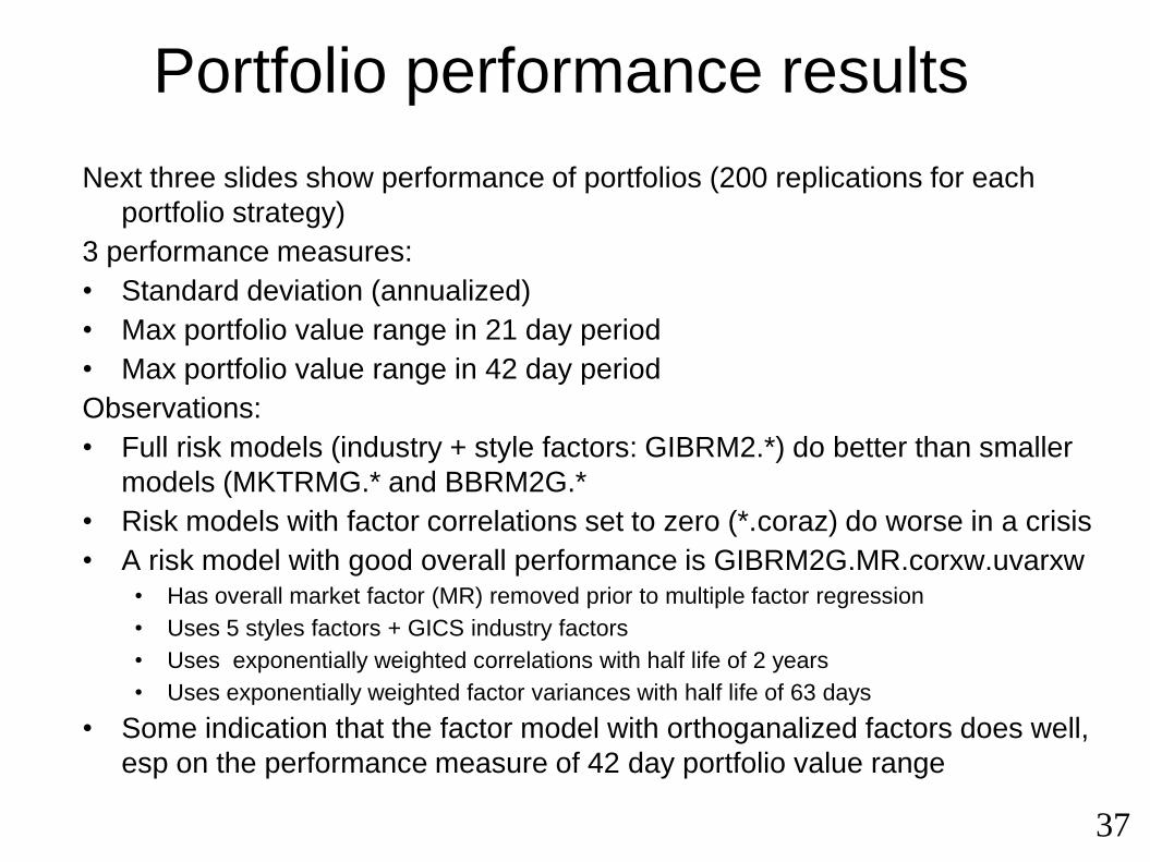
Portfolio performance results

Next three slides show performance of portfolios (200 replications for each

portfolio strategy)

3 performance measures:

• Standard deviation (annualized)

• Max portfolio value range in 21 day period

• Max portfolio value range in 42 day period

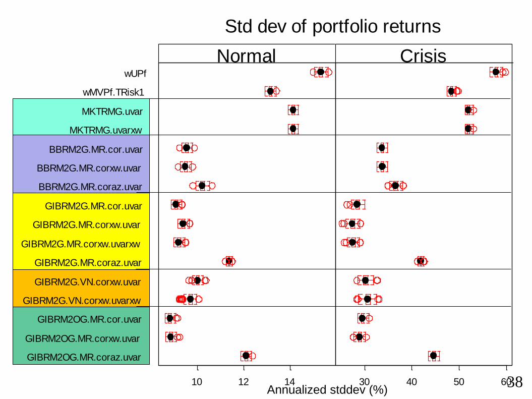
Observations:

• Full risk models (industry + style factors: GIBRM2.*) do better than smaller

models (MKTRMG.* and BBRM2G.*

• Risk models with factor correlations set to zero (*.coraz) do worse in a crisis

• A risk model with good overall performance is GIBRM2G.MR.corxw.uvarxw• Has overall market factor (MR) removed prior to multiple factor regression

• Uses 5 styles factors + GICS industry factors

• Uses exponentially weighted correlations with half life of 2 years

• Uses exponentially weighted factor variances with half life of 63 days

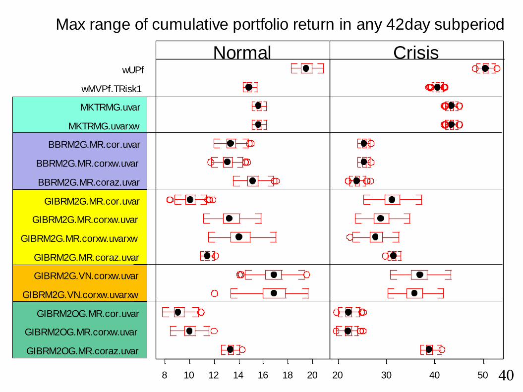
• Some indication that the factor model with orthoganalized factors does well,

esp on the performance measure of 42 day portfolio value range

37

38









GIBRM2G.MR.cor.uvar



BBRM2G.MR.cor.uvar

MKTRMG.uvarxw

MKTRMG.uvar

wMVPf.TRisk1

wUPf

10 12 14

Normal

30 40 50 60

Crisis

Annualized stddev (%)

Std dev of portfolio returns

Annualized stddev (%)

39









GIBRM2G.MR.cor.uvar



BBRM2G.MR.cor.uvar

MKTRMG.uvarxw

MKTRMG.uvar

wMVPf.TRisk1

wUPf

8 10 12 14 16

Normal

20 25 30 35

Crisis

(%)

Max range of cumulative portfolio return in any 21day subperiod

(%)









GIBRM2G.MR.cor.uvar



BBRM2G.MR.cor.uvar

MKTRMG.uvarxw

MKTRMG.uvar

wMVPf.TRisk1

wUPf

8 10 12 14 16 18 20

Normal

20 30 40 50

Crisis

(%)

Max range of cumulative portfolio return in any 42day subperiod

40

Conclusions

• Initial goal was to show that correlations are so unstable in a crisis that it was better to ignore them all the time

• Minimum Variance Portfolios for S&P500 equities based on optimizing with a factor model showed:

• Ignoring correlations doesn’t help

• A model based on historical correlations does better than simple alternatives

• Maybe the emperor is at least wearing underpants, after all

41

mean-variance portfolio optimization: do historical...

Documents