Meaning and DualityFrom Categorical Logic to Quantum Physics

Yoshihiro Maruyama

Wolfson College

University of Oxford

A thesis submitted for the degree of

Doctor of Philosophy

Trinity 2016

[A]dvances forged by category theorists will be of value to [..]

philosophy, lending precise form [..] to ancient philosophical

distinctions such as [..] objective vs. subjective, being vs.

becoming, space vs. quantity [..] (William Lawvere, 1992)

Myth and art, language and science, are in this sense shap-

ings toward being; they are not simple copies of an already

present reality, but they rather present the great lines of

direction of spiritual development, of the ideal process, in

which reality constitutes itself for us as one and many – as a

manifold of forms, which are nonetheless finally held together

by a unity of meaning. (Ernst Cassirer, 1923; translation by

Michael Friedman in his A Parting of the Ways)

To my family.

Acknowledgements

Above all, I would like to express my gratitude to my supervisors Samson

Abramsky (“Samson the Dinosaur”) and Bob Coecke (“Failed Artist”)

for everything including their guidance, encouragement, and inspiration

generously given to me throughout my D.Phil. Notwithstanding that I

surely acquired a substantial amount of knowledge from their high level

of expertise, I nevertheless learned even more from their “backs”, the very

ways they live as human beings, of two very distinct kinds, I would say.

Mathematical thanks go to Hilary Priestley for duality discussions and

for her kindly accepting the role of an examiner in my D.Phil. transfer

viva. Philosophical thanks go to Peter Schroeder-Heister for the theory of

meaning discussions during his sabbatical visit to Oxford, which influenced

the conceptual underpinning of the thesis including the title per se. More

broadly, I am greatly indebted to Klaus Keimel for his gentle continual

support, and also for strong letters of recommendation for my applications

to Oxford and elsewhere. Besides, I would like to thank Kentaro Sato for

telling me how to do research in the first place when I was just a third-

year undergrad, and for the massive amount of discussions we have had

since. Last, but not least, I would like to thank the members of the Oxford

School of Quantum Foundations and of Wolfson College (aka. “Quantum

College”); to name just a few, Chris Heunen and Jamie Vicary were gentle

enough to serve as examiners for my transfer/confirmation viva.

All in all, the amount of support I have got is overwhelming, notwithstand-

ing that I have attempted to be mostly independent of people in my life.

I do not know how to reward it. Perhaps the best way to do so, I believe,

would be my contributing to the mankind’s system of knowledge as much

as possible through scholarly work in my remaining life, whether long or

short. And only by doing so could I really appreciate their graciousness.

I hereby acknowledge financial and other support during my D.Phil. from:

the Nakajima Foundation; Wolfson College; the University of Oxford.

Abstract

Duality abounds in science, both pure and applied: in mathematics there

is duality between space and algebra; in physics there is duality between

states and observables; in information science there is duality between sys-

tems and properties/behaviours; in logic there is duality between models

and theories; and even in philosophy there is duality between realism and

antirealism (Dummett), or substance metaphysics and process/function

metaphysics (Whitehead/Cassirer). They look akin at a level of abstrac-

tion, and yet, taking a closer look at subtleties involved, one may find a

parting of the ways. The present thesis builds upon category theory and

universal algebra to explicate and articulate the dynamics of duality, the

mechanism of how duality emerges, changes, and breaks. A generic duality

theory is first pursued in the abstract via categorical topology and algebra,

and subtler duality theories are then explored to the end of shedding light

on more nuanced facets of concrete dualities such as coalgebraic dualities.

Each duality theory thus developed is cashed out to uncover formerly un-

known dualities; e.g., the first duality theory tells us a dual equivalence

between domains and convex structures, which remained an open problem

before. Dualities are often induced by Janusian objects, which sometimes

form truth value objects as in topos theory. To elucidate this link between

duality and categorical logic, categorical universal logic is developed on

the basis of Lawvere’s hyperdoctrine and Hyland-Johnstone-Pitts’ tripos,

thereby expanding the realm of (first-order/higher-order) categorical logic

so as to encompass, inter alia, classical, intuitionistic, quantum, fuzzy,

relevant, and linear logics. Finally, duality meets symmetry in quantum

physics, yielding a categorical understanding of the Wigner theorem, i.e.,

a purely coalgebraic characterisation of the quantum symmetry groupoid.

In passing, operational quantum duality is systematised via Chu space

theory. In light of these, duality would arguably serve as a unifying prin-

ciple to overcome the fragmentation of science, and to soothe the dualistic

divide of philosophy between realist and antirealist worldviews.

Contents

1 Introduction 2

1.1 Dualism . . . . . . . . . . . . . . . . . . . . . . . . . . . . . . . . . . 2

1.2 Duality . . . . . . . . . . . . . . . . . . . . . . . . . . . . . . . . . . . 5

1.3 Disduality . . . . . . . . . . . . . . . . . . . . . . . . . . . . . . . . . 8

1.4 Synopsis . . . . . . . . . . . . . . . . . . . . . . . . . . . . . . . . . . 10

2 Categorical Duality 17

2.1 Introduction to the Chapter . . . . . . . . . . . . . . . . . . . . . . . 17

2.2 Duality Theory via Categorical Topology and Algebra . . . . . . . . . 21

2.2.1 A Categorical Conception of Point-Set Spaces . . . . . . . . . 22

2.2.2 Dual Adjunction via Harmony Condition . . . . . . . . . . . . 25

2.3 Domain-Convexity Duality . . . . . . . . . . . . . . . . . . . . . . . . 33

2.3.1 Convexity-Theoretical Duality for Scott’s Continuous Domains 33

2.3.2 Jacobs Duality for Algebras of the Distribution Monad . . . . 36

2.4 Categorical Duality as Philosophy of Space . . . . . . . . . . . . . . . 40

3 Articulating Duality 48

3.1 Introduction to the First Part . . . . . . . . . . . . . . . . . . . . . . 48

3.2 The Notion of ISPM and the Kripke Condition . . . . . . . . . . . . . 52

3.3 Modal Semi-Primal Duality . . . . . . . . . . . . . . . . . . . . . . . 56

3.4 Coalgebraic Duality and its Applications . . . . . . . . . . . . . . . . 68

3.5 Introduction to the Second Part . . . . . . . . . . . . . . . . . . . . . 73

3.6 The Notion of Topological Dualisability . . . . . . . . . . . . . . . . . 77

3.7 Non-Hausdorff Stone Duality and its Applications . . . . . . . . . . . 78

3.8 Mathematical and Philosophical Remarks . . . . . . . . . . . . . . . . 94

i

4 Duality and Categorical Logic 100

4.1 Introduction to the First Part . . . . . . . . . . . . . . . . . . . . . . 101

4.2 Typed Full Lambek Calculus and Full Lambek Hyperdoctrine . . . . 105

4.3 Hyperdoctrinal Girard and Godel Translation . . . . . . . . . . . . . 119

4.4 Higher-Order Full Lambek Calculus and Full Lambek Tripos . . . . . 120

4.5 Tripos-Theoretical Girard and Godel Translation . . . . . . . . . . . 130

4.6 Introduction to the Second Part . . . . . . . . . . . . . . . . . . . . . 133

4.7 Categorical Universal Logic . . . . . . . . . . . . . . . . . . . . . . . 136

4.8 Duality as Categorical Semantics . . . . . . . . . . . . . . . . . . . . 142

4.9 Geometric Logic, Convexity Logic, and Quantum Logic, Categorically 150

4.10 Lawvere-Tierney Topology as Logical Translation . . . . . . . . . . . 156

4.11 Remarks on Duality in Logic and Algebraic Geometry . . . . . . . . . 161

5 Duality and Quantum Physics 166

5.1 Introduction to the Chapter . . . . . . . . . . . . . . . . . . . . . . . 166

5.2 Duality and Chu Space Representation . . . . . . . . . . . . . . . . . 169

5.2.1 Chu Representation of Quantum Systems . . . . . . . . . . . . 170

5.2.2 Chu Theory of T1-Type Dualities via Closure Conditions . . . 172

5.3 Quantum Symmetries and Closure-Based Coalgebras . . . . . . . . . 183

5.3.1 Born Coalgebras on Closure Spaces . . . . . . . . . . . . . . . 184

5.3.2 Quantum Symmetries Are Purely Coalgebraic . . . . . . . . . 186

5.4 Remarks on the Duality of Reproducing Kernel Hilbert Spaces . . . . 191

6 Conclusions and Prospects 197

6.1 How Duality Emerges, Changes, and Breaks . . . . . . . . . . . . . . 197

6.2 A Bird’s-Eye View of Stone Dualities . . . . . . . . . . . . . . . . . . 199

6.3 The Disclosure of Meaning . . . . . . . . . . . . . . . . . . . . . . . 201

A Scheme-Theoretical Duality Theory 207

B Duality, Modality, and Vagueness 224

C Artificial Intelligence Applications 250

Bibliography 266

ii

Chapter 1

Introduction

The major concern of the present thesis lies in elucidating the dynamics of duality

through the exploration of the way how duality emerges, changes (and breaks). A

direct answer to the question shall be given in the concluding chapter. In this in-

troductory chapter let us start the discussion with a conceptual account of dualism,

duality, and disduality in the abstract; disduality is basically meant to be the absence

of duality, or duality-breaking. Dualism and duality are related to each other, and yet

surely different (how they are different is not that obvious, though). The following

account of the three concepts would be slightly lengthy, and so, if the reader in

a rush would rather like to have a quick bird’s-eye view of the thesis, it

would be advised to skip the entire discussion on dualism, duality, and

disduality, and immediately proceed to the synopsis Section 1.4 below, in

which everything you would practically need to know about the thesis, including a

rough picture of technicalities involved, is explained as briefly as possible.

1.1 Dualism

Developments of philosophy have centred around a tension between realism and an-

tirealism (or in Godel’s tems between the “right” and the “left”; see Godel’s amusingly

bold, philosophical article entitled “The modern development of the foundations of

mathematics in the light of philsoophy” [113], which shall be discussed later). And the

dualistic tension may be illustrated by asking the nature of a variety of fundamental

concepts. What is Meaning? The realist asserts it consists in the correspondence of

language to reality, whilst the antirealist contends it lies in the autonomous system or

internal structure of language or linguistic practice (cf. the early Wittgenstein [279]

vs. the later Wittgenstein [280]; Davidson [75] vs. Dummett [87]). What is Truth?

To the realist, it is the correspondence of assertions to facts or states of affairs; to

2

the antirealist, it has no outward reference, constituted by the internal coherency

of assertions or by some sort of instrumental pragmatics (cf. Russell vs. Bradley

[49]). What is Being? To the realist, it is persistent substance; to the antirealist, it

emerges within an evolving process, cognition, structure, network, environment, or

context (cf. Aristotle [16] vs. Cassirer/Heidegger/Whitehead [52, 131, 277]). What

is Intelligence? To the realist, it is more than behavioural simulation, characterised

by the intentionality of mind; to the antirealist, it is fully conferred by copycatting

as in the Turing test or the Chinese Room (cf. Searle [250] vs. Turing [268]). What

is Space? To the realist, it is a collection of points with no extension; to the antire-

alist, it is a structure of regions, relations, properties, or information (cf. Newton vs.

Leibniz [269]; Cantor/Russell vs. Husserl/Whitehead [28]). To cast these instances

of dualism in more general terms, dualism may be conceived of as arising between

the epistemic and the ontic, or between the formal and the conceptual in Lawvere’s

terms [171], as in the figure below:

Ontic EpistemicDescartes Matter Mind Cartesian Dualism

Kant Thing-in-itself Appearance IdealismCassirer Substance Function Logical Idealism

Heidegger Essence Existence Analysis of DaseinWhitehead Reality Process Holism/Organicism

Wittgenstein World Language Logical PhilosophySearle Intentionality Simulatability Philosophy of Mind

Dummett Truth Verification Theory of Meaning

The best known dualism would presumably be the Cartesian dualism between mind

and matter (or mind and body), in which the ontic realm of matter and the epis-

temic realm of mind are separated. The Kantian dualism between thing-in-itself and

appearance can readily be seen as a case of the ontic-epistemic dualism. Cassirer,

the logical Neo-Kantian of the Marburg School, asserted the priority of the func-

tional over the substantival [52], having built a purely functional, genetic view of

knowledge, which was mainly concerned with modern science at an early stage of his

thought as in Substance and Function [52], and yet eventually evolved to encompass

everything including humanities in his mature Philosophy of Symbolic Form [53]. It

is an all-encompassing magnificent Philosophy of Culture [178], indeed subsuming

myth, art, language, humanities, and both empirical and exact sciences. Cassirer

now counts as a precursor of what is called Structural Realism [97, 165, 166]. Yet

3

his functionalist philosophy would better be characterised as Higher-Order Structural

Realism, allowing for structures of structures (or abstraction of abstraction in a cer-

tain sense), just as in category theory. His genetic view even payed due attention to

the process of how structures are generated, just as in type theory. In light of this,

Cassirer’s philosophy may be regarded as a conceptual underpinning of the enterprise

of category theory, and his dichotomy between substance and function as that of cat-

egorical duality, which constitutes the subject matter of the present thesis. Cassirer

actually started his career with work on Leibniz and his relationalism [51], at which

we shall have a glance in the following.

Mathematially, the ontic-epistemic duality is best recognised in the nature of space

aforementioned. There were two conceptions of space at the dawn of mathematical

science: the Newtonian realist conception of absolute space and the Leibnizian antire-

alist conception of relational space [269]. Hundreds of years later, Whitehead [277]

recognised a similar tension between point-free space and point-set space (as part

of his inquiry into Process and Reality), advocating the latter point-free conception,

which may also be found in the phenomenology of Brentano and Husserl as well (see

[28]). On the one hand, points are recognition-transcendent entities (just like prime

ideals/filters, maximally consistent theories, or what Hilbert called ideal elements;

recall that the algebraic geometer indeed identify points with prime ideals, which, in

general, only exist with the help of the axiom of choice or some indeterministic princi-

ple like that). On the other, regions (or any other aforementioned entities) are more

recognition-friendly and epistemically better grounded (just as point-free topology

can be developed constructively or even predicatively in the formal topology style).

In general, realism and antirealism are grounded upon the ontic and the epistemic,

respectively.

As shown in the figure, quite some major philosophers, whether in the analytic or

continental tradition, have wondered about versions of the ontic-epistemic dualism.

The fundamental problem of such a dualism is to account for how the two different

realms can interact with each other; in the particular case of the Cartesian dualism,

it boils down to explicating how the mind can know about the material world when

they are totally (and so causally) separated. How can they causally interact at all

when they are causally separated? It appears impossible; this is the typical way the

philosopher gets troubled by dualism in accounting for the ontic-epistemic interaction.

Philosophy of mathematics faces an instance of the interaction problem as well.

If the realm of mathematical objects and the realm of human existence are totally

separated (in particular causally separated), how can human beings get epistemic

4

access to mathematical entities? If mathematical objects exist in a Platonic uni-

verse, as in Godel’s realist philosophy for example, it seems quite hard to account

for how it is possible to have a causal connection between humans in the ordinary

universe and mathematical entities in the Platonic universe when the two universes

are causally disconnected (this sort of problem is known as the Benacerraf’s dilemma

[31]). Yet if mathematical objects exist in the mind, as in Brouwer’s antirealist philos-

ophy (he counts as an antirealist at least in the sense of Dummett [87]), the account

of interaction between the ontic and the epistemic is much easier, since the ontic is,

just by assumption, reduced to the epistemic in this case; by contrast, then, it gets

harder to account for the existence and objectivity of mathematical entities, especially

transfinite ones. For instance, how can humans mentally construct far-reaching trans-

finite entities and does everyone’s mental construction really yield the same results

for sure? (To remedy the existence problem, Brouwer actually endorsed arguably

non-constructive principles. Otherwise a continuum can be countable as in recursive

mathematics in the Russian tradition; recall that the number of computable reals are

only countably many.) Summing up, realist ontology makes it difficult to account

for the possibility of epistemic access to mathematical objects; conversely, antirealist

epistemology yields ontological difficulties in constructively justifying their existence

and objectivity.

A moral drawn from the above discussion is that there is a trade-off between

realism and antirealism: straightforward realist ontology leads to involved episte-

mology with the urgent issue of epistemic access to entities unable to exist in our

ordinary, tangible universe; and straightforward antirealist epistemology to involved

ontology with the compelling problem of securing their existence and objectivity. In

general, realism gets troubled by our accessibility to abstract entities; antirealism

faces a challenge of warranting their existence and objectivity. Put simply, an easier

ontology of something often makes its epistemology more difficult, and vice versa.

Something seems reversed between realist/ontological and antirealist/epistemological

worldviews. And this is where the idea of duality between realism and antirealism

comes into the play.

1.2 Duality

Everything, from Truth and Meaning to Being and Mind, has dual facets as aforemen-

tioned. Conceptually, duality theory, in turn, is an attempt to unite them together

with the ultimate aim of showing that they are the two sides of one and the same coin.

5

Put another way, duality allows two things opposed in dualism to be reconciled and

united as just two different appearances of one and the same fundamental reality; in

this sense, duality is a sort of monism established on the top of dualism (cf. Hegelian

dialectics as in Lawvere’s philosophy of mathematics). In Dummett’s philosophy on

the theory of meaning, for example, he makes a binary opposition between realism

and antirealism (cf. Platonism and Intuitionism/Constructivism); what is at stake

there is basically the legitimacy of recognition-transcendent truth conditions, which

is allowed in realism, but not in antirealism. As shall be discussed later (and also

in the author’s philosophically oriented articles [199, 201]), however, the realist and

antirealist conceptions of meaning may be reconciled and united as sharing the same

sort of structure, even if they are literally opposed. In view of Dummett’s constitution

thesis, according to which the content of metaphysical (anti)realism is constituted by

semantic (anti)realism [87, 206], this would arguably count as a unification of meta-

physics as well as the theory of meaning. Duality thus conceived is a constructive

canon to deconstruct dualism as it were.

Whilst having posed the Cartesian dualism as aforementioned, Descartes also de-

veloped analytic geometry, which is in a sense a precursor of duality between algebra

and geometry, even though he might not have been aware that systems of equa-

tions are dual to spaces of their zero loci (logically paraphrasing, this amounts to the

fact that systems of axioms are dual to spaces of their models; and such correspon-

dence between logic and algebraic geometry can be made precise in duality theory).

Notwithstanding that Galois theory may be seen as an instance of duality, Galois

himself would not have been aware of the essentially categorical duality underpinning

his theory, either. It would, then, be Riemann who first discovered duality between

geometry and algebra in a mathematically substantial form; indeed he showed how

to reconstruct (what are now called) Riemann surfaces from function fields, and vice

versa, thereby establishing the (dual) equivalence between them. Even earlier than

Riemann, however, Dedekind-Weber and Kronecker (mathematically) gave a purely

algebraic conception of space, a sort of precursor of what is now called point-free

geometry (philosophically, it would date back to Leibniz as aforementioned).

The history of duality in mathematical form, thus, goes back to the late 19th

century (it ought to be noted here that duality in mathematical form basically means

categorically representable duality in the present thesis, and so duality in projective

geometry, for example, does count as an origin of duality in this sense; it would not be

categorically representable, at least to my knowledge). Duality then flourished in the

early 20th century, as exemplified by Hilbert’s, Stone’s, Gelfand’s, and Pontryagin’s

6

dualities (Hilbert’s Nullstellensatz is essentially a dual equivalence between finitely

generated reduced k-algebras and varieties over k for an algebraically closed field

k). The discovery of dualities was thereafter followed by applications to functional

analysis, general topology, and universal algebra on the one hand, and to algebraic

geometry, representation theory, and number theory on the other (interestingly, the

Pontryagin duality plays a vital role in number theory as exemplified by Andre Weil’s

Basic Number Theory [274]). And it was eventually accompanied by the rise of cate-

gorical language in the late 20th century, which, in particular, allowed one to identify

a universal form of duality (before category theory it was only vaguely understood

what exactly different dualities have in common, and no one was able to spell out

what presicely duality is). Today there are a great variety of dualities found across

quite different kinds of science as in the following figure (and even in engineering such

as optimisation, linear programming, control theory, and electrical circuit theory; du-

ality thus goes far beyond pure mathematics, and it may sometimes be of genuine

practical use as in those engineering theories):

N

N N

N

OPO

OHO

OH OH

PO

OHO P

O

OHOHO

Origins of DualityYoshihiro Maruyama (Hakubi the 6th batch, School of Letters, KU)

2016年度白眉年次報告会, Hakubi Annual Research Report, 研究の「原点」

Ontic EpistemicComplex Geometry Complex Surface Function Field RiemannAlgebraic Geometry Variety/Scheme k-Algebra/Ring Hilbert-Grothendieck

Galois Theory (Profinite) G-Set Algebra Extension GaloisRepresentation Th. Compact Group Representations Pontryagin-Tannaka

Anabelian Geometry Elliptic Curve Frobenioid MochizukiTopology Topological Space Algebra of Opens Isbell-Papert

Convex Geometry Convex Space Semantic Domain MaruyamaLogic Space of Models Algebra of Theories Gödel-Stone

Computer Science System Observable Properties Abramsky-SmythSystem Scicence Controllability Observability KalmanQuantum Physics State Space Alg. of Observables von NeumannGeneral Relativity Spacetime Manifold Vector Field Weyl

Descartes Matter Mind Cartesian DualismKant Thing-in-itself (Cognitive) Appearance Idealism

Cassirer Substance (Relational) Function Logical IdealismHeidegger Essence (Contextual) Existence Analysis of DaseinWhitehead Reality Process Holism/Organicism

Wittgenstein World Language Logical PhilosophySearle Intentionality Simulatability Philosophy of Mind

Dummett Truth Condition Verification Condition Theory of MeaningWhat is it all about? Everything, from Logic and Space to Meaning and Truth, has dual facets; Duality Theory in turn unites them together, thereby telling us they are the two sides of the same coin. Duality thus conceived is a constructive canon to deconstruct dualism. References: see, e.g., my articles in books Advances in Proof-Theoretic Semantics and Fundamental Issues of Artificial Intelligence, both from Springer, and 『圏論の歩き方』.

These dualities are diverse at first sight, and yet tightly intertwined with each other in

their conceptual structures. To pursue links between different dualities is indeed one

of the principal aims of duality theory. Since duality, as opposed to dualism and disd-

uality, is the major concern of the thesis, more specialised discussions on some part of

the picture above shall be continued and elaborated in the outline of the thesis below.

It is particularly notable that the physics duality between states and observables quite

resembles the computer science duality between systems and observable properties.

The duality-theoretical correspondence between logic and algebraic geometry shall be

explained later in more detail; here just note that the Stone duality is concerned with

7

equivalence between syntax and semantics, and it is actually a strengthened version

of the Godel’s completeness theorem (to reinforce this point, it is named Godel-Stone

in the picture; technically, the injectivity of an evaluation map in the Stone duality

exactly amounts to completeness, whereas the surjectivity, though more involved to

prove, is a pure surplus from the completeness point of view). The computer science

duality above is, in its mathematical substance, a form of Stone duality, and even

the physics duality between states and observables may be formulated in the Stone

duality style. Quite some part of the duality picture above, therefore, boils down to

Stone duality, which is the central topic of study of the present thesis.

Duality is even crucial for Hilbert’s programme, as Coquand et al. [69] assert:

A partial realisation of Hilbert’s programme has recently proved successful

in commutative algebra [..] One of the key tools is Joyal’s point-free

version of the Zariski spectrum as a distributive lattice [..]

In [69] they contrive a constructive version of Grothendieck’s schemes by replacing

their base spaces with point-free ones through the Stone duality for distributive lat-

tices. From a categorical point of view, we could say that the spectrum functor

Spec : Algop → Spa from an algebraic category Alg to a topological category Spa

amounts to the introduction of ideal elements in Hilbert’s sense, and its adjoint functor

the elimination of them. Duality, therefore, has contributed to Hilbert’s programme

and constructivism. The point-free Tychonoff theorem is constructive; this is classic.

Yet the state-of-the-art goes far beyond it, encompassing not just general topology

but also some mainstream mathematics such as Grothendieck’s scheme theory.

1.3 Disduality

The absence of duality, what is named disduality in the present thesis, is just as

interesting on its own right as the presence of duality. According to the discussion so

far, duality is about the relationships between the epistemic and the ontic. What is

disduality then? In a nutshell, disduality is about an excess of the epistemic or the

ontic; the duality correspondence collapses when either of the ontic and the epistemic

is excessive. To articulate what is really meant here, let us focus upon two cases of

disduality in the following: one is caused by incompleteness and the other by non-

commutativity as in quantum theory. The former shall give a case of the excess of

the ontic, and the latter a case of the excess of the epistemic.

8

As mentioned above, completeness may be seen as a form of duality between the-

ories and models. What Godel’s first incompleteness theorem tells us is that there are

not enough formal theories to characterise the truths of intended model(s) concerned,

or to put it differently, there are some models which are unable to be axiomatised via

formal theories, where theories are, of course, assumed to be finitary (or recursively

axiomatisable) and stronger than the Robinson arithemetic (the technical statement

of this is that the set of stronger-than-Robinson truths is not recursively enumerable).

If you allow for infinitary theories, you can nonetheless obtain a complete character-

isation, for example, of arithmetical truths, and yet this is not acceptable from an

epistemological point of view, such as Hilbert’s finitism. This is a case of disduality

due to the excess of the ontic. We now turn to the other kind of disduality.

Let us have a look at a case of the excess of the epistemic. There is some sort

of incompleteness in quantum algebra. The Gelfand duality tells us there is a dual

equivalence between (possibly nonunital) commutative C∗-algebras and locally com-

pact Hausdorff spaces. There have been different attempts to generalise it so as to

include non-commutative algebras, in particular algebras of observables in quantum

theory, and yet, as long as the duals of non-commutative algebras are purely topologi-

cal, this is actually impossible (see [34]). The duality between space and algebra, thus,

does not extend to the quantum realm of non-commutativity. This is indeed a case

of disduality due to the excess of the epistemic: there are too many non-commutative

algebras, compared to the available amount of topological spaces. The disduality may

be remedied to extend the notion of space so as to include, for example, sheaves of al-

gebras in addition to topological spaces per se (just as Grothendieck indeed did in his

scheme-theoretical duality); in such a case, however, both sides of duality get more or

less algebraic (the same may be said about the Tannaka duality for noncommutative

compact groups, in which case duals are categories of representations, and so fairly

algebraic).

There is another thought on the notion of disduality. No canonical agreement

exists on what duality means in the first place even among category theorists: for

example, some say duality is dual equivalence, whilst others say it is dual adjunction

in general. A weaker notion of duality could count as a kind of (weaker) disduality.

This sort of phenomena, however, shall be discussed in detail in the chapter of cate-

gorical duality, in which we see how far dual adjunctions are from, and yet how they

(technically always but practically sometimes) transform into, dual equivalences.

This completes the lengthy discussion on the trichotomy of dualism, duality, and

disduality. More on disduality and how to remedy it shall be addressed in the final

9

concluding remarks, and in the following we shall concentrate on duality per se.

1.4 Synopsis

Category theory today has found widespread applications in diverse disciplines of

science beyond mathematics; it would now be more like foundations of science in gen-

eral than foundations of mathematics in particular1. The present thesis focuses upon

categorical duality (and its applications), which surely appears beyond mathematics

as discussed above. Having a look at the above picture of dualities, the physics du-

ality between states and observables is, in a way, akin to the informational duality

between systems and observable properties/behaviours. How could we, then, shed

light on structural analogies and disanalogies between diverse dualities? What is the

generic structure or architecture of duality in the first place? Such questions propel

our investigation. In the following let us give a bird’s-eye view of how the thesis

proceeds whilst articulating the idea of duality.

The present thesis consists of four major chapters, excluding the introductory and

concluding sections, and of three appendices as well. It would be convenient for the

reader to have a rough, overall picture of them before the following, more detailed

account:

• Chapter 2 is devoted to categorical duality theory in the abstract, forging for-

ward the theory of dualities between point-set and point-free spaces by virtue of

categorical topology and algebra. A consequence of the theory thus developed is

domain-convexity duality, which solves an open problem in Bart Jacobs’ duality

theory for algebras of the distribution monad.

• Chapter 3 sheds light on subtler facets of duality by means of universal algebra

and its extension, especially in logical contexts. We extend what is called nat-

ural duality theory so as to encompass coalgebraic dualities and non-Hausdorff

dualities. The focus of this chapter is entirely devoted to finitary Stone-type

dualities whilst the last chapter subsumes infinitary Stone-type dualities as well.

1This is the thing category theory has aimed at since its early days. Granted that quite somecategory theorists had more or less foundationalist doctrines, nevertheless, it would be appropriateto think of category theory as local relative foundations rather than global absolute foundations,which is what set theory is about in the nature of the universe or the cumulative hierarchy of sets,just as base change is a fundamental idea of category theory. Set theory can support a multiverseview as shown in recent developments, and yet category theory intrinsically does so, I would say.Note also that the practice of mathematics is concerned with different combinations of set-theoreticaland category-theoretical ideas just as the thesis does, and the binary opposition between set theoryand category theory are not very constructive or fruitful in practice, apart from philosophical issues.

10

• Chapter 4 develops the concepts of full Lambek hyperdoctrine, full Lambek tri-

pos, and categorical universal logic in order to give uniform categorical seman-

tics for a broad variety of both first-order and higher-order logics, thereby expli-

cating and articulating the universal nature of categorical logic in the Lawverian

tradition of hyperdoctrine (or fibration for logic).

• Chapter 5 focuses upon duality and symmetry in quantum physics. We first

develop Chu duality theory encompassing operational quantum duality and the

T1-type duality of algebraic varieties. We then show, through duality theory,

that the quantum symmetry groupoid embeds into the category of Born coal-

gebras, i.e., symmetries are maps preserving the dynamics of measurements.

• Chapter 6 concludes the thesis with succinct answers to our first questions: how

does duality emerge, change, and break? Appendices outline non-commutative

duality theory on the basis of Grothendieck-style scheme theory, and also pro-

vide additional materials on duality via fuzzy topology and on artificial intelli-

gence logics, which came out as a spin-off from the duality-theoretic work.

Our pursuit of duality theory starts in Chapter 2 with the elucidation of dual-

ity between point-set space and point-free space, which would arguably be regarded

as reconciling the conflict between the Newtonian asbolute and Leibnizian relative

conceptions of space. Our technical developments utilise and expand concepts from

categorical topology and algebra, and we thereby contrive a moderately general theory

of dualities between algebraic, point-free spaces and set-theoretical, point-set spaces,

which encompasses infinitary Stone dualities, such as the well-known duality be-

tween frames (aka. locales) and topological spaces, and a duality between σ-complete

Boolean algebras and measurable spaces, as well as the classic finitary Stone, Gelfand,

and Pontryagin dualities. Among different applications of our theory, we focus upon

domain-convexity duality in particular: from the theory we derive a duality between

Scott’s continuous lattices and convexity spaces, and exploit the resulting insights to

intrinsically identify the dual equivalence part of a dual adjunction for algebras of the

distribution monad; the dual adjunction was discovered by Bart Jacobs, but with no

characterisation of the induced equivalence, which we do give here. We finally place

categorical duality in the broader context of the philosophy of space, and thereby

shed light on philosophical underpinnings of duality from an angle different from the

above picture of dualities.

In Chapter 3, then, we investigate into a subtler mechanism of duality in the

context of natural duality theory, presumably the most successful theory of dualities

11

for finitely generated (quasi)varieties (of algebras). The theory of natural dualities is a

general theory of Stone-Priestley-type categorical dualities based upon the machinery

of universal algebra. This chapter consists of two parts, the natural duality theory of

modal or coalgebraic dualities and the natural duality theory of intuitionistic or non-

Hausdorff dualities. The duality theory in Chapter 2 is more general than theories

in Chapter 3, and yet the latter gets deeper into the mechanism of duality at the

cost of generality. In general, there is some sort of trade-off between generality and

particularity: if you want to account for so many different kinds of dualities, your

theory becomes “thinner” in some sense; if you limit your focus further, your theory

can shed light on subtler facets invisible within more general theories, that is to say,

your theory gets “thicker”, thus rendering the mechanism of duality more transparent.

Stone-Priestley-type dualities play a fundamental role in recent developments of

coalgebraic logic. At the same time, however, natural duality theory has not sub-

sumed important dualities in coalgebraic logic, including Jonsson-Tarski’s topological

duality and Abramsky-Kupke-Kurz-Venema’s coalgebraic duality for the class of all

modal algebras. By means of introducing a new notion of ISPM, in this chapter, we

extend the theory of natural dualities so as to encompass Jonsson-Tarski duality and

Abramsky-Kupke-Kurz-Venema duality. The main results here are topological and

coalgebraic dualities for ISPM(L) where L is a semi-primal algebra. These dualities

are shown building upon Keimel-Werner’s semi-primal duality theorem. Our general

theory subsumes both Jonsson-Tarski and Abramsky-Kupke-Kurz-Venema dualities.

Moreover, it provides new coalgebraic dualities for algebras of many-valued modal

logics and certain insights into a category-equivalence problem for categories of al-

gebras involved. It also follows from our dualities that the corresponding categories

of coalgebras have final coalgebras and cofree coalgebras. ISPM provides a natural

framework for the universal algebra of modalities, and as such, for the theory of modal

natural dualities.

We then change our focus to natural duality theory beyond Hausdorff spaces;

natural duality theory has been limited in the realm of Hausdorff spaces thus far. We

take a first step towards the non-Hausdorff theory of natural dualities, showing a Hu-

style generalisation of the Stone duality for distributive lattices. Hu generalised the

Stone duality for Boolean algebras to a duality for the quasi-variety generated by any

primal algebra. By introducing the concept of topological dualizability, which extends

the concept of primality, we generalize the Stone duality for distributive lattices to

a duality for the quasi-variety generated by any topologically dualisable algebra. We

also provide some applications of this duality result. And this is the end of our pursuit

12

of duality theory per se in the thesis. Taking the developments of duality theory into

consideration, we may conclude that what determines the structure of duality for a

given variety or quasi-variety is, in a certain sense, the ratio of existing term functions

over all of them.

In Chapter 4, we move on to categorical logic, some models of which may be seen

arising from categorical dualities. In particular, we pursue the idea that predicate

logic is a “fibred algebra” while propositional logic is a single algebra; in the context

of intuitionism, this algebraic understanding of predicate logic goes back to Lawvere,

in particular his concept of hyperdoctrine. Here, we aim at demonstrating that the

notion of monad-relativised hyperdoctrines, which are what we call fibred algebras,

yields algebraisations of a wide variety of predicate logics. More specifically, we

discuss a typed, first-order version of the non-commutative Full Lambek calculus,

which has extensively been studied in the past few decades, functioning as a unifying

language for different sorts of logical systems (classical, intuitionistic, linear, fuzzy,

relevant, etc.). Through the concept of Full Lambek hyperdoctrines, we establish

both generic and set-theoretical completeness results for any extension of the base

system; the latter arises from a dual adjunction, and is relevant to the tripos-to-topos

construction and quantale-valued sets. Furthermore, we give a hyperdoctrinal account

of Girard’s and Godel’s translation. The hyperdoctrinal approach to universal logic

is named Categorical Universal Logic in the present thesis.

We then adapt this approach for higher-order categorical substructural logics,

thus extending the above first-order case so as to allow for the existence of truth value

objects and function space constructions in they underlying type theory. Whereas the

concept of topos is seemingly difficult to generalise beyond higher-order intuitionisitc

logic and its variants, the concept of tripos or higher-order hyperdoctrine, which allows

us to present all toposes via the tripos-to-topos construction (but not vice versa), is

based on a more general, fibrational mechanism, thus looking more promising for

developments of categorical universal logic. We introduce the concept of full Lambek

tripos, and show that full Lambek triposes give complete semantics for higher-order

full Lambek calculus. Relativising this result to different classes of additional axioms,

we can obtain higher-order categorical completeness theorems for a broad variety of

logical systems. The general framework thus developed allows us to give a tripos-

theoretical account of Girard’s and Godel’s translation for higher-order logic.

In this chapter we finally look into duality-theoretical models of monad-relativised

hyperdoctrines in a more abstract setting, showing that there are those dual adjunc-

tions that have inherent hyperdoctrine structures in their predicate functor parts. A

13

general account of logical translation is given in terms of hyperdoctrinal Lawvere-

Tierney topology. We systematically investigate into the categorical logics of dual

adjunctions by utilising Johnstone-Dimov-Tholen’s duality-theoretic framework; sam-

ple applications include duality-based models of topological geometric logic, convex

geometric logic, and quantum logic. Our set-theoretical duality-based hyperdoctrines

for quantum logic have both universal and existential quantifiers (and higher-order

structures), giving rise to a universe of Takeuti-Ozawa’s quantum sets via the tripos-

to-topos construction. We finally discuss how to reconcile Birkhoff-von Neumann’s

quantum logic and Abramsky-Coecke’s categorical quantum mechanics (which is mod-

ernised quantum logic as an antithesis to the traditional one) via categorical universal

logic, thus leading to the idea that the logic of quantum mechanics is a sort of logic

over type theory, namely Birkhoff-von Neumann’s logic of quantum propositions (it

is about “how propositions compose”) over Abramsky-Coecke’s logic as the type the-

ory of quantum systems (it is about “how systems compose”), in which the theory

of truths and the theory of proofs are integrated together into the one concept of

hyperdoctrine with its domain and value categories accounting for proofs and truths,

respectively.

In Chapter 5, we address issues in foundations of quantum mechanics, especially

the concept of symmetry, which are, of course, conceptually related with the notion

of duality. We pursue the principles of duality and symmetry building upon Pratt’s

idea of the Stone Gamut and Abramsky’s representations of quantum systems. In

the first part of the chapter, we first observe that the Chu space representation of

quantum systems leads us to an operational form of state-observable duality, and

then show via the Chu space formalism enriched with a generic concept of closure

conditions that such operational dualities (which we call “T1-type” as opposed to

“sober-type”) actually exist in fairly diverse contexts (topology, measurable spaces,

and domain theory, to name but a few). The universal form of T1-type dualities

between point-set and point-free spaces is described in terms of Chu spaces and clo-

sure conditions. From the duality-theoretical perspective, in the second part, we

improve upon Abramsky’s “fibred coalgebraic” representation of quantum symme-

tries, thereby obtaining a finer, “purely coalgebraic” representation: our representing

category is properly smaller than Abramsky’s, but still large enough to accommo-

date the quantum symmetry groupoid. Among several features, our representation

reduces Abramsky’s two-step construction of his representing category into a simpler

one-step one, thus rendering the Grothendieck construction redundant. Our purely

coalgebraic representation stems from replacing the category of sets in Abramsky’s

14

representation with the category of closure spaces in the light of the state-observable

duality telling us that closure is a right perspective on quantum state spaces.

The structure of the thesis is fairly simple as you may see in the above account:

we first develop two general theories of dualities, one more general and the other less

general yet more focused, and then we discuss two topics from a duality-theoretical

point of view, namely categorical logic and quantum physics. The above is just a

bird’s-eye view of major chapters, and a more detailed account of the contents of

each chapter may be found in the introductory section of each chapter. A perspective

to interconnect different chapters is also given at the very beginning of each chapter.

The bulk of the thesis has already been published; the full list of publications by

the author is included in the Bibliography at the end of the thesis.

15

Chapter 2

Categorical Duality

From a mathematical point of view, duality emerges between space and algebra,

or between point-set space and point-free space; this distinction has a conceptual

affinity with the traditional dichotomy between the Newtonian absolute conception

of space and the Leibnizian relative conception of space. In this chapter we look into

a category-theoretical mechanism underpinning duality between space and algebra.

The fundamental principle of duality between space and algebra is, in our general

setting, what is called the harmony condition, which allows us to derive a general

dual adjunction between space and algebra. The harmony condition basically states

that algebraic structures involved are coherent with topological structures involved.

After developing the general theory, we solve an open problem Bart Jacobs left in

his paper on dualities for algebras of the distribution monad, establishing duality

between convex structures and semantic domains. In the next chapter, we shall focus

upon duality for finitary algebras in particular, and yet the duality theory of this

chapter encompasses a much broader class of dualities, especially infinitary ones.

2.1 Introduction to the Chapter

There are two conceptions of space: one comes from the ontic idea that the ultimate

constituents of space are points with no extension; the other does not presuppose

the concept of points in the first place, and starts with an epistemically more certain

concept such as regions or observable properties. For instance, a topological space is

an incarnation of the former idea of space, and a frame (or locale) is an embodiment of

the latter. Duality often exists between point-free and point-set conceptions of space

(to put it differently, between epistemology and ontology of space; see the Appendix

as well), as exemplified by the well-known duality between frames and topological

spaces (see, e.g., Johnstone [149]).

17

The most general duality theorem is this: any category C is dually equivalent to

the opposite category Cop. It, of course, makes no substantial sense; however, note

that it prescribes a generic form of duality in a non-obvious way (we say “non-obvious”

because there may be different conceptions of a generic form of duality, some of which

may not be based upon category theory at all). In this chapter, we attempt to avoid

such triviality by focusing upon a more specific context: we aim at developing a

moderately general theory of dualities between point-free and point-set spaces, whilst

having in mind applications to domain-convexity duality, where domains are seen as

point-free convex structures.

Our general theory of dualities between point-free and point-set spaces builds upon

the celebrated idea of a duality induced by a Janusian (aka. schizophrenic) object:

“a potential duality arises when a single object lives in two different categories”

(Lawvere’s words quoted in Barr et al. [24]). Note that in this chapter we mean

by dualities dual adjunctions in general; dual equivalences are understood as special

cases. There are different theories of dualities based upon the same idea (see, e.g., [24,

63, 81, 149, 232]); some of them use universal algebra, whilst others are categorical.

Our theory is in between universal algebra and category theory (although we use

categorical terminology, nevertheless, everything can be recasted in terms of universal

algebra and of general point-set spaces introduced in Chapter 5). More detailed

comparison with related work is given below.

Our duality theory allows us to derive a number of concrete dualities, including

infinitary Stone dualities, such as the aforementioned duality in point-free topology,

and a certain duality between σ-complete Boolean algebras and measurable spaces,

as well as the classic finitary Stone, Gelfand, and Pontryagin dualities (since the

Pontryagin duality is a self-duality, how to treat it is slightly different from how to

do the others as noted below).

In this chapter we focus, inter alia, upon dualities between point-free and point-

set convex structures. On the one hand, we consider Scott’s continuous lattices to

represent point-free convex structures for certain reasons explained later, in Subsec-

tion 2.3.1. On the other hand, there are two kinds of point-set convex structures:

i.e., convexity spaces (see van de Vel [270] or Coppel [71]; the definition is given in

Preliminaries in Section 2.2) and algebras of the distribution monad (aka. barycentric

algebras; see Fritz [102]).

Our general theory tells us that there is a duality between continuous lattices and

convexity spaces. In contrast, Jacobs [146] shows a dual adjunction between pre-

frames and algebras of the distribution monad, which can be reformulated as a dual

18

adjunction between continuous lattices and algebras of the distribution monad. Al-

though Jacobs [146] left it open to identify intrinsically the induced dual equivalence,

in this chapter, we give an intrinsic characterisation of the dual equivalence part of

the dual adjunction for algebras of the distribution monad.

Technical Summary. In our duality theory, we mainly rely upon concrete cat-

egory theory as in Adamek et al. [12], especially concepts from categorical topology

(see also [13, 48]) and categorical algebra (in particular the theory of monads).

We start with a category C monadic over Set (which is equivalent to possibly

infinitary varieties in terms of universal algebra) and with a topological category

D of certain type (for topological categories, see [12]), and then assume that there

is a Janusian object Ω living in both C and D. In passing, we introduce the new

concept of classical topological axiom, and use it to identify a certain class of those full

subcategories of a functor-structured category that represent categories of point-set

spaces. Under the assumption of what we call the harmony condition, which basically

means that algebraic operations are continuous in a suitable sense, we finally show

that there is a dual adjunction between C and D, given by homming into Ω.

The dual adjunction formally restricts to a dual equivalence via the standard

method of taking those objects of C and D that are fixed under the unit and counit

of the adjunction; to put it intuitively, the objects whose double duals are isomorphic

to themselves. At the same time, however, it is often highly non-trivial to identify

intrinsically the dual equivalence part of a dual adjunction in a concrete situation,

as Porst-Tholen [232] remark, “This can be a very hard problem, and this is where

categorical guidance comes to an end.”1

Using specialised, context-dependent methods, rather than the generic one men-

tioned above, we give intrinsic characterisations of dual equivalences induced by the

dual adjunction for convexity spaces, and by the dual adjunction for algebras of the

distribution monad. The concept of polytopes plays a crucial role in the characteri-

sations, and in understanding how semilattices involve convex structures.

Comparison with Related Work. Our general theory of dualities may be com-

pared with other duality theories as follows. Clark-Davey’s theory of natural dualities

[63] is based upon the same idea of a duality induced by a Janusian object. However,

1To exemplify what is meant here, consider the dual adjunction between frames and spaces, whichrestricts to a dual equivalence between the frames and spaces whose double duals are isomorphic tothemselves; this is trivial. Nevertheless, it is not trivial at all to notice that those frames are exactlythe frames with enough points (i.e., spatial frames), and those spaces are precisely the spaces inwhich any non-empty irreducible closed set is the closure of a unique point (i.e., sober spaces).

19

our theory is more comprehensive than natural duality theory, in that whilst natu-

ral duality theory specialises in dualities for finitary algebras, our theory is intended

to encompass infinitary algebras as well (e.g., frames, σ-complete Boolean algebras,

and continuous lattices). Our theory thus encompasses both finitary and infinitary

Stone-type dualities.

Johnstone’s general concrete duality [149, VI.4] and Dimov-Tholen’s natural dual

adjunction [81, 232] are more akin to ours.2 A crucial difference is, however, that

we stick to the practice of Stone-type dualities as far as possible. In their theories,

there is no concrete concern with how to equip the “spectrum” of an “algebra” with

a “topology” or how to equip the (collection of) “functions” on a “space” with an

“algebraic” structure.

We consider that the processes of algebraisation and topologisation are essential

in the practice of Stone-type dualities. In particular, algebraisation and topologisa-

tion are strikingly different processes in practice; in spite of this, the two processes

are treated in their theories as being in parallel and symmetric at a level of abstrac-

tion, which looks like an excessive abstraction from our perspective of the practice of

duality.

We put a strong emphasis on the asymmetry between the two processes of alge-

braisation and topologisation in the practice of Stone-type dualities, and thus aim

at simulating the processes within our theory, thereby representing the practice of

duality in an adequate manner. In order to achieve this goal, our theory cannot and

should not be so general as to symmetrise the asymmetry; this is the reason why we

call our theory “moderately” general.

In comparison with Chu duality theory in Chapter 5, which discusses a theory of

T1-type dualities based upon Chu spaces and a generic concept of closure conditions,

this chapter aims at a theory of sober-type dualities; an example of duality of T1-

type is a (not very well known) duality between T1 spaces and coatomistic frames

(a subtlety is frame morphisms must be “maximal” to dualise continuous maps; see

[193]). Sober-type dualities are based upon prime spectra, whilst T1-type dualities are

based upon maximal spectra. Affine varieties (except singletons) in Cn with Zariski

topologies are non-sober T1 spaces; they are homeomorphic to the maximal spectra

2Johnstone’s dual adjunction (Lemma VI.4.2) seems to be not very rigorous because he dares tosay “we choose not to involve ourselves in giving a precise meaning to the word ‘commute’ in thelast sentence” (p. 254), and the dual adjunction result actually relies upon the assumption of thatcommutativity. In this chapter, we precisely formulate the concept of commutativity as what wecall the harmony condition.

20

of their coordinate rings. Both the former and the latter theories can be applied to

different sorts of spaces, yielding T1-type and sober-type dualities respectively.

Jacobs [146] and Maruyama [189] independently unveiled (different) dualities for

convexity (convexity algebras in [189] are replaced in this chapter by continuous

lattices), and this chapter is meant to elucidate a precise link between them, which

remained unclear so far. The two dualities turn out to be essentially the same in spite

of their rather different outlooks.

2.2 Duality Theory via Categorical Topology and

Algebra

After preliminaries, we first review categorical topology, and then get into a general

theory of dualities based upon the concepts of monad, functor-(co)structured cate-

gory, and topological (co)axiom. Among other things, we introduce the new concept

of classical topological axiom with the aim of treating different sorts of point-set

spaces in a unified way.

Preliminaries. For a category C and a faithful functor U : C → Set, a tuple

(C, U) is called a concrete category, where Set denotes the category of sets and

functions. U is called the underlying functor of the concrete category. For simplicity,

we often omit and make implicit the functor U of a concrete category (C, U). We can

also define the notion of a concrete category over a general category. For a category

C and a faithful functor U : C → D, (C, U) is called a concrete category over D.

A concrete category (over Set) in this chapter is called a construct in [12]. Top

denotes the category of topological spaces and continuous functions. Conv denotes

the category of convexity spaces and convexity preserving maps, where a convexity

space is a tuple (X, C) such thatX is a set and C is a subset of the powerset ofX that is

closed under directed unions and arbitrary intersections; a convexity-preserving map

is such that the inverse image of any convex set under it is again convex (see van

de Vel [270] and Coppel [71], which develop substantial amount of convex geometry

based upon this general concept of convexity space). Meas denotes the category of

measurable spaces and measurable functions. Frm denotes the category of frames

and their homomorphisms. ContLat denotes the category of continuous lattices and

their homomorphisms (i.e., maps preserving directed joins and arbitrary meets). BAσ

denotes the category of σ-complete Boolean algebras with σ-distributivity and their

homomorphisms, where σ-distributivity means that countable joins distribute over

countable meets. Q : Setop → Set denotes the contravariant powerset functor.

21

2.2.1 A Categorical Conception of Point-Set Spaces

Here we introduce a general concept of space that encompasses topological spaces,

convexity spaces, and measurable spaces. Our duality theory shall be developed

based upon that concept of (generalised) space. For the fundamentals of functor-

(co)structured category and topological (co)axiom, we refer to Adamek et al. [12].

We first review the notion of functor-structured category. Let (C, U : C → Set) be

a concrete category in the following.

Definition 2.2.1 ([12]). A category Spa(U) is defined as follows.

1. An object of Spa(U) is a tuple (C,O) where C ∈ C and O ⊂ U(C).

2. An arrow of Spa(U) from (C,O) to (C ′,O′) is an arrow f : C → C ′ of C such

that U(f)[O] ⊂ O′.

A category of the form Spa(U) is called a functor-structured category. A category of

the form (Spa(U))op is called a functor-costructured category.

We consider Spa(U) as a concrete category equipped with a faithful functor UF :

Spa(U) → Set where F : Spa(U) → C is the forgetful functor that maps (C,O) to

C.

Then we can show the following (for the definition of topological category, see

[12]; although there are different notions of a topological category, we follow the

terminology of [12]).

Proposition 2.2.2 ([12]). Both a functor-structured category Spa(U) and a functor-

costructured category (Spa(U))op are topological.

The concept of topological (co)axiom is defined as follows.

Definition 2.2.3 ([12]). A topological axiom in (C, U) is defined as an arrow p :

C → C ′ of C such that

1. U(C) = U(C ′);

2. U(p) : U(C)→ U(C) is the identity morphism on U(C).

An object C of C satisfies a topological axiom p : D → D′ in (C, U) iff, for any arrow

f : D → C of C, there is an arrow f ′ : D′ → C of C such that U(f) = U(f ′).

A topological coaxiom is defined as a topological axiom with the following concept

of satisfaction. An object C of C satisfies a topological coaxiom p : D′ → D in (C, U)

iff, for any arrow f : C → D of C, there is an arrow f : C → D′ of C such that

U(f) = U(f ′).

22

Topological axioms and coaxioms are the same, but the corresponding notions of

satisfaction are dual to each other. For examples of topological (co)axiom, we refer

to [12].

Definition 2.2.4 ([12]). Let X be a class of topological (co)axioms in a concrete

category C. A full subcategory D of C is definable by X in C iff the objects of D

coincide with those objects of C that satisfy all the topological (co)axioms in X.

As in the following proposition, we can show a topological analogue of the Birkhoff

theorem in universal algebra (for more details, see Theorem 22.3 and Corollary 22.4

in [12]).

Proposition 2.2.5 ([12]). Let C be a concrete category. The following are equivalent:

1. C is fibre-small and topological;

2. C is isomorphic to a subcategory of a functor-structured category that is defin-

able by a class of topological axioms in the functor-structured category.

3. C can be embedded into a functor-structured category as a full subcategory that is

closed under the formation of products, initial subobjects, and indiscrete objects.

Now we introduce the novel concept of classical topological (co)axiom, which shall

play a crucial role in formulating our dual adjunction theorem.

Definition 2.2.6. A classical topological axiom in Spa(U) is defined as a topological

axiom p : (C,O)→ (C ′,O′) in Spa(U) such that

• Any element of O′ \ O can be expressed as a (possibly infinitary) Boolean com-

bination of elements of O.

A classical topological coaxiom in (Spa(U))op is defined as a topological coaxiom p :

(C,O)→ (C ′,O′) in (Spa(U))op such that

• Any element of O \O′ can be expressed as a (possibly infinitary) Boolean com-

bination of elements of O′.

Let Q : Setop → Set denote the contravariant powerset functor. Any of the

category Top of topological spaces, the category Conv of convexity spaces, and

the category Meas of measurable spaces is a full subcategory of (Spa(Q))op that is

definable by a class of classical topological coaxioms as in the following proposition,

which can be shown just by spelling out the definitions involved.

23

Proposition 2.2.7. Top is definable by the following class of classical topological

coaxioms in (Spa(Q))op:

1S : (S, ∅, S) → (S, ∅)

1S : (S, X, Y,X ∩ Y ) → (S, X, Y )

1S : (S,O ∪ ⋃O) → (S,O)

for all sets S, all subsets X, Y of S and all subsets O of the powerset of S.

Conv is definable by the following classical topological coaxioms in (Spa(Q))op:

(i) 1S : (S, ∅, S) → (S, ∅); (ii) 1S : (S, C ∪ ⋂C) → (S, C); (iii) 1S : (S, C ′ ∪

⋃C ′) → (S, C ′) for all sets S, all subsets C of the powerset of S, and all those

subsets C ′ of the powerset of S that are directed with respect to inclusion.

Meas is definable by the following classical topological coaxioms in (Spa(Q))op:

(i) 1S : (S, ∅, S) → (S, ∅); (ii) 1S : (S, X,Xc) → (S, X); (iii) 1S : (S,B ∪⋃B) → (S,B) for all sets S, all subsets X of S, and all those subsets B of the

powerset of S that are of cardinality ≤ ω.

In order to develop a general duality theory, thus, we shall focus upon a full

subcategory Spa of (Spa(Q))op that is definable by a class of classical topological

coaxioms in (Spa(Q))op.

We call (S,O) ∈ Spa a generalised space and O a generalised topology.

Given a subset P of the powerset of a set S, we can generate a topology on S

from P , which is the weakest topology containing P . We can also do the same thing

in the case of generalised topology.

Proposition 2.2.8. For a set S, let P be a subset of the powerset of S. Then, there is

a weakest generalised topology on S containing P in Spa, i.e., there is (S,O) ∈ Spa

such that, if P ⊂ O′ for (S,O′) ∈ Spa, then O ⊂ O′. We then say that O is generated

in Spa by P.

Proof. Define

O =⋂X ; P ⊂ X and (S,X ) ∈ Spa.

It is sufficient to show thatO is a generalised topology on S in Spa, i.e., (S,O) satisfies

the class of topological coaxioms that define Spa. Assume that p : (X,B′)→ (X,B)

is one of such coaxioms and that f : (S,O)→ (X,B) is an arrow in (Spa(Q))op. For

B ∈ B′ \ B, we have f−1(B) ∈ X for any X with P ⊂ X and (S,X ) ∈ Spa, which

implies that f−1(B) ∈ O.

24

2.2.2 Dual Adjunction via Harmony Condition

Throughout this subsection, let

• Alg denote a full subcategory of the Eilenberg-Moore category of a monad T

on Set;

• Spa denote a full subcategory of (Spa(Q))op that is definable by a class of

classical topological coaxioms in (Spa(Q))op.

We aim at establishing a dual adjunction between Alg and Spa under the two as-

sumptions:

• there is an object Ω living in both Alg and Spa, i.e., there is Ω ∈ Set both with

a structure map hΩ : T (Ω)→ Ω such that (Ω, hΩ) ∈ Alg and with a generalised

topology OΩ ⊂ Q(Ω) such that (Ω,OΩ) ∈ Spa;

• (Alg,Spa,Ω) satisfies the harmony condition in Definition 2.2.9 below.

Ω is intuitively a set of truth values, and shall work as a so-called dualising object

(some standard references such as Johnstone [149] calls it a “schizophrenic” object

following Simmons’ terminology as mentioned in [149], and yet we do not use the term

“schizophrenic” because it has a different technical meaning in a certain context). We

simply write Ω instead of (Ω, hΩ) or (Ω,OΩ) when there is no confusion.

The harmony condition intuitively means that the algebraic structure of Alg and

the geometric structure of Spa are in harmony via Ω. The precise definition is given

below.

Definition 2.2.9. (Alg,Spa,Ω) is said to satisfy the harmony condition iff, for each

S ∈ Spa, there is an object

( HomSpa(S,Ω), hS : T (HomSpa(S,Ω))→ HomSpa(S,Ω) )

iin Alg such that, for any s ∈ S (let ps be the corresponding projection from HomSpa(S,Ω)

to Ω), the following diagram commutes:

.

T (HomSpa(S,Ω)) HomSpa(S,Ω)

T (Ω) Ω

?

T (ps)

-hS

?

ps

-hΩ

25

Remark 2.2.10. The commutative diagram above means that the induced operations

of HomSpa(S,Ω) are defined pointwise. The harmony condition then consists of the

two parts:

(i) HomSpa(S,Ω) is closed under the pointwise operations;

(ii) HomSpa(S,Ω) with the pointwise operations is in Alg.

Here, (ii) is not so important for the reason that we can drop condition (ii) if Alg

is the Eilenberg-Moore category of a monad on Set, rather than a full subcategory

of it; this follows from the fact that, since Alg is then closed under products and

subalgebras, we have a product ΩS in Alg, and hence HomSpa(S,Ω) in Alg as a

subalgebra of ΩS (obviously, it actually suffices to assume that Alg is a quasi-variety

or an implicational full subcategory of the Eilenberg-Moore category of a monad on

Set in the sense of [12]). Regarding HomSpa(S,Ω) as the collection of generalised

continuous functions on S, (i) above means that the continuous functions are closed

under the algebraic operations defined pointwise, which is the most important part of

the harmony condition, and after which the “harmony” condition is named.

We assume the harmony condition in the following part of this subsection.

The geometric structure of HomAlg(A,Ω) for A ∈ Alg can be provided as follows.

By Proposition 2.2.8, equip HomAlg(A,Ω) with the generalised topology generated

(in Spa) by

〈a〉O ; a ∈ A and O ∈ OΩ

where

〈a〉O := v ∈ HomAlg(A,Ω) ; v(a) ∈ O.

The algebraic structure of HomSpa(S,Ω) is provided by hS above.

The induced contravariant Hom-functors HomAlg(-,Ω) : Alg→ Spa and HomSpa(-,Ω) :

Spa → Alg can be shown to be well defined and form a dual adjunction between

categories Alg and Spa, i.e., we have the following dual adjunction theorem (for the

reader’s convenience we make the aforementioned assumptions explicit):

Theorem 2.2.11. Suppose:

• Alg denote a full subcategory of the Eilenberg-Moore category of a monad T on

Set;

• Spa denote a full subcategory of (Spa(Q))op that is definable by a class of

classical topological coaxioms in (Spa(Q))op.

26

Assume that the harmony condition above holds. There is, then, a dual adjunction be-

tween Alg and Spa, given by contravariant functros HomAlg(-,Ω) and HomSpa(-,Ω).

To be precise, HomAlg(-,Ω) is left adjoint to HomSpa(-,Ω)op.

A proof of the theorem is given soon after the following remark.

Remark 2.2.12. The theorem encompasses the well-known dual adjunction between

frames and topological spaces; in this case, Ω is the two element frame with the Sier-

pinski topology, and the harmony condition boils down to the obvious fact that the

collection of open sets is closed under the operations of arbitrary unions and finite

intersections. The frame-space duality is thus an immediate corollary of the theorem

above; this exhibits a sharp contrast to those general theories of dualities that require

substantial work in deriving concrete results. Our theory is for duality in context,

contrived to be effective in concrete situations.

In a similar way, we can derive a dual adjunction between σ-complete Boolean

algebras and measurable spaces by letting Ω be the two element algebra with the discrete

topology (in fact, any algebra with the discrete topology works as Ω), where σ-complete

Boolean algebras may be seen as point-free measurable spaces. In Section 2.3, we

discuss in detail a dual adjunction between continuous lattices and convexity spaces.

The most plain case is the dual adjunction between Set and Set, induced by the two

element set as a dualising object Ω (any set actually works); the harmony condition is

nothing in this case. The discrete Stone adjunction between Boolean algebras and Set

is well known. The theorem above gives us a vast generalisation of it: there is a dual

adjunction between any algebraic category (or variety in terms of universal algebra)

and Set, induced by any Ω ∈ Alg; the harmony condition is nothing in this case as

well, thanks to the discrete nature of Set (i.e., the set of all functions f : S → Ω are

closed under arbitrary operations on it).

Furthermore, the theorem above encompasses the topological Stone adjunction be-

tween Boolean algebras and topological spaces, its diverse extensions for distributive

lattices, MV-algebras ([0, 1] works as a dualising object in this case), and algebras

of substructural logics, and the Gelfand adjunction between commutative C∗-algebras

with units 1 and topological spaces; note that the category of commutative C∗-algebras

with 1 is monadic over Set (see [225]). Any dual adjunction automatically cuts down

to a dual equivalence as explained below, and the method can be applied to all the

dual adjunctions mentioned above in order to obtain dual equivalences (still it often

is not that easy to give intrinsic characterisations of the resulting dual equivalences

as discussed above).

27

Let us think of the Pontryagin self-duality for locally compact Abelian groups.

Although for simplicity we did not assume a topological structure on Alg and an

algebraic structure on Spa in our set-up, this gets relevant in order to treat the

Pontryagin duality within our framework. It is indeed straightforward: we start

with topological Alg and algebraic Spa, and assume two harmony conditions; and

the following proof can easily be adapted to that situation (just repeat the same

arguments for the additional structures on Alg and Spa).

Proof of Dual Adjunction Theorem

We first show that the two Hom-functors are well defined.

Lemma 2.2.13. The contravariant functor HomAlg(-,Ω) : Alg → Spa is well de-

fined.

Proof. The object part is well defined by Proposition 2.2.8. We show that the arrow

part is well defined. Let f : A→ A′ be an arrow in Alg. We prove that HomAlg(f,Ω) :

HomAlg(A′,Ω) → HomAlg(A,Ω) is an arrow in Spa. For a ∈ A and O ∈ OΩ, we

have:

HomAlg(f,Ω)−1(〈a〉O) = v ∈ HomAlg(A′,Ω) ; HomAlg(f,Ω)(v) ∈ 〈a〉O

= v ∈ HomAlg(A′,Ω) ; v f(a) ∈ O

= 〈f(a)〉O.

Since Spa is definable by a class of Boolean topological coaxioms and since Boolean

set operations are preserved by the inverse image function f−1, this implies that

HomAlg(f,Ω) is an arrow in Spa.

Lemma 2.2.14. The contravariant functor HomSpa(-,Ω) : Spa → Alg is well de-

fined.

Proof. The object part is well defined by the harmony condition (or can be verified

as in (i) or (ii) in Remark 2.2.10 if we employ either of the other two definitions of

Alg).

We show that the arrow part is well defined. Let f : S → S ′ be an arrow in Spa.

We prove that HomSpa(f,Ω) : HomSpa(S ′,Ω) → HomSpa(S,Ω) is an arrow in Alg,

28

i.e., the following diagram commutes:

.

T (HomSpa(S ′,Ω)) HomSpa(S ′,Ω)

T (HomSpa(S,Ω)) HomSpa(S,Ω)?

T (HomSpa(f,Ω))

-hS′

?

HomSpa(f,Ω)

-hS

By the harmony condition applied to S (or the commutativity of the lower square in

the figure below), this is equivalent to the commutativity of the outermost square in

the following diagram for any s ∈ S:

T (HomSpa(S ′,Ω)) HomSpa(S ′,Ω)

T (HomSpa(S,Ω)) HomSpa(S,Ω)

T (Ω) Ω

?

T (HomSpa(f,Ω))

-hS′

?

HomSpa(f,Ω)

?

T (ps)

-hS

?

ps

-hΩ

where recall that ps denotes the corresponding projection. By the harmony condition

applied to S ′, we have: for any s′ ∈ S ′,

hΩ T (ps′) = ps′ hS′ .

By taking s′ = f(s) in this equation, we have

hΩ T (pf(s)) = pf(s) hS′ .

It is straightforward to verify that pf(s) = ps HomSpa(f,Ω). Thus we obtain

hΩ T (ps HomSpa(f,Ω)) = ps HomSpa(f,Ω) hS′ .

Since T is a functor, this yields the commutativity of the outermost square above.

Hence, the arrow part is well defined.

Now we define two natural transformations in order to show the dual adjunction.

Definition 2.2.15. Natural transformations

Φ : 1Alg → HomSpa(HomAlg(-,Ω),Ω)

29

and

Ψ : 1Spa → HomAlg(HomSpa(-,Ω),Ω)

are defined as follows. For A ∈ Alg, define ΦA by ΦA(a)(v) = v(a) where a ∈ A and

v ∈ HomAlg(A,Ω). For S ∈ Spa, define ΨS by ΨS(x)(f) = f(x) where x ∈ S and

f ∈ HomSpa(S,Ω).

We have to show that Φ and Ψ are well defined.

Lemma 2.2.16. For A ∈ Alg and a ∈ A, ΦA(a) is an arrow in Spa.

Proof. For O ∈ OΩ, we have

ΦA(a)−1(O) = v ∈ HomAlg(A,Ω) ; ΦA(a)(v) ∈ O = 〈a〉O.

Thus, ΦA(a) is an arrow in Spa.

Lemma 2.2.17. For S ∈ Spa and x ∈ S, ΨS(x) is an arrow in Alg.

Proof. This lemma follows immediately from the fact that px = ΨS(x) and the har-

mony condition applied to HomSpa(S,Ω).

We also have to show that ΦA is an arrow in Alg and that ΨS is an arrow in Spa.

Lemma 2.2.18. For A ∈ Alg, ΦA is an arrow in Alg.

Proof. Let hA : T (A) → A denote the structure map of A. For the simplicity of de-

scription, let H(A) denote HomAlg(A,Ω) and HH(A) denote HomSpa(HomAlg(A,Ω),Ω).

In order to show the commutativity of the upper square in the diagram below, it is suf-

ficient to prove that the outermost square is commutative for any v ∈ H(A), since the

lower square is commutative because of the harmony condition applied to H H(A).

.

T (A) A

T (H H(A)) H H(A)

T (Ω) Ω

?

T (ΦA)

-hA

?

ΦA

?

T (pv)

-hH(A)

?

pv

-hΩ

It is straightforward to verify that pv ΦA = v. Then, it suffices to show that v hA =

hΩ T (v). This is nothing but the fact that v ∈ H(A).

30

Lemma 2.2.19. For S ∈ Spa, ΨS is an arrow in Spa.

Proof. For f ∈ HomAlg(HomSpa(-,Ω),Ω) and O ∈ OΩ, we have

Ψ−1S (〈f〉O) = x ∈ S ; ΨS(x) ∈ 〈f〉O = f−1(O).

Since Spa is definable by a class of Boolean topological coaxioms and since Boolean

set operations are preserved by the inverse image function Ψ−1S , this implies that ΨS

is an arrow in Spa.

Now it is straightforward to verify that Φ and Ψ are actually natural transforma-

tions.

We finally give a proof of the dual adjunction theorem, Theorem 2.2.11: HomAlg(-,Ω)

is left adjoint to HomSpa(-,Ω)op with Φ the unit and Ψop the counit of the adjunction.

Proof. Let A ∈ Alg and S ∈ Spa. It is enough to show that, for any f : A →HomSpa(S,Ω) in Alg, there is a unique g : S → HomAlg(A,Ω) in Spa such that the

following diagram commutes:

H H(A) H(S)

A

-H(g)

6ΦA

3

f

where H(S) denotes HomSpa(S,Ω), H(g) denotes HomSpa(g,Ω), H(A) denotes HomAlg(A,Ω)

and H H(A) denotes HomSpa(HomAlg(A,Ω),Ω). We first show that such g exists.

Define g : S → HomAlg(A,Ω) by g(x)(a) = ΨS(x)(f(a)) where x ∈ S and a ∈ A.

Then we have

(HomSpa(g,Ω) ΦA(a))(x) = (ΦA(a) g)(x) = g(x)(a)

= ΨS(x)(f(a)) = f(a)(x).

Thus, the above diagram commutes for this g. It remains to show that g is an arrow

in Spa. For a ∈ A and O ∈ OΩ, we have

g−1(〈a〉O) = x ∈ S ; g(x) ∈ 〈a〉O

= x ∈ S ; g(x)(a) ∈ O

= x ∈ S ; f(a)(x) ∈ O

= f(a)−1(O).

31

Since f(a) ∈ HomSpa(S,Ω) and since Spa is definable by a class of Boolean topological

coaxioms, this implies that g is an arrow in Spa.

Finally, in order to show the uniqueness of such g, we assume that g′ : S →HomAlg(A,Ω) in Spa makes the above diagram commute. Then we have

f(a)(x) = (HomSpa(g′,Ω) ΦA(a))(x) = (ΦA(a) g′)(x) = g′(x)(a).

Since we also have f(a)(x) = g(x)(a), it follows that g = g′. This completes the

proof.

Deriving Equivalence from Adjunction

We briefly review standard methods to derive a (dual) equivalence from a (dual)

adjunction. Assume that F : C→ D is left adjoint to G : D→ C with Φ and Ψ the

unit and the counit of the adjunction, respectively.

Definition 2.2.20. Fix(C) is a full subcategory of C such that C ∈ Fix(C) iff ΦC

is an isomorphism in C. Fix(D) is a full subcategory of D such that D ∈ Fix(D) iff

ΨD is an isomorphism in D.

Proposition 2.2.21. Fix(C) and Fix(D) are categorically equivalent. Moreover, this

equivalence is the maximal one that can be derived from the adjunction between C and

D.

If we require a condition about the original adjunction, we have another way to

describe Fix(C) and Fix(D). We first introduce the following notations.

Definition 2.2.22. Img(C) is a full subcategory of C such that C ∈ Img(C) iff

C ' G(D) for some D ∈ D. Img(D) is a full subcategory of D such that D ∈ Img(D)

iff D ' F (C) for some C ∈ C.

Proposition 2.2.23. Assume that F (C) ∈ Fix(D) for any C ∈ C and that G(D) ∈Fix(C) for any D ∈ D. It then holds that Img(C) = Fix(C) and Img(D) = Fix(D).

Hence, Img(C) and Img(D) are categorically equivalent.

Note that the above assumption is satisfied in the case of the duality between

spatial frames and sober topological spaces, and also in the case of a duality between

spatial continuous lattices and sober convexity spaces, which is presented in the next

section.

This Fix construction may be seen as being left adjoint to the obvious forgetful

functor from the category of dual equivalences to the category of dual adjunctions.

32

The former is defined as the category of pairs (C,D) equipped with two functors

giving a dual equivalence between categories C and D, and the latter as the category

of pairs (C,D) equipped with two functors giving a dual adjunction between C and D.

Morphisms in these categories are required to respect functors giving dual equivalences

dual adjunctions. And then there is an adjunction between the category of dual

equivalences and the category of dual adjunctions, given by the forgetful functor and

the Fix functor, which is a sort of “free duality” functor.

2.3 Domain-Convexity Duality

In this section, we apply the general theory to obtain a dual adjunction between

continuous lattices and convexity spaces, and then refine the dual adjunction into a

dual equivalence between algebraic lattices and sober convexity spaces, which allows

us to characterise the dual equivalence part of Jacobs’ dual adjunction for algebras of

the distribution monad, with the help of the notion of idempotency for those algebras.

2.3.1 Convexity-Theoretical Duality for Scott’s ContinuousDomains

The concept of a continuous lattice is usually defined in terms of way-below relations:

i.e., a continuous lattice is a complete lattice in which any element can be expressed

as the join of those elements that are way-below it. From our perspective of dual-

ity between point-free and point-set spaces, another characterisation of continuous

lattices is helpful:

Proposition 2.3.1 (Theorem I-2.7 in [109])). A poset is a continuous lattice iff it

satisfies the following: (i) it has directed joins including 0; (ii) it has arbitrary meets

including 1; (iii) arbitrary meets distribute over directed joins.

The proposition above suggests that continuous lattices may be considered to be

point-free convexity spaces; recall that a convexity space is a tuple (S, C) where S is

a set, and C is a subset of P(S) that is closed under directed unions and arbitrary

intersections; C is called the convexity of the space. Many theorems in convex ge-

ometry such as Helly-type theorems (see [124]) can be treated in terms of convexity

spaces with suitable conditions (see [71, 270]).

Just as a frame is a point-free abstraction of a topological space, so a continuous

lattice is a point-free abstraction of a convexity space; this is what the proposition

33

above tells us. Note that item 1 above is mathematically redundant, but suggests the

definition of a homomorphism, which preserves directed joins and arbitrary meets.

This idea in turn suggests that there is a duality between ContLat and Conv.

To apply our duality theory, recall that the continuous lattices are the algebras of the

filter monad on Set (see [109]), and that the convexity spaces can be expressed as

a full subcategory of (Spa(Q))op that is definable by a class of classical topological

coaxioms.

We can see 2 (i.e., 0, 1) as a continuous lattice by its natural ordering 0 < 1 and

also as a convexity space by equipping it with the Sierpinski convexity ∅, 1,2.In order to show that homming into 2 gives us a dual adjunction between continu-

ous lattices and convexity spaces, it suffices to verify the harmony condition. It is

immediate because the harmony condition in this case boils down to the fact that

HomConv(S,2), which can be seen as the set of convex sets in S, forms a continuous

lattice. We then obtain the following theorem.

Theorem 2.3.2. There is a dual adjunction between ContLat and Conv, given by

contravariant functors HomConv(-,2) and HomContLat(-,2).

We can formally refine the dual adjunction into a dual equivalence in the canonical

way as already discussed. It is non-trivial, however, to find an intrinsic description

of the induced dual equivalence. We shall achieve it in the following. We omit the

proofs which are essentially the same as the corresponding proofs in Maruyama [189];

note that it causes no essential change in proofs to replace convexity algebras in [189]

by continuous lattices.

HomConv(X,2) can be seen as the collection of convex sets in X, so we write

Conv(-) for HomConv(-,2). Likewise, we write Spec(-) for HomContLat(-,2), for

the reason that HomContLat(L,2) can be seen as the collection of Scott-open meet-

complete filters of L where meet-completeness is defined as closedness under arbitrary

meets.

Definition 2.3.3. We denote by Φ : IdContLat → Conv Spec and Ψ : IdConv →Spec Conv the unit and counit of the dual adjunction between ContLat and Conv,

respectively.

The question is when the unit Φ and the counit Ψ give isomorphisms.

We define the notion of spatiality of continuous lattices as the existence of enough

Scott-open meet-complete filters:

34

Definition 2.3.4. A continuous lattice L is spatial iff, for any a, b ∈ L with a b,

there is a Scott-open meet-complete filter P of L such that a ∈ P and b /∈ P .

The following proposition is crucial.

Proposition 2.3.5. A continuous lattice L is spatial iff ΦL : L→ Conv Spec(L) is

an isomorphism.

Spatiality is characterised as algebraicity.

Proposition 2.3.6. Let L be a continuous lattice. Then, L is spatial iff L is algebraic

(i.e., every element can be expressed as the join of a directed set of compact elements).

Sober convexity spaces are defined in terms of polytopes, which make sense in

general convexity spaces as follows.

Definition 2.3.7. The convex hull ch(Y ) of a subset Y of a convexity space (X, C)is defined as ⋂

Z | Z ∈ C and Y ⊂ Z.

Then, a polytope in a convexity space is defined as the convex hull of a set of finitely

many points in it.

A convex set C in C is said to be directed-irreducible iff if

C =⋃i∈I

Ci

for a directed subset Ci ; i ∈ I of C then there exists i ∈ I such that C = Ci.

Proposition 2.3.8. A convex subset of a convexity space is directed-irreducible iff it

is a polytope.

Polytopes form a canonical basis for any convexity (if we assume the axiom of

choice):

Proposition 2.3.9. Any convex set in a convexity space can be expressed as the union

of a directed set of polytopes.

Sobriety is defined as follows (polytopes may be replaced with directed-irreducible

sets).

Definition 2.3.10. A convexity space is sober iff every polytope in it is the convex

hull of a unique point.

35

In contrast to the first impression, sobriety is a natural concept. Let us see

examples.

Definition 2.3.11. Given a convexity space S, we can equip the set of polytopes in

S with the ideal convexity: i.e., a convex set is an ideal of the lattice of polytopes.

The space of polytopes is then sober, and gives the soberification of the original

space. The space of polytopes corresponds to the space of irreducible varieties in

algebraic geometry; to put it differently, “a unique point” above plays, in convex

geometry, the role of “a generic point” in terms of algebraic geometry.

In algebraic geometry, we soberify a variety by adding irreducible varieties as

additional generic points (in other words, the prime spectrum of the coordinate ring

of a variety gives the soberification). In convex geometry, we soberify a space by

adding polytopes as generic points (in other words, the prime spectrum of the lattice

of convex sets gives the soberification). Here recall that polytopes can be characterised

by directed-irreducibility.

Proposition 2.3.12. For a convexity space S, S is sober iff ΨS is an isomorphism

in Conv.

Let SobConv denote the category of sober convexity spaces and convexity pre-

serving maps, AlgLat the category of algebraic lattices and homomorphisms, and

SpaContLat the category of spatial continuous lattices and homomorphisms. We

finally obtain the following.

Theorem 2.3.13. AlgLat (= SpaContLat) and SobConv are dually equivalent.

2.3.2 Jacobs Duality for Algebras of the Distribution Monad

Let D : Set→ Set be the distribution monad on Set. The object part is defined by:

D(X) :=

f : X → [0, 1] |

∑x∈X

f(x) = 1 and f has a finite support

.

The arrow part is defined by:

D(f : X → Y )(g : X → [0, 1])(y) =∑f(x)=y

g(x).

As in [102, 146], algebras of D can concretely be described as barycentric algebras,

which are basically sets with convex combination operations; the precise definition is

given below.

36

Jacobs [146] shows a dual adjunction between preframes and algebras of D. We

first observe that we can restrict the category of preframes into the category of con-

tinuous lattices, since the dual of an algebra of D (i.e., PF(X) below) is actually a

continuous lattice. And then we characterise the induced dual equivalence via the

concept of idempotent algebras of D.

Definition 2.3.14. A D-algebra (aka. barycentric algebra) is a set X with a ternary

function

〈-, -, -〉 : [0, 1]×X ×X → X

such that

1. 〈r, x, x〉 = x;

2. 〈0, x, y〉 = y;

3. 〈r, x, y〉 = 〈1− r, y, x〉;

4. 〈r, x, 〈s, y, z〉〉 = 〈r + (1− r)s, 〈r/(r + (1− r)s), x, y〉, z〉.

Morphisms of D-algebras are affine maps, i.e., maps f preserving 〈-, -, -〉 in the fol-

lowing way:

f(〈r, x, y〉) = 〈r, f(x), f(y)〉.

Alg(D) denotes the category of D-algebras and affine maps.

Alg(D) in the sense above is equivalent to the Eilenberg-Moore category of the

distribution monad (see [146, 102]).

Semilattices can be regarded as D-algebras in a canonical way.

Proposition 2.3.15. Any meet-semilattice L forms a D-algebra: define 〈-, -, -〉 :

[0, 1]× L× L→ L by

〈r, x, y〉 = x ∧ y

if r ∈ (0, 1); otherwise, define 〈r, x, y〉 = x if r = 1, and 〈r, x, y〉 = y if r = 0.

Similarly, any join-semilattice forms a D-algebra (by replacing ∧ above with ∨).

In the following, we suppose any semilattice is equipped with the convex structure

defined in the proposition above. We review the following concepts from Jacobs [146].

Definition 2.3.16. For a D-algebra (X, 〈-, -, -〉), a subset Y of X is defined as

• a subalgebra iff y1, y2 ∈ Y implies that for any r ∈ [0, 1], 〈r, y1, y2〉 ∈ Y ;

37

• a filter iff 〈r, x1, x2〉 ∈ Y and r 6= 0, 1 together imply both x1 ∈ Y and x2 ∈ Y ;

• a prime filter iff it is both a subalgebra and a filter.

Let us define a contravariant functor

PF(-) : Alg(D)op → ContLat.

For a D-algebra X, PF(X) is the lattice of prime filters of X. For an affine map f ,

we let PF(f) = f−1.

We define a contravariant functor

Sp(-) : ContLatop → Alg(D)

as follows. For a continuous lattice L, define Sp(L) as the set of Scott-open meet-

complete filters of L, equipped with a meet-semilattice structure by finite intersec-

tions, and hence with a D-algebra structure (see Proposition 2.3.15). For a homo-

morphism f , we let Sp(f) = f−1.

Since PF(X) always forms a continuous lattice, the methods of Jacobs [146] com-

pletely work in the present situation, thus yielding the following dual adjunction

theorem.

Theorem 2.3.17. There is a dual adjunction between ContLat and Alg(D), given

by Sp : ContLatop → Alg(D) and PF : Alg(D)op → ContLat.

In the following, we aim at identifying the dual equivalence induced by the dual

adjunction above. Towards this end, we introduce the concept of idempotent D-

algebras.

Definition 2.3.18. A D-algebra (X, 〈-, -, -〉) is idempotent iff for any x, y ∈ X, and

for any r, s ∈ (0, 1) (i.e., the open unit interval),

〈r, x, y〉 = 〈s, x, y〉.

It is straightforward to see the following.

Proposition 2.3.19. Any meet-semilattice and join-semilattice form an idempotent

D-algebra. In particular, Sp(L) is an idempotent D-algebra.

Proposition 2.3.20. For a D-algebra X, PF(X) is an algebraic lattice.

38

Proof. This follows from the fact that PF(X) is a subalgebra of the powerset algebraic

lattice P(X) with respect to directed unions and arbitrary intersections, and that the

class of all algebraic lattices is closed under subalgebras.

Proposition 2.3.21. If L is an algebraic lattice, then L is isomorphic to PFSp(L).

Proof. Firstly, Sp(L) can be regarded as HomContLat(L,2) by identifying subsets with

their characteristic functions. Likewise, PFSp(L) can be seen as HomConv(Sp(L),2).

Then, the previously obtained duality between algebraic lattices and sober convexity

spaces immediately tells us that L is indeed isomorphic to PF Sp(L).

Proposition 2.3.22. If X is an idempotent D-algebra, then X is isomorphic to

Sp PF(X).

Proof. For x, y ∈ X, define x ∧ y by 〈1/2, x, y〉. By idempotency, X with ∧ forms

a meet-semilattice. Since Sp PF(X) is an idempotent D-algebra by Proposition

2.3.19, Sp PF(X) also forms a meet-semilattice in the same way. It holds that if

the meet-semilattices of two idempotent D-algebras are isomorphic, then the original

D-algebras are isomorphic as well. Thus, it suffices to prove that X is isomorphic to

Sp PF(X) as a meet-semilattice.

Now, X can in turn be equipped with the ideal convexity: the convex sets are

defined as the ideals of X. Then, X is a sober convexity space (with the convex

sets of X forming an algebraic lattice). The polytopes of X, denoted Poly(X), form

a join-semilattice: for two polytopes ch(X) and ch(Y ) with X, Y finite, their join

is defined as ch(X ∪ Y ), where recall ch(-) denotes the convex hull operation. And

then Poly(X)op, the order dual of the polytope join-semilattice Poly(X), is actually

isomorphic to X as a meet-semilattice; this holds for any meet-semilattice X by an

equivalence between the categories of join-semilattices and of sober convexity spaces

as remarked in Maruyama [189]. Since PF(X) is the lattice of ideals of X, it turns

out that Sp PF(X) is the meet-semilattice of compact (aka. directed-irreducible)

elements of the ideal lattice, which is precisely Poly(X)op (see Proposition 2.3.8);

recall Poly(X)op is isomorphic to X, and the proof is done.

Let IdemAlg(D) denote the category of idempotent D-algebras. Propositions

2.3.21 and 2.3.22 above finally give us the following theorem identifying the dual

equivalence part of the dual adjunction between ContLat and Alg(D).

Theorem 2.3.23. The dual adjunction between ContLat and Alg(D) restricts to a

dual equivalence between AlgLat and IdemAlg(D). This is the largest dual equiva-

lence induced by the dual adjunction.

39

Since the converses of Propositions 2.3.21 and 2.3.22 hold by Propositions 2.3.19

and 2.3.20 respectively, the theorem above gives the maximal dual equivalence that

can result from restricting the dual adjunction between ContLat and Alg(D). Note

that the duality above is closely related to the classic Hofmann-Mislove-Stralka duality

[135]; indeed, the duality above reveals a convexity-theoretical aspect of the Hofmann-

Mislove-Stralka duality.

Summing up, we have obtained the following dualities in this section:

IdemAlg(D) ' AlgLatop ' SobConv.

It thus follows that IdemAlg(D) ' SobConv; behind the equivalence, we actually

have an adjunction between IdemAlg(D) and Conv. And the functor from Conv

to IdemAlg(D) has clear meaning in terms of polytopes: it maps a convexity space

S to the D-algebra of Poly(S)op, i.e., the order dual of the polytope join-semilattice of

S. These domain-convexity dualities tell us that domain theory and convex geometry

are naturally intertwined in the (sometimes beautiful, sometimes insane) universe of

mathematics.

2.4 Categorical Duality as Philosophy of Space

We finally speculate about categorical duality in a broader context, and attempt to

elucidate conceptual foundations of categorical duality, especially in relation to the

philosophy of space; this section gives another philosophical perspective on duality

as a supplement to our earlier discussion in the introductory chapter. Although we

change some formulations, nonetheless, what is meant is essentially the same.

Let us start, again, with the following picture of categorical dualities in diverse

disciplines, almost all of which may be conceived of as arising between the epistemic

and the ontic. The concept of duality between ontology and epistemology, we think,

yields a unifying perspective on categorical dualities in wide-ranging fields; it is like

“duality between the conceptual and the formal” in Lawvere’s terms in his seminal

hyperdoctrine paper “Adjointness in Foundations” (more links with other thinkers

shall be pursued afterwards, including those with Godel’s distinction between the

“right” and the “left”, and Wittgenstein’s philosophy of space).

40

Ontic Epistemic DualityLogic Model Theory Godel-Stone

Alg. Logic Alg. Semantics Logical System TarskiComplex Geom. Riemann Surface Alg. Func. Field Riemann

Classical Alg. Geom. Variety over k k-Algebra HilbertModern Alg. Geom. Scheme Ring GrothendieckRepresentation Th. Group Representation Pontryagin

Topology Point Open Set Isbell-PapertConvex Geometry Point Convex Set Maruyama

Galois Theory (Profinite) G-set Algebra Extension GaloisProgram Semantics Denotation Observable Prop. Abramsky

System Science Computer System Its Behaviour Coalg—AlgGeneral Relativity Spacetime Manifold Field WeylQuantum Physics State Observable Gelfand

The aforementioned duality between denotations and observable properties of pro-

grams basically amounts to domain-theoretical variants of infinitary Stone dualities,

such as the Isbell-Papert one. The duality theory of this chapter is relevant to fini-

tary and infinitary Stone, Gelfand, Pontryagin, and even Hilbert dualities (because

Hilbert and Stone dualities are closely related as discussed below). The above dual-

ity between computer systems and their behaviours boils down to algebra-coalgebra

duality in mathematical terms. The most basic case is the Abramksy duality be-

tween modal algebras and coalgebras of the Vietoris endofunctor on the category of

Stone spaces, which was later rediscovered and explicated by Kupke-Kurz-Venema.

A universal-algebraic general theory of such algebra-coalgebra dualities is developed

in the next chapter.

Some of the dualities above are tightly intertwined as a matter of fact. The Stone

duality for classical logic is precisely equivalent to a Hilbert duality for geometry

over GF(2) (i.e., the prime field of two elements). Furthermore, logical complete-

ness for classical logic corresponds to Nullstellensatz for geometry over GF(2), in a

mathematically rigorous manner; note that this is different from the model-theoretic

correspondence between logic and algebraic geometry. Here it should be noted that

logical completeness tells us a poset duality between models and theories, and Null-

stellensatz a poset duality between affine varieties and radical ideals, which can be

upgraded into the corresponding categorical dualities, namely the Stone duality and

the Hilbert duality, respectively (note that the Stone duality is a generalisation of

completeness, namely the syntax-semantics equivalence, in a mathematically precise

sense). In this sense, completeness and Nullstellensatz may be said to be “preduali-

41

ties.” The correspondence between logic and algebraic geometry may be summarised

as follows:

Logic Algebraic GeometryAlgebra Formulae Polynomials

Spectrum Models VarietyPoset Duality Completeness Nullstellensatz

Categorical Duality Stone Duality Hilbert Duality

The author’s recent investigation shows that this correspondence between logic and

algebraic geometry extends to GF(pn)-valued logic and geometry over GF(pn) where

p is a prime number, and n is an integer more than 1 (and GF(pn) is the Galois field

of order pn).

The concept of space has undergone a revolution in the modernisation of mathe-

matics, shifting the emphasis from underlying point-set spaces to algebraic structures

upon them, to put it more concretely, from topological spaces to locales (or formal

topology as predicate locales), toposes, schemes (i.e., sheaves of rings), and non-

commutative point-free spaces (such as C∗ and von Neumann algebras). Categorical

duality has supported and eased this shift from point-set to point-free space, since

it basically tells us the algebraic point-free structure on a point-set space keeps the

same amount of information as the original point-set space, allowing us to recover the

points as the spectrum of the algebraic structure.

Having seen different categorical dualities seemingly share certain conceptual

essence, it would be natural to ask where the (mathematical) origin of those du-

alities lie, even though there may be no single origin, and the concept of origin per

se may be misguided. Since duality allows us to regard algebra itself as (point-free)

space, another relevant question is where the origin of the shift from point-set to

point-free space is.

The first mathematician who elucidated the point could be Riemann, who proved

(what is now called) a Riemann surface can be recovered from its function field. At the

same time, however, we may think of several serious contenders, especially Kronecker

and Dedekind-Weber on the one hand, who are considered (e.g., by Harold Edwards)

to be precursors of arithmetic geometry, and Brouwer on the other. Whilst it seems

Riemann did not take algebra itself to be space, Kronecker and Dedekind-Weber

indeed algebraised complex geometry (e.g., the Riemann-Roch theorem), considering

algebraic function fields per se to be (equivalents of) spaces (and uncovering a grand

link with algebraic number theory, the crucial analogy between algebraic number

fields and function fields). Brouwer, even though coming into the scene later than

42

them, vigorously formulated and articulated, in terms of so-called spreads and choice

sequences, the notion of continuums that does not presuppose point, transforming a

bare, speculative idea into a full-fledged, mathematically substantial enterprise.

Comparable shifts seem to have been caused in philosophy as well. Whitehead’s

process philosophy puts more emphasis on dynamic processes than static substances.

His philosophy of space is, in its spirit, very akin to the idea of point-free topology:

Whitehead’s basic thought was that we obtain the abstract idea of a spa-

tial point by considering the limit of a real-life series of volumes extending

over each other, for example in much the same way that we might consider

a nested series of Russian dolls or a nested series of pots and pans. How-

ever, it would be a mistake to think of a spatial point as being anything

more than an abstraction.

This is from Irvine’s Stanford Encyclopedia of Philosophy article on Whitehead, and

may indeed be read as a brilliant illustration of the idea of prime ideals (or filter) as

points in duality theory and algebraic geometry: recall that the open neigbourhoods

of a point in a topological space form a completely prime filter of its open set locale,

with the complement yielding a prime ideal. Although Whitehead’s philosophy of

space tends to be discussed in the context of mereology, which is sort of peculiar

mathematics, nevertheless, it is indeed highly relevant to the core idea of modern

geometry in mainstream mathematics; the idea of points as prime ideals is particularly

important in algebraic and non-commutative geometry.

Whitehead’s process philosophy would be relevant to category theory in general:

for example, John Baez asserts “a category is the simplest framework where we

can talk about systems (objects) and processes (morphisms)” in his paper “Physics,

Topology, Logic and Computation: A Rosetta Stone.” Abramsky-Coecke’s categori-

cal quantum mechanics follows a similar line of idea, regarding a †-compact category

as a “universe” of quantum processes expressed in an intuitively meaningful graphical

language; this is Bob Coecke’s quantum picturalism. At the same time, however, we

must be aware of the possibility that formalisation distorts or misses a crucial point

of an original philosophical idea. Indeed, Whitehead’s concept of process would ul-

timately be unformalisable by its nature. This remark is applicable throughout the

whole discussion here, and we have to be cautious of distortion via formalisation, a

common mistake the mathematician or logician tends to make.

Yet another point-free philosopher of space is Wittgenstein: “What makes it ap-

parent that space is not a collection of points, but the realization of a law?” (Philo-

sophical Remarks, p. 216). Wittgenstein’s intensional view on space is a compelling

43

consequence of his persistent disagreement with the set-theoretical extensional view

of mathematics:

Mathematics is ridden through and through with the pernicious idioms

of set theory. One example of this is the way people speak of a line as

composed of points. A line is a law and isn’t composed of anything at all

(Philosophical Grammar, p. 211).

What does he mean by “law”? Brouwer defined his concept of a spread as a certain

law to approximate a “point”, and this could possibly be a particular case of Brouwer’s

influence on Wittgenstein’s philosophy (more detailed discussion may be found in the

author’s paper [197]).

Where is the philosophical origin of such a mode of thinking? Just as remarked in

the case of the mathematical origin, there may be no single origin, and it might even

be wrong to seek an origin at all. Certain postmodern philosophers assert that the

idea of the original tends to be invented through a number of copies: after all, there

may only be copies having no origin or essence in common. Anyway, we could just

envisage a bunch of family-resemblant copies (possibly sharing no genuine feature in

common at all) in the form of a series of dichotomies:

Cassirer Shift Substance FunctionWhitehead Shift Material ProcessBrouwer Shift Point Choice Sequence

Wittgenstein Shift Tractatus InvestigationsBohr Shift Classical Realism ComplementarityGodel Shift Right Left

Lawvere Duality Conceptual FormalGranger Duality Object Operation

Zeno Paradox Continuous DiscreteAristotle Matter Form

Natural Philosophy Newton LeibnizKant Thing Itself Appearance

Phenomenology Object SubjectTheory of Meaning Davidson Dummett

“Shift” means that each thinker emphasises in his dichotomy the shift from a concept

on the left-hand side to that on the right-hand side. Cassirer could possibly be a

philosophical origin of the modernist shift discussed so far. In contrast with “shift”,

“duality” does not imply anything on which concept is prior to the other; rather, it

does suggest equivalence between two views concerned. Finally, no uniform relation-

ships are intended to hold between two concepts in each of the rest of dichotomies,

44

which do not particularly focus upon shifting from one concept to the other. It would

be of conceptual significance to reflect upon the table of categorical dualities in the

light of these philosophical dichotomies.

Duality is more than dualism, just as categorical duality in point-free geometry

starts with the dualism of space and then tells us that the two conceptions of space

are equivalent via functors (in a sense reducing dualism to monism; or it could be

called monism on the top of dualism). Category theory often goes beyond dualism.

Other sorts of dualism include “geometry vs. algebra”, and “model-theoretic vs.

proof-theoretic semantics.” For instance, the concept of algebras of monads even

encompasses geometric structures such as topological spaces and convex structures.

Categorical logic tells us model-theoretic semantics amounts to interpreting logic in

set-based categories, and proof-theoretic semantics to interpreting logic in so-called

syntactic categories. We may thus say category theory transcends dualism.

Godel’s shift from “right” to “left” would need to be explicated. In his “The

modern development of the foundations of mathematics in the light of philosophy”,

Godel says:

[T]he development of philosophy since the Renaissance has by and large

gone from right to left [...] Particularly in physics, this development has

reached a peak in our own time, in that, to a large extent, the possibility

of knowledge of the objectivisable states of affairs is denied, and it is

asserted that we must be content to predict results of observations. This

is really the end of all theoretical science in the usual sense [...]

In the physical context, thus, Godel’s “right” means the emphasis of reality, sub-

stance, and the like, and “left” something like observational phenomena. Turning

into other contexts, Godel says metaphysics is “right”, and formal logic is “left” in

his terminology.

We finally articulate three senses of foundations of mathematics, thereby arguing

that philosophy of space counts as foundations mathematics in one of the three senses.

A popular, prevailing conception of foundations of mathematics is what may be called

a “Reductive Absolute Foundation”, which reduces everything to one framework,

giving an absolute, domain-independent context to work in. The most popular one

is (currently) set-theoretical foundations, but category theory (e.g., Lawvere’s ETCS

and toposes) can do the job as well.

Category theory can give another sense of foundation. That is a “Structural

Relative Foundation”, which changes a framework according to our structural focus

45

(and see what remains invariant, and what does not), and gives a relative, domain-

specific context to work in: e.g., ribbon categories for foundations of knot theory

and †-compact categories for foundations of quantum mechanics and information (in

these two cases, certain monoidal or linear logical structures are shared and invariant).

Recall Grothendieck’s relative point of view, and that change of base is a fundamental

idea of category theory. The reductive-structural distinction is taken from Prawitz’

notions of reductive and structural proof theory.

Philosophy of space as discussed above, we believe, counts as a “Conceptual Foun-

dation of Mathematics”, which aims at elucidating the nature of fundamental concepts

in mathematics, and, presumably, are compelling for the working mathematician as

well (where we basically mean mathematical space rather than physical or intuitive

space). In this strand, our Categorical Universal Logic proposes a logical universal

concept of space to unify toposes and quantum space categories in terms of monad-

relativised Lawvere hyperdoctrines, allowing us to reconcile Abramsky-Coecke’s cat-

egorical quantum mechanics and Birkhoff-von Neumann’s traditional quantum logic,

which have (slightly misleadingly) been claimed to be in conflict with each other.

46

Chapter 3

Articulating Duality

Duality between algebra and space boils down to duality between theories and mod-

els in logic, which is the subject matter of this chapter. Theories may be seen as

point-free spaces in the spirit of mereology or formal topology; models are prime ide-

als, and so models are points in the spirit of algebraic geometry. The corresponding

spectrum functor takes the space of models of a given theory; the other function al-

gebra functor takes the algebra of propositions on a given space of models (note that

propositions are truth functions). Categorical duality in logic tells us the geometric

meaning of logical principles; for example, the law of excluded middle amounts to

zero-dimensionality in topology. Whilst the scope of the duality theory in the last

chapter is fairly broad, in this chapter, we narrow the scope, and thereby attempt

to shed light on subtler facets of duality. More specifically, we focus upon dual-

ities in finitary logical contexts, especially coalgebraic dualities and non-Hausdorff

dualities, which are two major extensions of the classic Stone duality for Boolean

algebras. Among other things, we formulate two fundamental principles underlying

those dualities, that is, the Kripke condition for coalgebraic dualities and the topo-

logical dualisability condition for non-Hausdorff dualities. This chapter is accordingly

divided into two parts. Both principles allow us to construct unknown dualities, and

to reconstruct known dualities including the Stone duality for distributive lattices

and the Abramsky-Kupke-Kurz-Venema duality between modal algebras and Stone

coalgebras.

3.1 Introduction to the First Part

By proposing a new notion of ISPM as the modalization of ISP in universal algebra

(see, e.g., [47]), in this chapter, we attempt to extend the theory of natural dualities

(see [63, 228]) so that it encompasses Jonsson-Tarski’s topological duality (see [151,

48

37, 119, 127]) and Abramsky-Kupke-Kurz-Venema’s coalgebraic duality (see [3, 159])

for the class of all modal algebras. Such dualities play a fundamental role in recent

developments of coalgebraic logic (see [62]), which allows us to unify different kinds

of modal logics, based on the theory of coalgebras.

A typical story in coalgebraic logic is as follows (see [163]). A dual adjunction

induced by a schizophrenic object (see [232]) represents the syntax and semantics of

a propositional logic (some researchers call such an adjunction a logical connection;

see [164]). The Stone adjunction between Boolean algebras and sets is a typical

example of this. We then fix an endofunctor on one category in the dual adjunction,

which in turn induces an endofunctor on the other. The algebras and coalgebras of the

endofunctors give rise to the syntax and semantics of the propositional logic equipped

with modality. In particular, the standard modal logic K and Kripke semantics arise

from the Stone adjunction by taking the power-set functor as an endofunctor on

sets. Many modal logics such as monotone modal logic and probabilistic modal logic

fall into this picture. In “good” cases, we can finally obtain duality between the

corresponding algebras and coalgebras, as we are able to lead from Stone duality to

Abramsky-Kupke-Kurz-Venema duality via Jonsson-Tarski duality.

In relation to this picture of coalgebraic logic, we start with Keimel-Werner’s semi-

primal duality theorem (see [63, Theorem 3.3.14] and [154]) in natural duality theory.

Keimel-Werner’s theorem is a universal-algebraic generalisation of Stone duality for

Boolean algebras and can be seen as dual adjunctions induced by schizophrenic ob-

jects, representing the syntax and semantics of propositional logics. Our aim is then to

establish the corresponding Jonsson-Tarski-type duality and Abramsky-Kupke-Kurz-

Venema-type duality by introducing the new notion of ISPM. At least under the

assumption of semi-primality, categories arising from ISPM can be considered as cat-

egories of algebras for certain “free-generation” endofunctors on categories obtained

via ISP, and the duals of categories induced by ISPM can be described as categories

of coalgebras for certain “Vietoris-style” endofunctors on the duals of categories cor-

responding to ISP.

In the following, let us first review an aspect of natural duality theory and a certain

difficulty in incorporating into it Jonsson-Tarski duality and Abramsky-Kupke-Kurz-

Venema duality for the class of all modal algebras. We shall then see that the difficulty

can be overcome with the help of ISPM.

The theory of natural dualities by Davey et al. is a powerful general theory

of Stone-Priestley-type dualities based on the machinery of universal algebra. It

basically considers duality theory for ISP(M) where M is a finite algebra. It is useful

49

for obtaining new dualities and actually encompasses many known dualities, including

Stone duality for Boolean algebras (see [262]), Priestley duality for distributive lattices

(see [239, 240]), and Cignoli duality for MVn-algebras, i.e., algebras of Lukasiewicz

n-valued logic (see [58, 215]), to name but a few (for more instances, see [63, 228]).

At the same time, however, it has not encompassed Jonsson-Tarski duality or

Abramsky-Kupke-Kurz-Venema duality for the class of all modal algebras, any of

which is important in coalgebraic logic. We consider that this is mainly because the

class of all modal algebras cannot be expressed as ISP(M) for a finite algebra M , in

contrast to the fact that any of the class of Boolean algebras, the class of distributive

lattices, and the class of MVn-algebras can be expressed as ISP(M) for a suitable

finite algebra M .

We should note here that, given a modal algebra, the Boolean operations of the

function algebra on its spectrum (i.e., the space of prime filters) can be defined

pointwise, while only the modal operation of the function algebra cannot be defined

pointwise (recall that it is defined depending on the canonical relation induced by

the modal operation of the original modal algebra). In a nutshell, modality is not

a pointwise operation unlike the other Boolean operations. For the very reason, the

class of all modal algebras cannot be expressed as ISP(M) (all the operations of

A ∈ ISP(M) are pointwise by definition), and we have to pay a special attention to

modality when developing natural duality theory for algebras with modal operations.

We remark that the same thing can be said also for the implication operation of a

Heyting algebra, which is not pointwise (on the spectrum of the Heyting algebra).

And this actually tells us a duality-theoretic reason why Godel failed to capture

intuitionistic logic as a many-valued logic (broadly speaking, ISP(M) amounts to

algebras of M -valued logic).

In this chapter, we introduce a new notion of ISPM in order to extend the theory

of natural dualities so that it encompasses Jonsson-Tarski’s topological duality and

Abramsky-Kupke-Kurz-Venema’s coalgebraic duality. It is crucial here that the class

of all modal algebras coincides with ISPM(2) for the two-element Boolean algebra 2.

Moreover, we have the following facts: for n defined in Definition 3.2.9 below, ISPM(n)

coincides with the class of all algebras of Lukasiewicz n-valued modal logic (for this

logic, see, e.g., [43, 128, 265]); a similar thing holds also for algebras of a version of

Fitting’s many-valued modal logic (for this logic, see, e.g., [93, 94, 186, 187, 190]).

Thus, the notion of ISPM seems to be natural and useful for our goal.

Our main results (Theorem 3.3.24 and Theorem 3.4.11) are topological and coal-

gebraic dualities for ISPM(L) where L is a semi-primal algebra with a bounded lat-

50

tice reduct. Our results encompass both Jonsson-Tarski and Abramsky-Kupke-Kurz-

Venema dualities as the case L = 2. They also encompass topological dualities in

[265, 187, 190] for algebras of many-valued modal logics. Our dualities are devel-

oped based on Keimel-Werner’s semi-primal duality theorem in the theory of natural

dualities, and may be considered as modalized extensions of the semi-primal dual-

ity theorem on algebras with bounded lattice reducts. As applications, we obtain

new coalgebraic dualities for algebras of Lukasiewicz n-valued modal logic and for

algebras of a version of Fitting’s many-valued modal logic. With the help of the du-

ality results, we can also show the existence of final coalgebras and cofree coalgebras

in the cateogries of coalgebras involved. Note that final coalgebras are significantly

used for the semantics of programming languages (see [267]). We finally provide a

duality-based criterion for the equivalence of categories of algebras concerned.

Several authors have developed duality theories for those classes of modal algebras

(in the wider sense) that can be expressed as ISP(M) for finite algebras M . (see, e.g.,

[241, 264]). However, they do not encompass Jonsson-Tarski duality or Abramsky-

Kupke-Kurz-Venema duality for the class of all modal algebras, since the class of all

modal algebras cannot be expressed as ISP(M) for a finite algebra M . By modalizing

the notion of ISP, this chapter makes it possible to incorporate both Jonsson-Tarski

and Abramsky-Kupke-Kurz-Venema dualities into the theory of natural dualities.

As a (rough) historical note, we remark that the duality of modal algebras and

coalgebras for the Vietoris functor (or Stone coalgebras) was essentially discovered

by Abramsky, and his relevant talk was given at the 1988 British Colloquium on

Theoretical Computer Science as mentioned in [3]. The paper version [3] of the 1988

talk, however, had remained unpublished until 2005. On the other hand, in 2003,

Kupke, Kurz, and Venema published their paper [159] providing a detailed description

of the duality. Their work was done independently of Abramsky’s. Taking all this

into consideration, we call the duality “Abramsky-Kupke-Kurz-Venema duality” in

this chapter. It could also be called just “Abramsky duality” (especially if a shorter

term is preferred). At the same time, we emphasize that Esakia first mentioned the

use of Vietoris spaces in the context of non-classical logics in his paper [89], as early

as in 1974.

The first part of the chapter is organized as follows. In Section 3.2, we introduce

the notions of ISPM and Kripke condition. The Kripke condition may be considered

as completeness in logical terms and plays an important role in our duality theory. In

Section 3.3, we show the first result, i.e., a topological duality for ISPM(L). In Section

3.4, we show the second result, i.e., a coalgebraic duality for ISPM(L), which implies

51

coalgebraic dualities for algebras of Lukasiewicz n-valued modal logic and for algebras

of a version of Fitting’s many-valued modal logic. As an application of our dualities,

we obtain a result on the equivalence of categories of algebras involved. It also

follows from our dualities that the corresponding categories of coalgebras have cofree

coalgebras and final coalgebras. Finally, we conclude the first part of the chapter by

discussing several future directions of research, including a coalgebraic extension of

the notion of ISPM, and by comparing natural duality theory with categorical duality

theory.

3.2 The Notion of ISPM and the Kripke Condition

For universal algebra and lattice theory, we refer the reader to [47, 72]. For category

theory, we refer to [12], which contains categorical universal algebra and categori-

cal universal topology (especially, categorical Birkhoff theorems and its topological

analogues).

Throughout this chapter, let L denote a finite algebra with a bounded lattice

reduct (it is natural from a logical point of view to suppose the existence of a bounded

lattice reduct, since most logics are equipped with the lattice connectives ∧ and ∨and the truth constants 0 and 1). Let 2 denote the two-element Boolean algebra.

From a logical point of view, we may see L as an algebra of truth values. Since

the lattice reduct of L turns out to be a complete Heyting algebra (note that any

finite distributive lattice is a Heyting algebra), the lattice reduct of L is actually a

so-called truth-value object Ω in an elementary topos. The case L = 2 amounts to

classical logic, and ISP(2) coincides with the class of all Boolean algebras.

We define the notion of modal power as follows. For a set S, LS denotes the set

of all functions from S to L. A Kripke frame is defined as a tuple (S,R) such that S

is a non-empty set and R is a binary relation on S.

Definition 3.2.1. For a Kripke frame (S,R), the modal power of L with respect to

(S,R) is defined as LS ∈ ISP(L) equipped with a unary operation R on LS defined

by

(Rf)(w) =∧f(w′) ; wRw′

where f ∈ LS and w ∈ S. Then, a modal power of L is defined as the modal power of

L with respect to (S,R) for some Kripke frame (S,R). (To be precise about the order

of quantifiers, this means that, for any modal power A of L, there is some Kripke

frame (S,R) such that A is a modal power of L with respect to (S,R).)

52

For a Kripke frame (S,R), let L(S,R) denote the modal power of L with respect to

(S,R).

The notion of ISPM is then defined as follows.

Definition 3.2.2. ISPM(L) denotes the class of all isomorphic copies of subalgebras

of modal powers of L.

We often denote by (A,) an element of ISPM(L). Note that (x∧y) = x∧yfor (A,) ∈ ISPM(L) and x, y ∈ A.

Definition 3.2.3. ISP(L) denotes the category of algebras in ISP(L) and homo-

morphisms where a homomorphism is defined as a function which preserves all the

operations of L.

ISPM(L) denotes the category of algebras in ISPM(L) and modal homomorphisms

where a modal homomorphism is defined as a function which preserves and all the

operations of L.

The modalization of ISP preserves the closedness under I, S, and P as follows.

Proposition 3.2.4. ISPM(L) is closed under I, S, and P.

Proof. It is clear that ISPM(L) is closed under I and S. In order to show that it is

closed under direct products, let I be a set and (Ai,i) ∈ ISPM(L) for i ∈ I. Then

it follows that for each i ∈ I there is a Kripke frame (Si, Ri) such that (Ai,i) is

embedded into L(Si,Ri), i.e., the modal power of L with respect to (Si, Ri). Define a

Kripke frame (S,R) by

S =∐i∈I

Si and R =∐i∈I

Ri.

We claim that∏

i∈I(Ai,i) can be embedded into L(S,R). To show this, we define a

function

e :∏i∈I

(Ai,i)→ L(S,R)

as follows. Given x ∈ S and fi : Ai → L for i ∈ I, define (e((fi)i∈I))(x) = fk(x)

where k is the unique j ∈ I such that x ∈ Sj. Let denote the modal operation

of∏

i∈I(Ai,i). Note that is defined pointwise. We show that e((fi)i∈I) =

Re((fi)i∈I). Let x ∈ S. It follows from the definition of (S,R) that if x ∈ Sk for

k ∈ I then

(Re((fi)i∈I))(x) =∧e((fi)i∈I)(y) ; xRky = (kfk)(x).

53

It also holds that if x ∈ Sk then

e((fi)i∈I)(x) = e((ifi)i∈I)(x) = (kfk)(x).

Thus, we have shown that e preserves . It is straightforward to see that e also

preserves the other operations of∏

i∈I(Ai,i). Hence, ISPM(L) is closed under direct

products.

According to the theory of free algebras in universal algebra, the above proposition

gives us the following.

Corollary 3.2.5. ISPM(L) has free algebras.

Given (A,) ∈ ISPM(L), we define the corresponding canonical relation R on

HomISP(L)(A,L).

Definition 3.2.6. For (A,) ∈ ISPM(L), we define a binary relation R on HomISP(L)(A,L)

as follows: For v, u ∈ HomISP(L)(A,L), vRu iff the following holds:

∀a ∈ L ∀x ∈ A (v(x) ≥ a implies u(x) ≥ a).

Definition 3.2.7. ISPM(L) (or L) satisfies the Kripke condition iff, for any (A,) ∈ISPM(L), any v ∈ HomISP(L)(A,L), and any x ∈ A, the following holds:

v(x) =∧u(x) ; vRu.

The Kripke condition may be considered as completeness in logical terms.

In this chapter, the Kripke condition can be seen as a condition on L rather than

ISPM(L), since we concentrate on “normal” modal logic induced by L. If we also

consider other types of modal logics, however, it seems that ISPM is not a unique way

to generate the corresponding classes of modal algebras (in the wider sense). In that

case, the Kripke condition depends on the way of generating modal algebras as well

as the basic structure L.

The notions of ISPM and Kripke condition are motivated by Proposition 3.2.8 and

Proposition 3.2.10 below.

Proposition 3.2.8. ISPM(2) coincides with the class of all modal algebras and sat-

isfies the Kripke condition.

54

Proof. By Jonsson-Tarski representation (see, e.g., [37, Theorem 5.43]), any modal

algebra can be embedded into a modal power of 2. It is straightforward to see that

any A ∈ ISPM(2) is a modal algebra. Thus, ISPM(2) coincides with the class of all

modal algebras. It follows from Proposition 3.3.14 below that ISPM(2) satisfies the

Kripke condition (a direct proof of this fact can also be given in a similar way to the

completeness proof of classical modal logic K).

The algebra n of truth values in Lukasiewicz n-valued logic is defined as follows

(see, e.g., [125]):

Definition 3.2.9. Let n denote 0, 1/(n−1), ..., (n−2)/(n−1), 1 equipped with the

operations (∧,∨, ∗, ℘,→, (-)⊥, 0, 1) defined by

x ∧ y = min(x, y);

x ∨ y = max(x, y);

x ∗ y = max(0, x+ y − 1);

x ℘ y = min(1, x+ y);

x→ y = min(1, 1− (x− y));

x⊥ = 1− x.

AnMMVn-algebra introduced in [265, Definition 3.1] is an algebra of Lukasiewicz

n-valued modal logic. We then have the following.

Proposition 3.2.10. ISPM(n) coincides with the class of all MMVn-algebras and

satisfies the Kripke condition.

Proof. By Teheux representation following from [265, Theorem 4.11], any MMVn-

algebra can be embedded into a modal power of n. It is straightforward to see that

any A ∈ ISPM(n) is anMMVn-algebra. Thus, ISPM(2) coincides with the class of all

modal algebras. It follows from Proposition 3.3.14 below that ISPM(n) satisfies the

Kripke condition (or this also follows from the completeness of Lukasiewicz n-valued

modal logic).

A similar proposition can be shown also for L-ML-algebras, which are algebras

of a version of Fitting’s many-valued modal logic (see [186, 187, 190]).

Thus, the notion of ISPM seems to be natural and useful.

55

3.3 Modal Semi-Primal Duality

In this section and the next section, we assume that L is semi-primal. A semi-primal

algebra is a useful concept in universal algebra and is defined as follows.

Definition 3.3.1. Let A be an algebra (in the sense of universal algebra) and n a

positive integer. A function f : An → A is called conservative iff, for any a1, ..., an ∈A, f(a1, ..., an) is in the subalgebra of A generated by a1, ..., an.

A semi-primal algebra is a finite algebra A such that, for any positive integer n,

every conservative function f : An → A is a term function of A. (Note that a term

function is called a polynomial in some literature.)

Intuitively, we may say that a conservative function on an algebra is a function

preserving the subalgebra structure of the algebra. For characterizations of semi-

primality and term-definable operations on semi-primal algebras, we refer the reader

to [231, 73].

We remark that, under the assumption of the semi-primality of L, ISPM(L) ac-

tually forms a variety (or a monadic category in categorical terms), which shall be

shown in subsequent work on the finite axiomatizability of ISP(L) and ISPM(L).

Now it is straightforward to verify the following lemmas by cheking that each

function is conservative.

Lemma 3.3.2. For a semi-primal algebra L, define a function q : L4 → L by

q(x, y, z, w) =

w if x 6= y

z if x = y

where x, y, z, w ∈ L. Then, q : L4 → L is a term function of L.

The function q : L4 → L is called the quaternary discriminator.

Lemma 3.3.3. Let L a semi-primal algebra with a bounded lattice reduct, and a ∈ L.

Define a function Ta : L→ L by

Ta(x) =

1 if x = a

0 if x 6= a

where x ∈ L. Then, Ta is a term function of L.

To verify the proposition above, note that any subalgebra of L contains constants

0 and 1 by the definition of a subalgebra.

56

From a logical point of view, Ta(p) intuitively means that the truth value of a

proposition p is exactly a for an element a of the algebra L of truth values, which may

be seen as a truth-value object in a topos, since the lattice reduct of L is a complete

Heyting algebra.

Lemma 3.3.4. Let L be a semi-primal algebra with a bounded lattice reduct, and

a ∈ L. Define a function Ua : L→ L by

Ua(x) =

1 if x ≥ a

0 if x a

where x ∈ L. Then, Ua is a term function of L.

We can also define the function Ua : L→ L by using Ta in the following way:

Ua(x) =∨Tb(x) ; a ≤ b and b ∈ L.

It is straightforward to see that Ua and ∧ are commutative, i.e.,

Ua(x ∧ y) = Ua(x) ∧ Ua(y).

Moreover, and Ua are commutative, i.e.,

Ua(x) = Ua(x)

for any x ∈ A where (A,) ∈ ISPM(L). This can be verified using the fact that

Ua and ∧ are commutative (note that is defined via ∧). We also remark that

U1(x) = T1(x).

Lemma 3.3.5. Let L be a semi-primal algebra with a bounded lattice reduct, and

a ∈ L. Define a function (-)→ (-) : L2 → L by

x→ y =

1 if x ≤ y

y if x y

where x, y ∈ L. Then, → is a term function of L.

The function (-)→ (-) : L2 → L can also be defined by x→ y = q(x ∧ y, x, 1, y).

We can apply Keimel-Werner’s semi-primal duality theorem [63, Theorem 3.3.14]

to obtain a topological duality for ISP(L), which is explained in the following sub-

section. We shall later build a duality theory for ISPM(L) based on the semi-primal

duality theorem.

57

Semi-Primal Duality for ISP(L)

Let SubAlg(L) denote the set of all subalgebras of L. For a Boolean space S, let

SubSp(S) denote the set of all closed subspaces of S, where a Boolean space means

a zero-dimensional compact Hausdorff space.

Definition 3.3.6. We define a category BSL. An object in BSL is a tuple (S, α) such

that S is a Boolean space and that a function α : SubAlg(L)→ SubSp(S) satisfies:

1. S = α(L);

2. if L3 = L1 ∩ L2 for L1, L2, L3 ∈ SubAlg(L), then α(L3) = α(L1) ∩ α(L2).

An arrow f : (S, α) → (S ′, β) in L-BS is a continuous map f : S → S ′ that satisfies

the condition that, for any M ∈ SubAlg(L), if x ∈ α(M) then f(x) ∈ β(M). We call

a map satisfying the condition a subspace-preserving map.

Having an object in BSL is equivalent to having a meet-preserving function

α : SubAlg(L) → SubSp(S). This provides another definition of an object in BSL

as a SubAlg(L)-indexed family of Boolean spaces satisfying the condition of meet-

preservation.

Note also that the condition 2 above implies that, if L1 ⊂ L2 for L1, L2 ∈SubAlg(L), then α(L1) ⊂ α(L2).

We equip L and its subalgebras with the discrete topologies. Define αL : SubAlg(L)→SubSp(L) by αL(M) = M for M ∈ SubAlg(L). Then, (L, αL) is an object in BSL.

For A ∈ ISP(L), we equip HomISP(L)(A,L) with the topology generated by

〈x〉 ; x ∈ A where

〈x〉 = v ∈ HomISP(L)(A,L) ; v(x) = 1

for x ∈ A. Note that for x ∈ A, 〈x〉 is clopen, since HomISP(L)(A,L)\〈x〉 = 〈T1(x)→0〉 by Lemma 3.3.3 and Lemma 3.3.5.

Definition 3.3.7. We define a contravariant functor Spec : ISP(L)→ BSL. For an

object A in ISP(L), let

Spec(A) = (HomISP(L)(A,L), αA)

where αA is defined by

αA(M) = HomISP(L)(A,M)

for M ∈ SubAlg(L). For an arrow f : A → B in ISP(L), Spec(f) is defined by

Spec(f)(v) = v f for v ∈ HomISP(L)(B,L).

58

The functor Spec can be defined also for ISPM(L) (by considering modality-free

reducts). The domain of Spec is defined to be ISP(L) just because it is an ingredient

of duality between ISP(L) and BSL.

Definition 3.3.8. We define a contravariant functor Cont : BSL → ISP(L). For

an object (S, α) in BSL, define Cont(S, α) as

HomBSL((S, α), (L, αL))

equipped with the pointwise operations. For an arrow f : (S1, α1)→ (S2, α2) in BSL,

Cont(f) is defined by Cont(f)(g) = g f for g ∈ Cont(S2, α2).

Later we shall extend Spec and Cont to the modal setting (RSpec and MCont

respectively).

By Keimel-Werner’s semi-primal duality theorem [63, Theorem 3.3.14], we obtain

the following.

Theorem 3.3.9. ISP(L) and BSL are dually equivalent via Spec and Cont.

The semi-primal duality theorem is essentially due to [154].

Based on the above duality, we shall show that ISPM(L) is dually equivalent to

RBSL, which is defined in Definition 3.3.15 below. In order to prove this duality, we

first verify the Kripke condition for ISPM(L) in the next subsection.

The Verification of the Kripke Condition

In order to show that ISPM(L) satisfies the Kripke condition, we use the prime filter

theorem for Boolean algebras (see, e.g., [149]). We first introduce the notion of the

Boolean core B(A) of A ∈ ISP(L).

Definition 3.3.10. For A ∈ ISP(L), define

B(A) = x ∈ A ; T1(x) = x.

Note that Ta(x),Ua(x) ∈ B(A) for any x ∈ A and a ∈ L.

Lemma 3.3.11. For A ∈ ISP(L), (B(A),∧,∨,T0, 0, 1) forms a Boolean algebra.

Proof. This follows from the the two facts that (B(A),∧,∨,T0, 0, 1) is a subalgebra of

a direct power of (B(L),∧,∨,T0, 0, 1) and that (B(L),∧,∨,T0, 0, 1) is the two-element

Boolean algebra (note that T0 is the complement operation).

59

Lemma 3.3.12. For A ∈ ISP(L), let P be a prime filter of a Boolean algebra B(A).

Define vP : A→ L by

vP (x) = a⇔ Ta(x) ∈ P.

Then, vP is an element of HomISP(L)(A,L).

Proof. Since∨a∈L Ta(x) = 1 for x ∈ A and since Ta(x) ∧ Tb(x) = 0 for a, b ∈ L

with a 6= b, vP is well defined as a function from A to L. Let t : An → A be an

n-ary operation of A. Let xi ∈ A and ai = vP (xi) for i = 1, ..., n. Then it follows by

definition that

Ta1(x1) ∧ ... ∧ Tan(xn) ∈ P.

It is straightforward to show the following inequality (note that it is enough to verify

the inequality in L):

Ta1(x1) ∧ ... ∧ Tan(xn) ≤ Tt(a1,...,an)(t(x1, ..., xn)).

Thus we have Tt(a1,...,an)(t(x1, ..., xn)) ∈ P , which implies that

vP (t(x1, ..., xn)) = t(a1, ..., an) = t(vP (x1), ..., vP (xn)).

This completes the proof.

The following lemma is crucial for the verification of the Kripke condition.

Lemma 3.3.13. Let (A,) ∈ ISPM(L), x ∈ A, a ∈ L, and v ∈ HomISP(L)(A,L).

Then the following holds:

v(x) ≥ a iff for any u ∈ HomISP(L)(A,L), vRu implies u(x) ≥ a.

Proof. It is easily verified that the left-hand side implies the right-hand side. We

show the converse by proving the contrapositive. Assume that v(x) a. This

means that v(Ua(x)) 6= 1. Let

X = Ub(y) ; v(Ub(y)) = 1.

Note that X ⊂ B(A). Let F be the filter of B(A) generated by X.

We claim that Ua(x) /∈ F . Suppose for contradiction that Ua(x) ∈ F . Then there

is ϕ ∈ A such that ϕ ≤ Ua(x) and ϕ is constructed from ∧ and elements of X. Since

the equation Ub(y ∧ y′) = Ub(y) ∧ Ub(y′) holds in general, we may assume that for

some Ub(xb) ; b ∈ L ⊂ X,

ϕ =∧Ub(xb) ; b ∈ L.

60

By ϕ ≤ Ua(x), it follows from the definition of modal power that ϕ ≤ Ua(x). We

also have

ϕ =∧Ub(xb) ; b ∈ L.

Since Ub(xb) ∈ X, we have v(Ub(xb)) = 1 for any b ∈ L, whence it follows that

v(ϕ) = 1. Thus, we have

v(Ua(x)) = v(Ua(x)) = 1,

which is a contradiction. Hence, we have Ua(x) /∈ F .

By the prime filter theorem for Boolean algebras, there is a prime filter P of B(A)

such that F ⊂ P and Ua(x) /∈ P . Define vP : A → L as in Lemma 3.3.12 and then

we have

vP ∈ HomISP(L)(A,L).

Since Ua(x) /∈ P and since T1(Ua(x)) = Ua(x), it follows that

vP (Ua(x)) 6= 1, i.e., vP (x) a.

To complete the proof, it remains to show that vRvP . By using X ⊂ P , this

follows from the fact that vP (Ub(y)) = 1 for any Ub(y) ∈ X (i.e., v(y) ≥ b implies

vP (y) ≥ b).

By the above lemma we obtain the following proposition.

Proposition 3.3.14. ISPM(L) satisfies the Kripke condition, i.e., for any (A,) ∈ISPM(L), any v ∈ HomISP(L)(A,L), and any x ∈ A, the following holds:

v(x) =∧u(x) ; vRu.

The above proposition plays an important role in establishing our duality result.

Category RBSL

For a Kripke frame (S,R) and X ⊂ S, define R−1[X] = w ∈ S ; ∃w′ ∈ X wRw′.For w ∈ S, define R[w] = w′ ∈ S ; wRw′.

Definition 3.3.15. We define a category RBSL. An object in RBSL is a triple

(S, α,R) such that (S, α) is an object in BSL and that a binary relation R on S

satisfies:

1. R[w] is closed in S for any w ∈ S;

61

2. if X ⊂ S is clopen in S, then R−1[X] is clopen in S;

3. for any M ∈ SubAlg(L), if w ∈ α(M) then R[w] ⊂ α(M).

An arrow f : (S1, α1, R1) → (S2, α2, R2) in RBSL is defined as an arrow f :

(S1, α1)→ (S2, α2) in BSL which satisfies:

4. if wR1w′ then f(w)R2f(w′);

5. if f(w1)R2w2 then there is w′ ∈ S1 such that w1R1w′ and f(w′) = w2.

In order to show a dual equivalence between the categories ISPM(L) and RBSL,

we introduce functors RSpec and MCont in the next subsection.

Functors RSpec and MCont

Definition 3.3.16. We define a contravariant functor RSpec : ISPM(L)→ RBSL.

For an object (A,) in ISPM(L), let

RSpec(A) = (HomISP(L)(A,L), αL, R)

where R is defined in Definition 3.2.6. For an arrow f : A→ B in ISPM(L), define

RSpec(f) by

RSpec(f)(v) = v f

for v ∈ HomISP(L)(B,L).

The well-definedness of RSpec is shown by the following two lemmas.

Lemma 3.3.17. Let (A,) ∈ ISPM(L). Then, RSpec(A) is an object in RBSL.

Proof. By Theorem 3.3.9, RSpec(A) without R is an object in BSL.

We first show that RSpec(A) satisfies item 1 in Definition 3.3.15. Let v ∈HomISP(L)(A,L). Assume u /∈ R[v] for u ∈ HomISP(L)(A,L). It suffices to show

that there is an open subset O of HomISP(L)(A,L) such that

u ∈ O and R[v] ∩O = ∅.

Since u /∈ R[v], there is x0 ∈ A such that ∃a ∈ L (v(x0) ≥ a and u(x0) a). Then

it follows from Lemma C.2.7 and Lemma 3.3.5 that

u ∈ 〈Ua(x0)→ 0〉 and R[v] ∩ 〈Ua(x0)→ 0〉 = ∅.

62

We next show that RSpec(A) satisfies item 2 in Definition 3.3.15. Since R−1

preserves unions of sets and since 〈x〉 ; x ∈ A forms a base of the topology of

HomISP(L)(A,L) (note that it is closed under finite intersections), it suffices to show

that R−1 (〈x〉) is clopen in S for any x ∈ A. We claim that

R−1 (〈x〉) = 〈¬¬T1(x)〉

where ¬ϕ is the abbreviation of ϕ → 0. Note that the right-hand side is clopen.

To show the claim, we first assume v ∈ 〈¬¬T1(x)〉. By Lemma 3.3.5, we have

v(¬T1(x)) = 0. Then it follows from the Kripke condition that

0 = v(¬T1(x)) =∧u(¬T1(x)) ; vRu.

Since u(¬T1(x)) is either 0 or 1 by Lemma 3.3.3 and Lemma 3.3.5, there is u ∈HomISP(L)(A,L) with vRu such that u(¬T1(x)) = 0. Then we have u ∈ 〈x〉. There-

fore we conclude v ∈ R−1 (〈x〉). The converse is similarly proved by using the Kripke

condition.

We finally show that RSpec(A) satisfies item 3 in Definition 3.3.15. Assume

for contradiction that u ∈ HomISP(L)(A,M) and R[u] \ HomISP(L)(A,M) 6= ∅ for

M ∈ SubAlg(L). Then there is v ∈ R[u] \ HomISP(L)(A,M), which means that

uRv and there is z0 ∈ A such that v(z0) /∈ M . Let a = v(z0). Then we have the

following: for any w ∈ HomISP(L)(A,L),

w(Ta(z0)→ z0) =

1 if w(z0) 6= a

a if w(z0) = a.

Thus it follows from the Kripke condition and uRv that

u((Ta(z0)→ z0)) =∧w(Ta(z0)→ z0) ; uRw = a.

This contradicts u ∈ HomISP(L)(A,M), since a /∈ M . Thus, RSpec(A) satisfies item

3.

The following lemma is shown using the prime filter theorem for Boolean algebras.

Lemma 3.3.18. For (A1,1), (A2,2) ∈ ISPM(L), let f be a modal homomorphism

from (A1,1) to (A2,2). Then, RSpec(f) is an arrow in RBSL.

Proof. By Theorem 3.3.9, RSpec(f) is an arrow in BSL. Thus it remains to show

that RSpec(f) satisfies items 4 and 5 in Definition 3.3.15. We first verify item 4. For

v, u ∈ RSpec(A2), assume (v, u) ∈ R2 . Then it suffices to show that

(v f, u f) ∈ R1 .

63

To show this, suppose that v f(1x) ≥ a for x ∈ A1 and a ∈ L. Then we have

v(2f(x)) ≥ a. It follows from assumption that u(f(x)) ≥ a. Thus we have (v f, uf) ∈ R1 .

We next verify item 5. Assume that (RSpec(f)(v), u) ∈ R1 for v ∈ RSpec(A2)

and u ∈ RSpec(A1). Define

Xv = Ua(x) ; v(2Ua(x)) = 1;

Xu = f(Ua(x)) ; u(Ua(x)) = 1.

Let X = Xv ∪Xu. We claim that X has the finite intersection property. Suppose for

contradiction that X does not have the finite intersection property. Then, since by

Ua(x) = U1(Ua(x)) we have

Xv = U1(x) ; v(2U1(x)) = 1 and Xu = f(U1(x)) ; u(U1(x)) = 1

and since U1 distributes over ∧, there are U1(x), f(U1(y)) ∈ A2 such that v(2U1(x)) =

1, u(U1(y)) = 1, and U1(x) ≤ ¬f(U1(y)) where ¬ϕ is the abbreviation of ϕ → 0.

Then we have

2U1(x) ≤ 2¬f(U1(y)) = f(2¬U1(y)).

It follows from v(2U1(x)) = 1 that

v(f(2¬U1(y))) = 1, i.e., (RSpec(f)(v))(2¬U1(y)) = 1.

By assumption, we have u(¬U1(y)) = 1, which contradicts u(U1(y)) = 1. Thus X

has the finite intersection property. By the prime filter theorem for Boolean algebras,

there is a prime filter P of B(A2) such that X ⊂ P . Define vP : A2 → L as in Lemma

3.3.12 and then we have

vP ∈ HomISP(L)(A2, L).

It follows from Xv ⊂ P that vR2vP . It follows from Xu ⊂ P that RSpec(f)(vP ) = u.

This completes the proof.

Thus we have shown that RSpec is well defined.

Definition 3.3.19. We define a contravariant functor MCont : RBSL → ISPM(L).

For an object (S, α,R) in RBSL, define

MCont(S, α,R) = (Cont(S, α),R)

64

(for the definition of R, see Definition 3.2.1). For an arrow f : (S1, α1, R1) →(S2, α2, R2) in RBSL, define MCont(f) by

MCont(f)(g) = g f

for g ∈ Cont(S2, α2).

The well-definedness of MCont is shown by the following two lemmas.

Lemma 3.3.20. Let (S, α,R) be an object in RBSL. Then, MCont(S, α,R) is in

ISPM(L).

Proof. By Theorem 3.3.9, MCont(S, α,R) without is in ISP(L). We first verify

that R is well defined on MCont(S, α,R), i.e., if f ∈ MCont(S, α,R) then Rf ∈MCont(S, α,R). Let f ∈ MCont(S, α,R). We then have the following: For a ∈ L,

(Rf)−1(a) = R−1[(Ta(f))−1(1)] ∩ (S \R−1[(Ua(f))−1(0)]),

where note that w ∈ R−1[(Ta(f))−1(1)] means that there is w′ ∈ S such that wRw′

and f(w′) = a; and w ∈ S \ R−1[(Ua(f))−1(0)] means that there is no w ∈ S such

that wRw′ and f(w′) a. Since

R−1[(Ta(f))−1(1)] ∩ (S \R−1[(Ua(f))−1(0)])

is clopen in S, Rf is a continuous map from S to L. It follows from the condi-

tion 3 in Definition 3.3.15 that Rf is subspace-preserving. Thus we have Rf ∈MCont(S, α,R), whence R is well defined. It follows from the definition of R

that MCont(S, α,R) is a subalgebra of a modal power LS of L, whence we have

MCont(S, α,R) ∈ ISPM(L).

Lemma 3.3.21. Let f : (S1, α1, R1) → (S2, α2, R2) be an arrow in RBSL. Then,

MCont(f) is a modal homomorphism.

Proof. By Theorem 3.3.9, MCont(f) is an arrow in ISP(L). It suffices to show that

MCont(f)(g2) = (MCont(f)(g2)) for g2 ∈ Cont(S2, α2). Let w1 ∈ S1. Then, we

have

(MCont(f)(g2))(w1) = g2 f(w1) =∧g2(w2) ; f(w1)R2w2.

Let a denote the rightmost side of the above equation. We also have

((MCont(f)(g2)))(w1) = ((g2 f))(w1) =∧g2(f(w′)) ; w1R1w

′.

Let b denote the rightmost side of the above equation. Since f satisfies item 4 in

Definition 3.3.15, we have a ≤ b. Since f satisfies item 5 in Definition 3.3.15, we have

a ≥ b. Hence we have a = b.

Thus we have shown that MCont is well defined.

65

Topological Duality for ISPM(L)

In this subsection, we show a topological duality for ISPM(L), thus generalising

Jonsson-Tarski duality for modal algebras from the viewpoint of universal algebra.

Theorem 3.3.22. Let L be a semi-primal algebra with a bounded lattice reduct, and

A ∈ ISPM(L). Then, A is isomorphic to MContRSpec(A) in the category ISPM(L).

Proof. Define εA : A→ MCont RSpec(A) by

εA(x)(v) = v(x)

for x ∈ A and v ∈ HomISP(L)(A,L). It follows from Theorem 3.3.9 that εA is an

isomorphism in ISP(L). Thus it remains to show that εA preserves , i.e., εA(x) =

RεA(x) for x ∈ A. For v ∈ RSpec(A), we have the following:

(RεA(x))(v) =

∧εA(x)(u) ; vRu

=∧u(x) ; vRu

= v(x) (by the Kripke condition)

= εA(x)(v).

This completes the proof.

Theorem 3.3.23. Let (S, α,R) be an object in RBSL. Then, (S, α,R) is isomorphic

to RSpec MCont(S, α,R) in the category RBSL.

Proof. Define η(S,α,R) : (S, α,R)→ RSpec MCont(S, α,R) by

η(S,α,R)(x)(f) = f(x)

for x ∈ S and f ∈ Cont(S, α). By Theorem 3.3.9, η(S,α,R) is an isomorphism in the

category BSL. Below, we denote η(S,α,R) by ηS. We first show that, for any w,w′ ∈ S,

wRw′ iff ηS(w)RRηS(w′). Recall that the right-hand side holds iff the following

condition holds: ∀a ∈ L ∀f ∈ Cont(S, α) (ηS(w)(Rf) ≥ a implies ηS(w′)(f) ≥ a).

Assume that wRw′. We verify the above condition. Let a ∈ L and f ∈ Cont(S, α).

Assume ηS(w)(Rf) ≥ a. Since

a ≤ ηS(w)(Rf) = (Rf)(w) =∧f(z) ; wRz,

we have ηS(w′)(f) = f(w′) ≥ a.

66

The converse is shown as follows. To prove the contrapositive, assume that

(w,w′) /∈ R. It follows from Definition 3.3.15 that there is a clopen subset O of

S such that w′ ∈ O and R[w] ∩O = ∅. Define f : S → L by f(w) = 0 for w ∈ O and

f(w) = 1 for w /∈ O. Then we have f ∈ Cont(S, α), (Rf)(w) = 1, and f(w′) 6= 1.

Thus we have

ηS(w)(Rf) ≥ 1 and ηS(w′)(f) 1,

whence the above condition does not hold.

It remains to show that ηS and η−1S satisfy item 5 in Definition 3.3.15. This follows

immediately from the facts that wRw′ iff ηS(w)RRηS(w′) and that ηS is bijective.

Finally we obtain the modal semi-primal duality theorem.

Theorem 3.3.24. Let L be a semi-primal algebra with a bounded lattice reduct. The

induced categories ISPM(L) and RBSL are dually equivalent via the functors RSpec

and MCont defined above.

Proof. Let Id1 denote the identity functor on ISPM(L) and Id2 denote the identity

functor on RBSL. It is sufficient to show that there are natural isomorphisms ε :

Id1 → MContRSpec and η : Id2 → RSpecMCont. For an L-ML-algebra A, define

εA as in the proof of Theorem B.6.11. For an object (S, α,R) in RBSL, define η(S,α,R)

as in the proof of Theorem B.6.12. Then it is straightforward to verify that η and

ε are natural transformations. It follows from Theorem B.6.11 and Theorem B.6.12

that η and ε are natural isomorphisms.

The original Jonsson-Tarski duality can be recovered by letting L be the two-

element Boolean algebra in the above theorem.

We have extended Keimel-Werner’s semi-primal duality without modality:

ISP(L) ' BSLop

to the duality with modality:

ISPM(L) ' RBSLop.

This was accomplished via the new notion of ISPM, without which it would be difficult

to obtain such a modalized analogue of the semi-primal duality theorem.

In the next section, we shall show how to describe the category RBSL in terms

of the theory of coalgebras, thus obtaining a coalgebraic description of the duality

ISPM(L) ' RBSLop.

67

3.4 Coalgebraic Duality and its Applications

Let us recall the definitions of coalgebra and its morphism (for the basics of coalgebras,

we refer the reader to [11, 148]).

Definition 3.4.1. Let C be a category and T an endofunctor on C. A T-coalgebra is

defined as a tuple (C, δ) for an object C in C and an arrow δ : C → T(C) in C. For

T-coalgebras (C1, δ1) and (C2, δ2), a T-coalgebra morphism from (C1, δ1) to (C2, δ2)

is defined as an arrow f : C1 → C2 in C that satisfies δ2 f = T(f) δ1. Then,

Coalg(T) denotes the category of T-coalgebras and T-coalgebra morphisms.

Let us recall the definition of Vietoris topology.

Definition 3.4.2. Let S be a topological space, OS the set of all open subsets of S,

and CS the set of all closed subsets of S. For a subset U of S, define

BS(U) = F ∈ CS ; F ⊂ U and DS(U) = F ∈ CS ; F ∩ U 6= ∅.

The Vietoris space V(S) of S is defined as a topological space whose underlying set

is CS and whose topology is generated by

BS(U) ; U ∈ OS ∪ DS(U) ; U ∈ OS.

Then we have the following proposition (see [204]).

Proposition 3.4.3. If S is a Boolean space, then V(S) is a Boolean space whose

topology is generated by the following set of clopen subsets of V(S):

BS(U) ; U ∈ OS ∩ CS ∪ DS(U) ; U ∈ OS ∩ CS.

We now introduce the concept of L-Vietoris functor.

Definition 3.4.4. We define the L-Vietoris functor VL : BSL → BSL as follows.

For an object (S, α) in BSL, define

VL(S, α) = (V(S),V α),

where, for M ∈ SubAlg(L), Vα(M) (= V(α(M))) is the Vietoris space of a subspace

α(M) of S. For an arrow f : (S, α) → (S ′, α′) in BSL, VL(f) : (V(S),V α) →(V(S ′),V α′) is defined by

VL(f)(F ) = f(F ) (= f(x) ; x ∈ F)

for F ∈ V(S).

68

The well-definedness of the L-Vietoris functor is shown by the following two lem-

mas. We use the notations of Definition 3.4.2 in the following proofs of them.

Lemma 3.4.5. Let (S, α) be an object in BSL. Then, VL(S, α) is an object in BSL.

Proof. By Proposition 3.4.3, V(S) is a Boolean space.

We show that for M ∈ SubAlg(L), V α(M) is a closed subspace of V(S). Since

an element of V α(M) is of the form F ∩ α(M) for F ∈ CS and since by α(M) ∈ CSwe have F ∩ α(M) ∈ CS for F ∈ CS, V α(M) is a subset of V(S). Since for U ∈ OSwe have both

BS(U) ∩ V α(M) = F ∈ V α(M) ; F ⊂ U = Bα(M)(U ∩ α(M))

and

DS(U) ∩ V α(M) = F ∈ V α(M) ; F ∩ U 6= ∅ = Dα(M)(U ∩ α(M)),

V α(M) is a subspace of V(S). In order to show that V α(M) is closed in V(S),

assume that F ∈ V(S) and F /∈ V α(M). Then, there is x ∈ F such that x /∈ α(M).

Since α(M) is closed in S, DS(S \ α(M)) is open in V(S). Moreover, we have

F ∈ DS(S \ α(M)) and V α(M) ∩DS(S \ α(M)) = ∅.

Hence, V α(M) is closed in V(S).

We next show that V α satisfies the three conditions in Definition 3.3.6. It

follows from α(L) = S that V α(L) = V(S). If L1 ⊂ L2 for L1, L2 ∈ SubAlg(L),

then α(L1) ⊂ α(L2) and, since α(L1) is closed in α(L2), we have Vα(L1) ⊂ Vα(L2).

Assume that L1 = L2 ∩ L3 for L1, L2, L3 ∈ SubAlg(L). Then, we have

V α(L1) = V α(L2 ∩ L3) = V(α(L2) ∩ α(L3)).

An element of V(α(L2) ∩ α(L3)) is of the form

F ∩ α(L2) ∩ α(L3)

for F ∈ CS. An element of V(α(L2)) ∩ V(α(L3)) is of the form

(F1 ∩ α(L2)) ∩ (F2 ∩ α(L3))

for F1, F2 ∈ CS, which follows from the fact that for X ⊂ S we have

∃F1, F2 ∈ CS X = F1∩α(L2) = F2∩α(L3) ⇔ ∃F1, F2 ∈ CS X = (F1∩α(L2))∩(F2∩α(L3)).

Hence we have V(α(L2) ∩ α(L3)) = V(α(L2)) ∩ V(α(L3)) and so V α(L1) = V α(L2) ∩ V α(L3).

69

Lemma 3.4.6. Let f : (S, α) → (S ′, α′) be an arrow in BSL. Then, VL(f) is an

arrow in BSL.

Proof. Since f is a continuous map between Boolean spaces, it follows from [88,

Theorem 3.1.8] that VL(f) maps a closed subset of S to a closed subset of S ′. In

order to show that VL(f) is continuous, let U ∈ OS′ . Then we have

VL(f)−1(BS′(U)) = F ∈ CS ; f(F ) ⊂ U = F ∈ CS ; F ⊂ f−1(U) = BS(f−1(U))

and also

VL(f)−1(DS′(U)) = F ∈ CS; f(F )∩U 6= ∅ = F ∈ CS;F∩f−1(U) 6= ∅ = BS(f−1(U)).

Thus, VL(f) is continuous. It remains to show that VL(f) is subspace-preserving.

Assume that F ∈ V α(M) for M ∈ SubAlg(L). Then we have F ⊂ α(M). Since f

is subspace-preserving, we have f(F ) ⊂ α′(M). Thus it follows that

VL(f)(F ) = f(F ) ⊂ α′(M).

Hence we have VL(f)(F ) ∈ V α′(M).

In order to show that Coalg(VL) is isomorphic to RBSL, we introduce two func-

tors RC and CR between the two categories.

Definition 3.4.7. A functor RC : RBSL → Coalg(VL) is defined as follows. For

an object (S, α,R) in RBSL, RC(S, α,R) is defined as a VL-coalgebra

((S, α), R[-])

where R[-] : (S, α)→ VL(S, α) is defined by R[x] = y ∈ S ; xRy for x ∈ S. For an

arrow f in RBSL, define RC(f) = f .

In the above definition, RC(S, α,R) is a VL-coalgebra, since R[-] : (S, α) →VL(S, α) is an arrow in BSL by items 1, 2 and 3 in Definition 3.3.15 and by Propo-

sition 3.4.3. It is straightforward to verify that RC(f) is an arrow in Coalg(VL) for

an arrow f in RBSL. Thus, the functor RC is well defined.

Definition 3.4.8. A functor CR : Coalg(VL) → RBSL is defined as follows. For

an object ((S, α), δ) in Coalg(VL), define

CR((S, α), δ) = (S, α,Rδ)

where a binary relation Rδ on S is defined by

xRδy ⇔ y ∈ δ(x)

for x, y ∈ S. For an arrow f in Coalg(VL), define CR(f) = f .

70

The well-definedness of the functor CR is shown by the following lemma.

Lemma 3.4.9. For an object ((S, α), δ) in Coalg(VL), CR((S, α), δ) is an object in

RBSL.

Proof. It suffices to show that (S, α,Rδ) satisfies the three conditions in Definition

3.3.15. First, for x ∈ S we have Rδ[x] = δ(x) ∈ V(S) and so Rδ[x] is a closed subset

of V(S). Second, for a clopen subset O of S, the following holds:

R−1δ [O] = x ∈ S ; ∃y ∈ O xRδy = x ∈ S ; ∃y ∈ O y ∈ δ(x)

= x ∈ S ; O ∩ δ(x) 6= ∅ = x ∈ S ; δ(x) ∈ DS(O)

= δ−1(DS(O)).

Since O is clopen in S, DS(O) is clopen in V(S) by Proposition 3.4.3. Thus, since

δ is continuous, R−1δ [O] is clopen. Since S is a Boolean space, this implies that Rδ

is a continuous map from S to V(S). Third, if x ∈ α(M) for M ∈ SubAlg(L), then

we have Rδ[x] = δ(x) ∈ V α(M) (recall that δ is subspace-preserving by definition).

This completes the proof.

It is straightforward to verify that CR(f) is an arrow in RBSL for an arrow f in

Coalg(VL).

Thus we obtain the following theorem.

Theorem 3.4.10. Let L be a semi-primal algebra with a bounded lattice reduct. The

induced categories Coalg(VL) and RBSL are isomorphic via the functors CR and

RC.

Proof. Clearly we have CRRC(f) = f for an arrow f in RBSL and RCCR(f) = f

for an arrow f in Coalg(VL). Let (S, α,R) be an object in RBSL. Then we have:

xRR[-]y ⇔ y ∈ R[x] ⇔ xRy.

Thus, (S, α,R) is exactly the same as CR RC(S, α,R). Let ((S, α), δ) be an object

in Coalg(VL). Then we have:

y ∈ δRδ(x) ⇔ xRδy ⇔ y ∈ δ(x).

Thus, ((S, α), δ) is exactly the same as RC CR((S, α), δ).

By Theorem 3.3.24 and Theorem 3.4.10, we obtain the following coalgebraic du-

ality theorem, which generalises Abramsky-Kupke-Kurz-Venema duality for modal

algebras from the viewpoint of universal algebra.

71

Theorem 3.4.11. Let L be a semi-primal algebra with a bounded lattice reduct. The

induced categories ISPM(L) and Coalg(VL) are dually equivalent.

Thus, the modal semi-primal duality ISPM(L) ' RBSLop can be described in

terms of the theory of coalgebras. Abramsky-Kupke-Kurz-Venema duality can be

recovered by letting L be the two-element Boolean algebra in the above theorem.

Since ISPM(n) coincides with the class of all MMVn-algebras and since n forms

a semi-primal algebra with a lattice reduct, the above theorem gives us a coalgebraic

duality for MMVn-algebras (i.e., algebras of Lukasiewicz n-valued modal logic):

Corollary 3.4.12. The category of MMVn-algebras and their homomorphisms is

dually equivalent to Coalg(Vn).

In a similar way, we obtain a coalgebraic duality for L-ML-algebras (i.e., algebras

of a version of Fitting’s many-valued modal logic). We remark that [188, Lemma 2.6]

is useful when proving that n is semi-primal (this can be shown in a similar way to

[187, Lemma 2.3] via [188, Lemma 2.6]).

With the help of Corollary 3.2.5 and Theorem 3.4.11, we obtain the following.

Corollary 3.4.13. Coalg(VL) has cofree coalgebras.

Since ISPM(L) has the initial algebra, we obtain the final coalgebra theorem for

VL.

Corollary 3.4.14. The endofunctor VL has a final coalgebra.

If L is not only semi-primal but also primal (for its definition, see [63]), then by

Hu theorem (see [63, Theorem 4.1.1]) ISP(L) is dually equivalent to the category of

Boolean spaces (i.e., BS2), whence ISPM(L) is dually equivalent to the category of

descriptive general frames (i.e., RBS2) and is also dually equivalent to the category

of Stone coalgebras (i.e., Coalg(V2)).

This implies that if L and L′ are primal then the categories ISPM(L) and ISPM(L′)

are equivalent. More generally, since the definition of RBSL depends only on the or-

der structure of subalgebras of L, Theorem 3.3.24 gives us the following.

Corollary 3.4.15. If L and L′ are semi-primal algebras with lattice reducts and if

SubAlg(L) and SubAlg(L′) are order isomorphic, then the categories ISPM(L) and

ISPM(L′) are equivalent.

72

Similarly, if L and L′ are semi-primal and if SubAlg(L) and SubAlg(L′) are order

isomorphic, then the categories Coalg(VL) and Coalg(VL′) are equivalent. Note that

if L and L′ are primal, then SubAlg(L) and SubAlg(L′) are always order isomorphic.

Summing up the first part, we have introduced the new notion of ISPM and ex-

tended the theory of natural dualities so as to encompass Jonsson-Tarski duality and

Abramsky-Kupke-Kurz-Venema duality for the class of all modal algebras, which are

becoming more and more important in coalgebraic logic. Whereas ISP(M) cannot

be the class of all modal algebras, crucially, ISPM(2) coincides with the class of all

modal algebras, and furthermore, there are similar facts for algebras of many-valued

modal logics. ISPM thus provides a natural framework for the universal algebra of

modalities, and as such, for the theory of modal natural dualities. From a technical

point of view, our starting point was Keimel-Werner’s semi-primal duality for ISP(L)

in natural duality theory. Having shifted our focus from ISP(L) to ISPM(L), we

verified the Kripke condition for ISPM(L) where L is a semi-primal algebra with a

bounded lattice reduct. The Kripke condition is completeness in logical terms, and

we needed a weaker form of the axiom of choice for the verification of it. As main

results, we have obtained topological and coalgebraic dualities for ISPM(L) with three

kinds of applications of them: coalgebraic dualities for many-valued modal logics; the

existence of a final coalgebra and cofree coalgebras in Coalg(VL); and a criterion for

the equivalence of categories of the form ISPM(L).

3.5 Introduction to the Second Part

Stone Duality for Boolean algebras ([262]) is one of the most important results in

algebraic logic and has been generalised in various directions (see, e.g., [63, 107,

109, 123, 149]). Moreover, Stone-type dualities have been applied to diverse areas

of research, including program semantics, non-classical logics and pointfree geometry

(see, e.g., [2, 40, 45, 108, 149]). Stone-type dualities naturally connect logic, algebra

and geometry, and therefore, for example, we can understand the geometric meanings

of logics and their properties by Stone-type dualities.

In this chapter, we show a general duality theorem which extends Stone Duality

for distributive lattices ([149, 261]) from the viewpoint of universal algebra. Our gen-

eralisation is made based on the following slogan: The coincidence of term functions

and continuous maps provides a Stone-type duality. The slogan is just a slogan and

inadequate in some respects, but, as shown in this chapter, it provides useful insights

into duality theory.

73

Let us give more details on the above slogan. Given a finite algebra M equipped

with a topology, we consider a Stone-type duality for ISP(M) (i.e., the quasi-variety

generated by M). Let TermFuncn(M) denote the set of all n-ary term functions of

M and Contn(M) the set of all continuous maps from Mn to M . Then, M is said to

be topologically dualizable with respect to the topology iff the following holds:

∀n ∈ ω Contn(M) = TermFuncn(M).

The precise meaning of the slogan is that if M is topologically dualizable with respect

to the topology, then a Stone-type duality holds for ISP(M). Actually, this might

not necessarily hold. However, as we shall see, the slogan works well at least for some

types of finite topological algebras M .

Hu [139, 140] generalised Stone Duality for Boolean algebras to a duality for

ISP(M) where M is a primal algebra (see Definition 3.6.4 and Theorem 3.6.6), which

states that, for any primal algebra M , the category of algebras in ISP(M) and homo-

morphisms is dually equivalent to that of zero-dimensional compact Hausdorff spaces

and continuous maps. Now the following holds (Proposition 3.6.5): For a finite al-

gebra M , M is primal iff M is topologically dualizable with respect to the discrete

topology. Therefore, the notion of topological dualisability extends that of being

primal and Hu’s duality theorem provides an example in which the slogan works well.

Stone Duality for distributive lattices states that the category of distributive lat-

tices and homomorphisms is dually equivalent to that of coherent spaces and continu-

ous proper maps (for definitions, see Preliminaries above). By prime filter theorem for

distributive lattices, the class of distributive lattices coincides with ISP(2d), where 2d

denotes the two-element distributive lattice. Moreover, 2d (= 0, 1) is topologically

dualizable with respect to the Alexandrov topology ∅, 1, 0, 1 (which follows

from Proposition 3.7.41). Hence, Stone Duality for distributive lattices provides an-

other example in which the slogan works well.

In this chapter, we generalise Stone Duality for distributive lattices via the con-

cept of topological dualisability as follows. Let L be a finite algebra which has a

bounded join-semilattice reduct. We equip L with the Alexandrov topology with re-

spect to the partial order induced by the join-semilattice reduct. Then we can show

the following (Theorem 5.2.13): If L is topologically dualizable with respect to the

Alexandrov topology, then the category of algebras in ISP(L) and homomorphisms

is dually equivalent to that of coherent spaces and continuous proper maps. This

is a universal algebraic generalisation of Stone Duality for distributive lattices, since

ISP(2d) coincides with the class of distributive lattices.

74

Thus we can confirm the applicability of the slogan and the usefulness of the con-

cept of topological dualisability. It is expected that more dualities can be developed

by using the concept of topological dualisability.

The duality between the category of distributive lattices and that of coherent

spaces restricts to the duality between the category of Heyting algebras and that of

2d-Heyting spaces (see Definition 3.7.33), which we call Stone Duality for Heyting

algebras (for a related duality, see [89]). By assuming that L has a binary operation

∗, we introduce the concept of the ∗-residuated quasi-variety generated by L, which

is denoted by IRSP(L). Then, by applying the above duality (Theorem 5.2.13), it

is straightforward to obtain a duality for IRSP(L), where L is assumed to be ∗-residuated and be topologically dualizable with respect to the Alexandrov topology.

This is a universal algebraic generalisation of Stone Duality for Heyting algebras,

since IRSP(2d) coincides with the class of Heyting algebras.

The concept of IRSP(-) provides a general framework to discuss “Heyting-type”

or “residuated” algebras (see Definition 3.7.30), where note that the concept of resid-

uation plays a significant role in algebraic logic (see, e.g., [104, 220]). Especially,

IRSP(-) is useful for developing general duality theory for such kind of algebras. The

reason for this may be explained as follows. When studying duality theory for a class

of algebras, it is often useful to have a single algebra by which the class of algebras is

“generated”, where such single algebra (equipped with some topology) is sometimes

called schizophrenic object or dualizing object in a broader sense (see [149]). For

any Heyting algebra A, ISP(A) does not coincide with the class of Heyting algebras,

but IRSP(2d) coincides with the class of Heyting algebras. Thus, IRSP(-), rather

than ISP(-), is appropriate in the context of general theory of dualities for residuated

algebras.

By applying the above duality theorems, we obtain Stone-type dualities for n-

valued distributive lattices and n-valued Heyting algebras, which are naturally de-

fined based on an Lukasiewicz n-valued algebra 0, 1/(n − 1), 2/(n − 1), ..., 1. As

classical propositional logic can be considered as the free Boolean algebra generated

by propositional variables, we can define an intuitionistic Lukasiewicz n-valued logic

as the free n-valued Heyting algebra generated by propositional variables.

This second part is organized as follows. We first review basic results from general

topology. In Section 3.6, we introduce the concept of topological dualisability. In

Section 3.7, we generalise Stone Duality for distributive lattices via the concept of

topological dualisability. We then generalise Stone Duality for Heyting algebras by

introducing the concept of IRSP(-). We also obtain dualities for n-valued distributive

75

lattices and n-valued Heyting algebras by applying the above dualities. Throughout

the second part, a lattice and a semilattice mean a bounded lattice and a bounded

semilattice respectively.

Preliminaries from General Topology

Let us review several concepts and results from general topology.

Definition 3.5.1. A Boolean space is defined as a zero-dimensional compact Haus-

dorff space.

Definition 3.5.2. For topological spaces S1 and S2, a map f : S1 → S2 is proper iff

f−1(O) is a compact open subset of S2 for any compact open subset O of S1.

Note that a map f between Boolean spaces is continuous iff f is continuous and

proper.

Definition 3.5.3. A non-empty closed subset A of a topological space S is irreducible

iff, for any closed subsets A1 and A2 of S, A = A1 ∪ A2 implies either A1 = A or

A2 = A.

Definition 3.5.4. A topological space S is sober iff, for any irreducible closed subset

A of S, there is a unique element x of S such that A = x, where x denotes the

closure of x.

In the following, we review basic facts on sober spaces (see [109, 149, 271]). A

sober space is T0. A Hausdorff space is sober.

Lemma 3.5.5. Any product of sober spaces is also sober.

Proof. See [136, Theorem 1.4] or [109, Exercise O-5.16].

Definition 3.5.6. A coherent space S is defined as a compact sober space such that

the set of compact open subsets of S forms an open basis of S.

A proper map between coherent spaces is always continuous.

Definition 3.5.7. Let S be a topological space and B the set of all compact open

subsets of S. Then, the patch topology of S is defined as the topology generated by

B ∪ S \X ; X ∈ B.

Let S∗ denote the new space equipped with the patch topology.

76

Patch topology is a useful tool for the study of sober spaces and coherent spaces.

Lemma 3.5.8. Let S be a coherent space. Then, S∗ is a Boolean space.

Proof. See [149, Proposition 4.2.5].

3.6 The Notion of Topological Dualisability

In this section, we introduce the notion of topological dualisability, which plays the

most important role in this chapter.

As in universal algebra, we mean by an algebra a set M equipped with a collection

of finitary operations on M (for basic concepts from universal algebra, see [47, 63,

121]). Note that a constant of M is considered as a function from M0 to M , where

M0 is a singleton.

For an algebra M , ISP(M) denotes the class of all isomorphic copies of subalgebras

of direct powers of M . In other words, ISP(M) is the quasi-variety generated by M .

As usual, a homomorphism between algebras in ISP(M) is defined as a function which

preserves all the operations of M . Note that a homomorphism preserves any term

function.

Definition 3.6.1. For an algebra M and n ∈ ω, TermFuncn(M) denotes the set of

all n-ary term functions of M .

Recall that any projection function from Mn to M is an element of TermFuncn(M)

by the definition of term functions.

Definition 3.6.2. For a topological space S and n ∈ ω, Contn(S) denotes the set of

all continuous maps from Sn to S, where Sn is equipped with the product topology (S0

is a singleton topological space).

Then, the notion of topological dualisability is defined as follows.

Definition 3.6.3. Let M be a finite algebra equipped with a topology. Then, M is

said to be topologically dualizable with respect to the topology iff

∀n ∈ ω Contn(M) = TermFuncn(M).

Note that any projection function from Mn to M is continuous by the definition

of the product topology.

Let us review the notion of primal algebra.

77

Definition 3.6.4 ([139, 140]). A finite algebra M is primal iff TermFuncn(M) coin-

cides with the set of all functions from Mn to M .

Proposition 3.6.5. Let M be a finite algebra equipped with the discrete topology.

Then, M is primal iff M is topologically dualizable with respect to the discrete topology.

Proof. This is immediate from the fact that, since Mn is a discrete space, Contn(M)

coincides with the set of all functions from Mn to M .

By the above proposition, we notice that the notion of topological dualisability is

a (topological) generalisation of that of being primal.

T. K. Hu proved the following duality theorem.

Theorem 3.6.6 ([139, 140]). Let M be a primal algebra. Then, the category of alge-

bras in ISP(M) and homomorphisms is dually equivalent to the category of Boolean

spaces and continuous maps.

Let 2b denote the two-element Boolean algebra. Then, 2b is a primal algebra.

ISP(2b) coincides with the class of Boolean algebras, which follows from ultrafilter

theorem for Boolean algebras. Thus, the above theorem is a generalisation of Stone

Duality for Boolean algebras.

3.7 Non-Hausdorff Stone Duality and its Applica-

tions

Throughout this chapter, let L be a finite algebra such that

• L has a join-semilattice reduct;

• L has the greatest element 1 and the least element 0 with respect to a partial

order ≤ defined by x ≤ y ⇔ x ∨ y = y for x, y ∈ L, where ∨ denotes the join

operation of L.

We equip L with the Alexandrov topology with respect to ≤ above, i.e., the

topology of L is generated by ↑ x ; x ∈ L, where ↑ x = y ∈ L ; x ≤ y. Note that

the set of all open (resp. closed) subsets of L coincides with the set of all upward

(resp. downward) closed subsets of L. For a set S, LS denotes the set of all functions

from S to L. We equip LS with the product topology.

Throughout this chapter, we additionally assume that

• L is topologically dualizable with respect to the Alexandrov topology.

78

In this section, we develop a topological duality for ISP(L), which is a gener-

alisation of Stone Duality for distributive lattices from the viewpoint of universal

algebra.

Lemma 3.7.1. Define a function t∧ : L2 → L by

t∧(x, y) =

1 if x = y = 1

0 otherwise.

Then, t∧ is a term function of L.

Proof. Since L is topologically dualizable with respect to the Alexandrov topology, it

suffices to show that t∧ is continuous, which is straightforward to verify.

In similar ways, we obtain the following lemmas.

Lemma 3.7.2. Let n ∈ ω. Define a function tn∨ : Ln → L by

tn∨(x1, ..., xn) =

1 if ∃i ∈ 1, ..., n xi = 1

0 otherwise.

Then, tn∨ is a term function of L.

Lemma 3.7.3. Let r ∈ L. Define a function τr : L→ L by

τr(x) =

1 if x ≥ r

0 otherwise.

Then, τr is a term function of L.

Operations like τr are often useful in the context of many-valued logics (for exam-

ple, see applications to many-valued algebras below and also [186, 187, 203, 265]).

Lemma 3.7.4. Let r ∈ L. Define a function θr : L→ L by

θr(x) =

r if x = 1

0 otherwise.

Then, θr is a term function of L.

Note that a homomorphism preserves the operations t∧, tn∨, τr and θr, since they

are term functions.

79

The Spectra of Algebras in ISP(L)

We define the spectrum Spec(A) of an algebra A in ISP(L) as follows.

Definition 3.7.5. For A ∈ ISP(L), Spec(A) denotes the set of all homomorphisms

from A to L. For a ∈ A, define

〈a〉 = v ∈ Spec(A) ; v(a) = 1.

We equip Spec(A) with the topology generated by 〈a〉 ; a ∈ A.

Note that, by Lemma 3.7.1, 〈a〉 ∩ 〈b〉 = 〈t∧(a, b)〉 and that, by Lemma 3.7.2,

〈a1〉 ∪ ... ∪ 〈an〉 = 〈tn∨(a1, ..., an)〉.

Proposition 3.7.6. Let A ∈ ISP(L). Then, 〈a〉 ; a ∈ A forms an open basis of

Spec(A).

Proof. It suffices to show that 〈a〉 ; a ∈ A is closed under ∩. Let a, b ∈ A. Then,

we have 〈t∧(a, b)〉 = 〈a〉 ∩ 〈b〉. This completes the proof.

Lemma 3.7.7. Let A ∈ ISP(L). For v, u ∈ Spec(A), (i) v = u iff (ii) v−1(1) =

u−1(1).

Proof. Clearly, (i) implies (ii). We show that (ii) implies (i). To prove the contra-

positive, assume that (i) does not hold. Then, we may assume that there is a ∈ Awith v(a) u(a). Let r = v(a). Then, by Lemma 3.7.3, we have v(τr(a)) = 1 and

u(τr(a)) 6= 1, whence (ii) does not hold.

Definition 3.7.8. Let A ∈ ISP(L) and X ⊂ LA. For a ∈ A and r ∈ L, define

〈a〉rX = f ∈ X ; f(a) ≥ r.

Define X? as a topological space whose underlying set is X and whose topology is

generated by

〈a〉1X ; a ∈ A ∪ X \ 〈a〉1X ; a ∈ A.

Lemma 3.7.9. Let A ∈ ISP(L). Then, Spec(A) (⊂ LA) is a subspace of LA, i.e.,

the topology of Spec(A) coincides with the relative topology induced by LA on a set

Spec(A), where LA is equipped with the product topology.

80

Proof. For a ∈ A, we have

〈a〉 = Spec(A) ∩ 〈a〉1LA .

Here, 〈a〉1LA is an open subset of LA. Thus, since the topology of Spec(A) is generated

by 〈a〉 ; a ∈ A, the topology of Spec(A) is weaker than or equal to the relative

topology induced by LA on a set Spec(A).

The topology of LA is generated by 〈a〉rLA ; a ∈ A and r ∈ L. By Lemma 3.7.3,

we have

〈a〉rLA ∩ Spec(A) = 〈τr(a)〉.

Therefore, the relative topology induced by LA on a set Spec(A) is weaker than or

equal to the topology of Spec(A). This completes the proof.

Let Ld denote the topological space whose underlying set is L and whose topology

is the discrete topology.

Lemma 3.7.10. Let A ∈ ISP(L). Then, Spec(A)? is a subspace of LAd , i.e., the topol-

ogy of Spec(A)? coincides with the relative topology induced by LAd on a set Spec(A),

where LAd is equipped with the product topology of Ld’s.

Proof. Let a ∈ L. Let r1, ..., rn be the set of those elements of (↑ r) \ r which

are minimal with respect to the restriction of ≤ on L to (↑ r) \ r (since L is finite,

n ∈ ω). By the definition of (-)?, Spec(A) \ 〈τri(a)〉 is open in Spec(A)? for any

i ∈ 1, ..., n. It follows from the definition of ri and Lemma 3.7.3 that

〈τr(a)〉 ∩

⋂i∈1,...,n

Spec(A) \ 〈τri(a)〉

= Spec(A) ∩ f ∈ LA ; f(a) = r.

Hence, Spec(A)∩ f ∈ LA ; f(a) = r is open in Spec(A)?. Since the topology of LAdis generated by f ∈ LA ; f(a) = r ; a ∈ A and r ∈ L, the topology of Spec(A)? is

stronger than or equal to the topology induced by LAd on a set Spec(A). It is easily

verified that the converse holds.

Lemma 3.7.11. Let A ∈ ISP(L). Then, (i) Spec(A)? is compact; (ii) 〈a〉 is a

compact subset of Spec(A)? for any a ∈ A.

Proof. We first show (i). By Tychonoff’s theorem, LAd is compact. If Spec(A)? is a

closed subspace of LAd then Spec(A)? is compact, since a closed subspace of a compact

space is compact. Since Spec(A)? is a subspace of LAd by Lemma 3.7.10, it suffices

to show that Spec(A)? is closed in LAd . Assume that f ∈ LAd and that f /∈ Spec(A)?.

81

By f /∈ Spec(A)?, there are n ∈ ω and an n-ary operation t of A such that, for some

a1, ..., an ∈ A,

f(t(a1, ..., an)) 6= t(f(a1), ..., f(an)).

Let O be the set of those g ∈ LA such that g(ai) = f(ai) for any i ∈ 1, ..., n and

that g(t(a1, ..., an)) = f(t(a1, ..., an)). Then, O is an open subset of LAd . We also have

f ∈ O and O∩Spec(A)? = ∅, since any element of O is not a homomorphism. Hence,

Spec(A)? is closed in LAd , whence we obtain (i).

Next we show (ii). Let a ∈ A. By the definition of Spec(A)?, 〈a〉 is a closed subset

of Spec(A)?, whence 〈a〉 is a compact subset of Spec(A)?.

Proposition 3.7.12. Let A ∈ ISP(L). Then, (i) Spec(A) is compact; (ii) 〈a〉 is a

compact subset of Spec(A) for any a ∈ A.

Proof. By Lemma 3.7.11, Spec(A)? is compact. Thus, since the topology of Spec(A)

is weaker than or equal to that of Spec(A)?, Spec(A) is also compact. It is verified in

a similar way that 〈a〉 is a compact subset of Spec(A).

Lemma 3.7.13. Let A ∈ ISP(L). Then, LA is a sober space.

Proof. By Lemma 3.5.5, it suffices to prove that L is a sober space. Let X be an

irreducible closed subset of L. Let x1, ..., xm be the set of those x ∈ X such that x

is maximal with respect to the restriction of the partial order ≤ on L to X. Since L

is finite, m ∈ ω. Since a closed subset of L is downward closed with respect to ≤, we

have

X =m⋃i=1

x ∈ L ; x ≤ xi.

Since X is irreducible and since x ∈ L ; x ≤ xi is closed in L for any i ∈ 1, ...,m,we have X = x ∈ L ; x ≤ xj for some j ∈ 1, ...,m. Thus, X is equal to the

closure of xj.To show the uniqueness of such xj, assume that X is equal to the closure of y

for y ∈ L. Then, X = x ∈ L ; x ≤ y. Since X = x ∈ L ; x ≤ xj, we have xj ≤ y

and y ≤ xj. Hence, xj = y.

Recall the definition of patch topology (Definition 3.5.7).

Lemma 3.7.14. Let A ∈ ISP(L). Then, Spec(A)? is equal to Spec(A)∗.

82

Proof. In order to show that the topology of Spec(A)? is equal to that of Spec(A)∗,

it is enough to show that 〈a〉 ; a ∈ A coincides with the set of all compact open

subsets of Spec(A). By (ii) of Proposition 3.7.12, 〈a〉 is a compact open subset of

Spec(A). If O is a compact open subset of Spec(A), then we have O =⋃i∈I〈ai〉 for

some ai’s by Lemma 3.7.6 and, by compactness, there is a finite subset J of I such

that O =⋃j∈J〈aj〉. We may assume J = 1, ..., n for some n ∈ ω. Then, by Lemma

3.7.2, we have O = 〈tn∨(a1, ..., an)〉. This completes the proof.

Proposition 3.7.15. Let A ∈ ISP(L). Then, Spec(A) is a sober space.

Proof. It is known that, for a sober space S and a subspace X of S, if X∗ is a closed

subspace of S∗, then X is sober (see [214, 1.1 and 1.5]). Thus, by Lemma 3.7.13,

it suffices to show that Spec(A)∗ is a closed subspace of (LA)∗. By Lemma 3.7.9,

Spec(A) is a subspace of LA. As is shown in the proof of Lemma 3.7.11, Spec(A)? is

a closed subspace of LAd . It is verified in a similar way to the proof of Lemma 3.7.10

that the topology of LAd is equal to the topology of (LA)∗ (i.e., the patch topology

of LA). Hence, it follows from Lemma 3.7.14 that Spec(A)∗ is a closed subspace of

(LA)∗.

By the above facts, we obtain the following proposition.

Proposition 3.7.16. Let A ∈ ISP(L). Then, Spec(A) is a coherent space.

Proof. By Proposition 3.7.15 and Proposition 3.7.12, Spec(A) is a compact sober

space. As is shown in the proof of Lemma 3.7.14, 〈a〉 ; a ∈ A coincides with the set

of all compact open subsets of Spec(A). By Proposition 3.7.6, 〈a〉 ; a ∈ A forms an

open basis of Spec(A).

Categories and Functors

In this subsection, we define categories ISP(L) and CohSp, and functors Spec and

ContProp between those categories.

Definition 3.7.17. ISP(L) denotes the category of algebras in ISP(L) and homomor-

phisms.

Definition 3.7.18. CohSp denotes the category of coherent spaces and continuous

proper maps.

83

Definition 3.7.19. We define a contravariant functor Spec : ISP(L) → CohSp as

follows. For an object A in ISP(L), Spec(A) has already been defined in Definition

B.4.9. For an arrow f : A→ B in ISP(L), Spec(f) : Spec(B)→ Spec(A) is defined

by Spec(f)(v) = v f for v ∈ Spec(B).

The object part of the functor Spec is well-defined by Proposition 3.7.16. The

arrow part of Spec is well-defined by the following lemma.

Lemma 3.7.20. Let f : A → B be a homomorphism for A,B ∈ ISP(L). Then,

Spec(f) is a continuous proper map.

Proof. Let a ∈ A. Then we have

Spec(f)−1(〈a〉) = v ∈ Spec(B) ; v f(a) = 1 = 〈f(a)〉.

Since any compact open subset of Spec(A) is equal to 〈a〉 for some a ∈ A (see the

proof of Lemma 3.7.14), this lemma follows from Lemma 3.7.12.

Definition 3.7.21. We define a contravariant functor ContProp : CohSp→ ISP(L)

as follows. For an object S in CohSp, define ContProp(S) as the set of all continuous

proper maps from S to L endowed with the pointwise operations defined as follows: For

each n-ary operation t of L and f1, ..., fn ∈ ContProp(S), define t(f1, ..., fn) : S → L

by

(t(f1, ..., fn))(x) = t(f1(x), ..., fn(x)).

For an arrow f : S → S ′ in CohSp, define ContProp(f) : ContProp(S ′)→ ContProp(S)

by ContProp(f)(g) = g f for g ∈ ContProp(S ′).

The functor ContProp is well-defined by the following two lemmas.

Lemma 3.7.22. Let S be a coherent space. Then, ContProp(S) is in ISP(L).

Proof. Since ContProp(S) ⊂ LS and since the operations of ContProp(S) are defined

pointwise, it suffices to show that ContProp(S) is closed under the operations of

ContProp(S). Let t be an n-ary operation of L. Since L is topologically dualizable

with respect to the Alexandrov topology and since Ln is a finite topological space,

t : Ln → L is a continuous proper map. Let f1, ..., fn ∈ ContProp(S) and r ∈ L.

Then we have the following:

(t(f1, ..., fn))−1(↑ r) = x ∈ S ; t(f1(x), ..., fn(x)) ≥ r

= x ∈ S ; (f1(x), ..., fn(x)) ∈ t−1(↑ r)

= x ∈ S ; x ∈ (f1, ..., fn)−1 t−1(↑ r)

= (f1, ..., fn)−1 t−1(↑ r),

84

where (f1, ..., fn) : S → Ln is defined by (f1, ..., fn)(x) = (f1(x), ..., fn(x)) for x ∈ S.

Since f1, ..., fn are continuous proper and since S is coherent, it is straightforward

to verify that (f1, ..., fn) : S → Ln is continuous proper. Since t is also continuous

proper and since ↑ r is compact open, (t(f1, ..., tn))−1(↑ r) is compact open. Since the

topology of L is generated by ↑ r ; r ∈ L and since S is coherent, this completes

the proof.

Lemma 3.7.23. Let f : S → S ′ be a continuous proper map between coherent spaces

S and S ′. Then, ContProp(f) is a homomorphism.

Proof. This lemma follows immediately from the fact that the operations of ContProp(S ′)

are defined pointwise.

Stone-type Duality for ISP(L)

In this subsection, we show a Stone-type duality theorem for ISP(L).

Theorem 3.7.24. Let A ∈ ISP(L). Then, there is an isomorphism from A to

ContProp Spec(A).

Proof. Define Φ : A → ContProp Spec(A) by Φ(a)(v) = v(a) for a ∈ A and

v ∈ Spec(A). Let r ∈ L. By Lemma 3.7.3, we have

Φ(a)−1(↑ r) = v ∈ Spec(A) ; v(a) ≥ r = 〈τr(a)〉.

Thus, by Lemma 3.7.12, Φ(a) : Spec(A) → L is continuous proper and so Φ is well-

defined.

Let t be an n-ary operation of A for n ∈ ω. For a1, ..., an ∈ A and v ∈ Spec(A),

we have

Φ(t(a1, ..., an))(v) = v(t(a1, ..., an))

= t(v(a1), ..., v(an))

= t(Φ(a1)(v), ...,Φ(an)(v))

= (t(Φ(a1), ...,Φ(an)))(v).

Therefore, Φ is a homomorphism.

We show that Φ is injective. Let a, b ∈ A with a 6= b. By A ∈ ISP(L), A

is isomorphic to a subalgebra A′ of LI for some I. Thus, we may identify A with

A′. Then, a and b are functions from I to L. By a 6= b, there is i ∈ I such that

a(i) 6= b(i). Define pi : A → L by pi(x) = x(i) for x ∈ A. Note that pi(a) 6= pi(b).

85

Then, since the operations of LI are defined pointwise, pi is a homomorphism, which

means pi ∈ Spec(A). Moreover, we have Φ(a)(pi) 6= Φ(b)(pi). Thus, Φ is injective.

Finally, we show that Φ is surjective. Let f ∈ ContPropSpec(A). Let r ∈ L. By

Lemma 3.7.6 and the continuity of f , there are an index set K and akr ∈ A for k ∈ Ksuch that f−1(↑ r) =

⋃k∈K〈akr〉. By Lemma 3.7.2 and the properness of f , there is

ar ∈ A such that f−1(↑ r) = 〈ar〉. Then, we claim that

Φ(∨θr(ar) ; r ∈ L) = f,

where θr is defined in Lemma 3.7.4. In order to show this, suppose that v ∈ f−1(s)for s ∈ L. Then, we have: For each r ∈ L,

v(θr(ar)) =

r if r ≤ s

0 otherwise.

Therefore, we have Φ(∨θr(ar) ; r ∈ L)(v) = s = f(v). Hence the above claim

holds.

Lemma 3.7.25. Let S be a coherent space. Assume that Pi is a compact open subset

or a closed subset of S for any i ∈ I. Then, if Pi ; i ∈ I has finite intersection

property, then⋂Pi ; i ∈ I is not empty.

Proof. We use the patch topology of S. It follows from Lemma 3.5.8 that S∗ is

compact. By assumption, Pi is a closed subset of S∗ for any i ∈ I. Thus, if Pi ; i ∈ Ihas finite intersection property, then

⋂Pi ; i ∈ I is not empty by the compactness

of S∗.

It is straightforward to verify the following.

Lemma 3.7.26. Let S be a coherent space and O a compact open subset of S. Define

the indicator function µO : S → L of O by µO(x) = 1 for x ∈ O and µO(x) = 0 for

x ∈ S \O. Then, µO ∈ ContProp(S).

Lemma 3.7.27. Let S be a coherent space and v ∈ Spec ContProp(S). Let G =

f−1(1) ; v(f) = 1 and H = S \ f−1(1) ; v(f) 6= 1 . Then, G ∪H has finite

intersection property.

Proof. By Lemma 3.7.1, we have

f−1(1) ∩ g−1(1) = (t∧(f, g))−1(1).

86

By Lemma 3.7.2, we also have

(S \ f−1(1)) ∩ (S \ g−1(1)) = S \ (t2∨(f, g))−1(1).

Therefore, it is sufficient to show that, if v(f) = 1 and v(g) 6= 1, then f−1(1) ∩(S \ g−1(1)) is not empty. Suppose for contradiction that v(f) = 1, v(g) 6= 1

and f−1(1) ∩ (S \ g−1(1)) = ∅. Then, f−1(1) ⊂ g−1(1). By Lemma 3.7.3,

τ1(f) ≤ τ1(g). By v(τ1(f)) = τ1(v(f)) = 1, we have v(τ1(g)) = 1 and so τ1(v(g)) = 1,

which contradicts v(g) 6= 1.

Theorem 3.7.28. Let S be a coherent space. Then, there is a homeomorphism from

S to Spec ContProp(S).

Proof. Define Ψ : S → Spec ContProp(S) by Ψ(x)(f) = f(x) for x ∈ S and

f ∈ ContProp(S). Since the operations of ContProp(S) are defined pointwise, Ψ(x)

is a homomorphism and so Ψ is well-defined. We claim that Ψ is a homeomorphism.

First, Ψ is continuous and proper, since we have the following for f ∈ ContProp(S):

Ψ−1(〈f〉) = x ∈ S ; Ψ(x) ∈ 〈f〉 = f−1(1)

and since a compact open subset of Spec ContProp(S) is of the form 〈f〉 for some

f ∈ ContProp(S) by Lemma 3.7.6 and Lemma 3.7.2.

Second, we show that Ψ is injective. Assume that x, y ∈ S with x 6= y. Since

S is a coherent space, S is T0 and has an open basis consisting of compact open

subsets of S. Thus, we may assume that there is a compact open subset O of S

such that x ∈ O and y /∈ O. By Lemma 3.7.26, we have µO ∈ ContProp(S) and

Ψ(x)(µO) = 1 6= 0 = Ψ(y)(µO). Hence, we have Ψ(x) 6= Ψ(y). Thus, Ψ is injective.

Third, we show that Ψ is surjective. Let v ∈ Spec ContProp(S). Let G =

f−1(1) ; v(f) = 1 and H = S \ f−1(1) ; v(f) 6= 1 . Since f is continuous

proper, f−1(1) is compact open and S\f−1(1) is closed. By Lemma 3.7.27, G∪Henjoys finite intersection property. Therefore, by Lemma C.4.7, there is y ∈ S such

that

y ∈⋂

(G ∪H) = (⋂

G) ∩ (⋂

H).

Since y ∈⋂G, if v(f) = 1 then Ψ(y)(f) = f(y) = 1. Since y ∈

⋂H, if Ψ(y)(f) =

f(y) = 1 then v(f) = 1. Thus v−1(1) = Ψ(y)−1(1). By Lemma 3.7.7, we have

v = Ψ(y). Hence, Ψ is surjective.

87

Fourth, we show that Ψ is an open map. Let O be an open subset of S. Since S

is coherent, O =⋃i∈I Oi for some compact open subsets Oi of S. By Lemma 3.7.26,

µOi ∈ ContProp(S). We claim that

Ψ[O] =⋃〈µOi〉 ; i ∈ I.

If x ∈ O, then x ∈ Oi for some i, whence Ψ(x) ∈ 〈µOi〉. To show the converse, suppose

v ∈ 〈µOi〉. Then v = Ψ(y) for some y ∈ S, since Ψ is surjective. Since Ψ(y) ∈ 〈µOi〉,we have µOi(y) = 1. Thus, y ∈ Oi by the definition of µOi . Hence the claim holds.

Finally, since a continuous function maps a compact set to a compact set, Ψ−1 is

a proper map. This completes the proof.

By the above results, we obtain the following duality theorem for ISP(L). Note

that L is assumed to be topologically dualizable with respect to the Alexandrov

topology.

Theorem 3.7.29. The category ISP(L) is dually equivalent to the category CohSp

via the functors Spec and ContProp.

Proof. Let Idalg denote the identity functor on ISP(L) and Idsp denote the identity

functor on CohSp.

Define a natural transformation ε : Idalg → ContPropSpec by εA = Φ for ISP(L),

where Φ is defined in the proof of Theorem 3.7.24. It is verified by straightforward

computation that ε is actually a natural transformation. By Theorem 3.7.24, ε is a

natural isomorphism.

Define a natural transformation η : Idsp → Spec ContProp by ηS = Ψ for a

coherent space S, where Ψ is defined in the proof of Theorem 3.7.28. It is verified by

straightforward computation that η is actually a natural transformation. By Theorem

3.7.28, η is a natural isomorphism.

Let 2d denote the two-element distributive lattice. Since ISP(2d) coincides with

the class of distributive lattices and since 2d is topologically dualizable with respect

to the Alexandrov topology, Theorem 5.2.13 is a universal algebraic generalisation of

Stone Duality for distributive lattices.

In the following sections, we consider applications of Theorem 5.2.13.

88

Applications to Heyting-type Algebras

In this section, we consider a generalisation of Stone Duality for Heyting algebras

from the viewpoint of universal algebra, which follows directly from the duality for

ISP(L) (Theorem 5.2.13).

The notion of residuation (or relative pseudo-complement) plays an essential role

in the definition of Heyting algebras. Thus, inspired by residuated lattices (see [104,

220]), we introduce the notion of being ∗-residuated for a binary operation ∗ as follows.

Definition 3.7.30. Let A be an ordered algebra with a binary operation ∗. Then, A

is ∗-residuated iff, for all x, y ∈ A, the set of z ∈ A such that x ∗ z ≤ y has a greatest

element, which is denoted by x→ y.

In this section, we additionally assume:

• L has a binary operation ∗;

• L is ∗-residuated.

We do not consider → as an operation of L and so a subalgebra of a direct

power of L is not necessarily ∗-residuated, as a distribtuive lattice is not necessarily

∧-residuated.

Definition 3.7.31. IRSP(L) is defined as the class of all isomorphic copies of ∗-residuated subalgebras of direct powers of L. We call IRSP(L) the ∗-residuated quasi-

variety generated by L.

In this section, we show that a duality for IRSP(L) follows directly from the duality

for ISP(L) (Theorem 5.2.13). This is considered as a universal algebraic extension of

Stone Duality for Heyting algebras.

By letting ∗ = ∧, IRSP(2d) coincides with the class of Heyting algebras, since

a Heyting algebra is a ∧-residuated distributive lattice and since ISP(2d) coincides

with the class of distributive lattices.

Stone-type Duality for IRSP(L)

A homomorphism between algebras in IRSP(L) is defined as a function which pre-

serves the operations of L, which may not contain the operation →. As a lattice-

homomorphism between Heyting algebras does not necessarily preserve the operation

→, a homomorphism between algebras in IRSP(L) does not necessarily preserve the

operation →.

89

Definition 3.7.32. IRSP(L) denotes the category of algebras in IRSP(L) and homo-

morphisms.

Note that IRSP(L) is a subcategory of ISP(L).

Definition 3.7.33. A topological space S is an L-Heyting space iff S is coherent and

ContProp(S) is ∗-residuated.

Definition 3.7.34. HeytSpL denotes the category of L-Heyting spaces and continuous

proper maps.

Theorem 3.7.35. Let A ∈ IRSP(L). Then, (i) ContProp Spec(A) is ∗-residuated;

(ii) there is an isomorphism between A and ContProp Spec(A) which additionally

preserves the operation →.

Proof. By Theorem 3.7.24, A is isomorphic to ContProp Spec(A) in the category

ISP(L). Let Φ : A→ ContPropSpec(A) be an isomorphism in the category ISP(L).

We first show (i). Let f, g ∈ ContProp Spec(A). Then, there are a, b ∈ A such

that Φ(a) = f and Φ(b) = g. Since A is ∗-residuated, a ∗ (a → b) ≤ b. Since Φ

preserves ∗ and ∨, we have Φ(a) ∗ Φ(a → b) ≤ Φ(b), i.e., f ∗ Φ(a → b) ≤ g. If

f ∗ h ≤ g for h ∈ ContProp Spec(A), then Φ(a) ∗ h ≤ Φ(b) and so a ∗ Φ−1(h) ≤ b.

Thus, Φ−1(h) ≤ a→ b, whence h ≤ Φ(a→ b). Hence, we have f → g = Φ(a→ b) ∈ContProp Spec(A).

Finally we show (ii). Let a, b ∈ A. By letting f = Φ(a) and g = Φ(b) in the

argument of the above paragraph, we have Φ(a)→ Φ(b) = Φ(a→ b).

By Theorem 3.7.28, we obtain the following.

Theorem 3.7.36. Let S be an L-Heyting space. Then, S is homeomorphic to Spec ContProp(S).

Then we obtain the following duality theorem for IRSP(L) (i.e., the ∗-residuated

quasi-variety generated by L). Note that L is assumed to be topologically dualizable

with respect to the Alexandrov topology and be residuated with respect to ∗.

Theorem 3.7.37. The category IRSP(L) is dually equivalent to the category HeytSpL

via the restrictions of the functors Spec and ContProp.

Proof. We first need to check that the restrictions of Spec and ContProp are well-

defined: For A ∈ IRSP(L), Spec(A) is an L-Heyting space by (i) of Theorem 3.7.35.

90

For an L-Heyting space S, ContProp(S) is in IRSP(L) by the definition of L-Heyting

spaces.

Define two natural transformations as in the proof of Theorem 5.2.13 and then

they are natural isomorphisms by Theorem 3.7.35 and Theorem 3.7.36.

By letting ∗ = ∧ and L = 2d, we can recover Stone Duality for Heyting algebras

from Theorem 3.7.37.

Applications to Many-Valued Algebras

In this section, we consider applications of the general duality theorems (Theorem

5.2.13 and Theorem 3.7.37) to many-valued logics and algebras (for basics of many-

valued logics and algebras, see [120, 58, 42]).

Let n ∈ ω with n > 1 in this section.

Definition 3.7.38. Let n denote 0, 1/(n− 1), 2/(n− 1), ..., 1. We equip n with all

constants (0, 1/(n− 1), 2/(n− 1), ..., 1) and with the operations (∧,∨, ∗, ℘) defined as

follows:

x ∧ y = min(x, y)

x ∨ y = max(x, y)

x ∗ y = max(0, x+ y − 1)

x ℘ y = min(1, x+ y).

Note that ∗ and ℘ are defined as in Lukasiewicz n-valued logic. In the above

definition, n is not equipped with ¬ or →, which is because our aim here is to

consider an n-valued version of distributive lattice.

The class of distributive lattices coincides with ISP(2), i.e., a distributive lattice

can be defined as an isomorphic copy of a subalgebra of a powerset algebra 2X for

a set X. Thus, it is natural to define an n-valued distributive lattice as an algebra

in ISP(n), i.e., an n-valued distributive lattice is defined as an isomorphic copy of a

subalgebra of an n-valued powerset algebra nX for a set X:

Definition 3.7.39. An n-valued distributive lattice is an algebra in ISP(n).

A homomorphism of n-valued distributive lattices is a function which preserves

the constants r ∈ n and the operations (∧,∨, ∗, ℘).

DLatn denotes the category of n-valued distributive lattices and homomorphisms

of n-valued distributive lattices.

91

Note that 2-valued distributive lattices coincide with distributive lattices.

By using Theorem 5.2.13, we can develop a Stone-type duality for n-valued dis-

tributive lattices as follows.

Lemma 3.7.40. Let r ∈ n. Define τr : n → n by letting L = n in Lemma 3.7.3.

Then, τr is a term function of n.

Proof. See [222, Section 1] (and also [265, Definition 3.7]).

We equip n with the Alexandrov topology.

Proposition 3.7.41. In fact, n is topologically dualizable with respect to the Alexan-

drov topology, i.e., Contm(n) = TermFuncm(n) for any m ∈ ω.

Proof. We first show that Contm(n) ⊃ TermFuncm(n) for any m ∈ ω, i.e., any

term function of n is continuous. Since a composition of continuous functions is

also continuous, it suffices to show that the constants r ∈ n and the operations

(∧,∨, ∗, ℘) are continuous. Since a function on a singleton space is always continuous,

the constants r ∈ n are continuous. We show that ∗ : n2 → n is continuous. This

follows from the following fact:

∗−1

(↑ k

n− 1

)=

n−1⋃i=0

((↑ i

n− 1

)×(↑ k − i+ n− 1

n− 1

)),

where we define (↑ r) = ∅ for r > 1. It is verified in similar ways that (∧,∨, ℘) are

continuous.

Next we show that Contm(n) ⊂ TermFuncm(n) for any m ∈ ω. Let f ∈ Contm(n)

for m ∈ ω. For i = 1, ...,m, let pi : nm → n be the i-th projection function from nm

to n. For r ∈ n and i = 1, ...,m, define si,r ∈ n as the least element of pi(f−1(↑ r)).

Then we claim that

f(x1, ..., xm) =∨r∈n

(r ∧

m∧i=1

τsi,r(xi)

)

for any (x1, ..., xm) ∈ nm. To show this, suppose that f(x1, ..., xm) = p for p ∈ n.

Since f−1(↑ r) is an open subset of nm, pi(f−1(↑ r)) is an open subset of n and so is

upward closed. Thus, by Lemma 3.7.40, we have the following: For each r ∈ n,

m∧i=1

τsi,r(xi) =

1 if (x1, ..., xm) ∈ f−1(↑ r)0 otherwise.

92

Thus, since (x1, ..., xm) ∈ f−1(↑ q) for any q ∈ n with q ≤ p and since (x1, ..., xm) /∈f−1(↑ q) for any q ∈ n with q > p, we have

∨r∈n

(r ∧

m∧i=1

τsi,r(xi)

)= p.

Hence the above claim holds. Therefore, it follows from Lemma 3.7.40 that f is a

term function of n.

By the above proposition and applying Theorem 5.2.13, we obtain the following

Stone-type duality for n-valued distributive lattices.

Proposition 3.7.42. DLatn is dually equivalent to CohSp.

In the following, we consider an n-valued version of Heyting algebra. Since

IRSP(2) coincides with the class of Heyting algebras, it is natural to define n-valued

Heyting algebras as follows.

Definition 3.7.43. An n-valued Heyting algebra is an algebra in IRSP(n).

An implication-free reduct homomorphism is a function which preserves the con-

stants r ∈ n and the operations (∧,∨, ∗, ℘).

Let HeytAlgn denote the category of n-valued Heyting algebras and implication-free

reduct homomorphisms.

Note that 2-valued Heyting algebras coincide with Heyting algebras.

Definition 3.7.44. For r, s ∈ n, define r →c s = min(1, 1− r + s).

As classical propositional logic can be considered as the free Boolean algebra

generated by propositional variables, we can define an intuitionistic Lukasiewicz n-

valued logic I LLcn with truth constants as the free n-valued Heyting algebra generated

by propositional variables. Then, the multiplicative excluded middle ϕ ℘ (ϕ → 0) is

not valid in I LLcn, though it is valid in Lukasiewicz n-valued logic.

Moreover, I LLcn plus the multiplicative excluded middle coincides with Lukasiewicz

n-valued logic LLcn with truth constants r ∈ n, which is shown by the following

proposition. Note that the class of all algebras of LLcn coincides with ISP(n→), where

n→ = (n,∧,∨, ∗, ℘,→c, 0, 1/(n− 1), ..., 1).

Proposition 3.7.45. The class of those n-valued Heyting algebras A such that a℘(a→0) = 1 for any a ∈ A coincides with the class of all algebras of LLcn.

93

Proof. Let A be an n-valued Heyting algebra such that a ℘ (a → 0) = 1 for any

a ∈ A. We may consider A as a subset of nI for an index set I. For a, b ∈ A, define

a→c b : I → n by (a→c b)(i) = a(i)→c b(i) for i ∈ I. Since a ℘ (a→ 0) = 1 for any

a ∈ A and since a→ b ≤ a→c b for any a, b ∈ A, we have a→c 0 ∈ A for any a ∈ A,

whence we have a→c b = (a→c 0) ℘ b ∈ A for any a, b ∈ A. It is straightforward to

see that, for any c ∈ nI , a ∗ c ≤ b iff c ≤ (a →c b). Thus, by a →c b ∈ A, we have

a→c b = a→ b. Hence, A ∈ ISP(n→), i.e., A is an algebra of LLcn.

If A is an algebra of LLcn, then A ∈ ISP(n→) and so A ∈ IRSP(n).

By applying Theorem 3.7.37, we obtain the following Stone-type duality for n-

valued Heyting algebras.

Proposition 3.7.46. HeytAlgn is dually equivalent to HeytSpn.

Proof. By Proposition 3.7.41, n is topologically dualizable with respect to the Alexan-

drov topology. We also have the following fact: For r, s, x ∈ n, r∗x ≤ s iff x ≤ r →c s.

Thus, n is ∗-residuated. Hence, by Theorem 3.7.37, HeytAlgn is dually equivalent to

HeytSpn.

We can show the above duality also by using results in [203], where [203] considers

an intuitionistic Lukasiewicz n-valued logic I LLn without truth constants. It also

follows from results in [203] that I LLcn is complete with respect to n-valued Kripke

semantics and that a Glivenko-type theorem holds between I LLcn and LLcn. Thus, it

seems that n-valued Heyting algebra is actually a natural concept.

3.8 Mathematical and Philosophical Remarks

Before closing the present chapter, we briefly address several related issues, and then

add some philosophical remarks.

Firstly, it would be fruitful to generalise the notion of ISPM from the viewpoint

of coalgebraic logic, since a number of modal logics (e.g., monotone modal logic and

graded modal logic) can be described in coalgebraic terms. This is expected to allow

us to develop natural duality theory for coalgebraic modal logics. Now, how can we

generalise ISPM to a coalgebraic-logical setting? Let us begin with an endofunctor

T : Set → Set and fix a function ♥ : T (Ln) → L where n ∈ ω and L is an algebra

(possibly with some conditions on T,♥, L). Then, given a T -coalgebra δ : X → T (X),

we can define an n-ary modal operation on HomSet(X,L) by

f ∈ HomSet(X,L)n 7→ ♥ T (f) δ ∈ HomSet(X,L)

94

where f is considered as an element of HomSet(X,Ln) via the isomorphism HomSet(X,L)n '

HomSet(X,Ln). We can recover R : HomSet(X,L) → HomSet(X,L) in Definition

3.2.1 by letting T : Set→ Set be the power-set functor and ♥ : T (L)→ L the meet

operation of L. Thus, this yields an extended notion of modal power parametrized

by T and ♥, and hence a generalisation of ISPM(L) from the viewpoint of coalge-

braic logic. In future work, we will attempt to develop natural duality theory for this

coalgebraic generalisation of ISPM(L).

Another important direction of research would be to establish an intuitionistic

analogue of the theory presented in this chapter, which involves a universal-algebraic

generalisation of Esakia duality for Heyting algebras. First of all, the class of all

Heyting algebras cannot be expressed as ISP(L) for any single algebra L. This is

nothing but a duality-theoretic expression of the reason why Godel failed to capture

intuitionistic logic as a many-valued logic. Hence we have to consider a new way to

generate a class of algebras. Given an intuitionistic frame (X,≤), we can define an

implication operation →: HomSet(X,L)2 → HomSet(X,L) by

(f → g)(x) =∧f(y)→ g(y) ; x ≤ y.

In this way, we obtain the concept of an intuitionistic power of L and so the concept of

ISPI(L) i.e., the class of isomorphic copies of subalgebras of intuitionistic powers of L.

We can show that, for the two-element distributive lattice 2, ISPI(2) coincides with

the class of all Heyting algebras and that, for n without → or ¬, ISPI(n) coincides

with the class of all algebras of intuitionistic Lukasiewicz n-valued logic (which is

naturally defined via n-valued Kripke semantics). In future work, we will attempt to

develop natural duality theory for ISPI(L), in order to make it possible to incorporate

Esakia duality for Heyting algebras into the theory of natural dualities. At the same

time, however, we have to remark that there is a different perspective on intuitionistic

logic, i.e., we can see it as distributive lattices with residuation or the right adjoints of

meets. This point of view leads us to the notion of ISRP, and ISRP(2) coincides with

the class of all Heyting algebras. Although we do not describe a precise definition

here, SR(M) is the class of “residuated” subalgebras of a given ordered algebra M .

Interestingly, it does not hold in general that ISPI(M) = ISRP(M). Hence, the two

perspectives on intuitionistic logic (i.e., the former, Kripke-semantics-based one and

the latter, residuation-based one) are really different in that sense.

While natural duality theory is based on universal algebra and general topology

(possibly with relational structures), which are of set-theoretical character, we can

95

also develop duality theory building upon category theory, especially categorical al-

gebra and categorical topology (see [12]). Because universal algebra is well developed

for finitary algebras (though not for infinitary ones), we consider that natural duality

theory is suitable for “finitary Stone-type dualities”, by which we mean Stone-type

dualities concerning finitary operations and so compact spectrums. On the other

hand, the theory of monads, which is categorical universal algebra, naturally encom-

pass infinitary algebras such as frames (or locales) and continuous lattices (both are

the Eilenberg-Moore algebras of certain monads). Accordingly, categorical duality

theories (see, e.g., [191, 232]) seem suitable for “infinitary Stone-type dualities”, a

typical example of which is Isbell-Papert’s dual adjunction between frames and topo-

logical spaces. Note that finitary Stone-type dualities often require a weaker form of

the axiom of choice, whereas infinitary ones sometimes avoid such a non-deterministic

principle, as is the case in Isbell-Papert duality or duality between point-free spaces

and point-set spaces in general (see [189, 191]).

Categorical duality theories (including those cited above) are usually more general

than natural duality theory, subsuming both finitary and infinitary ones. At the

same time, however, they are less substantial than natural duality theory, especially

in the sense that they often lack the “adequate” treatment of dual equivalences.

Category theory can lead us to dual adjunctions in a significant way, but not to

dual equivalences. Although there is a mechanical way to derive equivalences from

adjunctions, it is quite trivial, and, at the moment, there appears to be no general,

substantial way to do it categorically as [232, p.102] says (roughly, categories Ai and

Bi below amount to trivial descriptions of a dual equivalence derived from a given

dual adjunction):

The main task for establishing a duality in a concrete situation is now to

identify Ai and Bi. This can be a very hard problem, and this is where

categorical guidance comes to an end.

The real issue thus lies in providing substantial characterizations of Ai and Bi. In

contrast to this situation in categorical duality theories, natural duality theory does

yield non-trivial descriptions of Ai and Bi involved, thus revealing how dual equiv-

alences can be developed in various concrete situations. We consider that this is an

important strength of natural duality theory, gained by restricting its scope more than

categorical duality theories. By focusing on less general situations, natural duality

theory succeeds in giving a more nuanced understanding of Stone duality.

96

Finally, we briefly touch upon the fundamental question: why do we study Stone

duality (in a wider sense) at all? Stone-type dualities are theoretically elegant, and

there would be no doubt that they are highly beneficial in practice, since they have

indeed had numerous applications in logic, mathematics, and computer science. This

is not what we really want to say here, however. Facing the question, we dare to say

that Stone duality is duality between human knowledge and the reality of the world,

or duality between epistemology and ontology, the two fundamental disciplines of

philosophy. This nature of Stone duality is particularly striking in the case of duality

between point-set spaces and point-free spaces, as points are ontological ingredients

of the notion of space, and regions (or properties of space) are its epistemological

ingredients (for more details, see [191]).

The idea of Stone duality as duality between ontology and epistemology is not

merely a philosophical doctrine, but also a crucial notion lurking behind practical

applications of Stone duality. For example, the main idea of [1] was to see Stone

duality as duality between observable properties and denotational meanings of com-

putational processes. Obviously, observable properties of computational processes are

human knowledge in the context of computer science, and their denotational meanings

are a matter of reality and not that of human knowledge (of course, computational

processes are the “world” in computer science; we do not necessarily mean this real

world by “world”).

Duality between algebras and coalgebras, including those relevant to this chap-

ter, may also be considered as an expression of duality between the epistemological

and the ontological, via the idea of coalgebraic logic that coalgebras represent some

sort of systems (e.g., computer systems) and algebras the (observable) properties of

them. Here recall that usually we can only know about computer systems through

their (observable) properties; evidently, the former is on the side of reality, and the

latter on the side of our knowledge. Broadly speaking, most Stone-type dualities in

mathematical logic are expressions of duality between syntax and semantics, which

is in turn a specific kind of duality between the epistemological and the ontological.

Such a dichotomy (or duality) between epistemological and ontological things or

perspectives can actually be observed in a much broader context, and so is the relation

of the epistemological with the ontological. We mention only one case here. Kitaro

Nishida, a philosopher of the Kyoto School, considered experience as having a person,

rather than a person as having experience, saying (see [216]):

97

Over time I came to realize that it is not that experience exists because

there is an individual, but that an individual exists because there is ex-

perience.

That is, a person is (or at least may be identified with) a bundle of experiences,

which is conceived of as being more primary than the notion of a person, in the

Nishida philosophy. Its family resemblance to point-free geometry could be clarified

in analogy with the leading idea of point-free geometry that a point is a bundle of

shrinking regions (or certain properties of space).

Philosophical dichotomies can evolve into mathematical (categorical) dualities, as

the case of point-free geometry shows. Indeed, foundational ideas of point-free ge-

ometry were first proposed by philosophers including Whitehead and Husserl, and

then they were implemented in mathematical fashions, giving rise to categorical du-

alities between point-free spaces and point-set spaces as mentioned above. It would

thus be fruitful to pursuit categorical dualities corresponding to given philosophical

dichotomies, which may even have practical impacts as Stone duality was applied to

computer science.

With such evidence in mind, we believe that Stone duality can form a significant

theme of philosophy as well as mathematics. From the viewpoint of the history of

ideas, it would also be worth noting that the 20th century was the time when the

emphasis drastically shifted from the ontological to the epistemological in diverse

disciplines, ranging from mathematics (e.g., non-commutative geometry), to physics

(e.g., algebraic quantum field theory), to computer science (e.g., domain theory in

logical form; logic in general is of such nature), and to philosophy (e.g., the theory of

meaning; we wonder if we could add phenomenology here).

98

Chapter 4

Duality and Categorical Logic

Categorical duality often exists between the syntax and semantics of propositional

logic. We can actually observe that duality for propositional logic forms a model of

its predicate extension if logic is viewed as Lawvere’s hyperdoctrine; this allows us

to interlink duality with categorical logic. To elucidate such a link, in the present

chapter, we work with a general set-up so as to integrate different categorical logics

in a common setting. We show that the hyperdoctrinal conception of logic works far

beyond intuitionistic logic, subsuming most standard logical systems; the hyperdoc-

trinal approach to universal logic is called categorical universal logic in the present

thesis, which is the theory of monad-relativised hyperdoctrines or fibred universal

algebras. Technically, this chapter consists of two parts: on the one had we develop

categorical semantics for a wide variety of substructural logics in the spirit of cate-

gorical universal logic; on the other we give duality-theoretical methods to construct

categorical models of logics within the same framework of categorical universal logic.

The former is a bottom-up approach, and the latter a top-down approach to cate-

gorical universal logic. We also give a hyperdoctrinal account of logical translation,

such as Godel’s and Girard’s translation, which is concerned with Lawvere-Tierney

topology in a general hyperdoctrinal setting. Granted that there is no agreed concept

of algebras of predicate logic, hyperdoctrines or fibred universal algebras, we believe,

provide a right platform for the algebraic analysis of different kinds of predicate logic.

As illustrated by the hyperdoctrinal account of logical translation, the general frame-

work developed in this chapter allows us to compare different categorical logics within

the one setting.

100

4.1 Introduction to the First Part

Categorical logic deconstructs the traditional dichotomy between proof theory and

model theory, in the sense that both of them can be represented in certain syntactic

and set-theoretical categories (or hyperdoctrines in this chapter) respectively. We

may thus say that categorical semantics does encompass both proof-theoretic and

model-theoretic semantics, or verification-conditional and truth-conditional semantics

in terms of philosophy of logic.

Categorical semantics divides into two sub-disciplines: semantics of provability

(e.g., semantics via toposes or logoses) and semantics of proofs (e.g., semantics via

CCC or monoidal CC). Our focus shall be upon the former with respect to logic

and the latter with respect to type theory because we aim at developing categorical

semantics for a broad range of logics over type theories, including classical, intuition-

istic, linear, and fuzzy logics. Type theories have inherent identities of proofs (or

terms), and fully admit semantics of proofs, however, logics in general do not allow

semantics of proofs, due to collapsing phenomena on their identities of proofs (for the

case of classical logic, refer to the Joyal lemma, e.g., in Lambek-Scott [168]).

Thus, the Curry-Howard paradigm does not make so much sense in this general

context of logics over type theories, for the logics of the latter (types) may differ from

the former original logics (propositions), just as Abramsky-Coecke’s type theory of

quantum mechanics is distinct from Birkhoff-von Neumann’s logic of it. In general, we

thus need to treat logic and type theory separately, and the concept of fibred universal

algebras does the job, as elucidated below. Aczel’s idea of logic-enriched type theory

is along a similar line (see Aczel [10] and Gambino-Aczel [106]). Fibred algebras to

represent logics over monoidal type theories even allow us to reconcile Birkhoff-von

Neumann’s cartesian logic of quantum propositions and Abramsky-Coecke’s monoidal

logic (or type theory) of quantum systems; this is future work, however.

Substructural logics over the Full Lambek calculus (FL for short), which encom-

pass a wide variety of logical systems (classical, intuitionistic, linear, fuzzy, relevant,

etc.), have extensively been investigated in the past few decades, especially by alge-

braic logicians in relation to residuated lattices1. Although some efforts have been

made towards the algebraic treatment of logics over quantified FL (see, e.g., Ono

1Although the literature on logics over FL is already massive, Galatos-Jipsen-Kowalski-Ono [104]gives a fairly comprehensive overview, apart from more recent developments, such as equivalence(up to a certain point) between cut-elimination and algebraic completion (see Ciabattoni-Galatos-Terui [56]), which is only established in the propositional case so far, but could be extended to thefirst-order and higher-order cases via the substructural concepts of hyperdctrine and tripos (this isactually another technical motivation for our theory).

101

[219, 221] and references therein), however, it seems that there has so far been no

adequate concept of algebraic models of them. Note that complete residuated lattices

can only give complete semantics for those classes of substructural predicate logics

for which completions (such as Dedekind-MacNeille’s or Crawley’s) of Lindenbaum-

Tarski algebras work adequately (see, e.g., Ono [219, 221]); for this reason, complete

residuated lattices (or quantales) cannot serve the purpose.

In the context as articulated above, we propose fibred algebras as algebraic models

of predicate logic, especially substructural logics over quantified FL. Fibred algebras

expand Lawvere’s concept of hyperdoctrine [171]. According to Pitts’ formulation

[229], a hyperdoctrine is a functor (presheaf)

P : Cop → HA

where HA is the category of heyting algebras; there are additional conditions on P

(and C) to express quantifiers and other logical concepts (for a fibrational formula-

tion of hyperdoctrine, see Jacobs [145]; the two formulations are equivalent via the

Grothendieck construction).2 We may see a hyperdoctrine as a fibred heyting algebra

(P (C))C∈C, a bunch of algebras indexed by C.

Now, a fibred algebra is a universal algebra indexed by a category: categorically,

it is a functor (presheaf)

P : Cop → Alg(T )

(apart from logical conditions to express quantifiers and others) where T is a monad

on Set, and Alg(T ) is its Eilenberg-Moore algebras; note that monads on Set are

equivalent to (possibly infinitary) varieties in terms of universal algebra (see, e.g.,

Adamek et al. [12]). The intuitive meaning of the base category C is the category of

types (aka. sorts) or domains of discourse, and then P (C) is the algebra of predicates

on a type C. If a propositional logic L is sound and complete with respect to a variety

Alg(T ), then the corresponding fibred algebras

P : Cop → Alg(T )

yield sound and complete semantics for the predicate logic that extends L. This may

be called the thesis of completeness lifting:

• The completeness of propositional logic with respect to Alg(T ) lifts to the

completeness of predicate logic with respect to P : Cop → Alg(T ).

2Toposes amount to higher-order hyperdoctrines via the two functors of taking subobject hyper-doctrines and of the tripos-to-topos construction (see, e.g., Frey [98]). We shall get back to this laterin more detail.

102

This is one of the major tenets of categorical universal logic.

The present chapter is meant to demonstrate the completeness lifting thesis in

the fairly general context of substructural logics over FL, hopefully bridging between

algebraic logic, in which logics over FL have been studied, and categorical logic, in

which hyperdoctrines have been pursued. Although the two disciplines are currently

separated to the author’s eyes, nevertheless, Lawvere’s original ideas on categorical

logic are of algebraic nature (especially, his functorial semantics directly targets uni-

versal algebra), and it would be fruitful to restore lost interactions between them. By

doing so we take a first step towards categorical universal logic.

Universal logic is a recent trend with an entire journal, Logica Universalis, ded-

icated to it. It would not be a contingency with no rationale. Although there were

known only a few logical systems in the early days of logic around the early 20th

century, yet in the middle 20th century and from then on, numerous systems of logic

have been proposed and elaborated to serve different purposes in foundations of math-

ematics, computer science, linguistics, and so fourth. Today, logical pluralism (e.g.,

Beall-Restall [45] or Shapiro [253]) is presumably more dominant than logical monism,

which was prevailing during the dawn of modern logic as exemplified by Russell’s and

Wittgenstein’s philosophy of logic. Pluralism is not just a tendency in logic, and even

the disunity of science in general is (or at least was) claimed by the so-called Stan-

ford school of philosophy (Galison, Hacking, Suppes et. al; see Galison-Stump [105]),

forming, in a way, a “received view” in certain part of the philosophy of science. Liv-

ing within this general atmosphere of pluralism pervasive in the postmodern era, we,

presumably naturally, lack the unity of logic or the unified theory of diverse systems

of logic; after all, disunity, as in the Stanford school philosophy, might ought to count

as a positive feature of modern science in light of (possibly irreducible) diversity in

the world.

Yet, even if there is no grand unified theory of diverse logical systems, it would

still be possible to have a unified perspective on them, just as Bourbaki’s “unity of

mathematics” project yielded a reasonable account of the “architecture of mathe-

matics” in unified structural terms. What is, then, the “architecture of logic”? As

Lawvere emphasises in his retrospective commentary on his seminal paper “Adjoint-

ness in Foundations”, in which the concept of hyperdoctrine was introduced, the

architecture of logic must be accounted for in a presentation-independet (in particu-

lar syntax-independent) manner; in fact, this was what Lawvere’s hyperdoctrine was

meant to do (see the reprint of [171] as noted in the references). Yet his theory was

limited to the realm of intuitionistic logic (if not without reasons), and thus we aim

103

to expand the horizon of Lawverian categorical logic so as to encompass a general

class of logical systems by virtue of the generalised concept of hyperdoctrine, both

of which are basically contravariant functors relating categories of types to categories

of propositions on them, incarnating, in a way, what Lawvere calls “duality between

the formal and the conceptual” in his aforementioned paper [171].

What if we extend all this machinery to higher-order logic? What exactly is the

scope of higher-order categorical logic (in the topos-theoretic tradition)? How broadly

is the methodology of topos-style semantics applicable in the realm of higher-order

logics? We address these issues by conceiving of the logical essence of topos as tri-

pos (standing for “topos-representing indexed partially ordered set”; introduced in

Hyland-Johnstone-Pitts [143]3), or higher-order hyperdoctrine, showing that (gener-

alised) tripos semantics works for a wide variety of logical systems.

Why is tripos suitable for universal logic rather than topos per se? In a nutshell, a

tripos is the fibrational (or indexed-categorical) concept of topos, and the fibrational

mechanism allows for universality. To put it in more detail, a tripos is a functor

P from one category of types C (or domains of discourse) to another category of

(algebras of) propositions P (C) on them, whilst a topos is merely a single category

in which objects are types whose subobjects yield the algebras of propositions on

them. What is at stake here is the uniformity of the two structures of types and

of propositions. In the tripos-theoretical approach, we do not have to presuppose

the uniformity of types and propositions, yet in the topos-theoretical approach, we

have to do so, since the two structures must be harmoniously bundled into a single

category. The tripos-theoretical approach can thus encompass both conceptions of

logic, namely the one which harmonises the two structures and the one which does

not presuppose the harmony and may apprehend the two structures on their own

intrinsic traits (any “logic over type theory” or Aczel’s “logic-enriched type theory”

is of the latter kind). The topos-theoretical approach is thus focused on a more

specific situation forcing the harmony, and for that very reason limited in its range

of applicability.

Conceptually, tripos or higher-order hyperdoctrine may be seen as the logical

essence of topos; the definition of a topos as a category with its subobject functor

forming a higher-order hyperdoctrine is called the logical definition of a topos in

Jacobs [145]. What is really indispensable in the categorical interpretation of logic

is the hyperdoctrinal structure rather than the topos structure per se; indeed there

3There are actually several non-equivalent versions of the concept of tripos; see, e.g., Pitts’retrospective paper [230].

104

are some triposes which are not based on any topos and yet capable of interpreting

logic (more on this below). And therefore tripos is logically more fundamental than

topos. Technically, there is an adjunction between the category of triposes and that

of toposes, all toposes arising as the images of some triposes via the tripos-to-topos

construction, and yet not all triposes obtaining as the images (subobject fibrations)

of toposes; in this way, triposes encompass toposes, being more comprehensive than

toposes. Taking all this into account, we theorise universal logic in the spirit of tripos

rather than topos per se.

Main technical contributions on first-order and higher-order categorical substruc-

tural logics are as follows: (i) first-order completeness via Full Lambek hyperdoctrines

and higher-order completeness via Full Lambek triposes (they are hyperdoctrines and

triposes for logics over Full Lambek calculus FL, respectively); (ii) hyperdoctrinal and

tripos-theoretical formulations of Girard’s translation and Godel’s translation. The

completeness results are established for any axiomatic extension of FL, therefore cov-

ering a great majority of standard logical systems (classical, intuitionistic, linear,

fuzzy, relevant, and so on). In passing, we also discuss the tripos-to-topos construc-

tion in the present setting. Our uniform categorical semantics for various logical

systems enables us to compare different categorical logics within the one setting, and

our results indeed illustrate such a comparison in terms of logical translation.

The structure of the first part of the chapter is as follows. After an introduc-

tion to typed FL with quantifiers, denoted TFLq, we introduce the concept of Full

Lambek hyperdoctrines (FL hyperdoctrine, for short), prove the corresponding first-

order completeness theorem, and give hyperdoctrinal accounts of Girard’s and Godel’s

translation. Then we move on to higher-order categorical substructural logics. We

first present the syntax of higher-order full Lambek calculus HoFL, which obtains

by adapting higher-order intuitionistic logic to full Lambek calculus FL. And we

introduce the concept of full Lambek tripos (FL tripos, for short), thereby showing

the higher-order completeness theorem for HoFL. Finally, our general framework

thus developed is applied, via the internal language of FL tripos, to the higher-order

categorical analysis of Girard’s and Godel’s translation.

4.2 Typed Full Lambek Calculus and Full Lambek

Hyperdoctrine

In this section, we define a typed (or many-sorted) version of quantified FL as in Ono

[221], which shall be called TFLq (“T” means “typed”; “q” means “quantified”). In

105

particular, TFLq follows the typing style of Pitts [229].

Standard categorical logic discusses a typed version of intuitionistic (or coherent

or regular) logic, as observed in Pitts [229], Lambek-Scott [168], Jacobs [145], and

Johnstone [150]. Typed logic is more natural than single-sorted one from a categorical

point of view, and is more expressive in general, since it can encompass various type

constructors. If one prefers single-sorted logic to typed logic, the latter can be reduced

to the former by allowing for one type (or sort) only.

To put it differently, typed logic is the combination of logic and type theory,

and has not only a logic structure but also a type structure, and the latter itself

has a rich structure as well as the former. For this reason, syntactic hyperdoctrines

constructed from typed systems of logic (which are discussed in relation to complete-

ness in the next section) are amalgamations of syntactic categories obtained from

their type theories on the one hand, and Lindenbaum-Tarski algebras obtained from

their logic parts on the other; in a nutshell, syntactic hyperdoctrines are type-fibred

Lindenbaum-Tarski algebras.

Another merit of typed logic is that the problem of empty domains is resolved

because it allows us to have explicit control on type contexts. This was discovered by

Joyal, and shall be touched upon later, in more detail.

TFLq has the following logical connectives:

⊗,∧,∨, \, /, 1, 0,>,⊥,∀,∃.

Note that there are two kinds of implication connectives \ and /, owing to the non-

commutative nature of TFLq.

In TFLq, every variable x comes with its type σ. That is, TFLq has basic types,

which are denoted by letters like σ, τ , and x : σ is a formal expression meaning that

a variable x is of type σ. Then, a (type) context is a finite list of type declarations

on variables: x1 : σ1, ..., xn : σn. A context is often denoted Γ.

Accordingly, TFLq has typed predicate symbols (aka. predicates in context) and

typed function symbols (aka. function symbols in context): R(x1, ..., xn) [x1 : σ1, ..., xn :

σn] is a formal expression meaning that R is a predicate with n variables x1, ..., xn of

types σ1, ..., σn respectively; likewise, f : τ [x1 : σ1, ..., xn : σn] is a formal expression

meaning that f is a function symbol with n variables x1, ..., xn of types σ1, ..., σn and

with its values in τ . Then, formulae-in-context ϕ [Γ] and terms-in-context t : τ [Γ]

are defined in the usual, inductive way. Our terminology is basically following Pitts

[229].

106

Here we do not consider any specific type constructor, and we shall focus upon

plainly typed predicate logic with no complicated type structure. Still, products

(not as types but as categorical structures) shall be used in categorical semantics in

the next section, to the end of interpreting predicate and function symbols (of arity

greater than one).

TFLq thus has both a type structure and a logic structure, dealing with sequents-

in-contexts: Φ ` ϕ [Γ] where Γ is a type context, and Φ is a finite list of formulae:

ϕ1, ..., ϕn. Although it is common to write Γ | Φ ` ϕ rather than Φ ` ϕ [Γ], we

employ the latter notation following Pitts [229], since TFLq is an adaptation of Pitts’

typed system for intuitionistic logic to the system of the Full Lambek calculus.

The syntax of type contexts Γ in TFLq is the same as that of typed intuitionistic

logic in Pitts [229]. Yet we note it is allowed to add a fresh x : σ to a context Γ: e.g.,

Φ ` ϕ [Γ, x : σ] whenever Φ ` ϕ [Γ]. On the other hand, it is not permitted to delete

redundant variables; the reason becomes clear in later discussion on empty domains.

It is allowed to change the order of contexts (e.g., [Γ,Γ′] into [Γ′,Γ]). In the below,

we focus upon logical rules of inference, which are most relevant part of TFLq, being

of central importance for us.

TFLq has no structural rule other than the following cut rule

Φ1 ` ϕ [Γ] Φ2, ϕ,Φ3 ` ψ [Γ]

Φ2,Φ1,Φ3 ` ψ [Γ](cut)

where ψ may be empty; this is allowed in the following L (left) rules as well. As

usual, we have the rule of identity

ϕ ` ϕ [Γ](id)

In the following, we list the rules of inference for the logical connectives of TFLq.

There are two kinds of conjunction in TFLq: multiplicative or monoidal ⊗ and addi-

tive or cartesian ∧:

Φ, ϕ, ψ,Ψ ` χ [Γ]

Φ, ϕ⊗ ψ,Ψ ` χ [Γ](⊗L)

Φ ` ϕ [Γ] Ψ ` ψ [Γ]

Φ,Ψ ` ϕ⊗ ψ [Γ](⊗R)

Φ, ϕ,Ψ ` χ [Γ]

Φ, ϕ ∧ ψ,Ψ ` χ [Γ](∧L1)

Φ, ϕ,Ψ ` χ [Γ]

Φ, ψ ∧ ϕ,Ψ ` χ [Γ](∧L2)

Φ ` ϕ [Γ] Φ ` ψ [Γ]

Φ ` ϕ ∧ ψ [Γ](∧R)

There is only one disjunction in TFLq, which is additive, since TFLq is intuitionistic

in the sense that only one formula is allowed to appear on the right-hand side of

107

sequents. Nevertheles, we can treat classical logic as an axiomatic extension of TFLq,

by adding to TFLq exchange, weakening, contraction, and the excluded middle; note

that structural rules can be expressed as axioms.

Φ, ϕ,Ψ ` χ [Γ] Φ, ψ,Ψ ` χ [Γ]

Φ, ϕ ∨ ψ,Ψ ` χ [Γ](∨L)

Φ ` ϕ [Γ]

Φ ` ϕ ∨ ψ [Γ](∨R1)

Φ ` ϕ [Γ]

Φ ` ψ ∨ ϕ [Γ](∨R2)

Due to non-commutativity, there are two kinds of implication in TFLq, \ and /, which

are a right adjoint of ϕ⊗ (-) and a right adjoint of (-)⊗ ψ respectively.

Φ ` ϕ [Γ] Ψ1, ψ,Ψ2 ` χ [Γ]

Ψ1,Φ, ϕ\ψ,Ψ2 ` χ [Γ](\L)

ϕ,Φ ` ψ [Γ]

Φ ` ϕ\ψ [Γ](\R)

Φ ` ϕ [Γ] Ψ1, ψ,Ψ2 ` χ [Γ]

Ψ1, ψ/ϕ,Φ,Ψ2 ` χ [Γ](/L)

Φ, ϕ ` ψ [Γ]

Φ ` ψ/ϕ [Γ](/R)

There are two kinds of truth and falsity constants, monoidal and cartesian ones.

Ψ1,Ψ2 ` ϕ [Γ]

Ψ1, 1,Ψ2 ` ϕ [Γ](1L) ` 1 [Γ]

(1R)

0 ` [Γ](0L)

Φ ` [Γ]

Φ ` 0 [Γ](0R)

Φ ` > [Γ](>R)

Φ1,⊥,Φ2 ` ϕ [Γ](⊥L)

Finally, we have the following rules for quantifiers ∀ and ∃, in which type contexts

explicitly change; notice that type contexts do not change in the rest of the rules

presented above.

Φ1, ϕ,Φ2 ` ψ [x : σ,Γ]

Φ1,∀xϕ,Φ2 ` ψ [x : σ,Γ](∀L)

Φ ` ϕ [x : σ,Γ]

Φ ` ∀xϕ [Γ](∀R)

Φ1, ϕ,Φ2 ` ψ [x : σ,Γ]

Φ1,∃xϕ,Φ2 ` ψ [Γ](∃L)

Φ ` ϕ [x : σ,Γ]

Φ ` ∃xϕ [x : σ,Γ](∃R)

As usual, there are eigenvariable conditions on the rules above: x does not appear as

a free variable in the bottom sequent of Rule ∀R; likewise, x does not appear as a

free variable in the bottom sequent of Rule ∃L (eigenvariable conditions are actually

avoidable in some typed logics as done in cylindric and polyadic logics; see, e.g., Kurz

and Petrisan [160]). The other two rules do not have eigenvariable conditions, and

this is why contexts do not change in them.

108

The deducibility of sequents-in-context in TFLq is defined in the usual way. In

this chapter, we denote by FL the propositional (and hence no contextual) part of

TFLq. Note that what is called FL in the literature often lacks ⊥ and >.

As is well known, the following propositional (resp. predicate) logics can be repre-

sented as axiomatic (to be precise, axiom-schematic) extensions of FL (resp. TFLq):

classical logic, intuitionistic logic, linear logic (without exponentials), relevance logics,

fuzzy logics such as Godel-Dummett logic (see, e.g., Galatos et al. [104]). Given a set

of axioms (to be precise, axiom schemata), say X, we denote by FLX (resp. TFLqX)

the corresponding extension of FL (resp. TFLq) via X.

Lemma 4.2.1. The following sequents-in-context are deducible in TFLq:

• ϕ⊗ (∃xψ) ` ∃x(ϕ⊗ ψ) [Γ] and ∃x(ϕ⊗ ψ) ` ϕ⊗ (∃xψ) [Γ].

• (∃xψ)⊗ ϕ ` ∃x(ψ ⊗ ϕ) [Γ] and ∃x(ψ ⊗ ϕ) ` (∃xψ)⊗ ϕ [Γ].

where it is supposed that ϕ does not contain x as a free variable, and Γ contains type

declarations on those free variables that appear in ϕ and ∃xψ.

A striking feature of typed predicate logic is that domains of discourse in semantics

can be empty; they are assumed to be non-empty in the usual Tarski semantics of

predicate logic. This means that a type σ can be interpreted as an initial object in a

category. We therefore need no ad hoc condition on domains of discourse if we work

with typed predicate logic. This resolution of the problem of empty domains is due

to Joyal as noted in Marquis and Reyes [184] (see p. 58).

A proof-theoretic manifestation of this feature is that the following sequent-in-

context is not necessarily deducible in TFLq: ∀xϕ ` ∃xϕ [ ] where the context is

empty. Nonetheless, the following is deducible in TFLq: ∀xϕ ` ∃xϕ [x : σ,Γ] where

Γ is an appropriate context including type declarations on free variables in ϕ. This

means that we can prove the sequent above when a type σ is inhabited. Here, it is

crucial that it is not allowed to delete redundant free variables (e.g., [x : σ,Γ] cannot

be reduced into [Γ] even if x does not appear as a free variable in formulae involved);

however, it is allowed to add fresh free variables to a context.

Full Lambek Hyperdoctrine

It is well known that FL algebras (defined below) provide sound and complete se-

mantics for propositional logic FL (see, e.g., Galatos et al. [104]). In the following

109

we show that fibred FL algebras, or FL hyperdoctrines (defined below), yield sound

and complete semantics for typed (or many-sorted) predicate logic TFLq.

We again emphasise the simple, algebro-logical idea that single algebras (sym-

bolically, A with no indexing) correspond to propositional logic, and fibred algebras

(symbolically, (AC)C∈C indexed by a category C) correspond to predicate logic. As

universal algebra gives foundations for algebraic propositional logic, so fibred univer-

sal algebra lays foundations for algebraic predicate logic.

Definition 4.2.2 ([104]). (A,⊗,∧,∨, \, /, 1, 0,>,⊥) is called an FL algebra iff

• (A,⊗, 1) is a monoid; 0 is a (distinguished) element of A;

• (A,∧,∨,>,⊥) is a bounded lattice, which induces a partial order ≤ on A;

• for any a ∈ A, a\(-) : A → A is a right adjoint of a ⊗ (-) : A → A: i.e.,

a⊗ b ≤ c iff b ≤ a\c for any a, b, c ∈ A;

• for any b ∈ A, (-)/b : A → A is a right adjoint of (-) ⊗ b : A → A: i.e.,

a⊗ b ≤ c iff a ≤ c/b for any a, b, c ∈ A.

A homomorphism of FL algebras is defined as a map preserving all the operations

(⊗,∧,∨, \, /, 1, 0,>,⊥). FL denotes the category of FL algebras and their homomor-

phisms.

Although 0 is just a neutral element of A with no axiom, the rules for 0 are

automatically valid by the definition of interpretations defined below.

FL is an algebraic category (i.e., a category monadic over Set), or a variety in

terms of universal algebra, since the two adjointness conditions can be rephrased

by equations (see, e.g., Galatos et al. [104]). An axiomatic extension FLX of FL

corresponds to an algebraic full subcategory (or sub-variety) of FL, denoted FLX

(algebraicity follows from definability by axioms); this is the well-known, logic-variety

correspondence for logics over FL (see Galatos et al. [104]).

Definition 4.2.3. An FL (Full Lambek) hyperdoctrine is an FL-valued presheaf P :

Cop → FL such that C is a category with finite products, and the following conditions

on quantifiers hold:

• For any projection π : X × Y → Y in C, P (π) : P (Y )→ P (X × Y ) has a right

adjoint, denoted

∀π : P (X × Y )→ P (Y ).

110

And the corresponding Beck-Chevalley condition holds, i.e., the following dia-

gram commutes for any arrow f : Z → Y in C (π′ : X × Z → Z below denotes

a projection):

P (X × Y ) P (Y )

P (X × Z) P (Z)?

P (X×f)

-∀π

?

P (f)

-∀π′

• For any projection π : X × Y → Y in C, P (π) : P (Y )→ P (X × Y ) has a left

adjoint, denoted

∃π : P (X × Y )→ P (Y ).

The corresponding Beck-Chevalley condition holds:

P (X × Y ) P (Y )

P (X × Z) P (Z)?

P (X×f)

-∃π

?

P (f)

-∃π′

Furthermore, the Frobenius Reciprocity conditions hold: for any projection π :

X × Y → Y in C, any a ∈ P (Y ), and any b ∈ P (X × Y ),

a⊗ (∃πb) = ∃π(P (π)(a)⊗ b)

(∃πb)⊗ a = ∃π(b⊗ P (π)(a)).

For an axiomatic extension FLX of FL, an FLX hyperdoctrine is defined by restricting

the value category FL into FLX . An FL (resp. FLX) hyperdoctrine is also called a

fibred FL (resp. FLX) algebra.

The category C of an FL hyperdoctrine P : C → FL is called its base category

or type category, and P is also called its predicate functor; intuitively, P (C) is the

algebra of predicates on a type, or domain of discourse, C.

The logical reading of the Beck-Chevalley conditions above is that substitution

commutes with quantification. Note that, in the definition above, we need two Frobe-

nius Reciprocity conditions due to the non-commutativity of FL algebras.

An FL hyperdoctrine may be seen as an indexed category, and so as a fibration via

the Grothendieck construction. Although we discuss in terms of indexed categories in

this chapter, we can do the job in terms of fibrations as well. In the view of fibrations,

each P (C) is called a fibre of an FL hyperdoctrine P .

111

The FL (resp. FLX) hyperdoctrine semantics for TFLq (resp. TFLqX) is defined

as follows.

Definition 4.2.4. Fix an FL hyperdoctrine P : Cop → FL. An interpretation J-K of

TFLq in the FL hyperdoctrine P consists of the following:

• assignment of an object JσK in C to each basic type σ in TFLq;

• assignment of an arrow Jf : τ [Γ]K : Jσ1K× ...× JσnK→ JσK in C to each typed

function symbol f : τ [Γ] in TFLq where Γ is supposed to be x1 : σ1, ..., xn : σn

(note that Jσ1K× ...× JσnK makes sense because C has finite products);

• assignment of an element JR [Γ]K in P (JΓK), which is an FL algebra, to each

typed predicate symbol R [Γ] in TFLq; if the context Γ is x1 : σ1, ..., xn : σn, then

JΓK denotes Jσ1K× ...× JσnK.

Then, terms are inductively interpreted in the following way:

• Jx : σ [Γ1, x : σ,Γ2]K is defined as the following projection in C:

π : JΓ1K× JσK× JΓ2K→ JσK.

• Jf(t1, ..., tn) : τ [Γ]K is defined as:

JfK 〈Jt1 : σ1 [Γ]K, ..., Jtn : σn [Γ]K〉

where it is supposed that f : τ [x1 : σ1, ..., xn : σn], and t1 : σ1 [Γ], ..., tn : σn [Γ].

Note that 〈Jt1 : σ1 [Γ]K, ..., Jtn : σn [Γ]K〉 above is the product (or pairing) of

arrows in C.

Formuli are then interpreted inductively in the following manner:

• JR(t1, ..., tn) [Γ]K is defined as

P (〈Jt1 : σ1[Γ]K, ..., Jtn : σn[Γ]K〉)(JR [x : σ1, ..., xn : σn]K)

where R is a predicate symbol in context x1 : σ1, ..., xn : σn.

• Jϕ⊗ψ [Γ]K is defined as Jϕ [Γ]K⊗Jψ [Γ]K. The other binary connectives ∧,∨, \, /are interpreted in the same way. J1 [Γ]K is defined as the monoidal unit of

P (JΓK). The other constants 0,>,⊥ are interpreted in the same way.

112

• J∀xϕ [Γ]K is defined as

∀π(Jϕ [x : σ,Γ]K)

where π : JσK × JΓK → JΓK is a projection in C, and ϕ is a formula in context

[x : σ,Γ]. Similarly, J∃xϕ [Γ]K is defined as

∃π(Jϕ [x : σ,Γ]K).

Finally, satisfaction of sequents is defined:

• ϕ1, ..., ϕn ` ψ [Γ] is satisfied in an interpretation J-K in an FL hyperdoctrine P

iff the following holds in P (JΓK):

Jϕ1 [Γ]K⊗ ...⊗ Jϕn [Γ]K ≤ Jψ [Γ]K.

In case the right-hand side of a sequent is empty, ϕ1, ..., ϕn ` [Γ] is satisfied in

J-K iff Jϕ1 [Γ]K ⊗ ... ⊗ Jϕn [Γ]K ≤ 0 in P (JΓK). In case the left-hand side of a

sequent is empty, ` ϕ [Γ] is satisfied in J-K iff 1 ≤ Jϕ[Γ]K in P (JΓK).

An interpretation of TFLqX in an FLX hyperdoctrine is defined by replacing FL and

TFLq above with FLX and TFLqX respectively.

In the following, we show that the FL (resp. FLX) hyperdoctrine semantics is

sound and complete for TFLq (resp. TFLqX). Let JΦ [Γ]K denote Jϕ1 [Γ]K⊗...⊗Jϕn [Γ]Kif Φ is ϕ1, ..., ϕn.

Intuitively, an arrow f in C is a term, and P (f) is a substitution operation (this

is exactly true in syntactic hyperdoctrines defined later); then, the Beck-Chevalley

conditions and the functoriality of P tell us that substitution commutes with all the

logical operations (namely, both propositional connectives and quantifiers). From

such a logical point of view, the meaning of the Beck-Chevalley conditions is crystal

clear; they just say that substitution after quantification is the same as quantification

after substitution.

Proposition 4.2.5. If Φ ` ψ [Γ] is deducible in TFLq (resp. TFLqX), then it is

satisfied in any interpretation in any FL (resp. FLX) hyperdoctrine.

Proof. Fix an FL or FLX hyperdoctrine P and an interpretation J-K in P . Initial

sequents in context are satisfied because a ≤ a in any fibre P (C). The cut rule

preserves satisfaction, since tensoring preserves ≤ and ≤ has transitivity. It is easy

to verify that all the rules for the logical connectives preserve satisfaction.

113

Let us consider universal quantifier ∀. To show the case of Rule ∀R, assume that

JΦ [x : σ,Γ]K ≤ Jϕ [x : σ,Γ]K in P (JσK × JΓK). It then follows that JΦ [x : σ,Γ]K =

P (π : JσK× JΓK→ JΓK)(JΦ [Γ]K) where π is a projection in C, and note that Φ does

not include x among its free variables by the eigenvariable condition. We thus have

P (π)(JΦ [Γ]K) ≤ Jϕ [x : σ,Γ]K. Since ∀π : P (JσK× JΓK)→ P (JΓK) is a right adjoint of

P (π), it follows that JΦ [Γ]K ≤ ∀π(Jϕ [x : σ,Γ]K) = J∀xϕ [Γ]K. We next show the case

of ∀L. Assume that JΦ1 [x : σ,Γ]K⊗Jϕ [x : σ,Γ]K⊗JΦ2 [x : σ,Γ]K ≤ Jψ [x : σ,Γ]K. The

adjunction condition for universal quantifier gives us P (π)(∀π(Jϕ [x : σ,Γ]K)) ≤ Jϕ [x :

σ,Γ]K where π : JσK × JΓK → JΓK is a projection. Yet we also have P (π)(∀π(Jϕ [x :

σ,Γ]K)) = P (π)(J∀xϕ [Γ]K) = J∀xϕ [x : σ,Γ]K. Since tensoring respects ≤, these

together imply that JΦ1 [x : σ,Γ]K⊗ J∀xϕ [x : σ,Γ]K⊗ JΦ2 [x : σ,Γ]K ≤ Jψ [x : σ,Γ]K.It remains to show the case of existential quantifier ∃. In order to prove that Rule

∃L preserves satisfaction, assume that JΦ1 [x : σ,Γ]K⊗Jϕ [x : σ,Γ]K⊗JΦ2 [x : σ,Γ]K ≤Jψ [x : σ,Γ]K. This is equivalent to the following: JΦ1 [x : σ,Γ]K⊗Jϕ [x : σ,Γ]K⊗JΦ2 [x :

σ,Γ]K ≤ P (π)(Jψ [Γ]K) where π : JσK× JΓK→ JΓK is a projection. Since ∃π : P (JσK×JΓK)→ P (JΓK) is left adjoint to P (π), it follows that ∃π(JΦ1 [x : σ,Γ]K⊗Jϕ [x : σ,Γ]K⊗JΦ2 [x : σ,Γ]K) ≤ Jψ [Γ]K. This is equivalent to the following: ∃π( P (π)(JΦ1 [Γ]K) ⊗Jϕ [x : σ,Γ]K⊗P (π)(JΦ2 [Γ]K) ) ≤ Jψ [Γ]K. Repeated applications of the two Frobenius

Reciprocity conditions give us JΦ1 [Γ]K⊗∃π(Jϕ [x : σ,Γ]K)⊗ JΦ2 [Γ]K ≤ Jψ [Γ]K. Then

we finally have the following: JΦ1 [Γ]K ⊗ J∃xϕ [Γ]K ⊗ JΦ2 [Γ]K ≤ Jψ [Γ]K. To show

the case of ∃R, assume that JΦ [x : σ,Γ]K ≤ Jϕ [x : σ,Γ]K. The adjunction condition

for existential quantifier tells us that Jϕ [x : σ,Γ]K ≤ P (π)(∃π(Jϕ [x : σ,Γ]K)) where

π : JσK × JΓK → JΓK is a projection. We thus have the following: JΦ [x : σ,Γ]K ≤P (π)(∃π(Jϕ [x : σ,Γ]K)) = J∃xϕ [x : σ,Γ]K. This completes the proof.

Syntactic hyperdoctrines are then defined as follows towards the goal of proving

completeness. They are the categorificaton of Lindenbaum-Tarski algebras.

Definition 4.2.6. The syntactic hyperdoctrine of TFLq is defined as follows; that of

TFLqX is defined by replacing FL and TFLq below with FLX and TFLqX .

We first define the base category C. An object in C is a context Γ up to α-

equivalence (i.e., the naming of variables does not matter). An arrow in C from

an object Γ to another Γ′ is a list of terms [t1, ..., tn] (up to equivalence) such that

t1 : σ1 [Γ], ..., tn : σn [Γ] where Γ′ is supposed to be x1 : σ1, ..., xn : σn.

The syntactic hyperdoctrine P : Cop → FL is then defined in the following way.

For an object Γ in C, let FormΓ = ϕ | ϕ is a formula in context Γ. Define an

114

equivalence relation ∼ on FormΓ as follows: for ϕ, ψ ∈ FormΓ, ϕ ∼ ψ iff both ϕ `ψ [Γ] and ψ ` ϕ [Γ] are deducible in TFLq. We then define

P (Γ) = FormΓ/ ∼

with an FL algebra structure induced by the logical connectives.

The arrow part of P is defined as follows. Let [t1, ..., tn] : Γ → Γ′ be an arrow in

C where Γ′ is x1 : σ1, ..., xn : σn. Then we define P ([t1, ..., tn]) : P (Γ′)→ P (Γ) by

P ([t1, ..., tn])(ϕ) = ϕ[t1/x1, ..., tn/xn]

where it is supposed that t1 : σ1 [Γ], ..., tn : σn [Γ], and that ϕ is a formula in context

x1 : σ1, ..., xn : σn.

Intuitively, P (Γ) above is a Lindenbaum-Tarski algebra sliced with respect to each

Γ. It is straightforward to verify that the operations of P (Γ) above are well defined,

and P (Γ) forms an FL algebra. We still have to check that P defined above is a

hyperdoctrine; this is done in the following lemma.

Lemma 4.2.7. The syntactic hyperdoctrine P : Cop → FL (resp. FLX) is an FL

(resp. FLX) hyperdoctrine. In particular, it has quantifier structures satisfying the

Beck-Chevalley and Frobenius Reciprocity conditions.

Proof. Since substitution commutes with all the logical connectives, P ([t1, ..., tn]) de-

fined above is always a homomorphism of FL algebras. Thus, P is a contravariant

functor.

We have to verify that the base category C has finite products, or equivalently,

binary products. For objects Γ,Γ′ in C, we define their product Γ × Γ′ as follows.

Suppose that Γ is x1 : σ1, ..., xn : σn, and Γ′ is y1 : τ1, ..., ym : τm. Then, Γ×Γ′ is defined

as x1 : σ1, ..., xn : σn, y1 : τ1, ..., ym : τm. An associated projection π : Γ × Γ′ → Γ′

is defined as [y1, ..., ym] : Γ × Γ′ → Γ′ where the context of each yi is taken to be

x1 : σ1, ..., xn : σn, y1 : τ1, ..., ym : τm (rather than y1 : τ1, ..., ym : τm). The other

projection is defined in a similar way. It is easily verified that these indeed form a

categorical product in C.

In order to show that P has quantifier structures, let π : Γ× Γ′ → Γ′ denote the

projection in C defined above, and then consider P (π), which we have to show has

right and left adjoints. The right and left adjoints of P (π) can be constructed as

follows. Recall Γ is x : σ1, ..., xn : σn. Let ϕ ∈ P (Γ × Γ′); here we are identifying ϕ

with the equivalence class to which ϕ belongs, since every argument below respects

115

the equivalence. Then define ∀π : P (Γ × Γ′) → P (Γ′) by ∀π(ϕ) = ∀x1...∀xnϕ where

the formula on the right-hand side actually denotes the corresponding equivalence

class. Similarly, we define ∃π : P (Γ × Γ′) → P (Γ′) by ∃π(ϕ) = ∃x1...∃xnϕ. Let us

show that ∀π is the right adjoint of P (π). We first assume P (π)(ψ) ≤ ϕ in P (Γ×Γ′)

for ψ ∈ P (Γ′) and ϕ ∈ P (Γ×Γ′). Then it follows from the definition of P and π that

P (π)(ψ [Γ]) = ψ [Γ,Γ′] where we are making explicit the two different contexts of ψ;

the role of P (π) just lies in changing contexts. Since the ≤ of P (Γ×Γ′) is induced by

its lattice structure, we have ϕ∧ψ = ψ. It follows from the definition of P (Γ×Γ′) that

ϕ ∧ ψ ` ψ [Γ,Γ′] and ψ ` ϕ ∧ ψ [Γ,Γ′] are deducible in TFLq (resp. TFLqX), whence

ψ ` ϕ [Γ,Γ′] is deducible as well. By repeated applications of rule ∀R, it follows that

ψ ` ∀x1...∀xnϕ [Γ′] is deducible. This implies that both ψ ` ψ ∧ ∀x1...∀xnϕ [Γ′] and

ψ ∧ ∀x1...∀xnϕ ` ψ [Γ′] are deducible, whence ψ ≤ ∀x1...∀xnϕ in P (Γ′).

We show the converse. Assume that ψ ≤ ∀x1...∀xnϕ in P (Γ′). By arguing

as in the above, ψ ` ∀x1...∀xnϕ [Γ′] is deducible. By enriching the context, ψ `∀x1...∀xnϕ [Γ,Γ′] is deducible. Since ∀x1...∀xnϕ ` ϕ [Γ,Γ′] is deducible by rule ∀L,

the cut rule tells us that ψ ` ϕ [Γ,Γ′] is deducible; note that the contexts of two

sequents-in-context must be the same when applying the cut rule to them. It fi-

nally follows that P (π)(ψ) ≤ ϕ in P (Γ × Γ′). Thus, ∀π is the right adjoint of P (π).

Similarly, ∃π can be shown to be the left adjoint of P (π).

The Beck-Chevalley condition for ∀ can be verified as follows. Let ϕ ∈ P (Γ ×Γ′), π : Γ × Γ′ → Γ′ a projection in C, and π′ : Γ × Γ′′ → Γ′′ another pro-

jection in C for objects Γ,Γ′,Γ′′ in C. Then, we have P ([t1, ..., tn]) ∀π(ϕ) =

(∀x1...∀xnϕ)[t1/y1, ..., tn/ym] where it is supposed that Γ is x1 : σ1, ..., xn : σn, Γ′

is y1 : τ1, ..., ym : τm, and t1 : τ1 [Γ′′], ..., tm : τm [Γ′′]. We also have the following

∀π′ P ([t1, ..., tn])(ϕ) = ∀x1...∀xn(ϕ[t1/y1, ..., tn/ym]). The Beck-Chevalley condition

for ∀ thus follows. The Beck-Chevalley condition for ∃ can be verified in a similar

way. The two Frobenius Reciprocity conditions for ∃ follow immediately from Lemma

4.2.1.

The syntactic hyperdoctrine is a free or classifying hyperdoctrine in a suitable

sense. It is the combination of the classifying category C above and the free algebras

P (Γ) above, which has the universal property inherited from both of them.

Now, there is the obvious, canonical interpretation of TFLq (resp. TFLqX) in the

syntactic hyperdoctrine of TFLq (resp. TFLqX); it is straightforward to see:

Lemma 4.2.8. If Φ ` ψ [Γ] is satisfied in the canonical interpretation in the syntactic

hyperdoctrine of TFLq (resp. TFLqX), it is deducible in TFLq (resp. TFLqX).

116

The lemmata above give us the completeness result: If Φ ` ψ [Γ] is satisfied in

any interpretation in any FL (resp. FLX) hyperdoctrine, then it is deducible in TFLq

(resp. TFLqX). Combining soundness and completeness, we obtain:

Theorem 4.2.9. Φ ` ψ [Γ] is deducible in TFLq (resp. TFLqX) iff it is satisfied in

any interpretation in any FL (resp. FLX) hyperdoctrine.

In the remainder of the section we discuss hyperdoctrines induced from dual ad-

junctions between Set and FL, which are, so to say, many-valued powerset hyper-

doctrines, and give many-valued Tarski semantics with soundness and completeness,

generalising the powerset hyperdoctrine HomSet(-,2), which is equivalent to Tarski

semantics.

Theorem 4.2.10. Let Ω ∈ FL. The following dual adjunction holds between Set

and FL, induced by Ω as a dualising object:

HomFL(-,Ω)op a HomSet(-,Ω) : Setop → FL.

Proposition 4.2.11. Let Ω ∈ FL with Ω complete. Then, HomSet(-,Ω) : Setop →FL (resp. FLX) is an FL (resp. FLX) hyperdoctrine.

Proof. Let π : X × Y → Y be a projection in Set. We define ∀π and ∃π as follows:

given v ∈ Hom(X × Y,Ω) and y ∈ Y , let ∀π(v)(y) :=∧v(x, y) | x ∈ X and

∃π(v)(y) :=∨v(x, y) | x ∈ X. These yield the required quantifier structures with

the Beck-Chevalley and Frobenius Reciprocity conditions.

Now, we aim at obtaining completeness with respect to models of form HomSet(-,Ω).

The above proof tells us that ∀ and ∃ in HomSet(-,Ω) are actually meets and joins

in Ω. This implies that if Ω is not complete, in general, HomSet(-,Ω) cannot inter-

pret quantifiers. At the same time, however, assuming completeness prevents us from

obtaining completeness for any axiomatic extension TFLqX of TFLq; this is why we

do not assume it. Such incompleteness phenomena have already been observed (see,

e.g., Ono [219]). A standard remedy to this problem is to restrict attention to “safe”

interpretations while considering general Ω. In our context, a safe interpretation J-Kin HomSet(-,Ω) is such that J-K uses those joins and meets only that exist in Ω, i.e.,

quantifiers are always interpreted via existing joins and meets only (a “non-safe” in-

terpretation may use “non-existing” joins or meets; safety is the least condition for

ensuring the very possibility of interpretation as it were). We then have completeness

with respect to the special class of set-theoretical models HomSet(-,Ω).

117

Theorem 4.2.12. Φ ` ψ [Γ] is deducible in TFLqX iff it is satisfied in any safe

interpretation in HomSet(-,Ω) for any Ω ∈ FL.

In the special case of TFLq, it suffices to consider complete Ω’s only: Φ ` ψ [Γ]

is deducible in TFLq iff it is satisfied in any interpretation in any FL hyperdoctrine

HomSet(-,Ω) with Ω ∈ FL complete.

This theorem can be proven in the same way as the standard proof of the algebraic

completeness of quantified Full Lambek calculus via safe interpretations, since (safely)

interpreting logic in HomSet(-,Ω) boils down to the standard algebraic semantics (via

safe interpretations).

Focusing on a more specific context, we can further reduce the class of models

HomSet(-,Ω) into a smaller one. In the strongest case of classical logic, it suffices to

consider 0, 1 only in the place of Ω; this is exactly the Tarski completeness.

For an intermediate case, consider MTL (monoidal t-norm logic; see Hajek et

al. [126]), which is FL expanded with exchange, weakening, and the pre-linearity

axiom, (ϕ→ ψ) ∨ (ψ → ϕ). The algebras of MTL are denoted by MTL. We denote

by MTLq the quantified version with the additional axiom of ∀-∨ distributivity, i.e.,

∀x(ϕ ∨ ψ)↔ ∀xϕ ∨ ψ where x does not occur in ψ as a free variable, and by MTLqXan axiomatic extension of MTLq.

Theorem 4.2.13. Φ ` ψ [Γ] is deducible in MTLqX iff it is satisfied in any interpre-

tation in HomSet(-,Ω) for any linearly ordered Ω ∈MTLX .

This theorem follows from the so-called standard completeness of MTL, which

may be found in any standard textbook on fuzzy logic.

We briefly discuss the tripos-topos construction in the present context of FL hy-

perdoctrines; it is originally due to Hyland-Johnstone-Pitts [143]. To this end, we

work in the internal logic of FL hyperdoctrines P : Cop → FL: i.e., we have types X

and function symbols f corresponding to objects X and arrows f in C respectively,

and also those predicate symbols R on a type C ∈ C that correspond to elements

R ∈ P (C).

Definition 4.2.14. Let P be an FL hyperdoctrine. We define a category T[P ] as

follows. An object of T[P ] is a partial equivalence relation, i.e., a pair (X,EX) such

that X is an object in the base category C, and EX is an element of P (X ×X) and

is symmetric and transitive in the internal logic of P : EX(x, y) ` EX(y, x) [x, y : X]

and EX(x, y), EX(y, z) ` EX(x, z) [x, y, z : X].

118

An arrow from (X,EX) to (Y,EY ) is F ∈ P (X × Y ) such that (i) extensional-

ity: EX(x1, x2), EY (y1, y2), F (x1, y1) ` F (x2, y2) [x1, x2 : X, y1, y2 : Y ]; (ii) strictness:

F (x, y) ` EX(x, x)∧EY (y, y) [x : X, y : Y ]; (iii) single-valuedness: F (x, y1), F (x, y2) `EY (y1, y2) [x : X, y1, y2 : Y ]; (iv) totality: EX(x, x) ` ∃y F (x, y) [x : X]. Such an F

is called a functional relation.

For a complete FL algebra Ω, which is a quantale with additional operations,

T[HomSet(-,Ω)] may be called the category of Ω-valued sets. Quantale sets in the

sense of Hohle et al. [138] are objects in T[HomSet(-,Ω)], but not vice versa: our

Ω-valued sets are slightly more general than their quantale sets.

Note that if Ω is a locale, T[HomSet(-,Ω)] is the Higgs topos of Ω-valued sets,

which is in turn equivalent to the category of sheaves on Ω.

4.3 Hyperdoctrinal Girard and Godel Translation

In this section, we discuss Girard’s and Godel’s translation theorems on the hyperdoc-

trinal setting. The former embeds intuitionistic logic into linear logic via exponential

!; the latter embeds classical logic into intuitionistic logic via double negation ¬¬.

Since logic is dual to algebraic semantics, we construct intuitionistic (resp. classi-

cal) hyperdoctrines from linear (resp. intuitionistic) hyperdoctrines. Proofs of two

theorems below shall be given later in more general form.

We first consider Godel’s translation. We think of ¬¬ as a functor Fix¬¬ from

HA, the category of heyting algebras, to BA, the category of boolean algebras: i.e.,

define Fix¬¬(A) = a ∈ A | ¬¬a = a; the arrow part is defined by restriction. Here,

Fix¬¬(A) forms a boolean algebra.

Let us define IL hyperdoctrines as FL hyperdoctrines with values in HA. Likewise,

CL hyperdoctrines are defined as FL hyperdoctrines with values in BA. Note that

both kinds of hyperdoctrines are TFLqX hyperdoctrines with suitable choices of axioms

X. Finally, Godel’s translation theorem can be understood in terms of hyperdoctrines

as follows.

Theorem 4.3.1. Let P : Cop → HA be an IL hyperdoctrine. Then, the following

composed functor Fix¬¬ P : Cop → BA forms a CL hyperdoctrine.

This is a first-order and hyperdoctrinal version of the construction of boolean

toposes from given toposes via double negation topologies on them.

We can treat Girard’s translation along a similar line. An exponential ! on an FL

algebra A is defined as a unary operation satisfying: (i) a ≤ b implies !a ≤!b; (ii)

119

!!a =!a ≤ a; (iii) !> = 1; (iv) !a⊗!b =!(a ∧ b) (see Coumans et al. [70]). We denote

by FL!c the category of commutative FL algebras with ! and maps preserving both !

and FL algebra operations; they give the algebraic counterpart of intuitionistic linear

logic with !, denoted ILL.

We regard exponential ! as a functor Fix! from FL!c to HA: define Fix!(A) =

a ∈ A | !a = a; the arrow part is defined by restriction. Fix!(A) is the set of

those elements of A that admit structural rules, and forms a heyting algebra. ILL

hyperdoctrines are defined as FL hyperdoctrines with values in FL!c.

Theorem 4.3.2. Let P : Cop → FL!c be an ILL hyperdoctrine. Then, the following

composed functor Fix! P : Cop → HA forms an IL hyperdoctrine.

The theorem above is slightly more general than Girard’s translation theorem, in

the sense that the latter corresponds to the case of syntactic hyperdoctrines in the

former.

Although in this chapter we do not explicitly discuss substructural logics enriched

with modalities and their hyperdoctrinal semantics, nevertheless, our method per-

fectly works for them as well, yielding the corresponding soundness and completeness

results in terms of hyperdoctrines with values in FL algebras with modalities; Girard’s

! is just a special case.

If you replace the full Lambek calculus by Sambin’s basic logic in the above devel-

opments, then you can also include quantum logic as an extension of the base logic,

and the technical machinery above still works in the same way. We shall get back to

this issue later.

The above two translation theorems in the language of hyperdoctrines shall be ex-

tended later to what we call the universal translation theorem in categorical universal

logic.

4.4 Higher-Order Full Lambek Calculus and Full

Lambek Tripos

In this section we introduce higher-order full Lambek calculus HoFL, which extends

quantified FL as in Ono [221] so that HoFL equipped with all the structural rules

boils down to higher-order intuitionistic logic, namely the logic of topos (see Lambek-

Scott [168], Jacobs [145], or Johnstone [150]). Our presentation of HoFL, especially

its type-theoretic part, follows the style of Pitts [229]; thus we write, e.g., “t : σ [Γ]”

120

and “ϕ [Γ]”, rather than “Γ ` t : σ” and “Γ ` ϕ”, respectively, where t is a term of

type σ in context Γ, and ϕ is a formula in context Γ.

HoFL is a so-called “logic over type theory” or “logic-enriched type theory” in

Aczel’s terms; there is an underlying type theory, upon which logic is built (see,

e.g., Jacobs [145]). To begin with, let us give a bird’s-eye view of the structure of

HoFL. The type theory of HoFL is given by simply typed λ-calculus extended with

finite product types (i.e., 1 and ×; these amount to the structure of Cartesian closed

categories), and moreover, with the special, distinguished type

Prop

which is a “proposition” type, intended to represent a truth-value object Ω on the

categorical side. The logic of HoFL is given by full Lambek calculus FL. The Prop

type plays the key role of reflecting the logical or propositional structure into the

type or term structure: every formula or proposition ϕ may be seen as a term of type

Prop. This is essentially what the subobject classifier Ω of a topos E is required to

satisfy, that is,

SubE(-) ' HomE(-,Ω).

Spelling out the meaning of this axiom in logical terms, we have got

Pred(σ) ' Term(σ,Prop)

which means that the structure of predicates on each type σ (or context Γ in general)

is isomorphic to the structure of terms from σ to Prop. In this sense, the logical

meaning of Ω may be summarised by a sort of reflection principle, namely the reflec-

tion of the propositional structure into the type structure, which may also be called

the “propositions-as-terms” or “propositions-as-functions” correspondence, arguably

lying at the heart of higher-order categorical logic, for Ω would presumably be the

raison d’etre of higher-order categorical logic.

The power type Pσ of a given type σ can be defined in the present framework as

σ → Prop; the comprehension term x : σ | ϕ : Pσ and the membership predicate

s ∈ t : Prop are definable via λ-abstraction or currying (categorically, transpose)

and λ-application (categorically, evaluation), respectively. That is, x : σ | ϕ may

be defined as λx : σ. ϕ where ϕ is seen as a term of type Prop, and also s ∈ t

may be defined as ts where t : σ → Prop and s : σ. These definable operations

allow us to express set-theoretical reasoning in higher-order logic. There is, of course,

some freedom on the choice of primitives, just as toposes can be defined in terms

121

of either subobject classifiers or power objects. All this is to facilitate an intuitive

understanding of the essential features of higher-order logic; we give a formal account

below.

The syntactic details of HoFL are as follows. HoFL is equipped with the following

logical connectives of full Lambek calculus:

⊗,∧,∨, \, /, 1, 0,>,⊥,∀,∃.

The non-commutativity of HoFL gives rise to two kinds of implication (\ and /). We

have basic variables and types, denoted by letters like x and σ, respectively. And

as usual x : σ is a formal expression to say that a variable x is of type σ. Note

that every variable must be typed in HoFL, unlike untyped FL. A context is a

finite list of typings of variables: x1 : σ1, ..., xn : σn which is often abbreviated as

Γ. Formulae and terms are then defined within specific contexts. There are relation

symbols and function symbols, both in context: R(x1, ..., xn) [x1 : σ1, ..., xn : σn] is a

formal expression to say that R is a relation symbol with variables x1, ..., xn of types

σ1, ..., σn respectively; and also f : τ [x1 : σ1, ..., xn : σn] is a formal expression to say

that f is a function symbol with its domain (the product of) σ1, ..., σn and with its

codomain τ .

The type constructors of HoFL are product ×, function space →, and the propo-

sition type Prop, which is a nullary type constructor. The term constructors of ×and→ are as usual: pairing 〈-, -〉 and (first and second) projections π1, π2 for product

×, and λ-abstraction and λ-application for function space →. The term construc-

tors of Prop are all the logical connectives of full Lambek calculus as listed above,

the relation symbols taken to be of type Prop and thus working as generators of the

terms of type Prop. Formulae in context, ϕ [Γ], and terms in context, t : τ [Γ], are

then defined in the usual, inductive manner (our terminology and notation mostly

follow Pitts [229]; we are extending his framework so as to encompass higher-order

substructural logics). Finally, sequents in contexts are defined as: Φ ` ϕ [Γ] where Γ

is a context, Φ is a finite list of formulae ϕ1, ..., ϕn, and all the formulae involved are

in context Γ.

So far we have not touched upon any axiom (or inferential rule) involved. In the

following, we first give axioms for terms, and then for sequents. The axioms for ×and → are as usual (see, e.g., Pitts [229]). The axiom for Prop is as follows:

ϕ ` ψ [Γ] ψ ` ϕ [Γ]

ϕ = ψ : Prop [Γ](prop)

122

This axiom relates the structure of propositions to that of terms, thus guaranteeing

the aforementioned “propositions-as-functions” correspondence for higher-order cat-

egorical logic. There are several standard rules for contexts and substituition, which

are the same as those in Pitts [229]. We now turn to inferential rules for sequents,

which are the same as before, but we shall review for the reader’s convenience. We

first have the identity and cut rules as follows:

ϕ ` ϕ [Γ](id)

Φ1 ` ϕ [Γ] Φ2, ϕ,Φ3 ` ψ [Γ]

Φ2,Φ1,Φ3 ` ψ [Γ](cut)

where ψ may be empty; this applies to the following L (Left) rules as well. Note that

HoFL has no structural rule other than the cut rule. The rules of governing the use

of the logical connectives are as follows.

Φ, ϕ, ψ,Ψ ` χ [Γ]

Φ, ϕ⊗ ψ,Ψ ` χ [Γ](⊗L)

Φ ` ϕ [Γ] Ψ ` ψ [Γ]

Φ,Ψ ` ϕ⊗ ψ [Γ](⊗R)

Φ, ϕ,Ψ ` χ [Γ]

Φ, ϕ ∧ ψ,Ψ ` χ [Γ](∧L1)

Φ, ϕ,Ψ ` χ [Γ]

Φ, ψ ∧ ϕ,Ψ ` χ [Γ](∧L2)

Φ ` ϕ [Γ] Φ ` ψ [Γ]

Φ ` ϕ ∧ ψ [Γ](∧R)

Φ, ϕ,Ψ ` χ [Γ] Φ, ψ,Ψ ` χ [Γ]

Φ, ϕ ∨ ψ,Ψ ` χ [Γ](∨L)

Φ ` ϕ [Γ]

Φ ` ϕ ∨ ψ [Γ](∨R1)

Φ ` ϕ [Γ]

Φ ` ψ ∨ ϕ [Γ](∨R2)

Φ ` ϕ [Γ] Ψ1, ψ,Ψ2 ` χ [Γ]

Ψ1,Φ, ϕ\ψ,Ψ2 ` χ [Γ](\L)

ϕ,Φ ` ψ [Γ]

Φ ` ϕ\ψ [Γ](\R)

Φ ` ϕ [Γ] Ψ1, ψ,Ψ2 ` χ [Γ]

Ψ1, ψ/ϕ,Φ,Ψ2 ` χ [Γ](/L)

Φ, ϕ ` ψ [Γ]

Φ ` ψ/ϕ [Γ](/R)

Ψ1,Ψ2 ` ϕ [Γ]

Ψ1, 1,Ψ2 ` ϕ [Γ](1L)

` 1 [Γ](1R)

0 ` [Γ](0L)

Φ ` [Γ]

Φ ` 0 [Γ](0R)

Φ ` > [Γ](>R)

Φ1,⊥,Φ2 ` ϕ [Γ](⊥L)

Φ1, ϕ,Φ2 ` ψ [x : σ,Γ]

Φ1,∀xϕ,Φ2 ` ψ [x : σ,Γ](∀L)

Φ ` ϕ [x : σ,Γ]

Φ ` ∀xϕ [Γ](∀R)

Φ1, ϕ,Φ2 ` ψ [x : σ,Γ]

Φ1,∃xϕ,Φ2 ` ψ [Γ](∃L)

Φ ` ϕ [x : σ,Γ]

Φ ` ∃xϕ [x : σ,Γ](∃R)

123

There are eigenvariable conditions on the quantification rules: x must not appear as

a free variable in the bottom sequent of the ∀R rule; x must not appear as a free

variable in the bottom sequent of the ∃L rule. These are all of the rules of HoFL,

and the provability of sequents in context is defined in the usual manner.

For a collection X of axiom schemata (which we often simply call axioms), let

us denote by HoFLX the axiomatic extension of HoFL via X. In particular, we

can recover higher-order intuitionistic logic as HoFLecw, i.e., by adding to HoFL the

exchange, weakening, and contraction rules (as axiom schemata).

Full Lambek Tripos

The algebras of propositional FL are FL algebras, the definition of which is reviewed

below. The algebras of first-order FL are FL hyperdoctrines as argued above; note

that complete FL algebras only give us completeness in the presence of the ad hoc

condition of so-called safe valuations, and yet FL hyperdoctrines allow us to prove

completeness without any such ad hoc condition, and at the same time, to recover

the complete FL algebra semantics as a special, set-theoretical instance of the FL

hyperdoctrine semantics (in a nutshell, the condition of safe valuations is only neces-

sary to show completeness with respect to the restricted class of FL hyperdoctrines

with the category of sets their base categories). In this section we define FL triposes,

which are arguably the (fibred) algebras of higher-order FL, and prove higher-order

completeness, again without any ad hoc condition such as safe valuations or Henkin-

style restrictions on quantification (set-theoretical semantics is only complete under

this condition).

Now, FL triposes are defined as FL hyperdoctrines with their base categories

CCCs, and with truth-value objects Ω (i.e., representability via Ω ∈ C):

Definition 4.4.1. An FL (Full Lambek) tripos, or higher-order FL hyperdoctrine, is

an FL hyperdoctrine P : Cop → FL such that:

• The base category C is a CCC (Cartesian Closed Category);

• There is an object Ω ∈ C such that

P ' HomC(-,Ω).

We then call Ω the truth-value object of the FL tripos P . Given a set X of axioms,

an FLX tripos is defined by replacing FL above with FLX .

124

For an FL tripos P , each P (C) is called a fibre of the FL tripos P from a fibrational

point of view; intuitively, P (C) may be seen as the algebra of propositions on a type

or domain of discourse C. Note that it is also possible to define FL triposes in terms of

fibrations, even though the present formulation in terms of indexed categories would

be categorically less demanding

FL tripos semantics for HoFL is defined as follows.

Definition 4.4.2. Let P : Cop → FL be an FL tripos. An interpretation J-K of HoFL

in the FL tripos P is defined as follows. Types and atomic symbols are interpreted in

the following way:

• each basic type σ is interpreted as an object JσK in C;

• product and function types, σ × τ and σ → τ , are interpreted, as usual, by

categorical product and exponentiation;

• each function symbol f : τ [Γ] is interpreted as an arrow Jf : τ [Γ]K : JΓK→ JσKin C; if the context Γ is x1 : σ1, ..., xn : σn, then JΓK denotes Jσ1K× ...× JσnK;

• each relation symbol R [Γ] is interpreted as an element JR [Γ]K in the corre-

sponding fibre P (JΓK) of the FL tripos P at JΓK.

Terms and their equality are interpreted in the following, inductive manner:

• Jx : σ [Γ1, x : σ,Γ2]K is defined as the following projection in C:

π : JΓ1K× JσK× JΓ2K→ JσK.

• Jf(t1, ..., tn) : τ [Γ]K is defined as the following arrow in C:

JfK 〈Jt1 : σ1 [Γ]K, ..., Jtn : σn [Γ]K〉

where f : τ [x1 : σ1, ..., xn : σn], and t1 : σ1 [Γ], ..., tn : σn [Γ] (note also that

〈Jt1 : σ1 [Γ]K, ..., Jtn : σn [Γ]K〉 denotes the product/pairing of arrows in C).

• λ-abstraction, λ-application, projections, and pairing are interpreted, as usual,

by categorical transpose, evaluation, projections, and pairing in the base CCC

C, respectively;

Formulae are interpreted in the following, inductive manner:

125

• JR(t1, ..., tn) [Γ]K is defined as

P (〈Jt1 : σ1[Γ]K, ..., Jtn : σn[Γ]K〉)(JR [x : σ1, ..., xn : σn]K)

where R is a relation symbol in context x1 : σ1, ..., xn : σn.

• Jϕ⊗ψ [Γ]K is defined as Jϕ [Γ]K⊗Jψ [Γ]K. The other binary connectives ∧,∨, \, /are interpreted in a similar way. J1 [Γ]K is defined as the monoidal unit of

P (JΓK). The other constants 0,>,⊥ are interpreted in a similar way.

• J∀xϕ [Γ]K is defined as ∀π(Jϕ [x : σ,Γ]K) where π : JσK×JΓK→ JΓK is a projection

in C, and ϕ is a formula in context [x : σ,Γ]. Similarly, J∃xϕ [Γ]K is defined as

∃π(Jϕ [x : σ,Γ]K).

Prop and its terms are then interpreted as follows:

• Prop is interpreted as the truth-value object Ω of the FL tripos P :

JPropK = Ω;

• each formula ϕ : Prop [Γ], regarded as a term of type Prop, is interpreted as the

element of HomC(JΓK,Ω) which corresponds to Jϕ [Γ]K ∈ P (JΓK) in the defining

isomorphism P ' HomC(-,Ω) of the FL tripos P ; in a nutshell, Jϕ : Prop [Γ]K’s

and Jϕ [Γ]K’s are linked via the isomorphism.

Finally, the validity of sequents in context is defined as follows:

• ϕ1, ..., ϕn ` ψ [Γ] is valid in an interpretation J-K in an FL tripos P iff the

following holds in P (JΓK):

Jϕ1 [Γ]K⊗ ...⊗ Jϕn [Γ]K ≤ Jψ [Γ]K.

In case the right-hand side of a sequent is empty, ϕ1, ..., ϕn ` [Γ] is valid in J-Kiff Jϕ1 [Γ]K⊗ ...⊗ Jϕn [Γ]K ≤ 0 in P (JΓK). In case the left-hand side of a sequent

is empty, ` ϕ [Γ] is valid in J-K iff 1 ≤ Jϕ[Γ]K in P (JΓK). When Φ consists of

ϕ1, ..., ϕn, let JΦ [Γ]K denote Jϕ1 [Γ]K⊗ ...⊗ Jϕn [Γ]K.

An interpretation of HoFLX in an FLX tripos is defined by replacing FL and HoFL

above with FLX and HoFLX , respectively.

126

The categorical conception of interpretation encompasses set-theoretical interpre-

tations and forcing-style model constructions. First of all, interpreting logic in the

2-valued tripos HomSet(-,2) (where 2 is the two-element Boolean algebra) is precisely

equivalent to the standard Tarski semantics. Yet there is a vast generalisation of this:

given a quantale Ω, the representable functor

HomSet(-,Ω) : Setop → FL

forms an FL tripos, which gives rise to a universe of quantale-valued sets via the

generalised tripos-to-topos construction as noted above; if Ω is a locale in particular

(i.e., complete Heyting algebra), it is known that HomSet(-,Ω) yields Sh(Ω) (i.e.,

the sheaf topos on Ω). This sort of FL tripos models of set theory could hopefully

be applied to solve consistency problems for substructural set theories (especially,

Cantor- Lukasiewicz set theory).

Note that the base category of an FL tripos is used to interpret the type theory

of HoFL, and the value category is used to interpret the logic part of HoFL. In the

following, we first prove soundness and then completeness.

Proposition 4.4.3. If Φ ` ψ [Γ] is provable in HoFL (resp. HoFLX), then it is valid

in any interpretation in any FL (resp. FLX) tripos.

Proof. Let P be an FL or FLX tripos, and J-K an interpretation in P . Soundness for

the first-order part can be proven in mostly the same way as above; we thus focus

upon Prop, which is the most distinctive part of higher-order logic. So let us prove

that the rule for the Prop type preserves validity. Suppose that Jϕ [Γ]K ≤ Jψ [Γ]K and

that Jψ [Γ]K ≤ Jϕ [Γ]K. It then follows that

Jϕ [Γ]K = Jψ [Γ]K.

Note that this is a “propositional” equality, i.e., an equality in the fibre P (JΓK) of

propositions on JΓK. Since we have the following isomorphism

P (JΓK) ' HomC(JΓK, JPropK)

the equality above, together with the definition of the interpretation of terms of type

Prop, tells us that

Jϕ : Prop [Γ]K = Jψ : Prop [Γ]K.

Note that this is a “functional” equality, i.e., an equality in HomC(JΓK, JPropK). Thus,

the propositional equality implies the functional equality (via the isomorphism above),

and this is exactly what it is for the Prop rule to preserve validity.

127

For the sake of a completeness proof, let us introduce the syntactic tripos construc-

tion (for logic over type theory), which is the combination of the syntactic category

construction (for type theory) and the Lindenbaum-Tarski algebra construction (for

propositional logic):

Definition 4.4.4. The syntactic tripos of HoFL is defined as follows. Let us first

define the syntactic base category C: an object is a context Γ (up to α-equivalence);

an arrow from Γ to Γ′ is a list of terms (up to equality on terms)

[t1, ..., tn]

where t1 : σ1 [Γ], ..., tn : σn [Γ] and Γ′ is supposed to be x1 : σ1, ..., xn : σn. Composition

is defined via substitution. The syntactic tripos PHoFL : Cop → FL is then defined as

follows. Given an object Γ in C, let FormΓ denote the set of formulas in context Γ,

and then define

PHoFL(Γ) = FormΓ/ ∼

where ∼ is an equivalence relation on FormΓ defined as follows: for ϕ, ψ ∈ FormΓ,

ϕ ∼ ψ iff ϕ ` ψ [Γ] and ψ ` ϕ [Γ] are provable in HoFL. The arrow part of

PHoFL is defined as follows. Let [t1, ..., tn] : Γ → Γ′ be an arrow in C where Γ′ is

x1 : σ1, ..., xn : σn. Then we define PHoFL([t1, ..., tn]) : PHoFL(Γ′)→ PHoFL(Γ) by

PHoFL([t1, ..., tn])(ϕ [Γ′]) = ϕ[t1/x1, ..., tn/xn] [Γ]

where it is supposed that t1 : σ1 [Γ], ..., tn : σn [Γ], and that ϕ is a formula in context

x1 : σ1, ..., xn : σn. The syntactic tripos PHoFLX of HoFLX is defined just by replacing

FL and HoFL above with FLX and HoFLX , respectively.

The syntactic tripos of higher-order logic is the fibrational analogue of the Lindenbaum-

Tarski algebra of propositional logic; each fibre PHoFL(Γ) of the syntactic tripos PHoFL

is the Lindenbaum-Tarski algebra of formulae in context Γ. The syntactic tripos of

HoFL has the universal mapping property that inherits from the syntactic base cate-

gory of the underlying type theory of HoFL, and also from the fibre-wise Lindenbaum-

Tarski algebras of the logic part of HoFL. We of course have to verify that the syn-

tactic tripos PHoFL indeed carries an FL tripos structure; this is the crucial part of

the completeness proof.

Lemma 4.4.5. The syntactic tripos PHoFL : Cop → FL (resp. FLX) defined above is

an FL (resp. FLX) tripos. In particular, the base category is a CCC, and there is a

truth-value object Ω ∈ C such that PHoFL ' HomC(-,Ω).

128

Proof. The first-order hyperdoctrine structure of PHoFL can be verified to exist in

basically the same way as above. The existence of exponentials is guaranteed by the

existence of function space types in the type theory of HoFL. We thus concentrate

on the existence of a truth-value object Ω. Let

Ω = x : Prop.

Note that, since the objects of the base category are contexts rather than types, we

cannot take Ω to be Prop per se; yet x : Prop practically means the same thing as

Prop, thanks to α-equivalence required. We now have to show that for each context

Γ,

P (Γ) ' HomC(Γ, x : Prop)

and this correspondence yields a natural transformation. The required isomorphism

is given by mapping

ϕ [Γ] ∈ P (Γ)

to

ϕ : Prop [Γ] ∈ HomC(Γ, x : Prop).

Note that ϕ above is actually an equivalence class, and yet the above mapping is

well defined, and also that ϕ : Prop [Γ] is actually a list consisting of a single term

ϕ : Prop [Γ]. This mapping is an isomorphism by the definition of terms of type Prop.

Let us denote the above mapping by

PaFΓ : P (Γ)→ HomC(Γ, x : Prop)

with the idea of “Propositions-as-Functions” in mind. The naturality of this corre-

spondence then means that the following diagram commutes for any arrow [t1, ..., tn] :

Γ′ → Γ in C:

P (Γ) HomC(Γ, x : Prop)

P (Γ′) HomC(Γ′, x : Prop)?

P ([t1,...,tn])

-PaFΓ

?

HomC([t1,...,tn],x:Prop)

-PaFΓ′

By the following calculation:

HomC([t1, ..., tn],Prop) PaFΓ(ϕ [Γ]) = HomC([t1, ..., tn],Prop)(ϕ : Prop [Γ])

= ϕ[t1/x1, ..., tn/xn] : Prop [Γ′]

= PaFΓ′(ϕ[t1/x1, ..., tn/xn] [Γ′])

= PaFΓ′ P ([t1, ..., tn])(ϕ [Γ])

129

we obtain the commutativity of the diagram and hence the naturality of the “propositions-

as-functions” correspondence.

It is straightforward to see that if Φ ` ψ [Γ] is valid in the canonical interpretation

in the syntactic tripos PHoFL (resp. PHoFLX ), then it is provable in HoFL (resp.

HoFLX). And this immediately gives us completeness via the standard counter-model

argument. Hence the higher-order completeness theorem:

Theorem 4.4.6. Φ ` ψ [Γ] is provable in HoFL (resp. HoFLX) iff it is valid in any

interpretation in any FL (resp. FLX) tripos.

This higher-order completeness theorem can be applied, with a suitable choice of

axioms X, for any of classical, intuitionistic, fuzzy, relevant, paraconsistent, and (both

commutative and non-commutative) linear logics; higher-order completeness has not

been known for these logics except the first two. The concept of (generalised) tripos,

therefore, is so broadly applicable as to encompass most logical systems. Modal

logics also can readily be incorporated into this framework by working with modal

FL rather than plain FL. Coalgebraic dualities for modal logics (see Chapter 2) then

yield models of modal triposes for them; these modal issues are to be addressed in

subsequent papers.

4.5 Tripos-Theoretical Girard and Godel Transla-

tion

We finally analyse Godel’s double negation translation and Girard’s exponential !

translation from a tripos-theoretical point of view.

Propositional Godel translation algebraically means that, for any Heyting algebra

A, the doubly negated algebra ¬¬A, defined as a ∈ A | ¬¬a = a, always forms a

Boolean algebra. This ¬¬ construction extends to a functor from the category HA of

Heyting algebras to the category BA of Boolean algebras. And then the categorical

meaning of first-order Godel translation is that, for any first-order IL hyperdoctrine

P : Cop → HA (where IL denote intuitionistic logic), the following composed functor

¬¬ P : Cop → BA

forms a first-order CL hyperdoctrine (where CL denotes classical logic). Yet this

strategy does not extend to the higher-order case: in particular, although the base

130

category does not change in the first-order case, in which types and propositions are

separated, it must nevertheless be modified in the higher-order case, in which types

and propositions interact via Prop or Ω. Technicalities involved get essentially more

complicated in the higher-order case. Still, we can construct from a given IL tripos

P : Cop → HA a CL tripos

P¬¬ : Cop¬¬ → BA.

For the sake of the description of C¬¬ (and P¬¬), however, we work within the internal

language HoFLP of the tripos P : Cop → FL: in HoFLP , we have types C and terms

f corresponding to objects C and arrows f in C, respectively, and also formulae R

on a type C ∈ C corresponding to elements R ∈ P (C).

Now we define the translation on the internal language HoFLP of the tripos P

which allows us to describe the double negation category C¬¬ mentioned above. The

basic strategy of translation is this: we leave everything in HoFLP as it is, unless it

involves the proposition type Ω of HoFLP ; and if something involves Ω, we always

put double negation on it. Formally:

Definition 4.5.1. We recursively define the translation on HoFLP as follows. If

ϕ : Ω [Γ] then we put ¬¬ on every sub-formula of ϕ (do the same for ϕ seen as

formulae). If t : σ [Γ, x : Ω,Γ′] then we replace every occurrence of x in t by ¬¬x. If

t : Ω× σ [Γ] then t translates into 〈¬¬π1t, π2t〉; if t : σ × Ω [Γ] then t translates into

〈π1t,¬¬π2t〉. If t : σ [Γ, x : Ω × σ,Γ′] then we replace every occurrence of x in t by

〈¬¬π1x, π2x〉; if t : σ [Γ, x : σ × Ω,Γ′] then we replace every occurrence of x in t by

〈π1x,¬¬π2x〉. If t : σ → Ω [Γ] then t translates into λx : σ.¬¬tx; if t : Ω → σ [Γ]

then t translates into λx : Ω.t¬¬x. If t : σ [Γ, x : σ → Ω,Γ′] then we replace every

occurrence of x in t by λy : σ.(¬¬x)y; if t : σ [Γ, x : Ω→ σ,Γ′] then we replace every

occurrence of x in t by λy : Ω.x¬¬y. Finally, if t : σ [Γ] and no Ω appears in it, then

t translates into itself.

The double negation category C¬¬ is then defined as follows: the objects of C¬¬

are contexts in HoFLP up to α-equivalence (which are essentially the same as objects

in C), and the arrows of C¬¬ are the translations of lists of terms in HoFLP up to

equality on terms, with their composition defined via substitution as usual. This

intuitively means that those arrows in C that involve Ω are double negated in C¬¬

whilst the other part of C¬¬ remains the same as that of C (to give the rigorous

definition of this, we have worked within the internal language). Then it is not

obvious that C¬¬ forms a category again, let alone CCC. Thus:

131

Lemma 4.5.2. C¬¬ defined above forms a category, in particular CCC.

Proof. Since everything involving Ω is doubly negated, we have to verify that all of

the relevant categorical structures, that is, composition, identity, projection, paring,

evaluation, and transpose, preserve or respect double negation.

Consider the case of composition. We think of single terms for simplicity. The

composition of arrows t : σ [x : Ω] and s : σ′ [y : σ] in C¬¬ (which may be seen

as t : Ω → σ and s : σ → σ′ in terms of the original category C) is defined as

s[t/y] : σ′ [x : Ω], where every occurrence of x in s[t/y] must have been replaced

by ¬¬x (for s[t/y] to be in C¬¬); this is true because every occurrence of x in t is

replaced by ¬¬x by the definition of arrows in C¬¬. Likewise, the composition of

arrows t : σ′ [x : σ] and s : Ω [y : σ′] in C¬¬ is defined as s[t/y] : Ω [x : σ], where every

sub-formula of s[t/y] is doubly negated by the assumption of s, t ∈ C; and hence

s[t/y] ∈ C. More complex cases can be proven in a similar way.

Consider the case of identity. Think of an identity on Ω, which is given by ¬¬x :

Ω [x : Ω]. Given t : Ω [y : σ′] in C¬¬, (¬¬x) t is defined as (¬¬x)[t/x] : Ω [y : σ′],

which equals ¬¬t : Ω [y : σ′]. By t ∈ C¬¬, t can be written as ¬¬t′, and so

¬¬t = ¬¬¬¬t′ = ¬¬t′ = t. Hence (¬¬x) t = t. Likewise, given t : σ′ [y : Ω] in C¬¬,

t ¬¬x is defined as t[¬¬x/y] : σ′ [x : Ω]; since every occurrence of y in t is replaced

by ¬¬y because t ∈ C¬¬ and since ¬¬¬¬ is equivalent to ¬¬, we have t[¬¬x/y] = t,

whence t ¬¬x = t. More complex cases can be shown in a similar manner.

To show the existence of finite products and exponentials involving Ω (otherwise

it is trivial), it is crucial to check that doubly negated projection, pairing, evaluation,

and transpose still play their own roles, just as doubly negated identity still plays the

role of identity as we have shown above.

Finally we obtain the following, tripos-theoretical Godel translation theorem for

higher-order logic, which may be applied to show the relative consistency of higher-

order CL (∼ set theory) to higher-order IL (∼ intuitionistic set theory):

Theorem 4.5.3. Let P : Cop → HA be an IL tripos, and C¬¬ the double negation

category as defined above. Then, P¬¬ defined as

HomC¬¬(-,Ω) : C¬¬ → BA

forms a CL tripos, called the double negation tripos of P .

132

Proof. C¬¬ is a CCC by the lemma, and P¬¬ is represented by Ω. This completes

the higher-order part of the proof. Concerning the first-order part, the existence of

quantifiers follows from this fact: if ϕ admits the double negation elimination, then

¬¬∀xϕ and ¬¬∃xϕ are equivalent to ∀x¬¬ϕ and ∃x¬¬ϕ, respectively.

Note that the tripos-theoretical Godel translation does not reduce to the construc-

tion of toposes via double negation topology because there are more triposes than

toposes in the adjunction between them (all toposes come from triposes, but not vice

versa). Moreover, our tripos-theoretical method is designed modularly enough to be

applicable to Girard’s translation as well as Godel’s.

An exponential ! on an FL algebra A is defined as a unary operation satisfying: (i)

a ≤ b implies !a ≤!b; (ii) !!a =!a ≤ a; (iii) !> = 1; (iv) !a⊗!b =!(a∧ b) (Coumans et al.

[70]). We denote by FL!c the category of commutative FL algebras with !, which are

algebras for intuitionistic linear logic. FL!c triposes give sound and complete semantics

for higher-order intuitionistic linear logic. The Girard category C! of an FL!c tripos

P : Cop → FL!c is defined by replacing double negation in the above definition of C¬¬

with Girard’s exponential !. The following is the tripos-theoretical Girard translation

theorem for higher-order logic; no such higher-order translation has been known so

far.

Theorem 4.5.4. Let P : Cop → FL!c be an FL!

c tripos (for intuitionistic linear logic),

and C! the Girard category of P . Define P! = HomC!(-,Ω) : C! → HA. Then, P!

forms an IL tripos (i.e., FL!ecw tripos), called the Girard tripos of P .

This completes the developments of first-order and higher-order categorical sub-

structural logics. In the following sections we discuss duality-theoretical models of

categorical universal logic in a more general setting.

4.6 Introduction to the Second Part

Different sorts of categorical logic have been developed in the last few decades, includ-

ing categorical intuitionistic logic (see, e.g., Johnstone [150]) and categorical quan-

tum logic (see, e.g., Heunen-Jacobs [132] and Jacobs [147]). However, a unifying

perspective upon various categorical logics is still lacking, which is the ultimate aim

of categorical universal logic, and towards which we have been taking first steps in

the present chapter.

In categorical universal logic, we rely upon the monad-relativised concept of Law-

vere’s hyperdoctrine [171]; the reason is as follows. Let us consider how we can unify,

133

e.g., toposes and dagger kernel categories (in the sense of Heunen-Jacobs [132]). Al-

though they appear to be rather different as single categories, nevertheless, the logical

functorical substances of them are not so different: a topos E induces the subobject

functor

SubE(-) : Eop → HA

where HA is the category of heyting algebras (there is an adjunction between toposes

and higher-order hyperdoctrines; see Frey [98]); a dagger kernel category H induces

the kernel subobject functor

KSubH(-) : Hop → OML

where OML is the category of orthomodular lattices (subtleties on morphisms do not

matter here). What is essential in interpreting logical concepts (e.g., quantifiers) is

this fibrational or hyperdoctrinal structure, as is well known (see, e.g., Jacobs [145]).

We thus define a monad-relativised hyperdoctrine as a functor (or algebra-valued

presheaf)

P : Cop → Alg(T )

with suitable conditions to express logical concepts where T is a monad on Set, which

amounts to a (possibly infinitary) variety in terms of universal algebra. We call our

theory of monad-relativised hyperdoctrines (or fibred universal algebras) Categorical

Universal Logic. Choosing different monads or varieties, we can treat different sorts

of categorical logic. For instance, we have already shown that any axiomatic exten-

sion of the non-commutative Full Lambek calculus (see, e.g., Galatos et al. [104]),

which encompasses classical, intuitionistic, linear, fuzzy, and relevant logics, can be

given sound and complete semantics via the corresponding class of monad-relativised

hyperdoctrine.4

A general question is how we can construct models of monad-relativised hyperdoc-

trines. We consider duality does the job; a duality means a dual adjunction. Let us

4Using the same method as developed above we can show that this is even true in the case ofFaggian-Sambin’s first-order quantum sequent calculus [90], which has both universal and existentialquantifiers, moreover enjoying excellent proof-theoretic properties such as cut elimination. We mayconsider the calculus over either of cartesian and monoidal type theory, or quantum hyperdoctrineswith either of cartesian and monoidal base categories. Note that Heunen-Jacobs [132] discussesquantified quantum logic, but does not give a completeness result with respect to any proof-theoreticcalculus, and does not treat universal quantifier in an adequate manner (indeed, they prove thatuniversal quantifier only exists in boolean dagger-kernel categories, whereas existential quantifieralways exists). Note also that Faggian-Sambin’s calculus can be adapted so as to express featuresof quantum physics and information, such as entanglement (see, e.g., Zizzi [285] and Battilotti-Zizzi[19]).

134

think of the well-known dual adjunction between frames Frm and topological spaces

Top. Frames give the propositional logic of open sets. The predicate functor (of the

dual adjunction)

O : Topop → Frm

then turns out to have existential quantifier (in Lawvere’s sense). Note that topo-

logical geometric logic (i.e., the quantified logic of open sets) does not have universal

quantifier, since open sets are not necessarily closed under arbitrary intersections

(universal quantification is not geometric because in general it is not preserved under

geometric morphisms of toposes). We thus think that duality for propositional logic

is a hyperdoctrinal model of predicate logic.

In order to discuss such phenomena in a systematic way, we use Johnstone-Dimov-

Tholen’s duality-theoretic framework (some idea is due to Johnstone’s “general con-

crete dualities” [150, VI.4]; however, crucial technical points have only been explicated

later by Dimov-Tholen [81] and its expository companion Porst-Tholen [232]). They

basically think of two concrete categories C and D (concreteness means the exis-

tence of faithful functors into Set), and assume Ω living in both C and D, finally

HomC(-,Ω) and HomD(-,Ω) yielding a dual adjunction between C and D (to be pre-

cise, we need a harmony condition as in Chapter 2). In our case, one of C and D,

say D, is Alg(T ). Based upon this general setting, we consider when the predicate

functor

HomC(-,Ω) : Cop → Alg(T )

of such a dual adjunction has a hyperdoctrine structure. We give general criteria, and

apply them to concrete situations including dual adjunctions for convex and quantum

structures as well as the topological one mentioned above (note that O above may be

seen as HomTop(-,2)). If the base category C of the predicate functor is Set, then

HomC(-,Ω) always has both universal and existential quantifiers (and higher-order

structures as well).

In particular, we look at the case that Ω is the lattice of projection operators (or

closed subspaces) on a Hilbert space. In this case, the set-based quantum hyperdoc-

trine HomSet(-,Ω) gives rise to a universe of Takeuti-Ozawa’s quantum-valued sets

(see Takeuti [266] and Ozawa [223]) via the tripos-to-topos construction, which is

originally due to Hyland-Johnstone-Pitts [143]. We can then refine the completeness

result for Faggian-Sambin’s first-order quantum logic into that with respect to these

set-based Tarskian models only (rather than all models).

135

The rest of the chapter is organised as follows. We first clarify a basic set-up for

categorical universal logic, especially the concept of monad-relativised hyperdoctrine,

and then goes on to discuss duality-theoretical models of monad-relativised hyperdoc-

trines. We illustrate the meaning of general results thus obtained with cases studies

on topological geometric logic, convex geometric logic, and categorical quantum logic;

these are sample applications. We also discuss how to reconcile Birkhoff-von Neu-

mann’s quantum logic and Abramsky-Coecke’s categorical quantum mechanics via

the idea of categorical universal logic. And finally we show a universal translation

theorem on the basis of Lawvere-Tierney topology in a hyperdoctrinal setting.

4.7 Categorical Universal Logic

Categorical Universal Logic studies a monad-relativized concept of Lawvere’s hy-

perdoctrine or Hyland-Johnstone-Pitts’ tripos, which is the logical essence of topos,

thereby allowing us to develop categorical semantics for various logical systems in a

generic manner. The ultimate aim is not to obtain mere semantics, but to reach a

universal conception of logic that is independent of particular syntax or semantics,

and that integrate different syntax and semantics into the one concept.

For a monad T on Set, the concept of T -algebras is too general for our purposes,

in the sense that it includes non-logical algebras such as groups, rings, C∗-algebras,

and even compact Hausdorff spaces, though these facts themselves are merits of the

concept of algebras of monads. Since our aim is at developing a theory of logics, we

should focus on more logical contexts.

What is, then, the logicality of monads or their algebras? What kind of assump-

tion is appropriate to consider that a monad or an algebra of it represents a logical

structure? This leads us to the fundamental question “What is a logic?”. One answer

would be the following.

• Logic is deductive relation or consequence relation.

• Thus, logics and theories over them must come with relations. In our context,

this requires us to assume that each T -algebra

h : TA→ A

is endowed with a partial order

≤h

136

on A, which represent a deductive relation. Accordingly, homomorphisms of

T -algebras must preserve those deducibility orderings.

This conception of logic is widely, if not totally, accepted in the (philosophy of) logic

community. Note that, in concrete contexts, h and ≤h above are (the Lindenbaum-

Tarski algebra of) a theory over logic concerned and the deductive relation of the

theory respectively.

Thus, our notion of T -algebras is a general concept of ordered algebras. This may

be considered to be a generic framework for algebraic logic, as opposed to universal

algebra, which is concerned with algebras in full generality. In most logical systems,

lattice operations, or additive connectives in Girard’s terms, canonically give rise to

such partial orders on T -algebras.

Instead of assuming the existence of partial orders ≤h on T -algebras h, we may

suppose the following.

• The finite powerset monad is a submonad of T .

This implies that T -algebras have semilattice reducts, which canonically provide par-

tial orders on T -algebras. Then, homomorphisms of T -algebras automatically pre-

serve the partial ordering ≤ (or the logical consequence `). It is crucial that most

logical systems can be treated in this way; note that monoidal logics, including Gi-

rard’s linear logic and Full Lambek calclulus, usually have additive, lattice-theoretic

connectives as well as multiplicative, monoidal ones.

Further Discussion on Conceptions of Logic

Here we give several remarks on different conceptions of logic, in relation to the

one above, which are not relevant to mathematical developments, and may thus be

entirely skipped, especially if one does not like non-mathematical discussion.

Although some claim that logics are collections of theorems, that point of view

cannot distinguish between classical logic and Graham Priest’s paraconsistent logic

(see Priest [238]), which have the same set of theorems. Their deductive relations

are different, however. This provides a reason why logics should be conceived of as

deductive relations, rather than collections of theorems.

Some others claim that logics are proof systems themselves. While such a con-

ception of logic is dependent on proof systems, different proof systems can represent

the same logic; e.g., the system of natural deduction, the sequent calculus, and the

Hilbert-style calculus for classical logic all represent the same logic. In other words,

137

the concept of logic is independent of proof systems, just as manifolds exist indepen-

dent of local coordinate systems. Proof systems are methods to analyze logics, just

as coordinate systems are methods to analyse manifolds. Such a line of thought can

also be found in Lawvere’s idea of presentation independence, which he emphasized

in his categorical developments of algebraic and logical systems.

One might say that logics are not proof systems themselves, but equivalence classes

of proof systems, just as manifolds are equivalence classes of coordinate systems. A

crucial issue in this direction is what kind of equivalence (or the concept of isomor-

phism for proof systems) is appropriate (category theory might be useful for explica-

tion of this equivalence, e.g., by defining it in terms of equivalence of suitable logical

categories). In one understanding, equivalence classes would be determined by de-

ductive relations. In another, more proof-theoretic understanding, equivalence would

be finer or weaker than that by deductive relations. Some proof theorists do pay (due

or not so) attention to the structure of proofs in proof systems, thus distinguishing

between proof systems with different concepts of identity of proofs. Even so, a neces-

sary condition for equivalence of proof systems would be that it must make different

proof systems for the same logic be equivalent.

This implies, however, that the identity of proofs must not be respected by equiva-

lence of proof systems, since the system of natural deduction and the sequent calculus

for intuitionistic logic have essentially different notions of the identity of proofs (i.e.,

identity via normalization and identity via cut elimination are not isomorphic; see,

e.g., Zucker [286]). We may therefore conclude that equivalence of proof systems

must be coarser or stronger than proof-theoretic equivalence respecting the identity

of proofs, and would be rather closer to equivalence determined by deductive relations.

Monad-Relativized Hyperdoctrines

Roughly, a hyperdoctrine comes with a base category C and a contravariantly func-

torial assignment P of logical algebras to objects in C. Here, C represents a type

theory or a structure of domains of discourse. Given C ∈ C, P (C) represents an

algebra of predicates or proposiitons on C, and, for an arrow f : C → D in C, F (f)

translates propositions on D into those on C, and amounts to substitution from a

syntactical point of view.

In the concept of hyperdoctrine, thus, types and propositions are not primarily

supposed to be equivalent, in contrast to the Curry-Howard-Lambek isomorphism

perspective. Types are represented by one category, and propositions by another

138

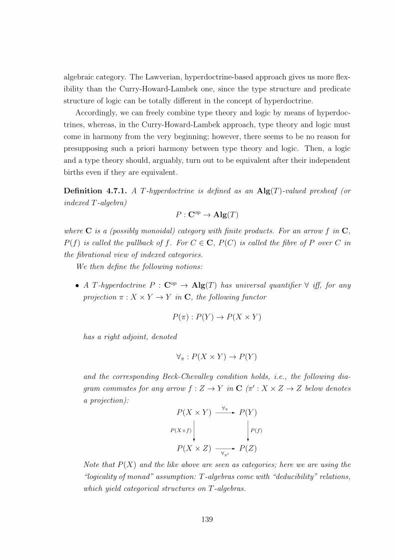
algebraic category. The Lawverian, hyperdoctrine-based approach gives us more flex-

ibility than the Curry-Howard-Lambek one, since the type structure and predicate

structure of logic can be totally different in the concept of hyperdoctrine.

Accordingly, we can freely combine type theory and logic by means of hyperdoc-

trines, whereas, in the Curry-Howard-Lambek approach, type theory and logic must

come in harmony from the very beginning; however, there seems to be no reason for

presupposing such a priori harmony between type theory and logic. Then, a logic

and a type theory should, arguably, turn out to be equivalent after their independent

births even if they are equivalent.

Definition 4.7.1. A T -hyperdoctrine is defined as an Alg(T )-valued presheaf (or

indexed T -algebra)

P : Cop → Alg(T )

where C is a (possibly monoidal) category with finite products. For an arrow f in C,

P (f) is called the pullback of f . For C ∈ C, P (C) is called the fibre of P over C in

the fibrational view of indexed categories.

We then define the following notions:

• A T -hyperdoctrine P : Cop → Alg(T ) has universal quantifier ∀ iff, for any

projection π : X × Y → Y in C, the following functor

P (π) : P (Y )→ P (X × Y )

has a right adjoint, denoted

∀π : P (X × Y )→ P (Y )

and the corresponding Beck-Chevalley condition holds, i.e., the following dia-

gram commutes for any arrow f : Z → Y in C (π′ : X × Z → Z below denotes

a projection):

P (X × Y ) P (Y )

P (X × Z) P (Z)?

P (X×f)

-∀π

?

P (f)

-∀π′

Note that P (X) and the like above are seen as categories; here we are using the

“logicality of monad” assumption: T -algebras come with “deducibility” relations,

which yield categorical structures on T -algebras.

139

• A T -hyperdoctrine P : Cop → Alg(T ) has existential quantifier ∃ iff, for any

projection π : X × Y → Y in C, P (π) : P (Y ) → P (X × Y ) has a left adjoint,

which shall be denoted as

∃π : P (X × Y )→ P (Y )

and the corresponding Beck-Chevalley diagram commutes for any f : Z → Y in

C (π′ : X × Z → Z below is a projection):

P (X × Y ) P (Y )

P (X × Z) P (Z)?

P (X×f)

-∃π

?

P (f)

-∃π′

• A T -hyperdoctrine P : Cop → Alg(T ) has equality = iff, for any diagonal

δ : X → X ×X in C, the following functor

P (δ) : P (X ×X)→ P (X)

has a left adjoint, which shall be denoted as

Eqδ : P (X)→ P (X ×X).

A quantified T -hyperdoctrine is defined as a T -hyperdoctrine having ∀ and ∃. A first-

order T -hyperdoctrine is defined as a T -hyperdoctrine having ∀, ∃, and =.

In standard, categorical developments of regular, coherent, and intuitionistic log-

ics, Frobenius Reciprocity is usually assumed as well as Beck-Chevalley conditions.

Here we do not generally assume Frobenius Reciprocity.

The main reason is that Frobenius Reciprocity is not appropriate for certain logical

systems, including quantum logic; recall that the Frobenius Reciprocity condition

for existential quantifier involves the distributivity of ∃ over ∧, a kind of infinitary

distributivity law (∃ may be seen as infinite joins), which is not generally acceptable

in quantum logic.

In sequent calculi with restricted context formulae or “visibility”, like Basic Logic

by Sambin et al., Frobenius Reciprocity is actually harmful to obtain complete se-

mantics. Note that we always assume Beck-Chevalley conditions, since it is logically

indispensable to interpret the substitution of terms for variables. Categorical models

without Beck-Chevalley properties are inadequate as semantics of logic.

140

We sometimes consider quantified hyperdoctrines without one of ∃ and ∀. For

example, (topological) geometric logic only has existential quantifier in general, and

thus it is natural to regard T -hyperdoctrines with ∃ only as being already quantified

in the case of geometric logic.

The principle of comprehension in set theory can be understood in categorical

terms of fibration as originally discovered by Lawvere and Benabou. When we talk

about comprehension, we assume that each T -algebra has a greatest element > with

respect to its deducibility ordering, and that greatest elements are preserved by ho-

momorphisms of T -algebras (the assumption that the finite power set monad is a

submonad of T is sufficient for justifying these).

T -hyperdoctrines can be seen as indexed categories, since T -algebras can be re-

garded as categories. We are therefore able to apply the Grothendieck construction

to a T -hyperdoctrine

P : Cop → Alg(T )

thus obtaining a fibred category ∫P

which can be described as follows. An object of∫P is a pair (X, a) where X is an

object of C, and a is an object of a T -algebra P (X) seen as a category. An arrow of∫P from (X, a) to (Y, b) is a pair (f, k) where f is an arrow in C from X to Y , and k

is an arrow in P (X) from a to P (f)(b) (note that, in P (X), at most one arrow exists

between two objects).

Definition 4.7.2. A T -hyperdoctrine P : Cop → Alg(T ) has comprehension - iff

the truth functor defined below

> : C→∫P

has a right adjoint, which shall be denoted as

- :

∫P → C.

The truth functor > is defined as follows. Concerning the object part, > maps an

object X ∈ C to an object

(X,>P (X)) ∈∫P

where >P (X) denotes the greatest element of a T -algebra P (X). Regarding the arrow

part, > maps an arrow f : X → Y in C to an arrow (f, !) in∫P from (X,>P (X)) to

(Y,>P (Y )) where ! is a unique arrow from >P (X) to P (f)(>P (Y )), which equals >P (X).

141

Higher-order T -hyperdoctrines are defined by requiring additional conditions for

higher type structures and truth value objects as follows.

Definition 4.7.3. A higher-order T -hyperdoctrine or a T -tripos is defined as a T -

hyperdoctrine P : Cop → Alg(T ) such that

• the base category C is Cartesian closed;

• P has quantifiers ∀, ∃, equality =, and comprehension -;

• P has an truth value object in the following sense: there exists

Ω ∈ C

such that P is naturally equivalent to

HomC(-,Ω)

where P is seen as a Set-valued functor by composition with the forgetful functor

from Alg(T ) to Set. A truth value object is also called a generic object or truth

value object.

If T represents intuitionistic logic, then higher-order T -hyperdoctrines (aka. T -

triposes) are almost equivalent to toposes (technically, there is a little bit more triposes

than toposes; for a precise account of the adjunction between them, see [98]). We may

thus consider that the concept of higher-order T -hyperdoctrine or T -tripos logically

correspond to the concept of topos relativized to a monad T .

4.8 Duality as Categorical Semantics

Let us recall the setting of duality induced by Janusian (or schizophrenic) objects

in the general style of Johnstone-Dimov-Tholen. That is, we have two categories

C and D with faithful functors U : C → Set and V : D → Set, and a Janusian

object Ω which live in both C and D. Then, two representable functors HomC(-,Ω)

and HomD(-,Ω) give us dual adjunction between C and D (under the assumption of

initial lifting properties of Ω).

Now suppose that D is Alg(T ) for a monad T as in our Space-Algebra duality,

and that C has finite products. We are thus thinking of the following dual adjunction

HomAlg(T )(-,Ω) a HomC(-,Ω) : Cop → Alg(T ).

142

Our proposal is to regard HomC(-,Ω) as a T -hyperdoctrine. We call T -hyperdoctrines

arising in this way duality T -hyperdoctrines or Stonean T -hyperdoctrines. Note that

the domain category C of a duality T -hyperdoctrine always comes with a faithful

functor U : C→ Set.

According to our logicality assumption, every T -algebra is endowed with a partial

order to represent a deductive relation. In particular, Ω is thus endowed with a partial

order ≤Ω, which canonically induce a partial order on HomC(X,Ω) for X ∈ C: i.e.,

u ≤ v for u, v ∈ HomC(X,Ω) iff for any x ∈ U(X),

U(u)(x) ≤ U(v)(x).

In the following, we assume that Ω is complete with respect to the ordering ≤Ω.

When do duality T -hyperdoctrines have logical structures such as quantifiers? The

existence of adjoints of pullbacks of projections and diagonals can be shown in quite

general situations, via the adjoint functor theorem, as in the following propositions.

At the same time, however, Beck-Chevalley conditions are just assumed in them,

and they do not provide how those adjoints actually operate. Soon after the following

three propositions, we prove more specialized propositions in which Beck-Chevalley

conditions are naturally derived, and it is quite clear how those adjoints that represent

logical constants operate.

Proposition 4.8.1. Assume that a duality T -hyperdoctrine

HomC(-,Ω) : Cop → Alg(T )

satisfies the following two conditions.

• For any X ∈ C, HomC(X,Ω) has colimits (i.e., arbitrary joins).

• The faithful functor associated with C

U : C→ Set

commutes with colimits in the following sense: for any X ∈ C and any fi ∈HomC(X,Ω) where i ∈ I, it holds that∨

i∈I

(U(fi)) = U(∨i∈I

fi)

where∨i∈I(U(fi)) is the meet of U(fi) | i ∈ I in ΩU(X), i.e., for any x ∈ X,

(∨i∈I

U(fi))(x) =∨i∈I

(U(fi)(x)).

143

Then, the duality T -hyperdoctrine HomC(-,Ω) : Cop → Alg(T ) has universal quanti-

fier ∀, if the corresponding Beck-Chevalley condition holds.

Proof. Let π : X × Y → Y be a projection in C. We have to show that HomC(π,Ω)

has a right adjoint. In order to prove this, it suffices to show that HomC(π,Ω)

preserves every colimit, i.e., join. Let fi | i ∈ I ⊂ HomC(Y,Ω). Since we have

HomC(π,Ω)(∨i∈I

fi) = (∨i∈I

fi) π

and since U is faithful, it is enough to prove the following in order to show that

HomC(π,Ω) preserves any join:

U((∨i∈I

fi) π) = U(∨i∈I

fi π).

This is shown as follows: for z ∈ U(X × Y ),

U((∨i∈I

fi) π)(y) = U(∨i∈I

fi) U(π)(z)

= (∨i∈I

U(fi)) U(π)(z)

=∨i∈I

(U(fi)(U(π)(z)))

=∨i∈I

(U(fi π)(z))

= (∨i∈I

U(fi π))(z)

= U(∨i∈I

fi π)(z).

This completes the proof.

We can prove the following in a similar way.

Proposition 4.8.2. Assume that a duality T -hyperdoctrine HomC(-,Ω) : Cop →Alg(T ) satisfies the following two conditions.

• For any X ∈ C, HomC(X,Ω) has limits (i.e., arbitrary meets).

• The faithful functor U : C→ Set commutes with limits in the following sense:

for any X ∈ C and any fi ∈ HomC(X,Ω) where i ∈ I, it holds that∧i∈I

(U(fi)) = U(∧i∈I

fi)

where∧i∈I(U(fi)) is the meet of U(fi) | i ∈ I in ΩU(X).

144

Then, the duality T -hyperdoctrine has existential quantifier ∃, if the corresponding

Beck-Chevalley condition holds.

Proposition 4.8.3. Assume that a duality T -hyperdoctrine HomC(-,Ω) : Cop →Alg(T ) satisfies the following two conditions.

• For any X ∈ C, HomC(X,Ω) has limits.

• The faithful functor U : C→ Set commutes with limits.

Then, the duality T -hyperdoctrine HomC(-,Ω) : Cop → Alg(T ) has equality =.

Proof. Let δ : X → X×X be a diagonal in C. We have to show that HomC(δ,Ω) has a

left adjoint. In order to prove this, it suffices to show that HomC(δ,Ω) preserves every

meet. Let fi | i ∈ I ⊂ HomC(X × X,Ω). Since we have HomC(δ,Ω)(∧i∈I fi) =

(∧i∈I fi)δ and since U is faithful, it is enough to prove U((

∧i∈I fi)π) = U(

∧i∈I fi

π). This is shown as follows: for x ∈ U(X),

U((∧i∈I

fi) δ)(x) = U(∧i∈I

fi) U(δ)(x)

= (∧i∈I

U(fi)) U(δ)(x)

=∧i∈I

(U(fi δ)(x))

= U(∧i∈I

fi δ)(x).

This completes the proof.

In the following proposition, we use a lifting condition analogous to the initial

lifting conditions in Johnstone-Dimov-Tholen’s dual adjunction theorem [81, 232].

Proposition 4.8.4. Consider a duality T -hyperdoctrine HomC(-,Ω) : Cop → Alg(T )

such that the associated faithful functor U : C → Set preserves products. Given a

projection π : X × Y → Y in C and v ∈ HomC(X × Y,Ω), we define

Aπv : U(Y )→ Ω

as follows: for y ∈ U(Y ),

Aπv (y) :=∧U(v)(x, y) | x ∈ U(X).

145

If “Aπv lifts to ∀π”, i.e., there is ∀π : HomC(X × Y,Ω) → HomC(Y,Ω) such that for

any v ∈ HomC(X × Y,Ω),

∀π(v) ∈ HomC(Y,Ω) and U(∀π(v)) = Aπv ,

then the duality T -hyperdoctrine HomC(-,Ω) : Cop → Alg(T ) has universal quantifier

∀.

Proof. We first show that ∀π defined above is a right adjoint of HomC(π,Ω). To show

the adjointness, suppose u ≤ ∀π(v) for u ∈ HomC(Y,Ω) and v ∈ HomC(X × Y,Ω).

Then we have

U(u)(y) ≤ U(∀π(v))(y)

for y ∈ Y . The assumptions then imply that

U(u)(y) ≤ Aπv (y) =∧U(v)(x, y) | x ∈ U(X).

Thus, for any x ∈ X,

U(u) U(π)(x, y) ≤ U(v)(x, y).

Since U is a functor, we obtain

HomC(π,Ω)(u) = u π ≤ v.

The converse can be proven in a similar way.

It remains to show the following Beck-Chevalley condition: for f : Z → Y ,

π : X × Y → Y , and π′ : X × Z → Z in C,

HomC(f,Ω) ∀π = ∀π′ HomC(X × f,Ω).

It is then sufficient to show the following: for v ∈ HomC(X × Y,Ω),

∀π(v) f = ∀π′(v (X × f)).

Since U is faithful, it is enough to show

U(∀π(v) f) = U(∀π′(v (X × f))),

which is equivalent to the following: for z ∈ Z,

U(∀π(v)) U(f)(z) = U(∀π′(v (X × f)))(z).

The assumptions imply that this is equivalent to:

Aπv (U(f)(z)) = Aπ′

v(X×f)(z).

146

This can be calculated as follows:∧x∈U(X)

U(v)(x, U(f)(z)) =∧

x∈U(X)

U(v (X × f))(x, z).

At the same time, we have:

U(v (X × f))(x, z) = U(v) U(f)(z).

We have thus shown the Beck-Chevalley condition.

The case of existential quantifier ∃ can be proven in a similar way:

Proposition 4.8.5. Consider a duality T -hyperdoctrine HomC(-,Ω) : Cop → Alg(T )

such that U : C→ Set preserves products. Given a projection π : X × Y → Y in C

and v ∈ HomC(X × Y,Ω), we define Eπv : U(Y )→ Ω as follows: for y ∈ U(Y ),

Eπv (y) :=

∨U(v)(x, y) | x ∈ U(X).

If “Eπv lifts to ∃π”, i.e., there is ∃π : HomC(X × Y,Ω) → HomC(Y,Ω) such that for

any v ∈ HomC(X × Y,Ω),

∃π(v) ∈ HomC(Y,Ω) and U(∃π(v)) = Aπv ,

then the duality T -hyperdoctrine HomC(-,Ω) : Cop → Alg(T ) has existential quanti-

fier ∃.

In the following case of equality, we explicitly use the least element of Ω.

Proposition 4.8.6. Consider a duality T -hyperdoctrine HomC(-,Ω) : Cop → Alg(T )

such that U : C → Set preserves products. Given a diagonal δ : X → X ×X in C

and v ∈ HomC(X,Ω), we define Iδv : U(X ×X)→ Ω as follows: for x, x′ ∈ U(X),

Iδv(x, x′) =

U(v)(x) if x = x′

⊥ otherwise

If there is Eqδ : HomC(X,Ω)→ HomC(X×X,Ω) such that for any v ∈ HomC(X,Ω),

Eqδ(v) ∈ HomC(Y,Ω) and U(Eqδ(v)) = Iδv ,

then the duality T -hyperdoctrine HomC(-,Ω) : Cop → Alg(T ) has equality =.

147

Proof. To show that Eqδ with the properties above is a left adjoint of HomC(δ,Ω),

we first assume that

Eqδ(v) ≤ u

where v ∈ HomC(X,Ω) and u ∈ HomC(X ×X,Ω). Then we have

U(Eqδ(v))(x, x′) ≤ U(u)(x, x′).

By letting x′ = x, it follows from the assumption U(Eqδ(v)) = Iδv that

Iδv(x, x) = U(v)(x) ≤ U(u) U(δ)(x) = U(u δ)(x).

This implies that

v ≤ u δ.

The converse can be shown in a similar way.

In the case of comprehension, we make the following additional assumption on

the lifting of restricted maps that originally come from arrows in C: for any arrow

f : Y → X in C and any A ⊂ U(X), if there is X ′ ∈ C with U(X ′) = A, then the

restriction of U(f) to A lifts to an arrow in C, i.e., there is an arrow f ′ : Y → X ′ in C

such that U(f ′) is the restriction of U(f) to A. This actually holds in most concrete

categories including the category of topological spaces and the category of algebras

of a monad on Set.

Proposition 4.8.7. Consider a duality T -hyperdoctrine HomC(-,Ω) : Cop → Alg(T ),

its fibred category∫

HomC(-,Ω) derived via the Grothendieck construction, and the

truth functor (see Definition 4.7.2)

> : C→∫

HomC(-,Ω).

If U(>Hom(X,Ω))(x) = >Ω for every X ∈ C and x ∈ U(X), and if there is a functor

Z :

∫HomC(-,Ω)→ C

such that the following hold:

• for (X, v) ∈∫

HomC(-,Ω), U(Z(X, v)) = x ∈ U(X) | U(v)(x) = >Ω;

• for an arrow (f, k) in∫

HomC(-,Ω), U(Z(f, k)) = U(f),

148

then the duality T -hyperdoctrine HomC(-,Ω) : Cop → Alg(T ) has comprehension -(the assumption intuitively means the correspondence (X, v) 7→ x ∈ X | v(x) = >Ωwith (f, k) 7→ f over Set lifts to that over C).

Proof. We show that Z is a right adjoint of the truth functor >. Let

(f, k) : >(Y )→ (X, v)

be an arrow in∫

HomC(-,Ω) where v ∈ HomC(X,Ω). Since by definition

>(Y ) = (Y,>HomC(Y,Ω)),

and since k above exists, the following must hold:

Hom(f,Ω)(v) = >HomC(X,Ω).

It follows from v f = >HomC(X,Ω) that for any x ∈ U(X),

U(v) U(f)(x) = >Ω.

Thus, the range of U(f) : U(Y ) → U(X) is actually included in U(Z(X, v)). Define

a map

f : U(Y )→ U(Z(X, v))

as the map obtained by restricting the range of U(f) into U(Z(X, v)). Then, the

assumption of the proposition tells us that there is an arrow

g : Y → Z(X, v)

such that U(g) = f . The correspondence f 7→ g gives us a natural isomorphism to

show that Z is a right adjoint of the truth functor.

All the assumptions of the propositions above are satisfied if C = Set, i.e., we

consider the dual adjunction between Set and Alg(T ), and the corresponding duality

T -hyperdoctrine HomSet(-,Ω) : Setop → Alg(T ), which turns out to be a model of

higher-order logic over T .

Theorem 4.8.8. Let C = Set in a duality T -hyperdoctrine, i.e., consider

HomSet(-,Ω) : Setop → Alg(T ),

(which is part of the Set-Alg-duality mentioned above). The Set-Alg-duality T -

hyperdoctrine is a higher-order T -hyperdoctrine.

Proof. Every duality T -hyperdoctrine has an truth value object. Set is Cartesian

closed. It thus follows from the propositions above that HomSet(-,Ω) : Setop →Alg(T ) is a higher-order T -hyperdoctrine.

149

4.9 Geometric Logic, Convexity Logic, and Quan-

tum Logic, Categorically

In this section we give sample applications of the theory above to topological geometric

logic, convex geometric logic, and categorical quantum logic, thereby illustrating what

the theory means in concrete situations. “Topological geometric logic” in our terms is

usually called just “geometric logic” (it is the logic that is invariant under geometric

morphisms of toposes). Convex geometric logic is, to our knowledge, a new concept.

Let us think of well-known dual adjunctions between topological spaces Top and

frames Frm, and in particular its predicate functor

HomTop(-,Ω) : Topop → Frm

where it should be noted that not only the two-element frame 2 but also any frame

Ω induces a dual adjunction between Top and Frm; this is a simple consequence of

general duality theory (any of duality theories [149, 195, 81] works for this purpose).

The following is an immediate consequence of the propositions above.

Corollary 4.9.1. The duality hyperdoctrine

HomTop(-,Ω) : Topop → Frm

has existential quantifier ∃. In particular, the open set hyperdoctrine HomTop(-,2) :

Topop → Frm has existential quantifier ∃. Thus, they give hyperdoctrine models of

(topological) geometric logic.

To exemplify the underlying idea of this, let us consider the simplest case of the

open set functor. It is then crucial to notice that Eπv in Proposition 4.8.5 gives us

an open set by taking the inverse image of 1 ∈ 2 under it. This is true because any

topology is closed under arbitrary unions. Since a topology is not necessarily closed

under arbitrary intersections, the predicate functors above do not necessarily have

universal quantifier. Note that (topological) geometric logic does not have universal

quantifier.

As discussed above, there are dual adjunctions between convex structures and

Scott’s continuous lattices (see Jacobs [146] and Chapter 2; the Jacobs duality for

preframes can be recasted in terms of continuous lattices). In light of those duali-

ties, we consider Scott’s continuous lattices ContLat to represent pointfree convex

structures, just as frames represent pointfree topological spaces.

150

There are two concepts of abstract convex structures, and accordingly two kinds of

dual adjunctions. Let us denote by Conv the category of convexity spaces (for details,

see van de Vel [270]), and by Alg(D) the category of algebras of the distribution

monad D, or equivalently barycentric algebras (for details, see Jacobs [146]). The

following is an immediate consequence of the propositions above.

Corollary 4.9.2. The Conv-based duality hyperdoctrine

HomConv(-,Ω) : Convop → ContLat

has universal quantifier ∀. The Alg(D)-based duality hyperdoctrine

HomAlg(D)(-,Ω) : Alg(D)op → ContLat

has universal quantifier ∀.

Thus, they give hyperdoctrine models of “convex geometric logic”, which does

not have existential quantifier, since in general the set of convex subsets is not closed

under arbitrary unions.

We can even apply the same idea to a dual adjunction between measurable spaces

and σ-complete Boolean algebras (see Chapter 2 and Chapter 5).

There are different conceptions of quantum logic and its algebras. The lattice of

projection operators on a Hilbert space is a standard algebra of quantum logic. We can

think of different categories encompassing those standard algebras of quantum logic,

including the category of orthomodular lattices, denoted OML and the category

of effect algebras, denoted EA. The latter is more general than the former, and

encompasses the algebras of so-called effects of a Hilbert space as well as the algebra

of projection operators.

Both OML and EA are algebraic categories, i.e., can be described as categories of

algebras of monads on Set. Effect algebras only have negation and partial disjunction,

and thus they are logically less expressive than orthomodular lattices. In this section,

we mainly work with OML, and variants of it.

Fix a Hilbert space H, and let P(H) denote the lattice of projection operators on

H. We can see P(H) as a set and as an algebra, and hence we have a dual adjunction

between Set and OML induced by P(H) (HomSet(X,P(H)) is obviously closed under

the pointwise operations induced from the operations of P(H); this amounts to the

harmony condition). Let us look at the logic of the adjunction, i.e., see

HomSet(-,P(H)) : Setop → OML

151

as a Q-hyperdoctrine where Q is the monad corresponding to OML. For the brevity

of description, we drop the subscript “Set” of “HomSet(-,P(H))”.

Lemma 4.9.3. Hom(-,P(H)) has quantifiers ∀ and ∃.

Proof. Let π : X × Y → Y be a projection in Set. We define

∀π : Hom(X × Y,P(H))→ Hom(Y,P(H));

∀π : Hom(X × Y,P(H))→ Hom(Y,P(H))

as follows: given v ∈ Hom(X × Y,P(H)) and y ∈ Y , let

∀π(v)(y) :=∧v(x, y) | x ∈ X;

∃π(v)(y) :=∨v(x, y) | x ∈ X.

We claim that ∀π and ∃π are right and left adjoints of Hom(π,P(H)) respectively. To

show the case of ∀π, assume

Hom(π,P(H))(u) ≤ v

where u ∈ Hom(Y,P(H)) and v ∈ Hom(X × Y,P(H)). For (x, y) ∈ X × Y , we then

have

Hom(π,P(H))(u)(x, y) = u(y) ≤ v(x, y)

and therefore it follows that

u(y) ≤∧v(x, y) | x ∈ X = ∀π(v)(y).

We have thus shown that

if Hom(π,P(H))(u) ≤ v, then u(y) ≤ ∀π(v)(y).

The converse can be shown by reversing the reasoning above, and so ∀π is a right

adjoint of Hom(π,P(H)). In a similar way, we can prove that ∃π is a left adjoint of

Hom(π,P(H)).

Lemma 4.9.4. Hom(-,P(H)) has equality =.

Proof. Fix a diagonal δ : X → X ×X in Set. We define

Eqδ : Hom(X,P(H))→ Hom(X ×X,P(H))

152

as follows: for v ∈ Hom(X,P(H)) and x, x′ ∈ X,

Eqδ(v)(x, x′) =

v(x) if x = x′

⊥ otherwise

where ⊥ denote the least element of P(H). In the following, we show that Eqδ is a

left adjoint of Hom(δ,P(H)). Let u ∈ Hom(X ×X,P(H)), and v ∈ Hom(X,P(H)).

Assume

Eqδ(v) ≤ u.

We want to show that

v ≤ Hom(δ,P(H))(u),

which is equivalent to the following: v ≤ u δ, i.e., v(x) ≤ u(x, x) for all x ∈ X. It

then follows from the assumption that

v(x) = Eqδ(v)(x, x) ≤ u(x, x).

The converse can be shown in a similar way.

Lemma 4.9.5. Hom(-,P(H)) has “co-equality”, i.e., there is a right adjoint of Hom(δ,P(H))

for any diagonal δ : X → X ×X in Set.

Proof. We define

CEδ : Hom(X,P(H))→ Hom(X ×X,P(H))

as follows: for v ∈ Hom(X,P(H)) and x, x′ ∈ X,

CEδ(v)(x, x′) =

P if v(x) = v(x′) = P

⊥ otherwise

where > and ⊥ denote the greatest and least elements of P(H). In the following, we

show that CEδ is a right adjoint of Hom(δ,P(H)). Let v ∈ Hom(X ×X,P(H)), and

u ∈ Hom(X,P(H)). Assume

Hom(δ,P(H))(v) ≤ u.

For x ∈ X, we then have

v δ(x) = v(x, x) ≤ u(x).

Consider CEδ(u). If v(x, x) = P , then the inequality above tells us

P ≤ u(x) = CEδ(u)(x, x).

153

Thus we have proven v ≤ CEδ(u) assuming Hom(δ,P(H))(v) ≤ u. To show the

converse, suppose v ≤ CEδ(u). This implies that

Hom(δ,P(H))(v)(x) = v(x, x) ≤ CEδ(u)(x, x) = u(x).

This completes the proof.

Lemma 4.9.6. Hom(-,P(H)) has comprehension -.

Proof. Consider the truth functor (see Definition 4.7.2)

> : Set→∫

Hom(-,P(H)).

We have to construct a right adjoint of this. Define the comprehension functor

- :

∫Hom(-,P(H))→ Set

as follows. Given (X, v) ∈∫

Hom(-,P(H)), which meansX ∈ Set and v ∈ Hom(X,P(H)),

let

(X, v) := x ∈ X | v(x) = >P(H)

where >P(H) is the greatest element of P(H). The arrow part of - is defined by

taking the first projection, i.e., (f, k) is mapped to f . To show that this gives us a

right adjoint, consider an arrow

(f, k) : >(Y )→ (X, v)

in∫

Hom(-,P(H)) where v ∈ Hom(X,P(H)). Since by definition

>(Y ) = (Y,>Hom(Y,P(H)),

the following must hold because of the existence of k:

Hom(f,P(H))(v) = >Hom(X,P(H).

This implies that the range of f : Y → X is actually included in (X, v). Define a

map

f : Y → (X, v)

as the map obtained by restricting the range of f into (X, v). The mapping f 7→f gives us the natural isomorphism required for the adjunction between the truth

functor and the comprehension functor.

154

The following proposition tells us the projection-operator-based duality hyperdoc-

trine Hom(-,P(H)) forms a model of higher-order quantum logic.

Proposition 4.9.7. Hom(-,P(H)) is a higher-order Q-hyperdoctrine or a Q-tripos.

Proof. It is obvious that P(H) is an truth value object for the Q-hyperdoctrine

Hom(-,P(H)). The base category Set is Cartesian closed. These together with the

lemmata above tell us that Hom(-,P(H)) is a higher-order Q-hyperdoctrine.

Given a frame Ω, the set-based duality hyperdoctrine Hom(-,Ω) : Setop → Frm

yields via the tripos-to-topos construction the Higgs topos of Ω-valued sets, or equiv-

alently the sheaf topos on Ω, or equivalently the topos of sets in the Ω-valued model

of set theory (aka. Heyting-valued models; see, e.g., Bell [27]).

Let us think of a quantum analogue of this. The tripos-to-topos construction

in the present context can be defined in the same way as above, that is, as the

category T(Hom(-,P(H))) of partial equivalence relations in the internal logic of a

given Hom(-,P(H)). Note that we only need deductive relations (i.e., partial orders

on fibres), conjunction, and existential quantifier when defining the tripos-to-topos

construction; they indeed exist in Hom(-,P(H)).

Now our question is how T(Hom(-,P(H))) compares to the known concept of

Takeuti-Ozawa’s quantum set theory, to be precise the P(H)-valued model of set

theory, which is defined as follows: for each ordinal α, define via the transfinite

recursrion Vα = u | u : D → P(H) and D ⊂⋃β≤α Vβ and then let V =

⋃α∈Ord Vα

where Ord is the class of all ordinals. We denote by SetP(H) the category of sets in

this model of set theory. We then have the following proposition.

Proposition 4.9.8. T(Hom(-,P(H))) embeds into SetP(H).

We finally address the issue of completeness with respect to proof-theoretic calcu-

lus, which has so far been lacking in categorical quantum logic with quantifiers (one

without quantifiers has already been developed).

Let QL denote the category of algebras of Faggian-Sambin’s propositional quan-

tum logic FS; algebraisation of logic is automatic via the well-known methods of

Abstract Algebraic Logic. For syntactic details, we refer to Faggian-Sambin [90]. FS

can be quantified in the same way as Sambin’s Basic Logic. The quantified FS can

then be typed in the same manner as typed intuitionistic logic in Pitts [229], i.e.,

just as having done above. We denote by TFSq the resulting typed quantum sequent

calculus. Using the same method as in the above proof of categorical completeness

for TFLq, we can show that the class of all QL-hyperdoctrines P : Cop → QL gives

155

sound and complete semantics for TFSq. We can refine this completeness theorem

into the following by focusing upon set-based duality hyperdoctrines above: The class

of all set-based duality QL-hyperdoctrines Hom(-,Ω) : Setop → QL where Ω ∈ QL

gives sound and complete semantics for TFSq.

We may even replace the cartesian type theory of the logic by the monoidal one, in

the same way as Ambler [15] considers logic over monoidal type theory. This is a merit

of the hyperdoctrine approach, in which logic and type theory are separated, and can

be chosen independently of each other. That is, we choose Faggian-Sambin’s quan-

tum calculus for the logic part, and Ambler’s linear type theory for the type theory

part, which amounts to SMCC (symmetric monoidal closed categories). Accordingly,

the base category of a hyperdoctrine is taken to be an SMCC with finite products;

note that we still keep cartesian products for the purpose of defining quantifiers.

Let LFSq denote the linearly typed quantum sequent calculus. The class of all QL-

hyperdoctrines P : Cop → QL over SMCC C with products gives sound and complete

semantics for LFSq. In the Hilbert hyperdoctrine KSub : Hilbop → QL, tensor ⊗maps two projections P ∈ KSub(X) and Q ∈ KSub(Y ) into P ⊗Q ∈ KSub(X ⊗ Y ),

i.e., it functions as translation between different fibres. We could then argue that

dagger-SMCC-based quantum-logic-valued hyperdoctrines enriched with a structure

to express this tensor translation between fibres give a synthesis of Birkhoff-von Neu-

mann’s quantum logic and Abramsky-Coecke’s categorical quantum mechanics.

This approach to the unification of Birkhoff-von Neumann’s quantum logic and

Abramsky-Coecke’s categorical quantum mechanics via categorical universal logic

shall be elaborated in subsequent papers.

4.10 Lawvere-Tierney Topology as Logical Trans-

lation

Given a topos E with a subobject classifier Ω, a Lawvere-Tierney topology on Ω is

equivalent to a natural transformation

j : SubE(-)→ SubE(-)

such that jC is a left-exact monad on SubC(C) for every C ∈ C. Having this corre-

spondence in mind, we define the concept of Lawvere-Tierney topology in the context

of Categorical Universal Logic as follows.

156

Definition 4.10.1. For a T -hyperdoctrine P : Cop → Alg(T ), a Lawvere-Tierney

topology on P is a natural transformation

j : P → P

such that jC : P (C) → P (C) is a left-exact monad on P (C) for each C ∈ C. We

also call a Lawvere-Tierney topology a Lawvere-Tierney operator.

Dually, a Lawvere-Tierney cotopology (or co-operator) for P is a natural trans-

formation j : P → P such that jC : P (C)→ P (C) is a right-exact comonad on P (C)

for each C ∈ C.

From a logical point of view, naturality above means that a propositional operator

j commutes with substituition of terms for variables. This is precisely true in the

syntactic (or classifying) HA-hyperdoctrine

P : Cop → HA

obtained from intuitionistic logic with quantifiers. Roughly speaking, an object of

C is a collection of typed variables, and an arrow of C is a term. Then, P maps a

collection of variables x1, ..., xn to the Heyting algebra of formulas ϕ(x1, ..., xn) with

those variables, and P (t) is the substitution of t for relevant variables. (for details,

see).

An important example of Lawvere-Tierney topology on the syntactic HA-hyperdoctrine

P is the double negation topology d : P → P defined by

dC(ϕ) = ¬¬ϕ

where C ∈ C and ϕ ∈ P (C). Note that dC : P (C) → P (C) is a closure operator on

P (C), and d is indeed a natural transformation, since substitution commutes with

double negation:

(¬¬ϕ)[t/x] = ¬¬(ϕ[t/x]).

The double negation topology induces another functor

Pd : Cop → BA

defined as follows. For C ∈ C, let

Pd(C) := ¬¬ϕ | ϕ ∈ P (C)

157

which is the Boolean algebra of those ϕ ∈ P (C) that validate double negation elimi-

nation. For an arrow t : D → C in C, which is a term, let

Pd(t) : Pd(C)→ Pd(D)

be the restriction of P (t) to Pd(C), which is possible because substitution commutes

with double negation. Then we have the following proposition stating that the double

negation topology d transforms a quantified HA-hyperdoctrine P into a quantified

BA-hyperdoctrine Pd.

Proposition 4.10.2. The hyperdoctrine Pd : Cop → BA defined above forms a quan-

tified BA-hyperdoctrine. In other words, the mapping P 7→ Pd preserves quantified

hyperdoctrine structures.

These give a categorical understanding of Godel-Gentzen’s translation from clas-

sical logic to intuitionistic logic. In the following, we abstract such such phenomena

from the viewpoint of Categorical Universal Logic, finally leading to Universal Trans-

lation Theorem below. The proposition above shall be derived as a corollary of

Universal Translation Theorem.

In addition to Godel-Gentzen’s translation, Universal Translation Theorem en-

compasses Godel-McKinsey-Tarski’s translation from intuitionistic logic to S4 modal

logic, Baaz’ translation from Lukasiewicz logic to classical logic, and Girard’s trans-

lation from intuitionistic logic to linear logic.

Definition 4.10.3. A Lawvere-Tierney topology j : P → P on a T -hyperdoctrine

P : Cop → Alg(T ) is called idempotent iff jC : P (C) → P (C) is an idempotent

monad for every C ∈ C, i.e.,

jC jC = jC .

In the following we fix a T -hyperdoctrine P : Cop → Alg(T ) and an idempotent

Lawvere-Tierney topology j on P . Note that double negation is idempotent in intu-

itionistic logic; S4 modality is idempotent; Baaz’ delta operator is idempotent; and

Girard’s exponentials are idempotent. Thus, idempotency is a natural assumption to

treat a Lawvere-Tierney topology as logical translation of such type.

Definition 4.10.4. A Lawvere-Tierney topology j : P → P on a T -hyperdoctrine

P : Cop → Alg(T ) is said to induce algebras of a monad S on Set iff the image of

jC : P (C)→ P (C) forms an algebra of S for each C ∈ C.

158

For example, the double negation topology induces Boolean algebras.

In the following, in order to capture the situation of logical translation which we

focus on, we assume that a Lawvere-Tierney topology j : P → P induces S-algebras

for some monad S.

Then, we define an Alg(S)-valued presheaf

Pj : Cop → Alg(S)

as follows. For an object C in C, let

Pj(C) = Fix(jC)

which denotes the fixpoints of jC : P (C) → P (C), i.e., jC(ϕ) | ϕ ∈ P (C). For an

arrow f : D → C in C, let

Pj(f) : Pj(C)→ Pj(D)

be the restriction of P (f) : P (C) → P (D) to Pj(C), which is possible, since the

naturality of j gives us

jD P (f) = P (f) jC ,

which implies that the image of Pj(f) is included in Pj(D); hence the consistency of

the definition of Pj(f).

Theorem 4.10.5. We first assume that

jD(∀π(jC×D(ϕ))) ≤ ∀π(jC×D(ϕ))

for a projection π : C×D → D in C, ϕ ∈ Pj(C×D), and ψ ∈ Pj(D). If the original

T -hyperdoctrine

P : Cop → Alg(T )

is a first-order T -hyperdoctrine, then the following S-hyperdoctrine induced by a Lawvere-

Tierney topology j on P

Pj : Cop → Alg(S)

is a first-order S-hyperdoctrine as well.

Proof. We first show the existence of universal quantifier. Assume that

Pj(π)(ψ) ≤ ϕ

159

for a projection π : C × D → D in C, ϕ ∈ Pj(C × D), and ψ ∈ Pj(D). Let

∀π : P (C×D)→ P (D) denote the universal quantifier of P with respect to π. Define

∀jπ : Pj(C ×D)→ Pj(D)

by

∀jπ(ξ) = jD(∀π(ξ))

where ξ ∈ Pj(C ×D). Note that ∀jπ(ξ) ∈ Pj(D). Now we have

Pj(π)(ψ) = P (π)(ψ) ≤ ϕ,

since ψ ∈ Pj(D). This implies that ψ ≤ ∀π(ϕ). Since jD is a monad, it follows from

∀π(ϕ) ≤ jD(∀π(ϕ)) that

ψ ≤ jD(∀π(ϕ)) = ∀jπ(ϕ).

To show the converse, assume ψ ≤ ∀jπ(ϕ). Since ϕ is a fixpoint of jC×D, we have

jC×D(ϕ) = ϕ. Then, it holds that

ψ ≤ jD(∀π(jC×D(ϕ))).

It then follows from the assumption jD(∀π(jC×D(ϕ))) ≤ ∀π(jC×D(ϕ)) that

ψ ≤ ∀π(jC×D(ϕ)) = ∀π(ϕ).

Since ∀π is a right adjoint of P (π), we have P (π)(ψ) ≤ ϕ. It then follows from

ψ ∈ Pj(D) that Pj(π)(ψ) ≤ ϕ. Thus, ∀jπ is a right djoint of Pj(π).

We next show the existence of existential quantifier.

We finally show the existence of equality. For a diagonal δ : C → C ×C in C, let

Eqδ denote the equality of P with respect to δ. Then, define

Eqjδ : Pj(C × C)→ Pj(C)

by

Eqjδ(ξ) = jC(Eqδ(ξ))

where ξ ∈ Pj(C × C). Note that Eqjδ(ξ) ∈ Pj(C). In order to prove that this gives a

left adjoint of Pj(δ), we first assume that

Eqjδ(ϕ) ≤ ψ

for ϕ ∈ Pj(C × C) and ψ ∈ Pj(C). Since jC is a monad, we have

Eqδ(ϕ) ≤ jC(Eqδ(ϕ)) ≤ ψ.

160

Since Eqδ is a left adjoint of P (δ), it holds that ϕ ≤ P (δ)(ψ). But we have ψ ∈ Pj(C),

and thus

ϕ ≤ Pj(δ)(ψ).

To prove the converse, assume ϕ ≤ Pj(δ)(ψ). Then, we have Eqδ(ϕ) ≤ ψ. Since jC is

a monad, it follows that

Eqjδ(ϕ) = jC(Eqδ(ϕ)) ≤ jC(ψ) = ψ.

Thus, Eqjδ is a left adjoint of P (δ).

The higher-order version of this universal translation theorem is left for future

work; the particular case of FL triposes is shown above.

4.11 Remarks on Duality in Logic and Algebraic

Geometry

Categorical logic, in particular topos theory, has shown substantial analogies between

(geometric) logic and algebraic geometry. In this section let us see duality-theoretical

analogies between logic and algebraic geometry, as briefly mentioned in Section ??.

The origin of duality, presumably, is in algebraic geometry, which in turn origi-

nates in Descartes’ analytic geometry. It is concerned with the relationships between

polynomials and their zeros (affine varieties). In logical terms, they are formulas and

their models, respectively. A symptom of duality is this: the more polynomials, the

less zeros. Elaborating this relationship, we lead to Hilbert’s Nullstellensatz, which

shall be detailed below.

Both completeness and Hilbert’s Nullstellensatz may be seen as order-theoretical

dualities, and completeness and Nullstellensatz are actually equivalent, up to a certain

point. Logical completeness can be reformulated as follows:

Form Mod(T ) = T.

Form(M) is defined as the collection of formulae valid in any M ∈ M where M is

a collection of models. We thus have:

Form Mod(T ) = the formulae valid in any model of T.

On the other hand, Hilbert Nullstellensatz states:

I V (J) =√J

161

for an ideal J ⊂ k[x1, ..., xn] with k an algebraically closed field. Recall that V (J)

gives the collection of zeros of polynomials in an ideal J , and that I(V ) gives the

collection of polynomials vanishing on V . Note that√J := p | ∃n ∈ N pn ∈ J, and

that J is called a radical ideal iff√J = J . The analogy between completeness and

Nullstellensatz would be obvious in this formulation. Why, however, is there no√

in

logic? It is because contraction holds; in the present formulation, contraction means

that if ϕ ∧ ϕ is refutable, then ϕ refutable as well. In the following formulation, the

analogy would be even more transparent:

• Completeness: T = the formulas valid on Mod(T ).

• Nullstellensatz: J = the polynomials vanishing on V (J) where J is a radical

ideal (this always holds in a Boolean ring).

Theories correspond to ideals, and models to zeros.

Completeness tells us order-theoretic duality between theories and models. We

have:

T ⊂ T ′ iff Mod(T ) ⊃Mod(T ′).

The same holds for Form. It then holds that Form and Mod give a pair of (dually)

adjoint functors (or Galois connection). Adding non-inclusion arrows and equipping

Mod(T ) with a topology, this poset-level duality is upgraded into Stone duality. In

this sense, Stone duality is a sophisticated form of completeness where there are arrows

other than inclusions, and Mod(T ) is equipped with a topology (note that Stone

topology preceded Zariski topology as noted in Bourbaki’s history of mathematids).

Nullstellensatz, on the other hand, tells us order-theoretic duality between the

radical ideals of k[x1, ..., xn] and the affine varieties over k. By adding more ar-

rows and equipping varieties with Zariski topologies, it becomes categorical equiva-

lence between finitely generated reduced k-algebras and affine varieties over k. Note

that ideals correspond to polynomial rings quotiented by them, and the “radical”

condition on ideals to the “reduced” condition on algebras. This even extends to

the scheme-theoretical duality between commutative algebras and affine schemes, in

which, however, dual structures are explicitly algebraic because schemes are equipped

with sheaves of algebras. Instead, the scheme-theoretical approach to duality works

beyond commutative structures.

The correspondence looks clear, and yet there are actually some complications

involved. There is indeed a dimensional difference: models are in Ωκ for a cardinal

κ (where Ω is a set of truth values), and varieties are in kn for a natural number n.

162

Another thing is that we think of F2 in classical logic and yet we have to think of

its algebraic closure F2 in the corresponding algebraic geometry. We can nonetheless

go beyond these complications, and establish the correspondence between complete-

ness and Nullstellensatz, and between Stone duality and Hilbert duality, both up to

GF(pn).

We can, for example, prove that completeness follows from Nullstellensatz, in the

following manner. Assume

v(ϕ(x1, ..., xn)) = 0

for any 0, 1-valuation v. We can naturally consider

ϕ ∈ F2[x1, ..., xn]

by rewriting ϕ using 0, 1, XOR (addition) and AND (multiplication) only. Then,

ϕ ∈ I (Fn2 ) = I V (J)

where

J := 〈x21 − x1, ..., x

2n − xn〉.

Nullstellensatz over F2 tells us:

I V (J) =√J.

Hence, ϕ = 0 in F2[x1, ..., xn]/√J. This implies that ¬ϕ is provable in any standard

calculus for classical logic. Note that

F2[x1, ..., xn]/√J

can be seen as a calculus and be shown to be equivalent, with respect to provability,

to LK, NK, and so fourth. Completeness thus follows from Nullstellensatz over F2.

Conversely, Nullstellensatz follows from completeness. For example, consider two

infinitary geometries over F2. One is induced by infinite coordinates (x1, x2, ..., xn, ...).

The other is induced by infinitary multiplication. A Nullstellensatz-type theorem in

the former follows from the (strong) completeness of classical propositional logic. A

Nullstellensatz-type theorem in the latter follows from the completeness of infinitary

logic (with respect to infinitary calculus). We need to assume that J in each Null-

stellensatz contains x2i −xi. Note that Nullstellensatz can fail in some∞-dimensional

geometries. Exploiting the dimensional difference, therefore, logic could contribute

to ∞-dimensional algebraic geometry.

The Hilbert-Stone correspondence allows us to go back and fourth between logic

and algebraic geometry, thus allowing for further interactions between the two fields.

For example, we have the following correspondence:

163

• A variety is irreducible iff its coordinate ring is an integral domain. This is

known in geometry, and the logic counterpart is the following: For a theory T ,

Mod(T ) is irreducible iff T is complete.

• A variety has a unique, minimal, irreducible decomposition. This one is known

in geometry as well, and the logic counterpart is the following: If T contains

finitely many atomic propositions, Mod(T ) has a unique, minimal, irreducible

decomposition.

• Compactness in logic states that X ⊂ Fml is satisfiable iff so is any finite

subset of it (Fml denotes the set of formulae). The geometric counterpart is

the following: X ⊂ F2[x1, ..., xn, ...] has a common zero iff so is any finite subset.

Note that this is not trivial, since the ring is not Noetherian.

In general, geometry over a ring R amounts to R-valued logic. The Hilbert-Stone

correspondence, however, seemingly does not hold beyond GF(pn).

164

Chapter 5

Duality and Quantum Physics

Duality meets symmetry in the present chapter, technically through the theory of

Chu spaces and the theory of coalgebras. We first develop a duality theory on the

basis of Chu space theory enriched with the logical concept of closure conditions;

whereas our first duality theory via categorical topology and algebra may be viewed

as a sort of vast extension of the duality between spatial frames and sober space, the

duality theory in this chapter can be seen as extending the duality between coatomistic

frames and T1 spaces, in which the notion of frame morphism must be changed so as

to preserve maximal filters via the inverse image operation. The duality of operational

quantum mechanics is of the same form, and may thus be classified as T1-type (as

opposed to sober-type). Note that algebraic varieties with Zarisiki topologies are

not sober but T1. The duality theory thus established allows us to improve upon

Abramsky’s representation of quantum systems and their symmetries, thus showing

that the quantum symmetry groupoid embeds into a “purely coalgebraic” category

(rather than a “fibred coalgebraic” category). Duality is, so to say, an underpinning of

symmetry. The central tenet of the present chapter is that the quantum symmetries

are the maps preserving the dynamics of measurements according to the Born rule.

5.1 Introduction to the Chapter

It is not uncommon these days to hear of applications of (the methods of) theoretical

computer science to foundations of quantum physics; broadly speaking, theoretical

computer science seems to be taking steps towards a new kind of “pluralistic unified

science” (not monistic one in logical positivism) via the language and methodology of

category theory. Among them, Abramsky [5, 7] represents quantum systems as Chu

spaces and as coalgebras, giving striking characterisations of quantum symmetries

166

based upon the classic Wigner Theorem. Revisiting his work, in the present chap-

ter, we develop a Chu-space-based theory of dualities encompassing a form of state-

observable duality in quantum physics, and thereafter improve upon his coalgebraic

characterisation of quantum symmetries from our duality-theoretical perspective, in

order to exhibit the meaning of duality.

In Pratt’s Stone Gamut paper [236], he analyses Stone-type dualities in the lan-

guage of Chu spaces, saying boldly, but with good reasons, “the notoriously difficult

notion of Stone duality reduces simply to matrix transposition.” The concept of Chu

spaces has played significant roles in fairly broad contexts, including concurrency and

semantics of linear logic; similar concepts have been used in even more diverse dis-

ciplines, like Barwise-Seligman’s classifications, Sambin’s formal topology and basic

pairs, Scott’s information systems, and state-property systems in quantum founda-

tions. This work is inspired by Pratt’s perspective on Chu spaces, extending the

realm of duality theory built upon the language of Chu spaces by enriching it with a

generic concept of closure conditions.

In general, we have two types of dualities, namely sober-type and T1-type ones,

between set-theoretical concepts of space and their point-free, algebraic abstractions,

which shall be called point-set spaces and point-free spaces respectively. The differ-

ence between the two types of dualities in fact lies in the difference between maximal

and primal spectra. Our duality theory in this chapter focuses upon T1-type dualities

between point-set and point-free spaces. The logical concept of closure conditions is

contrived to the end of treating different sorts of point-set and point-free spaces in a

unified manner, allowing us to discuss at once topological spaces, measurable spaces,

closure spaces, convexity spaces, and so fourth. In a nutshell, the concept of closure

conditions prescribes the notion of space. Whilst a typical example of sober-type du-

ality is the well-known duality between sober spaces and spatial frames, an example

of T1-type duality is a duality between T1 closure spaces and atomistic meet-complete

lattices, including as particular instances state-observable dualities between quantum

state spaces (with double negation closures) and projection operator lattices in the

style of operational quantum mechanics (see Coecke and Moore [66] or Moore [208]).

Our theory of T1-type dualities enables us to derive a number of concrete T1-

type dualities in various contexts, which include T1-type dualities between Scott’s

continuous lattices and convexity spaces, between σ-complete boolean algebras and

measurable spaces, and between topological spaces and frames, to name but a few.

Let us illustrate by a topological example a striking difference between sober-type

and T1-type dualities. The T1-type duality in topology is a duality between T1

167

spaces and coatomistic frames in which continuous maps correspond not to frame

homomorphisms but to maximal homomorphisms, which are frame homomorphisms

f : L→ L′ such that, given a maximal join-complete ideal M ⊂ L′, f−1(M) is again

a maximal join-complete ideal. Although the duality for T1 spaces is not mentioned

in standard references such as Johnstone [149], nevertheless, we consider it important

for the reason that some spaces of interest are not sober but T1: e.g., affine varieties

in kn with k an ACF (i.e., algebraically closed field) are non-sober T1 spaces (if they

are not singletons). Note that Bonsangue et al. [41] shows a duality for T1 spaces

via what they call observation frames, which are frames with additional structures,

yet the T1-type duality above only relies upon plain frame structures.

Whilst sober-type dualities are based upon prime spectrum “Spec”, T1-type du-

alities are based upon maximal spectrum “Spm”. Different choices of spectrum lead

to different Chu representations of algebras A concerned: maximal spectrum gives

(A, Spec(A), e) and prime spectrum gives (A, Spm(A), e) where e is two-valued and

defined in both cases by: e(a,M) = 1 iff a ∈ M . Accordingly, the correspond-

ing classes of Chu morphisms are distinctively different: e.g., in locale theory, the

Spec-based representation characterises frame homomorphisms as Chu morphisms

(as shown in Pratt [236]), and the Spm-based representation characterises maximal

homomorphisms as Chu morphisms (as shown in this chapter for general point-free

spaces encompassing frames as just a particular instance). In this way, the Chu space

formalism yields a natural account of why different concepts of homomorphisms ap-

pear in sober-type and T1-type dualities.

As in the case above, Chu morphisms can capture different sorts of homomor-

phisms by choosing different Chu representations. This is true even in quantum

contexts, and in particular we can represent quantum symmetries as Chu morphisms

by a suitable Chu representation. Coalgebras are Chu spaces with dynamics, and

we have a coalgebraic representation of quantum symmetries as well. To be precise,

in moving from Chu space to coalgebras, Abramsky [7] relies upon a fibred cate-

gory∫

F obtained by gluing categories Coalg(FQ)’s for every Q ∈ Set where FQ

is an endofunctor on Set. He uses the Grothendieck construction to “accommodate

contravariance” within a coalgebraic framework, fully embedding the groupoid of

symmetries into the fibred category∫

F.

Looking at the∫

F representation from a duality-theoretical perspective, we con-

sider it odd that there is no structural relationship taken into account between quan-

tum state spaces and projection operator lattices: both are seen as mere sets. For the

very reason, Q (which is a projection lattice in a quantum context) first have to be

168

fixed in the endofunctor FQ on Set (objects of which are state spaces in a quantum

context), and thereafter Coalg(FQ)’s are glued together to accommodate contravari-

ance regarding Q ∈ Set. This two-step construction is reduced in the present chapter

into a simpler, one-step one as follows.

First of all, there is actually a dual, structural relationship between quantum state

spaces and projection lattices with the latter re-emerging as the fixpoints (or algebras)

of double negation closures (or monads) on the former. This means that Q above

can be derived, rather than independently assumed, from a closure structure, if one

works on the base category of closure spaces, rather than mere sets. The closure-

based reformulation of the∫

F representation leads us to a “Born” endofunctor B

on closure spaces, and to its coalgebra category Coalg(B), which turns out to be

strictly smaller than fairly huge∫

F, but still large enough to represent the quantum

symmetry groupoid, thus yielding a purely coalgebraic representation and enabling to

accommodate contravariance within the single coalgebra category Coalg(B) rather

than the fibred∫

F glueing different Coalg(FQ)’s for all sets Q; notice that con-

travariance is incorporated into the dualisation process of taking the fixpoints (or

algebras) of closures.

5.2 Duality and Chu Space Representation

We first review basic concepts and notations on Chu spaces and closure spaces.

Chu Spaces Let us fix a set Ω. A Chu space over Ω is a triple (S,A, e) where S

and A are sets, and e is a map from S × A to Ω. Ω is called the value set, and e

the evaluation map. A Chu morphism from (S,A, e) to (S ′, A′, e′) is a tuple (f ∗, f∗)

of two maps f ∗ : S → S ′ and f∗ : A′ → A such that e(x, f∗(a′)) = e′(f ∗(x), a′). The

category of Chu spaces and Chu morphisms is self-dual, and forms a ∗-autonomous

category, giving a fully complete model of linear logic.

For a Chu space (S,A, e : S × A → Ω) and a ∈ A, e(-, a) : S → Ω is called a

column of (S,A, e). We denote the set of all columns of (S,A, e) by Col(S,A, e). On

the other hand, e(x, -) : A → Ω is called a row of (S,A, e). We denote the set of

all rows of (S,A, e) by Row(S,A, e). If Ω is ordered, then we equip Col(S,A, e) and

Row(S,A, e) with the pointwise orderings: e.g., in the case of Col(S,A, e), this means

that, for a, b ∈ A,

e(-, a) ≤ e(-, b) iff e(x, a) ≤ e(x, b) for any x ∈ S.

169

A Chu space (S,A, e) is called extensional iff all the columns are mutually different,

i.e., if e(x, a) = e(x, b) for any x ∈ S then a = b. On the other hand, a Chu space

(S,A, e) is called separated iff all the rows are mutually different, i.e., if e(x, a) =

e(y, a) for any a ∈ A then x = y.

Closure Spaces Closure spaces may be seen as either a set with a closure operator

or a set with a family of subsets that is closed under arbitrary intersections. We

denote by C(S) the set of closed subsets of a closure space S, and by cl(-) the closure

operator of S. In this chapter we always assume ∅ ∈ C(S) or equivalently cl(∅) = ∅.Note then that there is a unique closure structure on a singleton. A map f : S → S ′ is

called closure-preserving iff f−1(C) ∈ C(S) for any C ∈ C(S ′) iff f(cl(A)) ⊂ cl(f(A)).

We denote by Clos the category of closure spaces and closure-preserving maps, which

has products and coproducts. A closure space is called T1 iff any singleton is closed.

5.2.1 Chu Representation of Quantum Systems

Abramsky [7] represents a quantum system as a Chu space defined via the Born rule,

which provides the predictive content of quantum mechanics. Given a Hilbert space

H, he constructs the following Chu space over the unit interval [0, 1]:

(P(H),L(H), eH : P(H)× L(H)→ [0, 1])

where P(H) denotes the set of quantum states as rays (i.e., one-dimesional subspaces)

in H, L(H) denotes the the set of projection operators (or projectors) on H, and

finally the evaluation map eH is defined as follows (let [ϕ] = αϕ | α ∈ C):

eH([ϕ], P ) =〈ϕ|Pϕ〉〈ϕ|ϕ〉

.

We consider that Chu spaces have built-in dualities, or they are dualities without

structures: whilst S and A have no structure, e still specifies duality. The category

of Chu spaces has duals in terms of monoidal categories; this is internal duality. Can

we externalise internal duality in Chu spaces by restoring structures on S and A

through e? It is an inverse problem as it were. In the quantum context, it amounts

to explicating the structures of P(H) and L(H) that give (external) duality.

The first observation is the bijective correspondences:

P(H) ' e(ϕ, -) | ϕ ∈ P(H) ' c ∈ Col(P(H),L(H), eH) | the precisely one 1 appears in c.

170

So, the states are the atoms of L(H): in this way we can recover P(H) from L(H).

This means L(H) should be equipped with the lattice structure as in Birkhoff-von-

Neumann’s quantum logic. Although we have L(H) ' e(-, P ) | P ∈ L(H), it is

not clear at this stage what intrinsic structure of P(H) enables to recover L(H) from

P(H). Let us see that a double negation operator on P(H) does the job.

Define (-)⊥ : P(P(H))→ P(P(H)) as follows: for X ⊂ P(H), let

X⊥ = [ϕ] ∈ P(H) | ∀[ψ] ∈ P(H) 〈ϕ|ψ〉 = 0.

It is straightforward to see that (-)⊥⊥ is a closure operator on P(H). Categorically,

(-)⊥⊥ is a sort of double negation monad. Taking the closed sets or algebras of (-)⊥⊥

enables us to recover L(H):

Proposition 5.2.1. The lattice of closed subsets of P(H), i.e.,

X ⊂ P(H) | X⊥⊥ = X,

is isomorphic to L(H). Schematically,

C(P(H)) ' L(H).

We thus have a duality between P(H) qua closure space and L(H) qua lattice.

We can reconstruct P(H) from L(H) by taking the atoms on the one hand, and L(H)

from P(H) by taking the closed sets (or algebras) of (-)⊥⊥ on the other. This dualis-

ing construction generally works for T1 closure spaces and atomistic meet-complete

lattices, in particular including P(H) and L(H) respectively; orthocomplements can

be added to this duality.

Categorically, we have a dual equivalence between the category of T1 closure spaces

with closure-preserving maps and the category of atomistic meet-complete lattices

with maximal homomorphisms (defined below). This duality is basically known at

the object level in operational quantum mechanics (see Moore [208] or Coecke and

Moore [66]); nevertheless, our dualisation of arrows, i.e., the concept of maximality,

may be new. In this section we aim at developing a theory of such T1-type dualities

in full generality, thereby deriving T1-type dualities in various concrete contexts as

immediate corollaries (which include the state-projector duality). We embark upon

this enterprise in the next subsection.

171

5.2.2 Chu Theory of T1-Type Dualities via Closure Condi-tions

In the following part of this section, we consider two-valued Chu spaces (S,A, e :

S × A → 2) only, where 2 denotes 0, 1 (with ordering 0 < 1). This is because

in the duality between states P(H) and property observables L(H) we do not need

other intermediate values in [0, 1]; when considering duality, it suffices to take into

account whether a value equals 1 or not. On the other hand, intermediate values in

[0, 1] play an essential role in characterising quantum symmetries coalgebraically; we

need at least three values (i.e., 1, 0, and “neither 0 nor 1”). In a nutshell, duality is

possibilistic, whilst symmetry is probabilistic.

In this subsection, we think of (Chu representations of) “point-set” spaces (S,F)

where F ⊂ P(S), and of their “point-free” abstractions L which do not have an

underlying set S whilst keeping algebraic structures corresponding to closure prop-

erties of F . Especially, we discuss Top, Set, Clos, Conv, and Meas where Conv

denotes the category of convexity spaces, which are sets S with C ⊂ P(S) closed

under arbitrary intersections and directed unions (quite some convex geometry can

be developed based upon such abstract structures; see, e.g., van de Vel [270]); Meas

denotes the category of measurable spaces, which are sets with B ⊂ P(S) closed

under complements and countable intersections.

Morphisms in all of these categories of point-set spaces are defined in the same

way as continuous maps, closure-preserving maps, and measurable maps (a.k.a. Borel

functions): i.e., they are f : (S,F)→ (S ′,F ′) such that f−1(X) ∈ F for any X ∈ F ′.Note that Set may be seen as the category of (S,F) such that F is maximally closed,

i.e., F = P(S), with “continuous” maps as morphisms; in such a situation, any map

satisfies the condition that f−1(X) ∈ F for X ∈ F ′.Their point-free counterparts are respectively: Frm (frames), CABA (complete

atomic boolean algebras), MCLat (meet-complete lattices), ContLat (Scott’s con-

tinuous lattices), and σBA (σ-complete boolean algebras). Continuous lattices may

be defined as meet-complete lattices with directed joins distributing over arbitrary

meets (this is equivalent to the standard definition via way-below relations; see [109,

Theorem I-2.7]); in the light of this, we see continuous lattices as point-free convexity

spaces; later, duality justifies this view.

We emphasise that closure conditions on each type of point-set structures corre-

spond to (possibly infinitary) algebraic operations on each type of point-free struc-

tures. An insight from our theory is that such a relationship between point-set and

point-free spaces always leads us to duality; indeed, we shall show T1-type dualities

172

between Top and Frm; Set and CABA; Clos and MCLat; Conv and ContLat;

Meas and σBA; and even more (e.g., dcpos).

In order to treat different sorts of point-set spaces in a unified manner, we intro-

duce a concept of closure conditions. A closure condition on F ⊂ P(S) is a formula

of the following form:

∀X ⊂ F (ϕ(X )⇒ BC(X ) ∈ F)

where BC(X ) is a (possibly infinitary) boolean combination of elements of X and

ϕ(X ) is a closed formula in the language of propositional connectives, quantifiers,

equality, a binary, inclusion predicate⊂, and nullary, cardinality predicates1, card≤κ(X )

and card≥κ(X ), for each countable cardinal κ; you may include arbitrary cardinals,

though the language becomes uncountable. The domain of the intended interpreta-

tion of this language is X , and predicates are to be interpreted in the obvious way:

X ⊂ Y with X, Y ∈ X is interpreted as saying that X is a subset of Y , card≤κ(X ) as

saying that the cardinality of X is less than or equal to κ, and so fourth. Note that

predicates card=κ(X ), card<κ(X ), and card>κ(X ) are definable in the above language.

In this setting, for example, measurable spaces are (S,F) such that F ⊂ P(S)

satisfies the following closure conditions:

∀X ⊂ F (card≤ω(X )⇒⋂X ∈ F)

and

∀X ⊂ F (card(X ) = 1⇒ X c ∈ F)

where X c denotes the complement of the unique element of X . and notice that by

letting X = ∅ we have⋂∅ = S ∈ F . Likewise, convexity spaces are (S,F) with F

satisfying the following:

∀X ⊂ F (> ⇒⋂X ∈ F)

and

∀X ⊂ F (“X is directed w.r.t. ⊂ ”⇒⋃X ∈ F)

where> is any tautology and “X is directed w.r.t. ⊂” is expressed as “∀X ∀Y ∃Z (X ⊂Z ∧ Y ⊂ Z)”. It is straightforward to find closure conditions for other sorts of point-

set spaces. We denote by Xtop the closure conditions for Top, by Xmeas those for

Meas, by Xclos those for Clos, and by Xconv those for Conv.

1First-order logic allows us to express “there are n many elements” for each positive integer n, butcannot express certain cardinality statements (e.g., “there are at most countably many elements”;we need this when defining measurable spaces). For the very reason, we expand the language withthe afore-mentioned cardinality predicates.

173

Let us denote by X a class of closure conditions, and (S,F) with F ⊂ P(S)

satisfying X is called a point-set X-space. We always assume that X contains: ∀X ⊂F (card=0(X ) ⇒

⋃X ∈ F). This ensures that ∅ is in F . We denote by PtSpX

the category of point-set X-spaces with X-preserving maps (i.e., maps f : (S,F) →(S ′,F ′) such that f−1(X) ∈ F for any X ∈ F ′). If this setting looks too abstract,

PtSpX in the following discussion may be thought of as any of our primary examples:

Top, Clos, Conv, and Meas.

It plays a crucial role in our duality theory that ϕ in a closure condition can be

interpreted in a point-free setting: in other words, it only talks about the mutual

relationships between elements of X , and does not mention elements of elements of

X or any point of an observable region X ∈ X (which may be an open set, convex

set, measurable set, or the like), thus allowing us to interpret it in any abstract

poset (L,≤) by interpreting the subset symbol ⊂ as a partial order ≤, and lead

to the concept of point-free X-spaces as opposed to point-set ones. We call this

interpretation of ϕ in a poset (L,≤) the point-free interpretation of ϕ. Note that the

above language for ϕ is actually nothing but the language of the first-order theory of

posets enriched with the cardinality predicates.

A point-set X-space (S,F) can be regarded as a Chu space

(S,F , e(S,F) : S ×F → 2)

where e is defined by:

e(S,F)(x,X) = 1 iff x ∈ X.

Our special focus is on T1 point-set spaces: a point-set X-space (S,F) is T1 iff

any singleton is in F . When applying this definition to topology, we see a topological

space as a set with a family of closed sets rather than open sets. The T1 property of

a Chu space is defined as follows.

Definition 5.2.2. A Chu space (S,A, e) is called T1 iff for any x ∈ S, there is a ∈ Asuch that

e(x, a) = 1 and e(y, a) = 0 for any y 6= x.

Intuitively, a above may be thought of as a region in which there is only one point,

namely x, or a property that x does satisfy and any other y ∈ S does not.

Lemma 5.2.3. A point-set X-space (S,F) is T1 iff the corresponding Chu space

(S,F , e(S,F)) defined above is a T1 Chu space.

174

Lemma 5.2.4. For point-set X-spaces (S,F) and (S ′,F ′), a tuple of maps (f, g) :

(S,F , e(S,F)) → (S ′,F ′, e(S′,F ′)) is a Chu morphism iff g = f−1 : F ′ → F iff f :

(S,F)→ (S ′,F ′) is X-preserving.

Proof. This follows immediately from the observation that (f, g) is a Chu morphism

iff f(x) ∈ X is equivalent to x ∈ g(X) for x ∈ S and X ∈ F .

Lemma 5.2.5. If a Chu space (S,A, e) is T1 and extensional, then for any x ∈ S

there is a unique a ∈ A such that

e(x, a) = 1 and e(y, a) = 0 for any y 6= x.

Each column e(-, a) of a Chu space (S,A, e) can be regarded as a subset of S,

i.e., as x ∈ S | e(x, a) = 1. We say that Col(S,A, e) satisfies closure conditions iff

the corresponding family of subsets of S satisfies them. The same property can be

defined for Row(S,A, e) as well. The following proposition shows that a broad variety

of point-set spaces can be represented as Chu spaces.

Proposition 5.2.6. The category PtSpX is equivalent to the category of extensional

Chu spaces (S,A, e) such that Col(S,A, e) satisfies the closure conditions X, denoted

ExtChuX. In particular, this can be instantiated for Xtop, Xmeas, Xclos, and Xconv.

Proof. We define a functor G : ExtChuX → PtSpX as follows. Given a Chu space

(S,A, e) with Col(S,A, e) satisfying X, we take G(S,A, e) to be the following point-set

X-space

(S,FS)

where FS denotes the set of those X ⊂ S such that there is a column e(-, a) of (S,A, e)

with

X = x ∈ S | e(x, a) = 1

where such a column is unique by the extensionality of (S,A, e). By the closure

property of the original Chu space, FS satisfies the closure conditions X.

Given a Chu morphism (f, g) : (S,A, e) → (S ′, A′, e′) (between two Chu spaces

satisfying X), we define G(f, g) = f : (S,FS) → (S ′,FS′). We must prove that f

is X-preserving, i.e., f−1(Y ) ∈ FS for Y ∈ FS′ , which is equivalent to the following:

there is a ∈ A such that

f−1(Y ) = x ∈ S | e(x, a) = 1.

175

It follows from Y ∈ FS′ that there is b ∈ A′ such that

Y = y ∈ S ′ | e′(y, b) = 1.

Now we define a = g(b), which is in A. Since we have x ∈ f−1(Y ) iff e′(f(x), b) = 1,

and since the Chu morphism condition tells us that e′(f(x), b) = 1 iff e(x, a) = 1, it

finally follows that f−1(Y ) = x ∈ S | e(x, a) = 1.We then define another functor F : PtSpX → ExtChuX as follows. A point-set

X-space (S,F) induces a Chu space

F (S,F) := (S,F , e(S,F)),

and a X-preserving map f : (S,F)→ (S ′,F ′) induces a Chu morphism

F (f) := (f : S → S ′, f−1 : F ′ → F).

F (f) is indeed a Chu morphism, since

e(S′,F ′)(f(x), X ′) = 1 iff f(x) ∈ X ′ iff x ∈ f−1(X ′) iff e(S,C)(x, f−1(X ′)) = 1.

Here note also that Col(F (S, C)) satisfies the closure conditions X, and that F (S,F)

is extensional.

Now it is straightforward to see that F and G defined above give a categorical

equivalence between PtSpX and ExtChuX.

In the following, we focus on a more specific class of closure conditions. A closure

condition ∀X ⊂ F (ϕ(X )→ BC(X ) ∈ F) is called pure iff BC(X ) contains precisely

one of unions, intersections, and complements. A pure closure condition is monolithic,

and does not blend different operations; this is true in any major example mentioned

above.

In order to define point-free X-spaces, we let X be a class of pure closure condi-

tions satisfying the following: if a closure condition in X contains complementation

in its boolean combination part, then the following two closure conditions are in X:

∀X ⊂ F (card<ω(X ) →⋂X ∈ F) and ∀X ⊂ F (card<ω(X ) →

⋃X ∈ F). These

additional conditions ensure that once we have complementation on the point-set

side we can define boolean negation on the point-free side. Note that, although com-

plementation on sets is, and should be, interpreted as boolean negation on posets

of subsets, nevertheless, we are not excluding intuitionistic negation (or interiors of

complements of opens), which does not arise from complements in closure conditions

176

(i.e., complements without interiors are boolean), but from unions and finite intersec-

tions in them, by which we can define intuitionistic implication, and so intuitionistic

negation.

We then define a point-free X-space as a bounded poset (L,≤, 0, 1) satisfying the

following. If a closure condition in X have unions (intersections, complements) in

its BC(X ) under the condition ϕ, then we require L to have joins (meets, boolean

negation) under the point-free interpretation of ϕ (i.e., the subset symbol ⊂ is in-

terpreted as ≤). If one closure condition in X contains unions and another contains

intersections under the conditions ϕ(X ) and ψ(X ) respectively, then we require L

to satisfy the following (possibly infinitary) distributive law: for any doubly indexed

family xi,j | i ∈ I, j ∈ Ji ⊂ L with F :=∏

i∈I Ji, if xi,j | j ∈ Ji denoted by

L1 and ∧i∈I xi,f(i) | f ∈ F denoted by L2 satisfy ϕ(L1) and ϕ(L2) respectively,

and if xi,f(i) | i ∈ I denoted by L3 and ∨j∈Ji xi,j | i ∈ I denoted by L4 sat-

isfy ψ(L3) and ψ(L4) respectively, then∧i∈I∨j∈Ji xi,j =

∨f∈F

∧i∈I xi,f(i). Note that

this reduces to the ordinary infinite distributive law in the case of frames, and to

distributivity between meets and directed joins in the case of continuous lattices.

There is a subtlety in defining maps f preserving possibly partial operations: e.g.,

even if∧X is defined,

∧f(X) is not necessarily defined. In the case of directed

joins of continuous lattices, however, this causes no problem, since directedness is

preserved under monotone maps, i.e., if X is directed then∧f(X) is directed as

well. This is also true in the case of σ-complete boolean algebras, since card≤ω(-) is

always preserved. With these in mind, we assume: ϕ in each closure condition in X

is preserved under monotone maps, i.e., for a monotone map f : L → L′ between

point-free X-spaces L and L′, if ϕ(X) holds for X ⊂ L then ϕ(f(X)) holds as well.

Homomorphisms of point-free X-spaces are defined as monotone maps preserving (in

general partial) operations induced from the closure conditions in X. The category

of point-free X-spaces and homomorphisms is denoted by PfSpX.

For a point-free X-space L, we denote the set of atoms in L by Spm(L), which

is called the maximal spectrum of L for the following reason. In the cases of Frm,

ContLat, and MCLat, Spm(L) is actually isomorphic to the maximal filters or

ideals with suitable completeness conditions; furthermore, the maximal spectrum of

the coordinate ring of an affine variety V in kn with k an ACF is homeomorphic to

Spm(L) by taking L to be the closed set lattice of V . To exemplify the meaning

of “completeness conditions”, let us consider MCLat. A meet-complete filter is

defined as a filter that is closed under arbitrary meets. Since the meet-complete

filters of L ∈ MCLat bijectively correspond to the principal filters of L, we have

177

an isomorphism between Spm(L) and the maximal meet-complete filters of L, which

holds even in the presence of natural closure structures on them. Alternatively, we

may also define Spm(L) = ↑ a | a is an atom where ↑ a = x ∈ L | a ≤ x. This

definition is sometimes more useful than the former.

The continuous maps between T1 spaces (e.g., affine varieties in Cn) do not cor-

respond to the frame homomorphisms between their open set frames, but to a more

restricted class of frame homomorphisms; this exhibits a sharp difference from the

case of sober spaces. A maximal homomorphism of point-free X-spaces is a homomor-

phism f : L → L′ of them satisfying the maximality condition: for any b ∈ Spm(L′)

there is a ∈ Spm(L) such that

↑ a = f−1(↑ b),

where note that such an a ∈ Spm(L) is necessarily unique. If Spm(L) is defined

as ↑ a | a is an atom, then we may state maximality in a more familiar manner:

f−1(M) ∈ Spm(L) for any M ∈ Spm(L′). The category of atomistic point-free X-

spaces and maximal homomorphisms is denoted by AtmsPfSpX where recall that a

poset with the least element is called atomistic iff any element can be described as

the join of a set of atoms. Note that atomic posets and atomistic posets are different

in general.

The atomisticity of a Chu space is defined in the following way.

Definition 5.2.7. A Chu space (A, S, e) is called atomistic iff there are A′ ⊂ A and

a bijection η : S → A′ such that

1. any two elements of Row(A′, S, e′) are incomparable (with respect to its pointwise

ordering) where e′ is defined by e′(a, x) = e(a, x);

2. for any x ∈ S and a ∈ A, e(a, x) = 1 iff e(η(x), -) ≤ e(a, -).

The intended meaning of A′ above is Spm(A), or the set of atoms of A. In the

context of quantum mechanics, item 1 above means that any two quantum states,

when seen as one-dimensional subspaces or projectors onto them, are incomparable,

and item 2 means that there is a canonical correspondence between the quantum

state space P(H) and the projection lattice L(H), by mapping the quantum states to

the atoms of the lattice.

Proposition 5.2.8. A Chu space (S,A, e) is T1 and extensional iff its dual (A, S, e)

is atomistic and separated where we define e(a, x) = e(x, a).

178

Proof. Assume that (S,A, e) is T1 and extensional. Obviously, (A, S, e) is separated.

We show it is atomistic. For each x ∈ S we can choose ax ∈ A such that e(x, ax) =

1 and e(y, ax) = 0 for any y 6= x. Note that, since ax is unique by extensionality (see

Lemma 5.2.5), we do not need the axiom of choice to choose ax for x ∈ S. Let

A′ = ax | x ∈ S, and define η : S → A′ by η(x) = ax. The afore-mentioned

property of ax ensures that η is a bijection and any two elements of Row(A′, S, e′)

are incomparable. Assume e(a, x) = 1. Then, e(x, η(x)) = 1, and e(y, η(x)) = 0 for

y 6= x. By assumption, e(η(x), -) ≤ e(a, -). Conversely, assume e(η(x), -) ≤ e(a, -).

Then, we have 1 = e(η(x), x) ≤ e(a, x), and thus e(a, x) = 1.

To show the converse, assume that (A, S, e) is atomistic and separated. Exten-

sionality is obvious. We show (S,A, e) is T1. Fix x ∈ S. We claim that

e(x, η(x)) = 1 and that e(y, η(x)) = 0 for any y 6= x.

By assumption, we have: e(x, η(x)) = 1 iff e(-, η(x)) ≤ e(-, η(x)), whence it follows

that e(x, η(x)) = 1. Now, suppose for contradiction that there is y 6= x such that

e(y, η(x)) = 1. It then follows from assumption that

e(-, η(y)) ≤ e(-, η(x)).

This is a contradiction for the following reason: e(-, η(y)) and e(-, η(x)) are different

because η is bijective and (A, S, e) is separated, and hence must be incomparable by

assumption. We thus obtain

e(y, η(x)) = 0 for any y 6= x.

It does not necessarily hold that (S,A, e) is T1 iff (A, S, e) is atomistic. As a

corollary of the above proposition, we obtain:

Corollary 5.2.9. If a Chu space (A, S, e) is atomistic and separated, and Row(A, S, e)

has a least element, then Row(A, S, e) is an atomistic poset with its atoms given by

e(η(x), -) | x ∈ S.

Proof. The proof of Proposition 5.2.8 tells us that (A, S, e) is T1, and for each x ∈ Swe have η(x) ∈ A such that e(η(x), x) = 1 and, for y 6= x, e(η(x), y) = 0. By

this property of η(x), e(-, η(x)) | x ∈ S gives us the required set of atoms of

Row(A, S, e).

179

Given a point-free X-space L, we can construct a Chu space (L, Spm(L), eL) where

eL is defined by: eL(b, a) = 1 iff a ≤ b. If we define Spm(L) = ↑ a | a is an atom,the corresponding eL is specified by: eL(a,M) = 1 iff a ∈M.

Lemma 5.2.10. A point-free X-space L is atomistic iff (L, Spm(L), eL) is an atom-

istic Chu space.

Proof. Corollary 5.2.9 tells us that if (L, Spm(L), eL) is atomistic then L is atomistic.

Assume that a point-free X-space L is atomistic. Item 1 in the definition of an

atomistic Chu space is obvious. Item 2 follows from the fact that for any a ∈ L and

x ∈ Spm(L), x ≤ a iff, for any y ∈ Spm(L), y ≤ x implies y ≤ a iff eL(x, -) ≤ eL(a, -);

this intuitively says that all the elements of the algebra L are classified by the maximal

filters or ideals of it.

If we define Spm(L) = ↑ a | a is an atom, we can take f in the following lemma

to be f−1; in this case, the alternative definition of Spm(L) seems more transparent

than the definition of it as the set of atoms themselves.

Lemma 5.2.11. Let L and L′ be atomistic point-free X-spaces. A pair of maps,

(f, g) : (L, Spm(L), eL) → (L′, Spm(L′), eL′), is a Chu morphism iff f is a maximal

homomorphism and g = f where f : Spm(L′) → Spm(L) is such that, for any

b ∈ Spm(L′), f−1(↑ b) =↑ f(b) (note f is well defined because f is maximal).

Proof. Assume that (f, g) : (L, Spm(L), eL)→ (L′, Spm(L′), eL′) is a Chu morphism.

Then we have eL(f(x), b) = eL′(x, g(b)), and so b ≤ f(x) iff g(b) ≤ x; this equivalence

shall freely be exploited in the following. We first show that f is monotone. Suppose

x ≤ y in L. In order to show f(x) ≤ f(y), by the atomisticity of L′, it suffices to

prove that for any a ∈ Spm(L′), if a ≤ f(x) then a ≤ f(y). If a ≤ f(x), then we have

g(a) ≤ x ≤ y, and hence a ≤ f(y).

We next show that f is a homomorphism. Suppose that L has a meet operation∧under a condition ϕ. We must prove that f(

∧i∈I xi) =

∧i∈I f(xi) for xi | i ∈

I ⊂ L satisfying ϕ. By atomisticity, it is enough to show that for any a ∈ Spm(L),

a ≤ f(∧i∈I xi) iff a ≤

∧i∈I f(xi). If a ≤ f(

∧i∈I xi), then g(a) ≤

∧i∈I xi ≤ xi,

whence a ≤ f(xi), and so a ≤∧i∈I f(xi). The converse follows simply by reversing

this argument.

Suppose that L has a join operation∨

under a condition ϕ. We must prove that

f(∨i∈I xi) =

∨i∈I f(xi) for xi | i ∈ I ⊂ L satisfying ϕ. By atomisticity, it is enough

to show that for any a ∈ Spm(L), a ≤ f(∨i∈I xi) iff a ≤

∨i∈I f(xi). If a ≤ f(

∨i∈I xi),

180

then g(b) ≤∨i∈I xi. Since g(b) is an atom, there is i ∈ I such that g(b) ≤ xi. We

then have b ≤ f(xi) and hence b ≤∨i∈I f(xi).

Suppose that L has a boolean negation ¬ under a condition ϕ. We must prove

that f(¬x) = ¬f(x) for x satisfying ϕ. By atomisticity, it is enough to show that

for any a ∈ Spm(L), a ≤ f(¬x) iff a ≤ ¬f(x). Assume a ≤ f(¬x). Since a is an

atom in a Boolean algebra, we have either a ≤ ¬f(x) or a ≤ f(x). If a ≤ f(x), then

a ≤ f(x) ∧ f(¬x) = f(x ∧ ¬x) = f(0) = 0 (note that by our previous convention

boolean negation ¬ is only defined in the presence of ∨ and ∧; we have already shown

f(x∧ y) = f(x)∧ f(y) and f(0) = 0 in the above arguments), which contradicts that

a is an atom. Thus we have a ≤ ¬f(x). The converse follows by a similar argument.

It remains to show the maximality of f , i.e., f−1(↑ b) =↑ g(b), which is proven as

follows: x ∈ f−1(↑ b) iff f(x) ∈↑ b iff b ≤ f(x) iff g(b) ≤ x iff x ∈↑ g(b).

Proposition 5.2.12. The category AtmsPfSpX is equivalent to the category of atom-

istic separated Chu spaces (A, S, e) such that Row(A, S, e) satisfies the closure condi-

tions X, denoted by AtmsSepChuX.

Proof. We define a functor

F : AtmsPfSpX → AtmsSepChuX

as follows. Given a point-free X-space L, we let F (L) = (L, Spm(L), eL). Given a

maximal homomorphism f : L→ L′, we define F (f) = (f, f). It is easy to show that

F (L) is a Chu space in AtmsSepChuX; note that the atomisticity of L implies both

the separatedness and the atomisticity of F (L).

We show that F (f) is a Chu morphism, i.e., eL′(f(x), b) = eL(x, f(b)). This

is equivalent to: b ≤ f(x) iff f(b) ≤ x. If b ≤ f(x) then ↑ b ⊃↑ f(x), and so

f−1(↑ b) ⊃ f−1(↑ f(x)). Since ↑ f(b) = f−1(↑ b) by the definition of f , and since

f−1(↑ f(x)) ⊃↑ x, we have ↑ f(b) ⊃↑ x, whence it follows that f(b) ≤ x. Conversely,

if f(b) ≤ x then ↑ f(b) ⊃↑ x, and so f−1(↑ b) ⊃↑ x. We then have x ∈ f−1(↑ b), and

hence f(x) ∈↑ b, which means b ≤ f(x).

We define a functor

G : AtmsSepChuX → AtmsPfSpX

as follows. Given a Chu space (A, S, e) in AtmsSepChuX, we define G(A, S, e) =

Row(A, S, e) where Row(A, S, e) is ordered pointwise. Then, G(A, S, e) is an atom-

istic point-free X-space. Given a Chu morphism (f, g) : (A, S, e) → (A′, S ′, e′), we

181

define G(f, g) = f by identifying Row(A, S, e) with A (i.e., e(a, -) with a); this iden-

tification is allowed because (A, S, e) is separated. We must show that G(f, g) is a

maximal homomorphism. Once we prove (A, S, e) and (A′, S ′, e′) are isomorphic to

(A, Spm(A), eA) and (A′, Spm(A′), eA′) respectively, Lemma 5.2.11 tells us G(f, g) is

indeed a maximal homomorphism.

Let us show that (A, S, e) is isomorphic to (A, Spm(A), eA). Since (A, S, e) is

atomistic, we have a bijection η : S → A′ for some A′ ⊂ A, and A′ is in turn the set of

atoms in A when A is identified with Row(A, S, e); this is a consequence of Corollary

5.2.9. We thus have a canonical bijection ε : S → Spm(A). Since e(a, x) = 1 iff

e(η(x), -) ≤ e(a, -) iff ε(x) ≤ a iff eA(a, ε(x)) = 1, it follows that (A, S, e) is isomorphic

to (A, Spm(A), eA).

It is straightforward to see that F and G give us a categorical equivalence between

AtmsPfSpX and AtmsSepChuX.

We finally lead to the main duality theorem, exposing and unifying T1-type dual-

ities in diverse contexts, including sets, topology, measurable spaces, closure spaces,

domain theory, and convex geometry.

Theorem 5.2.13. T1ExtChuX is dually equivalent to AtmsSepChuX; therefore,

T1PsSpX is dually equivalent to AtmsPfSpX. In particular, this universal duality

can be instantiated for Xtop, Xmeas, Xclos, and Xconv.

Proof. The first part is a corollary of Proposition 5.2.8. The second part follows

immediately from Proposition 5.2.6, Proposition 5.2.12, and the first part.

Although many sorts of point-free spaces are complete, nevertheless, the case

of Xmeas is different, and only requires σ-completeness. In this case, the universal

duality above yields a duality between atomistic σ-complete boolean algebras and T1

measurable spaces. As noted above, Set may be seen as the category of (S,P(S))’s

with measurable maps (note any map is measurable on (S,P(S))), so that the duality

for measurable spaces turns out to restrict to the classic Stone duality between Set

and CABA (note “atomic” and “atomistic” are equivalent in boolean algebras). It

is thus a vast globalisation of the classic Stone duality.

Furthermore, we can apply the theorem above to dcpos (with 0), which is not

complete in general, by considering closure under directed unions, which yields point-

set spaces (S,F) with F closed under directed unions; dcpos are their duals. Likewise,

preframes fall into the picture as well. We are able to derive even more dualities in

the same, simple way; although some general theories of dualities require much labour

182

in deriving concrete dualities (this is a typical complaint on abstract duality theory

from the practicing duality theorist), the universal duality above immediately gives

us concrete dualities of T1-type.

The duality obtained in the case of Xtop is not subsumed by the orthodox duality

between sober spaces and spatial frames, since “sober” does not imply “T1”; there are

important examples of non-sober T1 spaces, including affine varieties in kn with the

Zariski topologies where k is an ACF. As discussed in the Introduction, furthermore,

the morphism part of the T1-type duality is distinctively different from that of the

sober-type one.

In the case of Xconv, we obtain a duality between atomistic continuous lattices

and T1 convexity spaces, exposing a new connection between domains and convex

structures. Maruyama [189] also gives closely related dualities for convexity spaces.

Jacobs [145] shows a dual adjunction between preframes and algebras of the distri-

bution monad, which are abstract convex structures as well as convexity spaces. We

can actually relate the two sorts of abstract convex structures, and thus dualities for

them, by several adjunctions and equivalences, though here we do not have space to

work out the details.

In the case of sober-type dualities, we first have dual adjunctions for general point-

free spaces, which then restrict to dualities (i.e., dual equivalences). In the case of

T1-type dualities, however, we do not have dual adjunctions behind them because

we use maximal spectrum Spm rather than prime spectrum Spec. This is the reason

why in this chapter we have concentrated on the Chu representation of atomistic

point-free spaces, rather than point-free spaces in general. We leave it for future

work to work out the dual adjunction between PsSpX and PfSpX which restricts to

the corresponding sober-type duality.

5.3 Quantum Symmetries and Closure-Based Coal-

gebras

We first review the Grothendieck construction for later discussion.

Grothendieck Construction The Grothendieck construction enables us to glue

different categories together into a single category, or turn an indexed category into

a fibration. Given a functor I : Cop → CAT, we define a category∫I : Cop → CAT

183

as follows (CAT denotes the category of (small) categories and functors). The objects

of∫

I consist of tuples (C,X) where C ∈ C and X ∈ I(C). An arrow from (C,X)

to (D, Y ) in∫

I is defined as a pair (f, g) where f : D → C and g : I(f)(X) → Y .

Finally, composition of (f : D → C, g : I(f)(X) → Y ) : (C,X) → (D, Y ) and

(p : E → D, q : I(p)(Y )→ Z) : (D, Y )→ (E,Z) is defined as:

(f p, q I(p)(g)) : (C,X)→ (E,Z).

Note that the type of I(p)(g) is I(p)(I(f)(X))→ I(p)(Y ), which in turn equals I(f p)(X) → I(p)(Y ). We call

∫I the fibred category constructed from the indexed

category I. The obvious forgetful functor from the fibred category∫

I to the base

category C which maps (C,X) to C gives a fibration.

5.3.1 Born Coalgebras on Closure Spaces

Now, we define an endofunctor B : Clos → Clos on the category of closure spaces.

For a closure space X, let

B(X) := (0+ (0, 1]×X)C(X)

where (0+ (0, 1]×X)C(X) is the product of C(X)-many copies of 0+ (0, 1]×X.

For a closure-preserving map f : X → Y , we define a map

B(f) : (0+ (0, 1]×X)C(X) → (0+ (0, 1]× Y )C(Y )

by

B(f)(h)(C) = (id0 + id(0,1] × f) h f−1(C)

where h ∈ (0 + (0, 1] × X)C(X) and C ∈ C(Y ). In the following, we verify that

B : Clos→ Clos defined in this way actually forms a functor.

Lemma 5.3.1. For a closure-preserving map f : X → Y , B(f) is closure-preserving.

Proof. It is sufficient to prove that B(f)(cl(Z)) ⊂ cl(B(f)(Z)) for a subset Z of

(0+ (0, 1]×X)C(X). Let C ∈ C(Y ). We then have:

B(f)(cl(Z))(C) = (id0 + id(0,1] × f) cl(Z) f−1(C)

= (id0 + id(0,1] × f) cl(Z f−1(C))

⊂ cl((id0 + id(0,1] × f) Z f−1(C))

= cl(B(f)(Z)(C))

= cl(B(f)(Z))(C).

184

The second equality and the fifth equality hold because those closure operators are

defined for the product spaces (0+ (0, 1]×X)C(X) and (0+ (0, 1]×Y )C(Y ) respec-

tively. The third inclusion follows from the assumption that f is closure-preserving.

We have thus shown:∏C∈C(Y )

B(f)(cl(Z))(C) ⊂∏

C∈C(Y )

cl(B(f)(Z))(C).

Since cl(B(f)(Z)) is a closed subset of the product space, we actually have

cl(B(f)(Z)) =∏

C∈C(Y )

cl(B(f)(Z))(C).

These, together with the following fact that

B(f)(cl(Z)) ⊂∏

C∈C(Y )

B(f)(cl(Z))(C),

imply that B(f)(cl(Z)) ⊂ cl(B(f)(Z)).

Lemma 5.3.2. Let X, Y, Z be closure spaces. (i) B(idX) = idB(X). (ii) B(g f) =

B(g) B(f) for closure-preserving maps f : X → Y and g : Y → Z.

Proof. Since (i) is trivial, we prove (ii) in the following. For C ∈ C(Z) and h ∈(0+ (0, 1]×X)C(X), the following holds:

(B(g) B(f)(h))(C) = (id0 + id(0,1] × g) B(f)(h) g−1(C)

= (id0 + id(0,1] × g) (id0 + id(0,1] × f) h f−1(g−1(C))

= (id0 + id(0,1] × g f) h (g f)−1(C)

= B(g f)(h)(C)

This completes the proof.

The lemmata above show that B is indeed a functor.

Now, we describe primary examples of B-coalgebras, which are of central impor-

tance in our investigation.

Example 5.3.3. Given a Hilbert space H, we define a B-coalgebra

(P(H), αH : P(H)→ B(P(H)))

as follows. Let us define

αH : P(H)→ (0+ (0, 1]× P(H))C(P(H))

185

by

αH([ϕ])(S) =

0 if 〈ϕ|PSϕ〉 = 0

( 〈ϕ|PSϕ〉〈ϕ|ϕ〉 , [PSϕ]) otherwise

where [ϕ] ∈ P(H), S ∈ L(H) (' C(P(H))), and PS is the projection operator corre-

sponding to S.

The coalgebra (P(H), αH) expresses the dynamics of repeated Born-rule-based

measurements of a quantum system represented by a Hilbert space H.

As in Abramsky [7], we define the groupoid of quantum symmetries as follows.

Definition 5.3.4. QSym is the category whose objects are projective spaces of Hilbert

spaces of dimension greater than 2 and whose arrows are semi-unitary maps identified

up to a phase factor eiθ.

Wigner’s theorem (or Wigner-Bargmann’s theorem) clarifies the physical meaning

of QSym as follows. Note that “surjections” below are actually bijections, since

injectivity is a consequence of the other properties.

Theorem 5.3.5 (Wigner’s theorem [278, 21, 207]). QSym is equivalent to the cate-

gory whose objects are projective spaces of Hilbert spaces (i.e., quantum state spaces)

and whose arrows are symmetry transformations (i.e., those surjections between pro-

jective spaces that preserve transition probabilities |〈ϕ|ψ〉|2

|ϕ|2|ψ|2 between quantum states [ϕ]

and [ψ]).

Our aim is to establish a purely coalgebraic understanding of QSym. We remark

that symmetries are of central importance in physics: they are higher laws of con-

servation of various physical quantities (Nother’s theorem); in quantum mechanics in

particular, we can even derive the Schrodinger-equation-based dynamics of quantum

systems from a continuous one-parameter group of symmetries (Stone’s theorem).

5.3.2 Quantum Symmetries Are Purely Coalgebraic

For an endofunctor G : C → C on a category C, let Coalg(G) denote the category

of G-coalgebras.

Let us briefly review Abramsky’s fibred category∫

F of coalgebras in the following.

For a fixed set Q, we define a functor FQ : Set→ Set. Given a set X, let FQ(X) =

(0+ (0, 1]×X)Q. The arrow part is then defined canonically.

An indexed category

F : Setop → CAT

186

is then defined as follows. Given Q ∈ Set, let F(Q) = Coalg(FQ). For a map

f : Q′ → Q, we define a functor

F(f) : Coalg(FQ)→ Coalg(FQ′)

in the following way. Given an object (X,α : X → FQ(X)) in Coalg(FQ), let

F(f)(X,α) = (X, tfX α)

where tfX : FQ(X)→ FQ′(X) is defined by tfX(g) = gf. Given an arrow g : (X,α)→(Y, β), let F(f)(g) = g : (X, tfX α)→ (Y, tfY β).

As Wigner’s theorem above has the assumption of surjectivity, Abramsky [7] re-

quires surjectivity on the first components f of morphisms (f, g) in∫

F. Let us denote

by∫

Fs the resulting category with the restricted class of morphisms. On the other

hand, we require injectivity on the morphisms f : (X,α)→ (Y, β) of Coalg(B), and

denote by Coalgi(B) the resulting category with the restricted class of morphisms.

The surjectivity/injectivity conditions ensure that QSym is not only faithfully but

also fully represented in∫

Fs and in Coalgi(B).

In the following we observe that Coalg(B) is much smaller than∫

F, but still

large enough to encompass the quantum symmetry groupoid QSym. To be precise,

it shall be shown that Coalg(B) is a non-full proper subcategory of∫

F, and that

QSym is a full subcategory of Coalgi(B).

We then introduce a functor BF from Coalg(B) to∫

F, which will turn out to

be a non-full embedding of categories.

Definition 5.3.6. The object part of BF : Coalg(B)→∫

F is defined by

BF(X,α : X → B(X)) = (C(X), (X,α) ∈ Coalg(F C(X))).

The arrow part of BF : Coalg(B)→∫

F is defined by

BF(f : (X,α)→ (Y, β)) = (f−1 : C(Y )→ C(X), f : F(f−1)(X,α)→ (Y, β))

where f has the same underlying function as f (i.e., f(x) = f(x) for any x ∈ X;

thus, the difference only lies in their types).

In order to justify the definition above, we have to verify that f is actually a

morphism in Colag(F C(Y )).

The commutative diagram below would be useful to understand what is going on

in the definition above and the two lemmata below.

187

X F C(X)(X) F C(Y )(X)

Y F C(Y )(Y ) F C(Z)(Y )

Z F C(Z)(Z) F C(Z)(X)

-α

?

f

?

B(f)

-tf−1

X

SSSSSSSSSSw

tg−1

X

+

FC(Y )(f)

-β

?

g

?

B(g)

-

tg−1

Y

+

FC(Z)(g)

-γ

FC(Z)(gf)

where α, β, γ are B-coalgebras, and f, g are morphisms of B-coalgebras.

Lemma 5.3.7. f : F(f−1)(X,α)→ (Y, β) is an arrow in Colag(F C(Y )).

Proof. For C ∈ C(Y ), we have:

(F C(Y )(f) tf−1

X α(x))(C) = F C(Y )(f)(α(x) f−1)(C)

= (id0 + id(0,1] × f) α(x) f−1(C)

= (id0 + id(0,1] × f) α(x) f−1(C)

= B(f)(α(x))(C)

= (β f(x))(C)

= (β f(x))(C).

This completes the proof.

We then need to check that BF : Coalg(B)→∫

F forms a functor.

Lemma 5.3.8. (i) BF(id(X,α)) = idBF(X,α). (ii) For f : (X,α) → (Y, β) and g :

(Y, β)→ (Z, γ) in Coalg(B), BF(gf) = BF(g)BF(f) where the latter composition

is that in∫

F.

Proof. We prove only (ii), since (i) is easier to show. By definition we have:

BF(g f) = ((g f)−1, g f)

BF(g) BF(f) = (f−1 g−1, g F(g−1)(f)).

Since F(g−1)(f)(x) = f(x) for x ∈ X, it follows that g f and g F(g−1)(f) have the

same underlying function. Thus it only remains to show that their types are also the

same. The type of g f is:

(X, t(gf)−1

X α)→ (Z, γ).

188

The type of g F(g−1)(f) is

(X, tg−1

X tf−1

X α)→ (Y, tg−1

Y )→ (Z, γ).

These, together with the fact that tg−1

X tf−1

X = t(gf)−1

X , complete the proof.

Proposition 5.3.9. Coalg(B) can be embedded into∫

F via the functor BF. This

is not a full embedding (i.e., BF is not full).

Proof. If f, g are different morphisms in Coalg(B), then BF(f),BF(g) are also dif-

ferent, since f , g have different underlying functions; hence the faithfulness of BF,

telling us that Coalg(B) can be embedded into∫

F.

BF is not full for the following reason. In BF(f : (X,α) → (Y, β)), transforma-

tions from C(Y ) to C(X) are always inverse image maps f−1, whilst, in morphisms

of∫

F, transformations from C(Y ) to C(X) may be arbitrary functions from C(Y ) to

C(X).

The non-fullness of BF implies that Coalg(B) is a smaller category than∫

F

with respect to arrows as well as objects.

We now introduce a functor SC from QSym to Coalgi(B), which will turn out

to be a full embedding of categories.

Definition 5.3.10. The object part of SC : QSym→ Coalgi(B) is defined by

SC(P(H)) = (P(H), αH).

The arrow part of SC : QSym→ Coalgi(B) is defined by

SC(U) = U : (P(H), αH)→ (P(H ′), αH′)

where U : P(H)→ P(H ′) is a semi-unitary map from H to H ′ (up to a phase).

We need to check the well-definedness of SC.

Lemma 5.3.11. SC(U) is a morphism of B-coalgebras.

Proof. By Wigner’s theorem, we may conceive of a symmetry transformation U as a

semi-unitary map between Hilbert spaces, up to a phase factor eiθ. A semi-untary

map of Hilbert spaces preserves the closure operator (-)⊥⊥ on a Hilbert space, since

it is linear and preserves limits. Hence, U preserves (-)⊥⊥ on the projective space.

Moreover, we can show that

PSU = UPU−1(S),

189

and this also implies that

〈ϕ|PU−1(S)ϕ〉〈ϕ|ϕ〉

=〈Uϕ|PU−1(S)Uϕ〉〈Uϕ|Uϕ〉

.

It thus follows that SC(U) is indeed a morphism of B-coalgebras.

W finally obtain the purely coalgebraic representation of quantum symmetries

QSym via the non-fibred, single sort of coalgebra category Coalgi(B) based upon

closure spaces.

Theorem 5.3.12. The quantum symmetry groupoid QSym can be fully embedded

into the purely coalgebraic category Coalgi(B : Clos→ Clos).

Proof. It is sufficient to show that the functor SC is full. Let us consider a B-coalgebra

morphism

f : (P(H), αH)→ (P(H ′), αH′).

It is enough to verify that f actually arises from a morphism in QSym via the functor

SC. Now, we have the following, commutative diagram.

P(H) F L(H)(P(H)) F L(H′)(P(H))

P(H ′) F L(H′)(P(H ′))

-αH

?

f

?

B(f)

-tf−1

X

FL(H′)(f)

-αH′

This means that BF(f) is a morphism in∫

F. It then follows from the representation

theorem in [5] that BF(f) arises from a semi-unitary map U : H → H ′ (identified up

to a phase); more precisely, BF(f : (X,α)→ (Y, β)) coincides with

(U−1 : L(H ′)→ L(H), U : F(U−1)(P(H), αH)→ (P(H ′), α′H))

where U has the same underlying function as U (when considered as a map from H

to H ′). Since BF is faithful, it follows that U = f ; hence the fullness of SC.

Our closure-based coalgebraic approach to representation of quantum systems

would allow us to develop “coalgebraic quantum logic” utilising existing work on

coalgebraic logic over (duality between) general concrete categories (see, e.g., Kurz

[163] or Klin [157]); this is left for future work.

190

5.4 Remarks on the Duality of Reproducing Ker-

nel Hilbert Spaces

Chu space is useful for different purposes. To indicate directions of further inquiry,

we finally discuss a categorical duality between kernel functions in Machine Learning

and reproducing kernel Hilbert spaces (RKHS for short), which elucidates duality-

theoretical structures underpinning the so-called kernel method, one of the most pow-

erful, classic techniques in Big Data Analytics.

What are mathematical principles underpinning Artificial Intelligence or Machine

Learning? Is there any fundamental structure lurking behind the scene? Our target

here is the kernel method, a widely applied means of Big Data Analytics. The kernel

method builds upon the notion of reproducing kernel Hilbert spaces; they were already

uncovered in the early 20th century functional analysis.

To clarify the underlying context, let us briefly look back on the conceptual history

of AI by classifying its developments into the following three phases:

• The birth of AI. The idea of AI goes back to Turing, and ultimately to Leibniz,

especially his characteristica universalis. The distinction between Weak versus

Strong AI was made by Searle, and the latter was argued to be impossible in

his Chinese room argument. He argued the intentionality of mind cannot be

realised by any computational means or behavioural simulation.2

• Symbolic AI. This is the second phase of AI. Its major canon was symbolic

logic. AI was the logician’s paradise at that time; it’s now mostly lost due to

what are called AI winters. It is the AI of Reasoning as opposed to Learning.

In philosophical terms, Symbolic AI is Rationalist AI, whereas the following

Statistical AI is Empiricist AI.

• Statistical AI. This is the third phase. Symbolic AI came to be replaced by Sta-

tistical AI, which was extremely suited for pattern recognition and classification.

The kernel method comes into the play here. In Kantian terms, Symbolic AI

was concerned with the faculty of Reason/Understanding, whilst Statistical AI

with that of Sensibility.

2Searle actually had two arguments against Strong AI. The other one is what is called theobserver-relativity argument in the author’s philosophy paper [200], which reconsiders those funda-mental issues in AI, relating it to pancomputationalism, quantum information, and a new distinctionbetween weak vs. strong information physics. According to Searle, the observer-relativity argumentshows syntax is not intrinsic to physics, whilst the Chinese room argument demonstrates that se-mantics is not intrinsic to syntax.

191

• Note that there are some attempts to combine Symbolic and Statistical AI,

though it is not fully clear yet how fruitful they are. We could even think

of duality between Symbolic and Statistical AI, thus elucidating the dual na-

ture of intelligence as in the Kantian distinction between the faculty of Rea-

son/Understanding and the faculty of Sensibility.

Chronologically, the birth was in the 50’s, and the so-called golden age of AI came,

thanks to Symbolic AI, in the 60’s. The so-called AI winters then came in the 70’s

and again in the 90’s. And the revival of AI was made thereafter in the course of

developments of Statistical AI. (Some thinkers claim this ultimately leads to what is

called the technological singularity.) The kernel method emerged in such a context,

having contributed to making AI flourish again.

A kernel function k : X ×X → C (or R) on a collection X of entities represents

similarity on the entities (cf. Quine’s dictum “no entity without identity”; for any-

thing to qualify as an entity in your ontology, you have to give an identity criterion

for them, that is, a kernel function). Entities may be words, images, or any kind of

information whatsoever, usually represented as lists of features; the process is called

feature engineering. Reproducing kernel Hilbert spaes represent kernel functions in

higher-dimensional spaces (typically, you reduce non-linear classification problems

into linear ones through a map from a given kernel to its RKHS). We then have

duality between entities (with identity) and representations, to be precise, the kernel

spaces of entities and their Hilbert space representations. Technically, we are con-

cerned with a dual adjunction between kernels and RK Hilbert spaces, and with a

dual equivalence between them (which is not the restriction of the adjunction). And

Chu space is useful for both.

(X, k) is called a kernel space iff X is a set and

k : X ×X → C

is symmetric and positive semidefinite (note that a kernel space is may be seen as a

Chu space (X,X,k), which may in turn be regarded as a matrix; also the value set Cmay be replaced with R).

We define morphisms of kernel spaces as a uni-directional variant of Chu mor-

phisms: a map f : (X, k) → (X ′, k′) is a morphism of kernel spaces iff f is a map

from X to X ′ and there is a unique map f ′ : X ′ → X such that

k(x, f ′(x′)) = k′(f(x), x′)

192

for any x, x′ ∈ X. We call f ′ above the adjoint of f ; this is by the obvious analogy

with the adjoint of a linear operator.

• Define then Φx(f) = f(x) for x ∈ X and f : X → C.

• Φx ; x ∈ X generates a vector space with the inner product induced by:

〈Φx|Φy〉 = k(x, y).

• Complete the space; denote the resulting Hilbert space by H(X, k).

• H(X, k) is called a reproducing kernel Hilbert space; note that a reproducing

kernel Hilbert space H(X, k) is always given together with the base space (X, k).

In machine learning we often reduce non-linear classification problems into linear

ones through what is called a feature mapping from (X, k) to H(X, k).

Let us define categories concerned:

• RKHS is the category of reproducing kernel Hilbert spaces and evaluation-

preserving bounded linear operators, namely, bounded linear operators f pre-

serving Φ above (i.e., for any x there is y such that f(Φx) = Φy).

• KerSp is the category of kernel spaces and bounded Chu morphisms, namely

Chu morphisms f from (X, k) to (X ′, k′) such that k′(f(x), f(x)) ≤M ∗ k(x, x)

for some constant M .

The construction H can be extended to morphisms as well: given a morphism

f : (X, k)→ (X ′, k′) in KerSp, define a linear operator

H(f) : H(X, k)→ H(X ′, k′)

by

H(f)(Φx) = Φf(x).

Note that Φx ; x ∈ X gives a basis, and so H(f) is defined on the whole space by

the above equation. And H(f) is obviously evaluation-preserving and also bounded

because of the above boundedness condition for Chu morphisms. The construction

H is thus functorial.

Let us define functor K in the other direction, that is, from reproducing kernel

Hilbert spaces to kernel spaces. Given a reproducing kernel Hilbert space H(X, k),

define

K(H(X, k)) = (Φx ; x ∈ X, 〈-|-〉).

193

The arrow part is naturally induced; the Chu morphism condition is satisfied because

any linear operator has a unique adjoint. Notice that the arrow part of K is well de-

fined thanks to the evaluation-preservation condition, and also that the boundedness

of operators ensures the boundedness of the corresponding Chu morphisms.

Theorem 5.4.1. H and K give an equivalence between RKHS and KerSp.

Proof. We can define a map

ϕX : (X, k)→ K(H(X, k))

by

ϕ(x) = Φx.

ϕX obviously has a unique adjoint ψX mapping Φx to x. The Chu condition

k(x, ψX(Φx′)) = 〈ϕX(x)|Φx′〉

holds because we have

k(x, x′) = 〈Φx|Φx′〉.

This also guarantees the boundedness condition. ϕX is thus a morphism in KerSp. It

is straightforward to verify that ϕ is a natural transformation from idKerSp to K H.

Given

f : (X, k)→ K(H(X ′, k′))

we have a unique g : K(H(X, k))→ K(H(X ′, k′)) such that

g ϕX = f.

This shows that H and K give an adjunction, which is an equivalence because ϕX is

obviously an isormophism with its inverse ψX .

We have thus shown the equivalence between the kernel spaces of entities with

similarity, and their representing Hilbert spaces (i.e., RKHS). Since morphisms of

Chu spaces are bi-directional, this can also be described as a dual equivalence.

Let us finally make several remarks on the power of Chu space representations.

We can embed the entire category of Hilbert spaces into the category of Chu spaces,

by mapping a Hilbert space H to

(H,H, 〈-|-〉 : H ×H → C).

194

The arrow part is naturally induced; any bounded linear operator gives a Chu mor-

phism because it has an adjoint operator. The Chu morphism condition boils down to

the adjointness condition on operators. The former asymmetric Chu representation of

quantum systems based on the Born rule corresponds to quantum symmetries, whilst

this symmetric Chu representation based on inner product corresponds to general

bounded linear operators.

The former even extends to general †-compact categories C, in which we have

states as arrows from the monoidal unit (i.e., arrows ϕ : I toC) and projectors as

usual (i.e., arrows f : C → C such that f f = f and f † = f). The † operation

allows us to introduce inner product by

〈ϕ : I → C|ψI → C〉 = ϕ† ψ : I → I.

It is known that the arrows from I to I form a semiring of scalars. All this machinery

is sufficient to give the same type of Chu representation as above; the evaluation

map based on the Born rule can be expressed in terms of states, projectors, and

inner product. This Chu representation, therefore, allows us to embed any †-compact

category into the category of Chu spaces.

The machinery of Chu space representation even works for categories as well.

Given a category C, we have a Chu space

(C,SetCop

, eC : C× SetCop → Set)

where eC(C,F ) = F (C). A functor F : C→ D gives rise to a Chu morphism

(F : C→ D, G : SetDop → SetC

op

) : (C,SetCop

, eC)→ (D,SetDop

, eD)

where G is defined by

G(H : Dop → Set)(C) = H(F (C)).

(F,G) thus defined is indeed a Chu morphism, since we have

J(F (C)) = G(J(C)) = eC(C,G(J)) = eD(F (C), J) = J(F (C)).

This is the Chu space representation of general categories, naturally embedding the

category of (small) categories into the category of Chu spaces with the value object

the category of (small) sets (i.e., Ω = Set).

195

Chapter 6

Conclusions and Prospects

Let us finally wind up the discussion with succinct answers to our very first questions,

and give some prospects for further inquiry. The meaning of the title of the thesis is

explicated at the end of the section.

6.1 How Duality Emerges, Changes, and Breaks

In the introductory chapter we have addressed the issues of dualism, duality, and

disduality in a broader context, ranging from philosophy to different sciences. In the

succeeding two chapters, we have looked into fundamental principles underpinning

duality. On the one hand, duality emerges through the harmony condition in the

general context of duality (or equivalences/adjunctions) between point-set space and

point-free space, expressed in terms of categorical topology and algebra, respectively.

And the theory thus developed has been cashed out to settle an open problem in

duality theory (Chapter 2). On the other, duality comes into being via the topo-

logical dualisability condition and the Kripke condition in more logically oriented

contexts of universal algebra, such as intuitionistic/non-Hausdorff dualities and coal-

gebraic/modal dualities (Chapter 3). Notwithstanding that duality theories in the

category theory tradition and in the universal algebra tradition are quite separated

today, we have attempted to reconcile and unite them in our duality theory.

In the following two chapters, we have undertaken the elucidation of the rela-

tionships between duality theory and two other fields, namely categorical logic and

foundations of quantum physics. It has then turned out that there is a fairly general

mechanism lurking behind (both first-order and higher-order) categorical complete-

ness, which has been explicated by means of monad-relativised hyperdoctrines, and

that some categorical models of predicate logic have their origin in duality, i.e., dual-

ity for propositional logic yields semantics of its predicate extension (this is a meeting

197

point of Ω in categorical logic and Ω in duality theory, i.e., truth value objects and

dualising objects; Chapter 4). We have finally articulated the place where duality

and symmetry meet through the Born coalgebraic dynamics of measurements. Chu

duality theory has also been established in order to lay foundations for operational

quantum duality, the duality of classical algebraic varieties, and T1-type dualities in

general, as opposed to sober-type ones, which are subsumed under our first theory

via categorical topology (Chapter 5).

In light of the duality theories elaborated throughout the present thesis, we finally

give succinct answers to our first motivating questions:

• How does duality emerge? It is when the dual aspects of a single entity are

in “harmony” with each other; the harmony condition explicates this harmony.

Dual adjunctions emerge when algebraic structures are harmonious with topo-

logical structures, according to (the harmony condition of) the duality theory

via categorical topology and algebra. In dual adjunctions between algebras and

spaces, the harmony condition basically means that the algebraic operations

induced on the spectra of algebras are continuous. Dual equivalences are deter-

mined by the ratio of existing term functions over all functions, according to

natural duality theory.

• How does duality mutate? Dual structures get simplified as term functions

increase; this is what natural duality theory tells us. As a limiting case, if

existing term functions are all functions (i.e., functional completeness in logical

terms), then dual spaces are Stone (aka. Boolean) spaces (this is the primal

duality theorem; extra structures on space are indispensable in the quasi-primal

duality theorem). If continuous functions coincide with term functions, then

dual structures are coherent spaces (this could be called continuous functional

completeness, which entails Stone duality with respect to coherent spaces).

• How does duality break? It is caused by either an excess of the ontic or an excess

of the epistemic, as discussed in the Introduction. There are some impossibil-

ity theorems known in non-commutative algebra, which exhibits an excess of

the epistemic. In the following Appendices we shall outline how to overcome

this breaking of duality by virtue of generalised scheme theory. At the same

time, however, quite some algebraic structures, such as sheaves of algebras, are

required on dual structures in order to treat non-commutativity; the duals of

algebras are sort of algebraic as well.

198

The idea of non-commutative duality theory is simple: we take the commutative

core of a non-commutative algebra, dualise it, and equip the dual space with a sheaf

structure to account for the non-commutative part. The same methods works for a

broad variety of non-commutative algebras, including operator algebras, quantales,

and substructural logics. In substructural logics, the method is further extended in

such a way that in general we take the structural core of a substructural logic, dualise

it, and endow a sheaf structure with it to take care of the substructural part. This

process may be expressed by means of the general concept of Grothendieck situations;

we shall discuss it in the Appendices.

6.2 A Bird’s-Eye View of Stone Dualities

To elucidate how duality changes in logical contexts in particular, for example, when

you weaken/strengthen your logic or extend it with operators, let us also present

a bird’s-eye view of different logical dualities in a rough and yet intuitive manner.

Stone-type dualities basically tell us that the algebras of propositions are dual to the

spaces of models in the following fashion:

• Classical logic is dual to zero-dimensional Hausdorff spaces.

– Propositions are closed opens, for which the law of excluded middle (LEM)

holds, since the union of a closed open and its complement, which is closed

open again, is equal to the entire space.

• Intuitionistic logic is dual to certain non-Hausdorff spaces, that is, compact

sober spaces such that its compact opens form a basis, and the interiors of their

boolean combinations are compact.1

– Propositions are compact opens. The topological meaning of LEM is zero-

dimensionality. In general it does not hold because the complement of a

compact open is not necessarily compact open.

• Modal logic is dual to Vietoris coalgebras over topological spaces.

– Modal operators amount to Kripke relations or Vietoris hyperspaces. This

is what is called Abramsky-Kupke-Kurz-Venema duality in the thesis, re-

lating to powerdomain constructions in domain theory as well.

1This definition of Heyting spaces came out of my joint work with Kentaro Sato [203]; Lurie’sHigher Topos Theory gives yet another definition.

199

Note that the existence of unit ensures that duals spaces are compact (all elements

of a finitary algebra concerned yield compact subspaces, and so, if there is a unit

element, the entire space is compact); otherwise they are only locally compact. The

same holds for the Gelfand duality as well. There are, of course, even more logical

systems you can think of:

• First-order logic may be dualised by two approaches: topological groupoids

(i.e., spaces of models with automorphisms) and indexed/fibrational topological

spaces (i.e., duals of Lawvere hyperdoctrines).

– The latter approach extends to higher-order logic, thus giving duals of

triposes or higher-order hyperdoctrines. It just topologically dualise the

propositional value category of a hyperdoctrine or tripos.

• Infinitary logic forces us to take not even locally compact spaces into account,

just like the duality for frames (aka. locales). And the resulting duality is a

dual adjunction in general, rather than a dual equivalence.

– There may not be enough models or points to separate non-equivalent

propositions. There is no need for the axiom of choice thanks to infinitary

operations, i.e., no need to reduce infinitaries on the topological side into

finitaries on the algebraic. Note that all the other dualities require the

axiom of choice to warrant the existence of enough points.

• Many-valued logics are diverse. It depends what sort of dual structure appears.

It is, e.g., rational polyhedra for Lukasiewicz logic. For other logics, dual struc-

tures often include multi-ary relations on spaces as in natural duality theory.

– Dualities for many-valued logics are mostly subsumed under the framework

of dualities induced by Janusian (aka. schizophrenic) objects Ω, or Chu

duality theory on value objects Ω, which may be multiple-valued.

You can combine some of these, and thereby obtain more complex dualities for

more complex systems. Some compatibility conditions between different sorts of

structures are usually required, and yet there is no general method to generate them

so far. The structure of duality combinations and coherency conditions thus required

would be worth further elucidation. Note that this is a rough picture of dualities in

logic, and there are some inaccuracies and omissions. Notice also that not all of these

dualities are induced by Janusian (aka. schizophrenic) objects, including those for

200

intuitionistic and modal logics, in which implication and modality, respectively, are

not pointwise operations on their spectra.

6.3 The Disclosure of Meaning

Let us close the thesis with several remarks on the meaning of Meaning and Duality,

together with a view on the broader significance of this work and prospects for further

inquiry. For one thing, it comes from Kripke’s Naming and Necessity [161], which

in turn originates from Carnap’s Meaning and Necessity [50]. For another thing, it

means meaning is dual in nature, as succinctly discussed in the Introduction as well.2

There are two camps in the theory of meaning: the referentialist one to account

for meaning in terms of truth conditions, as advocated by Davidson [75], and the

inferentialist one to account for meaning in terms of verification or use conditions, as

advocated by Dummett [87] or more recent Brandom [44]. Proof-theoretic semantics,

along the latter strand, is an enterprise to articulate an inferentialist account of

the meaning of expressions, thus formulating the principle of meaning in terms of

proof rather than truth, and by doing so, replacing Davidson’s path “from truth

to meaning” by another Dummettian path “from proof to meaning”. In this view,

meaning is autonomous in inferential structure, with no outward reference to Reality

or anything outside linguistic practice. The dualism between the realist and antirealist

conceptions of meaning may be called the semantic dualism.

Duality goes beyond dualism by showing that two concepts involved are two sides

of the same coin. Duality in this general sense seems to witness universal features

of category theory. Indeed, the classic dualism between geometry and algebra breaks

down in category theory. For example, Eilenberg-Moore algebras of monads encom-

pass topological structures as well as algebraic ones. Category theory may be alge-

braic at first sight, yet it is often applied to formulate geometric concepts in broad

fields of geometry, ranging from algebraic and arithmetic geometry to knot theory

and low-dimensional topology. It is also a vital method in representation theory and

mathematical physics. In algebraic topology, algebra and space are categorically in-

tegrated into a single concept, such as∞-categories or quasi-categories. The concept

of categories captures both algebraic and geometric facets of mathematics at a deeper

level. And so there is duality, rather than dualism, between algebra and geometry;

they are united in the categorical endeavour of mathematics.

2Some of the ideas presented here have originated in the author’s philosophical papers [199, 200,201, 202].

201

Just as category theory enables us to transgress the dualism between algebra and

geometry, categorical duality and categorical logic allow us to constructively decon-

struct the generally received, orthodox distinction between syntax and semantics, or

between proof theory and model theory, and presumably even the semantic dualism

above, suggesting that they are merely instances of one and the same concept. As

have been evidenced throughout the present thesis, there is indeed no dualism, but

duality, between syntax and semantics in categorical duality theory, and there is no

dualism, but duality, between model-theoretic and proof-theoretic semantics in cate-

gorical logic (i.e., it subsumes both syntactic and semantic categories/hyperdoctrines

in one go; both are instances of the same sort of structures). The semantic dualism,

accordingly, ought to be superseded by what could be called the semantic duality in

the two senses thus articulated. Categorical unity is at work not just in the theory of

meaning but also in a broader context.

Category theory, in general, allows us to make conceptual bridges between dif-

ferent sciences, including pure mathematics, symbolic logic, computer science, and

physics (and even more), thereby establishing the unity of ideas scattered in different

fields of science. Even some theoretical biologists rely on categorical methods as well.

Category theory today is actually applied beyond mathematical and natural sciences,

for instance, in linguistics, economics, and analytic philosophy, thus unveiling and

articulating novel analogies and disanalogies across diverse sciences in a mathemat-

ically precise and rigorous fashion. We are presumably heading towards a new kind

of unified science. The idea of categorical unified science, nevertheless, is in sharp

contrast to the logical positivist’s old-fashioned idea of unified science, which was

monistic and reductionistic under the foundationalist conception of epistemology.

Categorical unified science is pluralistic unified science, emancipating logical pos-

itivism from the foundationalist doctrine of reductive physicalism. Indeed, it does

not aim at grounding all sciences on one and the same absolute global foundation

(cf. set theory primarily aiming at this sort of foundation of mathematics, apart from

the recent multiverse view of set theory), nor revising existing sciences by reducing

them into a single science of the most fundamental sort. Pluralism and the idea of

relative and local foundations are arguably inherent in category theory. Think, for

instance, of Grothendieck’s relative point of view. Base change is a fundamental idea

of category theory. There is no single category that gives the ultimate ontological

foundation of everything (hence no universe in category theory, unlike set theory).

There are just different categories to give local relative foundations of different fields

of science (as such category theory intrinsically supports the multiverse view).

202

Still they are categories, so that we can apprehend what structure is shared by

them, and what is not. What is here aimed at is not giving ontological or epistemolog-

ical foundations, but rather giving a structural account of how each discipline’s local

ontology and epistemology can be interlinked with others’ in the whole web of human

knowledge. For example, quantum mechanics and substructural logic share quite a

lot; among other things, the lack of contraction and weakening in logic corresponds

to the so-called no-cloning and no-deleting properties of quantum states, in particu-

lar quantum information or qubits. This is, so to say, unity from below, originating

from and sticking to the actual practice of science. In such a way, category theory

yields conceptual understanding across different sciences (in the present case, logic

and physics). There are numerous cases of local unity already achieved by category

theory. Was there any such fruit in the logical positivist’s unified science movement?

Unified science must not merely be a philosophical idea; it must be practiced. Plu-

ralistic unified science or the antifoundational naturalist unity of science is of the

utmost importance in overcoming the fragmentation of science after modernisation,

and in refurbishing the lost scientific image of the world as an integrated whole, in this

nihilistic age of the destruction of the cogito sum (a la Heidegger [131]), the decon-

struction of logocentrism (a la Derrida [78]), the abandonment of the Cartesian goal

of a first philosophy (a la Quine [243]), or the end of grand narrative (a la Lyotard

[180]). Notice that most of them, whether in the analytic or continental tradition,

broadly problematises the Cartesian paradigm of philosophy or human thought.

Granted that the analytic-continental divide is still pervasive in philosophy to an

unfortunately great extent, origins of analytic philosophy are, at least partly, in con-

tinental philosophy according to recent studies. In particular there was a substantial

influence on logical positivism from the Marburg School of Neo-Kantianism including

Cassirer [99, 100, 101, 272]; the Southwest School including Rickert had led to the

formation of the Heideggerian tradition in German and then French philosophy [100].

From this perspective, the distinction would arguably be rooted in Cassirer’s philos-

ophy of Substance and Function [52]; his genetic conception of knowledge prioritises

the functional over the substantival just as the genetic conception of space prioritises

properties or observables over points. The genetic conception would amount to the

process conception of the universe in Whitehead’s philosophy in his Process and Real-

ity [277], which explicitly supported the point-free conception of space as well. What

duality tells us, as argued in the Introduction, is that we could still pave the way for

uniting, or at least soothing, dualistic divides between substance and function, real-

ity and process, or realism and antirealism. A philosophical tenet underpinning the

203

present thesis is that the concept of duality ought to be understood in this broader

context of human thought.3

Descartes, in his dualism, separated the realm of the objective such as matter

and body from the realm of the subjective such as mind; the divorce of objective

reality and subjective reality has generated a number of difficult problems in philos-

ophy. One of them is the Benacerraf’s Dilemma we discussed in the Introduction,

problematising our epistemic accessibility to abstract objects, which may not exist in

our tangible universe, and thus we may not have any empirical or causal access to.

More generally, the fundamental questions of epistemology are why, how, and what

human beings or the subject can know about the world or the object, whether it is the

world of concrete entities or abstract entities. It is indeed compelling in foundations

of quantum physics to elucidate the relationships between observers and observed

systems, between measuring systems and measured systems, or between systems and

their environments. Duality often exists between the epistemic and the ontic, which

may be the subject and the object, the observer and the system, observable proper-

ties and reality, or purely mathematically, algebra and space. Duality qua principle

of human thought exposes the unity of two realms concerned. At the same time,

however, duality ought not to be confused with Hegelian dialectics. Duality does

not synthesise two realms involved; rather it keeps them separated, and yet networks

them via structural relationships.4 Both ontology and epistemology are indispensable

in the comprehension of the world, and there is yet another glue required to interlink

the ultimate constituents of the world with those of knowledge, that is, to establish

coherency between ontology and epistemology. In a nutshell, the hard problem of

both science and philosophy is to give a stream-lined account of how it is possible for

the epistemic and the ontic to interact with each other, which is arguably the very

task of duality.

Our view could be wrapped up as follows. Since the modernist killing of Natural

Philosophy seeking a universal conception of the Cosmos as an integrated whole,

our system of knowledge has been optimised for the sake of each particular domain,

3The duality of meaning and the duality of mind have been explored in the author’s philosophicalpapers [199, 201] and [200], respectively.

4Categories are networks themselves, which may further be networked in larger categories, forexample, in the category of categories or in the category of dualities. Categories may representdifferent fields of science, just as there are logical categories, physical categories, and so fourth.And likewise they are networked in larger categories of categories via structural relationships suchas dualities. The theory of categories, therefore, is a networking theory of different sciences, thuspaving the way for the networking of knowledge in this age of what is called the disunity of science[105].

204

and has accordingly been massively fragmented and disenchanted. And we now lack

a unified view of the world, living in the age of disunity surrounded by myriads

of uncertainties and contingencies. (The Amane Nishi’s programme “Interweaving

a Hundred Sciences” [210] and the Kyoto School’s ideal “Overcoming Modernity”

[211] may be reconsidered in this context as a matter of the unity of science.) From

this point of view, the present work is a modest attempt to “re-enchant” the world,

embarking upon the enterprise of building a dually integrated image of the world

as a coherent whole on the basis of category theory, a theory of everything qua

structural networks. Broadly, our ultimate aim is at realising the Kyoto School’s

dream “A Construction of a Unified Worldview as the Fundamental Challenge of

the Contemporary Era” (citation from Nishitani [211]; for a general account of the

Kyoto School, see, e.g., Davis [76]). Granted that there is still far too long a way to

go, duality could ultimately serve as such a unifying principle of human knowledge,

thus leading us to a contemporary incarnation of Natural Philosophy, in which the

mechanistic view, the prevailing culture of modernism, and the holistic view of the

world, a sort of counterculture to mechanistic modernism, would be dually united as

well.

205

Appendix A

Scheme-Theoretical DualityTheory

Here we outline a sheaf-theoretical duality theory within the framework of univer-

sal algebra and category theory, thereby leading to a unifying perspective on both

duality for noncommutative rings and C∗-algebras and duality for logical, compu-

tational, and quantum algebras, in particular noncommutative Lambek algebras in

substructural logic, Scott continuous lattices in domain theory, Birkhoff-von Neu-

mann’s quantum logics, and quantales as noncommutative frames in point-free topol-

ogy. Grothendieck’s concept of schemes is extended so as to account for these differ-

ent structures, and accordingly, sheaves are not necessarily defined upon topological

spaces, but may be based upon convex or measurable spaces, for example. The

theory starts with the concept of Grothendieck situations to derive sheaf duality,

then yielding what we call Representable Sheaf Duality on the basis of dualising ob-

jects, and in the end leading to Core Sheaf Duality to capture substructural algebras

in terms of their structural cores; noncommutativity is understood as an instance

of substructurality. We may thus elucidate a trade-off between complexity of base

spaces and that of stalk algebras. An underlying conceptual view is that the geomet-

ric and algebraic conceptions of space are integrated together into the one concept of

(generalised) scheme, and this particular work aims at illustrating the idea that the

sheaf-thereotical conception of space as scheme makes sense in diverse disciplines far

beyond algebraic geometry, giving rise to different sorts of duality between algebras

and schemes.

207

A.1 Introduction to the Appendix

The Kyoto School of Philosophy, mainly led by Kitaro Nishida and Hajime Tanabe

(see, e.g., Stanford Encyclopaedia of Philosophy’s entries [76, 217]), was concerned

with the concept of duality in some sense. Even though the Kyoto School rapidly

declined after the WWII, and has finally disappeared, yet some present-day thinkers,

not only philosophers but also scientists, are actually inspired by their philosophy, and

looking into its contemporary significance in different guises. Physicist Piet Hut at

Princeton IAS is one of them, shedding new light on Nishida’s philosophy in relation

to his philosophy of physics, with a special emphasis on duality between subjects

and objects (see, e.g., Hut-van Fraassen [141]). Logician Susumu Hayashi at Kyoto

University recently investigated into Tanabe’s Nachlass and discovered documentary

evidence for his claim that Tanabe’s philosophy, in particular his so-called Logic of

Speicies (his concept of spices encompass social constructs like societies), was directly

influenced by the Brouwer’s theory of continuums. Tanabe was concerned with a sort

of duality between individuals and species, which, Tanabe conceived, was in parallel

with the relationships between points and continuums in the Brouwer’s theory.

This line of duality thoughts manifests in really diverse fields, mathematically

as well as philosophically. One of the most obvious cases in mathematics would be

duality between point-set and point-free spaces, which has beed discussed in devel-

opments of point-free geometry, such as locale theory and formal topology, while one

of their roots lies at the Brouwer’s theory of continuums mentioned above. It is not

just mathematics, neither. We may indeed find plenty of such dualities in physics,

computer science, and other sciences. Particularly in physics, the conquest of non-

commutativity has been an urgent issue in consideration of mathematical foundations

of quantum theory, and among other things, noncommutative duality has been one of

the central topics, recently discussed extensively by a number of categorical physicists,

e.g., Doring [83], Furber-Jacobs [103], von den Berg-Heunen [34], Ojima [218], and

Spitters-Vickers-Wolters [263]. Yet much of the focus has remained upon a particular

theory for a particular sort of noncommutative structures, such as C∗-algebras and

von Neumann algebras, and no unifying perspective has been elaborated so far.

Although there are different approaches to duality, sheaf-theoretical methods have

been particularly successful in pursuit of noncommutative duality. Nonetheless, sheaf-

based duality theory is not just for noncommutative algebras, but actually works for

a wide variety of algebraic structures, whether they are finitary or infinitary. To

the best of the author’s knowledge, sheaves and schemes would indeed be a most

208

widely applicable method to construct categorical dualities for various structures,

ranging from (possibly noncommutative) purely algebraic structures, such as rings,

to (possibly infinitary) ordered algebraic structures like lattices, as demonstrated here.

Here, it should be noted that the category-theoretical idea of duality induced

by Janusian objects (i.e., what were called schizophrenic objects; see, e.g., Dimov-

Tholen [81], Johnstone [149], Porst-Tholen [232], or Chapter 2) does not really do

the job for noncommutative structures. We also remark that already well-developed,

universal-algebraic theories of sheaf representation (for a historical bird’s-eye view,

we refer to Keimel [155]; see also Knoebel [158] and references therein) do not work

beyond finitary algebraic structures, since universal algebra usually limits its scope

to the finitary realm of algebra (even though limiting the scope sometimes gives

rise to deeper or more nuanced insights); the same applies to the so-called theory of

natural dualities as well (see Clark-Davey [63]; for some more recent developments, see

Chapter ??). Putting aside the question of whether or not sheaf-theoretical duality

theory is the most useful or fruitful one of these different duality theories, it would

indeed be most comprehensive (to the author’s eyes).

In this context of the current state of the art of duality theory, by which universal

theory is meant rather than particular theory, we thus aim at elucidating the generic

architecture of sheaf-theoretical duality, or at least making some efforts to approach

that ultimate goal. We especially target at duality via schemes (we use this term in

a generalised sense explicated later), a prominent example being the Grothendieck

duality between commutative rings and Affine schemes (see Grothendieck-Dieudonne

[123]). Although the original Grothendieck duality dealt with commutative rings

only, nevertheless, scheme-theoretical duality theory has successfully been elaborated,

along a similar line, for noncommutative algebras as well, as done in Pierce [227], for

example. And our theorisation encapsulates both developments, further extending the

idea of scheme-theoretical duality to different sorts of algebraic structures in logic,

physics, and computer science, far beyond algebraic geometry.

Summary The fundamental concept is that of a Grothendieck situation to derive

duality between algebras and schemes. Most sheaf-based dualities fall into the picture

of the sheaf duality that is derived from a Grothendieck situation, which, in princi-

ple, allows for possibilities of Grothendieck topologies that are different from ordinary

topologies on topological spaces. On the basis of the concept of a Grothendieck situ-

ation, we show two theorems, namely the Representable Sheaf Duality theorem, and

the Core Sheaf Duality theorem. The former is a sort of one-step duality construction,

209

and the latter two-step one. In the former, we just take the dual space of a given

algebra, and equip it with a suitable structure sheaf. In the latter, we first take the

core of an algebra, and then the dual space of the core, which is in turn endowed with

a structure sheaf. This is a major difference between the two duality constructions.

The framework encompasses different concrete dualities ranging from those for non-

commutaive rings and C∗-algebras to those for various ordered algebraic structures.

We especially instantiate the theorems as sheaf dualities for different logical systems

including classical, intuitionistic, fuzzy, linear, modal, geometric, and quantum logics;

quite some of them are previously unknown dualities. Overall, we aim at developing

a streamlined way to lead from abstract duality theory to concrete duality results.

Comparison Some of the relationships with categorical and universal-algebraic du-

ality theories have already been touched on above; here we shed light on different

issues. First of all, although there are already a vast number of works on sheaf repre-

sentation, it is still not clear yet what the general architecture of sheaf representation,

or rather duality, is. Universal algebra has elaborated its own deep perspective on

sheaf representation, which is not totally satisfactory, however. For example, general

theories of sheaf representation in universal algebra (see, e.g., Knoebel [158] and the

references of Keimel [155]) are mostly focused upon sheaf representation over Stone

spaces (aka. Boolean spaces) or at least some compact spaces, such as spectral spaces

(aka. coherent spaces). Our theory is more flexible, allowing for more possibilities:

indeed, in some of our duality results, non-Hausdorff spaces or even non-compact

spaces appear as base spaces of schemes; as a matter of fact, they do not have to be

topological spaces at all. Also, quite some of the existing sheaf representation results,

apart from the original Grothendieck duality, are merely formulated as representation,

and not as duality; for example, dualisation of arrows remains untouched. On the

other hand, we formulate everything in terms of exact dual equivalences throughout

the appendix. We finally emphasise that, while some general theories tend to be sort

of vacuous in practice, our theory is not so: we do derive from the theory concrete

dualities that are of interest on their own, apart from the theory per se.

Organisation The rest of this appendix is organised as follows. We first define

the concept of a Grothendieck situation, which is a fundamental set-up to capture

the architecture of sheaf-theoretical duality. In later developments, we think of the

way how Grothendieck situations arise in more concrete contexts. We first show the

Representable Sheaf Duality theorem via the method of so-called dualising objects,

210

providing a number of applications to account for the meaning of the duality theorem.

We then introduce the concept of the core of an algebra, and show the Core Sheaf

Duality theorem, concluding with numerous consequences of the theorem, and with

discussions on the significance of them.

A.2 Grothendieck Situation for Sheaf Duality

The first set-up is as follows. We think of an algebraic category Alg, i.e., a category

monadic over Set, which can always be presented in terms of sets with operations,

i.e., what are called (general) algebras in universal algebra (see, e.g., Manes [183] or

Adamek et al. [12]). In other words, Alg is what is called a variety in universal alge-

bra. We may instead think of a subcategory of Alg that is closed under homomorphic

images (or coequalisers) and subalgebras (or equalisers), since we do not use other

properties. We aim at establishing duality for Alg by means of sheaf structures. To

this end, we first assume the following:

• Spa is a category with a (contravariant) functor

O : Spaop → Pos

such thatO(S) has a greatest element 1O(S) for any S ∈ Spa, where Pos denotes

the category of posets (typically, Spa is the category of topological spaces, and

O is the functor that maps topological spaces to their open set locales).

• The following

Mod : Algop → Spa

is a (contravariant) functor such that, for any A ∈ A, denoting by Cong(A) the

collection of congruences of A (in the sense of universal algebra), there is an

anti-monotone map

IA : O(Mod(A))→ Cong(A)

such that IA(1O(Mod(A))) is the least congruence of A, where Cong(A) is thought

of as ordered by inclusion.

• Mod and the I operation are compatible in the sense that, given f : A→ A′ in

Alg and O ∈ O(Mod(A)), if a equals b modulo IA(O), then f(a) equals f(b)

modulo I(O Mod(f)(O)).

The above set-up then allows us to define the following presheaf structure.

211

Definition A.2.1. Given A ∈ Alg, let us define a functor

Spec(A) : O(Mod(A))op → Alg

as follows. Given O ∈ O(Mod(A)), define Spec(A)(O) = A/IA(O). Given O and

O′ with O′ ⊂ O, define Spec(A)(f) : A/IA(O) → A/IA(O′) by mapping [a]IA(O)

to [a]IA(O′), where [x]R denotes the equivalence class including x ∈ A under R ∈Cong(A).

Note that Spec(A) is well defined because the algebraic category or variety Alg

is closed under taking quotients. Note also that the term “spectrum” is used here for

denoting a sheaf structure; yet, at the same time, it may just mean the base space

somewhere else.

Now the final assumption required is the following sheaf condition:

4. There is a Grothendieck topology on O(Mod(A)) with respect to which the

afore-defined presheaf Spec(A) : O(Mod(A))op → Alg forms a sheaf.

It is usually obvious in concrete situations how to choose a topology.

The following concept of Grothendieck situations is intended to capture the way

how sheaf-theoretical duality emerges.

Definition A.2.2. We call the following triple satisfying the above conditions

(Alg,Spa,Mod : Algop → Spa)

a Grothendieck situation.

Given a Grothendieck situation (Alg,Spa,Mod), we can introduce the corre-

sponding concept of schemes in the following manner.

Definition A.2.3. An A-scheme is defined as a pair (Mod(A), Spec(A)) for A ∈ Alg,

with Mod(A) and Spec(A) called the base space and the structure sheaf respectively.

A morphism of A-schemes from (Mod(A′), Spec(A′)) to (Mod(A), Spec(A)) is a

natural transformation

η : Spec(A)→ Spec(A′) O Mod(f)

for f : A→ A′ in Alg.

Finally, let Sch denote the category of A-schemes and their morphisms (compo-

sition is well defined in a canonical way).

212

We sometimes identify an A-scheme (Mod(A), Spec(A)) with the structure sheaf

Spec(A).

We can now define a (contravariant) functor

Spec : Algop → Sch

as follows. The object part is already defined. To define the arrow part, consider

f : A→ A′ in Alg. Then,

Spec(f) : Spec(A′)→ Spec(A)

is defined as a natural transformation

ηf : Spec(A)→ Spec(A′) O Mod(f)

such that, for O ∈ O Mod(A),

ηfO : A/IA(O)→ A′/IA′(O Mod(f)(O))

maps [a]IA(O) to [f(a)]IA′ (OMod(f)(O)). This is well defined.

Spec : Algop → Sch then induces a dual equivalence between the algebras and

the schemes. The other functor S : Schop → Alg maps an A-scheme Spec(A) to its

value at the whole space, i.e., Spec(A)(1O(Mod(A))). This is is obviously isomorphic to

A:

Spec(A)(1O(Mod(A))) = A/IA(1O(Mod(A))) ' A.

The arrow part of this functor then maps a morphism between A-schemes, η :

Spec(A) → Spec(A′) O Mod(f), to the underlying map f : A → A′ under the

canonical identification of Spec(A)(1O(Mod(A))) with A (and the same identification

for A′). The double dual of an A-scheme Spec(A) is isomorphic to itself, since it has

been shown that the dual of Spec(A) is isomorphic to A. We thus obtain:

Theorem A.2.4. The algebraic category Alg and the scheme category Sch are dually

equivalent.

This encapsulates a great variety of concrete dualities; for the moment, however,

we will just mention the following:

1. The Grothendieck duality between commutative rings and Affine schemes is a

particular instance of the generic duality above; in this case, the Mod functor

above amounts to the Zariski’s prime spectrum functor (where the term “spec-

trum” means dual spaces, or base spaces rather than schemes themselves).

213

2. The Grothendieck duality for commutative rings has been extended so as to

encompass noncommutative rings (see, e.g., Pierce [227]), and most such dual-

ities fall into the general picture above as well as the original commutative one

(the Pierce duality, and also the case of noncommutative C∗-algebras, shall be

discussed more in a later section).

Note that the existence of such noncommutative dualities is consistent with the re-

cently discovered No-Go theorems of von den Berg-Heunen [34].

All this functions as a sort of preliminaries for the following developments address-

ing the real question behind the scene, that is, when we actually have a Grothendieck

situation. In the rest of the appendix, thus, we seek good sufficient conditions to

derive a Grothendieck situation.

A.3 Sheaf Duality via Dualising Objects

In this section, we show that so-called dualising objects Ω naturally lead us to

Grothendieck situations: that is, Ω automatically gives rise to Mod as a Hom functor

into Ω; and I is necessarily derived from the structure of Ω; and the compatibility

condition between Mod and the I operation turns out to be just provable.

A.3.1 Representable Sheaf Duality

The set-up here is basically the same as that of Chapter 2. Spa is what is called

in Chapter 2 a full subcategory of a functor-costructured category Spa(Q)op that is

definable by a class of classical topological coaxioms in Spa(Q)op (for the concepts of

functor-(co)structured categories and topological (co)axioms in categorical topology,

see Adamok et al. [12]; the naming of the concepts is due to them). For simplicity,

the reader may just regard Spa as a full subcategory of the category of topological

spaces, and what is called a generalised topology as a topology in the ordinary sense,

except for the one case in which the theory is explicitly applied to convex structures

later.

There are, however, other possible applications beyond topological spaces; for

instance, we may think of a dual equivalence between σ-complete Boolean algebras

and schemes based on measurable, rather than topological, spaces. In order to cover

all such cases, the framework of Chapter 2 has to be used in its full generality.

Suppose Ω is an object in Alg. In the following we assume that every A ∈ Alg

is not empty, equipped with a fixed element >A, and then >Ω shall be denoted just

214

>. Given A ∈ Alg, we are able to equip HomAlg(A,Ω) with the generalised topology

generated by 〈a〉 | a ∈ A where 〈a〉 is defined by

〈a〉 = v ∈ HomAlg(A,Ω) | v(a) = >

which, intuitively speaking, is the spatial region in which a formula a holds, or the

collection of semantic models of a. This precisely gives Stone topologies used in

different developments of duality theory. And the Stone topology even allows us to

account for how IA : O(Mod(A))→ Cong(A) arises in duality:

• Mod is defined as the contravariant representable functor into Ω, i.e.,

HomAlg(-,Ω) : Algop → Spa

This can be verified to be well defined, especially on the arrow part.

• IA : O(Mod(A)) → Cong(A) is defined as follows. For generators 〈a〉, IA(〈a〉)is defined by

IA(〈a〉) = A/〈a〉>

where 〈a〉> is the congruence generated by (a,>). This definition can be

canonically extended to all O ∈ O(Mod(A)), since the generalised topology is

generated by 〈a〉 | a ∈ A. To ensure that IA(Mod(A)) is the least congruence,

the truthness condition is assumed:

〈>〉 = Mod(A).

Note that this is obviously true in concrete cases where all homomorphisms

preserve truth constants >.

• Mod and the I operation can be proved to be compatible based on the fact that

Mod(f)−1(〈a〉) = 〈f(a)〉.

Now we only need to assume the sheaf condition, thus obtaining the following

duality induced by the dualising object Ω. We call it Representable Sheaf Duality.

Theorem A.3.1. Under the assumption of the sheaf and truthness conditions, any

object Ω in Alg yields the following Grothendieck situation

(Alg,Spa,HomAlg(-,Ω))

so that the algebraic category Alg and the induced scheme category Sch are dually

equivalent. Such a Grothendieck situation is called a representable Grothendieck sit-

uation.

215

This generic duality via the dualising object encompasses, for instance, the fol-

lowing concrete dualities:

1. Classical logic. The theorem gives us a sheaf duality for Boolean algebras.

Since there is an isomorphism between the above Hom set into Ω and the prime

filters, the contravariant Hom functor is actually the Stone spectrum functor.

Of course, Ω amounts to the two-element Boolean algebra 2. Note, however,

the following:

• The above theorem tells us Ω does not have to be the two-element algebra;

rather, it can be any Boolean algebra whatsoever (note that the case of the

one-element algebra, if it is allowed, is trivial). We often have a canonical

choice like 2, yet other choices do work as well. The same remark applies

to the following cases as well.

2. Intuitionistic logic. The theorem gives us sheaf dualities for distributive lattices

and Heyting algebras. Note that the latter is a subclass of the former. It is

immediate to get a sheaf duality for distributive lattices, just by letting Ω be the

two-element distributive lattice 2 or any other larger one as remarked above.

Since the Heyting algebras form a subclass of the distributive lattices, we can

restrict the resulting sheaf duality for distributive lattices into the sheaf duality

for Heyting algebras.

• Note that the prime spectrum of a Heyting algebra is not Hom(A,2) in

the category of Heyting algebras, but it is Hom(A,2) in the category of

distributive lattices. This accounts for the reason why we first work with

distributive lattices, and then restrict their duality to the one for Heyting

algebras.

3. Fuzzy logic. The Representable Sheaf Duality theorem yields a sheaf duality for

MV algebras, which are algebraic structures for Lukasiewiz logic. The canonical

dualising object is the real unit interval [0, 1], though it does not have to be as

mentioned above. There is an essential difference between this case and the two

cases above, as follows.

• In the cases of Boolean and Heyting algebras, we have dualities with suit-

able classes of topological spaces (i.e., well-known Stone spaces and a cer-

tain class of compact sober spaces, respectively). And so it is not com-

pelling to introduce sheaf structures. However, there is no such topological

216

duality known in the case of (all) MV algebras, for which it is really com-

pelling to rely on sheaves and schemes in order to construct duality.

4. Geometric logic or point-free topology. The theorem yields a sheaf duality for

frames or locales. The canonical dualising object is the two-element frame 2.

Schemes in this case may be called framed spaces or localed spaces, just like

ringed spaces. As far as the author knows, no such duality has appeared in the

literature.

• Compared with the well-known duality between spatial frames and sober

spaces, the sheaf duality covers all frames and not just spatial ones. If a

frame has no point (i.e., completely prime filter), it does not make so much

sense to dualise it via sheaves; nonetheless, when it has some points, if not

all, sheaf dualisation yields some insights into the structure.

5. Domain theory or convex geometric logic. The theorem can be instantiated as

a sheaf duality for Scott continuous lattices, which may be seen as point-free

convexity spaces (see Maruyama [189] and Chapter 2), giving the logic of convex

geometry. The dualising object is the two-element continuous lattice 2, though

it does not have to be.

• Compared with the rest of dualities given above, the sheaf duality for Scott

continuous lattices is based upon convexity spaces (in the sense of van de

Vel [270]). Also, compared with other known dualities for Scott continuous

lattices (e.g., those in Maruyama [189] and Chapter 2), the sheaf duality

works for all such structures, just as in the case of locales.

There are actually more concrete dualities that can be derived from the Repre-

sentable Sheaf Duality theorem above. However, these would already be enough for

the purpose of illustrating the significance of the theorem.

In the next section we head towards noncommutative structures and scheme-

theoretical dualities for them.

A.4 Core Sheaf Duality via Dualising Objects

In this section we think of the situation in which the Mod : Algop → Spa functor

factors through the core functor

C : Alg→ CA

217

and the core dual space functor

CM : CAop → Spa.

We actually start with C and CM, and then define Mod = CM C, and finally

(Alg,Spa,Mod C) forms a Grothendieck situation.

The basic idea behind the construction is simple: given an algebra A of some

substructural (e.g., noncommutative) sort, we find the structural (e.g., commutative)

core C(A) of A, taking the dual space CMC(A) of the core C(A), on which a suitable

sheaf structure Spec(A) is induced, allowing us to reconstruct the original algebra A

as the algebra of global sections. There are, of course, other non-trivial details to be

worked out; yet, this is the basic idea.

Examples of the concept of core include the centre of a ring or C∗-algebra, and

much more:

1. The core of a quantale may be defined as the centre of it, which is of course

commutative. At same time, however, the core of a quantale may also be

defined as the frame of idempotent central elements of it. And we later use this

definition of the core of a quantale.

2. The core of a Heyting algebra is the Boolean algebra of fixpoints of the double

negation ¬¬ operation (i.e., the elements for which the excluded middle holds).

This gives an algebraic account of the Godel-Gentzen translation.

3. The core of an S4 modal algebra is the Heyting algebra of fixpoints of the

modality operation. This gives an algebraic account of the Godel-McKinsey-

Tarski translation.

4. The core of an MV algebra is the Boolean algebra of idempotents of it. We may

also think of this in terms of the so-called Baaz delta ∆ operation.

5. The core of an orhomodular lattice or more generally ortholattice is the centre

of it, which forms a Boolean algebra. This is a standard idea in quantum logic.

6. The core of the full Lambek calculus with Girard’s exponential ! is the logic

extended with all the structural rules, which is intuitionistic. In other words,

the core of a full Lambek algebra with ! is the Heyting algebra of fixpoints

of the exponential ! operation. This gives an algebraic account of the Girard

translation. Concerning the definition of a full Lambek algebra or FL algebra

with exponential !, we refer to Galatos et al. [104] for FL algebras, and Coumans

et al. [70] especially for the algebraic account of exponential !.

218

For a single sort of algebras, there are, in general, multiple concepts of their cores. The

distinction between algebras and their cores are thus relative rather than absolute, as

you can see from the list above.

A.4.1 Sheaf Duality via Core Dualisation

Here we combine the idea of core with that of Representable Sheaf Duality in Section

A.3. Note that it is also possible to develop core-based duality theory without using

dualising objects, in the style of Section A.2.

We first assume that

• The algebraic category Alg comes equipped with the following functor

C : Alg→ CA

where CA is a full subcategory of Alg such that C(A) ⊂ A for each A ∈ Alg.

We then proceed as in the above case of the Representable Sheaf Duality construc-

tion. Suppose Ω is an object in CA. We assume that every A ∈ CA is not empty,

equipped with a fixed element >A. Given A ∈ CA, we are able to equip HomCA(A,Ω)

with the generalised topology generated by 〈a〉 | a ∈ A where 〈a〉 is defined by

〈a〉 = v ∈ HomCA(A,Ω) | v(a) = >. And finally we define Mod : Algop → Spa

and IA : O(Mod(A))→ Cong(A) as follows.

• Mod is defined as the composed contravariant functor:

HomCA(-,Ω) C : Algop → Spa

This can be verified to be well defined, especially on the arrow part.

• Now,

IA : O(HomCA(-,Ω) C(A))→ Cong(A)

is defined as follows. For generators 〈a〉, IA(〈a〉) is defined by IA(〈a〉) = A/〈a〉>where 〈a〉> is the congruence of A that is generated by (a,>). To ensure that

IA(Mod(A)) is the least congruence, we assume the core truthness condition:

〈>〉 = HomCA(-,Ω) C(A). Note that this condition is obviously satisfied in

concrete situations because homomorphisms usually preserve truth constants.

We thus obtain the following Core Sheaf Duality theorem.

219

Theorem A.4.1. Under the assumption of the core truthness and sheaf conditions,

any object Ω in CA yields the following Grothendieck situation

(Alg,Spa,HomCA(-,Ω) C )

and therefore the algebraic category Alg and the induced scheme category Sch are

dually equivalent. Such a Grothendieck situation is called a core-induced Grothendieck

situation.

The significance and consequences of this theorem are discussed and analysed in

the following. The Core Sheaf Duality theorem can be applied in any of the exam-

ples mentioned above, and many of the resulting dualities are previously unknown

dualities, which are discussed in more detail below.

Firstly it would be instructive to recall the Pierce’s sheaf-theoretical duality for

noncommutative rings. In the Pierce duality, the core of a noncommutative ring is the

Boolean algebra of the idempotents of the centre of the ring. To be precise, the Pierce

duality is a corollary of the theory which combines the idea of core dualisation with

the theory of Section A.2, and it is not a direct corollary of the above theorem, since

taking Zariski spectra cannot be expressed as a representable functor. Nevertheless,

it just suffices to compose the Zariski spectrum functor with the core functor to get

the Mod functor that yields a Grothendieck situation; thus it anyway falls into the

scope of our theory as it is, namely that of Section A.2. Note that a homomorphism of

noncommutative rings is required to preserve central elements, and this allows us to

define the core functor C from noncommutative to Boolean rings. The same remark

applies to the other sorts of structures mentioned above; cores must be preserved.

It is also possible to define the core of a ring to be the commutative ring of central

elements, and it leads us to another duality. In the former case, the base space of

a scheme is a Stone space (aka. Boolean space), while in the latter case, it is a

spectral space (aka. coherent space). This is a manifestation of the general fact

that, the simpler the base space is, the more complex the stalk algebras are. There

is thus a trade-off between complexity of base spaces and that of stalk algebras in

sheaf-theoretical duality theory. We shall soon see even more cases of the trade-off.

Let us think of the relevant question of whether or not our theory encompasses

any noncommutative duality for C∗-algebras. It is known that the category of unital

C∗-algebras is monadic over Set (see, e.g., Pelletier-Rosicky [225]), and thus they

fall into the scope of the present framework. The core of a unital C∗-algebra can be

defined as the centre of it, which is a commutative unital C∗-algebra, and therefore

220

the classic Gelfand duality is available for it. We can then define the Mod functor

as the representable Gelfand spectrum functor Hom(-,C) composed with the core

functor, which yields a Grothendieck situation. This scheme-theoretical duality for

noncommutative unital C∗-algebras is thus within the scope of our theory (for different

sheaf dualities for noncommutative C∗-algebras, see, e.g., Dauns-Hofmann [74] and

Hofmann [137]). In a nutshell, we may summarise all this as follows:

• The Gelfand duality for commutative C∗-algebras lifts to the scheme-theoretical

duality for noncommutative C∗-algebras. In general, different Stone dualities

based on the classical conception of space as topological space and the like,

one of which is the Gelfand one, lift to different Grothendieck dualities based

on the modern conception of space as scheme. This was the core idea of our

theorisation, having triggered the developments of the present framework.

Now, we discuss previously unknown dualities resulting from the above theorem;

in the following, each entry’s number corresponds to that in the previous table of

cores of different algebras.

1. We define the core of a quantale as the frame of idempotent central elements

of it, and the dualising object Ω as the two-element frame 2. The Core Sheaf

Duality theorem gives us a duality between (all) quantales and the correspond-

ing schemes. In this case, base spaces are not necessarily compact; they are

compact in the case of rings.

2. It is obvious how to apply the theorem to Heyting algebras: the core of a

Heyting algebra is the Boolean algebra of those elements that validate double

negation elimination, and 2 is the dualising object. In this case, base spaces are

compact. Non-compact spaces only appear if algebras are of infinitary nature,

just as quantales and frames are so. Finitary algebras give rise to compact

spaces. Compared with the Representable Sheaf Duality applied to Heyting

algebras, in which stalk algebras enjoy the disjunction property, the present

Core Sheaf Duality is enabled by allowing for more general stalk algebras.

3. It is obvious how to apply the theorem in this case. Base spaces are spectral

spaces. We can make them Stone spaces by further taking the algebra of idem-

potents of the core of an S4 algebra. There seems to be no obvious notion of

the core of a modal algebra in general; on the other hand, Representable Sheaf

Duality is available for general modal algebras.

221

4. In this case, the dualising object Ω is the two-element Boolean algebra, different

from the previous duality for MV algebras. In the previous case, stalk algebras

are chains, which can be larger than [0, 1], whereas in the present case they

are not necessarily totally ordered. This is of course a case of the trade-off

mentioned above.

5. It is obvious how to apply the theorem in this case: just take the core, and the

dual space of the Boolean algebra, and equip it with the structure sheaf. Again

in this case, the dualising object Ω is the two-element Boolean algebra. There

seems to be no canonical choice of a dualising object for general quantum logics

without taking the cores. It also seems that Representable Sheaf Duality is not

directly applicable for quantum logics due to non-distributivity.

6. It is obvious how to apply the theorem in this case: we take the core, and

the spectrum of the Heyting algebra with the structure sheaf. This is, so to

speak, a finitary analogue of the quantale case, and a linear analogue of the S4

case. Note that quantales have been used for semantics of linear logic. Since

most logical systems (classical, intuitionistic, fuzzy, linear, relevant, etc.) can

be expressed as an axiomatic extension of the full Lambek calculus, dualities

for them can be obtained as restrictions of the duality for full Lambek algebras.

These, as well as the previous list of representable sheaf dualities, illustrate the

broad applicability of the scheme-theoretical duality theory that has been developed

here. Yet they are just sample applications to explicate what the abstract sheaf dual-

ity theorems mean, and how they are substantiated, in concrete situations; hopefully,

more applications of the theory will be found, and other versions of universal sheaf

duality shall be elaborated, in future work.

222

Appendix B

Duality, Modality, and Vagueness

Here we explore the relationships between many-valued logic and fuzzy topology

from the viewpoint of duality theory. We first show a fuzzy topological duality for

the algebras of Lukasiewicz n-valued logic with truth constants, which generalizes

Stone duality for Boolean algebras to the n-valued case via fuzzy topology. Then,

based on this duality, we show a fuzzy topological duality for the algebras of modal

Lukasiewicz n-valued logic with truth constants, which generalizes Jonsson-Tarski

duality for modal algebras to the n-valued case via fuzzy topology. We emphasise

that fuzzy topology naturally arises in the context of many-valued logic.

B.1 Introduction to the Appendix

We aim to explore relationships between many-valued logic and fuzzy topology from

the viewpoint of duality theory. In particular, we consider fuzzy topological dualities

for the algebras of Lukasiewicz n-valued logic Lcn with truth constants and for the

algebras of modal Lukasiewicz n-valued logic M Lcn with truth constants.

Roughly speaking, a many-valued logic is a logical system in which there are

more than two truth values (for a general introduction, see [120, 125, 181]). In many-

valued logic, a proposition may have a truth value different from 0 (false) and 1 (true).

Lukasiewicz many-valued logic introduced in [176] is one of the most prominent many-

valued logics. Many-valued logics have often been studied from the algebraic point

of view (see, e.g., [42, 58, 125]). MV-algebra introduced in [54] provides algebraic se-

mantics for Lukasiewicz many-valued logic. MVn-algebra introduced in [122] provides

algebraic semantics for Lukasiewicz n-valued logic ([122] also gives an axiomatization

of Lukasiewicz many-valued logic). Lcn-algebras are considered MVn-algebras enriched

with constants.

224

Kripke semantics for modal logic is naturally extended to the many-valued case

by allowing for more than two truth values at each possible world and so we can

define modal many-valued logics by such many-valued Kripke semantics, including

modal Lukasiewicz many-valued logics. Modal many-valued logics have already been

studied by several authors (see [93, 94, 186, 265]).

As a major branch of fuzzy mathematics, fuzzy topology is based on the concept

of fuzzy set introduced in [284, 115], which is defined by considering many-valued

membership function. For example, a [0, 1]-valued fuzzy set µ on a set X is defined

as a function from X to [0, 1]. Then, for x ∈ X and r ∈ [0, 1], µ(x) = r intuitively

means that the proposition “x ∈ µ” has a truth value r. A fuzzy topology on a

set is defined as a collection of fuzzy sets on the set which satisfies some conditions

(for details, see Section B.3). Historically, Chang [55] introduced the concept of

[0, 1]-valued fuzzy topology and thereafter Goguen [116] introduced that of lattice-

valued fuzzy topology. There have been many studies on fuzzy topology (see, e.g.,

[175, 244, 259]).

Stone duality for Boolean algebras (see [149, 262]) is one of the most important

results in algebraic logic and states that there is a categorical duality between Boolean

algebras (i.e., the algebras of classical propositional logic) and Boolean spaces (i.e.,

zero-dimensional compact Hausdorff spaces). Since both many-valued logic and fuzzy

topology can be considered as based on the idea that there are more than two truth

values, it is natural to expect that there is a duality between the algebras of many-

valued logic and “fuzzy Boolean spaces.” Stone duality for Boolean algebras was

extended to Jonsson-Tarski duality (see [37, 59, 127, 248]) between modal algebras and

relational spaces (or descriptive general frames), which is another classical theorem

in duality theory. Thus, it is also natural to expect that there is a duality between

the algebras of modal many-valued logic and “fuzzy relational spaces.”

We realise the above expectations in the cases of Lcn and M Lcn. We first develop

a categorical duality between the algebras of Lcn and n-fuzzy Boolean spaces (see

Definition B.4.5), which is a generalization of Stone duality for Boolean algebras to

the n-valued case via fuzzy topology. This duality is developed based on the following

insights:

• The spectrum of an algebra of Lcn can be naturally equipped with a certain

n-fuzzy topology (see Definition B.4.9).

• The notion of clopen subset of Boolean space in Stone duality for Boolean alge-

bras corresponds to that of continuous function from n-fuzzy Boolean space to

225

n (= 0, 1/(n−1), 2/(n−1), ..., 1) equipped with the n-fuzzy discrete topology

in the duality for the algebras of Lcn. This means that the zero-dimensionality

of n-fuzzy topological spaces is defined in terms of continuous function into n

(see Definition B.4.4).

Moreover, based on the duality for the algebras of Lcn, we develop a categorical duality

between the algebras of M Lcn and n-fuzzy relational spaces (see Definition B.6.3),

which is a generalization of Jonsson-Tarski duality for modal algebras to the n-valued

case via fuzzy topology. Note that an n-fuzzy relational space is also defined in terms

of continuous functions into n (see the items 1 and 2 in the object part of Definition

B.6.3).

There have been some studies on dualities for algebras of many-valued logics

(see, e.g., [42, 57, 174, 215, 212, 265]). However, they are based on the ordinary

topology and therefore do not reveal relationships between many-valued logic and

fuzzy topology. By our results, we notice that fuzzy topological spaces naturally arise

as spectrums of algebras of some many-valued logics and that there are categorical

dualities connecting fuzzy topology and those many-valued logics which generalize

Stone and Jonsson-Tarski dualities via fuzzy topology.

The rest of the appendix is organised as follows. In Section B.2, we define Lcn

and Lcn-algebras, and show basic properties of them. In Section B.3, we review basic

concepts related to fuzzy topology. In Section B.4, we define n-fuzzy Boolean spaces

and show a fuzzy topological duality for Lcn-algebras, which is a main theorem. In

Section B.5, we define M Lcn and M Lcn-algebras, and show basic properties of them,

including a compactness theorem for M Lcn. In Section B.6, we define n-fuzzy relational

spaces and show a fuzzy topological duality for M Lcn-algebras, which is the other main

theorem.

B.2 Lcn-algebras and basic properties

Let n denote a natural number more than 1.

Definition B.2.1. n denotes 0, 1/(n − 1), 2/(n − 1), ..., 1. We equip n with all

226

constants r ∈ n and the operations (∧,∨, ∗, ℘,→, (-)⊥) defined as follows:

x ∧ y = min(x, y);

x ∨ y = max(x, y);

x ∗ y = max(0, x+ y − 1);

x ℘ y = min(1, x+ y);

x→ y = min(1, 1− (x− y));

x⊥ = 1− x.

We define Lukasiewicz n-valued logic with truth constants, which is denoted by

Lcn. The connectives of Lcn are

(∧,∨, ∗, ℘,→, (-)⊥, 0, 1/(n− 1), 2/(n− 1), ..., 1),

where (∧,∨, ∗, ℘,→) are binary connectives, (-)⊥ is a unary connective, and (0, 1/(n−1), 2/(n − 1), ..., 1) are constants. The formulas of Lcn are recursively defined in the

usual way. Let PV denote the set of propositional variables and Form denote the

set of formulas of Lcn.

x ↔ y is the abbreviation of (x → y) ∧ (y → x). For m ∈ ω with m 6= 0, ∗mx is

the abbreviation of x ∗ ... ∗ x (m-times). For instance, ∗3x = x ∗ x ∗ x.

Definition B.2.2. A function v : Form→ n is an n-valuation iff it satisfies:

• v(ϕ@ψ) = v(ϕ)@v(ψ) for @ = ∧,∨, ∗, ℘,→;

• v(ϕ⊥) = (v(ϕ))⊥;

• v(r) = r for r ∈ n.

Define Lcn = ϕ ∈ Form ; v(ϕ) = 1 for any n-valuation v .

Lcn-algebras and homomorphisms are defined as follows.

Definition B.2.3. (A,∧,∨, ∗, ℘,→, (-)⊥, 0, 1/(n−1), 2/(n−1), ..., 1) is an Lcn-algebra

iff it satisfies the following set of equations: ϕ = ψ ; ϕ↔ ψ ∈ Lcn.A homomorphism of Lcn-algebras is defined as a function which preserves the op-

erations (∧,∨, ∗, ℘,→, (-)⊥, 0, 1/(n− 1), 2/(n− 1), ..., 1).

We do not distinguish between formulas of Lcn and terms of Lcn-algebras.

227

Definition B.2.4. ϕ ∈ Form is idempotent iff ϕ ∗ ϕ↔ ϕ ∈ Lcn.

For an Lcn-algebra A, a ∈ A is idempotent iff a ∗ a = a.

B(A) denotes the set of all idempotent elements of an Lcn-algebra A.

Let A be an Lcn-algebra. Then, we have the following facts: (i) For a ∈ A, ∗n−1a

is always idempotent. (ii) If a ∈ A is idempotent, then either v(a) = 1 or v(a) = 0

holds for any homomorphism v : A → n. (iii) If a, b ∈ A are idempotent, then

a ∗ b = (∗n−1a) ∗ (∗n−1b) = (∗n−1a) ∧ (∗n−1b) = a ∧ b and a℘b = (∗n−1a)℘(∗n−1b) =

(∗n−1a) ∨ (∗n−1b) = a ∨ b.It is easy to verify the following:

Proposition B.2.5. For an Lcn-algebra A, B(A) forms a Boolean algebra. In partic-

ular, a ∨ a⊥ = 1 for any idempotent element a of A.

In the following, we define a formula Tr(x) for r ∈ n, which intuitively means

that the truth value of x is exactly r.

Lemma B.2.6. Let A be an Lcn-algebra and r ∈ n. There is an idempotent formula

Tr(x) with one variable x such that, for any homomorphism v : A → n and any

a ∈ A, the following hold:

• v(Tr(a)) = 1 iff v(a) = r;

• v(Tr(a)) = 0 iff v(a) 6= r.

Proof. If r = 0, then we can set Tr(x) = ∗n−1(x⊥). If r = 1, then we can set

Tr(x) = ∗n−1x.

Let r = k/(n− 1) for k ∈ 1, ..., n− 2. If k is a divisor of n− 1, then we can set

Tr(x) = ∗n−1(x↔ (℘n−1k−1x)⊥).

For a rational number q, let [q] denote the greatest integer n such that n ≤ q. If

k is not a divisor of n− 1, then

v(x) = k/(n− 1) iff v(℘[n−1k

]x) =k

n− 1

[n− 1

k

](< 1)

iff v((℘[n−1k

]x)⊥) = 1− k

n− 1

[n− 1

k

].

Since

1− k

n− 1

[n− 1

k

]<

k

n− 1,

this lemma follows by induction on k.

228

The above lemma is more easily proved by using truth constants r ∈ n. However,

it must be stressed that the above proof works even if we consider Lukasiewicz n-

valued logic without truth constants.

Note that any homomorphism preserves the operation Tr(-).

Lemma B.2.7. Let A be an Lcn-algebra and ai ∈ A for a finite set I and i ∈ I. Then,

(i) T1(∨i∈I ai) =

∨i∈I T1(ai); (ii) T1(

∧i∈I ai) =

∧i∈I T1(ai).

Proof. Since n is totally ordered, we have (i). (ii) is immediate.

By (ii) in the above lemma, T1(-) is order preserving.

Lemma B.2.8. Let A be an Lcn-algebra and r ∈ n. There is an idempotent formula

Ur(x) with one variable x such that, for any homomorphism v : A→ n and any a ∈ A,

the following two conditions hold: (i) v(Ur(a)) = 1 iff v(a) ≥ r; (ii) v(Ur(a)) = 0 iff

v(a) r.

Proof. It suffices to let Ur(x) =∨Ts(x) ; r ≤ s by Lemma B.2.6.

Note that any homomorphism preserves the operation Ur(-).

Lemma B.2.9. Let A be an Lcn-algebra and r ∈ n. There is a formula Sr(x) with one

variable x such that, for any homomorphism v : A→ n and any a ∈ A, the following

two conditions hold: (i) v(Sr(a)) = r iff v(a) = 1; (ii) v(Sr(a)) = 0 iff v(a) 6= 1.

Proof. Let Sr(x) = (T1(x)→ r) ∧ ((T1(x))⊥ → 0).

Note that any homomorphism preserves the operation Sr(-).

Lemma B.2.10. Let A be an Lcn-algebra. Let v and u be homomorphisms from A to

n. Then, (i) v = u iff (ii) v−1(1) = u−1(1).

Proof. Clearly, (i) implies (ii). We show the converse. Assume that v−1(1) =

u−1(1). Suppose for contradiction that v(a) 6= u(a) for some a ∈ A. Let r = v(a).

Then v(Tr(a)) = 1 and u(Tr(a)) = 0, which contradicts v−1(1) = u−1(1).

For an Lcn-algebra A and a, b ∈ A, we mean a ∨ b = b by a ≤ b.

Lemma B.2.11. Let A be an Lcn-algebra. For any a, b ∈ A, the following holds:∧r∈n

(Tr(a)↔ Tr(b)) ≤ a↔ b.

Proof. This is proved by straightforward computation.

229

For a partially ordered set (M,≤), X ⊂M is called an upper set iff if x ∈ X and

x ≤ y for y ∈M then y ∈ X.

Definition B.2.12. Let A be an Lcn-algebra. A non-empty subset F of A is called an

n-filter of A iff F is an upper set and is closed under ∗. An n-filter F of A is called

proper iff F 6= A.

An n-filter of A is closed under ∧, since a ∗ b ≤ a ∧ b for any a, b ∈ A.

Definition B.2.13. Let A be an Lcn-algebra. A proper n-filter P of A is prime iff,

for any a, b ∈ A, a ∨ b ∈ P implies either a ∈ P or b ∈ P .

Proposition B.2.14. Let A be an Lcn-algebra and F an n-filter of A. For b ∈ A,

assume b /∈ F . Then, there is a prime n-filter P of A such that F ⊂ P and b /∈ P .

Proof. Let Z be the set of all those n-filters G of A such that F ⊂ G and b /∈ G.

Then F ∈ Z. Clearly, every chain of Z has an upper bound in Z. Thus, by Zorn’s

lemma, we have a maximal element P in Z. Note that F ⊂ P and b /∈ P .

To complete the proof, it suffices to show that P is a prime n-filter of A. Assume

x ∨ y ∈ P . Additionally, suppose for contradiction that x /∈ P and y /∈ P . Then,

since P is maximal, there exists ϕx ∈ A such that ϕx ≤ b and ϕx = (∗n−1x) ∗ px for

some px ∈ P . Similary, there exists ϕy ∈ A such that ϕy ≤ b and ϕy = (∗n−1y) ∗ pyfor some py ∈ P . Now, we have the following:

b ≥ ((∗n−1x) ∗ px) ∨ ((∗n−1y) ∗ py)

≥ (∗n−1(x ∗ px)) ∨ (∗n−1(y ∗ py))

= ∗n−1((x ∗ px) ∨ (y ∗ py))

≥ ∗n−1((x ∨ (y ∗ py)) ∗ (px ∨ (y ∗ py)))

≥ ∗n−1((x ∨ y) ∗ py ∗ px),

where note that ∗n−1(x ∨ y) = (∗n−1x) ∨ (∗n−1y) and x ∨ (y ∗ z) ≥ (x ∨ y) ∗ (x ∨ z)

for any x, y, z ∈ A. Since px, py, x ∨ y ∈ P , we have b ∈ P , which is a contradiction.

Hence P is a prime n-filter of A.

We do not use (-)⊥ or → in the above proof and therefore the above proof works

even for algebras of “intuitionistic Lukasiewicz n-valued logic.”

Definition B.2.15. Let A be an Lcn-algebra. A subset X of A has finite intersection

property (f.i.p.) with respect to ∗ iff, for any n ∈ ω with n 6= 0, if a1, ..., an ∈ X then

a1 ∗ ... ∗ an 6= 0.

230

Corollary B.2.16. Let A be an Lcn-algebra and X a subset of A. If X has f.i.p. with

respect to ∗, then there is a prime n-filter P of A with X ⊂ P .

Proof. By the assumption, we have a proper n-filter F of A generated by X. By

letting b = 0 in Proposition B.2.14, we have a prime n-filter P of A with X ⊂ P .

Proposition B.2.17. Let A be an Lcn-algebra. For a prime n-filter P of A, define

vP : A → n by vP (a) = r ⇔ Tr(a) ∈ P. Then, vP is a bijection from the set of all

prime n-filters of A to the set of all homomorphisms from A to n with v−1P (1) = P .

Proof. Note that vP is well-defined as a function. We prove that vP is a homomor-

phism. We first show vP (a ∗ b) = vP (a) ∗ vP (b) for a, b ∈ A. Let r = vP (a) and

s = vP (b). Then Tr(a) ∈ P and Ts(b) ∈ P . It is easy to see that Tr(a) ∧ Ts(b) ≤Tr∗s(a ∗ b), which intuitively means that if the truth value of a is r and if the truth

value of b is s then the truth value of a ∗ b is r ∗ s. Since Tr(a) ∈ P and Ts(b) ∈ P ,

we have Tr∗s(a ∗ b) ∈ P , whence we have vP (a ∗ b) = r ∗ s = vP (a) ∗ vP (b).

Next we show that vP (a⊥) = vP (a)⊥. Let r = vP (a). It is easy to see that Tr(a) ≤Tr⊥(a⊥). By Tr(a) ∈ P , we have Tr⊥(a⊥) ∈ P , whence vP (a⊥) = r⊥ = vP (a)⊥. As

is well-known, (∧,∨, ℘,→) can be defined by using only (∗, (-)⊥) (see [58]) and so

vP preserves the operations (∧,∨, ℘,→). Clearly, vP preserves any constant r ∈ n.

Thus, vP is a homomorphism. The remaining part of the proof is straightforward.

B.3 n-valued fuzzy topology

Let us review basic concepts from fuzzy set theory and fuzzy topology.

B.3.1 n-valued fuzzy set theory

An n-fuzzy set on a set S is defined as a function from S to n. For n-fuzzy sets µ, λ on

S, define an n-fuzzy set µ@λ on S by (µ@λ)(x) = µ(x)@λ(y) for @ = ∧,∨, ∗, ℘,→,

and define an n-fuzzy set µ⊥ on S by (µ⊥)(x) = (µ(x))⊥.

Let X, Y be sets and f a function from X to Y . For an n-fuzzy set µ on X, define

the direct image f(µ) : Y → n of µ under f by

f(µ)(y) =∨µ(x) ; x ∈ f−1(y) for y ∈ Y.

For f : X → Y and an n-fuzzy set λ on Y , define the inverse image f−1(λ) :

X → n of λ under f by f−1(λ) = λ f . Note that f−1 commutes with∨

, i.e.,

f−1(∨i∈I µi) =

∨i∈I f

−1(µi) for n-fuzzy sets µi on Y .

231

For a relation R on a set S and an n-fuzzy set µ on S, define an n-fuzzy set R−1[µ]

on S, which is called the inverse image of µ under R, by R−1[µ](x) =∨µ(y) ; xRy

for x ∈ S. Note that R−1[∨i∈I µi] =

∨i∈I(R

−1[µi]).

B.3.2 n-valued fuzzy topology

For sets X and Y , Y X denotes the set of all functions from X to Y . We do not

distinguish between r ∈ n and the constant function whose value is always r.

Definition B.3.1 ([284, 116, 259]). For a set S and a subset O of nS, (S,O) is an

n-fuzzy space iff the following hold:

• r ∈ O for any r ∈ n;

• if µ1, µ2 ∈ O then µ1 ∧ µ2 ∈ O;

• if µi ∈ O for i ∈ I then∨i∈I µi ∈ O,

Then, we call O the n-fuzzy topology of (S,O), and an element of O an open n-fuzzy

set on (S,O). An n-fuzzy set λ on S is a closed n-fuzzy set on (S,O) iff λ = µ⊥ for

some open n-fuzzy set µ on (S,O). A clopen n-fuzzy set on (S,O) means a closed

and open n-fuzzy set on (S,O).

An n-fuzzy space (S,O) is often denoted by its underlying set S.

Definition B.3.2. For a set S, nS is called the discrete n-fuzzy topology on S. (S,nS)

is called a discrete n-fuzzy space.

Definition B.3.3. Let S1 and S2 be n-fuzzy spaces. Then, f : S1 → S2 is continuous

iff, for any open n-fuzzy set µ on S2, f−1(µ) (i.e., µ f) is an open n-fuzzy set on

S1.

A composition of continuous functions between n-fuzzy spaces is also continuous

(as a function between n-fuzzy spaces).

Definition B.3.4. Let (S,O) be an n-fuzzy space. Then, an open basis B of (S,O)

is a subset of O such that the following holds: (i) B is closed under ∧; (ii) for any

µ ∈ O, there are µi ∈ B for i ∈ I with µ =∨i∈I µi.

Definition B.3.5. An n-fuzzy space S is Kolmogorov iff, for any x, y ∈ S with x 6= y,

there is an open n-fuzzy set µ on S with µ(x) 6= µ(y).

232

Definition B.3.6. An n-fuzzy space S is Hausdorff iff, for any x, y ∈ S with x 6= y,

there are r ∈ n and open n-fuzzy sets µ, λ on S such that µ(x) ≥ r, λ(y) ≥ r and

µ ∧ λ < r.

Definition B.3.7 ([116]). Let S be an n-fuzzy space. An n-fuzzy set λ on S is

compact iff, if λ ≤∨i∈I µi for open n-fuzzy sets µi on S, then there is a finite subset

J of I such that λ ≤∨i∈J µi.

Let 1 denote the constant function on S whose value is always 1. Then, S is

compact iff, if 1 =∨i∈I µi for open n-fuzzy sets µi on S, then there is a finite subset

J of I such that 1 =∨i∈J µi.

We can construct an operation (-)∗ which turns an n-fuzzy space into a topological

space (in the classical sense) as follows.

Definition B.3.8. Let (S,O) be an n-fuzzy space. Define

O∗ = µ−1(1) ; µ ∈ O.

Then, S∗ denotes a topological space (S,O∗) (see the below proposition).

Lemma B.3.9. Let (S,O) be an n-fuzzy space. Then, S∗ forms a topological space.

Proof. Since 0 ∈ O and ∅ = 0−1(1), we have ∅ ∈ O∗. Similarly, S ∈ O∗. Assume

Xi ∈ O for i ∈ I. Then, Xi = µi−1(1) for some µi ∈ O. Since n is totally ordered,⋃

i∈I Xi = (∨i∈I µi)

−1(1). Thus, by∨i∈I µi ∈ O, we have

⋃i∈I Xi ∈ O∗. It is easy

to verify that X, Y ∈ O implies X ∩ Y ∈ O∗.

B.4 A fuzzy topological duality for Lcn-algebras

In this section, we show a fuzzy topological duality for Lcn-algebras, which is a gen-

eralization of Stone duality for Boolean algebras via fuzzy topology, where note that

Lc2-algebras coincide with Boolean algebras.

Definition B.4.1. Lcn-Alg denotes the category whose objects are Lcn-algebras and

whose arrows are homomorphisms of Lcn-algebras.

Our aim in this section is to show that the category Lcn-Alg is dually equivalent

to the category FBSn, which is defined in the following subsection.

233

B.4.1 Category FBSn

We equip n with the discrete n-fuzzy topology.

Definition B.4.2. Let S be an n-fuzzy space. Then, Cont(S) is defined as the set

of all continuous functions from S to n. We endow Cont(S) with the operations

(∧,∨, ∗, ℘,→, (-)⊥, 0, 1/(n−1), 2/(n−1), ..., 1) defined pointwise: For f, g ∈ Cont(S),

define (f@g)(x) = f(x)@g(x), where @ = ∧,∨, ∗, ℘,→. For f ∈ Cont(S), define

f⊥(x) = (f(x))⊥. Finally, r ∈ n is defined as the constant function on S whose value

is always r.

We show that the operations of Cont(S) are well-defined:

Lemma B.4.3. Let S be an n-fuzzy space. Then, Cont(S) is closed under the oper-

ations (∧,∨, ∗, ℘,→, (-)⊥, 0, 1/(n− 1), ..., (n− 2)/(n− 1), 1)

Proof. For any r ∈ n, a constant function r : S → n is continuous, since any s ∈ n

is an open n-fuzzy set on S by Definition B.3.1. Then it suffices to show that, if

f, g ∈ Cont(S), then f⊥ and f@g are continuous for @ = ∧,∨, ∗, ℘,→. Throughout

this proof, let f, g ∈ Cont(S) and µ an open n-fuzzy set on n, i.e., a function from n

to n. For r ∈ n, define µr : n→ n by

µr(x) =

µ(r) if x = r

0 otherwise.

Then, we have µ =∨r∈n µr.

We show that (f⊥)−1(µ) is an open n-fuzzy set on S. Now, we have

(f⊥)−1(µ) = (f⊥)−1(∨r∈n

µr) =∨r∈n

((f⊥)−1(µr)).

Thus it suffices to show that (f⊥)−1(µr) is an open n-fuzzy set on S for any r ∈ n.

Define λr : n→ n by

λr(x) =

µ(r) if x = 1− r0 otherwise.

Then it is straightforward to verify that (f⊥)−1(µr) = f−1(λr). Since f is continuous

and since λr is an open n-fuzzy set on n, f−1(λr) is an open n-fuzzy set on S.

Next, we show that (f∗g)−1(µ) is an open n-fuzzy set on S. By the same argument

as in the case of f⊥, it suffices to show that (f ∗ g)−1(µr) is an open n-fuzzy set on

S for any r ∈ n. For p ∈ n, define θr,p : n→ n by

θr,p(x) =

µ(r) if x = p

0 otherwise.

234

For r 6= 0, define κr,p : n→ n by

κr,p(x) =

µ(r) if x = r − p+ 1

0 otherwise.

For r = 0, define κr,p : n→ n by

κr,p(x) =

µ(r) if x ≤ r − p+ 1

0 otherwise.

Then it is straightforward to verify that

(f ∗ g)−1(µr) =∨p∈n

(f−1(θr,p) ∧ g−1(κr,p)).

Since f, g ∈ Cont(S), the right-hand side is an open n-fuzzy set on S.

As is well-known, (∧,∨, ℘,→) can be defined by using only (∗, (-)⊥) (see [58]) and

so (f@g)−1(µ) is an open n-fuzzy set for @ = ∧,∨, ℘,→.

Definition B.4.4. For an n-fuzzy space S, S is zero-dimensional iff Cont(S) forms

an open basis of S.

Definition B.4.5. For an n-fuzzy space S, S is an n-fuzzy Boolean space iff S is

zero-dimensional, compact and Kolmogorov.

Definition B.4.6. FBSn is defined as the category of n-fuzzy Boolean spaces and

continuous functions.

Proposition B.4.7. Let S be an n-fuzzy space. Then, (i) S is an n-fuzzy Boolean

space iff (ii) S is zero-dimensional, compact and Hausdorff.

Proof. Cleary, (ii) implies (i). We show the converse. Assume that S is an n-fuzzy

Boolean space. It suffices to show that S is Hausdorff. Let x, y ∈ S with x 6= y.

Since S is Kolmogorov and since S is zero-dimensional, there is µ ∈ Cont(S) with

µ(x) 6= µ(y). Let s = µ(x). Then, Ts µ(x) = 1 and (Ts µ)⊥(y) = 1. Since

Ts : n → n is continuous, Ts µ ∈ Cont(S) and (Ts µ)⊥ ∈ Cont(S) by Lemma

B.4.3. Since S is zero-dimensional, Ts µ and (Ts µ)⊥ are open n-fuzzy sets on S.

We also have (Ts µ) ∧ (Ts µ)⊥ = 0. Thus, S is Hausdorff.

Next we show that (-)∗ turns an n-fuzzy Boolean space into a Boolean space, i.e.,

a zero-dimensional compact Hausdorff space.

Proposition B.4.8. Let S be an n-fuzzy Boolean space. Then, S∗ forms a Boolean

space.

235

Proof. By Lemma B.3.9, S∗ is a topological space.

First, we show that S∗ is zero-dimensional in the classical sense. Let B∗ =

µ−1(1) ; µ ∈ Cont(S), where, since S is zero-dimensional and so µ ∈ Cont(S) is

an open n-fuzzy set on S, µ−1(1) is an open subset of S∗. We claim that B∗ forms

an open basis of S∗. It is easily verified that B∗ is closed under ∩. Assume that O

is an open subset of S∗, i.e., O = µ−1(1) for some open n-fuzzy set µ on S. Since

S is zero-dimensional, there are µi ∈ Cont(S) with µ =∨i∈I µi. Since n is totally

ordered, O =⋃i∈I µ

−1i (1). It follows from µi ∈ Cont(S) that µ−1

i (1) ∈ B∗ for any

i ∈ I. This completes the proof of the claim. If µ ∈ Cont(S), then

(µ−1(1))c = ((T1 µ)⊥)−1(1).

Since T1 : n → n is continuous, T1 µ ∈ Cont(S), whence, by Lemma B.4.3, (T1 µ)⊥ ∈ Cont(S). Thus the right-hand side is open in S∗ and so µ−1(1) is clopen in

S∗ for µ ∈ Cont(S). Hence, S∗ is zero-dimensional.

Second, we show that S∗ is compact in the classical sense. Assume that S∗ =⋃i∈I Oi for some open subsets Oi of S∗. Since B∗ forms an open basis of S∗, we may

assume that S∗ =⋃i∈I µ

−1i (1) for some µi ∈ Cont(S). Then, 1 =

∨i∈I µi where

1 denotes the constant function on S (= S∗) whose value is always 1. Since S is

zero-dimensional, µi is an open n-fuzzy set on S. Thus, since S is compact, there is

a finite subset J of I such that 1 =∨j∈J µj, whence S∗ =

⋃j∈J µ

−1j (1). Hence S∗

is compact.

Finally, we show that S∗ is Hausdorff in the classical sense. Since S∗ is zero-

dimensional, it suffices to show that S∗ is Kolmogorov in the classical sense. Assume

x, y ∈ S∗ with x 6= y. Since S is Kolmogorov, there is an open n-fuzzy set µ on S

with µ(x) 6= µ(y). Since S is zero-dimensional, µ =∨i∈I µi for some µi ∈ Cont(S).

There is i ∈ I with µi(x) 6= µi(y). Let r = µi(x). Then, we have Tr µi(x) =

1 and Tr µi(y) = 0, whence we have x ∈ (Tr µi)−1(1) and y /∈ (Tr µi)−1(1).Since Tr : n→ n is continuous, it follows from µi ∈ Cont(S) that Tr µi ∈ Cont(S),

whence Tr µi is an open n-fuzzy set on S and so (Tr µi)−1(1) is an open subset

of S∗. Hence S∗ is Kolmogorov.

B.4.2 Functors Spec and Cont

We define the spectrum Spec(A) of an Lcn-algebra A as follows.

236

Definition B.4.9. For an Lcn-algebra A, Spec(A) is defined as the set of all homo-

morphisms (of Lcn-algebras) from A to n equipped with the n-fuzzy topology generated

by 〈a〉 ; a ∈ A, where 〈a〉 : Spec(A)→ n is defined by

〈a〉(v) = v(a).

The operations (∧,∨, ∗, ℘,→, (-)⊥) on 〈a〉 ; a ∈ A are defined pointwise as in Defi-

nition B.4.2.

〈a〉 ; a ∈ A forms an open basis of Spec(A), since 〈a〉 ∧ 〈b〉 = 〈a ∧ b〉.

Definition B.4.10. We define a contravariant functor Spec : Lcn-Alg→ FBSn.

For an object A in Lcn-Alg, define Spec(A) as in Definition B.4.9.

For an arrow f : A1 → A2 in Lcn-Alg, define Spec(f) : Spec(A2) → Spec(A1) by

Spec(f)(v) = v f for v ∈ Spec(A2).

The well-definedness of the functor Spec is proved by Proposition B.4.15 and

Proposition B.4.16 below.

Since n is a totally ordered complete lattice, we have:

Lemma B.4.11. Let µi be an n-fuzzy set on a set S for a set I and i ∈ I. Then, (i)

T1 ∨i∈I µi =

∨i∈I(T1 µi); (ii) T1

∧i∈I µi =

∧i∈I(T1 µi).

Lemma B.4.12. Let A be an Lcn-algebra. Then, Spec(A) is compact.

Proof. Assume that 1 =∨j∈J µj for open n-fuzzy sets µj on Spec(A), where 1 de-

notes the constant function defined on Spec(A) whose value is always 1. Then, since

〈a〉 ; a ∈ A is an open basis of Spec(A), we may assume that 1 =∨i∈I〈ai〉 for

some ai ∈ A. It follows from Lemma B.4.11 that 1 = T1 1 = T1 ∨i∈I〈ai〉 =∨

i∈I T1 〈ai〉 =∨i∈I〈T1(ai)〉. Thus, we have

0 = (∨i∈I

〈T1(ai)〉)⊥ =∧i∈I

〈(T1(ai))⊥〉.

Then, there is no homomorphism v : A → n such that v((T1(ai))⊥) = 1 for any

i ∈ I. Therefore, by Proposition B.2.17, there is no prime n-filter of A which contains

(T1(ai))⊥ ; i ∈ I. Thus, by Corollary B.2.16, (T1(ai))

⊥ ; i ∈ I does not have f.i.p.

with respect to ∗ and so there is a finite subset i1, ...im of I such that (T1(ai1))⊥ ∗... ∗ (T1(aim))⊥ = 0, whence T1(ai1)℘...℘T1(aim) = 1. Since T1(aik) is idempotent

for any k ∈ 1, ...,m, we have T1(ai1) ∨ ... ∨ T1(aim) = 1 and, by Lemma B.2.7,

T1(ai1∨...∨aim) = 1. By T1(x) ≤ x, we have ai1∨...∨aim = 1, whence 〈ai1∨...∨aim〉 =

1. This completes the proof.

237

Lemma B.4.13. Let A be an Lcn-algebra. Then, Spec(A) is Kolmogorov.

Proof. Let v1, v2 ∈ Spec(A) with v1 6= v2. Then there is a ∈ A such that v1(a) 6= v2(a),

whence we have 〈a〉(v1) 6= 〈a〉(v2).

Lemma B.4.14. Let A be an Lcn-algebra. Then, Spec(A) is zero-dimensional.

Proof. Since 〈a〉 ; a ∈ A forms an open basis of Spec(A), it suffices to show that

Cont Spec(A) = 〈a〉 ; a ∈ A.

We first show that Cont Spec(A) ⊃ 〈a〉 ; a ∈ A, i.e., 〈a〉 is continuous for any

a ∈ A. Let a ∈ A and µ an n-fuzzy set on n. Then, by Lemma B.2.9,

〈a〉−1(µ) = µ 〈a〉 =∨r∈n

(Sµ(r) Tr) 〈a〉 = 〈∨r∈n

(Sµ(r)(Tr(a)))〉.

Hence 〈a〉 is continuous.

Next we show ContSpec(A) ⊂ 〈a〉 ; a ∈ A. Let f ∈ ContSpec(A) and r ∈ n.

Define an n-fuzzy set λr on n by λr(x) = 1 for x = r and λr(x) = 0 for x 6= r. Since

f is continuous, f−1(λr) =∨i∈I〈ai〉 for some ai ∈ A. Now the following holds:

1 = f−1(λr) ∨ (f−1(λr))⊥ = (

∨i∈I

〈ai〉) ∨ (f−1(λr))⊥.

Here, we have (f−1(λr))⊥ = (λrf)⊥ = λr

⊥f = f−1(λr⊥). Since f−1(λr

⊥) is an open

n-fuzzy set, (f−1(λr))⊥ is an open n-fuzzy set on Spec(A). Since Spec(A) is compact

by Lemma B.4.12, there is a finite subset J of I such that 1 = (∨j∈J〈aj〉)∨(f−1(λr))

⊥.

Thus, f−1(λr) ≤∨j∈J〈aj〉. Since

∨j∈J〈aj〉 ≤

∨i∈I〈ai〉 = f−1(λr), we have f−1(λr) =∨

j∈J〈aj〉. Since J is finite, f−1(λr) =∨j∈J〈aj〉 = 〈

∨j∈J aj〉. Let ar =

∨j∈J aj. Note

that if v ∈ f−1(r) then v(ar) = 1 and that if v /∈ f−1(r) then v(ar) = 0. We

claim that f = 〈∨r∈n(r ∧ ar)〉. If v ∈ f−1(s) for s ∈ n, then

〈∨r∈n

(r ∧ ar)〉(v) = v(∨r∈n

(r ∧ ar)) =∨r∈n

(r ∧ v(ar)) = s = f(v).

This completes the proof.

By the above lemmas, we obtain the following proposition.

Proposition B.4.15. Let A be an object in Lcn-Alg. Then, Spec(A) is an object in

the category FBSn.

238

Proposition B.4.16. Let A1 and A2 be objects in Lcn-Alg and f : A1 → A2 an arrow

in Lcn-Alg. Then, Spec(f) is an arrow in FBSn.

Proof. Since the inverse image (Spec(f))−1 commutes with∨

, it suffices to show that

(Spec(f))−1(〈a〉) is an open n-fuzzy set on Spec(A2) for any a ∈ A1. For v ∈ Spec(A2),

we have

(Spec(f)−1(〈a〉))(v) = 〈a〉 Spec(f)(v) = 〈a〉(v f) = v f(a) = 〈f(a)〉(v).

Hence (Spec(f))−1(〈a〉) = 〈f(a)〉, which is an open n-fuzzy set.

Definition B.4.17. We define a contravariant functor Cont : FBSn → Lcn-Alg.

For an object S in FBSn, Cont(S) is defined as in Definition B.4.2.

For an arrow f : S → T in FBSn, Cont(f) : Cont(T ) → Cont(S) is defined by

Cont(f)(g) = g f for g ∈ Cont(T ).

Since the operations of Cont(S) are defined pointwise, Cont(S) is an Lcn-algebra

and the following holds, whence Cont is well-defined.

Proposition B.4.18. Let S1 and S2 be objects in FBSn, and f : S1 → S2 an arrow

in FBSn. Then, Cont(f) is an arrow in Lcn-Alg.

Definition B.4.19. Let A be an Lcn-algebra. Then, Spec2(B(A)) is defined as the set

of all homomorphisms of Boolean algebras from B(A) to 2 equipped with the (ordinary)

topology generated by 〈a〉2 ; a ∈ B(A), where 〈a〉2 = v ∈ Spec2(B(A)) ; v(a) = 1.

Proposition B.4.20. Let A be an Lcn-algebra. Define a function t1 from Spec(A)∗

to Spec2(B(A)) by t1(v) = T1 v. Then, t1 is a homeomorphism.

Proof. By Lemma B.2.10, t1 is injective. We show that t1 is surjective. Let v ∈Spec2(B(A)). Define u ∈ Spec(A) by u(a) = r ⇔ Tr(a) ∈ v−1(1) for a ∈ A, where

note Tr(a) ∈ B(A). Then, in a similar way to Proposition B.2.17, it is verified that u

is a homomorphism (i.e., u ∈ Spec(A)). Moreover, we have t1(u) = v on B(A). Thus

t1 is bijective. It is straightforward to verify the remaining part of the proof. Note

that, for 〈a〉n = v ∈ Spec(A) ; v(a) = 1, 〈a〉n ; a ∈ A forms an open basis of

Spec(A)∗ and that t1(〈a〉n) = 〈T1(a)〉2 for a ∈ A.

239

B.4.3 A fuzzy topological duality for Lcn-algebras

Theorem B.4.21. Let A be an Lcn-algebra. Then, there is an isomorphism between

A and Cont Spec(A) in the category Lcn-Alg.

Proof. Define 〈-〉 : A→ ContSpec(A) as in Definition B.4.9. In the proof of Lemma

B.4.14, it has already been proven that 〈-〉 is well-defined and surjective. Since the

operations of Cont Spec(A) are defined pointwise, 〈-〉 is a homomorphism.

Thus it suffices to show that 〈-〉 is injective. Assume that 〈a〉 = 〈b〉 for a, b ∈A, which means that, for any v ∈ Spec(A), we have v(a) = v(b). Thus, for any

v ∈ Spec(A) and any r ∈ n, we have v(Tr(a)) = v(Tr(b)). Thus, it follows from

Proposition B.2.17 that, for any prime n-filter P of A and any r ∈ n, Tr(a) ∈ P iff

Tr(b) ∈ P .

We claim that Tr(a) = Tr(b) for any r ∈ n. Suppose for contradiction that

Tr(a) 6= Tr(b) for some r ∈ n. We may assume without loss of generality that

Tr(a) Tr(b). Let F = x ∈ A ; Tr(a) ≤ x. Then, since Tr(a) is idempotent, F is

an n-filter of A. Cleary, Tr(b) /∈ F . Thus, by Lemma B.2.14, there is a prime n-filter

P of A such that F ⊂ P and Tr(b) /∈ P . By F ⊂ P , we have Tr(a) ∈ P , which

contradicts Tr(b) /∈ P , since we have already shown that Tr(a) ∈ P iff Tr(b) ∈ P .

Thus, Tr(a) = Tr(b) for any r ∈ n, whence∧r∈n(Tr(a) ↔ Tr(b)) = 1. Hence, it

follows from Lemma B.2.11 that a = b, and therefore 〈-〉 is injective.

Theorem B.4.22. Let S be an n-fuzzy Boolean space. Then, there is an isomorphism

between S and Spec Cont(S) in the category FBSn.

Proof. Define Ψ : S → SpecCont(S) by Ψ(x)(f) = f(x) for x ∈ S and f ∈ Cont(S).

Since the operations of Cont(S) are defined pointwise, Ψ(x) is a homomorphism and

so Ψ is well-defined.

We show that Ψ is continuous. Let f ∈ Cont(S). Then Ψ−1(〈f〉) = f by the

following:

(Ψ−1(〈f〉))(x) = 〈f〉 Ψ(x) = Ψ(x)(f) = f(x).

Since f ∈ Cont(S) and S is zero-dimensional, f is an an open n-fuzzy set and so

Ψ−1(〈f〉) is an open n-fuzzy set on S. Since the inverse image Ψ−1 commutes with∨, it follows that Ψ is continuous.

Next we show that Ψ is injective. Let x, y ∈ S with x 6= y. Since S is Kolmogorov

and zero-dimensional, there is f ∈ Cont(S) with f(x) 6= f(y). Thus, Ψ(x)(f) =

f(x) 6= f(y) = Ψ(y)(f), whence Ψ is injective.

240

Next we show that Ψ is surjective. Let v ∈ SpecCont(S). Consider f−1(1); v(f) =

1. Define µ : n → n by µ(1) = 0 and µ(x) = 1 for x 6= 1. Since f−1(µ) (= µ f)

is an open n-fuzzy set on S for f ∈ Cont(S), (µ f)−1(1) is an open subset of S∗.

Since (µf)−1(1) = (f−1(1))c, f−1(1) is a closed subset of S∗ for f ∈ Cont(S).

We claim that f−1(1) ; v(f) = 1 has the finite intersection property. Since

f−1(1) ∩ g−1(1) = (f ∧ g)−1(1) for f, g ∈ Cont(S), it suffices to show that if

v(f) = 1 then f−1(1) is not empty. Suppose for contradiction that v(f) = 1 and

f−1(1) = ∅. Since f−1(1) = ∅, we have T1(f) = 0. Thus v(T1(f)) = 0 and so

v(f) 6= 1, which contradicts v(f) = 1.

By Proposition B.4.8, S∗ is compact. Thus, there is z ∈ S such that z ∈⋂f−1(1) ; v(f) = 1. We claim that Ψ(z) = v. By the definition of z, if v(f) = 1

then Ψ(z)(f) = 1.We show the converse. Suppose for constradiction that Ψ(z)(f) = 1

and v(f) 6= 1. Then v(T1(f)) = T1(v(f)) = 0 and so v((T1(f))⊥) = 1. By the defini-

tion of z, (T1(f))⊥(z) = 1 and so (T1(f))(z) = 0. Thus f(z) 6= 1, which contradicts

Ψ(z)(f) = 1. Hence, for any f ∈ Cont(S), v(f) = 1 iff Ψ(z)(f) = 1. By Lemma

B.2.10, we have Ψ(z) = v. Hence, Ψ is surjective.

Finally we show that Ψ−1 is an arrow in the category FBSn. It suffices to show

that, for any open n-fuzzy set λ on S, Ψ(λ) is an open n-fuzzy set on SpecCont(S).

Since S is zero-dimensional, there are fi ∈ Cont(S) with λ =∨i∈I fi. For v ∈

Spec Cont(S), the following holds:

Ψ(λ)(v) =∨λ(x) ; x ∈ Ψ−1(v) = λ(z) = v(λ) = v(

∨i∈I

fi) = (∨i∈I

〈fi〉)(v),

where z is defined as the unique element x such that Ψ(x) = v (for the definition of

the direct image of an n-fuzzy set, see Subsection B.3.1). Hence Ψ(λ) =∨i∈I〈fi〉 and

so Ψ(λ) is an open n-fuzzy set on Spec Cont(S).

By Theorem B.4.21 and Theorem B.4.22, we obtain a fuzzy topological duality

for Lcn-algebras, which is a generalization of Stone duality for Boolean algebras to the

n-valued case via fuzzy topology.

Theorem B.4.23. The category Lcn-Alg is dually equivalent to the category FBSn via

the functors Spec and Cont.

Proof. Let Id1 denote the identity functor on Lcn-Alg and Id2 denote the identity

functor on FBSn. Then, we define two natural transformations ε : Id1 → Cont Spec

and η : Id2 → Spec Cont. For an Lcn-algebra A, define εA : A → Cont Spec(A)

by εA = 〈-〉 (see Theorem B.4.21). For an n-fuzzy Boolean space S, define ηS : S →

241

Spec Cont(S) by ηS = Ψ (see Theorem B.4.22). It is straightforward to see that η

and ε are natural transformations. By Theorem B.4.21 and Theorem B.4.22, η and ε

are natural isomorphisms.

B.5 M Lcn-algebras and basic properties

We define modal Lukasiewicz n-valued logic with truth constants M Lcn by n-valued

Kripke semantics. The connectives of M Lcn are a unary connective and the connec-

tives of Lcn. Form denotes the set of formulas of M Lcn.

Definition B.5.1. Let (W,R) be a Kripke frame (i.e., R is a relation on a set W ).

Then, e is a Kripke n-valuation on (W,R) iff e is a function from W ×Form to n

which satisfies: For each w ∈ W and ϕ, ψ ∈ Form,

• e(w,ϕ) =∧e(w′, ϕ) ; wRw′;

• e(w,ϕ@ψ) = e(w,ϕ)@e(w,ψ) for @ = ∧,∨, ∗, ℘,→;

• e(w,ϕ⊥) = (e(w,ϕ))⊥;

• e(w, r) = r for r ∈ n.

Then, (W,R, e) is called an n-valued Kripke model. Define M Lcn as the set of all those

formulas ϕ ∈ Form such that e(w,ϕ) = 1 for any n-valued Kripke model (W,R, e)

and any w ∈ W .

By straightforward computation, we have the following lemma. Recall the defini-

tion of Ur (Definition B.2.8).

Lemma B.5.2. Let ϕ, ψ ∈ Form and r ∈ n. (i) Ur(ϕ) ↔ Ur(ϕ) ∈ M Lcn. (ii)

(ϕ∧ψ)↔ ϕ∧ψ ∈ M Lcn and 1↔ 1 ∈ M Lcn. (iii) (ϕ∗ϕ)↔ (ϕ)∗(ϕ) ∈ M Lcn

and (ϕ ℘ ϕ)↔ (ϕ)℘(ϕ) ∈ M Lcn.

Definition B.5.3. For X ⊂ Form, X is satisfiable iff there are an n-valued Kripke

model (W,R, e) and w ∈ W such that e(w,ϕ) = 1 for any ϕ ∈ X.

M Lcn-algebras and homomorphisms are defined as follows.

Definition B.5.4. Let A be an Lcn-algebra. Then, (A,) is an M Lcn-algebra iff it

satisfies the following set of equations: ϕ = ψ ; ϕ↔ ψ ∈ M Lcn.A homomorphism of M Lcn-algebras is defined as a homomorphism of Lcn-algebras

which additionally preserves the operation .

242

We do not distinguish between formulas of M Lcn and terms of M Lcn-algebras.

Definition B.5.5. Let A be an M Lcn-algebra. Define a relation R on Spec(A) by

vRu⇔ ∀r ∈ n ∀x ∈ A (v(x) ≥ r implies u(x) ≥ r).

Define e : Spec(A) × A → n by e(v, x) = v(x) for v ∈ Spec(A) and x ∈ A. Then,

(Spec(A), R, e) is called the n-valued canonical model of A.

Proposition B.5.6. Let A be an M Lcn-algebra. Then, the n-valued canonical model

(Spec(A), R, e) of A is an n-valued Kripke model. In particular, e(v,x) = v(x) =∧u(x) ; vRu for x ∈ A and v ∈ Spec(A).

Proof. It suffices to show that e is a Kripke n-valuation. Since v is a homomorphism of

Lcn-algebras, it remains to show e(v,x) =∧u(x); vRu. To prove this, it is enough

to show that, for any r ∈ n, (i) v(x) ≥ r iff (ii) vRu implies u(x) ≥ r. By the

definition of R, (i) implies (ii). We show the converse. To prove the contrapositive,

assume v(x) r, i.e., Ur(x) /∈ v−1(1). Let

F0 = Us(x) ; s ∈ n and Us(x) ∈ v−1(1).

Let F be the n-filter of A generated by F0. We claim that Ur(x) /∈ F . Suppose for

contradiction that Ur(x) ∈ F . Then, there is ϕ ∈ A such that ϕ ≤ Ur(x) and ϕ is

constructed from ∗ and elements of F0. Since Us(x) is idempotent, Us1(x1)Us2(x2) =

Us1(x1) ∧ Us2(x2) and so we may assume that ϕ =∧Us(x) ; Us(x) ∈ F1 for some

finite subset F1 of F0. By Lemma B.5.2, ϕ =∧Us(x) ; Us(x) ∈ F1. By the

definition of F0, Us(x) ∈ v−1(1) for any Us(x) ∈ F1 and so ϕ ∈ v−1(1). Since

ϕ ≤ Ur(x), we have ϕ ≤ Ur(x) = Ur(x). Thus, Ur(x) ∈ v−1(1), which

contradicts Ur(x) /∈ v−1(1). Hence Ur(x) /∈ F . By Proposition B.2.14, there is

a prime n-filter P of A such that Ur(x) /∈ P and F ⊂ P . By Proposition B.2.17,

vP ∈ Spec(A). Since Ur(x) /∈ P , we have vP (x) r. Since F0 ⊂ F ⊂ P , we have

vRvP . Thus, (ii) does not hold.

The following is a compactness theorem for M Lcn.

Theorem B.5.7. Let X ⊂ Form. Assume that any finite subset of X is satisfiable.

Then, X is satisfiable.

Proof. Let A be the Lindenbaum algebra of M Lcn. We may consider X ⊂ A. We

show that X has f.i.p. with respect to ∗. If not, then there are n ∈ ω with n 6=0 and x1, ..., xn ∈ X such that x1 ∗ ... ∗ xn = 0, which is a contradiction, since

243

x1, ..., xn is satisfiable by assumption. Thus, by Proposition B.2.16, there is a

prime n-filter P of A with X ⊂ P . By Proposition B.2.17, vP is a homomorphism,

i.e., vP ∈ Spec(A). Consider the n-valued canonical model (Spec(A), R, e) of A.

Then, e(vP , x) = vP (x) = 1 for any x ∈ X by Proposition B.2.17. Thus, X is

satisfiable.

Proposition B.5.8. Let A be an M Lcn-algebra. Then, B(A) forms a modal algebra.

Proof. If x ∈ A is idempotent, then x is also idempotent, since x∗x = (x∗x) =

x by Lemma B.5.2. Thus, B(A) is closed under . By Lemma B.5.2, B(A) forms a

modal algebra.

Definition B.5.9. Let A be an M Lcn-algebra. Define a relation R2 on Spec2(B(A))

by vR2u⇔ ∀x ∈ B(A) (v(x) = 1 implies u(x) = 1).

Proposition B.5.10. Let A be an M Lcn-algebra. For v, u ∈ Spec(A), vRu iff

t1(v)R2t1(u) (for the definition of t1, see Proposition B.4.20).

Proof. By T1(x) = T1(x), if vRu then t1(v)R2t1(u). We show the converse.

Assume t1(v)R2t1(u). In order to show vRu, it suffices to prove that, for any

r ∈ n and any x ∈ A, v(Ur(x)) = 1 implies u(Ur(x)) = 1, which follows from the

assumption, since we have Ur(x) ∈ B(A) and T1(Ur(x)) = Ur(x).

B.6 A fuzzy topological duality for M Lcn-algebras

In this section, based on the fuzzy topological duality for Lcn-algebras, we show a

fuzzy topological duality for M Lcn-algebras, which is a generalization of Jonsson-Tarski

duality for modal algebras via fuzzy topology, where note that M Lc2-algebras coincide

with modal algebras.

Definition B.6.1. M Lcn-Alg denotes the category of M Lcn-algebras and homomor-

phisms of M Lcn-algebras.

Our aim in this section is to show that the category M Lcn-Alg is dually equivalent

to the category FRSn, which is defined in Definition B.6.3 below.

For a Kripke frame (S,R), we can define a modal operator on the “n-valued

powerset algebra” nS of S as follows.

Definition B.6.2. Let (S,R) be a Kripke frame and f a function from S to n. Define

Rf : S → n by (Rf)(x) =∧f(y) ; xRy.

244

Recall: For a Kripke frame (S,R) and an n-fuzzy set µ on S, an n-fuzzy set R−1[µ]

on S is defined by R−1[µ](x) =∨µ(y) ; xRy for x ∈ S.

Definition B.6.3. We define the category FRSn as follows.

An object in FRSn is a tuple (S,R) such that S is an object in FBSn and that a

relation R on S satisfies the following conditions:

1. if ∀f ∈ Cont(S)((Rf)(x) = 1⇒ f(y) = 1) then xRy;

2. if µ ∈ Cont(S), then R−1[µ] ∈ Cont(S).

An arrow f : (S1, R1)→ (S2, R2) in FRSn is an arrow f : S1 → S2 in FBSn which

satisfies the following conditions:

1. if xR1y then f(x)R2f(y);

2. if f(x1)R2x2 then there is y1 ∈ S1 such that x1R1y1 and f(y1) = x2.

An object in FRSn is called an n-fuzzy relational space.

The item 1 in the object part of Definition B.6.3 is an n-fuzzy version of the tight-

ness condition of descriptive general frames in classical modal logic (for the definition

of the tightness condition in classical modal logic, see [59]).

Definition B.6.4. We define a contravariant functor RSpec : M Lcn-Alg → FRSn.

For an object A in M Lcn-Alg, define RSpec(A) = (Spec(A), R). For an arrow f :

A→ B in M Lcn-Alg, define RSpec(f) : RSpec(B)→ RSpec(A) by RSpec(f)(v) = vffor v ∈ Spec(B).

We call RSpec(A) the relational spectrum of A. The well-definedness of RSpec is

shown by Proposition B.6.6 and Proposition B.6.7 below.

Definition B.6.5. Let A be an M Lcn-algebra. Then, we define RSpec2(B(A)) as

(Spec2(B(A)), R2). Let A1 and A2 be M Lcn-algebras and f : B(A1)→ B(A2). Then,

we define RSpec2(f) : RSpec2(B(A2))→ RSpec2(B(A1)) by RSpec2(f)(v) = v f for

v ∈ RSpec2(B(A2)).

Proposition B.6.6. For an M Lcn-algebra A, RSpec(A) is an object in FRSn.

Proof. It suffices to show the items 1 and 2 in the object part of Definition B.6.3.

We first show the item 1 by proving the contrapositive. Assume (v, u) /∈ R, i.e.,

there are r ∈ n and x ∈ A such that v(x) ≥ r and u(x) r. By Lemma B.2.8,

245

v(Ur(x)) = 1 and u(Ur(x)) = 0. Then, 〈Ur(x)〉(u) = 0. By Proposition B.5.6 and

Lemma B.5.2,

(R〈Ur(x)〉)(v) =∧〈Ur(x)〉(v′) ; vRv

′ = v(Ur(x)) = v(Urx) = 1.

As is shown in the proof of Lemma B.4.14, 〈Ur(x)〉 is continuous.

We show the item 2. Since ContSpec(A) = 〈x〉 ; x ∈ A as is shown in the proof

of Lemma B.4.14, it suffices to show that, for any x ∈ A, R−1 (〈x〉) ∈ Cont Spec(A).

Let ♦x denote ((x⊥))⊥. Since (R−1 (〈x〉))(v) =

∨u(x) ; vRu = v(♦x), we have

R−1 (〈x〉) = 〈♦x〉 ∈ Cont Spec(A).

Proposition B.6.7. For M Lcn-algebras A1 and A2, let f : A1 → A2 be a homomor-

phism of M Lcn-algebras. Then, RSpec(f) is an arrow in FRSn.

Proof. Define f∗ : B(A1) → B(A2) by f∗(x) = f(x) for x ∈ B(A1). By Proposition

B.5.8, f∗ is a homomorphism of modal algebras. Consider RSpec2(f∗) : RSpec2(B(A2))→RSpec2(B(A1)). By Jonsson-Tarski duality for modal algebras (see [127, 37]), RSpec2(f∗)

is an arrow in FRS2.

We first show that RSpec(f) satisfies the item 2 in the arrow part of Definition

B.6.3. Assume RSpec(f)(v2)Ru1 for v2 ∈ RSpec(A2) and u1 ∈ RSpec(A1). By

Proposition B.5.10, t1(RSpec(f)(v2))R2t1(u1). It follows from t1(RSpec(f)(v2)) =

T1 v2 f = RSpec2(f∗)(t1(v2)) that we have RSpec2(f∗)(t1(v2))R2t1(u1). Since

RSpec2(f∗) is an arrow in FRS2, there is u2 ∈ RSpec2(B(A2)) such that t1(v2)R2u2

and RSpec2(f∗)(u2) = t1(u1). Define u′2 ∈ RSpec(A2) by u′2(x) = r ⇔ u2(Tr(x)) = 1.

It is verified in a similar way to Proposition B.2.17 that u′2 is a homomorphism.

We claim that v2Ru′2 and RSpec(f)(u′2) = u1. Let x ∈ A2 and r ∈ n. If

v2(x) ≥ r then (t1(v2))(Ur(x)) = 1 and, since t1(v2)R2u2, we have u2(Ur(x)) = 1,

whence u′2(x) ≥ r. Thus, v2Ru′2. Next we show RSpec(f)(u′2) = u1. Let r =

(RSpec(f)(u′2))(x) for x ∈ A1. Then, u2(Tr(f(x))) = 1 and so (RSpec2(f∗)(u2))(Tr(x)) =

1. It follows from RSpec2(f∗)(u2) = t1(u1) that (t1(u1))(Tr(x)) = 1 and so u1(Tr(x)) =

1, whence u1(x) = r = (RSpec(f)(u′2))(x). Thus RSpec(f) satisfies the item 2.

It is easier to verify that RSpec(f) satisfies the item 1 in the arrow part of Defi-

nition B.6.3.

Definition B.6.8. A contravariant functor MCont : FRSn → M Lcn-Alg is defined as

follows. For an object (S,R) in FRSn, define MCont(S,R) = (Cont(S),R). For

an arrow f : (S1, R1) → (S2, R2) in FRSn, define MCont(f) : MCont(S2, R2) →MCont(S1, R1) by MCont(f)(g) = g f for g ∈ Cont(S2).

246

The well-definedness of MCont is shown by the following propositions.

Proposition B.6.9. For an object (S,R) in FRSn, MCont(S,R) is an M Lcn-algebra.

Proof. We first show that if f ∈ Cont(S) then Rf ∈ Cont(S). Let f ∈ Cont(S)

and µ an open n-fuzzy set on n. Define µr as in the proof of Lemma B.4.3 and then

it suffices to show that (Rf)−1(µr) is an open n-fuzzy set on S for any r ∈ n. By

Lemma B.2.8,

(Rf)−1(µr) = R−1[µr f ] ∧ (R−1[(Ur f)⊥])⊥.

Since both µr f and (Ur f)⊥ are elements of Cont(S), the right-hand side is an

element of Cont(S) by the definition of R and so is an open n-fuzzy set on S, since

S is zero-dimensional. Thus Rf ∈ Cont(S).

Next we show that MCont(S,R) satisfies ϕ = ψ ; ϕ ↔ ψ ∈ M Lcn. Consider

Cont(S) as the set of propositional variables. Since Cont(S) is closed under the

operations of Cont(S), an element of Form may be seen as an element of Cont(S).

Define e : S × Form → n by e(w, f) = f(w) for w ∈ S and f ∈ Cont(S). Then,

(S,R, e) is an n-valued Kripke model by the definition of the operations of Cont(S).

Since e(w, f) = 1 for any w ∈ S iff f = 1, it follows from the definition of M Lcn that

MCont(S,R) satisfies ϕ = ψ ; ϕ↔ ψ ∈ M Lcn.

Proposition B.6.10. Let f : (S1, R1) → (S2, R2) be an arrow in FRSn. Then,

MCont(f) is a homomorphism of M Lcn-algebras.

Proof. It remains to show that MCont(f)(g2) = (MCont(f)(g2)) for g2 ∈ Cont(S2).

For x1 ∈ S1, (MCont(f)(g2))(x1) =∧g2(y2) ; f(x1)R2y2. Let a denote the right-

hand side. We also have ((MCont(f)(g2)))(x1) =∧g2(f(y1)) ; x1R1y1. Let b

denote the right-hand side. Since x1R1y1 implies f(x1)R1f(y1), we have a ≤ b. By

the item 2 in the arrow part of Definition B.6.3, we have a ≥ b. Hence a = b.

Theorem B.6.11. Let A be an object in M Lcn-Alg. Then, A is isomorphic to MContRSpec(A) in the category M Lcn-Alg.

Proof. We claim that 〈-〉 : A → MCont RSpec(A) is an isomorphism of M Lcn-

algebras. By Theorem B.4.21, it remains to show that 〈x〉 = R〈x〉 for x ∈

A. By Proposition B.5.6, we have the following for v ∈ Spec(A): (R〈x〉)(v) =∧

u(x) ; vRu = v(x) = 〈x〉(v).

Theorem B.6.12. Let (S,R) be an object in FRSn. Then, (S,R) is isomorphic to

RSpec MCont(S,R) in the category FRSn.

247

Proof. Define Φ : (S,R) → RSpec MCont(S,R) by Φ(x)(f) = f(x) for x ∈ S and

f ∈ Cont(S). We show: For any x, y ∈ S, xRy iff Φ(x)RRΦ(y). Assume xRy. Let

r ∈ n and f ∈ Cont(S) with Φ(x)(Rf) ≥ r. Since Φ(x)(Rf) =∧f(z) ; xRz, we

have Φ(y)(f) = f(y) ≥ r. Next we show the converse. To prove the contrapositive,

assume (x, y) /∈ R. By Definition B.6.3, there is f ∈ Cont(S) such that (Rf)(x) = 1

and f(y) 6= 1. Then, Φ(x)(Rf) = 1 and Φ(y)(f) 6= 1. Thus, we have (Φ(x),Φ(y)) /∈RR .

By Theorem B.4.22, it remains to prove that Φ and Φ−1 satisfy the item 2 in

the arrow part of Definition B.6.3, which follows from the above fact that xRy iff

Φ(x)RRΦ(y), since Φ is bijective.

By Theorem B.6.11 and Theorem B.6.12, we obtain a fuzzy topological duality for

M Lcn-algebras, which is a generalization of Jonsson-Tarski duality for modal algebras

to the n-valued case via fuzzy topology.

Theorem B.6.13. The category M Lcn-Alg is dually equivalent to the category FRSn

via the functors RSpec(-) and MCont(-).

Proof. By arguing as in the proof of Theorem B.4.23, this theorem follows immedi-

ately from Theorem B.6.11 and Theorem B.6.12.

248

Appendix C

Artificial Intelligence Applications

Here we formalise reasoning about fuzzy belief and fuzzy common belief, especially in-

comparable beliefs, in multi-agent systems by using a logical system based on Fitting’s

many-valued modal logic, where incomparable beliefs mean beliefs whose degrees are

not totally ordered. Completeness and decidability results for the logic of fuzzy belief

and common belief are established while implicitly exploiting our duality-theoretical

perspective on Fitting’s logic. A conceptually novel feature is that incomparable be-

liefs and qualitative fuzziness can be formalised in the developed system, whereas

they cannot be formalised in previously proposed systems for reasoning about fuzzy

belief. We believe that belief degrees can ultimately be reduced to truth degrees, and

we call this “the reduction thesis about belief degrees”, which is assumed here and

motivates an axiom of our system. We finally argue that fuzzy reasoning sheds new

light on old epistemic issues such as the the coordinated attack problem.

C.1 Introduction to the Appendix

Epistemic logic has been studied in order to formalise reasoning about knowledge and

belief (see [134, 92]) with widespread applications to many research areas, including

computer science and artificial intelligence ([92, 254]), economics and game theory

([20]), and philosophy ([32, 134]). The logic of common knowledge and belief is one

of the central concerns of epistemic logic (see [92, 254]).

We formalise reasoning about fuzzy belief and fuzzy common belief, especially

incomparable beliefs, in multi-agent systems by using a logical system based on Fit-

ting’s many-valued modal logic (for this logic, see [93, 95, 96]), where incomparable

beliefs are defined as beliefs whose degrees are not totally ordered. We remark that

many-valued modal logics have already been studied from various perspectives (see

250

[43, 186, 191]). Results here are established while implicitly exploiting the duality-

theoretic perspective on Fitting’s logic that builds upon the author’s previous study

(see [186, 191]).

Let us explain our motivations for studying the logic of fuzzy belief and common

belief. It is not so unusual that one believes something to some degree, or the degree

of one’s belief may be neither 0 nor 1. The notion of fuzzy belief is appropriate in

such a case. Moreover, the notion of fuzzy common belief can be appropriate even in

a case where any agent of a group does not have a fuzzy belief. To see this, consider

the following question. Is there anything that all the people in the world believe?

Strictly speaking, there may be no such thing as a common belief among all the

people in the world. Even if so, there may be something that most of the people in

the world believe. For instance, most but not all of the people in the world probably

believe that any human being is mortal or that the law of identity (i.e., ϕ → ϕ) is

valid (note that some logicians do not believe it). The notion of fuzzy common belief

is appropriate in such a case as well as in a case where an agent of a group has a

fuzzy belief.

Here, we would like to clarify our philosophical standpoint. We consider that the

degree of a belief ϕ by an agent i is equivalent to the truth degree of the proposition

that i believes ϕ (in fact, this is imprecise; to be precise, see B2 in Definition C.3.2;

not Ta but Ua is appropriate also here), that is, degrees of belief can ultimately be

reduced to degrees of truth in this way (in the sense of Ua as in B2), which we call “the

reduction thesis about belief degrees” (this has no relation with Peirce’s reduction

thesis). We may identify the reduction thesis with the axiom B2 in Definition C.3.2.

Although the thesis may be contested, we work under the assumption of it. We believe

that the reduction thesis is philosophically justifiable to some degrees, but anyway it

is certainly beneficial (and would thus be justifiable) from a technical point of view

as shown by our results.

Epistemic logic based on classical logic is inadequate to formalise reasoning about

fuzzy (common) belief, which is due to the fact that either 0 or 1 is assigned to

every formula in classical epistemic logic. We are thus led to consider epistemic logic

based on many-valued logic, since the truth value of a proposition may be neither 0

nor 1 in many-valued logic. Among many existing many-valued logics, we employ a

modified version of Fitting’s lattice-valued logic, the reasons of which are explained

later, and we add to the lattice-valued logic epistemic operators including a common

belief operator, thus developing a logical system for reasoning about fuzzy belief and

common belief.

251

Several authors have already developed logical systems to formalise reasoning

about fuzzy belief (see, e.g., [33, 91, 114]), for example, by combining probabilistic

logic and epistemic logic. However, there seems to have been no study of reasoning

about fuzzy common belief via the combination of many-valued logic and epistemic

logic. Moreover, the degrees of beliefs are supposed to be totally ordered in the

previously proposed systems. For this reason, the notion of incomparable beliefs

cannot be formalised in them.

There are indeed many incomparable beliefs in ordinary life. For instance, consider

the following situations: (1) Suppose that there are two collectionsX, Y of grains here,

that X is taller and thinner than Y and that it is not obvious whether or not each

collection of grains makes a heap, as shown in the following figure (of course, this is

based on the well-known sorites paradox, which motivates many-valued logic).

Let a (resp. b) be the degree of one’s belief that X (resp. Y ) makes a heap. Then,

a and b may be incomparable, since their magnitudes are incomparable. (2) Suppose

that a child believes that she loves her mother and that she loves her father. Then,

the degrees of her two beliefs can be incomparable. Thus, one’s beliefs are sometimes

incomparable.

Hence, it would be significant to be able to formalise the notion of incomparable

beliefs in a logical system. In our system, a degree of a belief is expressed as an

element of a lattice which is not necessarily totally ordered. Therefore, the notion of

incomparable beliefs can be formalised in our system, which is impossible in previously

developed systems for reasoning about fuzzy belief such as those in [33, 91, 114]. This

is one of the reasons why we employ a version of Fitting’s lattice-valued logic as the

underlying logic of our system for reasoning about fuzzy belief and common belief.

We remark that Fitting’s lattice-valued logic (for different lattice-valued logics,

see [283]) may be considered as a kind of fuzzy logic, but the prelinearity axiom

(ϕ→ ψ)∨ (ψ → ϕ) is not necessarily valid in Fitting’s logic, while it is valid in fuzzy

logics such as Lukasiewicz logic and Godel logic (for these logics, see [125]). We also

note that the lattice of truth values is finite in Fitting’s logic (see also [43]), since

L-valued modal logic may not be recursively axiomatizable for an infinite lattice L.

In practice or in the real world, a sufficiently large finite lattice and an infinite lattice

would not make a significant difference (we could not distinguish between them).

The rest of the appendix is organised as follows. In Section C.2, lattice-valued

logic L-VL is discussed. In Section C.3, a logic of fuzzy belief in an n-agent system,

L-Kn, is discussed. In the two sections, we mainly aim to reformulate algebraic

axiomatizations in [186] in terms of Hilbert-style deductive systems. In Section C.4,

252

the usual Kripke semantics for a common belief operator is naturally extended to the

L-valued case and then a logic of fuzzy belief and common belief, L-KCn , is discussed.

Especially, we develop a Hilbert-style deductive system for L-KCn and show that it is

sound and complete with respect to the extended Kripke semantics and that L-KCn

is decidable and enjoys the finite model property. We remark that we can also obtain

other versions of these results such as KD45-style, S5-style, K45-style, and S4-style

ones.

C.2 Lattice-Valued Logic: L-VL

Let L denote a finite distributive lattice with the top element 1 and the bottom

element 0. Then, as is well known, L forms a finite Heyting algebra. For a, b ∈ L, let

a→ b denote the pseudo complement of a relative to b. Let 2 denote the two-element

Boolean algebra.

Definition C.2.1. We augment L with unary operations Ta(-)’s for all a ∈ L defined

as follows: Ta(x) = 1 if x = a and Ta(x) = 0 if x 6= a. We also augment L with

unary operations Ua(-)’s for all a ∈ L defined by: Ua(x) = 1 if x ≥ a and Ua(x) =

0 if x a

We define L-valued logic L-VL as follows. The connectives of L-VL are ∧, ∨,

→, 0, 1, Ta and Ua for each a ∈ L, where Ta and Ua are unary connectives, 0 and

1 are nullary connectives, and the others are binary connectives. Let PV denote the

set of propositional variables. Then, the set of formulas of L-VL, which is denoted

by Form, are recursively defined in the usual way. Let ϕ ↔ ψ be the abbreviation

of (ϕ→ ψ) ∧ (ψ → ϕ) and ¬ϕ the abbreviation of ϕ→ 0. The intended meaning of

Ta(ϕ) is that the truth value of a proposition ϕ is an element a of L. The intended

meaning of Ua(ϕ) is that the truth value of ϕ is more than or equal to a. L-valued

semantics is then introduced as follows.

Definition C.2.2. A function v : Form → L is an L-valuation on Form iff it

satisfies the following:

1. v(Ta(ϕ)) = Ta(v(ϕ)) for each a ∈ L;

2. v(Ua(ϕ)) = Ua(v(ϕ)) for each a ∈ L;

3. v(ϕ ∧ ψ) = inf(v(ϕ), v(ψ));

4. v(ϕ ∨ ψ) = sup(v(ϕ), v(ψ));

253

5. v(ϕ→ ψ) = v(ϕ)→ v(ψ);

6. v(a) = a for a = 0, 1.

Then, ϕ ∈ Form is called valid in L-VL iff v(ϕ) = 1 for any L-valuation v on Form.

If L is the two-element Boolean algebra 2, then the above semantics coincides with

the ordinary two-valued semantics for classical logic, where note that T1(ϕ)↔ ϕ and

T0(ϕ) ↔ ¬ϕ are valid in 2-VL, whence all Ta’s and Ua’s are actually redundant in

2-VL. We then give a Hilbert-style axiomatization of L-VL.

Definition C.2.3. ϕ ∈ Form is provable in L-VL iff it is either an instance of one

of the following axioms or deduced from provable formulas by one of the following

rules of inference: The axioms are

A1. all instances of tautologies of intuitionistic logic;

A2. (Ta(ϕ) ∧ Tb(ψ)) → Ta@b

(ϕ@ψ) for @ =→,∧,∨; Tb(ϕ) → (T@(b)(@(ϕ)) for

@ = Ta,Ua;

A3. T0(0); Ta(0)↔ 0 for a 6= 0; T1(1);

Ta(1)↔ 0 for a 6= 1;

A4.∨a∈L Ta(ϕ); (Ta(ϕ) ∧ Tb(ϕ))↔ 0 for a 6= b;

Ta(ϕ) ∨ ¬Ta(ϕ);

A5. T1(Ta(ϕ))↔ Ta(ϕ); T0(Ta(ϕ))↔ (Ta(ϕ)→ 0);

Tb(Ta(ϕ))↔ 0 for b 6= 0, 1;

A6. T1(ϕ)→ ϕ; T1(ϕ ∧ ψ)↔ T1(ϕ) ∧ T1(ψ);

A7. Ua(ϕ)↔∨Tx(ϕ) ; a ≤ x and x ∈ L;

A8. (∧a∈L(Ta(ϕ)↔ Ta(ψ)))→ (ϕ↔ ψ),

where a, b ∈ L and ϕ, ψ ∈ Form. The rules of inference are

R1. From ϕ and ϕ→ ψ infer ψ;

R2. From ϕ↔ ψ infer χ↔ χ′, where χ′ is the formula obtained from χ by replacing

an occurrence of ϕ with ψ;

R3. From ϕ→ ψ infer T1(ϕ)→ T1(ψ),

254

where ϕ, ψ, χ ∈ Form.

(Ta(ϕ) ∧ Tb(ψ)) → Ta→b(ϕ → ψ) intuitively means that if the truth value of ϕ

is a and the truth value of ψ is b then the truth value of ϕ → ψ is a → b. The

intuitive meanings of the axioms in A2 can be explained in similar ways. Note that

Ta(b) and Ua(b) in A2 are either 0 or 1. An axiom∨a∈L Ta(ϕ) in A4 is called

the L-valued excluded middle, since the 2-valued excluded middle coincides with the

ordinary excluded middle.

The notion of deducibility for L-VL is defined in the usual way: For ϕ ∈ Form

and X ⊂ Form, ϕ is deducible from X in L-VL iff ϕ can be deduced from X and

the axioms of L-VL by the inference rules of L-VL. We then have the following

deduction theorem for L-VL, which can be shown in almost the same way as delta

deduction theorems for fuzzy logics with Baaz delta (see [61, Theorem 6]).

Proposition C.2.4. Let ϕ, ψ1, ..., ψk ∈ Form where k ∈ ω \ 0. If ϕ is deducible

from ψ1, ..., ψk in L-VL, then T1(ψ1 ∧ ... ∧ ψk)→ ϕ is provable in L-VL.

In the following, we show that the above axiomatization of L-VL is sound and

complete with respect to the L-valued semantics. We first define the notion of L-VL

consistency as follows: For X ⊂ Form, X is L-VL consistent iff 0 is not deducible

from X in L-VL. Note that a maximal L-VL consistent subset of Form is closed

under the inference rules of L-VL by the maximality of it.

Lemma C.2.5. Let X be a maximal L-VL consistent subset of Form. Then, for

any ϕ ∈ Form, there is a unique a ∈ L such that Ta(ϕ) ∈ X.

Proof. Let ϕ ∈ Form. Assume that there is no a ∈ L such that Ta(ϕ) ∈ X. Since X

is closed under ∧ and T1, it follows from the maximality of X and Proposition C.2.4

that for each a ∈ L, there is ψa ∈ X such that (ψa∧Ta(ϕ))↔ 0 is provable in L-VL.

Let ψ =∧a∈L ψa. Note that ψ ∈ X. Now, (ψ ∧ Ta(ϕ)) ↔ 0 is provable in L-VL.

By A1, (ψ ∧∨a∈L Ta(ϕ)) ↔ 0 is also provable in L-VL. Thus it follows from A1,

A4, and R2 that ψ ↔ 0 is provable in L-VL. Then, since X is closed under modus

ponens, we have 0 ∈ X by ψ ∈ X, which is a contradiction. Hence there is a ∈ Lsuch that Ta(ϕ) ∈ X. The uniqueness of such a ∈ L is shown by using the L-VL

consistency of X and the following axiom in A4: (Ta(ϕ)∧Tb(ϕ))↔ 0 for a 6= b.

Theorem C.2.6. For ϕ ∈ Form, ϕ is provable in L-VL iff ϕ is valid in L-VL.

255

Proof. It is straightforward to show the soundness. We show the completeness by

proving the contrapositive. Assume that ϕ is not provable in L-VL. Then, T1(ϕ) is

not provable in L-VL by A6. If ¬T1(ϕ) is not L-VL consistent, then it follows

from A1 and an axiom Ta(ϕ)∨¬Ta(ϕ) in A4 that T1(ϕ) is provable in L-VL, which is

a contradiction. Thus, ¬T1(ϕ) is L-VL consistent. By a standard argument using

Zorn’s lemma we have a maximal L-VL consistent subset X of Form containing

¬T1(ϕ). Then we define a function vX from Form to L as follows: For ψ ∈ Form,

vX(ψ) = a⇔ Ta(ψ) ∈ X. Then it follows from Lemma C.2.5 that vX is well defined.

Since ¬T1(ϕ) ∈ X, we have T1(ϕ) /∈ X by A1, which implies that vX(ϕ) 6= 1. Now it

remains to show that vX is an L-valuation. We first verify that vX(ψ → χ) = vX(ψ)→vX(χ). Let a = vX(ψ) and b = vX(χ). Then we have Ta(ψ),Tb(χ) ∈ X. Thus,

since X is closed under modus ponens, it follows from A2 that Ta→b(ψ → χ) ∈ X.

Therefore, by the definition of vX , we have vX(ψ → χ) = a → b = vX(ψ) → vX(χ).

The other cases are similarly verified.

By using the above theorem, it is straightforward to show the following three

propositions.

Proposition C.2.7. Let a ∈ L and ϕ, ψ ∈ Form. (i) Ua(ϕ ∧ ψ) ↔ Ua(ϕ) ∧ Ua(ψ)

is provable in L-VL. (ii) (ϕ→ ψ)→ (Ua(ϕ)→ Ua(ψ)) is provable in L-VL.

Proposition C.2.8. Let a, b ∈ L with a 6= 0 and ϕ ∈ Form. (i) Ua(Ub(ϕ))↔ Ub(ϕ)

is provable in L-VL. (ii) Ua(Tb(ϕ))↔ Tb(ϕ) is provable in L-VL.

Although the law of excluded middle does not necessarily hold in L-VL, it holds

for a special kind of formulas. The same thing holds also for De Morgan’s law and

for the commutativity of Ua and ∨.

Proposition C.2.9. Let a, b ∈ L with a 6= 0 and ϕ, ψ ∈ Form. Assume that

Ua(ϕ) ↔ ϕ and Ua(ψ) ↔ ψ are provable in L-VL. (i) ϕ ∨ ¬ϕ is provable in L-VL.

(ii) ¬(ϕ ∧ χ) ↔ (¬ϕ ∨ ¬χ) and ¬(ϕ ∨ χ) ↔ (¬ϕ ∧ ¬χ) are provable in L-VL. (iii)

Ub(ϕ ∨ ψ)↔ Ub(ϕ) ∨ Ub(ψ) is provable in L-VL.

C.3 Logic of Fuzzy Belief: L-Kn

In this section, we introduce a logical system for reasoning about fuzzy belief in an n-

agent system for a non-negative integer n, which is denoted by L-Kn. The connectives

of L-Kn are unary connectives Bi for i = 1, ..., n and the connectives of L-VL. Then,

let Formn denote the set of formulas of L-Kn. The intended meaning of Bi(ϕ) is

256

that the i-th agent believes that ϕ. Thus, the intended meaning of BiUa(ϕ) is that

the i-th agent believes ϕ at least to the degree of a or the degree of the i-th agent’s

belief ϕ is more than or equal to a.

An example of reasoning about fuzzy belief is: If the degree of the i-th agent’s

belief ϕ is a and if the degree of the i-th agent’s belief ψ is more than or equal to a,

then the degree of the i-th agent’s belief ϕ → ψ is 1. This reasoning is expressed in

L-Kn as (BiTa(ϕ) ∧ BiUa(ψ))→ BiT1(ϕ→ ψ), which is both valid and provable in

the following semantics and proof system for L-Kn.

An example of reasoning about incomparable beliefs is: If the degree of the i-th

agent’s belief ϕ and the degree of the i-th agent’s belief ψ are incomparable (examples

of incomparable beliefs ϕ, ψ are in Section C.1), then it does not hold that either if

the i-th agent believes ϕ then the i-th agent believes ψ or if the i-th agent believes

ψ then the i-th agent believes ϕ. This is expressed in L-Kn as follows (let a and

b be incomparable in L with a ∨ b 6= 1): (BiTa(ϕ) ∧ BiTb(ψ)) → ¬T1((Biϕ →Biψ) ∨ (Biψ → Biϕ)), which is both valid and provable in the following semantics

and proof system for a lattice L in which there are such a and b (there are indeed

many such lattices L). Recall that (Biϕ → Biψ) ∨ (Biψ → Biϕ) is valid in classical

epistemic logic, which is a so-called paradox of material implication. The paradox is

avoided in our logical system.

L-valued Kripke semantics for L-Kn is defined as follows.

Definition C.3.1. Let (M,R1, ..., Rn) be a Kripke n-frame, i.e., Ri is a binary rela-

tion on a set M for each i = 1, ..., n. Then, a function e : M × Formn → L is an

L-Kn valuation on (M,R1, ..., Rn) iff it satisfies the following for each w ∈M :

1. e(w,Bi(ϕ)) =∧e(w′, ϕ) ; wRiw

′ for i = 1, ..., n;

2. e(w,Ta(ϕ)) = Ta(e(w,ϕ)) for each a ∈ L;

3. e(w,Ua(ϕ)) = Ua(e(w,ϕ)) for each a ∈ L;

4. e(w,ϕ@ψ) = e(w,ϕ)@e(w,ψ) for @ = ∧,∨,→;

5. e(w, a) = a for a = 0, 1.

We call (M,R1, ..., Rn, e) an L-Kn Kripke model. Then, ϕ ∈ Formn is said to be

valid in L-Kn iff e(w,ϕ) = 1 for any L-Kn Kripke model (M,R1, ..., Rn, e) and any

w ∈M .

257

If L is the two-element Boolean algebra, then the above Kripke semantics coincides

with the usual Kripke semantics for the K-style logic of belief in an n-agent system.

A Hilbert-style axiomatization of L-Kn is given as follows.

Definition C.3.2. ϕ ∈ Formn is provable in L-Kn iff it is either an instance of

one of the following axioms or deduced from provable formulas by one of the following

rules of inference: The axioms are A1, ...,A8 in Definition C.2.3 and

B1. Bi(ϕ ∧ ψ)↔ Bi(ϕ) ∧Bi(ψ) for each i = 1, ..., n;

B2. BiUa(ϕ)↔ UaBi(ϕ) for each i = 1, ..., n,

where a ∈ L and ϕ, ψ ∈ Formn. The rules of inference are R1,R2,R3 in Definition

C.2.3 and

R4. From ϕ→ ψ infer Bi(ϕ)→ Bi(ψ) for i = 1, ..., n.

We may call the axiom B2 the reduction thesis about belief degrees (see Section

C.1). If B2 is contested, it is possible to develop another deductive system without

B2 that corresponds to Kripke semantics with L-valued accessibility relations. L-Kn

consistency (and L-KCn consistency in the next section) are defined in the same way

as L-VL consistency. The axiomatic system above is sound and complete.

Theorem C.3.3. For ϕ ∈ Formn, ϕ is provable in L-Kn iff ϕ is valid in L-Kn.

Proof. It is straightforward to show the soundness. We show the completeness by

proving the contrapositive. Assume that ϕ is not provable in L-Kn. Let Con be the

set of all maximal L-Kn consistent subsets of Formn. We can consider the L-Kn

Kripke model (Con, R1, ..., Rn, e) such that for each i = 1, ..., n and V,W ∈ Con,

V RiW iff, for any a ∈ L and ψ ∈ Formn, Ua(Biψ) ∈ V implies Ua(ψ) ∈ W and that

for each propositional variable p, e(W, p) = a iff Ta(p) ∈ W .

We claim that, for any ψ ∈ Formn and W ∈ Con,

e(W,ψ) = a iff Ta(ψ) ∈ W.

We show the claim by induction on the structure of formulas. We consider only

the case that ψ is of the form Bi(χ) for i ∈ 1, ..., n, since arguments in the other

cases are similar to those in the proof of Theorem C.2.6. In order to show that

e(W,Biχ) = a iff Ta(Biχ) ∈ W , it suffices to show that e(W,Biχ) ≥ a iff Ua(Biχ) ∈W, since by A7 we have: Ta(Biχ) ∈ W iff Ux(Biχ) ∈ W for any x ∈ L with

x ≤ a and Ux(Biχ) /∈ W for any x ∈ L with x a. If Ua(Biχ) ∈ W , then

258

Ua(χ) ∈ V for any V ∈ Con with WRiV , whence by the induction hypothesis, we

have e(W,Biχ) =∧e(V, χ) ; WRiV ≥ a. We next show the converse by proving

the contrapositive. Assume Ua(Biχ) /∈ W . Let

G = Ub(η) ; η ∈ Formn, b ∈ L and BiUb(η) ∈ W.

We first verify that G∪¬Ua(χ) is L-Kn consistent. Suppose for contradiction that

G ∪ ¬Ua(χ) is not L-Kn consistent. Then, there is ζ ∈ G such that ζ → Ua(χ) is

provable in L-Kn. Thus, Biζ → BiUa(χ) is provable in L-Kn. Since Biζ ∈ W by the

definition of G, we have BiUa(χ) ∈ W and so Ua(Biχ) ∈ W by B2, which contradicts

Ua(Biχ) /∈ W . Thus, G∪¬Ua(χ) is L-Kn consistent. By a standard argument using

Zorn’s lemma, we have a maximal L-Kn consistent subset H of Formn containing

G ∪ ¬Ua(χ). Since H contains ¬Ua(χ), it follows from the induction hypothesis

that e(H,χ) a. Since H contains G, it follows from B2 that WRiH. Thus we have

e(W,Biχ) a. This completes the proof of the above claim. Now it is straightforward

to verify that (Con, R1, ..., Rn, e) is a counter-model for ϕ.

C.4 Logic of Fuzzy Common Belief: L-KCn

In this section, we introduce a logical system for reasoning about fuzzy belief and

common belief in an n-agent system, which is denoted by L-KCn . The connectives

of L-KCn are unary connectives E and C, and the connectives of L-Kn. Let FormC

n

denote the set of formulas of L-KCn . The intended meaning of E(ϕ) is that every

agent in the system believes that ϕ. The intended meaning of C(ϕ) is that it is a

common belief among all the agents in the system that ϕ (for the difference between

E(ϕ) and C(ϕ), see, e.g., [92]). Thus, the intended meaning of UaC(ϕ) is that ϕ is a

common belief at least to the degree of a or the degree of a common belief ϕ is more

than or equal to a.

An example of reasoning about fuzzy common belief is: If the degree of a common

belief ϕ in the n-agent system is a, then the degree of any agent’s belief ϕ is more

than or equal to a. This reasoning is expressed in L-KCn as TaC(ϕ) → (UaB1(ϕ) ∧

...∧UaBn(ϕ)), which is both valid and provable in the following semantics and proof

system for L-KCn .

L-valued Kripke semantics for L-KCn is defined as follows. For a non-negative

integer k, Ek(ϕ) is defined by E1(ϕ) = E(ϕ) and Ek+1(ϕ) = E(Ek(ϕ)).

259

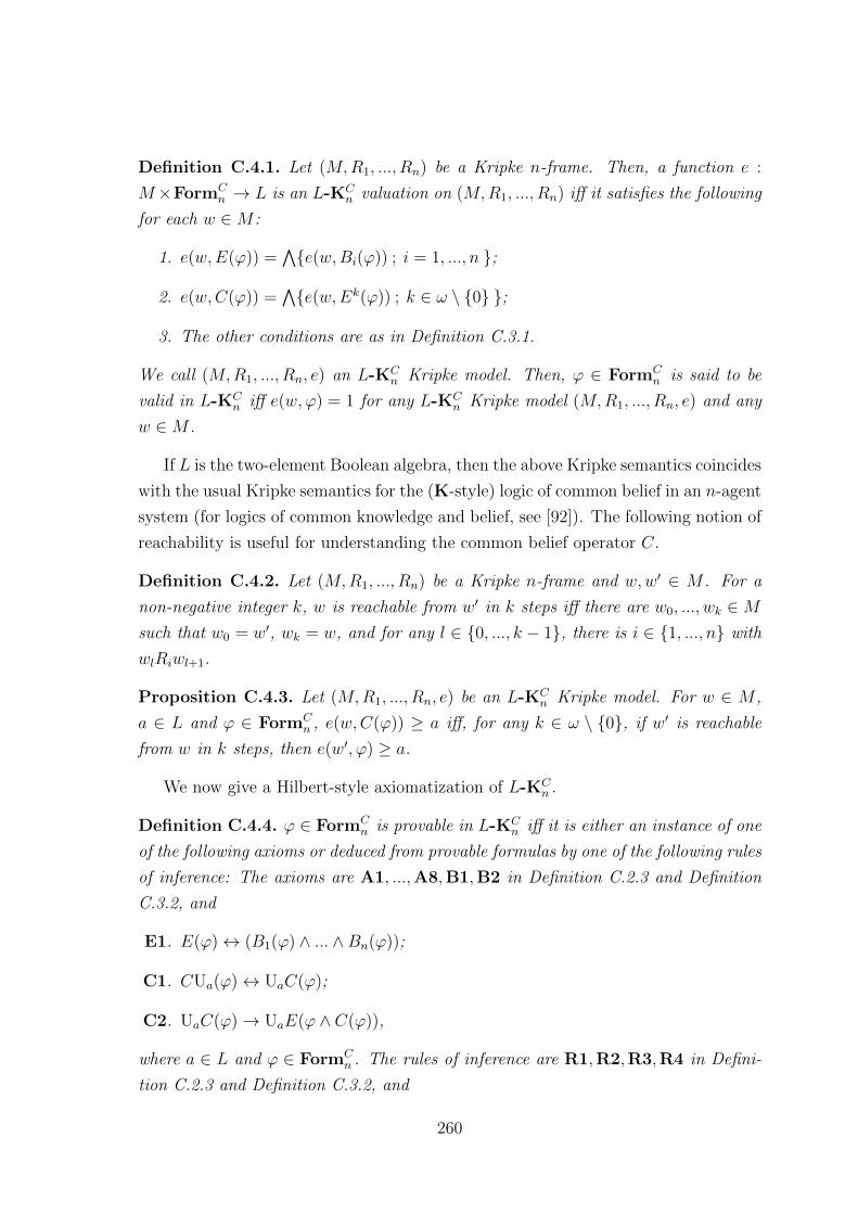
Definition C.4.1. Let (M,R1, ..., Rn) be a Kripke n-frame. Then, a function e :

M×FormCn → L is an L-KC

n valuation on (M,R1, ..., Rn) iff it satisfies the following

for each w ∈M :

1. e(w,E(ϕ)) =∧e(w,Bi(ϕ)) ; i = 1, ..., n ;

2. e(w,C(ϕ)) =∧e(w,Ek(ϕ)) ; k ∈ ω \ 0 ;

3. The other conditions are as in Definition C.3.1.

We call (M,R1, ..., Rn, e) an L-KCn Kripke model. Then, ϕ ∈ FormC

n is said to be

valid in L-KCn iff e(w,ϕ) = 1 for any L-KC

n Kripke model (M,R1, ..., Rn, e) and any

w ∈M .

If L is the two-element Boolean algebra, then the above Kripke semantics coincides

with the usual Kripke semantics for the (K-style) logic of common belief in an n-agent

system (for logics of common knowledge and belief, see [92]). The following notion of

reachability is useful for understanding the common belief operator C.

Definition C.4.2. Let (M,R1, ..., Rn) be a Kripke n-frame and w,w′ ∈ M . For a

non-negative integer k, w is reachable from w′ in k steps iff there are w0, ..., wk ∈Msuch that w0 = w′, wk = w, and for any l ∈ 0, ..., k − 1, there is i ∈ 1, ..., n with

wlRiwl+1.

Proposition C.4.3. Let (M,R1, ..., Rn, e) be an L-KCn Kripke model. For w ∈ M ,

a ∈ L and ϕ ∈ FormCn , e(w,C(ϕ)) ≥ a iff, for any k ∈ ω \ 0, if w′ is reachable

from w in k steps, then e(w′, ϕ) ≥ a.

We now give a Hilbert-style axiomatization of L-KCn .

Definition C.4.4. ϕ ∈ FormCn is provable in L-KC

n iff it is either an instance of one

of the following axioms or deduced from provable formulas by one of the following rules

of inference: The axioms are A1, ...,A8,B1,B2 in Definition C.2.3 and Definition

C.3.2, and

E1. E(ϕ)↔ (B1(ϕ) ∧ ... ∧Bn(ϕ));

C1. CUa(ϕ)↔ UaC(ϕ);

C2. UaC(ϕ)→ UaE(ϕ ∧ C(ϕ)),

where a ∈ L and ϕ ∈ FormCn . The rules of inference are R1,R2,R3,R4 in Defini-

tion C.2.3 and Definition C.3.2, and

260

R5. From ϕ→ E(ϕ ∧ ψ) infer ϕ→ C(ψ).

Using the axioms B1 and B2, we can show the following.

Proposition C.4.5. Let a ∈ L and ϕ ∈ FormCn . (i) EUa(ϕ)↔ UaE(ϕ) is provable

in L-KCn . (ii) E(ϕ ∧ ψ)↔ E(ϕ) ∧ E(ψ) is provable in L-KC

n .

The following theorem states that the above axiomatization of L-KCn is sound and

complete with respect to L-valued Kripke semantics for L-KCn .

Theorem C.4.6. For ϕ ∈ FormCn , ϕ is provable in L-KC

n iff ϕ is valid in L-KCn .

Our proof of the above theorem is rather long and so we put it in the last part of

this section. L-KCn enjoys the finite model property:

Theorem C.4.7. For ϕ ∈ FormCn , ϕ is provable in L-KC

n iff e(w,ϕ) = 1 for any

finite L-KCn Kripke model (M,R1, ..., Rn, e) and any w ∈M .

Proof. The proof of Theorem C.4.6 given below contains the proof of this theorem,

since a counter-model (ConC(ϕ), R1, ..., Rn, e) in the proof of Theorem C.4.6 is actu-

ally a finite L-KCn Kripke model.

By Theorem C.4.6 and Theorem C.4.7, we obtain the decidability of L-KCn .

Theorem C.4.8. For ϕ ∈ FormCn , it is effectively decidable whether or not ϕ is valid

in L-KCn .

Finally, we give the proof of Theorem C.4.6 by generalizing the proof of [92,

Theorem 4.3]

Proof of Theorem C.4.6. It is straightforward to verify the soundness. The complete-

ness is proved as follows. To show the contrapositive, assume that ϕ is not provable

in L-KCn . Let SubC(ϕ) be the set of the following formulas: (i) all subformulas of ϕ;

(ii) B1ψ, ..., Bnψ for each subformula Eψ of ϕ; (iii) ψ ∧ Cψ,B1(ψ ∧ Cψ), ..., Bn(ψ ∧Cψ), E(ψ ∧ Cψ) for each subformula Cψ of ϕ. Let

Sub+C(ϕ) = Ta(ψ),Ua(ψ) ; ψ ∈ SubC(ϕ) and a ∈ L.

Define ConC(ϕ) as the set of all maximal L-KCn consistent subsets of Sub+

C(ϕ). Then,

we can consider the L-KCn Kripke model (ConC(ϕ), R1, ..., Rn, e) such that for each i =

1, ..., n and V,W ∈ ConC(ϕ), V RiW iff, for any a ∈ L and ψ ∈ Sub+C(ϕ), Ua(Biψ) ∈ V

261

implies Ua(ψ) ∈ W and that for each propositional variable p ∈ SubC(ϕ), e(W, p) = a

iff Ta(p) ∈ W . Then we claim that, for a ∈ L, ψ ∈ SubC(ϕ) and W ∈ ConC(ϕ),

e(W,ψ) = a iff Ta(ψ) ∈ W.

If the claim holds, then (ConC(ϕ), R1, ..., Rn, e) is a counter-model for ϕ, since there

is W ∈ ConC(ϕ) with T1(ϕ) /∈ W (i.e., e(W,ϕ) 6= 1) by the assumption that ϕ is

not provable in L-KCn (such W is obtained as follows: Construct a maximal L-KC

n

consistent subset X of FormCn containing ¬T1(ϕ) and then let W = X ∩ Sub+

C(ϕ)).

Thus, to show the completeness, it suffices to verify the claim. Note that the above

claim is equivalent to the following: For a ∈ L with a 6= 0, ψ ∈ SubC(ϕ) and

W ∈ ConC(ϕ), e(W,ψ) ≥ a iff Ua(ψ) ∈ W, since we have: Ta(ψ) ∈ W iff Ux(ψ) ∈ Wfor any x ∈ L with x ≤ a and Ux(ψ) /∈ W for any x ∈ L with x a. We show the

claim by induction on the structure of formulas. We consider only the case that ψ is

of the form C(χ), since arguments in the other cases are similar to those in the proofs

of Theorem C.2.6 and Theorem C.3.3.

Suppose that ψ is of the form C(χ). It suffices to show that, for any W ∈ ConC(ϕ)

and a ∈ L with a 6= 0, e(W,Cχ) ≥ a iff UaC(χ) ∈ W . We first show that UaC(χ) ∈ Wimplies e(W,Cχ) ≥ a. Assume UaC(χ) ∈ W . We claim that, for any k ∈ ω \ 0, if

V ∈ ConC(ϕ) is reachable from W in k steps, then both Ua(χ) and UaC(χ) are in V .

This is shown by induction on k ∈ ω \ 0. We first consider the case k = 1. By C2,

UaC(χ) → UaE(χ ∧ C(χ)) is provable in L-KCn . Then, by W ∈ ConC(ϕ), we have

UaE(χ ∧ C(χ)) ∈ W , whence UaEχ ∈ W and UaE(Cχ) ∈ W by (ii) in Proposition

C.4.5 and (i) in Proposition C.2.7. If V is reachable from W in 1 step, then it follows

from E1 and the definition of Ri that Ua(χ) and UaC(χ) are in V. We next consider

the case k = k′+1 for k′ ∈ ω\0. If V is reachable from W in k′+1 steps, then there

is V ′ ∈ ConC(ϕ) such that V is reachable from V ′ in 1 step and that V ′ is reachable

from W in k′ steps. By the induction hypothesis, both Ua(χ) and UaC(χ) are in V ′.

By arguing as in the case k = 1, it is verified that both Ua(χ) and UaC(χ) are in V .

Thus, the claim has been proved. Hence, for any k ∈ ω \ 0, if V is reachable from

W in k steps, then Ua(χ) ∈ V and so e(V, χ) ≥ a by the induction hypothesis for the

first claim. By Proposition C.4.3, we have e(W,Cχ) ≥ a.

In order to complete the proof, we show that e(W,Cχ) ≥ a implies UaC(χ) ∈ W .

Assume e(W,Cχ) ≥ a. Define

Γ = V ∈ ConC(ϕ) ; e(V,Cχ) ≥ a

ζ =∨∧

V ; V ∈ Γ.

262

where note that both V and ∧V ; V ∈ Γ are finite sets. We first show that

if Ua(ζ) → UaE(χ ∧ ζ) is provable in L-KCn , then UaC(χ) ∈ W . Assume that

Ua(ζ)→ UaE(χ ∧ ζ) is provable in L-KCn . Then, by (i) in Proposition C.4.5 and (i)

in Proposition C.2.7, Ua(ζ)→ E(Ua(χ)∧Ua(ζ)) is provable in L-KCn . Then it follows

from R5 and C1 that Ua(ζ) → UaC(χ) is provable in L-KCn . Since (

∧W ) → ζ

is provable in L-KCn by W ∈ Γ, Ua(

∧W ) → Ua(ζ) is provable in L-KC

n by (ii) in

Proposition C.2.7. By these facts, Ua(∧W ) → UaC(χ) is provable in L-KC

n . Since

Ua(∧W ) ↔ (

∧W ) is provable in L-KC

n by Proposition C.2.8, (∧W ) → UaC(χ)

is provable in L-KCn . Hence, we have UaC(χ) ∈ W . Now it only remains to show

that the assumption of this argument holds, i.e., Ua(ζ)→ UaE(χ ∧ ζ) is provable in

L-KCn .

We have studied the logic of fuzzy belief and common belief with emphasis on

incomparable beliefs (which cannot be formalised in previously known systems in

[33, 91, 114]), establishing completeness and decidability results (implicitly based on

duality-theoretic intuitions). We can also obtain many other versions of the results

such as KD45-style and S5-style ones (and many more). We will study their com-

plexity issues in future work.

We emphasize that our system based on L-valued logic can treat both qualitative

fuzziness and quantitative fuzziness in the context of epistemic reasoning, while sys-

tems based on [0, 1]-valued logic or probabilistic logic (such as those in [33, 91, 114])

can only encompass the latter.

In the previous work such as [186, 191], we studied the mathematically profound

aspects of Fitting’s many-valued modal logic. The results suggest that Fitting’s logic

be beneficial also in the context of artificial intelligence.

We consider that fuzzy reasoning is useful to understand some epistemic problems

such as two generals’ problem or the coordinated attack problem (for this problem,

see, e.g., [92]). In theory, the two generals cannot attack at any time, while, in prac-

tice, they will attack after they have sent messages a few times. We can understand

this as follows. The more times they send messages, the higher the degrees of their

beliefs become. Even if the degrees cannot reach 1, the generals will attack when they

become sufficiently high. This seems to be a very natural understanding of the coor-

dinated attack problem, which is impossible if we stick to classical logic and becomes

possible only if we allow fuzzy reasoning.

We have considered the reduction thesis about belief degrees as being provision-

ally true. Although the reduction thesis would be justified to some degrees by its

263

theoretical merit, in future work, we will discuss in more detail to what extent the

reduction thesis is justifiable, since it would be of philosophical interest as well.

264

Bibliography

[1] S. Abramsky, Domain theory and the logic of observable properties, Ph.D. The-

sis, University of London, 1987.

[2] S. Abramsky, Domain theory in logical form, Ann. Pure Appl. Logic 51 (1991)

1-77.

[3] S. Abramsky, A cook’s tour of the finitary non-well-founded sets, We Will

Show Them: Essays in honour of Dov Gabbay (2005) 1-18 (this is basically a

paper version of an invited talk at the 1988 British Colloquium on Theoretical

Computer Science in Edinburgh).

[4] S. Abramsky, Temperley-Lieb Algebra: From Knot Theory to Logic and Com-

putation via Quantum Mechanics, in: G. Chen, L. Kauffman and S. Lomonaco

(eds.), Mathematics of Quantum Computing and Technology, 515-558, Taylor

and Francis, 2007.

[5] S. Abramsky, Coalgebras, Chu spaces, and representations of physical systems,

Proc. of LICS 2010, pp. 411-420, 2010.

[6] S. Abramsky, Introduction to Categories and Categorical Logic, New Structures

for Physics, pp. 3-94, Springer, 2011.

[7] S. Abramsky, Big toy models: representing physical systems as Chu spaces,

Synthese 186 (2012) 697-718.

[8] S. Abramsky and B. Coecke, A categorical semantics of quantum protocols,

Proc. of LICS’04, pp. 415-425, 2004.

[9] S. Abramsky and B. Coecke, Categorical Quantum Mechanics, Handbook of

Quantum Logic and Quantum Structures, 261-324, Elsevier, 2008.

[10] P. Aczel, Predicate logic with dependent sorts, unpublished manuscript, 2004.

266

[11] J. Adamek, Introduction to coalgebra, Theory and Applications of Categories

14 (2005) 157-199.

[12] J. Adamek, H. Herrlich, and G. E. Strecker, Abstract and Concrete Categories,

John Wiley and Sons, Inc., 1990.

[13] J. Adamek and J. Reiterman, Topological categories presented by small sets of

axioms, Journal of Pure and Applied Algebra 42 (1986) 1-14.

[14] D. Aerts, Quantum axiomatics, Handbook of Quantum Logic and Quantum

Structures, pp. 79-126, 2009.

[15] S. Ambler, First order linear logic and symmetric monoidal closed categories,

PhD thesis, Edinburgh Univ, 1991.

[16] Aristotle, The Metaphysics, Penguin Classics, 1999.

[17] S. Awodey, Category Theory, OUP, 2006.

[18] S. Awodey and H. Forssell, First-Order Logical Duality, Annals of Pure and

Applied Logic 164 (2013) 319-348.

[19] G. Battilotti and P. Zizzi, The internal logic of Bell’s states, arXiv:quant-

ph/0412199.

[20] M. Bacharach, L. A. Gerard-Varet, P. Mongin, and H. S. Shin (eds.), Epistemic

logic and the theory of games and decisions, Springer, 1997.

[21] V. Bargmann, Note on Wigner’s Theorem on Symmetry Operations, Journal

of Mathematical Physics 5 (1964) 862-868.

[22] M. Barr, Autonomous categories, Lecture Notes in Mathematics 752, Springer,

1979.

[23] M. Barr and M. C. Pedicchio, Topological spaces and quasi-varieties, Applied

Categorical Structures 81-85 (1996).

[24] M. Barr, J. F. Kennison and R. Raphael, Isbell duality, Theory and Applications

of Categories 20 (2008) 504-542.

[25] J. Barwise and J. Seligman, Information Flow: The Logic of Distributed Sys-

tems, Cambridge University Press, 1997.

267

[26] J. Beall and G. Restall, Logical Pluralism, OUP, 2006.

[27] J. Bell, Set Theory: Boolean-valued models and independence proofs, 3rd edition,

OUP, 2005.

[28] J. Bell, The Continuous and the Infinitesimal in Mathematics and Philosophy,

Polimetrica, 2005.

[29] N. Belnap, Tonk, Plonk and Plink, Analysis 22 (1962) 130-134.

[30] P. Benacerraf, What Numbers Could Not Be, Philosophical Review 74 (1965)

47-73.

[31] P. Benacerraf, Mathematical Truth, The Journal of Philosophy 70 (1973) 661-

679.

[32] J. van Benthem, Epistemic logic and epistemology: the state of their affairs,

Philosophical Studies 128 (2006) 49-76.

[33] J. van Benthem, J. Gerbrandy and B. Kooi, Dynamic update with probabilities,

Proc. of LOFT’06.

[34] B. von den Berg and C. Heunen, No-go theorems for functorial localic spectra

of noncommutative rings, Proc. of QPL’11, EPTCS, pp. 21-25, 2012.

[35] G. Bezhanishvili, N. Bezhanishvili, D. Gabelaia and A. Kurz, Bitopological

duality for distributive lattices and Heyting algebras, to appear in Mathematical

Structures in Computer Science.

[36] J. M. Bishop, S. J. Nasuto, and B. Coecke, Quantum Linguistics and Searle’s

Chinese Room Argument, Philosophy and Theory of Artificial Intelligence, pp.

17-28, Springer, 2013.

[37] P. Blackburn, M. de Rijke and Y. Venema, Modal logic, CUP, 2001.

[38] V. Boicescu , A. Filipoiu, G. Georgescu and S. Rudeanu, Lukasiewicz-Moisil

algebras, North-Holland Publishing Co., 1991.

[39] D. Bonnay and B. Simmenauer, Tonk Strikes Back, Australasian Journal of

Logic 3 (2005) 33-44.

[40] M. M. Bonsangue, Topological duality in semantics, Electr. Notes Theor. Com-

put. Sci. 8 (1998).

268

[41] M. M. Bonsangue, B. Jacobs, and J. N. Kok, Duality beyond sober spaces:

topological spaces and observation frames, Theor. Comput. Sci. 151 (1995) 79-

124.

[42] V. Boicescu , A. Filipoiu, G. Georgescu and S. Rudeanu, Lukasiewicz-Moisil

algebras, North-Holland Publishing Co., 1991.

[43] F. Bou, F. Esteva and L. Godo, On the minimum many-valued modal logic over

a finite residuated lattice, Journal of Logic and Computation 21 (2011) 739-790.

[44] R. Brandom, Articulating Reasons: An Introduction to Inferentialism, Harvard

University Press, 2000.

[45] C. Brink and I. M. Rewitzky, A paradigm for program semantics: power struc-

tures and duality, CSLI Publications, 2001.

[46] S. Breiner, Scheme representation for first-order logic, Ph.D. Thesis, Carnegie

Mellon University, 2013.

[47] S. Burris and H. P. Sankappanavar, A Course in Universal Algebra, Springer-

Verlag, 1981.

[48] G. C. L. Brummer, Topological categories, Topology and its Applications, 18

(1984) 27-41.

[49] S. Candlish, The Russell/Bradley Dispute and its Significance for Twentieth-

Century Philosophy, Palgrave Macmillan, 2007.

[50] R. Carnap, Meaning and Necessity, 1947.

[51] E. Cassirer, Leibniz’ System in seinen wissenschaftlichen Grundlagen, 1902.

[52] E. Cassirer, Substanzbegriff und Funktionsbegriff, 1910.

[53] E. Cassirer, Philosophie der symbolischen Formen, 1923-1929.

[54] C. C. Chang, Algebraic analysis of many-valued logics, Trans. Amer. Math.

Soc. 88 (1958) 476-490.

[55] C. L. Chang, Fuzzy topological spaces, J. Math. Anal. Appl. 24 (1968) 182-190.

[56] A. Ciabattoni, N. Galatos, and K. Terui, Algebraic Proof Theory for Substruc-

tural Logics, Ann. Pure Appl. Logic 163, pp. 266-290, 2012.

269

[57] R. L. O. Cignoli, E. J. Dubuc, and D. Mundici, Extending Stone duality to

multisets and locally finite MV-algebras, J. Pure Appl. Algebra, 189 (2004)

37-59.

[58] R. L. O. Cignoli, I. M. L. D’Ottaviano and D. Mundici, Algebraic foundations

of many-valued reasoning, Kluwer Academic Publishers, 1999.

[59] A. Chagrov and M. Zakharyaschev, Modal logic, OUP, 1997.

[60] G. Chiribella, G. M. D’Ariano, and P. Perinotti, Informational derivation of

quantum theory, Physical Review A 84, 2011.

[61] P. Cintula, Weakly implicative (fuzzy) logics I: basic properties, Arch. Math.

Log. 45 (2006) 673-704.

[62] C. Cırstea, A. Kurz, D. Pattinson, L. Schroder, and Y. Venema, Modal logics

are coalgebraic, BCS Int. Acad. Conf. (2008) 128-140.

[63] D. M. Clark and B. A. Davey, Natural Dualities for the Working Algebraist,

CUP, 1998. Ann. Math. Artif. Intell. 56 (2009) 339-360.

[64] B. Coecke, Kindergarten Quantum Mechanics, AIP Conference Proceedings 810,

pp. 81-98, American Institute of Physics, 2005.

[65] B. Coecke, Quantum Picturalism, Contemporary Physics 51 (2010) 59-83.

[66] B. Coekce and D. J. Moore, Operational Galois adjunctions, Current Research

in Operational Quantum Logic, pp. 195-218, 2000.

[67] D. Cole, The Chinese Room Argument, The Stanford Encyclopedia of Philoso-

phy, 2009.

[68] R. T. Cook, What’s wrong with tonk(?), Journal of Philosophical Logic 34

(2005) 217-226.

[69] T. Coquand, H. Lombardi, and P. Schuster, Spectral schemes as ringed lattices,

Annals of Mathematics and Artificial Intelligence, 2009.

[70] D. Coumans, M. Gehrke, and L. van Rooijen, Relational Semantics for Full

Linear Logic, Journal of Applied Logic 12, pp. 50-66, 2014.

[71] W. A. Coppel, Foundations of Convex Geometry, CUP, 1998.

270

[72] B. A. Davey and H. A. Priestley, Introduction to Lattices and Order, CUP, 2002.

[73] B. A. Davey, V. J. Schumann, and H. Werner, From the subalgebra of the

square to the discriminator, Algebra Universalis 28 (1991) 500-519.

[74] J. Dauns and K. Hofmann, The representation of biregular rings by sheaves.

Math. Z 91, pp. 103-123, 1966.

[75] D. Davidson, Inquiries into Truth and Interpretation, Clarendon Press, 2001.

[76] B. W. Davis, The Kyoto School, Stanford Encyclopedia of Philosophy, 2010.

[77] D. Dennett, Toward a Cognitive Theory of Consciousness, Brainstorms: Philo-

sophical Essays on Mind and Psychology, pp. 149-173, MIT Press, 1978.

[78] J. Derrida, De la grammatologie, Les Editions de Minuit, 1967.

[79] D. Deutsch, The Fabric of Reality, Penguin, 1997.

[80] M. Devitt, Realism and Truth, 2nd Edition, Princeton University Press, 1991.

[81] G. Dimov and W. Tholen, A characterization of representable dualities, Cate-

gorical Topology and its Relations to Analysis, Algebra and Combinatorics, J.

Adamek and S. MacLane (eds.), World Scientific, pp. 336-357, 1989.

[82] R. S. Doran and V. A. Belfi, Characterizations of C∗-algebras; The Gelfand-

Naimark theorems, Marcel Dekker Inc., New York and Basel, 1986.

[83] A. Doring, Generalised Gelfand Spectra of Nonabelian Unital C∗-Algebras,

arXiv:1212.2613.

[84] K. Dosen, Logical Constants: An Essay in Proof Theory, D. Phil. Thesis, Oxford

University, 1980.

[85] K. Dosen, Logical Constants as Punctuation Marks, Notre Dame Journal of

Formal Logic 30 (1989) 362-381.

[86] M. Dummett, Truth and Other Enigmas, Duckworth, 1978.

[87] M. Dummett, The Logical Basis of Metaphysics, Duckworth, 1991.

[88] R. Engelking, General Topology, Heldermann Verlag, 1989.

[89] L. Esakia, Topological Kripke models, Soviet Math. Dokl. 15 (1974) 147-151.

271

[90] C. Faggian and G. Sambin, From Basic Logic to Quantum Logics with Cut-

Elimination, International Journal of Theoretical Physics 37, pp. 31-37, 1998.

[91] R. Fagin and J. Y. Halpern, Reasoning about knowledge and probability, Jour-

nal of the ACM 41 (1994) 340-367.

[92] R. Fagin, J. Y. Halpern, Y. Moses and M. Y. Vardi, Reasoning about knowledge,

MIT press, 1995.

[93] M. C. Fitting, Many-valued modal logics, Fundam. Inform. 15 (1991) 235-254.

[94] M. C. Fitting, Many-valued modal logics II, Fundam. Inform. 17 (1992) 55-73.

[95] M. C. Fitting, Many-valued non-monotonic modal logics, Proc. of LFCS’92,

Springer LNCS 620, 139-150.

[96] M. C. Fitting, Tableaus for many-valued modal logic, Studia Logica 55 (1995)

63-87.

[97] S. French, The Structure of the World, OUP, 2014.

[98] J. Frey, A 2-Categorical Analysis of the Tripos-to-Topos Construction,

arXiv:1104.2776.

[99] M. Friedman, Reconsidering Logical Positivism, CUP, 1999.

[100] M. Friedman, A Parting of the Ways: Carnap, Cassirer, and Heidegger, Open

Court, 2000.

[101] M. Friedman, Dynamics of Reason, Stanford University Press, 2001.

[102] T. Fritz, Convex Spaces I: Definition and Examples, arXiv:0903.5522.

[103] R. Furber and B. Jacobs, From Kleisli categories to commutative C∗-algebras:

Probabilistic Gelfand duality, Proc. of CALCO’13, Springer LNCS, pp 141-157,

2013.

[104] N. Galatos, P. Jipsen, T. Kowalski, and H. Ono, Residuated Lattices: An Alge-

braic Glimpse at Substructural Logics, Elsevier, 2007.

[105] P. Galison and D. Stump (eds.), The Disunity of Science, SUP, 1996.

[106] N. Gambino and P. Aczel, The generalized type-theoretic interpretation of con-

structive set theory, Journal of Symbolic Logic 71 (2006) 67-103.

272

[107] M. Gehrke and J. Harding, Bounded lattice expansions, J. Algebra 239 (2001)

345-371.

[108] M. Gehrke, H. Nagahashi and Y. Venema, A Sahlqvist theorem for distributive

modal logic, Ann. Pure Appl. Logic 131 (2005) 65-102.

[109] G. Gierz, K. H. Hofmann, K. Keimel, J. D. Lawson, M. W. Mislove, and D. S.

Scott, Continuous Lattices and Domains, CUP, 2003.

[110] J.-Y. Girard, Linear Logic, Advances in Linear Logic, CUP, 1995.

[111] J.-Y. Girard, Y. Lafont, and P. Taylor, Proofs and Types, CUP, 1989.

[112] E. Giuli and W. Tholen, A topologist’s view of Chu spaces, Applied Categorical

Structures, (2007) 573-598.

[113] K. Godel, Collected Works, Volume III, Oxford University Press, 1981.

[114] L. Godo, P. Hajek, and F. Esteva, A fuzzy modal logic for belief functions,

Fundamenta Informaticae 57 (2003) 127-146.

[115] J. A. Goguen, L-fuzzy sets, J. Math. Anal. Appl. 18 (1967) 145-174.

[116] J. A. Goguen, The fuzzy Tychonoff theorem, J. Math. Anal. Appl. 43 (1973)

734-742.

[117] A Goguen and J Meseguer, Completeness of many-sorted equational logic, ACM

SIGPLAN Notices 17 (1982) 9-17.

[118] S. Gottwald, A treatise on many-valued logics, Research Studies Press, 2001.

[119] R. Goldblatt. Mathematics of modality, CSLI Lecture Notes 43, Stanford, 1993.

[120] S. Gottwald, A treatise on many-valued logics, Research Studies Press, 2001.

[121] G. A. Gratzer, Universal algebra, Springer-Verlag, 1979.

[122] R. Grigolia, Algebraic analysis of Lukasiewicz-Tarski n-valued logical systems,

Selected papers on Lukasiewicz sentential calculi, Wroclaw, pp. 81-91, 1977.

[123] A. Grothendieck and J. Dieudonne, Elements de geometrie algebrique (rediges

avec la collaboration de Jean Dieudonne) : I. Le langage des schemas, Publica-

tions Mathematiques de l’IHES 4 (1960) 5-228.

273

[124] P. M. Gruber and J. M. Wills (eds.), Handbook of Convex Geometry Vol. A. B,

North-Holland, 1993.

[125] P. Hajek, Metamathematics of fuzzy logic, Kluwer Academic Publishers, 1998.

[126] P. Hajek and P. Cintula, On theories and models in fuzzy predicate logics, J.

Symb. Log. 71, pp. 863-880, 2006.

[127] G. Hansoul, A duality for Boolean algebras with operators, Algebra Universalis

17 (1983) 34-49.

[128] G. Hansoul and B. Teheux, Completeness results for many-valued Lukasiewicz

modal systems and relational semantics, preprint, arXiv:math/0612542v1.

[129] R. Hartshorne, Algebraic Geometry, Springer, 1977.

[130] H. Herbelin, A λ-calculus Structure Isomorphic to Gentzen-style Sequent Cal-

culus Structure, Computer Science Logic, Springer LNCS, 61-75, 1995.

[131] M. Heidegger, Sein und Zeit, 1927.

[132] C. Heunen and B. Jacobs, Quantum logic in dagger kernel categories, Order 27,

pp. 177-212, 2010.

[133] D. Hilbert, On the Infinite, in: J. van Heijenoort (ed.), From Frege to Godel:

A Source Book in Mathematical Logic, 1897-1931, 369-92, Harvard University

Press, 1967.

[134] J. Hintikka, Knowledge and belief - an introduction to the logic of the two no-

tions, Cornell University Press, 1962.

[135] K. H. Hofmann, M. Mislove and A. Stralka, The Pontryagin Duality of Compact

0-Dimensional Semilattices and its Applications, Lecture Notes in Math. 394,

Springer, 1974.

[136] R.-E. Hoffmann, On the sobrification remainder sX − X, Pacific J. Math. 83

(1979) 145-156.

[137] K. H. Hofmann, Representation of algebras by continuous sections, Bull. Amer.

math. Soc. 78, pp. 291-373, 1972.

[138] U. Hohle and T. Kubiak, A non-commutative and non-idempotent theory of

quantale sets, Fuzzy Sets and Systems 166, pp. 1-43, 2011.

274

[139] T. K. Hu, Stone Duality for primal algebra theory, Math. Z. 110 (1969) 180-198.

[140] T. K. Hu, On the topological duality for primal algebra theory, Algebra Uni-

versalis 1 (1971), 152-154.

[141] P. Hut and B. van Fraassen, Elements of reality: a dialogue, Journal of Con-

sciousness Studies 4 (1997) 167-80.

[142] H. Huwig and A. Poigne, A Note on Inconsistencies Caused by Fixpoints in a

Cartesian Closed Category, Theoretical Computer Science 73 (1990) 101-112.

[143] M. Hyland, P. T. Johnstone, and A. Pitts, Tripos Theory, Math. Proc. Cam-

bridge Philos. Soc. 88, pp. 205-232, 1980.

[144] J. R. Isbell, General functorial semantics, Amer. J. Math. 94 (1972) 535-596.

[145] B. Jacobs, Categorical Logic and Type Theory, Elsevier, 1999.

[146] B. Jacobs, Convexity, Duality, and Effects, Proc. of 6th IFIP International

Conference on Theoretical Computer Science (2010) 1-19.

[147] B. Jacobs, New directions in categorical logic, arXiv:1205.3940v2.

[148] B. Jacobs and J. Rutten, A tutorial on (co)algebras and (co)induction, Bulletin

of EATCS 62 (1997) 229-259.

[149] P. T. Johnstone, Stone Spaces, CUP, 1986.

[150] P. T. Johnstone, Sketches of an Elephant, OUP, 2002.

[151] B. Jonsson and A. Tarski, Boolean algebras with operators I, Amer. J. of Math.

73 (1951) 891-939.

[152] R. Kahle, and P. Schroder-Heister (eds.), Proof-Theoretic Semantics, special

issue of Synthese (vol. 148), Springer, 2005.

[153] C. Kaner, J. Falk, and H. Q. Nguyen, Testing Computer Software, 2nd ed,

Wiley, 1999.

[154] K. Keimel and H. Werner, Stone duality for varieties generated by a quasi-

primal algebra, Mem. Amer. Math. Soc. 148 (1974) 59-85.

[155] K. Keimel, Sheaf representations for algebraic systems. A personal historical

account, arXiv:1308.6249.

275

[156] R. L. Kirkham, Theories of Truth, MIT Press, 1995.

[157] B. Klin, Coalgebraic modal logic beyond sets, Electr. Notes Theor. Comput.

Sci. 173 (2007) 177-201.

[158] A. Knoebel, Sheaves of Algebras over Boolean Spaces, Birkhauser, 2012.

[159] C. Kupke, A. Kurz and Y. Venema, Stone coalgebras, Theor. Comput. Sci. 327

(2004) 109-134 (this is an extended version of Electr. Notes Theor. Comput.

Sci. 82 (2003) 170-190).

[160] A. Kurz and D. Petrisan, Presenting functors on many-sorted varieties and

applications, Information and Computation 208 (2010) 1421-1446.

[161] S. Kripke. Naming and Necessity, 1972.

[162] S. Kripke, Wittgenstein on Rules and Private Language, Harvard University

Press, 1982.

[163] A. Kurz, Coalgebras and their logics, SIGACT News 37 (2006) 57-77.

[164] A. Kurz and J. Velebil, Enriched logical connections, to appear in Applied Cat-

egorical Structures.

[165] J. Ladyman, Structural Realism, Stanford Encyclopedia of Philosophy, 2014.

[166] J. Ladyman and D. Ross, with D. Spurrett and J. Collier, Every Thing Must

Go: Metaphysics Naturalized, OUP, 2007.

[167] J. Lambek, On the representation of modules by sheaves of factor modules,

Canad. Math. Bull. 14, pp. 359-368, 1971.

[168] J. Lambek and P. J. Scott, Introduction to Higher-Order Categorical Logic,

1986.

[169] S. Lloyd, Programming the Universe: A Quantum Computer Scientist Takes on

the Cosmos, Knopf, 2006.

[170] R. Landauer, Information is physical, Physics Today, pp. 23-9, 1991.

[171] F. W. Lawvere, Adjointness in Foundations, Dialectica 23, pp. 281-296, 1969.

Reprinted with the author’s retrospective commentary in: Theory and Appli-

cations of Categories 16, pp. 1-16, 2006.

276

[172] F. W. Lawvere, Equality in hyperdoctrines and comprehension scheme as an

adjoint functor, Application of Categorical Algebra, pp. 1-14, 1970.

[173] W. Lawvere, Categories of space and quantity, The Space of mathematics, de

Gruyter, pp. 14-30, 1992.

[174] L. Leustean, Sheaf representations of BL-algebras, Soft Computing 9 (2005)

897-909.

[175] Y. M. Liu and M. K. Luo, Fuzzy topology, World Scientific, 1998.

[176] J. Lukasiewicz and A. Tarski, Untersuchungen uber den Assagenkalkul, Compt.

Rend. des Seances Societe des Sciences et Lettres de Varsovie Classe III 23

(1930) 3-50.

[177] J. Lurie, Higher Topos Theory, Princeton University Press, 2009.

[178] S. Luft, The Space of Culture: Towards a Neo-kantian Philosophy of Culture -

Cohen, Natorp, and Cassirer, OUP, 2015.

[179] W. G. Lycan, Philosophy of Language, Routledge, 2008.

[180] J.-F. Lyotard, La condition postmoderne: rapport sur le savoir, Les Editions de

Minuit, 1979.

[181] G. Malinowski, Many-valued logics, Clarendon Press, 1993.

[182] A. Magid, Pierce’s representation and separable algebras, Illinois J. Math. 15,

pp. 114-121, 1971.

[183] E. G. Manes, Algebraic Theories, Springer, 1976.

[184] J.-P. Marquis and G. Reyes, The History of Categorical Logic: 1963-1977, in:

Handbook of the History of Logic, Vol. 6, pp. 689-800, Elsevier, 2011.

[185] P. Martin-Lof, On the Meanings of the Logical Constants and the Justifications

of the Logical Laws, Nordic Journal of Philosophical Logic 1 (1996) 11-60.

[186] Y. Maruyama, Algebraic study of lattice-valued logic and lattice-valued modal

logic, Lecture Notes in Computer Science 5378 (2009) 172-186.

[187] Y. Maruyama, A duality for algebras of lattice-valued modal logic, Lecture

Notes in Computer Science 5514 (2009) 281-295.

277

[188] Y. Maruyama, Fuzzy topology and Lukasiewicz logics from the viewpoint of

duality theory, Studia Logica 94 (2010) 245-269.

[189] Y. Maruyama, Fundamental results for pointfree convex geometry, Ann. Pure

Appl. Logic 161 (2010) 1486-1501.

[190] Y. Maruyama, Dualities for algebras of Fitting’s many-valued modal logics,

Fundam. Inform. 106 (2011) 273-294.

[191] Y. Maruyama, Categorical duality between two aspects of the notion of space,

Master thesis, Kyoto University, 2011.

[192] Y. Maruyama, Natural duality, modality, and coalgebra, Journal of Pure and

Applied Algebra, pp. 565-580, 2012.

[193] Y. Maruyama, From operational Chu duality to coalgebraic quantum symmetry,

Proc. of CALCO’13, Springer LNCS, pp. 220-235, 2013.

[194] Y. Maruyama, Full Lambek Hyperdoctrine, Springer LNCS 8071, pp.211-225,

2013.

[195] Y. Maruyama, Categorical duality theory: domains, convexity, and the distri-

bution monad, Proc. of CSL’13, LIPICS, pp. 500-520, 2013.

[196] Y. Maruyama, Quantum Linguistics: From Philosophy of Language to Logic of.

Quantum Vagueness, Proceedings of the Tenth International Workshop of Logic

and Engineering of Natural Language Semantics 10, JSAI, pp. 28-41, 2013.

[197] Y. Maruyama, Wittgenstein’s Conception of Space and the Modernist Trans-

formation of Geometry via Duality, Papers of 36th International Wittgenstein

Symposium, Austrian Wittgenstein Society, 2013.

[198] Y. Maruyama, Duality Theory and Categorical Universal Logic, Proc. of Quan-

tum Physics and Logic, EPTCS 171, pp. 100-112, 2014.

[199] Y. Maruyama, Categorical Harmony and Paradoxes in Proof-Theoretic Seman-

tics, Advances in Proof-Theoretic Semantics, pp. 95-114, 2016.

[200] Y. Maruyama, AI, Quantum Information, and External Semantic Realism:

Searles Observer-Relativity and Chinese Room, Revisited, Synthese Library,

376, Springer, pp. 115-126, 2016.

278

[201] Y. Maruyama, Prior’s tonk, notions of logic, and levels of inconsistency: vindi-

cating the pluralistic unity of science in the light of categorical logical positivism,

Synthese (forthcoming; already published online).

[202] Y. Maruyama, Dynamics of Duality, forthcoming.

[203] Y. Maruyama and K. Sato, Intuitionistic many-valued logic and its geometric

duality, preprint (chapter in Sato’s PhD thesis at Kobe University).

[204] E. Michael, Topologies on spaces of subsets, Trans. Amer. Math. Soc. 71 (1951)

152-182.

[205] A. Miller, The significance of semantic realism, Synthese 136 (2003) 191-217.

[206] A. Miller, Realism, The Stanford Encyclopedia of Philosophy, 2010.

[207] L. Molnar, An Algebraic Approach to Wigner’s Unitary-Antiunitary Theorem,

arXiv:math/9808033.

[208] D. J. Moore, On state spaces and property lattices, Stud. Hist. Phil. Mod. Phys.

30 (1999) 61-83.

[209] P. Niederkorn, Natural dualities for varieties of MV-algebras, J. Math. Anal.

Appl. 255 (2001) 58-73.

[210] A. Nishi, Interweaving a Hundred Sciences, 1870.

[211] K. Nishitani et al., Overcoming Modernity, 1942.

[212] A. Di Nola and P. Niederkorn, Natural dualities for varieties of BL-algebras,

Arch. Math. Log. 44 (2005) 995-1007.

[213] A. Jung and M. A. Moshier, On the bitopological nature of Stone Duality.

Technical Report CSR-06-13, School of Computer Science, University of Birm-

ingham, 2006.

[214] I. D. Nel and R. G. Wilson, Epireflections in the category of T0 spaces, Fund.

Math. 75 (1972) 69-74.

[215] P. Niederkorn, Natural dualities for varieties of MV-algebras, J. Math. Anal.

Appl. 225 (2001) 58-73.

[216] K. Nishida, An inquiry into the good, Yale University Press, 1990.

279

[217] J. C. Maraldo, Nishida Kitaro, Stanford Encyclopedia of Philosophy, 2012.

[218] I. Ojima,. Micro-macro duality in quantum physics, Stochastic Analysis: Clas-

sical and Quantum, pp. 143-161, 2005.

[219] H. Ono, Algebraic semantics for predicate logics and their completeness, RIMS

Kokyuroku 927, pp. 88-103, 1995.

[220] H. Ono, Substructural logics and residuated lattices - an introduction, 50 Years

of Studia Logica, Trends in Logic, Kluwer Academic Publishers, 21 (2003) 193-

228.

[221] H. Ono, Crawley Completions of Residuated Lattices and Algebraic Complete-

ness of Substructural Predicate Logics, Studia Logica 100, pp. 339-359, 2012.

[222] P. Ostermann, Many-valued modal propositional calculi, Z. Math. Logik Grund-

lag. Math. 34 (1988) 343-354.

[223] M. Ozawa, Transfer principle in quantum set theory, J. Symbolic Logic 72 (2007)

625-648.

[224] A. Palmigiano and Y. Venema, Nabla algebras and Chu spaces, In Mossakowski

et al. [18], pages 394-408.

[225] J. W. Pelletier and J. Rosicky, Generating the equational theory of C∗-algebras

and related categories, Proc. of Conference on Categorical Topology (1989) 163-

180.

[226] G. Piccinini, Computation in Physical Systems, The Stanford Encyclopedia of

Philosophy, 2010.

[227] R. Pierce, Modules over commutative regular rings, Mem. Amer. Math. Soc 70,

1967.

[228] J. Pitkethly and B. Davey, Dualisability: unary algebras and beyond, Springer,

2005.

[229] A. Pitts, Categorical Logic, in: Handbook of Logic in Computer Science, Vol. 5,

Chap. 2, OUP, 2000.

[230] A. Pitts, Tripos Theory in Retrospect, Mathematical Structures in Computer

Science 12, pp. 265-279, 2002.

280

[231] A. F. Pixely, The ternary discriminator function in universal algebra, Math.

Ann. 191 (1971) 167-180.

[232] H.-E. Porst and W. Tholen, Concrete dualities, Category Theory at Work (1991)

111-136.

[233] M. B. Pour-El and S. Kripke, Deduction-preserving “Recursive Isomorphisms”

between Theories, Fundamenta Mathematicae 61 (1967) 141-163.

[234] V. R. Pratt, The Stone Gamut: a coordinatization of mathematics, Proc. of

LICS 1995, pp. 444-454.

[235] V. R. Pratt, Chu Spaces, Notes for School on Category Theory and Applications,

University of Coimbra, Portugal, July 13-17, 1999.

[236] D. Prawitz, Natural Deduction, Almqvist & Wiksell, 1965.

[237] D. Prawitz, Ideas and Results in Proof Theory, in: Proceedings of the Second

Scandinavian Logic Symposium, 235-307, North-Holland, Amsterdam, 1971.

[238] G. Priest, Paraconsistent Logic, Handbook of Philosophical Logic 6, 287-393,

2002.

[239] H. A. Priestley, Ordered topological spaces and the representation of distribu-

tive lattices, Proc. London Math. Soc. 24 (1972) 507-530.

[240] H. A. Priestley, Representation of distributive lattices by means of ordered stone

spaces, Bull. London Math. Soc. 2, 186-190.

[241] H. A. Priestley, Varieties of distributive lattices with unary operations I, J.

Austral. Math. Soc. Ser. A 63 (1997) 165-207.

[242] A. N. Prior, The Runabout Inference-Ticket, Analysis 21 (1960) 38-39.

[243] W. V. Quine, Theories and Things, Harvard University Press, 1981.

[244] S. E. Rodabaugh and E. P. Klement (eds.), Topological and algebraic structures

in fuzzy sets, Kluwer Academic Publishers, 2003.

[245] J. J. M. M. Rutten, Universal coalgebra: a theory of systems, Theor. Comput.

Sci. 249 (2000) 3-80.

281

[246] G. Sambin, G. Battilotti, and C. Faggian, Basic Logic: Reflection, Symmetry,

Visibility, Journal Symbolic Logic 65 (2000) 979-1013.

[247] G. Sambin, The Basic Picture: Structures for Constructive Topology, Oxford

University Press, to appear.

[248] G. Sambin and V. Vaccaro, Topology and duality in modal logic, Ann. Pure

Appl. Logic 37 (1988) 249-296.

[249] J. E. Santo, Revisiting the Correspondence between Cut Elimination and Nor-

malisation, Automata, Languages and Programming, Springer LNCS, 600-611,

2000.

[250] J. Searle, The Rediscovery of the Mind, Cambridge, MIT Press, 1992.

[251] J. Searle, Mind, Language, and Society: Philosophy in the Real World, Basic

Books, 1998.

[252] J. Searle, The Problem of Consciousness, Consciousness and Language, pp.

7-17, Cambridge University Press, 2002.

[253] S. Shapiro, Varieties of Logic, OUP, 2014.

[254] Y. Shoham and K. Leyton-Brown, Multiagent systems: algorithmic, game-

theoretic, and logical foundations, CUP, 2009.

[255] P. Schroeder-Heister, Proof-Theoretic Semantics, Stanford Encyclopedia of Phi-

losophy, 2012.

[256] P. Schroeder-Heister, Definitional Reflection and Paradoxes, Supplement to

[255], Stanford Encyclopedia of Philosophy, 2012.

[257] P. Schroeder-Heister, Proof-Theoretic Semantics, Self-Contradiction, and the

Format of Deductive Reasoning, Topoi 31 (2012) 77-85.

[258] P. Schroeder-Heister, The Categorical and the Hypothetical: A Critique of

Some Fundamental Assumptions of Standard Semantics, Synthese 187 (2012)

925-942.

[259] A. P. Sostak, Basic structures of fuzzy topology, Journal of Mathematical Sci-

ences 78 (1996) 662-701.

282

[260] A. Stairs, Could Logic be Empirical? The Putnam-Kripke Debate, forthcoming

in: J. Chubb, A. Eskandarian, and V. Harizanov (eds.), Logic and Algebraic

Structures in Quantum Computing and Information, CUP, 2014.

[261] M. H. Stone, Topological representation of distributive lattices and Brouwerian

logic, Casopis pest. Mat. a Fys. 67 (1937), 1-25.

[262] M. H. Stone, The representation of Boolean algebras, Bull. Amer. Math. Soc.

44 (1938) 807-816.

[263] B. Spitters, S. Vickers, and S. Wolters, Gelfand spectra in Grothendieck toposes

using geometric mathematics, arXiv:1310.0705

[264] M. R. Talukder, Natural duality theory with applications to Heyting algebras

and generalised modal algebras, Ph.D. thesis, La Trobe University, 2002.

[265] B. Teheux, A duality for the algebras of a Lukasiewicz n + 1-valued modal

system, Studia Logica 87 (2007) 13-36.

[266] G. Takeuti, Quantum set theory, Current Issues in Quantum Logic, pp. 303-322,

1981.

[267] D. Turi and J. Rutten, On the foundations of final coalgebra semantics: non-

well-founded sets, partial orders, metric spaces, Math. Struct. in Comput. Sci.

8 (1998) 481-540.

[268] A. Turing, Computing Machinery and Intelligence, Mind 49 (1950) 433-460.

[269] E. Vailati, Leibniz and Clarke: A Study of Their Correspondence, OUP, 1997.

[270] M. L. J. van de Vel, Theory of Convex Structures, North-Holland, 1993.

[271] S. Vickers, Topology via Logic, Cambridge University Press, 1996.

[272] N. de Warren and A. Staiti (eds.), New Approaches to Neo-Kantianism, Cam-

bridge University Press, 2015.

[273] A. Weil, Foundations of Algebraic Geometry, American Mathematical Society

Colloquium Publications 29, 1946.

[274] A. Weil, Basic Number Theory, Springer, 2013.

283

[275] D. Westerstahl, From Constants to Consequence, and Back, Synthese 187 (2012)

957-971.

[276] J. A. Wheeler, Information, Physics, Quantum: the Search for Links, Com-

plexity, Entropy, and the Physics of Information, pp. 309-336, Addison-Wesley,

1990.

[277] A. N. Whitehead, Process and Reality, 1929.

[278] E. P. Wigner, Gruppentheorie, Friedrich Vieweg und Sohn, pp. 251-254, 1931

(English translation: Group Theory, Academic Press Inc., pp. 233-236, 1959).

[279] L. Wittgenstein, Tractatus Logico-Philosophicus, 1921.

[280] L. Wittgenstein, Philosophical Investigations, 1953.

[281] L. Wittgenstein, Philosophical Remarks, 1964

[282] L. Wittgenstein, Philosophical Grammar, 1974.

[283] Y. Xu, D. Ruan, K. Qin, and J. Liu, Lattice-valued logic: an alternative ap-

proach to treat fuzziness and incomparability, Springer, 2003.

[284] L.A. Zadeh, Fuzzy sets, Information and Control 8 (1965) 338-353.

[285] P. Zizzi, Basic logic and quantum entanglement, J. Phys.: Conf. Ser. 67,

012045, 2007.

[286] J. Zucker, The Correspondence between Cut-Elimination and Normalization,

Annals of Mathematical Logic 7 (1974) 1-112.

284