measurement and modelling of atmospheric acoustic
TRANSCRIPT

DEFENCE DÉFENSE&
Defence Research andDevelopment Canada
Recherche et développementpour la défense Canada
Measurement and Modelling of Atmospheric
Acoustic Propagation Over Water
Cristina Tollefsen
E. C. Murowinski
Sean Pecknold
Technical Memorandum
DRDC Atlantic TM 2010-184
December 2010
Defence R&D Canada – Atlantic
Copy No. _____

This page intentionally left blank.

Measurement and Modelling of AtmosphericAcoustic Propagation Over Water
Cristina Tollefsen
Defence R&D Canada – Atlantic
E. C. Murowinski
Defence R&D Canada – Atlantic
Sean Pecknold
Defence R&D Canada – Atlantic
Defence R&D Canada – AtlanticTechnical Memorandum
DRDC Atlantic TM 2010-184
December 2010

Principal Author
Cristina Tollefsen
Approved by
Daniel HuttHead/Underwater Sensing
Approved for release by
Calvin HyattHead/Document Review Panel
c© Her Majesty the Queen in Right of Canada as represented by the Minister of NationalDefence, 2010
c© Sa Majeste la Reine (en droit du Canada), telle que representee par le ministre de laDefense nationale, 2010

Abstract
General interest in understanding atmospheric acoustic propagation over water has in-creased in recent years, driven primarily by concerns about noise from offshore wind farms.In addition, there are specific naval interests such as evaluating the performance of direc-tional acoustic hailing devices used at sea, determining the potential environmental impactof naval gunfire exercises, and understanding the in-air acoustic footprint of maritime-based military assets. Atmospheric acoustic propagation is strongly affected by the envi-ronment, including sea surface roughness and atmospheric parameter profiles (temperature,wind velocity, humidity, and turbulence). However, published measurements and realisticmodelling of the effect of environmental parameters on over-water acoustic propagationare sparse. An experiment was designed to measure atmospheric acoustic transmissionloss over water by using an acoustic source on a small boat and a receiver on a barge.Point measurements of atmospheric parameters and directional ocean wave spectra weremade in the vicinity the experiment. Also, separate data from two types of atmosphericparameter profiles - measured radiosonde profiles and modelled profiles generated by En-vironment Canada’s Global Environmental Multiscale (GEM) model - were made availablefor this investigation. The dependence of measured transmission loss on source-to-receiverrange, atmospheric parameter profiles, receiver height, and wind speed was explored, andimpulsive sources were used to observe separate multipath arrivals. Measured acoustictransmission loss was compared with the output of the Sensor Performance Evaluator forBattlefield Environments (SPEBE) atmospheric acoustic propagation model developed bythe United States’ Army Research Laboratory (ARL).
Resume
Depuis quelques annees, on s’interesse de plus en plus a l’etude de la propagation acous-tique au-dessus de l’eau, en raison surtout des preoccupations relatives au bruit provenantdes parcs eoliens en mer. On souhaite en outre, dans le secteur de la Marine, evaluer la per-formance des dispositifs d’appels acoustiques directionnels pour usage en mer, determinerl’impact environnemental possible des exercices de l’artillerie navale et comprendre l’em-preinte acoustique dans l’air des ressources militaires maritimes. La propagation acoustiqueatmospherique est tres sensible a l’environnement, y compris les profils des parametres at-mospheriques (temperature, vitesse du vent, humidite et turbulence) et la rugosite de la sur-face. Par contre, peu de donnees ont ete publiees sur les mesures et la modelisation realistedes effets des parametres environnementaux sur la propagation acoustique au-dessus del’eau. Une experience a ete concue pour mesurer les pertes de transmission acoustiqueau-dessus de l’eau au moyen d’une source acoustique installee sur un petit bateau et derecepteurs installes sur un chaland. Des mesures par points des parametres atmospheriqueset spectres de vagues directionnelles oceaniques ont ete effectuees aux environs du sitede l’experience. De plus, d’autres donnees de deux types de profil des parametres at-
DRDC Atlantic TM 2010-184 i

mospheriques - des profils de radiosonde mesures et des profils modelises produits parle modele global environnementale multi-echelle (GEM) d’Environnement Canada - ontete utilisees pour cette recherche. On s’est penche sur le rapport entre les pertes de trans-mission mesurees et la distance entre la source et le recepteur, les profils des parametresatmospheriques, la hauteur du recepteur et la vitesse du vent, et on a employe des sourcesimpulsives pour observer des receptions distinctes par trajets multiples. Les pertes de trans-mission acoustique mesurees ont ete comparees aux resultats de l’evaluateur des perfor-mances de capteurs pour les environnements de combat (SPEBE), un modele de propaga-tion acoustique atmospherique mis au point par l’ARL (Army Research Laboratory) desEtats-Unis.
ii DRDC Atlantic TM 2010-184

Executive summary
Measurement and Modelling of Atmospheric AcousticPropagation Over Water
Cristina Tollefsen, E. C. Murowinski, Sean Pecknold; DRDC Atlantic
TM 2010-184; Defence R&D Canada – Atlantic; December 2010.
Background: General interest in understanding atmospheric acoustic propagation overwater has increased in recent years, driven primarily by concerns about noise from off-shore wind farms. In addition, there are specific naval interests such as evaluating theperformance of directional acoustic hailing devices used at sea, determining the poten-tial environmental impact of naval gunfire exercises, and understanding the in-air acousticfootprint of maritime-based military assets. Atmospheric acoustic propagation is stronglyaffected by the environment, including sea surface roughness and atmospheric parameterprofiles (temperature, wind velocity, humidity, and turbulence). However, published mea-surements and realistic modelling of the effect of environmental parameters on over-wateracoustic propagation are sparse.
Principal results: An experiment was designed to measure atmospheric acoustic transmis-sion loss over water by using an acoustic source on a small boat and a receiver on a barge.Point measurements of atmospheric parameters and directional ocean wave spectra weremade in the vicinity the experiment. Additional environmental data available include twotypes of atmospheric parameter profiles: measured radiosonde profiles, and modelled pro-files generated by Environment Canada’s Global Environmental Multiscale (GEM) model.The dependence of measured transmission loss on source-to-receiver range, atmosphericparameter profiles, receiver height, and wind speed was explored, and impulsive sourceswere used to observe separate multipath arrivals. Measured acoustic transmission loss wascompared with the output of the Sensor Performance Evaluator for Battlefield Environ-ments (SPEBE) atmospheric acoustic propagation model developed by the United States’Army Research Laboratory (ARL).
Significance of results: Atmospheric acoustic transmission loss over water was measuredin a variety of atmospheric conditions, and the technical challenges encountered in makingthe measurements will inform future field programs. Propagation model results from amodel not optimized for use over water were generated using both measured and modelledinputs for atmospheric parameter profiles, and qualitatively compared to transmission lossmeasurements.
Future work: The acoustic receivers need to be calibrated in order to make a quantitativecomparison between modelled and measured transmission loss. The surface roughness
DRDC Atlantic TM 2010-184 iii

data have not yet been analyzed, and a more realistic surface scattering and loss modelshould be explored. A simple ray tracing model should be used to determine the originsof the observed multipath arrivals. The source has strong harmonics extending as high as10 kHz; the analysis could be expanded to include the transmission loss of the harmonics.In preparation for anticipated future experiments, the data acquisition hardware is being re-designed, alternative sources are being considered, and new propagation models are beingevaluated.
iv DRDC Atlantic TM 2010-184

Sommaire
Measurement and Modelling of Atmospheric AcousticPropagation Over Water
Cristina Tollefsen, E. C. Murowinski, Sean Pecknold ; DRDC Atlantic
TM 2010-184 ; R & D pour la defense Canada – Atlantique ; decembre 2010.
Contexte : Depuis quelques annees, on s’interesse de plus en plus a l’etude de la propaga-tion acoustique au-dessus de l’eau, en raison surtout des preoccupations relatives au bruitprovenant des parcs eoliens en mer. On souhaite en outre, dans le secteur de la Marine,evaluer la performance des dispositifs d’appels acoustiques directionnels pour usage enmer, determiner l’impact environnemental possible des exercices de l’artillerie navale etcomprendre l’empreinte acoustique dans l’air des ressources militaires maritimes. La pro-pagation acoustique atmospherique est tres sensible a l’environnement, y compris les pro-fils des parametres atmospheriques (temperature, vitesse du vent, humidite et turbulence)et la rugosite de la surface. Par contre, peu de donnees ont ete publiees sur les mesureset la modelisation realiste des effets des parametres environnementaux sur la propagationacoustique au-dessus de l’eau.
Principaux resultats : Une experience a ete concue pour mesurer les pertes de transmis-sion acoustique au-dessus de l’eau au moyen d’une source acoustique installee sur un petitbateau et de recepteurs installes sur un chaland. Des mesures par points des parametresatmospheriques et spectres de vagues directionnelles oceaniques ont ete effectuees auxenvirons du site de l’experience. De plus, d’autres donnees de deux types de profil desparametres atmospheriques - des profils de radiosonde mesures et des profils modelisesproduits par le modele global environnementale multi-echelle (GEM) d’EnvironnementCanada - ont ete utilisees pour cette recherche. On s’est penche sur le rapport entre lespertes de transmission mesurees et la distance entre la source et le recepteur, les profils desparametres atmospheriques, la hauteur du recepteur et la vitesse du vent, et on a employedes sources impulsives pour observer des receptions distinctes par trajets multiples. Lespertes de transmission acoustique mesurees ont ete comparees aux resultats de l’evaluateurdes performances de capteurs pour les environnements de combat (SPEBE), un modele depropagation acoustique atmospherique mis au point par l’ARL (Army Research Labora-tory) des Etats-Unis.
Importance des resultats : Les pertes de transmission acoustique atmospherique au des-sus de l’eau ont ete mesurees dans diverses conditions atmospheriques, et les difficultesrencontrees sur le plan technique au moment de prendre les mesures permettront d’adapterles prochains programmes sur le terrain. Les resultats de la modelisation de la propagationissus d’un modele non optimise pour l’utilisation au dessus de l’eau ont ete generes au
DRDC Atlantic TM 2010-184 v

moyen de donnees mesurees et modelisees sur les profils des parametres atmospheriques,puis compares, sur le plan quantitatif, aux mesures des pertes de transmission.
Travaux a venir : Les recepteurs acoustiques doivent etre calibres pour realiser des com-paraisons quantitatives entre les pertes de transmission modelisees et mesurees. Les donneessur la rugosite de la surface n’ont pas encore ete analysees, et un modele plus realiste dediffusion et de pertes en surface devrait etre examine. Un simple modele de tracage derayons devrait etre utilise pour determiner les origines des receptions a trajets multiplesobservees. La source presente une forte harmonique pouvant atteindre 10 kHz ; la porteede l’analyse pourrait etre elargie afin d’examiner la perte de transmission des harmoniques.En prevision d’autres experiences futures, on revoit actuellement la conception du materield’acquisition des donnees, on envisage d’utiliser d’autres sources et on evalue de nouveauxmodeles de propagation.
vi DRDC Atlantic TM 2010-184

Acknowledgements
The authors would like to thank P. Shouldice, D. Graham, P. Anstey, R. Johnson, M. Fother-ingham, and LS D. Ratelle for technical support. MetOc Halifax kindly provided meteoro-logical measurements and model outputs.
DRDC Atlantic TM 2010-184 vii

This page intentionally left blank.
viii DRDC Atlantic TM 2010-184

Table of contents
Abstract . . . . . . . . . . . . . . . . . . . . . . . . . . . . . . . . . . . . . . . . . i
Resume . . . . . . . . . . . . . . . . . . . . . . . . . . . . . . . . . . . . . . . . . i
Executive summary . . . . . . . . . . . . . . . . . . . . . . . . . . . . . . . . . . . iii
Sommaire . . . . . . . . . . . . . . . . . . . . . . . . . . . . . . . . . . . . . . . . v
Acknowledgements . . . . . . . . . . . . . . . . . . . . . . . . . . . . . . . . . . . vii
Table of contents . . . . . . . . . . . . . . . . . . . . . . . . . . . . . . . . . . . . ix
List of figures . . . . . . . . . . . . . . . . . . . . . . . . . . . . . . . . . . . . . . xi
1 Background . . . . . . . . . . . . . . . . . . . . . . . . . . . . . . . . . . . . . 1
1.1 Acoustic transmission loss . . . . . . . . . . . . . . . . . . . . . . . . . . 1
2 Experiment . . . . . . . . . . . . . . . . . . . . . . . . . . . . . . . . . . . . . 2
2.1 Experimental geometry . . . . . . . . . . . . . . . . . . . . . . . . . . . 2
2.2 Data processing . . . . . . . . . . . . . . . . . . . . . . . . . . . . . . . 6
2.3 Modelling . . . . . . . . . . . . . . . . . . . . . . . . . . . . . . . . . . 7
3 Results and discussion . . . . . . . . . . . . . . . . . . . . . . . . . . . . . . . 9
3.1 Overview of model results . . . . . . . . . . . . . . . . . . . . . . . . . . 10
3.2 Moving-source recordings . . . . . . . . . . . . . . . . . . . . . . . . . . 12
3.2.1 Range dependence of received SPL . . . . . . . . . . . . . . . . 13
3.2.2 Microphone height . . . . . . . . . . . . . . . . . . . . . . . . . 18
3.2.3 Wind speed . . . . . . . . . . . . . . . . . . . . . . . . . . . . . 18
3.3 Stationary recordings . . . . . . . . . . . . . . . . . . . . . . . . . . . . 18
3.4 Impulsive sources . . . . . . . . . . . . . . . . . . . . . . . . . . . . . . 22
DRDC Atlantic TM 2010-184 ix

4 Challenges and future work . . . . . . . . . . . . . . . . . . . . . . . . . . . . . 27
4.1 Challenges and solutions . . . . . . . . . . . . . . . . . . . . . . . . . . 27
4.2 Future work . . . . . . . . . . . . . . . . . . . . . . . . . . . . . . . . . 30
5 Conclusions . . . . . . . . . . . . . . . . . . . . . . . . . . . . . . . . . . . . . 30
Annex A: Equipment . . . . . . . . . . . . . . . . . . . . . . . . . . . . . . . . . . 33
Annex B: Data Processing . . . . . . . . . . . . . . . . . . . . . . . . . . . . . . . 35
B.1 File synchronization . . . . . . . . . . . . . . . . . . . . . . . . . 35
B.2 Position data . . . . . . . . . . . . . . . . . . . . . . . . . . . . . 35
B.3 Blast start and end times . . . . . . . . . . . . . . . . . . . . . . . 36
B.4 Received SPL . . . . . . . . . . . . . . . . . . . . . . . . . . . . . 37
B.5 Noise calculation . . . . . . . . . . . . . . . . . . . . . . . . . . . 38
Annex C: Additional data . . . . . . . . . . . . . . . . . . . . . . . . . . . . . . . 39
C.1 Run summary . . . . . . . . . . . . . . . . . . . . . . . . . . . . . 39
C.2 Range dependence of SPL: Additional Runs . . . . . . . . . . . . 40
References . . . . . . . . . . . . . . . . . . . . . . . . . . . . . . . . . . . . . . . . 55
List of abbreviations . . . . . . . . . . . . . . . . . . . . . . . . . . . . . . . . . . 57
x DRDC Atlantic TM 2010-184

List of figures
Figure 1: Experimental setup. Zodiac runs were done toward and away from the ACB(grey rectangle) in various directions. Coordinate system for wind velocity isindicated at top right by ux and uy. Water depths and contours (m, dm) areindicated in blue. . . . . . . . . . . . . . . . . . . . . . . . . . . . . . . . 3
Figure 2: The receiver used in the experiments: (a) the TetraMicT M, (b) with foamwindscreen in place, (c) with ‘hairy’ wind screen in place over the foam. . . . . 4
Figure 3: Microphone directions. Channels are numbered as indicated on the diagram(not to scale). . . . . . . . . . . . . . . . . . . . . . . . . . . . . . . . . 4
Figure 4: Locations for the Zodiac, relative to the ACB (green marker at 44.6845◦N,63.6528◦W) for the first two stationary recordings (Point A) and the thirdstationary recording (Point B). Point C is the location of the impulsive source,described in Section 3.4. The ADCP location (44.6847◦N, 63.6517◦W) isindicated with a blue marker. Scale is at bottom left. . . . . . . . . . . . . . . 5
Figure 5: Sample Zodiac GPS track (green line). The ACB location at 44.6845◦N,63.6528◦W is indicated with a green marker. Scale is at bottom left. . . . . . . 5
Figure 6: Effective sound speed ce f f as a function of height for (a) positive x-direction,(b) negative x-direction, (c) positive y-direction, and (d) negative y-direction,for measured (radiosonde) and modelled (GEM) atmospheric parameterprofiles. . . . . . . . . . . . . . . . . . . . . . . . . . . . . . . . . . . . 8
Figure 7: Effective sound speed ce f f as a function of height for (a) positive x-direction,(b) negative x-direction, (c) positive y-direction, and (d) negative y-direction,for measured (radiosonde) atmospheric parameter profiles. The resultingtransmission loss calculated by SPEBE is plotted in Figure 8. . . . . . . . . . 10
Figure 8: Sample SPEBE output: transmission loss (dB) as a function of latitude andlongitude, for a receiver at the centre of the image (�) and a source at anypoint in the image, with topographic contours (m) shown as solid black lines.The atmospheric parameter profiles used are shown in Figure 7. Thetransmission loss along the black dashed line for a source at the black circle(•) is interpolated and plotted as a function of range in Figure 9. . . . . . . . . 11
Figure 9: Interpolation of transmission loss from sample SPEBE output shown in Figure 8. 11
DRDC Atlantic TM 2010-184 xi

Figure 10: Modelled transmission loss centred on the ACB (white dot) for (a) 530 Hz,radiosonde data, (b) and 670 Hz, radiosonde data, (c) 530 Hz, GEM output,(d) 670 Hz, GEM output, with dates and times as indicated on the plots. Theblack line indicates the profile extracted and plotted in Figure 11. . . . . . . . 12
Figure 11: Modelled transmission loss along the black line in Figure 10 (due east of theACB) for 530 Hz (blue) and 670 Hz (red), for (a) radiosonde data and (b)GEM output. . . . . . . . . . . . . . . . . . . . . . . . . . . . . . . . . . 13
Figure 12: Received SPL, noise levels, and modelled transmission loss in arbitrary dB at530 Hz as a function of range for a relative wind direction of 8◦(downwind).The wind speed was 3.4 m/s, and the TetraMicT M was at 3.76 m height. . . . . 14
Figure 13: Received SPL, noise levels, and modelled transmission loss in arbitrary dB asa function of range for (a) 530 Hz, and (b) 670 Hz, for a relative winddirection of 8◦(downwind). The wind speed was 3.4 m/s, and the TetraMicT M
was at 3.76 m height. . . . . . . . . . . . . . . . . . . . . . . . . . . . . . 15
Figure 14: Received SPL, noise levels, and modelled transmission loss in arbitrary dB asa function of range for (a) 530 Hz, and (b) 670 Hz, for a relative winddirection of 95◦(crosswind). The wind speed was 2.7 m/s, and the TetraMicT M
was at 3.76 m height. . . . . . . . . . . . . . . . . . . . . . . . . . . . . . 16
Figure 15: Received SPL, noise levels, and modelled transmission loss in arbitrary dB asa function of range for (a) 530 Hz, and (b) 670 Hz, for a relative winddirection of 177◦(upwind). The wind speed was 3.3 m/s, and the TetraMicT M
was at 10.18 m height. . . . . . . . . . . . . . . . . . . . . . . . . . . . . 17
Figure 16: Received SPL, noise levels, and modelled transmission loss in arbitrary dB asa function of range for (a) 530 Hz, and (b) 670 Hz, for a relative wind directionof 140◦. The wind speed was 4.9 m/s, and the TetraMicT M was at 10.18 m height. 19
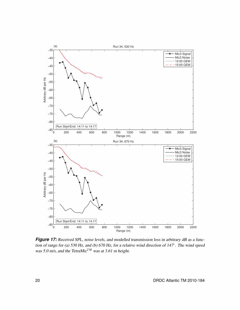
Figure 17: Received SPL, noise levels, and modelled transmission loss in arbitrary dB asa function of range for (a) 530 Hz, and (b) 670 Hz, for a relative wind directionof 147◦. The wind speed was 5.0 m/s, and the TetraMicT M was at 3.61 m height. 20
Figure 18: Received SPL, noise levels, and modelled transmission loss in arbitrary dB asa function of range for (a) 530 Hz, and (b) 670 Hz, for a relative wind directionof 175◦. The wind speed was 1.8 m/s, and the TetraMicT M was at 10.18 m height. 21
Figure 19: Received SPL and noise levels in arbitrary dB as a function of time at (a)530 Hz, and (b) 670 Hz, for the first stationary recording, taken at Point A(Figure 4). The TetraMicT M was at 10.18 m height and the wind was 6.1 m/sfrom 121◦T. . . . . . . . . . . . . . . . . . . . . . . . . . . . . . . . . . 23
xii DRDC Atlantic TM 2010-184

Figure 20: Received SPL and noise levels in arbitrary dB as a function of time at (a)530 Hz, and (b) 670 Hz, for the second stationary recording, taken at Point A(Figure 4). The TetraMicT M was at 10.18 m height and the wind was 3.5 m/sfrom 302◦T. . . . . . . . . . . . . . . . . . . . . . . . . . . . . . . . . . 24
Figure 21: Received SPL and noise levels in arbitrary dB as a function of time at (a)530 Hz, and (b) 670 Hz, for the third stationary recording, taken at Point B(Figure 4). The TetraMicT M was at 10.18 m height and the wind was 5.8 m/sfrom 321◦T. . . . . . . . . . . . . . . . . . . . . . . . . . . . . . . . . . 25
Figure 22: Received SPL (arbitrary units) for each receiver channel for four impulsivenoise events (a-d). The times of the direct and refracted arrivals are plotted asred and blue vertical lines, respectively. . . . . . . . . . . . . . . . . . . . . 26
Figure 23: The ACB, with the approximate location of the TetraMicT M indicated by a redcircle. . . . . . . . . . . . . . . . . . . . . . . . . . . . . . . . . . . . . 28
Figure B.1: Diagram of signal and noise calculation windows. The blue window is the 3-ssignal window, and the two red windows are the 3-s ‘before’ and ‘after’ noisewindows. The buffer time used in the analysis is TB = 1 s. The actual signal isplotted in blue on the bottom half of the diagram. . . . . . . . . . . . . . . . 37
Figure C.1: Received SPL, noise levels, and modelled transmission loss in arbitrary dB asa function of range for (a) 530 Hz, and (b) 670 Hz, for a relative wind directionof 7◦. The wind speed was 4.2 m/s, and the TetraMicT M was at 3.76 m height. . 41
Figure C.2: Received SPL, noise levels, and modelled transmission loss in arbitrary dB asa function of range for (a) 530 Hz, and (b) 670 Hz, for a relative wind directionof 31◦. The wind speed was 1.6 m/s, and the TetraMicT M was at 10.18 m height. 42
Figure C.3: Received SPL, noise levels, and modelled transmission loss in arbitrary dB asa function of range for (a) 530 Hz, and (b) 670 Hz, for a relative wind directionof 33◦. The wind speed was 1.9 m/s, and the TetraMicT M was at 10.18 m height. 43
Figure C.4: Received SPL, noise levels, and modelled transmission loss in arbitrary dB asa function of range for (a) 530 Hz, and (b) 670 Hz, for a relative wind directionof 73◦. The wind speed was 1.0 m/s, and the TetraMicT M was at 10.18 m height. 44
Figure C.5: Received SPL, noise levels, and modelled transmission loss in arbitrary dB asa function of range for (a) 530 Hz, and (b) 670 Hz, for a relative wind directionof 77◦. The wind speed was 1.8 m/s, and the TetraMicT M was at 3.76 m height. 45
DRDC Atlantic TM 2010-184 xiii

Figure C.6: Received SPL, noise levels, and modelled transmission loss in arbitrary dB asa function of range for (a) 530 Hz, and (b) 670 Hz, for a relative wind directionof 90◦. The wind speed was 0.9 m/s, and the TetraMicT M was at 10.18 m height. 46
Figure C.7: Received SPL, noise levels, and modelled transmission loss in arbitrary dB asa function of range for (a) 530 Hz, and (b) 670 Hz, for a relative wind directionof 94◦. The wind speed was 1.2 m/s, and the TetraMicT M was at 10.18 m height. 47
Figure C.8: Received SPL, noise levels, and modelled transmission loss in arbitrary dB asa function of range for (a) 530 Hz, and (b) 670 Hz, for a relative wind directionof 114◦. The wind speed was 0.9 m/s, and the TetraMicT M was at 10.18 m height. 48
Figure C.9: Received SPL, noise levels, and modelled transmission loss in arbitrary dB asa function of range for (a) 530 Hz, and (b) 670 Hz, for a relative wind directionof 123◦. The wind speed was 1.6 m/s, and the TetraMicT M was at 10.18 m height. 49
Figure C.10:Received SPL, noise levels, and modelled transmission loss in arbitrary dB asa function of range for (a) 530 Hz, and (b) 670 Hz, for a relative wind directionof 126◦. The wind speed was 0.7 m/s, and the TetraMicT M was at 10.18 m height. 50
Figure C.11:Received SPL, noise levels, and modelled transmission loss in arbitrary dB asa function of range for (a) 530 Hz, and (b) 670 Hz, for a relative wind directionof 139◦. The wind speed was 4.6 m/s, and the TetraMicT M was at 10.18 m height. 51
Figure C.12:Received SPL, noise levels, and modelled transmission loss in arbitrary dB asa function of range for (a) 530 Hz, and (b) 670 Hz, for a relative wind directionof 166◦. The wind speed was 1.1 m/s, and the TetraMicT M was at 10.18 m height. 52
Figure C.13:Received SPL, noise levels, and modelled transmission loss in arbitrary dB asa function of range for (a) 530 Hz, and (b) 670 Hz, for a relative wind directionof 167◦. The wind speed was 3.0 m/s, and the TetraMicT M was at 10.18 m height. 53
Figure C.14:Received SPL, noise levels, and modelled transmission loss in arbitrary dB asa function of range for (a) 530 Hz, and (b) 670 Hz, for a relative wind directionof 180◦. The wind speed was 1.6 m/s, and the TetraMicT M was at 10.18 m height. 54
xiv DRDC Atlantic TM 2010-184

1 Background
General interest in understanding atmospheric acoustic propagation over water has in-creased in recent years, driven primarily by concerns about noise from offshore wind farms.In addition, there are specic naval interests such as evaluating the performance of direc-tional acoustic hailing devices used at sea, determining potential environmental impact ofnaval gunfire exercises, and understanding the in-air acoustic footprint of maritime-basedmilitary assets. Atmospheric acoustic propagation is strongly affected by the environment,including atmospheric parameter proles (temperature, wind velocity, humidity, turbulence)and sea surface roughness. The maximum audible range in air for sound sources at sea willchange with weather conditions and sea state; unfortunately, previous experimental workin the area of atmospheric acoustic propagation over water is sparse.
In 1961, Wiener measured acoustic transmission loss in foggy conditions using a fog hornas the acoustic source [1]. Salomons demonstrated that water surface waves can stronglyaffect transmission loss in long-range over-water propagation [2]. Boue showed that spher-ical spreading (see Equation 1) is an appropriate model up to 700 m range [3]. Bolin andBoue showed that accurate predictions in shadow zones1 rely on inclusion of atmosphericturbulence in transmission loss models [4].
1.1 Acoustic transmission lossThe simplest representation of acoustic transmission loss is modelled using geometricspreading. Spherical spreading is appropriate when a source is in an unbounded, homo-geneous medium:
T L = 20log(
RR0
), (1)
in which T L is the transmission loss in decibels (dB) relative to a reference range R0 (gen-erally 1 m), and R is the range to the receiver. In practice, spherical spreading is used as afirst approximation in many applications, and is valid as long as a source is ‘far’ from anyboundaries and the medium is ‘reasonably’ homogenous.
For a source in a waveguide, that is, a medium with two parallel boundaries where the dis-tance between the boundaries is much less than the range of the measurement, cylindricalspreading is the appropriate model for the transmission loss
T L = 10log(
RR0
), (2)
where again R is the range to the receiver and R0 is the reference range.
1Shadow zones are regions where no sound rays arrive when using ray-tracing propagation models.
DRDC Atlantic TM 2010-184 1

Atmospheric absorption by dissipative processes in the atmosphere causes additional lossesbeyond the geometric spreading expected based on Equations 1 and 2, and depends stronglyon the frequency of the sound, as well as temperature and humidity of the atmosphere [5].Beyond the two simple geometric spreading models are a wide array of computationalmodels, including ray-based models, parabolic equation models, and fast field programmodels [5].
2 Experiment
An experiment was performed in July 2010 to measure the atmospheric acoustic transmis-sion loss over water, and an atmospheric acoustic propagation model was used to com-pare measured and modelled transmission loss. The experimental geometry is describedin Section 2.1, the data processing is described in Section 2.2 and Appendix B, and thepropagation model is described in Section 2.3.
2.1 Experimental geometryIn order to measure the acoustic transmission loss over water as a function of range undera variety of atmospheric conditions, an experiment was performed in the Bedford Basin,Halifax, Nova Scotia on board DRDC Atlantic’s Acoustic Calibration Barge (ACB), lo-cated at 44.6845◦N, 63.6528◦E. An overview of the experimental setup will be given here;full equipment details, including serial numbers and instrument settings, can be found inAppendix A. A schematic diagram of the experimental setup is shown in Figure 1.
The acoustic source was a dual-tone Nautilus 3500 motorcycle horn with nominal frequen-cies of 530 Hz and 670 Hz and a measured on-axis source level of 115 dB re 20 μPa at 1 m.The source was mounted aft-facing at 1.25 m height above the water on a Zodiac inflatableboat. A Sony Linear PCM Recorder was used in the Zodiac to monitor the source.
The receiver was a Core Audio TetraMicT M mounted above the barge structure at 10.18 mabove the water surface2. The TetraMicT M is a directional array of four cardiod micro-phones (Figure 2); the raw audio acquired by each microphone capsule is stored as a sepa-rate .wav file. The raw audio can then be processed in conjunction with the manufacturer-provided microphone calibration data to create four channels: one omnidirectional chan-nel and three dipoles3. A windscreen provided by the manufacturer was mounted on theTetraMicT M to minimize wind noise. The windscreen was shaped like a cylinder with ahemisphere attached to one end, and consisted of two parts: a foam core (11.4 cm high and7.9 cm in diameter) with a ‘hairy’ cover. With both the foam core and the cover in place,the windscreen was 15.0 cm high and 11.4 cm in diameter. For some runs, the TetraMicT M
2The positive x-direction in the TetraMicT M coordinate system was facing the stern of the ACB.3Dipoles are oriented along the x-, y-, and z-axes in the TetraMicT Mcoordinate system.
2 DRDC Atlantic TM 2010-184

268
305
337
38
402
436
weather station & gps[ height 9.6m ]
sample run direction
ambient noise SPL meter[ height 1.9m ]
TetraMic TM & gps [ height 10.2m ] ADCP
source [ height 1.25m ]
uy
ux
20 m
Figure 1: Experimental setup. Zodiac runs were done toward and away from the ACB (greyrectangle) in various directions. Coordinate system for wind velocity is indicated at top right by ux
and uy. Water depths and contours (m, dm) are indicated in blue.
was moved to a lower position (3.61 m to 3.76 m above the water surface) because the windnoise was causing clipping4 on the recording. The TetraMicT M microphone directions areshown schematically in Figure 3.
Three types of recordings were made with the TetraMicT M: moving source, stationarysource, and (improvised) impulsive sources. In all cases, a series of three ‘timing’ blasts(short, quick blasts of the horn) were sounded when the Zodiac was near the ACB at thebeginning and end of each run to synchronize the audio tracks with each other and with theGPS. The GPS time at the start of the third timing blast was noted in the log book, and thetwo audio tracks were synchronized by calculating their cross-correlation, as described inmore detail in Appendix B.1.
For the moving source recordings, the Zodiac was driven away from and towards the ACBat speeds of 4 to 8 knots to distances of up to 3 km. One person on the Zodiac was assignedto sound the horn for specified lengths of time at specified intervals that were timed usinga watch, and the Zodiac was turned around for the inward-bound run when the horn wasno longer audible on board the ACB. There were a total of 20 moving-source runs duringwhich the horn was sounded every 20 s for 5 s; for three runs, the horn was sounded every10 s for as short a blast as possible (in practice, about 0.3 s).
4The signal exceeded the maximum analog-to-digital (A/D) range available.
DRDC Atlantic TM 2010-184 3

Figure 2: The receiver used in the experiments: (a) the TetraMicT M, (b) with foam windscreen inplace, (c) with ‘hairy’ wind screen in place over the foam.
N1
2 3
4
Barge (side view)
1 2
3 4
Barge (top view)
(a) (b)
NW
Figure 3: Microphone directions. Channels are numbered as indicated on the diagram (not toscale).
For the stationary source recordings, the horn was sounded every 20 s for 5 s for a total offive minutes, followed by as-short-as-possible blasts every 10 s for a total of five minutes.For the first two stationary recordings, the Zodiac was tied to a buoy at 286 m range fromthe ACB (Point A in Figure 4). For the third stationary recording, the Zodiac was tied tothe ACB with a rope and drifted downwind until it came to a stop at a distance of 119 mfrom the ACB, and the horn blasts began once the Zodiac had stabilized in heading andrange (Point B in Figure 4).
For impulsive sources, recordings were made by popping balloons while the Zodiac driftedfrom a range of 95 m to 121 m (Point C in Figure 4).
The ambient noise level at the ACB and horn source level were measured several times
4 DRDC Atlantic TM 2010-184

Figure 4: Locations for the Zodiac, relative to the ACB (green marker at 44.6845◦N, 63.6528◦W)for the first two stationary recordings (Point A) and the third stationary recording (Point B). Point Cis the location of the impulsive source, described in Section 3.4. The ADCP location (44.6847◦N,63.6517◦W) is indicated with a blue marker. Scale is at bottom left.
Figure 5: Sample Zodiac GPS track (green line). The ACB location at 44.6845◦N, 63.6528◦W isindicated with a green marker. Scale is at bottom left.
each day with a Bruel & Kjær (B & K) sound pressure level (SPL) meter. Directional oceansurface wave spectra were measured using a Teledyne RD Instruments Acoustic DopplerCurrent Profiler (ADCP) operating at 300 kHz. GlobalSat global positioning system (GPS)antennas were mounted on the east and west corners of the ACB to monitor barge headingand position. A handheld GPS receiver (Garmin Oregon 55T) was used on the Zodiac torecord its position during the runs (a sample track is shown in Figure 5).
Point measurements of temperature, wind velocity, humidity, and air pressure were madeat the ACB at 9.6 m height using a Vaisala WXT520 meteorological station. The meteoro-logical station was aligned with its ‘north’ direction parallel to the ACB bow-stern axis andthe wind directions were corrected in the post-processing stage using the measured ACBheading. Vaisala Radiosondes were launched from Canadian Forces Base (CFB) Halifax(6 km SE of the ACB) on each day at 0930 and 1230 local time to record atmospheric
DRDC Atlantic TM 2010-184 5

parameter profiles. Parameter profiles from Environment Canada’s Global EnvironmentalMultiscale (GEM) model [6, 7, 8] were available at 0900, 1200, and 1500 local time eachday.
2.2 Data processingA general outline of the data processing steps will be given in this section, while the detailsof the data processing can be found in Appendix B. Data processing consisted of severalsteps that were implemented using MATLAB: synchronizing the files, identifying hornblasts, and calculating the received SPL.
The audio files fell into two groups: the stereo ‘monitor’ tracks recorded using the Sonyrecorder on the Zodiac, and the four mono ‘receiver’ tracks recorded using the TetraMicT M
mounted on the ACB. Before the automated steps of the data processing could be per-formed, the data files were listened to and examined using the spectrogram function inAudacity (audio mixing software). The left channel of the stereo monitor track was usedto determine blast start times and file synchronization. The start time of the third ‘timingblast’ for each monitor and receiver file was noted to the nearest second, relative to thebeginning of the file. In addition, the time of the first ‘data blast’ and the time after whichthere were no more data blasts were noted for each monitor file. The times of the firstand last data blasts and the third timing blast were used as inputs to the automatic blastidentification algorithm described below and in Appendix B.
The cross-correlation of the horn timing blasts between the monitor and receiver files wasused to accurately determine the lag between files (Appendix B.1). The range to the Zodiacat the mid-point of each blast was calculated using the ACB and Zodiac GPS coordinates(Appendix B.2). Start and end times for each horn blast were detected using the monitortrack recorded by the Sony recorder on the Zodiac (Appendix B.3). The received SPL wascalculated from the receiver files using the detected blast time from the monitor track andtaking into account the delay as the sound travelled to the receiver5, along with a buffer toavoid horn start and end effects (Appendix B.4). Noise levels were estimated 2 s before andafter each horn blast and interpolated to obtain the noise level during each blast (AppendixB.5).
In order to calculate the received SPL, the frequency band chosen had to be wide enoughto take into account the horn frequency instability and the Doppler shift resulting from therelative motion of the Zodiac and the ACB. The horn frequency varied between 525 Hzand 544 Hz for the nominal 530 Hz tone, and 666 Hz and 688 Hz for the nominal 670 Hztone. The maximum Doppler shift at 8 knots and 688 Hz is 8 Hz. Therefore, the receivedSPL was averaged across a frequency band wide enough to account for Doppler shift,horn frequency instability, and a small additional buffer (525± 25 Hz and 677± 25 Hz).
5The sound speed was calculated using the mean measured air temperature for the run.
6 DRDC Atlantic TM 2010-184

The same two frequency bands were used to estimate the noise level during each blast(Appendix B.5).
2.3 ModellingThe Sensor Performance Evaluator for Battlefield Environments (SPEBE) [9] is an in-air acoustic propagation and sensor performance model that can compute acoustic trans-mission loss given inputs for terrain, ground type, meteorology, and source and receiverspecficiations. A set of modelling runs was undertaken in order to compare the measuredtransmission loss with that obtained by using SPEBE in conjunction with both measuredand modelled atmospheric parameter profiles.
The terrain was input from a Digital Terrain Elevation Database [10], using a 2-km by 2-km square centred on the barge microphone location at 44.6845◦N, 63.6528◦W. The groundtype in SPEBE is range-independent; therefore, an infinite impedance water surface wasused, with a root-mean-square (RMS) roughness height of 0.2 m. Over a water surface, theroughness height implemented in SPEBE affects only the atmospheric parameter profilesand is not used for calculating reflection coefficients; preliminary tests suggest that themodel results were not sensitive to the choice of roughness height. The source heightwas 1.25 m, and the receiver height was 10.4 m, 3.76 m, or 3.61 m, corresponding to thereceiver height for the run being modelled. Transmission loss was modelled at 530 Hz forall the runs and 670 Hz for some of the runs, using the fast field program model includedin SPEBE [11, 12].
MetOc Halifax provided profiles of temperature, wind velocity (i.e., speed and direction),relative humidity, and atmospheric pressure. Profiles were obtained from radiosondeslaunched at CFB Halifax and from Environment Canada’s GEM weather model. The mod-elled profiles were adjusted using measured surface data from the North Magazine Jettyon the NE shore of the Bedford Basin (44.7067◦N, 63.6333◦W) except for the sea levelpressure, which was obtained from the Shearwater Airport (44.6333◦N, 63.5000◦W).
SPEBE can accept a variety of formats for meteorological inputs. For the model runspresented here, parameters were provided as a function of height in metres: temperature Tin degrees Celsius; the wind speeds ux and uy in m/s in the east-west (x) and north-south (y)directions (see Figure 1 for convention); and the dimensionless specific humidity q. Thespecific humidity was computed from the relative humidity U , pressure p (in millibars),and temperature T using [13, 14]
q =r
1+ r=
rwU1+ rwU
, (3)
where
rw = ε(
ew(T )p− ew(T )
)= 0.62197
(ew(T )
p− ew(T )
), (4)
DRDC Atlantic TM 2010-184 7

340 345 3500
50
100
150
200
250
300
350
400
ceff
(m/s)
Hei
ght (
m)
20−Jul−2010 +x−direction
(a)
GEM (12:00)Sonde (12:29)
340 345 3500
50
100
150
200
250
300
350
400
ceff
(m/s)
Hei
ght (
m)
20−Jul−2010 −x−direction
(b)
GEM (12:00)Sonde (12:29)
340 345 3500
50
100
150
200
250
300
350
400
ceff
(m/s)
Hei
ght (
m)
20−Jul−2010 +y−direction
(c)
GEM (12:00)Sonde (12:29)
340 345 3500
50
100
150
200
250
300
350
400
ceff
(m/s)
Hei
ght (
m)
20−Jul−2010 −y−direction
(d)
GEM (12:00)Sonde (12:29)
Figure 6: Effective sound speed ce f f as a function of height for (a) positive x-direction, (b) negativex-direction, (c) positive y-direction, and (d) negative y-direction, for measured (radiosonde) andmodelled (GEM) atmospheric parameter profiles.
and
ew(T ) = 6.112exp(
17.67TT +243.5
). (5)
Figure 6 is a plot of the effective sound speed as a function of height in the atmospherece f f (z) along the positive and negative x-directions for measured (radiosonde) and mod-elled (GEM) atmospheric parameter profiles. The sound speed as a function of height wasfirst calculated from the temperature profile T (z):
c(z) = c0
√T (z)T0
(6)
where T (z) is measured in Kelvin, c0 = 331 m/s, and T0 = 273K. (Equation 6 is strictlyvalid only for dry air, but the correction for a nonzero relative humidity will increase thesound speed by no more than 0.3% [5]). The effective sound speed as a function of heightce f f (z) plotted in Figure 6 is calculated to first order by summing the sound speed profilec(z) for still air and the component u(z) of the wind velocity in the direction of interest [5]:
ce f f (z) = c(z)+u(z) (7)
8 DRDC Atlantic TM 2010-184

The sign of the sound speed gradient ∂ce f f /∂z determines whether the atmosphere isdownward-refracting (∂ce f f /∂z> 0) or upward-refracting (∂ce f f /∂z< 0) [5]. In downward-refracting conditions, there is a ‘turning point’ for acoustic rays at some height in the at-mosphere, so that in a ray model, rays interact repeatedly with the ground surface. Theresult is that at some ranges there are many possible ray paths and high received SPL, andat other intermediate ranges there are fewer or no rays and correspondingly lower receivedSPL. In upward-refracting conditions, rays are refracted away from the ground, and thereis a region where no rays arrive called the ‘shadow zone’; in practice, sound penetratesthe shadow zone through diffraction and turbulent scattering [5]. For the profiles ce f f (z)along the positive and negative x-directions (Figures 6a and b), the radiosonde profile (redline) in Figure 6b has a generally positive gradient over the whole profile and is there-fore downward-refracting; the other three profiles are upward-refracting. For the profilesce f f (z) along the positive and negative y-directions (Figure 6c and d), the lower 150 m ofthe radiosonde profiles is downward-refracting, while the entire GEM profile is upward-refracting.
Atmospheric turbulence can also have an effect on acoustic transmission loss, and severaloptions for modelling atmospheric turbulence are available in SPEBE [15]. The turbulencemodels selected use a combination of the Mann rapid distortion theory model [16] to gen-erate velocity fluctuations caused by wind shear, the Hunt/Graham/Wilson modification[17] of the von Karman turbulence model to generate turbulence caused by buoyancy, andan isotropic von Karman model [18] to generate temperature fluctuations. The parame-ters used for model input were an inversion layer height zi = 1000 m, a friction velocityu∗ = 0.1+ u0/20 , and a surface-layer temperature scale T∗ = −0.3+ u0/50, where u0 isthe surface wind speed. These correspond in general to SPEBE’s sunny day profile case,and should therefore be reasonably representative of the conditions on July 19-21 and July23. The weather on July 22 was cloudy with some rain.
Figure 8 is a sample of transmission loss calculated using SPEBE for a receiver at thecentre of the image (indicated by �) and a source at any position within the image, usingthe measured atmospheric parameter profiles from 09:29 on 23 Jul 2010. The anisotropyin the modelled transmission loss to the west of the ACB are likely due to a combinationof atmospheric refraction and the local topography (there is land to the west of the ACB).Transmission loss along the black line representing a Zodiac track in Figure 8 connectingthe receiver with a source position (•) is plotted as a function of range in Figure 9.
3 Results and discussion
Representative model results for different atmospheric inputs and source frequencies arediscussed in Section 3.1. The three types of recordings (moving source, stationary source,and impulsive source) were acquired to investigate different effects. The moving-sourcerecordings (Section 3.2) were used to examine the effects on received SPL of source-
DRDC Atlantic TM 2010-184 9

335 340 345 3500
50
100
150
200
250
300
350
400
ceff
(m/s)
Hei
ght (
m)
23−Jul−2010 +x−direction(a)
335 340 345 3500
50
100
150
200
250
300
350
400
ceff
(m/s)
Hei
ght (
m)
23−Jul−2010 −x−direction(b)
335 340 345 3500
50
100
150
200
250
300
350
400
ceff
(m/s)
Hei
ght (
m)
23−Jul−2010 +y−direction(c)
335 340 345 3500
50
100
150
200
250
300
350
400
ceff
(m/s)
Hei
ght (
m)
23−Jul−2010 −y−direction(d)
Figure 7: Effective sound speed ce f f as a function of height for (a) positive x-direction, (b) neg-ative x-direction, (c) positive y-direction, and (d) negative y-direction, for measured (radiosonde)atmospheric parameter profiles. The resulting transmission loss calculated by SPEBE is plotted inFigure 8.
receiver range, microphone height, and wind speed. The stationary recordings were usedto attempt to quantify the time variability in received SPL by removing the range depen-dence (Section 3.3). A first attempt at acquiring impulsive source recordings in order todetermine the effects, if any, of multipath propagation, is described in Section 3.4.
3.1 Overview of model resultsModel runs were performed at 530 Hz for all the available atmospheric parameter pro-files. However, in order to determine whether the transmission loss differs between the twosource frequencies of 530 Hz and 670 Hz, the SPEBE model was run at both frequenciesfor two sets of atmospheric conditions. Figure 10 is a plot of the modelled transmissionloss as a function of latitude and longitude for 530 Hz and 670 Hz using a measured at-mospheric profile (Figures 10a and b, respectively), and for 530 Hz and 670 Hz using amodelled atmospheric profile (Figures 10c and d, respectively). For a given atmosphericparameter profile, the plots at the two frequencies look qualitatively similar with down-ward refraction causing alternating rings of lower and higher transmission loss; however,the detailed shape of the transmission loss pattern differs between frequencies.
The transmission loss along the black line in Figure 10 is extracted and plotted as a functionof range from the ACB in Figure 11. There are significant differences in transmission lossfor the two frequencies, especially for the case in Figure 11a. The downward-refracting
10 DRDC Atlantic TM 2010-184

00
0
0
10
10
10
20
20
20
30
30
30
4040
40
40
40
50
50
50
60
60
60
70
70
80
Longitude
Latit
ude
SPEBE output, 530 Hz, radiosonde launch, 09:29 on 23 Jul 2010
−63.67 −63.66 −63.65 −63.64 −63.63
44.67
44.675
44.68
44.685
44.69
44.695
44.7
Tra
nsm
issi
on lo
ss (
dB)
−90
−80
−70
−60
−50
−40
−30
Figure 8: Sample SPEBE output: transmission loss (dB) as a function of latitude and longitude,for a receiver at the centre of the image (�) and a source at any point in the image, with topographiccontours (m) shown as solid black lines. The atmospheric parameter profiles used are shown inFigure 7. The transmission loss along the black dashed line for a source at the black circle (•) isinterpolated and plotted as a function of range in Figure 9.
0 200 400 600 800 1000 1200 1400 1600 1800−80
−70
−60
−50
−40
−30
−20
Range (m)
Tra
nsm
issi
on lo
ss (
dB r
e 1
m)
Figure 9: Interpolation of transmission loss from sample SPEBE output shown in Figure 8.
DRDC Atlantic TM 2010-184 11

Longitude
Latit
ude
530 Hz, 12:32 on Jul 22, radiosonde
(a)
−63.67 −63.66 −63.65 −63.64 −63.63
44.67
44.675
44.68
44.685
44.69
44.695
44.7
Tra
nsm
issi
on lo
ss (
dB)
−100
−90
−80
−70
−60
−50
−40
−30
Longitude
Latit
ude
670 Hz, 12:32 on Jul 22, radiosonde
(b)
−63.67 −63.66 −63.65 −63.64 −63.63
44.67
44.675
44.68
44.685
44.69
44.695
44.7
Tra
nsm
issi
on lo
ss (
dB)
−100
−90
−80
−70
−60
−50
−40
−30
Longitude
Latit
ude
530 Hz, 12:00 on Jul 23, GEM
(c)
−63.67 −63.66 −63.65 −63.64 −63.63
44.67
44.675
44.68
44.685
44.69
44.695
44.7
Tra
nsm
issi
on lo
ss (
dB)
−100
−90
−80
−70
−60
−50
−40
−30
Longitude
Latit
ude
670 Hz, 12:00 on Jul 23, GEM
(d)
−63.67 −63.66 −63.65 −63.64 −63.63
44.67
44.675
44.68
44.685
44.69
44.695
44.7
Tra
nsm
issi
on lo
ss (
dB)
−100
−90
−80
−70
−60
−50
−40
−30
Figure 10: Modelled transmission loss centred on the ACB (white dot) for (a) 530 Hz, radiosondedata, (b) and 670 Hz, radiosonde data, (c) 530 Hz, GEM output, (d) 670 Hz, GEM output, withdates and times as indicated on the plots. The black line indicates the profile extracted and plottedin Figure 11.
atmosphere results in local minima in transmission loss at different ranges for each fre-quency: 600 m, 1200 m, and 1800 m at 530 Hz, and 700 m and 1450 m at 670 Hz. Thedifferences in transmission loss between the two frequencies in Figure 11b are generallyless than 5 dB.
3.2 Moving-source recordingsReceived SPL was calculated for the 20 moving-source runs for distances up to 2.2 km(the maximum audible range). Of the meteorological parameters that affect atmosphericacoustic propagation, the wind velocity (i.e., direction and speed) relative to the source-receiver direction most strongly affects the received SPL. In general, wind velocity varieswith height in the atmosphere (e.g., Figures 6 and 7) and the SPEBE model takes thefull vertical wind profile into account. In order to organize the datasets, a representativerelative wind direction was calculated using the average wind velocity measured at theACB during a given run. Using the source-to-receiver direction as a reference for the wind
12 DRDC Atlantic TM 2010-184

0 200 400 600 800 1000 1200 1400 1600 1800 2000−90
−80
−70
−60
−50
−40
−30
−20
Range (m)T
rans
mis
sion
loss
(dB
)
12:32 on Jul 22, radiosonde
(a)
530 Hz670 Hz
0 200 400 600 800 1000 1200 1400 1600 1800 2000−90
−80
−70
−60
−50
−40
−30
−20
Range (m)
Tra
nsm
issi
on lo
ss (
dB)
12:00 on Jul 23, GEM
(b)
530 Hz670 Hz
Figure 11: Modelled transmission loss along the black line in Figure 10 (due east of the ACB) for530 Hz (blue) and 670 Hz (red), for (a) radiosonde data and (b) GEM output.
velocity vector, the ‘downwind’ wind direction is 0◦, the ‘crosswind’ direction is 90◦, andthe ‘upwind’ direction is 180◦. Table C.1 in Appendix C.1 is a summary of runs and relativewind velocity for all of the moving-source runs. Wind speed varied from 0.9 m/s to 5.0 m/s,and the relative wind direction varied from 7◦(nearly downwind) to 180◦(upwind).
Figure 12 is a plot of received SPL as a function of range for all four raw TetraMicT M chan-nels and the 530-Hz nominal horn tone. Generally, the highest received level is observedon the microphones most closely aligned with the run direction (microphones 3 and 4). Forease of interpretation, the remaining plots of received SPL as a function of range will onlyinclude the microphone measuring the highest received level.
The moving-source recordings allowed for examination of the range dependence of thereceived SPL (Section 3.2.1), the dependence of received SPL on receiver height (Section3.2.2), and the effect of changes in wind speed (Section 3.2.3).
3.2.1 Range dependence of received SPL
Figure 13 is a plot of received SPL as a function of range for a downwind run for the 530-Hz and 670-Hz nominal horn tones (Figures 13a and b, respectively). For the run in Figure13, the receiver had been lowered to a height of 3.76 m above the water, and mountedon the east corner of the barge deck, because wind noise had been causing clipping in itsoriginal position. The maximum range at which the horn is detectable above the noisefloor is 1800 m. The higher-SPL ‘spikes’ at 1200 m and 1450 m (Figure 13) may be dueto acoustic convergence zones caused by a downward-refracting atmosphere. Since the
DRDC Atlantic TM 2010-184 13

0 200 400 600 800 1000 1200 1400 1600 1800 2000 2200−85
−80
−75
−70
−65
−60
−55
−50
−45
−40
−35
Range (m)
Arb
itrar
y dB
per
Hz
Run 27, 530 Hz
Run Start/End: 13:08 to 13:22
Mic1 SignalMic1 NoiseMic2 SignalMic2 NoiseMic3 SignalMic3 NoiseMic4 SignalMic4 Noise12:00 GEM12:32 Sonde15:00 GEM
Figure 12: Received SPL, noise levels, and modelled transmission loss in arbitrary dB at 530 Hzas a function of range for a relative wind direction of 8◦(downwind). The wind speed was 3.4 m/s,and the TetraMicT M was at 3.76 m height.
absolute calibration of the receiver is not known, the modelled transmission loss can onlybe compared with measurements in a qualitative way. A similar pattern of maxima andminima can be seen in two of the SPEBE results (using 12:00 GEM and 12:32 radiosondeprofiles), although the maxima and minima occur at different ranges than in the measure-ments. In contrast, the SPEBE output using the 15:00 GEM profile drops off smoothly withincreasing range to a range of 1500 m, then suddnely drops by 10dB.
Figure 14 is a plot of received SPL as a function of range for a crosswind run. The receiverwas at a height of 3.76 m on the east corner of the ACB. At 700 m range, the received SPLdrops suddenly by 15 dB and remains low, but the horn is still detectable above the noisefloor until the end of the run at 1300 m range (Figure 14). None of the modelled lines fortransmission loss agree very well with the measurements: the GEM output does not showthe sharp drop-off at 700 m range, and the radiosonde output shows maxima and minimathat are not evident in the data.
Figure 15 is a plot of received SPL as a function of range for an upwind run, with theTetraMicT M at a height of 10.18 m. The received SPL first drops below the noise floor at500 m range, is faintly audible until 600 m range, and then drops below the noise flooragain. The modelled SPL using the radiosonde profile shows a steep drop-off between100 m and 600 m range that is similar to the measurements, whereas the model resultsusing the GEM profiles show an essentially linear decrease in received level with range.
14 DRDC Atlantic TM 2010-184

0 200 400 600 800 1000 1200 1400 1600 1800 2000 2200−85
−80
−75
−70
−65
−60
−55
−50
−45
−40
−35
Range (m)
Arb
itrar
y dB
per
Hz
Run Start/End: 13:08 to 13:22
Run 27, 530 Hz(a)
Mic3 SignalMic3 Noise12:00 GEM12:32 Sonde15:00 GEM
0 200 400 600 800 1000 1200 1400 1600 1800 2000 2200−85
−80
−75
−70
−65
−60
−55
−50
−45
−40
−35
Range (m)
Arb
itrar
y dB
per
Hz
Run Start/End: 13:08 to 13:22
Run 27, 670 Hz(b)
Mic3 SignalMic3 Noise12:00 GEM12:32 Sonde15:00 GEM
Figure 13: Received SPL, noise levels, and modelled transmission loss in arbitrary dB as a func-tion of range for (a) 530 Hz, and (b) 670 Hz, for a relative wind direction of 8◦(downwind). Thewind speed was 3.4 m/s, and the TetraMicT M was at 3.76 m height.
DRDC Atlantic TM 2010-184 15

0 200 400 600 800 1000 1200 1400 1600 1800 2000 2200−85
−80
−75
−70
−65
−60
−55
−50
−45
−40
−35
Range (m)
Arb
itrar
y dB
per
Hz
Run Start/End: 13:38 to 13:49
Run 28, 530 Hz(a)
Mic4 SignalMic4 Noise12:00 GEM12:32 Sonde15:00 GEM
0 200 400 600 800 1000 1200 1400 1600 1800 2000 2200−85
−80
−75
−70
−65
−60
−55
−50
−45
−40
−35
Range (m)
Arb
itrar
y dB
per
Hz
Run Start/End: 13:38 to 13:49
Run 28, 670 Hz(b)
Mic4 SignalMic4 Noise12:00 GEM12:32 Sonde15:00 GEM
Figure 14: Received SPL, noise levels, and modelled transmission loss in arbitrary dB as a func-tion of range for (a) 530 Hz, and (b) 670 Hz, for a relative wind direction of 95◦(crosswind). Thewind speed was 2.7 m/s, and the TetraMicT M was at 3.76 m height.
16 DRDC Atlantic TM 2010-184

0 200 400 600 800 1000 1200 1400 1600 1800 2000 2200−85
−80
−75
−70
−65
−60
−55
−50
−45
−40
−35
Range (m)
Arb
itrar
y dB
per
Hz
Run Start/End: 13:23 to 13:31
Run 10, 530 Hz(a)
Mic3 SignalMic3 Noise12:00 GEM12:30 Sonde15:00 GEM
0 200 400 600 800 1000 1200 1400 1600 1800 2000 2200−85
−80
−75
−70
−65
−60
−55
−50
−45
−40
−35
Range (m)
Arb
itrar
y dB
per
Hz
Run Start/End: 13:23 to 13:31
Run 10, 670 Hz(b)
Mic3 SignalMic3 Noise12:00 GEM12:30 Sonde15:00 GEM
Figure 15: Received SPL, noise levels, and modelled transmission loss in arbitrary dB as a func-tion of range for (a) 530 Hz, and (b) 670 Hz, for a relative wind direction of 177◦(upwind). Thewind speed was 3.3 m/s, and the TetraMicT M was at 10.18 m height.
DRDC Atlantic TM 2010-184 17

3.2.2 Microphone height
The effect of microphone height can be determined by comparing Figures 16 and 17, whichwere recorded with the receiver at 10.18 m and 3.61 m height, respectively. The tworecordings were made on the same day (23 July), with comparable wind speeds (4.9 m/sand 5.0 m/s, respectively) and in similar directions (source-to-receiver bearings of 274◦and 316◦ true, respectively). The greatest effect of height is on the noise level, which isbetween -65 dB and -70 dB for the 10.18 m receiver height, and between -70 dB and -80dB for the 3.61 m height. Auditory inspection of the recorded tracks reveals that there aretwo main sources of noise on the recordings for 10.18 m height: severe radio interference,and wind noise. For the recordings at 3.61 m height, the main source of noise is the soundof water lapping against the side of the ACB. As a result, the 3.61 m height recording ismuch ‘cleaner’.
3.2.3 Wind speed
Most of the wind speeds experienced during the experiment were low compared to whatmight be experienced on the open ocean: the maximum wind speed during the experimentwas 5.0 m/s (10 knots). Within the dataset there are some pairs of runs with ‘low’ (< 2 m/s)and ‘high’ (> 2 m/s) wind speeds and comparable relative wind directions. Figures 15 and18 are plots of received SPL as a function of range with a wind speed of 3.3 m/s and1.8 m/s (relative directions of 177◦and 175◦), respectively. In both cases, the receiver wasat 10.18 m height. The maximum range for which the horn was detectable above the noisewas 600 m for the 3.3 m/s wind speed, compared with 1000 m for the 1.8 m/s wind speed,suggesting that even at low overall wind speeds, a slight increase in wind velocity can resultin a significant difference in maximum detectable range.
3.3 Stationary recordingsIn order to quantify the time variability in received SPL, three recordings were made withthe source stationary; however, each recording was plagued by a different set of problemsand none resulted in data that were entirely satisfactory. The first two stationary recordingstook place while the Zodiac with the source was tied to a buoy 286 m away from the ACB(Point A in Figure 4), and the third recording took place with the Zodiac tied to the ACBwith a rope at 119 m range (Point B in Figure 4). The specific details of the stationarymeasurements as described in the following paragraphs illustrate several of the difficultiesof making acoustic transmission loss measurements over water from two moving platformsin the middle of a city.
Figure 19 is a plot of the received SPL as a function of time for the first stationary recording,made on 22 July while the Zodiac was at Point A (Figure 4). Received SPL measurementsthat experienced clipping are plotted as hollow plot symbols, while unclipped data are
18 DRDC Atlantic TM 2010-184

0 200 400 600 800 1000 1200 1400 1600 1800 2000 2200−85
−80
−75
−70
−65
−60
−55
−50
−45
−40
−35
Range (m)
Arb
itrar
y dB
per
Hz
Run Start/End: 11:35 to 11:48
Run 32, 530 Hz(a)
Mic4 SignalMic4 Noise09:00 GEM09:29 Sonde12:00 GEM
0 200 400 600 800 1000 1200 1400 1600 1800 2000 2200−85
−80
−75
−70
−65
−60
−55
−50
−45
−40
−35
Range (m)
Arb
itrar
y dB
per
Hz
Run Start/End: 11:35 to 11:48
Run 32, 670 Hz(b)
Mic4 SignalMic4 Noise09:00 GEM09:29 Sonde12:00 GEM
Figure 16: Received SPL, noise levels, and modelled transmission loss in arbitrary dB as a func-tion of range for (a) 530 Hz, and (b) 670 Hz, for a relative wind direction of 140◦. The wind speedwas 4.9 m/s, and the TetraMicT M was at 10.18 m height.
DRDC Atlantic TM 2010-184 19
0 200 400 600 800 1000 1200 1400 1600 1800 2000 2200−85
−80
−75
−70
−65
−60
−55
−50
−45
−40
−35
Range (m)
Arb
itrar
y dB
per
Hz
Run Start/End: 14:11 to 14:17
Run 34, 530 Hz(a)
Mic3 SignalMic3 Noise12:00 GEM15:00 GEM
0 200 400 600 800 1000 1200 1400 1600 1800 2000 2200−85
−80
−75
−70
−65
−60
−55
−50
−45
−40
−35
Range (m)
Arb
itrar
y dB
per
Hz
Run Start/End: 14:11 to 14:17
Run 34, 670 Hz(b)
Mic3 SignalMic3 Noise12:00 GEM15:00 GEM
Figure 17: Received SPL, noise levels, and modelled transmission loss in arbitrary dB as a func-tion of range for (a) 530 Hz, and (b) 670 Hz, for a relative wind direction of 147◦. The wind speedwas 5.0 m/s, and the TetraMicT M was at 3.61 m height.
20 DRDC Atlantic TM 2010-184

0 200 400 600 800 1000 1200 1400 1600 1800 2000 2200−85
−80
−75
−70
−65
−60
−55
−50
−45
−40
−35
Range (m)
Arb
itrar
y dB
per
Hz
Run Start/End: 12:45 to 12:55
Run 19, 530 Hz(a)
Mic3 SignalMic3 Noise12:00 GEM12:39 Sonde15:00 GEM
0 200 400 600 800 1000 1200 1400 1600 1800 2000 2200−85
−80
−75
−70
−65
−60
−55
−50
−45
−40
−35
Range (m)
Arb
itrar
y dB
per
Hz
Run Start/End: 12:45 to 12:55
Run 19, 670 Hz(b)
Mic3 SignalMic3 Noise12:00 GEM12:39 Sonde15:00 GEM
Figure 18: Received SPL, noise levels, and modelled transmission loss in arbitrary dB as a func-tion of range for (a) 530 Hz, and (b) 670 Hz, for a relative wind direction of 175◦. The wind speedwas 1.8 m/s, and the TetraMicT M was at 10.18 m height.
DRDC Atlantic TM 2010-184 21

plotted as filled symbols. The recording shown in Figure 19 suffered from two significantsources of noise: clipping, due to the wind speed of 6.1 m/s; and a resonant ‘whistling’noise that originated from a pipe attached to the structure of the ACB. The pipe had a seriesof holes in the southeast-facing direction, so that when the wind blew from the southeast(as it did during the dataset shown in Figure 19), the pipe acted like a flute and producedtones in the range of 400-850 Hz that were comparable to or greater in intensity than thereceived level from the horn.
The stationary recording was repeated on 23 July with a different wind direction, in anattempt to overcome the problems encountered in the first recording. Figure 20 is a plot ofthe received SPL as a function of time for the second stationary recording, made while theZodiac was tied to the same buoy (Point A in Figure 4). However, the wind blew the Zodiacto the far side of the buoy (relative to the ACB) during the recording. The direct line-of-sight to the ACB was blocked by the buoy and the Zodiac was unable to maintain a constantheading. The horn was not omnidirectional; therefore, the combination of the movingZodiac and the buoy blocking the direct line-of-sight resulted in unusable measurements.
The third stationary recording was made on 23 July with the Zodiac and source at Point B.The recording was started once the Zodiac came to a stop with a stable heading. Figure21 is a plot of received SPL as a function of time for the third recording. However, noisewas again a problem: the wind speed was relatively high (5.8 m/s), resulting in substantialclipping as indicated by the hollow plot symbols in Figure 21; and there were audiblecommercial radio signals being picked up on the recording; therefore, it is not clear thatthe data are reliable.
3.4 Impulsive sourcesIn order to attempt to separate multipath arrivals, latex balloons were used as impulsivesound sources. The Zodiac with the balloons was drifting at 128 m range from the ACB, atPoint C in Figure 4, and the balloons were popped at intervals of 15-19 s at a height of 2 mabove the water surface.
Figure 22 is a plot of received SPL for each TetraMicT M channel as a function of time foreach of four impulsive source events. As shown schematically in Figure 3, Microphones3 and 4 were approximately facing the Zodiac, while Microphones 1 and 2 were facingaway from the Zodiac; Microphones 1 and 4 were facing upward while Microphones 2and 3 were facing downward. As a result, the direct-path arrival is barely detectable onMicrophone 1; however, Microphone 1 measures the highest level for a multipath arrivalapproximately 20 ms after the direct-path arrival. The time difference between the twoarrivals for each impulsive source event is shown in Table 1, and is quite stable with anaverage value of 23.4 ms.
22 DRDC Atlantic TM 2010-184

−50 0 50 100 150 200 250 300 350 400−85
−80
−75
−70
−65
−60
−55
−50
−45
−40
−35
Time since the start of the first blast (s)
Arb
itrar
y dB
per
Hz
Run 25, 530 Hz, received level (•), clipped received level (°), noise (−)
Run Start/End: 11:29 to 11:34
(a)
Mic1Mic2Mic3Mic4
−50 0 50 100 150 200 250 300 350 400−85
−80
−75
−70
−65
−60
−55
−50
−45
−40
−35
Time since the start of the first blast (s)
Arb
itrar
y dB
per
Hz
Run 25, 670 Hz, received level (•), clipped received level (°), noise (−)
Run Start/End: 11:29 to 11:34
(b)
Mic1Mic2Mic3Mic4
Figure 19: Received SPL and noise levels in arbitrary dB as a function of time at (a) 530 Hz, and(b) 670 Hz, for the first stationary recording, taken at Point A (Figure 4). The TetraMicT M was at10.18 m height and the wind was 6.1 m/s from 121◦T.
DRDC Atlantic TM 2010-184 23

−50 0 50 100 150 200 250 300 350 400−85
−80
−75
−70
−65
−60
−55
−50
−45
−40
−35
Time since the start of the first blast (s)
Arb
itrar
y dB
per
Hz
Run 30, 530 Hz, received level (•), clipped received level (°), noise (−)
Run Start/End: 11:00 to 11:05
(a)
Mic1Mic2Mic3Mic4
−50 0 50 100 150 200 250 300 350 400−85
−80
−75
−70
−65
−60
−55
−50
−45
−40
−35
Time since the start of the first blast (s)
Arb
itrar
y dB
per
Hz
Run 30, 670 Hz, received level (•), clipped received level (°), noise (−)
Run Start/End: 11:00 to 11:05
(b)
Mic1Mic2Mic3Mic4
Figure 20: Received SPL and noise levels in arbitrary dB as a function of time at (a) 530 Hz, and(b) 670 Hz, for the second stationary recording, taken at Point A (Figure 4). The TetraMicT M wasat 10.18 m height and the wind was 3.5 m/s from 302◦T.
24 DRDC Atlantic TM 2010-184

−50 0 50 100 150 200 250 300 350 400−85
−80
−75
−70
−65
−60
−55
−50
−45
−40
−35
Time since the start of the first blast (s)
Arb
itrar
y dB
per
Hz
Run 33, 530 Hz, received level (•), clipped received level (°), noise (−)
Run Start/End: 12:54 to 12:59
(a)
Mic1Mic2Mic3Mic4
−50 0 50 100 150 200 250 300 350 400−85
−80
−75
−70
−65
−60
−55
−50
−45
−40
−35
Time since the start of the first blast (s)
Arb
itrar
y dB
per
Hz
Run 33, 670 Hz, received level (•), clipped received level (°), noise (−)
Run Start/End: 12:54 to 12:59
(b)
Mic1Mic2Mic3Mic4
Figure 21: Received SPL and noise levels in arbitrary dB as a function of time at (a) 530 Hz, and(b) 670 Hz, for the third stationary recording, taken at Point B (Figure 4). The TetraMicT M was at10.18 m height and the wind was 5.8 m/s from 321◦T.
DRDC Atlantic TM 2010-184 25

5.74 5.76 5.78 5.8 5.82 5.84 5.86 5.88 5.9
Mic4
Mic3
Mic2
Mic1
Time (s)
(a)
24.6 24.62 24.64 24.66 24.68 24.7 24.72 24.74 24.76
Mic4
Mic3
Mic2
Mic1
Time (s)
(b)
39.82 39.84 39.86 39.88 39.9 39.92 39.94 39.96 39.98
Mic4
Mic3
Mic2
Mic1
Time (s)
(c)
54.22 54.24 54.26 54.28 54.3 54.32 54.34 54.36 54.38
Mic4
Mic3
Mic2
Mic1
Time (s)
(d)
Figure 22: Received SPL (arbitrary units) for each receiver channel for four impulsive noiseevents (a-d). The times of the direct and refracted arrivals are plotted as red and blue vertical lines,respectively.
26 DRDC Atlantic TM 2010-184

Table 1: Summary of balloons and time differences ΔT between direct-path and refracted-path arrivals.
Balloon number ΔT (ms)
1 23.69±0.142 23.40±0.023 23.29±0.044 23.37±0.03
In order to determine whether the strong multipath arrival was due to a surface reflec-tion, the path length difference between the once-reflected path and the direct path wascalculated using the method of images. The resulting path length difference of 0.32 mcoupled with the speed of sound of 346.2 m/s (calculated using the measured temperature)would result in a delay between the direct-path and once-reflected path of 0.9 ms – muchsmaller than the observed delay of 23.4 ms. In addition, the multipath arrival was seenmost strongly on Microphone 1, one of the upward-facing microphones. Therefore, it islikely that the second strong arrival is either a downward-refracted path or a reflection fromthe structures above the barge roof (see Figure 23). The approximate synchronization ofthe two audio tracks with the GPS positions meant that it was not possible to calculate thetotal travel time with sufficient accuracy to obtain additional insights into the propagation.
4 Challenges and future work
The experiments and modelling described in Section 3 were useful as a preliminary inves-tigation into atmospheric acoustic propagation over water. Section 4.1 outlines some of thechallenges faced when making atmospheric acoustic transmission loss measurements overwater, and explores solutions that were either implemented in the present experiment orplanned for future experiments. Future work is outlined in Section 4.2.
4.1 Challenges and solutionsThe challenges encountered in this experiment were valuable for identifying improvementswhen designing future atmospheric acoustic experiments. The major challenges encoun-tered include: time synchronization, source and receiver directivity, analog-to-digital (A/D)conversion problems, source stability, radio interference, and wind noise. Each of these isdescribed in detail in the following paragraphs.
The speed of sound in air is nominally 340 m/s; therefore, at a range of 1 km sound takes3 s to travel from the Zodiac to the ACB. In order to accurately detect faint horn blasts in
DRDC Atlantic TM 2010-184 27

Figure 23: The ACB, with the approximate location of the TetraMicT M indicated by a red circle.
the receiver track, and correlate the blasts with source position and weather information, itwas necessary to synchronize the two recorded tracks to the time recorded with the GPSreceiver. The tracks were synchronized in post-processing using the three short, quickblasts sounded on the horn when the Zodiac was near the ACB (less than 20 m away) atthe beginning and end of each run. The time at which the third ‘timing blast’ began wasnoted in the logbook. In the post-processing phase, cross-correlations were performed onthe monitor and receiver tracks (described in more detail in Appendix B.1) to find the lagbetween the tracks and then calculate the received level for the appropriate time windowcontaining the horn blast; this procedure worked very well. In future experiments, therecording equipment should be outfitted with a time synchronization track that will berecorded along with the audio tracks.
Neither the source nor the receivers were omnidirectional. Preliminary tests performedbefore the experiment revealed that the horn source level was approximately 5 dB re 20 μPalower in the aft direction than in the forward direction. The relative levels of the twofundamental tones also differed from fore to aft. Depending on winds and currents, theZodiac was not necessarily facing directly toward or away from the ACB, and there wasno way of measuring the heading of the Zodiac; therefore, there is some uncertainty in thesource level along the line joining the Zodiac and the ACB for any given run. For futureexperiments, it will be necessary to either use an omnidirectional source, or have a way tomonitor the source heading during each run.
28 DRDC Atlantic TM 2010-184

The receiver consisted of four microphones with cardioid pickup patterns facing in dif-ferent directions as described in Section 2.1 and shown schematically in Figure 3. If theheading of the ACB were accurately known, a correction could be applied to account forthe microphone sensitivity in the direction of the Zodiac. The overall heading of the ACBwas calculated using the GPS units at each corner, which were acquiring position data onceper second. A GPS data quality check was performed by calculating the range between thetwo corner GPS units, fixed at a separation of 33.66 m. The range calculated on each pairof GPS points varied from 17.64 m to 43.18 m, and the calculated instantaneous heading ofthe ACB varied between -67◦and 2◦. In reality, it is unlikely that the ACB heading variedby more than ±10◦ from its mean value of 315◦, since it is moored at all four corners.By eliminating GPS points with ranges outside a fixed window around the true separation(e.g., ±2 m or ±7 m), the calculated instantaneous ACB heading varied less; however,eliminating data points resulted in time periods in which the ACB heading was unknown.The two-corner GPS solution for measuring barge heading was theoretically sound, but inpractice it would have required GPS units with greater accuracy than the stated ±5 m, suchas differential GPS units [19].
The TetraMicT M is one of a class of soundfield microphones intended to be used by beam-forming the four raw tracks to provide four new tracks: one omnidirectional and threedipole tracks. Instead of correcting for the cardioid pickup patterns on the raw micro-phone tracks, the beamformed omnidirectional track could then be used for analysis, andthe ACB heading would become irrelevant. However, the data acquisition hardware wasnot well synchronized between tracks, and appeared to ‘drop’ samples on some tracks: inother words, the four raw tracks differed in length for many of the recordings. The droppedsamples did not occur consistently on one particular track, and it was unknown whether thesamples were dropped at the beginning, middle, or end of the recording (or some combi-nation). The numbers of dropped samples ranged from 32 to 192, corresponding to 0.7 msto 4.0 ms delay between tracks at 48 kHz sampling frequency, affecting the beamforming.Therefore, the analysis of data beamformed in post-processing was not pursued. The acqui-sition hardware will be upgraded to avoid synchronization problems in future experiments.
The source frequency was not stable and the instability appears to be temperature-related.The horn frequencies were lower when the ambient temperature was lower, and the sourcefrequencies increased over the course of a run, sometimes by as much as 5 to 10 Hz,suggesting that heating of the horn caused by repeated blasts was changing the fundamentalhorn frequencies. There were also occasions when the source suffered from an audible‘vibrato’ effect during a blast. The source was monitored by using a Sony PCM recorderon board the Zodiac; however, for future experiments it would be better to obtain a morestable, omnidirectional source.
The short (1 m) analog run of receiver wires from the microphones to the A/D conversionhardware acted as an antenna for radio signals, resulting in audio recordings with static,‘buzzing’ noises, and audible pickup of commercial radio transmissions. The problem was
DRDC Atlantic TM 2010-184 29

reduced to some extent by shielding the affected wires; however, it was not completelyeliminated. Part of the problem was that the experiment took place in the middle of thecity where there are many sources of radio frequency (RF) interference; it is expectedthat measurements in more remote locations will not suffer from the same effects. Asmentioned above, the data acquisition hardware is also being redesigned, and shieldingfrom RF interference will be among the many design considerations.
The windscreen provided by the microphone manufacturer was used to reduce wind noise(Figure 2); however, the shape of the four-microphone array resulted in there being lessfoam between the microphones and the turbulent outside air than the 4- or 5-cm thicknessof foam often used for in-air acoustic measurements. In addition, the analog gain knob onthe A/D converter could only reproducibly be set to its maximum setting, and the maximumgain setting resulted in the wind noise causing clipping when the wind speeds were aboveabout 4-5 m/s, or when there were significant gusts. A larger windscreen should be used forfuture measurements, and the data acquisition system redesign will allow for a variable gainsetting with fixed and repeatable increments; however, wind noise is a universal challengeto air acoustics and no perfect solution has yet been found.
4.2 Future workThe receivers need to be calibrated in order to make a quantitative comparison betweenmodelled and measured transmission loss. The surface roughness data acquired with theADCP have not yet been analyzed, and a more realistic surface scattering and loss modelshould be explored. The modelling effort should be expanded to complete the modellingfor the 670-Hz source frequency. A simple ray tracing model should be developed todetermine the origins of the multipath arrivals described in Section 3.4. The horn also hasstrong harmonics extending as high as 10 kHz; the analysis could easily be expanded toinclude the transmission loss of the horn harmonics.
In preparation for anticipated future experiments, the data acquisition hardware is beingredesigned (Section 4.1), alternative sources are being considered, and new propagationmodels are being evaluated.
5 Conclusions
Atmospheric acoustic transmission loss was measured as a function of range in a variety ofatmospheric conditions. For a 115-dB re 20 μPa at 1 m source, maximum audible rangesat wind speeds of 3 m/s were 1800 m for the downwind propagation direction, 1300 m forthe crosswind direction, and 600 m for the upwind direction.
Two different types of atmospheric parameter profiles were used as inputs to an atmo-spheric acoustic propagation model: profiles measured with a radiosonde, and modelled
30 DRDC Atlantic TM 2010-184

profiles from Environment Canada’s GEM model. Comparisons between measured andmodelled transmission loss were qualitatively good for the downwind and upwind runs,but not for the crosswind run; however, given the limited number of runs overall, it wouldbe rash to generalize further. Differences were observed between the predicted transmis-sion loss calculated using measured and modelled parameter profiles, but neither providedconsistently better transmission loss estimates.
The effect of microphone height and wind velocity on received SPL were examined. Noiseincreased by 5-15 dB when the microphone height was increased from 3.61 m to 10.18 mheight. Maximum audible range for the source decreased from 1000 m to 500 m when thewind speed increased from 1.8 m/s to 3.3 m/s.
Stationary measurements were made with the intention of quantifying the variability inreceived SPL when the source-receiver range was fixed. However, problems with sourcepositioning and background noise resulted in data that are inconclusive.
Latex balloons were used as impulsive sound sources, resulting in identification of multi-path propagation to the receivers. The path for the strong multipath arrival is unknown, butit does not originate from the air-water boundary.
Numerous technical challenges were overcome during the experiment and the lessonslearned are guiding upgrades to existing equipment, driving future equipment purchases,and influencing experiment designs.
DRDC Atlantic TM 2010-184 31

This page intentionally left blank.
32 DRDC Atlantic TM 2010-184

Annex A: Equipment
Table A.1 is a summary of brands and model numbers of equipment used in the experiment,and instrument settings where relevant.
Table A.1: Details of experimental equipment.
Make and Model Serial Number Comments
Bruel & Kjær 2414611 dB range:2260 Observer 30.7 dB -110.7 dB (ambient), 40.7 dB -
120.7 dB (source level)Bandwidth: 1
3-octavePeaks over: 110 dBTime: broadband status (fast),spectrum measurement (fast)Frequency: broadband measurement (A&L),broadband status (L),spectrum measurement (L)Measurement time: 1:00 (ambient),0:10 (source level)Microphone S. I. Correction: Frontal
Core Audio TetraMicT M 2122
Garmin Oregon 55T
GlobalSat BU-353 USB BUG0029927BUG0029943
Nautilus 3500 horn Part No. 11690001
Sony PCM D-50 MEA recorder #2Linear PCM Recorder fsamp = 44.1 kHz
Teledyne RD Instruments 1313 300 kHzADCP WHS300-1-UG22
Operating in WAVES mode
Vaisala WXT520 D4320015 10-s averaging intervalmeteorological station
DRDC Atlantic TM 2010-184 33

This page intentionally left blank.
34 DRDC Atlantic TM 2010-184

Annex B: Data Processing
The following sections contain detailed descriptions of the data processing steps: calcu-lations for the time synchronization of the recordings (Appendix B.1), calculation of therange from the ACB to the Zodiac (Appendix B.2), processing of the monitor tracks tofind the horn blast start and end times (Appendix B.3), calculation of the received SPL(Appendix B.4), and calculation of the receiver noise level (Appendix B.5).
B.1 File synchronizationThe monitor and receiver audio tracks were synchronized by calculating the cross-correlationbetween the two files for the three short, closely-spaced ‘timing’ blasts. A section of eachaudio file was analyzed, with a buffer of 10 s before the third blast and 5 s after the thirdblast. The offset between the files τo f f set was already known to the nearest second frompreliminary visual observation of each file. The envelope of the timing blasts was ex-tracted using a low-pass filter on the squared pressure time series from each file. Thecross-correlation between the enveloped time series was calculated, and the lag was takento be the time τmax on the lag interval [−1,1] at which the cross-correlation reached a max-imum value. The lag between the files was therefore the sum of τmax and τo f f set . The lagbetween monitor and receiver track was calculated once for each TetraMicT M channel (i.e.,four times for a given run), and the mean lag for each run was calculated by averaging theresulting four lag estimates.
B.2 Position dataThe distance from the ACB to the Zodiac was calculated using the Haversine formula,in which the great-circle distance Δr between two locations with latitudes φ1 and φ2 andlongitudes λ1 and λ2 is given by:
Δr = 2Rsin−1
(√sin2
(Δφ2
)+ cosφ1 cosφ2 sin2
(Δλ2
))(B.1)
where R is the radius of the earth, Δφ = φ2 −φ1, and Δλ = λ2 −λ1. All angles in EquationB.1 are in radians, and the units chosen for the radius of the earth R will determine the unitsof the great-circle distance Δr.
The GPS at the east corner of the ACB was closest to the receiver (3.48 m away) and wasused as the receiver location. There was a short time on 21 July when the east cornerGPS was not logging data; during that time the west corner GPS was used as the receiverlocation.
DRDC Atlantic TM 2010-184 35

B.3 Blast start and end timesThe Sony recorder on the Zodiac was used as a ‘monitor’ track in order to calculate thestart and end times for each horn blast. The monitor track was examined manually in orderto determine (to the nearest second) two times bounding the blast series: the time of thestart of the first data blast (i.e., not the timing blasts), and a time after which there wereno more data blasts. A MATLAB script was then used to automatically extract the samplenumber of the start and end of each horn blast on the monitor track by looking for risingand falling blast ”edges” as follows:
1. Read in the section of the .wav file centred at the first blast start time ± 0.5 s,
2. Bandpass filter between 480 Hz and 720 Hz,
3. Calculate the spectrogram P( f , t) using a 4096-point FFT,
4. For each nominal horn frequency, determine which frequency bin fmax had a max-imum in P( f , t) within a 50-Hz window surrounding the nominal frequency, whenaveraging P( f , t) over time
5. Detect the time at which P( fmax, t) rises above a threshold Pthresh:
• First blast: Pthresh = 0.5(max[P( fmax, t)]+min[P( fmax, t)])
• Subsequent blasts: Pthresh =< Pbelow >+0.8(< Pabove >−< Pbelow >), where< Pabove > is the mean value of P( fmax, t) above Pthresh, and < Pbelow > is themean value of P( fmax, t) below Pthresh
6. Examine the series of P( fmax, t) relative to Pthresh:
• If P( fmax, t) > Pthresh for all t or P( fmax, t) < Pthresh for all t, then we have notdetected an edge. Determine whether we are guessing too early (P( fmax, t) <Pthresh) or too late (P( fmax, t) > Pthresh). Adjust the guess accordingly by 0.5 sand repeat the above series of steps.
• Otherwise, we have found an edge at time tedge at which the threshold is firstexceeded.
7. Use the measured blast start time to calculate a guess for the start time of the nextblast, and repeat until the end of the data is reached
The edge times tedge are measured relative to the start time of the .wav file. They can beconverted into UTC time using the synchronization pulses. The same analysis is used tofind the blast end times with logic adjusted accordingly.
36 DRDC Atlantic TM 2010-184

Signal
(~ 3 s)
Noise
#2
Noise
#1 TB
2TB 2TB
Detected horn start (T1) Detected horn stop (T2)
(T2-T1)-2TB3 s 3 s
Figure B.1: Diagram of signal and noise calculation windows. The blue window is the 3-s signalwindow, and the two red windows are the 3-s ‘before’ and ‘after’ noise windows. The buffer timeused in the analysis is TB = 1 s. The actual signal is plotted in blue on the bottom half of the diagram.
B.4 Received SPLOnce each horn blast’s start and end time were detected on the monitor track, the corre-sponding start and end times on the receiver track were calculated, taking into account therange to the ACB and the speed of sound in air at the temperature measured during the run.A buffer of 1 s was used on both ends of the time window for calculating received SPL sothat any edge effects from the turning on or off of the horn could be avoided (see schematicdiagram in Figure B.1). Therefore, for a blast of exactly 5 s, the middle 3 s of data wereanalyzed; in practice, the length of the blast varied somewhat because the blasts were timedby a human with a watch.
For each blast, approximately 3 s of data were read in from the receiver file using MAT-LAB, and the power spectral density was calculated using Welch’s method [20] with a4096-point FFT. The 32-bit floating-point samples of the pressure time series P(t) in the.wav files ranged in value from +1 to −1. The SPL estimate was marked as ‘clipped’ ifmore than 0.001 of the pressure samples were clipped (that is, |P(t)| > 0.99). The powerspectral density was then averaged across the frequency band of interest (525±25 Hz and677±25 Hz for each of the fundamental horn tones). The width of the frequency band waschosen to be wide enough to account for the Doppler shift (based on the maximum Zodiacspeed) as well as the maximum frequency drift of the horn.
DRDC Atlantic TM 2010-184 37

B.5 Noise calculationReceiver noise level was calculated in each frequency band of interest just before and aftereach horn blast, and then interpolated to estimate the noise level during each horn blast.As described in Appendix B.4 for the received SPL, for each noise sample, a 3-s sectionof data was analyzed using Welch’s method for calculating the power spectral density. The3-s sections of data were separated from the horn start (or end) by a 2-s buffer (Figure B.1).The power spectral density was averaged across the frequency band of interest (525±25 Hzand 677±25 Hz for each of the fundamental horn tones).
38 DRDC Atlantic TM 2010-184

Annex C: Additional data
Appendix C.1 contains a summary of run directions relative to the wind direction measuredat 9.6 m height. Appendix C.2 contains plots of received SPL as a function of range for allthe runs not discussed in the main body of the document.
C.1 Run summary
Table C.1: Summary of runs and relative wind velocities, sorted by increasing relativewind direction. Lines in boldface indicate plots included in the main body of the report;the remaining data are plotted in Section C.2.
Run Relative wind Wind speed Microphone Date ACB-to-Zodiac
direction (m/s) height direction
(degrees) (m) (degrees E of N)
26 7 4.2 3.76 22 Jul 2010 31627 8 3.4 3.76 22 Jul 2010 316
16 31 1.6 10.18 21 Jul 2010 24317 33 1.9 10.18 21 Jul 2010 24313 73 1.0 10.18 20 Jul 2010 17229 77 1.8 3.76 22 Jul 2010 24015 90 0.9 10.18 21 Jul 2010 17424 94 1.2 10.18 21 Jul 2010 25528 95 2.7 3.76 22 Jul 2010 240
14 114 0.9 10.18 21 Jul 2010 17412 123 1.6 10.18 20 Jul 2010 31818 126 0.7 10.18 21 Jul 2010 31831 139 4.6 10.18 23 Jul 2010 27432 140 4.9 10.18 23 Jul 2010 274
34 147 5.0 3.61 23 Jul 2010 134
23 166 1.1 10.18 21 Jul 2010 2559 167 3.0 10.18 20 Jul 2010 259
19 175 1.8 10.18 21 Jul 2010 318
10 177 3.3 10.18 20 Jul 2010 259
11 180 1.6 10.18 20 Jul 2010 318
DRDC Atlantic TM 2010-184 39

C.2 Range dependence of SPL: Additional RunsFigures C.1 through C.14 are plots of the received SPL as a function of range for the runsthat were not discussed in the main body of the report. The plot sequence follows the orderin Table C.1, that is, downwind to upwind run direction.
40 DRDC Atlantic TM 2010-184

0 200 400 600 800 1000 1200 1400 1600 1800 2000 2200−85
−80
−75
−70
−65
−60
−55
−50
−45
−40
−35
Range (m)
Arb
itrar
y dB
per
Hz
Run Start/End: 12:53 to 13:05
Run 26, 530 Hz(a)
Mic3 SignalMic3 Noise12:00 GEM12:32 Sonde15:00 GEM
0 200 400 600 800 1000 1200 1400 1600 1800 2000 2200−85
−80
−75
−70
−65
−60
−55
−50
−45
−40
−35
Range (m)
Arb
itrar
y dB
per
Hz
Run Start/End: 12:53 to 13:05
Run 26, 670 Hz(b)
Mic3 SignalMic3 Noise12:00 GEM12:32 Sonde15:00 GEM
Figure C.1: Received SPL, noise levels, and modelled transmission loss in arbitrary dB as afunction of range for (a) 530 Hz, and (b) 670 Hz, for a relative wind direction of 7◦. The windspeed was 4.2 m/s, and the TetraMicT M was at 3.76 m height.
DRDC Atlantic TM 2010-184 41

0 200 400 600 800 1000 1200 1400 1600 1800 2000 2200−85
−80
−75
−70
−65
−60
−55
−50
−45
−40
−35
Range (m)
Arb
itrar
y dB
per
Hz
Run Start/End: 11:01 to 11:17
Run 16, 530 Hz(a)
Mic4 SignalMic4 Noise12:00 GEM12:39 Sonde
0 200 400 600 800 1000 1200 1400 1600 1800 2000 2200−85
−80
−75
−70
−65
−60
−55
−50
−45
−40
−35
Range (m)
Arb
itrar
y dB
per
Hz
Run Start/End: 11:01 to 11:17
Run 16, 670 Hz(b)
Mic4 SignalMic4 Noise09:00 GEM09:30 Sonde12:00 GEM12:39 Sonde
Figure C.2: Received SPL, noise levels, and modelled transmission loss in arbitrary dB as afunction of range for (a) 530 Hz, and (b) 670 Hz, for a relative wind direction of 31◦. The windspeed was 1.6 m/s, and the TetraMicT M was at 10.18 m height.
42 DRDC Atlantic TM 2010-184

0 200 400 600 800 1000 1200 1400 1600 1800 2000 2200−85
−80
−75
−70
−65
−60
−55
−50
−45
−40
−35
Range (m)
Arb
itrar
y dB
per
Hz
Run Start/End: 11:20 to 11:36
Run 17, 530 Hz(a)
Mic4 SignalMic4 Noise12:00 GEM12:39 Sonde
0 200 400 600 800 1000 1200 1400 1600 1800 2000 2200−85
−80
−75
−70
−65
−60
−55
−50
−45
−40
−35
Range (m)
Arb
itrar
y dB
per
Hz
Run Start/End: 11:20 to 11:36
Run 17, 670 Hz(b)
Mic4 SignalMic4 Noise09:00 GEM09:30 Sonde12:00 GEM12:39 Sonde
Figure C.3: Received SPL, noise levels, and modelled transmission loss in arbitrary dB as afunction of range for (a) 530 Hz, and (b) 670 Hz, for a relative wind direction of 33◦. The windspeed was 1.9 m/s, and the TetraMicT M was at 10.18 m height.
DRDC Atlantic TM 2010-184 43

0 200 400 600 800 1000 1200 1400 1600 1800 2000 2200−85
−80
−75
−70
−65
−60
−55
−50
−45
−40
−35
Range (m)
Arb
itrar
y dB
per
Hz
Run Start/End: 14:24 to 14:28
Run 13, 530 Hz(a)
Mic2 SignalMic2 Noise12:00 GEM12:30 Sonde15:00 GEM
0 200 400 600 800 1000 1200 1400 1600 1800 2000 2200−85
−80
−75
−70
−65
−60
−55
−50
−45
−40
−35
Range (m)
Arb
itrar
y dB
per
Hz
Run Start/End: 14:24 to 14:28
Run 13, 670 Hz(b)
Mic2 SignalMic2 Noise12:00 GEM12:30 Sonde15:00 GEM
Figure C.4: Received SPL, noise levels, and modelled transmission loss in arbitrary dB as afunction of range for (a) 530 Hz, and (b) 670 Hz, for a relative wind direction of 73◦. The windspeed was 1.0 m/s, and the TetraMicT M was at 10.18 m height.
44 DRDC Atlantic TM 2010-184

0 200 400 600 800 1000 1200 1400 1600 1800 2000 2200−85
−80
−75
−70
−65
−60
−55
−50
−45
−40
−35
Range (m)
Arb
itrar
y dB
per
Hz
Run Start/End: 13:51 to 14:02
Run 29, 530 Hz(a)
Mic4 SignalMic4 Noise12:00 GEM12:32 Sonde15:00 GEM
0 200 400 600 800 1000 1200 1400 1600 1800 2000 2200−85
−80
−75
−70
−65
−60
−55
−50
−45
−40
−35
Range (m)
Arb
itrar
y dB
per
Hz
Run Start/End: 13:51 to 14:02
Run 29, 670 Hz(b)
Mic4 SignalMic4 Noise12:00 GEM12:32 Sonde15:00 GEM
Figure C.5: Received SPL, noise levels, and modelled transmission loss in arbitrary dB as afunction of range for (a) 530 Hz, and (b) 670 Hz, for a relative wind direction of 77◦. The windspeed was 1.8 m/s, and the TetraMicT M was at 3.76 m height.
DRDC Atlantic TM 2010-184 45

0 200 400 600 800 1000 1200 1400 1600 1800 2000 2200−85
−80
−75
−70
−65
−60
−55
−50
−45
−40
−35
Range (m)
Arb
itrar
y dB
per
Hz
Run Start/End: 10:26 to 10:38
Run 15, 530 Hz(a)
Mic2 SignalMic2 Noise12:00 GEM12:39 Sonde
0 200 400 600 800 1000 1200 1400 1600 1800 2000 2200−85
−80
−75
−70
−65
−60
−55
−50
−45
−40
−35
Range (m)
Arb
itrar
y dB
per
Hz
Run Start/End: 10:26 to 10:38
Run 15, 670 Hz(b)
Mic2 SignalMic2 Noise09:00 GEM09:30 Sonde12:00 GEM12:39 Sonde
Figure C.6: Received SPL, noise levels, and modelled transmission loss in arbitrary dB as afunction of range for (a) 530 Hz, and (b) 670 Hz, for a relative wind direction of 90◦. The windspeed was 0.9 m/s, and the TetraMicT M was at 10.18 m height.
46 DRDC Atlantic TM 2010-184

0 200 400 600 800 1000 1200 1400 1600 1800 2000 2200−85
−80
−75
−70
−65
−60
−55
−50
−45
−40
−35
Range (m)
Arb
itrar
y dB
per
Hz
Run Start/End: 14:09 to 14:16
Run 24, 530 Hz(a)
Mic4 SignalMic4 Noise12:00 GEM12:39 Sonde15:00 GEM
0 200 400 600 800 1000 1200 1400 1600 1800 2000 2200−85
−80
−75
−70
−65
−60
−55
−50
−45
−40
−35
Range (m)
Arb
itrar
y dB
per
Hz
Run Start/End: 14:09 to 14:16
Run 24, 670 Hz(b)
Mic4 SignalMic4 Noise12:00 GEM12:39 Sonde15:00 GEM
Figure C.7: Received SPL, noise levels, and modelled transmission loss in arbitrary dB as afunction of range for (a) 530 Hz, and (b) 670 Hz, for a relative wind direction of 94◦. The windspeed was 1.2 m/s, and the TetraMicT M was at 10.18 m height.
DRDC Atlantic TM 2010-184 47

0 200 400 600 800 1000 1200 1400 1600 1800 2000 2200−85
−80
−75
−70
−65
−60
−55
−50
−45
−40
−35
Range (m)
Arb
itrar
y dB
per
Hz
Run Start/End: 10:08 to 10:20
Run 14, 530 Hz(a)
Mic2 SignalMic2 Noise12:00 GEM12:39 Sonde
0 200 400 600 800 1000 1200 1400 1600 1800 2000 2200−85
−80
−75
−70
−65
−60
−55
−50
−45
−40
−35
Range (m)
Arb
itrar
y dB
per
Hz
Run Start/End: 10:08 to 10:20
Run 14, 670 Hz(b)
Mic2 SignalMic2 Noise09:00 GEM09:30 Sonde12:00 GEM12:39 Sonde
Figure C.8: Received SPL, noise levels, and modelled transmission loss in arbitrary dB as afunction of range for (a) 530 Hz, and (b) 670 Hz, for a relative wind direction of 114◦. The windspeed was 0.9 m/s, and the TetraMicT M was at 10.18 m height.
48 DRDC Atlantic TM 2010-184

0 200 400 600 800 1000 1200 1400 1600 1800 2000 2200−85
−80
−75
−70
−65
−60
−55
−50
−45
−40
−35
Range (m)
Arb
itrar
y dB
per
Hz
Run Start/End: 14:09 to 14:17
Run 12, 530 Hz(a)
Mic3 SignalMic3 Noise12:00 GEM12:30 Sonde15:00 GEM
0 200 400 600 800 1000 1200 1400 1600 1800 2000 2200−85
−80
−75
−70
−65
−60
−55
−50
−45
−40
−35
Range (m)
Arb
itrar
y dB
per
Hz
Run Start/End: 14:09 to 14:17
Run 12, 670 Hz(b)
Mic3 SignalMic3 Noise12:00 GEM12:30 Sonde15:00 GEM
Figure C.9: Received SPL, noise levels, and modelled transmission loss in arbitrary dB as afunction of range for (a) 530 Hz, and (b) 670 Hz, for a relative wind direction of 123◦. The windspeed was 1.6 m/s, and the TetraMicT M was at 10.18 m height.
DRDC Atlantic TM 2010-184 49

0 200 400 600 800 1000 1200 1400 1600 1800 2000 2200−85
−80
−75
−70
−65
−60
−55
−50
−45
−40
−35
Range (m)
Arb
itrar
y dB
per
Hz
Run Start/End: 12:32 to 12:43
Run 18, 530 Hz(a)
Mic3 SignalMic3 Noise12:00 GEM12:39 Sonde15:00 GEM
0 200 400 600 800 1000 1200 1400 1600 1800 2000 2200−85
−80
−75
−70
−65
−60
−55
−50
−45
−40
−35
Range (m)
Arb
itrar
y dB
per
Hz
Run Start/End: 12:32 to 12:43
Run 18, 670 Hz(b)
Mic3 SignalMic3 Noise12:00 GEM12:39 Sonde15:00 GEM
Figure C.10: Received SPL, noise levels, and modelled transmission loss in arbitrary dB as afunction of range for (a) 530 Hz, and (b) 670 Hz, for a relative wind direction of 126◦. The windspeed was 0.7 m/s, and the TetraMicT M was at 10.18 m height.
50 DRDC Atlantic TM 2010-184

0 200 400 600 800 1000 1200 1400 1600 1800 2000 2200−85
−80
−75
−70
−65
−60
−55
−50
−45
−40
−35
Range (m)
Arb
itrar
y dB
per
Hz
Run Start/End: 11:19 to 11:31
Run 31, 530 Hz(a)
Mic2 SignalMic2 Noise09:00 GEM09:29 Sonde12:00 GEM
0 200 400 600 800 1000 1200 1400 1600 1800 2000 2200−85
−80
−75
−70
−65
−60
−55
−50
−45
−40
−35
Range (m)
Arb
itrar
y dB
per
Hz
Run Start/End: 11:19 to 11:31
Run 31, 670 Hz(b)
Mic2 SignalMic2 Noise09:00 GEM09:29 Sonde12:00 GEM
Figure C.11: Received SPL, noise levels, and modelled transmission loss in arbitrary dB as afunction of range for (a) 530 Hz, and (b) 670 Hz, for a relative wind direction of 139◦. The windspeed was 4.6 m/s, and the TetraMicT M was at 10.18 m height.
DRDC Atlantic TM 2010-184 51

0 200 400 600 800 1000 1200 1400 1600 1800 2000 2200−85
−80
−75
−70
−65
−60
−55
−50
−45
−40
−35
Range (m)
Arb
itrar
y dB
per
Hz
Run Start/End: 14:01 to 14:08
Run 23, 530 Hz(a)
Mic4 SignalMic4 Noise12:00 GEM12:39 Sonde15:00 GEM
0 200 400 600 800 1000 1200 1400 1600 1800 2000 2200−85
−80
−75
−70
−65
−60
−55
−50
−45
−40
−35
Range (m)
Arb
itrar
y dB
per
Hz
Run Start/End: 14:01 to 14:08
Run 23, 670 Hz(b)
Mic4 SignalMic4 Noise12:00 GEM12:39 Sonde15:00 GEM
Figure C.12: Received SPL, noise levels, and modelled transmission loss in arbitrary dB as afunction of range for (a) 530 Hz, and (b) 670 Hz, for a relative wind direction of 166◦. The windspeed was 1.1 m/s, and the TetraMicT M was at 10.18 m height.
52 DRDC Atlantic TM 2010-184

0 200 400 600 800 1000 1200 1400 1600 1800 2000 2200−85
−80
−75
−70
−65
−60
−55
−50
−45
−40
−35
Range (m)
Arb
itrar
y dB
per
Hz
Run Start/End: 13:15 to 13:22
Run 9, 530 Hz(a)
Mic3 SignalMic3 Noise12:00 GEM12:30 Sonde15:00 GEM
0 200 400 600 800 1000 1200 1400 1600 1800 2000 2200−85
−80
−75
−70
−65
−60
−55
−50
−45
−40
−35
Range (m)
Arb
itrar
y dB
per
Hz
Run Start/End: 13:15 to 13:22
Run 9, 670 Hz(b)
Mic3 SignalMic3 Noise12:00 GEM12:30 Sonde15:00 GEM
Figure C.13: Received SPL, noise levels, and modelled transmission loss in arbitrary dB as afunction of range for (a) 530 Hz, and (b) 670 Hz, for a relative wind direction of 167◦. The windspeed was 3.0 m/s, and the TetraMicT M was at 10.18 m height.
DRDC Atlantic TM 2010-184 53

0 200 400 600 800 1000 1200 1400 1600 1800 2000 2200−85
−80
−75
−70
−65
−60
−55
−50
−45
−40
−35
Range (m)
Arb
itrar
y dB
per
Hz
Run Start/End: 13:59 to 14:07
Run 11, 530 Hz(a)
Mic3 SignalMic3 Noise12:00 GEM12:30 Sonde15:00 GEM
0 200 400 600 800 1000 1200 1400 1600 1800 2000 2200−85
−80
−75
−70
−65
−60
−55
−50
−45
−40
−35
Range (m)
Arb
itrar
y dB
per
Hz
Run Start/End: 13:59 to 14:07
Run 11, 670 Hz(b)
Mic3 SignalMic3 Noise12:00 GEM12:30 Sonde15:00 GEM
Figure C.14: Received SPL, noise levels, and modelled transmission loss in arbitrary dB as afunction of range for (a) 530 Hz, and (b) 670 Hz, for a relative wind direction of 180◦. The windspeed was 1.6 m/s, and the TetraMicT M was at 10.18 m height.
54 DRDC Atlantic TM 2010-184

References
[1] Wiener, F. M. (1961), Sound Propagation over Ocean Waters in Fog, Journal of theAcoustical Society of America, 33(9), 1200 – 1250.
[2] Salomons, E. M. (2007), Computational Study of Sound Propagation overUndulating Water, In Proceedings of the 19th International congress on Acoustics,Madrid: International Commission for Acoustics.
[3] Boue, M. (2007), Long-Range Sound Propagation over the Sea with Application toWind Turbine Noise (online), Vindforsk,http://www.vindeneergi.org/Vindforskrapporter/V-201 TRANS webb.pdf(Access Date: July 2010).
[4] Bolin, K. and Boue, M. (2009), Long Range Sound Propagation over a Sea Surface,Journal of the Acoustical Society of America, 126(5), 2191 – 2197.
[5] Salomons, E. M. (2001), Computational Atmopspheric Acoustics, Norwell, MA:Kluwer Academic Publishers.
[6] Cote, J., Gravel, S., Methot, A., Patoine, A., Roch, M., and Staniforth, A. (1998),The operational CMC-MRB Global Environmental Multiscale (GEM) model: Part I- Design considerations and formulation, Monthly Weather Review, 126, 1373–1395.
[7] Cote, J., Desmarais, J.-G., Gravel, S., Methot, A., Patoine, A., Roch, M., andStaniforth, A. (1998), The operational CMC-MRB Global Environmental Multiscale(GEM) model: Part II - Results, Monthly Weather Review, 126, 1397–1418.
[8] Yeh, K.-S., Cote, J., Gravel, S., Methot, A., Patoine, A., Roch, M., and Staniforth, A.(2002), The CMCMRB Global Environmental Multiscale (GEM) Model. Part III:Nonhydrostatic Formulation, Monthly Weather Review, 130(2), 339–356.
[9] Wilson, D. K., Marlin, D. H., and Mackay, S. (2007), Acoustic/seismic signalpropagation and sensor performance modeling, In Carapezza, E. M., (Ed.),Proceedings of SPIE Unattended Ground, Sea, and Air Sensor Technologies andApplications IX, Vol. 6562, p. 65620R, International Society for OpticalEngineering.
[10] The GeoCommunity, Canada Digital Terrain Elevation Data (DTED) Level 0 – FreeGIS Data (online), http://www.geocomm.com (Access Date: March 23, 2010).
[11] Wilson, D. K., Noble, J. M., Aartsen, B. H. V., and Szeto, G. L. (2001), Battlefielddecision aid for acoustical ground sensors with interface to meteorological datasources, In Suresh, R., (Ed.), Proceedings of SPIE 15th International Symposium onAeroSense, Vol. 4396, pp. 208–219, International Society for Optical Engineering.
DRDC Atlantic TM 2010-184 55

[12] West, M., Sack, R. A., and Walkden, F. (1991), The Fast Field Program (FFP). Asecond tutorial: Application to long range sound propagation in the atmosphere,Applied Acoustics, 33(3), 199–228.
[13] Bolton, D. (1980), The computation of equivalent potential temperature, Monthlyweather review, 108(7), 1046–1053.
[14] Gill, A. E. (1982), Atmosphere-Ocean Dynamics, New York: Academic Press.
[15] Wilson, D. K. (1998), A Prototype Acoustic Battlefield Decision Aid IncorporatingAtmospheric Effects and Arbitrary Sensor Layouts, (TechnicalReport ARL-TR-1708) US Army Research Laboratory, Adelphi, MD.
[16] Mann, J. (1994), The spatial structure of neutral atmospheric surface-layerturbulence, Journal of Fluid Mechanics, 273, 141–168.
[17] Wilson, D. K. (1998), Turbulence Models and the Synthesis of Random Fields forAcoustic Wave Propagation Calculations, (Technical Report ARL-TR-1677) USArmy Research Lab, Adelphi, MD.
[18] von Karman, T. (1948), Progress in the statistical theory of turbulence, Proceedingsof the National Academy of Sciences of the United States of America, 34(11), 530.
[19] CDGPS – The real-time Canada-wide DGPS service (online), CDGPS,http://www.cdgps.com/e/faq.htm# (Access Date: November 2010).
[20] Welch, P. D. (1967), The use of fast Fourier transform for the estimation of powerspectra: a method based on time averaging over short, modified periodograms, IEEETransactions on Audio and Electroacoustics, AU-15(2), 70–73.
56 DRDC Atlantic TM 2010-184

List of abbreviations
ACB Acoustic Calibration BargeA/D Analog-to-DigitalADCP Acoustic Doppler Current ProfilerARL Army Research LabB & K Bruel & KjærCFB Canadian Forces BasedB decibelsDRDC Defence Research and Development CanadaGEM Global Environmental MultiscaleGPS Global Positioning SystemLRAD Long-range Acoustic DeviceRF Radio frequencyRMS Root-mean-squareSPEBE Sensor Performance Evaluator for Battleeld EnvironmentsSPL Sound Pressure LevelUS United States
DRDC Atlantic TM 2010-184 57

This page intentionally left blank.
58 DRDC Atlantic TM 2010-184

Distribution list
DRDC Atlantic TM 2010-184
Internal distributionDRDC Atlantic
1 Cristina Tollefsen
1 GL/MEA
1 John Osler
1 Adrian Hewitt
1 Sean Pecknold
1 Jeff Scrutton
1 Chris Purcell
1 Paul Shouldice
1 Dan Graham
1 Mark Fotheringham
1 Rich Johnson
1 Paul Anstey
1 H/US
1 H/TD
3 Library
Total internal copies: 17
DRDC Atlantic TM 2010-184 59

External distributionDRDC Valcartier
1 Jacques Bedard
DRDC Corporate
1 Steve Hughes, DSTM
1 DRDKIM
Department of National Defence
2 Kyle Penney, Formation SEMS Officer ([email protected])Sarah Baldwin, Staff Officer SEMS ([email protected])MARLANT Formation Safety and EnvironmentP. O. Box 99000, Stn. ForcesHalifax, NS B3K 5X5
1 Craig Clarke, Staff Officer Meteorology ([email protected])Meteorology and Oceanography Centre, Maritime Forces AtlanticP. O. Box 99000, Stn. ForcesHalifax, NS B3K 5X5
Other Canadian recipients
1 Library and Archives Canada
1 Emma Murowinski ([email protected])1230 Roy RdVictoria BC V8Z 2X7
1 Michelle Larsen ([email protected])Co-op Coordinator, Acadia UniversityWolfville NS B4P 2R6
USA
1 Dr. Keith Wilson, ERDC-CRREL Signature Physics Branch([email protected] )72 Lyme Rd., Hanover, NH 03755-1290USA
International recipients
60 DRDC Atlantic TM 2010-184

1 Dr. Nathaniel de Lautour ([email protected])DefenceTechnology AgencyNew Zealand Defence ForcePrivate Bag 32901, DevonportNew Zealand
Total external copies: 11
Total copies: 28
DRDC Atlantic TM 2010-184 61

This page intentionally left blank.
62 DRDC Atlantic TM 2010-184

DOCUMENT CONTROL DATA (Security classification of title, body of abstract and indexing annotation must be entered when the overall document is classified)
1. ORIGINATOR (the name and address of the organization preparing the document. Organizations for whom the document was prepared, e.g. Centre sponsoring a contractor's report, or tasking agency, are entered in section 8.)
Defence R&D Canada – Atlantic PO Box 1012 Dartmouth, NS, Canada B2Y 3Z7
2. SECURITY CLASSIFICATION (overall security classification of the document
including special warning terms if applicable).
UNCLASSIFIED (NON-CONTROLLED GOODS) DMC A REVIEW: GCEC JUNE 2010
3. TITLE (the complete document title as indicated on the title page. Its classification should be indicated by the appropriate abbreviation (S,C,R or U) in parentheses after the title).
Measurement and Modelling of Atmospheric Acoustic Propagation Over Water
4. AUTHORS (Last name, followed by initials – ranks, titles, etc. not to be used.)
Tollefsen, C.; Murowinski, E. C.; Pecknold, S.
5. DATE OF PUBLICATION (month and year of publication of document.)
December 2010
6a. NO. OF PAGES (total containing information. Include Annexes, Appendices, etc).
80
6b. NO. OF REFS (total cited in document.)
20
7. DESCRIPTIVE NOTES (the category of the document, e.g. technical report, technical note or memorandum. If appropriate, enter the type of
report, e.g. interim, progress, summary, annual or final. Give the inclusive dates when a specific reporting period is covered).
Technical Memorandum
8. SPONSORING ACTIVITY (the name of the department project office or laboratory sponsoring the research and development. Include address).
Defence R&D Canada – Atlantic PO Box 1012, Dartmouth, NS, Canada B2Y 3Z7
9a. PROJECT OR GRANT NO. (if appropriate, the applicable research and development project or grant number under which the document was written. Please specify whether project or grant).
11ct12
9b. CONTRACT NO. (if appropriate, the applicable number under which the document was written).
10a. ORIGINATOR'S DOCUMENT NUMBER (the official document
number by which the document is identified by the originating activity. This number must be unique to this document.)
DRDC Atlantic TM 2010-184
10b. OTHER DOCUMENT NO(s). (Any other numbers which may be assigned this document either by the originator or by the sponsor.)
11. DOCUMENT AVAILABILITY (any limitations on further dissemination of the document, other than those imposed by security classification) ( x ) Unlimited distribution ( ) Defence departments and defence contractors; further distribution only as approved ( ) Defence departments and Canadian defence contractors; further distribution only as approved ( ) Government departments and agencies; further distribution only as approved ( ) Defence departments; further distribution only as approved ( ) Other (please specify):
12. DOCUMENT ANNOUNCEMENT (Any limitation to the bibliographic announcement of this document. This will normally correspond to the
Document Availability (11). However, where further distribution (beyond the audience specified in (11)) is possible, a wider announcement audience may be selected.)

13. ABSTRACT (A brief and factual summary of the document. It may also appear elsewhere in the body of the document itself. It is highlydesirable that the abstract of classified documents be unclassified. Each paragraph of the abstract shall begin with an indication of thesecurity classification of the information in the paragraph (unless the document itself is unclassified) represented as (S), (C), or (U). It isnot necessary to include here abstracts in both official languages unless the text is bilingual.)
General interest in understanding atmospheric acoustic propagation over water has increased
in recent years, driven primarily by concerns about noise from offshore wind farms. In addi-
tion, there are specific naval interests such as evaluating the performance of directional acoustic
hailing devices used at sea, determining the potential environmental impact of naval gunfire
exercises, and understanding the in-air acoustic footprint of maritime-based military assets. At-
mospheric acoustic propagation is strongly affected by the environment, including sea surface
roughness and atmospheric parameter profiles (temperature, wind velocity, humidity, and turbu-
lence). However, published measurements and realistic modelling of the effect of environmental
parameters on over-water acoustic propagation are sparse. An experiment was designed to
measure atmospheric acoustic transmission loss over water by using an acoustic source on a
small boat and a receiver on a barge. Point measurements of atmospheric parameters and
directional ocean wave spectra were made in the vicinity the experiment. Also, separate data
from two types of atmospheric parameter profiles - measured radiosonde profiles and modelled
profiles generated by Environment Canada’s Global Environmental Multiscale (GEM) model -
were made available for this investigation. The dependence of measured transmission loss on
source-to-receiver range, atmospheric parameter profiles, receiver height, and wind speed was
explored, and impulsive sources were used to observe separate multipath arrivals. Measured
acoustic transmission loss was compared with the output of the Sensor Performance Evaluator
for Battlefield Environments (SPEBE) atmospheric acoustic propagation model developed by the
United States’ Army Research Laboratory (ARL).
14. KEYWORDS, DESCRIPTORS or IDENTIFIERS (Technically meaningful terms or short phrases that characterize a document and couldbe helpful in cataloguing the document. They should be selected so that no security classification is required. Identifiers, such asequipment model designation, trade name, military project code name, geographic location may also be included. If possible keywordsshould be selected from a published thesaurus. e.g. Thesaurus of Engineering and Scientific Terms (TEST) and that thesaurus identified.If it is not possible to select indexing terms which are Unclassified, the classification of each should be indicated as with the title.)

This page intentionally left blank.
