measurement driven fatigue assessment …1171201/fulltext01.pdffatigue analysis, offshore wind...
TRANSCRIPT
MEASUREMENT DRIVEN FATIGUE ASSESSMENT OF OFFSHOREWIND TURBINE FOUNDATIONS
Dissertation in partial fulfillment of the requirements for the degree of
MASTER OF SCIENCE WITH A MAJOR IN WIND POWERPROJECT MANAGEMENT
Uppsala UniversityDepartment of Earth Sciences, Campus Gotland
Frauke Wilberts
30 December 2017

MEASUREMENT DRIVEN FATIGUE ASSESSMENT OF OFFSHOREWIND TURBINE FOUNDATIONS
Dissertation in partial fulfillment of the requirements for the degree of
MASTER OF SCIENCE WITH A MAJOR IN WIND POWERPROJECT MANAGEMENT
Uppsala UniversityDepartment of Earth Sciences, Campus Gotland
Approved by:
Supervisor, Karl J. Nilsson
Co-Supervisor, Wout Weijtjens
Examiner, Heracles Polatidis
30 December 2017

Abstract I
Abstract
The installed capacity of offshore wind turbines in Europe is increasing with the mono-pile being the most common type of foundation. During its lifetime an offshore windturbine is exposed to high dynamic loads which eventually can result in the fatigue ofthe substructure. This thesis will show how the linear damage accumulation approachbased on the Miner’s rule can be used to estimate the damage induced on the substruc-ture of an offshore wind turbine using measurements from strain gauges. Furthermore,the most important environmental influences will be illustrated and the different stressconcentration factors and the size effect introduced in the industry guideline DNVGL-RP-C203 will be analysed towards their effect on the calculated lifetime.
© Uppsala Universitet Campus Gotland Frauke Wilberts

Acknowledgements II
Acknowledgements
I would first like to thank my thesis supervisor Wout for sharing his knowledge aboutfatigue analysis, offshore wind turbines and foundations and so much more based onexperience and enthusiasm for this field of research. I received invaluable ongoingsupport and Wout always showed the patience to answer every question, read my draftsand discuss about my work.
Furthermore, I would also like to thank my home university supervisor Kalle for givingvaluable input on the progress of my thesis from an outside perspective. His persever-ance kept me on track.
Thanks to everyone in the Acoustics and Vibration Research Group at the Vrije Uni-versiteit Brussel for being open and curious researchers and giving me the chance towork within their field of expertise as a visiting master student.
I also received continuous support from my fellow students of the Wind Power ProjectManagement class in Visby which I highly appreciate.
Special thanks go out to Raphaël, Tim, Simone and Antonio for their friendship andongoing moral support during the time I spent in Brussels.
Last but not least I would like to thank my parents and especially my mum for alwaysencouraging me in pursuing my university education. This accomplishment would nothave been possible without the support of my family.
© Uppsala Universitet Campus Gotland Frauke Wilberts

Table of Contents III
Table of Contents
Abstract I
Acknowledgements II
List of Tables V
List of Figures VI
List of Acronyms VIII
1 Introduction 11.1 Background . . . . . . . . . . . . . . . . . . . . . . . . . . . . . . . . . . . 11.2 Aim . . . . . . . . . . . . . . . . . . . . . . . . . . . . . . . . . . . . . . . . 11.3 Research Questions . . . . . . . . . . . . . . . . . . . . . . . . . . . . . . . 21.4 Outline . . . . . . . . . . . . . . . . . . . . . . . . . . . . . . . . . . . . . . 2
2 Fatigue Assessment of OWT Foundations – State of the Art 32.1 Introduction . . . . . . . . . . . . . . . . . . . . . . . . . . . . . . . . . . . 32.2 Design of Offshore Monopile Foundations . . . . . . . . . . . . . . . . . . 32.3 Regulations for the Design of Offshore Foundations concerning Fatigue 52.4 Fatigue Monitoring and Assessment . . . . . . . . . . . . . . . . . . . . . 72.5 Summary . . . . . . . . . . . . . . . . . . . . . . . . . . . . . . . . . . . . . 14
3 Methodology 153.1 Overview . . . . . . . . . . . . . . . . . . . . . . . . . . . . . . . . . . . . . 153.2 Measurement and processing from Strains to Stresses . . . . . . . . . . . 153.3 Calculation of Damage . . . . . . . . . . . . . . . . . . . . . . . . . . . . . 203.4 Extrapolation in Time . . . . . . . . . . . . . . . . . . . . . . . . . . . . . . 213.5 Case Definitions . . . . . . . . . . . . . . . . . . . . . . . . . . . . . . . . . 223.6 Introduction of Sensitivity Analysis of Correction Factors . . . . . . . . . 233.7 Summary . . . . . . . . . . . . . . . . . . . . . . . . . . . . . . . . . . . . . 24
4 Case Study Results & Discussion 254.1 Sensitivity Analysis of Stress Correction Factors . . . . . . . . . . . . . . 254.2 Available Data for the Fatigue Analysis . . . . . . . . . . . . . . . . . . . 284.3 Analysis of Environmental Influences on the Damage . . . . . . . . . . . 294.4 Analysis of Damage Results . . . . . . . . . . . . . . . . . . . . . . . . . . 39
© Uppsala Universitet Campus Gotland Frauke Wilberts

Table of Contents IV
5 Conclusion 44
Literature 46
© Uppsala Universitet Campus Gotland Frauke Wilberts

List of Tables V
List of Tables
Table 2.1: Design Fatigue Factor & Material Safety Factor . . . . . . . . . . . . . . 10
Table 3.1: Case Definitions for V112 . . . . . . . . . . . . . . . . . . . . . . . . . . 23Table 3.2: Properties used for the Sensitivity Analysis . . . . . . . . . . . . . . . . 23
Table 4.1: Measurement Data used for the Fatigue Assessment . . . . . . . . . . . 29Table 4.2: Properties used for the Fatigue Assessment . . . . . . . . . . . . . . . . 29
© Uppsala Universitet Campus Gotland Frauke Wilberts
List of Figures VI
List of Figures
Figure 2.1: Offshore Wind Turbine with Monopile Foundation . . . . . . . . . . 4Figure 2.2: Loads and Bending Moment on Offshore Wind Turbine with Monop-
ile Foundation . . . . . . . . . . . . . . . . . . . . . . . . . . . . . . . 5Figure 2.3: S-N Curve for Steel in an Air Environment Type B1, C1 & D . . . . . 9Figure 2.4: Geometric sources of local stress concentrations . . . . . . . . . . . . 11Figure 2.5: Parameters for the Calculation of the Stress Concentration Factor for
Thickness Transitions . . . . . . . . . . . . . . . . . . . . . . . . . . . 12Figure 2.6: Parameters for the Calculation of the Stress Concentration Factor for
Conical Transitions . . . . . . . . . . . . . . . . . . . . . . . . . . . . . 12Figure 2.7: Rainflow Counting Method . . . . . . . . . . . . . . . . . . . . . . . . 13Figure 2.8: Damage Accumulation Process and resulting Damage Contributions 13
Figure 3.1: Flowchart from Measurement Data to remaining useful Lifetime (RUL) 15Figure 3.2: Overview of Belgian OWFs and Wind Turbine Positions . . . . . . . 16Figure 3.3: Convergence of Damage depending on Number of Bins used for RFC 18Figure 3.4: Results for the RFC for different Ranges of Bins . . . . . . . . . . . . 19Figure 3.5: Fatigue Spectra induced by Mtl and Mtn and Sensor Locations . . . . 21
Figure 4.1: Stress Concentration Factors for Concentricity, Center Eccentricityand Out of Roundness . . . . . . . . . . . . . . . . . . . . . . . . . . . 25
Figure 4.2: Stress Concentration Factor for Thickness Transitions . . . . . . . . . 26Figure 4.3: Stress Concentration Factor for Conical Transitions . . . . . . . . . . 27Figure 4.4: Size Effect for different S-N Curves in Sea Environment based on
RP-C203(2016) . . . . . . . . . . . . . . . . . . . . . . . . . . . . . . . 28Figure 4.5: Fatigue Spectra induced by Mtl and Mtn, corrected & extrapolated . 30Figure 4.6: Relation of Wind Speed to Wave Height . . . . . . . . . . . . . . . . . 31Figure 4.7: Thrust Loads of the Vestas V112 3.0 MW . . . . . . . . . . . . . . . . 32Figure 4.8: Relation of Bending Moments to Wind Speed . . . . . . . . . . . . . 32Figure 4.9: Influence of Wind Speed on Damage Equivalent Load . . . . . . . . 33Figure 4.10: Influence of Wind Speed and Wave Height on the DEL . . . . . . . . 34Figure 4.11: Influence of Wind and Wave Misalignment on the DEL . . . . . . . . 35Figure 4.12: Influence of Wind Direction and Wind Speed on the DEL for Mtn . . 36Figure 4.13: Influence of Wind Direction and Wind Speed on the DEL for Mtl . . 37Figure 4.14: Turbulence Intensity in relation to Wind Speed and Wind Direction . 38Figure 4.15: Influence of Turbulence Intensity and Wind Speed on the DEL . . . 39
© Uppsala Universitet Campus Gotland Frauke Wilberts

List of Figures VII
Figure 4.16: Design Wind Speed and Wind Direction Probabilities . . . . . . . . . 40Figure 4.17: Extrapolated Damages for 20 Years for all Cases . . . . . . . . . . . . 41Figure 4.18: Extrapolated Damages for 20 Years for operational Cases . . . . . . . 42Figure 4.19: Extrapolated Damages for 20 Years for idle Cases . . . . . . . . . . . 43
© Uppsala Universitet Campus Gotland Frauke Wilberts

List of Acronyms VIII
List of Acronyms
DEL damage equivalent loadDFF design fatigue factorDNVGL Det Norske Veritas Germanischer LloydMSF material safety factorOWF offshore wind farmOWT offshore wind turbineRFC rainflow countingRUL remaining useful lifetimeSCADA supervisory control and data acquisitionSCF stress concentration factorSE size effectSHM structural health monitoring
© Uppsala Universitet Campus Gotland Frauke Wilberts
Introduction 1
1 Introduction
1.1 Background
The capacity of installed offshore wind farms in Europe has been constantly increasingover the last years. In 2016 there were 48 MW capacity installed which means a growthof 15.4 % compared to 2015 with 41.6 MW. In total, the installed capacity in Europe nowamounts for 12.631 MW. Among the existing offshore wind farms (OWFs) the mostcommon type of foundation is the monopile with a share of 80.8 % (Ho and Mbistrova,2017). During the lifetime of an offshore wind turbine (OWT) the substructure, i.e. themonopile and the transition piece, faces between 107 to 108 load cycles in 20 to 25 yearsof operational lifetime (Bhattacharya, 2014). Offshore foundations are designed in a waythat they survive without maintenance and inspection as a big part of the substructure iseither hard to access or completely inaccessible. Nevertheless, it is desirable to monitorand assess the structural health. This is done in order to be able to plan maintenanceworks or to decide if a substructure is fit for repowering activities or a lifetime extension.One approach for the structural health monitoring (SHM) of the substructure is to installstrain gauges and thus indirectly measure the loads that act on the OWT. Afterwards,the strain data is evaluated giving the consumed lifetime and a resulting remaininglifetime (Weijtjens et al., 2016).
1.2 Aim
This thesis aims to develop an algorithm in MATLAB that uses measurement data fromthree strain gauges of one OWT. This data is used to assess the fatigue life at the pointof measurement but also enable the extrapolation in location and time to cover thewhole substructure of the wind turbine and the whole operational life. Furthermore,the influence of the stress concentration factors (SCFs) and the size effect on the overalllifetime as introduced in the industry guideline DNVGL-RP-C203 (DNV GL, 2016a) willbe investigated.
© Uppsala Universitet Campus Gotland Frauke Wilberts

Introduction 2
1.3 Research Questions
How can strain measurements be used for a lifetime assessment?
What are the influencing environmental factors on the fatigue loads of the substructure?
What are the most critical events for the fatigue of the substructure?
1.4 Outline
In Chapter 2 the theoretical background and relevant literature in connection to thetopic of fatigue assessment for OWTs is introduced. The results of the literature studylead to the methodology (Chapter 3) used for the lifetime assessment based on strainmeasurements. It starts with describing the measurement setup and continues byintroducing the steps to handle the data and what calculations are necessary to obtainthe resulting damage to the substructure. Moreover, the sensitivity analysis of thecorrection factors from the industry guideline DNVGL-RP-C203 will be introduced. InChapter 4 results of the aforementioned sensitivity analysis are presented folllowed bythe results of the fatigue assessment and the overall damaging influence of the differentenvironmental factors, e.g. the wind speed, are discussed. Chapter 5 sums up the resultsand gives an outlook for future work in this field of research.
© Uppsala Universitet Campus Gotland Frauke Wilberts

Fatigue Assessment of OWT Foundations – State of the Art 3
2 Fatigue Assessment of OWT Foundations– State of the Art
2.1 Introduction
The state of the art provides a summary of offshore foundation design with regards tofatigue life and identifies the relevant research that has already been conducted con-cerning the fatigue monitoring and assessment of an offshore wind turbine (OWT) inoperation.
First of all, the design criteria for fatigue of offshore foundations will be explained todetermine the relevance of the fatigue on the whole design process. Moving on fromthe design process to the actual OWT in operation, an overview of the most commonfatigue monitoring systems is provided. Afterwards, there will be an introduction intothe linear damage accumulation method, the strengths and limitations. In the last partof this chapter the research contributions are summarised and the research questions ofthis thesis will be put into context with the current state of the art.
2.2 Design of Offshore Monopile Foundations
In the first place, it is essential to know how the foundation of an OWT is designedand how the fatigue limit is accounted for. The most common type of foundation isthe monopile (Ho and Mbistrova, 2017). The tower of the OWT is connected with themonopile by the transition piece (Figure 2.1) (Kallehave et al., 2015). The transition pieceand the monopile together are defined as the substructure (Vorpahl et al., 2013).
When designing a substructure it is important to consider its fatigue life. Fatigue is aphysical phenomenon where a material cracks after bearing a certain number of loadcycles whereas a single load of the same magnitude would not have caused a failure(Schijve, 2003). According to Bhattacharya (2014), fatigue is a driver for the design ofoffshore substructures. Aiming for lower costs, the challenge is to reduce the materialused for the substructure but still ensure a sufficient fatigue life. As the foundation of anOWT accounts for up to 34 % of the overall costs of the turbine, reducing the materialcosts has a significant impact on the overall costs. Kallehave et al. (2015) state that twoof the main design parameters are the wall thickness and the monopile diameter which
© Uppsala Universitet Campus Gotland Frauke Wilberts

Fatigue Assessment of OWT Foundations – State of the Art 4
Figure 2.1: Offshore Wind Turbine with Monopile Foundation, adapted from Kallehaveet al. (2015) and Ziegler, Schafhirt et al. (2016)
are predominantly influenced by the fatigue life calculations. They further claim that forthe British OWF Walney an extension of up to 40 % in lifetime might be possible due tothe unused optimisation potential.
The loads the structure has to bear during operation determine the fatigue life of anOWT. They can be classified as static and dynamic loads. The static loads derive fromthe weight of the parts and can easily be determined in the design process. On theother hand there are four different types of dynamic loads which have an impact onthe fatigue life (Figure 2.2). The first load is caused by turbulent flow through the rotorwhich results in a lateral movement. Secondly, the substructure gets hit by the waves atsea level. The third and fourth type of dynamic loads are caused by vibrations of therotor and the tower respectively. In contrast to the static loads, the dynamic loads cannotbe expressed in a single number but have to be modelled in probability functions. Thereare different simulation models and statistical data for the site involved to calculate theexpected loads on the substructure (Bhattacharya, 2014). Moreover, the complexity of thesimulations grows when different operational situations are considered. One significantdifference is whether the OWT is turning or idling. Kallehave et al. (2015) predict that infuture design processes it will become more important to estimate the amount of idlehours of an OWT as these severely contribute to fatigue damage. The reason is thatduring operation the turning rotor provides aerodynamic damping in fore-aft directionwhich damps the share of wave loads not aligned with the wind direction. Duringstandstill the wave loads are not damped in any direction (Gengenbach et al., 2015).
© Uppsala Universitet Campus Gotland Frauke Wilberts

Fatigue Assessment of OWT Foundations – State of the Art 5
Figure 2.2: (a) Loads and resulting Bending Moment on OWT with MonopileFoundation, adapted from Ziegler, Smolka et al. (2017) and Bhattacharya(2014), (b) resulting Bending Moments Mtn (Normal Tower Moment) and Mtl(Lateral Tower Moment), adapted from IEC (2015)
2.3 Regulations for the Design of Offshore Foundationsconcerning Fatigue
Based on common practice and experiences from offshore applications of the oil and gasindustry there is one recommended practice which mainly determines how an OWTfoundation is designed concerning fatigue. It is called ’Fatigue design of offshore steelstructures’ and is issued by the classification society Det Norske Veritas GermanischerLloyd (DNVGL). The latest edition got published in April 2016 (DNV GL, 2016a).Following this industry standard for design, after assessing all loads that act on the OWT,the lifetime can be calculated by using a so-called S-N curve. This is a material specificcurve which shows below which number of cyclic loads (N) and a corresponding stress(S) the material will with a probability of 97.7 % not fail. These curves were determinedempirically. S-N curves are established using constant amplitude loading. In real-worldconditions the amplitude of the load will vary and different load cycle sizes will needto be combined. Therefore, the simulated cyclic loads with varying amplitudes have tobe aggregated in two numbers, one for the stress and one for the number of load cyclesrespectively. This is done by using the linear damage accumulation rule published byPålmgren in 1923 and later adopted by Miner which nowadays is commonly known as
© Uppsala Universitet Campus Gotland Frauke Wilberts

Fatigue Assessment of OWT Foundations – State of the Art 6
Miner’s rule. The Miner’s rule (Equation 2.1) is a mathematical simplification to predictthe fatigue life (Schijve, 2003).
D =k
∑i=1
ni
Ni=
1a1
k∑
i=1ni · (∆σi)
m1 ≤ η : N ≤ 107
1a2
k∑
i=1ni · (∆σi)
m2 ≤ η : N > 107(2.1)
with D as accumulated fatigue damage, a as intercept of the design S-N curve with thelog N axis, m as negative inverse slope of the S-N curve, k as the number of stress blocks,ni as the number of stress cycles in stress block i, Ni as number of cycles to failure atconstant stress range ∆σi and the usage factor η. The usage factor is most of the timesset to η = 1 which means that the fatigue life is reached once the damage D = 1 (DNVGL, 2016a).
There have been several attempts to develop a more accurate model based on new know-ledge about crack propagation but so far no other model has been widely accepted as analternative. Fatemi and Yang (1998) give an extensive review of various life predictionmethods but also summarise that although the Miner’s rule has a lot of shortcomings itis still the state of the art of fatigue assessment. Schijve (2003) remarks that to accountfor the uncertainty caused by the simplification of fatigue life prediction with the lineardamage accumulation in the design requirements different safety factors are introduced(e.g. the material safety factor (MSF) in DNVGL-RP-C203 (DNV GL, 2016a)). Thesefactors however probably lead to overly conservative assumptions in the design processthus limiting the possibilities for an optimisation concerning the material as discussedearlier (Brennan and Tavares, 2014).
Adedipe et al. (2016) mention three major gaps the classical S-N curve approach does notcover. First of all the steel used today has more advanced properties due to improvedfabrication processes than the material used in the tests on which the S-N curves arebased. Secondly, the S-N curve method does not allow to consider sequence effects.There is evidence that the load history has an influence on if and how fast a crack grows.Therefore, the order of the different load cycles should be taken care of which cannotbe done with the linear damage accumulation. The last gap identified by Adedipe et al.(2016) is that cracks have the ability to heal if they are subject to negative loads. This canalso not be considered in the S-N curves. Moreover, the standards which are used forthe fatigue design of offshore structures like an OWT are based on the experiences madein the oil & gas platform industry. They might be inappropriate because for an oil or gasplatform the load is characterised by a big the vertical static contribution, in contrast toan OWT which is prone to strong horizontal loads from wind and waves (Brennan andTavares, 2014). Nevertheless, the Miner’s rule is still used as a state of the art method forfatigue assessment although the weaknesses are known Schijve (2003).
© Uppsala Universitet Campus Gotland Frauke Wilberts

Fatigue Assessment of OWT Foundations – State of the Art 7
Concerning design the calculation of the fatigue life of an OWT is a key factor andis widely accounted for. It is however not guaranteed that the conditions during theoperation match the simulations from the design process. Therefore, a structural healthmonitoring system can ensure the substructure stays within the permissible limits forthe loads. Moreover, it provides measurement data which can be used to validate simu-lation models and improve future designs and also to assess the current state of fatigue.The following section will give an overview of the most common fatigue monitoringstrategies and fatigue assessment methods.
2.4 Fatigue Monitoring and Assessment
There are some challenges involved in the offshore foundation monitoring as the sensorsmight be difficult to access once the OWT is installed. A premature failure has to beprevented as the replacement might not be feasible later on or take a lot of time duringwhich the measurements cannot be continued (Wymore et al., 2015).
Söker (1996) introduced a methodology with the measurement of strains and the rainflowcounting (RFC) method for the fatigue assessment of an onshore wind turbine alreadymore than 20 years ago. The main goal of the measurements was to improve the designto make it more economic. The measurement setup consisted of four strain gauges.The concept had been proven by a measurement campaign of nine months in a windfarm with wind turbines of about 500 kW nominal power. Due to constraints in theavailable computational possibilities to store large amounts of data, the strain measure-ments were immediately processed with a rainflow counting (RFC) algorithm whichcategorises the data in bins (see also Chapter 2.4.4). Afterwards, it was however im-possible to link the time-domain data like wind speed measurements with the strain data.
Weijtjens et al. (2016) also use the measurement data of strain gauges to determine fatigueloads and extrapolate them from two equipped OWTs in the Belgian Northwind windfarm to the remaining 70 wind turbines. The idea is called the fleet leader concept anduses a simplified model based on site specific parameters, e.g. the water depth and soilproperties, to calculate the remaining useful lifetime (RUL) of the non-equipped OWTsin the wind farm. Although it would be more reliable, it is not economically feasible toequip all of the OWTs. The strain data is stored as the results of a RFC method but inmuch smaller intervalls (10 min average) than it was possible for Söker (1996). Keepingthe results of the RFC algorithm in intervals of 10 minutes allows for a comparisonwith other data like the wind speed or the wind direction which is collected by thesupervisory control and data acquisition (SCADA).
© Uppsala Universitet Campus Gotland Frauke Wilberts

Fatigue Assessment of OWT Foundations – State of the Art 8
In contrast to measuring the strain of an OWT, Ziegler, Schafhirt et al. (2016) follow anapproach to reassess the lifetime by updating the original design model. The adjustedmodel is based on environmental, structural and operational parameters and the dif-ference between those used in design and measured during operation. The analysisis however solely based on simulation data and estimated variabilities of the environ-mental, structural and operational conditions. There is no case study or measurementdata which serves as a basis for the fatigue assessment.
There are approaches for fatigue assessment of OWTs in operation which use simulatedloads for the fatigue assessment. On the other hand, the mentioned measurementmethods with strain gauges show that it is possible to measure strains in wind turbinesubstructures and that simulations are not needed in case there are measurementsavailable. The next step is the analysis of the data, as the simulations of the load or themeasurements on their own do not allow for a fatigue assessment. The following partwill introduce the linear damage accumulation model and how it is used for the fatigueassessment.
2.4.1 S-N Curves
S-N curves are the basis of the linear damage accumulation method. They are a functionof the number of stress cycles N and the corresponding stress σ. Their result is thefatigue life which is the number of cycles which a material for a given stress value cansurvive under a dynamic load (Equation 2.2) (DNV GL, 2016a). In welded structures thewelds are the weak spot of the structure as the heat during the welding process changesthe microstructure and the mechanical properties of the material. Therefore, welds arelocations where a fatigue crack is likely to begin (Adedipe et al., 2016).
log N =
{log a1 −m1 log∆σ : N ≤ 107
log a2 −m2 log∆σ : N > 107 (2.2)
with N fatigue life, log a intercept of log N axis, m negative slope of S-N curve onlog N − log S plot and ∆σ stress range in MPa as given in DNVGL-RP-C203 (DNV GL,2016a).
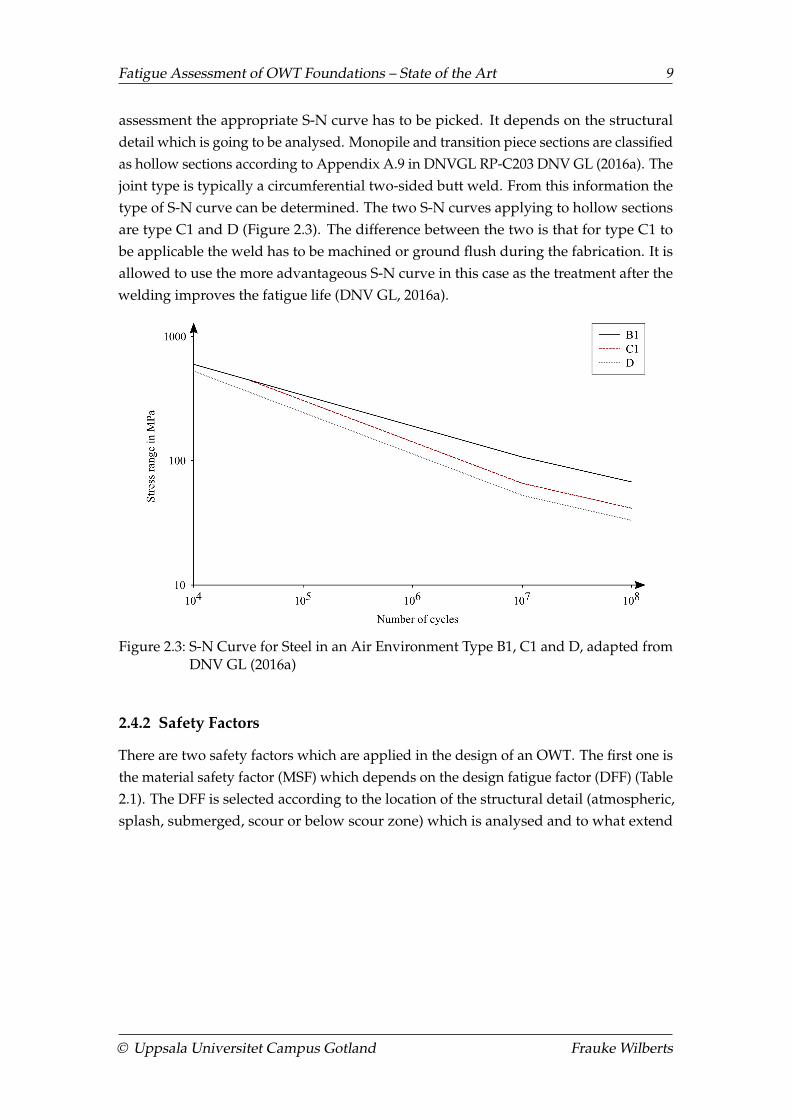
For offshore applications there are three different categories of S-N curves for weldedjoints depending on the environment the steel is placed in: air, water or free corrosion.The S-N curves for the air environment have the highest fatigue life, the water environ-ment (splash zone) has lower fatigue lives and the free corrosion environment (underthe water level) is predicted to have the shortest fatigue life because of the corrosiveenvironment which fosters fatigue damage. In total there are 14 different S-N curvesper environment and curve B1 represents the maximum stress range. For the fatigue
© Uppsala Universitet Campus Gotland Frauke Wilberts
Fatigue Assessment of OWT Foundations – State of the Art 9
assessment the appropriate S-N curve has to be picked. It depends on the structuraldetail which is going to be analysed. Monopile and transition piece sections are classifiedas hollow sections according to Appendix A.9 in DNVGL RP-C203 DNV GL (2016a). Thejoint type is typically a circumferential two-sided butt weld. From this information thetype of S-N curve can be determined. The two S-N curves applying to hollow sectionsare type C1 and D (Figure 2.3). The difference between the two is that for type C1 tobe applicable the weld has to be machined or ground flush during the fabrication. It isallowed to use the more advantageous S-N curve in this case as the treatment after thewelding improves the fatigue life (DNV GL, 2016a).
Figure 2.3: S-N Curve for Steel in an Air Environment Type B1, C1 and D, adapted fromDNV GL (2016a)
2.4.2 Safety Factors
There are two safety factors which are applied in the design of an OWT. The first one isthe material safety factor (MSF) which depends on the design fatigue factor (DFF) (Table2.1). The DFF is selected according to the location of the structural detail (atmospheric,splash, submerged, scour or below scour zone) which is analysed and to what extend
© Uppsala Universitet Campus Gotland Frauke Wilberts

Fatigue Assessment of OWT Foundations – State of the Art 10
regular inspections can and are planned to be carried out (DNV GL, 2016b).
Table 2.1: Design Fatigue Factor and corresponding Material Safety Factor (DNV GL,2016b)
DFF MSF Zone
1 1.0 with inspections (check for cracks every 13 years):atmospheric, splash and submerged zone
2 1.15 with inspections (check for cracks every 7 years):atmospheric, splash and submerged zone
3 1.25 no inspections: atmospheric, splash and submerged zone;always: scour, below scour zone
The second safety factor is the size effect SE. It accounts for differences in the geometryof the test specimen of the S-N curves and the actual geometry. The size effect dependson the wall thickness tw, as a thick section is more likely to fail than a very thin sectionused in the S-N curves. A thickness exponent k which depends on the fatigue strengthis given for every S-N curve within a range of 0 to 0.25 (Equation 2.3). The referencethickness of tre f = 25 mm is applicable for all welded connections (DNV GL, 2016a).
SE =
(tw
tre f
)k
(2.3)
2.4.3 Stress Concentration Factor
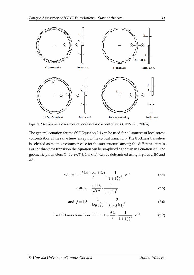
The S-N curves are based on tests of specimen with a uniform stress distribution. Whenusing the S-N curve for a structural detail which does not have a uniform stress dis-tribution but evoke a local stress concentration, changed local stresses are accountedfor by the multiplication of the normal stress with the SCF. Such structural detailswhich can occur as part of the substructure of an OWT are thickness transitions, centereccentricities, concentricity, out of roundness (ovality) and conical transitions from onesection to the other (Figure 2.4).
© Uppsala Universitet Campus Gotland Frauke Wilberts
Fatigue Assessment of OWT Foundations – State of the Art 11
Figure 2.4: Geometric sources of local stress concentrations (DNV GL, 2016a)
The general equation for the SCF Equation 2.4 can be used for all sources of local stressconcentration at the same time (except for the conical transition). The thickness transitionis selected as the most common case for the substructure among the different sources.For the thickness transition the equation can be simplified as shown in Equation 2.7. Thegeometric parameters (δt,δm,δ0, T, t, L and D) can be determined using Figures 2.4b) and2.5.
SCF = 1 +6 (δt + δm + δ0)
t· 1
1 +( T
t
)β· e−α (2.4)
with α =1.82 L√
Dt· 1
1 +( T
t
)β(2.5)
and β = 1.5− 1log(D
t
) + 3(log(D
t
))2 (2.6)
for thickness transition: SCF = 1 +6δt
t· 1
1 +( T
t
)β· e−α (2.7)
© Uppsala Universitet Campus Gotland Frauke Wilberts

Fatigue Assessment of OWT Foundations – State of the Art 12
Figure 2.5: Parameters for the Calculation of the Stress Concentration Factor forThickness Transitions (DNV GL, 2016a)
For the conical transition (Figure 2.6, which also is a common structural detail in OWTsubstructures, there is a different approach of calculation used (Equation 2.8, simplifiedassuming the wall thickness stays constant). The parameters are the diameter of thecylindrical part at the junction Dj, the wall thickness t and the slope angle α.
Figure 2.6: Parameters for the Calculation of the Stress Concentration Factor for ConicalTransitions (DNV GL, 2016a)
SCF = 1 +0.6 t
√Dj · 2t
t2 tanα (2.8)
2.4.4 Rainflow Counting
The first steps of picking the applicable S-N curve and correct it by the safety factorsand a stress concentration factor of the weld detail have been explained. In order to beable to use the S-N curve for the fatigue assessment the two unknowns which are thenumber of cycles N and the corresponding stress range σ have to be determined. This isdone using a method called rainflow counting. The name derives from the basic idea ofcounting rain drops which fall from rooftop to rooftop (Figure 2.7 (b)). Rychlik (1987)adopted the method which was developed by M. Matsuishi and T. Endo in 1968. Hiswork is the basis of the later used MATLAB toolbox WAFO (Chapter 3.2.1) (A. Brodtkorbet al., 2011). The idea of the RFC is to use the strain signal (Figure 2.7 (a)) which shows adynamic load with varying amplitudes over time and convert it into countable stresscycles. This is illustrated by turning the graph of the signal by 90° and then pretendingto let rain flow down from the start of the signal to the end (Figure 2.7 (b)). There arefixed rules as to when a raindrop is stopping or how far it is falling. The horizontalarrows mark the amplitude of the strain and by counting how many times a certain
© Uppsala Universitet Campus Gotland Frauke Wilberts

Fatigue Assessment of OWT Foundations – State of the Art 13
strain amplitude is occurring a histogram of number of times per strain amplitude iscalculated. Thus the result of a RFC algorithm is a bin count, in this case number ofcycles per strain range.
Figure 2.7: Rainflow Counting Method (a) for a Strain Signal and (b) illustrated as aRainflow over Rooftops, adapted from Rychlik (1987)
2.4.5 Miner’s rule
The core idea of the linear damage accumulation lies within the Miner’s rule (Equation2.1): it is assumed that all damage contributions of single stress cycles which occur agiven number of times can be summed up to one damage value.
Figure 2.8: (a) Damage Accumulation Process (adapted from DNV GL (2016a)) and (b)resulting Damage Contributions
In Figure 2.8 (a) the damage accumulation process is demonstrated. It shows on theleft-hand side the fatigue spectrum resulting from the RFC and the applicable S-N curve.The two graphs can be used to determine the values for ni and Ni for every stress bin σi.From the curve of the fatigue spectrum, the number of cycles to failure Ni can be read bydrawing a horizontal line towards the intercept with the S-N curve. Figure 2.8 (b) shows
© Uppsala Universitet Campus Gotland Frauke Wilberts
Fatigue Assessment of OWT Foundations – State of the Art 14
the contributions of each stress bin to the overall damage. With the vertical line at d = 1,the fatigue limit is shown. Comparing the two graphs (Figure 2.8 (a) and (b)), it can beseen that a low number of very high stress cycles causes a higher damage than a highnumber of low stress cycles.
2.4.6 Damage Equivalent Load
The damage equivalent load (DEL) is a measure which enables the comparison ofdifferent fatigue load spectrums. The slope of the S-N curve m and the number of cyclesNeq are getting fixed. From the damage calculated it can then be determined whichconstant amplitude would have generated the same amount of damage based on thefixed parameters, k as the number of stress blocks and Ni as number of cycles to failureat constant stress range (Hendriks and Bulder, 1995).
DEL =
(k
∑i=1
(Ni σ)m
Neq
) 1m
(2.9)
2.5 Summary
From this state of the art overview it can be seen that the fatigue is a design driver forOWT substructures. Although the classical S-N curve approach with a linear damageaccumulation has shortcomings which are based on the one hand on the old data usedfor the curves and on the other hand on the method of summing up damages whichdoes not allow for accounting sequence effects and crack retardation there is not anadequate substitute which can be applied this universally. Therefore, the linear damageaccumulation model will also be used during the following analyses.
In contrast to the majority of fatigue analyses which are based on simulation modelsand determining the design fatigue life, the method used in this thesis is focussing onmeasurement data. Another focus in addition to the fatigue assessment itself is a lookat different operational cases and how they influence the lifetime of an OWT ratherthan collecting data isolated from the load scenario. There is evidence that an idlingOWT experiences higher fatigue loads than being in operation (Vorpahl et al., 2013).The last addition to the current fatigue assessment method is a separate sensitivityanalysis of the geometric properties (wall thickness, diameter and slope angle) of a weldof the monopile and how they influence the correction factors according to the recentguidelines for design (DNVGL RP-C203).
© Uppsala Universitet Campus Gotland Frauke Wilberts
Methodology 15
3 Methodology
3.1 Overview
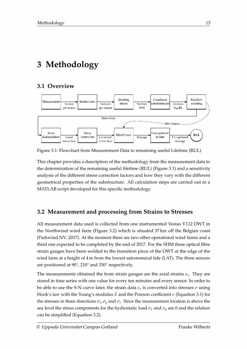
Figure 3.1: Flowchart from Measurement Data to remaining useful Lifetime (RUL)
This chapter provides a description of the methodology from the measurement data tothe determination of the remaining useful lifetime (RUL) (Figure 3.1) and a sensitivityanalysis of the different stress correction factors and how they vary with the differentgeometrical properties of the substructure. All calculation steps are carried out in aMATLAB script developed for this specific methodology.
3.2 Measurement and processing from Strains to Stresses
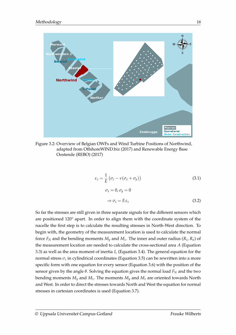
All measurement data used is collected from one instrumented Vestas V112 OWT inthe Northwind wind farm (Figure 3.2) which is situated 37 km off the Belgian coast(Parkwind NV, 2017). At the moment there are two other operational wind farms and athird one expected to be completed by the end of 2017. For the SHM three optical fibrestrain gauges have been welded to the transition piece of the OWT at the edge of thewind farm at a height of 4 m from the lowest astronomical tide (LAT). The three sensorsare positioned at 90°, 210° and 330° respectively.
The measurements obtained the from strain gauges are the axial strains εz. They arestored in time series with one value for every ten minutes and every sensor. In order tobe able to use the S-N curve later, the strain data εz is converted into stresses σ usingHook’s law with the Young’s modulus E and the Poisson coefficient ν (Equation 3.1) forthe stresses in three directions σx,σy and σz. Since the measurement location is above thesea level the stress components for the hydrostatic load σx and σy are 0 and the relationcan be simplified (Equation 3.2).
© Uppsala Universitet Campus Gotland Frauke Wilberts
Methodology 16
Figure 3.2: Overview of Belgian OWFs and Wind Turbine Positions of Northwind,adapted from OffshoreWIND.biz (2017) and Renewable Energy BaseOostende (REBO) (2017)
εz =1E(σz − ν(σx + σy)
)(3.1)
σx = 0, σy = 0
⇒ σz = E εz (3.2)
So far the stresses are still given in three separate signals for the different sensors whichare positioned 120° apart. In order to align them with the coordinate system of thenacelle the first step is to calculate the resulting stresses in North-West direction. Tobegin with, the geometry of the measurement location is used to calculate the normalforce FN and the bending moments My and Mz. The inner and outer radius (Ri, Ro) ofthe measurement location are needed to calculate the cross-sectional area A (Equation3.3) as well as the area moment of inertia Ic (Equation 3.4). The general equation for thenormal stress σz in cylindrical coordinates (Equation 3.5) can be rewritten into a morespecific form with one equation for every sensor (Equation 3.6) with the position of thesensor given by the angle θ. Solving the equation gives the normal load FN and the twobending moments My and Mz. The moments My and Mz are oriented towards Northand West. In order to direct the stresses towards North and West the equation for normalstresses in cartesian coordinates is used (Equation 3.7).
© Uppsala Universitet Campus Gotland Frauke Wilberts
Methodology 17
A = π(R2o − R2
i ) (3.3)
Ic =π
4(R4
o − R4i ) (3.4)
σz =FN
A+
Ri
Ic(My sinθ −Mz cosθ) (3.5)
σz1
σz2
σz3
=
1A
RiIc
sinθ1 −RiIc
cosθ11A
RiIc
sinθ2 −RiIc
cosθ21A
RiIc
sinθ3 −RiIc
cosθ3
FN
My
Mz
(3.6)
σNorth = MyRi
Ic, σWest = Mz
Ri
Ic(3.7)
In the last step the stresses are rotated from the North-West orientation towards a Fore-Aft and Side-Side orientation depending on the yaw angle Ψ by multiplying the stressvalues with the rotation matrix R (Equation 3.8). It puts the values into the nacelle’sframe of reference which always follows the current wind direction (Equation 3.9).
R =
[cos(−Ψ + 180◦) sin(−Ψ + 180◦)−sin(−Ψ + 180◦) cos(−Ψ + 180◦)
](3.8)
σMtl = σNorth · R, σMtn = σWest · R (3.9)
3.2.1 Rainflow counting
In order to obtain the number of cycles per stress level the stresses are counted withthe rainflow counting algorithm (Chapter 2.4.4). A MATLAB toolbox called WAFO,provided by the Centre for Mathematical Sciences at Lund University, is used for therainflow counting (P. Brodtkorb et al., 2000). The research by Rychlik (1987) is the basisfor this MATLAB toolbox. The steps are (1) find the turning points of the stress signals,(2) do the rainflow count, (3) transfer the bins ranges to amplitudes and (4) store theresults of the RFC as histogram data. In contrast to the default method provided byWAFO, stress cycles that are below the lowest stress bin are included in the lowest bin.Otherwise they would be excluded from the count.
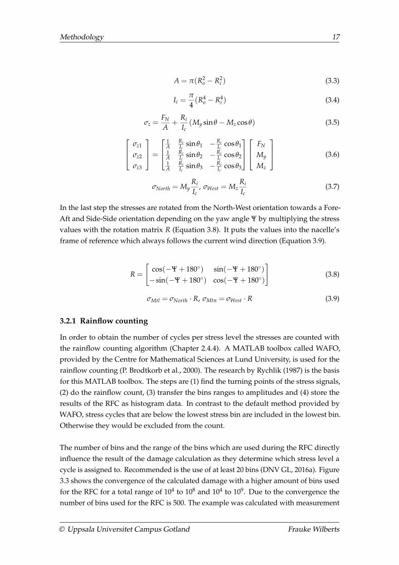
The number of bins and the range of the bins which are used during the RFC directlyinfluence the result of the damage calculation as they determine which stress level acycle is assigned to. Recommended is the use of at least 20 bins (DNV GL, 2016a). Figure3.3 shows the convergence of the calculated damage with a higher amount of bins usedfor the RFC for a total range of 104 to 108 and 104 to 109. Due to the convergence thenumber of bins used for the RFC is 500. The example was calculated with measurement
© Uppsala Universitet Campus Gotland Frauke Wilberts
Methodology 18
data of one day using the S-N curve D in air environment from DNVGL-RP-C203(2016)(DNV GL, 2016a).
Figure 3.3: Convergence of Damage depending on Number of Bins used for RainflowCounting with a Bin Range of 104 to 108 and 104 to 109
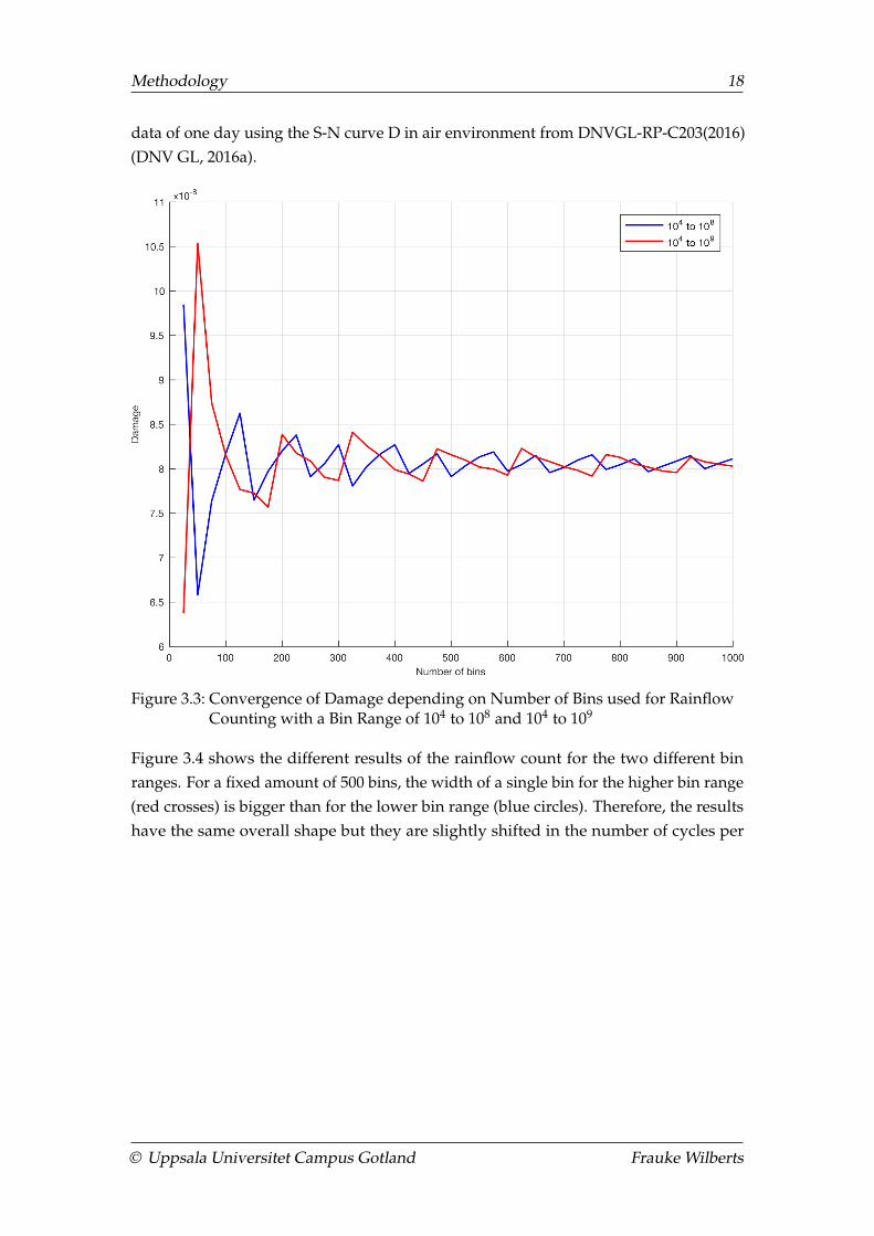
Figure 3.4 shows the different results of the rainflow count for the two different binranges. For a fixed amount of 500 bins, the width of a single bin for the higher bin range(red crosses) is bigger than for the lower bin range (blue circles). Therefore, the resultshave the same overall shape but they are slightly shifted in the number of cycles per
© Uppsala Universitet Campus Gotland Frauke Wilberts
Methodology 19
stress bin.
Figure 3.4: Results for the Rainflow Count for different Ranges of Bins from 104 to either108 or 109
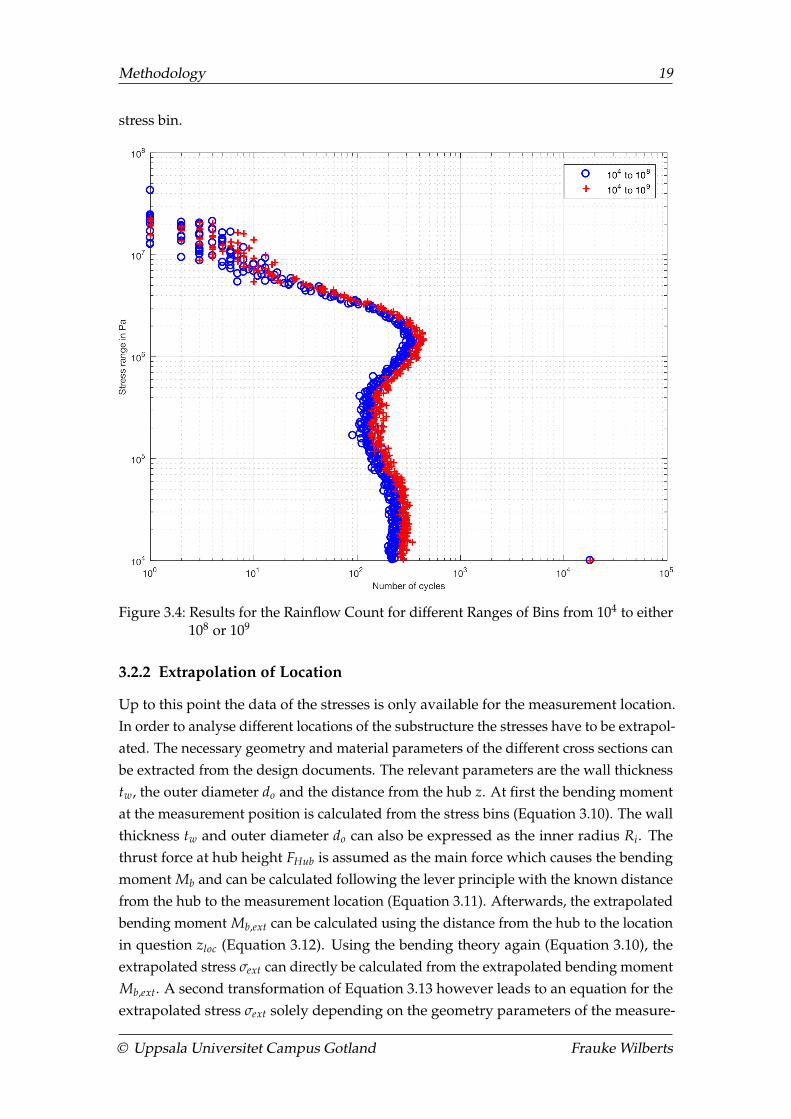
3.2.2 Extrapolation of Location
Up to this point the data of the stresses is only available for the measurement location.In order to analyse different locations of the substructure the stresses have to be extrapol-ated. The necessary geometry and material parameters of the different cross sections canbe extracted from the design documents. The relevant parameters are the wall thicknesstw, the outer diameter do and the distance from the hub z. At first the bending momentat the measurement position is calculated from the stress bins (Equation 3.10). The wallthickness tw and outer diameter do can also be expressed as the inner radius Ri. Thethrust force at hub height FHub is assumed as the main force which causes the bendingmoment Mb and can be calculated following the lever principle with the known distancefrom the hub to the measurement location (Equation 3.11). Afterwards, the extrapolatedbending moment Mb,ext can be calculated using the distance from the hub to the locationin question zloc (Equation 3.12). Using the bending theory again (Equation 3.10), theextrapolated stress σext can directly be calculated from the extrapolated bending momentMb,ext. A second transformation of Equation 3.13 however leads to an equation for theextrapolated stress σext solely depending on the geometry parameters of the measure-
© Uppsala Universitet Campus Gotland Frauke Wilberts

Methodology 20
ment location and the desired location (Equation 3.14). In a final step these parametersare summarised in a static extrapolation factor SEF which can be used to transfer thestress bins of the measurement location to any other location of the substructure viastatic extrapolation (Equation 3.15).
Mb = σIc
do − 2tw= σ
Ic
Ri(3.10)
FHub =Mb
z(3.11)
⇒ Mb,ext = FHub · zloc =Mb
z· zloc (3.12)
σext = Mb,extRi,loc
Ic,loc= Mb ·
zloc
z· Ri,loc
Ic,loc(3.13)
⇒ σext = σ · Ic
Ic,loc· Ri,loc
Ri· zloc
z(3.14)
⇒ SEF =Ic
Ic,loc· Ri,loc
Ri· zloc
z(3.15)
3.2.3 Calculation of Correction Factors
The stress bins resulting from the RFC are directly based on the measured strains andhave so far been adjusted to match the frame of reference of the nacelle and afterwardsbeen extrapolated statically. There are however two other corrections which have to beapplied to them. First of all there are two different safety factors according to DNV GL(2016a) and DNV GL (2016b) (Chapter 2.4.2). These are the MSF and the size effect (SE).Furthermore, there is the SCF which adjusts the stress induced and measured in theclean section to the weld detail by adjusting it to the local expected stress (Chapter 2.4.3).Depending on the structural detail and the geometry the methods for the calculationdiffer among the welds of the substructure. For the case study a fictitious weld betweentwo monopile segments with different wall thicknesses will be analysed. There thesimplified equation (Equation 2.7) can be used. The corrected stress is calculated bymultiplying the stress bins with the MSF, SE and SCF (Equation 3.16).
σcorr = σext ·MSF · SE · SCF (3.16)
3.3 Calculation of Damage
After the RFC there are two counts for the stress bins, one induced by the bendingmoment Mtl and one induced by Mtn. They can now be used to determine how highthe damaging impact on the substructure at the desired location is. For the sake of
© Uppsala Universitet Campus Gotland Frauke Wilberts
Methodology 21
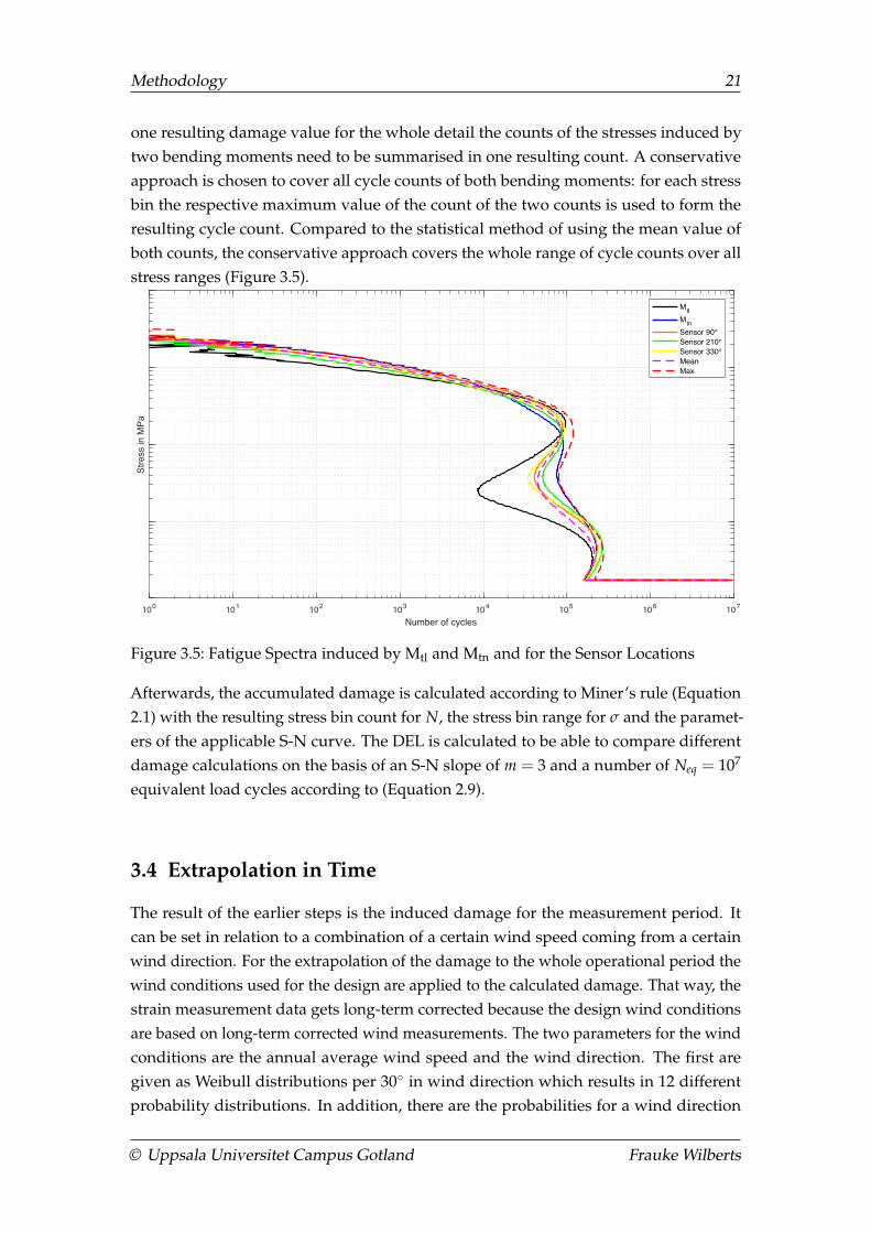
one resulting damage value for the whole detail the counts of the stresses induced bytwo bending moments need to be summarised in one resulting count. A conservativeapproach is chosen to cover all cycle counts of both bending moments: for each stressbin the respective maximum value of the count of the two counts is used to form theresulting cycle count. Compared to the statistical method of using the mean value ofboth counts, the conservative approach covers the whole range of cycle counts over allstress ranges (Figure 3.5).
100 101 102 103 104 105 106 107
Number of cycles
Stre
ss in
MPa
Fatigue spectrum TP_WFBG_LAT04_Mtl_CycleCount & TP_WFBG_LAT04_Mtn_CycleCount
MtlMtnSensor 90°Sensor 210°Sensor 330°MeanMax
Figure 3.5: Fatigue Spectra induced by Mtl and Mtn and for the Sensor Locations
Afterwards, the accumulated damage is calculated according to Miner’s rule (Equation2.1) with the resulting stress bin count for N, the stress bin range for σ and the paramet-ers of the applicable S-N curve. The DEL is calculated to be able to compare differentdamage calculations on the basis of an S-N slope of m = 3 and a number of Neq = 107
equivalent load cycles according to (Equation 2.9).
3.4 Extrapolation in Time
The result of the earlier steps is the induced damage for the measurement period. Itcan be set in relation to a combination of a certain wind speed coming from a certainwind direction. For the extrapolation of the damage to the whole operational period thewind conditions used for the design are applied to the calculated damage. That way, thestrain measurement data gets long-term corrected because the design wind conditionsare based on long-term corrected wind measurements. The two parameters for the windconditions are the annual average wind speed and the wind direction. The first aregiven as Weibull distributions per 30◦ in wind direction which results in 12 differentprobability distributions. In addition, there are the probabilities for a wind direction
© Uppsala Universitet Campus Gotland Frauke Wilberts

Methodology 22
occurring during a year. Multiplying the calculated damage with the probabilities fora given wind speed from a given wind direction gives the expected damage for thosewind conditions. The sum of all individual damages results in the total expected damagefor the measurement period. By multiplying the expected damage with a time factor toreach the total operational time the total expected damage over the lifetime of the OWTcan be calculated.
Dexp = ∑ D90(wd,ws) · Probability(wd,ws) (3.17)
In contrast to the design wind conditions in the strain measurement data not everycombination of wind speed and wind direction has occurred during the measurements.This means that there is no damage value for those empty bins although there is aprobability that this wind condition might occur at some point during the lifetime ofthe OWT. To assign damages to the empty bins an estimation has to be made as to howhigh the damage would be for that wind condition. This is done by taking the maximumvalue among the damages calculated for the full bins. By multiplying them with theprobabilities of the design wind conditions a comparatively high damage for a veryunlikely wind condition gets corrected.Assuming that with a damage of Dexp = 1 the material would fail, the RUL can becalculated (Equation 3.18) using the corresponding time frame texp of the extrapolation.
RUL =texp
Dexp− texp (3.18)
3.5 Case Definitions
As Kallehave et al. (2015) state there’s a difference of damage being induced for an OWTin operation or during stand-still. In order to be able to analyse differences in the damagecalculations, the strain measurements get classified according to 10 different cases whichare determined by the wind speed ws, the revolutions per minute (rpm), the pitch angleϕ and the power output P (Table 3.1). Cases marked "caseless" cannot be categorised ac-cording to the mentioned parameters. They are connected to either an abnormal turbinebehaviour (during curtailment/downrating), or indicate a transition in the behaviour ofthe turbine (e.g. rotor start and stop). All of the parameters can be extracted from theSCADA system of the wind turbine. Cases that are marked with yellow are summarised
© Uppsala Universitet Campus Gotland Frauke Wilberts

Methodology 23
as "idle" and the green cases are considered "operational" in the later analysis (Chapter 4).
Table 3.1: Case Definitions for V112 determined by SCADA Parameters
No. Name ws in m/s rpm ϕ in ° P in MWmin. max. min. max. min. max. min. max.
1 pitch: > 80 - - - 2.5 80 100 - -2 pitch: ± 80 0 22 - 2.5 70 80 - -3 pitch: ± 14 - - - - 14 15 - 0.54 rpm: < 8 - - 2.5 7.9 -4 14 - -5 rpm: ± 8 - - 7.9 8.2 - - - -6 rpm: < 14 - - 8.2 13.6 - - - -7 rpm: ± 14 - - 13.6 14.5 - - - 2.988 max. power - - 13.6 14.5 - - 2.98 -9 cut-out 22 - - - 80 100 - -
10 caseless - - - - - - - -
3.6 Introduction of Sensitivity Analysis of Correction Factors
In addition to the fatigue assessment there is a quick reference tool being developedto allow the influence of different geometrical properties on the SE and the SCF. Theresults can be found in Chapter 4.1. The analysis is based on the equations given inDNVGL-RP-C203 (DNV GL, 2016a).
Table 3.2: Properties used for the Sensitivity Analysis
Property Range
Above weldInner diameter 3900 mm to 4900 mmOuter diameter 4000 mm to 5000 mmWall thickness 35 mm to 70 mmSection height 2700 mm to 5500 mm
Below weldInner diameter 3900 mm to 4900 mmOuter diameter 4000 mm to 5000 mmWall thickness 40 mm to 75 mmMisalignment 1.75 mm to 5 mm
© Uppsala Universitet Campus Gotland Frauke Wilberts

Methodology 24
3.7 Summary
In the methodology it is explained how the fatigue assessment of an OWT starting fromstrain measurements is done. First of all, the strain data has to be transferred into stresseswhich are then put into the frame of reference of the nacelle. In order to use the S-Ncurves for the damage calculation, the stress cycles are counted with a RFC algorithm.Later on, the stresses get extrapolated from the measurement location to the desiredlocation of the substructure and correction factors from design are applied. In the laststep the damage of the stresses is calculated using Miner’s rule and extrapolated in timewith the design wind conditions. Afterwards the RUL can be calculated. Moreover, thegeometrical parameters for a sensitivity analysis of the different correction factors aregiven. The following chapter will demonstrate the results of this methodology appliedto an exemplary weld of an OWT in the Belgian wind farm Northwind. The results willmoreover show how different environmental factors influence the damage induced inthe substructure of the OWT. These are the wind speed, the wind direction, the waveheight, the misalignment between wind direction and wave direction and the turbulenceintensity.
© Uppsala Universitet Campus Gotland Frauke Wilberts

Case Study Results & Discussion 25
4 Case Study Results & Discussion
4.1 Sensitivity Analysis of Stress Correction Factors
In Chapter 2.4.3 the stress concentration factors were introduced. In order to be able toexamine their influence on the stress correction the SCFs for concentricity, center eccent-ricity, out of roundness, thickness transitions (Figure 2.4) and conical transitions (Figure2.6) and the size effect were calculated for different ranges of geometrical properties asdescribed in Chapter 3.6.
Following Equation (2.4) the SCFs of the concentricity, center eccentricity and out ofroundness can be summarised in one graph because they all depend on the deviationδm (Figure 4.1). The resulting SCF for a range of different wall thickness t (in mm) anddifferent misalignments δm increases linearly with the two parameters.
Figure 4.1: Stress Concentration Factors for Concentricity, Center Eccentricity and Outof Roundness
Thickness transitions are a common structural detail of OWT substructures and are usedin the optimisation process to reduce the material and thus the weight of the structure.
© Uppsala Universitet Campus Gotland Frauke Wilberts
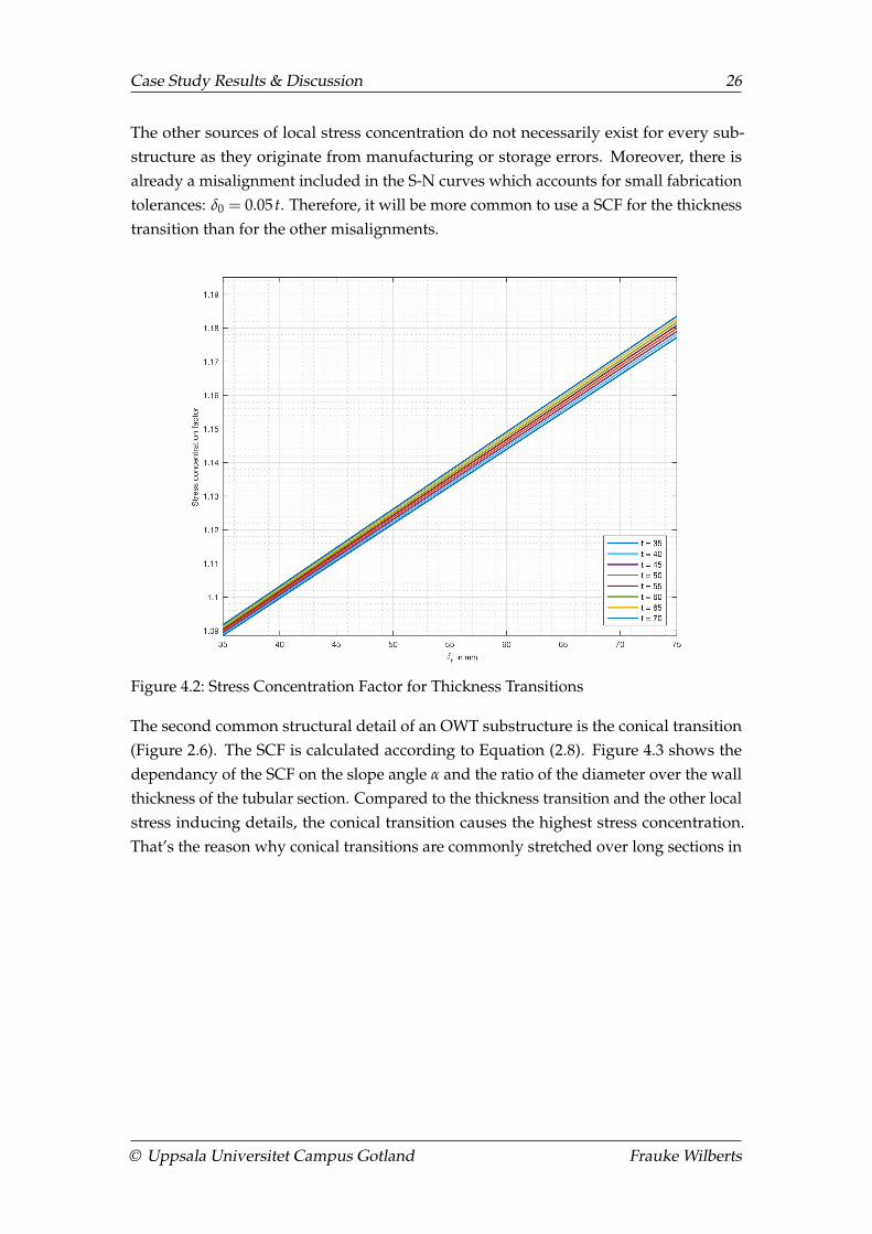
Case Study Results & Discussion 26
The other sources of local stress concentration do not necessarily exist for every sub-structure as they originate from manufacturing or storage errors. Moreover, there isalready a misalignment included in the S-N curves which accounts for small fabricationtolerances: δ0 = 0.05 t. Therefore, it will be more common to use a SCF for the thicknesstransition than for the other misalignments.
Figure 4.2: Stress Concentration Factor for Thickness Transitions
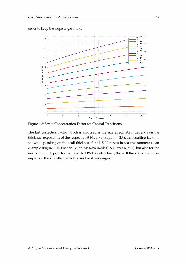
The second common structural detail of an OWT substructure is the conical transition(Figure 2.6). The SCF is calculated according to Equation (2.8). Figure 4.3 shows thedependancy of the SCF on the slope angle α and the ratio of the diameter over the wallthickness of the tubular section. Compared to the thickness transition and the other localstress inducing details, the conical transition causes the highest stress concentration.That’s the reason why conical transitions are commonly stretched over long sections in
© Uppsala Universitet Campus Gotland Frauke Wilberts
Case Study Results & Discussion 27
order to keep the slope angle α low.
Figure 4.3: Stress Concentration Factor for Conical Transitions
The last correction factor which is analysed is the size effect. As it depends on thethickness exponent k of the respective S-N curve (Equation 2.3), the resulting factor isshown depending on the wall thickness for all S-N curves in sea environment as anexample (Figure 4.4). Especially for less favourable S-N curves (e.g. F), but also for themost common type D for welds of the OWT substructures, the wall thickness has a clearimpact on the size effect which raises the stress ranges.
© Uppsala Universitet Campus Gotland Frauke Wilberts

Case Study Results & Discussion 28
Figure 4.4: Size Effect for different S-N Curves in Sea Environment based onRP-C203(2016) (DNV GL, 2016a)
In general the stress correction factors clearly depend on the local geometry and theoverall size of the substructure. For simple tubular sections there is no local stress whichhas to be included in the calculations, the only applicable factor is the size effect. Assoon as there is a thickness transition or a conical transition the local stresses changeconsiderably. The following sections will again focus on the fatigue analysis and usegeometric parameters which are common for monopiles. The examined weld includes athickness transition that induces a local stress concentration which is accounted for bythe appropriate SCF.
4.2 Available Data for the Fatigue Analysis
The following fatigue analysis is based on measurement data over 9 months from theNorthwind wind farm and applied to a fictitious weld between two sections of themonopile, as the original design geometries are confidential. The chosen geometriesare however representative for the actual design. Apart from the measured strains, the
© Uppsala Universitet Campus Gotland Frauke Wilberts
Case Study Results & Discussion 29
following data is available for the analysis (Table 4.1) with 10 minute average values forall measurement data (except for the standard deviation of the wind speed).
Table 4.1: Data used for the Fatigue Assessment
Parameter Unit Origin
Wind speed m/s SCADAStandard deviation of wind speed m/s SCADAWind direction ° SCADAWave height cm OHVS BelwindWave direction high frequency ° Metstation Bol van HeistWave direction low frequency ° Metstation Bol van HeistCases - processed SCADA data
The geometry data used from the measurement location xm and the fictitious weld xw
is summarised in Table 4.2. In order to be able to analyse the effect of a local stressconcentration on the results, a thickness transition from the lower to the higher sectionof the weld at the fictitious location is assumed.
Table 4.2: Properties used for the Fatigue Assessment
Property Size Unitxm xw
Young modulus 210 GPaDFF 3 -S-N curve D for air -Inner diameter 4900 4870 mmOuter diameter 5000 5000 mmWall thickness 50 70 -> 65 mmDistance to hub 78.4 100.4 m
Combining the results of the fatigue analysis with the different environmental factorsthe influence of the respective factors on the damage on the OWT can be investigated.The factors are the wind speed, the wind direction, the wave height, the misalignmentbetween wind direction and wave direction and the turbulence intensity.
4.3 Analysis of Environmental Influences on the Damage
The damage of the 9 months data from Northwind is calculated following the method-ology described in Chapter 3 which is based on the linear damage accumulation (seeChapter 2.4.5). In the following section the results will be shown in resulting graphs,comparing and discussing different influencing factors and their relationship. Due
© Uppsala Universitet Campus Gotland Frauke Wilberts
Case Study Results & Discussion 30
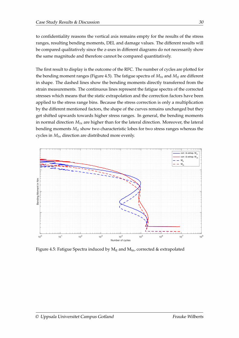
to confidentiality reasons the vertical axis remains empty for the results of the stressranges, resulting bending moments, DEL and damage values. The different results willbe compared qualitatively since the z-axes in different diagrams do not necessarily showthe same magnitude and therefore cannot be compared quantitatively.
The first result to display is the outcome of the RFC. The number of cycles are plotted forthe bending moment ranges (Figure 4.5). The fatigue spectra of Mtn and Mtl are differentin shape. The dashed lines show the bending moments directly transferred from thestrain measurements. The continuous lines represent the fatigue spectra of the correctedstresses which means that the static extrapolation and the correction factors have beenapplied to the stress range bins. Because the stress correction is only a multiplicationby the different mentioned factors, the shape of the curves remains unchanged but theyget shifted upwards towards higher stress ranges. In general, the bending momentsin normal direction Mtn are higher than for the lateral direction. Moreover, the lateralbending moments Mtl show two characteristic lobes for two stress ranges whereas thecycles in Mtn direction are distributed more evenly.
100 101 102 103 104 105 106 107 108
Number of cycles
Bend
ing
Mom
ent i
n N
m
Fatigue spectrum TP_WFBG_LAT04_Mtl_CycleCount & TP_WFBG_LAT04_Mtn_CycleCount
corr. & extrap. M tlcorr. & extrap. M tnMtlMtn
Figure 4.5: Fatigue Spectra induced by Mtl and Mtn, corrected & extrapolated
© Uppsala Universitet Campus Gotland Frauke Wilberts

Case Study Results & Discussion 31
0 3 6 8 11 14 17 19 22 25Wind speed in m/s
50
100
150
200
250
300
350W
ave
heig
ht in
cm
Figure 4.6: Relation of Wind Speed to Wave Height
Figure 4.6 shows the almost linear relation of wave height and wind speed. It impliesthat it is permissible to only look at one parameter for the further analysis as the damagecaused will behave in the same way for both of the environmental influences. This is asimplification, and distributions should be considered, but for now it is assumed thatit can be based solely on wave heights because they are strongly correlated. As thewind speed data is available from SCADA measurements, the choice is made to usethe wind speed as the main parameter for the following analyses of the damaging factors.
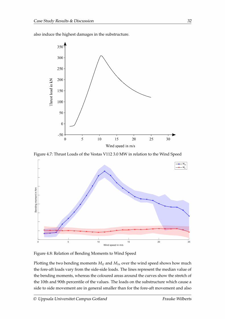
In Figure 4.7 the thrust load of the V112 depending on the wind speed can be seen. Itshows that the maximum thrust load is induced at approximately 11 m/s which should
© Uppsala Universitet Campus Gotland Frauke Wilberts
Case Study Results & Discussion 32
also induce the highest damages in the substructure.
Figure 4.7: Thrust Loads of the Vestas V112 3.0 MW in relation to the Wind Speed
0 5 10 15 20 25Wind speed in m/s
Bend
ing
mom
ent i
n N
m
NWH05
MtnMtl
Figure 4.8: Relation of Bending Moments to Wind Speed
Plotting the two bending moments Mtl and Mtn over the wind speed shows how muchthe fore-aft loads vary from the side-side loads. The lines represent the median value ofthe bending moments, whereas the coloured areas around the curves show the stretch ofthe 10th and 90th percentile of the values. The loads on the substructure which cause aside to side movement are in general smaller than for the fore-aft movement and also
© Uppsala Universitet Campus Gotland Frauke Wilberts

Case Study Results & Discussion 33
stay constant over the wind speed range. As the nacelle is always adjusting its yawangle, the wind always hits the rotor from the front which causes high bending momentsin the fore to aft direction. It can also be seen that the shape of the Mtn curve corres-ponds to the shape of the thrust loads (Figure 4.7) which is related to the relationship ofhigher thrust load causing a higher bending moment. Because the stresses in fore-aftdirection vary much more than the ones in side-side direction the following results aremainly focussing on showing the results for the Mtn direction and the influencing factors.
The following graph shows how the DEL behaves for the two directions of bendingmoments in relation to the wind speed (Figure 4.9). The damage of the OWT gets higherwith an increasing wind speed. This is visible for the stresses induced by Mtl as well asMtn. The difference between the fore-aft and side-side direction is that the variabilityfor Mtn is higher and the DEL is in general a bit higher which is shown by the shadedarea which represents the borders for the 10th and 90th percentile. Especially for thewind speed range of 12 m/s to 13 m/s the damages increase faster than for the rest ofthe wind speed bins.
0 5 10 15 20 25Wind speed in m/s
Dam
age
equi
vale
nt lo
ad in
Nm
NWH05
MtnMtl
Figure 4.9: Influence of Wind Speed on Damage Equivalent Load in Mtl and MtnDirection
The DEL shown in the three dimensional plot (Figure 4.10) represents the 90th percentileof all results binned for wind speeds from 0 m/s to 25 m/s in intervals of 1 m/s and forthe wave heights in 0 cm to 360 cm in intervals of 20 cm. Moreover, there is a thresholdapplied to the bins. If a certain condition determined by the two parameters on thehorizontal axes is not represented at least 5 times in the measurement data the bin isconsidered empty. Thus, very rare conditions are not included in the resulting graph.The method to select the data presented on the vertical axis as 90th percentile and the
© Uppsala Universitet Campus Gotland Frauke Wilberts

Case Study Results & Discussion 34
threshold will be the same for all three dimensional graphs which follow.
Figure 4.10: Influence of Wind Speed and Wave Height on the Damage Equivalent Loadfor all Cases
In Figure 4.10 the influence of the wind speed and the wave height on the DEL in Mtn
direction can be seen. In general, the DEL increases for increasing wind speeds andincreasing wave heights. Only for the wind speed range of 11 m/s to 14 m/s the DEL ishigher than for the neighbouring bins. This can again be connected to the highest thrustloads for these ranges (Figure 4.7).
Concerning the influence of the wave loads on the substructure the following graph(Figure 4.11) considers the directionality of the waves, i.e. if a misalignment betweenthe wave direction and the wind direction induces any recognisable damages in the sub-structure in Mtn direction. The wind/wave misalignment is calculated as the difference
© Uppsala Universitet Campus Gotland Frauke Wilberts
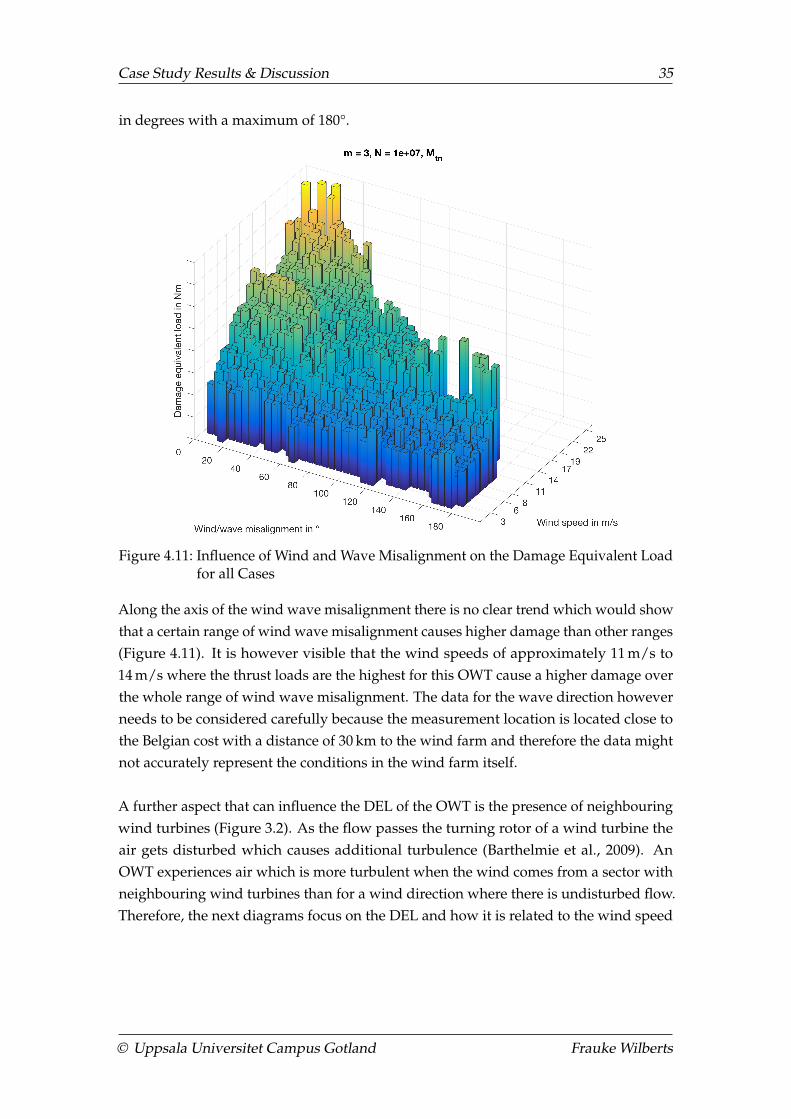
Case Study Results & Discussion 35
in degrees with a maximum of 180°.
Figure 4.11: Influence of Wind and Wave Misalignment on the Damage Equivalent Loadfor all Cases
Along the axis of the wind wave misalignment there is no clear trend which would showthat a certain range of wind wave misalignment causes higher damage than other ranges(Figure 4.11). It is however visible that the wind speeds of approximately 11 m/s to14 m/s where the thrust loads are the highest for this OWT cause a higher damage overthe whole range of wind wave misalignment. The data for the wave direction howeverneeds to be considered carefully because the measurement location is located close tothe Belgian cost with a distance of 30 km to the wind farm and therefore the data mightnot accurately represent the conditions in the wind farm itself.
A further aspect that can influence the DEL of the OWT is the presence of neighbouringwind turbines (Figure 3.2). As the flow passes the turning rotor of a wind turbine theair gets disturbed which causes additional turbulence (Barthelmie et al., 2009). AnOWT experiences air which is more turbulent when the wind comes from a sector withneighbouring wind turbines than for a wind direction where there is undisturbed flow.Therefore, the next diagrams focus on the DEL and how it is related to the wind speed
© Uppsala Universitet Campus Gotland Frauke Wilberts

Case Study Results & Discussion 36
in connection with the wind direction.
Figure 4.12: Influence of Wind Direction and Wind Speed on the Damage EquivalentLoad for Mtn and all Cases
For the wind directions 100° to 220° the DEL for Mtn is considerately lower over almostall wind speeds (Figure 4.12). The only exception is the wind speed range from 14 m/sto 17 m/s where the DEL matches the ones for the other wind directions. The cleardirectionality of the DEL is caused by the adjacent wind turbines. In the range of 100°to 220° there are no neighbouring turbines which would influence the incoming flowbut for the other wind directions it is visible that there are neighbouring turbines whichinduce higher stresses in the substructure caused by the wake (Figure 3.2). In contrast,
© Uppsala Universitet Campus Gotland Frauke Wilberts

Case Study Results & Discussion 37
for the side to side movement of the OWT the neighbouring wind turbines do not havea visible effect (Figure 4.13).
Figure 4.13: Influence of Wind Direction and Wind Speed on the Damage EquivalentLoad for Mtl and all Cases
The following analysis of the turbulence intensity influenced by the wind speed andthe wind direction shows the same directionality and confirms the interpretation ofhigher fatigue loads in Mtn direction (Figure 4.14). As a measurement of turbulence theturbulence intensity TI in % can be used (Equation 4.1). It can be calculated from thewind speed U and the standard deviation of the wind speed std(U) which are includedin the SCADA data of the OWT.
TI =std(U)
U(4.1)
© Uppsala Universitet Campus Gotland Frauke Wilberts
Case Study Results & Discussion 38
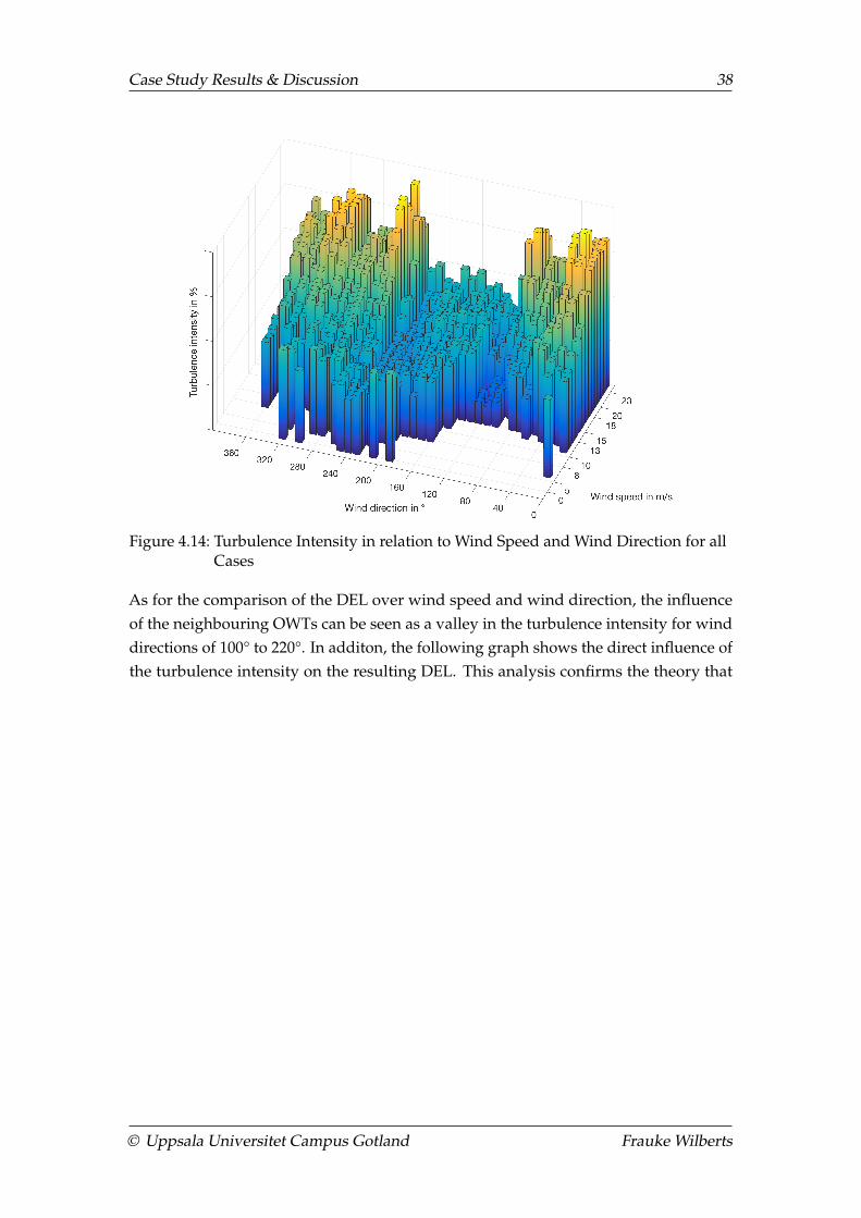
Figure 4.14: Turbulence Intensity in relation to Wind Speed and Wind Direction for allCases
As for the comparison of the DEL over wind speed and wind direction, the influenceof the neighbouring OWTs can be seen as a valley in the turbulence intensity for winddirections of 100° to 220°. In additon, the following graph shows the direct influence ofthe turbulence intensity on the resulting DEL. This analysis confirms the theory that
© Uppsala Universitet Campus Gotland Frauke Wilberts

Case Study Results & Discussion 39
turbulent air increases the fatigue damage of an OWT.
Figure 4.15: Influence of Turbulence Intensity and Wind Speed on the DamageEquivalent Load for all Cases
4.4 Analysis of Damage Results
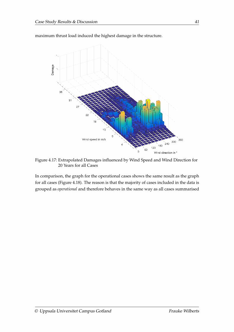
After the analysis of the different environmental influences on the DEL the total extrapol-ated damage for an operation of 20 years is shown. In contrast to the previous analysiswhere the different graphs were based on the results for all cases, in this section thecases all, operational and idle will be distinguished.
In Figure 4.16 the probability distributions for the wind speed and the wind directionfor the site can be seen. The dominant wind sector is south-west for the wind directionbins of 210° to 270°. These wind direction and wind speed probabilities are used for the
© Uppsala Universitet Campus Gotland Frauke Wilberts

Case Study Results & Discussion 40
extrapolation of the damage from the nine months data to 20 years.
Figure 4.16: Design Wind Speed and Wind Direction Probabilities
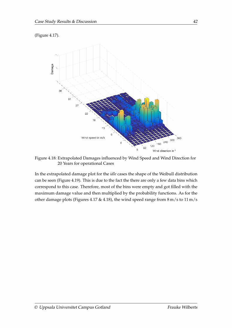
As expected the loads resulting from the wind coming from the south west directionhave the biggest impact on the overall damage of the substructure (Figure 4.17). Thereason is that in those direction the wind speeds are the highest as well as the frequencyin which they occur. The wind speed range from 8 m/s to 11 m/s which is about the
© Uppsala Universitet Campus Gotland Frauke Wilberts
Case Study Results & Discussion 41
maximum thrust load induced the highest damage in the structure.
Figure 4.17: Extrapolated Damages influenced by Wind Speed and Wind Direction for20 Years for all Cases
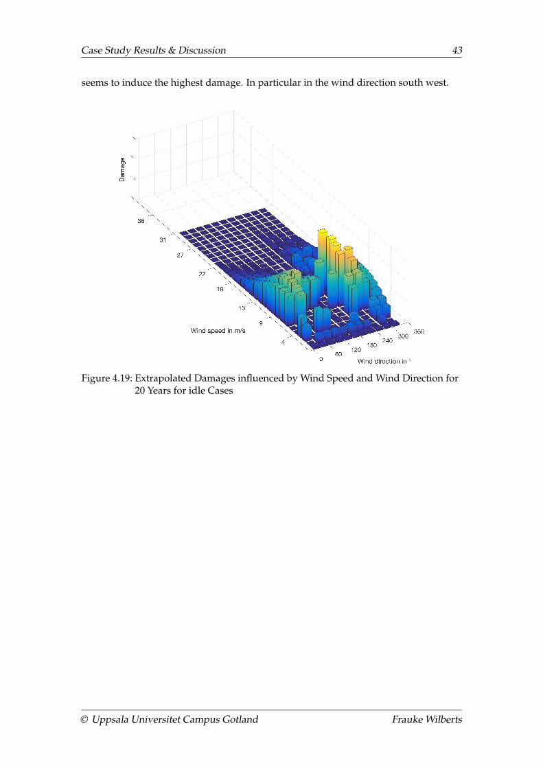
In comparison, the graph for the operational cases shows the same result as the graphfor all cases (Figure 4.18). The reason is that the majority of cases included in the data isgrouped as operational and therefore behaves in the same way as all cases summarised
© Uppsala Universitet Campus Gotland Frauke Wilberts
Case Study Results & Discussion 42
(Figure 4.17).
Figure 4.18: Extrapolated Damages influenced by Wind Speed and Wind Direction for20 Years for operational Cases
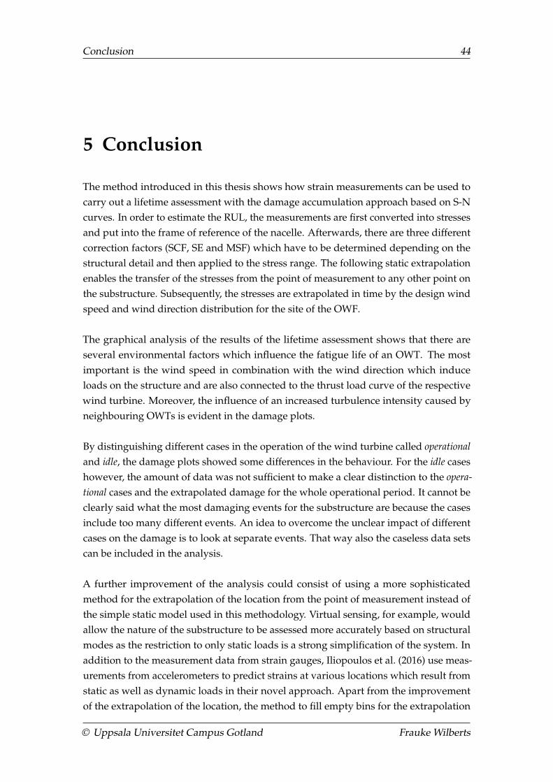
In the extrapolated damage plot for the idle cases the shape of the Weibull distributioncan be seen (Figure 4.19). This is due to the fact the there are only a few data bins whichcorrespond to this case. Therefore, most of the bins were empty and got filled with themaximum damage value and then multiplied by the probability functions. As for theother damage plots (Figures 4.17 & 4.18), the wind speed range from 8 m/s to 11 m/s
© Uppsala Universitet Campus Gotland Frauke Wilberts
Case Study Results & Discussion 43
seems to induce the highest damage. In particular in the wind direction south west.
Figure 4.19: Extrapolated Damages influenced by Wind Speed and Wind Direction for20 Years for idle Cases
© Uppsala Universitet Campus Gotland Frauke Wilberts
Conclusion 44
5 Conclusion
The method introduced in this thesis shows how strain measurements can be used tocarry out a lifetime assessment with the damage accumulation approach based on S-Ncurves. In order to estimate the RUL, the measurements are first converted into stressesand put into the frame of reference of the nacelle. Afterwards, there are three differentcorrection factors (SCF, SE and MSF) which have to be determined depending on thestructural detail and then applied to the stress range. The following static extrapolationenables the transfer of the stresses from the point of measurement to any other point onthe substructure. Subsequently, the stresses are extrapolated in time by the design windspeed and wind direction distribution for the site of the OWF.
The graphical analysis of the results of the lifetime assessment shows that there areseveral environmental factors which influence the fatigue life of an OWT. The mostimportant is the wind speed in combination with the wind direction which induceloads on the structure and are also connected to the thrust load curve of the respectivewind turbine. Moreover, the influence of an increased turbulence intensity caused byneighbouring OWTs is evident in the damage plots.
By distinguishing different cases in the operation of the wind turbine called operationaland idle, the damage plots showed some differences in the behaviour. For the idle caseshowever, the amount of data was not sufficient to make a clear distinction to the opera-tional cases and the extrapolated damage for the whole operational period. It cannot beclearly said what the most damaging events for the substructure are because the casesinclude too many different events. An idea to overcome the unclear impact of differentcases on the damage is to look at separate events. That way also the caseless data setscan be included in the analysis.
A further improvement of the analysis could consist of using a more sophisticatedmethod for the extrapolation of the location from the point of measurement instead ofthe simple static model used in this methodology. Virtual sensing, for example, wouldallow the nature of the substructure to be assessed more accurately based on structuralmodes as the restriction to only static loads is a strong simplification of the system. Inaddition to the measurement data from strain gauges, Iliopoulos et al. (2016) use meas-urements from accelerometers to predict strains at various locations which result fromstatic as well as dynamic loads in their novel approach. Apart from the improvementof the extrapolation of the location, the method to fill empty bins for the extrapolation
© Uppsala Universitet Campus Gotland Frauke Wilberts
Conclusion 45
in time could be changed for an estimation based on the nearest neighbour insteadof simply assuming the maximum damage value. Another simplification in the usedmethod is to assume the substructure only experiences loads while being installed andin operation. In reality, the installation with piling the substructure into the seabedalready induces damage which cannot be included in the fatigue estimation when themeasurements only take place after the installation. It would therefore be useful to havesensors already in place during transport and installation of the OWT.
In order to improve the approach of the linear damage accumulation which has someshortcomings as mentioned in Chapter 2, future work on the topic of assessing the RULcould be based on a crack propagation model which would allow for sequence effectsto be included. It could be an idea to calculate how fast a crack is growing comingfrom a certain weld and compare different initial crack sizes. One outcome could be todetermine at which crack size the structure is not safe anymore and would eventuallyfail by using the extrapolation in time.
© Uppsala Universitet Campus Gotland Frauke Wilberts
Literature 46
Literature
Adedipe, O., F. Brennan and A. Kolios. 2016. ‘Review of corrosion fatigue in offshorestructures: Present status and challenges in the offshore wind sector’. In: Renewableand Sustainable Energy Reviews vol. 61, pp. 141–154.
Barthelmie, R. J., K. Hansen, S. T. Frandsen, O. Rathmann, J. G. Schepers, W. Schlez,J. Phillips, K. Rados, A. Zervos, E. S. Politis and P. K. Chaviaropoulos. 2009.‘Modelling and Measuring Flow and Wind Turbine Wakes in Large Wind FarmsOffshore’. In: Wind Energy vol. 12, pp. 431–444.
Bhattacharya, S. 2014. ‘Challenges in Design of Foundations for Offshore WindTurbines’. In: Engineering & Technology Reference, pp. 1–9.
Brennan, F. and I. Tavares. 2014. ‘Fatigue design of offshore steel mono-pile windsubstructures’. In: Proceedings of the Institution of Civil Engineers Energyvol. 167.no. EN4, pp. 196–202.
Brodtkorb, A., P. Johannesson, G. Lindgren and I. Rychlik. 2011. WAFO – a MatlabToolbox for Analysis of Random Waves and Loads. Tech. rep. Lund: Lund University.
Brodtkorb, P., P. Johannesson, G. Lindgren, I. Rychlik, J. Rydén and E. Sjö. 2000. ‘WAFO -a Matlab Toolbox for the Analysis of Random Waves and Loads’. In: Proc. 10’th Int.Offshore and Polar Eng. Conf., ISOPE, Seattle, USA. Vol. 3, pp. 343–350.
Det Norske Veritas Germanischer Lloyd (DNV GL). 2016a. DNVGL-RP-C203: Fatiguedesign of offshore steel structures. DNVGL-RP-C203:2016-04.
– 2016b. DNVGL-ST-0126: Support structures for wind turbines. DNVGL-ST-0126:2016-04.
Fatemi, A. and L. Yang. 1998. ‘Cumulative fatigue damage and life prediction theories: asurvey of the state of the art for homogeneous materials’. In: International Journal ofFatigue vol. 20.no. 1, pp. 9–34.
Gengenbach, J., M. Brommundt, K. Mikkelsen, J. S. Gretlund and F. Rüdinger. 2015.‘Design challenges of XL monopiles’. In: EWEA Offshore. Barcelona.
Hendriks, H. B. and B. H. Bulder. 1995. Fatigue Equivalent Load Cycle Method. Tech. rep.ECN-C-95-074. Energy Research Centre of the Netherlands (ECN).
Ho, A. and A. Mbistrova. 2017. The European offshore wind industry, Key trends andstatistics 2016. Tech. rep. Brussels: WindEurope.
© Uppsala Universitet Campus Gotland Frauke Wilberts

Literature 47
International Electrotechnical Commission (IEC). 2015. Wind turbines - Part 13:Measurement of mechanical loads. IEC 61400-13:2015.
Iliopoulos, A. N., W. Weijtjens, D. Van Hemelrijck and C. Devriendt. 2016. ‘Remaininguseful life assessment of offshore wind turbines : Validation of virtual sensing on longterm measurements’. In: 8th European Workshop On Structural Health Monitoring(EWSHM 2016).
Kallehave, D., B. W. Byrne, C. LeBlanc Thilsted and K. K. Mikkelsen. 2015.‘Optimization of monopiles for offshore wind turbines’. In: Philosophical Transactions ofthe Royal Society A vol. 373.
OffshoreWIND.biz. 2017. ’EC Approves Support Scheme for Rentel and Norther OWFs’.http://www.offshorewind.biz/2016/12/09/ec-approves-support-scheme-for-rentel-and-norther-owfs/, accessed 4th September 2017.
Parkwind NV. 2017. ’Overview Projects Parkwind’.http://www.parkwind.eu/en/projects/about?scroll=Northwind, accessed4th September 2017.
Renewable Energy Base Oostende (REBO). 2017. ’Offshore wind farms’.http://www.reboostende.be/offshore-wind-farms, accessed 4th September 2017.
Rychlik, I. 1987. ‘A new definition of the rainflow cycle counting method’. In:International Journal of Fatigue vol. 9.no. 2, pp. 119–121.
Schijve, J. 2003. ‘Fatigue of structures and materials in the 20th century and the state ofthe art’. In: International Journal of Fatigue vol. 25, pp. 679–702.
Söker, H. 1996. ‘Ermittlung von Ermüdungslasten an großen Windenergieanlagen’. In:DEWI Magazin no. 8, pp. 45–48.
Vorpahl, F., H. Schwarze, T. Fischer, M. Seidel and J. Jonkman. 2013. ‘Offshore windturbine environment, loads, simulation, and design’. In: Wiley InterdisciplinaryReviews: Energy and Environment vol. 2, pp. 548–570.
Weijtjens, W., N. Noppe, T. Verbelen, A. Iliopoulos and C. Devriendt. 2016. ‘Offshorewind turbine foundation monitoring, extrapolating fatigue measurements from fleetleaders to the entire wind farm’. In: Journal of Physics: Conference Series. Vol. 753.
Wymore, M. L., J. E. Van Dam, H. Ceylan and D. Qiao. 2015. ‘A survey of healthmonitoring systems for wind turbines’. In: Renewable and Sustainable Energy Reviewsvol. 52, pp. 976–990.
Ziegler, L., S. Schafhirt, M. Scheu and M. Muskulus. 2016. ‘Effect of Load Sequence andWeather Seasonality on Fatigue Crack Growth for Monopile-based Offshore WindTurbines’. In: Energy Procedia vol. 94.no. January, pp. 115–123.
© Uppsala Universitet Campus Gotland Frauke Wilberts

Literature 48
Ziegler, L., U. Smolka, N. Cosack and M. Muskulus. 2017. ‘Structural monitoring forlifetime extension of offshore wind monopiles: Can strain measurements at one leveltell us everything?’ manuscript submitted for publication.
© Uppsala Universitet Campus Gotland Frauke Wilberts