MEASUREMENT OF COSMIC MICROWAVE BACKGROUND POLARIZATION POWER

SPECTRA FROM TWO YEARS OF BICEP DATA

This article has been downloaded from IOPscience. Please scroll down to see the full text article.

2010 ApJ 711 1123

(http://iopscience.iop.org/0004-637X/711/2/1123)

Download details:

IP Address: 131.215.193.213

The article was downloaded on 12/03/2010 at 21:22

Please note that terms and conditions apply.

The Table of Contents and more related content is available

Home Search Collections Journals About Contact us My IOPscience

The Astrophysical Journal, 711:1123–1140, 2010 March 10 doi:10.1088/0004-637X/711/2/1123C© 2010. The American Astronomical Society. All rights reserved. Printed in the U.S.A.

MEASUREMENT OF COSMIC MICROWAVE BACKGROUND POLARIZATION POWER SPECTRA FROM TWOYEARS OF BICEP DATA

H. C. Chiang1,2

, P. A. R. Ade3, D. Barkats

1,4, J. O. Battle

5, E. M. Bierman

6, J. J. Bock

1,5, C. D. Dowell

5, L. Duband

7,

E. F. Hivon8, W. L. Holzapfel

9, V. V. Hristov

1, W. C. Jones

1,2, B. G. Keating

6, J. M. Kovac

1, C. L. Kuo

10,11,

A. E. Lange1,5,15

, E. M. Leitch12

, P. V. Mason1, T. Matsumura

1, H. T. Nguyen

5, N. Ponthieu

13, C. Pryke

12, S. Richter

1,

G. Rocha1,5

, C. Sheehy12

, Y. D. Takahashi9, J. E. Tolan

10,11, and K. W. Yoon

141 Department of Physics, California Institute of Technology, Pasadena, CA 91125, USA

2 Department of Physics, Princeton University, Princeton, NJ 08544, USA3 Department of Physics and Astronomy, University of Wales, Cardiff, CF24 3YB, Wales, UK

4 National Radio Astronomy Observatory, Santiago, Chile5 Jet Propulsion Laboratory, Pasadena, CA 91109, USA

6 Department of Physics, University of California at San Diego, La Jolla, CA 92093, USA7 SBT, Commissariat a l’Energie Atomique, Grenoble, France

8 Institut d’Astrophysique de Paris, Paris, France9 Department of Physics, University of California at Berkeley, Berkeley, CA 94720, USA

10 Stanford University, Palo Alto, CA 94305, USA11 Kavli Institute for Particle Astrophysics and Cosmology (KIPAC), Sand Hill Road 2575, Menlo Park, CA 94025, USA

12 University of Chicago, Chicago, IL 60637, USA13 Institut d’Astrophysique Spatiale, Universite Paris-Sud, Orsay, France

14 National Institute of Standards and Technology, Boulder, CO 80305, USAReceived 2009 June 15; accepted 2010 January 29; published 2010 February 22

ABSTRACT

Background Imaging of Cosmic Extragalactic Polarization (Bicep) is a bolometric polarimeter designed to measurethe inflationary B-mode polarization of the cosmic microwave background (CMB) at degree angular scales. Duringthree seasons of observing at the South Pole (2006 through 2008), Bicep mapped ∼2% of the sky chosen to beuniquely clean of polarized foreground emission. Here, we present initial results derived from a subset of thedata acquired during the first two years. We present maps of temperature, Stokes Q and U, E and B modes, andassociated angular power spectra. We demonstrate that the polarization data are self-consistent by performing aseries of jackknife tests. We study potential systematic errors in detail and show that they are sub-dominant tothe statistical errors. We measure the E-mode angular power spectrum with high precision at 21 � � � 335,detecting for the first time the peak expected at � ∼ 140. The measured E-mode spectrum is consistent withexpectations from a ΛCDM model, and the B-mode spectrum is consistent with zero. The tensor-to-scalar ratioderived from the B-mode spectrum is r = 0.02+0.31

−0.26, or r < 0.72 at 95% confidence, the first meaningfulconstraint on the inflationary gravitational wave background to come directly from CMB B-mode polarization.

Key words: cosmic background radiation – cosmology: observations – gravitational waves – inflation –polarization

Online-only material: color figure

1. INTRODUCTION

One of the cornerstones in our current understanding ofcosmology is the theory of inflation. Inflation addresses severalmajor shortcomings of the standard big bang model, resolvingthe flatness and horizon problems and explaining the originof structure; however, the theory has yet to be unambiguouslyconfirmed by observational evidence.

Numerous experiments have demonstrated that the cosmicmicrowave background (CMB) is an extremely effective toolfor studying the early universe. Precision measurements of thetemperature anisotropies now span a wide range of angularscales (Jones et al. 2006; Reichardt et al. 2009; Nolta et al. 2009;Friedman et al. 2009; Sievers et al. 2009; Brown et al. 2009)and have yielded tight constraints on a model of the universein which the energy content is dominated by a cosmologicalconstant and cold dark matter (ΛCDM).

The polarization anisotropies of the CMB provide even moreinsight into the history of the universe, potentially encoding in-

15 Sadly, Andrew Lange passed away shortly before the publication of thisarticle.

formation from long before the moment of matter–radiationdecoupling. The primary source of CMB polarization isThomson scattering of the local quadrupole of the photon–baryon fluid sourced by density fluctuations. The resulting par-tial polarization has no handedness and is called the gradientor “E-mode” by analogy to curl-free electric fields. The ΛCDMparameters that predict the temperature spectrum also predictthe shape of the E-mode spectrum with almost no additionalinformation (reionization enhances power at the largest angularscales). E-mode polarization was first detected by Dasi (Kovacet al. 2002) and has since been measured by many other exper-iments (Leitch et al. 2005; Montroy et al. 2006; Sievers et al.2007; Wu et al. 2007; Bischoff et al. 2008). The acoustic peaksin the polarization spectra have been measured to high preci-sion in both the TE spectrum (Piacentini et al. 2006; Nolta et al.2009) and, more recently, directly in the EE spectrum (Prykeet al. 2009; Brown et al. 2009), providing further support forour basic understanding of CMB physics.

Inflation predicts the existence of a stochastic gravitationalwave background, created during the initial accelerated expan-sion of the universe, which imparts a unique imprint on the CMB

1123

1124 CHIANG ET AL. Vol. 711

at the surface of last scattering (Polnarev 1985). In addition toproducing E-mode polarization, gravitational waves also inducea curl or “B-mode” in the polarization anisotropies (Seljak &Zaldarriaga 1997; Kamionkowski et al. 1997). The inflation-ary B-mode signal is expected to peak at degree angular scales(multipole moment � ∼ 100) with an amplitude determined bythe energy scale of inflation. Because density fluctuations atthe surface of last scattering create only E-mode polarization, adetection of the B-mode signal would be strong evidence thatinflation occurred (see, e.g., Dodelson et al. 2009).

The inflationary B-mode amplitude is parameterized by thetensor-to-scalar ratio r, and the most restrictive published up-per limit, r < 0.22 (95% confidence), comes from measure-ments of large-scale temperature anisotropies in combinationwith baryon acoustic oscillation and Type Ia supernova data(Komatsu et al. 2009). However, the constraints from tempera-ture anisotropies are ultimately limited by cosmic variance, andlowering the r limit further requires direct polarization mea-surements. Currently, limits from polarization are still far worsethan those from temperature—for example, assuming ΛCDMparameters that are fixed at Wilkinson Microwave AnisotropyProbe (WMAP) best-fit values, the WMAP B-mode spectrumconstrains r < 6 at 95% confidence. The results reported inthis paper provide upper limits on the B-mode signal that are anorder of magnitude more stringent than those set by WMAP.

Background Imaging of Cosmic Extragalactic Polarization(Bicep) is a microwave polarimeter that has been designedspecifically to probe the B-mode of CMB polarization atdegree angular scales. The instrument observed from the SouthPole between 2006 January and 2008 December. A detaileddescription of the Bicep instrument characterization proceduresis given in a companion paper, Takahashi et al. (2010). In thispaper, we report initial CMB polarization results from the 2006and 2007 observing seasons.

2. THE BICEP INSTRUMENT

A complete description of the Bicep instrument is availablein Yoon et al. (2006), and only a brief summary is given here.The Bicep receiver consists of a two-lens refracting telescopecoupled to a focal plane of 49 orthogonal pairs of polarization-sensitive bolometers (PSBs; Jones et al. 2003). The PSB pairs aredivided between 25 that observe at 100 GHz and 24 at 150 GHz(two of the 150 GHz PSB pairs were reconfigured for 220 GHzoperation in late 2006 and were subsequently not used for CMBanalysis). The angular resolution at 100 and 150 GHz is 0.◦93and 0.◦60, respectively, and the instantaneous field of view is18◦. The entire focal plane and optics assembly is housed in anupward-looking cryostat with toroidal liquid nitrogen and liquidhelium tanks. The clean optical path and azimuthal symmetryminimize instrumental polarization systematics.

The receiver is supported in an azimuth–elevation mount witha third degree of rotational freedom about the boresight. Themount is located on the top floor of the Dark Sector Laboratory(89.◦99 S, 44.◦65 W) at the Amundsen–Scott South Pole station,a site with excellent atmospheric transparency and stability atmillimeter wavelengths as well as outstanding infrastructure.The telescope penetrates through the roof and is sealed to thebuilding with a flexible environmental enclosure, leaving mostof the instrument accessible in a warm lab setting.

The 24 hr visibility of the target field from the SouthPole enables uninterrupted observation and deep integration.Bicep’s primary CMB field lies within the “Southern Hole,”

Figure 1. Bicep’s CMB and Galactic fields are outlined on the 150 GHz FDSModel 8 prediction of dust emission (Finkbeiner et al. 1999), plotted here inequatorial coordinates.

a region of low dust emission outlined in Figure 1, in a rightascension and declination range of approximately |α| < 60◦and −70◦ < δ < −45◦. The telescope observation cycle is48 sidereal hours in length and is divided into four 9 hr CMBobservations, 6 hr of Galactic observations, and 6 hr of cryogenservicing. The CMB field is covered twice over the same azimuthrange during each 48 hr cycle, but the elevation halves aremapped in opposite order between the two observations. Theboresight angle in each cycle is held fixed at one of four angles{−45◦, 0◦, 180◦, 135◦} that provide good thermal-microphonicstability and redundant polarization angle coverage.

Bicep maps the sky with azimuth–elevation raster scans.During each complete CMB observation (18 hr), the telescopeboresight steps in elevation between 55◦ and 59.◦75 in 0.◦25increments. At each step in elevation, the telescope performs aset of 50 back-and-forth azimuth scans over a total period of∼50 minutes. The azimuth scan width is 64.◦4, and the speed isheld constant at 2.◦8 s−1 over ∼70% of the scan duration, whichmodulates the sky signal and places it in a frequency band ofapproximately 0.1–1 Hz. The scans have a fixed azimuth centerthat is updated at each elevation step to approximately track thefield center. This scan strategy was chosen instead of continuoustracking in order to allow removal of any azimuth-fixed or scan-synchronous contamination.

Relative detector gains are measured regularly during observ-ing cycles with “elevation nods” performed at the beginning andend of each fixed-elevation scan set. During an elevation nod,the mount performs a rounded triangle wave motion in eleva-tion with a 1.◦2 peak-to-peak amplitude, and the detector voltagesvary in response to the changing line-of-sight air mass. The nodis performed over a 45 s period to reduce thermal disturbanceson the focal plane, and thermal drifts are further suppressed byusing mirror-image elevation nods at the beginning and end ofeach scan set (up-down-up and down-up-down).

No. 2, 2010 CMB POLARIZATION SPECTRA FROM BICEP TWO-YEAR DATA 1125

3. INSTRUMENT CHARACTERIZATION

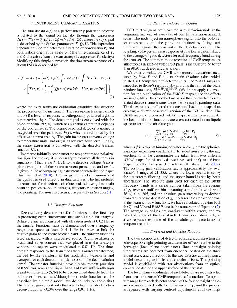
The timestream d(t) of a perfect linearly polarized detectoris related to the signal on the sky through the expressiond(t) = T (rb)+Q(rb) cos 2ψ+U (rb) sin 2ψ , where the sky signalis described by the Stokes parameters T ,Q,U . This expressiondepends only on the detector’s direction of observation rb andpolarization orientation angle ψ . (The time-dependence of rb

and ψ that arises from the scan strategy is suppressed for clarity.)Modifying this simple expression, the timestream response of aBicep PSB is described by

d(t) = K(t) ∗{n(t) + g(t)

∫dνAeF (ν)

∫dr P (r − rb, ν)

×[T (r, ν) +

1 − ε

1 + ε(Q(r, ν) cos 2ψ + U (r, ν) sin 2ψ)

] },

(1)

where the extra terms are calibration quantities that describethe properties of the instrument. The cross-polar leakage, whichis a PSB’s level of response to orthogonally polarized light, isparameterized by ε. The detector signal is convolved with theco-polar beam P (r, ν), which has a spatial extent that dependson the coordinate r. The beam-convolved detector response isintegrated over the pass band F (ν), which is multiplied by theeffective antenna area Ae. The gain factor g(t) converts voltageto temperature units, and n(t) is an additive noise term. Finally,the entire expression is convolved with the detector transferfunction K(t).

In order to faithfully reconstruct the temperature and polariza-tion signal on the sky, it is necessary to measure all the terms inEquation (1) that relate T ,Q,U to the detector voltage. A com-plete description of these measurement procedures and resultsis given in the accompanying instrument characterization paper(Takahashi et al. 2010). Here, we give only a brief summary ofthe quantities used directly in data analysis. The list includesdetector transfer functions, absolute and relative gains, mainbeam shapes, cross-polar leakages, detector orientation angles,and pointing. The noise is discussed separately in Section 6.1.

3.1. Transfer Functions

Deconvolving detector transfer functions is the first stepin producing clean timestreams that are suitable for analysis.Relative gains are measured with elevation nods at 0.02 Hz, sothe transfer functions must be characterized over a frequencyrange that spans at least 0.01–1 Hz in order to link therelative gains to the entire science band. The transfer functionswere measured with a microwave source (Gunn oscillator orbroadband noise source) that was placed near the telescopewindow and square-wave modulated at 0.01 Hz. The time-domain responses to the transitions were Fourier transformed,divided by the transform of the modulation waveform, andaveraged for each detector in order to obtain the deconvolutionkernel. The transfer functions have a measurement precisionof 0.5% rms across the signal band and have sufficiently highsignal-to-noise ratio (S/N) to be deconvolved directly from thebolometer timestreams. (Although the transfer functions can bedescribed by a simple model, we do not rely on those fits.)The relative gain uncertainty that results from transfer functiondeconvolution is <0.3% over the range 0.01–1 Hz.

3.2. Relative and Absolute Gains

PSB relative gains are measured with elevation nods at thebeginning and end of every set of constant-elevation azimuthscans. The nods inject an atmospheric signal into the bolome-ter timestreams, and the gains are obtained by fitting eachtimestream against the cosecant of the detector elevation. Theresulting volts-per-air mass responsivity factors are normalizedto the average of good detectors for each frequency band duringthe scan set. The common-mode rejection of CMB temperatureanisotropies in gain-adjusted PSB pairs is measured to be betterthan 98.9% at degree angular scales.

We cross-correlate the CMB temperature fluctuations mea-sured by WMAP and Bicep to obtain absolute gains, whichrelate CMB temperature to detector units. The WMAP maps aresmoothed to Bicep’s resolution by applying the ratio of the beamwindow functions, BBICEP

� /BWMAP� . (We do not apply a correc-

tion for the pixelization of the WMAP maps since the effectsare negligible.) The smoothed maps are then converted to sim-ulated detector timestreams using the boresight pointing data.The timestreams are filtered and converted back into maps, thuscreating a “Bicep-observed” version of the WMAP data. TheBicep map and processed WMAP maps, which have compati-ble beam and filter functions, are cross-correlated in multipolespace to obtain the absolute gain

gb =∑

� P b�

⟨aWMAP−1

�m a∗ BICEP�m

⟩∑

� P b�

⟨aWMAP−1

�m a∗ WMAP−2�m

⟩ , (2)

where P b� is a top hat binning operator, and a�m are the spherical

harmonic expansion coefficients. To avoid noise bias, the a�m

coefficients in the denominator are taken from two differentWMAP maps; for this analysis, we have used the Q- and V-bandmaps from the five-year data release (Hinshaw et al. 2009).The resulting gain calibration, gb, is approximately flat overBicep’s � range of 21–335, where the lower bound is set bythe timestream filtering, and the upper bound is set by beamuncertainty. The absolute gain used for each of the Bicep

frequency bands is a single number taken from the averageof gb over six uniform bins spanning a multipole window of56 � � � 265, and the absolute gain uncertainty is derivedfrom the standard deviation of gb. To assess the impact of errorsin the beam window functions, we have calculated gb using boththe Q- and V-band WMAP data in the numerator of Equation (2).The average gb values are consistent within errors, and wetake the larger of the two standard deviation values, 2%, asa conservative estimate of the absolute gain uncertainty intemperature units.

3.3. Boresight and Detector Pointing

The two components of detector pointing reconstruction aretelescope boresight pointing and detector offsets relative to theboresight (focal plane coordinates). Raw boresight pointingtimestreams are obtained from encoders located on the threemount axes, and corrections to the raw data are applied from amodel describing axis tilts and encoder offsets. The pointingmodel is established with star observations from an opticalcamera located on the upper surface of the cryostat.

The focal plane coordinates of each detector are reconstructedfrom measurements of CMB temperature fluctuations. Tempera-ture maps from each detector at each of the four boresight anglesare cross-correlated with the full-season map, and the processis repeated with varying centroid adjustments until the maps

1126 CHIANG ET AL. Vol. 711

are self-consistent. This method results in 0.◦03 rms centroiduncertainty.

3.4. Polarization Orientation and Efficiency

To recover polarization information from detectortimestreams, it is necessary to know the polarization orienta-tion angle ψ and cross-polar leakage ε of each PSB. Note thatε is a property of the detector itself and is independent of thecross-polar beam, which is a property of the optical chain up-stream of the PSB. For Bicep, ε dominates over the cross-polarbeam. Both ψ and ε are measured with several different devices(e.g., rotating wire grid, dielectric sheet calibrator) that sendpolarized light into Bicep at many different angles with respectto the detectors. The phase of each PSB’s sinusoidal responseand the ratio of the minimum to maximum determine ψ and ε,respectively. The uncertainty in the measured orientation anglesis ±0.◦7. The median ε for Bicep PSBs is about 0.04, with ameasurement uncertainty of ±0.01.

3.5. Main Beam Shapes

The Bicep beams were mapped by raster scanning thetelescope over a bright source at various fixed boresight angles.The beams are well described by a Gaussian model, withfit residuals typically about 1% with respect to the beamamplitude. The beams at both frequencies are nearly circular,with ellipticities under 1.5%. We therefore approximate thebeams as symmetric Gaussians with average full widths of 0.◦93and 0.◦60 at 100 and 150 GHz, respectively. The distribution ofbeam widths varies by ±3% across the focal plane, and eachwidth is measured to a precision of ±0.5%.

4. LOW-LEVEL ANALYSIS AND MAPMAKING

The analysis presented here includes Bicep data from the2006 and 2007 observing seasons. For these initial results, werestrict the data set to uninterrupted 9 hr CMB observations takenduring February–November. Although there is no evidence forSun contamination, we exclude data acquired during the Australsummer because of mediocre weather conditions and increasedstation activities. A significant fraction of 2006 was devoted tocalibration measurements and investigation of a different scanstrategy, and the nominal data set in this season consists of 124days. The amount of data increased to 245 days in the 2007season.

4.1. Data Cuts

The data set is further reduced by omitting 9 hr observationphases with extremely poor weather quality. For each phase,the standard deviation of relative gains from elevation nodsis calculated for each channel, and the median over the 100and 150 GHz channels of those standard deviations yields twonumbers per phase. An observation phase is cut if either of themedian standard deviations is greater than 20% of the averagerelative gain. After this weather cut, the data set consists of 117and 226 days for the 2006 and 2007 seasons.

Of the 49 optically active PSB pairs, several are excluded fromeach season due to anomalous behavior such as no response, ex-cess noise, poorly behaved or time-dependent transfer functions,and exceptionally poor polarization efficiency. Six experimentalpixels containing Faraday rotator modules (2006 season only)and the two 220 GHz pixels (2007 and 2008 seasons) are alsoexcluded from CMB analysis. A total of 19 100 GHz and 14

150 GHz PSB pairs are used for 2006 analysis, and 22 100 GHzand 15 150 GHz PSB pairs are used for 2007.

4.2. Low-level Timestream Processing

The raw output of Bicep consists of voltage timestreams sam-pled at 50 Hz for 144 channels comprising 98 light bolometers,12 dark bolometers, 16 thermistors, 10 resistors, and eight in-tentionally open channels. The low-level timestream cleaningbegins with concatenating and trimming the raw data files foreach 9 hr observation phase. Complete transfer functions are de-convolved for the 98 light bolometers, and all timestreams arelow pass filtered at 5 Hz and downsampled to 10 Hz. Relativedetector gains are derived from elevation nods, and horizon andcelestial boresight coordinates are calculated using the pointingmodel. “Half-scans,” or single sweeps in azimuth, are iden-tified, and the turnarounds are excluded from further analysis.The remaining central portion of the half-scan, which has nearlyconstant velocity, makes up ∼75% of the total scan duration.

Each detector half-scan is subjected to three data qualitychecks. First, relative gains derived from elevation nods atthe beginning and end of a set of scans are compared, andall of the half-scans in the scan set are excluded if the gainsdiffer by more than 3%. Second, gain-adjusted PSB pairs aredifferenced over each half-scan, and the half-scan is rejectedif the magnitude of the skew or kurtosis is abnormally high(PSB pair-difference timestreams are expected to be Gaussianwhite noise). Finally, half-scans that contain cosmic rays andother signal spikes are identified by points that are greater than7 times the standard deviation of the smoothed timestream. Onaverage, the combined half-scan flagging criteria exclude about3% of all half-scans over all light detectors. Because the flaggedpercentage is small, the problematic half-scans are not gap-filledand are simply omitted from analysis.

4.3. Mapmaking

After low-level cleaning, the bolometer timestreams arebinned into temperature and polarization maps. We have de-veloped two data analysis pipelines for Bicep that differ start-ing from the mapmaking stage. The code in each pipeline iscompletely independent of the other, and the only shared dataproducts are the initial set of downsampled, cleaned detec-tor timestreams, boresight pointing, and calibration data. Bothpipelines have reproduced all the results reported in this pa-per, achieving similar statistical power and excellent agree-ment. The mapmaking algorithms used by the two pipelines aresimilar, although one (designated for this paper the “primarypipeline”) bins in the Healpix (Gorski et al. 2005) pixeliza-tion scheme, while the other (designated for this paper as the“alternate pipeline”) produces maps in rectangular coordinates.In this section, we describe the primary pipeline’s mapmakingprocedure in detail.

Following Jones et al. (2007), the simplified timestreamoutput dij of a single PSB can be expressed as

dij = gij [T (pj ) + γi(Q(pj ) cos 2ψij + U (pj ) sin 2ψij )], (3)

where g is the gain, T ,Q,U are the beam-integrated Stokesparameters of the sky signal, γ ≡ (1 − ε)/(1 + ε) is thepolarization efficiency factor, and ψ is the PSB polarizationorientation projected on the sky. The index i denotes the PSBchannel number, j is the timestream sample number, and pj isthe map pixel observed at time j. The goal of mapmaking is torecover T ,Q,U from the bolometer timestreams.

No. 2, 2010 CMB POLARIZATION SPECTRA FROM BICEP TWO-YEAR DATA 1127

The mapmaking procedure for Bicep begins with the forma-tion of gain-adjusted sum and difference timestreams for eachPSB pair:

d±ij = 1

2(d2i,j /g2i,j ± d2i+1,j /g2i+1,j ). (4)

To reduce atmospheric 1/f noise, a third-order polynomialis subtracted from the sum and difference timestreams foreach half-scan in azimuth. Azimuth-fixed and scan-synchronouscontamination are removed by subtracting a template signal,which is formed by binning the polynomial-filtered detectortimestreams in azimuth over each set of fixed-elevation scans.There are slight differences in the scan-synchronous signal be-tween left- and right-going half-scans, so separate templates arecalculated for each case. The scan-synchronous contaminationremoved in this step is very small; Q and U maps typicallychange by 100–400 nK at the largest scales after its removal.

The temperature T at each map pixel p is recovered from thefiltered sum timestreams with⎛

⎝No.ofpairs∑i

∑j∈p

w+ij d

+ij

⎞⎠ /⎛

⎝No.ofpairs∑i

∑j∈p

w+ij

⎞⎠ � T (p), (5)

where w+ is the weight assigned to each pair sum, and we haveassumed that the effects of polarization leakage are negligible.In other words, the temperature is obtained simply by binningthe filtered detector timestreams into map pixels. Stokes Q andU are calculated from linear combinations of the differencetimestreams using the matrix equation

No.ofpairs∑i

∑j∈p

w−ij

(d−

ij αij

d−ij βij

)

= 1

2

No.ofpairs∑i

∑j∈p

w−ij

(α2

ij αijβij

αijβij β2ij

)(Q(p)U (p)

). (6)

Here, w− is the weight assigned to each pair difference, andα, β are PSB pair orientation angle factors defined as

αij = γ2i cos 2ψ2i,j − γ2i+1 cos 2ψ2i+1,j , (7)

βij = γ2i sin 2ψ2i,j − γ2i+1 sin 2ψ2i+1,j . (8)

The 2 × 2 matrix in Equation (6) is singular for a single pairof ψ2i,j and ψ2i+1,j , and the equation can be solved only byaccumulating more than one timestream sample in a given mappixel p. As p is observed with many detector polarization anglesψ , the off-diagonal αijβij terms average to zero, and the matrixbecomes invertible. Although only two different polarizationangles are required to invert the matrix, some instrumentalsystematics average down as the number of observation anglesincreases. By examining the determinant of the matrix, pixels(typically at the edge of the map) with insufficient polarizationangle coverage or low integration time are identified and maskedfrom analysis.

We choose the pair sum and difference weights w± to beproportional to the inverse variance of the filtered timestreams.The weights are evaluated from power spectral densities aver-aged over each set of azimuth scans (every 50 minutes), a periodduring which the noise properties are approximately stationary.For each channel pair, the sum/difference weight for a scanset is calculated from the inverse of the average value of theauto-correlation between 0.5 and 1 Hz.

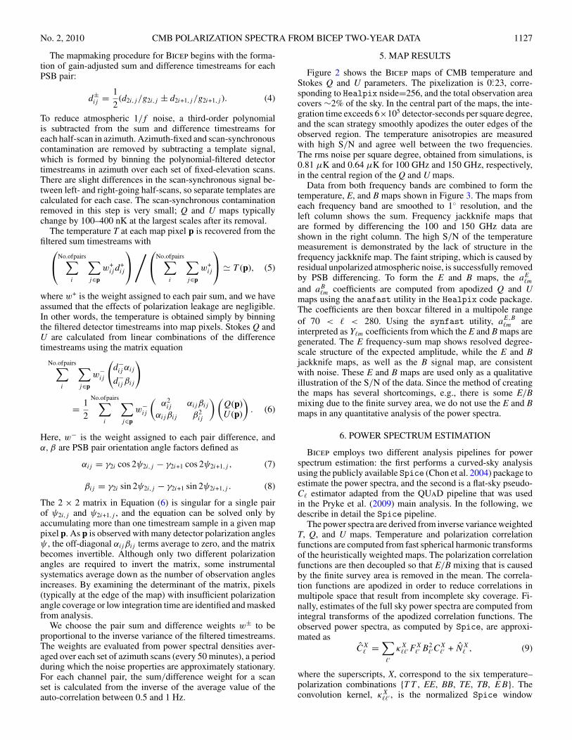
5. MAP RESULTS

Figure 2 shows the Bicep maps of CMB temperature andStokes Q and U parameters. The pixelization is 0.◦23, corre-sponding to Healpix nside=256, and the total observation areacovers ∼2% of the sky. In the central part of the maps, the inte-gration time exceeds 6×105 detector-seconds per square degree,and the scan strategy smoothly apodizes the outer edges of theobserved region. The temperature anisotropies are measuredwith high S/N and agree well between the two frequencies.The rms noise per square degree, obtained from simulations, is0.81 μK and 0.64 μK for 100 GHz and 150 GHz, respectively,in the central region of the Q and U maps.

Data from both frequency bands are combined to form thetemperature, E, and B maps shown in Figure 3. The maps fromeach frequency band are smoothed to 1◦ resolution, and theleft column shows the sum. Frequency jackknife maps thatare formed by differencing the 100 and 150 GHz data areshown in the right column. The high S/N of the temperaturemeasurement is demonstrated by the lack of structure in thefrequency jackknife map. The faint striping, which is caused byresidual unpolarized atmospheric noise, is successfully removedby PSB differencing. To form the E and B maps, the aE

�m

and aB�m coefficients are computed from apodized Q and U

maps using the anafast utility in the Healpix code package.The coefficients are then boxcar filtered in a multipole rangeof 70 < � < 280. Using the synfast utility, a

E,B�m are

interpreted as Y�m coefficients from which the E and B maps aregenerated. The E frequency-sum map shows resolved degree-scale structure of the expected amplitude, while the E and Bjackknife maps, as well as the B signal map, are consistentwith noise. These E and B maps are used only as a qualitativeillustration of the S/N of the data. Since the method of creatingthe maps has several shortcomings, e.g., there is some E/Bmixing due to the finite survey area, we do not use the E and Bmaps in any quantitative analysis of the power spectra.

6. POWER SPECTRUM ESTIMATION

Bicep employs two different analysis pipelines for powerspectrum estimation: the first performs a curved-sky analysisusing the publicly available Spice (Chon et al. 2004) package toestimate the power spectra, and the second is a flat-sky pseudo-C� estimator adapted from the QUaD pipeline that was usedin the Pryke et al. (2009) main analysis. In the following, wedescribe in detail the Spice pipeline.

The power spectra are derived from inverse variance weightedT, Q, and U maps. Temperature and polarization correlationfunctions are computed from fast spherical harmonic transformsof the heuristically weighted maps. The polarization correlationfunctions are then decoupled so that E/B mixing that is causedby the finite survey area is removed in the mean. The correla-tion functions are apodized in order to reduce correlations inmultipole space that result from incomplete sky coverage. Fi-nally, estimates of the full sky power spectra are computed fromintegral transforms of the apodized correlation functions. Theobserved power spectra, as computed by Spice, are approxi-mated as

CX� =

∑�′

κX��′F

X�′ B

2�′C

X�′ + NX

� , (9)

where the superscripts, X, correspond to the six temperature–polarization combinations {T T , EE, BB, TE, TB, EB}. Theconvolution kernel, κX

��′ , is the normalized Spice window

1128 CHIANG ET AL. Vol. 711

Figure 2. Bicep T, Q, U, and coverage maps. The resolution is about 0.◦9 and 0.◦6 at 100 and 150 GHz, respectively, and no smoothing or apodizing has been appliedto the maps. The noise per square degree in the central region of the Q and U maps is 0.81 μK at 100 GHz and 0.64 μK at 150 GHz. Note that the color scales of thetemperature and polarization maps differ by a factor of 10.

function and depends on the apodization function applied tothe correlation functions. The effect of timestream filtering isdescribed by FX

� , the �-space transfer function; B2� = B2

� H2�

is the product of the beam and pixel window functions, andNX

� is the power spectrum of the noise convolved with theSpice kernel. In the following subsections, we describe thesteps in solving Equation (9) and recovering an estimate ofthe underlying power spectrum, CX

� .

6.1. Noise Subtraction

The first step in power spectrum estimation is calculating andsubtracting the noise bias N�. We estimate N� with Monte Carlosimulations of instrument noise: starting from a noise model,we generate simulated timestreams that are filtered, co-addedinto maps, and processed with Spice. The resulting simulatednoise spectra are averaged over many realizations to form N�.

The Bicep noise model is derived from gain-adjusted PSBpair sum and difference timestreams (Equation (4)) under the

assumption that the timestream S/N is negligible, i.e., thesignal is the noise. The S/N is � 10% and � 0.1% forthe sum and difference timestreams, respectively. The sumand difference timestreams are polynomial-filtered and Fouriertransformed over each half-scan, and all auto-correlations andcross-correlations between channel pairs are computed to formthe complex frequency-domain noise covariance matrix N(f ).To form the noise model, we average N(f ) over the 100half-scans within each scan set and then average into 12logarithmically spaced bins spanning 0.05–5 Hz.

To construct simulated correlated noise timestreams, we takethe Cholesky decomposition N(f ) = L(f )L†(f ) of the noisecovariance matrix and multiply a vector of pseudo-randomcomplex numbers ρ(f ) by L(f ):

v(f ) = L(f )ρ(f ). (10)

The complex numbers in ρ(f ) have Gaussian-distributed realand imaginary components and are normalized such that themagnitude has a standard deviation of one. The resulting product

No. 2, 2010 CMB POLARIZATION SPECTRA FROM BICEP TWO-YEAR DATA 1129

Figure 3. Data from Bicep’s 100 GHz and 150 GHz channels are combined to form temperature, E, and B signal and jackknife maps. The E and B maps are apodizedto downweight noise-dominated edge pixels. The temperature anisotropies are measured with high S/N, and the E signal map shows resolved degree-scale structure.The B signal map and the E and B jackknife maps are consistent with noise.

v(f ) has the same statistical properties as the data and isinverse Fourier transformed to obtain a set of simulated noisetimestreams. Scan-synchronous templates are calculated andsubtracted from each set of azimuth scans, and the filtered noisetimestreams are then co-added into maps.

The noise bias, N�, is estimated by averaging the power spec-tra from an ensemble of noise-only maps. Figure 4 shows N�

(red dashed lines), calculated from the average over 500 real-izations, in comparison to raw power spectra. Bicep measuresTT and TE with high S/N, and the noise contribution is negli-gible up to � ∼ 330. The noise is mostly uncorrelated betweentemperature and polarization, so N� for TB is distributed aroundzero, and the same is true for EB. In contrast, noise comprisesthe bulk of the EE and all of the BB amplitude at � > 150,which illustrates the need for careful noise modeling and sub-traction. We have studied the impact of noise misestimation byintentionally scaling the noise spectra (Takahashi et al. 2010),and we find that the largest possible error in N� is ±3%.

6.2. Beam and Pixelization Corrections

The finite resolution of the telescope and pixelization of themaps result in suppression of the observed power spectra atsmall angular scales. This suppression of power is describedby B2

� = B2� H

2� , the product of the beam and pixel window

functions, and is illustrated in Figure 5. In this analysis, weapproximate B� as the Legendre transform of the average beamwithin a given frequency band, which is assumed to be a circularGaussian. The full widths at 100 and 150 GHz are 0.◦93 and

0.◦60, respectively. The pixel window function H� is supplied byHealpix and corresponds to nside=256. In the case of Bicep,B� varies slowly with respect to the Spice kernel, κX

��′ , and cantherefore be pulled out of the convolution. The observed powerspectra, after noise subtraction, are divided by B2

� to correct forthe effects of beam suppression and pixelization:

(CX

� − NX�

)/B2

� �∑�′

κX��′F

X�′ C

X�′ . (11)

6.3. Filter Corrections

The bolometer timestreams are cleaned by subtracting a third-order polynomial and scan-synchronous template; this cleaningprocedure also has the effect of removing large-scale CMBsignal. The amount of signal loss is described by F�, the �-spacetransfer function imposed by timestream filtering. In addition,although the Spice estimator is unbiased in the mean, thetimestream processing removes spatial modes from the observedT, Q, and U maps, generically introducing couplings betweenthe observed E and B spectra. These couplings are small, but areof interest for the leakage of the relatively large E-mode signalinto B-mode polarization. We characterize both F� and E-to-Bleakage with signal-only simulations.

The signal simulation procedure begins by generating modelpower spectra using the CAMB (Lewis et al. 2000) softwarepackage. We use ΛCDM parameters derived from WMAP five-year data (Hinshaw et al. 2009) and a tensor-to-scalar ratioof zero. From the model spectra, we use the synfast utility

1130 CHIANG ET AL. Vol. 711

0

2000

4000

6000

l(l+

1)C

l / 2

π (

μK2 )

0

10

20

-100

0

100

0

10

20

-20

0

20

0 100 200 300-2

-1

0

1

2

0 100 200 300

l

EETT

BBET

BEBT

Multipole

Figure 4. Raw power spectra, uncorrected for noise and filter bias, are shown here for 500 signal-plus-noise simulations (gray lines) and Bicep 150 GHz data (blackpoints). The dashed red lines indicate the level of noise bias, �(� + 1)N�/(2π ), and the black lines show the ΛCDM spectra used as inputs for the signal simulations.Noise dominates much of the EE spectrum and all of the BB spectrum. The effect of filter bias is visible in the low-� portion of the TT spectrum, where the simulatedspectra fall below the model curve.

0

0.1

0.2

0.3

0.4

0.5

0.6

0.7

0.8

0.9

1

0 50 100 150 200 250 300

l

Fil

ter

an

d b

ea

m f

un

cti

on

s

TT

TE, TB

EE, BB, EB

150 GHz

100 GHz

Multipole

Figure 5. Signal-only simulations are used to evaluate the filter function FXb ,

shown here for 150 GHz (FXb for other frequency combinations look similar).

The beam–pixel window functions B2� = B2

� H 2� are shown for 100 and 150 GHz.

in Healpix to create an ensemble of simulated CMB skiespixelized at 0.◦11 resolution (nside=512) and convolved with theBicep beams. Actual pointing data are used to generate smoothlyinterpolated PSB timestreams from the simulated T ,Q,U mapsand their derivatives. A PSB timestream sample d(p) that fallsinto a pixel centered at p is expressed as a convolution of thebeam P (r − rb), which is centered at rb, with a second-orderTaylor expansion of the sky signal m around p (E. F. Hivon &N. Ponthieu 2010, in preparation):

d(p) =∫

dr P (r − rb)[m(p) + ∇m(p)(r − p)

+1

2(r − p)T D2m(p)(r − p)

]. (12)

Here, m(p) = g[T (p) + γ (Q(p) cos 2ψ + U (p) sin 2ψ)], and∇ and D2 denote the first and second derivatives in spherical

coordinates. Assuming Gaussian beams for each frequencyband, Equation (12) reduces to

d(p) = m(p) + ∇m(p)(rb − p)

+1

2Tr

[D2m(p)

((Δφ)2 ΔφΔθ

ΔφΔθ (Δθ )2

) ], (13)

where Δφ and Δθ are the longitude and latitude offsets be-tween the pointing vector rb and the pixel center p. We applyEquation (13) to simulate signal-only detector timestreams ac-cording to Bicep’s scan strategy. Measured PSB pair centroids,detector orientation angles, and cross-polar leakage values areincluded in the simulations. For the purpose of characterizingthe effects of timestream filtering, all differential beam system-atic effects are turned off so that there is no mixing betweentemperature and polarization. The simulated timestreams arefiltered and weighted in exactly the same way as the real dataand then co-added into maps.

Once we have “Bicep-observed” signal-only maps in hand,we compute the power spectra with Spice and average theresults over many realizations. Because the input CAMB spectrahave r = 0, any non-zero BB power in the simulation outputs isinterpreted as contamination from E-mode polarization that isinduced by timestream filtering. We therefore apply a correction,

(CBB

� − NBB� − CBB

� |EEonly)/B2

� �∑�′

κBB��′ FBB

�′ CBB�′ , (14)

to the BB power spectrum of the data, where CBB� |EEonly is the

ensemble average BB spectrum from the r = 0 signal simulationoutputs. The amplitude of this correction is roughly �(� +1)CBB

� |EEonly/(2π ) � 3 × 10−3μK2 at � ∼ 100, comparableto inflationary BB power for r = 0.05, and the sample varianceis about 3×10−3μK2. The correction factors for the other spectraare negligibly small, so only the BB spectrum is adjusted withthis procedure.

No. 2, 2010 CMB POLARIZATION SPECTRA FROM BICEP TWO-YEAR DATA 1131

To quantify the suppression of large-scale power fromtimestream filtering, we begin by assuming that FX

� , like B2� ,

varies slowly in comparison to the Spice kernel and can bepulled out of the convolution. We choose to calculate the binnedfilter suppression factor, FX

b , defined as

∑�

P b�

�(� + 1)

2π

(CX

� − NX�

)B2

�

� FXb

∑�

P b�

�(� + 1)

2π

∑�′

κ��′CX�′ ,

(15)where the binning operator P b

� is a top hat. (In the caseof the BB spectrum, the left hand side of the equation alsocontains CBB

� |EEonly, as in Equation (14).) We obtain the filtersuppression factors by comparing the power spectra of theBicep-observed signal-only maps to those of the input synfastmaps; FX

b is the ratio of the spectra, after multiplying by�(� + 1)/(2π ) and binning.

Figure 5 shows FXb averaged over 500 signal simulations

using Bicep’s timestream filtering. In each simulation, signal-only timestreams are generated from the full two years ofpointing data. At � ∼ 100, the value of FX

b is about 0.7 for allspectra and rises slowly as � increases. Identical filter functionsare used for the EE and BB spectra, and the filter functionsof the cross-spectra are calculated as the geometric mean ofthose determined from the auto-spectra. The validity of thisapproach for obtaining the BB and cross-spectra filter functionshas been confirmed with simulations over a limited multipolerange. Dividing by FX

b is the final step in obtaining the Bicep

band power estimates:

CX

b ≡ 1

FXb

∑�

P b�

�(� + 1)

2π

(CX

� − NX�

)B2

�

, X �= BB (16)

CBB

b ≡ 1

FBBb

∑�

P b�

�(� + 1)

2π

(CBB

� − NBB� − CBB

� |EEonly)

B2�

.

(17)

6.4. Error Bars

The uncertainties in the power spectra consist of two compo-nents, one that is proportional to the signal itself (sample vari-ance), and another that depends on the instrumental noise. Weestimate the errors by examining the variance of power spectrafrom simulated signal-plus-noise maps, which exactly encodetime-dependent correlated noise, scan strategy, and sky cover-age. We add the simulated noise-only and signal-only maps,described in Sections 6.1 and 6.3; and power spectra are cal-culated for each realization using the same N�, B2

� , and FXb as

applied to the real data. If the simulations include a reasonablemodel of the signal and faithfully reproduce all the noise prop-erties of the experiment, then the data and simulations shouldbe indistinguishable. Figure 4 shows raw power spectra, un-corrected for noise and filter bias, from 500 signal-plus-noisesimulations at 150 GHz. The raw spectra of the actual data,shown by the black points, lie within the scatter of the simula-tions. We calculate the band power covariance matrix from theensemble of simulations, after applying noise, filter, and beamcorrections. The band power errors are obtained from squareroot of the diagonal terms of the matrix.

6.5. Band Power Window Functions

In order to compare our band power estimates to a theoreticalmodel, we need a method to calculate expected band power

values from theoretical power spectra. The relationship betweenthe model and the expected band powers is described by bandpower window functions, ωb

� , defined as

Cb =∑

�

(� + 12 )

�(� + 1

)ωb�C�, (18)

where C� ≡ �(� + 1)C�/(2π ). The window functions are givenby

ωb� = 2

2� + 1

∑�′

P b�′�

′(�′ + 1)κ�′� (19)

and are normalized such that∑�

(� + 12 )

�(� + 1)ωb

� = 1. (20)

The window functions depend on the Spice kernel, whichdepends on the apodization function applied to the correlationfunctions. For this analysis, we apodize the correlation functionswith a cosine window that spans 50◦. We choose to use auniform binning of width Δ� = 35, spanning a multipole rangeof 21 � � � 335. This choice of bin width provides minimallycorrelated band powers while preserving the spectral resolutiondetermined by the width of the Spice kernel. Figure 6 illustratesBicep’s band power window functions for the nine � bins.

Because the BB power spectrum is debiased with the proce-dure described in Equation (14), we set the EE-to-BB windowfunctions to zero. This is a valid approximation as long as the EEspectrum of the signal under consideration is statistically con-sistent with the measured Bicep band powers (which, as shownin Section 12, are well described by a concordance ΛCDM cos-mology).

7. POWER SPECTRUM RESULTS

Figure 7 shows the full set of Bicep spectra plotted with aΛCDM model derived from WMAP five-year data. The 100 and150 GHz auto-spectra are shown, as well as the 100 × 150 cross-spectra. In the case of the TE, TB, and EB spectra, we also showthe 150×100 cross-correlation. For each spectrum, we presentnine band powers with a uniform bin width of Δ� = 35, spanning21 � � � 335. The TT , TE, and EE spectra are detected withhigh significance and are already sample-variance limited, andthere is no detection of signal in BB, TB, and EB. The resultsfrom Bicep’s two analysis pipelines agree well with each other,and Figure 11 shows a comparison of the frequency-combinedpower spectra (Section 11).

As a cross-check, we have also derived TT , TE, and TBspectra using WMAP five-year temperature data in Bicep’s CMBfield (open circles in Figure 7). The WMAP temperature mapsare smoothed and filtered identically to Bicep, as describedin Section 3.2. The TT points are calculated from the cross-correlation of the WMAP Q- and V-band maps, and the TEand TB spectra are calculated using WMAP V-band temperaturedata and Bicep polarization data. For this comparison, we donot subtract noise bias and instead rely on the fact that thepairs of maps have uncorrelated noise. We also do not attemptto assign error bars. Qualitatively, the spectra formed usingWMAP temperature data agree well with the spectra from Bicep

temperature and polarization data. Both the Bicep and WMAPtemperature maps are strongly signal-dominated; apparentlythe differences between them, including the noise as well aspotential systematics, are at a level that has little impact on theTT , TE, or TB power spectra results.

1132 CHIANG ET AL. Vol. 711

0

0.01

0.02

0.03

TT

0

0.01

0.02

0.03

TE

, T

B

0

0.01

0.02

0.03

0 50 100 150 200 250 300 350

EE

, B

B, E

B

lMultipole

Figure 6. Bicep’s band power window functions are defined by Equation (18), and this figure shows ωb�/�.

8. CONSISTENCY TESTS

8.1. Jackknife Descriptions

We check the self-consistency of the power spectra byperforming jackknives, statistical tests in which the data aresplit in two halves and differenced. The split is performedat the mapmaking stage, and the resulting differenced mapshould have power spectra that are consistent with the expectedresidual signal level (nearly zero) after subtracting noise bias.The interaction of timestream filtering with the details of the splitcauses imperfect signal cancellation when forming jackknifemaps, but in practice, this residual signal is small.

The data are tested with six jackknives that are sensitive todifferent aspects of the instrument’s performance. In the scandirection jackknife, the data are split into left- and right-goingazimuth half-scans. Failures generally point to a problem in thedetector transfer function deconvolution, or thermal instabilitiescreated at the scan endpoints. The elevation coverage jackknifeis formed from the two CMB observations in each 48 hr cycle;each observation covers the same azimuth range but starts froma different elevation. This jackknife is sensitive to ground-fixed or scan-synchronous contamination. Bicep observes atfour fixed boresight orientation angles that can be split intotwo pairs, {−45◦, 0◦} and {135◦, 180◦}, to form a boresightangle pair jackknife. This test is perhaps the most powerfulof the jackknives performed and is sensitive to many factors,including thermal stability, atmospheric opacity, relative gainmismatches, differential beam pointing, and ground pickup.In the temporal jackknife, the 8 day observing cycles—48 hrat each of the four boresight angles—are interleaved to formthe two halves, and this jackknife tests sensitivity to weather

changes. The season split jackknife simply divides the datainto the two observing seasons, and failures reflect any changesmade to the instrument between the two years. In particular,the focal plane thermal architecture was improved for the 2007season, and the temperature control scheme was changed. Thefocal plane QU jackknife splits the detectors into two groupsaccording to their polarization orientation within the focal plane(approximately alternating hextants) and is a method of probinginstrumental polarization effects.

Power spectra of jackknife maps are computed with themethod described in Section 6, using simulated jackknifenoise and signal-plus-noise maps to subtract noise bias andassign error bars. The filter function FX

b is applied so thatthe magnitude of any non-zero jackknife band powers canbe compared to the amplitude of the non-jackknife spectra.For each jackknife spectrum, we calculate χ2 over nine binsspanning 21 � � � 335. To account for the expected levelof residual signal, the χ2 values are evaluated with respect tothe average jackknife spectra from an ensemble of signal-onlysimulations. The criteria for jackknife success or failure arebased on the probability to exceed (PTE) the χ2 value, whichis calculated from the distribution of χ2 in 500 signal-plus-noise simulations. Jackknife victory is declared when (1) noneof the PTEs are abnormally high or low, given the number of χ2

tests performed, and (2) the PTEs are consistent with a uniformdistribution between zero and one.

8.2. Jackknife Results

The jackknife spectra for the six different data splits appearsimilar in that the band powers are all distributed around

No. 2, 2010 CMB POLARIZATION SPECTRA FROM BICEP TWO-YEAR DATA 1133

0

5000

TT

100 GHz auto 150 GHz auto 100 x 150 GHz 150 x 100 GHz

0

200

TE

-50

0

50

TB

0

2

EE

-2

0

2

BB

-2

0

2

0 200

EB

0 200 0 200 0 200

Figure 7. Black points show the full set of Bicep’s power spectra. The horizontal axis is multipole moment �, and the vertical axis is �(� + 1)C�/(2π ) in units ofμK2. The spectra agree well with a ΛCDM model (black lines) derived from WMAP five-year data and r = 0. The gray points correspond to the boresight anglepair jackknife; note that although the TT , TE, and TB jackknife failures are statistically significant, the amplitudes are small compared to the signal. The open circlesshow spectra calculated using WMAP five-year temperature data, smoothed and filtered identically to Bicep. We have cross-correlated the WMAP Q- and V-band datain Bicep’s CMB field to obtain the TT points, and the TE and TB spectra are calculated from the cross-correlation of WMAP V-band temperature data with Bicep

polarization data.

0

1

2

3

4

5

6

7

8

9

10

0 0.1 0.2 0.3 0.4 0.5 0.6 0.7 0.8 0.9 1

EE, BB, EB jackknife PTE

Co

un

ts

Figure 8. Probabilities to exceed the χ2 values from EE, BB, and EB jackknife tests are consistent with a uniform distribution between zero and one.

zero. We therefore show only the spectra from the boresightpair jackknife (Figure 7, gray points), which is arguably themost stringent of the six tests. Table 1 lists the PTE values

from all of the jackknife χ2 tests for Bicep’s polarization-onlyspectra (EE,BB,EB). Out of all the PTEs, the lowest valueis 0.014, in the 150 GHz focal plane QU jackknife. This low

1134 CHIANG ET AL. Vol. 711

Table 1Jackknife PTE Values from χ2 Tests

Jackknife 100 GHz 150 GHz 100 × 150 150 × 100

Scan directionEE 0.532 0.588 0.740BB 0.640 0.568 0.212EB 0.816 0.962 0.924 0.358

Elevation coverageEE 0.576 0.546 0.924BB 0.584 0.288 0.618EB 0.872 0.728 0.892 0.892

Boresight angleEE 0.916 0.448 0.320BB 0.242 0.548 0.592EB 0.912 0.100 0.392 0.944

Temporal splitEE 0.378 0.208 0.796BB 0.788 0.020 0.852EB 0.370 0.580 0.476 0.232

Season splitEE 0.564 0.716 0.216BB 0.790 0.992 0.056EB 0.806 0.514 0.456 0.986

Focal plane QU

EE 0.670 0.014 0.994BB 0.896 0.804 0.576EB 0.236 0.806 0.234 0.560

value is, however, consistent with expectations from uniformlydistributed PTEs over the 60 polarization-only jackknives.Figure 8 shows that the PTEs are consistent with a uniformdistribution between zero and one.

The polarization jackknife tests are the most powerful probeof the accuracy of the noise model. In addition to the χ2 tests,we have also expressed the jackknife spectra as band powerdeviations with respect to the mean of signal-only simulations.The sum of the band power deviations in each jackknifespectrum provides an additional and more precise gauge of thecorrect estimation of instrument noise. We have verified that theband power deviation sums in the data are consistent with signal-plus-noise simulations and are not systematically biased high orlow, thus confirming that the noise levels are correctly estimated.Furthermore, we have probed the sensitivity to systematicvariations in the modeled noise amplitude over a range that iscomparable to the S/N of the sum and difference timestreams,and find no significant changes in the jackknife spectra. Therelative insensitivity of the jackknifes to the amplitude of thenoise model validates the procedure described in Section 6.1.

In contrast to the polarization data, the temperature datadisplay significant jackknife failures. There is an excess of smallPTE values in the TE and TB jackknives, and most of the TTjackknife PTEs are smaller than 0.002, which is the resolutionfrom 500 simulations. The TT , TE, and TB jackknife PTEs aretherefore not listed in Table 1. We attribute these failures tothe fact that Bicep’s temperature maps have high S/N (see TTplot in Figure 4), and the jackknives are therefore extremelysensitive to small gain calibration errors or imperfections inmodeling and subtracting unpolarized atmospheric emission.(As described in Section 6.1, the �10% S/N in the pair-sumtimestreams is a known imperfection of the Bicep noise modelfor temperature data.) Although the TT , TE, and TB jackknifefailures are statistically significant, Figure 7 illustrates that the

amplitudes of the jackknife spectra are small compared to boththe amplitude and errors of the signal spectra. The magnitudesof the TT and TE/TB jackknife band powers are typically1–10 μK2 and 0.1–1 μK2, respectively. In all cases, the errorbars of the non-jackknife spectra are at least a factor of 10 larger,except in the highest � bin.

We have performed the same jackknives with both analysispipelines, and the results are in excellent agreement. Thealternate pipeline confirms that the polarization data pass theχ2 tests, and although the TT , TE, and TB spectra do not pass,the amplitudes of the jackknife spectra are small.

9. SYSTEMATIC UNCERTAINTIES

Systematic errors that arise from uncertainties in instrumentcharacterization can be separated into two categories: (1) errorsthat mix temperature, E-mode, and B-mode polarization; and (2)calibration uncertainties that affect only the scaling or amplitudeof the spectra. In this section, we describe the dominant sourcesof systematic error in Bicep and the expected impact on thepower spectra; these systematics are summarized in Figure 9.A complete description of all potential Bicep systematics andthe methodology for propagating the errors to the power spectrais given in the accompanying instrument characterization paper(Takahashi et al. 2010).

9.1. Temperature and Polarization Mixing

We are mostly concerned with systematic errors that mixthe bright temperature signal into polarization and thus induce afalse B-mode signal. We define a benchmark for each systematicerror such that the false B-mode amplitude is no greater thanthe peak of the inflationary BB spectrum. For Bicep’s target ofr = 0.1, this requirement corresponds to �(� + 1)CBB

� /(2π ) =7 × 10−3μK2 at � ∼ 100.

The primary source of potential temperature leakage into po-larization is differential gains within PSB pairs. Gain mismatcheffects can also arise from other systematics, such as errors in thebolometer transfer functions, which act as frequency-dependentgains. We have characterized the common-mode rejection ofPSBs by examining the cross-correlation of pair-sum and pair-difference maps. There is no statistically significant evidencefor gain mismatch in the data, and we set an upper limit ofΔ(g1/g2)/(g1/g2) < 1.1% on differential gains.

A second source of potential temperature and polarizationmixing is beam mismatch within PSB pairs. We describe beammismatch with three quantities: differential beam size, pointing,and ellipticity. Of these three, the dominant effect in Bicep isdifferential pointing, which is stable over time and has beenmeasured with a median amplitude of (r1−r2)/σ = 1.3 ± 0.4%,where σ is the average Gaussian beam size within a pair ofPSBs. Measured upper limits on differential size and ellipticityare negligible.

Most systematic errors interact with the scan strategy incomplex ways, and the exact effects on the power spectra canbe computed only through signal simulations. We follow theformalism presented in E. F. Hivon & N. Ponthieu (2010, inpreparation) and Shimon et al. (2008) to calculate the expectedlevel of false BB in Bicep. Starting from synfast maps withr = 0, Equation (13) is used to generate simulated signaltimestreams that include the effects of gain mismatch anddifferential pointing. The timestreams are filtered and co-addedinto maps, and the amplitude of the BB power spectrum at� ∼ 100 is compared with the 7 × 10−3μK2 benchmark.

No. 2, 2010 CMB POLARIZATION SPECTRA FROM BICEP TWO-YEAR DATA 1135

10-1

1

10

102

10 3

TT

100 GHz auto 150 GHz auto

10-1

1

10

TE

10-3

10-2

10-1

1

EE

10-3

10-2

10-1

1

0 100 200 300

BB

0 100 200 300

Total randomSampleNoise

Abs cal sysBeam sys

Gain mismatchDiff pointing

Figure 9. Dominant systematic uncertainties in Bicep’s band powers are compared to the total statistical error, which comes from sample variance and noise. Thehorizontal axis is multipole moment �, and the vertical axis is �(� + 1)C�/(2π ) uncertainty in units of μK2. The contributions from the signal–noise cross terms to thetotal statistical error in TE are not shown. We have assumed that gain mismatch and differential pointing systematics leak temperature to EE and BB in equal amounts.

In the differential gain simulations, we randomly assign 1.1%rms gain mismatch to PSB pairs, and we find that the expectedfalse BB amplitude is 7.4 × 10−3μK2 and 2.9 × 10−2μK2 at� ∼ 100 for 100 and 150 GHz, respectively. Although thisamplitude exceeds the r = 0.1 benchmark, Figure 9 illustratesthat it is small compared to the statistical error in this analysis ofthe two-year data. In a future analysis of the entire Bicep data set,we anticipate placing tighter constraints on PSB gain mismatchas the noise levels integrate down. With further work, we areconfident that uncertainty in gain mismatch can be substantiallyreduced from the current 1.1%.

Differential pointing has been precisely characterized foreach of Bicep’s PSB pairs, so we run signal simulations usingthe measured centroid offset vectors, rather than randomizeddistributions. The false BB from differential pointing has an� ∼ 100 amplitude of 2.7 × 10−3μK2 and 4.2 × 10−3μK2 at100 and 150 GHz, respectively. These amplitudes are slightlysmaller than the r = 0.1 benchmark and are well below thenoise level of the initial two-year data set. In a future analysis, itmay be possible to use the measured centroid offsets to correctfor systematic effects.

We emphasize that, in addition to the differential gainand pointing discussed here, most uncertainties in instrumentcharacterization create false positive BB signal. The fact thatBicep’s BB spectra are consistent with zero and pass jackknivesdemonstrates that we have achieved sufficient control oversystematic errors in this analysis. Furthermore, until a positiveB-mode detection is made, the presence of systematic effectsthat produce spurious polarization could only make the reportedBB upper limits higher (more conservative) than they would beotherwise.

9.2. Absolute Gain and Beam Uncertainty

The scaling of the power spectra is determined by the absolutegain factors that convert detector units to temperature, and the2% uncertainty in this gain (Section 3.2) translates into a 4% un-certainty in the power spectrum amplitude. The polarized spectrahave additional amplitude uncertainty that arises from errors inthe cross-polar leakage. A systematic error of Δε = 0.01 cor-responds to 3.9% amplitude uncertainty for polarization-onlyspectra (EE, BB, EB) and 2.0% for temperature–polarization

1136 CHIANG ET AL. Vol. 711

cross-spectra (TE, TB). Therefore, the combined amplitude un-certainty GX ≡ ΔCX

� /CX� from gain and ε errors is 4% for TT ,

4.5% for TE/TB, and 5.6% for EE/BB/EB. These uncertaintiesare shown in Figure 9, assuming ΛCDM spectra with r = 0.

For Gaussian beams, measurement errors in the beam widthsintroduce a fractional uncertainty,

S� ≡ ΔCX�

/CX

� = eσ 2�(�+1)(δ2+2δ) − 1 − S, (21)

in the power spectrum amplitude as a function of �. Here,σ = FWHM/

√8 ln(2), and δ is the fractional beam width error

Δσ/σ . Because this band power uncertainty is degenerate withabsolute gain error, we subtract the mean, S, calculated over56 � � � 265, the angular scales over which we perform abso-lute calibration. For this analysis, we use average beam widthsof 0.◦93 and 0.◦60 at 100 and 150 GHz, respectively. Although thedistribution of beam widths in the focal plane varies by ±3%,the measurement precision is ±0.5%; we therefore expect theeffective δ to lie somewhere in between. We calculate the maxi-mum beam width error allowed by our calibration cross-spectra(Equation (2)), which are very close to flat, and we constrainδ < 1.2% and δ < 2.8% at 100 and 150 GHz, respectively.Figure 9 shows the expected power spectrum errors from thesemaximum allowed beam uncertainties, which are most likelyconservative. The systematic error is smaller than the statisticalerror in all cases except the TT spectra at high �, where the levelsof statistical and beam systematic uncertainty are comparable.

10. FOREGROUNDS

The Bicep CMB region was chosen to have the lowestforeground dust emission for a field of that size, and we donot expect foreground contamination from dust or other sourcesto be significant at the current depth in the maps. To verify this,we estimate the levels of contamination in Bicep CMB datafrom three potential foreground sources: thermal dust emission,synchrotron radiation, and extragalactic radio point sources.

10.1. Thermal Dust

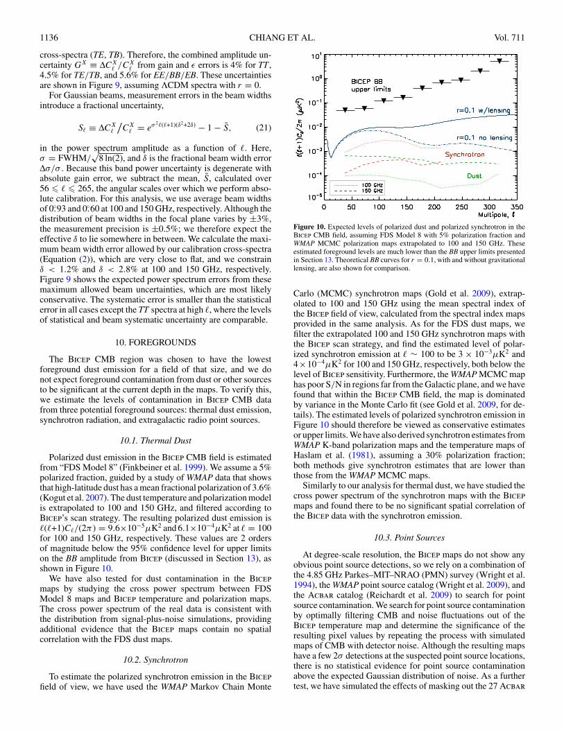
Polarized dust emission in the Bicep CMB field is estimatedfrom “FDS Model 8” (Finkbeiner et al. 1999). We assume a 5%polarized fraction, guided by a study of WMAP data that showsthat high-latitude dust has a mean fractional polarization of 3.6%(Kogut et al. 2007). The dust temperature and polarization modelis extrapolated to 100 and 150 GHz, and filtered according toBicep’s scan strategy. The resulting polarized dust emission is�(�+1)C�/(2π ) = 9.6×10−5μK2 and 6.1×10−4μK2 at � = 100for 100 and 150 GHz, respectively. These values are 2 ordersof magnitude below the 95% confidence level for upper limitson the BB amplitude from Bicep (discussed in Section 13), asshown in Figure 10.

We have also tested for dust contamination in the Bicep

maps by studying the cross power spectrum between FDSModel 8 maps and Bicep temperature and polarization maps.The cross power spectrum of the real data is consistent withthe distribution from signal-plus-noise simulations, providingadditional evidence that the Bicep maps contain no spatialcorrelation with the FDS dust maps.

10.2. Synchrotron

To estimate the polarized synchrotron emission in the Bicep

field of view, we have used the WMAP Markov Chain Monte

Figure 10. Expected levels of polarized dust and polarized synchrotron in theBicep CMB field, assuming FDS Model 8 with 5% polarization fraction andWMAP MCMC polarization maps extrapolated to 100 and 150 GHz. Theseestimated foreground levels are much lower than the BB upper limits presentedin Section 13. Theoretical BB curves for r = 0.1, with and without gravitationallensing, are also shown for comparison.

Carlo (MCMC) synchrotron maps (Gold et al. 2009), extrap-olated to 100 and 150 GHz using the mean spectral index ofthe Bicep field of view, calculated from the spectral index mapsprovided in the same analysis. As for the FDS dust maps, wefilter the extrapolated 100 and 150 GHz synchrotron maps withthe Bicep scan strategy, and find the estimated level of polar-ized synchrotron emission at � ∼ 100 to be 3 × 10−3μK2 and4×10−4μK2 for 100 and 150 GHz, respectively, both below thelevel of Bicep sensitivity. Furthermore, the WMAP MCMC maphas poor S/N in regions far from the Galactic plane, and we havefound that within the Bicep CMB field, the map is dominatedby variance in the Monte Carlo fit (see Gold et al. 2009, for de-tails). The estimated levels of polarized synchrotron emission inFigure 10 should therefore be viewed as conservative estimatesor upper limits. We have also derived synchrotron estimates fromWMAP K-band polarization maps and the temperature maps ofHaslam et al. (1981), assuming a 30% polarization fraction;both methods give synchrotron estimates that are lower thanthose from the WMAP MCMC maps.

Similarly to our analysis for thermal dust, we have studied thecross power spectrum of the synchrotron maps with the Bicep

maps and found there to be no significant spatial correlation ofthe Bicep data with the synchrotron emission.

10.3. Point Sources

At degree-scale resolution, the Bicep maps do not show anyobvious point source detections, so we rely on a combination ofthe 4.85 GHz Parkes–MIT–NRAO (PMN) survey (Wright et al.1994), the WMAP point source catalog (Wright et al. 2009), andthe Acbar catalog (Reichardt et al. 2009) to search for pointsource contamination. We search for point source contaminationby optimally filtering CMB and noise fluctuations out of theBicep temperature map and determine the significance of theresulting pixel values by repeating the process with simulatedmaps of CMB with detector noise. Although the resulting mapshave a few 2σ detections at the suspected point source locations,there is no statistical evidence for point source contaminationabove the expected Gaussian distribution of noise. As a furthertest, we have simulated the effects of masking out the 27 Acbar

No. 2, 2010 CMB POLARIZATION SPECTRA FROM BICEP TWO-YEAR DATA 1137

sources that lie within the Bicep field and have found it has nosignificant impact on the power spectra.

10.4. Frequency Jackknife

The CMB and foreground emission have different frequencydependence, so we can test for the presence of foreground con-tamination in Bicep data by performing a frequency jackknife.We difference the 100 and 150 GHz maps, compute the powerspectra, calculate χ2, and compare the results to signal-plus-noise simulations, as described in Section 8.1. The probabilitiesto exceed the χ2 values are {0.050, 0.152, 0.732} for EE, BB,and EB, respectively. We find no evidence for foreground con-tamination in the frequency jackknives.

11. COMBINED SPECTRA

We combine the spectra from the different observing frequen-cies by taking a weighted average for each band power. To obtainthe weights, we use signal-plus-noise simulations to calculatethe covariance matrices from the various frequency combina-tions (100, 150, 100 × 150, and 150 × 100 GHz). There arethree unique combinations for TT , EE, and BB, and four combi-nations for the other spectra. The weights are calculated from therow/column sums of the inverse of the covariance matrices. Theerror bars of the combined spectra are determined by applyingthe same combination weights to signal-plus-noise simulations.For fully noise-dominated spectra (such as BB), the error barsof the combined spectra improve by 10%–40% compared to theerrors from 150 GHz data alone.

As suggested by Bond et al. (2000), we apply a transformation

Zb = ln(Cb + xb) (22)

to account for the fact that the probability of the true model value,given an observed band power, is offset-lognormally distributed.The offsets xb describe the noise power spectra on the sky(i.e., corrected for filter and beam bias) and are calculated fromsimulations. We calculate xb for the TT , EE, and BB spectra,but we assume Gaussian distributions for the TE, TB, and EBband powers since the values can be negative. The Bicep bandpowers, xb offsets, covariance matrices, and band power windowfunctions are available online at http://bicep.caltech.edu.

Figure 11 shows a comparison of the frequency-combinedspectra with a ΛCDM model derived from WMAP five-yeardata. The power spectrum results are confirmed by the alternateanalysis pipeline (open circles, Figure 11). Bicep contributesthe first high S/N polarization measurements around � ∼ 100,as illustrated by Figure 12, which shows the EE peak at � ∼ 140in greater detail; the BB spectrum is overplotted for comparison.Figure 13 shows Bicep’s TE and EE spectra, as well as the 95%confidence upper limits on BB, in addition to other recent CMBpolarization data. To obtain the BB upper limits, we apply offset-lognormal transformations to the band powers and integrate thepositive portion of the band power probability distributions upto the 95% point. Bicep measures EE in a multipole windowthat complements existing data from other experiments, and allnine band powers have >2σ significance. The constraints on BBare the most powerful to date.

12. CONSISTENCY WITH ΛCDM

The power spectra of the CMB are well described by a ΛCDMmodel, which, in its simplest form, has six parameters thathave been constrained by numerous experiments. We check

the consistency of the Bicep band powers with this modelby performing a χ2 test. We start by using CAMB to calculatetheoretical power spectra, using ΛCDM parameters derivedfrom WMAP five-year data (and r = 0), and we then computeexpected band power values, CX

b , using the band power windowfunctions described in Section 6.5. Absolute gain and beamsystematic errors (GX and Sb, as described in Section 9.2)are included by adding their contributions to the band powercovariance matrix, MX

ab:

MXab = MX

ab + (GX)2CXa CX

b + SaSbCXa CX

b . (23)

The Sb factors are formed from linear combinations of the fourfrequencies (100 GHz auto, 150 GHz auto, 100 × 150, 150 ×100), using the weights described in Section 11. Because MX

ab

is obtained from a limited number of simulations, the far off-diagonal terms are dominated by noise; we therefore use only themain and first two off-diagonal terms of MX

ab in this calculation.(We have tested that results are essentially unchanged includingone, two, or all off-diagonal terms.) For each power spectrum,the observed and theoretical band powers are compared byevaluating

χ2 = [CCCX − CCCX]�(MMMX)−1[CCC

X − CCCX] (24)

over the nine bins that span 21 � � � 335. In the case of theTT , EE, and BB spectra, offset-lognormal transformations,

ZXb = ln

(C

X

b + xXb

), (25)

ZXb = ln

(CX

b + xXb

), (26)

(DX

ab

)−1 = (MX

ab

)−1(C

X

a + xXa

)(C

X

b + xXb

), (27)

are applied to the data, expected band powers, and inversecovariance matrix, and χ2 is calculated using the transformedquantities.

We perform the same calculations for a set of 500 signal-plus-noise simulations, and the simulated χ2 distributions are used todetermine the probabilities to exceed the χ2 values of the data.The χ2 and PTE values are listed in Figure 11, which shows acomparison of our data with the ΛCDM model. The Bicep dataare consistent with ΛCDM, and this result is confirmed by thealternate analysis pipeline.

13. CONSTRAINT ON TENSOR-TO-SCALAR RATIOFROM BB

Bicep was designed with the goal of measuring the BBspectrum at degree angular scales in order to constrain thetensor-to-scalar ratio r. We define r = Δ2

h(k0)/Δ2R(k0), where

Δ2h is the amplitude of primordial gravitational waves, Δ2

R isthe amplitude of curvature perturbations, and we choose a pivotpoint k0 = 0.002 Mpc−1. The tightest published upper limit isr < 0.22 at 95% confidence and is derived from a combinationof the WMAP five-year measurements of the TT power spectrumat low � with measurements of Type Ia supernovae and baryonacoustic oscillations (Komatsu et al. 2009).

As a method for constraining r, a direct measurement of theBB spectrum has two advantages. First, measurements of TT areultimately limited by cosmic variance at large angular scales,and the temperature data from WMAP have already reached that

1138 CHIANG ET AL. Vol. 711

0

2000

4000

6000

l(l+

1)C

l / 2

π (

μK2 )

0

10

20

-100

0

100

-2

-1

0

1

2

-20

0

20

0 100 200 300-2

-1

0

1

2

0 100 200 300

lMultipole

TTχ2 = 18.346PTE = 0.092

TEχ2 = 12.360PTE = 0.196

TBχ2 = 10.102PTE = 0.356

EEχ2 = 14.145PTE = 0.150

BBχ2 = 7.732PTE = 0.530

EBχ2 = 15.436PTE = 0.082

Figure 11. Bicep’s combined power spectra (black points) are in excellent agreement with a ΛCDM model (gray lines) derived from WMAP five-year data. The χ2 (fornine degrees of freedom) and PTE values from a comparison of the data with the model are listed in the plots. The asterisks denote theoretical band power expectationvalues. Power spectrum results from the alternate analysis pipeline are shown by the open circles and are offset in � for clarity.

-1.5

-1

-0.5

0

0.5

1

1.5

2

2.5

0 50 100 150 200 250

l

l(l+

1)C

l / 2

π (

μK2 )

BICEP EE

BICEP BB

Multipole

Figure 12. Bicep measures EE polarization (black points) with high S/N atdegree angular scales. The BB spectrum (open circles) is overplotted and isconsistent with zero. Theoretical ΛCDM spectra (with r = 0.1) are shown forcomparison.

limit. Second, r constraints from TT are limited by parameterdegeneracies; in particular, there is a strong degeneracy withthe scalar spectral index ns . The inflationary BB spectrum,in contrast, suffers little from parameter degeneracies at theangular scales that Bicep probes, and the BB amplitude dependsprimarily on r.

To determine a constraint on r from Bicep’s BB spectrum,

we compare the measured band powers, CBB

b , to a templateBB curve and vary the amplitude of the inflationary component,assuming that it simply scales with r. The template BB curves arecalculated using fixed ΛCDM parameters derived from WMAPfive-year data and a wide range of trial r values. We include aconstant BB component from gravitational lensing, although the

contribution is negligible at low multipoles. From the templateBB curves, we compute the expected band powers, CBB

b (r). Weapply offset-lognormal transformations to the data, expectedband powers, and covariance matrix (Equations (25)–(27)), andwe calculate

χ2(r) = [ZBB − ZBB(r)]�[DBB(r)]−1[ZBB − ZBB(r)] (28)

at each trial r value. The likelihood is then

L ∝ 1√det[DBB(r)]

e−χ2(r)/2. (29)

Figure 14 (left panel) shows that the maximum likelihood valueobtained from Bicep data is r = 0.02+0.31

−0.26. For comparison,the central panel shows the maximum likelihood r values from500 signal-plus-noise simulations with r = 0 input spectra. Wecalculate the upper limit on r by integrating the positive portionof the likelihood up to the 95% point, and we find that the Bicep

BB spectrum constrains r < 0.72 at 95% confidence. Thisconstraint is consistent with those obtained from simulations(Figure 14, right panel).

We have cross-checked the Bicep r constraint with twomethods. First, the alternate analysis pipeline yields very similarestimates of r, adding confidence to our result. Second, wehave generated 100 signal-plus-noise simulations using inputspectra corresponding to r = 0.72, and we have calculatedr likelihood curves for each of these realizations. Figure 15shows the histogram of maximum likelihood r values, whichpeaks as expected around the input value of 0.72, confirmingour pipeline recovers an unbiased estimate of r. Only two of 100simulations have maximum likelihood r values that fall belowthe data; this simple alternative statistic to the Bayesian 95%upper limit suggests at a similar level of confidence that theBicep data excludes the r = 0.72 hypothesis.

No. 2, 2010 CMB POLARIZATION SPECTRA FROM BICEP TWO-YEAR DATA 1139

-100

0

100

l(l+

1)C

l / 2

π (

μK2 )

10 -2

10 -1

1

10

10 2

10-3

10-2

10-1

1

10

10 2

102

103

lMultipole

TE

EE

BB: 95% confidence upper limits

BICEPQUaDWMAPCAPMAP

CBIMAXIPOLBoomerangDASI

Figure 13. Bicep’s TE, EE, and BB power spectra complement existing data from other CMB polarization experiments (Leitch et al. 2005; Montroy et al. 2006;Piacentini et al. 2006; Sievers et al. 2007; Wu et al. 2007; Bischoff et al. 2008; Nolta et al. 2009; Brown et al. 2009). Theoretical spectra from a ΛCDM model withr = 0.1 are shown for comparison; the BB curve is the sum of the inflationary and gravitational lensing components. At degree angular scales, Bicep’s constraints onBB are the most powerful to date.

-1 0 1

Data: r = 0.02 +0.31-0.26

ML

95% CL

r

Lik

elih

oo

d

0

5

10

15

20

25

30

-1 0 1

DataS+N sims

Maximum likelihood r

Co

un

ts

0

5

10

15

20

25

30

35

40

0 1 2

Data: r < 0.72

S+N sims

r upper limit, 95% confidence

Co

un

ts

Figure 14. r likelihood function calculated from the Bicep BB spectrum is shown in the left panel and peaks at a value of r = 0.02. For comparison, a histogramof maximum likelihood r values derived from 500 signal-plus-noise simulations (with r = 0 input) is shown in the central panel. In the right panel, we derive 95%confidence upper limits on r from the both the simulated and real likelihoods. The data yield an upper limit of r < 0.72, which lies within the simulated distribution.

While limits on r derived from CMB data are still driven bythe WMAP measurement of the TT power spectrum, Bicep’slimits on the amplitude of the BB spectrum are an order ofmagnitude more powerful than any previous measurement. Theimprovement in the power of BB to constrain r is illustrated byrepeating the above analysis using WMAP BB data, where weobtain a limit of r < 6, versus the Bicep constraint of r < 0.72.

14. CONCLUSIONS

Motivated by the exciting possibility of detecting, albeitindirectly, the gravitational wave background due to inflation,many efforts are underway to develop the instrumentation andmethods necessary to search for the B-mode component ofCMB polarization at degree angular scales. In this paper, we

1140 CHIANG ET AL. Vol. 711

0

2

4

6

8

10

12

14

-0.5

DataS+N sims, r = 0.72

Maximum likelihood r

Co

un

ts

0 0.5 1 1.5 2 2.5

Figure 15. Maximum likelihood r values are shown for 100 signal-plus-noisesimulations with input spectra for r = 0.72, a value chosen to match Bicep’s95% upper limit. As expected, the distribution peaks around 0.72, showingthe Bicep pipeline recovers an unbiased estimate of r. Only two of the 100simulations fall below r = 0.02, the maximum likelihood value derived fromBicep data, offering an alternative demonstration that r = 0.72 is stronglydisfavored by the Bicep data.

have presented initial results from Bicep, the first experimentoptimized specifically to search for the inflationary B-modesignal. Analysis of a subset of the first two years of observationsprovides the most sensitive measurement to date of CMBpolarization at degree angular scales. The TT , TE, and EEangular power spectra are measured with high S/N the TB,BB, and EB spectra are consistent with zero. The spectra areconsistent with a ΛCDM model using parameters derived fromWMAP five-year data. The polarization data pass all of thestatistical tests that we have been able to devise. Furthermore,the results have been cross-checked by two independent analysispipelines, whose agreement is excellent at all stages of thedata processing, including maps, power spectra, jackknives,and comparisons with theoretical models. A detailed study ofBicep’s potential systematic errors indicate that all systematiceffects are below the level of the statistical errors and are notlimiting factors in the analysis.

Bicep has detected, for the first time, the first peak inthe angular power spectrum of the E-mode polarization. Thecombination of these results from Bicep and of results fromits sister experiment, QUaD, confirm with significant precisionthe theoretical prediction for the shape and amplitude of theE-mode spectrum on angular scales that span its first six peaks.In addition, both experiments have shown that there is noB-mode component comparable in amplitude to the E-modecomponent.

Because Bicep is designed specifically to probe the degreeangular scales at which the inflationary B-mode signature peaks,Bicep’s upper limits on the B-mode angular power spectrumprovide the first meaningful constraint on the inflationarygravitational wave background to come directly from CMBB-mode polarization, r = 0.02+0.31

−0.26 or r < 0.72 at 95%confidence. Because this limit is dominated by statistical noise,constraints on r may be expected to improve in proportion toobserving time (not its square root), and it is likely that analysisof the remaining data from the three seasons of observing willprovide improved limits on r. Future Bicep analyses will includethe full data set, explore relaxing the conservative cuts employed

for the initial analysis, and optimize the power spectrumrecovery, all of which will strengthen Bicep constraints on rsignificantly.

We dedicate this work to the memory of Andrew Lange,whose tragic and untimely death has deeply pained us all. He wasand always will be an inspiration to us, and he is immeasurablymissed.

Bicep is supported by NSF Grant No. OPP-0230438, CaltechPresident’s Discovery Fund, Caltech President’s Fund PF-471,JPL Research and Technology Development Fund, and thelate J. Robinson. We thank the South Pole Station staff forhelping make our observing seasons a success. We also thankJoanna Dunkley, Nathan Miller, and our colleagues in Acbar,Boomerang, QUaD, Bolocam, SPT, and WMAP for adviceand helpful discussions, and Kathy Deniston for logistical andadministrative support. We gratefully acknowledge support ofindividual team members by the NASA Graduate Fellowshipprogram (H.C.C.), NSF PECASE Award No. AST-0548262(B.G.K.), the John B. and Nelly Kilroy Foundation (J.M.K.),the U.S. DOE contract to SLAC No. DE-AC02-76SF00515(C.L.K. and J.E.T.), KICP (C.P. and C.S.), and the NASAScience Mission Directorate via the US Planck Project (G.R.).

REFERENCES

Bischoff, C., et al. 2008, ApJ, 684, 771Bond, J. R., Jaffe, A. H., & Knox, L. 2000, ApJ, 533, 19Brown, M. L., et al. 2009, ApJ, 705, 978Chon, G., Challinor, A., Prunet, S., Hivon, E., & Szapudi, I. M. 2004, MNRAS,

350, 914Dodelson, S., et al. 2009, arXiv:0902.3796Finkbeiner, D. P., Davis, M., & Schlegel, D. J. 1999, ApJ, 524, 867Friedman, R. B., et al. 2009, ApJ, 700, L187Gold, B., et al. 2009, ApJS, 180, 265Gorski, K. M., Hivon, E., Banday, A. J., Wandelt, B. D., Hansen, F. K., Reinecke,

M., & Bartelmann, M. 2005, ApJ, 622, 759Haslam, et al. 1981, A&A, 100, 209Hinshaw, G., et al. 2009, ApJS, 180, 225Jones, W. C., Bhatia, R., Bock, J. J., & Lange, A. E. 2003, Proc. SPIE, 4855,

227Jones, W. C., et al. 2006, ApJ, 647, 823Jones, W. C., et al. 2007, A&A, 470, 771Kamionkowski, M., Kosowsky, S., & Stebbins, A. 1997, Phys. Rev. Lett., 78,

2058Kogut, A., et al. 2007, ApJ, 665, 335Komatsu, E., et al. 2009, ApJS, 180, 330Kovac, J. M., Leitch, E. M., Pryke, C., Carlstrom, J. E., Halverson, N. W., &

Holzapfel, W. L. 2002, Nature, 420, 772Leitch, E. M., Kovac, J. M., Halverson, N. W., Carlstrom, J. E., Pryke, C., &

Smith, M. W. E. 2005, ApJ, 624, 10Lewis, A., Challinor, A., & Lasenby, A. 2000, ApJ, 538, 473Montroy, T. E., et al. 2006, ApJ, 647, 813Nolta, M. R., et al. 2009, ApJS, 180, 296Piacentini, F., et al. 2006, ApJ, 647, 833Polnarev, A. G. 1985, Sov. Astron., 29, 607Pryke, C., et al. 2009, ApJ, 692, 1247Reichardt, C. L., et al. 2009, ApJ, 694, 1200Seljak, U., & Zaldarriaga, M. 1997, Phys. Rev. Lett., 78, 2054Shimon, M., et al. 2008, Phys. Rev. D, 77, 083003Sievers, J. L., et al. 2007, ApJ, 660, 976Sievers, J. L., et al. 2009, arXiv:0901.4540Takahashi, Y. D., et al. 2010, ApJ, 711, 1141Wright, A. E., et al. 1994, ApJS, 91, 111Wright, E. L., et al. 2009, ApJS, 180, 283Wu, J. H. P., et al. 2007, ApJ, 665, 55Yoon, K. W., et al. 2006, Proc. SPIE, 6275, 62751K