measurement of electric potential fields
TRANSCRIPT

Measurement of electric potential fields
Matthew Krupcale, Oliver Ernst Department of Physics, Case Western Reserve University, Cleveland Ohio, 44106-7079
18 November 2012
Abstract
In electrostatics, Laplace’s equation can be used with appropriate boundary conditions to
find the potential in a region free of charge or with steady current. The electric potential for four
separate two-dimensional configurations of conductors was measured in a homogenous,
conductive medium and compared to the theoretical solution. A numerical relaxation method
was also used to compare the measured potential. In the regions where the theoretical models
were valid, the measured potentials were within one to two deviations of the theoretical potential
uncertainties for each configuration. The numerical solutions had large deviations around areas
of sharp changes in potential and had relative errors of 10 to 100 percent of the measured
potential in many regions. The analytic models can be further adjusted to account for limitations
in the physical configuration, and the numerical methods can be further optimized to handle both
large and small features of the configuration.
Introduction
The electric potential fields were measured for a parallel plate capacitor, cylindrical
capacitor, infinite plane with a line charge image and parallel plates with an insulator inserted. In
regions where the potential can be analytically solved (ignoring edge effects), the theory was
compared to the measured values in each configuration. Additionally, a numerical relaxation
method was used with the corresponding boundary conditions to compare the numerical
solutions of Laplace’s equation to the measured potential. Qualitative and quantitative
1
comparisons of the theoretical or numerical values and the actual measurements were made
using surface and contour plots.
Theory
In a region of steady current, the continuity equation implies that the current density is
divergenceless, ∇ ∙ 𝐉 = 0. Thus, for a homogenous material that satisfies Ohm’s law, the electric
field is also divergenceless [1]. So the electric potential satisfies Laplace’s equation in a
homogenous material carrying a steady current [2]:
∇2𝑉 = 0 (1)
Solutions to Laplace’s equation can be found using techniques of separation of variables,
symmetry arguments and other special techniques like the method of images. See the Appendix
for the details of deriving these solutions.
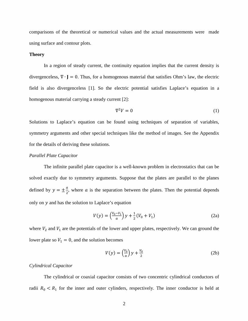
Parallel Plate Capacitor
The infinite parallel plate capacitor is a well-known problem in electrostatics that can be
solved exactly due to symmetry arguments. Suppose that the plates are parallel to the planes
defined by 𝑦 = ± 𝑎2, where 𝑎 is the separation between the plates. Then the potential depends
only on 𝑦 and has the solution to Laplace’s equation
𝑉(𝑦) = �𝑉0−𝑉1𝑎�𝑦 + 1
2(𝑉0 + 𝑉1) (2a)
where 𝑉2 and 𝑉1 are the potentials of the lower and upper plates, respectively. We can ground the
lower plate so 𝑉1 = 0, and the solution becomes
𝑉(𝑦) = �𝑉0𝑎� 𝑦 + 𝑉0
2 (2b)
Cylindrical Capacitor
The cylindrical or coaxial capacitor consists of two concentric cylindrical conductors of
radii 𝑅0 < 𝑅1 for the inner and outer cylinders, respectively. The inner conductor is held at
2

potential 𝑉0, and the outer conductor is held at potential 𝑉1. Due to the cylindrical symmetry, the
potential is independent of the azimuthal angle and depends only on the radial distance from the
central axis. The solution in all regions is given by
𝑉(𝑟) = �
𝑉0, 𝑟 < 𝑅0𝑉0 ln𝑅1−𝑉1 ln𝑅0
ln�𝑅1𝑅0�
+ 𝑉0−𝑉1ln�𝑅0𝑅1
�ln 𝑟 ,𝑅0 < 𝑟 < 𝑅1
𝑉1, 𝑟 > 𝑅1
(3a)
where 𝑟 = �𝑥2 + 𝑦2. If we ground the outer conductor so that 𝑉1 = 0, this simplifies to
𝑉(𝑥, 𝑦) =
⎩⎨
⎧𝑉0, 𝑟 < 𝑅0
𝑉0ln�𝑅0𝑅1
�ln ��𝑥
2+𝑦2
𝑅1� ,𝑅0 < 𝑟 < 𝑅1
0, 𝑟 > 𝑅1
(3b)
Line Charge Image
One way of finding the solution to Laplace’s equation for particularly convenient
geometries is to use the method of images, whereby image charges are placed outside of the
volume of interest such that the boundary conditions of the original problem are satisfied. Then
the potential inside the region of interest is uniquely defined and can be found using the charge
distribution of real and image charges. One such geometry consists of a line charge parallel to an
infinite grounded conducting plane, which has circular cylinder equipotential surfaces parallel to
the line charge. Thus, defining a circular equipotential in the homogenous material at a given
distance away from an infinite grounded plane is equivalent to placing an infinite line charge in
the material.
Suppose that the grounded plane is the 𝑦 = 0 plane (the 𝑥𝑧 plane), and that the circular
equipotential at voltage 𝑉0 is centered at (0, 𝑦0, 0) with radius 0 < 𝑅0 < 𝑦0. The potential
function that satisfies these boundary conditions and thus Laplace’s equation is
3

𝑉(𝑥, 𝑦) = 𝑉02asech�𝑅0𝑦0
�ln�
𝑥2+�𝑦+�𝑦02−𝑅02�2
𝑥2+�𝑦−�𝑦02−𝑅02�2� (4)
where 𝜀0 is the vacuum permittivity.
Parallel Plates with Insulator
Removing a portion of the conducting medium is equivalent to inserting an electrical
insulator in that region. Placing an insulator or a dielectric material in the conducting medium
has the effect of preventing current from flowing through the region of the dielectric. Thus,
current is forced to flow around the dielectric, and charges in the dielectric will tend to move
opposite of the external electric field, building up at the boundary of the dielectric. The result is
that there tends to be a higher potential near the positive electrode and a lower potential near the
negative electrode than if there were no dielectric present. In a homogenous, linear dielectric
material, the bound volumetric charge density is proportional to the free volumetric charge
density, so if no charge is embedded within the material, the material obeys Laplace’s equation
[2]. At the boundary, however, surface charges may still exist.
Apparatus and Methods
The electric potential field for each configuration was mapped using the PASCO
scientific MODEL PK-9023 Field Mapper set, which includes conductive paper, silver
conductive ink pen, a corkboard surface and metallic pins. The conductive ink was drawn onto
the paper and connected through the metallic pins to an Agilent E3610A power supply with a
fixed potential of 𝑉0 = 10.025 V. Since the ink has nonzero resistance, the pins were arranged in
a way that minimized the effects of the potential drop across the electrodes on the measurement
of the potential. These effects, however, should be small since the resistance of the paper is
roughly 5 to 6 orders of magnitude greater than the resistance of the ink. The electric potential
4

was then measured relative to the negative electrode with a Keithley Model 2000 DMM (input
resistance of at least 10 GΩ) at relevant points on the conductive paper. The electrode
configurations tested are shown in Figures 1 through 4.
6.00
14.00
Figure 1 Parallel plate capacitor configuration. The negative electrode is shown in thick black; the positive electrode is shown in thick red. The metallic pins on the electrodes are indicated by the small silver circles. Thick dotted lines indicate symmetry axes and the 𝑥𝑦 coordinate axes, while the intersections of thin dotted lines indicate measurement points and are separated by 1 cm in both dimensions. Using symmetry, only the upper left quadrant of the parallel plate capacitor was measured, from which the rest of the measurements can be inferred.
5

R 1.00
R 7.00
Figure 2 Cylindrical capacitor configuration. The negative electrode is shown in thick black; the positive electrode is shown in thick red. The metallic pins on the electrodes are indicated by the small silver circles. Thick dotted lines indicate symmetry axes and/or the 𝑥𝑦 coordinate axes, while the intersections of thin dotted lines indicate measurement points and are radially separated by 1 cm or in some cases 0.5 cm. Using symmetry, only the left half of the cylindrical capacitor was measured, from which the rest of the measurements can be inferred.
6

R 0.50
8.00
Figure 3 Line charge image configuration. The negative electrode is shown in thick black; the positive electrode is shown in thick red. The metallic pins on the electrodes are indicated by the small silver circles. Thick dotted lines indicate symmetry axes and the 𝑥𝑦 coordinate axes, while the intersections of thin dotted lines indicate measurement points and are separated by 1 cm in both dimensions.
7

12.0
0
4.00
6.00
12.00
Figure 4 Insulating box configuration. The negative electrode is shown in thick black; the positive electrode is shown in thick red. The metallic pins on the electrodes are indicated by the small silver circles. Thick dotted lines indicate symmetry axes and the 𝑥𝑦 coordinate axes, while the intersections of thin dotted lines indicate measurement points and are separated by 1 cm in both dimensions. The insulator—a cut out of the conducting paper—is placed symmetrically between the plates, as shown in grey.
Results and Analysis
Two-dimensional curve fits were performed in regions where the potential could be
analytically solved (ignoring edge effects) for each configuration. The fit parameters were then
compared to the actual values used for each configuration. The curve fits for the cylindrical
capacitor and parallel plate capacitor yielded parameter values that were close to the actual
values but were either not within their uncertainties, or the uncertainties were unreasonably
large. Of all configurations, the line charge configuration had the best agreement between the fit
parameters and the actual values. A qualitative and quantitative comparison can be made using
contour and surface plots that show the difference between measured values and theoretical
values of either analytical models or numerical solutions found by finite difference methods. The
8

measured and numerically calculated potential fields were linearly or cubically interpolated to
produce smoother surfaces for plotting.
Due to the high accuracy of the Kiethley 2000 DMM, voltage measurement uncertainties
were on the order of 0.1 mV, which corresponds to roughly 10−5 relative uncertainty in a typical
measurement. Thus, most of the uncertainty is in the theoretical model due to uncertainty in the
actual geometric parameters of the configurations. The uncertainty in each distance measurement
was typically 2 mm (about the width of the conductive ink), producing typical relative
uncertainties in the lengths of three percent or less. However, the uncertainties in the theoretical
voltage based on these parameters ranged from about 50 mV to 500 mV, and the relative
uncertainties ranged from one percent up to 70 percent. Typical relative uncertainties were
around 10 percent throughout most of the plane, though.
Parallel Plate Capacitor
The linear fit parameters in Eq. 2b for the region between the parallel plates were
𝑉0 = 9.4 ± 0.2 V and 𝑎 = 7.1 ± 0.2 cm, which are not within the uncertainty of the actual values
of 𝑉0 = 10.025 V and 𝑎 = 6.0 cm. Figures 5 and 6 show the surface and contour plots of the
measured potential with linear interpolation for the finite parallel plate capacitor.
9

Figure 5 Finite parallel plate capacitor potential field. The parallel plates are located at the sharp ridges, with the lower plate being groudned and the upper plate held at potential 𝑉0 = 10.025 V. The color (as well as the height) indicates the magnitude of the potential, with blue being small potential and red being large potential.
10
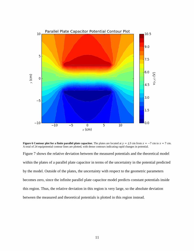
Figure 6 Contour plot for a finite parallel plate capacitor. The plates are located at 𝑦 = ±3 cm from 𝑥 = −7 cm to 𝑥 = 7 cm. A total of 24 equipotential contour lines are plotted, with dense contours indicating rapid changes in potential.
Figure 7 shows the relative deviation between the measured potentials and the theoretical model
within the plates of a parallel plate capacitor in terms of the uncertainty in the potential predicted
by the model. Outside of the plates, the uncertainty with respect to the geometric parameters
becomes zero, since the infinite parallel plate capacitor model predicts constant potentials inside
this region. Thus, the relative deviation in this region is very large, so the absolute deviation
between the measured and theoretical potentials is plotted in this region instead.
11
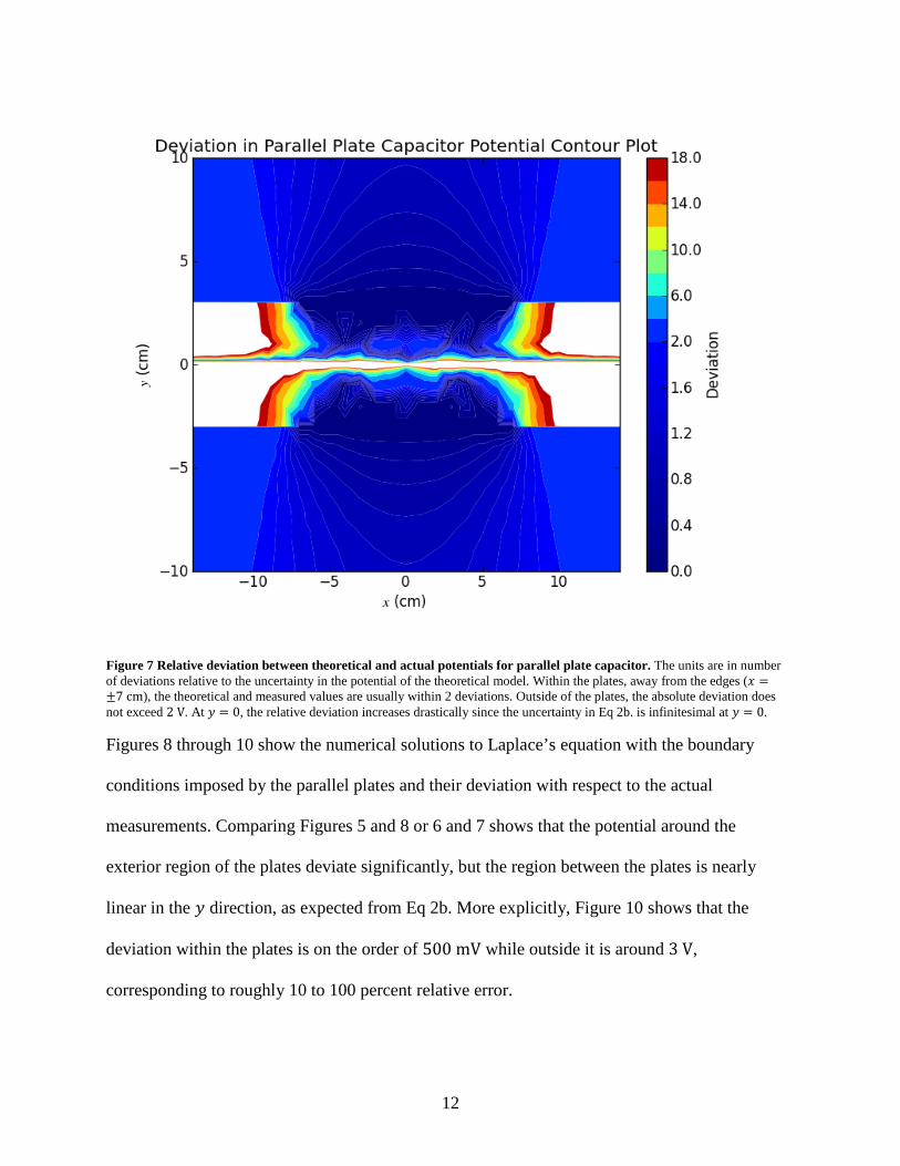
Figure 7 Relative deviation between theoretical and actual potentials for parallel plate capacitor. The units are in number of deviations relative to the uncertainty in the potential of the theoretical model. Within the plates, away from the edges (𝑥 =±7 cm), the theoretical and measured values are usually within 2 deviations. Outside of the plates, the absolute deviation does not exceed 2 V. At 𝑦 = 0, the relative deviation increases drastically since the uncertainty in Eq 2b. is infinitesimal at 𝑦 = 0.
Figures 8 through 10 show the numerical solutions to Laplace’s equation with the boundary
conditions imposed by the parallel plates and their deviation with respect to the actual
measurements. Comparing Figures 5 and 8 or 6 and 7 shows that the potential around the
exterior region of the plates deviate significantly, but the region between the plates is nearly
linear in the 𝑦 direction, as expected from Eq 2b. More explicitly, Figure 10 shows that the
deviation within the plates is on the order of 500 mV while outside it is around 3 V,
corresponding to roughly 10 to 100 percent relative error.
12

Figure 8 Surface plot of numerical solution to Laplace’s equation for the parallel plate capacitor. The solution area was initialized to a potential of 𝑉0
2 and the upper plate and lower plates were fixed at 𝑉0 = 10.025 V and 0 V, respectively.
13

Figure 9 Contour plot of numerical solution to Laplace’s equation for the parallel plate capacitor. The solution area was initialized to a potential of 𝑉0
2 and the upper plate and lower plates were fixed at 𝑉0 = 10.025 V and 0 V, respectively.
14

Figure 10 Absolute deviation between the numerical solution and measured potentials for the parallel plate capacitor.
Cylindrical Capacitor
In the region between the two cylinders, a curve fit to Eq. 3b produced parameters of
𝑉0 = 9.82 V, 𝑅0 = 1.03 cm and 𝑅1 = 6.98 ± 0.01 cm compared to the actual values of 𝑉0 =
10.025 V, 𝑅0 = 1.0 cm and 𝑅1 = 7.0 cm. The uncertainties in the voltage and inner radius fit
parameter were on the order of 1013 V and 105 cm, respectively, which are unrealistically large.
The outer radius is within two standard deviations of the actual value, and the voltage and outer
radius are both within three percent relative error. The contour and surface plots of the measured
potentials for the cylindrical capacitor configuration are shown in Figures 11 and 12.
15

Figure 11 Cylindrical capacitor surface plot. The inner cylinder at potential 𝑉0 = 10.025 V is located at the tip of the thorn-like peak, and the grounded outer cylder is located right at its base. The color (as well as the height) indicates the magnitude of the potential, with blue being small potential and red being large potential.
16

Figure 12 Contour plot for a cylindrical capacitor. The outer grounded conductor of radius 𝑅1 = 7 cm is near the dark blue ring, and the inner conductor of radius 𝑅0 = 1 cm is near the dark red ring. A total of 24 equipotential contour lines are plotted, with dense contours indicating rapid changes in potential.
The relative deviation between the theoretical potentials and actual potentials between the two
cylinders is shown in Figure 13. Outside of this region, Eq 3b model predicts constant potentials,
which corresponds to zero uncertainty with respect to the geometric parameters. Thus, in the
regions exterior to the cylindrical capacitor, the absolute deviation between the theoretical and
measured values is plotted (on the same scale).
17

Figure 13 Relative deviation between theoretical and actual potentials for cylindrical capacitor. The units are in number of deviations relative to the uncertainty in the potential of the theoretical model. Within the cylinders of radii 𝑅0 = 1 cm and 𝑅1 = 7 cm, the theoretical and measured potentials are nearly always within 2 deviations. Outside of this region, the cylindrical capacitor model predicts constant potentials, resulting in large relative deviations in these regions. The absolute deviations in these regions are typically less than 0.1 V.
The numerical solution to the cylindrical capacitor potentials is shown in Figures 14 and 15,
while the deviation compared to the measured potentials is shown in Figure 16. Examining
Figure 16, the largest deviations are near the peak; Figure 14 shows that there are jagged
outcrops in the peak, even after cubic interpolation. There is also a relatively large deviation
around the outer cylinder, which is probably due to the smoothing effect that the relaxation
method to solving Laplace’s equation has, causing the peak to be raised more around the base.
18
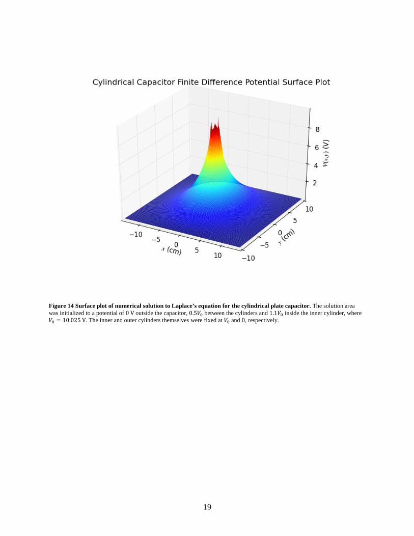
Figure 14 Surface plot of numerical solution to Laplace’s equation for the cylindrical plate capacitor. The solution area was initialized to a potential of 0 V outside the capacitor, 0.5𝑉0 between the cylinders and 1.1𝑉0 inside the inner cylinder, where 𝑉0 = 10.025 V. The inner and outer cylinders themselves were fixed at 𝑉0 and 0, respectively.
19

Figure 15 Contour plot of numerical solution to Laplace’s equation for the cylindrical capacitor. The solution area was initialized to a potential of 0 V outside the capacitor, 0.5𝑉0 between the cylinders and 1.1𝑉0 inside the inner cylinder, where 𝑉0 = 10.025 V. The inner and outer cylinders themselves were fixed at 𝑉0 and 0, respectively.
20

Figure 16 Absolute deviation between the numerical solution and measured potentials for the cylindrical plate capacitor.
Line Charge Image
The best fit parameters for Eq. 4 in the line charge image configuration were 𝑉0 =
11.8 V, 𝑦0 = 8.5 ± 0.1 cm and 𝑅0 = 0.53 cm compared to the actual values of 𝑉0 = 10.025 V,
𝑦0 = 8.0 cm and 𝑅0 = 0.5 cm. The relative uncertainty of the separation and radius are both
about six percent. Again the uncertainties in the voltage and radius were somewhat large at 15 V
and 2 cm, respectively, which would suggest (unreasonably) that the voltage and radius could
have been negative. Figures 17 and 18 show the potential surface and contour plots of the line
charge image configuration. Figure 19 shows the relative deviation for the line charge image.
21

Figure 17 Line charge image surface plot. A circular equipotential of radius 𝑅0 = 0.5 cm and potential 𝑉0 = 10.025 V is placed a distance 𝑦0 = 8.0 cm away from a grounded infinite conducting plane at 𝑦 = 0. The color (as well as the height) indicates the magnitude of the potential, with blue being small potential and red being large potential.
22

Figure 18 Line charge image contour plot. The 0.5 cm radius equipotential is centered at (0,8) cm and maintains constant potential of 𝑉0 = 10.025 V. The grounded conducting plane is at 𝑦 = 0. A total of 24 equipotential contour lines are plotted, with dense contours indicating rapid changes in potential.
23

Figure 19 Relative deviation between theoretical and actual potentials for line charge image. The units are in number of deviations relative to the uncertainty in the potential of the theoretical model. The relative deviation between the theoretical model and measured potentials is typically less than 2 deviations (i.e. below 𝑦 = 8 cm). Closer to the grounded plane (𝑦 = 0), the deviation is even less and falls within a single deviation.
Figures 20 and 21 show the numerical solutions to the line charge image configuration, and
Figure 22 shows its deviation from the measured potentials. The largest absolute deviations
occur near the peak around the equipotential, as shown by Figure 22.
24

Figure 20 Surface plot of numerical solution to Laplace’s equation for the line charge image. The solution area was initialized to a potential of 0.2𝑉0 everywhere except for the peak, which was initialized at 2𝑉0, where 𝑉0 = 10.025 V. Where the grid mesh intersected the circular equipotential, the potential was fixed at 𝑉0, and the plane along 𝑦 = 0 was fixed at 0.
25
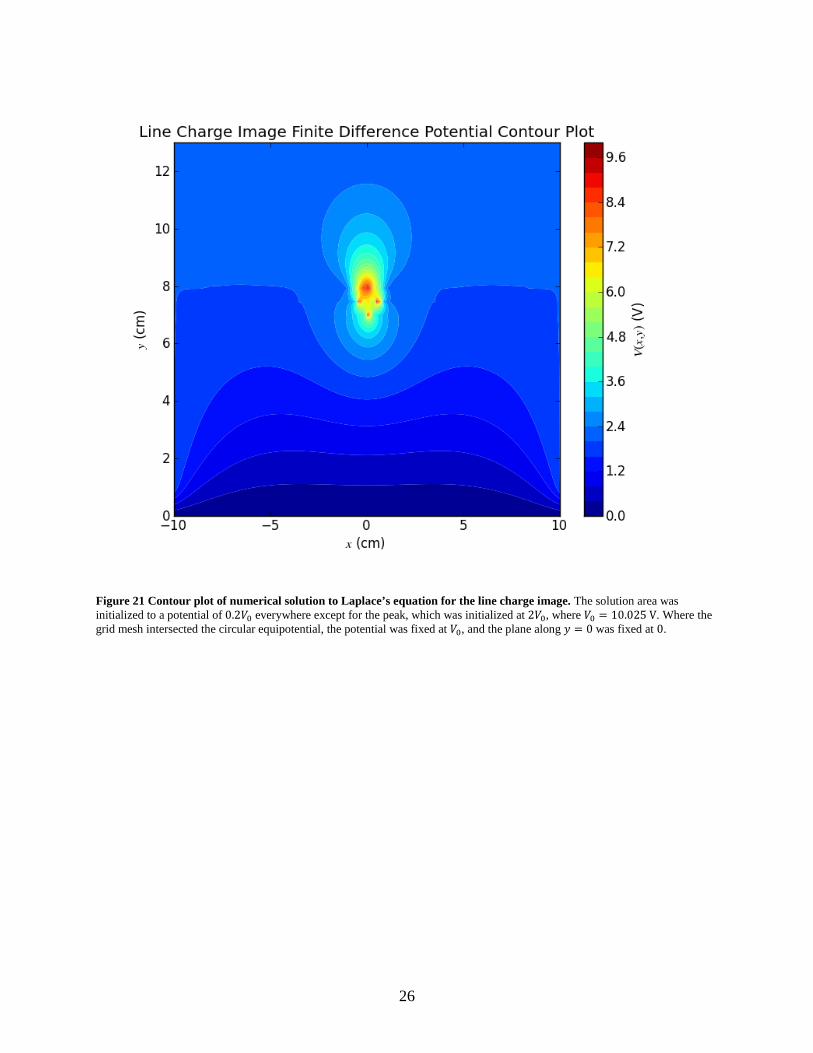
Figure 21 Contour plot of numerical solution to Laplace’s equation for the line charge image. The solution area was initialized to a potential of 0.2𝑉0 everywhere except for the peak, which was initialized at 2𝑉0, where 𝑉0 = 10.025 V. Where the grid mesh intersected the circular equipotential, the potential was fixed at 𝑉0, and the plane along 𝑦 = 0 was fixed at 0.
26

Figure 22 Absolute deviation between the numerical solution and measured potentials for the line charge image.
Parallel Plates with Insulator
Developing an analytic model or proper boundary conditions for a numerical solution
could not be achieved due to uncertainties in the boundary conditions and insufficient
information (such as the dielectric constant of the conductive medium). The potential within the
insulator was prohibitively difficult to measure, as it decrease almost monotonically or oscillated
around the grounded potential; only the potential at the boundary could be reliably determined.
Thus, Figures 23 and 24 show the surface and contour plots of the potential as measured in the
conductive medium and use grounded potential placeholder values in the insulator.
27

Figure 23 Insulating box surface plot. A box of dimensions 6 cm in the 𝑥 direction and 4 cm in the 𝑦 direction, centered at the origin, is depected with zero potential inside since only the boundary potential could be reliably determined. The positive and negative electrodes have potentials of 𝑉0 = 10.025 V and 0 V, respectively, and are located along the front and back edges (𝑦 = ±6 cm) with lengths of 12 cm. The color (as well as the height) indicates the magnitude of the potential, with blue being small potential and red being large potential.
28

Figure 24 Insulating box contour plot. The insulating box spans from −3 cm < 𝑥 < 3 cm and −2 cm < 𝑦 < 2 cm with grounded potential placeholder values inside. The electrodes are at 𝑦 = ±6 cm and have lengths of 12 cm. A total of 24 equipotential contour lines are plotted, with dense contours indicating rapid changes in potential.
Discussion and Conclusions
With the exception of the insulating box configuration, each of the configurations agreed
within one to two deviations of the theoretical model potential in regions where the model was
applicable. Qualitatively, the insulating box configuration behaved as expected, with smaller
potential drops between the dielectric and the electrodes. The parallel plate capacitor had
particularly large deviations on the edges and outside of the plates, where the theoretical model
of an infinite parallel plate capacitor was no longer valid. A model (see e.g. [3,4]) which
accounts for the strong electric fields on the edge of the plates would help to resolve this
29
discrepancy. The line charge image theoretical model also had very large deviations of 10 or
more times its uncertainty from the measured value around the original circular equipotential.
This is due to the theoretical model containing a pole that diverges logarithmically to infinity at
the point where the line charge would be located. In the laboratory, we would not expect to
measure such a diverging potential however, due to the finite dimensions of the experiment.
The numerical solutions to Laplace’s equation were not quantitatively in close agreement
with the measured values near sharp peaks and some of the boundaries, as can be seen in Figures
10, 16 and 22. Varying step sizes and initialization values have profound effects on the solution
results and convergence rates. For example, the parallel plate capacitor was initialized to a value
of 0.5𝑉0, which did not change for most of the grid throughout the iteration. Using a larger step
size would have propagated the boundary values more widely across the grid, resulting in a less
uniform potential outside the plates. Additionally, the larger step sizes tended to converge faster,
albeit with much less precision. Similarly, small step sizes would be better suited for computing
values near sharp peaks, such as those in the cylindrical capacitor and line charge image
configurations. However, computational memory limitations prevented smaller step sizes than
were used. Thus, either the algorithm must be further optimized, additional computational
resources obtained or the program rewritten in a more efficient computer language (e.g. C/C++).
Summary
The measured potentials agreed within one to two deviations of the theoretical model’s
potentials in most of the regions where the model was valid for each configuration.
Improvements to the analytic model that account for edge effects and the finite dimensions of the
geometry, although significantly more complicated, could decrease the deviation and increase
the extent of the agreement between the theoretical and measured potentials. The potential within
30

the insulator could not be reliably determined, and a theoretical comparison could not be made
due to insufficient information. However, the qualitative behavior of the potential around the
insulator was in agreement with expectations: regions around the insulator reduced the steady
currents and resulted smaller potential drops than if the insulator were absent. The numerical
solutions to Laplace’s equation agreed with the measured values in several regions of each
configuration, but the solution and convergence rate depended heavily on the initialization of the
method. Deviations of up to 100 percent were seen between the numerical solution and
measured potential, with larger deviations observed near areas of rapid potential change. Further
optimizations and experimentation with the initialization can be done to improve the relaxation
method results.
References
[1] Electric Fields Experiment Lab Manual. [2] D. J. Griffiths, Introduction to Electrodynamics, 3rd Ed. (Prentice Hall, New Jersey,
1999), p. 186, 288. [3] J. H. Jeans, The Mathematical Theory of Electricity and Magnetism, 2nd Ed. (Cambridge,
1911), p. 274-275. [4] W. Greiner, Classical Electrodynamics. (Springer, New York, 1998), p. 117-118.
Appendix: Solutions to Electrostatic Boundary Value Problems
Parallel Plate Capacitor
The infinite parallel plate capacitor with plates at 𝑦 = ± 𝑎2, where 𝑎 is the separation
between the plates permits a solution of the form 𝑉 = 𝑉(𝑦) by symmetry. Substituting this into
Laplace’s equation in Cartesian coordinates,
∇2𝑉 = 0 ⇒ �𝜕2
𝜕𝑥2+
𝜕2
𝜕𝑦2+𝜕2
𝜕𝑧2�𝑉(𝑦) = 0 ⇒
d2𝑉(𝑦)d𝑦2
= 0
which has a general solution 𝑉(𝑦) = 𝐴𝑦 + 𝐵. The boundary conditions require that
31

�𝑉 �−
𝑎2� = 𝑉1
𝑉 �𝑎2� = 𝑉0
⇒ �−𝐴𝑎2
+ 𝐵 = 𝑉2𝐴𝑎2
+ 𝐵 = 𝑉0⇒ �
𝐵 =12
(𝑉0 + 𝑉1)
𝐴 =𝑉0 − 𝑉1𝑎
where 𝑉1 and 𝑉0 are the potentials of the lower and upper plates, respectively. So the voltage
between the plates of an infinite parallel plate capacitor is given by Eq. 2a as
𝑉(𝑦) = �𝑉0 − 𝑉1𝑎
�𝑦 +12
(𝑉0 + 𝑉1)
Cylindrical Capacitor
The cylindrical capacitor consists of two concentric cylindrical conductors of radii
𝑅0 < 𝑅1 for the inner and outer cylinders, respectively. The inner conductor is held at potential
𝑉0, and the outer conductor is held at potential 𝑉1. Due to the cylindrical symmetry, the potential
is independent of the azimuthal angle and depends only on the radial distance from the central
axis: 𝑉 = 𝑉(𝑟). Substituting this into Laplace’s equation in cylindrical coordinates,
∇2𝑉 = 0 ⇒ �1𝑟𝜕𝜕𝑟�𝑟
𝜕𝜕𝑟� +
1𝑟2
𝜕2
𝜕𝜙2 +𝜕2
𝜕𝑧2�𝑉(𝑟) = 0 ⇒
1𝑟
dd𝑟�𝑟
d𝑉(𝑟)d𝑟
� = 0
The general solution is 𝑉(𝑟) = 𝐴 + 𝐵 ln 𝑟. In the region for 𝑟 < 𝑅0, the boundary conditions
require that the potential be finite everywhere, so
�|𝑉(0)| ≠ ∞𝑉(𝑅0) = 𝑉0
⇒ �𝐵 = 0𝐴 = 𝑉0
In the region for 𝑅0 < 𝑟 < 𝑅1, the boundary conditions are
�𝑉(𝑅0) = 𝑉0
𝑉(𝑅1) = 𝑉1⇒ �𝐴 + 𝐵 ln𝑅0 = 𝑉0
𝐴 + 𝐵 ln𝑅1 = 𝑉1⇒
⎩⎪⎨
⎪⎧𝐴 =
𝑉0 ln𝑅1 − 𝑉1 ln𝑅0
ln �𝑅1𝑅0�
𝐵 =𝑉0 − 𝑉1
ln �𝑅0𝑅1�
In the region for 𝑟 > 𝑅1, we again require that the potential be finite everywhere, so
32

�|𝑉(∞)| ≠ ∞𝑉(𝑅1) = 𝑉1
⇒ �𝐵 = 0𝐴 = 𝑉1
Then the complete solution is
𝑉(𝑟) = �
𝑉0, 𝑟 < 𝑅0𝑉0 ln𝑅1−𝑉1 ln𝑅0
ln�𝑅1𝑅0�
+ 𝑉0−𝑉1ln�𝑅0𝑅1
�ln 𝑟 ,𝑅0 < 𝑟 < 𝑅1
𝑉1, 𝑟 > 𝑅1
where 𝑟 = �𝑥2 + 𝑦2.
Line Charge Image
The potential for the configuration with a single line charge running parallel to an
infinite, grounded conducting plane can be solved using the method of images by placing an
image line charge of opposite charge density an equal distance away on the other side of the
plane. Suppose that a line charge of charge density 𝜆 is a distance 𝑦 = 𝑎 away from the
conducting plane defined by 𝑦 = 0 (i.e. the 𝑥𝑧 plane) and that the line charge runs parallel to the
𝑧 axis at 𝑥 = 0. Then an image line charge of charge density – 𝜆 is placed at 𝑦 = −𝑎 parallel to
the 𝑧 axis at 𝑥 = 0 as well. From cylindrical symmetry, Gauss’s law can be used to calculate the
electric field around a line charge:
�𝐄 ∙ d𝐀𝑆
=𝑄𝜀0⇒ 𝐸(𝑟)�𝐫� ∙ d𝐀
𝑆=
1𝜀0�𝜆(𝑙′)d𝑙′𝐶
⇒ 𝐸(𝑟)�d𝐴𝑆
=1𝜀0𝜆𝐿 ⇒ 𝐸(𝑟)(2𝜋𝑟𝐿) =
1𝜀0𝜆𝐿
⇒ 𝐸(𝑟) =1
2𝜋𝜀0𝜆𝑟⇒ 𝐄(𝐫) = 𝐸(𝑟,𝜙, 𝑧) =
12𝜋𝜀0
𝜆𝑟𝐫�
where 𝐫� points out from the line charge.
Then the potential is defined by 𝑉(𝐫) = −∫ 𝐄 ∙ d𝐥𝐫𝒪 where 𝒪 = (0,0,0), which
corresponds to a radial displacement 𝑟 = 𝑎 in cylindrical coordinates from the line charge. Thus,
𝑉(𝐫) = −� 𝐄(𝐥′) ∙ d𝐥′𝐫
𝒪= −�
12𝜋𝜀0
𝜆𝑟′𝐫� ∙ d𝑟′𝐫�
𝑟
𝑎= −
𝜆2𝜋𝜀0
[ln|𝑟′|]𝑎𝑟 =𝜆
2𝜋𝜀0ln �
𝑎𝑟�
33

The radial distance from the line charges is given by 𝑟± = �𝐫 − 𝐫±� = �𝑥2 + (𝑦 ∓ 𝑎)2, and we
use superposition to write the potential due to each line charge:
𝑉(𝐫) = 𝑉(𝑥,𝑦, 𝑧) = 𝑉−(𝐫) + 𝑉+(𝐫) =−𝜆
2𝜋𝜀0ln �
𝑎𝑟−� +
𝜆2𝜋𝜀0
ln �𝑎𝑟+� =
𝜆2𝜋𝜀0
ln �𝑟−𝑟+�
=𝜆
2𝜋𝜀0ln�
�𝑥2 + (𝑦 + 𝑎)2
�𝑥2 + (𝑦 − 𝑎)2� =
𝜆4𝜋𝜀0
ln�𝑥2 + (𝑦 + 𝑎)2
𝑥2 + (𝑦 − 𝑎)2�
The equipotential surfaces can then be found by setting 𝑉(𝐫) = 𝑉0, where 𝑉0 is the potential of
that surface. The result is a function of 𝑥 and 𝑦 in terms of the parameters 𝑎, 𝜆 and 𝑉0 that
defines equipotential surfaces that are circular cylinders centered at �0,𝑎 coth �2𝜋𝜀0𝑉0𝜆
� , 𝑧� for all
𝑧 ∈ ℝ and of radius 𝑅 = 𝑎 �csch �2𝜋𝜀0𝑉0𝜆
��.
Then defining a circular equipotential surface at voltage 𝑉0 and of radius 𝑅0 =
𝑎 �csch �2𝜋𝜀0𝑉0𝜆
�� in the material at a distance 𝑦0 = 𝑎 coth �2𝜋𝜀0𝑉0𝜆
� away from the plane defines
the corresponding line charge location 𝑦 = 𝑎 and charge density 𝜆. This permits the solution
given above for the voltage in the region of interest. To find 𝑎 and 𝜆,
�𝑦0 = 𝑎 coth �
2𝜋𝜀0𝑉0𝜆
�
𝑅0 = 𝑎 �csch �2𝜋𝜀0𝑉0𝜆
��⇒
⎩⎪⎨
⎪⎧𝑎 = �𝑦02 − 𝑅02
𝜆 =2𝜋𝜀0𝑉0
asech �𝑅0𝑦0�
These solutions are valid provided that 0 < 𝑅0 < 𝑦0. Thus, the potential in the region of interest
is
𝑉(𝐫) = 𝑉(𝑥, 𝑦) =𝑉0
2 asech �𝑅0𝑦0�
ln�𝑥2 + �𝑦 + �𝑦02 − 𝑅02�
2
𝑥2 + �𝑦 − �𝑦02 − 𝑅02�2�
34