measurement of evapotranspiration with … of evapotranspiration with ... c3 to c4 plants and...
TRANSCRIPT

MEASUREMENT OF EVAPOTRANSPIRATION WITH
COMBINED REFLECTIVE AND THERMAL INFRARED
RADIANCE OBSERVATIONS
Final Report Submitted To:
The National Aeronautics
And Space Administration,
Washington, D.C.
Grant No. NAG 5-911
1/87 8/93
Allen S. Hope
Principal Investigator
Department of Geography
San Diego State University
San Diego, CA 92182
1993
https://ntrs.nasa.gov/search.jsp?R=19940016478 2018-06-03T13:34:19+00:00Z


ACKNOWLEDGEMENTS
The research summarized in this report was based on data collected at the
FIFE study site in 1987 and 1989 by a large number of investigators from
other institutions, along with their technical staff and graduate students.
This generous contribution and the considerable assistance given by the
staff of the FIFE Information System (FIS) under the leadership of Dr.
Donald Strebel, is gratefully acknowledged. I am indebted to Dr. Forrest
Hall and Dr. Piers Sellers for the support, scientific guidance and
inspiration they provided throughout the project.
This study was part of a collaborative research effort with Dr.
Samual Goward at the University of Maryland. The regular meetings and
discussions with Dr. Goward significantly influenced many of the ideas
and investigations summarized in this report. I very much appreciate
Dr. Goward's significant contribution to my scientific development over
the past decade.
The results summarized in this report have been drawn from a number
of published and unpublished studies conducted in collaboration with co-
investigators or graduate students. The contributions made by the
following collaborators is acknowledged (primary chapters in parentheses):
Andrew Abouna (6) Eugene Peck (Appendix 1)
Tom McDowell (2, 3, 4) Sally Westmoreland (Appendix 2)
Frederick Mertz (Appendix 2) Douglas Stow (Appendix 2)


TABLE OF CONTENTS
1. INTRODUCTION ................................................................................... 1
1.3
Background ................................................................................... 1
Hypothesized Relationship BetweenLE, Ts and SVl .................................................................................... 2
Objectives and Approach ............................................................. 3
2. THE TS-NDVl RELATIONSHIP: SENSOR SYSTEMS
AND ATMOSPHERIC EFFECTS ................................................................... 6
2.1
2.2
2.3
Background ................................................................................... 6
Data Sources and Processing ..................................................... 6
Atmospheric Corrections of ReflectedRadiances ................................................................................... 8
Results and Discussion ................................................................. 10
Conclusion ................................................................................... 14
3. FACTORS AFFECTING THE TS-NDVl RELATIONSHIP:
LOCAL SCALE ................................................................................... 16
3.1 Introduction ................................................................................... 16
3.2 Window Size ................................................................................... 17
3.3 Ts-NDVl Regression Slope Soil Moisture and LE ............ 18
3.3.1
3.3.2
3.3.3
3.3.4
3.3.5
Specific objectives .......................................................... 18
Methodology ......................................................................... 21
Analytical procedures ..................................................... 22Results and discussion ................................................... 22
Conclusion ............................................................................ 35
3.4 Burn Treatments and Other Landscape Controls ................ 36
3.4.1
3.4.2
3.4.3
3.4.4
3.4.5
Background ........................................................................... 36Specific objectives ......................................................... 39
Methodology ......................................................................... 40Results and discussion .................................................. 44
Conclusions ......................................................................... 49

3.5 Regression Residuals .....................................................................50
3.5.1 Spatial pattern of Ts residuals ..................................513.5.2 Relationship between Ts residuals and
solar radiation ...................................................................53
4. REGIONAL ANALYSES OF THE TS-NDVIRELATIONSHIP ...................................................................................5 5
4.1 Introduction ....................................................................................554.2 Ts-NDVI Relationship for Different
Land-Cover Types ............................................................................554.3 Analysis of Ts-NDVI Time Series ............................................59
4.3.14.3.24.3.34.3.4
Objective ..............................................................................59AVHRR data processing ..................................................59Results and discussion ...................................................63Conclusions .........................................................................68
5. LOCAL SCALE MODELING OF LE FLUXESAND TS................................69
5.1 Introduction ....................................................................................695.2 The Original Tergra Model and Applications .......................705.3 A Modified Tergra Model ...............................................................73
5.3.15.3.25.3.35.3.45.3.55.3.6
Background ..........................................................................73The modified Tergra model (Tergra-2) .................... 73Experimental goals and methodology ......................78Results ..................................................................................84Discussion ............................................................................91Conclusions .........................................................................95
6. MODELING LARGE AREA LE FLUXESAND TS ........................................9 7
6.16.26.3
Background ...........................................................................97Study Objectives ..............................................................97Methodology ........................................................................99
ii

°
6.4
CONCLUSIONS
REFERENCES
APPENDICES
Appendix 1
Appendix 2Appendix 3
6.3.1 Research data ..................................................... 100
6.3.2 Modeling area averaged LE and Ts .............. 102
6.3.3 Modeling spatial patterns of
LE and Ts ................................................................ 105
Conclusions ......................................................................... 108
................................................................................... 09
................................................................................... 12
................................................................................... 124
Peck and Hope (1993) ...................................... A 1
Mertz et al. (1993) ............................................ A2Research Publications ..................................... A3
iii

LIST OF TABLES
2.1
2.2
2.3
3.1
3.2
3.3
3.4
3.5
3.6
5.1
5.2
5.3
5.4
Flux station characteristics and NS001 view anglefor June 6, 1987 ........................................................................................ 8
NDVI and surface temperature means and coefficientsof variation for observations made by three sensors ......................... 13
Scheffe F-test scores for comparison of Ts-NDVI
regression slopes ..................................................................................... 14
Significance of Scheffe F-scores for Ts-NDVI
regression slope differences using three window sizes ................... 19
Volumetric soil moisture content (%) at 25 mm depthat four test sites on three dates .............................................................. 21
Slope, intercept, standard error (SE) and coefficient
of determination (r2) for the regression of Ts on NDVIfor each station ......................................................................................... 23
Sites with Ts-NDVI regression slopes that were notsignificantly different from each other .................................................. 25
Percentage of each sub-scene categorized as burntgrass, agricultural land, forest, steep slopes (> 6%),moderate slopes (3-6%), hill tops and valley bottoms ...................... 41
Coefficient of determination for the regression of the
mean NDVI (NDVI), mean Ts (Ts) and SL on the percent
of total burnt grassland (B.TOTAL), burnt grassland on hilltops (B.T), moderate slopes (B.M), steep slopes (B.ST),steep north facing slopes (B.ST.N), steep south facing slopes(B.ST.S) and steep east and west facing slopes (B.ST.EW) ........... 45
Characteristics of the four experimental flux measurementstations in 1987 ........................................................................................ 79
Characteristics of the four experimental flux measurementstations in 1989 ........................................................................................ 79
Simulation periods, NDVI, mean canopy height, ratio ofC3 to C4 plants and initial soil water potential at 10 cmdepth for each station .............................................................................. 80
Root-mean-square errors are given in watts per squaremeter .......................................................................................................... 84
iv

6.3
Tergra-2 GIS parameters for the four major soil series .................... 101
Comparison at three times on June 6, 1987 of observedLE (Obs) and estimated LE using Tergra-2 GIS andAVHRR NDVI, TM Kauth-Thomas GN (GN1) and theaverage Kauth-Thomas GN (GN2) for each cell ................................ 103
Mean and coefficient of variation for observed Ts and
estimated Ts using Tergra-2 GIS and AVHRR NDVI,
TM Kauth-Thomas GN (GN1) and the averageKauth-Thomas GN (GN2) for each cell ................................................ 104
V

1.1
2.1
2.2
3.1
3.6
3.7
3.10
4.1
4.2
4.3
LIST OF FIGURES
Proposed relationship between remotely sensedspectral vegetation indices and surface temperature ....................... 2
Surface temperature versus NDVI scatterplots forMMR, NS001 and AVHRR observations ............................................. 11
Surface temperature versus NDVI scatterplots forMMR, NS001 and AVHRR observations ............................................. 12
Examples of the Ts-NDVI scatterplots from stations2, 8 and 36 ................................................................................................ 24
Linear least squares regression lines for 17 subscenes .................. 26
Relationship between Ts-NDVI regression slopes andLE-G ........................................................................................................... 30
Relationship between Ts and the NDVI for station 36 ...................... 32
Relationship between Ts-NDVI regression slope andsoil moisture ............................................................................................. 34
Scatterplot of Ts versus NDVI for burnt and unburnt areas
of the Konza prairie ................................................................................. 38
Dendrogram illustrating clustering of flux station on thebasis of slope-cover-treatment .............................................................. 42
Hierarchy of burn-terrain independent variables .............................. 43
Scatterplots of the Ts-NDVI regression slope (SL)versus the area of each sub-scene ...................................................... 46
Image of residuals from the regression of Ts on NDVIfor station 8 ............................................................................................... 52
Scatterplots of Ts versus NDVI using AVHRR data for
selected land-cover types in Kansas ................................................... 57
AVHRR mean Ts and NDVI for different land-cover typesover Kansas .............................................................................................. 58
Visually assessed percentage cloud cover in AVHRRobservations ............................................................................................. 63
vi

4.4
4.5
5.1
5.2
5.3
5.4
5.5
5.6
5.7
5.8
6.1
6.2
6.3
6.4
Observed relation between the Ts and NDVI on 12selected dates in 1987...........................................................................65
Slope and intercept of Ts-NDVI relationship compared tosensor view zenith angle ......................................................................66
Arrangement of soil, plant and atmospheric resistancesin the Tergra model.................................................................................72
Difference between simulated grass canopy temperatureon a horizontal surface and simulated values on fourslope-aspect combinations....................................................................72
Relationship between the derivative of g c with respect toKpar and the NDVI calculated using MMR data collectedfrom a helicopter......................................................................................81
Observed LE and Tergra-2 estimated LE for the periodJune 4-6, 1987.........................................................................................85
Observed LE and Tergra-2 estimated LE for the periodAugust 15-17, 1987.................................................................................86
Observed LE and Tergra-2 estimated LE for the periodAugust 3-4, 1989......................................................................................87
Observed LE and Tergra-1 estimated LE for sites 908 and944 for the August 1989 simulation period......................................... 89
Observed canopy temperature using a helicopter-mountedMMR versus Tergra-2 estimates of canopy temperature.................. 95
Comparison of observed and modeled LE using the AVHRRNDVI, TM Kauth-Thomas GN and the averageKauth-Thomas GN...................................................................................103
Observed and estimated LE at 10 flux measurement stationson June 4, 1987.......................................................................................105
Observed versus estimated LE at the flux measurementstations on June 4, 1987........................................................................106
AVHRR derived surface temperature (June 6, 1987)versus surface temperature modeled using three differentspectral vegetation index approaches in Tergra-2 GIS................... 107
vii

1. INTRODUCTION
1.1
A negative and linear relationship between surface temperature (Ts)
and a spectral vegetation index (SVI) has been observed using data
collected over a variety of landscape types and with different sensors
(Gurney et al. 1983; Goward et al. 1985; Hope et al. 1986; Whitehead et al.
1986; Goward and Hope 1989; Nemani and Running 1989; Carlson et al.
1990; Price 1990; Hope 1992). Changes in the characteristics of the
relationship between Ts and a SVI (e.g., slope of the regression line) were
hypothesized to be indicative of variations in latent heat flux (LE) (Hope,
Petzold et al. 1986). The possibility of using the Ts-SVI relationship to
predict LE was investigated as part of the First International Satellite
Land Surface Climatology Project (ISLSCP) Field Experiment (FIFE).
Results from this project are summarized in the following chapters.
A theoretical basis for the Ts-SVI investigation was provided by
Hope (1986) who used an integrated energy balance-spectral reflectance
model to demonstrate that variations in soil moisture, and hence LE
fluxes, may affect the slope of the linear least squares regression of Ts on
the normalized difference vegetation index (NDVI). Goward and Hope
(1986) extended this concept in designing a research strategy to
investigate whether the characteristics of the Ts-NDVI regression were
indicative of variations in LE over the FIFE study site (Konza prairie).

1.2 Hvoothesized Relationshio Between LE. Ts and SVI
The hypothesized relationship between LE, Ts and a SVI was
presented by Goward and Hope (1986) and Goward and Hope (1989) and is
illustrated in Figure 1.1.
SOIL MIN.LE
TS
SOIL MAX.
LE
LE
NOLE
MAX. LE
BARE FULL
SOIL NDVI CANOPY
Figure 1.1" Proposed relationship between remotely sensed spectral
vegetation indices and surface temperature. Hypothesized
lines of equal LE flux are indicated (Goward and Hope 1986).
Remotely sensed surface temperatures will vary as a function of
vegetation canopy cover, even in the absence of LE because the thermal
inertia of the vegetated interface is lower than that of the substrate.
Transpiring vegetation further reduces Ts because of the energy used for
LE. Vegetation also reduces ground heat flux (G) and, as Kustas (1989) has
shown, SVIs can be used to predict G. A fundamental assumption in Figure
1 is that the SVI is an indicator of fractional vegetation cover, an
assumption substantiated by Huete et al. (1985). The area averaged LE

illustrated in Figure 1.1 were thus considered to be related to the SVl and
Ts by way of the relative contributions of evaporation from bare soil and
vegetation under different soil moisture conditions. Since Ts is also
affected by meteorological conditions and differences in surface
roughness, variations in these conditions can also affect the nature of the
Ts-SVl relationship. A more realistic representation of the relationships
given in Figure 1.1 may thus include surface temperatures "normalized"
for these variations.
1.3 Objectives and Aooroach
The broad goal of the research summarized in this report was "To
facilitate the evaluation of regional evapotranspiration (ET) through the
combined use of solar reflective and thermal infrared radiance
observations" (Goward and Hope 1986, p. 5). The specific objectives
stated by Goward and Hope (1986) were to:
1) Investigate the nature of the relationship between Ts and the NDVI and
develop an understanding of this relationship in terms of energy exchange
processes, particularly LE.
2) Develop procedures to estimate large area LE using combined Ts and
NDVI observations obtained from AVHRR data.
3) Determine whether measurements derived from satellite observations
relate directly to measurements made at the surface or from aircraft
platforms.
Both empirical and modeling studies were used to develop an
understanding of the Ts-NDVI relationship. Most of the modeling was
based on the Tergra model (Soer 1977) as originally proposed by Goward

(1986). This model, and modified versions developed in this project,
simulates the flows of water and energy in the soil-plant-atmosphere
system using meteorological, soil and vegetation inputs. Model outputs
are the diurnal course of soil moisture, Ts, LE and the other individual
components of the surface energy balance. This model was originally
selected for the study since:
1) The model was developed specifically for application to grassland
situations and was thus considered to be suitable for the Konza prairie.
2) Tergra had been tested previously by numerous investigators and had
generally been shown to be an accurate simulator of LE and Ts (Huygen and
Reiniger 1977; Soer 1980; Hope, Petzold et al. 1986).
3) The simple model structure can be readily modified and the data needs
are not excessive.
4) Tergra had been interfaced with a canopy reflectance model (SAIL) by
Hope (1988) which provided for the combined simulation of Ts and the
NDVI if necessary.
The general sequence of research activities followed in this project
was to:
1) Conduct a series of empirical studies to determine how the Ts-NDVI
relationship changes with different sensors/platforms, variations in land
cover/use and treatment, terrain, soil moisture and surface energy
balance. This component of the study examined the relationship at local
and regional scales.
2) Use the Tergra model and modified versions of this model to integrate
SVI and Ts observations into the modeling of LE at point locations within
the FIFE study area.
4

3) Model spatial patterns of LE using data from the AVHHR system (Ts and
the NDVI) and the modified Tergra model developed in 2).
The study was regarded as part of the integrative science activities
of FIFE and so every attempt was made to incorporate findings from other
FIFE investigations. Also, the project utilized data from a wide range of
remote sensing systems (non-imaging radiometers held by hand or
mounted on a helicopter, the NS001 data collected by the C-130 aircraft,
Thematic Mapper (TM) and NOAA 9 and 10 satellite data (AVHRR)). As the
project evolved, the need for information on the spatial patterns of soil
moisture became apparent and the scope of the project was increased to
include a component of soil moisture mapping in collaboration with E.
Peck of the Hydex Corporation (Vienna, VA). This research is described in
Appendix 1. Collaborative research with Photon Engineering (San Diego,
CA) was also initiated later in the project with the goal of implementing
and testing an easy to use, state-of-the-art atmospheric correction
routine. This collaboration was under the direction of F. Mertz and the
research is described in Appendix 2.
5
2. THE Ts-NDVI RELATIONSHIP: SENSOR SYSTEMS
AND ATMOSPHERIC EFFECTS
2.1 I_TJ_szmld.
Data collected during the FIFE were valuable for determining how
the Ts-NDVI relationship varied because of differences in data collection
systems (differences in spectral and spatial resolution) and atmospheric
conditions. These variations needed to be understood and quantified if the
relationship was to be used to predict LE. An initial study was designed
to investigate how sensor/platform and atmospheric conditions could
affect the Ts-NDVI relationship. The relationship was compared using
data collected with a Barnes modular multiband radiometer (MMR), NS001
Thematic Mapper simulator and NOAA Advanced Very High Resolution
Radiometer (AVHRR). These data were all collected on a single date,
June 6, 1987.
2.2 Data Sources and Processing
The MMR data were collected using the NASA H-1 (Huey) helicopter
flown at 230 m agl. The 1_ field-of-view of the MMR had a ground
resolution of approximately 4 m. The data were collected between 1141
and 1251 CDT or 1609 and 1643 CDT. Approximately 30 observations were
made over each flux measurement station (within a 5 minute period).
Reflectances were calculated by ratioing the observed reflected spectral
radiances to radiances collected over a calibration sheet (details are
contained in the FIFE Information System - FIS). Arithmetic means from
6
the 30 observations were used to determine the NDVI and Ts at each flux
station.
The NS001 instrument was mounted on a NASA C-130 aircraft flown
at approximately 4,800 m agl, giving a ground resolution of approximately
12 m at nadir. Only data from flight lines parallel to the solar plane were
used in the study. An 80 x 80 box of pixels around each flux station was
extracted from the NS001 imagery. Two adjacent flight lines covered all
of the flux stations used in this study and the maximum view (scan) angle
for any station was 30oo. Seventeen flux stations were located using the
latitude-longitude geocoding provided by the FIS. Sub-images were
rectified to be oriented north-south. The NS001 thermal counts were
converted to apparent surface temperatures using the procedure and
constants provided by the FIS. This technique does not account for
atmospheric attenuation of thermal radiances. The station
characteristics and NS001 view angle for each station are given in
Table 2.1.
The AVHRR image was acquired by the NOAA 9 Polar Orbiter satellite
at 1636 CDT over the FIFE site on June 6, 1987. The view angle was 34.9 °
which resulted in a ground resolution of 1.34 km. Pixels corresponding to
the FIFE site were extracted from the full scene after geometric
rectification. Apparent Ts was calculated for both AVHRR thermal bands
using the equations provided in the NOAA Polar Orbiter User's Guide
(Kidwell 1986). These two temperatures were then used to obtain a
"corrected" Ts using the split window technique described by Price (1984).
Emissivity over the FIFE study site was taken to be 1.0.
7

Table 2.1: Flux station characteristics and NS001 view angle forJune 6, 1987.
Station Oharacteristics*
02 UB
06 LM
O8 BM
1 0 BB12 US
14 LM1 8 BT
20 BM22 BM
24 LM
28 BM
34 BM
36 LM
38 LM
40 BS
42 BS44 BT
View Angle !Deg.)8.4
1.1
22.0
23.9
15.4
11.4
257
146
29 9
217
30 0
254184
184224
173
O3
The first letter represents unburned (U) or burned (B)
and the second letter represents valley bottom (B),
moderate slope (M), steep slope (S) or plateau top (T).
2.3 Atm0,$pherio Corrections of Reflected Radiances
Red and near infrared MMR reflectances (obtained using a reference
target calibration procedure) provided by the FIS were taken to be
standard ("correct") values. The NS001 and AVHRR data were, however,
not corrected for atmospheric scattering of the reflected radiation. The
improved dark object subtraction technique (Chavez 1988) was selected
as a means for removing the effects of atmospheric scattering from the
8

NS001 and AVHRR red and near infrared observations.
The dark object subtraction technique is based on the assumption
that completely shadowed pixels should have radiances close to zero in
the visible bandwidths, with values above zero being attributed to
contributions from atmospheric scattering. Traditional dark object
subtraction techniques require an examination of the histogram of each
band to determine the "take-off point", or the point of separation between
shadowed and illuminated pixels (Chavez 1988). This radiance value
becomes a "haze correction" value for the band and is then subtracted from
the radiance values for all pixels. The improved technique incorporates
two factors: the wavelength dependency of atmospheric scattering and the
relative radiometric sensitivities of the sensor's channels (Chavez 1988).
The improved technique requires the user to assess the overall
atmospheric conditions at the time of the scene acquisition, selecting
from: very clear, clear, moderate, hazy and very hazy. The amount of
atmospheric scattering in each of the sensors channels varies depending
on the designation of atmospheric condition (clear - approaches Rayleigh
scattering; very hazy - approaches Mie scattering). Based on this
wavelength dependency, Chavez (1988) developed a set of equations for
calculating the amount of scattering for the visible and near infrared
bands of a sensor. Equations are specific to the designated atmospheric
condition.
The next step in the improved technique requires histogram analysis
of one of the visible channels to determine the haze correction value for
the selected band. Haze corrections in the other bands are then calculated
using the scattering model appropriate to the general atmospheric
conditions. The calculated haze values are adjusted ("normalized") for the
9

gains and offsets of each band. Thus, the haze values are scaled to the
appropriate digital number (DN) range for each band. Finally, the
normalized haze values are subtracted from the brightness values for all
pixels.
The darkest object subtraction technique is unsuited to AVHRR data
because the large pixels almost certainly preclude the possibility of
obtaining completely dark/shadowed areas in the instantaneous field-of-
view (IFOV). However, the technique was applied to these data to make a
"relative" correction for the effects of atmospheric scattering. The red
band was used for the histogram analysis step for the AVHRR data (the
only visible band) while the blue band was selected for the analysis of the
NS001 data since it had the most distinct division between apparently
shaded and unshaded pixels in the histogram.
2.4 Results and Discussion
Helicopter MMR data were available for nine flux stations on June 6,
1987 and were used to determine station Ts and NDVI reference values
(assumed to be true). NS001 data were analyzed for the same nine
stations by first extracting a window of 80 x 80 pixels centered on the
station and then calculating the mean Ts and NDVI values for each station.
Since it is not possible to precisely locate AVHRR pixels over each flux
station, 16 random pixels were selected for the comparison with MMR and
NS001 observations. The scatter plots of Ts versus the NDVI for each
sensor with no correction for atmospheric scattering is given in
Figure 2.1.
I 0

0 0
308.0 -
307.0
_306.0
I,in,- 305.0
',' 304.0n=tILl
303.0ILl¢_)
302.0n-
(/3
301.0
300.0
m
299.00.30
#
+++
xx
X
_kx
)o¢x
o
o
0
o
o
0
0
0 - MMR DATA
X- NSO01 DATA
+ - AVHRR DATA
i i i i i i i i _ I I i i i I i i i I i I I I i I I i i , I
0.40 0.50 0.60 0.70 0.80 0.90NDVI
Figure 2.1 Surface temperature versus NDVI scatterplots for MMR,NSO01 and AVHRR observations - no haze corrections.
While the negative and linear relationship between Ts and the NDVi
was observed using data collected by the three different sensors, it is
apparent from Figure 2.1 that:
1) The MMR data exhibited the largest range in Ts values.
2) NDVl values decreased with height of the sensor above the Earth's
surface.
When the haze corrections are applied to the red and near infrared data,
II

the NSO01 and AVHRR scatter plots align with the MMR points (Figure 2.2).
This is verified by the summary statistics given in Table 2.2 where the
range in mean NDVIs for the three sensors is reduced substantially after
the correction is applied.
0 0
3b8.o -
307.0
,_, 306.0V
r,,..305.0
_ 304.0
N 303.0wC.)
_ 302.0
301.0
300.0
I
==
299.00.30
#0
++ o+0
0
_+
Ox
O
x xx
0 - MMR DATA
X - NSO01 DATA
+ - AVHRR DATA
i i i i I ' i i i I i i i i I a i i i I I i i i I i i i w I0.4-0 0.50 0.60 0.70 0.80 0.90
NDVI
Figure 2.2: Surface temperature versus NDVI scatterplots for MMR,NSO01 and AVHRR observations - haze corrected.
12

Table 2.2 NDVI and surface temperature means and coefficients ofvariation for observations made by three sensors.
MMR NS001 AVHRR
Mean NDVI(No HazeCorrection)
Mean NDVI(Haze Corrected)
Mean Surface
Temperature (K)
Coefficient ofVariation: NDVI
(No Haze)
Coefficient ofVariation: NDVI
(Haze Corrected)
Coefficient ofVariation: Surface
Temperature
.726 .534 .392
.745 .696
304.7 302.2 304.4
.118 .051 .031
.040 .026
.006 .003 .003
Although the scatterplots reveal sensor differences in observed Ts
over the FIFE site, the mean values given in Table 2.2 differ by little more
than 2.0 °C which is commonly regarded as the resolution of satellite
thermal sensors. The averaging of surface temperature in the large
AVHRR pixels or the 80 x 80 pixel windows of NS001 is also likely to have
minimized the range in observed Ts values, with these large pixel values
approaching the local/regional mean Ts value.
Theoretical modeling studies have demonstrated that the slope of
the Ts-NDVI relationship is likely to change consistently with changes in
13

soil moisture and the associated changes in LE (Hope, Goward et al. 1988).
Consequently, variations in the regression slopes which may have been
caused by factors other than the surface energy balance were addressed
early in this project (e.g., sensor characteristics, atmospheric effects,
spatial resolution). The slopes of the Ts-NDVI regressions for the MMR,
NS001 and AVHRR data on June 6 were not significantly different from one
another (using the Scheffe F-test described by Roscoe (1975)) after
corrections had been made for atmospheric haze. A summary of the
results from regressing Ts on the NDVI for each sensor and for haze
corrected data is given in Table 2.3.
Table 2.3: Scheffe F-test scores for comparison of Ts-NDVI regression
slopes (Critical F value at 99% level = 3.54).
Sensor Slope1 vs 2 F-score
MMR NS001 1.58
MMR AVHRR 2.02
NS001 AVHRR 0.54
2.5 Conclusion
Simple atmospheric corrections such as the split window technique
and the improved darkest object subtraction technique were found to be
valuable for making initial corrections to the data used in preliminary Ts-
NDVI investigations. The differences in the variance in the observations
]4

made using different sensors appeared to be largely a function of the
different ground resolution of these sensors. Mean NDVI and Ts values for
the FIFE site were similar when the simple atmospheric corrections were
made to the data. The value of simple radiometric corrections was also
demonstrated in the FIFE project by Hall (1991). The relative radiometric
correction of TM data made by Hall (1991) was used in the modelling of
canopy minimum conductance later in this study (cf. Chapter 5).
15

m FACTORS AFFECTING THE Ts-NDVI RELATIONSHIP:
LOCAL SCALE
3.1 Introduction
Analyses of the Ts-NDVI relationship were made at two general
spatial scales. The initial focus was on the fluxes observed at the
individual flux measurement stations with MMR or NS001 spectral
radiances being used to determine the Ts-NDVI relationship for the areas
surrounding each flux tower (i.e., local scale observations). Since the
ultimate goal was to evaluate regional LE fluxes using AVHRR data and the
Ts-NDVI relationship, this was the second scale of analysis (cf. Chapter
4).
Factors affecting the local scale Ts-NDVI relationship (individual
flux stations) were studied using data collected in 1987. The following
four empirical sub-studies were conducted using NS001 data and are
summarized in the remainder of this chapter:
1) Window size and regression characteristics. This initial investigation
was designed to determine whether the size of the area (window of
pixels) selected around each flux tower would affect the station-to-
station differences in Ts-NDVI regression characteristics. Fluxes at the
towers were assumed to have most of their fetch within an upwind
distance of 500 m, so 80 x 80 pixels was the maximum window size
considered. Regressions based on data from these 80 x 80 pixel windows
as well as 40 x 40 and 20 x 20 pixel windows were compared.
]6

2) Ts-NDVl regression slope, soil moisture and LE. A station-to-station
comparison was made of the regression slopes on a single day when soil
moisture was considered to be adequate for unstressed transpiration. It
was hypothesized that similar Ts-NDVI regression slopes would be
observed at all stations under these conditions. A further test of this
hypothesis was made under varying soil moisture conditions. The
regression slopes from selected stations were determined using data
representing three dates when soil moisture conditions and LE varied.
Differences in the regression slopes were then related to station
differences in soil moisture and LE.
3. Ts-NDVl regression slope, burn treatments and other landscape controls.
The results from the second analysis indicated that differences in soil
moisture and LE may not be the primary or only controls over the Ts-NDVI
regression slope at local scales. Also, Ts and the NDVI have been shown in
previous studies to be affected by burn treatment and other landscape
features such as slope and aspect (Schmugge et al. 1987), so these
variables were tested as possible determinants of the regression slope.
4. Analysis of regression residuals. The final empirical study was
designed to provide further insight into landscape control over the Ts-
NDVI regression characteristics. The spatial arrangement of regression
residuals was examined as well as the relationship between the residuals
and terrain induced variations in incident solar radiation.
3.2 Window Size
The NS001 data for this analysis were collected on June 6, 1987
(see Section 2.2) and the red and near infrared radiances were haze
]?

corrected (see Section 2.3). The difference in Ts-NDVI regression
characteristics (r2 and slope) obtained from analyses using the three
window sizes were examined for statistical significance using the
Scheffe F-test. A summary of these results is given in Table 3.1.
From Table 3.1 it is apparent that variations in window size can lead
to significant differences in the slope of the Ts-NDVI regression line.
Apparently, landscape changes over short distances (< 250 m) influenced
the regression characteristics. Given this intra-station variability in the
regression slope, it was suspected that station-to-station variability
would also be observed due to differences in landscape conditions across
the FIFE site.
3.3 Ts-NDVI Regression Slope. Soil Moisture and LE
3.3.1 Specific objectives
As mentioned previously, it has been hypothesized that the slope
and the intercept of the Ts-NDVI regression will vary with changes in soil
moisture content and the corresponding change in LE fluxes if all other
environmental variables are assumed to be constant. Therefore, it may be
expected that there would be minimal spatial variability in these
regression characteristics when the vegetation within the FIFE area was
not water stressed. The first specific objective of this study was to
investigate this hypothesis using data collected on June 6, 1987.
The second objective of this study was intended to indicate whether
changes in the regression characteristics could be associated with the
observed differences in soil moisture or LE fluxes. The variability in
18

Table 3.1" Significance of Scheffe F-scores for Ts-NDVI regression slopedifferences using three window sizes. (NS = not significant;* --- significant at 95% level; ** -- significant at 99% level).
Window sizesStation compared r2 Slope
O2
O6
O8
10
12
20X20 VS 40X40 N S *20X20 VS 80X80 N S **40X40 VS 80X80 N S *
20X20 VS 40X40 ** **20X20 VS 80X80 ** **40X40 VS 80X80 * N S
20X20 VS 40X40 N S N S20X20 VS 80X80 N S *°40X40 VS 80X80 *° **
20X20 VS 40X40 *° *20X20 VS 80X80 N S **40X40 VS 80X80 ** *°
20X20 VS 40X40 N S N S20X20 VS 80X80 ** *°40X40 VS 80X80 ** **
14 20X20 VS 40X40 ** **20X20 VS 80X80 ** **40X40 VS 80X80 N S N S
18 20X20 VS 40X40 ** °*20X20 VS 80X80 ** **40X40 VS 80X80 ** N S
20 20X20 VS 40X40 N S *20X20 VS 80X80 N S N S40X40 VS 80X80 N S °*
22 20X20 VS 40X40 N S **20X20 VS 80X80 * *°40X40 VS 80X80 °* °*
]9

Station
Window sizes
compared r2 Slope
20X20 VS 40X40 ** NS20X20 VS 80X80 ** **40X40 VS 80X80 ** **
24
28 20X20 VS 40X40 ** N S20X20 VS 80X80 ** N S40X40 VS 80X80 N S N S
34 20X20 VS 40X40 ** N S20X20 VS 80X80 ** N S40X40 VS 80X80 N S N S
36 20X20 VS 40X40 ** **20X20 VS 80X80 * **40X40 VS 80X80 N S *°
38 20X20 VS 40X40 ** **20X20 VS 80X80 ** **40X40 VS 80X80 N S *
4O 20X20 VS 40X40 N S N S20X20 VS 80X80 N S *40X40 VS 80X80 N S °*
42 20X20 VS 40X40 N S N S20X20 VS 80X80 * *40X40 VS 80X80 N S °*
44 20X20 VS 40X40 N S *°20X20 VS 80X80 N S **40X40 VS 80X80 ** **
NS = Not Significant. * = Significant at 95% Level.
• * = Significant at 99% Level.
Ts-NDVI regression characteristics at four selected flux measurement
stations within the FIFE study area were examined on three days with
different soil moisture conditions (June 6, June 28 and August 17, 1987).
Mean volumetric soil moisture contents measured at each station on the
three test dates are given in Table 3.2.
2O

Table 3.2: Volumetric soil moisture content (%) at 25 mm depth at fourtest sites on three dates
Station Number
Date 8 36 38 42
6/6 20.6 20.6 18.3 21.3
6/28 43.3 39.7 38.0 40.3
8/1 7 28.9 21.8 26.9 30.1
3.3.2 Methodology
The analyses used 80 x 80 windows of NS001 data centered on each
flux tower within the FIFE study site. The original 6,400 pixels obtained
for each station were resampled by selecting every fourth pixel. This
resampling was intended to minimize spatial autocorrelation in the data
to be used in the regression analyses. Ts-NDVI regressions were
determined for 17 flux stations on June 6 and four stations (8, 36, 38 and
42) on the remaining two days.
LE fluxes were obtained for the four selected flux stations from the
FIS for the 30 minute period at the time of the overflights on each of the
three study days. Total daily LE fluxes were also extracted from the data
base for these stations but were found to vary systematically with the 30
minute average values and were generally not considered in the analyses.
The four stations were selected so that scan angle differences from day
to day and station to station would be minimized.
21

3.3.3 Analytical procedures
The Scheffe F-test was used to determine whether the Ts - NDVI
regression slopes on June 6, 1987 were significantly different from one
another. This is a conservative test which is insensitive to departures
from normality (Roscoe 1975). The Ts - NDVI scattergrams were examined
to identify possible non-linear trends in the relationships. Soil moisture
content measured (gravimetrically) at depths of 25 mm and 75 mm on June
6, June 28 and August 17, 1987 was plotted against the Ts - NDVI
regression slopes of stations 8, 36, 38 and 42. The 25 mm depth was
assumed to represent surface soil moisture while the 75 mm depth was
taken to be representative of soil moisture in the rooting zone of the
dominant grasses. The dependence of the Ts - NDVI regression slope on
soil moisture was evaluated by way of linear least squares regression and
the coefficient of determination.
3.3.4 Results and discussion
Spatial variability of Ts-NDVI relationships
The results from the regression of Ts on NDVI for each station are
summarized in Table 3.3. The r 2 values were all significantly different
from zero at the 99 percent confidence level (n = 1600) and ranged from
0.353 for station 8 to 0.885 for station 24.
22

Table 3.3: Slope, intercept, standard error (SE) and coefficient ofdetermination (r2) for the regression of Ts on NDVI foreach station (n = 1600) (Hope and McDowell 1992).
STATION SLOPE INTERCEPT _ r 2
02 -14.866
06 -16.943
08 -12.656
10 -16.615
1 2 -1 5.52914 -16.070
1 8 -1 5.549
20 -17.496
22 -18.502
24 -18.729
28 -19.81234 -15.775
36 -19.642
38 -15.287
40 -22.057
42 -23.174
44 -23.968
312.7
314.4
311.1
3145
3135
3135
3133
3160
316 1
3165
31723140
3176
3123
3186
3197
320 5
0.997 0.704
0.751 0.640
1.181 0.353
1.245 0.634
1.115 0.491
1.041 0.580
0.864 0.737
1.709 0.7840.958 0.668
1.554 0.885
1.219 0.770
1.311 0.741
2.460 0.769
1.953 0.733
1.152 0.783
1.093 0.790
1.336 0.626
An examination of the Ts-NDVI scatter plots revealed that all the
relationships were linear which was consistent with the results obtained
for other regions by Gurney et al. (1983), Goward et al (1985) and Nemani
and Running (1989). Three examples of the Ts - NDVI scatterplots are
given in Figure 3.1. Slopes of the regression lines were variable, ranging
from -12.7 to -24.0 and most of these slopes were significantly different
from one another at the 95 percent confidence level (Table 3.4).
23

325
'" 320,n.-
)- 315,
¢r"=.u 31013-
LU 305I---UJO 300
I1.n" 295
i ° | -
SITE 2
03 290
0.0 011 0.2 0.3 0.4 0_5 0.6 0.7 0.8 0.9
NDVI
.0
325 ............... " "
SITE 8uJ 320,nr-
315.
n-LU 310,EL-
'" 305__ o oooLLJ
3O0
LLn- 295
03290
0-0 0_1 0_2 " 0_3 0 _4 0".5 016 0_7 0-8 0:9 1.0
NDVI
o
oo
o
0_0 0 0 00 0 o o
o oO ocbo ° o oooo o o
0"0 0,1 0-2 0.3 0-4 0.5 0'6 0.7 0-8 0.9 1.0
NDVI
Figure 3.1" Examples of the Ts-NDVl scatterplots from stations 2, 8 and
36 (Hope and McDowell 1992).
24

Table 3.4" Sites with Ts-NDVI regression slopes that were notsignificantly different from each other (.) (Hope and McDowell1992).
2
6 i34!
22
8
12
28
14
N 24
38
36
10
40
42
44
18
• • • Q
--!. !- --\
:-: i-. \
N
%2 6 34 22 8 12 28 14 20 24 38 36 10 40 42 44 18
SITE
Sites with similar regression slopes generally were not spatially
clustered, although there was a tendency for sites in the natural Konza
area in the north-west to have similar slopes (sites 2, 6, 10, 12, 14 and
18).
The best fit linear least squares regression lines for each station
are plotted in Figure 3.2.
25

300.0
295.0 ,,,,,,,,,,,,,,,,,,,,,,,,,,,,,,,,,,,,,,,,,,,,,,,,,,0.00 0.20 0.40 0.60 0.80 1.00
NDVI
Figure 3.2: Linear least squares regression lines for 17 sub-scenes (Hope
and McDowell 1990).
The regression lines all converged as the NDVI approached a value of 0.8.
Nemani and Running (1989) observed a similar phenomenon and found that
the Ts- NDVI regressions calculated for two different dates over a conifer
forest had different slopes but converged as the NDVI approached the
maximum observed value. When the regression equations for each station
were solved for NDVI = 0.8, the calculated temperatures had a range of
less than 1.8 K compared to the regression intercepts that had a range of
9.3 K. This finding may be explained in terms of the different thermal
26

responses of bare soil and vegetation. It is likely that surface heating of
the bare or partially exposed soils was more variable than that of well
vegetated surfaces on June 6 since antecedent precipitation was adequate
to ensure that the vegetation was not stressed in any part of the study
area. The small observed differences in the canopy temperatures at large
NDVI values could be attributed to variations in Ts being caused by factors
such as spatially variable meteorological conditions, physiological and
architectural differences in the plants causing differences in canopy
and/or aerodynamic resistance and variations in the terrain resulting in
station-to-station differences in insolation. Large differences in bare
soil temperatures may, in contrast, have arisen from variations in surface
soil moisture and shading. Although soil moisture in the rooting zone of
the vegetation is unlikely to have limited transpirational rates, the last
rainfall prior to June 6 was on June 3 which allowed for differential
surface drying of exposed and partially exposed soils. Consequently, the
latent heat fluxes of bare soils would have been less than the potential
rate in many exposed areas at the time of data acquisition resulting in
elevated surface temperatures.
The results presented above have implications for using the Ts-NDVI
relationship for evaluating station-to-station differences in vegetation
stress or variations in LE fluxes. The Ts-NDVI relationship is more likely
to be diagnostic of plant water stress at larger NDVI values. For
unstressed conditions, it may be expected that the regression lines at the
upper NDVI limit would have similar values of Ts, as was demonstrated in
this study. Dissimilar values are likely to occur under conditions of
variable stress when stomatal closure would restrict transpiration and
induce canopy heating. Furthermore, if a time series of the Ts-NDVI
27

relationship is to be examined for a particular region, then temporal
differences in heat fluxes associated with stressed and unstressed
conditions of the vegetation may also be reflected in changes in the
relationship at larger NDVI values. Hope et al. (1986) concluded from a
theoretical study of the Ts-NDVI relationship that the regression lines at
the upper range of the NDVI would be displaced towards larger Ts values
as stress in the canopy increased. For given meteorological conditions,
the surface of bare soils would tend to attain a stable maximum surface
temperature once soil moisture had been depleted. Consequently, spatial
variability in plant available moisture (i.e., in the rooting zone) would not
be reflected in the Ts of pixels dominated by bare soil (i.e., small NDVI).
An increase in vegetation moisture stress would cause the Ts of pixels
with large NDVl values to increase and the Ts - NDVI regression slope to
have a reduced gradient.
Since the spatially variable heating of bare soil was considered to
be a possible cause of the Ts-NDVI regression slopes diverging as the NDVI
approached zero, the analyses outlined above were repeated for a data set
which only included pixels with NDVI's greater than or equal to 0.6. It was
assumed that all the pixels in this restricted data set were completely
covered by vegetation. However, the exclusion of bare soil and mixed
soil/vegetation pixels resulted in similar findings to those obtained for
the unrestricted data set. Differences in the soil background temperature
may still have affected the observed thermal emissions in this data set or
mechanisms other than the differential heating of bare soil and vegetation
(e.g., the consequences of differences in management treatment and
terrain) could be responsible for the convergent-divergent nature of the
regression slopes.
28

Research presented by Hope (1986) suggested that a change in slope
would be associated with variations in LE fluxes while Nemani and
Running (1989) attributed the change in slope over deciduous forests to
differences in canopy resistance and therefore by inference, changes in LE
fluxes. However, attempts to relate the regression slopes of these 80 x
80 pixel sub scenes to LE measured at the corresponding flux stations
were not successful. It should be noted that these fluxes were fairly
consistent from station to station on June 6 (variability generally less
than 10 percent of the mean). Furthermore, the Ts-NDVI regressions were
based on data collected from a square area with the flux station in the
center and no attention was given to the fetch associated with the fluxes.
Since the variations in the regression slopes could not be related
to variations in LE fluxes, it may be argued that the variability in surface
characteristics (fractional vegetation cover, terrain etc.) that were not
affecting LE fluxes on this day, were influencing the Ts-NDVI relationship.
It should also be noted that variations in view angle of the sensor had no
systematic relationship with the regression slope. The maximum
difference in the Ts-NDVI relationship observed at the smaller NDVI
values (Figure 3.2) indicates that greater variability in Ts values occurs
when the vegetation cover is not complete and there are contributions to
the thermal response from both bare soil and vegetation. Following this
line of reasoning, it may then be concluded that fractional vegetation
cover was the major determinant of the differences in the regression
slopes on June 6. The FIFE study area had received precipitation on June 2
and some variable drying of the surface soils could have been expected on
June 6. This variable drying of bare soil may thus have accounted for the
greater range of Ts values associated with partial vegetation cover
29

conditions (i.e., lower NDVI's) since soil moisture in the rooting zone of
the vegetation was likely to have been adequate for plant potential
transpirational rates. Station to station differences in area averaged
canopy resistance, atmospheric conditions or topography may also have
contributed to the observed differences in the regression characteristics.
Temporal comparison of Ts-NDVl relationship
A comparison of the Ts-NDVI relationship (regression slope)
observed on three dates at four stations was made to determine whether
the temporal changes in soil moisture conditions and LE fluxes were
related to the Ts-NDVI regression slope. No direct relationship between
these regression characteristics and LE fluxes at the time of the
overflight (or total for the day) could be established (r 2 < 0.039).
However, when ground heat flux (G) is subtracted from LE flux, the
regression slope has a significant (95 percent confidence level) linear
relationship with this variable. The relationship between the Ts-NDVI
regression slope and LE-G is presented in Figure 3.3.
y = .0741 - 51.086, R-squared: .353
-4
-6 •
-10
-12
-14
-18 •
-20 •
-22
-24 ......,,o ,;o ,;o 5;0 5_o s;o s;o s_o e;o
LE-G (Wlsq m)
Figure 3.3: Relationship between Ts-NDVI regression slopes and LE-G.
3 0

The results presented in Figure 3.3 reveal substantial scatter about the
linear least squares regression line. These results are, however,
consistent with the previous reasoning that the Ts-NDVI relationship
appears to be controlled to a large extent by the fractional vegetation
cover. As the regression slope approaches zero the LE fluxes increase, a
situation that would be expected if bare soil surfaces were wet with their
LE fluxes and Ts values approaching those of well vegetated surfaces with
plant potential transpirational rates. Differences in the LE flux and Ts of
the contrasting surfaces under these wet conditions were likely to arise
due to variations in the turbulent transfer of heat fluxes associated with
the differences in surface roughness or wind speeds.
Further evidence of the interplay between fractional vegetation
cover and surface soil moisture affecting the regression characteristics
of the Ts-NDVI relationship may be found in comparing the scatterplots
from day-to-day. The scatter of points for each station on each day
except June 28 followed a well defined linear pattern. However, two of
the four stations had notably different scatters on June 28 (stations 36
and 38). Once NDVI values were below 0.6 the decrease in Ts with further
reductions in NDVI were minimal. Since there was rainfall on the morning
of this day prior to the data acquisition, it could be expected that the
surface soils were wet and evaporation from these surfaces nearly
matched atmospheric demand. Consequently, the surface resistance to LE
fluxes at NDVI values less than 0.6 matched those of the areas with NDVI
at or slightly above 0.6. An example of this observed difference in the
scatter plots is given for station 36 in Figure 3.4.
3!

y = -19.642x + 317.646. R-squared: .769
325
320 •
.. _. " .-.w',.,;.._. 31o t " a_Ir.-t.%it_._. •_...... "."_,.-'%LP_rall#_. •
.... ,,.=. ;- -_';::_.,.305 ,•_1
_t_ 300 m'lm • •
295
290
0 .2 .4 6 .8 1 1,2 1 4
NOVI
y = -7.056x + 304.778, R-squared: .736
308,
t---_l "306 _._ .
_o,t-'_--_.,:.." -I r.a",Jm_.Zli.'.-.._ • ..-
t . • •2,0, -.- , ".'.--" --'-"._It'_..
m 2961 ,= • " I • "= •
294l
-.2 o .;, .;, ._, ._ ; _'2NDVI
y = -12.826= + 310.585, R-squared: ,612
325 I
320 " L
315 I- _, -
1 e-.'_..:,...
., • o ._1• •.300 _._. - ..< _- -.,:_.
29, " "'' .- - .. • -,-.;...--re'F=- _
29o 1 , , . ,_ ... ,-.2 0 .2 .4 NDVI .6 _ 1.'_'
Figure 3.4: Relationship between Ts and the NDVI for station 36 on three
days of data acquisition, a) June 6, b) June 28 and c) August 17.
32

The small group of 'warm' pixels at NDVI = 0.12 in Figure 3.4 could be
associated with exposed rock surfaces that may have dried prior to the
overflight. Each of the three scatterplots in Figure 3.4 has a number of
points plotting at the minimum Ts value across a range of NDVI values.
This lower Ts limit appears to coincide with the ambient air temperature.
It would be expected that the Ts value for the maximum NDVI would
approach air temperature while shadowed pixels (low NDVI) would also
assume this value.
A relationship between the Ts-NDVI regression slope and soil
moisture content was apparent regardless of the depth of soil moisture
measurement (25 mm or 75 mm). Soil moisture measured at 25 mm depth
had a slightly better relationship with the regression slope than values
obtained from a depth of 75 mm (Figure 3.5) These results also support
the contention that fractional vegetation cover and surface soil moisture
content are major determinants of the Ts-NDVI relationship. Soil
moisture content at 25 mm is likely to have been a better indicator of
surface soil moisture content than the measurements made at 75 mm.
The dependence of the Ts-NDVI regression slope on soil moisture
content was investigated further by entering the net radiation, sensible
heat flux (H), ground heat flux (G) and LE measured at each station into a
forward stepwise regression along with soil moisture measured at the
25 mm depth as independent variables and the Ts-NDVI regression slope as
the dependent variable. The r 2 increased from 0.507 to 0.733 when G
entered the equation to predict the Ts-NDVI regression slope. None of the
other variables entered the equation when a threshold of four was
designated for the partial F-ratio used in variable selection. Since LE-G
was shownto have a better association with the regression slopes,
33

-4
-6
-8
-10
-lZ
-14-16
-18
-20
-22
-2415
, I m I i I m I i I m
2() 25 3() 35 40
SOIL MOISTURE (%)
45
-4
-6
-8
-10
-12
-14_n -16
-18
-20
-22
-2422
I i I i I i I I • i • I
2_4 26 2_} 30 32 3_4
SOIL MOISTURE (%)
36
Figure 3.5: Relationship between Ts-NDVI regression slope and soil
moisture measured at depths of a) 25 mm and b) 75 mm.
34

it is apparent that the variability in the regression characteristics is
somehow partially affected by variations in G. This result is not
unexpected since both the NDVI and Ts may be related to G. As vegetation
cover and the corresponding NDVI change, so it may be expected that the
amount of energy entering the soil would also change (i.e., less G with
greater vegetation cover). Kustas (1989) has demonstrated that the
fraction of net radiation partitioned to ground heat flux decreases with an
increase in a spectral vegetation index. Surface temperature is also likely
to relate to the thermal gradient between the soil surface and the
substrate. Furthermore, it may be anticipated that soil moisture content
and G would be related due to the dependence of thermal conductivity on
soil moisture content. There was, however, no observed relationship
between G and soil moisture content (r2 = 0.006) for the data used in this
study.
3.3.5 Conclusion
The study of the Ts-NDVI relationship reported in this section was
conducted using a limited data set but the results provided a basis for
determining the directions of future research. The most notable finding
was that the interplay between fractional vegetation cover and surface
soil moisture conditions was a major determinant of the slope or
intercept of the regression of Ts on NDVI. With further research, the
relationship may provide the basis for partitioning total evaporative
fluxes of an area into the contributions from the bare soil and vegetation
components. The results also indicated that the Ts-NDVI relationship was
affected by variations in ground heat flux. Although this is generally a
35

minor component of the surface energy balance, there are conditions under
which G may be as important as the LE or H and therefore can not be
ignored.
3.4 Burn Treatments and Other Landsca0e Controls
3.4.1 Background
The spectral reflectance and surface temperature properties of
Kansas tallgrass prairie have been shown independently to be affected by
burning (Asrar et al. 1986; Schmugge, Kanemasu et al. 1987; Asrar et al.
1988; Asrar et al. 1989). Since parts of the FIFE site were burnt prior to
the growing season and data acquisition for FIFE in 1987, it was
necessary to determine the effects of burn treatments on the Ts-NDVI
relationship.
Burning of grass canopies has generally caused a reduction in red
reflectance and an increase in near infrared reflectance when compared to
the reflectances of unburnt areas (Asrar et al. 1986 and Asrar et al.
1989). These differences also lead to differences in the SVI's of burnt and
unburnt areas as has been demonstrated by Schmugge et al. (1987), the
former treatment being associated with larger SVI values. Hulbert (1969)
and Knapp (1984) concluded that burning causes an increase in the growth
of tall grasses while Weiser et al. (1986) found that this management
practice altered the vegetation species composition. These consequences
of burning are likely causes for the observed differences in the spectral
reflectance properties of burnt and unburnt prairie grasses.
35

In a comparison of the energy budget of burnt and unburnt grasses of
the Konza prairie in Kansas, Schmugge et al. (1987) and Asrar et al. (1988)
have found that burnt areas had cooler afternoon surface temperatures
than the unburnt areas when soil moisture did not limit transpirational
rates. Using NS001 scanner data collected using a C130 aircraft,
Schmugge et al. (1987) reported that the Ts of unburnt areas was 3 to 4 oC
warmer than those of the burnt areas at 2:00 p.m. LST. Asrar et al. (1988)
examined the diurnal changes in radiative surface temperatures and found
that the two treatments had distinctly different diurnal patterns. These
authors reported that when soil moisture did not limit transpirational
rates, the unburnt areas were warmer than the burnt areas after midday.
An opposite trend was observed when soil moisture was limiting. Asrar
et al. (1988) concluded that the differences in the energy balance and Ts
associated with the two treatments were primarily due to the presence
(unburnt) or absence (burnt) of a layer of senescent vegetation at the soil
surface.
Schmugge et al. (1987) examined how the Ts and NDVI of burnt areas
of the Konza prairie differed from those of unburnt areas. In this
investigation, Ts was plotted against the NDVI. These authors found a
strong linear relationship (R2 = 0.80) to exist between Ts and the NDVl of
the grassland which is consistent with other results presented in this
report. Although both the NDVI and Ts of burnt and unburnt areas were
different, the management treatment did not appear to affect the
relationship between the two variables with the data points plotting on
the same regression line (Figure 3.6). This observation is, however, based
on a single data set.
3"/

304
302
300
wI- 298uJL_
LLn-
296O0
• • r.1• |
0 BURNED
• UNBURNED
I294 I L0.30 0.40 0.50 0.60 0. f0
NDVI
Figure 3.6: Scatterplot of l-s versus NDVI for burnt and unburnt areas of
the Konza prairie (Schmugge et al. 1987)
The study presented in this section was designed as an extension of
the research described by Schmugge et al. (1987) and had the broad aim of
determining whether the Ts - NDVI relationship was consistent across the
FIFE study area regardless of management treatment and topographic
variability. The focus of the study was on the Ts-NDVI regression slope
(SL) since, as stated previously, it was hypothesized that variations in the
slope are diagnostic of differences in LE fluxes or surface parameters
affecting these fluxes.
38

3.4.2 Specific objectives
Based on the findings of Schmugge et al. (1987), it was hypothesized
that SL would be similar from location-to-location within the FIFE study
area regardless of management treatment (burnt versus unburnt). The
primary goal of this investigation was to determine the extent to which
burn treatments contributed to the variability in the Ts-NDVI regression
slope (SL).
Terrain variability (slope and aspect) across the FIFE study area has
been shown to cause differences in surface irradiation (Dubayah et al.
1989). Because solar radiation is the primary source of energy for
surface heating, differences in irradiation could be expected to contribute
to the spatial variability in Ts. Topographically induced variations in
illumination affect the spectral response, and hence, NDVI of surfaces
(Holben and Justice 1980). If terrain affects both Ts and the NDVI it could
be expected to also affect SL. Consequently, it was a goal of the study to
establish whether variations in terrain needed to be considered in relating
SL to differences in management treatment.
Although forests (generally along riparian zones) and agricultural
lands are only a small fraction of the FIFE study area, these land-uses
have contrasting physical characteristics to those of the prairie
grasslands. Differences in canopy structure, leaf optical and orientation
properties, phytomass, shadowing and the proportion of exposed bare soil
could be expected to result in distinct reflectance and thermal emission
properties of forest and agricultural lands. The final goal was, therefore,
to determine whether these minor land-use components contributed to the
observed variance in SL values across the FIFE study area.
39

3.4.3 Methodology
The 80 x 80 pixel sub-scenes centered on the flux towers were also
used in this investigation (see section 3.1). The FIFE Information System
(FIS) provided a geographic information system (GIS) which included data
layers representing the burnt and unburnt areas. These two treatments
were subdivided according to the terrain slope categories of valley
bottom, hill top, moderate slopes (3 6 percent), and steep slopes(> 6
percent). The steep slope category was also divided into three aspect
classes (north, south and east and west combined). Some sub-scenes
included small areas of agricultural or forested lands that were also
identified in the GIS. The GIS had a resolution of 30 m and was used to
determine the proportions of each burn-terrain category in the 80 x 80
pixel sub-scenes. The selected sub-scenes represented a wide range of
proportions of burnt and unburnt areas and terrain categories, these
station characteristics being given in Table 3.5.
An initial step in evaluating landscape control over the Ts-NDVI
relationship was to use cluster analysis to group station sub-scenes on
the basis of their terrain slope, aspect, landcover and management
treatment (Table 3.5). Two distance measures were used in the cluster
analysis, namely, squared Euclidean distance and the 'group average'
method described by Ludwig and Reynolds (1988). The former procedure
was considered appropriate since all measures were in percentages and
thus contributed proportionately to the distance measure.
4O

Table 3.5: Percentage of each sub-scene categorized as burnt grass,agricultural land, forest, steep slopes (> 6%), moderate slopes(3-6%), hill tops and valley bottoms (Hope and McDowell 1992).
STATION
2
6
8
10
12
14
18
20
2224
28
34
36
38
40
4244
TREATMENT/LANDUSE
BURNT AGRIC. FOREST STEEP
0.00
0.00
29.94
75 23
24 24
0 00
94 23
43 4221 12
35 50
23 52
4 60
41 63
21 71
98 69
92 66
96 32
SLOPE
tyro. TOP BOT.
0.00 10.84 10.10 25.53 0.18
0.00 3.40 24.62 31.86 14.69
0.00 0.80 19.58 33.67 24.91
0.00 0.80 17.16 36.09 16.65
0.00 4.98 29.47 32.24 17.63
0.00 6.45 40.00 23.51 12.49
0.29 0.29 7.38 20.23 62.75
8.32 4.40 17.55 29.80 16.410.00 7.38 17.39 37.10 16.73
17.82 6.65 23.53 22.72 3.29
1.90 7.01 26.59 21.91 12.27
4.09 6.87 25.57 31.63 11.10
12.08 26.69 12.90 20.08 0.16
16.73 3.59 13.14 26.94 0.81
0.00 0.00 27.25 32.36 14.68
0.00 0.98 29.80 28.41 5.880.00 7.44 21.85 24.70 26.35
53 35
25 44
21 04
29 2915 67
17 55
9 0623 51
21.41
26.00
30.3120.74
28.08
38.7725.72
34.93
19.65
The group average method was selected because the chord distance
measure used in the algorithm is more reliable than the Euclidean measure
when zero data are present (Ludwig and Reynolds 1988). The 17 study
stations were grouped into six clusters based on their slope-cover-
treatment characteristics (Figure 3.7). The results were similar
regardless of the clustering algorithm used. A large increase in
similarity distance coefficients occurred between stages 11 and 12, so
additional clustering would force the merger of two dissimilar groups.
41

STATI0NS
06
34
22
08
0I
Scaled Disl_nce Measure
S 10 15I I i
20I
2Si
12
28
14
24
38
20
36
02
1
/
I0
42
¥10
44
¥018
Figure 3.7" Dendrogram illustrating clustering of flux stations on the
basis of slope-cover-treatment. Six clusters identified at
distance 4.7 are indicated by Roman numerals.
42

Three of the clusters (I,V and VI) include only one station each. Station 2
(cluster I) is exclusively unburnt land and has mainly moderate slopes and
bottomlands while station 18 (cluster V) is an upland area characterized
by burnt grasslands. Reducing the number of clusters to three did not
result in the two individual stations combining with the larger burnt and
unburnt clusters. Cluster II grouped stations that are mainly unburnt
grasslands with steep slopes, cluster III stations are also predominantly
unburnt grasslands but on moderate slopes while the stations in group IV
are characterized by a high percent of burnt grassland (> 75) on moderate
slopes and bottomlands.
The mean Ts and NDVI, and SL from the 17 sites were regressed on
eight independent burn-terrain variables. These independent variables
were defined according to a hierarchy based on treatment, terrain slope
and aspect (Figure 3.8).
SLOPE
BURNT TREATMENTI
I ! I ISTEEP MODERATE TOP BOTTOM
I I ASPECTNORTH EAST+ SOUTH
WEST
Figure 3.8: Hierarchy of burn-terrain independent variables (Hope and
McDowell 1992).
43

The data for the independent variables were extracted from the FIFE GIS.
The coefficient of determination from each regression was tested using
Student's t-test to determine whether the value was significantly
different from zero.
In order to determine whether the small proportions of agricultural
or forest lands within each sub-scene would account for variability in SL,
these quantities were included along with the management treatment and
physiographic variables as the independent variables in a stepwise
regression analysis. The independent variables were entered into a
forward stepwise linear regression procedure which included the
elimination of unnecessary variables (Feldman et al. 1987).
3.4.4 Results and discussion
Management treatment and terrain variability
Based on the studies conducted by Asrar et al. (1986), Schmugge et
al. (1987) and Asrar et al. (1989), the mean NDVI and mean Ts of the sites
used in this study would be expected to covary with the proportion of
burnt area in each sub-scene. Results from regressing these mean values
on the burn-terrain independent variables did not support these published
findings (Table 3o6). The mean NDVI had an insignificant relationship (p >
0.05) with each of the independent variables except for the proportion of
burnt prairie on steep north facing slopes (B.ST.N). This relationship was
not substantial as indicated by the small r2 value (0.268).
44

Table 3.6: Coefficient of determination for the regression of the meanNDVl (NDVI), mean Ts (Ts) and SL on the percent of total burntgrassland (B.TOTAL), burnt grassland on hill tops (B.T),moderate slopes (B.M), steep slopes (B.ST), steep north facingslopes (B.ST.N), steep south facing slopes (B.ST.S) and steepeast and west facing slopes (B.ST.EW) (Hope and McDowell1992).
NDVI Ts SL
B.TOTAL 0.006 0.098 0.369B.T 0.102 0.054 0.006B.BT 0.059 0.183 0.447B.M 0.013 0.155 0.378B.ST 0.136 0.382 0.698B.ST.N 0.268 0.595 0.536
B.ST.S 0.066 0.226 0.627B.SToEW 0.073 0.222 0.472
Significant at 95% confidence level
Significant at 99% confidence level
(n = 1600)
Similar results were obtained for the mean Ts, although B.ST.N accounted
for more variance in the mean Ts than in the mean NDVI (r 2 = 0.595).
Furthermore, 38.2 percent of the variance in the mean Ts was associated
with the variable B.ST, representing the proportion of burnt prairie on all
steep slopes (Table 3.6). The representation of terrain (categorical
format and spatial resolution) in the GIS did not appear to quantify the
expected effects of terrain differences on the mean Ts or NDVI of the sub-
scenes. No significant r2 values were obtained when the mean NDVI and Ts
were regressed on the proportions of the sites falling into each of the
terrain slope categories if no distinction was made between burnt and
unburnt management treatments.
45

While the mean NDVI and Ts were largely independent of the
variables representing different burn-terrain units, SL had a statistically
significant relationship with seven out of the eight independent variables.
The proportion of burnt prairie on steep slopes regardless of aspect (B.ST)
was a major determinant of the regression slope with 69.8 percent of the
variance in SL being attributable to this variable. An increase in the
proportion of burnt area within a sub-scene caused a reduction in SL (i.e.,
a steeper regression slope) as is evident from the relationships
illustrated in Figure 3.9.
-12
-14
-16
-18
-20
°t-24
-260
O SL = -0.052 B- 15.645
(R 2 = 0.369)
_JU3
o O
OOo
i I k °°_
20 80 100
-12O SL - 0.288 B.ST. - 14.956
-14 - (R 2 = 0.698)
.16q _:_,0 O0
"18( 0 0
-20
-22
-24 0
-26 L I =0 5 20 25
I A L
40 60 10 15 30
B (%) BST (%)
(a) (h)
Figure 3.9: Scatterplots of the Ts-NDVI regression slope (SL) versus the
area of each sub-scene (a) burnt on all slopes (B) and (b) burnt
on steep slopes (B.ST) (Hope and McDowell 1992).
When SL was regressed on the terrain slope proportions that had been
determined without the burnt/unburnt stratification, only the steep south
facing class had a statistically significant relationship with SL (r 2 =
0.452).
45

Agricultural and forested areas
The final goal of this investigation was to determine whether the
small proportions of forest and agricultural lands in the sub-scenes
contributed to the observed variance in SL. Since it was suggested earlier
in this paper that surface soil moisture may have been a factor affecting
the convergent-divergent nature of the Ts NDVI regression slopes, a
measure of soil moisture was included as an additional independent
variable in this stepwise regression analysis. Average soil moisture
content measured at a depth of 25 mm was obtained from the FIFE data
base. The averages were based on soil moisture measured gravimetrically
at approximately 10 locations around each flux measurement station.
Seven independent variables were included in the stepwise linear
regression analysis with SL as the dependent variable, namely; the
proportions of forest (F) and agricultural lands (A); burnt prairie on steep
slopes (B.ST), moderate slopes (B.M), hill tops (B.T) and valley bottoms
(B.BT) and the volumetric fraction of soil moisture measured at 25 mm
depth (SM25). The equations resulting from each step were as follows:
SL = -14.956 - 0.288 B.ST r2 = 0.678 (3.1)
SL -- -8.393 - 0.335 B.ST - 0.264 SM25 r2 = 0.781 (3.2)
SL -- -6.503 - 0.358 B.ST - 0.297 SM25 - 0.154 F r2 = 0.872 (3.3)
The regression model given in Equation 3.3 indicates that a large
amount of the variance in SL across the FIFE study site on June 6 was due
to variations in three independent variables representing management
47

treatment-terrain, soil moisture and land-use. Although soil moisture
was measured at a central location within each sub-scene area, it was
clear from the results given above that this variable contributed to
observed variance in SL. As expected, the proportion of burnt area on
steep slopes (B.ST) was responsible for most of the variance in SL while
the inclusion of SM25 in the regression equation caused the r2 to increase
from 0.678 to 0.781. It is possible that an even larger proportion of the
variance in SL could be associated with surface soil moisture if a spatial
estimate of this variable could be made (e.g., from microwave imagery).
Since the variability in SL was not reduced when the data set was
restricted to pixels with NDVI > 0.6, the analysis was repeated using SL
from the restricted data set as the dependent variable (SLo.6). In the first
step B.ST produced an r2 of 0.672 which was comparable to the first step
in the original analysis. The second and final step included the proportion
of forested area (F) as a variable in the regression equation, resulting in a
final r2 of 0.787. Soil moisture did not enter the equation, making no
contribution to the explained variance in SLo.6. While this result is
consistent with the hypothesis outlined earlier that surface soil moisture
variations in pixels with sparse vegetation cover give rise to the
convergent-divergent nature of the Ts-NDVI regression slopes in the FIFE
study area, surface soil moisture can not be discounted from having an
effect on the SL of well vegetated areas until a more spatially explicit
quantification of this independent variable is included in a similar
analysis.
Of the two contrasting land-use types included in the regression
analysis, only the proportion of forested area contributed significantly to
the observed variance in SL (for both restricted and unrestricted data
48

sets). However, the failure of agricultural land-use to be a significant
variable in the regression equation may be due to the inadequate
distribution of data values for this variable with ten of the observations
having values of zero.
3.4.5 Conclusions
Station-to-station variability in SL was shown to be related to the
proportion of burnt area on steep slopes, soil moisture content near the
surface and the proportion of forested area. The effect of burning on the
SL contrasted to the results presented by Schmugge et al. (1987) in which
the relationship between Ts and the NDVI for the same area did not appear
to be affected by burn treatments. While a number of previous studies had
indicated that the Ts and NDVI of burnt and unburnt prairie areas would
differ, this study failed to confirm this finding using NS001 aircraft data
and data from the FIFE GIS.
Although it was not an original goal of the study to examine the
effect of surface soil moisture variability on the SL, the results of the
initial analyses pointed to the possible relationship between these two
variables. It was suggested that the convergent-divergent nature of the
regression lines was caused by bare or partially exposed soils having a
range of surface soil moisture contents that resulted in a wide range of
thermal responses. In contrast, where vegetation was dense and the LE
fluxes and Ts were largely controlled by soil moisture in the rooting zone,
Ts values were similar because soil moisture did not limit transpirational
rates. Further examinations of the Ts NDVI relationship under varying
soil moisture conditions are needed to test this hypothesis.
49

Since management treatment, terrain and small areas of contrasting
land-use (forested areas) were significant determinants of SL, future
research directed at using SL as an aid to estimating LE fluxes will need
to consider stratifying the Ts and NDVI data on the basis of these physical
characteristics. Furthermore, the need to develop an understanding of the
role of surface soil moisture on the NDVI, Ts and SL was identified. The
ability to determine spatial patterns of surface soil moisture was also
considered to be critical to this endeavor and collaborative research in
this field is described in Appendix 1.
3.5 Reoression Residuals
Results from the preceding studies pointed to the importance of
considering differences in land cover type and terrain in evaluating the
Ts-NDVI relationship in the context of the surface enrgy balance.
Residuals from the regression of Ts on NDVI using the NS001 data were
examined to:
1) Determine whether the spatial pattern of residuals conformed to land
cover types by exhibiting an organized spatial pattern that resembled
fields/land units within the FIFE site. This spatial organization would be
expected if the Ts and/or the NDVI were dependent on cover type and the
least squares regression line was representative of a heterogeneous area.
2) Determine whether the observed dependence of the Ts-NDVI regression
slope, SL, on terrain slope and aspect was largely due to differences in
solar illumination.
5O

3.5.1 Spatial pattern of Ts residuals
Residuals from the regressions for stations 8, 10 and 12 were
mapped using gray tones to represent the magnitude of over and under
prediction of Ts. Each of these residual maps revealed distinct spatial
coherence in the pattern of over and under prediction, an example being
given in Figure 3.10 for station 8.
Besides land cover type, the spatially coherent pattern of residuals
also appeared to be influenced by soil moisture and surface water
distributions. The linear strip of overpredicted Ts values indicated by "A"
in Figure 3.10 is a stream while the linear feature indicated by "B" is a
small depression or non-perrenial tributary of the steam. High levels of
soil moisture or surface water are likely to have reduced Ts in these
areas. The underpredicted Ts values in the field designated by "C" and
overpredicted values in the field designated by "D" can be ascribed to
differences in burn history. Field "C" was categorized as "unburnt" in the
FIS GIS, while field "D" had been previously burnt.
This residual analysis supports the findings summarized in Section
3.4, namely, that burn history, land cover type and soil moisture status
are important determinants of the slope of the Ts-NDVI least squares
regression line.
.51

Figure 3.10" Image of residuals from the regression of Ts on NDVI for
station 8. Dark shades represents underpredicted Ts and light
shades represent overpredicted Ts.
52

3.5.2 Relationship between Ts residuals and solar radiation
Since solar radiation is the major forcing variable for Ts and slope
and aspect were found to be significant variables affecting SL (Section
3.4), it was hypothesized that there would be a significant relationship
between Ts-NDVI regression residuals and incident solar radiation. In
order to test this hypothesis it was necessary to construct a terrain-
based radiation model to calculate the incident solar radiation for each
NS001 pixel.
A two part FORTRAN program was developed to calculate terrain
induced variations in the amount of incident solar radiation across the
FIFE site. The first part of the program (KONTAB) included an ephemeris
algorithm described by Wilson (1980) and the geometric calculations were
based on equations given by Kondratyev (1969). Atmospheric optical depth
was calculated using a procedure described by Sirkov (1971). Solar
irradiance was determined for a horizontal surface and then adjusted for
variations in slope and aspect. The output from KONTAB was a look-up
table of solar radiation values for combinations of slope and aspect. Solar
radiation observed at a FIFE measurement station was used to calibrate
the model for a horizontal surface.
The second part of the radiation program (RAD2) was a raster-based
GIS module that interfaced KONTAB with co-registered slope and aspect
information obtained from a digital terrain model of the FIFE site. RAD2
produced an output image and file of radiation values for each pixel. The
digital terrain data were originally at 30 m resolution and thus had to be
resampled to correspond to the ground resolution of the NS001 sensor.
53

Stations 2, 6, 8, 10 and 12 were selected for this investigation to
represent a range of Ts-NDVI regression characteristics. The r2 values for
stations 8 and 12 were the two lowest values (0.35 and 0.49
respectively). The other stations were selected to represent different
treatments (burnt/unburnt), land cover variability and topographic
position. The 80 x 80 sub-scenes around stations 2 and 6 contained 100%
unburnt area while station 10 had 75% burnt area. Over 20% of the pixels
for station 6 and 12 were categorized as "steep" slopes and over 30% of
the pixels for stations 6, 8, 10, 12 and 31 were classified as "moderate"
slopes. Stations 2 and 10 were flat plateau locations.
The regression of solar radiation (at the time of aircraft overflight)
on the Ts residuals accounted for less than 2% of the variance in the
residuals. Misregistration of the NS001 and terrain data may have
contributed to this lack of association so the analysis was repeated using
spatially degraded data (8 x 8 pixel averages). The r2 values ranged
between 0.3 and 0.13 indicating that misregistration may have had some
effect on the original results. However, a more likely explanation for the
poor relationship between Ts residuals and solar radiation is that the
thermal inertia of the surface is ignored by considering instantaneous
radiation values. Thermal properties of the surface and the integrated
effects of different radiation loads may have been reflected in the
regression equations for SL that included slope, aspect and cover type as
significant predictor variables (cf. Section 3.4.4).
54

4. REGIONAL ANALYSES OF THE TS-NDVI RELATIONSHIP
4.1 J.o..t.r..o_._.._._
Most of the research conducted at SDSU as part of this project
focussed on analyses of local scale data (helicopter, NS001, Thematic
Mapper, flux tower observations). The University of Maryland (Dr. S.
Goward) took the lead in analyzing regional scale observations (AVHRR).
Integration of the studies did, however, require that both institutions
conduct analyses at both scales. Furthermore, the stated goal (Chapter 1)
of ultimately applying the proposed methodology to regional LE flux
estimation also required that the question of scaling be addressed
throughout the study.
The results summarized in this chapter are from two AVHRR-based
studies that were conducted during the early phases of the project. The
first study was an extension of the research using NS001 data (local
scale) that had demonstrated the dependence of the Ts-NDVI relationship
on land-cover type (Chapter 3). The second study reports on the findings
from an earlier study (Goward and Hope 1989) that examined the Ts-NDVI
relationship over a number of days in 1987 and investigated whether the
relationship was indicative of CO2 fluxes over the FIFE site.
4.2 Ts-NDVt R_lationshiD for Different Land-Cover TyDes
This sub-study was conducted to determine whether different land-
cover types affected the Ts-NDVI relationships obtained using AVHRR data.
An AVHRR image acquired on June 6, 1987 over central Kansas was
55

selected for the study. The split window technique (Price 1984) was used
to estimate surface temperature for selected sub-scenes. The sub-scenes
were chosen to represent the following land-cover classes:
1) Fallow/bare soil.
2) Range/short grassland.
3) Range/medium grassland.
4) Short agricultural crops.
5) Medium agricultural crops.
6) Mixed agriculture.
7) Forest and suburban.
8) Tallgrass prairie.
9) Water/shoreline.
These categories were established from a classified Landsat MSS image.
Scatterplots of Ts versus NDVI for selected sub-scenes are given in
Figure 4.1. Consistent with the results obtained using local-scale
observations (Chapter 3), the regression slopes of the sub-scenes were
dissimilar for the various land-cover types. The presence of
water/shoreline in a subscene reversed the direction of the regression
slope. It was also apparent from these results that the scatterplots using
the AVHRR data exhibited substantial scatter. Scatterplots for the
different land-cover types were also centered on substantially different
mean Ts and NDVI values. A plot of the mean Ts against the mean NDVI for
each class is given in Figure 4.2.
55

312.0
NDVl VS. TEMPERATUREAGRICULTURE/SHORT 312,0
NDVI VS. TEMPERATUREAGRICULTURE/MEDIuM
310.0
308.0
r_
i---•,_ 306.0
Ld13__ 304.0bJp-
302.0
300.0
#. _ • Q
• "_ "_";"I••.,,." _'A-'o
Ib
,.16...... 'o'.56...... b'_,6................0.40 'o'_oNDVI
312.0
310.0
308.0£]C
t-- 306,0<rYi,i(3_"_ 304.0
I--
302.0
NDvl VS. TEMPERATURERANGE/GRASS LAND/S MORI
Be=
• -:.'-_•
.-: t._._.....:._..
300.0 _6...... b'._6...... 'o'..16...... 'o';,6...... 'o'._oNDVI
310.0
,,,/
308.0b_lrY
I'--< 306.0rYL_EL
304.0
In
302.0
•. ;,
3°°°._6.......o'._6......b'._6......'o'._.6......'o'._oNDVI
NOVI VS. TEMPERATURE312.0 FORESTS/SUBURBAN
310.0
,,(
308.0n-
t--< _o6.op,,,i,iC)._
304,0i.iI--
• . _'..'. -
Ii! I • • • •i
• , • ,if. • o,°
• ".:::3 "L2,-._"
302.0
3°°'°._6 ....... o'.:_6....... o'._6...... b';,6...... b'.goNDVI
Figure 4.1" Scatterplots of Ts versus NDVI using AVHRR data for selectedland-cover types in Kansas
57

310.0
v 308.0
i,I
_ 306.0ILl
I-'-
LLIo 304.0,<,
ff'l
302.0
300.0O.
SURFACE TEMPERATURE VSSITE MEANS
le .
40
8e
NDVI
AVHRR DATA
lllllllllJlllllllll Jlllllllll JlllllllllJlllllllllJllllllllljlllllllllj
0 0.15 0.20 0.25 0.30 0.35 0.40 0.45NDVI
Figure 4.2: AVHRR mean Ts and NDVI for different land-cover types over
Kansas (1 - fallow/bare soil; 2 - short grassland; 3 Medium
grassland; 4 short crops; 5 - forest and suburban; 6 - medium
crops; 7 mixed agriculture; 8 tall grass prairie).
At the regional scale, the mean Ts for each class had a close association
with the corresponding mean NDVI (Figure 4.2). The arrangement of the
points appears to follow consistently the relative amount of fractional
vegetation cover that could be expected in each class.
58

4.3 Analysis of Ts-NDVI Time Series 1
4.3.1 Objective
Between July 9, 1987 (day 190) and August 4, 1987 (day 216) little
rainfall occurred at the FIFE site. This produced a deficiency in soil
moisture that caused an observed rapid decrease in canopy conductance of
CO2 exchange with the atmosphere. If the Ts-NDVl relation is diagnostic
of surface flux conditions, particularly as related to surface Bowen
ratios, then changes in this relation should be observed during this major
dry-down event in the FIFE region. To evaluate Ts-NDVl hypothesis, all
"clear-sky" observations on the FIFE region collected by the NOAA-9
AVHRR afternoon overpass, between July 15, 1987 (196) and the August
15, 1987 (227) were examined. The afternoon view was selected to
maximize thermal contrast and minimize the effects of terrain on the
observed spectral radiance fluxes.
4.3.2 AVHRR data processing
NOAA-9 and NOAA-10 AVHRR local area coverage observations were
acquired daily by the FIFE Information Systems (FIS) at the NASA Goddard
Space Flight Center. A 256 by 256 pixel sample of these data, centered on
the FIFE site, were extracted by FIS staff. Locational and radiometric
calibration information were appended to each acquisition by the FIS
team. These data were subjected to further processing and analysis in the
1 Section extracted from Goward and Hope (1989) and included for completeness of
this Report.
59

remote sensing research facilities in the Geography Departments at the
University of Maryland and San Diego State University.
The first step in producing a common data set for the FIFE region
was to geographically register all of the AVHRR data. Preliminary
inspection of the FIS-sampled data showed that a region of approximately
1 o latitude (111 km) by 20 longitude (174 km) is consistently available in
the FIFE AVHRR data set. This region was defined as the FIFE region.
Because this is a relatively small portion of the globe, a mapping
projection of linear latitude and longitude, with the central axis oriented
north-south, was selected. The NOAA-9 satellite orbit is inclined 12 °
from the polar axis of the Earth which results in the pixels being rotated
12 o with respect to the map base.
At nadir, the nominal ground resolution of the AVHRR sensor is 1.1
km (it actually varies slightly between spectral bands). In order to
produce daily observations, the AVHRR scans over 50 o off-nadir, which,
when convoluted with Earth curvature, produces off-nadir views in excess
of 60 o . As off-nadir view increases the ground resolution of the sensor
decreases and the pixel shape becomes trapezoidal. At the view angle of
50 0 the effective ground resolution decreases to 2.8 km along scan and 1.8
km across scan. At nadir a nominal array of 110 by 170 AVHRR pixels
covers the FIFE region. This decreases to a 61 by 64 pixel array at 500
off-nadir. To preserve, as much as possible, the radiometric integrity of
the original sensor data, these arrays were mapped into a 1224 by 784
array of display rasters. To reduce the computational complexity of the
mapping, pixels were assumed to be rectangles, with the sides of the
rectangle oriented to the central axis of the projection. Because of the
12 ° orbital inclination, this introduced a small error in the geographic
6 0
precision of pixel boundaries and caused a small overlap between adjacent
pixels in the mapped array. Precise location of pixel boundaries in the
mapped data array was not computed because the expense of the
computation exceeds the accuracy gain. The AVHRR sensor over-samples
in the along-scan direction precision and therefore precise determination
of pixel edge location is not possible (Kidwell 1986). The overlap was
treated by selecting the lower of the two overlapped radiances in the
solar reflective bands and higher observed radiance in the thermal
infrared bands. This approach was taken because averaging of the data
would produce a gradient in the observations not observed by the sensor.
The low-high criteria is aimed at selecting the less cloud-contaminated
observations.
Cloud identification was carried out to locate clear views of surface
conditions. The procedures were based on previous research (Saunders and
Kriebel 1988). Dense, low-level cumulus and stratus cover are easily
located by analysis of the visible band histogram. Surface reflected
radiance forms a strong mode of low reflected radiance. Clouds create an
extended tail on the high reflected radiance side of this histogram. By
selecting a threshold value on the high side of the primary mode all low-
level clouds were isolated. Location of sub-pixel clouds and cirrus is
more difficult and had not been successfully accomplished at the time of
this study. Early efforts to employ the procedures proposed by Saunders
and Kriebel (1988) for cirrus clouds were not successful.
Calibration information provided by the FIS staff were applied to the
individual spectral bands to convert the digital numbers to at-satellite
observed radiance. In general, this is a linear equation with offset and
gain terms. The offset term was determined from the space views that
61

the sensor collects during each scan. The gain was derived from the
preflight bench calibration, although current FIFE research suggests that
the gain characteristics of the sensor have varied since launch. The TIR
sensor data were further treated for nonlinearity following NOAA
procedures (Kidwell 1986).
Attenuation of spectral radiance between the surface and the
satellite in the visible and near-infrared spectral bands was not
addressed in this analysis. The variability this introduces, particularly as
a function of view angle is significant. At first order the computation of
an index, such as the normalized difference vegetation index (NDVI),
adjusts for day-to-day variations in overall radiant flux. However, the
differential effects of scattering, that predominate in the visible band,
and water vapor absorptance, which dominate in the near infrared band,
introduce a bias in the NDVI which is a strong function of view angle.
Unfortunately, this bias is convoluted with varying pixel size (area
averaging) and anisotropy in surface exitance which makes simple
empirical normalization of this effect rather difficult.
Accounting for atmospheric attenuation in the thermal infrared was
somewhat easier. The split-window technique of Price (1984) was
adopted for this study. This technique is premised on the surface being a
"black-body" emitter. Fortunately the FIFE investigators conducted an
extensive survey of surface emissivity at the Konza and found that this
region has an emissivity close to one (Pallaconi 1988). The Price (1984)
approach was therefore considered to be applicable to derivation of
surface temperature form the NOAA-9 AVHRR data from the FIFE region.
62

4.3.3 Results and discussion
Based on the criteria that cloud cover over the FIFE region was less
than fifty percent, 12 of the 32 days processed in this analysis were
found to have acceptable observing conditions. Cloud cover during these
twelve days varied, based on a visual assessment, between 0% and 35%
(Figure 4.3).
I,-_Lt
(:,L)
O
a.JI::
UL.
196199200201205209212214217219222227
Day of Year
Figure 4.3: Visually assessed percentage cloud cover in AVHRR
observations (Goward and Hope 1989).
After the data were co-registered and radiometrically processed a
uniformally spaced, 10 by 20 (200) sample of the NDVI and Ts
measurements were extracted from the data. If cloud was present at the
sample location, the measurements from that location were excluded from
the sample. The expected strong relation between NDVI and Ts was
consistently observed on every day (Figure 4.4).
63

50
45
40"
E_ 135"
30 ,
15 July 1987
(CD 196)5O
45
• • _ I m •
• "_"-'_":';" i 40
• • • • to• ..-..... 30
-0.1 0.0 0.1 0.2 0.3 0.4 0.5NDVI
19 July 1987
50" (CD 2OO)
45
40¢U
E_, 35
• • °_ao=¶ _ •
• " -_t
45IDt-.
40I.
e_
E_ 35
18 July 1987
(CD 199)
•• • • •m
l -- l V- - i i
-0.1 0.0 O.l 0.2 0.3 0.4 0.5NDVI
20 July 1987
50" (CD 201)
45"
"_ 40"
E35
30 ...... 30-0.] 0.0 0.] 0.2 0.3 0.4 0.5
NDV'I
24 July 1987
50 (CD 205) 50-
E
• F: _: _ 40
E• - _, 35
...... 3030
-0.1 0.0 0.I 0.2 0.3 0.4 0.5ND_
i l i ! | I
-0.1 0.0 0.1 0.2 0.3 0.4 0.5NDVI
28 July 1987
(CD 209)
• , ==
I l I I l I
-0.I 0.0 0.I 0.2 0.3 0.4 0.5
Figure 4.4 ............
64

Figure 4.4 ............
5O
45
40
13,E
35
31 July 1987
(CD 212)
30 ......°0.1 0.0 0.1 0.2 0.3 0.4 0.5
NDV]
05 August 1987
50 (CD 217)
50
_45
_ 40
I-_ 35"
02 August 1987
==_.(CD 214)
._._-
_.'_..
30-0.l 0.0 0.1 0.2 0.3 0.4 0.5
NDVI
07 August 1987
50" (CD 219)
oo__.450J
E3s-
45"
°_ _40"[" 35
_lll•
30 .... ', ,-0.] 0.0 0.] 0.2 0.3 0.4 0.5
NDV]
10 August 1987
5O(CD 222)
le • •
, :'"N.
30 ......-0.l 0.0 0.l 0.2 0.3 0.4 0.5
NDVI
15 August 1987
50" (CD 227)
p45
N 40
E_ 35"
3O
45-
_,,,.
3J ,o• • _ 35
• 30| | | ! | i
-0. l 0.0 0.l 0.2 0.3 0.4 0.5NDVI
-0.1 0.0 0.I 0.2 0.3 0.4 0.5NDVI
Figure 4.4" Observed relation between the Ts and NDVI on 12 selecteddates in 1987 (Goward and Hope 1989).
65

The satellite-observed NDVI values typically ranged between 0.0 and
0.4 across the entire region whereas the helicopter-measured NDVl for the
FIFE site varied between 0.3 and 0.8 (see Chapter 2). The range and
magnitude of NDVI values from the FIFE region also appeared to vary with
view angle as would be expected (see Figure 4.5 for view zenith angles).
60-
50-t-"
E 40-N 30-
20-
; lo-
0190
• /'@h
26o 2;0Day of Year
•-22 60.
•-24 _j 50'¢_L t-O •6J
-26 -- -- 40'i/_ r'-
•-28 (n N 3 0'I--
•-30 _ 3:2 0'
•-32 r_ > I 0'Z
-34230 90
• i • ! • i •
20O 210 22O
Day of Year
"52
-50uL
"48
•46 --
-44 I_I--
-42
40 Z
23O
Figure 4.5: Slope and intercept of Ts-NDVI relationship compared to
sensor view zenith angle. Dashed line is the variation in the
relationship that was expected after atmospheric attenuation
and other factors were removed (Goward and Hope 1989).
The observed patterns in the NDVI values clearly illustrated the need to
account for atmospheric attenuation when using satellite data to extract
surface features. The range of surface temperatures (30oc to 50oc)
appears to be close to observed ground temperatures at the FIFE site.
The Ts-NDVI plots display increased scatter on cloudy days (199,
205, 209, 219, and 222) which suggests that the cloud screening approach
used here was only partially successful• The increased scatter on these
days appeared to be the result of including pixels that are either partially
cloud covered or obscured with cirrus.
66

Because of residual clouds, a statistical fit of the central axis of
the Ts-NDVI relationship was not possible. As an alternative, a visual
"best-fit" line was located on each plot. Note that particularly on days
199, 209, 219 and 222, this line is plotted in the upper portion of the
distribution. This was done based on the notion that cloud contamination
will reduce both the NDVI and Ts and therefore the clear view pixels are
located in the highest portion of the plot.
The slope and intercept of the observed Ts-NDVI relationship were
compared to the sensor view zenith (Figure 4.5) to isolate variations in
the relationship which may have been diagnostic of changes in ground
conditions from changes that occurred as a result of variable view zenith.
The variability in the Ts-NDVI relationship that were introduced by
variations in view zenith is clearly illustrated in Figure 4.5.
On three days (196, 205 and 214) during the dry down cycle the
NOAA-9 AVHRR collected near-nadir (<10o view zenith) afternoon
observations of the FIFE region. The variation in the Ts-NDVI relationship
observed on these days appeared to co-vary with surface moisture
conditions. The intercept of the Ts-NDVI increased from 46 oc to 50 oc
between July 15 (196) and August 2 (214). The slope first increased (196
to 205) from 30.5 oC/NDVI to -32 oC/NDVI and then decreased (205 to
214) to -30.0 oC/NDVI. Both intercept and slope decreased substantially
following day 205, although no additional near-nadir views were available
in this 32 day period to confirm the magnitude of the decrease. A dashed
line, connecting days 196 and 214 and visually extrapolated passed that
point, was constructed as a first estimate of the "expected" variation of
this relation that will be found in atmospherically adjusted data. This
first look at the AVHRR observations, taken during a major dry-down cycle
57

at the Konza Prairie, suggested that the Ts-NDVI relation is diagnostic of
surface Bowen ration conditions.
4.3.4 Conclusions
The dry-down of the FIFE region which occurred between July 9,
1987 and August 4, 1987 was observed in the Ts-NDVI relationship as an
overall heating of the land surface. Following rainfall, the relationship
recorded a cooling of the surface. The observed change in the slope of the
relation was less dramatic but may have been related to variable surface
resistance to evaporation over this time period.
68

5. LOCAL SCALE MODELING OF LE FLUXES AND TS
5.1 Introduction
The early phases of this research project were characterized by
empirical studies which attempted to establish links between the Ts-NDVl
relationship and surface characteristics (e.g., soil moisture) and fluxes.
As the project matured, more attention was directed at investigating the
Ts-NDVI relationship with the aid of a soil-plant-atmosphere (SPA) model.
As mentioned in Chapter 1, the Tergra model (Soer 1977) was considered
appropriate for the modeling tasks but required modification to include a
SVI. The model was used initially to determine the sensitivity of the Ts-
NDVI relationship to variations in station characteristics such as soil
moisture, insolation and vegetation height. However, as the empirical
studies progressed the project underwent a philosophical shift and the
simulation modeling took on a more central role
The preceding empirical studies revealed the difficulty of relating
the Ts-NDVI regression slope to LE because land cover type and
anthropogenic treatment of the vegetation were first order factors
affecting the regression characteristics. This finding was not restricted
to the local scale analyses but was also observed using a regional data set
(AVHRR). The approach of using combined Ts and SVI data to predict LE
directly was reevaluated in the light of these results and findings from
other FIFE investigations. Consequently, integrating the SVI and Ts
observations into the SPA model (Tergra) and estimating the heat fluxes
using this model became the focus of the investigation. Other
investigators were also moving in this direction and similar approaches
69

were adopted by Price (1990), and to a lesser extent Nemani (1989) to
include SVIs and Ts in LE simulation models. Price (1990) used the Ts-
NDVI scatterplot to determine fractional vegetation cover components
(bare soil and vegetation) to help in the calibration of an energy balance
model. Nemani (1989) used a Ts-SVI relationship based on AVHRR data to
determine canopy resistance in a SPA model.
Modifications to the Tergra model described in this chapter
provided a means for simulating the Ts-NDVI relationship under a variety
of conditions. The modifications to Tergra drew on the findings of other
FIFE investigators and were intended to fully exploit all appropriate data
collected during the FIFE field seasons.
5.2 The Original Tergra Model and Ao#lioations
Models that simulate the flows of water and energy through the
soil-plant-atmosphere (SPA) system are generally complex, requiring
numerous parameters or data inputs. However, these physically based
models have been useful in helping to understand the functioning of the
SPA system and have also been used to interpret remotely sensed
observations affected by the surface energy budget (Soer 1977; Carlson et
al. 1981; Choudhury and Idso 1985; Choudhury et al. 1986; Hope et al.
1988; Nemani and Running 1989).
The Tergra model, which was developed by Soer (1977), is a steady
state resistance model structured so that the soil, plant, stomatal, and
atmospheric resistances are in series. Under defined meteorological
regimes and an initial soil moisture condition, the Tergra model simulates
the daily course of actual transpiration, net radiation, sensible heat flux,
7 0

ground heat flux, canopy temperature and soil moisture. Tergra has been
tested extensively in Europe by authors such as Soer (1977), Nieuwenhuis
and Klaasen (1978) and Nieuwenhuis et al. (1985), who found the model to
be a good predictor of latent heat fluxes from grasslands when
transpiration is the the dominant source of evaporative fluxes. Since the
Tergra model also simulates canopy temperature, the model has been used
in conjunction with remotely sensed surface temperature to determine
spatial distributions of LE and soil moisture (Soer 1980)
The original Tergra model (Tergra-1) was developed specifically for
use on grasslands and is described in detail by Soer (1977, 1980 #143).
The arrangement of the soil, plant, canopy and atmospheric resistances
for water and heat transport through the SPA system is illustrated in
Figure 5.1. Boundary conditions are the soil temperature and moisture
pressure at a reference level, energy balance at the crop surface, and
temperature and vapor pressure at a reference level in the atmosphere.
Besides the plant and soil parameters, the basic input data are air
temperature, vapor pressure, and wind speed (all measured at a reference
level in the atmosphere), and the incident solar radiation or net radiation.
The use of Tergra-1 in this project was limited because the model
could not relate Ts to the NDVI. However, it was used to support some of
the empirical analyses that investigated the effect of terrain and solar
radiation differences on Ts. Figure 5.2 illustrates the difference between
Ts of a horizontal grassland surface and that of a number of different
slopes and aspects. The differences are plotted against changes in canopy
height which, during this initial investigation, were assumed to be
synonymous with differences in the NDVI.
71

WATER TRAN_T_AI _Im,'OA1
le _r i1u_e
Figure 5.1" Arrangement of soil, plant and atmospheric resistances in the
Tergra model (Soer 1977).
2.0 -
"-" 1.0
(..)Z
0.0LL
L,J--1.0112
F--<
w -2.0t3_
I,--
>- -3.0
0Z,<0
-4.0
-5.00.00
...------.----4-
30_ SLOPE, NORTHEAST ()30_ SLOPE, SOUTHEAST10_ SLOPE, NORTHEAST10_ SLOPE, SOUTHEAST
I[llll II II III Illll IIIIll rllil|llllllllllllilllllilllllllill I
0.20 0.40 0.60 0.80 1.00 1.20
CANOPY HEIGHT (m)
Figure 5.2: Difference between simulated grass canopy temperature on a
horizontal surface and simulated values on four slope-aspect
combinations. Simulations were conducted for a range of
canopy heights.
72

The simulation results in Figure 5.2 were obtained using
meteorological and soil moisture inputs for June 6, 1987 at 1545 CDT
(time of the NS001 overflight). Since most of the slopes in the FIFE site
are less than 10% and canopy heights generally ranged between 30 and 60
cm, differences in Ts due to terrain variability could not be expected to
exceed 1.5 K over most of the area. This is probably less than the
measurement error of the NS001 sensor. It should be noted, however, that
Tergra does not account for soil background temperature and these
differences could have been considerably larger than the canopy
temperature differences.
5.3 A MQ_ified Tergra Model
5.3.1 Background
In its original form, the Tergra model is not well suited to
simulating LE over the Konza prairie owing to the empirical expressions
used in the model to estimate canopy resistance. The research presented
in this section reports on a number of modifications made to the canopy
resistance component of the Tergra model. The accuracy of the modified
model for predicting LE over the Konza prairie was evaluated using data
from the FIFE.
5.3.2 The modified Tergra model (Tergra-2)
The canopy resistance component of Tergra-1 is based on the
following expression for stomatal resistance (rs) given by
73

Shawcroft (1973),
rs =f(_L)+ a , (5.1)K+b"
where a and b are empirical constants, K is the incoming solar radiation
and _JL is the leaf water potential of the canopy. Leaf water potential is
calculated in the model. Based on observations made by Rijtema (1965),
Soer (1977) concluded that leaf water potential had no effect on rs when
it was greater than -0.7 MPa. Two separate equations are presented by
Soer (1977) to calculate rs, one expression is used when _'L is between -
0.7 and -5 MPa and another when _L is equal to -5 MPa. The simulation of
leaf water potential in Tergra-1 is thus bounded between -0.7 and -5 MPa.
To account for variations in photosynthetically active vegetation and to
convert rs to canopy resistance (rc), Soer (1977) arbitrarily assumed rc to
be inversely proportional to the square root of the height of the
vegetation.
As stated previously, the empirical and arbitrary features of the
canopy resistance formulation in Tergra-1 may result in significant
errors in the simulation of LE when the vegetation canopy differs from
that described by Soer (1977). Many of the grasses of the Konza prairie
have evolved stomatal behavior to withstand periods of drought, and the
mix of transpiring C3 and C4 plants varies both temporally and spatially
(Reichman 1987). Barnes and Harrison (1982) have shown that there is a
substantial difference in the relationship between stomatal conductance
and leaf water potential of C3 and C4 grasses in a Nebraska prairie. While
Soer (1977) and other investigators such as Choudhury and Idso (1985)
74

considered leaf water potential to be the primary factor that would
increase the resistance of adequately illuminated stomata, Sellers et al.
(1990) concluded that atmospheric vapor pressure deficit was a more
important stress factor affecting the canopy resistance of Konza prairie
vegetation. The most significant weakness of the canopy resistance
component of Tergra-1 pertains to the "arbitrary" relationship between rc
and vegetation height. Although it is recognized that rc will vary in
relation to the amount of green vegetation at the surface, empirical
relationships between remotely sensed indices of green vegetation amount
and rc would be preferable to this arbitrary approach.
To make the Tergra model more suitable for LE simulations over the
Konza prairie, the canopy resistance component of the model was modified
as follows:
(1) Minimum canopy resistance (rcm), which is the resistance of the
canopy when environmental factors do not induce stomatal closure, was
calculated using a relationship between this resistance, a spectral
vegetation index, and incident photosynthetically active radiation (Kpar)
(Sellers, Heiser et al. 1990).
(2) The closure of stomata in response to leaf water potential stress
and the subsequent conversion of rcm to rc was based on a stress index
described by Fisher et al. (1981).
(3) The relationship between rc and leaf water potential was defined
separately for C3 and C4 plants so that the modeled fluxes could be
weighted according to the observed 03:04 ratio.
(4) Vapor pressure deficit was included as an additional environmental
factor that could increase canopy resistance (Sellers, Heiser et al. 1990).
Studies conducted by authors such as Sellers (1985), Hope et al.
75
(1986; 1988), and Hall et al. (1990) have demonstrated, both theoretically
and empirically, that there is a well-defined relationship between rcm and
spectral vegetation indices that combine remotely sensed red and infrared
radiances. Sellers et al. (1990) used data collected as part of the FIFE to
determine the unstressed canopy conductance (1/rcrn) at individual flux
measurement sites. They found unstressed canopy conductance (g'c) to be
linearly related to Kpar, and the derivative of g*c with respect to Kpar
(dg*c/dKpar) was considered to be the slowly varying vegetation-
dependent quantity that should be related to spectral vegetation indices.
Sellers et al. (1990) examined the relationship between this derivative
and the simple ratio (SR) spectral vegetation index (near-infrared
radiance/red radiance) calculated from Thematic Mapper data. The
relationship was found to be linear, and the intercept of the linear least
squares regression line was close to zero. Therefore, if Kpar and SR are
known, g*c can be determined from this relationship. The calculation of
rcm in the modified model (Tergra-2) uses this approach, substituting the
normalized difference vegetation index (NDVI) for the SR. The
relationship between these indices is then given by
NDVl = (SR- 1)/(SR+ 1). (5.2)
The conversion of rcm to rc in Tergra-2 follows the approach presented
by Jarvis (1976) and employed by Choudhury and Idso (1985), Hope et al.
(1986), and others. Dimensionless stress factors (S) are calculated to
describe the effects of leaf water potential and vapor pressure deficit on
stomatal opening. These stress factors can range from close to zero
(maximum effect on stomatal closure) to unity (no effect on stomatal
76

closure), and rc is obtained from
rc = rcm/S • (5.3)
The extent of the interactions between stress factors is uncertain (Jarvis
1976). Feedbacks between leaf water potential and atmospheric vapor
pressure deficit could not be represented in the model, which was
structured to only include the most restricting factor in the calculation of
rc.
The relationship between stomatal conductance and leaf water potential
of well illuminated leaves of prairie grasses (C3 and C4) has been
presented by Barnes and Harrison (1982) and Polley et al. (1992). Fisher
et al. (1981) and Choudhury and Idso (1985) have demonstrated that the
relationship between these two variables may be described by the
following expression:
1/rc = dl , (5.4)
1 + (_L/d2)d3
where dl, d2 and, d3 are model parameters. By scaling the conductances to
the maximum observed value, dl in (5.4) becomes 1.0 and the
dimensionless stress factor for leaf water potential (SI) is obtained from
SI = 1 (5.5)
1 + (_L/d2)d3
The dimensionless stress factor for vapor pressure deficit given by
Sellers et al. (1990) for the Konza prairie is of the form
77

Sv= 1 -d4 VPD , (5.6)
where Sv is the vapor pressure deficit stress factor, d4 is a model
parameter and VPD is the vapor pressure deficit between the vapor
pressure of the atmosphere and the saturated vapor pressure at Ts.
5.3.3. Experimental goals and methodology
The experimental goal of this study was to simulate LE fluxes at
four FIFE flux measurement sites using Tergra-2 and then to evaluate the
simulation accuracy of the model. For comparative purposes, LE was also
modeled using Terga-1. The four selected experimental sites represented
different topographical positions and management treatments (burnt
versus unburnt). The models simulated LE over three periods having a
range of soil moisture conditions. Each simulation period started at least
3 days after a rainfall event so that evaporation from soil surfaces would
be minimized. The sites used in this experiment, their soil series and soil
depth, topographical position and management treatment they represented
during FIFE 1987 and FIFE 1989 are summarized in Tables 5.1 and 5.2. The
three test periods and the corresponding initial soil water potential at
each of the sites are listed in Table 5.3.
?8

Table 5.1: Characteristics of the four experimental flux measurement
stations in 1987.
Station
02 08 36 44
(1916-BRS) (3129-BRK) (2655-BRL) (2043-BRLI
Soil series Dwight Tultey Dwight Tulley
Soil depth, cm 30 14 1 9 25
Position/aspect B E hE T
Treatment Bt Bt Ut Bt
All slopes were moderate (3 °- 8°). B=Bottomland, T=Ridgetop, E=East,N=North, NE=North-East, Bt=Burnt,Ut=Unburnt.
Table 5.2: Characteristics of the four experimental flux measurementsites in 1989.
Soil series
Station
902 908 936 944
(1916-BRK) (2330-BRK) (2655-BRL) (1942-BRL)
Dwight "rulley Dwight Tulley
Soil depth, cm 30 14 1 9 21
Position/aspect N E E T
Treatment Bt Bt Ut Ut
All slopes were moderate (3° to 8°). B=Bottomland, T=Ridgetop, E=East,N=North, NE=North-East, Bt=Burnt,Ut=Unburnt
?9

Table 5.3: Simulation periods, NDVI, mean canopy height, ratio of 03 to
C4 plants and initial soil water potential at 10 cm depth foreach station
Station
Mean SoilCanopy Waterheight Potential
Period NDVI (cm) C3:C4 (kPa)
02 (1916-BRS) June 4 - 6, 1987 0.435 34.3 0.77:0.23 -130
08 (3129-BRK) June 4 - 6, 1987 0.667 37.8 0.22:0.78 -53
36 (2655-BRL) June 4 - 6, 1987 0.544 26.5 0.57:0.43 -83
44 (2043-BRL) June 4 - 6, 1987 0.606 38.2 0.73:0.27 -137
02 (1916-BRS) Aug. 15 - 17, 1987 0.437 31.0 0.52:0.48 -80
08 (3129-BRK) Aug. 15 - 17, 1987 0.534 38.2 0.18:0.82 -30
36 (2655-BRL) Aug. 15 - 17, 1987 0.280 27.6 0.64:0.36 -67
44 (2043-BRL) Aug. 15 - 17, 1987 0.442 47.6 0.47:0.53 -89
902 (1916-BRK) Aug. 3 - 4, 1989 0.362 25.0 0.52:0.48 -1016
908 (2330-BRK) Aug. 3 - 4, 1989 0.663 45.0 0.18:0.82 -794
936 (2655-BRL) Aug. 4, 1989 0.317 22.0 0.64:0.36 -94
944 (1942-BRL) 8/4/89 0.267 7.0 0.47:0.53 -698
Most of the data used in this experiment were obtained from the FIFE
Information System (FIS). Meteorological input data (incident shortwave
radiation, net radiation, air temperature, vapor pressure and wind speed),
and the observed LE were available as 30-min averages so the models
were set to simulate LE for this time interval. Net radiation can be either
a model input or simulated in a subroutine of Tergra. Since the accuracy
80

of this sub-component of the model can be tested independently, the
models were executed with net radiation as an input.
The relationship between dg*c/dKpar and a spectral vegetation index
given by Sellers et al. (1990) had limited utility for this study since these
investigators used Thematic Mapper data to derive the spectral vegetation
index. Owing to the lack of temporal coverage provided by the Thematic
Mapper platform, the relationship between the derivatives calculated by
Sellers et al. (1990) and the NDVI was redetermined using red and near-
infrared radiance data collected with a Barnes modular multiband
radiometer (MMR) mounted on a helicopter. These helicopter data were
collected at an altitude of approximately 200 m and the relationship
between dg'c/dKpar and the helicopter NDVI is given in Figure 5.3.
E
't.,O
EL)
.>_
.>Q.)123
0.0070
0.0065
0.0060
0.0055
0.0050
0.0045
0.0040
0.0035
0.0030
0.0025
0.35
i i i i i i I I
0.40 0.45 0.50 0.55 0.60 0.65 0.70 0.75 0.80
NDVI
Figure 5.3: Relationship between the derivative of g'c with respect to
Kpar and the NDVI calculated using MMR data collected from ahelicopter.
8]

Although the available data set was limited, there is a reasonable
agreement between the derivative and the NDVI, with one observation
appearing to be an outlier. Fifty-seven percent of the variance in the
derivative is attributable to the NDVI when all the data points are
considered; this figure increases to 72% if the single outlier is removed.
The regression of dg*c/dKpar on the NDVI produced the expression
D = 0.004991 NDVI + 0.002121 (5.7)
where D = dg*c/dKpar (cm s-1/W m-2).
Helicopter data used to determine the NDVI for Tergra-2 simulations
were collected over the experimental flux measurement sites in 1987 and
1989 at least once during each study period. Approximately 30
observations were made at each station, and the mean NDVI from these
observations was used to determine dg*c/dK par (Equation 5.7). The
incident photosynthetically active radiation used to convert the derivative
to maximum canopy conductance and then rcm was assumed to be a
constant fraction (0.51) of the incident shortwave radiation.
Plant resistance (the sum of root epidermis resistance and plant
hydraulic resistance) used in the Tergra simulations was determined using
the procedure described by Soer (1977), whereas the rooting depth of the
vegetation was assumed to be equal to the soil depth measured at each
station. Data for determining the relationship between leaf conductance
and leaf water potential for C3 and C4 prairie grasses were obtained from
Barnes and Harrison (1982) and Polley et alo (1992) respectively. These
data were used in a least squares fitting routine to determine the
constants in Equation 5.5, which defines the stress factor for leaf water
82

potential. The values of d2 and d3 for 03 plants were -2.8 MPa and 1.44
respectively while for C4 plants, the respective values of d2 and d3 were -
7.5 MPa and 4.8. The constant, d4, required in Equation 5.6 to calculate the
vapor pressure deficit stress factor, was given by Sellers et al. (1990) as
0.02645 kPa for the Konza prairie.
The relationship between soil water potential and soil water
content in Tergra is described by a relationship developed by Laliberte et
al. (1968). Soil water retention data for the Dwight and Tulley soil series
were obtained from the FIS, and an algorithm presented by Huygen (1978)
was used to determine the retention curve parameters. The data obtained
from the FIS were based on soil samples collected at a depth of 10 cm.
This was considered to be the appropriate depth for use in the model,
since the roots of the Konza grasses concentrate near the soil surface
(Reichman 1987). Wetzel and Chang (1987) also concluded that the top 10
cm of soils generally contains over 50% of the root mass of most natural
vegetation. The heat conductivity of the soils was determined using the
procedure described by De Vries (1975) and adopted by Soer (1977).
Model performance was evaluated using the root-mean-square error as
a measure of agreement between observed and estimated LE for the period
of simulation. Plots of observed and estimated LE over time were also
examined visually to determine the nature of any disagreement between
observed and modeled values.
83

5.3.4. Results
The root-mean-square (rms) errors for simulated LE during daylight
hours for both Tergra-1 and Tergra-2 are listed in Table 5.4 for each
station and study period, and the corresponding plots of observed versus
estimated LE for Tergra-2 are given in Figures 5.4, 5.5 and 5.6.
Table 5.4: Root-mean-square error for Tergra-1 and Tergra-2simulations for three periods during FIFE
Stat io n Terg ra-1 Terg ra-2
June 1987 02 (1916-BRS)08 (3129-BRK)36 (2655-BRL)44 (2043-BRL)
100.38 40.8485.87 37.4585.77 46.3779.23 43.19
August 1987 02 (1916-BRS)08 (3129-BRK)36 (2655-BRL)44 (2043-BRL)
166.36 63.01141.82 48.31145.58 43.70120.03 56.23
August 1989 902 (1916-BRK)908 (2330-BRK)936 (2655-BRL)944 (1942-BRL)
68.82 67.9879.46 107.36
108.68 62.8275.41 98.42
Root-mean-square errors are given in watts per square meter.
In all but two cases, Tergra-2 simulations were more accurate than those
of Tergra-1 (Table 5.4). The exceptions occurred in August 1989 at
station 908 and 944. For one test in August 1989 at station 902 (1916-
BRK), the two models had almost the same rms errors.
84

¢:¢D
..J
lOOj50. _o_
-50:-tO0:-1501
-2001
-2501
-300
-350,
-400
-450,
-500
-550
-6OO
155
100
50,
O,
-50
-100-150
g -2oor, -250
-300..r
-350-400:
_' -450:-500:
-550:-600 8 v v v
155 ' 15_.5 1_,6 ls_.s 1_7 Is'ks 156"rime.days
. , ' _ ' ' ' " iloojL
50] j_ _o- ± .:.: ..._, _...... ,_,,,,_o .____
.-15o,1 _ _ = wo. To t._ooI _ ,o % _ % '_ F
_: -3oo"_ -350
-400:"_ -450:
-500:
-sso: 36 V V V |-600
155 1S 5 m 5 156 1S 6 m S _ 57 _ S 7 " 5 158
Time, days
100
50:
o:-50:
-too:-150:
-200." -250,
-3oo-I-- -350
-400,
"J -450
-500
-550-600
155
V15_.5 _ 15_.5 1_ is'ks
Time, days
Figure 5.4: Observed LE (squares) and Tergra-2 estimatedthe period June 4 - 6, 1987 (days 155 - 157).
158
LE (circles) for
85
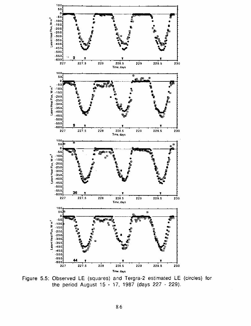
lOO
50:
O:
-5o:
E -loo:
-150:
-200:l,
,_ -250
-300
-350¢b
-400:"J -450:
-500:
, I | l , _ , ! , i n
• : :-
-550:
-600 ' 2 ,V , ,V , ,V
227 227.5 228 228.5 22g 229.5 230
"time, days
1001 . , . , , , . , . i ,
50_ o _ a
,oL=_. ; =,__,.........................,"_'¢_o ,_-.;oot" . •
•. -,soI _ . _ ._ : ..-2oo.I ® _ . _ . %
d
-250 _ • _o %
..o_ I-550J --600J .U , V .... V .... ¥ .
227 227.5 228 228.5 229 229.5 230
"lime, days
loo_
-50
-,so.] %, -.. % _ _a 2 [2°°:1 _ ¢ _ "o % _ F
_2S°:l % • %_ • • .." F_-3oo,] _ _ " A" k "_ _ !"= -_S°:l _ J_ __ ._ _ _ F_.-,oot _ -I_l' _ F3.4so I _ '_- F
-soot [-sso.j _ , . . F-800
227 227.5 228 228.5 22g 229.5 230
Time, clays
100
-50-100
"2°°:1 % ..= =,, _ ° % _ i
.4ood _ _" %,%o l3 .4so:l _, .,m !"
"s°°_l i-ssoJ 44 , , , I'-600
227 22_.s 2_8 22_.s 2_ 22_.s 230
l_me, days
Figure 5.5: Observed LE (squares) and Tergra-2 estimated LE (circles) for
the period August 15 - 17, 1987 (days 227 - 229).
_6

lO0
50
0
-50E .100:
_: -150:
g -2002f_
-250:
_. -3oo:-350,
0
_ -400-450
-500
-550
| - • - i , | i
no .,_ur • _
. ="°
%0
-6oo' 902 v v:_521_.221;.42_;.e'21;.e" 2;5 2_;.221;.421;.e'21;.e
Time, days
100 ' ' ' ' ' ' ' ' ' '
5O
0
_E -50-loo:
_ 15o:¢. -2oo:
.250;-3oo:
-r
-3501
__ -400,-450
-500
!17
=.. _, eo •!11 Olh-O I_ e
Oo=tin
-550 908 v v-600 . . - - "
!15 21;.2"21;.4"21;.6 21;.8 2;6 "21;.2 21;.4 " 21;.6 " 216.8
Time, days
10o
50:
o:-501
'_E -100,
-150,
-200
-250
.= .3oo"E -3500
-400"_ -450:
-500:
'17
• . * i | I - " •
=To e..
o',r o0 0
-55o: 936 _a-600: . . • _ .......
Time. days
100
50
0
-so:'_E .100:
_" -15o:
-_ -2oo:
_- -250:
:_ -3oo."E -350.
__ -400.°450
-500
-550
_-_ _=-==e •
=='.. !;,_,," ==
944 v-600 . . - .... "
Time, days
Figure 5.6: Observed LE (squares) and Tergra-2 estimated LE (circles) forthe period August 3 - 4, 1989 (days 215 - 216). Data wereavailable only for day 216 at sites 936 and 944.

Tergra-2 estimates of LE during the two 1987 periods were more
accurate than those of the 1989 period at each flux station. Soil water
potentials during 1989 were substantially lower than those observed in
1987 (Table 5.3). While the rms error ranged between 37 and 63 W m -2
for the two wetter periods, the rms error for the 1989 simulations ranged
between 62 and 107 W m -2 (Table 5.4). Some of the smallest rms error
values for Tergra-1 were observed using the 1989 data. As will be
discussed later, this may not have reflected a superior representation of
conditions at this time period by Tergra-1, but may be attributable to
compensating errors.
An examination of the daily course of modeled and observed LE for the
two 1987 periods (Figures 5.4 and 5.5) reveals that most of the Tergra-2
model error tended to be associated with simulations close to solar noon.
A consistent overestimation/underestimation of LE at this time was not
discernable in an intersite comparison of the model results. In contrast,
Tergra-1 consistently overestimated LE and this overestimation was not
confined to the midday period. This result could be expected, since
Tergra-1 includes a leaf water potential adjustment of rc that is specific
only to C3 plants. Stomatal closure of the Konza prairie C4 plants and the
associated reduction in transpiration would be initiated at a higher leaf
water potential than the corresponding value defined in Tergra-1.
In the results presented in Figures 5.4 and 5.5 there was no evidence of
a decrease in Tergra-2 accuracy as simulations progressed from the soil
moisture conditions defined at the start of each simulation period. It
would, however, be necessary to conduct tests of the model over more
extensive time periods to establish whether the soil moisture budgeting
and model accuracy were stable over time.
88

The diurnal patterns of estimated LE using Tergra-1 for sites 908 and
944 in 1989 are given in Figure 5.7.
100 ....... ' ' ' ' " "
o - - ,,,,p:=opL_=_=_ o="=I=I-soT- "-"=- "=g,._ = °=_'_='"49 _ o no_
.^^4 "11 "1o • o"uuu t o. • OD- 150,1 It" • •
-2ool ':l, . _°° "° 0_"-25o:I m - • eea nO-sooJ _ • '':_* "a' -=o
,,; %p-4oo.:i._ -,so.j
-500_
-550.]-6ooi 908 Ir Ir
_',s "21_.2"21_.,'21_._'2',_.8" 2;6 "2.,_.2"21_.4"2'_._'21_.B" 217Time, days
= - . . • . = - . = , =100
50,
O,
-50,
'¥ - 100,
-15o-200
_- -250
-300
:_ -350® -400
-450
-5oo:.sso:
rD
-6oo' 944 V
Time, days
Figure 5.7: Observed LE (squares) and Tergra-1 estimated (circles) LE for
sites 908 and 944 for the August 1989 simulation period.
Tergra-1 rms error values for these tests were notably smaller than those
obtained using Tergra-2. Comparing the results for the corresponding
sites using Tergra-2 (Figure 5.6), the most notable difference between the
estimates from the two models occurred at station 908. Tergra-1
estimates of LE were close to the observed values on both simulation days
89

for periods close to solar noon. The characteristic overestimation of LE
by Tergra-1 was still evident for simulated fluxes at times other than the
midday period. Estimates of LE using Tergra-2 at station 908 were
consistently less than the observed fluxes, except for the period up until
mid-morning and the period after mid-afternoon on the second simulation
day (day 216).
The location of sites 908 and 944 in 1989 were close to the
locations of sites 8 and 44 in 1987. Comparing observed LE values in
August 1987 with those observed in August 1989 at these sites, it is
apparent that there were similar magnitudes of LE at both times despite
large differences in soil water potential. The differences in fluxes at
midday were less than 25 W m-2 for both locations. At station 8 (908)
the soil water potential was -30 kPa in 1987 and -794 kPa in 1989 and at
station 44 (944) the corresponding soil water potentials were -89 kPa and
-698 kPa (Table 5.3). It would be expected that LE at the two sites for the
August 1989 period would be substantially less than that which was
observed. Since the soil moisture used in the model simulations was
measured at a depth of 10 cm, it may be argued that the plants were
responding to soil moisture conditions deeper in the soil profile. Jarvis
(1989) concluded that as stress sets in close to the soil surface, the
location of peak water uptake by plants shifts steadily down the soil
profile. Alternatively, there may have been local sources of LE that were
not responding to the average soil water content used in the model
calculations.
If it is assumed that the soil water potential or the parameterization of
the soils for this station was incorrect in the direction of greater soil
water stress, then the exclusively C3 parameterization of the leaf water
9O

potential stress index in Tergra-1 would tend to compensate for the
reduction in LE. It is notable that station 908 had the lowest ratio of
03:04 plants (0.18:0.82) of any of the sites at any of the three time
periods (Table 5.3). Thus, if soil water stress was greater than it should
have been, Tergra-2 would have been particularly sensitive to this error,
given the dominance of C4 plants at this station.
The introduction of a vapor pressure deficit stress factor to determine
actual canopy resistance did not have a major impact on the modeled LE.
In most cases, the increase in modeled canopy resistance above its
minimum value was caused by a reduction in leaf water potential.
5.3.5 Discussion
Modifications made to the canopy resistance component of the Tergra
model resulted in a model that was better suited to the simulation of LE
over the Konza prairie than the original model. Basing canopy resistance
on the NDVI in Tergra-2 makes the model more compatible with remotely
sensed data and more suitable for making estimates of spatial patterns of
LE. An added advantage of including the NDVI in the model is that it
provides a means for simulating the relationship between surface
temperature and the NDVI.
The evaluation of Tergra-2 accuracy in these tests needs to be made
in the context of the spatial variability of plant and soil variables that
characterize the Konza prairie. Reichman (1987) points to the large
species diversity that tends to occur on the shallow and rocky soils of the
Konza prairie and the occurrence of "specialist" plants on these soils.
Reichman also describes how forbs and shrubs are generally found in
9]

patches. Wetzel and Chang (1987) allude to the great variability in soil
characteristics commonly found in a single soil type, which can cause a
wide disparity in water content within a relatively small area. In the
Tergra model, variables such as soil water potential, rooting depth,
canopy height, and soil depth are represented as average values, whereas a
disproportionate contribution to the fluxes measured at a station may be
originating from isolated sources not characterized by mean conditions.
Attention should be given to structuring Tergra-2 to include measures of
variance in some of the input variables and parameters. It is also
recognized that the modified resistance component of Tergra-2 still may
not be fully representative of the processes operating in the Konza prairie
and additional modifications may be necessary.
While the modeled canopy resistance in Tergra-2 was generally
affected by leaf water potential and not vapor pressure deficit, field
studies conducted by Sellers et al. (1990) indicated that stomatal closure
of the plants in the Konza prairie was under the control of vapor pressure
deficit. These contrasting findings may be explained by considering the
correlation between leaf water potential and vapor pressure deficit. A
decrease in LE, caused by stomata closing in response to a reduction in
leaf water potential, may have reduced the vapor pressure at the bottom
of the atmospheric boundary layer (ABL) where measurements were made
for the FIFE. This is a basic premise in the explanation given by Bouchet
(1963) and others for the observed reciprocal relationship between actual
and potential evaporation. Thus, the role of vapor pressure deficit in
stomatal closure can not be regarded as independent of the leaf water
potential. Jarvis and McNaughton (1986) concluded that when plants are
grouped together, it can not be assumed that the vapor pressure deficit of
92

the air passing through the canopy is independent of a change in the
average stomatal resistance of the assemblage of plants. The degree of
coupling of the canopy with the atmosphere may also be a factor that
determines the relative importance of vapor pressure deficit in stomatal
closure. After reviewing many stomatal resistance formulations, Lynn
and Carlson (1990) were unable to understand the basis for a direct effect
of vapor pressure deficit on stomatal resistance. They concluded that it
is necessary to further examine the relationship between stomatal
resistance, transpiration, and leaf water potential, and there is a need to
clarify the vapor pressure deficit effect. The simulation results using
Tergra-2 support this conclusion.
The introduction of separate leaf water potential adjustments to canopy
resistance for C3 and C4 plants in Tergra-2 avoided the consistent
overestimation of LE evident for Tergra-1 simulations. The spatial and
temporal distribution of these two plant types is likely to become a
significant requirement when the modeling is extended to estimating the
spatial patterns of LE. Barnes and Harrison (1982) found that the 03:04
distribution in a Nebraska prairie was associated with soil type and
topographic position. The use of remote sensing and geographic
information system techniques may offer promise for mapping the 03:04
mix in the Konza prairie.
The mix of C3 and C4 plants in the Konza prairie may also provide a
partial explanation for the large LE observed at two sites under dry soil
moisture conditions and the underestimation of these fluxes by Tergra-2.
Jarvis and McNaughton (1986) suggested that when stomata start to close,
the relative allocation of transpiration between individual plants or plant
types (or leaves) should be considered, rather than the regulation of the
93

absolute amount from the stand as a whole. Thus, when 04 plants start to
close their stomata, the reduction in vapor pressure within the stand may
induce greater transpiration from the C3 plants (O'Toole and Tomar 1982).
This feedback is not represented in Tergra-2.
The simulation of canopy temperature in the Tergra model allows for
model calibration or verification over large areas when remotely sensed
observations of this temperature are available (Soer 1980). Although
Tergra-2 provided good estimates of LE at the sites used in this
experiment, a preliminary comparison of observed and estimated canopy
temperatures revealed overestimates of up to 6 K (Figure 5.8). The
observed canopy temperature values were obtained from the same
helicopter MMR data set that provided the reflected radiances used to
calculate the NDVI. Hall et al. (1990) reported similar differences
between observed radiometric temperatures and aerodynamic
temperatures that were calculated from observed sensible heat flux, air
temperature and wind speed data. Hall et al. suggested that the sensible
heat flux is driven by the gradient between the air temperature above the
canopy and the temperature within the canopy air space. The modeled
canopy temperature approximates this aerodynamic temperature, whereas
the temperature recorded by the radiometer may include thermal
contributions from bare soil, rock and dead plant material. The
directional properties of vegetation temperature (Kimes et al. 1980) and
the concept of aerodynamic temperature need to be researched further to
interpret modeled surface temperatures in terms of heat fluxes.
94

314
312O
310
308
0
0
0
0
000
O00D
0 o0 0
0 0
00
0
0
0 0
296
'O294
294 296 298 300 302 304 306 308 310 312 314
ESTIMATED CANOPY TEMPERATURE, K
Figure 5.8: Observed canopy temperature using a helicopter-mounted MMR
versus Tergra-2 estimates of canopy temperature.
5.3.6 Conclusions
Experimental tests of the Tergra-2 model were based on data
collected under wet to moderately wet and very dry soil moisture
conditions. Additional testing of the model under intermediate soil
moisture conditions is necessary and further testing under very dry
95

conditions may lead to modifications that make the model more suitable
to water-stressed conditions. Combining the Tergra model with a soil
evaporation routine should improve the accuracy of the model and would
allow it to be used in situations where vapor fluxes are not almost
exclusively attributable to transpiration. There are also broader research
questions that need to be addressed, such as developing techniques to
represent the spatial variability of soil and plant variables in SPA models,
the feedback between transpiration and stomatal functioning, the
redistribution of transpiration when certain species (for example, C4
plants) reduce their transpiration and the relationship between modeled
and observed canopy temperatures.
The determination of canopy resistance from a spectral vegetation index
and the stresses leading to stomatal closure need to be investigated
further. The empirical canopy resistance-NDVI relationship used in
Tergra-2 may only be suited to conditions observed during FIFE 1987 and
FIFE 1989.
96

6. MODELING LARGE AREA LE FLUXES AND TS
6.1
During the development and testing of Tergra-2, efforts were also
made to couple the model to a GIS so that the model could be used to
simulate spatial patterns of LE and Ts over the entire FIFE site. The
primary focus was on LE since modeled Ts was likely to differ
substantially from radiometric temperatures. However, it was still
anticipated that there would be a systematic agreement between the
modeled and observed Ts across the FIFE site. This attempt to scale the
modeling procedures to the scale of the FIFE site necessitated the use of
satellite data and the Thematic Mapper (TM) and AVHRR systems were
used in the analyses. Since a soil evaporation routine had not been
included in the modeling scheme, tests were conducted on days when
surface soil moisture content was minimal and soil evaporation could be
assumed to be a minor contribution to total LE flux.
6.2 Study Ob!ectives
A general goal of this project was to develop a procedure to
estimate regional LE fluxes using thermal infrared and reflected
shortwave radiation data from a system such as the AVHRR. The extension
of the Tergra-2 model from a simulator of LE and Ts at a single location to
a procedure for estimating the spatial patterns of these variables was in
keeping with this goal. The spatially explicit Tergra-2 model (Tergra-
2.GIS) was designed to simulate LE and Ts at the spatial resolution of the
9"7

AVHRR sensor. A key component of the study was obtaining, interpolating
and estimating the spatially variable inputs and parameters for the model.
Once Tergra-2.GIS had been developed, the following research
questions were addressed:
1) How accurately can Tergra-2.GIS replicate the observed area averaged
LE and Ts of the FIFE site? The 15 x 15 km study site is treated as the
spatial resolution of interest for the model simulations.
2) How accurately can Tergra-2.GIS replicate the spatial pattern of LE and
Ts observed across the FIFE site?
3) Does the use of an area averaged SVI value at the AVHRR ground
resolution and the failure to address spatial heterogeneities at finer
spatial scales affect the accuracy of model predictions of LE and Ts? Over
many landscapes, the large AVHRR pixels are likely to average reflected
spectral radiances from a heterogeneous surface.
The averaging of land-surface characteristics (e.g., surface
conductance estimated from a SVI) may give rise to errors in the
estimation of LE. The latent heat flux process is acutely nonlinear so it is
important to consider land surface heterogeneities in LE models
(Dickenson et al. 1991). This process involves variables that can vary
widely over short distances (Wetzel and Chang 1988). Avissar (1991) has
demonstrated how mesoscale circulation models are sensitive to the
parameterization of intra-patch variability. The use of average parameter
values over large areas is often inappropriate and may lead to significant
errors in the prediction of latent heat flux (Wetzel and Chang 1987;
Wetzel and Chang 1988; Avissar 1991; Dickenson, Henderson-Sellers et al.
1991).
98

6.3 Methodoloav--v
Tergra-2.GIS was used to simulate the diurnal course of LE and Ts on
three days in 1987, June 4-6. AVHRR data were available on June 6 so
this became the primary day for evaluating model performance. Most of
the comparisons between observed and estimated quantities were made at
the time of the NOAA 10 satellite overpass. Spectral vegetation index
values required to determine minimum canopy resistance (i.e., rcm = 1/g'c)
were obtained using AVHRR and TM data. The AVHRR data were used to
determine the NDVI for each grid cell (1.3 x 1.3 km) covering the FIFE site.
The TM data were used with Tergra-2.GIS in two modes, the first mode
using the original 30 m resolution data to calculate LE and Ts for each 1.3
x 1.3 km grid cell. The histogram of SVI values for each grid cell was
divided into 10 classes (equal width) and the simulations executed using
the SVI from mid-points of each class. The average LE and Ts of each grid
cell was determined by weighting the modeled class values by the relative
frequency of TM pixels in each class. The second procedure ignored intra-
cell heterogeneity and used the average SVI from TM data for each cell to
calculate the two output variables.
An attempt was made to remove spatial auto-correlation from
output variables (Ts and LE) used in statistical analyses. Semi-variogram
analyses of the AVHRR thermal observations indicated that the lag in the
data corresponded to approximately 3.07 pixels. Consequently, every third
pixel was extracted from the 63 original grid cells to give a sample size
of 21 for model comparisons.
99

6.3.1 Research data
Satellite data
Level l a NOAA10 AVHRR data were acquired at 1536 (CDT) on June 6
over the FIFE site. The view angle for this location was 34.90o which
produced pixel size of approximately 1.3 km. A 9 x 7 pixel sub-scene
covering the FIFE site was extracted from the image and the NDVI and Ts
determined for each pixel. The split window technique was used to derive
apparent surface temperature while the dark object subtraction technique
was used to correct the red and near infrared bands for atmospheric haze
(cf. Section 2.3).
In order to address the third research question (effects of spatial
heterogeneity), it was necessary to obtain satellite data with a finer
spatial resolution than that of AVHRR. A Landsat TM image was acquired
over the FIFE site a week before the AVHRR image (May 28, 1987). It was
assumed that the change in SVI over this period was minimal. The Kauth-
Thomas "greeness" SVI was calculated for the study site using the TM data
and made available by the FIS. This image was co-registered to the
AVHRR image and all non-grassland pixels were masked from the TM sub-
scene.
Model inputs
The implementation of Tergra-2.GIS to estimate spatial patterns of
LE and Ts at the AVHRR ground resolution required spatially variable soil,
plant and atmosphere inputs. Soil parameters were estimated from the
1:18,000 general soil series map. Proportions of the various soil series in
each grid cell were determined for the estimation of average parameters.
l O0

Soil moisture characteristic curves were obtained for each soil type from
the FIS. Soil moisture characteristic curve parameters required for
Tergra were derived using the scheme described by Huygen (1978). A
summary of the Tergra-2.GIS soil parameters for the four major soil
series in the FIFE site are given in Table 6.1
Table 6.1" Tergra-2.GIS parameters for the four major soil series.
PARAMETER BenFIor Clime
THETAS 0.425
BL 0.286SR 0.320
D 1.178
DO 0.144
RD 9.028
513 0.042
AKO 0.370HCS 1.296
HCD 1.176
PSIA -14.648
PSIS -4.236
0 400
0415
0 370
1 230
0 107
12 1500 040
0 581
1.298
1.242
-15.108
-3.830
SOIL TYPE
Dwight
0.410
0.334
0.1801.280
0.247
5.263
0.039
0.171
1.403
1.344
-17.064
-3.129
Tully
0.400
0 1550 000
1 300
0 166
7 831
0 029
0 2321 288
1 226
-13.445
-3.834
THETAS - saturated volumetric water content (-)
BL - pore size distribution factor (-)
SR - rest saturation (-)
D - density of soil (kg.m-3)
DD effective rooting depth (m)
RD root density resistance factor (m)
SO - volume fraction of soil organic components (-)AKO saturated hydraulic conductivity (m.s -1)
HCS - heat conductivity of saturated soil (W.m-I.K -1)
HCD - heat conductivity of dry soil (W.m-I.K -1)
PSIA - air entry value of soil (Pa)
PSIS - soil water pressure (Pa)
lO1

Spatial patterns of soil moisture content on June 4 were obtained
for each grid cell using the maps developed by Peck (1993). These maps
were constructed using airborne gamma radiation, gravimetric, neutron
probe and microwave radiometer (PBMR) measurements (see Appendix 1).
Soil density, organic matter fraction, saturated hydraulic conductivity and
texture were obtained from the FIS.
Numerous vegetation parameters had to be interpolated from
measurements made at the individual flux towers or other point locations
(e.g., 03:04 ratio, canopy height). Rooting depth was assumed to be equal
to the soil depth. Maximum canopy conductance (g'c)was estimated from
a SVI. The relationship between g*c and the Kauth-Thomas GN is given by
Sellers et al. (1990). A separate expression had to be developed for the
NDVI based on AVHRR data. The red and near infrared radiances were
interpolated for each flux station using the AVHRR pixel values and then
used to calculate the NDVIs for these stations. In order to obtain an
equation similar to Equation 5.7 to estimate g'c, the station values of
dg*c/dKpar were regressed on these NDVI values to give the following
expression:
dg*c/dKpar = 0.203 NDVI 0.073 (r 2 = 0.887) (6.1)
6.3.2 Modeling area averaged LE and Ts
The average LE for the FIFE site on each of the three study days
(June 4, 5 and 6) was obtained by averaging observed values from all flux
measurement stations. A comparison between the diurnal course of
observed and estimated LE using Tergra-2.GIS and AVHRR NDVI, TM Kauth-
1 02

Thomas GN (GN1) and the average Kauth-Thomas GN (GN2) for each cell, is
given in Figure 6.1. A summary of observed and estimated LE at three
times on June 6 is given in Table 6.2.
50 o , . m • * • ...... * ,
O. L .........................w ..............• ........................._ ............."it ..................
o" ° o _ _..loo • a _l o,
o o.15o 'i • "_ 0
"" o o i_ "+= *_
._o ,. " e,, _ =o o il =
-- in, • "t" uu.{,-z_u u o ._
| • • o ^ s q
tl • o e *
.oot v v ¥t-450_
216.2216.5216.1] 217 217.2217.5217.8 218 218.2218.5218.8
Juhan Day
Figure 6.1: Comparison of observed (o) and modeled LE using the AVHRR
NDVI (o), TM Kauth-Thomas GN (n) and the average Kauth-
Thomas GN (+).
Table 6.2: Comparison at three times on June 6, 1987 of observed LE (Obs)
and estimated LE using Tergra-2.GIS and AVHRR NDVl, TM
Kauth-Thomas GN (GN1) and the average Kauth-Thomas GN
(GN2) for each cell.
LE
TIME
10h45 13h45 16h45
Obs -317.6 -424.7 -282.8
NDVI -341.9 -405.3 -329.2
GN1 -333.8 -405.3 -329.2
GN2 -316.7 -387.9 -314.2
103

Estimates of area averaged site LE using Tergra-2.GIS were accurate
throughout the simulation period, regardless of the SVI approach used in
the model. The results given in Table 6.2 indicate that there may be a
tendency for model predictions using the AVHRR NDVI to be slightly less
accurate after mid-day with errors approaching 80 W m -2. Clearly, the use
of a mean Kauth-Thomas GN gives essentially the same results as the high
spatial resolution approach (GN2) and the additional computational time
was not justified.
Model estimates of area average site Ts on June 6 were less
accurate than estimates of LE (Table 6.3). As expected, the model
underestimated Ts as had been found in the original model evaluations at
individual flux stations (Chapter 5). The Terga-2.GIS model also reduced
the intra-site variability in Ts, with the coefficient of variation for
modeled values being half that of the observed values (Table 6.3). The
three different SVI approaches did not have a substantial effect on
estimated Ts with mean values being within 0.8 K of each other.
Table 6.3: Mean and coefficient of variation for observed Ts and
estimated Ts using Tergra-2.GIS and AVHRR NDVI, TM Kauth-
Thomas GN (GN1) and the average Kauth-Thomas GN (GN2) foreach cell.
MEAN (K) CV
Observed 305.3 0.4
Ts(NDVI) 302.6 0.2
Ts(GN2) 302.6 0.2
Ts(GN1) 301.8 0.2
! O4

6.3.3 Modeling spatial patterns of LE and Ts
The modeled LE at each of the flux measurement stations was
estimated by interpolating values from the grid of modeled values. These
interpolated LE values were, however, found to be substantially different
from the modeled values regardless of the SVI approach that was used in
Tergra-2.GIS. An example of the discrepancy between observed and
estimated LE at the flux measurement stations is illustrated in Figures
6.2 and 6.3.
-340
-360
-380
-4OO
_E -420
-440uJ._J
-460
-480
-500
-520
I • I I •
[] •
[] •
. • J • ! -
[]
• • • •
[] n[] O
[]
8 10 12 14 18 20 22 24 36 44
STATION
Figure 6.2" Observed (square) and estimated LE (circle) at 10 flux
measurement stations on June 4, 1987. LE modeled using
AVHRR NDVI.
l 05

While the model may not have captured the spatial dynamics in variables
controlling LE, it is also likely that the interpolation approach for
estimating point LE fluxes from the grid values was inappropriate. Fluxes
observed at the measurement stations were local fluxes controlled by
features within approximately 200 m of the flux towers (approximate
fetch). The large grid cell size (1.3 x 1.3 km) and the averaging of model
variables to simulate fluxes at this resolution, may also have suppressed
spatial variability in LE. While the observed range in station-to-station
LE approached 165 W m -2 at 1345 CST on June 4, the modeled cell-to-cell
range was approximately 65 W m -2. This reduction in variability with
increase in modeled ground area would be expected since the modeled LE
values would all approach a regional mean as the ground area increased.
-340,
-360,
-520-520 -500 -480 -460 -440 -420 -400 -380 -360 -340
OBSERVED LE (W rn"2 )
Figure 6.3" Observed versus estimated LE at the flux measurementstations on June 4, 1987. LE modeled using AVHRR NDVI.
1 06

More appropriate tests of the spatial patterns of simulated LE using
Tergra-2.GIS may incorporate fluxes observed from aircraft However, a
more pressing need is to include a soil evaporation sub-routine.
The comparison between modeled Ts and values determined from the
AVHRR data on June 6 revealed the expected systematic underprediction of
Ts. The relationship between observed and estimated values using the
three SVI approaches in the model are illustrated in Figure 6.4. The
scatterplots were similar for the three approaches and the relative
magnitude of underestimation of Ts appeared to increase with an increase
30,t • /
.t'/
3o4303
in observed Ts
301 302 303 304 305 306 307 308
NDVI-MODELEDSURF.TEMP.(K)
308. , /
_;307 e e /:S306 •
_3os IPsto _
•_3o_303
30Z
301301 302 303 304 305 306 307 308
GN--MODELEDSURF.TEMP. (K)
... 3o81
_ 306.
_305
._304
303
302;
301,301 302 303 304 305 306 307 308
AVE. GN-MODELEDSURF.TEMP.
.,,'."/
UFigure 6.4: AVHRR derived surface temperature (June 6, 1987) versus
surface temperature modeled using three different spectral
vegetation index approaches in Tergra-2GIS
107

6.4 Conclusions
Modelling spatial patterns of LE at AVHRR ground resolution using
remotely sensed SVI and soil moisture inputs was more accurate than the
modeling of Ts. The inclusion of a soil evaporation sub-model should
improve estimates of LE and make the model better suited to a wide range
of cover and soil moisture conditions. The sub-grid cell spatial
heterogeneity of the SVI, and hence rcm, did not have a significant effect
on the estimated LE or Ts.
108

7. CONCLUSIONS
A combination of empirical and modeling studies were conducted to
develop an understanding of the Ts-NDVI relationship in terms of energy
exchange processes. Procedures to estimate large area LE fluxes using
these combined observations were investigated using data collected from
a variety of sensors and platforms. While conclusions of the research
have been summarized at the end of each section or chapter, the following
general observations may benefit related studies that are conducted in the
future:
1) Simple atmospheric correction routines, such as the split window
technique Price (1984), darkest object subtraction technique (Chavez
1989) or the procedure described by Hall (1991), are valuable procedures
for the operational use of satellite data for energy balance studies.
2) Fractional vegetation cover is a major determinant of the thermal
response of grassland landscapes and this fraction is quantified by
spectral vegetation indices. This is the underlying cause of the widely
observed linear relationship between spectral vegetation indices and Ts.
Consequently, the variations in the Ts-NDVI relationship at large NDVl
values is more likely to be diagnostic of plant water stress than
variations associated with small NDVI values where Ts is largely
controlled by bare soil conditions.
3) It is unlikely that the slope (or intercept) of the Ts-NDVI regression
line will be useful as a direct indicator of LE fluxes due to the large
influence of terrain, surface cover conditions and management treatment
on the relationship. However, a significant relationship between the
regression slope and ground heat flux was observed.
109

4) Surface soil moisture conditions appear to be an important
determinant of the relationship between Ts and the NDVI at the local scale
(areas surrounding individual flux stations) or regional scale (AVHRR
coverage of loo latitude by 2oo longitude).
5) Terrain-induced variations in insolation (at the time of the
radiometric data collection) did not appear to affect the Ts-NDVI
regression characteristics.
6) The use of thermal infrared data and spectral vegetation indices in
soil-plant-atmosphere (SPA) models appears to be more promising for
surface energy balance studies than the analysis of Ts-SVI relationships.
However, the utility of remotely sensed surface temperatures over
incomplete vegetation canopies is still uncertain given that sensible heat
flux is controlled by aerodynamic temperature.
7) Techniques for estimating spatial patterns of soil moisture will be
critical for advances to be made in predicting spatial patterns of energy
fluxes using SPA models and remotely sensed data.
8) While the use of SVIs to estimate area averaged canopy conductances
is valuable for applying SPA models over large areas, estimating
evaporative contributions from the underlying soil is a source of
considerable uncertainty in modeling LE fluxes.
9) Vegetation composition, particularly the C3:C4 ratio, can not be
ignored in SPA models. Furthermore, landscape heterogeneity including
soil moisture, may explain the observed discrepancies between observed
and modeled area averaged LE fluxes.
The use of spectral vegetation indices to estimate minimum canopy
resistance over large areas for SPA models is promising. The relationship
between spectral indices and the resistance may vary with vegetation
l lO

type or season and these relationships need to be investigated further.
The development of procedures to convert minimum canopy resistance to
actual resistance needs to be a priority if this approach to modeling
evaporation is to be pursued.
It is clear from the studies summarized in this report and numerous
other investigations that radiative surface temperature deviate from the
effective surface temperature (aerodynamic temperature) controlling
sensible heat flux (Huband and Monteith 1986; Vining and Blad 1990; Lloyd
et al. 1992). The grasses of the Konza Prairie do not provide complete
canopy coverage so differential soil and vegetation heating will have to be
considered if thermal emissions and the residual energy balance approach
is to be used to estimate LE. Simple modifications to the bulk transfer
equation may be possible so that estimates of sensible heat flux are made
with acceptable accuracy (Stewart 1993). The observed difference
between radiative and aerodynamic surface temperatures has generally
been explained in terms of the differential heating of exposed soil and
vegetation elements. Therefore, it may be expected that measures of
fractional vegetation cover, such as the NDVI, would be useful for
estimating empirical corrections to the bulk heat transfer equation.
Improved large area energy balance models will need to explicitly
deal with landscape heterogeneity at a number of scales. Spatial
variations in vegetation cover type and composition (particularly C3:C4
ratios), management treatment, soil moisture and terrain may control
fluxes to a greater or lesser extent depending on the scale of observation.
The use of high spatial resolution remotely sensed data (e.g., NS001,
SPOT) should be included in future studies that address the problems of
heterogeneity and scaling.
Ill

REFERENCES
Asrar, G., T. R. Harris and R. L. Lapitan. 1988. Radiative surface
temperatures of burned and unburned areas in a tallgrass prairie.
Remote Sensing of Environment 24: 447-457.
Asrar, G., R. B. Myneni, Y. Li and E. T. Kanemasu. 1989. Measuring and
modeling spectral characteristics of tallgrass prairie. Remote
Sensing of Environment 27: 143-155.
Asrar, G., R. L. Weiser, D. E. Johnson, E. T. Kanemasu and J. M. Killeen. 1986.
Distinguishing among tallgrass prairie cover types from
measurements of multispectral reflectance. Remote Sensing of
Environment 19: 159-169.
Avissar, R. 1991. A statistical-dynamical approach to parameterize
subgrid-scale land-surface heterogeneity in climate models. Surveys
in Geophysics 12: 155-178.
Barnes, P. W. and A. T. Harrison. 1982. Species distribution and community
organization in a Nebraska sandhills mixed prairie as influenced by
plant/soil-water relationships. Oecologia 52: 192-201.
Bouchet, R. J. 1963. Evapotranspiration Reelle et Potentielle, Signification
Climatique. Proceedings of the International Association of
Scientific Hydrology 62: 134-142.
112

Carlson, T. B., E. M. Perry and T. J. Schmugge. 1990. Remote estimation of
soil moisture availability and fractional vegetation cover for
agricultural fields. Agriculture and Forest Meteorology 52: 45-69.
Carlson, T. N., J. K. Dodd, S. G. Benjamin and J. N. Cooper. 1981. Satellite
Estimation of the Surface Energy Balance, Moisture Availability and
Thermal Inertia. Journal of Applied Meteorology 20: 67-87.
Chavez, J., P.S. 1988. An improved dark-object subtraction technique for
atmospheric scattering correction of multispectral data. Remote
Sensing of Environment 24: 459-479.
Chavez, J., P.S. 1989. Radiometric calibration of Landsat Thematic Mapper
multispectral images. Photogrammetric Engineering and Remote
Sensing 55(9): 1285-1294.
Choudhury, B. J. and S. B. Idso. 1985. An Empirical Model for Stomatal
Resistance of Field-Grown Wheat. Agriculture and Forest
Meteorology 36: 65-82.
Choudhury, B. J. and S. B. Idso. 1985. Evaluating Plant and Canopy
Resistance of Field Grown Wheat from Concurrent Diurnal
Observations of Leaf Water Potential, Stomatal Resistance, Canopy
Temperature, and Evapotranspiration Flux. Agriculture and Forest
Meteorology 34: 67-76.
113

Choudhury, B. J., S. B. Idso and R. J. Reginato. 1986. Analysis of a
Resistance-Energy Balance Model for Estimating Daily Evaporation
from Wheat Plots Using One-Time-of-Day Infrared Temperature
Observations. Remote Sensing of Environment 19: 253-268.
DeVries, D. A. (1975). Heat Transfer in Soils. Heat and Mass Transfer in the
Biosphere. Part 1: Transfer Processes in the Plant Environment.
Washington, D.C., Scripta. 5-28.
Dickenson, R. E., A. Henderson-Sellers, C. Rosenweig and P. J. Sellers. 1991.
Evapotranspiration models with canopy resistance for use in climate
models, a review. Agricultural and Forest Mteorology 54: 373-388.
Dubayah, R., J. Dozier and F. Davis. 1989. The distribution of clear-sky
radiation over varying terrain. International Geoscience and Remote
Sensing Symposium, Vancouver.
Feldman, D. S., J. Gagnon, R. Hofmann and J. Simpson (1987). StatView IL
Berkeley, Abacus Concepts.
Fisher, M. J., D. A. Charles-Edwards and M. M. Ludlow. 1981. An analysis of
the effects of repeated short-term w ater deficits on stomatal
conductance to carbon dioxide and leaf photosynthesis by legume
macroptilium stropurpureum cv. sirato. Autralian Journal of Plant
Physiology 8: 347-357.
114

Goward, S. N., G. D. Cruickshanks and A. S. Hope. 1985. Observed Relation
Between Thermal Emissions and Spectral Radiance from a Complex
Vegetated Landscape. Remote Sensing of Environment 18: 137-146.
Goward, S. N. and A. S. Hope. 1986. Measurement of evapotranspiration
with combined multispectral solar reflective and thermal infrared
radiance observations. First ISLSCP Field Experiment (FIFE) proposal
submitted to: National Aeronautics and Space Administration.
Goward, S. N. and A. S. Hope. 1989. Evapotranspiration from Combined
Reflected Solar and Emitted Terrestrial Radiation: Preliminary FIFE
Results from AVHRR Data. Advances in Space Research 9(7):
239-249.
Gurney, R. J., J. P. Ormsby and D. K. Hall. 1983. A Comparison of Remotely
Sensed Surface Temperature and Biomass Estimates For Aiding
Evapotranspiration Determination in Central Alaska. Permafrost:
Fourth International Conference, Proceedings, National Academy
Press, Washington, D. C.
Hall, F. G., D. E. Strebel, J. E. Nickeson and S. J. Goetz. 1991. Radiometric
rectification: Toward a common radiometric response among
multidate, multisensor images. Remote Sensing of Environment 35:
11-27.
115

Hall, F. G., P. J. Strebel, E. T. Kanemasu, R. D. Kelly, B. L. Blad, B. J. Markham,
J. R. Wang and F. Huemmerich. 1990. FIFE, First ISLSCP Field
Experiment: Results Overview. Symposium on FIFE, Anaheim, CA,
American Meteorological Society, Boston, MA.
Holben, B. N. and C. O. Justice. 1980. The Topographic Effect on Spectral
Response from Nadir-Pointing Sensing. Photogrammetric Engineering
and Remote Sensing 46(9): 1191-1200.
Hope, A. S. 1992. Monitoring ecosystem response to global change: high
spatial resolution data. Symposium on Anticipated Effects of a
changing Global Environment on Mediterranean-Type Ecosystems,
Valencia, Spain, (Proceedings in Review).
Hope, A. S., S. N. Goward and D. E. Petzold. 1988. Tersail: A Numerical Model
for Combined Analysis of Canopy Bidirectional Reflectance and
Thermal Emissions. Remote Sensing of Environment 26: 287-300.
Hope, A. S. and T. P. McDowell. 1990. The use of remotly sensed surface
temperature and a spectral vegetation index for evaluating heat
fluxes over the Konza prairie. Proceedings of Symposium on the First
ISLSCP Field Experiment (FIFE), Anaheim, CA., American
Meteorological Society.
116

Hope, A. S. and T. P. McDowell. 1992. The relationship between surface
temperature and a spectral vegetation index of a tallgrass prairie:
effects of burning and other landscape controls. International
Journal of Remote Sensing 13(15): 2849-2863.
Hope, A. S., D. E. Petzold, S. N. Goward and R. M. Ragan. 1986. Simulated
Relationships Between Spectral Reflectance, Thermal Emissions and
Evapotranspiration of a Soybean Canopy. Water Resources Bulletin
22:1011-1019.
Huband, N. D. S. and J. L. Monteith. 1986. Radiative surface temperature
and energy balance of a wheat canopy. I. Comparison of radiative
and aerodynamic canopy temperature. Boundary-Layer Meteorology
36: 1-17.
Huete, A. R., R. D. Jackson and D. F. Post. 1985. Spectral response of a plant
canopy with different soil backgrounds. Remote Sensing of
Environment 17: 37-53.
Hulbert, L. C. 1969. Fire and litter effects in undisturbed bluestem prairie
in Kansas. Ecology 50: 874-877.
Huygen, J. 1978. An improved method for the definition of soil moisture
parameters used in the Tegra model. Tellus Newsletter, 6. Ispra,
Italy, Commmission of the European Communities, Joint Research
Center. 3:1-6.
117

Huygen, J. and P. Reiniger (1977). A sensitivity analysis of the Tegra
model for the conditions of the grendon test site. Ispra, Italy,
Commission of the European Communities, Joint Research Center.
Jarvis, N. J. 1989. A simple empirical model of root water uptake. Journal
of Hydrology 107: 57-72.
Jarvis, P. G. 1976. The interpretation of the variation in leaf water
potential and stomatal conductance found in canopies in the field.
Phil. Transactions of the Royal Society, London, B. 273: 593-610.
Jarvis, P. G. and K. G. McNaughton. 1986. Stomatal control of transpiration:
Scaling up from leaf to region. Advanced Ecological Research 15: 1-
49.
Kidwell, K. B. 1986. NOAA Polar orbiter guide. Washington, D.C., National
Oceanic and Atmospheric Administration , National Climate Center.
Kimes, D. S., S. B. Idso, J. Pinter P.J., R. J. Reginato and R. D. Jackson. 1980.
View angle effects in the radiometric measurement of plant canopy
temperatures. Remote Sensing of Environment 10: 273-284.
Knapp, A. K. 1984. Post-Burn Differences in Solar Radiation, Leaf
Temperature and Water Stress Influencing Production in a Lowland
Tallgrass Prairie. American Journal of Botony 71(2): 220-227.
118

Kondratyev, K. (1969). Radiation in the Atmosphere. New York, Academic
Press.
Kustas, W. P., R. D. Jackson and G. Asrar (1989). Estimating surface
energy-balance components from remotely sensed data. Theory and
Applications of Optical Remote Sensing. New York, John Wiley and
Sons. 604-627.
Laliberte, G. E., R. H. Broods and A. T. Corey. 1968. Permeability calculated
from desaturation data. Journal of Irrigation and Drain Diversion,
ASCE 94: 57-71.
Lloyd, C. R., J. H. C. Gash and M. V. K. Sivakumar. 1992. Derivation of the
aerodynamic roughness parameters for a Sahelian sanannah site
using the eddy correlation technique. Boundary-Layer Meteorology
58: 261-271.
Ludwig, J. A. and J. F. Reynolds (1988). Statistical Ecology. New York, John
Wiley and Sons.
Lynn, B. H. and T. N. Carlson. 1990. A stomatal resistance model
illustrating plant vs. external control of transpiration. Agriculture
and Forest Meteorology 52: 5-43.
Nemani, R. R. and S. W. Running. 1989. Estimation of Regional Surface
Resistance to Evapotranspiration from NDVI and Thermal-IR AVHRR
Data. Journal of Applied Meteorology 28(4): 276-284.
119

Nieuwenhuis, G. J. A., E. H. Smidt and H. A. M. Thunnissen. 1985. Estimation
of Regional Evapotranspiration of Arable Crops from Thermal
Infrared Images. International Journal of Remote Sensing 6:
1319-1334.
Nieuwnhuis, G. J. A. and W. Klaasen (1978). Estimation of Regional
Evapotranspiration from Remotely Sensed Crop Surface Temperature.
Ispra, Italy, Commission of the European Communities, Joint
Research Center.
O'Toole, J. C. and V. S. Tomar. 1982. Transpiration, leaf temperature and
water potential of rice and barnyard grass in flooded fields.
Agricultural and Forest Meteorology 26: 285-296.
Pallaconi, F. 1988. Jet Propulsion Laboratory, Pasadena, CA.
Peck, E. L. and A. S. Hope. 1993. Spatial patterns of soil moisture for the
FIFE study area derived from remotely sensed and ground data.
Journal of Geophysical Research. Submitted:
Polley, H. W., J. M. Norman, T. J. Arkebauer, E. A. Walter-Shea, D. H. Greegor
Jr. and B. Bramer. 1992. Leaf gas exchange of Andropogon gerardii
Vitman, Sorghastrum nutans (L.) Nash in a tallgrass prairie. Jornal of
Geophysical Research 97(D17): 18,837-18,844.
120

Price, J. C. 1984. Land surface temperature measurements from the split
window channels of the NOAA-7 advanced very high resolution
radiometer. Journal of Geophysical Research 89(D5): 7231-7237.
Price, J. C. 1990. Using spatial context in satellite data to infer regional
scale evapotranspiration. IEEE Transactions on Geoscience and
Remote Sensing 28(5): 940-948.
Reichman, P. E. (1987). Konza Prairie: A Tallgrass Natural History.
Lawrence, KS, University Press of Kansas.
Ritjema, P. E. (1965). An Analysis of Actual Evaportanspiration.
Agricultural Research Report, Wageningen, The Netherlands, Pudoc.
107.
Roscoe, J. T. (1975). Fundamental Research Statistics for Behavioral
Sciences. New York, Holt, Rinehart and Winston.
Saunders, R. U. and K. T. Kriebel. 1988. An improved method for detecting
clear sky and cloudy radiances from AVHRR data. International
Journal of Remote Sensing 89: 7231-7237.
Schmugge, T. J., E. T. Kanemasu and G. Asrar. 1987. Airborne multispectral
observations over burned and unburned prairies. IGARSS'87
Symposium, Ann Arbor, MI, Institute of Electrical and Electronic
Engineers.
121

Sellers, P., M. Heiser, C. W. Walthall, F. Huemmerich, D. E. Strebel and F. G.
Hall. 1990. A Comparison of surface biophysical properties and
remotely sensed variables from FIFE. Symposium on FIFE, Anaheim,
CA, American Meteorological Society, Boston, MA.
Sellers, P. J. 1985. Canopy reflectance, photosynthesis and transpiration.
International Journal of Remote Sensing 8(6): 1335-1372.
Shawcroft, R. W., E. R. Lemon and D. W. Stewart. 1973. Estimation of Plant
Internal Crop Water Status from Meteorological and Plant
Parameters. Proceedings Uppsala Symposium, Plant Response to
Cimatic Factors, 449-459.
Sirkov, S. I. 1971. Computation of Solar Radiation Characteristics.
Jerusalem, Keter Press.
Soer, J. G. R. 1977. The Tegra model, a mathematical model for the
simulation of the daily behaviour of crop surface temperature and
actual evapotranspiration. Delft, The Netherlands, Netherlands
Interdepartmantal Working Community for the Application of
Remote Sensing Techniques. Publication 46: 44.
Soer, J. G. R. 1980. Estimation of regional evapotranspiation and soil
moisture conditions using remotely sensed crop surface
temperatures. Remote Sensing of Environment 9: 27-45.
122

Stewart, J. B. 1993. Radiative surface temperature derived sensible heat
flux for sparse prairie grass. American Geophysical Union Spring
Meeting, May 24-28, Baltimore, Maryland.
Vining, R. C. and B. L. Blad. 1990. Relationship Between Radiometric,
Aerodynamic and Kinetic Canopy Temperatures of Prairie Vegetation.
AMS Symposium on the First ISLSCP Field Experiment, Anaheim, CA.
Weiser, R. L., G. Asrar, G. P. Miller and E. T. Kanemasu. 1986. Assessing
grassland biophysical characteristics from spectral measurements.
Remote Sensing of Environment 20: 141-152.
Wetzel, P. J. and J. T. Chang. 1987. Concerning the relationship between
evapotranspiration and soil moisture. Journal of Climate and Applied
Meteorology 26: 18-27.
Wetzel, P. J. and J. T. Chang. 1988. Evapotranspiration from non-uniform
surfaces: a first approach for short term numerical weather
prediction. Monthly Weather Review 116: 600-621.
Whitehead, V. S., W. R. Johnson and J. A. Boatright. 1986. Vegetation
assessment using a combination of visible, near-IR, and thermal-IR
AVHRR data. IEEE Transactions on Geoscience and Remote Sensing
GE-24(1): 107-112.
Wilson, W. H. 1980. Solar ephemeris algorithm. Scripps Institute of
Oceanography, Visibility Laboratory, University of California.
123

APPENDICES
124

APPENDIX 1
SPATIAL PATTERNS OF SOIL MOISTURE FOR THE FIFE STUDY
AREA DERIVED FROM REMOTELY SENSED AND GROUND DATA
EUGENE L PECK
Hydex Corporation, Vienna, Virginia
ALLEN S. HOPE
San Diego State University, San Diego, California
Paper Submitted To: Journal Of Geophysical Research
AI-I

SPATIAL PATTERNS OF SOIL MOISTURE FOR THE FIFE STUDY AREA DERIVED FROMREMOTELY SENSED AND GROUND DATA
EUGENE L, PECK
Hydex Corporation,Vienna, Virginia
ALLEN S. HOPE
San Diego University,San Diego, California
Soilmoisture observationswere made over the FIFE study area in1987
and 1989 using a variety of ground and airborne techniques. A
procedure is described for derivingspatialpatterns of soilmoisture bycombining these differentdata types. The spatialpatterns o_ soilmoisture are represented as both contour and grid values so that they
can be readilyincorporated in other FIFE studies. Two examples are
given that illustratethe utilityof these soilmoisture maps for remote
sensing and hydrometeorologicalstudiesover the FIFE study area.
INTRODUCTION
The First ISLSCP (International Satellite LandSurface Climatology Project) Field Experiment (FIFE)was conducted during the summer months of 1987 and1989 near Manhattan, Kansas, in support of an inter-
disciplinary experiment sponsored by the NationalAeronautics Space Administration (NASA). A majorobjective of FIFE is to develop methodologies forderiving quantitative information concerning land-surface climatological variables from satelliteobservations of radiation reflected and emitted by theearth. Information on the FIFE experiment and on
analyses and results of many of the scientificinvestigations are presented in the special FIFE issueof the Journal of Geophysical Research [AGU 1992].
Knowledge of the temporal and spatialvariations in soil moisture is required for many FIFE
investigations. To provide information for this need,seven ground based and remote sensing soil moisturedata collection experiments were conducted. Three ofthese soil moisture investigations provided dailyestimates for large portions of the FIFE research area
(15 by 15 km). These are the Pushbroom microwaveradiometer (PBMR) system operated by NASA [Wanget al., 1990], the airborne gamma radiation system ofthe National Weather Service [Carroll et al., 1988], andthe application of a hydrologic model to Kings Creekbasin [Famiglietti et al., 1992]. In addition, in situmeasurements (gravimetric) were made daily by theFIFE staff at a network of field experiment sites. Thesoil moisture values obtained using the differentmeasurement procedures can not be compared
directly. To be of most value to other investigators, a
method of combining the information content o! thevaries soil moisture estimates and measurements is
required.The purpose of this study is to derive the
spatial patterns of daily soil moisture over the FIFEstudy area during the principle experimental periodsusing data collected from a variety of ground andairborne sources (gravimetric, neutron probe,microwave and gamma ray). The utility of the soilmoisture maps developed in this project is illustrated
using selected examples.
DATA SOURCES
CORE In Situ Ground Measurements
Ground soil moisture samples were collected
daily by the FIFE staff [Sellers and Hall, 1987; Sellersand Hall, 1989] at CORE sites (located at flux andautomatic meteorological measuring stations). Soilmoisture samples were obtained daily from five pointsat the CORE stations, one at the center of the site andfour at short distances along cardinal directions fromthe center. Soil samples for 0 to 5 cm and 5 cm to 10
cm soil depths were obtained at each of the fivelocations . The soil moisture values for the sampleswere determined by the gravimetric method (percent
per cky weight). Average values of soil moisture for the0 to 10 cm depth were computed.
Airborne Gamma Radiation Measurements
The National Weather Service airborne gamma
radiation system [Carroll el al., 1988] was used to
AI -2

J, . .....
_. I 2 "° _ '_ _ "% _ _ _ _' '_
.. _ _ _ _ _ _. -_ __ - _'_
,o o •
. ,_; ,, _ ,-,. _ _ _ _"
o
t_
\
AI-3
q
•, !
->.
,/
ca _
_ J
._
la_
oE
_ E
E o
e-
_E
__>
._E
°_
X
._0,
measure soil moisture during FIFE 1987 and FIFE1989. Information on the locations of the 24 gammaradiation flight lines established and flown during FIFEfield experiments (19 flight lines in 1987 and 24 flightlines in 1989) and on the flight line sections established(portions of the flight lines) was presented by Peck etal. [1992]. Detailed information is available in the FIFE
Information System (FIS) located at the NASA, GoddardSpace Flight Center, Greenbelt, Md.
Measurements obtained by the airbornegamma radiation system along a flight line aremeasurements of the average soil moisture over anarea rather than along a single line. The airbornemeasurement of a flight line is assumed to measure awidth of approximately 305 meters across the line. Theaverage length of the 142 flight line sectionsestablished for the FIFE 24 flight lines is 1230 m. Thearea represented by an average section measurementof a flight line is 0.38 krn2 (1.23 km times 0.305 km).
The method for determining soil moistureestimates for sections of the flight lines from theradiation data collected by the airborne gamma flightswas presented by Peck, et al. [1990]. Soil moistureestimates for flight lines and for flight line sections, and800 individual in situ soil moisture measurements
(gravimetric method) obtained for calibration of theairborne gamma radiation flight lines are available in theFIS.
Neutron Probe Measurements
In situ measurements of soil moisture were
obtained by Ungar et al.[1992] duringFIFE 1987 using
neutron probes. Data from some of the access tubes
were averaged torepresent the soilmoisture along line
transects (e.g.,hillslope)and others were used to
determine the average soilmoisture at individualsites.
Information on the neutron probe measurements isgiveninthe FIS.
Microwave Radiometer (PBMR) Measurements
PBMR measurements were obtained prior to,during, and following the FIFE experiments by Wang etal. [1990]. Information on the PBMR flights and soilmoisture measurements is described in the FIS. The
PBMR flight lines had an west-east orientation duringthe 1987 experiment and a north-south orientationduring the 1989 experiment. Detailed information on
biomass and the spatial distribution of vegetation wereused in a model for computing soil moisture estimatesfor 1987 [Wang et al., 1990]. A simple method, usingonly ground soil moisture records, was used tocompute soil moisture estimates from the PBMR
measurements in 1989 [private communication].
Files of estimated soil moisture values,computed from the PBMR data, were provided by FISfor all days flights were flown during 1987 and 1989.These files consisted of percent average soil moisturevalues for pixels approximately 15 m by 15 m.
Hy_'ologic Model Values
A hydrologic model has been applied byFamiglietti et al. [1992] to the Kings Creek Basin forthe summer season of 1987. The Kings Creek Basin
is located in the center of the Konza research area (aresearch area operated by the Kansas State Universityand an important part of the FIFE study area). Daily soilmoisture estimates for the Kings Creek Basin from themodel study were provided in a digital format by EricWood for the periods June 3-4 and July 6-9, 1987(personal communication). Each pixel of the file has aresolution of 30 by 30 meters.
EVALUATIONS OF SOIL MOISTURE ESTIMATES
All available measurements of soil moisture
were considered for use in the analyses to producesoil moisture maps. The largest number of soilmoisture measurements for the Konza research area
where most of the FIFE studies were conducted, were
from the airborne gamma system. These remoteestimates were for flight lines, flight line sections, orcombination of sections. The flight line sectionsestimates in the Konza research area represent arealmeasurements of 0.30 km2 to 0.67 kin2 The second
largest number of soil moisture estimates available forthis area were those from the PBMR study. Arealvalues for any size area may be computed from the
PBMR data. Because of the greatest availability ofairborne gamma and PBMR data, an appropriate spatialresolution for deriving spatial patterns of soil moisturewas considered to be 0.5 km 2, about the average ofthe airborne gamma flight line sections in the Konzaresearch area.
Evaluations of the accuracy of themeasurements of soil moisture over the FIFE research
area have been reported by several FIFE investigators[Wang et al., 1990; Peck, et al. 1990; Peck andCarroll,1991]. Most of these studies have used the insitu ground soil moisture (CORE) measurements forthe evaluations since these data are considered to be
most accurate and are available for all days.The various measurements and estimates of
the soil moisture have different, and variable,relationships with the average soil moisture for a 0.5kin2 area. These relationships are discussed in thefollowing sections.
A1-4

MicrowaveVersusAirborneGamma and CORE Data
Peck and Carroll[1991]made a comparisonstudy of the soilmoistureestimatesby the airbornegamma techniquewith 1987 soilmoistureestimates(and a few 1989 estimates)obtainedwiththe PBMRsystem. The resultsof thisstudy found that theairbornegamma estimatescorrelatedwellwith theCORE data(averageerror3.1percentand a biasof0.1percent).The PBMR 1987 estimateswere found tohave an averageerrorof6.3percentand a biasof6.5percent. Most of the average errorand bias of thePBMR estimateswere a resultof a highbias(81o 9
percent)when thevolumetricsoilmoisturecontentwaslessthan 25 percent.The biaswas found tovary inrelationto ground conditions(e. g., littleor novegetationto highvegetationand grazedarea versusnon-grazedarea).No apparentbiaswas foundforthefew microwaveestimatesavailableatthattimefor1989.
Model EstimatesVersusGamma and CORE
Peck and Carroll[1992]compared averagesoilmoistureestimatesderivedfrom the hydrologicmodel
implemented by Famigliettiet al.[1992]with COREmeasurements and with airbornegamma estimates.Average dailysoilmoisturevalueswere computed forthe area measured by each sectionof the airbornegamma flightlinesover the Kings Creek basin byaveragingpixelvaluesfromthehydrologicmodel (using
the average of 11 data pointsacross the flightlinesection).
The studyfound thatthe CORE and airbornemeasurements duringJune and July1987 were wellrelatedand followedthe same temporalsoilmoisture
patternduringthe period.The soilmoisturevaluesforthe CORE and airbornegamma system decreasedduringthe fielddays in June 1987 and increasedapproximately6 percentby earlyJuly.The valuesfromthe hydrologicmodel outputcontinuedto decreasefrom earlyJune through July and did not properlyaccountforthe rainfallthatoccurredduringthe timebetween the June and Julyexperimentalperiods.
NeutronProbe VersusCORE Data
The neutron probe soilmoisture estimateswere limitedinnumber butwere inagreementwiththeCORE measurements as reportedby Ungar et el.
11992].
ANALYSES OF DATA
The resultsofthe previouscomparisonstudieswere used as a basisforexaminingrelationshipsamongthe soilmoistureestimatesfrom the varioussources
and determiningthe relationshipsof the in situsoilmoisturemeasurements withtheaveragesoilmoisturefora 0.5kin2. The method forhandlingeach ofthe
dflerentsetsofdataispresentedbelow:
Microwave PBMR Measurements
Average valuesforeach 0.5 kin2areawere
computed from the digitizedinformationfurnishedbythe FIS for the totalarea covered by the PBMRmeasurements forthreedays in1987 and threedaysin 1989. The number of 0.5 kin2 area values
computed for each day are given in Table I anddepended on the heightthatthe PBMR sensorswasflownand on theareacoveredby theflights.
TABLE 1. Number of 0.5 kin2 areas from PBMR
measurement system.
Number Number1987 ofareas 1989 ofareas
June 4 282 August4 190
July7 356 August7 640July9 360 August10 192
The computed average 0.5 kin2valueswerecompared with the dailymeasurements at COREstationslocated withinthe same 0.5 kin2areas.
Comparison foreightareas in1987 revealedthatthePBMR valuesaveraged5.47percentsoilmoisturelessthanthecorrespondingCORE values.A similarbias(-6.2 percent)was reportedby the Peck and Carroll[I991]comparisonstudyforthe 1987 fieldperiod.
The biasforthe1989 PBMR datafurnishedby
theFIS as compared withinsituCORE datawas foundtovaryovertheFIFE area.Comparisonoftheaverage1989 PBMR 0.5 kin2valuesfor 16 areas,when the
microwaveestimateswere lessthan25 percent,waspositive4.4percent. For fourotherareas,with1989PBMR microwaveestimatesgreaterthan25 percent,aminus biasof 4.8 percentwas observed. The biasseemed to be correlatedwiththe vegetationcoveroftheareas.
CORE Measurements
The CORE valueshave been consideredtobe the most reliableand most consistentset ofsoilmoisturemeasurements forthe FIFE researcharea.
As such,they have been used forcomparisonwithother measurements. However, CORE
measurements do not necessarilyrepresenttheaveragesoilmoistureforthesurrounding0.5kin2area.
A1 -5

Most CORE measurement locations are in
open, well exposed sites, and except for very wetperiods, the CORE measurements are lower than theaverage of soil moisture for the area surrounding thelocation. This was shown by Peck [1992] in the finalreport on the activities and results of the FIFE airbornegamma radiation studies.
Peck [1992] compared the measurements fora CORE station (site 906) located in an open site in theKonza research area with measurements along a north-south flight line. He found that the CORE value forAugust 5, 1989, was 6.5 percent lower than theaverage of 37 measurements along the flight line. Thevalues for three points with similar exposure near thestation had average soil moisture values within 1.0percent of the value at the station. The average valuefor nine points, including the three with exposuressimilar to the CORE site, along the flight line nearest thestation was 3.0 percent higher. For CORE locationsthat have open exposures, and the soil moisture valuesare less than 30 percent, the average value for the 0.5km 2 area centered at a CORE station has been
assumed to be 2.0 to 3.0 percent greater than that ofthe CORE station. For those few CORE sites in
protected locations, the reported soil moisture arebelieved to be more representative of the average overa 0.5 kin2 area.
Neutron Probe Measurements
For those locations in the Konza Research area
where neutron probe measurements were made alongspecific transects, the average of these measurementswere used in preparing the maps.
Hydrologic Model Estimates
Since the hydrologic model application during1987 did not adequately reflect temporal soil moisturechanges as indicated by CORE and airborne gammaradiation measurements these estimates were not used
in the soil moisture map analyses.
MAPS PREPARED
Soil moisture maps were analyzed for the 15days in 1987 and 1989 as shown in Table 2.
The CORE, airborne gamma radiation flight linesections, and the neutron probe soil moisture valuesfor each day were plotted on a base map (scale 1 to
24,000) using the ARC/INFO geographic informationsystem (GIS) at San Diego State University, San Diego,California. The average values for the 0.5 km2areas, ascomputed from the digitized files of the PBMRmeasurements, were also plotted on these base maps.
Using the plotted information, the differencesbetween the airborne gamma and PBMR soil moistureestimates could be easily observed. Having a personalknowledge of the entire FIFE research area was ofvalue in considering these average differences and
relating the variation of the differences to vegetativecover and land use. The differences between the
airborne gamma soil moisture estimates and thecomputed PBMR were considerably different for 1987than for 1989.
TABLE 2. Days soil moisture maps wereprepared
1 987 1989June 3 August 2June 4 August 4July 6 August 5July 7 August 6July 8 August 7July 9 August 8July 10 August 9
August 10
The computed soil moisture estimates fromthe PBMR digital files were extremely valuable fordefining the isolines for specific days, especially forareas where there were little or no other information.
The six days of PBMR values provided greatenhancement of the areal extent of information.
PBMR values were available within one day, for eachday maps were prepared.
The PBMR estimates were also valuable as a
check on a few of the gamma radiation values for thoselocations where access to the flight line was limited ornot permitted (e. g. flight lines KS110 and KSl13 inthe southwest portion of the FIFE research area). Forthese lines, even though the values for the entire
flight lines appeared to be reliable, the ground soilmoisture values were apparently not adequate toproperly calibrate the variation in soil moisture for allsections along the flight lines. For these flight lines,soil moisture values for some sections were found to
be consistently low, or high, whenever the measured
soil moisture for the flight line deviated considerablyfrom the value of the soil moisture for the day the flight
line was calibrated. On these same days, the valuesfor other sections of that flight line were found vary theopposite direction.
Isolines of equal 0.5 kin2 soil moisture values
were analyzed taking into account the results of thecomparison studies of the various soil moistureestimates and comparing the plotted values by subareas where the vegetative cover and or land use wasknown.
A1-6

DIGITIZED MAP DATA
The soil moisture isolines for the 16 maps were
digitized by the Geography Department of San DiegoState University. Files of the digitized isolines andcorresponding files of 0.5 km2 grid interpolated values
• for each day were prepared and have been submittedfor inclusion in the FIS. An example of a isoline mapand of 0.5 km 2 values on a 1.0 km grid are shown inFigure la and Figure lb, respectively.
UTILITY OF SOIL MOISTURE MAPS
The isoline and gridded soil moisture valuesprovide other scientists with daily soil moisture valuesthat have been developed using data from manysources but specific information of potential errors or
uncertainty is not provided. The primary advantage ofthe map and grid values is having a single value for alocation rather than a large number of values over thesurrounding area that are difficult to evaluate.Validation studies need to be continued. The followingtwo examples illustrate how the gridded soil moisturevalues can be used to investigate soil moisture
dynamics over the Konza study area or to assist with theinterpretation of other data sets.
A preliminary examination of the soil moisturegrid values has indicated their potential utility |orexplaining spatial variations in observed surfacetemperature. Hope and McDowell [1992] havedemonstrated that most of the variance in remotely
sensed surface temperatures over the Konza study sitecan be accounted for by variations in the normalizeddifference vegetation index (NDVI). These authors alsofound soil moisture measured at a depth of 25 ram,affected the relationship between these lwo variables.Reflected red and near infrared radiances and emitted
thermal radiances were collected using the NS001Thematic Mapper simulator on board the NASA C-130aircraft that was flown over the Konza study site onAugust 4, 1989. The spatial resolution of these data(12 m at nadir) were degraded to correspond to the soilmoisture grid illustrated in Figure lb. Thermal countsobtained from this sensor were regressed on thenormalized difference vegetation index (NDVI) that wascalculated using the red and near infrared radiances.This regression produced a coefficient of determinationof 0.678 which increased to 0.778 when soil moisture
was included in the analysis (n= 84). Figure 2aillustrates the observed relationship between surface
temperature and the NDVI while Figure 2b indicates therelationship between the regression residuals and thecorresponding grid soil moisture values.
The soil moisture maps also may be valuable forexamining soil moisture dynamics along transects
190
185,
180,
175,
170,
o 165,
16o,
155,-rv-- 150,
145,
140,
135.2
2O
go
gig
00 •
.2"5 .3"5 .4 .4"5 .5NDVI
Fig. 2a
- = . = . , .
15, •
100 • | •
S ee • • •i ° •
Oq_o •..,r. • :.=, • [
-1018 20 22 24 26 28 30 32 34 36
SOIL MOISTURE(%)
Fig. 2b
Fig. 2. 2a) Relationshipbetween NS001 surface
temperature and NDVI on August 4, 1989 and, 2b)
the relationship between surface temperature
residualsand corresponding gridsoilmoisture values.
corresponding to environmental or landscapegradients• Changes in soil moisture were examinedalong a north-south transect over a five-day dry-downperiod (August 5-9, 1989). This transect was locatedjust west of highway R-177. The changes in soilmoisture during the five day period are illustrated in
Figure 3. While the drying trend is evident in Figure 3,it is also apparent that the day-to-day pattern of soilmoisture content varies. The causes of this variabilityneed to be investigated further.
AI-7

36 h ,
34_
3z_
30
2B
26
24
22
20
16!43.18 43'.2 43.'22 43.'24 43[26 43[28 43'.3 43.32
• AUGUSTSB AUGUST6
AUGUST7O AUGUST8÷ AUGUST9
UTMNORTHING(XO.O000l)
Fig. 3. Soil moisture content along a north-south
gradientduring a fiveday dry-down period(5-9 August,1989).
Soil moisture is a major determinant of themagnitude of latent heat fluxes once the moisturestatus in the rooting zone falls below a critical threshold.
The relationship between the mapped soil moistureand observed latent heat fluxes was examined over the
same five-day period as the previous analysis. The ratioof daily latent heat flux to net radiation (evaporativefraction) was determined for sites 902, 908 and 910.The average evaporative fraction for each day was thenplotted against the average soil moisture obtained from
the 16 grid cells that covered the flux sites (Figure 4).As expected, the decrease in evaporative fraction overthis five day period appeared to relate directly to theobserved soil moisture status.
.75. - • , ...... , ,
.4 519.41
21 2'2 2"3 24 2'5 2'6 2'7 2_} 29
SOIL MOISTURE(%)
Figure 4. Relationship between the mean evaporativefraction from three flux sites (902, 908 and 910) and
the mean soil moisture from the 16 krn2 area containingthe sites (August 5-9, 1989)
CONCLUSION
Soil moisture data collected from a number of
different ground and airborne techniques can becombined to produce spatial patterns of soil moisturefor use in hydrologic and hydrometeorological studies.
The interpolation of soil moisture from contour to gridvalues is particularly useful for analyses that includeremotely sensed data in a raster format or for studies
along transects or gradients. Further research isrequired to quantify the accuracy of these spatialpatterns of soil moisture.
ACKNOWLEDGEMENTS
Thanks are extended to Eric Wood, Princeton
University,and to James Wang, NASA, for help withtheirsoilmoisture data. Our thanks alsotothe FIS staff
at NASA Goddard Space Flight Center, Fred
Huemmrich and JeffNewcomer, for providingdata andinformation. Special thanks are extended to Derren
Duburquet and Scott Augustine, Geography
Department, San Diego State University,for their
assistance with digitizingthe soilmoisture maps andcomputing the gridsoilmoisture values
REFERENCES
AGU, 1992. First ISLSCP Field Experiment (FIFE),Jour. of Geophys Res, Vol. 97. D17, Pages 18,345-18,371, November 30.
Carroll, T. R., E. L. Peck and D. M. Lipinski, 1988,Airborne Time-series Measurements of Soil MoistureUsing Terrestrial Gamma Radiation. Proc. Annual
Conf. American Soc. for Photogrammetry and RemoteSensing, St. Louis, MO, March 13-18. pp. 141-151.
Famiglieni, J. S., E. F. Wood, M. Sivapalan, and D. J.Thongs, 1992, A Catchment Scale Water Balance
Model for FIFE. Jour. of Geophys. Res., Vol. 97. D17,pp. 18,997-19,007, November 30.
Hope, A. S. and T. P. McDowell,1992. TheRelationship Between Surface Temperature and aSpectral Vegetation Index of a Tallgrass Prairie: Effectsof Burning and Other Landscape Controls. Int. J.Remote Sensing, Vol. 13, No. 15, pp. 2849-2863.
A1-8

Peck, E. L. 1992. Airborne Gamma RadiationMeasurements of Soil Moisture during FIFE; Activitiesand Results. Final Contractor Report in FIS, NASAContract NAS5-30959, Goddard Space Flight Center,Greenbelt, MD, April.
Peck, E. L. and T. R. Carroll, 1991, Comparison ofAirborne Soil Moisture Measurements by Microwaveand Gamma Radiation Techniques, Contract Report,
Hydex Corp., NASAIGFSC. Greenbelt, Md. 21 p.
Peck, E. L. and T. R. Carroll, 1992. Comparison ofAirborne Gamma Radiation Soil MoistureMeasurements with Hydrologic Model Output.Contractor Report in FIS, NASA Contract NAS5-30135, Goddard Space Flight Center, Greenbelt, MD.Dec., 1991, Revised Jan.
Peck, E. L., T. R. Carroll, and D. M. Lipinski, 1990,Airborne Gamma Radiation Soil Moisture
Measurements over Short Flight Lines. Preprint, Sym.on the First ISLSCP Field Experiment, Anaheim, CA,Amer. Meteorol. Soc., Boston, MA, Feb. 7-9. pp. 79-
84.
Peck, E L., T. R. Carroll and L. P. Lipinski, 1992.Airborne Soil Moisture Measurements for FirstInternational Satellite Land Surface Climatology
Program Field Experiment. FIFE Special Issue ofAmerican Geophysical Union, Jour. of Geophys. Res.,
Vol. 97. D17, pp. 18,961-18,967. Nov.,1992.
Seller, P. J. and F. G. Hall, 1987, FIFE Experiment Plan.NASA Internal Doc., 623, NASA/GSFC, Greenbelt, MD.
p. 394.
Seller, P. J. and F. G Hall, 1989, FIFE-89 ExperimentPlan. NASA Internal Doc., 623, NASA/GSFC,
Greenbelt, MD. p. 223.
Ungar, S. G,, R. Layman, J. E. Campbell, John Walshand Harlan J. McKim, 1992, Determination of Soil
Moisture Distribution From Impedance andGravimetric Measurements. Jour. of Geophys. Res.,
Vol. 97. D17, pp. 18,969-18,978, November 30.
Wang, J. R., Shiue, J. C., Schmugge, T. J., andEngman, E. T. 1990. The L-Band RadiometerMeasurements of FIFE Test Site in 1987-1989.
Preprints, Sym. on the First ISLSCP Field Experiment(FIFE), Anaheim, CA, Amer. Meteorol. Soc., Boston,MA, Feb 7-9. pp. 85-87.
A1-9

APPENDIX 2
A MODEL FOR COMPUTING IN-BAND REFLECTANCE DATA SETS
FROM DIGITAL SATELLITE IMAGE DATA
FREDERICK C. MERTZ AND SALLY J. WESTMORELAND
Photon Research Associates, San Diego, California
DOUGLAS A. STOW AND ALLEN S. HOPE
San Diego State University, San Diego, California
Proceedings, Workshop on Atmospheric Correction of Landsat
imagery, Torrance, CA, June 29-July 1. In Press
A2-1

A MODEL FOR COMPUTING IN-BAND REFLECTANCE DATA SETS
FROM DIGITAL SATELLITE IMAGE DATA
Frederick C. Mertz and Sally J. Westmoreland
Photon Research Associates, Inc.
10350 North Torrey Pines Court, Suite 300La Jolla. CA 92037-I020
Douglas A. Stow and Allen Hope
Department of Geography
San Diego State University
San Diego, CA 92182
1. INTRODUCTION
Measurement of objects or phenomena based on remotely sensed data are
affected by illumination geometry, viewing geometry, sensor characteristics, and
intervening atmosphere. Direct comparisons of remotely sensed data across time and
space require that collection dependent variations be minimized among observations.To minimize this variation, a robust model that reduces environmental and sensor
dependent artifacts must be developed. In this paper, we present a deterministic model
that computes in-band reflectance data from digital imagery by compensating for key
environmental and sensor dependent variables.
The model is currently applicable to satellite and aircraft imaging sensors in
the visible and short wave infrared region of the spectrum when the spectral responsefunction, sensor calibration coefficients, and the illumination and viewing geometries
are known. The model has been designed to provide rigorous and flexible atmospheric
correction capability coupled with ease-of-use. The model is robust in that it:
performs detailed atmospheric radiative transfer calculations for any atmospheric state,
spectral band, and sensor viewing geometry, rather than using a pre-computed database; models the atmosphere based on the base altitude of the site, and uses
background material reflectances extracted from a global data base to estimate thereflected earthshine; supports a user defned spectral response function as well as
providing a library of spectral filters for commonly modeled instruments; allows inputof user calibrated imagery in byte, short integer, and real data formats, as well as
supporting simple gain and offset calibration coefficients: models atmosphericvariations in atmospheric path length across the scene due to changes in solar andsensor zenith angles, and changes in surface altitude: compensates for changes insurface illumination effects due to variations in the orientation of a pixel by calculating
the vector between the sun and the surface normal vector; and treats the image as a
fiat plane at user specified altitude, ignoring atmospheric path length and surfaceorientation corrections when the user determines that the digital elevation data are of
questionable quality, or when the data are not available for a site.
2. THE MODEL
The model utilizes several separate computer programs integrated into a user-
friendly shell, RHO_DRIVER. The user interfaces with the model via a single input
file that contains the following parameters: date and time of image acquisition: scene
A2-2

center latitude and longitude; sensor latitude, longitude, and altitude; climatological
definition of the atmospheric state; sensor spectral response function; image calibration
coefficients: and file names for the geo-referenced image, a registered digital elevation
file, and a custom model atmosphere file. For each of the separate programs used inthe model, RHO_DRIVER constructs an input file using the appropriate parameters
and submits a batch process. Figure 1 is a representation of the data and processing
flow incorporated in the RHO_DRIVER program.
W_EB_ID
APART
IN4DM4OREFLECTANCE
D&TA SE'r
Figure 1. RHO_DRIVER Data and Processing Flow.
The atmospheric radiative environment is modeled by the Atmospheric
Propagation and Radiative Transport (APART) code, developed by Photon ResearchAssociates (PRA) to calculate all atmospheric radiative environment data required for
calculating reflectance data sets. The ATCALC and FILTER programs perform
intermediate processing to produce sensor-specific in-band atmospheric radiativeenvironment data, from spectral data computed by APART. In-band reflectances are
then calculated by the RHOSIM program.
APART is based on the Phillips Laboratory LOWTRAN band model at20 cm -1 resolution and the Naval Weapons Center LOWTRAN band model at 5 cm "1
resolution. Although these codes have provided the basis for the APART code,extensive modifications have been made to support various atmospheric radiation
transfer applications, including scene modeling. The APART architecture permits a
complete definition of the radiative environment at any point in the atmosphere, andincludes the following components: path transmittance, scattered and emitted pathradiance, direct solar irradiance, diffuse solar scattered irradiance, reflected and emitted
earthshine, and scattered and emitted skyshine. Each of these components is computed
at 5 cm -1 resolution, for each user requested geometry (solar-surface-sensor) and
surface altitude. Output from a single APART run can be the equivalent of 100
LOWTR.A.N runs. APART supports the spectral range .2 - 50 prn.
A2-3

An algorithmic improvement incorporated into APART is the calculation of a
"fully correlated" radiative environment for multiple segment atmospheric paths.APART applies the Curtis-Godson approximation for inhomogeneous paths over themultiple segment path from the source (sun), to the earth/cloud, and back to the viewer
or sensor. Thus, for a given simulation, all relevant atmospheric radiative environment
terms (direct solar, reflected skyshine, reflected earthshine) are provided for a two-waypath (source to surface to sensor).
Like the MOSART code currently under development, and discussed in these
proceedings (Cornette et al., 1993), the APART code includes a number of global databases. These data bases provide global maps of surface altitude, material reflectance,and temperature, cloud cover type, percentage, and altitude: and snow and ice cover.
The FILTER program (see Figure 1) converts a user supplied spectralresponse function at variable resolution to a defined format of transmission-
wavenumber pairs at 5 cm ! resolution, and provides a mechanism for including user-specific instruments.
The ATCALC program (see Figure 1) converts spectral atmospheric radiativeenvironment data calculated by APART to in-band atmospheric radiative environment
data. All APART spectral radiative environment data are weighted by the spectral
filter integrated over spectral limits supplied by the user. The output from ATCALCcontains in-band quantities defined at specific surface altitudes, and solar and sensorzenith angles. The in-band radiative environment values included in the file are: one-
way path transmittance for the path surface-sensor, scattered and emitted path radiancefor the path surface-sensor, reflected solar/lunar irradiance for the path source-surface-
sensor, and reflected skyshine irradiance for the path source-surface-sensor.
The RHOSIM code (see Figure 1) is the core of the in-band reflectance
model. It models changes in radiative environment variables (e.g., transmittance,
source intensity, path radiance, and skyshine), due to variations in atmospheric pathlength, surface altitude, and pixel orientation. It converts image data into at-sensor
radiance (Lsensor) provided gain and offset values are provided. As stated above, the
solar position is defined by the image acquisition date and time. The sensor position isdefined by the latitude, longitude and altitude of the instrument: including aircraft. A
geo-referenced digital image is used by the geometry routine to calculate the vector to
the sun, the vector to the sensor, and the azimuth angle between them for each pixel in
the image. When a digital elevation data set is included the geometry routine alsocalculates the angle between the surface normal and the sun (z'), the surface normal
and the viewer, and the azimuth angle between them.
At each pixel in the data set. the geometry and altitude data are used drive
interpolations in radiance-angle space given the bounding conditions in the in-band
radiative environment data set calculated by ATCALC. Interpolated values of path
radiance (Lpath), solar irradiance (Lsol) and skyshine irradiance (Lsky) are then used tocalculate in-band reflectance at a pixel using following equation:
p
Lsensor - Lpa:h )
COS (Z') * (Ls°l _" Lsky)
A2-4

It should be noted that both the skyshine and direct solar terms are computed
for the path source-surface-sensor, assuming a surface reflectance of 1.0.
3. DISCUSSION
The RHO_DRIVER and RHOSIM codes have recently been developed and
have not been extensively test or validated. Preliminary test cases, discussed below,
indicate that the codes are predicting reasonable results, however, detailed comparisons
with ground-based measurements are required before statements of model accuracy or
precision can be made. These codes, however, are an inversion of PRA scenesimulation models, and many of the algorithms employed in the programs were
retained to ensure the integrity and continuity of this experience base. Presented in
Reeves et al. (1988) and Mertz et al. (1991) are direct comparisons of measured andmodeled scene radiances that serve to validate our deterministic approach to scene
simulation. It should also be noted that the RI-IO_DRIVER and RI-IOSIM codes
calculate surface reflectance using LOWTRAN-based approaches similar to those
implemented by Moran et al. (1990), and Richter (1990).
In preliminary, test cases the model was used to convert two full-frameLandsat Thematic Mapper (TM) scenes to in-band reflectance data sets. For the fn'st
case, on the Iraq/Syria border, material reflectances computed by the model appeared
to agree with reflectances for materials having similar properties calculated by Davis et
al., (1989) using the regression-intersection method. In this case, hot oil processing
facilities and oil well fires produced computed reflectances with values greater than 1.0in TM bands 4, 5 and 7. For the second test case, North Central Iran, ground truthwas not available. In this scene the elevation of the surface ranged from 100 to 4000
meters above sea level. Computed reflectance values for this scene were in the range
0 to 1.0 except for locations where the model placed satellite illuminated pixels on
shadowed ridges due to an inaccurate digital elevation data set. Other artifacts relatedto elevation data set errors included shifts in reflectance due to abrupt shifts in surface
altitude along quad boundaries, and visual contour lines present across gently sloping
playa. The magnitude of these errors, however, was quite low, and is dependent on
illumination conditions and spectral band.
To compare model computed reflectances with measured surface reflectancedata the model was run using TM imagery acquired on August 15, 1987 during theFirst International Satellite Land Surface Climatology Project (ISLSCP) Field
Experiment FIFE. A user-defined model atmosphere was developed by combining
measured atmospheric profiles of water vapor, temperature, and pressure acquired near
the site at the approximate time of the overpass. These data were combined with theMid-Latitude Summer model atmosphere to customize the atmospheric information.
Preliminary results indicated that the RHOSIM corrected TM reflectances agreed well
with concurrent helicopter and ground-based Barnes multiband modular radiometer(MMR) reflectances for the red and two mid-infrared bands (3,5,7). In the near-
infrared band (4), model computed reflectances agreed well with ground MMR
reflectance data, but were higher than the helicopter measurements acquired at the
same time. In the blue and green bands (1,2) the model corrected TM reflectances
were higher than most helicopter and ground MMR reflectance values. Further testing
and analysis is required to determine the source of the differences. However, it shouldbe noted that other investigators have reported similar results between corrected
satellite data and ground reflectances over well-vegetated targets with low reflectances
in visible wavelength bands (Pinter et al., 1990; Moran et al., 1990).
A2-5

4. FUTURE DIRECTIONS
We intend to continue testing the model using image data sets collected with
adequate atmospheric and ground truth. Candidate data sets include: multi-date FIFEdata sets acquired by Landsat TM, SPOT HRV, and NOAA AVHRR; and multi-date
data sets collected over the USDA Maricopa Agricultural Center, as discussed in
Moran, et al., (1992).
Several upgrades are planned for the model, including: development of aninterface to the new atmospheric radiative transfer code, MOSART (Cornette et al,1993); enhancement of the codes to model within-scene sun-surface-sensor azimuth
angle changes; development of an atmospheric correction approach for thermal
imagery; modeling of adjacency effects; and modeling of projected shadows. These
upgrades will further enhance the flexibility and broaden the applications for whichthis model can be employed for rigorous correction of atmospheric effects.
REFERENCES
Comette, W.M., D.C. Robertson, G.P. Anderson, 1993. The moderate spectral
atmospheric radiance and transmittance (MOSART) program. Presented at the
Workshop on Atmospheric Correction of Landsat Imagery, June 29-July 1, 1993,Torrance, CA.
Davis, P.A., K.F. Mullins, G.L. Berlin, A.M. AI-Farasani, and S.M. Dini, 1989.
Phosphorite exploration in the Thaniyat and Sanam districts, Kingdom of Saudi Arabia,
Using Landsat Thematic Mapper data. 7th Thematic Conf. on Remote Sensing for
Exploration Geology. Calgary, Alberta, Canada, pp. 1205-1221.
Mertz, F.C., C.B. Blasband, L.W. Hendricks, R.J. Francis, and D.C. Anding, 1991.Validation of a cloud scene simulation model using NOAA multi-specwal imagery.
Proc. of the Cloud Impacts on DoD Operations and Systems 1991 Conference(CIDOS-91), Los Angeles, CA, pp. 261-267.
Moran, M.S., 1990. A satellite-basedapproach forevaluationofthe spatial
distributionof cvapotranspirationfrom agriculturallands,Ph.D. Dissertation,
Universityof Arizona,Tucson, 223 pp.
Moran, M.S., R.D. Jackson, G.F. Hart, P.N. Siater, R.J. Bartell, S.F. Biggar, D.I.
Gellman, and R.P. Santer, 1990. Obtaining surface reflectance factors from
atmospheric and view angle corrected SPOT-I HRV data. Remote Sensing ofEnvironment, 32: 203-214.
Moran, M.S., R.D. Jackson, P.N. Slater, P.M. Teillet, 1992. Evaluation of simplified
procedures for retrieval of land surface reflectance factors from satellite sensor output.Remote Sensing of Environment, 41: 169-184.
Pinter, P.J., R.D. Jackson, and M.S. Moran, 1990. Bidirectional reflectance factors of
agricultural targets: A comparison of ground-, aircraft-, and satellite-based
observations. Remote Sensing of Environment, 32: 215-228.
Reeves, R., D. Anding, and F. Mertz, 1988. First-principles deterministic simulation
of IR and visible imagery. Proc. of the SPIE Conference, Orlando, FL.
Richter, R., 1990. A fast atmospheric correction algorithm applied to Landsat TMimages. International Journal of Remote Sensing, 11: 159-166.
A2-6
APPENDIX 3
RESEARCH PUBLICATIONS
Mertz, F.C., S.J. Westmoreland, D.A. Stow and A.S. Hope. 1993. A model for
computing in-band reflectance data sets from digital satellite imagedata. Proceedings, Workshop on Atmospheric Correction of Landsat
Imagery, Torrance, June 29-July 1. In Press.
Peck, E.L. and A.S. Hope 1993. FIFE level 3 example grided soil moisture
data. In: Strebel, D.E., J.A. Newcomer, D.R. Landis, J.E. Nickeson, S.J.Goetz, B.W. Meeson, P.A. Agbu and J.M.P. McManus; Collected Data of
the First ISLSCP Field Experiment, Vol. 5: Images Derived from
Satellite, Aircraft and Geographic Data. Published on CD-ROM byNASA Goddard Space Flight Center, Greenbelt, MD, 1993.
Peck, E.L. and A.S. Hope 1993. Spatial patterns of soil moisture for the
FIFE study area derived from remotely sensed and ground data.Journal of Geophysical Research. Submitted.
Hope, A.S. 1992. Estimating the daily course of Konza Prairie latent heat
fluxes using a modified Tergra model. Journal of Geophysical Research.97(D17), 19,023-19,031.
Hope, A.S. and T.P. McDowell. 1992. The relationship between surface
temperature and a spectral vegetation index of a tallgrass prairie:Effects of burning and other landscape controls. International Journal
of Remote Sensing, 13(15), 2849-2863.
Goward, S.N. and A.S. Hope. 1989. Evapotranspiration from combined reflected
solar and emitted terrestrial radiation. Advances in Space Research. 9:239-249.
Hope, A.S. and T.P. McDowell. 1990. The use of remotely sensed surface
temperature and a spectral vegetation index for evaluating heat
fluxes over the Konza prairie. Proceedings, Symposium on FIFE,American Meteorological Society, Anaheim, CA, 106-111.
A3-1

McDowell, T.P. and A.S. Hope. 1989. Estimating energy balance
components of a grassland using remotely sensed data. Paper
presented at: Association of American Geographers Conference,
Baltimore, MD.
Hope, A.S. 1989. The relationship between thermal emissions and
spectral vegetation indices in the context of evapotranspiration.Presentation at at: California Space Institute, University of
California, San Diego, CA.
Hope, A.S. 1988. Simulated relationship between spectral reflectance,thermal emissions and evapotranspiration of canopies. Seminar
presented at: Centre National De La Recherche Scientifique,
Montpellier, France.
Hope, A.S. 1988. Surface moisture availability and evapotranspirationestimates using a spectral vegetation index and canopy
temperature. Paper presented at: 26th Congress of the International
Geographical Union, Sydney, Australia.
Goward, S.N., A.S. Hope and T.E. Eck. 1988. Evapotranspiration fromcombined reflected solar and emitted terrestrial radiation. Paper
presented at: 27th Plenary Meeting, COSPAR, ESPOO, Finland.
Hope, A.S. 1988. The effects of sensor spatial resolution on the
relationship between remotely sensed surface temperature and a
spectral vegetation index. Paper presented at: Third Annual
Landscape Ecology Symposium, Albuquerque, NM.
Hope, A.S..and T.P. McDowell. 1988. Relating surface temperature and thenormalized difference vegetation index to surface heat fluxes in the
Konza prairie. Paper presented at: Association of Pacific
Geographers Conference, San Diego, CA.
A3-2