measurement of the d0 meson production in pb–pb and p–pb ... la tesi presenta la misura della...
TRANSCRIPT

Universita degli Studi di Padova
Dipartimento di Fisica e Astronomia “Galileo Galilei”
Measurement of the D0 meson production
in Pb–Pb and p–Pb collisions
with the ALICE experiment
at the LHC
Direttore della Scuola: Ch.mo Prof. Andrea Vitturi
Supervisore: Dott. Andrea Dainese
Dottorando: Andrea Festanti
Scuola di dottorato di ricerca in Fisica
XXVII CICLO


AbstractThis thesis presents the measurement of the charmed D0 meson production relative to
the reaction plane in Pb–Pb collisions at the centre-of-mass energy per nucleon–nucleon
collision of√sNN = 2.76 TeV, and the measurement of the D0 production in p–Pb
collisions at√sNN = 5.02 TeV with the ALICE detector at the CERN Large Hadron
Collider.
The D0 azimuthal anisotropy with respect to the reaction plane is sensitive to the in-
teraction of the charm quarks with the high-density strongly-interacting medium formed
in ultra-relativistic heavy-ion collisions and, thus, to the properties of this state of mat-
ter. In particular, this observable allows to establish whether low-momentum charm
quarks participate in the collective expansion of the system and whether they can reach
thermal equilibrium with the medium constituents. The azimuthal anisotropy is quan-
tified in terms of the second coefficient v2 in a Fourier expansion of the D0 azimuthal
distribution and in terms of the nuclear modification factor RAA, measured in the direc-
tion of the reaction plane and orthogonal to it. The measurement of the D0 production
in p–Pb collisions is crucial to disentangle the effects induced by cold nuclear matter
from the final state effects induced by the hot medium formed in Pb–Pb collisions.
The D0 production is measured in both systems by reconstructing the two-prong
hadronic decay D0 → K−π+ in the central rapidity region, exploiting the separation of
the decay vertex from the primary vertex. The raw signal is obtained with an invariant
mass analysis, and corrected for selection and reconstruction efficiency.
A positive elliptic flow v2 is observed in Pb–Pb collisions in the centrality class
30–50%, with a mean value of 0.204+0.099−0.036 in the interval 2 < pT < 6 GeV/c, which
decreases towards more central collisions. Consequently, the nuclear modification factor
shows a stronger suppression in the direction orthogonal to the reaction plane. The
v2 and the RAA measured in two azimuthal regions with respect to the reaction plane
are compared to theoretical calculations of charm quark transport and energy loss in
high-density strongly-interacting matter. The models that include substantial elastic
interactions with an expanding medium provide a good description of the observed
anisotropy.
The D0 nuclear modification factor RpPb in p–Pb collisions is compatible with unity
within uncertainties. The measured RpPb is compared to theoretical models including
initial state effects, as well as to the nuclear modification factor measured in central
Pb–Pb collisions. The D0 RpPb results are consistent with the modification of the nu-
cleon parton distribution functions induced by the nuclear environment, and provide
experimental evidence that the modification of the D meson momentum spectrum ob-
served in Pb–Pb with respect to pp collisions is due to strong final state effects induced
by the hot medium.

RiassuntoLa tesi presenta la misura della produzione di mesoni D0 rispetto al piano di reazione
in collisioni Pb–Pb all’energia nel centro di massa di√sNN = 2.76 TeV per coppia di
nucleoni e la misura della produzione di D0 in collisioni p–Pb all’energia di√sNN =
5.02 TeV con l’esperimento ALICE situato al Large Hadron Collider del CERN.
L’anisotropia azimutale dei mesoni D0 rispetto al piano di reazione e sensibile alle in-
terazioni del quark charm con il mezzo ad alta densita e fortemente interagente prodotto
in collisioni tra ioni pesanti ad energia ultra-relativistica e, di conseguenza, alle proprieta
di questo stato della materia. In particolare, permette di stabilire se i quark charm parte-
cipano all’espansione collettiva del sistema e se raggiungono l’equilibrio termico con i
costituenti del mezzo. L’anisotropia azimutale e quantificata tramite il secondo coeffi-
ciente v2 dello sviluppo in serie di Fourier della distribuzione azimutale dei mesoni D0 e
tramite la misura del fattore di modifica nucleare RAA nel piano di reazione e nella di-
rezione ortogonale ad esso. La misura della produzione di D0 in collisioni p–Pb permette
di studiare gli effetti indotti dalla materia nucleare fredda, in modo da poterli distinguere
da quelli indotti dal mezzo denso fortemente interagente prodotto in collisioni Pb–Pb.
La produzione di mesoni D0 e stata misurata attraverso la ricostruzione dei decadi-
menti adronici a due corpi D0 → K−π+ nella regione centrale di rapidita, sfruttando la
separazione dei vertici secondari di decadimento rispetto al vertice primario d’interazione.
Il segnale e stato ottenuto attraverso un’analisi della distribuzione di massa invariante
e corretto per l’efficienza di ricostruzione e selezione dei decadimenti.
Il coefficiente di flusso ellittico v2 dei mesoni D0 misurato in collisioni Pb–Pb nella
classe di centralia 30–50% e positivo, il valore medio nell’intervallo 2 < pT < 6 GeV/c
e pari a 0.204+0.099−0.036. Di conseguenza, il fattore di modifica nucleare e minore nella
direzione ortogonale al piano di reazione. Il v2 osservato decresce all’aumentare della
centralita delle collisioni. Il v2 e l’RAA misurato in due regioni azimutali ortogonali
rispetto al piano di reazione sono stati confrontati con calcoli teorici per il trasporto
e la perdita di energia dei quark charm nella materia densa fortemente interagente.
L’anisotropia osservata e descritta dai modelli che includono le interazioni elastiche tra
i quark all’interno di un mezzo in espansione.
Il fattore di modifica nucleare dei mesoni D0 RpPb e compatibile con l’unita entro le
incertezze. RpPb e stato confrontato con predizioni teoriche che descrivono gli effetti di
stato iniziale e con il fattore di modifica nucleare misurato in collisioni Pb–Pb centrali.
I risultati sono consistenti con effetti dovuti alla modifica delle funzioni di distribuzione
partoniche all’interno dei nucleoni legati e dimostrano che la modifica della distribuzione
del momento trasverso dei mesoni D osservata in collisioni Pb–Pb rispetto a quella in
collisioni pp e dovuta alla perdita di energia dei quark charm nel mezzo denso fortemente
interagente.

Contents
Introduction 1
1 Physics of Ultra-Relativistic Heavy-Ion Collisions 5
1.1 Quantum Chromodynamics . . . . . . . . . . . . . . . . . . . . . . . . . . 5
1.2 Asymptotic Freedom and Confinement . . . . . . . . . . . . . . . . . . . . 7
1.2.1 Running Coupling Constant . . . . . . . . . . . . . . . . . . . . . . 8
1.3 Lattice QCD . . . . . . . . . . . . . . . . . . . . . . . . . . . . . . . . . . 9
1.4 The QCD Phase Diagram and the Quark-Gluon Plasma . . . . . . . . . . 10
1.5 Heavy-Ion Collisions and the QGP . . . . . . . . . . . . . . . . . . . . . . 14
1.5.1 Geometry of the Collision . . . . . . . . . . . . . . . . . . . . . . . 17
1.5.2 Global Event Properties . . . . . . . . . . . . . . . . . . . . . . . . 20
1.5.2.1 Particle Multiplicity . . . . . . . . . . . . . . . . . . . . . 20
1.5.2.2 Identical Boson Correlations . . . . . . . . . . . . . . . . 21
1.5.3 Photon Spectrum . . . . . . . . . . . . . . . . . . . . . . . . . . . . 22
1.5.4 Hard Processes . . . . . . . . . . . . . . . . . . . . . . . . . . . . . 22
1.5.4.1 Quarkonium Suppression . . . . . . . . . . . . . . . . . . 23
2 Heavy-Flavour Probes in Heavy-Ion Collisions 27
2.1 Heavy-Flavour Production in pp Collisions . . . . . . . . . . . . . . . . . . 28
2.2 Heavy-Flavour Production in Pb–Pb and p–Pb Collisions . . . . . . . . . 29
2.3 Heavy Quarks as QGP Probes . . . . . . . . . . . . . . . . . . . . . . . . 31
2.3.1 In-Medium Energy Loss . . . . . . . . . . . . . . . . . . . . . . . . 32
2.3.2 Azimuthal Anisotropy . . . . . . . . . . . . . . . . . . . . . . . . . 41
2.4 Initial-State Effects and the Role of pA Collisions . . . . . . . . . . . . . . 45
2.5 Objective of the Thesis . . . . . . . . . . . . . . . . . . . . . . . . . . . . . 51
3 The ALICE Experiment at the LHC 53
3.1 The LHC Accelerator . . . . . . . . . . . . . . . . . . . . . . . . . . . . . 53
3.1.1 Acceleration Chain . . . . . . . . . . . . . . . . . . . . . . . . . . . 54
3.1.2 pp, p–Pb and Pb–Pb Collisions . . . . . . . . . . . . . . . . . . . . 55
3.2 The ALICE Apparatus . . . . . . . . . . . . . . . . . . . . . . . . . . . . . 57
3.2.1 General Detector Layout . . . . . . . . . . . . . . . . . . . . . . . . 57
3.2.2 ITS . . . . . . . . . . . . . . . . . . . . . . . . . . . . . . . . . . . 60
3.2.3 TPC . . . . . . . . . . . . . . . . . . . . . . . . . . . . . . . . . . . 61
3.2.4 TOF . . . . . . . . . . . . . . . . . . . . . . . . . . . . . . . . . . . 62
3.3 Central-Barrel Tracking . . . . . . . . . . . . . . . . . . . . . . . . . . . . 62
3.3.1 Interaction Vertex Reconstruction with SPD . . . . . . . . . . . . 62
vii

Contents viii
3.3.2 Track Reconstruction . . . . . . . . . . . . . . . . . . . . . . . . . 63
3.3.3 Final Reconstruction of the Interaction Vertex . . . . . . . . . . . 65
3.4 Particle Identification . . . . . . . . . . . . . . . . . . . . . . . . . . . . . 66
3.4.1 PID in the TPC . . . . . . . . . . . . . . . . . . . . . . . . . . . . 66
3.4.2 PID in the TOF . . . . . . . . . . . . . . . . . . . . . . . . . . . . 68
3.5 Impact Parameter Resolution . . . . . . . . . . . . . . . . . . . . . . . . . 69
4 Experimental Observables 73
4.1 Azimuthal Anisotropy of D0 Production in Pb–Pb Collisions . . . . . . . 73
4.1.1 Event-Plane Definition . . . . . . . . . . . . . . . . . . . . . . . . . 73
4.1.2 Elliptic Flow . . . . . . . . . . . . . . . . . . . . . . . . . . . . . . 75
4.1.3 RAA Azimuthal Dependence . . . . . . . . . . . . . . . . . . . . . 75
4.2 D0 Production in p–Pb Collisions . . . . . . . . . . . . . . . . . . . . . . . 76
4.2.1 Production Cross Section and RpPb . . . . . . . . . . . . . . . . . 77
4.2.2 Nuclear Modification Factor in Classes of Event Activity: QpPb . . 78
4.2.3 Self-normalized Yields . . . . . . . . . . . . . . . . . . . . . . . . . 79
4.3 Proton–Proton Reference . . . . . . . . . . . . . . . . . . . . . . . . . . . 80
5 D0 → K−π+ Decay Reconstruction 83
5.1 Data Samples . . . . . . . . . . . . . . . . . . . . . . . . . . . . . . . . . . 83
5.2 Event-Plane Determination in Pb–Pb Collisions . . . . . . . . . . . . . . . 84
5.3 D0 Reconstruction and Selection . . . . . . . . . . . . . . . . . . . . . . . 86
5.3.1 Secondary Vertex Reconstruction . . . . . . . . . . . . . . . . . . . 87
5.3.2 Topological Selection Strategy . . . . . . . . . . . . . . . . . . . . 87
5.3.3 Particle Identification . . . . . . . . . . . . . . . . . . . . . . . . . 90
5.4 Yield Extraction . . . . . . . . . . . . . . . . . . . . . . . . . . . . . . . . 91
5.4.1 Pb–Pb . . . . . . . . . . . . . . . . . . . . . . . . . . . . . . . . . . 92
5.4.2 p–Pb . . . . . . . . . . . . . . . . . . . . . . . . . . . . . . . . . . . 94
5.5 Study of the “Reflected” Signal . . . . . . . . . . . . . . . . . . . . . . . . 104
5.6 Efficiency Corrections . . . . . . . . . . . . . . . . . . . . . . . . . . . . . 109
5.7 Correction for Feed-Down from B Decays . . . . . . . . . . . . . . . . . . 117
6 Systematic Uncertainties 121
6.1 Yield Extraction . . . . . . . . . . . . . . . . . . . . . . . . . . . . . . . . 121
6.2 Cut Efficiency . . . . . . . . . . . . . . . . . . . . . . . . . . . . . . . . . . 131
6.3 PID Efficiency . . . . . . . . . . . . . . . . . . . . . . . . . . . . . . . . . 135
6.4 Monte Carlo pT Shape . . . . . . . . . . . . . . . . . . . . . . . . . . . . . 136
6.5 Monte Carlo Multiplicity Distribution . . . . . . . . . . . . . . . . . . . . 137
6.6 Tracking Efficiency . . . . . . . . . . . . . . . . . . . . . . . . . . . . . . . 139
6.7 Feed-down Correction . . . . . . . . . . . . . . . . . . . . . . . . . . . . . 141
6.8 Proton–Proton Reference . . . . . . . . . . . . . . . . . . . . . . . . . . . 142
6.9 Summary of Uncertainties on v2 . . . . . . . . . . . . . . . . . . . . . . . 144
6.10 Summary of Uncertainties on RAA In- and Out-Of-Plane . . . . . . . . . 145
6.11 Summary of Uncertainties on the Cross Section in p–Pb Collisions andon RpPb . . . . . . . . . . . . . . . . . . . . . . . . . . . . . . . . . . . . . 147
6.12 Summary of Uncertainties on QpPb and Relative Yields . . . . . . . . . . 149
7 Azimuthal Anisotropy of D0 Production in Pb–Pb Collisions 151
Contents ix
7.1 Elliptic Flow . . . . . . . . . . . . . . . . . . . . . . . . . . . . . . . . . . 151
7.2 Comparison with Other Methods for v2 Measurement . . . . . . . . . . . 155
7.3 RAA In and Out of the Event Plane . . . . . . . . . . . . . . . . . . . . . 156
7.4 Comparison with Model Calculations . . . . . . . . . . . . . . . . . . . . . 157
8 D0 Production in p–Pb Collisions 161
8.1 Production Cross Section . . . . . . . . . . . . . . . . . . . . . . . . . . . 161
8.2 Nuclear Modification Factor RpPb . . . . . . . . . . . . . . . . . . . . . . 163
8.3 QpPb as a Function of Event Activity . . . . . . . . . . . . . . . . . . . . 166
8.4 Relative Yields as a Function of Multiplicity . . . . . . . . . . . . . . . . . 166
Conclusions 170
Bibliography 185
Acknowledgements 186


Introduction
This thesis presents the measurement of the azimuthal anisotropy of the D0 meson pro-
duction in Pb–Pb collisions at√sNN = 2.76 TeV and the measurement of the production
of prompt D0 mesons in p–Pb collisions at√sNN = 5.02 TeV, using the D0 → K−π+
channel, with the ALICE detector.
The strong interaction between quarks is described by the theory of Quantum-
Chromo Dynamics (QCD). QCD is characterized by the fact that the gauge vector
bosons that mediate the interaction, the gluons, carry a colour charge and, thus, they
can interact with each other. The gluon self-coupling is related to two peculiar properties
of the theory: asymptotic freedom and confinement. Asymptotic freedom allows to
consider partons as free within hadrons, in processes with high momentum transfer,
where the coupling of the interaction is very small. On the other hand, the coupling of
the strong interaction increases when the exchanged momentum decreases and it reaches
a potential wall for distances of the order of the hadron size. Quarks and gluons are
thus confined within hadrons.
Asymptotic freedom suggests that nuclear matter can change state when the strong
interaction among quarks and gluons is weakened by increasing density or temperature
of the matter. In particular, at extremely high temperature or density, a deconfined
Quark-Gluon Plasma (QGP) phase is expected. In the QGP phase the density of quarks
and gluons is so high that partons interact directly and are not confined into hadrons.
The hot Big Bang model of cosmology assumes that the early Universe was in a state
of plasma of deconfined quarks and gluons until about 10 µs after the Big Bang, and
that it has reached the hadronic phase during the expansion and cooling down of the
system. The structure of the QCD phase diagram has been studied on the basis of
thermodynamical considerations and QCD calculations. Experimentally, the deconfined
phase can be investigated with ultra-relativistic heavy-ion collisions, since the energy
density and temperature reached in these collisions allow to form the QGP.
High energy beams of heavy ions have been available since 1990s at the Alternating
Gradient Synchrotron (AGS) and at the Super Proton Synchrotron (SPS) at CERN.
There, several fixed-target experiments gave results, on various physical observables,
indicating that a new state of matter is formed in the early stage of the collisions. Heavy
1

Introduction 2
ion physics entered the collider era with the Relativistic Heavy Ion Collider (RHIC,
since 2000) and the Large Hadron Collider (LHC, since 2010). The results from the
experiments at these two colliders have provided further evidence for the QGP, and
the deconfined phase is being investigated at different collision energies, up to√sNN =
2.76 TeV at LHC.
The first chapter of this thesis, after an introduction on the basics of QCD, describes
the order parameters of the phase transition. Lattice QCD calculations, that allow to
estimate the order parameters and the critical temperature of the phase transition, are
also introduced. The second part of the chapter is devoted to a review of the main results
obtained by the experiments at the CERN LHC in Pb–Pb collisions at the energy of√sNN = 2.76 TeV.
The second chapter of the thesis is focused on heavy-quark production in proton–
proton, p–Pb and Pb–Pb collisions. Charm and beauty quarks are important probes of
the QGP since they are produced in hard scattering processes in the early stage of the
ion–ion collision before the medium is formed. They, thus, experience the full evolution
of the system, interacting with the constituents of the medium. Heavy quarks can be
used to investigate both initial state and final state effects induced by “cold” (ordinary)
nuclear matter and the QGP, respectively. In particular, charm and beauty are expected
to lose energy in the medium via both collisional and radiative mechanisms depending
on the properties of the QGP. In Au–Au and Pb–Pb collisions a strong modification
of the D0 meson pT distribution was measured with respect to pp at RHIC and LHC.
In order to disentangle the effects induced by the deconfined medium from the cold
nuclear matter effects, it is crucial to measure the modification of D0 production in p–
Pb collisions with respect to pp collisions. This measurement is one of the goals of this
thesis.
Correlation patterns were observed in nucleus–nucleus collisions at RHIC and LHC
for several hadron species, demonstrating that the multiple interactions in the medium
generate a collective flow of the outgoing particles. This behaviour is investigated
through the measurement of the azimuthal anisotropy of the final state hadrons. Low-pT
heavy quarks or heavy quarks quenched by in-medium energy loss can also participate
in the collective expansion of the system. The measurement of the D0 meson azimuthal
anisotropy in Pb–Pb collisions at√sNN = 2.76 TeV is crucial to determine whether
charm quarks participate in the collective expansion. This is one of the main objectives
of this thesis.
The experimental observables that were studied to address the objectives of this
thesis are defined in chapter 4. The azimuthal anisotropy of the D0 production in Pb–
Pb collisions is measured through:
– the elliptic flow v2,
Introduction 3
– the azimuthal dependence of the nuclear modification factor with respect to pp
collisions RAA.
The observables that were measured to study the D0 production in minimum-bias p–Pb
collisions are:
– the pT- and y- differential cross sections,
– the nuclear modification factor with respect to pp collisions RpPb,
– the nuclear modification with respect to pp collisions in event-activity classes QpPb,
– the yields as a function of charged-particle multiplicity.
A Large Ion Collider Experiment (ALICE) is the heavy-ion dedicated experiment at
the LHC. An overview of the ALICE setup and performance, focusing on the detectors
that are used for the charm analysis, is given in chapter 3. The analysis of charmed
hadrons is based on the reconstruction of secondary decay vertices, displaced of a few
hundred microns from the primary vertex. The detector that is fundamental for the
reconstruction of primary and secondary vertices is the Silicon Pixel Detector, which is
part of the Inner Tracking System.
The fifth chapter presents the D0 meson analysis in Pb–Pb and p–Pb collisions.
These mesons are reconstructed via their weak hadronic decay channel D0 → K−π+,
exploiting the secondary vertex reconstruction and the decay particle identification. The
study of the systematic uncertainties is presented in chapter 6.
The two last chapters present the results on the azimuthal anisotropy of D0 produc-
tion in Pb–Pb collisions, and on the study of D0 production in p–Pb collisions, respec-
tively. The D0 v2 and RAA azimuthal dependence results are presented and compared to
theoretical models in chapter 8. Chapter 9 focuses on the results obtained in p–Pb colli-
sions: the minimum-bias D0 production cross section and RpPb, compared with models
including initial state effects, and the event-activity dependence of D0 production.


1Physics of Ultra-Relativistic Heavy-
Ion Collisions
The strong interaction between the elementary constituents of matter (quarks and glu-
ons) is described by the theory of Quantum Chromodynamics (QCD). The basic in-
gredients of this quantum field theory will be explained in Section 1.1 and its peculiar
properties driven by the running of the strong coupling constant will be addressed in
Section 1.2. These properties lead to the prediction that strongly-interacting matter
can exist in different phases depending on the temperature and the density of the sys-
tem. Nuclear matter at extremely high temperatures and energy densities is obtained
with ultra-relativistic heavy-ion collisions, which allow to create a state of matter where
quarks and gluons are interacting without being confined into hadrons. According to the
hot Big Bang model, this state of matter should have appeared after the electro-weak
phase transition, a few microseconds after the Big Bang. The Lattice QCD approach,
which is introduced in Section 1.3, allows to obtain quantitative predictions on the basic
properties of the QCD phase diagram and on the phase transition, which are described
in Section 1.4. The second part of the chapter (Section 1.5) is devoted to a review of the
first results obtained by the experiments at the CERN Large Hadron Collider (LHC) in
Pb–Pb collisions at the energy of√sNN = 2.76 TeV per nucleon–nucleon (NN) collision,
also compared with the measurements performed at lower energies at the Relativistic
Heavy-Ion Collider (RHIC) at the Brookhaven National Laboratory (BNL).
1.1 Quantum Chromodynamics
Quantum Chromodynamics is the gauge field theory that describes quarks, gluons and
their strong interaction. As in Quantum Electrodynamics (QED) the electrons, for ex-
ample, carry the electric charge, quarks carry the charge of the strong interaction: the
5

Chapter 1. Physics of Ultra-Relativistic Heavy-Ion Collisions 6
colour. Whereas there is only one kind of electric charge, colour charge comes in three
varieties, usually labelled as red, green and blue. Antiquarks have corresponding anti-
colour. The gluons in QCD are the massless gauge vector bosons of the theory, like the
photons of QED, but while the photons are electrically neutral, gluons are not colour
neutral. They can be thought of as carrying both colour and anticolour charge. There are
eight possible different combinations of (anti)colour for gluons. Another difference be-
tween QCD and QED lies in its coupling strength αs, the analogue to the fine-structure
constant α in QED. It depends on the momentum transfer Q2 as explained in Sec-
tion 1.2.1 and its value ranges from αs ∼ 1 at a scale of 0.5 GeV, to αs = 0.08 at a scale
of 5 TeV. In the QCD Lagrangian quarks are represented by a spinor carrying also a
colour index a, which runs from a = 1 to Nc = 3:
ψa =
ψ1
ψ2
ψ3
. (1.1)
The quark part of the Lagrangian (for a single flavour1) can be written as
Lq = ψa(iγµ∂µδab − gsγ
µtCabACµ −mq)ψb , (1.2)
where the γµ are the usual Dirac matrices, ACµ are the gluon fields, with Lorentz index
µ and a colour index C that goes from 1 to N2c − 1 = 8, and mq is the quark mass.
Quarks are in the fundamental representation of the SU(3) (colour) group, while gluons
transform under the adjoint representation of the SU(3) (colour) group. Each of the
eight gluon fields acts on the quark colour through one of the generator matrices of the
SU(3) group, the tCab factor in Equation (1.2). The matrices can be written as tA ≡ 12λ
A,
in terms of the hermitean and traceless Gell-Mann matrices of SU(3), λA. When a
gluon interacts with a quark it rotates the quark’s colour in SU(3) space, taking away
one colour and replacing it with another. The likelihood with which this happens is
governed by the strong coupling constant gs =√
4παs. The second part of the QCD
lagrangian is purely gluonic:
LG = −1
4FAµνF
Aµν . (1.3)
The gluon field tensor FAµν is given by
FAµν = ∂µAAν − ∂νAAµ − gsfABCABµACν [tA, tB] = ifABCtC , (1.4)
1In the Standard Model of particles flavour is the property that distinguishes different particles in thetwo groups of building blocks of matter, the quarks and the leptons. There are six flavours of subatomicparticle within each of these two groups: six leptons (the electron, the muon, the tau and the threeassociated neutrinos) and six quarks (up, down, charm, strange, top and bottom). In QCD flavouris a global symmetry, this means that flavour changing processes are mediated only by electroweakinteraction.

Chapter 1. Physics of Ultra-Relativistic Heavy-Ion Collisions 7
(a) (b)
Figure 1.1: (a) Bound quark-antiquark pair. Gluons exchange is responsible of thebinding and it is represented by the flux tube containing the field lines. (b) Pullingapart the quarks, the energy of the gluon field increases until the flux tube breaks upin a new quark-antiquark pair.
where fABC are the structure constants of SU(3). The main difference with QED here
is the presence of a term gsfABCABµACν with two gluon fields that is responsible for the
fact that gluons interact directly with gluons.
Predictive methods for QCD include lattice gauge theory and perturbative expan-
sions in the coupling.
The fundamental parameters of QCD are the coupling gs (or αs = g2s /4π) and the
quark masses mq.
1.2 Asymptotic Freedom and Confinement
Neither quarks nor gluons are observed as free particles. Hadrons are colour-singlet
(i.e. colour-neutral) combinations of quarks and antiquarks. Conversely, partons (quarks
and gluons) behave like free particles in high-energy (i.e. short distance) reactions.
Asymptotic freedom refers to the weakness of the short-distance interaction, while the
confinement of quarks follows from its strength at long distances. The concept of quark
confining can be illustrated considering the static quark-antiquark potential:
V (r) = −4
3
αs
r+ κr . (1.5)
The potential contains a Coulomb-like term and a term that rises linearly with the quark-
antiquark distance (r). The two quarks can be thought as bound by a colour string and
κ is the string tension. The linear part, which becomes relevant at large distances,
is responsible of the fact that pulling the quarks apart the energy in the gluon field
connecting the quarks becomes larger than the mass of a quark-antiquark pair. Thus, it
becomes energetically favorable for the gluons to produce a new quark-antiquark pair.
Starting from a meson for example, trying to pull apart its constituents will result in
two new mesons instead of two isolated quarks as illustrated in Figure 1.1. Because of
this, at low energies one can not observe individual quarks, they immediately confine
(or hadronize) into hadronic bound states.
Chapter 1. Physics of Ultra-Relativistic Heavy-Ion Collisions 8
In QED, if we consider the interaction between two heavy electric charges, the
polarization of the vacuum induced by fermion-antifermion loops acts to screen each
of the original charges, as seen by the other. Each of the incoming charges may be
thought as surrounded by a cloud of light charged pairs. If the incoming charges are far
apart, each sees a very large cloud which serves to decrease the effective charge of the
other. As the charges come closer, they get inside the clouds and the screening become
less effective. In QCD, as in QED, the effect of virtual corrections is to surround the
(nonabelian) charged particles by clouds of charge. The important difference, however, is
that in the nonabelian case the emission of a gluon does not leave the nonabelian charge
of the particle unchanged. Although the total charge is conserved, it “leaks away”
into the cloud of virtual particles. Thus, when the two heavy particles stay far apart,
they are actually more likely to see each other’s true charge. As they come closer they
penetrate further and further into each other’s charge clouds and are less and less likely
to measure the true charge. From this heuristic argument we may expect antiscreening
for the nonabelian theory and naively explain asymptotic freedom.
1.2.1 Running Coupling Constant
The effect of vacuum polarization reflects in the running of the QCD coupling as a
function of the energy scale. QCD does not predict the actual size of αs at a particular
energy scale, but its energy dependence can be precisely determined. If the coupling
αs(µ2) can be fixed (i.e. measured) at a given scale µ2, QCD predicts the size of αs at
any other energy scale Q2 through the renormalization group equation
Q2∂αs(Q2)
∂Q2= β(αs(Q2)) . (1.6)
The perturbative expansion of the β function is calculated up to four-loop corrections [1].
A solution of Equation (1.6) in the one-loop approximation is
αs(Q2) =αs(µ
2)
1 + αs(µ2)β0 ln(Q2/µ2)with β0 =
11Nc − 2nf12π
, (1.7)
whereNc is the number of colours and nf the number of active flavours at the energy scale
Q2. Equation (1.7) gives the relation between αs(Q2) and αs(µ2) and also demonstrates
the property of asymptotic freedom, which was discovered in 1973 by D. J. Gross,
F. Wilczek and H. D. Politzer [2–6]. IfQ2 becomes large and β0 is positive, i.e. if nf < 17,
αs(Q2) will decrease to zero. Likewise, Equation (1.7) indicates that αs(Q2) grows to
large values and actually diverges to infinity at small Q2: with αs(µ2 = M2
Z0) = 0.12
and for typical values of nf=2–5, αs(Q2) exceeds unity for Q2 ≤ O(0.1 GeV2–1 GeV2).
This is the region where perturbative expansions in αs are no longer meaningful and
confinement sets in.

Chapter 1. Physics of Ultra-Relativistic Heavy-Ion Collisions 9
QCD αs(Mz) = 0.1185 ± 0.0006
Z pole fit
0.1
0.2
0.3
αs (Q)
1 10 100Q [GeV]
Heavy Quarkonia (NLO)e+e– jets & shapes (res. NNLO)
DIS jets (NLO)
Sept. 2013
Lattice QCD (NNLO)
(N3LO)
τ decays (N3LO)
1000
pp –> jets (NLO)(–)
Figure 1.2: Summary of measurements of αs as a function of the energy scale Q.The respective degree of QCD perturbation theory used in the extraction of αs is in-dicated in brackets (NLO: next-to-leading order; NNLO: next-to-next-to leading order;res. NNLO: NNLO matched with resummed next-to-leading logs; N3LO: next-to-NNLO) [7].
The running of αs is confirmed by experiments. The strength of the strong in-
teraction can be measured for different processes, at various scales, and Figure 1.2 [7]
shows a compilation of such measurements, together with the running of an average over
many measurements, αs(MZ) = 0.1185±0.0006, illustrating the good consistency of the
measurements with the expected running.
In very high energy reactions, where the momentum transfer is large, the effective
strong coupling becomes small and asymptotic freedom is responsible for the fact that
quarks behave like free particles at short distances. In this regime, the quark-antiquark
potential is screened by the free color charges and quarks and gluons are no more con-
strained into colourless hadrons. The QCD potential can be parametrized as
V (r) =
(−4
3
αs
r+ κr
)e− r
rD , (1.8)
vanishing rapidly for r > rD. rD, the Debye radius, sets the maximum distance at which
two quarks can be considered as bound, and it is reduced below the typical hadron size
(∼ 1 fm) by the presence of free colour charges.
1.3 Lattice QCD
A perturbative approach for QCD is possible only at high Q2. The growth of the
coupling constant in the infrared regime requires the use of non-perturbative methods

Chapter 1. Physics of Ultra-Relativistic Heavy-Ion Collisions 10
to determine the low energy properties of QCD. Lattice gauge theory, developed by
K. Wilson in 1974 [8], provides such a method: it gives a non-perturbative definition of
vector-like gauge field theories like QCD. In lattice regularized QCD, commonly called
lattice QCD or LQCD, Euclidean space-time is discretized, usually on a hypercubic
lattice with spacing a, with quark fields placed on sites and gauge fields on the links
between sites. The continuum theory is recovered by taking the limit of vanishing lattice
spacing (a → 0). The QCD action can be defined on the lattice and the observables of
interest are calculated as expectation values averaging over all the possible configurations
of the fields generated on the lattice.
Lattice results have statistical and systematic errors that must be quantified for any
calculation in order for the result to be a useful input to phenomenology. The statistical
error is due to the use of Monte-Carlo sampling to evaluate the field configurations.
Typical systematic errors arise from the continuum and finite volume limits. Physical
results are obtained in the limit of lattice spacing a going to zero and the scaling of the
discretization errors with a has to be taken into account.
The LQCD approach allows to study the QCD phase structure at finite temperature
and density. The starting point for these studies is the definition of the QCD thermo-
dynamics on the lattice. The behaviour of the order parameters that characterize QCD
matter as a function of the temperature and density can be calculated on the lattice
and, thus, quantitative predictions about confinement of quarks become possible.
1.4 The QCD Phase Diagram and the Quark-Gluon
Plasma
Even before QCD had been established as the fundamental theory of the strong interac-
tion, it had been argued that the basic properties of strongly-interacting hadrons must
lead to some form of critical behaviour at high temperature and/or density. Since a
hadron has a finite size of about 1 fm3 (for pions), there is a limit to the density (and,
thus, to the temperature) of a hadronic system beyond which hadrons start to “su-
perimpose”. Moreover, the number of observed resonances which grows exponentially
as the energy (temperature) of the system increases, indicates the existence of a limit
temperature for hadronic matter [9]. The subsequent formulation of QCD led to the
suggestion that this should be the limit between confined matter and a new phase of
strongly-interacting matter, the Quark-Gluon Plasma (QGP) [10].
Asymptotic freedom is one of the most crucial properties in the nonabelian gauge
theory of quarks and gluons. The fact that the coupling constant runs towards smaller
values with increasing energy scale anticipates that QCD matter at high energy densities

Chapter 1. Physics of Ultra-Relativistic Heavy-Ion Collisions 11
Figure 1.3: Phase diagram of QCD matter as a function of temperature and netbaryon density ρB.
undergoes a phase transition from a state with confined hadrons into a new state of
matter with on-shell (real) quarks and gluons.
The current understanding of the QCD phase diagram is based on thermodynamical
considerations and LQCD calculations. The phase transition of strongly-interacting
matter is driven by the temperature and the baryonic chemical potential µB, defined as
the energy needed to increase by one unity the total number of baryons and antibaryons
(µB = ∂E/∂NB). Figure 1.3 shows an illustration of the phase structure of strongly-
interacting matter as a function of its temperature and net baryon density ρB ∝ µB.
The phase structure of QCD can be summarized as in the following. At low tem-
peratures and for µB ∼ 1 GeV, strongly-interacting matter is in its standard conditions
(atomic nuclei). Increasing the energy density of the system, thus increasing the tem-
perature, or increasing the baryo-chemical potential, an hadronic gas phase is reached.
If the energy density is further increased, a deconfined QGP phase sets in. The density
of quarks and gluons in this phase becomes so high that partons are still interacting
but not confined within hadrons anymore. The transition to the QGP phase is pre-
dicted by recent LQCD calculations to occur at a critical temperature, Tc of the order of
170 MeV, corresponding to an energy density εc ' 1 GeV/fm3 [11]. If µB is very large
(µB � 1 GeV), the ground state of QCD matter at low T should form Cooper pairs
leading to colour superconductivity [12].
Different paths on the phase diagram can be followed by the phase transition, de-
pending on the temperature and the baryo-chemical potential. In the early Universe
(about 10 µs after the Big Bang), for example, the transition from a QGP phase to

Chapter 1. Physics of Ultra-Relativistic Heavy-Ion Collisions 12
a confined one took place for µB ∼ 0 as a consequence of the expansion and cooling
of the Universe. On the other hand, neutron stars are formed as a consequence of the
gravitational collapse that causes an increase in the baryonic density at a temperature
very close to zero.
Phase transitions are usually classified according to the behaviour of the free energy
of the system at the transition temperature. The transition is of the first order if it
occurs with a discontinuous pattern in the first derivative of the free energy. In a first
order transition, entropy varies with discontinuity and latent heat is present. If the
phase transition occurs with discontinuous derivatives after the first, it is of the second
order. Phase transitions can also occur without fast modification of the parameters of
the system, but with continuos behaviuor of the free energy and its derivatives. This
type of transition is called crossover.
The nature of the QCD phase transition, e.g. its order and details of the critical be-
haviour, are controlled by global symmetries of the QCD Lagrangian. Such symmetries
only exist in the limits of either infinite or vanishing quark masses. For any non-zero,
finite value of the quark masses the global symmetries are explicitly broken. In the limit
of infinitely-heavy quarks, the large distance behaviour of the heavy-quark free energy,
Fqq provides a unique distinction between confinement below Tc and deconfinement for
T > Tc. The expectation value of the Polyakov loop,
L(x) = P exp
[−ig
∫ β
0dx4A4(x, x4)
], β = 1/T , (1.9)
which depends on the behaviour of the heavy-quark free energy at large distances, is an
order parameter of the deconfinement transition:
〈L〉{
= 0 ⇔ confined phase, T < Tc
> 0 ⇔ deconfined phase, T > Tc.
The phase transition in the infinite quark mass limit is suggested to be of the first order.
In the limit of vanishing quark masses the QCD Lagrangian is invariant under chiral
symmetry transformations; for nf massless quark flavours the symmetry is UA(1) ×SUL(nf ) × SUR(nf ). Only the SU(nf ) part of this symmetry is spontaneously broken
in the vacuum, which gives rise to (n2f − 1) massless Goldstone particles, the pions. The
basic observable which reflects the chiral properties of QCD is the chiral condensate,
〈ψψ〉 = 〈ψRψL + ψLψR〉 , (1.10)
where colour and flavour indices of the quark fields are to be summed. In the limit of
vanishing quark masses the chiral condensate stays non-zero as long as chiral symmetry
is spontaneously broken. The chiral condensate thus is an order parameter in the chiral

Chapter 1. Physics of Ultra-Relativistic Heavy-Ion Collisions 13Lattice QCD at High Temperature and Density 11
5.2 5.3 5.40
0.1
0.2
0.3
mq/T = 0.08L
L
5.2 5.3 5.40
0.1
0.2
0.3
0.4
0.5
0.6
mq/T = 0.08
m
Fig. 2. Deconfinement and chiral symmetry restoration in 2-flavour QCD: Shownis ⟨L⟩ (left), which is the order parameter for deconfinement in the pure gaugelimit (mq → ∞), and ⟨ψψ⟩ (right), which is the order parameter for chiral sym-metry breaking in the chiral limit (mq → 0). Also shown are the correspondingsusceptibilities as a function of the coupling β = 6/g2.
0
2
4
6
8
10
12
0.2 0.3 0.4 0.5 0.6 0.7 0.8 0.9 1.0
mPS/mV
χmaxL χmax
<ψψ>
83 × 4123 × 4163 × 4
Fig. 3. Quark mass dependence of the Polyakov loop and chiral susceptibilitiesversus mPS/mV for 3-flavour QCD. Shown are results from calculations with theimproved gauge and staggered fermion action discussed in the Appendix.
emphasizes the chiral aspects of the QCD transition. One thus may wonder in whatrespect this transition in the light quark mass regime is a deconfining transition.
4.1 Deconfinement
When talking about deconfinement in QCD we have in mind that a large number ofnew degrees of freedom gets liberated at a (phase) transition temperature; quarksand gluons which at low temperature are confined in colourless hadrons and thus
Figure 1.4: Deconfinement and chiral symmetry restoration in 2-flavour QCD: 〈L〉,the order parameter for deconfinement in the limit of mq → ∞, and its susceptibility(left), and ψψ, the order parameter for chiral symmetry breaking in the chiral limit(mq → 0) and its susceptibility (right) as a function of the coupling β = 6/g2 [11].
limit,
〈ψψ〉{> 0 ⇔ symmetry broken phase, T < Tc
= 0 ⇔ symmetric phase, T > Tc.
A sudden change in the long distance behaviour of the heavy-quark potential or the
chiral condensate as a function of the temperature can be observed through the corre-
sponding susceptibilities: the Polyakov loop susceptibility (χL) and the chiral suscepti-
bility (χm). The behaviour of these observables is shown in Figure 1.4 for the case of
two-flavour QCD with light quarks [11]. The points of most rapid change in 〈L〉 and
〈ψψ〉, corresponding to the maxima of the susceptibilities, coincide. This provides an
indication of the fact that chiral symmetry restoration and deconfinement occur at the
same temperature.
For light quarks the global chiral symmetry is expected to control the critical be-
haviour of the QCD phase transition. In particular, the order of the transition is expected
to depend on the number of light or massless flavours. In the real world, none of the
quarks is exactly massless, therefore, it is useful to draw a phase diagram by treating
quark masses as external parameters. The basic features of the phase diagram have been
established in numerical calculations. The resulting diagram of 3-flavour QCD at van-
ishing baryo-chemical potential is shown in Figure 1.5. Isospin degeneracy is assumed
(mu = md ≡ mud). The first order chiral transition and the first order deconfinement
transition at finite temperature are indicated by the left-bottom region and the top-right
region, respectively. For a broad range of quark mass values, the transition to the high
temperature regime is not a phase transition but a continuos crossover. The thermal
transition for physical quark masses is likely to be a crossover [13].
Deconfinement in QCD means that a large number of new degrees of freedom gets

Chapter 1. Physics of Ultra-Relativistic Heavy-Ion Collisions 14
The phase diagram of dense QCD 13
�����
������������
������������������
O(4)2nd
���������������
1st
Cross
over
1st�����������
�����������
� �
�
Figure 3. Schematic figure of the Columbia phase diagram in 3-flavour QCD atµB = 0 on the plane with the light and heavy quark masses. The U(1)A symmetryrestoration is not taken into account. Near the left-bottom corner the chiralphase transition is of first order and turns to smooth crossover as mud and/orms increase. The right-top corner indicates the deconfinement phase transitionin the pure gluonic dynamics.
tricritical point), so that the critical exponents take the classical (mean-field) values[97], which is confirmed in numerical studies of the chiral model [98].
4.2. Lattice QCD simulations
Although the critical properties expected from the Ginzburg-Landau-Wilson analysisdiscussed above are expected to be universal, the quantities such as the criticaltemperature and the equation of state depend on the details of microscopic dynamics.In QCD, only a reliable method known for microscopic calculation is the lattice-QCD simulation in which the functional integration is carried out on the space-timelattice with a lattice spacing a and the lattice volume V by the method of importancesampling. In lattice-QCD simulations there are at least two extrapolations requiredto obtain physical results; the extrapolation to the continuum limit (a ! 0) and theextrapolation to the thermodynamic limit (V ! 1). Therefore, lattice results receivenot only statistical errors due to the importance sampling but systematic errors dueto the extrapolations also.
For nearly massless fermions in QCD, there is an extra complication to reconcilechiral symmetry and lattice discretization; the Wilson fermion and the staggeredfermion have been the standard ways to define light quarks on the lattice, whilethe domain-wall fermion and the overlap fermion recently proposed have more solidtheoretical ground although the simulation costs are higher. For various applicationsof lattice-QCD simulations to the system at finite T and µB, see a recent review [39].
Here we mention only two points relevant to the discussions below: (i) Thethermal transition for physical quark masses is likely to be crossover as indicatedby a star-symbol in figure 3. This is based on the finite-size scaling analysis usingstaggered fermion [38]. Confirmation of this result by other fermion formalisms isnecessary, however. (ii) The (pseudo)-critical temperature Tpc with di↵erent types offermions and with di↵erent lattice spacings are summarized in figure 4. In view ofthese data with error bars, we adopt a conservative estimate at present; Tpc = 150–
Figure 1.5: Schematic figure of the Columbia phase diagram in 3-flavour QCD atµB = 0 on the plane with the light and heavy-quark masses [13].
liberated at the (phase) transition temperature: quarks and gluons which at low tem-
perature are confined in colourless hadrons and thus do not contribute to the thermody-
namics, suddenly become liberated and start contributing to the bulk thermodynamic
observables like the energy density or pressure. Due to asymptotic freedom the QCD
energy density and pressure will approach the ideal gas values at infinite temperature.
The equation of state of an equilibrated ideal gas of massless particles with ndof degrees
of freedom is
p =π2
90ndofT
4 (1.11)
and
ε = 3p . (1.12)
The dramatic increase of p/T 4 and ε/T 4 near Tc (Figure 1.6) can be interpreted as due
to the change of ndof from 3 in the pion gas phase to (16 + 212 nf ) in the deconfined
phase with nf quark flavours, where the additional colour and quark flavour degrees of
freedom are available2.
1.5 Heavy-Ion Collisions and the QGP
Ultra-relativistic heavy-ion collisions enable the study of the properties of strongly-
interacting matter at energy densities far above those of normal nuclear matter. In
this regime, the expected transition from a hadronic gas to the QGP occurs. Through
heavy-ion collisions at ultra-relativistic energies it is then possible to search for the
QGP and to study its properties. Research conducted over the past decades at the
2In a pion gas the degrees of freedom are the 3 values of the isospin for π+, π0 and π−. In a QGP withnf quark flavours the degrees of freedom are ng+ 7
8(nq+nq) = (8×2)+ 7
8(2×3×2×nf ) = (16+ 21
2nf ). The
factor 7/8 takes into account the difference between Bose-Einstein (gluons) and Fermi-Dirac (quarks)statistics.

Chapter 1. Physics of Ultra-Relativistic Heavy-Ion Collisions 15Lattice QCD at High Temperature and Density 27
0.0
2.0
4.0
6.0
8.0
10.0
12.0
14.0
16.0
1.0 1.5 2.0 2.5 3.0 3.5 4.0
T/Tc
ε/T4 εSB/T4
3 flavour2+1 flavour
2 flavour
0.5 1.0 1.5 2.0 2.5 3.0T/Tpc
0.0
5.0
10.0
15.0
20.0
25.0
ε/T
4
mPS/mV=0.65mPS/mV=0.70mPS/mV=0.75mPS/mV=0.80mPS/mV=0.85mPS/mV=0.90mPS/mV=0.95
SB Nt=4
SB continuum
SB Nt=6
Fig. 14. The energy density in QCD. The upper (lower) figure shows results froma calculation with improved staggered [21] (Wilson [44]) fermions on lattices withtemporal extent Nτ = 4 (Nτ = 4, 6). The staggered fermion calculations have beenperformed for a pseudo-scalar to vector meson mass ratio of mPS/mV = 0.7.
7 The Critical Temperature of the QCD Transition
As discussed in Section 3 the transition to the high temperature phase is continuousand non-singular for a large range of quark masses. Nonetheless, for all quark massesthis transition proceeds rather rapidly in a small temperature interval. A definitetransition point thus can be identified, for instance through the location of peaks inthe susceptibilities of the Polyakov loop or the chiral condensate defined in Eq. 21.For a given value of the quark mass one thus determines pseudo-critical couplings,βpc(mq), on a lattice with temporal extent Nτ . An additional calculation of anexperimentally or phenomenologically known observable at zero temperature, e.g.
Figure 1.6: The energy density in lattice QCD with different number of degreesof freedom (2 and 3 light quarks and 2 light plus 1 heavier quarks) as a function oftemperature [14].
Alternating Gradient Synchrotron (AGS,√sNN = 4.6 GeV per nucleon pair), Super
Proton Synchrotron (SPS,√sNN = 17.2 GeV per nucleon pair) Relativistic Heavy-Ion
Collider (RHIC, up to√sNN = 200 GeV per nucleon pair) and Large Hadron Collider
(LHC,√sNN = 2.76 TeV per nucleon pair3) has led to the discovery of the QGP. The
collision is thought to result in the formation of a dense, non-thermal QCD plasma with
highly occupied gauge fields modes, sometimes called “glasma”. The system thermalizes
rapidly and the QCD matter forms a nearly (locally) thermal quark-gluon plasma, whose
evolution can be described in terms of relativistic viscous hydrodynamics because of its
very small shear viscosity. The QGP expands and cools down until it converts to a gas
of hadron resonances when its temperature falls below the critical temperature Tc. At
about that temperature the chemical composition of the produced hadrons gets frozen,
Tch 6= Tc (in general), but the spectral distribution of the hadrons is still modified
by final-state interactions until kinetic freeze-out (Tkin < Tch ≤ Tc). A schematic
representation of the space-time evolution of a relativistic heavy-ion collision is reported
in Figure 1.7.
Different observables in the final state are sensitive to the various stages of the
evolution of the system created in heavy-ion collisions. The bulk of the particles emitted
in a heavy-ion collision are soft (low-momentum) hadrons, which decouple from the
collision region in the late hadronic freeze-out stage of the evolution. The parameters
that characterize the freeze-out distributions constrain the dynamical evolution and
thus yield indirect information about the early stages of the collision. They provide
3During LHC Run 2 the energy will reach√sNN = 5.1 TeV per nucleon pair, and during Run 3 its
design value of√sNN = 5.5 TeV per nucleon pair.
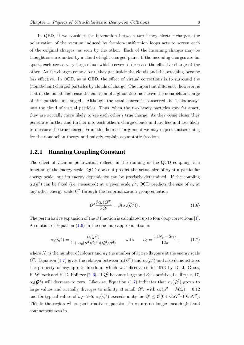
Chapter 1. Physics of Ultra-Relativistic Heavy-Ion Collisions 16
In recent years, the effect of pre-equilibrium conditions on deconfinement have been stud-ied in more detail; in particular, it now appears conceivable that nuclear collisions lead toa specific form of deconfinement without ever producing a thermalized plasma of quarksand gluons. We shall return to these aspects later and here address first the probesproposed to study the different stages and properties of a thermal medium.
free hadrons
pre-equilibriumquark-gluon plasma
hadronic matter t
z
Figure 5: Expected evolution of a nuclear collision
The initial energy density of the produced medium at the time of thermalization wasestimated by [8]
ϵ =
!dNh
dy
"
y=0
wh
πR2Aτ0
, (4)
where (dNh/dy)y=0 specifies the number of hadrons emitted per unit rapidity at mid-rapidity and wh their average energy. The initial volume is determined in the transversenuclear size (radius RA) and the formation time τ0 ≃ 1 fm of the thermal medium.
The determination of the nature of the hot initial phase required deconfinement signatures.It was argued that in a hot quark-gluon plasma, the J/ψ would melt through colourscreening [11], so that QGP formation should lead to a suppression of J/ψ production innuclear collisions. Similarly, the QGP was expected to result in a higher energy loss for afast passing colour charge than a hadronic medium, so that increased jet quenching [12]should also signal deconfinement.
The temperature of the produced medium, in the confined as well as in the deconfinedphase, was assumed to be observable through the mass spectrum of thermal dileptonsand the momentum spectrum of thermal photons [9, 10]. The observation of thermaldilepton/photon spectra would also indicate that the medium was indeed in thermalequilibrium.
The behaviour of sufficiently short-lived resonances, in particular the dilepton decay ofthe ρ, was considered as a viable tool to study the hadronic medium in its interactingstage and thus provide information on the approach to chiral symmetry restoration [13].
The expansion of the hot medium was thought to be measurable through broadening andazimuthal anisotropies of hadronic transverse momentum spectra (flow) [14]. The size andage of the source at freeze-out was assumed to be obtainable through Hanbury-Brown–Twiss (HBT) interferometry based on two-particle correlations [15]. It was expected that
4
Figure 1.7: Schematic representation of the expected space-time evolution of a ultra-relativistic heavy-ion collision.
information on the chemical and kinetic freeze-out temperature and chemical potential,
radial expansion velocity, hydrodynamical properties of the medium, size parameters as
extracted from two-particle correlations, momentum spectra, event-by-event fluctuations
and correlations of hadron momenta and yields. The study of jets originating from hard
partons and of heavy-flavour hadrons provides insights into the interaction mechanisms
inside the QGP. Photons do not interact strongly, thus they probe the state of the matter
at the time of their production: thermal photons radiated off the quarks which undergo
collisions with other quarks and gluons in a thermal bath can be used to measure the
temperature of the medium.
Heavy-ion collisions are an important part of the physics programme of the LHC,
which started operation at the end of 2009. In particular, the heavy-ion programme
at LHC has the aim of precisely characterizing the QGP parameters at the highest
collision energy. A selection of the results from the first years of ion physics at the LHC
at the centre-of-mass energy of√sNN = 2.76 TeV per nucleon pair, also compared with
previous experiments, is presented in the following paragraphs. The description of the
collision geometry will be given and then some observables which allow to characterize
the properties of the Pb–Pb events will be presented, as well as an example of a hard
probe such as the quarkonium production. The aspects directly related to this thesis
work are treated in Chapter 2.

Chapter 1. Physics of Ultra-Relativistic Heavy-Ion Collisions 17
Glauber Modeling in Nuclear Collisions 8
Projectile B Target A
b zs
s-b
bs
s-b
a) Side View b) Beam-line View
B
A
Figure 3: Schematic representation of the Optical Glauber Model geometry, with
transverse (a) and longitudinal (b) views.
2.3 Optical-limit Approximation
The Glauber Model views the collision of two nuclei in terms of the individual
interactions of the constituent nucleons (see, e.g., Ref. (27)). In the optical limit,
the overall phase shift of the incoming wave is taken as a sum over all possible
two-nucleon (complex) phase shifts, with the imaginary part of the phase shifts
related to the nucleon-nucleon scattering cross section through the optical theo-
rem(28,29). The model assumes that at sufficiently high energies, these nucleons
will carry sufficient momentum that they will be essentially undeflected as the
nuclei pass through each other. It is also assumed that the nucleons move inde-
pendently in the nucleus and that the size of the nucleus is large compared to the
extent of the nucleon-nucleon force. The hypothesis of independent linear tra-
jectories of the constituent nucleons makes it possible to develop simple analytic
expressions for the nucleus-nucleus interaction cross section and for the number
of interacting nucleons and the number of nucleon-nucleon collisions in terms of
the basic nucleon-nucleon cross section.
Consider Fig. 3. Two heavy-ions, “target” A and “projectile” B are shown
colliding at relativistic speeds with impact parameter b (for colliding beam ex-
periments the distinction between the target and projectile nuclei is a matter of
convenience). We focus on the two flux tubes located at a displacement s with
respect to the center of the target nucleus and a distance s − b from the center
of the projectile. During the collision these tubes overlap. The probability per
unit transverse area of a given nucleon being located in the target flux tube is
TA (s) =!ρA(s, zA)dzA, where ρA (s, zA) is the probability per unit volume, nor-
malized to unity, for finding the nucleon at location (s, zA). A similar expression
follows for the projectile nucleon. The product TA (s) TB (s− b) d2s then gives
the joint probability per unit area of nucleons being located in the respective
overlapping target and projectile flux tubes of differential area d2s. Integrating
Figure 1.8: Schematic representation of the optical Glauber model geometry withtransverse and longitudinal views.
1.5.1 Geometry of the Collision
Nuclei are extended objects compared to the scales of interest in high energy physics.
For this reason, the geometry of the collision plays an important role in the study of
nuclear matter effects and QGP formation. In the centre-of-mass frame, the two colliding
nuclei can be seen as two thin disks of transverse size 2RA ' 2A1/3 fm (A is the atomic
mass number), since they are Lorentz contracted along the beam direction by a factor
γ = Ebeam/M (Ebeam is the energy of the accelerated nuclei and M their mass). The
quantities used to characterize the collision geometry are:
• The impact parameter, which is the distance between the centres of the two col-
liding nuclei. The impact parameter characterizes the centrality of the collision: a
central collision is one with small impact parameter in which the two nuclei collide
almost head-on, a peripheral collision is one with large impact parameter.
• The number of participant nucleons, Npart, within the colliding nuclei, which is the
total number of protons and neutrons that undergo at least one inelastic collision.
• The number of binary collisions, Ncoll, is the total number of nucleon–nucleon
collisions.
These quantities can be derived from a probabilistic Glauber model [15]. Two heavy
ions colliding with impact parameter b can be represented as in Figure 1.8. The two
flux tubes located at a displacement s with respect to the centre of the target nucleus
and at a distance s−b from the centre of the projectile, overlap during the collision. If
ρA(s − zA) is the probability per unit volume, normalized to unity, for finding a given
nucleon at (s−zA), the probability per unit transverse area of the nucleon being located
in the target flux tube is TA(s) =∫ρA(s− zA)dzA. The product TA(s)TA(s − b)d2s
then gives the joint probability per unit area of nucleons being located in the respective
overlapping target and projectile flux tubes of differential area d2s. Integrating this

Chapter 1. Physics of Ultra-Relativistic Heavy-Ion Collisions 18
product over all values of s defines the nuclear overlap function TAB(b):
TAB(b) =
∫TA(s)TB(s− b)d2s , (1.13)
where b is the magnitude of the impact parameter vector b. TAB(b) has the unit of
inverse area and can be interpreted as the effective overlap area for which a specific
nucleon in A can interact with a given nucleon in B. The probability of an interaction
occurring is then TAB(b)σNNinel, where σNN
inel is the nucleon–nucleon inelastic cross section.
The probability of having n such interactions between nucleus A (with A nucleons) and
nucleus B (with B nucleons) is given by a binomial distribution
P (n, b) =
(AB
n
)[TAB(b)σNN
inel
]n [1− TAB(b)σNN
inel
]AB−n, (1.14)
where the first term is the number of combinations for finding n collisions out of A · Bpossible nucleon–nucleon interactions, the second term is the probability for having
exactly n collisions, and the last term is the probability of exactly A·B−n misses. Based
on this probability distribution, the relevant quantities that characterize the collision
geometry can be determined. The number of nucleon–nucleon collisions4 is
Ncoll(b) =
AB∑
n=1
nP (n, b) = ABTAB(b)σNNinel . (1.15)
The number of participants at impact parameter b is given by
Npart(b) = A
∫TA(s)
{1−
[1− TB(s− b)σNN
inel
]B }d2s+ (1.16)
+ B
∫TB(s− b)
{1−
[1− TA(s)σNN
inel
]A }d2s ,
where the integral over the bracketed terms give the respective inelastic cross sections
for nucleus–nucleus collisions. This formulation of the Glauber model (optical limit) is
based on continuous nucleon density distributions: each nucleon in the projectile sees
the oncoming target as a smooth density.
Neither impact parameter nor Npart or Ncoll are directly measured experimentally.
Mean values of such quantities can be extracted for classes of measured events via a
mapping procedure. Typically, a measured distribution is mapped to the corresponding
distribution obtained from phenomenological analytic or Monte Carlo Glauber calcula-
tions. This is done by defining centrality classes in both the measured and calculated
distributions and then connecting the mean values from the same centrality class in the
two distributions (Figure 1.9).
4Alternatively the number of nucleon–nucleon collisions is expressed as Ncoll(b) = TAB(b)σNNinel if
ρA(s− zA) is normalized to A. This convention is used, for example, in [16].
Chapter 1. Physics of Ultra-Relativistic Heavy-Ion Collisions 19
Glauber Modeling in Nuclear Collisions 14
3 Relating the Glauber Model to Experimental Data
Unfortunately, neither Npart nor Ncoll can be directly measured in a RHIC exper-
iment. Mean values of such quantities can be extracted for classes of (Nevt) mea-
sured events via a mapping procedure. Typically a measured distribution (e.g.,
dNevt/dNch) is mapped to the corresponding distribution obtained from phe-
nomenological Glauber calculations. This is done by defining “centrality classes”
in both the measured and calculated distributions and then connecting the mean
values from the same centrality class in the two distributions. The specifics of this
mapping procedure differ both between experiments as well as between collision
systems within a given experiment. Herein we briefly summarize the principles
and various implementations of centrality definition.
3.1 Methodology
Figure 8: A cartoon example of the correlation of the final state observable
Nch with Glauber calculated quantities (b, Npart). The plotted distribution and
various values are illustrative and not actual measurements (T. Ullrich, private
communication).
The basic assumption underlying centrality classes is that the impact param-
eter b is monotonically related to particle multiplicity, both at mid and forward
rapidity. For large b events (“peripheral”) we expect low multiplicity at mid-
rapidity, and a large number of spectator nucleons at beam rapidity, whereas
for small b events (“central”) we expect large multiplicity at mid-rapidity and a
small number of spectator nucleons at beam rapidity (Figure 8). In the simplest
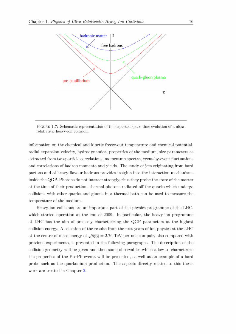
Figure 1.9: Illustration of the correlation between the final state observable Nch andGlauber calculated quantities (b, Npart).
Two experimental observables related to the collision geometry are the charged-
particle multiplicity Nch and the energy carried by particles close to the beam direction
and deposited in the forward zero-degree calorimeters, called the zero-degree energy
EZDC. EZDC is directly related to the number of spectator nucleons, which constitute
the part of the nuclear volume not involved in the interaction.
Particle multiplicity is monotonically related to the impact parameter b. One possi-
bility to define centrality classes is to measure the charged-particle multiplicity distribu-
tion (dσ/dNch). Knowing the total integral of the distribution, one can define centrality
classes by binning the distribution based upon the fraction of the total integral. The
centrality classes are obtained defining shape cuts on the distribution, which correspond
to well defined percentile intervals of the hadronic cross section σtot (0–5%, 5–10%, etc.).
The same procedure is then applied to a calculated distribution and for each centrality
class, the mean value of Glauber quantities, e.g. 〈Npart〉 and 〈Ncoll〉, is extracted.

Chapter 1. Physics of Ultra-Relativistic Heavy-Ion Collisions 20
(GeV)NNs210 310
)⟩p
art
N⟨)/
(0.5
η/d
chN
(d
0
2
4
6
8
10pp NSD ALICEpp NSD CMS
NSD CDFpp NSD UA5pp NSD UA1pp
pp NSD STAR
PbPb(05 %) ALICEPbPb(05 %) NA50AuAu(05 %) BRAHMSAuAu(05 %) PHENIXAuAu(05 %) STARAuAu(06 %) PHOBOS
0.11NN
s ∝
0.15NN
s ∝
AA
)ppp(pMultiplicities
Figure 1.10: Charged-particle pseudorapidity density per participant pair for cen-tral A–A and non-single diffractive pp (pp) collisions as a function of
√sNN. The
solid lines ∝ s0.15NN and ∝ s0.11
NN are superimposed on the heavy-ion and pp (pp) data,respectively [17].
1.5.2 Global Event Properties
Global event properties describe the state and dynamical evolution of the bulk matter
created in a heavy-ion collision by measuring characteristics of the soft particles (with
momentum below few GeV/c), which represent the large majority of produced particles.
They include multiplicity distributions, which can be related to the initial energy density
reached in the collision, yields and momentum spectra of identified particles, which are
determined by the conditions at and shortly after hadronization, and correlation between
particles, which measure both size and lifetime of the dense matter state.
1.5.2.1 Particle Multiplicity
The first step in characterizing the system produced in heavy-ion collisions is the mea-
surement of the number of charged particles produced per unit of pseudorapidity5
(dNch/dη). This can be related to the initial energy density using the formula pro-
posed by Bjorken [18]:
ε =dET/dη
τ0πR2A
=3
2〈ET/N〉
dNch/dη
τ0πR2A
, (1.17)
5The pseudorapidity is defined as η = − ln[tan(θ/2)], where θ is the polar angle with respect to thebeam direction. For a particle with velocity v → c, η ≈ y, being y the longitudinal rapidity. The
longitudinal rapidity of a particle with four-momentum (E, ~p) is defined as y = 12
ln(
E+pzE−pz
), being z
the direction of the beam.

Chapter 1. Physics of Ultra-Relativistic Heavy-Ion Collisions 21
where τ0 denotes the thermalization time, RA is the nuclear radius and ET/N ∼ 1 GeV
is the transverse energy per emitted particle, and the factor 3/2 derives from the as-
sumption that particle multiplicity is dominated by pions (π+, π−, π0) and dNch/dη
measures only the charged pions π±.
In order to compare the bulk particle production in different collision systems and at
different energies, the charged-particle density is scaled by the number of participating
nucleons in the collision (Npart). The charged particle pseudorapidity density normal-
ized per participant pair, dNch/dη/(0.5〈Npart〉) measured by ALICE in central Pb–Pb
collisions at√sNN = 2.76 TeV is shown in Figure 1.10, compared to the lower-energy
measurements for Au–Au and Pb–Pb, and non-single diffractive (NSD) pp and pp col-
lisions over a wide range of collision energies. The energy dependence is steeper for
heavy-ion collisions than for pp and pp collisions. Particle production follows a power
law ∝ s0.15NN in heavy-ion collisions and ∝ s0.11
NN in pp and pp collisions.
The charged-particle pseudorapidity density measured in central collisions at LHC is
dNch/dη ≈ 1600 [17]. This value implies that the initial energy density (at τ0 = 1 fm/c)
is about 15 GeV/fm3 [19] (� εc, the critical energy density), approximately a factor of
three higher than in Au–Au collisions at the top energy of RHIC.
1.5.2.2 Identical Boson Correlations
The freeze-out volume (the size of the matter at the time when strong interactions
cease) and the total lifetime of the created system (the time between collision and
freeze-out) can be studied using identical boson interferometry (also called Hanbury-
Brown-Twiss or HBT) [20]. This technique exploits the Bose-Einstein enhancement of
identical bosons emitted close-by in the phase space, which leads to a modification of
the two-particle correlation function measured in energy and momentum variables. The
space and time distribution of the emitting source, i.e. the space-time hyper surface
of last rescattering, can be inferred via a Fourier transformation. Results from HBT
correlation measurements are shown in Figure 1.11 for central collisions from very low
energies up to LHC as a function of the charged-particle density [21]. Compared to top
RHIC energy, the locally comoving freeze-out volume (Figure 1.11(a)) increases by a
factor two (to about 5000 fm3) and the system lifetime (Figure 1.11(b)) increases by
about 30% (to 10 fm/c). These results contribute to indicate that the fireball formed in
nuclear collisions at the LHC lives longer and expands to a larger size at freeze-out as
compared to lower energies.

Chapter 1. Physics of Ultra-Relativistic Heavy-Ion Collisions 22
⟩ η/dch
dN⟨
0 500 1000 1500 2000
)3 (
fmlo
ngR
side
Rou
t R
3/2
)π
(2
0
1000
2000
3000
4000
5000
6000Phys. Lett. B 696 (2011) 328 (values scaled)
E895 2.7, 3.3, 3.8, 4.3 GeVNA49 8.7, 12.5, 17.3 GeVCERES 17.3 GeVSTAR 62.4, 200 GeVPHOBOS 62.4, 200 GeVALICE 2760 GeV
E895 2.7, 3.3, 3.8, 4.3 GeVNA49 8.7, 12.5, 17.3 GeVCERES 17.3 GeVSTAR 62.4, 200 GeVPHOBOS 62.4, 200 GeVALICE 2760 GeV
(a)
1/3⟩ η/d
chdN⟨
0 2 4 6 8 10 12 14
(fm
/c)
fτ
0
2
4
6
8
10
12
Phys. Lett. B 696 (2011) 328
E895 2.7, 3.3, 3.8, 4.3 GeVNA49 8.7, 12.5, 17.3 GeVCERES 17.3 GeVSTAR 62.4, 200 GeVPHOBOS 62.4, 200 GeVALICE 2760 GeV
E895 2.7, 3.3, 3.8, 4.3 GeVNA49 8.7, 12.5, 17.3 GeVCERES 17.3 GeVSTAR 62.4, 200 GeVPHOBOS 62.4, 200 GeVALICE 2760 GeV
(b)
Figure 1.11: (a) Product of the three pion HBT radii measured by ALICE in redcompared to those obtained for central gold and lead collisions at lower energies atthe AGS, SPS and RHIC. (b) The system lifetime (decoupling time) τf measured byALICE (red filled dot) compared to results from lower energies [21].
1.5.3 Photon Spectrum
One of the signals expected for the QGP is the radiation of “thermal photons”, with
a spectrum reflecting the temperature of the system. These photons come from sec-
ondary interactions among medium constituents and leave the reaction zone created
in a nucleus–nucleus collision without interacting, since their mean-free path is much
larger than nuclear scales. Therefore, they provide a direct probe to examine the early
hot phase of the collision. Thermal photons are produced during the entire evolution
of the QGP and also after the transition to a hot gas of hadrons. The experimental
challenge in detecting them comes from the huge background of photons from hadron
decays (predominantly neutral pions and η mesons). At the LHC, ALICE measured
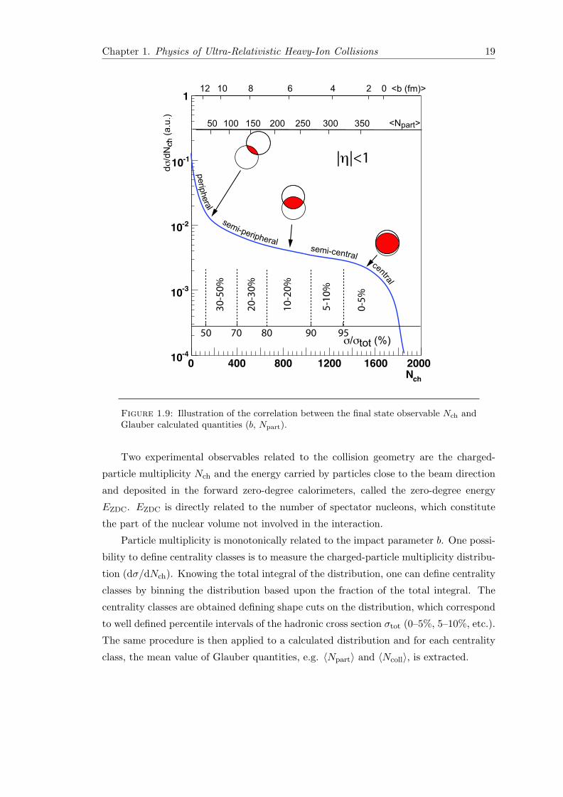
the spectrum of direct photons in central Pb–Pb collision at√sNN = 2.76 TeV, de-
fined as the photons not coming from hadron decays but from initial hard primary
QCD interactions among partons. An excess of photons of about 15% was observed for
1 < pT < 5 GeV/c, with respect to the expectation for hard scattering (Figure 1.12).
In this region, the spectrum has an exponential shape and the inverse slope parameter,
T = 304± 51 (stat.+ syst.) MeV, is larger than the value observed in Au–Au collisions
at RHIC at√sNN = 0.2 TeV, T = 221±19 (stat.)±19 (syst.) MeV [22]. This parameter
can be interpreted as an effective temperature averaged over the time evolution of the
hot system.
1.5.4 Hard Processes
Hard processes, involving high momentum or high mass scales, have much larger cross
sections at LHC with respect to RHIC, due to the increased energy of heavy-ion col-
lisions. Energetic quarks or gluons can be observed as jets or single particles with pT
Chapter 1. Physics of Ultra-Relativistic Heavy-Ion Collisions 23
(GeV/c)T
p0 2 4 6 8 10 12 14
)2 c2
(G
eVdy
Tdp
TpN2 d
ev
. N
π21
710
610
510
410
310
210
110
1
10
210
310
= 2.76 TeVNNs040% PbPb,
Direct photons (scaled pp)
T = 0.5,1.0,2.0 pµDirect photon NLO for
51 MeV±/T), T = 304 T
exp(p×Exponential fit: A
ALI−PREL−27968
Figure 1.12: ALICE preliminary direct photons pT spectrum measured in Pb–Pbcollisions at
√sNN = 2.76 TeV for 40% most central collisions compared at low pT
with an exponential fit and with a direct-photon NLO calculation for pp collisions at√s = 2.76 TeV scaled by the number of nucleon–nucleon binary collisions.
reaching 100 GeV/c and beyond. Similarly, high pT photons, charmonium and bot-
tomonium states and even the weak vector bosons W and Z are copiously produced.
The details of the production and propagation of these high pT probes can be used to
explore the mechanisms of parton energy loss and deconfinement in the medium. The
description of the parton energy loss process in a hot medium will be given in Chapter 2.
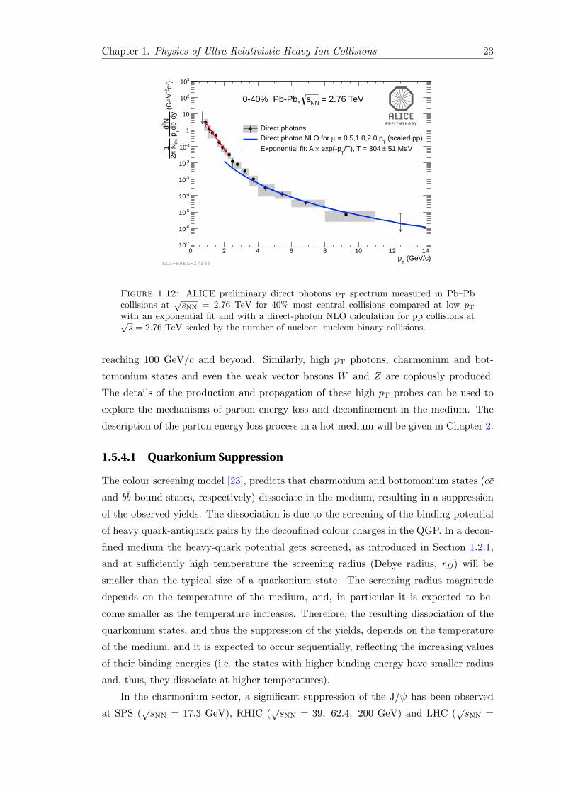
1.5.4.1 Quarkonium Suppression
The colour screening model [23], predicts that charmonium and bottomonium states (cc
and bb bound states, respectively) dissociate in the medium, resulting in a suppression
of the observed yields. The dissociation is due to the screening of the binding potential
of heavy quark-antiquark pairs by the deconfined colour charges in the QGP. In a decon-
fined medium the heavy-quark potential gets screened, as introduced in Section 1.2.1,
and at sufficiently high temperature the screening radius (Debye radius, rD) will be
smaller than the typical size of a quarkonium state. The screening radius magnitude
depends on the temperature of the medium, and, in particular it is expected to be-
come smaller as the temperature increases. Therefore, the resulting dissociation of the
quarkonium states, and thus the suppression of the yields, depends on the temperature
of the medium, and it is expected to occur sequentially, reflecting the increasing values
of their binding energies (i.e. the states with higher binding energy have smaller radius
and, thus, they dissociate at higher temperatures).
In the charmonium sector, a significant suppression of the J/ψ has been observed
at SPS (√sNN = 17.3 GeV), RHIC (
√sNN = 39, 62.4, 200 GeV) and LHC (
√sNN =

Chapter 1. Physics of Ultra-Relativistic Heavy-Ion Collisions 24
2.76 TeV) energies. The results obtained at LHC by ALICE [24] and CMS [25] at forward
rapidity are reported in Figure 1.13(a). At forward rapidity the J/ψ RAA, defined as
the ratio of the pT distribution measured in Pb–Pb collisions to that measured in pp
collisions scaled by the average number of nucleon–nucleon collisions, exhibits a strong
pT dependence and decreases by a factor of 2 from low pT to high pT. This behaviour
strongly differs from that measured by PHENIX at RHIC top energy, which exhibits a
strong suppression also at low pT. A qualitative description of the results can be obtained
assuming that, in addition to the dissociation by colour screening, a regeneration process
takes place in the case of high-energy collisions. At√sNN = 2.76 TeV, the charm quark
yield in the collisions increases with respect to SPS and RHIC energies, because of
the large increase of the cc cross-section towards LHC energy. This may result in the
enhancement of the probability to create J/ψ mesons from recombination of initially
uncorrelated charm quarks. The recombination mechanism is expected to lead to an
increase of the RAA at the LHC with respect to the one observed at RHIC. Furthermore,
in order to recombine, two charm quarks need to be close enough in phase space, so that
low transverse momentum J/ψ production is expected to be favoured.
With the high collision energies and luminosities recently available at RHIC and
LHC, it has been also possible to study bottomonium production in heavy-ion colli-
sions. Compared with the J/ψ case, the probability for the Υ states to be regenerated
in the medium is much smaller due to the lower production cross section of bb pairs.
However, the feed-down contributions from higher-mass resonances into the observed
quarkonium yields, as well as several competing nuclear and medium effects have to
be taken into account. The CMS Collaboration measured the midrapidity production
of bottomonium states in Pb–Pb collisions at√sNN = 2.76 TeV. The Υ(1S) yield is
suppressed by approximately a factor of two with respect to the expectation from pp
collisions and scaling of the hard process yield with the number of binary nucleon–
nucleon collisions. Moreover, the suppression of Υ(2S) is stronger than that of Υ(1S),
as shown in Figure 1.13(b), and the Υ(3S) is almost completely suppressed [26]. The
measurement of the inclusive Υ(1S) production at forward rapidity and down to zero
transverse momentum was carried out by ALICE [27]. The observed suppression of in-
clusive Υ(1S) results stronger in central than in semi-peripheral collisions and shows a
pronounced rapidity dependence over the large domain covered by ALICE (2.5 < y < 4)
and CMS (|y| < 2.4). The data support the hypothesis of increased suppression of less
strongly bound states, but a precise measurement of the feed-down contribution to the
Υ(1S) state and an accurate estimate of the cold nuclear matter effects is required to
make a stringent comparison with models.

Chapter 1. Physics of Ultra-Relativistic Heavy-Ion Collisions 25
)c (GeV/T
p0 1 2 3 4 5 6 7 8 9 10
AA
R
0
0.2
0.4
0.6
0.8
1
1.2
1.4 = 2.76 TeVNNsPbPb
8%±90% global syst. = <4, centrality 0%y, 2.5<µ+µ → ψALICE J/
8.3%±100% global syst. = |<2.4, centrality 0%y, 1.6<|µ+µ → ψCMS J/
ALI−PUB−64806
(a)
]2) [GeV/c-µ+µMass(
7 8 9 10 11 12 13 14
)2E
vent
s / (
0.1
GeV
/c
0
100
200
300
400
500
600
700
800
= 2.76 TeVNNsCMS PbPb
Cent. 0-100%, |y| < 2.4-1bµ = 150 intL
> 4 GeV/cµ
Tp
data
PbPb fit
pp shape
(b)
Figure 1.13: (a) Transverse momentum dependence of the centrality integrated nu-clear modification factor of the J/ψ pT distribution in Pb–Pb at
√sNN = 2.76 TeV
with respect to pp collisions. ALICE result refer to the rapidity range 2.5 < y < 4 [24],CMS one to 1.6 < y < 2.4 [25]. (b) Dimuon invariant mass distribution from Pb–Pbdata at
√sNN = 2.76 TeV. The red line shows the fit to Pb–Pb data. The blue dashed
line shows the shape obtained from the fit to pp data. For a better comparison, thebackground shape, background yield, mass peak width, mass peak tail shape and theΥ(1S) yields in the blue line are fixed to the Pb–Pb fit, while the Υ(2S)/Υ(1S) andΥ(3S)/Υ(1S) ratios are fixed to the pp fit values [26].


2Heavy-Flavour Probes in Heavy-Ion
Collisions
Heavy quarks (charm and beauty) provide sensitive probes of the heavy-ion collision
dynamics at both short and long timescales. On one hand, heavy-flavour production is
an intrinsically perturbative phenomenon which involves large momentum transfer due
to the large mass of the quarks (mc ' 1.5 GeV/c2 and mb ' 5 GeV/c2) and, thus, takes
place on a short timescale, smaller than the formation time of the QGP. On the other
hand, the long lifetime of charm and beauty quarks allows them to live through the
thermalization phase of the plasma and to possibly interact with the constituents of the
medium.
The measurement of charm and beauty production in proton–proton and proton–
nucleus collisions provides the necessary baseline for the study of medium effects in
nucleus–nucleus collisions, and it is of great interest per se, as a test of both pertur-
bative and non-perturbative sectors of QCD. Moreover, proton–nucleus collisions allow
to investigate the cold nuclear matter effects, which are present also in nucleus–nucleus
collisions and need to be disentangled from final state effects in order to understand the
heavy-flavour interaction mechanisms with the medium.
In this chapter, after a brief introduction on the heavy-flavour production in proton–
proton collisions in Section 2.1, the interaction mechanisms of heavy quarks and the
relation to the medium properties will be discussed in Section 2.2 and Section 2.3.
Finally, in Section 2.4, the cold nuclear matter effects, which can be investigated in
proton–nucleus collisions, are described.
27

Chapter 2. Heavy-Flavour Probes in Heavy-Ion Collisions 28
2.1 Heavy-Flavour Production in pp Collisions
Charm and beauty quarks are produced in parton scattering processes involving large
momentum transfers (large virtuality). In these conditions, asymptotic freedom allows to
perform perturbative calculations in terms of αs(Q2), whereQ2 is the scale of the process,
of the order of the energy of the produced particles. Heavy-flavour hadron production
in proton–proton collisions is described, following the collinear factorization approach,
as a convolution of three terms: the parton distribution functions, the hard partonic
scattering cross section and the fragmentation function. The inclusive differential cross
section for the production of a heavy-flavour hadron HQ can be expressed as:
dσpp→HQX(√s,mQ, µ
2F, µ
2R) =
∑
i,j=q,q,g
fi(x1, µ2F) ⊗ fj(x2, µ
2F) ⊗
⊗ dσij→Q(Q){k}(αs(µ2R), µ2
F,mQ, x1x2s) ⊗⊗ D
HQ
Q (z, µ2F) . (2.1)
The partonic cross section dσij→Q(Q){k} is calculated as a perturbative series in the
strong coupling αs, which depends on the energy scale of the process, indicated here as
renormalization scale, µR; currently, calculations are performed up to next-to-leading
order (NLO), O(α3s ) (MNR [28], GM-VFNS [29–31], MC@NLO [32, 33]), or at fixed
order with next-to-leading-log resummation (FONLL [34–36]). The Parton Distribu-
tion Function (PDF), fi(x1, µ2F) encodes the partonic structure of the colliding protons
and can be interpreted as the probability to find a parton i inside the proton with
fraction of momentum x1 = pi/pp (Bjorken x). The fragmentation function DHQ
Q (z, µ2F)
parametrizes the probability for the heavy quark Q to fragment into a hadron HQ with a
momentum fraction z = pHQ/pQ. The PDFs and the fragmentation functions depend on
the energy scale of the process, in particular they evolve as a function of the momentum
transfer Q2. In the cross section calculations they are evaluated at a given scale called
factorization scale µF. The renormalization and factorization scales are usually taken of
the same order of the momentum transfer of the hard process µR ∼ µF ∼√m2Q + p2
T,Q .
The measurement of charm and beauty production at different centre-of-mass en-
ergies provides an interesting test of perturbative QCD (pQCD). Moreover, at LHC
energies, the measurement of charm production in the low transverse momentum region
probes the parton distribution functions of the proton at small values of parton fractional
momentum x (∼ 10−4) and squared momentum transfer Q2. Since at LHC energies
heavy quarks are mainly produced through gluon-gluon fusion processes (gg → QQ),
charm production in pp collisions, in particular, could probe the gluon enhancement, ex-
pected in the low-x regime, arising from non-linear evolution of the parton densities [37].
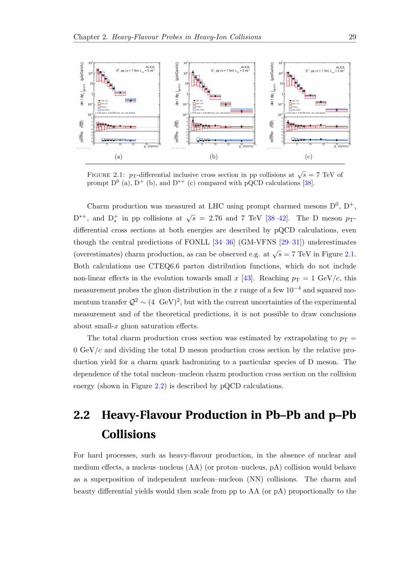
Chapter 2. Heavy-Flavour Probes in Heavy-Ion Collisions 29
GeV/c t
p0 5 10 15 20 25
b/G
eV/c
)µ
(
|y|<
0.5
| t /
dpσd
210
110
1
10
210
310ALICE
1 = 5 nbint
= 7 TeV, Ls, pp 0D
1.3% BR norm. unc. (not shown)± 3.5% lumi, ±
stat. unc.
syst. unc.
FONLL
GMVFNS
(GeV/c)t
p0 5 10 15 20 25
FO
NLL
Dat
a
00.5
11.5
22.5
33.5
(GeV/c) t
p0 5 10 15 20 25
GM
VF
NS
Dat
a
00.5
11.5
22.5
33.5
ALI−PUB−12503
(a)
GeV/c t
p0 5 10 15 20 25
b/G
eV/c
)µ
(
|y|<
0.5
| t /
dpσd
210
110
1
10
210
310ALICE
1 = 5 nbint
= 7 TeV, Ls, pp +D
2.1% BR norm. unc. (not shown)± 3.5% lumi, ±
stat. unc.
syst. unc.
FONLL
GMVFNS
(GeV/c)t
p0 5 10 15 20 25
FO
NLL
Dat
a
00.5
11.5
22.5
33.5
(GeV/c) t
p0 5 10 15 20 25
GM
VF
NS
Dat
a
00.5
11.5
22.5
33.5
ALI−PUB−12507
(b)
GeV/c t
p0 5 10 15 20 25
b/G
eV/c
)µ
(
|y|<
0.5
| t /
dpσd
210
110
1
10
210
310ALICE
1 = 5 nbint
= 7 TeV, Ls, pp *+D
1.5% BR norm. unc. (not shown)± 3.5% lumi, ±
stat. unc.
syst. unc.
FONLL
GMVFNS
(GeV/c)t
p0 5 10 15 20 25
FO
NLL
Dat
a
00.5
11.5
22.5
33.5
(GeV/c) t
p0 5 10 15 20 25
GM
VF
NS
Dat
a
00.5
11.5
22.5
33.5
ALI−PUB−12511
(c)
Figure 2.1: pT-differential inclusive cross section in pp collisions at√s = 7 TeV of
prompt D0 (a), D+ (b), and D∗+ (c) compared with pQCD calculations [38].
Charm production was measured at LHC using prompt charmed mesons D0, D+,
D∗+, and D+s in pp collisions at
√s = 2.76 and 7 TeV [38–42]. The D meson pT-
differential cross sections at both energies are described by pQCD calculations, even
though the central predictions of FONLL [34–36] (GM-VFNS [29–31]) underestimates
(overestimates) charm production, as can be observed e.g. at√s = 7 TeV in Figure 2.1.
Both calculations use CTEQ6.6 parton distribution functions, which do not include
non-linear effects in the evolution towards small x [43]. Reaching pT = 1 GeV/c, this
measurement probes the gluon distribution in the x range of a few 10−4 and squared mo-
mentum transfer Q2 ∼ (4 GeV)2, but with the current uncertainties of the experimental
measurement and of the theoretical predictions, it is not possible to draw conclusions
about small-x gluon saturation effects.
The total charm production cross section was estimated by extrapolating to pT =
0 GeV/c and dividing the total D meson production cross section by the relative pro-
duction yield for a charm quark hadronizing to a particular species of D meson. The
dependence of the total nucleon–nucleon charm production cross section on the collision
energy (shown in Figure 2.2) is described by pQCD calculations.
2.2 Heavy-Flavour Production in Pb–Pb and p–Pb
Collisions
For hard processes, such as heavy-flavour production, in the absence of nuclear and
medium effects, a nucleus–nucleus (AA) (or proton–nucleus, pA) collision would behave
as a superposition of independent nucleon–nucleon (NN) collisions. The charm and
beauty differential yields would then scale from pp to AA (or pA) proportionally to the
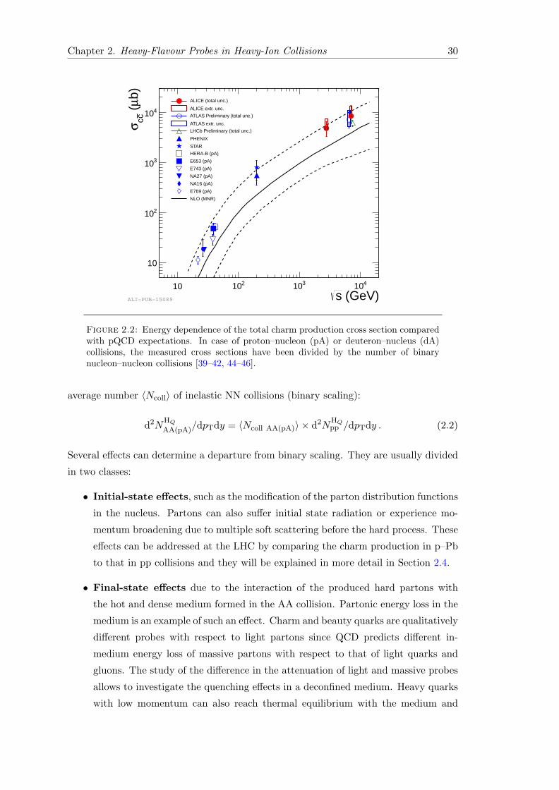
Chapter 2. Heavy-Flavour Probes in Heavy-Ion Collisions 30
(GeV)s10 210 310 410
b)µ
( ccσ
10
210
310
410
ALICE (total unc.)
ALICE extr. unc.
ATLAS Preliminary (total unc.)
ATLAS extr. unc.
LHCb Preliminary (total unc.)
PHENIX
STAR
HERAB (pA)
E653 (pA)
E743 (pA)
NA27 (pA)
NA16 (pA)
E769 (pA)
NLO (MNR)
ALI−PUB−15089
Figure 2.2: Energy dependence of the total charm production cross section comparedwith pQCD expectations. In case of proton–nucleon (pA) or deuteron–nucleus (dA)collisions, the measured cross sections have been divided by the number of binarynucleon–nucleon collisions [39–42, 44–46].
average number 〈Ncoll〉 of inelastic NN collisions (binary scaling):
d2NHQ
AA(pA)/dpTdy = 〈Ncoll AA(pA)〉 × d2NHQpp /dpTdy . (2.2)
Several effects can determine a departure from binary scaling. They are usually divided
in two classes:
• Initial-state effects, such as the modification of the parton distribution functions
in the nucleus. Partons can also suffer initial state radiation or experience mo-
mentum broadening due to multiple soft scattering before the hard process. These
effects can be addressed at the LHC by comparing the charm production in p–Pb
to that in pp collisions and they will be explained in more detail in Section 2.4.
• Final-state effects due to the interaction of the produced hard partons with
the hot and dense medium formed in the AA collision. Partonic energy loss in the
medium is an example of such an effect. Charm and beauty quarks are qualitatively
different probes with respect to light partons since QCD predicts different in-
medium energy loss of massive partons with respect to that of light quarks and
gluons. The study of the difference in the attenuation of light and massive probes
allows to investigate the quenching effects in a deconfined medium. Heavy quarks
with low momentum can also reach thermal equilibrium with the medium and
Chapter 2. Heavy-Flavour Probes in Heavy-Ion Collisions 31
participate in the collective expansion of the system. These effects will be treated
in detail in the next section (Section 2.3).
2.3 Heavy Quarks as QGP Probes
Heavy quarks are produced in the early stage of the Pb–Pb collisions at the LHC on a
temporal and spatial scale proportional to the inverse of the large virtuality Q of the
process, ∆τ ∼ ∆r ∼ 1/Q, thus, sufficiently small for the production to be unaffected
by the properties of the QGP that is formed in the collision. In fact, the minimum
virtuality Qmin = 2mQ in the production of a QQ pair implies a space-time scale of
∼ 1/(2mQ) ' 1/2.4 GeV−1 ' 0.1 fm (for charm), to be compared with the formation
time τ0 ' 1 fm and the lifetime (' 10 fm) of the thermalized QGP. Thus, heavy
quarks experience the full evolution of the system and can be studied to investigate the
properties of the medium. In particular, they are expected to lose energy interacting
with the constituents of the medium, while their multiplicity is not expected to change.
The energy lost by a particle in the medium (∆E) depends on the characteristics of
the particle traversing it (energy, mass and colour charge) and provides fundamental
information on the plasma properties, like the gluon density, particle–medium interaction
coupling, temperature and thickness.
Low-momentum heavy quarks could also participate, through interactions with the
medium, in the collective expansion of the system and eventually reach thermal equilib-
rium with the medium constituents.
Through the measurement of charm and beauty meson production at low and high
momentum, it is also possible to investigate whether the hadronization mechanisms take
place in the medium or via fragmentation in the vacuum, respectively. Hadronization
via recombination in the medium would occur if a quark and an antiquark (or three
quarks) close by in the phase space, thus with similar velocities (direction and magni-
tude), combine together to form a meson (or a baryon). In this case the momentum of
the hadron is equal to the sum of the momenta of the original quarks [47]. Instead, in
case of hadronization via fragmentation of a high-momentum parton in the vacuum, the
hadron carries a fraction of the original momentum of the parton. A possible hadroniza-
tion via recombination of the charm quark with the partons in the medium would affect
the D+s meson production: the medium created in heavy-ion collisions presents an en-
hanced multiplicity of strange quarks [48], and if c quarks recombine in the medium, an
enhancement of D+s /D with respect to pp collisions is expected [49, 50]. Recombination
can also be responsible of an enhanced charmed baryon (e.g. Λ+c ) production relative to
D mesons.
Chapter 2. Heavy-Flavour Probes in Heavy-Ion Collisions 32
2.3.1 In-Medium Energy Loss
The interactions of particles inside a medium are characterized by the following, closely
related, variables:
– mean free path λ = 1/(ρσ) related to the medium density ρ and to the cross section
of the particle-medium interaction σ;
– opacity N = L/λ or number of scatterings experienced by the particle in a medium
of thickness L;
– Debye mass mD is the inverse of the screening length of the colour fields in the
plasma. It is related to the temperature of the medium (mD(T ) ∼ gT , with g equal
to the coupling parameter) and characterizes the typical momentum exchanges
with the medium;
– transport coefficient q, which encodes the scattering power of the medium through
the average transverse momentum squared transferred to the traversing particle
per unit path length. It combines both thermodynamical and dynamical properties
of the medium:
q ≡ m2D
λ= m2
Dρσ =〈k2
T〉λ
; (2.3)
– diffusion constant D which characterizes the dynamics of heavy non-relativistic
particles traversing the plasma.
QCD energy loss differs from QED energy loss mainly because of the non-Abelian
nature of QCD, i.e. the fact that gluons can also interact with each other. The QCD
coupling αs runs faster that αem and the scale Q at which αs(Q) is evaluated needs to
be explicitly considered in all calculations of QCD energy loss. Moreover, it is crucial
to take into account the different coupling of quarks and gluons with the medium. The
relative strengths of the three distinct QCD vertices involved (q → qg, g → gg, and
g → qq) are determined by the structure (Casimir factors) of the gauge SU(3)colour
group. The probability for a gluon to radiate a gluon is proportional to the colour factor
CA = 3, while for a quark the same probability is proportional to CF = 4/3. If the
radiated gluons carry a small fraction of the original parton momentum, the average
number of gluons radiated by a gluon is CA/CF = 9/4 higher than that radiated by a
quark.
Depending on the kinematic region, a colour charge can lose energy1 in a plasma with
temperature T mainly by collisional and radiative mechanisms (Figure 2.3). Therefore,
the total energy loss of a parton traversing a medium is the sum of two terms: ∆E =
∆Ecoll + ∆Erad .
1If the energy of the particle is similar to the plasma temperature, E ∼ O(T ), the particle can alsogain energy while traversing it.

Chapter 2. Heavy-Flavour Probes in Heavy-Ion Collisions 33
4 David d’Enterria
As a numerical QCD example3, let us consider an equilibrated gluon plasmaat T = 0.4 GeV and a strong coupling αs ≈ 0.5 [10]. At this temperature, theparticle (energy) density is ρg = 16/π2 ζ(3) · T 3 ≈ 15 fm−3 (εg = 8π2/15 · T 4
≈ 17 GeV/fm3), i.e. 100 times denser than normal nuclear matter (ρ = 0.15 fm−3).At leading order (LO), the Debye mass is mD = (4παs)
1/2T ≈ 1 GeV. The LOgluon-gluon cross section is σgg ≃ 9πα2
s/(2m2D)≈ 1.5 mb. The gluon mean free
path in such a medium is λg = 1/(ρgσgg)≃ 0.45 fm (the quark mean-free-path isλq =CA/CF λg ≈ 1 fm, where CA/CF = 9/4 is the ratio of gluon-to-quark colourfactors). The transport coefficient is therefore q ≃ m2
D/λg ≃ 2.2 GeV2/fm. Notethat such a numerical value has been obtained with a LO expression in αs forthe parton-medium cross section. Higher-order scatterings (often encoded in a“K-factor” ≈ 2 – 4) could well result in much larger values of q.
• the diffusion constant D, characterising the dynamics of heavy non-relativisticparticles (mass M and speed v) traversing the plasma, is connected, via the Ein-stein relations
D = 2T 2/κ = T/(M ηD) (3)
to the momentum diffusion coefficient κ – the average momentum squared gainedby the particle per unit-time (related to the transport coefficient as κ≈ q v) – andthe momentum drag coefficient ηD.
2.2 Mechanisms of in-medium energy loss
In a general way, the total energy loss of a particle traversing a medium is the sum ofcollisional and radiative terms4: ∆E = ∆Ecoll +∆Erad . Depending on the kinematicregion, a (colour) charge can lose energy5 in a plasma with temperature T mainly bytwo mechanisms6.
E E- E!
!E
E
E- E!
!E
X(medium)
Fig. 3. Diagrams for collisional (left) and radiative (right) energy losses of a quark of energyE traversing a quark-gluon medium.
• Collisional energy loss through elastic scatterings with the medium constituents(Fig. 3, left) dominates at low particle momentum. The average energy loss in
3 For unit conversion, multiply by powers of !c ≃ 0.2 GeV fm (other useful equalities:10 mb = 1 fm2, and 1 GeV−2 = 0.389 mb).
4 In addition, synchrotron-, Cerenkov- and transition-radiation energy losses can take placerespectively if the particle interacts with the medium magnetic field, if its velocity is greaterthan the local phase velocity of light, or if it crosses suddenly from one medium to another.Also, plasma instabilities may lead to energy losses. Yet, those effects – studied e.g. in [11,12, 13, 14] for QCD plasmas – are generally less important in terms of the amount of Eloss.
5 Note that if the energy of the particle is similar to the plasma temperature, E ∼ O(T ), theparticle can also gain energy while traversing it.
6 Note that the separation is not so clear-cut since the diagrams assume well-defined asymp-totic out states, but the outgoing particles may still be in the medium and further rescatter.
Figure 2.3: Diagrams for collisional (left) and radiative (right) energy losses of aquark of energy E traversing a quark-gluon medium.
Collisional energy loss
Collisional energy loss is due to elastic scatterings with the medium constituents (Fig-
ure 2.3, left) and dominates at low particle momentum. The average energy loss in one
scattering (with cross section dσ/dt, where t = Q2 is the squared momentum transfer)
in a medium of temperature T is:
〈∆E1scattcoll 〉 ≈
1
σT
∫ tmax
m2D
tdσ
dtdt , (2.4)
where tmax is the maximum squared momentum transfer, σ the integrated particle-
medium interaction cross section andmD the Debye mass. If one considers the momentum-
transfer integral limits given by the QGP Debye mass squared tmin = m2D(T ) ∼ 4παsT
2(1+
nf/6) and tmax = s ∼ ET and as the dominant contribution to the parton-parton t-
differential elastic cross section
dσ
dt≈ Ci
4πα2s (t)
t2, (2.5)
where Ci = 9/4, 1, 4/9 are the colour factors for gg, gq and qq scatterings respectively, one
obtains for a parton of energy E inside a QGP of temperature T (for E � m2q/T ) [51]:
– Light quark, gluon: − dEcolldl
∣∣∣q,g
= 14CRαs(ET )m2
D ln(ETm2
D
),
– Heavy quark: − dEcolldl
∣∣∣Q
= − dEcolldl
∣∣∣q− 2
9CRπT2
[αs(m
2Q)αs(ET ) ln
(ETm2
Q
)],
with CR = 4/3 (3) being the quark-gluon (gluon-gluon) coupling. −dEdl = 〈∆Etot〉
L is
defined as the energy loss per unit length or stopping power. For incoherent scatterings
one has: ∆Etot = N ·∆E1scatt . The energy loss per unit length reduces to −dE/dl =
〈∆E1scat〉/λ . The amount of ∆Ecoll is linear with the medium thickness and it has a
logarithmic dependence on the initial parton energy.

Chapter 2. Heavy-Flavour Probes in Heavy-Ion Collisions 34
The fact that heavy-quark masses are well above the typical temperature of the
system, mQ � T , allows also a diffusion treatment of their elastic interactions with the
medium which can be parametrized in terms of Brownian motion of a heavy test parti-
cle in a bath of light-particle fluid. Non-relativistically, the typical thermal momentum
transfer of a heavy quark is pth ' 3mQT � T 2, and therefore much larger than the
typical momentum transfer from the medium, Q2 ∼ T 2. This allows to expand the
Boltzmann equation in momentum transfer to arrive at a Fokker-Planck description of
heavy-quark diffusion in the QGP, which directly yields the pertinent transport coeffi-
cients, as will be explained in the following. The transport coefficients are related to
the underlying (elastic) scattering matrix elements on light partons in the QGP which
allow for direct comparisons of microscopic models of the heavy-quark interaction.
The starting point for the derivation of the Fokker-Plank equation is the Boltzmann
equation for the heavy-quark phase-space distribution, fQ,
[∂
∂t+
p
ωp
∂
∂x+ F
∂
∂p
]fQ(t,x,p) = C[fQ] , (2.6)
where ωp =√m2Q + p2 denotes the energy of a heavy quark with 3-momentum p, F is
the mean-field force on the test particle due to an external (in-medium) potential, and
C[fQ] summarizes the collision integral induced by scattering off particles in the heat
bath. Neglecting mean-field effects, and assuming an uniform medium, by integration
over the fireball volume, Equation (2.6) simplifies to an equation for the distribution
function, fQ, of the heavy quark in momentum space determined by the collisions term:
∂
∂tfQ(t,p) = C[fQ] . (2.7)
The collision integral C[fQ] encodes the transition rate for collisions of a heavy quark
with heath-bath particles. The relevant momentum transfers to the heavy quark can
be considered much smaller than the heavy-quark momentum p, and Equation (2.7) is
approximated by the Fokker-Plank equation
∂
∂tfQ(t,p) =
∂
∂pi
{Ai(p)fQ(t,p) +
∂
∂pj[Bij(p)fQ(t,p)]
}. (2.8)
The transport coefficients Ai and Bij depend on the transition rate. Ai encodes the
average momentum change of the heavy quark per unit time and thus describes the
friction in the medium, while Bij represents the average momentum broadening per
unit time, i.e. the diffusion in momentum-space. For an isotropic medium (in thermal
equilibrium) in a non-relativistic regime the transport coefficients can be reduced to
two constants γ and D, further simplifying the Fokker-Plank equation. Solving this
new equation one sees that γ determines the relaxation rate of the average momentum

Chapter 2. Heavy-Flavour Probes in Heavy-Ion Collisions 35
to its equilibrium value, it is a drag or friction coefficient (γ = τ−1therm, where τtherm is
the thermal relaxation time). D is the momentum-diffusion constant, describing the
momentum fluctuations. Moreover, since in thermal equilibrium the heavy quarks have
to obey an equilibrium distribution with the temperature T of the bath, the drag and
diffusion coefficients should satisfy the Einstein dissipation-fluctuation relation,
D = mQγT . (2.9)
The spatial diffusion coefficient, Ds, which describes the broadening of the spa-
tial distribution with time, is related to the drag and momentum-diffusion coefficients
through
Ds =T
mQγ=T 2
D. (2.10)
The heavy-quark friction and diffusion coefficients in the QGP have been calculated
with several microscopic approaches. A perturbative expansion of the elastic scattering
off thermal partons shows poor convergence for coupling constants believed to be relevant
for a QGP as formed in heavy-ion collisions (αs ∼ 0.1). Thus, alternative methods have
been investigated:
– perturbative QCD with running coupling constant at low momentum transfer or
reduced screening mass;
– non-perturbative calculations implementing resonance-like correlations in the QGP
using heavy-quark effective theory, in-medium T -matrices with heavy-quark po-
tentials estimated from thermal lattice QCD;
– evaluations based on the strong-coupling limit of conformal field theory (CFT)
using a conjectured correspondence to string theory in Anti-de-Sitter (AdS) space.
In Figure 2.4 the transport coefficients for charm quark, obtained with the different
approaches mentioned before, are reported as a function of temperature for p = 0. As
can be observed in the left panel (Figure 2.4(a)), close to the critical temperature Tc,
the T−matrix approach, the pQCD calculation with running αs and the AdS/CFT
correspondence matched to QCD are not much different and share overlap around
γ ' 0.2 c/fm. Figure 2.4(b) shows the dimensionless quantity 2πTDs for leading or-
der pQCD, leading order pQCD with running coupling, effective resonance model and
T−matrix approach. The former three are fairly constant as a function of temperature
while T−matrix approach exhibits a significant increase with temperature, indicating
maximal interaction strength close to Tc. This originates from the increasing potential
strength (decrease in colour screening) with decreasing temperature, enhancing reso-
nance correlations at lower temperature.

Chapter 2. Heavy-Flavour Probes in Heavy-Ion Collisions 36
August 1, 2009 6:56 WSPC/INSTRUCTION FILE hq-qgp4
32 R. Rapp, H. van Hees
0
0.1
0.2
0.3
0.4
0.5
0 1 2 3 4 5
γ (1
/fm
)
p (GeV)
1.1 Tc1.4 Tc1.8 Tc
0
0.2
0.4
0.6
0.8
1
0.2 0.25 0.3
γ (1
/fm
)
T (GeV)
pQCD, αs=0.3-0.4reso+pQCDT-matrix+pQCDAdS/CFTpQCD, αs run
Fig. 13. (Color online) Charm-quark friction coefficients, γ, in the QGP. Left panel: three-momentum dependence at three temperatures (color code) for: LO-pQCD with fixed αs = 0.4and µD = gT (dash-dotted lines), heavy-light quark T -matrix plus LO-pQCD for gluons (solidlines)45, and pQCD with running αs and reduced infrared regulator (dashed lines)66,67. Rightpanel: temperature dependence of γ for LO-pQCD, T -matrix plus LO-pQCD (gluons only), pQCDwith running αs, and from AdS/CFT correspondence matched to QCD108 with C = 1.5-2.6115.
non-trivial task, e.g., maintaining gauge invariance); it would be illuminating to ex-
tract a static gluon-exchange (Coulomb) potential for a given set of parameters. The
T -matrix approach performs a resummation of the ladder series of a static (color-
electric) potential; magnetic interactions are implemented in a simplified manner
using the Breit current-current interaction from electrodynamics. It has been veri-
fied that for large center-of-mass energies, the qQ T -matrix recovers the result for
perturbative scattering. However, a number of effects are neglected and need to
be scrutinized, including the interactions with gluons beyond pQCD, retardation,
extra gluon or particle/antiparticle emission (e.g., in a coupled channel treatment)
and the validity (and/or accuracy) of a potential approach at finite temperature
(this issue will reappear in the context of heavy quarkonia in Sec. 4). In the colli-
sional dissociation approach, it would be interesting to explore medium effects in the
employed potential (i.e., on the mesonic wave function). Ideally, by improving on
specific assumptions in a given approach, an agreement would emerge establishing
a common result. Explicit connections with the AdS/CFT results are more difficult
to identify. Maybe it is possible to push the T -matrix approach into a regime of
“large” coupling, or study the existence and properties of (D and B) bound states
in the string theory setting. In Fig. 13 we summarize the drag coefficients as func-
tion of momentum (for three temperatures, left panel) and temperature (for p = 0,
right panel) resulting from the approaches discussed above, i.e.,
(i) leading-order pQCD calculations with fixed αs = 0.4 and Debye-screening mass,
µD = gT , in the t-channel gluon-exchange contributions to the matrix elements
for elastic gQ and qQ scattering,
(ii) in-medium T -matrix calculations using lQCD-based qQ potentials, augmented
by the leading-order pQCD matrix elements for elastic gQ scattering45,
(a)
August 1, 2009 6:56 WSPC/INSTRUCTION FILE hq-qgp4
Heavy quarks in the quark-gluon plasma 33
0
10
20
30
0.2 0.25 0.3 0.35 0.4
2πT
Ds
T (GeV)
charm quarksT-mat+pQCDreso + pQCDpQCDpQCD run. αs
0
10
20
30
0.2 0.25 0.3 0.35 0.4
2πT
Ds
T (GeV)
bottom quarksT-mat + pQCDreso + pQCDpQCDpQCD run. αs
Fig. 14. (Color online) Spatial diffusion coefficient, Ds = T/(γmQ), for c (left) and b quarks (right)in a QGP for: LO-pQCD with fixed αs = 0.4 (dashed lines), effective resonance model + LO-pQCD (bands for ΓD,B = 0.4-0.75 GeV)25, T -matrix approach + LO-pQCD (gluons only)45 and
pQCD with running αs (dash-dotted line)66,67. The AdS/CFT result corresponds to 2πTDs =2π/C ≃ 1.5− 4 (not shown in the plots).
(iii) pQCD calculations with running αs and reduced screening mass66,67, and
(iv) the AdS/CFT correspondence matched to QCD108 with γQCD = CT 2/mQ for
C = 1.5-2.6115 .
At all temperatures, the T -matrix approach, (ii), produces significantly more HQ
interaction strength than LO pQCD, (i), while for T> 0.2GeV the thermaliza-
tion rate for the T -matrix is a factor of ∼2-4 less than for AdS/CFT, (iv), or for
LO-pQCD with running coupling and reduced infrared regulator, (iii). Close to
Tc≃ 180MeV, however, the three approaches (ii), (iii) and (iv) are not much dif-
ferent and share overlap around γ≃ 0.2 c/fm. The spread in the numerical results
reiterates the necessity for systematic checks as indicated above.
Finally, one can convert the drag coefficients into estimates of other HQ trans-
port coefficients of the QGP. Within the Fokker-Planck approach the spatial dif-
fusion coefficient, Ds, is directly related to the drag coefficient, γ, as given by
Eq. (24). Fig. 14 shows the dimensionless quantity 2πTDs for charm (left panel)
and bottom quarks (right panel) as a function of temperature for LO pQCD, LO
pQCD with running coupling and reduced infrared regulator, effective resonance
model and T -matrix approach. The former three are fairly constant as a function
of temperature while the T -matrix approach exhibits a significant increase with
temperature, indicating maximal interaction strength close to Tc. This originates
from the increasing potential strength (decrease in color-screening) with decreasing
temperature, enhancing resonance correlations at lower temperature. It is tempting
to interpret this feature as a precursor phenomenon of hadronization. However, its
robustness needs to be checked with a broader range of lattice potentials. We recall
that the internal-energy based potentials probably provide an upper estimate for
the strength of the interaction. It is interesting to note that for all approaches the
results for b quarks coincide with the ones for c quarks within ∼20-30%. The largest
(b)
Figure 2.4: (a) Charm-quark friction coefficient γ in the QGP as a function of tem-perature for LO-pQCD with fixed αs = 0.4 [52], T−matrix plus LO-pQCD for glu-ons [53], pQCD with running αs [54, 55], and from AdS/CFT correspondence matchedto QCD [56]. (b) Charm spatial diffusion coefficient Ds in the QGP for: LO-pQCDwith fixed αs = 0.4 [52], effective resonance model plus LO-pQCD, T−matrix approachplus LO-pQCD for gluons [53], and pQCD with running αs [54, 55].
Radiative energy loss
The dominant mechanism of energy loss of a fast parton in a QCD environment is of
radiative nature: a parton traversing a QGP loses energy mainly by medium-induced
multiple gluon emission (Figure 2.3, right). This loss can be determined from the cor-
responding single- or double-differential gluon Bremsstrahlung spectrum (ωdIrad/dω or
ωdIrad/d2ωdk2
T, where ω, kT are the energy and transverse momentum of the radiated
gluon, respectively):
〈∆E1scattrad 〉 =
∫ E
ωdIraddω
dω, or 〈∆E1scattrad 〉 =
∫ E ∫ kT,max
ωd2Iraddωdk2
T
dωdk2T . (2.11)
As an example, the general concepts of the BDMPS model [57, 58] are reported
here. An energetic parton produced in a hard collision undergoes, along its path in the
dense medium, multiple scatterings in a Brownian-like motion with mean free path λ,
which decreases as the medium density increases. The medium is modeled with static
scattering centres, which implies that in the multiple scattering process the gluons in the
parton wave function pick up transverse momentum kT with respect to its direction and
they may eventually decohere and be radiated. The scale of the energy loss is set by the
characteristic energy of the radiated gluons, which depends on L and on the properties
of the medium:
ωc = qL2/2 , (2.12)

Chapter 2. Heavy-Flavour Probes in Heavy-Ion Collisions 37
where q is the transport coefficient of the medium. In the case of a static medium, the
distribution of energy ω of the radiated gluons (for ω � ωc) is of the form:
ωdIraddω
' 2αsCRπ
√ωc2ω
. (2.13)
The average energy loss of the parton is thus:
〈∆E1scattrad 〉 =
∫ ωc
0ω
dIraddω
dω ∝ αsCRωc ∝ αsCRqL2 . (2.14)
The average energy loss is: proportional to αsCR and, thus, larger by a factor 9/4 = 2.25
for gluons than for quarks; proportional to the transport coefficient of the medium;
proportional to L2; independent of the initial parton energy E.
For heavy quarks, because of their large mass, the radiative energy loss should
be lower than for light quarks. Heavy quarks with moderate energy, i.e. mQ/E � 0,
propagate with a velocity β =√
1− (mQ/E)2 significantly smaller than the velocity of
light, β = 1. As a consequence, in the vacuum, gluon radiation at angles Θ smaller
than the ratio of their mass to their energy Θ0 = mQ/E is suppressed. The relatively
depopulated cone around the heavy-quark direction with Θ < Θ0 is called the dead
cone. The dead-cone effect is assumed to characterize also in-medium gluon radiation,
and the energy distribution of the radiated gluons, for heavy quarks, is estimated to be
suppressed by a factor
ωdI
dω
∣∣∣∣Heavy
/ωdI
dω
∣∣∣∣Light
=
[1 +
Θ20
Θ2
]−2
=
[1 +
(mQ
E
)2
√ω3
q
]−2
≡ FH/L(mQ/E, q, ω) ,
(2.15)
where the expression for the characteristic gluon emission angle Θ ' (q/ω3)1/4 has
been used. The dead-cone suppression factor FH/L increases (less suppression) as the
heavy-quark energy E increases (the mass becomes negligible) and it decreases at large
ω, indicating that the high-energy part of the gluon radiation spectrum is drastically
suppressed by the dead-cone effect [59].
Due to the aforementioned hierarchy of flavour-dependent collisional and radiative
energy losses, the medium effects are expected to be larger for gluons and light quarks
than for c and b quarks: ∆E(g) > ∆E(q) > ∆E(c) > ∆E(b) (Figure 2.5).
Jet Quenching
Medium-induced parton energy loss in nucleus–nucleus collisions results in various con-
sequences, mostly observed through comparison with proton–proton collisions.
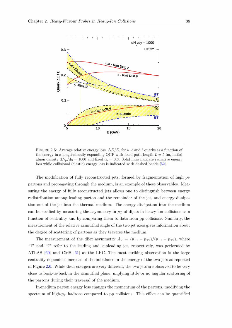
Chapter 2. Heavy-Flavour Probes in Heavy-Ion Collisions 38
August 1, 2009 6:56 WSPC/INSTRUCTION FILE hq-qgp4
36 R. Rapp, H. van Hees
5 10 15 20E (GeV)
0
0.1
0.2
0.3
Qu
ark ∆
E /
E
c - Rad DGLV
c -Elastic
b -Elasticb - Rad DGLV
BT
TG
BT
u,d - Elastic
u,d - Rad DGLV
dNg/dy = 1000
L=5fm
TG
0 2 4 6 8 10 12 14 16 18 20pT (GeV)
0
0.2
0.4
0.6
0.8
1
RQ
(pT)
b
u
c
g
dNg/dy = 1000, L = 5 fm
uc
b
g
DGLV rad + TG elastic
Rad only
Rad + Elastic
Fig. 15. (Color online) Left panel: average relative E-loss, ∆E/E, for u, c and , b quarks as afunction of jet energy, E, in a longitudinally (Bjorken) expanding QGP, with fixed path lengthL = 5 fm, initial gluon rapiditiy density dNg/dy = 1000 and fixed αs = 0.3; the gluon (light-quark)mass is set to µD/
√2 (µD/2), the c(b)-quark mass to mc = 1.2(4.75)GeV (solid lines: radiatve
E-loss, dashed bands: elastic E-loss in two schemes as discussed in the text). Right panel: partonnuclear modification factor, RAA≡RQ, for gluons, u-, c-, and b-quarks as a function of pT for afixed path length and dNg/dy = 1000 (dashed lines: radiative E-loss, solid lines: radiative+elasticE-loss).
is given by
f(v) =1
v2
!v +
1
2(v2 − 1) ln
"1 + v
1− v
#$, (62)
while estimates for Bc are taken from Refs. [Bj]123, [TG]124, and [BT]68,69. The
different values for Bc obtained in these models are considered as reflecting theo-
retical uncertainties. The radiative E-loss within the DGLV reaction-operator ap-
proach is calculated in Ref.122 based on Refs.121,125. The left panel of Fig. 15
compares pQCD radiative and collisional E-loss for various quark flavors (masses)
at high pT > 5GeV in a gluon plasma (GP) with T ≃ 240MeV. For light and
charm (bottom) quarks the elastic E-loss is comparable to the radiative one up
to pT ≃ 10(20)GeV, and still significant above. The right panel of Fig. 15 reiter-
ates that, within pQCD, collisional E-loss is an essential component in calculating
the suppression of light-parton and especially HQ spectra at RHIC. Note that the
relative importance of collisional E-loss is expected to increase if non-perturbative
effects become relevant (which predominantly figure toward lower pT ), or if the GP
is replaced by a QGP.
2.7. D Mesons in the Hadronic Phase
To complete the discussion of open charm in QCDmatter we briefly address medium
modifications of charm hadrons in hadronic matter. Pertinent studies may be di-
Figure 2.5: Average relative energy loss, ∆E/E, for u, c and b quarks as a function ofthe energy in a longitudinally expanding QGP with fixed path length L = 5 fm, initialgluon density dNg/dy = 1000 and fixed αs = 0.3. Solid lines indicate radiative energyloss while collisional (elastic) energy loss is indicated with dashed bands [52].
The modification of fully reconstructed jets, formed by fragmentation of high pT
partons and propagating through the medium, is an example of these observables. Mea-
suring the energy of fully reconstructed jets allows one to distinguish between energy
redistribution among leading parton and the remainder of the jet, and energy dissipa-
tion out of the jet into the thermal medium. The energy dissipation into the medium
can be studied by measuring the asymmetry in pT of dijets in heavy-ion collisions as a
function of centrality and by comparing them to data from pp collisions. Similarly, the
measurement of the relative azimuthal angle of the two jet axes gives information about
the degree of scattering of partons as they traverse the medium.
The measurement of the dijet asymmetry AJ = (pT1 − pT2)/(pT1 + pT2), where
“1” and “2” refer to the leading and subleading jet, respectively, was performed by
ATLAS [60] and CMS [61] at the LHC. The most striking observation is the large
centrality-dependent increase of the imbalance in the energy of the two jets as reported
in Figure 2.6. While their energies are very different, the two jets are observed to be very
close to back-to-back in the azimuthal plane, implying little or no angular scattering of
the partons during their traversal of the medium.
In-medium parton energy loss changes the momentum of the partons, modifying the
spectrum of high-pT hadrons compared to pp collisions. This effect can be quantified

Chapter 2. Heavy-Flavour Probes in Heavy-Ion Collisions 394
JA0 0.2 0.4 0.6 0.8 1
J)
dN/d
Aev
t(1
/N
0
1
2
3
440-100%
JA0 0.2 0.4 0.6 0.8 1
J)
dN/d
Aev
t(1
/N
0
1
2
3
420-40%
JA0 0.2 0.4 0.6 0.8 1
J)
dN/d
Aev
t(1
/N
0
1
2
3
410-20%
JA0 0.2 0.4 0.6 0.8 1
J)
dN/d
Aev
t(1
/N
0
1
2
3
40-10%
ATLASPb+Pb
=2.76 TeVNNs
-1bµ=1.7 intL
φ∆2 2.5 3
φ∆
) dN
/dev
t(1
/N
-210
-110
1
10
φ∆2 2.5 3
φ∆
) dN
/dev
t(1
/N
-210
-110
1
10
φ∆2 2.5 3
φ∆
) dN
/dev
t(1
/N
-210
-110
1
10
φ∆2 2.5 3
φ∆
) dN
/dev
t(1
/N
-210
-110
1
10Pb+Pb Data
p+p Data
HIJING+PYTHIA
FIG. 3: (top) Dijet asymmetry distributions for data (points) and unquenched HIJING with superimposed PYTHIA dijets(solid yellow histograms), as a function of collision centrality (left to right from peripheral to central events). Proton-protondata from
ps = 7 TeV, analyzed with the same jet selection, is shown as open circles. (bottom) Distribution of ��, the
azimuthal angle between the two jets, for data and HIJING+PYTHIA, also as a function of centrality.
(asymmetries larger than 0.6 can only exist for leadingjets substantially above the kinematic threshold of 100GeV transverse energy). The �� distributions show thatthe leading and second jets are primarily back-to-back inall centrality bins; however, a systematic increase is ob-served in the rate of second jets at large angles relativeto the recoil direction as the events become more central.
Numerous studies have been performed to verify thatthe events with large asymmetry are not produced bybackgrounds or detector e↵ects. Detector e↵ects primar-ily include readout errors and local acceptance loss due todead channels and detector cracks. All of the jet eventsin this sample were checked, and no events were flaggedas problematic. The analysis was repeated first requiringboth jets to be within |⌘| < 1 and |⌘| < 2, to see if thereis any e↵ect related to boundaries between the calorime-ter sections, and no change to the distribution was ob-served. Furthermore, the highly-asymmetric dijets werenot found to populate any specific region of the calorime-ter, indicating that no substantial fraction of producedenergy was lost in an ine�cient or uncovered region.
To investigate the e↵ect of the underlying event, thejet radius parameter R was varied from 0.4 to 0.2 and0.6 with the result that the large asymmetry was not re-duced. In fact, the asymmetry increased for the smallerradius, which would not be expected if detector e↵ectsare dominant. The analysis was independently corrobo-rated by a study of “track jets”, reconstructed with IDtracks of pT > 4 GeV using the same jet algorithms. TheID has an estimated e�ciency for reconstructing charged
hadrons above pT > 1 GeV of approximately 80% in themost peripheral events (the same as that found in 7 TeVproton-proton operation) and 70% in the most centralevents, due to the approximately 10% occupancy reachedin the silicon strips. A similar asymmetry e↵ect is alsoobserved with track jets. The jet energy scale and under-lying event subtraction were also validated by correlatingcalorimeter and track-based jet measurements.The missing ET distribution was measured for mini-
mum bias heavy ion events as a function of the total ET
deposited in the calorimeters up to about ⌃ET = 10 TeV.The resolution as a function of total ET shows the samebehavior as in proton-proton collisions. None of theevents in the jet selected sample was found to have ananomalously large missing ET .The events containing high-pT jets were studied for the
presence of high-pT muons that could carry a large frac-tion of the recoil energy. Fewer than 2% of the eventshave a muon with pT > 10 GeV, potentially recoilingagainst the leading jet, so this can not explain the preva-lence of highly asymmetric dijet topologies in more cen-tral events.None of these investigations indicate that the highly-
asymmetric dijet events arise from backgrounds ordetector-related e↵ects.In summary, first results are presented on jet recon-
struction in lead-lead collisions, with the ATLAS detectorat the LHC. In a sample of events with a reconstructedjet with transverse energy of 100 GeV or more, an asym-metry is observed between the transverse energies of the
Figure 2.6: Dijet asymmetry (top) and azimuthal angle between the leading andsubleading jets (bottom) as a function of collision centrality (from peripheral to central)for pp and Pb–Pb collisions [60].
through the nuclear modification factor RAA. This observable is defined as the ratio
of particle production measured in nucleus–nucleus to that expected from the proton–
proton spectrum scaled by the average number of binary nucleon–nucleon collisions
〈Ncoll〉 occurring in the AA collision. Using the nuclear overlap function, defined as
the convolution of the nuclear density profiles of the colliding ions in Section 1.5.1, the
nuclear modification factor of the transverse momentum distribution can be expressed
as:
RAA(pT) =dNAA/dpT
〈TAA〉dσpp/dpT, (2.16)
where the AA spectrum corresponds to a given collision-centrality class and 〈TAA〉 is the
average nuclear overlap function for that centrality class (proportional to 〈Ncoll〉). In-
medium energy loss determines a suppression, RAA < 1, of hadrons at moderate-to-high
transverse momentum. The transport approach for heavy-quark diffusion in the QGP
predicts a reduction of the RAA with an increasing of the interaction strength, thus a
decreasing spatial diffusion coefficient.
The measurement of the D0 meson nuclear modification factor in Au–Au collisions
at√sNN = 200 GeV at RHIC shows no suppression in peripheral collisions, but a
strong suppression, at the level of RAA ∼ 0.5, in the most central collisions for pT >
3 GeV/c [62] (Figure 2.7). This observation suggests a significative energy loss of charm
quarks in the hot medium. The enhancement in the intermediate-pT region is consistent
with model calculations including strong charm–medium interactions and hadronization
via coalescence (recombination with other quarks from the medium) at intermediate pT.
The RAA measurement for charged particles, charged pions and D mesons in the

Chapter 2. Heavy-Flavour Probes in Heavy-Ion Collisions 40
6
0 2 4 60
0.5
1
1.5
2
)A
AF
acto
r (R
40-80% (a)
0 2 4 6 8
10-40% (b)
(GeV/c)T
p0 2 4 6 8
0
0.5
1
1.5
2
Nuc
lear
Mod
ifica
tion
+ X @ 200 GeV Central 0-10%0 D→STAR Au+Au
(c)dataTAMUSUBATECHTorinoDuke w shad.Duke w/o shad.LANL
FIG. 3: (Color online) Panels (a)(b): D0 RAA for peripheral40−80% and semi-central 10−40% collisions; Panel (c): D0
RAA for 0−10% most central events (blue circles) comparedwith model calculations from the TAMU (solid curve), SUB-ATECH (dashed curve), Torino (dot-dashed curve), Duke(long-dashed and long-dot-dashed curves), and LANL groups(filled band). The vertical lines and boxes around the datapoints denote the statistical and systematic uncertainties.The vertical bars around unity denote the overall normaliza-tion uncertainties in the Au+Au and p+p data, respectively.
⟩part
N⟨0 100 200 300 400
AA
R0In
tegr
ated
D
0
0.5
1
1.5
2
p+pnorm.
+ X @ 200 GeV, |y|<10 D→STAR Au+Au
< 8.0 GeV/cT
3.0 < p
< 2.2 GeV/cT
0.7 < p < 8.0 GeV/cT
0 < p
0-80% MB
FIG. 4: (Color online) Integrated D0 RAA as a function ofNpartin different pT regions: 0−8 GeV/c (square), 3−8 GeV/c(circles) and 0.7−2.2 GeV/c (diamonds). Open symbols arefor the 0−80% MB events.
GeV/c [8].The integrated RAA is calculated as the ratio of the
integrated yield in Au+Au collisions divided by the in-tegration of the p+p reference as above scaled by thenumber of binary collisions in the given pT region. Fig-ure 4 shows the integratedD0 RAA as a function ofNpart.The red squares represent the integrated RAA over thewhole pT region, which agree with unity, indicating thatthe charm production cross section scales with the num-ber of binary collisions. This is consistent with charmquarks originating predominantly from initial hard scat-tering at RHIC. The integrated RAA above 3 GeV/c are
represented as black circles, and show a strong centralitydependence. No suppression is seen in peripheral colli-sions, but a clear suppression, at the level of ∼0.5, isseen in central collisions. An enhancement is observedfrom the RAA integrated over the intermediate pT region0.7−2.2 GeV/c, shown as blue diamonds.
In summary, we report the first D0 production mea-surement via D0 → K− + π+ decay at mid-rapidity in√sNN= 200GeV Au+Au collisions. The charm produc-
tion cross sections at mid-rapidity per nucleon-nucleoncollision from p+p to Au+Au show a number-of-binary-collision scaling, which supports that charm quarks aremainly produced in the initial hard scatterings. The cen-trality dependence of the pT distributions as well as thenuclear modification factor show no suppression in pe-ripheral collisions, but a strong suppression, at the levelof RAA ∼ 0.5, in the most central collisions for pT >3 GeV/c. This is indicative of significant energy loss ofcharm quarks in the hot dense medium. An enhance-ment in the intermediate-pT region is also observed forthe first time in heavy-ion collisions for charmed mesons.TheD0 RAA is consistent with model calculations includ-ing strong charm-medium interactions and hadronizationvia coalescence at intermediate pT.
We thank the RHIC Operations Group and RCF atBNL, the NERSC Center at LBNL, the KISTI Centerin Korea, and the Open Science Grid consortium forproviding resources and support. This work was sup-ported in part by the Offices of NP and HEP within theU.S. DOE Office of Science, the U.S. NSF, CNRS/IN2P3,FAPESP CNPq of Brazil, the Ministry of Education andScience of the Russian Federation, NNSFC, CAS, MoSTand MoE of China, the Korean Research Foundation,GA and MSMT of the Czech Republic, FIAS of Ger-many, DAE, DST, and CSIR of India, the National Sci-ence Centre of Poland, National Research Foundation(NRF-2012004024), the Ministry of Science, Educationand Sports of the Republic of Croatia, and RosAtom ofRussia.
[1] J. Adams et al., Nucl. Phys. A 757, 1-283 (2005). B.Muller, J. Schukraft and B. Wyslouch, Ann. Rev. Nucl.Part. Sci. 62, 361 (2012). J. Schukraft, arXiv:1311.1429.
[2] Z. Lin and M. Gyulassy, Phys. Rev. C 51, 2177 (1995).[3] M. Cacciari, P. Nason and R. Vogt, Phys. Rev. Lett. 95,
122001 (2005).[4] B. Muller, Nucl. Phys. A 750, 84 (2005).[5] Yu. L. Dokshitzer and D.E. Kharzeev, Phys. Lett. B 519,
199 (2001); N. Armesto, A. Dainese, C.A. Salgado andU.A. Wiedemann, Phys. Rev. D 71, 054027 (2005).
[6] B. I. Abelev et al., Phys. Rev. Lett. 98, 192301 (2007).[7] S. S. Adler et al., Phys. Rev. Lett. 96, 032301 (2006).[8] B. I. Abelev et al., J. High Energy Phys. 09, 112 (2012).
B. I. Abelev et al., Phys. Rev. Lett. 109, 112301 (2012).[9] M. Djordjevic, M. Gyulassy and S. Wicks, Phys. Rev.
Lett. 94, 112301 (2005).[10] A. Adil and I. Vitev, Phys. Lett. B 649, 139 (2007).
Figure 2.7: D0 RAA measured by STAR for peripheral 40–80% (a) and semi-central10–40% (b) collisions. (c) D0 RAA for 0–10% most central events compared with modelcalculations [62].
(GeV/c) T
p0 5 10 15 20 25 30 35 40
AA
R
0
0.2
0.4
0.6
0.8
1
1.2
1.4
1.6
1.8
2
|y|<0.5, 07.5%*+, D+, D0Average Dextrapolated reference
Twith pp p
|<0.8, 010%ηCharged particles, ||<0.8, 010%ηCharged pions, |
= 2.76 TeVNNsPbPb,
ALI−DER−56048
(a)
⟩collN weighted with part
N ⟨0 50 100 150 200 250 300 350 400
AA
R
0
0.2
0.4
0.6
0.8
1
1.2
1.4
ALICE Preliminary D mesons<16 GeV/c, |y|<0.5
T8<pCorrelated systematic uncertaintiesUncorrelated systematic uncertainties
= 2.76 TeVNNsPbPb,
CMSPASHIN12014
ψCMS Preliminary Nonprompt J/<30 GeV/c, |y|<1.2
T6.5<p
Systematic uncertainties
< 30 GeV/c)T
(6.5< pψDjordjevic Nonprompt J/ (with c quark energy loss)ψDjordjevic Nonprompt J/
< 16 GeV/c)T
Djordjevic D mesons (8 < p
ALI−PREL−77105
(b)
Figure 2.8: (a) Nuclear modification factor RAA as a function of pT for D mesons,charged particles and charged pions measured in the central rapidity region for themost central Pb–Pb collisions [63]. (b) Centrality dependence of the RAA of promptD mesons [63] and of J/ψ from B meson decay [64] compared with a pQCD modelincluding mass dependent radiative and collisional energy loss.
most central Pb–Pb collisions at√sNN = 2.76 TeV at LHC is shown in Figure 2.8(a).
The D meson RAA is almost as strongly suppressed as inclusive charged particles and
pions [63]. This observation seems in contrast to the expectation that gluons, which are

Chapter 2. Heavy-Flavour Probes in Heavy-Ion Collisions 41
the dominant source of inclusive charged particles at LHC, should undergo larger energy
loss than c quarks. The expected energy loss hierarchy, however, does not translate
directly in a RAA hierarchy, because other aspects, such as the pT distribution and the
fragmentation function of the different partons, play a role in the resulting final state
hadron spectra. The comparison of the centrality dependence of the RAA of D mesons
measured by ALICE [63] and of J/ψ from B meson decays measured by CMS [64] is
displayed in Figure 2.8(b). The pT range was chosen for D mesons in order to have a
similar average transverse momentum (about 10 GeV/c) to that of B mesons decaying
in a J/ψ in the measured pT interval. The result shows an indication for a stronger
high-pT suppression for charm than for beauty in central Pb–Pb collisions. The two
measurements are described by the predictions based on a pQCD model including mass-
dependent radiative and collisional energy loss [65]. In this model the difference in RAA
of charm and beauty mesons is mainly driven by the mass dependence of the charm
and beauty energy loss, as shown by the curve in which the non-prompt J/ψ RAA is
calculated assuming charm quark energy loss.
In order to draw a more quantitative statement about the in-medium energy loss of
charm (and beauty) quarks from the measurement of the nuclear modification factors
of final state heavy mesons in Pb–Pb collisions, a deeper knowledge of the initial state
effects induced by cold nuclear matter is required. These aspects can be addressed by
measuring charm production in p–Pb collisions, as it will be explained in Section 2.4.
2.3.2 Azimuthal Anisotropy
The collective expansion of bulk matter created in nucleus–nucleus collisions exhibits
various possible patterns: there can be an isotropic expansion as well as a non-isotropic
component. The collective expansion is usually called flow and the underlying physics
is conveniently pictured in terms of pressure gradients. Flow refers to a collective phe-
nomenon which affects all (or almost all) particles in a given event. In that sense, it
signals the presence of multiple interactions between the outgoing particles which con-
tribute to the appearance of an overall pattern; this should be contrasted to nucleon–
nucleon collisions where such effects are absent.
In central nucleus–nucleus collisions, the initial state is, on average, symmetric in
azimuth. This implies that the azimuthal distribution of the final state particles is
isotropic as well. Under such conditions, any pressure gradient will cause an azimuthally
symmetric collective flow of the outgoing particles, which is called radial flow.
The nuclear overlap region in collisions with non-zero impact parameter is not az-
imuthally symmetric but has an almond shape whose deformation changes with central-
ity. Consequently, the pressure gradients between the centre of the overlap zone and
its periphery in an average collision vary with azimuth, being strongest in the direction

Chapter 2. Heavy-Flavour Probes in Heavy-Ion Collisions 42
of the reaction plane ΨRP, which coincides with the direction of the minor axis of the
almond. The developing collective flow is proportional to the pressure gradient and
therefore strongest towards the reaction plane, leading to an anisotropic distribution
dN/dϕ of particles. Anisotropic particle distributions represent a signal of collective
flow in ultra-relativistic heavy-ion collisions and the flow pattern is usually quantified
via a Fourier expansion:
d2N
dϕdpT=
dN
2πdpT
[1 + 2
∞∑
n=1
vn(pT) cosn(ϕ−Ψn)
]. (2.17)
The Fourier (or flow) coefficients vn depend on pT and are given by vn(pT) = 〈cos[n(ϕ−Ψn)]〉, where the brackets denote an average over particles in a given pT interval and
over events in a given centrality class. In the above equations, n is the order of the
harmonic, ϕ is the azimuthal angle of the particle, and Ψn is the angle of the spatial
plane of symmetry of harmonic n, the plane which maximizes the expectation value
of vn in each event, and coincides with the reaction-plane direction ΨRP in absence of
fluctuations of the matter distribution.
The second coefficient v2, usually called elliptic flow, is directly linked to the almond
shape overlap region and is related to the hydrodynamic properties of the QGP like the
equation of state and transport coefficient, and the kinematic viscosity, defined as the
shear viscosity over entropy ratio (η/s). If the QGP is similar to a weakly-interacting gas
of quarks and gluons, as might be argued on the basis of asymptotic freedom and colour
Debye screening, the mean free path of particles in the medium is large, which implies
a large viscosity. A direct consequence of a large viscosity is that the system will not
develop strong collective expansion. A large flow, instead, is theoretically predicted in
the framework of relativistic viscous hydrodynamic models, which explain the buildup of
a large elliptic flow assuming that the system is, very quickly after the collision, in local
equilibrium and forms a strongly-coupled quark-gluon liquid. This liquid behaves as an
almost ideal or inviscid fluid, which has almost no resistance to shear stress. The lower
bound for the ratio η/s calculated using gauge gravity duality for a strongly-coupled
theory is equal to 1/4π (in natural units). This value turned to be the lower bound for
all fluids (the KSS bound) [66]. Therefore, a fluid with η/s = 1/4π is called a perfect
fluid.
Assuming a smooth matter distribution in the colliding nuclei, the plane of symmetry
is the reaction plane and the odd Fourier coefficients are zero by symmetry. However, due
to fluctuations in the matter distribution, including contributions from fluctuations in
the positions of the participating nucleons in the nuclei, the plane of symmetry fluctuates
event-by-event around the reaction plane. This plane of symmetry is determined by the
participating nucleons. Event-by-event fluctuations of the spatial asymmetry generate
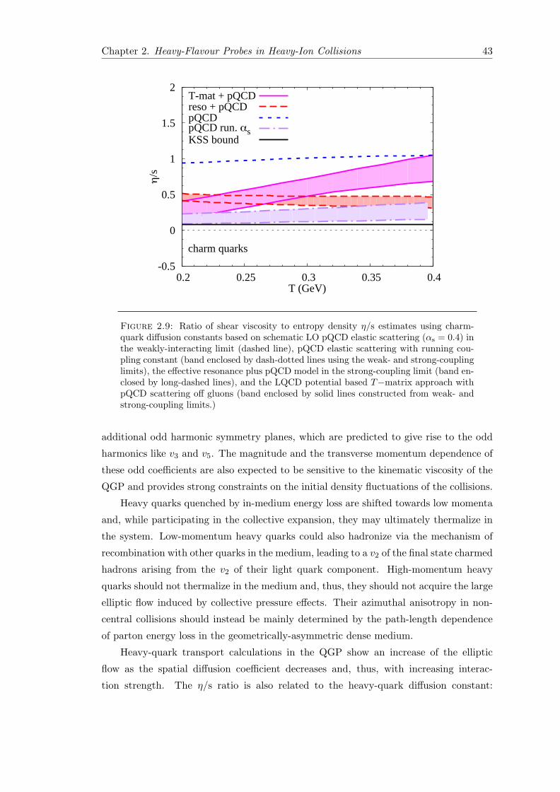
Chapter 2. Heavy-Flavour Probes in Heavy-Ion Collisions 43
August 1, 2009 6:56 WSPC/INSTRUCTION FILE hq-qgp4
Heavy quarks in the quark-gluon plasma 63
-0.5
0
0.5
1
1.5
2
0.2 0.25 0.3 0.35 0.4
η/s
T (GeV)
charm quarks
T-mat + pQCDreso + pQCDpQCDpQCD run. αsKSS bound
-0.5
0.0
0.5
1.0
1.5
2.0
1 1.5 2 2.5 3
243
8
163
8
s
KSS bound
PerturbativeTheory
T Tc
η
Fig. 29. (Color online) The ratio of shear viscosity to entropy density, η/s. Left panel: schematic
estimates using charm-quark diffusion constants based on (a) schematic LO pQCD elastic scatter-ing (αs=0.4) in the weakly interacting limit, Eq. (88) (dashed line), (b) pQCD elastic scatteringwith running coupling constant and small IR regulator (band enclosed by dash-dotted lines usingthe weak- and strong-coupling limits), (c) the effective resonance + pQCD model in the strong-coupling limit, Eq. (86) (band enclosed by long-dashed lines for Γ=0.4-0.75GeV), and (d) thelattice-QCD potential based T -matrix approach augmented by pQCD scattering off gluons (bandenclosed by solid lines constructed from the weak- and strong-coupling limits). Right panel: lat-tice QCD computations in a gluon plasma174 compared to results inferred from perturbationtheory175,176.
In comparison to the “strong-coupling” estimate within AdS/CFT, Eq. (86), the
shear viscosity appears to be underestimated when the kinetic theory for a dilute
gas is applied to liquids. These estimates are now applied to several of the HQ
diffusion calculations discussed above, see the left panel of Fig. 29. Since η/s ∝Ds(2πT ), the main features of Fig. 14 are transmitted to η/s, in particular the weak
temperature dependence of the LO-pQCD calculations and the effective resonance
model. Of course, the absolute values of these calculations differ considerably. A
different behavior is only found for the T -matrix+pQCD model, which suggests a
transition from a strongly coupled regime close to Tc to relatively weak coupling
above ∼2Tc. In fact, the uncertainty band has been constructed as follows: for the
lower limit, the weak-coupling estimate Eq. (88) is used; for the upper limit, the
strong-coupling limit estimate, Eq. (86), at T=0.2GeV is linearly interpolated with
the LO-pQCD weak-coupling limit at T=0.4GeV (the strong-coupling estimate for
T -matrix+pQCD overshoots the LO-pQCD result at this temperature). As for the
spatial diffusion constant, the increase of η/s with temperature is related to color-
Debye screening of the lQCD-based potentials which entails a gradual melting of the
dynamically generated resonances in the heavy-light quark T -matrix. It is tempting
to interpret the decrease of η/s when approaching Tc from above as a precursor-
phenomenon of hadronization and thus connected to the phase transition itself. It
remains to be seen whether a similar mechanism is operative in the light-quark
and/or gluon sector (three-body interactions are unlikely to produce this due to
the decrease in particle density when approaching Tc from above). Such a behavior
is rather general in that it has been observed around phase-transition points for a
Figure 2.9: Ratio of shear viscosity to entropy density η/s estimates using charm-quark diffusion constants based on schematic LO pQCD elastic scattering (αs = 0.4) inthe weakly-interacting limit (dashed line), pQCD elastic scattering with running cou-pling constant (band enclosed by dash-dotted lines using the weak- and strong-couplinglimits), the effective resonance plus pQCD model in the strong-coupling limit (band en-closed by long-dashed lines), and the LQCD potential based T−matrix approach withpQCD scattering off gluons (band enclosed by solid lines constructed from weak- andstrong-coupling limits.)
additional odd harmonic symmetry planes, which are predicted to give rise to the odd
harmonics like v3 and v5. The magnitude and the transverse momentum dependence of
these odd coefficients are also expected to be sensitive to the kinematic viscosity of the
QGP and provides strong constraints on the initial density fluctuations of the collisions.
Heavy quarks quenched by in-medium energy loss are shifted towards low momenta
and, while participating in the collective expansion, they may ultimately thermalize in
the system. Low-momentum heavy quarks could also hadronize via the mechanism of
recombination with other quarks in the medium, leading to a v2 of the final state charmed
hadrons arising from the v2 of their light quark component. High-momentum heavy
quarks should not thermalize in the medium and, thus, they should not acquire the large
elliptic flow induced by collective pressure effects. Their azimuthal anisotropy in non-
central collisions should instead be mainly determined by the path-length dependence
of parton energy loss in the geometrically-asymmetric dense medium.
Heavy-quark transport calculations in the QGP show an increase of the elliptic
flow as the spatial diffusion coefficient decreases and, thus, with increasing interac-
tion strength. The η/s ratio is also related to the heavy-quark diffusion constant:

Chapter 2. Heavy-Flavour Probes in Heavy-Ion Collisions 44
(GeV/c)T
p0 2 4 6 8 10 12 14 16 18 20
n v
0.1
0
0.1
0.2
0.3 (ALICE)2v (ALICE)
3v (ALICE)
4Ψ4/v (ATLAS)2v (ATLAS)
3v (ATLAS)
4Ψ4/v (CMS)2v (STAR)2v
= 2.76 TeVNNsALICE PbPb
3040%
ALI−DER−35551
Figure 2.10: Comparison of the ALICE results on vn(pT) to the analogous measure-ments from ATLAS and CMS collaborations, as well as v2 measurements by STAR [67–70].
η/s ∝ Ds(2πT ). The behaviour of the shear viscosity to entropy ratio as a func-
tion of temperature, as obtained considering different diffusion calculations, is reported
in Figure 2.9. A different behaviour is only found for the T−matrix+pQCD model,
which suggests a strongly-coupled regime close to Tc and a relatively weak coupling
above ∼ 2Tc. The increase of η/s with temperature is related to colour Debye screen-
ing of the LQCD-based potentials, which entails a gradual melting of the dynamically
generated resonances in the heavy-light quark T−matrix.
Elliptic Flow
The anisotropic flow coefficients are usually estimated from measured correlations be-
tween the observed particles. The anisotropic flow coefficients of charged particles were
measured at LHC for Pb–Pb collisions at√sNN = 2.76 TeV (Figure 2.10). The elliptic
(v2), triangular (v3) and v4 flow coefficients as a function of pT for non-central Pb–Pb
collisions are consistent among the LHC experiments [67–69]. v2 at top RHIC energy has
a peak value about 10% lower than at LHC although it is very similar in shape [70]. The
elliptic flow coefficient rises approximately linearly with pT to a maximum of v2 ≈ 0.23
around 3 GeV/c. The coefficient then decreases, but stays finite out of the highest pT
measured. Also the triangular flow coefficient is very significant out to about 10 GeV/c
and similar in shape, reaching about half the value of v2 at the maximum. The transverse

Chapter 2. Heavy-Flavour Probes in Heavy-Ion Collisions 45
33
[GeV/c]T
p0 0.5 1 1.5 2 2.5 3 3.5 4 4.5 5
HF
2v
−0.05
0
0.05
0.1
0.15
0.2
0−20%
[GeV/c]T
p0 0.5 1 1.5 2 2.5 3 3.5 4 4.5 5
HF
2v
−0.05
0
0.05
0.1
0.15
0.2
20−40%
[GeV/c]T
p0 0.5 1 1.5 2 2.5 3 3.5 4 4.5 5
HF
2v
−0.05
0
0.05
0.1
0.15
0.2
40−60%
[GeV/c]T
p0 0.5 1 1.5 2 2.5 3 3.5 4 4.5 5
HF
2v
−0.05
0
0.05
0.1
0.15
0.2
0−60%
FIG. 38: (Color online) vHF2 for the indicated centralities.
Mustafa [73] found that radiative and elastic scatter-ing energy loss for heavy quarks are comparable over avery wide kinematic range accessible at RHIC. Contraryto what was previously thought, collisional energy lossshould be taken into account in the calculation of sup-pression of heavy flavor mesons in Au+Au collisions. Fig-ure 39 shows the DGLV prediction for suppression whencollisional energy loss is taken into account in additionto radiative energy loss [72].In [74], it was shown that a Langevin-based heavy
quark transport model can qualitatively explain the largesuppression (and azimuthal anisotropy) of electrons fromheavy flavor decays in Au+Au collisions. The modelplaces a heavy quark into a thermal medium, and as-sumes that the interaction of the heavy quark with themedium can be described by uncorrelated momentumkicks. Contrary to the models described above, the inter-action in the Langevin model is given exclusively by elas-tic collisions, which is a good approximation for quarkswhich are not ultra-relativistic in the center of massframe of the collision. The parameter which is tuned inthis model is the heavy quark diffusion coefficient. Whilethe above Langevin model fails to simultaneously de-scribe RAA and v2 for a single value of the diffusion coef-
ficient, another Langevin-based model [75, 76] is in goodagreement with both the suppression and anisotropy. Inthis model, the elastic scattering is mediated by reso-nance excitation of D and B- like states in the medium.The theoretical evidence for the existence of such reso-nance states comes from lattice computations. Figure 40shows the calculations from these two models.Recently, it has been suggested that collisional disso-
ciation of heavy quarkonia in the quark-gluon plasma[77] may be a possible explanation for suppression ofJ/ψ production in heavy ion collisions. A. Adil andI. Vitev investigated the pQCD dynamics of open charmand bottom production and, in the framework of theGLV approach extended to composite qq systems, de-rived the medium induced dissociation probability forD and B mesons traveling through dense nuclear mat-ter [78]. They showed that the effective energy loss,which arises from the sequential fragmentation and dis-sociation of heavy quarks and mesons, is sensitive to theinterplay between the formation times of the hadrons andQGP and the detailed expansion dynamics of hot nuclearmatter. Figure 41 shows their result as the band.Most of the models calculate the nonphotonic electron
production assuming the same chemical composition of
Figure 2.11: Elliptic flow v2 of electrons coming from semileptonic decays of heavy-flavour mesons measured in Au–Au collisions at
√sNN = 200 GeV by PHENIX for
different collision centralities [44].
momentum dependence of v2 and v3 are described by hydrodynamical model calculations
with small value of the shear viscosity to entropy ratio η/s. The centrality dependence
of the elliptic and triangular flow was also investigated, and a significant difference was
observed. v3 does not depend strongly on centrality while v2 increases from central to
peripheral collisions. The strong change in v2 and the small change in v3 as a function of
centrality, in particular for the most central collisions, follow the centrality dependence
of the corresponding spatial anisotropies [71].
In the heavy-flavour sector, an azimuthal anisotropy in the production was observed
in Au–Au collisions at RHIC with v2 values of up to about 0.13 for electrons from heavy-
flavour decays, as shown in Figure 2.11 [44]. The results obtained at the LHC by ALICE
on D meson azimuthal anisotropy, which is one of the main goals of this thesis, will be
presented in Chapter 7.
2.4 Initial-State Effects and the Role of pA Collisions
A complete understanding of the nucleus–nucleus results requires an understanding of
the nuclear effects in the initial state, which can be accessed by studying proton–nucleus
collisions.

Chapter 2. Heavy-Flavour Probes in Heavy-Ion Collisions 46
0.2
0.6
1.0
1.5
10-3
10-2
10-1
1
ya
ye
xa xe
y0 shadowing
antishadowing
EMC-effect
Fermi-motion
Figure 1: An illustration of the fit function RAi (x) and the role of the parameters xa, xe, y0,
ya, and ye.
2.3 Experimental input and cross-sections
The main body of the data in our analysis consists of ℓ + A DIS measurements. Wealso utilize the DY dilepton production data from fixed target p+A collisions at Fermi-lab and inclusive neutral-pion production data measured in d+Au and p+p collisionsat RHIC1. Table 1 lists the sets included in our analysis and Fig. 2 displays theirkinematical reach in the (x,Q2)-plane. We will use the following notation:
RADIS(x,Q
2) ≡1AdσlA
DIS/dQ2dx
12dσld
DIS/dQ2dx
, RAF2(x,Q2) ≡ FA
2 (x,Q2)
F d2 (x,Q
2)
RADY(x1,2,M
2) ≡1AdσpA
DY/dM2dx1,2
12dσpd
DY/dM2dx1,2
(6)
RπdAu ≡ 1
⟨Ncoll⟩d2NdAu
π /dpTdy
d2Nppπ /dpTdy
min.bias=
12Ad2σdAu
π /dpTdy
d2σppπ /dpTdy
.
The kinematical variables in DIS are the Bjorken-x and the virtuality of the photon Q2.In DY M2 denotes the invariant mass of the lepton pair, and x1,2 ≡
!M2/s e±y where
y is the pair rapidity. The inclusive pion production is characterized by the transversemomentum pT and rapidity y of the outgoing pion. The average number of binarynucleon-nucleon collisions (in the centrality class studied) is denoted by ⟨Ncoll⟩. Inthis analysis we only consider minimum bias data, and do not focus on the transversecoordinate dependence of the nPDFs. The kinematical cuts we impose on the data areM2, Q2 ≥ 1.69GeV2 for DIS and DY, and pT ≥ 1.7GeV for inclusive pion production.
All cross-sections are calculated in the collinear factorization formalism folding the
1In contrast to our previous analysis [4], we do not include the BRAHMS forward rapidity chargedhadron d+Au data here. These data will be separately discussed in Sec. 4.
4
Figure 2.12: Illustration of the nuclear modification of bound nucleons.
Nuclear Modification of Parton Densities
The colliding nuclei do not behave as a mere incoherent superposition of their constituent
nucleons. In the initial state, the nuclear environment affects the quark and gluon
distributions, which are modified in bound nucleons depending on the parton fractional
momentum x and the atomic mass number A.
The bound nucleon PDFs fAi (x,Q2) for each parton flavour i are usually expressed
by
fAi (x,Q2) ≡ RAi (x,Q2)fi(x,Q2) , (2.18)
where RAi (x,Q2) denotes the nuclear modification to the free nucleon PDF fi(x,Q2).
Experiments of deep inelastic scattering (DIS) with nuclei have measured different nu-
clear effects associated to different ranges of x, illustrated in Figure 2.12: 1) shadowing
for the suppression observed at small x (x . 0.05); 2) antishadowing for the enhance-
ment at moderate values of x (0.05 . x . 0.3); EMC effect for the suppression observed
in the region 0.3 . x . 0.7; and 4) Fermi motion for the enhancement when x→ 1 [72].
As in the case of the free proton, the sets of nuclear PDFs are obtained by global fits
to several sets of experimental data. In Figure 2.13 a few sets for the ratios of PDFs
of protons inside a lead nucleus over those in a free proton are shown. The ratios are
rather similar for valence quarks, well constrained by the DIS data except at small x,
and sea quarks, constrained by DIS and Drell-Yan data except for very small and large
x. In the case of the gluons very different parametrizations lead to similar descriptions
of the available DIS and Drell-Yan data. The EPS09 [73] global fit analysis includes also
the results on pion production in d–Au and pp collisions at RHIC, which are sensitive
to the gluon distribution, and provides evidence for shadowing and EMC-effect also in
the nuclear gluons.

Chapter 2. Heavy-Flavour Probes in Heavy-Ion Collisions 47
2 4 6 8 10 12 14 160.7
0.8
0.9
1.0
1.1
1.2
1.3
1.4
PHENIX 20070
STAR 2006+
+-
EPS09NLO
[GeV]
RdA
u
y=0
Figure 9: The computed RdAu (thick black line and blue error band) at y = 0 for inclusivepion production compared with the PHENIX [28] data (open squares). The error bars are thestatistical uncertainties, and the yellow band indicate the point-to-point systematic errors.The additional 10% overall normalization uncertainty in the data is not shown. The datahave been multiplied by the optimized normalization factor fN = 1.03, which is an outputof our analysis. Also the STAR data [50] (open circles) multiplied by a normalization factorfN = 0.90 are shown for comparison.
0.20.40.60.81.01.21.4
0.20.40.60.81.01.21.4
10-4
10-3
10-2
10-1
10.00.20.40.60.81.01.21.4
10-4
10-3
10-2
10-1
10-4
10-3
10-2
10-10.0
0.20.40.60.81.01.21.4
This work, EPS09NLOHKN07 (NLO)nDS (NLO)
Q2=100 GeV
2
Q2=1.69 GeV
2
Pb Pb Pb
(,
2 =10
0G
eV2 )
Pb(
,2 =
1.69
GeV
2 )Pb
Figure 10: Comparison of the average valence and sea quark, and gluon modifications atQ2 = 1.69GeV2 and Q2 = 100GeV2 for Pb nucleus from the NLO global DGLAP analysesHKN07 [5], nDS [6] and this work, EPS09NLO.
18
Figure 2.13: Comparison of the average valence and sea quark, and gluon modifi-cations at Q2 = 1.69 GeV2 and Q2 = 100 GeV2 for Pb nucleus from different globalfits [73–75].
A direct consequence of shadowing is the reduction of hard-scattering cross sections
in the phase-space region characterized by small x incoming partons, hence, at midra-
pidity, low-pT outgoing partons. Charm and beauty production cross sections would
also be affected, in particular reduced, by this effect and the measurement of the nuclear
modification factor of the D meson pT distribution in p–Pb collisions at the LHC is a
sensitive tool to probe nuclear PDFs.
Nuclear-modified parton distribution functions allow to account for high-density ef-
fects at small x within the framework of perturbative QCD collinear factorization. How-
ever, factorization is expected to break down when the gluon density is large enough and
the gluon phase-space becomes saturated. In these conditions, partons in the nuclear
wave function at small x would act coherently, not independently as assumed with factor-
ization, and they may form a Color Glass Condensate (CGC). The relevant parameter in
the CGC is the saturation scale Q2s (x), determined by the parton density per unit trans-
verse area, and thus growing with the nuclear mass number A as Q2s (A) ∼ A/R2
A ∼ A1/3,
at fixed x. For a Pb nucleus probed at LHC energy, the estimated saturation scale at
x ∼ 10−4–10−5 is Q2s ∼ 2–3 GeV2 [76]. It has been argued that charm-quark production
in the kinematic domain corresponding to transverse masses smaller than the saturation
scale, mT,c . Qs ∼ 1.5–2 GeV, would be strongly affected by the presence of the CGC.
In particular, since the mean intrinsic transverse momentum of partons in the CGC is of

Chapter 2. Heavy-Flavour Probes in Heavy-Ion Collisions 48
the order Qs, rather than of the order ΛQCD ∼ 0.2 GeV as assumed in collinear factoriza-
tion, the fact that Qs � ΛQCD would lead to significantly harder transverse momentum
distributions for charm quarks in p–Pb than in pp collisions, and to a suppression of the
production for mT < Qs [77–80].
Initial State Multiple Scattering and Energy Loss
Partons can also lose energy in the initial stages of the collision via initial state radiation,
thus modifying the centre-of-mass energy of the partonic system, or experience transverse
momentum broadening due to multiple soft collisions before the cc pair is produced.
It was first observed in 1987 [81] that high-pT hadrons in pA collisions are produced
copiously in the range of pT . 2 GeV/c. This effect is know as Cronin effect and is
usually explained in terms of multiple interactions within the nucleus. The mechanism
of multiple interaction changes with energy. At low energies a high-kT parton is produced
off different nucleons incoherently, while at high energies it becomes a coherent process.
This is controlled by the coherence length
lc =
√s
mNkT, (2.19)
where kT is the transverse momentum of the parton produced at midrapidity and then
hadronizing into the detected hadron with transverse momentum pT. If the coherence
length is shorter than the typical nucleon–nucleon separation, the projectile interacts
incoherently with individual nucleons and the Cronin effect is due to soft multiple in-
teractions. If the coherence length is longer than the nuclear radius all amplitudes
interfere coherently and result in a collective parton distribution of the nucleus. In this
regime hard partons originate mainly from radiated gluons and the gluon shadowing is
responsible of a reduction of the Cronin effect [82–84].
Parton energy loss in nuclear matter shows a linear dependence on the path length
and on the energy for finite nuclei in the case of few interactions. The destructive
interference of gluons results to be less effective than in a hot medium in reducing
the total radiative energy loss with respect to a sum of single gluon emissions. In
AA collisions the final state energy loss is expected to be dominant with respect to
initial state one, due to the large density of the QGP, e.g. qcold ' 0.05 GeV2/fm,
qhot ' 10 GeV2/fm [85].
Possible Effects of Final State Flow
Recent studies on long-range correlations of charged hadrons in p–Pb collisions [86–89],
the measured species-dependent nuclear modification factor of pions, kaons, and protons
in d–Au collisions [90], and the larger suppression observed for the ψ′meson with respect

Chapter 2. Heavy-Flavour Probes in Heavy-Ion Collisions 494
(GeV/c) T
p0 1 2 3 4 5 6 7 8 9 10
)
2/ G
eV2
(pb
cT
d p
Tpσd
310
410
510
610
710
810
Blast Wave
FONLLD mesons
B mesons
(GeV/c) T
p0 1 2 3 4 5 6 7 8 9 10
dAu
R
0
0.5
1
1.5
2
2.5
3
3.5
D mesons Blast Wave + Binary Scaling
B mesons Blast Wave + Binary Scaling
FIG. 2. (left)D and B meson pT spectra from FONLL [41–43] (dashed lines) and from the blast-wave calculation presentedhere (solid lines). (right) The RdA from the comparison of the blast-wave and FONLL curves in the left panel with binaryscaling added at high pT . The dashed lines show the changes in the blast-wave expectations from the uncertainties on theblast-wave parameters discussed above.
(GeV/c) T
electron p0 2 4 6 8 10 12 14 16 18 20
(G
eV/c
)
TD
p
0
2
4
6
8
10
12
14
16
18
20
rela
tive
prob
abili
ty (
arb.
uni
ts)
0
0.1
0.2
0.3
0.4
0.5
0.6
0.7
0.8
0.9
1
(GeV/c) T
electron p0 2 4 6 8 10 12 14 16 18 20
(G
eV/c
)
TB
p
0
2
4
6
8
10
12
14
16
18
20
rela
tive
prob
abili
ty (
arb.
uni
ts)
0
0.1
0.2
0.3
0.4
0.5
0.6
0.7
0.8
0.9
1
FIG. 3. The relative probability to for a heavy meson to decayinto an electron at a given pT . D mesons are shown in theleft panel and B mesons are shown in the right panel. Thedecay kinematics are from PYTHIA8 [47].
5.02 TeV [42, 43]. Results for electrons and D mesons areshown in Figure 5. The D meson enhancement reachesa maximum of approximately 20% at pT ⇡ 3 GeV/c andthe electrons are enhanced by 10–20% nearly indepen-dently of pT over the range of 1–6 GeV/c. The calcu-lations are for the highest multiplicity event class andshow larger modifications than what would be expectedfor minimum bias collisions. Because of the harderD andB meson pT spectra at the higher collision energy thereis a smaller enhancement of heavy flavor mesons thanat RHIC, despite the larger maximal velocity extractedfrom the blast-wave fits.
(GeV/c) T
p0 1 2 3 4 5 6 7 8 9
dA
R
0
0.2
0.4
0.6
0.8
1
1.2
1.4
1.6
1.8
2
electrons, 0-20% PRL 109 242301 (2012)
Blast Wave calculation
FIG. 4. The heavy flavor decay electron RdA for 0-20% centrald+Au collisions from Ref. [37] (solid points) and from theblast-wave calculations presented in this work (curve). Thedashed lines show the changes in the blast-wave expectationsfrom the uncertainties on the blast-wave parameters discussedabove.
IV. CONCLUSIONS
Given the large uncertainties on the available heavyflavor data in d+Au collisions at RHIC and the large un-
(a)
5
(GeV/c) T
p0 1 2 3 4 5 6 7 8 9
pA
R
0
0.2
0.4
0.6
0.8
1
1.2
1.4
1.6
1.8
2
, p+Pb 5.02 TeV±HF e
D mesons, p+Pb 5.02 TeV
FIG. 5. Predictions for p+Pb collisions at 5.02 TeV. Blast-wave fit results from the 5% highest multiplicity p+Pb colli-sions [15] and FONLL [42, 43] heavy meson spectra have beenused to generate these results.
certainties on the blast-wave calculation here, it is impor-tant to consider how a radial flow interpretation of heavyflavor data in very small collision systems would be ver-ified or ruled out. The clearest evidence will come fromcharm and bottom separated results being made possi-ble by recently installed vertex detectors at both STAR
and PHENIX. Reconstructed D mesons from STARand charm and bottom separated electron measurementsfrom PHENIX will show the meson mass dependence ofthe heavy flavor enhancement seen by PHENIX [37]. Ad-ditionally, it is of interest to study multiplicity selectedp+p collisions at
ps = 200 GeV in order to investigate
how the blast-wave parameters evolve with both collisionsystem and event activity and how that informs the in-terpretation of the d+Au data discussed here in terms ofradial flow.
Recently, there has been much interest in the possibil-ity of hydrodynamic flow in very small collisions systems.Here we have raised the possibility that the enhancementof heavy flavor decay electrons previously observed [37]could be caused by radial flow using a blast-wave param-eterization constrained by the light hadron data. We findqualitative agreement between the data and the predic-tion of this model, suggesting hydrodynamics as one pos-sible explanation of the enhancement of electrons fromheavy flavor decay observed in d+Au collisions. Furthermeasurements have the potential to constrain any possi-ble role of hydrodynamics in very small collision systems.D meson spectra at RHIC are especially interesting as themodifications should be significantly larger than is seenat the LHC.
V. ACKNOWLEDGMENTS
The author thanks Dave Morrison, Paul Stankus andJamie Nagle for helpful conversations. The author is sup-ported by the U.S. Department of Energy under contractDE-AC02-98CH10886.
[1] U. W. Heinz and R. Snellings, Annu. Rev. Nucl. Part.Sci. 63, 123 (2013), arXiv:1301.2826 [nucl-th].
[2] A. Adare et al. (PHENIX Collaboration), Phys.Rev.Lett.107, 252301 (2011), arXiv:1105.3928 [nucl-ex].
[3] C. Gale, S. Jeon, B. Schenke, P. Tribedy, andR. Venugopalan, Nucl.Phys.A904-905 2013, 409c (2013),arXiv:1210.5144 [hep-ph].
[4] M. Luzum and J.-Y. Ollitrault, Nucl.Phys.A904-9052013, 377c (2013), arXiv:1210.6010 [nucl-th].
[5] P. Kovtun, D. Son, and A. Starinets, Phys.Rev.Lett. 94,111601 (2005), arXiv:hep-th/0405231 [hep-th].
[6] B. Abelev et al. (ALICE Collaboration), Phys.Lett.B719, 29 (2013), arXiv:1212.2001.
[7] G. Aad et al. (ATLAS Collaboration), Phys.Rev.Lett.110, 182302 (2013), arXiv:1212.5198 [hep-ex].
[8] A. Adare et al. (PHENIX Collaboration), Phys.Rev.Lett.(2013), arXiv:1303.1794 [nucl-ex].
[9] P. Bozek, Phys.Rev. C85, 014911 (2012),arXiv:1112.0915 [hep-ph].
[10] A. Bzdak, B. Schenke, P. Tribedy, and R. Venugopalan,(2013), 10.1103/PhysRevC.87.064906, arXiv:1304.3403[nucl-th].
[11] G.-Y. Qin and B. Mller, (2013), arXiv:1306.3439 [nucl-th].
[12] K. Dusling and R. Venugopalan, Phys.Rev. D87, 094034(2013), arXiv:1302.7018 [hep-ph].
[13] L. Van Hove, Phys.Lett. B118, 138 (1982).[14] S. Chatrchyan et al. (CMS Collaboration), (2013),
arXiv:1307.3442 [hep-ex].[15] B. B. Abelev et al. (ALICE Collaboration), (2013),
arXiv:1307.6796 [nucl-ex].[16] A. Bzdak and V. Skokov, (2013), arXiv:1306.5442 [nucl-
th].[17] P. Bozek, W. Broniowski, and G. Torrieri, (2013),
arXiv:1307.5060 [nucl-th].[18] P. Kolb, P. Huovinen, U. W. Heinz, and H. Heiselberg,
Phys.Lett. B500, 232 (2001), arXiv:hep-ph/0012137[hep-ph].
[19] E. Schnedermann, J. Sollfrank, and U. W. Heinz,Phys.Rev. C48, 2462 (1993), arXiv:nucl-th/9307020[nucl-th].
[20] B. Abelev et al. (STAR Collaboration), Phys.Rev. C79,034909 (2009), arXiv:0808.2041 [nucl-ex].
[21] J. Adams et al. (STAR Collaboration), Phys.Rev. C72,014904 (2005), arXiv:nucl-ex/0409033 [nucl-ex].
(b)
Figure 2.14: (a)RdA obtained from the comparison of the blast-wave and FONLL [34–36] D and B meson pT distributions with binary scaling. The dashed lines show thechanges in the blast-waves expectations from the uncertainties on the blast-wave param-eters. (b) RpA predicted for p–Pb collisions at
√sNN = 5.02 TeV. Blast-wave fit results
from the 5% highest multiplicity p–Pb collisions [95] and FONLL [34–36] heavy-mesonspectra have been used to generate these results [93].
to the J/ψ in both d–Au [91] and p–Pb [92] collisions, suggest the presence of final state
effects in small collision systems. These observations can be described in terms of an
hydrodynamically expanding medium. Some of them can also be described with a Color
Glass Condensate model. A possible hydrodynamic behaviour of heavy quarks in d–Au
and p–Pb collisions has been investigated using a blast-wave model [93]. This model
assumes thermalization and expansion with a common velocity field to describe the pT
distributions of particles. The parameters of the blast-wave (flow velocity β, and freeze-
out temperature) were extracted from the fits to the identified particle pT distributions
measured in d–Au [94] and p–Pb collisions [95], then the heavy-flavour meson spectra
were determined using the extracted parameters and the D and B meson masses. In order
to quantify the nuclear modification factor for heavy mesons expected from the blast
wave, the nuclear modification factor with respect to the FONLL [34–36] pT distribution
was calculated.
Figure 2.14 shows the nuclear modification factors RdA and RpPb that result from
the model. A large enhancement of D mesons, approximately of a factor two, is observed
at pT ≈ 2 GeV/c in d–Au collisions. A smaller enhancement (of a factor of about 1.8)
is observed for B mesons at pT ≈ 5 GeV/c (Figure 2.14(a)). The prediction for p–Pb
collisions at√sNN = 5.02 TeV is obtained using the blast-wave parameters extracted
from the 5% highest multiplicity events [95]. The D meson enhancement reaches a max-
imum of approximately 20% at pT ∼ 3 GeV/c and the electrons from heavy-flavour
decays are enhanced by 10–15%, nearly independently of pT over the range 1–6 GeV/c

Chapter 2. Heavy-Flavour Probes in Heavy-Ion Collisions 50 6
[GeV/c] T
p0 1 2 3 4 5 6 7 8 9
dA
, RA
AR
0.5
1
1.5
2
[GeV/c] T
p0 1 2 3 4 5 6 7 8 9
dA
, RA
AR
0.5
1
1.5
2dARHF
±e
AARHF ±e
dA R0π
AA R0π
FIG. 3: (color online) The nuclear modification factors RdA
and RAA for minimum bias d+Au and Au+Au collisions, forthe π0 and e±HF. The two boxes on the right side of theplot represent the global uncertainties in the d+Au (left) andAu+Au (right) values of Ncoll. An additional common globalscaling uncertainty of 9.7% on RdA and RAA from the p+preference data is omitted for clarity.
the d+Au yield by the p+p yield from [23]. At highertransverse momentum, where the p+p heavy-flavor elec-tron spectrum is consistent with a shape from pQCD,a fit to the spectral shape from the [24] calculations isused to represent the p+p yield. The statistical uncer-tainty on the fit is included as a systematic uncertaintyon the shape of RdA by adding it in quadrature with thesystematic uncertainties on the electron background sub-traction and solid angle and efficiency corrections. Theglobal scaling uncertainty from the uncertainty in Ncoll
and the total sampled p+p luminosity is given by a boxon the right. Note that the 2008 p+p data shown in Fig. 1could be used for the denominator of RdA, however, theuse of the more precise data from [23] gives a smalleruncertainty on RdA.
The central RdA shows an enhancement out to pT ≈ 5GeV/c, and implies that the suppression of heavy flavorelectrons in central Au+Au collisions at RHIC is not aninitial state CNM effect, but rather is due to the hot nu-clear medium. The peripheral nuclear modification fac-tor also shows some evidence of an enhancement, whichis to be expected since even the most peripheral central-ity bin in d+Au samples a significant nuclear thickness.Although the techniques used here do not allow sepa-ration of electrons from charm and bottom decays fromeach other, measurements from p+p show that pT = 5GeV/c is near the transition point where contributionsfrom bottom quarks begin to dominate over charm [25].Since the total charm cross section is expected to scalewith Ncoll, this enhancement below 5 GeV/c suggests apT broadening of the D spectral shape, with a mass de-pendence that roughly follows the previously observedtrend in the π,K, and p families. The B spectrum may
also be modified, however, the uncertainties on the dataand on the relativeD and B contributions to the electronspectra preclude a precise determination of any effects.
The effects of cold nuclear matter are expected to bepresent in the initial state of A+A collisions, however,this CNM enhancement is convolved with the suppress-ing effects of hot nuclear matter. Figure 3 shows RdA andRAA for e±HF and the neutral pion, for which only smallCNM effects are observed [19, 26]. Above pT ≈ 5 GeV/c,where the CNM effects on both species are small, theirRAA values are consistent within uncertainties. How-ever, in the range where CNM enhancement is large fore±HF and small on π0, the corresponding e±HFRAA valuesare consistently above the π0 values. This could suggestthat the difference in the initial state cold nuclear mattereffects due to the mass-dependent Cronin enhancementis reflected in the final state spectra of these particlesin Au+Au collisions, although alternate explanations in-volving mass-dependent partonic energy loss in the hotmedium are not ruled out.
In summary, we have observed an enhancement of elec-trons from heavy-flavor decays produced in central d+Aucollisions at
√sNN
= 200 GeV. The previously observedsuppression of these electrons in central Au+Au collisionsis therefore attributed to hot-nuclear-matter effects. Wefind that the π0 and e±HF nuclear modification factorsRAA are consistent within uncertainties in the pT rangewhere CNM effects on both species are small. In therange where CNM enhancement of e±HF is significant ind+Au, these effects may also be apparent in the Au+Audata.
We thank the staff of the Collider-Accelerator andPhysics Departments at Brookhaven National Labora-tory and the staff of the other PHENIX participatinginstitutions for their vital contributions. We acknowl-edge support from the Office of Nuclear Physics in theOffice of Science of the Department of Energy, the Na-tional Science Foundation, Abilene Christian UniversityResearch Council, Research Foundation of SUNY, andDean of the College of Arts and Sciences, Vanderbilt Uni-versity (U.S.A), Ministry of Education, Culture, Sports,Science, and Technology and the Japan Society for thePromotion of Science (Japan), Conselho Nacional de De-senvolvimento Cientıfico e Tecnologico and Fundacao deAmparo a Pesquisa do Estado de Sao Paulo (Brazil), Nat-ural Science Foundation of China (P. R. China), Min-istry of Education, Youth and Sports (Czech Repub-lic), Centre National de la Recherche Scientifique, Com-missariat a l’Energie Atomique, and Institut Nationalde Physique Nucleaire et de Physique des Particules(France), Bundesministerium fur Bildung und Forschung,Deutscher Akademischer Austausch Dienst, and Alexan-der von Humboldt Stiftung (Germany), Hungarian Na-tional Science Fund, OTKA (Hungary), Department ofAtomic Energy and Department of Science and Technol-ogy (India), Israel Science Foundation (Israel), National
Figure 2.15: The nuclear modification factors for minimum-bias d–Au and Au–Aucollisions for π0 and heavy-flavour electrons [96].
(Figure 2.14(b)). Because of the harder D and B meson pT distributions at the higher col-
lision energy, this calculation results in a smaller enhancement of heavy-flavour mesons
at LHC energy than at RHIC energy, despite the larger maximal velocity extracted from
the blast-wave fit.
Measurement of Heavy-Flavour Production in d–Au Collisions
at RHIC
Initial state effects, due to cold nuclear matter, in heavy-flavour production were inves-
tigated at RHIC by measuring the production of electrons from heavy-flavour hadron
decays in d–Au collisions at√sNN = 200 GeV. PHENIX measured an enhancement of
about 40% of the heavy-flavour decay electrons in the 20% most central d–Au collisions
with respect to pp collisions out to pT ≈ 5 GeV/c [96]. This enhancement suggests a pT
broadening of the D spectral shape, which depends on the mass of the particle (pions
which are much lighter than heavy-flavour mesons are less enhanced).
The nuclear matter effects are expected to be present also in the initial state of AA
collisions, however, combined with final state effects induced by the hot medium. The
comparison of the nuclear modification factor measured at RHIC in d–Au and Au–Au
collisions for electrons coming from heavy-flavour decays suggests that the suppression
observed in AA collisions is mainly due to hot medium effects, as can be argued from

Chapter 2. Heavy-Flavour Probes in Heavy-Ion Collisions 51
Figure 2.15 [96]. At the LHC, initial state effects in charm production were investigated
in p–Pb collisions at√sNN = 5.02 TeV, and the measurement is presented in Chapter 8
as one of the main results of this thesis.
2.5 Objective of the Thesis
Heavy quarks are valuable probes of the medium produced in ultra-relativistic collisions
of heavy nuclei. The fact that their masses are well above the typical temperature of
the system has at least three important implications, which allow to investigate different
aspects of their interaction with the medium:
1. The heavy-quark production process is restricted to primordial nucleon–nucleon
collisions and can be described with a perturbative QCD approach. Re-interactions
in the subsequently evolving medium are not expected to change the multiplicity
of heavy quarks.
2. The thermal relaxation time of heavy quarks is predicted to be larger than the
QGP lifetime, thus, they are not expected to reach thermal equilibrium, but their
interactions should modify the initial momentum spectrum. The final heavy-quark
spectra may therefore encode a memory of the interaction history throughout the
evolving fireball.
3. The energy loss of heavy quarks in the QGP is expected to be different with
respect to the one of light quarks and gluons. In particular, gluon bremsstrahlung
is predicted to be suppressed at small angles reducing the energy lost by a charm
(beauty) quark with respect to a light quark. Collisional (elastic) processes can
be related to the transport coefficients of the medium through a Brownian motion
treatment.
The results obtained on heavy-flavour production in pp, pA and AA collisions at
RHIC and LHC colliders, using D mesons and leptons from heavy-flavour semileptonic
decays have shown that:
• The production cross section in pp collisions is described by models implement-
ing the factorization approach with perturbative hard parton–parton interaction
description.
• The QGP formation induces a modification of the transverse momentum spectrum
of final state particles, in particular heavy-flavour mesons yields are suppressed at
high pT in Pb–Pb collisions with respect to pp collisions, consistently with a mass
dependent energy loss in the medium.
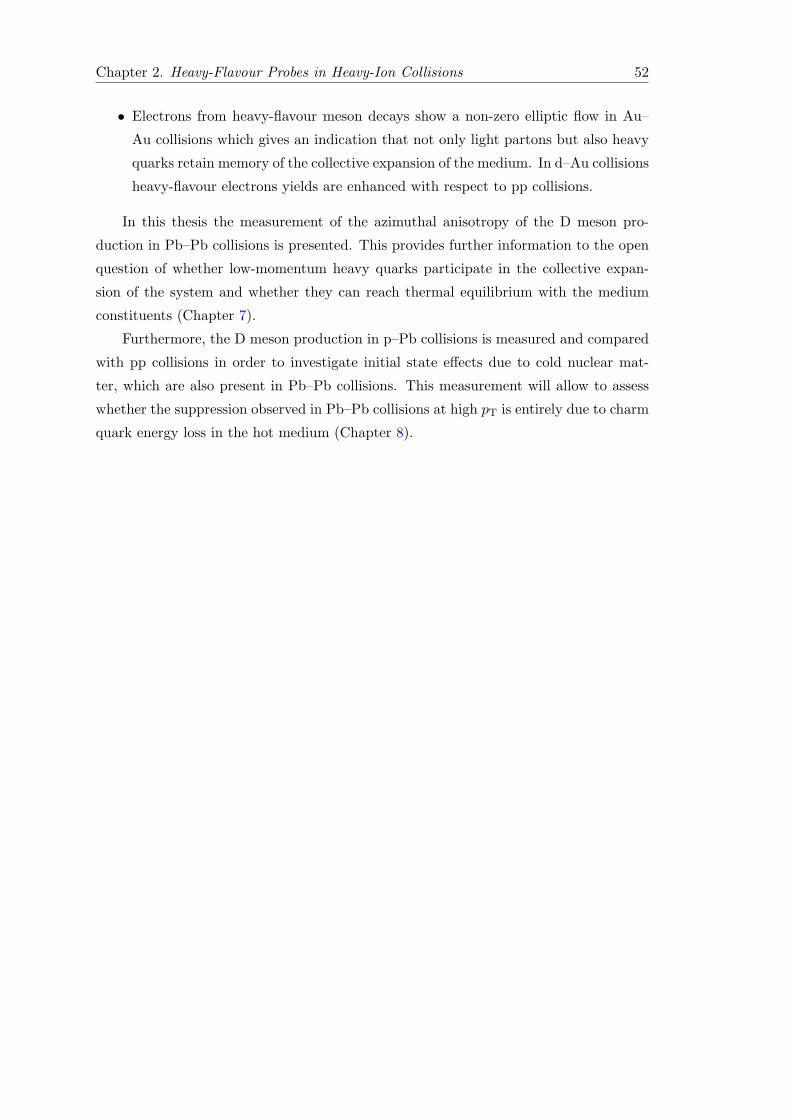
Chapter 2. Heavy-Flavour Probes in Heavy-Ion Collisions 52
• Electrons from heavy-flavour meson decays show a non-zero elliptic flow in Au–
Au collisions which gives an indication that not only light partons but also heavy
quarks retain memory of the collective expansion of the medium. In d–Au collisions
heavy-flavour electrons yields are enhanced with respect to pp collisions.
In this thesis the measurement of the azimuthal anisotropy of the D meson pro-
duction in Pb–Pb collisions is presented. This provides further information to the open
question of whether low-momentum heavy quarks participate in the collective expan-
sion of the system and whether they can reach thermal equilibrium with the medium
constituents (Chapter 7).
Furthermore, the D meson production in p–Pb collisions is measured and compared
with pp collisions in order to investigate initial state effects due to cold nuclear mat-
ter, which are also present in Pb–Pb collisions. This measurement will allow to assess
whether the suppression observed in Pb–Pb collisions at high pT is entirely due to charm
quark energy loss in the hot medium (Chapter 8).
3The ALICE Experiment at the LHC
A Large Ion Collider Experiment (ALICE) is one of the four large experiments at the
Large Hadron Collider (LHC), the accelerator built at CERN where protons and Pb
ions are accelerated to the highest energies ever reached. This chapter is devoted to
the description of ALICE, which is the experiment dedicated to the study of the Quark-
Gluon Plasma. In Section 3.1 the LHC main features are introduced, together with some
parameters of the proton and heavy-ion beams that are relevant for the study presented
in this thesis. An overview of the ALICE setup is given in Section 3.2, focusing on
the detectors that are used for the reconstruction of D meson decays. Section 3.3 and
Section 3.4 are devoted to the description of the ALICE tracking strategy and of the
particle identification signals and techniques which allow to deal with the extremely-high
multiplicity environment of Pb–Pb collisions. In Section 3.5 one of the most important
variables for the reconstruction of heavy-flavour particles, the track impact parameter,
is described.
3.1 The LHC Accelerator
The LHC is a superconducting accelerator and collider for hadrons with a circumference
of approximately 27 km. It is made of two rings with counter-rotating beams. It was built
to produce the highest energy proton–proton collisions ever performed, with the aim of
the discovery of the Higgs boson, which was actually announced the 4th of July 2012 by
the two experiments ATLAS [97] and CMS [98], and of the search of rare events beyond
the Standard Model. In addition to the proton beams, the LHC accelerates also heavy-
ion beams in order to study QCD matter created in ultra-relativistic heavy-ion collisions.
The LHC design energies are√s = 14 TeV for pp collisions and
√sNN = 5.5 TeV for
Pb–Pb collisions [99].
53

Chapter 3. The ALICE Experiment at the LHC 54
Figure 3.1: The CERN’s accelerator complex.
3.1.1 Acceleration Chain
The LHC is supplied with protons and Pb ions from a complex system of accelerators,
which is represented in Figure 3.1. Each machine boosts the energy of a beam of particles,
before injecting the beam into the next machine in the sequence. The proton source is
a tank of hydrogen gas. The hydrogen is passed through an electric field to strip off its
electrons, leaving only protons to enter the accelerator. Linear Accelerator 2 (Linac 2),
the first accelerator in the chain, accelerates protons to the energy of 50 MeV. The
beam is then injected into the Proton Synchrotron Booster (PSB), which accelerates
protons to 1.4 GeV, followed by the Proton Synchrotron (PS), which pushes the beam
to 25 GeV. Protons are then sent to the Super Proton Synchrotron (SPS) where they
are accelerated to 450 GeV. The proton are finally transferred to the two beam pipes of
the LHC where the beams have been accelerated up to 4 TeV up to now (2012) [99].
Lead ions for the LHC start from a source of vaporized lead and enter Linear Ac-
celerator 3 (Linac 3) before being collected and accelerated in the Low Energy Ion Ring
(LEIR). They then follow the same route to maximum energy (of 1.38 TeV per nucleon
up to now) as the protons [99].
The two beams are brought into collision inside the four experiments which are
installed on the LHC ring. ATLAS and CMS are the two experiments designed to
investigate a wide range of physics, including the search for the Higgs boson, extra
dimensions, and particles that could make up dark matter. The LHCb experiment is
Chapter 3. The ALICE Experiment at the LHC 55
specialized in investigating CP-violation mainly through B physics channels. ALICE
is the dedicated heavy-ion experiment and it is designed to study strongly-interacting
matter at extreme energy density, namely the QGP formation and properties.
3.1.2 pp, p–Pb and Pb–Pb Collisions
Since the main objective of the LHC physics programme is the exploration of rare
events, the main requirement of the machine is to deliver a large number of collisions.
The number of events per second (rate R) generated in the LHC collisions is given by:
R = Lσevent , (3.1)
where σevent is the cross section for the event under study and L the machine luminosity.
The machine luminosity depends only on the beam parameters and can be written for
a Gaussian beam distribution as:
L =N2
bnbfrevγr4πεnβ∗
F , (3.2)
where Nb is the number of particles per bunch, nb the number of bunches per beam, frev
the revolution frequency, γr the relativistic gamma factor, εn the normalized transverse
emittance1, β∗ the beta function2 at the collision point and F the geometric luminosity
reduction factor due to the crossing angle at the interaction point:
F =
(1 +
(θcσz2σ∗
))−1/2
, (3.3)
where θc is the full crossing angle at the interaction point, σz the RMS bunch length,
and σ∗ the transverse RMS beam size at the interaction point. The investigation of rare
phenomena in the LHC collisions therefore requires both high beam energies and high
beam intensities. The LHC design foresees 2802 bunches per beam in the ring with 25 ns
spacing between them. The nominal intensity is of around 1011 protons per bunch.
ATLAS and CMS are the two high luminosity experiments, aiming in proton–proton
collisions at a peak luminosity of 1034 cm−2s−1. LHCb aims at a peak luminosity
1032 cm−2s−1, and ALICE at a peak luminosity of 1027 cm−2s−1 for nominal lead-lead
operation [99].
1The emittance measures the average spread of particle coordinates in position and momentum phasespace. A low emittance particle beam is a beam where the particles are confined to a small distanceand have nearly the same momentum. The emittance is inversely proportional to the beam momentum:increasing the momentum of the beam reduces the emittance and hence the physical size of the beam. Itis often more useful to consider the normalized emittance εn = βγε, which does not change as a functionof energy.
2The amplitude function β(z) describes the single-particle motion and determines the variation ofthe beam envelope as a function of the coordinate along the the beam orbit, z. β∗ denotes the value ofthe beta function at the interaction point.

Chapter 3. The ALICE Experiment at the LHC 56
(a) (b)
Figure 3.2: LHC delivered integrated luminosity to the experiments during 2011Pb–Pb run (a) and during 2013 p–Pb run [100].
The luminosity in the LHC is not constant over a physics run but decays due to the
degradation of intensities and emittances of the circulating beams. The main cause for
the luminosity decay for nominal LHC performance are the collisions themselves.
The integral of the luminosity over time is called integrated luminosity and repre-
sents a measurement of the collected data size.
The LHC started its operation, the LHC Run 1, at the beginning of 2010 colliding
proton beams at the energy of√s = 7 TeV. Pb–Pb collisions were also delivered at the
energy of√sNN = 2.76 TeV per nucleon pair. The centre-of-mass energy for a nucleon–
nucleon collision, when two beams of nuclei (Z1, A1) and (Z2, A2) are accelerated with
the same magnetic rigidity, is obtained from the formula
√sNN =
√Z1Z2
A1A2
√s . (3.4)
In 2011 the proton and lead beam energy remained at 3.5 TeV and 1.38 TeV,
respectively. The Pb–Pb run was characterized by a factor 10 higher peak luminosity
with respect to the 2010 value, which translates to an integrated luminosity of about
150 µb−1 for ALICE, ATLAS, and CMS (Figure 3.2(a)) [100]. An increase in proton
beam energy to 4 TeV marked the start of operations in 2012. LHC Run 1 was completed
with a successful proton-lead run at the beginning of 2013 with beams of energy of 4 TeV
and 1.58 TeV, respectively. ATLAS, CMS, and ALICE were able to collect 31 nb−1 of
integrated luminosity, as reported in Figure 3.2(b) [100].
The results presented in this thesis were obtained with data samples collected during
the 2011 Pb–Pb run and 2013 p–Pb run. While pp and Pb–Pb are symmetric collisions
for which the centre-of-mass frame coincides with the laboratory frame, p–Pb collisions

Chapter 3. The ALICE Experiment at the LHC 57
Figure 3.3: The ALICE experiment at the CERN LHC. The central-barrel detectorsare embedded in a solenoid with magnetic field B = 0.5 T and address particle pro-duction at midrapidity. The cosmic-ray trigger detector ACORDE is positioned on topof the magnet. Forward detectors are used for triggering, event characterization, andmultiplicity studies. The Muon Spectrometer covers −4.0 < η < −2.5.
are asymmetric due to the different energies per nucleon of the proton and the lead
beams. The nucleon–nucleon centre-of-mass system moves with a longitudinal rapidity
yCM = 0.465 in the proton beam direction. The rapidity shift is obtained from the
expression:
yCM =1
2ln
(Z1A2
Z2A1
), (3.5)
where (Z1, A1) = (1, 1) and (Z2, A2) = (82, 208) are the atomic and mass numbers of
the proton and lead nucleus, respectively.
3.2 The ALICE Apparatus
The ALICE design has been chosen to perform precise measurements of the properties
of strongly-interacting matter that is formed in nucleus–nucleus collisions at extreme
values of temperature and energy density.
3.2.1 General Detector Layout
The ALICE apparatus, sketched in Figure 3.3, has overall dimensions of 16×16×26 m3
and a total weight of about 10000 t. It was designed to cope with the particle densities
Chapter 3. The ALICE Experiment at the LHC 58
expected in central Pb–Pb at the LHC and, thus, has a high detector granularity, a low
momentum threshold pminT ≈ 0.1 GeV/c, and good particle identification capabilities up
to 20 GeV/c. The experiment is composed of seventeen detector systems, which can be
classified in three categories: central-barrel detectors, forward detectors, and the muon
spectrometer. Table 3.1 summarizes the acceptance and location of the various detector
systems [101].
The ALICE coordinate system is a right-handed orthogonal Cartesian system: the
origin is at the LHC Interaction Point 2, the z axis is parallel to the mean beam direction
at the Interaction Point 2 and points along the LHC Beam 2 (i.e. LHC anticlockwise),
the x axis is horizontal and points approximately towards the center of the LHC, the y
axis, consequently, is approximately vertical and points upwards.
The Central-Barrel Detectors
The central-barrel detectors are the Inner Tracking System (ITS), the Time Projection
Chamber (TPC), the Transition Radiation Detector (TRD), the Time Of Flight (TOF),
the Photon Spectrometer (PHOS), the Electromagnetic Calorimeter (EMCal), and the
High Momentum Particle Identification Detector (HMPID). They are embedded in a
solenoid magnet with B = 0.5 T. The first four detectors cover the full azimuth at
midrapidity (|η| . 0.9). The ITS and the TPC are the main detectors of ALICE for
the tracking of charged particles. The ITS is composed of six tracking layers, two
Silicon Pixel Detectors (SPD), two Silicon Drift Detectors (SDD), and two Silicon Strip
Detectors (SSD). The TPC has a 90 m3 drift volume filled with Ne–Co2 and is divided
into two parts by the central cathode, which is kept at −100 kV. The end plates are
equipped with multiwire proportional chambers (MWPC). In addition to tracking, SDD,
SSD and TPC provide charged-particle identification via measurement of the specific
ionization energy loss dE/dx. The TRD detector consists of six layers of MWPCs filled
with Xe–CO2, with a fiber/foam radiator in front of each chamber. It is used for charged-
particle tracking and for electron identification via transition radiation and dE/dx. The
TOF detector is used for charged particle identification at intermediate momenta. It is
based on Multigap Resistive Plate Chamber (MRPC) technology. Finally, the cylindrical
volume outside TOF is shared by two electromagnetic calorimeters with thickness of
∼ 20 X0 (radiation lengths) and ∼ 1 λint (nuclear interaction length), the high resolution
PHOS and the large-acceptance EMCal, along with the ring-imaging Cherenkov detector
HMPID, which has a liquid C6F14 radiator and a CsI photo-cathode for charged-hadron
identification at intermediate momenta.

Chapter 3. The ALICE Experiment at the LHC 59
Table 3.1: Summary of the ALICE detector subsystems. The acceptance in η iscalculated from the nominal interaction point and is 360◦ in azimuth, unless notedotherwise. The position is the approximate distance from the interaction point tothe face of the detector and corresponds to the radius for barrel detectors (inner andouter radius for the TPC and TRD) or the position along the beam (z coordinate) forthe others. The dimension corresponds to the total area covered by active detectorelements. The total number of independent readout channels is also indicated. In casethe detector is subdivided, the numbers refer to the individual components [101].
Detector Acceptance (η, ϕ) Position (m) Dimension (m2) Channels
ITS layer 1,2 (SPD) ±2, ±1.4 0.039, 0.076 0.21 9.8 M
ITS layer 3,4 (SDD) ±0.9, ±0.9 0.150, 0.239 1.31 133000
ITS layer 5,6 (SSD) ±0.97, ±0.97 0.380, 0.430 5.0 2.6 M
TPC ±0.9 at r = 2.8 0.848, 2.466 readout 32.5 m2 557568
±1.5 at r = 1.4 m Vol. 90 m3
TRD ±0.84 2.90, 3.68 716 1.2 M
TOF ±0.9 3.78 141 157248
HMPID ±0.6, 1.2◦ < ϕ < 58.8◦ 5.0 11 161280
PHOS ±0.12, 220◦ < ϕ < 320◦ 4.6 8.6 17920
EMCal ±0.7, 80◦ < ϕ < 187◦ 4.36 44 12672
ACORDE ±1.3, −60◦ < ϕ < 60◦ 8.5 42 120
Muon Spectrometer
Tracking station 1 −4.0 < η < −2.5 -5.36 4.7 1.08 M
Tracking station 2 -6.86 7.9
Tracking station 3 -9.83 14.4
Tracking station 4 -12.92 26.5
Tracking station 5 -14.22 41.8
Trigger station 1 −4.0 < η < −2.5 -16.12 64.6 21000
Trigger station 2 -17.12 73.1
ZDC:ZN |η| < 8.8 ±116 2×0.0049 10
ZDC:ZP 6.5 < η < 7.5 ±116 2×0.027 10
−9.7◦ < ϕ < 9.7◦
ZDC:ZEM 4.8 < η < 5.7 7.25 2×0.0049 2
−16◦ < ϕ < 16◦ and
164◦ < ϕ < 196◦
PMD 2.3 < η < 3.7 3.64 2.59 2221184
FMD disc 1 3.62 < η < 5.03 inner: 3.2
FMD disc 2 1.7 < η < 3.68 inner: 0.834 0.266 51200
outer: 0.752
FMD disc 3 −3.4 < η < −1.7 inner: -0.628
outer: -0.752
VZERO-A 2.8 < η < 5.1 3.4 0.548 32
VZERO-C −3.7 < η < −1.7 -0.897 0.315 32
T0A 4.61 < η < 4.92 3.75 0.0038 12
T0C −3.28 < η < −2.97 -0.727 0.0038 12
Chapter 3. The ALICE Experiment at the LHC 60
The Forward Detectors
The ALICE forward detectors include the preshower/gas-counter Photon Multiplicity
Detector (PMD) and the silicon Forward Multiplicity Detector (FMD), which are dedi-
cated to the measurement of photons and charged particles around η ≈ 3, respectively.
The quartz Cherenkov detector T0 delivers the time and the longitudinal position of the
interaction. It consists of two arrays of Cherenkov counters positioned at opposite sides
of the interaction point at −3.28 < η < −2.97 and 4.61 < η < 4.92. The plastic scintilla-
tor detector VZERO measures charged particles at −3.7 < η < −1.7 and 2.8 < η < 5.1,
and it is mainly used for triggering and for the determination of centrality and event-
plane angle in Pb–Pb collisions. The centrality can also be measured with the Zero
Degree Calorimeter (ZDC). The ZDC consists of two tungsten-quartz neutron (ZN) and
two brass-quartz proton (ZP) calorimeters, placed symmetrically on both sides of the
interaction point and used to count spectator nucleons.
The Muon Spectrometer
The Muon Spectrometer is used to measure heavy-flavour quarkonium and light vector
meson production in a region −4.0 < η < −2.5. It is also used to measure high-pT muons
which predominantly come from the decay of W bosons. The Muon Spectrometer is
made of a hadron absorber of about 10λint, a dipole magnet of 3 Tm, and five tracking
stations with two pad chambers each (Muon Chambers, MCH). Single-muon and muon-
pair triggers with an adjustable transverse momentum threshold are provided by two
further stations (Muon Trigger, MTR) placed behind an additional 7λint absorber.
The D mesons are reconstructed in the central rapidity region exploiting the track-
ing and particle identification capabilities of the ALICE central-barrel detectors. The
relevant detectors for the D meson analysis are the ITS, the TPC and the TOF: their
main features are described below.
3.2.2 ITS
The main tasks of the ITS are to localize the primary vertex with a resolution better
than 100 µm, to reconstruct the secondary vertices from the decays of hyperons and
D and B mesons, to track and identify particles with momentum below 200 MeV/c, to
improve the momentum and angle resolution for particles reconstructed by the TPC and
to reconstruct particles traversing dead regions of the TPC.
The ITS surrounds the beam pipe, which is a 800 µm-thick beryllium cylinder of
6 cm outer diameter, coaxial with the ITS detector layers. The ITS consists of six

Chapter 3. The ALICE Experiment at the LHC 61
cylindrical layers of silicon detectors, located at radii between 3.9 and 43 cm. It covers
the rapidity range of |η| < 0.9 for all vertices located within the length of the interaction
diamond (±1σ, i.e. ±5.3 cm along the beam direction).
The two innermost layers, with average radii of 3.9 cm (about 1 cm from the beam
vacuum tube) and 7.6 cm, are equipped with Silicon Pixel Detectors, comprising 9.8×10⁶
pixels of size 50(rϕ)×425(z) µm2, with intrinsic spatial resolution of 12(rϕ)×100(z) µm2.
The signals of the 1200 SPD readout chips provide a fast trigger through a programmable
logic. The two intermediate layers, at radii of 15.0 and 23.9 cm, are made of Silicon Drift
Detectors. The intrinsic spatial resolution of the third and fourth layers is of 35 µm in
rϕ direction and 25 µm in z direction. The two outermost layers are made of Silicon
Strip Detectors, located at radii of 38.0 and 43.0 cm, consisting of double-sided silicon
strip sensor modules, with an intrinsic spatial resolution of 20(rϕ) × 830(z) µm2. The
alignment of the ITS sensor modules is crucial for the precise space point reconstruction
needed for heavy-flavour analysis. It was performed using survey information, cosmic-
ray tracks and pp data. The effective spatial resolution along the most precise direction,
rϕ, is about 14, 40 and 25 µm for SPD, SDD and SSD, respectively [101].
The momentum and impact parameter (i.e. the distance of closest approach of the
track to the primary interaction vertex) resolution for low-momentum particles are dom-
inated by multiple scattering effects in the material of the detector; therefore the amount
of material in the active volume has been kept to a minimum. The total material budget
of the ITS is on average 7.7% of radiation length for tracks crossing the ITS perpendic-
ularly to the detector surfaces (η = 0).
3.2.3 TPC
The TPC is the main tracking detector of the central barrel and is optimized to provide,
together with the other central-barrel detectors, charged-particle momentum measure-
ments with good two-track separation, particle identification, and vertex determination.
The phase space covered by the TPC in pseudorapidity is |η| < 0.9 for tracks with
full radial track length; for reduced track length (at reduced momentum resolution) an
acceptance up to about |η| < 1.5 is accessible. The TPC covers the full azimuth (with
the exception of the dead zones). A large pT range is covered from low pT of about
0.1 GeV/c up to 100 GeV/c with good momentum resolution.
The TPC has a cylindrical shape; the active volume has an inner radius of about
85 cm, an outer radius of about 250 cm, and an overall length along the beam direction
of 500 cm.
The detector is made of a cylindrical field cage, filled with 90 m3 of Ne/CO2/N2
(90/10/5), in which the primary electrons are transported over a distance of up to
2.5 m on either side of the central electrode to the end plates. Multi-wire proportional

Chapter 3. The ALICE Experiment at the LHC 62
chambers with cathode pad readout are mounted into 18 trapezoidal sectors at each end
plate.
Charged-particle tracks are reconstructed and identified with up to 159 3-dimensional
space points. The TPC also provides particle identification capabilities through the
measurement of the specific energy deposition dE/dx, with up to 159 samples. Using
cosmic-ray muons and data taken in pp collisions, the relative dE/dx resolution was
measured to be about 5.5% for tracks that cross the entire detector [101].
3.2.4 TOF
The TOF detector is a large area array that covers the central pseudorapidity region
(|η| < 0.9) for Particle IDentification (PID) in the intermediate momentum range, below
about 2.5 GeV/c for pions and kaons, up to 4 GeV/c for protons, with a π/K and K/p
separation better than 3σ.
TOF is based on the Multi-gap Resistive-Plate Chambers in a cylindrical config-
uration at radius 370–399 cm from the beam axis, with readout consisting of 152928
sensitive pads of dimension 2.5× 3.5 cm2.
The TOF provides an arrival time measurement for charged tracks with an overall
resolution, including the measurement of the event start time, of about 80 ps for pions
and kaons at pT = 1 GeV/c [101]. The particle identification is based on the difference
between the measured time-of-flight and its expected value, computed for each mass
hypothesis from the track momentum and length.
3.3 Central-Barrel Tracking
The procedure of track finding in the central barrel starts with the clusterization step,
in which the detector data are converted into “clusters” characterized by positions,
signal amplitudes, signal times, etc., and their associated errors. The clusterization is
performed separately for each detector. The next step is a first reconstruction of the
interaction vertex using clusters in the first two ITS layers (SPD). Subsequently, track
finding and fitting is performed in TPC and ITS using the Kalman filter technique [102].
The found tracks are matched to the outer central-barrel detectors and fitted. The final
interaction vertex is determined using the reconstructed tracks.
3.3.1 Interaction Vertex Reconstruction with SPD
Tracking in the central barrel starts with the determination of the interaction vertex
using the two innermost layers (SPD) of the ITS. It is found as a space point to which

Chapter 3. The ALICE Experiment at the LHC 63
(GeV/c)T
p
0 2 4 6 8 10
TP
C e
ffici
ency
0
0.1
0.2
0.3
0.4
0.5
0.6
0.7
0.8
0.9
1
|<0.8 (MC)ηALICE |
=2.76 TeV, centrality 05% NNsPbPb
=2.76 TeV, centrality 8090%NNsPbPb
=8 TeVspp
ALI−PUB−70722
Figure 3.4: TPC track finding efficiency for primary particles in pp and Pb–Pbcollisions (simulation). The efficiency does not depend on the detector occupancy [103].
a maximum number of tracklets3 converge. In pp collisions, where interaction pileup
is expected, the algorithm is repeated several times, discarding at each iteration those
clusters which contributed to already-found vertices. By construction, the first vertex
found has the largest number of contributing tracklets and is assumed to be the primary
one. When a single convergence point is not found (in particular in low-multiplicity
events) the algorithm performs a one-dimensional search of the maximum in the z-
distribution of the points of closest approach of tracklets to the nominal axis.
3.3.2 Track Reconstruction
Track finding and fitting is performed in three stages, following an inward-outward-
inward scheme. The first inward stage starts with finding tracks in the TPC. The TPC
readout chambers have 159 tangential pad rows and thus a track can, ideally, produce
159 clusters within the TPC volume. The track search in the TPC starts at a large
radius. Track seeds are built first with two TPC clusters and the vertex point, then
with three clusters and without the vertex constraint. The seeds are propagated inward
and, at each step, updated with the nearest cluster provided that fulfils a proximity cut.
Only those tracks that have at least 20 clusters (out of maximum 159 possible) and that
miss no more than 50% of the clusters expected for a given track position are accepted.
These are propagated inwards to the inner TPC radius. The tracking efficiency, defined
as the ratio between the reconstructed tracks and generated primary particles in the
simulation, is shown in Figure 3.4 as a function of transverse momentum. The drop
3Tracklets are defined as the lines which connect a pair of clusters, one cluster in each SPD layer.
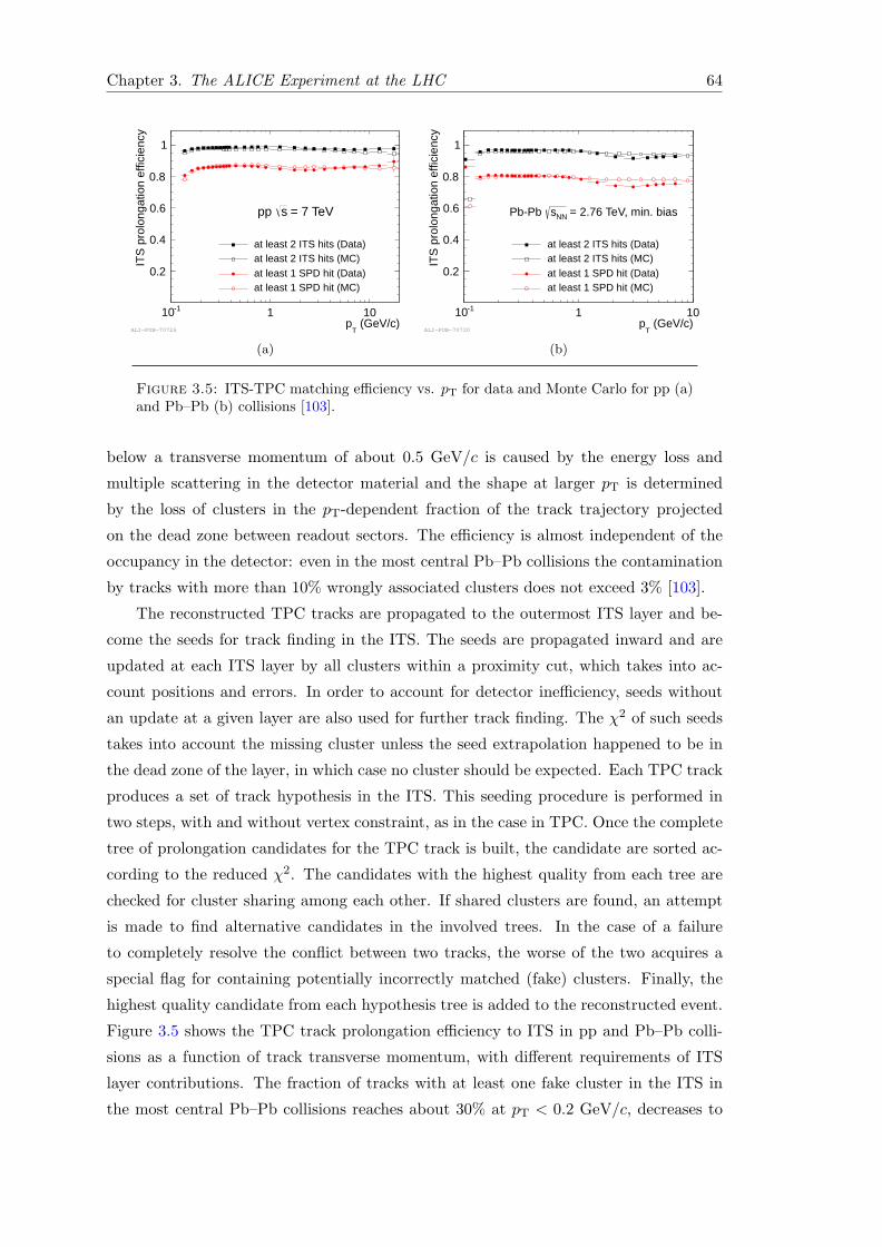
Chapter 3. The ALICE Experiment at the LHC 64
(GeV/c)T
p110 1 10
ITS
pro
long
atio
n ef
ficie
ncy
0.2
0.4
0.6
0.8
1
= 7 TeVspp
at least 2 ITS hits (Data)at least 2 ITS hits (MC)at least 1 SPD hit (Data)at least 1 SPD hit (MC)
ALI−PUB−70726
(a)
(GeV/c)T
p110 1 10
ITS
pro
long
atio
n ef
ficie
ncy
0.2
0.4
0.6
0.8
1
= 2.76 TeV, min. biasNNsPbPb
at least 2 ITS hits (Data)at least 2 ITS hits (MC)at least 1 SPD hit (Data)at least 1 SPD hit (MC)
ALI−PUB−70730
(b)
Figure 3.5: ITS-TPC matching efficiency vs. pT for data and Monte Carlo for pp (a)and Pb–Pb (b) collisions [103].
below a transverse momentum of about 0.5 GeV/c is caused by the energy loss and
multiple scattering in the detector material and the shape at larger pT is determined
by the loss of clusters in the pT-dependent fraction of the track trajectory projected
on the dead zone between readout sectors. The efficiency is almost independent of the
occupancy in the detector: even in the most central Pb–Pb collisions the contamination
by tracks with more than 10% wrongly associated clusters does not exceed 3% [103].
The reconstructed TPC tracks are propagated to the outermost ITS layer and be-
come the seeds for track finding in the ITS. The seeds are propagated inward and are
updated at each ITS layer by all clusters within a proximity cut, which takes into ac-
count positions and errors. In order to account for detector inefficiency, seeds without
an update at a given layer are also used for further track finding. The χ2 of such seeds
takes into account the missing cluster unless the seed extrapolation happened to be in
the dead zone of the layer, in which case no cluster should be expected. Each TPC track
produces a set of track hypothesis in the ITS. This seeding procedure is performed in
two steps, with and without vertex constraint, as in the case in TPC. Once the complete
tree of prolongation candidates for the TPC track is built, the candidate are sorted ac-
cording to the reduced χ2. The candidates with the highest quality from each tree are
checked for cluster sharing among each other. If shared clusters are found, an attempt
is made to find alternative candidates in the involved trees. In the case of a failure
to completely resolve the conflict between two tracks, the worse of the two acquires a
special flag for containing potentially incorrectly matched (fake) clusters. Finally, the
highest quality candidate from each hypothesis tree is added to the reconstructed event.
Figure 3.5 shows the TPC track prolongation efficiency to ITS in pp and Pb–Pb colli-
sions as a function of track transverse momentum, with different requirements of ITS
layer contributions. The fraction of tracks with at least one fake cluster in the ITS in
the most central Pb–Pb collisions reaches about 30% at pT < 0.2 GeV/c, decreases to

Chapter 3. The ALICE Experiment at the LHC 65
about 7% at 1 GeV/c, and drops below 2% at 10 GeV/c [103].
A standalone ITS reconstruction is performed with those clusters that were not used
in the ITS-TPC tracks. The algorithm adopted enables the tracking of particles with
transverse momenta down to about 80 MeV/c.
Once the reconstruction in the ITS is complete, all tracks are extrapolated to their
point of closest approach to the preliminary interaction vertex, and the outward prop-
agation starts. The tracks are refitted by the Kalman filter in the outward direction
using the clusters found at the previous stage. At each outward step, the track length
integral, as well as the time of flight expected for various particle species are updated
for subsequent particle identification. Once the track reaches the TRD, an attempt is
made to match it with the TRD tracklet (track segment within a TRD layer) in each
of the six TRD layers. Similarly, the tracks reaching the TOF detector are matched to
TOF clusters. The track length integration and time-of-flight calculation are stopped at
this stage. The tracks are then propagated further for matching with signals in EMCal,
PHOS, and HMPID. The detectors at a radius larger than that of TPC are currently
not used to update the measured track kinematics, but their information is stored in
the track object for the purposes of particle identification.
At the final stage of the track reconstruction, all tracks are propagated inwards
starting from the outer radius of the TPC. In each detector (TPC and ITS), the tracks
are refitted with the previously found clusters. The track’s position, direction, inverse
curvature, and its associated covariance matrix are determined.
Figure 3.6 shows the transverse momentum resolution for TPC standalone tracks
and ITS-TPC combined tracks extracted from the track covariance matrix. The effect of
constraining the tracks to the primary vertex is shown as well. The inverse-pT resolution
is connected to the relative transverse momentum resolution via
σpT
pT= pTσ1/pT
. (3.6)
Figure 3.6 is relative to the data taken in the recent p–Pb run, in central Pb–Pb collisions,
the pT resolution is expected to deteriorate by about 10% at high pT due to the loss (or
reduction) of clusters sitting on the ion tails, cluster overlap, and fake cluster attached to
the tracks [103]. Heavy-flavour analysis make use of the track parameters not constrained
to the primary vertex.
3.3.3 Final Reconstruction of the Interaction Vertex
The interaction vertex is found using global tracks reconstructed in TPC and ITS.
This method provides a better precision than the usage of SPD tracklets alone. By
extrapolating the tracks to the point of closest approach to the nominal beam line and

Chapter 3. The ALICE Experiment at the LHC 66
((GeV/c) )T
1/p
0 0.1 0.2 0.3 0.4 0.5 0.6 0.7 0.8 0.9 1
((G
eV
/c)
)T
1/p
m
0
0.002
0.004
0.006
0.008
0.01
0.012
0.014
0.016
|<0.8d = 5.02 TeV, |NN
sp-Pb,
TPC standalone tracks
TPC tracks constrained to vertex
TPC+ITS combined tracks
TPC+ITS constrained to vertex
-1
-1
ALICE
ALI-PUB-72271ALI-PUB-72271ALI-PUB-72271
Figure 3.6: The pT-resolution for standalone TPC and ITS-TPC matched tracks withand without constraint to the vertex. The vertex constraint significantly improves theresolution of TPC standalone tracks. For ITS-TPC tracks, it has no effect (green andblue squares overlap) [103].
removing far outliers, the approximate point of closest approach of validated tracks is
determined. Then the precise vertex fit is performed using track weighting to suppress
the contribution of any remaining outliers. In order to improve the transverse vertex
position precision in low-multiplicity events, the nominal beam position is added in the
fit as an independent measurement with errors corresponding to the transverse size of
the luminous region4. Figure 3.7 shows the profiles (x Figure 3.7(a) and z Figure 3.7(b))
of the luminous region obtained from reconstructed vertices in pp and Pb–Pb collisions.
The transverse resolution of the preliminary interaction vertices found with SPD and
of the final ones, found with global tracks, are shown in Figure 3.8. Both resolutions
scale with the inverse of the square root of the number of contributing tracks (tracklets),
which is proportional to the charged-particle multiplicity, dNch/dη.
3.4 Particle Identification
3.4.1 PID in the TPC
Particle identification in the TPC is performed by simultaneously measuring the specific
energy loss (dE/dx), charge, and momentum of each particle traversing the detector gas.
4The interaction region, or beam size, is defined as the convolution of the two particles distributionsin the two colliding bunches: the interaction vertex lies in a luminous region with dimensions σlumi reg
q =σbeamq /
√2 with q = x, y, z.
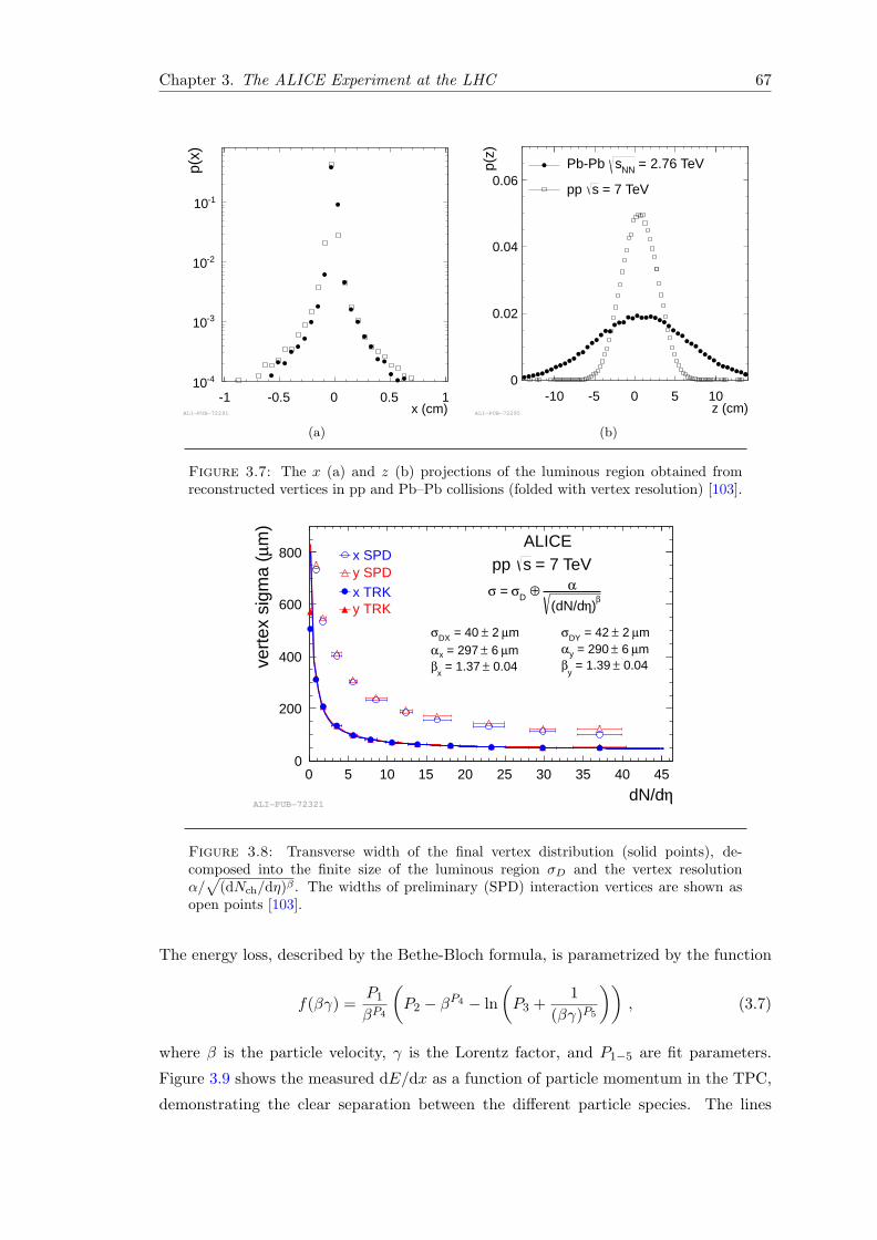
Chapter 3. The ALICE Experiment at the LHC 67
x (cm)1 0.5 0 0.5 1
p(x)
410
310
210
110
ALI−PUB−72291
(a)
z (cm)10 5 0 5 10
p(z)
0
0.02
0.04
0.06 = 2.76 TeVNNsPbPb
= 7 TeVspp
ALI−PUB−72295
(b)
Figure 3.7: The x (a) and z (b) projections of the luminous region obtained fromreconstructed vertices in pp and Pb–Pb collisions (folded with vertex resolution) [103].
ηdN/d0 5 10 15 20 25 30 35 40 45
m)
µve
rtex
sig
ma
(
0
200
400
600
800 x SPDy SPDx TRKy TRK
mµ 2 ± = 42 DYσ
mµ 6 ± = 290 yα
0.04± = 1.39 y
β
mµ 2 ± = 40 DXσ
mµ 6 ± = 297 xα
0.04± = 1.37 x
β
β)η(dN/d
α ⊕ Dσ = σ
ALICE = 7 TeVspp
ALI−PUB−72321
Figure 3.8: Transverse width of the final vertex distribution (solid points), de-composed into the finite size of the luminous region σD and the vertex resolutionα/√
(dNch/dη)β . The widths of preliminary (SPD) interaction vertices are shown asopen points [103].
The energy loss, described by the Bethe-Bloch formula, is parametrized by the function
f(βγ) =P1
βP4
(P2 − βP4 − ln
(P3 +
1
(βγ)P5
)), (3.7)
where β is the particle velocity, γ is the Lorentz factor, and P1−5 are fit parameters.
Figure 3.9 shows the measured dE/dx as a function of particle momentum in the TPC,
demonstrating the clear separation between the different particle species. The lines

Chapter 3. The ALICE Experiment at the LHC 68
)c (GeV/p0.2 0.3 1 2 3 4 5 6 7 8 910 20
(ar
b. u
nits
)x
/dE
TP
C d
20
40
60
80
100
120
140
160
180
200
π
e
K p dTeV 2.76 = NNsPbPb
ALI−PUB−72357
Figure 3.9: Specific energy loss (dE/dx) in the TPC vs. particle momentum in Pb–Pb collisions at
√sNN = 2.76 TeV. The lines show the parametrization of the expected
mean energy loss [103].
correspond to the parametrization. At low momenta (p . 1 GeV/c) particles can be
identified on a track-by-track basis. At higher momenta particles can still be separated
on a statistical basis via multi-Gaussian fits.
In the relativistic rise region, the dE/dx exhibits a nearly constant separation for
the different particle species over a wide momentum range. Due to a dE/dx resolution
of about 5.2% in pp collisions and 6.5% in the 0–5% most central Pb–Pb collisions,
particle ratios can be measured at a pT of up to 20 GeV/c [103].
3.4.2 PID in the TOF
The overall TOF time resolution in Pb–Pb collisions, in the centrality range 0–70%, is
80 ps for pions with a momentum around 1 GeV/c. This value includes the intrinsic
detector resolution, the contribution from electronics and calibration, the uncertainty on
the start time of the event, and the tracking and momentum resolution. TOF provides
PID in the intermediate momentum range, up to 2.5 GeV/c for pions and kaons, and
up to 4 GeV/c for protons.
The start time for the TOF measurement is provided by the T0 detector. The time
resolution of the detector is 20-25 ps in Pb–Pb collisions and about 40 ps in pp collisions.
The start time of the event is also estimated using the particle arrival times at the TOF
detector if at least three particles reach it. The method is particularly useful for events

Chapter 3. The ALICE Experiment at the LHC 69
1
10
210
310
410
510
)c (GeV/p0 0.5 1 1.5 2 2.5 3 3.5 4 4.5 5
βT
OF
0.1
0.2
0.3
0.4
0.5
0.6
0.7
0.8
0.9
1
1.1e
πK
p
d
TeV 2.76 = NNsPbPb
ALI−PUB−72381
(a)
1
10
210
310
410
)c (GeV/p0 0.5 1 1.5 2 2.5 3 3.5 4 4.5 5
βT
OF
0.1
0.2
0.3
0.4
0.5
0.6
0.7
0.8
0.9
1
1.1e
πK
p
d
TeV 5.02 = NNspPb
ALI−PUB−72385
(b)
Figure 3.10: Distribution of β as measured by the TOF detector as a function of mo-mentum for particles reaching TOF in Pb–Pb interaction (a) and in p–Pb interactions(b). The background of mismatched tracks is lower in p–Pb than in higher occupancyPb–Pb collisions [103].
in which the T0 signal is not present. If neither of these two methods is available an
average TOF start time for the run is used instead.
Figure 3.10 illustrates the performance of the TOF detector by showing the mea-
sured velocity β distribution as a function of the momentum (measured by the TPC).
The background is due to tracks that are incorrectly matched to TOF hits in high-
multiplicity collisions. The background is larger in Pb–Pb collisions (Figure 3.10(a))
while the distribution is cleaner in p–Pb collisions (Figure 3.10(b)), showing that the
background is not related to the resolution of the TOF detector, but is rather an effect of
track density and the fraction of mismatched tracks. The fraction of mismatched tracks
above 1 GeV/c in Pb–Pb events is closely related to the TOF occupancy. With 104 hits
at TOF (corresponding to a very central Pb–Pb event) the TOF pad occupancy is 6.7%
and the fraction of mismatched hits is about 6.5% [103].
The resolution can be studied in a given narrow momentum interval by computing
the difference between the time of flight measured by TOF and the pion time expectation.
The distribution is fitted with a Gaussian whose width is the convolution of the intrinsic
time resolution of the TOF detector and the resolution of the event time. In the limit of
high track multiplicity the width becomes equal to the intrinsic resolution of the TOF
detector and has a value of 80 ps (Figure 3.11) [103].
3.5 Impact Parameter Resolution
Weakly-decaying particles, such as those containing strangeness, charm or beauty, are
recognized through the secondary vertices in the event. The most effective constraint
for the selection of such particles is the presence of one or more tracks displaced from
the interaction vertex. The displacement of a track is evaluated through its impact
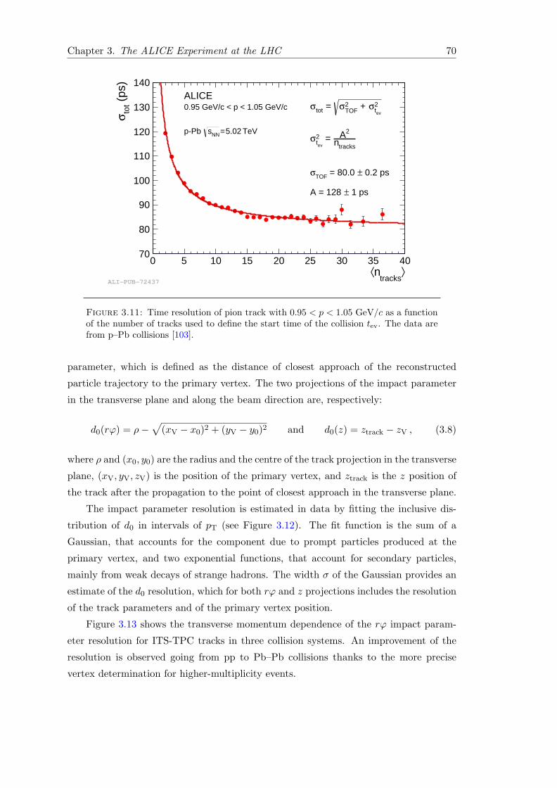
Chapter 3. The ALICE Experiment at the LHC 70
⟩tracks
n⟨0 5 10 15 20 25 30 35 40
(ps
)to
tσ
70
80
90
100
110
120
130
140ALICE0.95 GeV/c < p < 1.05 GeV/c
TeV 5.02 = NNspPb
2evtσ + 2
TOFσ = totσ
tracksn2A =
evt2σ
0.2 ps± = 80.0 TOFσ
1 ps±A = 128
ALI−PUB−72437
Figure 3.11: Time resolution of pion track with 0.95 < p < 1.05 GeV/c as a functionof the number of tracks used to define the start time of the collision tev. The data arefrom p–Pb collisions [103].
parameter, which is defined as the distance of closest approach of the reconstructed
particle trajectory to the primary vertex. The two projections of the impact parameter
in the transverse plane and along the beam direction are, respectively:
d0(rϕ) = ρ−√
(xV − x0)2 + (yV − y0)2 and d0(z) = ztrack − zV , (3.8)
where ρ and (x0, y0) are the radius and the centre of the track projection in the transverse
plane, (xV, yV, zV) is the position of the primary vertex, and ztrack is the z position of
the track after the propagation to the point of closest approach in the transverse plane.
The impact parameter resolution is estimated in data by fitting the inclusive dis-
tribution of d0 in intervals of pT (see Figure 3.12). The fit function is the sum of a
Gaussian, that accounts for the component due to prompt particles produced at the
primary vertex, and two exponential functions, that account for secondary particles,
mainly from weak decays of strange hadrons. The width σ of the Gaussian provides an
estimate of the d0 resolution, which for both rϕ and z projections includes the resolution
of the track parameters and of the primary vertex position.
Figure 3.13 shows the transverse momentum dependence of the rϕ impact param-
eter resolution for ITS-TPC tracks in three collision systems. An improvement of the
resolution is observed going from pp to Pb–Pb collisions thanks to the more precise
vertex determination for higher-multiplicity events.

Chapter 3. The ALICE Experiment at the LHC 71
m)µ (0,xy
d400 200 0 200 400
410
310
210
This thesis
= 5.02 TeVNN
spPb,
c=1.1 GeV/T
p
mµ0.1) ±=(68.6Gaus
σ
Figure 3.12: Fit to the distribution of the rϕ component of the impact parameterfor tracks of pT = 1.1 GeV/c in p–Pb collisions. The fit function (red) is the sum of aGaussian and two exponential funtions. The width of the Gaussian, which is indicated,represents the estimate of the d0 resolution at that pT.
(GeV/c)T
p110 1 10
m)
µ r
esol
utio
n (
0,xy
d
0
50
100
150
200
250
300
ALICEcharged particles
= 7 TeVspp
= 5.02 TeVNNspPb
= 2.76 TeVNNsPbPb
ALI−PUB−72263
Figure 3.13: Resolution of the rϕ projection of the impact parameter for ITS-TPCtracks. The contribution from the vertex resolution is included [103].


4Experimental Observables
This chapter introduces the experimental observables that were studied for this thesis.
The two quantities that were used to investigate the azimuthal anisotropy of the D0
production in semi-peripheral Pb–Pb collisions, namely the elliptic flow v2 and the nu-
clear modification factor azimuthal dependence, are defined in Section 4.1. Section 4.2 is
devoted to the definition of the observables that were measured to study the D0 produc-
tion in minimum-bias p–Pb collisions: the pT- and y-differential cross sections and the
nuclear modification factor RpPb. The observables used to investigate the dependence
of the D0 production on event activity are also defined.
The strategy to obtain the D0 proton–proton cross section at the proper energy,
which is used to compute the nuclear modification factor both in Pb–Pb and p–Pb
collisions, is described in the last part of the chapter (Section 4.3).
4.1 Azimuthal Anisotropy of D0 Production in Pb–
Pb Collisions
The azimuthal anisotropy of the D0 production was studied by measuring two observ-
ables: the elliptic flow v2 and the azimuthal dependence of the nuclear modification
factor RAA. Both measurements were performed for Pb–Pb collisions in the centrality
class 30-50%. The D0 v2 was measured also in the 0–10% and 10–30% centrality classes.
4.1.1 Event-Plane Definition
The basic quantity that is needed to study azimuthal anisotropy is the estimate of the
reaction-plane angle, which is defined by the vector of the impact parameter and the
beam direction. The reaction-plane angle can not be directly measured, but can be
estimated from the particle azimuthal distribution event-by-event. Anisotropic flow can
73

Chapter 4. Experimental Observables 74
fluctuate event to event, both in magnitude and direction even at fixed impact parameter.
One of the important sources of flow fluctuations are fluctuations in the initial geometry
of the overlapping region due to random nature of the interaction between constituents
of the two nuclei. The principal axis of the participant region can deviate from the
reaction plane inducing flow fluctuations [104].
The orientation of the reaction plane or, in case of flow fluctuations, the nth-
harmonic collision symmetry plane is estimated with the nth-harmonic event-plane angle,
ψn. For a given harmonic n, one constructs the two-dimensional event-plane vector Qn
from the measured azimuthal distribution of particles produced in the event as follows:
Qn = (Qn,x, Qn,y) =
(∑
i
wi cosnϕi,∑
i
wi sinnϕi,
). (4.1)
The sums run over all reconstructed tracks in the case of the TPC, or segments of
detectors with azimuthal segmentation like VZERO, FMD, ZDC, or PMD. The angle
ϕi is the azimuthal emission angle of the particle i or the azimuthal coordinate of the
detector element i, respectively. For TPC tracks the weight wi can be unity or a specific
function of pT. For segmented detectors, wi is the signal observed in the detector element
i. Using the components of the Q-vector one can calculate the ψn. The azimuthal angle
of the Q2-vector
ψ2 =1
2arctan 2(Q2,y, Q2,x) (4.2)
is an estimate of the second harmonic symmetry plane Ψ2 and it is used to determine
the second harmonic coefficient elliptic flow, v2.
The measured flow coefficients need to be corrected for the finite event-plane angle
resolution. The resolution correction factor is close to unity (zero) for perfect (poor)
reconstruction of the collision symmetry plane. The event-plane resolution for the second
harmonic is given by:
R2 = 〈cos[2(ψ2 −Ψ2)]〉 , (4.3)
where the angle brackets 〈〉 denote an average over a large event sample.
The resolution correction factor can be calculated using the two- or three-(sub-)
detector correlation technique. In case of two (sub-)detectors A and B the subevent
resolution is defined as
Rsub2 =
√〈cos[2(ψA2 − ψB2 )]〉 , (4.4)
where ψA2 and ψB2 are the event-plane angles of the two subevents, and the angle brackets
denote the average over an ensemble of the events.
In case of (sub-)detectors with different kinematic coverages, such as VZERO-A and
VZERO-C, a three-detector subevent technique can be used. In this case, the resolution

Chapter 4. Experimental Observables 75
for a given detector can be defined from the correlation between each detector pair
RA2 =
√〈cos[2(ψA2 − ψC2 )]〉〈cos[2(ψA2 − ψB2 )]〉
〈cos[2(ψB2 − ψC2 )]〉 , (4.5)
where ψA2 is the event-plane angle for which the resolution is calculated, and B and
C are any other two (sub-)detectors. One can get the resolution for each of the three
detectors by permutation of the event-plane angles. Variations in the event-plane res-
olution calculated with different methods indicate differences in their sensitivity to the
correlations unrelated to reaction plane (non-flow) and/or flow fluctuations.
4.1.2 Elliptic Flow
The D0 elliptic flow was measured with the event-plane method. The event-plane angle
ψ2 was determined event-by-event as explained in Section 4.1.1 and the D0 yields were
measured in two 90◦-wide orthogonal azimuthal regions:
1. in-plane, −π4 < ∆ϕ ≤ π
4 and 3π4 < ∆ϕ ≤ 5π
4 ,
2. out-of-plane, π4 < ∆ϕ ≤ 3π
4 and 5π4 < ∆ϕ ≤ 7π
4 ,
where ∆ϕ = ϕD−ψ2, with ϕD defined as the azimuthal angle of the D0 meson momentum
vector at the primary vertex. The v2 can be expressed in terms of the in-plane (Nin−plane)
and out-of-plane (Nout−of−plane) yields as:
v2{EP} =1
R2
π
4
Nin−plane −Nout−of−plane
Nin−plane +Nout−of−plane. (4.6)
This expression is obtained by integrating Equation (2.17) in the two azimuthal regions
and includes already the correction for the event-plane resolution 1/R2. The contribution
of higher harmonics to the v2 value calculated with this equation can be evaluated by
integrating the corresponding terms of the Fourier series. All the odd harmonics, as well
as v4 and v8, induce the same average contribution to Nin−plane and Nout−of−plane due
to symmetry, and therefore they do not affect v2 calculated with Equation (4.6). The
contribution of v6, v10 and higher harmonics was assumed to be negligible based on the
values measured for light-flavour hadrons [68, 105].
4.1.3 RAA Azimuthal Dependence
The azimuthal dependence of the nuclear modification factor was studied by measuring
the RAA of prompt1 D0 mesons in the in-plane and out-of-plane regions defined in
1Prompt D0 are the mesons coming directly from the fragmentation of the c quarks. The D0 whichresults from beauty meson decays are defined as ”feed-down D0”.

Chapter 4. Experimental Observables 76
Section 4.1.2. It is defined as:
Rin(out)AA (pT) =
2 · dN in(out)AA /dpT
〈TAA〉 · dσpp/dpT. (4.7)
dNin(out)AA /dpT are the D0 meson yields, integrated over the two 90◦-wide intervals used
to determine v2 with the event-plane method. The factor 2 in Equation (4.7) accounts
for the fact that the D meson yields for Pb–Pb collisions were integrated over half of the
full azimuth. The average value of the nuclear overlap function in the centrality class
30–50% is 〈TAA〉 = 3.87±0.18 mb−1 [16]. dσpp/dpT is the proton–proton reference cross
section, that will be described in Section 4.3.
The yields of prompt D0 mesons in the two azimuthal intervals were obtained as:
dND0
dpT
∣∣∣∣∣|y|<0.5
=1
∆y∆pT
fprompt(pT) · 12N
D0+D0
raw (pT)∣∣∣|y|<yfid
· crefl(pT)
(Acc× ε)prompt(pT) · BR ·Nevents. (4.8)
The raw yields ND0+D0
raw were divided by a factor of two to obtain the charge (particle
and antiparticle) averaged yields. The factor crefl(pT) was introduced to correct the
raw yields for the contribution of signal candidates that are counted both as a particle
(D0) and an antiparticle (D0) (see Section 5.5). To correct for the contribution of B
meson decay feed-down, the raw yields were multiplied by the prompt factor fprompt.
Furthermore, they were divided by the product of prompt D meson acceptance and
efficiency (Acc × ε)prompt, normalized by the decay channel branching ratio (BR), the
transverse momentum (∆pT) and rapidity (∆y = 2yfid) interval widths and the number
of events (Nevents). The normalization by ∆y gives the corrected yields in one unity of
rapidity |y| < 0.5.
The procedure applied to obtain the elements needed to compute the corrected yield
will be described in detail in Chapter 5.
4.2 D0 Production in p–Pb Collisions
The D0 production was studied in p–Pb collisions as a function of the transverse mo-
mentum and of the rapidity of the mesons. The pT-differential production cross section
was used to calculate the nuclear modification factor RpPb for prompt D0 mesons.
Furthermore, the multiplicity dependence of the D0 production was investigated
with two different analysis observables: the nuclear modification factor was measured in
different event-activity classes and the D0 invariant yields were studied as a function of
the charged-particle multiplicity.

Chapter 4. Experimental Observables 77
4.2.1 Production Cross Section and RpPb
The total cross section for hard processes σhardpA in proton–nucleus collisions can be
derived from the expression of the inelastic cross section of a pA collision σpA =∫
d2b[1− eσNN(s)TA(b)
]considering the first term of the expansion in orders of σhard
NN TA(b):
σhardpA ≈
∫d2bσhard
NN TA(b) , (4.9)
where σhardNN is the corresponding cross section in nucleon–nucleon collisions, and TA(b)
is the nuclear thickness function of the nucleus A at impact parameter b, normalized so
that∫
d2TA(b) = A [106]. Thus, integrating Equation (4.9) over impact parameter one
gets the minimum-bias cross section for a given hard process in pA collisions relative to
the same cross section in pp collisions:
(σhardpA )MB = A · σhard
NN . (4.10)
Therefore, the nuclear modification factor for prompt D mesons in minimum-bias
p–Pb collisions, RpPb, is given by:
RpPb =
(dσ
dpT
)pPb
A ·(
dσdpT
)pp
=
(dNdpT
)pPb
〈TpPb〉 ·(
dσdpT
)pp
. (4.11)
The D0 production cross section(
dσdpT
)pPb
was obtained as:
dσD0
dpT
∣∣∣∣∣|ylab|<0.5
=1
∆y∆pT
fprompt(pT) · 12 N
D0+D0
raw (pT)∣∣∣|ylab|<yfid
· crefl(pT)
(Acc× ε)prompt(pT) · BR · Lint. (4.12)
The integrated luminosity Lint was computed as NpPb,MB/σpPb,MB where NpPb,MB is the
number of p–Pb collisions passing the minimum-bias trigger condition and σpPb,MB is
the cross section of the minimum-bias trigger which was measured with the p–Pb van
der Meer scan and results 2.09 b± 3.7% (syst.) [107].
The pT- and y-differential cross section for prompt D0 was obtained by applying the
same formula used for the pT-differential cross section, Equation (4.12), but considering
the yield, the efficiency, and fprompt extracted in intervals of ylab.
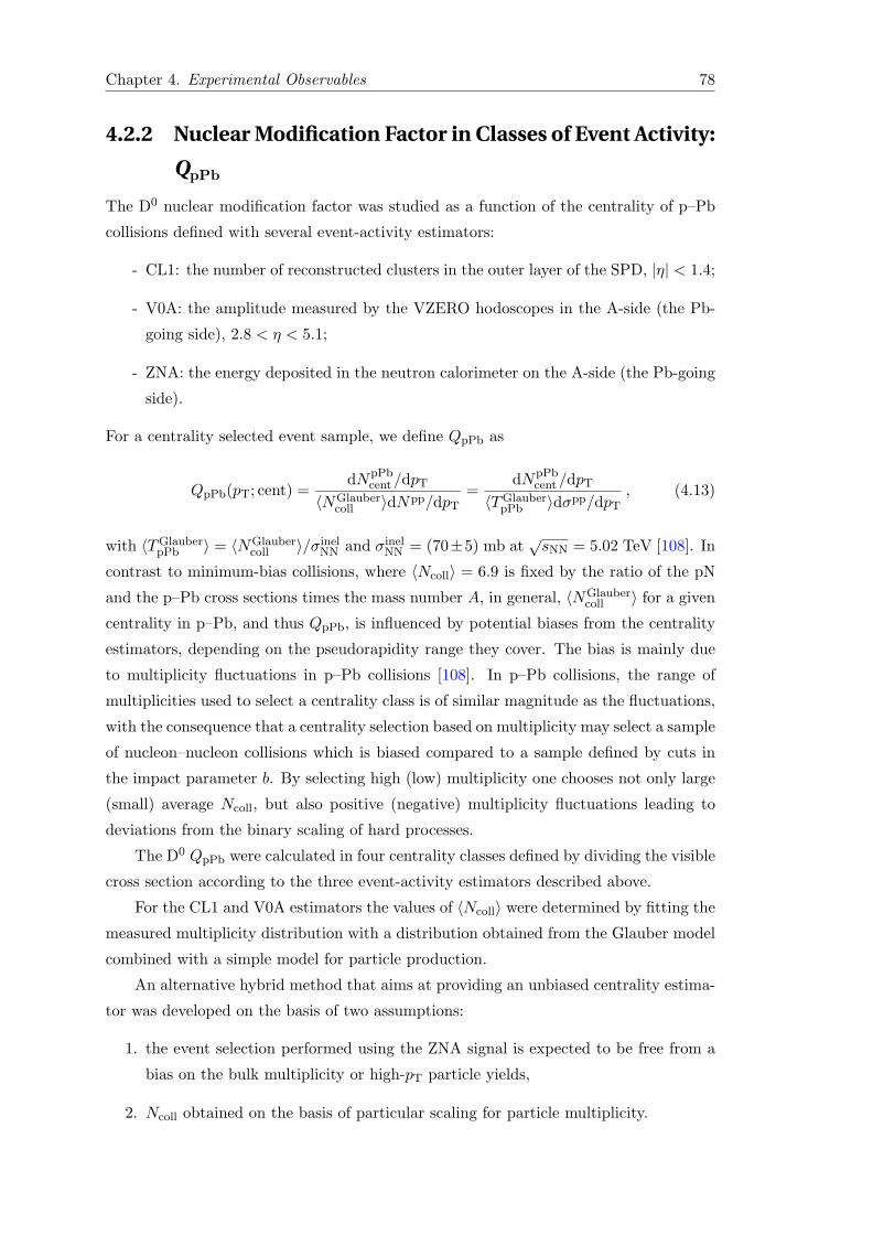
Chapter 4. Experimental Observables 78
4.2.2 Nuclear Modification Factor in Classes of Event Activity:
QpPb
The D0 nuclear modification factor was studied as a function of the centrality of p–Pb
collisions defined with several event-activity estimators:
- CL1: the number of reconstructed clusters in the outer layer of the SPD, |η| < 1.4;
- V0A: the amplitude measured by the VZERO hodoscopes in the A-side (the Pb-
going side), 2.8 < η < 5.1;
- ZNA: the energy deposited in the neutron calorimeter on the A-side (the Pb-going
side).
For a centrality selected event sample, we define QpPb as
QpPb(pT; cent) =dNpPb
cent/dpT
〈NGlaubercoll 〉dNpp/dpT
=dNpPb
cent/dpT
〈TGlauberpPb 〉dσpp/dpT
, (4.13)
with 〈TGlauberpPb 〉 = 〈NGlauber
coll 〉/σinelNN and σinel
NN = (70±5) mb at√sNN = 5.02 TeV [108]. In
contrast to minimum-bias collisions, where 〈Ncoll〉 = 6.9 is fixed by the ratio of the pN
and the p–Pb cross sections times the mass number A, in general, 〈NGlaubercoll 〉 for a given
centrality in p–Pb, and thus QpPb, is influenced by potential biases from the centrality
estimators, depending on the pseudorapidity range they cover. The bias is mainly due
to multiplicity fluctuations in p–Pb collisions [108]. In p–Pb collisions, the range of
multiplicities used to select a centrality class is of similar magnitude as the fluctuations,
with the consequence that a centrality selection based on multiplicity may select a sample
of nucleon–nucleon collisions which is biased compared to a sample defined by cuts in
the impact parameter b. By selecting high (low) multiplicity one chooses not only large
(small) average Ncoll, but also positive (negative) multiplicity fluctuations leading to
deviations from the binary scaling of hard processes.
The D0 QpPb were calculated in four centrality classes defined by dividing the visible
cross section according to the three event-activity estimators described above.
For the CL1 and V0A estimators the values of 〈Ncoll〉 were determined by fitting the
measured multiplicity distribution with a distribution obtained from the Glauber model
combined with a simple model for particle production.
An alternative hybrid method that aims at providing an unbiased centrality estima-
tor was developed on the basis of two assumptions:
1. the event selection performed using the ZNA signal is expected to be free from a
bias on the bulk multiplicity or high-pT particle yields,
2. Ncoll obtained on the basis of particular scaling for particle multiplicity.

Chapter 4. Experimental Observables 79
The centrality selection based on the energy measurement with the ZDC is expected to
introduce almost no bias on the binary scaling of hard processes owing to its large η-
separation from the central part of ALICE. One option to calculate 〈Ncoll〉 is to consider
that the charged-particle multiplicity at midrapidity is proportional to the number of
participants (Npart = Ncoll + 1) [109]. Therefore, the average number of binary NN
collisions in each centrality interval, was obtained by scaling the minimum-bias value of
〈Npart〉MB = 7.9 [110] accordingly to the multiplicity at midrapidity:
〈Npart〉multi = 〈Npart〉MB ·
( 〈dN/dη〉i〈dN/dη〉MB
)
−1<η<0
(4.14)
〈Ncoll〉multi = 〈Npart〉mult
i − 1 . (4.15)
The D0 QpPb calculated with the CL1 and V0A estimators and 〈TGlauberpPb 〉, as well
as with the hybrid method, will be presented in Chapter 8.
4.2.3 Self-normalized Yields
The second approach used to investigate the multiplicity dependence of the D0 pro-
duction in p–Pb collisions was the measurement of the D0 yield as a function of the
multiplicity of produced charged particles. The results will be given in Chapter 8 in
terms of the relative yields with respect to the yields in minimum-bias events:
(d2ND0/dydpT)j
〈d2ND0/dydpT〉=
(1
N jevent
N jraw D0
εjprompt D0
)/(1
NMB trigger/εMB trigger
〈Nraw D0〉〈εprompt D0〉
),
(4.16)
where the index j identifies the multiplicity interval, N jraw D0 are the raw yields for each
multiplicity and pT interval, εjprompt D0 the reconstruction and selection efficiencies and
N jevents the number of events analyzed in the considered multiplicity interval. Equa-
tion (4.16) holds under the assumption that the relative contribution to the D meson
raw yield due to the feed-down from B hadron decays does not depend on the multi-
plicity of the event, and is therefore canceling in the ratio to the multiplicity-integrated
values. The acceptance correction, defined as the fraction of D0 mesons within a given
rapidity and pT interval that decay into pairs of particles within the detector coverage,
cancels in this ratio. The number of events used for the normalization of the multiplicity
integrated yield has to be corrected for the fraction of inelastic events not seen by the
minimum-bias trigger condition, and it is therefore expressed as NMB trigger/εMB trigger,
with εMB trigger = (96.4± 2.2)%. It was verified with PYTHIA 6.4.21 Monte Carlo sim-
ulations that the minimum-bias trigger is 100% efficient for D mesons in the kinematic
range of the measurement meaning that the number of D0 in the minimum-bias triggered
events is the same as in the sample of inelastic events.

Chapter 4. Experimental Observables 80
The charged-particle multiplicity intervals were defined considering two alterna-
tive estimators. The first experimental estimator is the number of SPD tracklets in
|η| < 1.0, Ntracklets. As will be shown in Chapter 5, Monte Carlo simulations have
demonstrated that Ntracklets is proportional to the pseudorapidity density of the gener-
ated charged primary particles, dNch/dη. Primary particles are defined as prompt par-
ticles produced in the collision, including their decay products, except those from weak
decays of strange particles. The results obtained with the Ntracklets multiplicity estimator
are presented as a function of the relative charged-particle multiplicity at midrapidity,
(dNch/dη)j/〈dNch/dη〉, with 〈dNch/dη〉 = 17.64±0.01 (stat.)±0.15 (syst.) as measured
in inelastic p–Pb collisions producing at least one charged particle in |η| < 1 [109, 110].
The analysis of D0 production was also performed as a function of the charged-
particle multiplicity in the region 2.8 < η < 5.1, as measured with the charge col-
lected by the A side of the VZERO scintillator counters, NV0A, reported in units of the
minimum-ionizing-particle charge. The advantage of this estimator is that the event
multiplicity and the D meson yields are evaluated in different pseudorapidity ranges,
avoiding any possible auto-correlation. Monte Carlo simulations demonstrate that NV0A
is proportional to the charged-particle multiplicity in that pseudorapidity interval. The
D0 relative yields per event will be reported as a function of the relative uncorrected
multiplicity in the VZERO-A detector, NV0A/〈NV0A〉.
4.3 Proton–Proton Reference
The reference proton–proton cross section, which is needed to calculate the nuclear
modification factors in Pb–Pb and p–Pb collisions, was obtained by means of a pQCD-
based energy scaling of the pT-differential cross section measured at√s = 7 TeV [38].
The pT-dependent scaling factors were defined as the ratio of the cross sections obtained
from FONLL calculations [34–36] at√s = 2.76 TeV (or at
√s = 5.02 TeV) and 7 TeV.
The scaled D0 meson pT-differential cross section in 2 < pT < 16 GeV/c is consistent
with that measured at√s = 2.76 TeV using a smaller statistics data sample [39]. The
D0 cross section measured at 7 TeV in this pT range had smaller uncertainties with
respect to the measurement at 2.76 TeV and thus the scaled result from 7 TeV was used
as pp reference for the RAA(pA) calculation. The D0 cross section in pp collisions in the
interval 1 < pT < 2 GeV/c was measured at 7 and 2.76 TeV with similar uncertainty,
both results were scaled to 5.02 TeV, and averaged considering their relative statistical
uncertainties as weights.
The maximum pT reached by the current available ALICE pp measurement is limited
to pT = 16 GeV/c. To obtain the pp reference for the p–Pb measurements in the
16 < pT < 24 GeV/c interval, the measured pp cross section was extrapolated to
higher pT using the spectrum predicted by FONLL [34–36] scaled to match pp data in

Chapter 4. Experimental Observables 81
5 < pT < 16 GeV/c. Then the D0 cross section at 7 TeV in 16 < pT < 24 GeV/c was
scaled to 5.02 TeV.

5D0→ K−π+ Decay Reconstruction
The chapter is devoted to the description of the D0 analysis in Pb–Pb and p–Pb colli-
sions. The aim of the analysis is to extract the elements that are needed to measure the
elliptic flow in Pb–Pb collisions, the production cross section and nuclear modification
factor in both Pb–Pb and p–Pb collisions.
In the first part of the chapter, Section 5.1, the Pb–Pb and p–Pb data samples are
described. In Section 5.2 the event-plane determination for the azimuthal anisotropy
measurement is explained. Section 5.3 is devoted to the description of the reconstruc-
tion and selection strategy for D mesons. The strategy exploits the displacement (from
the primary vertex) of the secondary vertices originating from the weak decay of the D
mesons. The variables allowing to select the D0 → K−π+ topology will be introduced,
together with the particle identification procedure to improve the rejection of the com-
binatorial background. A description of the invariant mass analysis used to extract the
yields is given in Section 5.4. The invariant mass distributions together with the fits
performed to obtain the raw signals are shown for both Pb–Pb and p–Pb systems. Sec-
tion 5.5 describes the study of the D0 reflections, defined as the signal candidates that
pass the cuts both as D0 and D0. The last two sections, 5.6 and 5.7, are devoted to the
description of the efficiency calculation and feed-down correction, respectively.
5.1 Data Samples
Pb–Pb Collisions
The D0 azimuthal anisotropy analysis was performed on the data sample of Pb–Pb
collisions recorded in November and December 2011 at the centre-of-mass energy per
nucleon–nucleon collision of√sNN = 2.76 TeV. The events were collected with an in-
teraction trigger based on the information from the VZERO detector, which required
83
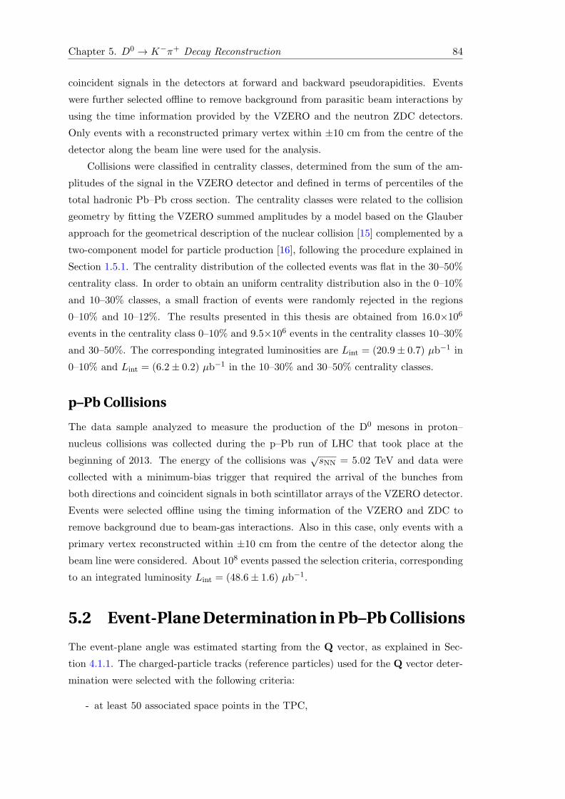
Chapter 5. D0 → K−π+ Decay Reconstruction 84
coincident signals in the detectors at forward and backward pseudorapidities. Events
were further selected offline to remove background from parasitic beam interactions by
using the time information provided by the VZERO and the neutron ZDC detectors.
Only events with a reconstructed primary vertex within ±10 cm from the centre of the
detector along the beam line were used for the analysis.
Collisions were classified in centrality classes, determined from the sum of the am-
plitudes of the signal in the VZERO detector and defined in terms of percentiles of the
total hadronic Pb–Pb cross section. The centrality classes were related to the collision
geometry by fitting the VZERO summed amplitudes by a model based on the Glauber
approach for the geometrical description of the nuclear collision [15] complemented by a
two-component model for particle production [16], following the procedure explained in
Section 1.5.1. The centrality distribution of the collected events was flat in the 30–50%
centrality class. In order to obtain an uniform centrality distribution also in the 0–10%
and 10–30% classes, a small fraction of events were randomly rejected in the regions
0–10% and 10–12%. The results presented in this thesis are obtained from 16.0×10⁶
events in the centrality class 0–10% and 9.5×10⁶ events in the centrality classes 10–30%
and 30–50%. The corresponding integrated luminosities are Lint = (20.9± 0.7) µb−1 in
0–10% and Lint = (6.2± 0.2) µb−1 in the 10–30% and 30–50% centrality classes.
p–Pb Collisions
The data sample analyzed to measure the production of the D0 mesons in proton–
nucleus collisions was collected during the p–Pb run of LHC that took place at the
beginning of 2013. The energy of the collisions was√sNN = 5.02 TeV and data were
collected with a minimum-bias trigger that required the arrival of the bunches from
both directions and coincident signals in both scintillator arrays of the VZERO detector.
Events were selected offline using the timing information of the VZERO and ZDC to
remove background due to beam-gas interactions. Also in this case, only events with a
primary vertex reconstructed within ±10 cm from the centre of the detector along the
beam line were considered. About 108 events passed the selection criteria, corresponding
to an integrated luminosity Lint = (48.6± 1.6) µb−1.
5.2 Event-Plane Determination in Pb–Pb Collisions
The event-plane angle was estimated starting from the Q vector, as explained in Sec-
tion 4.1.1. The charged-particle tracks (reference particles) used for the Q vector deter-
mination were selected with the following criteria:
- at least 50 associated space points in the TPC,

Chapter 5. D0 → K−π+ Decay Reconstruction 85
(rad)2
ψEvent plane angle 0 0.5 1 1.5 2 2.5 3
Nor
mal
ized
cou
nts
0.96
0.97
0.98
0.99
1
1.01
1.02
1.03
1.04 ALICE
=2.76 TeVNNsPbPb,
Centrality 3050%
< 0.8ηTPC, 0 <
)>=0.00122
ψ)>=0.0023, <sin(22
ψ<cos(2
VZERO
)>=0.00472
ψ)>=0.0012, <sin(22
ψ<cos(2
(a)
ALI−PUB−69887
(a)
Centrality (%)0 10 20 30 40 50 60 70
2R
0
0.1
0.2
0.3
0.4
0.5
0.6
0.7
0.8
0.9
1
< 0.8ηTPC, 0 <
VZERO
Syst from subevent definition
ALICE
=2.76 TeVNNsPbPb, (b)
ALI−PUB−69891
(b)
Figure 5.1: (a) Distribution of event-plane angle ψ2, estimated from TPC trackswith 0 < η < 0.8 (solid line) or with the VZERO detector signals (dashed line) in thecentrality range 30–50%. The distributions are normalized by their integral [111]. (b)Event-plane resolution correction factor R2 as a function of centrality for the TPC andVZERO detectors. The boxes represent the systematic uncertainties estimated fromthe variation of R2 when changing the subevents used for its determination [111].
- χ2/ndf < 2 for the momentum fit in the TPC,
- a distance of closest approach to the primary vertex smaller than 3.2 cm in z and
2.4 cm in the (x, y) plane,
- pT > 150 MeV/c.
The pseudorapidity interval was limited to the positive region 0 < η < 0.8, where
the TPC acceptance and efficiency were more uniform as a function of the azimuthal
angle for the analyzed data set. The remaining azimuthal non-uniformity was corrected
for using as weights wi in Equation (4.1) the inverse of the ϕ distribution of charged
particles used for the Q vector determination, 1/(dN/dϕi), multiplied by a function
f(pT) =
{pT/ GeV/c, pT < 2 GeV/c
2, pT ≥ 2 GeV/c. This function mimics the pT dependence of
the charged-particle v2 and it improves the estimate of Ψ2 by enhancing the contribution
of particles with a stronger flow signal. To avoid auto-correlations between the D meson
candidates and the event-plane angles, the Q vector was calculated for each candidate
excluding from the set of reference particles the tracks used to form that particular
candidate.
The distribution of the event-plane angle ψ2 obtained for this set of reference parti-
cles is shown in Figure 5.1(a), for the centrality range 30–50%. The distribution, divided
by its integral, exhibits a residual non-uniformity below 1% [111].
An additional study was performed with the Q vector determined from the az-
imuthal distribution of signals in the segments of the VZERO detectors, which are

Chapter 5. D0 → K−π+ Decay Reconstruction 86
sensitive to particles produced at forward and backward rapidities. Also with this
procedure the residual non-uniformity in the event-plane distribution is of about 1%
(Figure 5.1(a)) [111].
The event-plane resolution correction factor R2 was computed with the two- or
three-subevent methods for both strategies adopted to estimate the event-plane angle.
For the event plane computed using TPC tracks, R2 was determined from the correlation
of the event-plane angles reconstructed in the two sides of the TPC, −0.8 < η < 0 and
0 < η < 0.8, i.e. two samples of tracks with similar multiplicity and v2. R2 is shown in
Figure 5.1(b) as a function of collision centrality. The average R2 value in the centrality
class 30–50% is 0.8059 [111]. The statistical uncertainty is negligible (∼ 10−4). The
systematic uncertainty was estimated by using a three-subevent method considering the
event planes reconstructed in the TPC (0 < η < 0.8), VZERO-A (2.8 < η < 5.1) and
VZERO-C (−3.7 < η < −1.7).
The resolution of the event plane determined from the VZERO detector is also
shown in Figure 5.1(b). In this case, R2 was measured with three subevents, namely
the signal in the VZERO detector and the tracks in the positive and negative η region
of the TPC. The event-plane determination has a poorer resolution with the VZERO
detector than with the TPC tracks, thus, the v2 measurement is expected to be more
precise with the TPC event plane [111].
5.3 D0 Reconstruction and Selection
The reconstruction of charm mesons is performed with a common strategy within the
ALICE experiment. The lowest-mass charm hadron states, D0 and D+ (and antipar-
ticles), can decay only through weak processes and they have proper decay lengths of
a few hundred microns: cτ = 122.9 µm for the D0 and cτ = 311.8 µm for the D+ [7].
Therefore, the distance between the interaction point (primary vertex) and their decay
point (secondary vertex) is measurable. The D meson detection strategy is based on
an invariant mass analysis of fully reconstructed topologies originating from secondary
vertices.
The results presented in this thesis are based on the reconstruction and selection
of the D0 hadronic decay channel, D0 → K−π+ (D0 → K+π−), with branching ratio
B.R.= (3.88 ± 0.05)% [7]. A sketch of the decay is shown in Figure 5.2. The main
feature of this topology is the presence of two tracks displaced from the primary vertex
and originating from a common point.

Chapter 5. D0 → K−π+ Decay Reconstruction 87
1784 ALICE Collaboration
πpointing angle θpointing
secondary vertexprimary vertex
D reconstructed momentum 0
D flight line0
d
d
0
0
K
K
π
impact parameters ~100 mµ
Figure 6.278. Schematic representation of the D0 ! K�⇡+ decay with the impact parameters(d0) and the pointing angle (✓pointing).
6.6.4. Charm reconstruction in the D0 ! K�⇡+ channel. The feasibility study for thereconstruction of D0 mesons in the K�⇡+ decay channel in central Pb–Pb collisions [53,834] is presented in detail in Sections 6.6.4.1– 6.6.4.4. The same study was repeated also forthe case of pp [53] and pPb collisions [835]; the aspects which are specific to these cases andthe results are reported in Sections 6.6.4.5 and 6.6.4.6. The extrapolated results for differentvalues of the magnetic field in the ALICE barrel are reported in Section 6.6.4.7. Statistical andsystematic uncertainties on the measurement of the D0 production cross section are discussedin Section 6.6.4.8.
6.6.4.1. Detection strategy. The lowest-mass charm hadron states, D0 and D+ (andantiparticles), can decay only through weak processes and they have proper decay lengthsof few hundred microns (c⌧ = (123.0 ± 0.4) µm for the D0 and c⌧ = (311.8 ± 2.1) µm forthe D+ [409]). Therefore, the distance between the interaction point (primary vertex) and theirdecay point (secondary vertex) is measurable. The selection of a suitable decay channel, whichinvolves only charged-particle products, allows the direct identification of the charm states bycomputing the invariant mass of fully reconstructed topologies originating from secondaryvertices.
In this analysis we follow the general lines for the detection strategy of open charm in thehadronic channels defined in the ALICE ITS Technical Design Report [1]. We consider as a
benchmark the process D0 ! K�⇡+ (and D0 ! K+⇡� ); the branching ratio for this channel
is (3.83 ± 0.09)% [409]. Colour Figure V shows the event display picture of a D0 ! K�⇡+
decay in the ALICE Silicon Pixel Detector.A sketch of the decay is shown in Fig. 6.278. The main feature of this topology is the
presence of two tracks displaced from the primary vertex and compatible with originatingfrom a common point. The variable that allows one to evaluate the displacement of a track isthe impact parameter, defined as the distance of closest approach of the track to the primaryvertex. We indicate as d0 the projection of the impact parameter on the bending plane (r'),normal to the field, and beam, direction. The decay products of D0 mesons have typical r'
impact parameters ranging from about 50 µm, for pD0
t ' 0.5 GeV/c, to about 120 µm, forpD0
t > 5 GeV/c.The impact parameter resolution depends mainly on the thickness and radius of the beam-
pipe and on the position, spatial resolution, and material thickness of the inner detector layers.In ALICE, the beam-pipe, built in beryllium, has a thickness of 0.8 mm (0.3% of X0) and
Figure 5.2: Schematic representation of the D0 → K−π+ decay with the impact pa-rameters (d0) and the pointing angle (θpointing).
5.3.1 Secondary Vertex Reconstruction
The knowledge of the momenta of the decay tracks and of the position of the secondary
vertex allows the complete reconstruction of the momentum of the particle that has
decayed.
The secondary vertex is reconstructed for a given pair of opposite-sign tracks by a
minimization of the distance in space between the two helices representing the tracks.
Once the minimum segment between the tracks is found, the position of the vertex on
this segment is defined keeping into account the different spatial precisions of the two
tracks, which are estimated by the track covariance matrix. The track with the largest
momentum has better precision (see Figure 3.13) and, therefore, the vertex is usually
estimated to be closer to this track than to the lower-momentum one.
The resolution on the secondary vertex position is strongly correlated to the impact
parameter resolution: it is better in the bending plane (x and y) than along z and, for
pT < 2–3 GeV/c, it improves as pT increases. At low pT, the decay tracks are affected
by multiple scattering and the resolution deteriorates, while at high pT the worsening
is due to the fact that the angle between the decay tracks becomes smaller as the pT of
the D0 increases and, thus, the determination of the crossing point becomes less precise.
For intermediate pT (∼ 2 GeV/c) the resolution is of about 70 µm [112].
5.3.2 Topological Selection Strategy
The reconstructed tracks are grouped in pairs following the charge ordering of the de-
cay channel, defining the D0 candidates. For each candidate the secondary vertex is
computed, and the candidates are selected on the basis of typical kinematical and geo-
metrical properties that characterize the single tracks and the reconstructed secondary
vertex. The high tracking spatial precision provided by the ITS detector allows to recon-
struct the primary vertex position with high precision and, then, to tag displaced tracks
with distances to the interaction point of few tens of microns. In order to select signal

Chapter 5. D0 → K−π+ Decay Reconstruction 88118 D0 ! K�⇡+ reconstrunction in Pb–Pb collisions
a common point, like a decay vertex or the primary vertex of interaction (ideal dca=0),the observed dca is determined by the detector spatial resolution on the track position.In Fig. 2, left panel, the dca distributions for background (from the pp minimum-biassample) and signal (from the charm enriched sample) pairs are shown.
m]µdca [0 100 200 300 400 500 600 700 800 900 10000
0.01
0.02
0.03
0.04
0.05
0.06Background
Signal
*θcos −1 −0.8 −0.6 −0.4 −0.2 0 0.2 0.4 0.6 0.8 1
0.01
0.015
0.02
0.025
0.03
0.035
0.04Background
Signal
Figure 2: Distance of closest approach dca (left panel) and cos �⇤ (right panel) distributionsfor background and signal candidates. The variables are defined in the text.
pointingθcos 0 0.1 0.2 0.3 0.4 0.5 0.6 0.7 0.8 0.9 10
0.02
0.04
0.06
0.08
0.1
0.12
0.14
0.16
0.18
0.2
0.22
0.24
Background
Signal
]2mµ [π0xdK
0d−100 −80 −60 −40 −20 0 20 40 60 80 100
310×−510
−410
−310
−210
−110
Background
Signal
Figure 3: cos �pointing (left) and product of impact parameters dK0 ⇥ d⇡0 (right) distribu-tions for background and signal candidates. The variables are defined in the text. A cutcos �pointing > 0 was applied already at the level of candidates reconstruction.
The D0 decay angle �⇤ is defined as the angle between the kaon momentum in theD0 rest frame and the boost direction. For each candidate, two values are calculated, onefor each mass hypothesis (the D0 [D0] hypothesis implies the negative [positive] trackto be interpreted as the kaon). As shown in Fig. 2 (right panel), due to the isotropicdecay direction in the D0 rest frame, the cos �⇤ distribution for signal pairs (reflectionsare rejected here) is essentially flat. Conversely, the background distribution peaks closeto ±1. The depletion at | cos �⇤| ⇡ 1 is related to the cuts applied in the candidatereconstruction (track pt > 0.3 GeV/c) and to detector e�ects: if the particles are emittedparallel to the D0 momentum, one of the two is boosted at very low momenta and cango out of the geometrical acceptance. Due to the di�erent masses of the two D0 decay
4
Figure 5.4: Distance of closest approach of signal (red) and background (blue) D0 candi-dates obtained with a pp PYTHIA Monte Carlo (left). Distribution of the cosine of the ✓⇤
angle for signal and background candidates(right). For signal the distribution is flat dueto the isotropic emission with respect to the c.m.s of the D0.
Tracks are first selected using quality selections on the track reconstruction in thedetector. These quality cuts are related to:
- the number of clusters the track has in the TPC (Ncl > 70),
- the track acceptance (|⌘| < 0.8),
- the quality of the fit in the Kalman filter procedure (�2/dof < 2).
Tracks should have at least one point in one of the two layers of the SPD, in order toreject secondaries.
The single track cuts applied are on the impact parameter with respect to the primaryvertex and on the single track transverse momentum. As already shown in Sec. 3.10,the impact parameter resolution in Pb–Pb collisions is about 50 µm for tracks with pt ⇠1 GeV/c. A minimum cut on the impact parameter of the tracks reduces the numberof primary tracks, while a maximum cut can reject those with large displacement, likestrange or beauty hadrons decays and particles coming from photon conversions in thedetector material. For low pt D0 the main contribution to the impact parameter comesfrom the detector resolution, more than the real c⌧ of the D0, due to multiple scatteringe↵ects.
The distance of closest approach (dca) between two tracks is the length of a segmentminimizing the distance between the two tracks trajectories. If two tracks come from thesame point the ideal dca should be zero. The measured dca is determined by detectorresolution on the track position.
Most of the background is made of primary tracks: their dca distribution is stronglycorrelated with the impact parameter resolution. The dca cut is e↵ective in rejecting thebackground pairs if a cut on the minimum impact parameter is applied (Fig. 5.4 left).
In the D0 reference system, the pion and the kaon are emitted isotropically with threemomenta of equal magnitude and opposite direction. The ✓⇤ angle is computed in twodi↵erent mass hypotesis (D0 and D0) to correlate both charged tracks with the possibilityof being a kaon. Due to the isotropic production in the c.m.s, the cos ✓⇤ distribution forsignal pairs is almost flat. The background distribution peaks close to ±1. For | cos ✓⇤| ⇠ 1
(a)
118 D0 ! K�⇡+ reconstrunction in Pb–Pb collisions
a common point, like a decay vertex or the primary vertex of interaction (ideal dca=0),the observed dca is determined by the detector spatial resolution on the track position.In Fig. 2, left panel, the dca distributions for background (from the pp minimum-biassample) and signal (from the charm enriched sample) pairs are shown.
m]µdca [0 100 200 300 400 500 600 700 800 900 10000
0.01
0.02
0.03
0.04
0.05
0.06Background
Signal
*θcos −1 −0.8 −0.6 −0.4 −0.2 0 0.2 0.4 0.6 0.8 1
0.01
0.015
0.02
0.025
0.03
0.035
0.04Background
Signal
Figure 2: Distance of closest approach dca (left panel) and cos �⇤ (right panel) distributionsfor background and signal candidates. The variables are defined in the text.
pointingθcos 0 0.1 0.2 0.3 0.4 0.5 0.6 0.7 0.8 0.9 10
0.02
0.04
0.06
0.08
0.1
0.12
0.14
0.16
0.18
0.2
0.22
0.24
Background
Signal
]2mµ [π0xdK
0d−100 −80 −60 −40 −20 0 20 40 60 80 100
310×−510
−410
−310
−210
−110
Background
Signal
Figure 3: cos �pointing (left) and product of impact parameters dK0 ⇥ d⇡0 (right) distribu-tions for background and signal candidates. The variables are defined in the text. A cutcos �pointing > 0 was applied already at the level of candidates reconstruction.
The D0 decay angle �⇤ is defined as the angle between the kaon momentum in theD0 rest frame and the boost direction. For each candidate, two values are calculated, onefor each mass hypothesis (the D0 [D0] hypothesis implies the negative [positive] trackto be interpreted as the kaon). As shown in Fig. 2 (right panel), due to the isotropicdecay direction in the D0 rest frame, the cos �⇤ distribution for signal pairs (reflectionsare rejected here) is essentially flat. Conversely, the background distribution peaks closeto ±1. The depletion at | cos �⇤| ⇡ 1 is related to the cuts applied in the candidatereconstruction (track pt > 0.3 GeV/c) and to detector e�ects: if the particles are emittedparallel to the D0 momentum, one of the two is boosted at very low momenta and cango out of the geometrical acceptance. Due to the di�erent masses of the two D0 decay
4
Figure 5.4: Distance of closest approach of signal (red) and background (blue) D0 candi-dates obtained with a pp PYTHIA Monte Carlo (left). Distribution of the cosine of the ✓⇤
angle for signal and background candidates(right). For signal the distribution is flat dueto the isotropic emission with respect to the c.m.s of the D0.
Tracks are first selected using quality selections on the track reconstruction in thedetector. These quality cuts are related to:
- the number of clusters the track has in the TPC (Ncl > 70),
- the track acceptance (|⌘| < 0.8),
- the quality of the fit in the Kalman filter procedure (�2/dof < 2).
Tracks should have at least one point in one of the two layers of the SPD, in order toreject secondaries.
The single track cuts applied are on the impact parameter with respect to the primaryvertex and on the single track transverse momentum. As already shown in Sec. 3.10,the impact parameter resolution in Pb–Pb collisions is about 50 µm for tracks with pt ⇠1 GeV/c. A minimum cut on the impact parameter of the tracks reduces the numberof primary tracks, while a maximum cut can reject those with large displacement, likestrange or beauty hadrons decays and particles coming from photon conversions in thedetector material. For low pt D0 the main contribution to the impact parameter comesfrom the detector resolution, more than the real c⌧ of the D0, due to multiple scatteringe↵ects.
The distance of closest approach (dca) between two tracks is the length of a segmentminimizing the distance between the two tracks trajectories. If two tracks come from thesame point the ideal dca should be zero. The measured dca is determined by detectorresolution on the track position.
Most of the background is made of primary tracks: their dca distribution is stronglycorrelated with the impact parameter resolution. The dca cut is e↵ective in rejecting thebackground pairs if a cut on the minimum impact parameter is applied (Fig. 5.4 left).
In the D0 reference system, the pion and the kaon are emitted isotropically with threemomenta of equal magnitude and opposite direction. The ✓⇤ angle is computed in twodi↵erent mass hypotesis (D0 and D0) to correlate both charged tracks with the possibilityof being a kaon. Due to the isotropic production in the c.m.s, the cos ✓⇤ distribution forsignal pairs is almost flat. The background distribution peaks close to ±1. For | cos ✓⇤| ⇠ 1
(b)
Figure 5.3: (a) Distance of closest approach (dca) of signal (red) and background(black) D0 candidates obtained with a pp PYTHIA simulation. (b) Distribution of theθ∗ angle for signal and background candidates. For signal the distribution is almost flatdue to the isotropic emission of the pion and the kaon in the centre-of-mass system.
candidates among the huge number of those obtained by combinatorial association, the
key point is to measure the separation between the primary and the secondary vertices.
Several variables are used to reject background candidates and to select as much
signal as possible. The variables used to enhance the signal-to-background ratio can be
subdivided into two classes: single track variables and candidate variables.
The track selection criteria are:
- pseudorapidity within the TPC fiducial acceptance (|η| < 0.8),
- the number of space points in the TPC (Ncl > 70),
- the quality of the momentum fit in the TPC (χ2/ndf < 2),
- at least one hit in either of the two layers of the SPD (helps in rejecting secon-
daries).
The selection of tracks with |η| < 0.8 introduces a steep drop in the acceptance of
D mesons for rapidities larger than 0.7–0.8, depending on pT. A D meson fiducial
acceptance region was, therefore, defined as |y| < yfid(pT), with yfid(pT) increasing from
0.5 to 0.8 in 0 < pT < 5 GeV/c and taking a constant value of 0.8 for pT > 5 GeV/c.
Cuts are applied on the impact parameter (the projection on the transverse plane
d0(rϕ)) with respect to the primary vertex and on the track transverse momentum. The
impact parameter resolution in Pb–Pb and p–Pb collisions is about 60 µm and 70 µm,
respectively, for tracks with pT = 1 GeV/c, as shown is Section 3.5. A lower limit on the
impact parameter of the tracks reduces the number of primary tracks, while an upper
cut allows to reject those with large displacement, e.g. from strange-hadron decays and
electrons coming from photon conversions in the detector material.
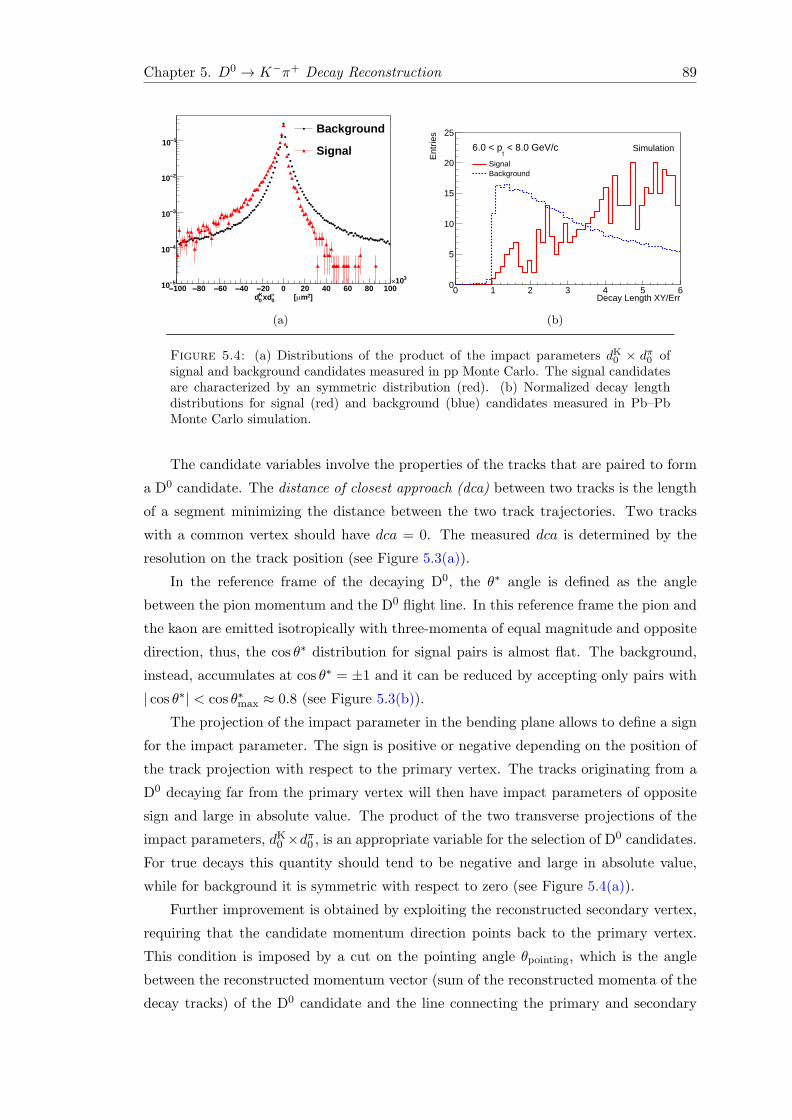
Chapter 5. D0 → K−π+ Decay Reconstruction 89120 D0 ! K�⇡+ reconstrunction in Pb–Pb collisions
a common point, like a decay vertex or the primary vertex of interaction (ideal dca=0),the observed dca is determined by the detector spatial resolution on the track position.In Fig. 2, left panel, the dca distributions for background (from the pp minimum-biassample) and signal (from the charm enriched sample) pairs are shown.
m]µdca [0 100 200 300 400 500 600 700 800 900 10000
0.01
0.02
0.03
0.04
0.05
0.06Background
Signal
*θcos −1 −0.8 −0.6 −0.4 −0.2 0 0.2 0.4 0.6 0.8 1
0.01
0.015
0.02
0.025
0.03
0.035
0.04Background
Signal
Figure 2: Distance of closest approach dca (left panel) and cos �⇤ (right panel) distributionsfor background and signal candidates. The variables are defined in the text.
pointingθcos 0 0.1 0.2 0.3 0.4 0.5 0.6 0.7 0.8 0.9 10
0.02
0.04
0.06
0.08
0.1
0.12
0.14
0.16
0.18
0.2
0.22
0.24
Background
Signal
]2mµ [π0xdK
0d−100 −80 −60 −40 −20 0 20 40 60 80 100
310×−510
−410
−310
−210
−110
Background
Signal
Figure 3: cos �pointing (left) and product of impact parameters dK0 ⇥ d⇡0 (right) distribu-tions for background and signal candidates. The variables are defined in the text. A cutcos �pointing > 0 was applied already at the level of candidates reconstruction.
The D0 decay angle �⇤ is defined as the angle between the kaon momentum in theD0 rest frame and the boost direction. For each candidate, two values are calculated, onefor each mass hypothesis (the D0 [D0] hypothesis implies the negative [positive] trackto be interpreted as the kaon). As shown in Fig. 2 (right panel), due to the isotropicdecay direction in the D0 rest frame, the cos �⇤ distribution for signal pairs (reflectionsare rejected here) is essentially flat. Conversely, the background distribution peaks closeto ±1. The depletion at | cos �⇤| ⇡ 1 is related to the cuts applied in the candidatereconstruction (track pt > 0.3 GeV/c) and to detector e�ects: if the particles are emittedparallel to the D0 momentum, one of the two is boosted at very low momenta and cango out of the geometrical acceptance. Due to the di�erent masses of the two D0 decay
4
Decay Length XY/Err0 1 2 3 4 5 6
Ent
ries
0
5
10
15
20
25
< 8.0 GeV/ct
6.0 < p
SignalBackground
Simulation
Figure 5.6: Products of the impact parameter of signal and background candidates mea-sured in pp Monte Carlo. The asymmetric distribution is typical of signal candidates (left).Normalized decay length distributions for signal and background candidates measured inPb–Pb Monte Carlo simulation (right).
For D0 with pt < 3 GeV/c, an additional selection has been applied in order to rejectthe combinatorial background. Both tracks of the D0 candidate must have a hit in theinner layer of the SPD detector. This selection reduces the signal by a factor proportionalto the dead zones of this layer (⇠ 15%) but it reduces the background by a factor 2.
The values used as selection cuts were chosen in order to reject as much background aspossibile without losing too much signal. The adopted criterion is to try to maximize thestatistical significance, checking that the invariant mass position and width are compatiblewith the Particle Data Group (PDG) ones [145].
The statistical significance is defined as
S =Sp
S +B=
pS
1q1 + 1
r
, (5.2)
with S and B the signal background candidates after cuts and r = S/B the signal-to-background ratio, that depends on the “power” of the cuts. The significance describeshow much the signal emerges above the fluctuations of the background.
For the Pb–Pb analysis the most e�cient cuts are the cosine of the pointing angle inthe xy plane and the normalized decay length, in addition to the products of the impactparameters. In Tables 5.2 and 5.3 the values of the selection cuts, described previouslyand used for the analysis in Pb–Pb collisions are reported. Di↵erent selection cuts havebeen used in central events events and peripheral ones, due to the di↵erent amount ofbackground in the events of the two centrality classes. For peripheral events the selectioncuts are looser, since the background is smaller. With the selection cuts shown in thetables, other cuts are applied for both centrality classes and for all pt ranges:
- the di↵erence between the mass of the reconstructed candidates and the PDG D0
mass has to be smaller than 0.4 GeV,
- | cos ✓⇤| < 0.8,
- the pt of the two charged tracks has to be larger than 0.7 GeV/c, 1
1This cut is di↵erent for D0 with pt < 2 GeV/c
(a)
120 D0 ! K�⇡+ reconstrunction in Pb–Pb collisions
a common point, like a decay vertex or the primary vertex of interaction (ideal dca=0),the observed dca is determined by the detector spatial resolution on the track position.In Fig. 2, left panel, the dca distributions for background (from the pp minimum-biassample) and signal (from the charm enriched sample) pairs are shown.
m]µdca [0 100 200 300 400 500 600 700 800 900 10000
0.01
0.02
0.03
0.04
0.05
0.06Background
Signal
*θcos −1 −0.8 −0.6 −0.4 −0.2 0 0.2 0.4 0.6 0.8 1
0.01
0.015
0.02
0.025
0.03
0.035
0.04Background
Signal
Figure 2: Distance of closest approach dca (left panel) and cos �⇤ (right panel) distributionsfor background and signal candidates. The variables are defined in the text.
pointingθcos 0 0.1 0.2 0.3 0.4 0.5 0.6 0.7 0.8 0.9 10
0.02
0.04
0.06
0.08
0.1
0.12
0.14
0.16
0.18
0.2
0.22
0.24
Background
Signal
]2mµ [π0xdK
0d−100 −80 −60 −40 −20 0 20 40 60 80 100
310×−510
−410
−310
−210
−110
Background
Signal
Figure 3: cos �pointing (left) and product of impact parameters dK0 ⇥ d⇡0 (right) distribu-tions for background and signal candidates. The variables are defined in the text. A cutcos �pointing > 0 was applied already at the level of candidates reconstruction.
The D0 decay angle �⇤ is defined as the angle between the kaon momentum in theD0 rest frame and the boost direction. For each candidate, two values are calculated, onefor each mass hypothesis (the D0 [D0] hypothesis implies the negative [positive] trackto be interpreted as the kaon). As shown in Fig. 2 (right panel), due to the isotropicdecay direction in the D0 rest frame, the cos �⇤ distribution for signal pairs (reflectionsare rejected here) is essentially flat. Conversely, the background distribution peaks closeto ±1. The depletion at | cos �⇤| ⇡ 1 is related to the cuts applied in the candidatereconstruction (track pt > 0.3 GeV/c) and to detector e�ects: if the particles are emittedparallel to the D0 momentum, one of the two is boosted at very low momenta and cango out of the geometrical acceptance. Due to the di�erent masses of the two D0 decay
4
Decay Length XY/Err0 1 2 3 4 5 6
Ent
ries
0
5
10
15
20
25
< 8.0 GeV/ct
6.0 < p
SignalBackground
Simulation
Figure 5.6: Products of the impact parameter of signal and background candidates mea-sured in pp Monte Carlo. The asymmetric distribution is typical of signal candidates (left).Normalized decay length distributions for signal and background candidates measured inPb–Pb Monte Carlo simulation (right).
For D0 with pt < 3 GeV/c, an additional selection has been applied in order to rejectthe combinatorial background. Both tracks of the D0 candidate must have a hit in theinner layer of the SPD detector. This selection reduces the signal by a factor proportionalto the dead zones of this layer (⇠ 15%) but it reduces the background by a factor 2.
The values used as selection cuts were chosen in order to reject as much background aspossibile without losing too much signal. The adopted criterion is to try to maximize thestatistical significance, checking that the invariant mass position and width are compatiblewith the Particle Data Group (PDG) ones [145].
The statistical significance is defined as
S =Sp
S +B=
pS
1q1 + 1
r
, (5.2)
with S and B the signal background candidates after cuts and r = S/B the signal-to-background ratio, that depends on the “power” of the cuts. The significance describeshow much the signal emerges above the fluctuations of the background.
For the Pb–Pb analysis the most e�cient cuts are the cosine of the pointing angle inthe xy plane and the normalized decay length, in addition to the products of the impactparameters. In Tables 5.2 and 5.3 the values of the selection cuts, described previouslyand used for the analysis in Pb–Pb collisions are reported. Di↵erent selection cuts havebeen used in central events events and peripheral ones, due to the di↵erent amount ofbackground in the events of the two centrality classes. For peripheral events the selectioncuts are looser, since the background is smaller. With the selection cuts shown in thetables, other cuts are applied for both centrality classes and for all pt ranges:
- the di↵erence between the mass of the reconstructed candidates and the PDG D0
mass has to be smaller than 0.4 GeV,
- | cos ✓⇤| < 0.8,
- the pt of the two charged tracks has to be larger than 0.7 GeV/c, 1
1This cut is di↵erent for D0 with pt < 2 GeV/c
(b)
Figure 5.4: (a) Distributions of the product of the impact parameters dK0 × dπ0 of
signal and background candidates measured in pp Monte Carlo. The signal candidatesare characterized by an symmetric distribution (red). (b) Normalized decay lengthdistributions for signal (red) and background (blue) candidates measured in Pb–PbMonte Carlo simulation.
The candidate variables involve the properties of the tracks that are paired to form
a D0 candidate. The distance of closest approach (dca) between two tracks is the length
of a segment minimizing the distance between the two track trajectories. Two tracks
with a common vertex should have dca = 0. The measured dca is determined by the
resolution on the track position (see Figure 5.3(a)).
In the reference frame of the decaying D0, the θ∗ angle is defined as the angle
between the pion momentum and the D0 flight line. In this reference frame the pion and
the kaon are emitted isotropically with three-momenta of equal magnitude and opposite
direction, thus, the cos θ∗ distribution for signal pairs is almost flat. The background,
instead, accumulates at cos θ∗ = ±1 and it can be reduced by accepting only pairs with
| cos θ∗| < cos θ∗max ≈ 0.8 (see Figure 5.3(b)).
The projection of the impact parameter in the bending plane allows to define a sign
for the impact parameter. The sign is positive or negative depending on the position of
the track projection with respect to the primary vertex. The tracks originating from a
D0 decaying far from the primary vertex will then have impact parameters of opposite
sign and large in absolute value. The product of the two transverse projections of the
impact parameters, dK0 ×dπ0 , is an appropriate variable for the selection of D0 candidates.
For true decays this quantity should tend to be negative and large in absolute value,
while for background it is symmetric with respect to zero (see Figure 5.4(a)).
Further improvement is obtained by exploiting the reconstructed secondary vertex,
requiring that the candidate momentum direction points back to the primary vertex.
This condition is imposed by a cut on the pointing angle θpointing, which is the angle
between the reconstructed momentum vector (sum of the reconstructed momenta of the
decay tracks) of the D0 candidate and the line connecting the primary and secondary

Chapter 5. D0 → K−π+ Decay Reconstruction 90
5.2 D0 in Pb–Pb collisions 119
a drop of the number of candidates is visible, due to the cuts applied in the reconstructionand to detector acceptance e↵ects (Fig. 5.4 right).
Pointθcos0 0.1 0.2 0.3 0.4 0.5 0.6 0.7 0.8 0.9 1
Ent
ries
0
100
200
300
400
500
600
700
< 3.0 GeV/ct
2.0 < p
SignalBackground
Simulation
pointingXYθcos0.7 0.75 0.8 0.85 0.9 0.95 1
Ent
ries
0
100
200
300
400
500
600
700
800
900
1000
< 3.0 GeV/ct
2.0 < p
SignalBackground
Simulation
Figure 5.5: Distribution of the cosine of the pointing angle for signal and backgroundcandidates measured in Pb–Pb Monte Carlo (left). Distribution of the cosine of the point-ing angle measured in the transverse plane with respect to the beam line for signal andbackground candidates measured in a HIJING charm enriched Monte Carlo (right)
The pointing angle (✓point) has been already introduced in the previous section and inFig. 5.2. For background pairs there is no correlation between the reconstructed momen-tum and the reconstructed flight line, since the secondary vertex is an artifact of the finitetracking resolution. For a signal candidate the flight line direction is determined by theD0 three-momentum direction and the cosine of the pointing angle distribution is peakedat 1. The comparison between Monte Carlo distributions of signal and background areshown in Fig. 5.5 (left).
The pointing angle can be defined with respect the full reference frame of the decayor also considering only the transverse plane (defined as xy plane). In this plane asshown in Sect. 4.3 the size of the luminous region is much smaller with respect to the zcoordinate. The primary vertex resolution is thus better in the xy plane. Considering thepointing angle defined in the transverse plane, it is then possible to introduce a new cutvariable that allows to better separate background candidates with respect to the signalones. This variable (✓point XY) was used only in the Pb–Pb analysis, to cope with thelarger background. The comparison between signal and background is shown in Fig. 5.5(right). The distribution for the cos ✓point XY is more “peaked” close to 1 with respect tothe pointing angle 3D, especially for the signal candidates.
The product of impact parameters (d0 K ⇥ d0 ⇡) is built considering the single trackimpact parameters and the charge of the tracks: for a signal candidate, the product wouldbe negative. Due to detector resolution, the distribution of the signal shows both positiveand negative sides but it is asymmetric with respect to zero. For background candidates,composed of randomly associated primary tracks with opposite charges, the distributionis symmetric (Fig. 5.6 left).
Another important variable used only in the Pb–Pb analysis is the normalized decaylength measured in the transverse plane (LXY ). The decay length in the transverse planewith respect to the beam line is divided (normalized) by the error on the decay lengthmeasurement. As Fig. 5.6 (right) shows, background dominates at small normalized decaylengths. In case of a charm or beauty decay, the particles are displaced and the measure-ment of decay length is more precise. At low pt (pt < 2 GeV/c) the decay length startssu↵ering also from detector resolution e↵ects and also for signal candidates it can be lessprecise. In that case the selection cut needs to be released.
(a)
5.2 D0 in Pb–Pb collisions 119
a drop of the number of candidates is visible, due to the cuts applied in the reconstructionand to detector acceptance e↵ects (Fig. 5.4 right).
Pointθcos0 0.1 0.2 0.3 0.4 0.5 0.6 0.7 0.8 0.9 1
Ent
ries
0
100
200
300
400
500
600
700
< 3.0 GeV/ct
2.0 < p
SignalBackground
Simulation
pointingXYθcos0.7 0.75 0.8 0.85 0.9 0.95 1
Ent
ries
0
100
200
300
400
500
600
700
800
900
1000
< 3.0 GeV/ct
2.0 < p
SignalBackground
Simulation
Figure 5.5: Distribution of the cosine of the pointing angle for signal and backgroundcandidates measured in Pb–Pb Monte Carlo (left). Distribution of the cosine of the point-ing angle measured in the transverse plane with respect to the beam line for signal andbackground candidates measured in a HIJING charm enriched Monte Carlo (right)
The pointing angle (✓point) has been already introduced in the previous section and inFig. 5.2. For background pairs there is no correlation between the reconstructed momen-tum and the reconstructed flight line, since the secondary vertex is an artifact of the finitetracking resolution. For a signal candidate the flight line direction is determined by theD0 three-momentum direction and the cosine of the pointing angle distribution is peakedat 1. The comparison between Monte Carlo distributions of signal and background areshown in Fig. 5.5 (left).
The pointing angle can be defined with respect the full reference frame of the decayor also considering only the transverse plane (defined as xy plane). In this plane asshown in Sect. 4.3 the size of the luminous region is much smaller with respect to the zcoordinate. The primary vertex resolution is thus better in the xy plane. Considering thepointing angle defined in the transverse plane, it is then possible to introduce a new cutvariable that allows to better separate background candidates with respect to the signalones. This variable (✓point XY) was used only in the Pb–Pb analysis, to cope with thelarger background. The comparison between signal and background is shown in Fig. 5.5(right). The distribution for the cos ✓point XY is more “peaked” close to 1 with respect tothe pointing angle 3D, especially for the signal candidates.
The product of impact parameters (d0 K ⇥ d0 ⇡) is built considering the single trackimpact parameters and the charge of the tracks: for a signal candidate, the product wouldbe negative. Due to detector resolution, the distribution of the signal shows both positiveand negative sides but it is asymmetric with respect to zero. For background candidates,composed of randomly associated primary tracks with opposite charges, the distributionis symmetric (Fig. 5.6 left).
Another important variable used only in the Pb–Pb analysis is the normalized decaylength measured in the transverse plane (LXY ). The decay length in the transverse planewith respect to the beam line is divided (normalized) by the error on the decay lengthmeasurement. As Fig. 5.6 (right) shows, background dominates at small normalized decaylengths. In case of a charm or beauty decay, the particles are displaced and the measure-ment of decay length is more precise. At low pt (pt < 2 GeV/c) the decay length startssu↵ering also from detector resolution e↵ects and also for signal candidates it can be lessprecise. In that case the selection cut needs to be released.
(b)
Figure 5.5: (a) Distribution of the cosine of the pointing angle cos θpointing for signal(red) and background (blue) candidates in Pb–Pb Monte Carlo. (b) Distribution of thecosine of the pointing angle measured in the transverse plane cos θxypointing for signal andbackground candidates measured in a HIJING charm enriched Monte Carlo.
vertex (D0 flight line). For background pairs there is no correlation between the recon-
structed momentum and the reconstructed flight line, so that the cos θpointing is almost
uniformly distributed. The signal, instead, is characterized by a distribution peaked at
+1 (see Figure 5.5(a)).
The pointing angle can be defined in 3D space, or also considering only the transverse
plane, where the tracking and the primary vertex resolutions are better. A new cut
variable can, thus, be introduced to better separate background candidates with respect
to signal ones. The distribution of the cos θxypointing is more peaked close to 1 with respect
to the pointing angle in three dimensions, and is used in the Pb–Pb analysis to cope
with the larger background (see Figure 5.5(b)).
The last selection variable, used only in the Pb–Pb analysis, is the normalized decay
length in the transverse plane Lxy. It is obtained by dividing (normalizing) the decay
length (distance between the reconstructed primary and secondary vertex) in the trans-
verse plane by the uncertainty on its measurement. The background is characterized by
small normalized decay length, as can be seen in Figure 5.4(b).
The values used as selection cuts were chosen in order to reject as much background
as possible without losing too much signal, and, in general for Pb–Pb analysis the cuts
are tighter with respect to p–Pb due to the larger combinatorial background. The
values of the selection cuts applied in Pb–Pb and p–Pb are reported in the next section
(Section 5.4).
5.3.3 Particle Identification
For the D0 analysis, the Particle Identification (PID) is mainly used to identify the
kaon in the candidate and remove the high combinatorial background from pairs of

Chapter 5. D0 → K−π+ Decay Reconstruction 91
pions. Kaons (and pions) are identified via the specific energy loss (dE/dx) in the TPC
(Section 3.4.1) and the time of flight measurements in the TOF (Section 3.4.2). These
two detectors can separate kaons and pions from other particles in different momentum
ranges. With both detectors a track can be identified on the basis of the difference,
expressed in units of resolution (σ), between the measured signal and that expected for
the considered particle species (nσ cut method). For the D0, the PID selection is aimed
at reducing the background while preserving most of the signal.
The same PID strategy was applied for Pb–Pb and p–Pb analysis.
In order to assign the kaon or pion mass to the decay tracks, compatibility cuts were
applied to the difference between the measured and the expected TPC and TOF signals.
For both dE/dx and time of flight, a 3σ compatibility cut was used for all momenta
(a track is not excluded as a pion or kaon in the TPC (TOF) if its signal is within
3σ from the expected dE/dx (time of flight) for the pion or kaon hypothesis). Tracks
without a TOF signal were identified using only the TPC information, and tracks with
incompatible TOF and TPC indications were considered to be compatible with both
pion and kaon.
In the TPC, a 2σ cut was applied to identify both pions and kaons. If the track
energy loss signal is between 2 and 3σ from the expected value, the track is used both
as pion and kaon. In the momentum interval 0.6 < p < 0.8 GeV/c, the selection band
is tightened to 1σ, since the pion and kaon expectations become closer.
If the track reaches the TOF, a 3σ cut is applied on its expected arrival time.
Kaons are identified up to p = 2 GeV/c, and for larger momenta, particles are used
both as pion and kaon since the signal bands of pions and kaons start to overlap and
the contamination effect is not negligible anymore.
Two-prong candidates were accepted (as D0, D0, or both) or rejected on the basis of
their compatibility with the K∓π± final state. If a true D0 candidate is compatible with
both D0 and D0 hypotheses, the “wrong” one, which can not be rejected on a candidate
by candidate basis, is called “reflection” (Section 5.5).
5.4 Yield Extraction
The D0 raw yields were extracted in several pT intervals from an invariant mass analysis
of the candidates that pass the topological cuts and the PID requirements. For each
D0 candidate the invariant mass is calculated as M(Kπ) =√
(EK + Eπ)2 − (~pK + ~pπ)2
starting from the reconstructed information of the corresponding pair of tracks. The
K±π∓ invariant mass distribution can be considered as the sum of a Gaussian function
representing the D0 signal and the background, that is described with an exponential
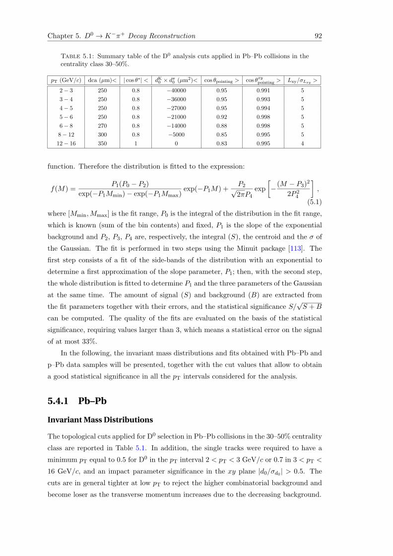
Chapter 5. D0 → K−π+ Decay Reconstruction 92
Table 5.1: Summary table of the D0 analysis cuts applied in Pb–Pb collisions in thecentrality class 30–50%.
pT (GeV/c) dca (µm)< | cos θ∗| < dK0 × dπ0 (µm2)< cos θpointing > cos θxypointing > Lxy/σLxy >
2− 3 250 0.8 −40000 0.95 0.991 5
3− 4 250 0.8 −36000 0.95 0.993 5
4− 5 250 0.8 −27000 0.95 0.994 5
5− 6 250 0.8 −21000 0.92 0.998 5
6− 8 270 0.8 −14000 0.88 0.998 5
8− 12 300 0.8 −5000 0.85 0.995 5
12− 16 350 1 0 0.83 0.995 4
function. Therefore the distribution is fitted to the expression:
f(M) =P1(P0 − P2)
exp(−P1Mmin)− exp(−P1Mmax)exp(−P1M) +
P2√2πP4
exp
[−(M − P3)2
2P 24
],
(5.1)
where [Mmin,Mmax] is the fit range, P0 is the integral of the distribution in the fit range,
which is known (sum of the bin contents) and fixed, P1 is the slope of the exponential
background and P2, P3, P4 are, respectively, the integral (S), the centroid and the σ of
the Gaussian. The fit is performed in two steps using the Minuit package [113]. The
first step consists of a fit of the side-bands of the distribution with an exponential to
determine a first approximation of the slope parameter, P1; then, with the second step,
the whole distribution is fitted to determine P1 and the three parameters of the Gaussian
at the same time. The amount of signal (S) and background (B) are extracted from
the fit parameters together with their errors, and the statistical significance S/√S +B
can be computed. The quality of the fits are evaluated on the basis of the statistical
significance, requiring values larger than 3, which means a statistical error on the signal
of at most 33%.
In the following, the invariant mass distributions and fits obtained with Pb–Pb and
p–Pb data samples will be presented, together with the cut values that allow to obtain
a good statistical significance in all the pT intervals considered for the analysis.
5.4.1 Pb–Pb
Invariant Mass Distributions
The topological cuts applied for D0 selection in Pb–Pb collisions in the 30–50% centrality
class are reported in Table 5.1. In addition, the single tracks were required to have a
minimum pT equal to 0.5 for D0 in the pT interval 2 < pT < 3 GeV/c or 0.7 in 3 < pT <
16 GeV/c, and an impact parameter significance in the xy plane |d0/σd0 | > 0.5. The
cuts are in general tighter at low pT to reject the higher combinatorial background and
become loser as the transverse momentum increases due to the decreasing background.

Chapter 5. D0 → K−π+ Decay Reconstruction 93
)2
c) (GeV/π(KM
1.7 1.75 1.8 1.85 1.9 1.95 2 2.05
2 cE
ntrie
s / 1
2 M
eV/
0
200
400
600
800
1000 c<3 GeV/T
p2<
+π
K→
0Dand charge conj.
InPlane
OutofPlane
)2
c) (GeV/π(KM
1.7 1.75 1.8 1.85 1.9 1.95 2
2 cE
ntrie
s / 1
5 M
eV/
0
50
100
150
200
250
300
350
400
450 c<4 GeV/T
p3<
PbPb, 3050%=2.76 TeV
NNs
)2
c) (GeV/π(KM
1.7 1.75 1.8 1.85 1.9 1.95 2
2 cE
ntrie
s / 1
5 M
eV/
0
50
100
150
200
250
300 c<6 GeV/T
p4<ALICE
)2
c) (GeV/π(KM
1.7 1.75 1.8 1.85 1.9 1.95 2
2 cE
ntrie
s / 1
5 M
eV/
0
10
20
30
40
50
60
70
80
c<8 GeV/T
p6<
)2
c) (GeV/π(KM
1.7 1.75 1.8 1.85 1.9 1.95 2 2.05
2 cE
ntrie
s / 2
3 M
eV/
0
10
20
30
40
50
60
70
80
90
100
c<12 GeV/T
p8<
)2
c) (GeV/π(KM
1.7 1.75 1.8 1.85 1.9 1.95 2 2.05
2 cE
ntrie
s / 3
1 M
eV/
0
5
10
15
20
25
30
35
40
45
50
c<16 GeV/T
p12<
Figure 5.6: Distributions of the invariant mass for D0 in the two ∆ϕ intervals, forPb–Pb collisions in the 30–50% centrality class [111].
Table 5.2: Summary table of the D0 raw yield (S) and significance extracted in eachpT interval in-plane and out-of-plane in Pb–Pb collisions in the centrality class 30–50%.
pT (GeV/c)S Significance
In-plane Out-of-plane In-plane Out-of-plane
2− 3 739± 66 526± 55 11.2 9.6
3− 4 452± 36 297± 28 12.5 10.6
4− 6 429± 33 276± 25 13 11
6− 8 150± 18 115± 15 8.3 7.7
8− 12 195± 19 77± 14 10.3 5.5
12− 16 56± 13 76± 11 4.3 6.9
The D0 meson yield was extracted in the in-plane and the out-of-plane regions de-
fined in Section 4.1.2. The invariant mass distributions for the D0 meson are shown in
Figure 5.6 in six pT intervals for the 30–50% centrality class, along with the fits used for
the yield estimation [111]. The raw signal, background and significance extracted in each
pT interval are reported in Table 5.2. When fitting the invariant mass distribution in
the two ∆ϕ intervals, the centroid and the width of the Gaussian functions were fixed to
those obtained from a fit to the invariant mass distribution integrated over ϕ, where the
statistical significance of the signal is larger. The centroids for the ϕ-integrated distri-
butions were found to be in agreement with the D0 meson world-average [7] mass value
and with the values from the simulation, confirming that the background fluctuations
were not causing a distortion in the signal line shape.
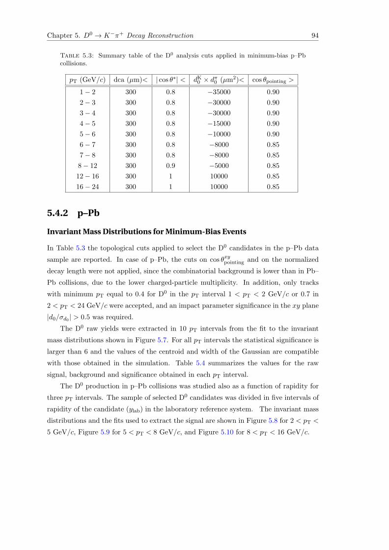
Chapter 5. D0 → K−π+ Decay Reconstruction 94
Table 5.3: Summary table of the D0 analysis cuts applied in minimum-bias p–Pbcollisions.
pT (GeV/c) dca (µm)< | cos θ∗| < dK0 × dπ0 (µm2)< cos θpointing >
1− 2 300 0.8 −35000 0.90
2− 3 300 0.8 −30000 0.90
3− 4 300 0.8 −30000 0.90
4− 5 300 0.8 −15000 0.90
5− 6 300 0.8 −10000 0.90
6− 7 300 0.8 −8000 0.85
7− 8 300 0.8 −8000 0.85
8− 12 300 0.9 −5000 0.85
12− 16 300 1 10000 0.85
16− 24 300 1 10000 0.85
5.4.2 p–Pb
Invariant Mass Distributions for Minimum-Bias Events
In Table 5.3 the topological cuts applied to select the D0 candidates in the p–Pb data
sample are reported. In case of p–Pb, the cuts on cos θxypointing and on the normalized
decay length were not applied, since the combinatorial background is lower than in Pb–
Pb collisions, due to the lower charged-particle multiplicity. In addition, only tracks
with minimum pT equal to 0.4 for D0 in the pT interval 1 < pT < 2 GeV/c or 0.7 in
2 < pT < 24 GeV/c were accepted, and an impact parameter significance in the xy plane
|d0/σd0 | > 0.5 was required.
The D0 raw yields were extracted in 10 pT intervals from the fit to the invariant
mass distributions shown in Figure 5.7. For all pT intervals the statistical significance is
larger than 6 and the values of the centroid and width of the Gaussian are compatible
with those obtained in the simulation. Table 5.4 summarizes the values for the raw
signal, background and significance obtained in each pT interval.
The D0 production in p–Pb collisions was studied also as a function of rapidity for
three pT intervals. The sample of selected D0 candidates was divided in five intervals of
rapidity of the candidate (ylab) in the laboratory reference system. The invariant mass
distributions and the fits used to extract the signal are shown in Figure 5.8 for 2 < pT <
5 GeV/c, Figure 5.9 for 5 < pT < 8 GeV/c, and Figure 5.10 for 8 < pT < 16 GeV/c.
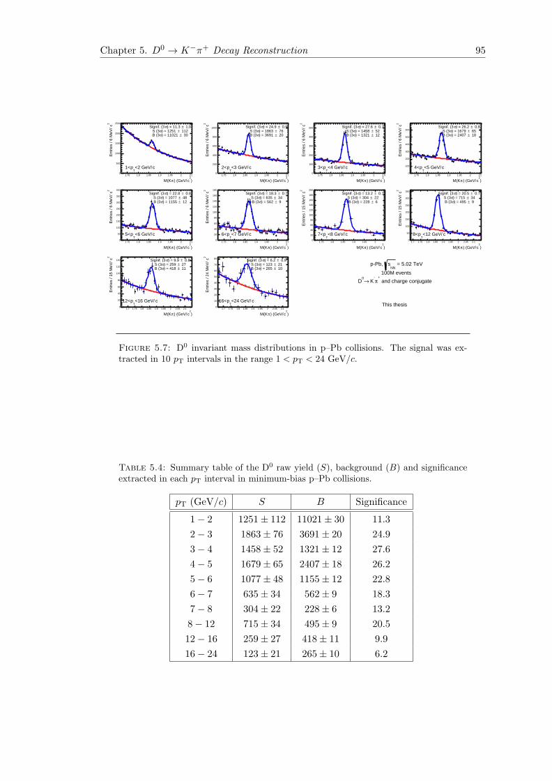
Chapter 5. D0 → K−π+ Decay Reconstruction 95
= 5.02 TeVNN
spPb,
100M events
and charge conjugate+
π
K→0
D
This thesis
)2
c) (GeV/π(KM
1.75 1.8 1.85 1.9 1.95 2 2.05
2 cE
ntrie
s / 6
MeV
/
0
500
1000
1500
2000
2500
c<2 GeV/T
p1<
1.0±) = 11.3 σSignif. (3 112±) = 1251 σS (3 30±) = 11021 σB (3
)2
c) (GeV/π(KM
1.75 1.8 1.85 1.9 1.95 2 2.05
2 cE
ntrie
s / 6
MeV
/
0
200
400
600
800
1000
c<3 GeV/T
p2<
0.9±) = 24.9 σSignif. (3 76±) = 1863 σS (3 20±) = 3691 σB (3
)2
c) (GeV/π(KM
1.75 1.8 1.85 1.9 1.95 2 2.05
2 cE
ntrie
s / 6
MeV
/
0
100
200
300
400
500
c<4 GeV/T
p3<
0.7±) = 27.6 σSignif. (3 52±) = 1458 σS (3 12±) = 1321 σB (3
)2
c) (GeV/π(KM
1.75 1.8 1.85 1.9 1.95 2 2.05
2 cE
ntrie
s / 6
MeV
/
0
100
200
300
400
500
600
c<5 GeV/T
p4<
0.8±) = 26.2 σSignif. (3 65±) = 1679 σS (3 18±) = 2407 σB (3
)2
c) (GeV/π(KM
1.75 1.8 1.85 1.9 1.95 2 2.05
2 cE
ntrie
s / 6
MeV
/
0
50
100
150
200
250
300
350
400
c<6 GeV/T
p5<
0.8±) = 22.8 σSignif. (3 48±) = 1077 σS (3 12±) = 1155 σB (3
)2
c) (GeV/π(KM
1.75 1.8 1.85 1.9 1.95 2 2.05
2 cE
ntrie
s / 6
MeV
/
0
20
40
60
80
100
120
140
160
180
c<7 GeV/T
p6<
0.7±) = 18.3 σSignif. (3 34±) = 635 σS (3 9±) = 562 σB (3
)2
c) (GeV/π(KM
1.75 1.8 1.85 1.9 1.95 2
2 cE
ntrie
s / 1
5 M
eV/
0
20
40
60
80
100
120
140
160
180
200
c<8 GeV/T
p7<
0.7±) = 13.2 σSignif. (3 22±) = 304 σS (3 6±) = 228 σB (3
)2
c) (GeV/π(KM
1.7 1.75 1.8 1.85 1.9 1.95 2 2.05 2.1
2 cE
ntrie
s / 1
5 M
eV/
0
50
100
150
200
250
300
350
c<12 GeV/T
p8<
0.7±) = 20.5 σSignif. (3 34±) = 715 σS (3 9±) = 495 σB (3
)2
c) (GeV/π(KM
1.7 1.75 1.8 1.85 1.9 1.95 2 2.05 2.1
2 cE
ntrie
s / 1
5 M
eV/
0
20
40
60
80
100
120
140
c<16 GeV/T
p12<
0.8±) = 9.9 σSignif. (3 27±) = 259 σS (3 11±) = 418 σB (3
)2
c) (GeV/π(KM
1.7 1.75 1.8 1.85 1.9 1.95 2 2.05 2.1
2 cE
ntrie
s / 2
4 M
eV/
0
10
20
30
40
50
60
70
80
c<24 GeV/T
p16<
0.9±) = 6.2 σSignif. (3 21±) = 123 σS (3 10±) = 265 σB (3
Figure 5.7: D0 invariant mass distributions in p–Pb collisions. The signal was ex-tracted in 10 pT intervals in the range 1 < pT < 24 GeV/c.
Table 5.4: Summary table of the D0 raw yield (S), background (B) and significanceextracted in each pT interval in minimum-bias p–Pb collisions.
pT (GeV/c) S B Significance
1− 2 1251± 112 11021± 30 11.3
2− 3 1863± 76 3691± 20 24.9
3− 4 1458± 52 1321± 12 27.6
4− 5 1679± 65 2407± 18 26.2
5− 6 1077± 48 1155± 12 22.8
6− 7 635± 34 562± 9 18.3
7− 8 304± 22 228± 6 13.2
8− 12 715± 34 495± 9 20.5
12− 16 259± 27 418± 11 9.9
16− 24 123± 21 265± 10 6.2
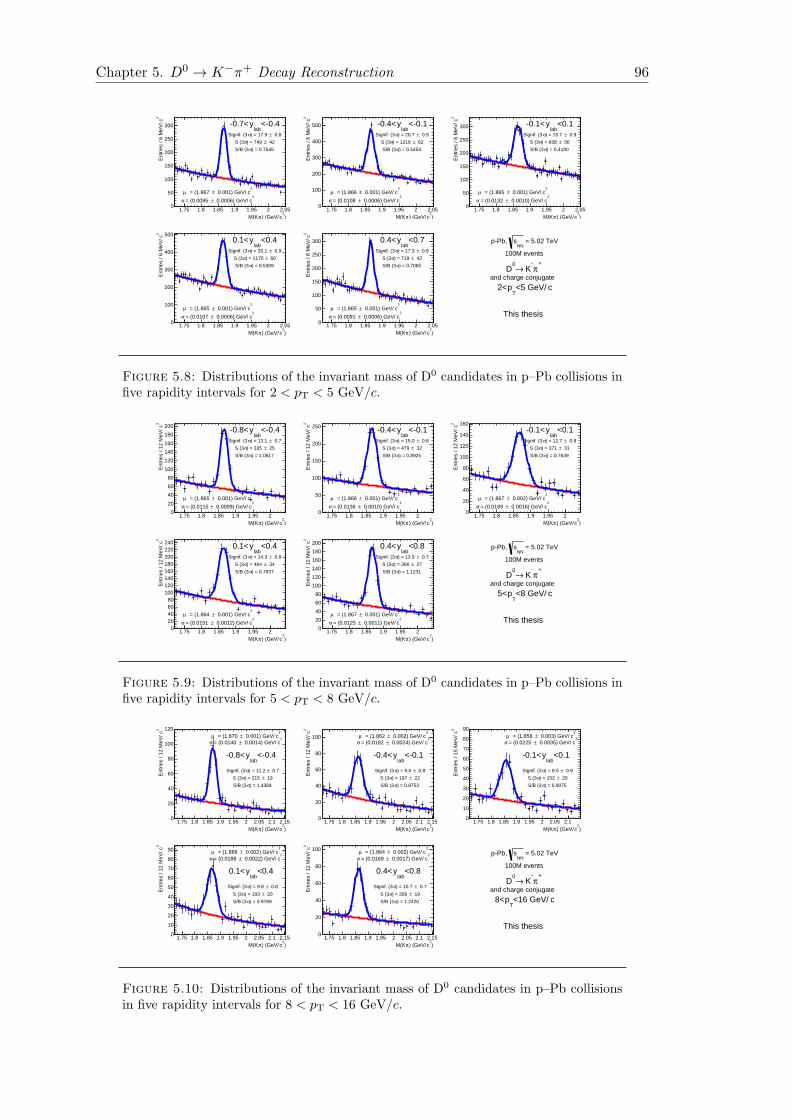
Chapter 5. D0 → K−π+ Decay Reconstruction 96
)2
c) (GeV/π(KM1.75 1.8 1.85 1.9 1.95 2 2.05
2 cE
ntrie
s / 6
MeV
/
0
50
100
150
200
250
300
2c 0.001) GeV/± = (1.867 µ
2c 0.0006) GeV/± = (0.0095 σ
0.8±) = 17.9 σSignif. (3
42±) = 749 σS (3
) = 0.7545σS/B (3
<0.4lab
y0.7<
)2
c) (GeV/π(KM1.75 1.8 1.85 1.9 1.95 2 2.05
2 cE
ntrie
s / 6
MeV
/
0
100
200
300
400
500
2c 0.001) GeV/± = (1.866 µ
2c 0.0006) GeV/± = (0.0108 σ
0.9±) = 20.7 σSignif. (3
62±) = 1219 σS (3
) = 0.5454σS/B (3
<0.1lab
y0.4<
)2
c) (GeV/π(KM1.75 1.8 1.85 1.9 1.95 2 2.05
2 cE
ntrie
s / 6
MeV
/
0
50
100
150
200
250
300
2c 0.001) GeV/± = (1.865 µ
2c 0.0010) GeV/± = (0.0132 σ
0.9±) = 15.7 σSignif. (3
56±) = 838 σS (3
) = 0.4180σS/B (3
<0.1lab
y0.1<
)2
c) (GeV/π(KM1.75 1.8 1.85 1.9 1.95 2 2.05
2 cE
ntrie
s / 6
MeV
/
0
100
200
300
400
500
2c 0.001) GeV/± = (1.865 µ
2c 0.0006) GeV/± = (0.0107 σ
0.9±) = 20.1 σSignif. (3
60±) = 1170 σS (3
) = 0.5309σS/B (3
<0.4lab
y0.1<
)2
c) (GeV/π(KM1.75 1.8 1.85 1.9 1.95 2 2.05
2 cE
ntrie
s / 6
MeV
/
0
50
100
150
200
250
300
2c 0.001) GeV/± = (1.865 µ
2c 0.0006) GeV/± = (0.0091 σ
0.8±) = 17.3 σSignif. (3
42±) = 719 σS (3
) = 0.7065σS/B (3
<0.7lab
y0.4< = 5.02 TeVNN
spPb,
100M events
and charge conjugate
+π
K→
0D
c<5 GeV/T
p2<
This thesis
Figure 5.8: Distributions of the invariant mass of D0 candidates in p–Pb collisions infive rapidity intervals for 2 < pT < 5 GeV/c.
)2
c) (GeV/π(KM1.75 1.8 1.85 1.9 1.95 2
2 cE
ntrie
s / 1
2 M
eV/
0
20
40
60
80
100
120
140
160
180
200
2c 0.001) GeV/± = (1.865 µ
2c 0.0009) GeV/± = (0.0115 σ
0.7±) = 13.1 σSignif. (3
25±) = 335 σS (3
) = 1.0617σS/B (3
<0.4lab
y0.8<
)2
c) (GeV/π(KM1.75 1.8 1.85 1.9 1.95 2
2 cE
ntrie
s / 1
2 M
eV/
0
50
100
150
200
250
2c 0.001) GeV/± = (1.866 µ
2c 0.0010) GeV/± = (0.0136 σ
0.8±) = 15.0 σSignif. (3
32±) = 479 σS (3
) = 0.8925σS/B (3
<0.1lab
y0.4<
)2
c) (GeV/π(KM1.75 1.8 1.85 1.9 1.95 2
2 cE
ntrie
s / 1
2 M
eV/
0
20
40
60
80
100
120
140
160
2c 0.002) GeV/± = (1.867 µ
2c 0.0016) GeV/± = (0.0189 σ
0.8±) = 12.7 σSignif. (3
31±) = 371 σS (3
) = 0.7639σS/B (3
<0.1lab
y0.1<
)2
c) (GeV/π(KM1.75 1.8 1.85 1.9 1.95 2
2 cE
ntrie
s / 1
2 M
eV/
020406080
100120140160180200220240
2c 0.001) GeV/± = (1.864 µ
2c 0.0012) GeV/± = (0.0151 σ
0.8±) = 14.3 σSignif. (3
34±) = 464 σS (3
) = 0.7837σS/B (3
<0.4lab
y0.1<
)2
c) (GeV/π(KM1.75 1.8 1.85 1.9 1.95 2
2 cE
ntrie
s / 1
2 M
eV/
0
20
40
60
80
100
120
140
160
180
200
2c 0.001) GeV/± = (1.867 µ
2c 0.0011) GeV/± = (0.0125 σ
0.7±) = 13.9 σSignif. (3
27±) = 366 σS (3
) = 1.1231σS/B (3
<0.8lab
y0.4< = 5.02 TeVNN
spPb,
100M events
and charge conjugate
+π
K→
0D
c<8 GeV/T
p5<
This thesis
Figure 5.9: Distributions of the invariant mass of D0 candidates in p–Pb collisions infive rapidity intervals for 5 < pT < 8 GeV/c.
)2
c) (GeV/π(KM1.75 1.8 1.85 1.9 1.95 2 2.05 2.1 2.15
2 cE
ntrie
s / 1
2 M
eV/
0
20
40
60
80
100
1202
c 0.001) GeV/± = (1.870 µ2
c 0.0014) GeV/± = (0.0140 σ
0.7±) = 11.2 σSignif. (3
19±) = 215 σS (3
) = 1.4384σS/B (3
<0.4lab
y0.8<
)2
c) (GeV/π(KM1.75 1.8 1.85 1.9 1.95 2 2.05 2.1 2.15
2 cE
ntrie
s / 1
2 M
eV/
0
20
40
60
80
1002
c 0.002) GeV/± = (1.862 µ2
c 0.0024) GeV/± = (0.0182 σ
0.8±) = 9.6 σSignif. (3
22±) = 197 σS (3
) = 0.8753σS/B (3
<0.1lab
y0.4<
)2
c) (GeV/π(KM1.75 1.8 1.85 1.9 1.95 2 2.05 2.1
2 cE
ntrie
s / 1
5 M
eV/
0
10
20
30
40
50
60
70
80
902
c 0.003) GeV/± = (1.858 µ2
c 0.0035) GeV/± = (0.0225 σ
0.9±) = 8.5 σSignif. (3
20±) = 152 σS (3
) = 0.9075σS/B (3
<0.1lab
y0.1<
)2
c) (GeV/π(KM1.75 1.8 1.85 1.9 1.95 2 2.05 2.1 2.15
2 cE
ntrie
s / 1
2 M
eV/
0
10
20
30
40
50
60
70
80
90 2c 0.002) GeV/± = (1.866 µ
2c 0.0022) GeV/± = (0.0188 σ
0.8±) = 9.8 σSignif. (3
20±) = 193 σS (3
) = 0.9789σS/B (3
<0.4lab
y0.1<
)2
c) (GeV/π(KM1.75 1.8 1.85 1.9 1.95 2 2.05 2.1 2.15
2 cE
ntrie
s / 1
2 M
eV/
0
20
40
60
80
100 2c 0.002) GeV/± = (1.864 µ
2c 0.0017) GeV/± = (0.0169 σ
0.7±) = 10.7 σSignif. (3
19±) = 206 σS (3
) = 1.2420σS/B (3
<0.8lab
y0.4<
= 5.02 TeVNN
spPb,
100M events
and charge conjugate
+π
K→
0D
c<16 GeV/T
p8<
This thesis
Figure 5.10: Distributions of the invariant mass of D0 candidates in p–Pb collisionsin five rapidity intervals for 8 < pT < 16 GeV/c.
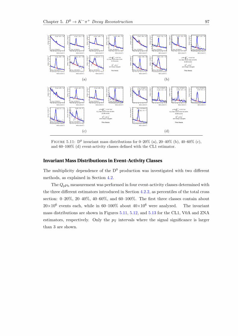
Chapter 5. D0 → K−π+ Decay Reconstruction 97
= 5.02 TeVNN
spPb,
CL1 Mult. Event Class 020%
20.7M events
and charge conjugate
+π
K→
0D
This thesis
)2
c) (GeV/π(KM
1.75 1.8 1.85 1.9 1.95 2 2.05
2 cE
ntrie
s / 6
MeV
/
0
200
400
600
800
1000
1200
1400
1600
c<2 GeV/T
p1<
83±) = 597 σS (3
)2
c) (GeV/π(KM
1.75 1.8 1.85 1.9 1.95 2 2.05
2 cE
ntrie
s / 6
MeV
/
0
100
200
300
400
500
600
700
800
900
c<4 GeV/T
p2<
75±) = 1751 σS (3
)2
c) (GeV/π(KM
1.75 1.8 1.85 1.9 1.95 2
2 cE
ntrie
s / 1
2 M
eV/
0
200
400
600
800
1000
1200
1400
c<6 GeV/T
p4<
76±) = 1502 σS (3
)2
c) (GeV/π(KM
1.7 1.8 1.9 2 2.1
2 cE
ntrie
s / 1
2 M
eV/
0
50
100
150
200
250
c<8 GeV/T
p6<
30±) = 446 σS (3
)2
c) (GeV/π(KM
1.7 1.75 1.8 1.85 1.9 1.95 2 2.05 2.1
2 cE
ntrie
s / 2
4 M
eV/
0
50
100
150
200
250
300
c<12 GeV/T
p8<
25±) = 356 σS (3
)2
c) (GeV/π(KM
1.7 1.75 1.8 1.85 1.9 1.95 2 2.05 2.1
2 cE
ntrie
s / 2
4 M
eV/
0
20
40
60
80
100
c<16 GeV/T
p12<
26±) = 141 σS (3
)2
c) (GeV/π(KM
1.7 1.8 1.9 2 2.1
2 cE
ntrie
s / 3
0 M
eV/
0
10
20
30
40
50
c<24 GeV/T
p16<
17±) = 67 σS (3
(a)
= 5.02 TeVNN
spPb,
CL1 Mult. Event Class 2040%
20.6M events
and charge conjugate
+π
K→
0D
This thesis
)2
c) (GeV/π(KM
1.75 1.8 1.85 1.9 1.95 2 2.05
2 cE
ntrie
s / 6
MeV
/
0
50
100
150
200
250
300
350
400
450
c<2 GeV/T
p1<
52±) = 308 σS (3
)2
c) (GeV/π(KM
1.75 1.8 1.85 1.9 1.95 2 2.05
2 cE
ntrie
s / 6
MeV
/
0
50
100
150
200
250
300
350
c<4 GeV/T
p2<
41±) = 751 σS (3
)2
c) (GeV/π(KM
1.7 1.8 1.9 2 2.1
2 cE
ntrie
s / 1
2 M
eV/
0
50
100
150
200
250
300
350
400
450
500
c<6 GeV/T
p4<
44±) = 726 σS (3
)2
c) (GeV/π(KM
1.7 1.75 1.8 1.85 1.9 1.95 2 2.05 2.1
2 cE
ntrie
s / 1
5 M
eV/
0
20
40
60
80
100
120
140
c<8 GeV/T
p6<
19±) = 237 σS (3
)2
c) (GeV/π(KM
1.6 1.7 1.8 1.9 2 2.1
2 cE
ntrie
s / 2
4 M
eV/
0
20
40
60
80
100
120
140
c<12 GeV/T
p8<
19±) = 198 σS (3
)2
c) (GeV/π(KM
1.7 1.75 1.8 1.85 1.9 1.95 2 2.05 2.1
2 cE
ntrie
s / 2
4 M
eV/
0
10
20
30
40
50
c<16 GeV/T
p12<
14±) = 101 σS (3
(b)
= 5.02 TeVNN
spPb,
CL1 Mult. Event Class 4060%20.8M events
and charge conjugate
+π
K→
0D
This thesis
)2
c) (GeV/π(KM
1.75 1.8 1.85 1.9 1.95 2 2.05
2 cE
ntrie
s / 6
MeV
/
0
50
100
150
200
250
c<2 GeV/T
p1<
31±) = 155 σS (3
)2
c) (GeV/π(KM
1.75 1.8 1.85 1.9 1.95 2
2 cE
ntrie
s / 1
2 M
eV/
0
50
100
150
200
250
300
350
c<4 GeV/T
p2<
31±) = 446 σS (3
)2
c) (GeV/π(KM
1.75 1.8 1.85 1.9 1.95 2
2 cE
ntrie
s / 1
2 M
eV/
0
50
100
150
200
250
c<6 GeV/T
p4<
29±) = 389 σS (3
)2
c) (GeV/π(KM
1.7 1.75 1.8 1.85 1.9 1.95 2 2.05 2.1
2 cE
ntrie
s / 1
5 M
eV/
0
10
20
30
40
50
60
70
c<8 GeV/T
p6<
14±) = 133 σS (3
)2
c) (GeV/π(KM
1.7 1.75 1.8 1.85 1.9 1.95 2 2.05 2.1
2 cE
ntrie
s / 1
5 M
eV/
0
10
20
30
40
50
c<12 GeV/T
p8<
12±) = 97 σS (3
)2
c) (GeV/π(KM
1.6 1.7 1.8 1.9 2 2.1
2 cE
ntrie
s / 3
0 M
eV/
0
5
10
15
20
25
30
c<16 GeV/T
p12<
8±) = 28 σS (3
(c)
= 5.02 TeVNN
spPb,
CL1 Mult. Event Class 60100%
38.8M events
and charge conjugate
+π
K→
0D
This thesis
)2
c) (GeV/π(KM
1.75 1.8 1.85 1.9 1.95 2
2 cE
ntrie
s / 1
2 M
eV/
0
20
40
60
80
100
120
140
160
180
c<2 GeV/T
p1< 22±) = 118 σS (3
)2
c) (GeV/π(KM
1.75 1.8 1.85 1.9 1.95 2 2.05
2 cE
ntrie
s / 6
MeV
/
0
10
20
30
40
50
60
70
80
90
100
c<4 GeV/T
p2< 18±) = 213 σS (3
)2
c) (GeV/π(KM
1.75 1.8 1.85 1.9 1.95 2 2.05
2 cE
ntrie
s / 6
MeV
/
0
10
20
30
40
50
60
70
c<6 GeV/T
p4< 15±) = 164 σS (3
)2
c) (GeV/π(KM
1.7 1.75 1.8 1.85 1.9 1.95 2 2.05 2.1
2 cE
ntrie
s / 2
4 M
eV/
0
10
20
30
40
50
60
70
c<8 GeV/T
p6< 9±) = 80 σS (3
)2
c) (GeV/π(KM
1.7 1.75 1.8 1.85 1.9 1.95 2 2.05 2.1 2.15
2 cE
ntrie
s / 3
6 M
eV/
0
5
10
15
20
25
30
35
40
c<12 GeV/T
p8<
7±) = 37 σS (3
(d)
Figure 5.11: D0 invariant mass distributions for 0–20% (a), 20–40% (b), 40–60% (c),and 60–100% (d) event-activity classes defined with the CL1 estimator.
Invariant Mass Distributions in Event-Activity Classes
The multiplicity dependence of the D0 production was investigated with two different
methods, as explained in Section 4.2.
The QpPb measurement was performed in four event-activity classes determined with
the three different estimators introduced in Section 4.2.2, as percentiles of the total cross
section: 0–20%, 20–40%, 40–60%, and 60–100%. The first three classes contain about
20×106 events each, while in 60–100% about 40×106 were analyzed. The invariant
mass distributions are shown in Figures 5.11, 5.12, and 5.13 for the CL1, V0A and ZNA
estimators, respectively. Only the pT intervals where the signal significance is larger
than 3 are shown.

Chapter 5. D0 → K−π+ Decay Reconstruction 98
= 5.02 TeVNN
spPb,
V0A Mult. Event Class 020%20.6M events
and charge conjugate
+π
K→
0D
This thesis
)2
c) (GeV/π(KM
1.8 1.85 1.9 1.95 2
2 cE
ntrie
s / 6
MeV
/
0
200
400
600
800
1000
1200
c<2 GeV/T
p1<
85±) = 579 σS (3
)2
c) (GeV/π(KM
1.75 1.8 1.85 1.9 1.95 2 2.05
2 cE
ntrie
s / 6
MeV
/
0
100
200
300
400
500
600
700
c<4 GeV/T
p2<
69±) = 1499 σS (3
)2
c) (GeV/π(KM
1.75 1.8 1.85 1.9 1.95 2
2 cE
ntrie
s / 1
2 M
eV/
0
200
400
600
800
1000
1200
c<6 GeV/T
p4<
70±) = 1284 σS (3
)2
c) (GeV/π(KM
1.7 1.8 1.9 2 2.1
2 cE
ntrie
s / 1
2 M
eV/
0
20
40
60
80
100
120
140
160
180
200
220
c<8 GeV/T
p6<
28±) = 358 σS (3
)2
c) (GeV/π(KM
1.7 1.75 1.8 1.85 1.9 1.95 2 2.05 2.1
2 cE
ntrie
s / 2
4 M
eV/
0
20
40
60
80
100
120
140
160
180
200
220
240
c<12 GeV/T
p8<
23±) = 319 σS (3
)2
c) (GeV/π(KM
1.7 1.75 1.8 1.85 1.9 1.95 2 2.05 2.1
2 cE
ntrie
s / 2
4 M
eV/
0
10
20
30
40
50
60
70
80
c<16 GeV/T
p12<
20±) = 120 σS (3
)2
c) (GeV/π(KM
1.7 1.8 1.9 2 2.1
2 cE
ntrie
s / 3
0 M
eV/
0
5
10
15
20
25
30
35
40
45
c<24 GeV/T
p16<
14±) = 57 σS (3
(a)
= 5.02 TeVNN
spPb,
V0A Mult. Event Class 2040%
20.7M events
and charge conjugate
+π
K→
0D
This thesis
)2
c) (GeV/π(KM
1.75 1.8 1.85 1.9 1.95 2
2 cE
ntrie
s / 1
2 M
eV/
0
200
400
600
800
1000
c<2 GeV/T
p1<
75±) = 294 σS (3
)2
c) (GeV/π(KM
1.75 1.8 1.85 1.9 1.95 2 2.05
2 cE
ntrie
s / 6
MeV
/
0
50
100
150
200
250
300
350
400
c<4 GeV/T
p2<
44±) = 825 σS (3
)2
c) (GeV/π(KM
1.75 1.8 1.85 1.9 1.95 2
2 cE
ntrie
s / 1
2 M
eV/
0
100
200
300
400
500
600
c<6 GeV/T
p4<
47±) = 781 σS (3
)2
c) (GeV/π(KM
1.7 1.75 1.8 1.85 1.9 1.95 2 2.05 2.1
2 cE
ntrie
s / 1
5 M
eV/
0
20
40
60
80
100
120
140
160
c<8 GeV/T
p6<
21±) = 258 σS (3
)2
c) (GeV/π(KM
1.7 1.75 1.8 1.85 1.9 1.95 2 2.05 2.1
2 cE
ntrie
s / 2
4 M
eV/
0
20
40
60
80
100
120
140
c<12 GeV/T
p8<
16±) = 158 σS (3
)2
c) (GeV/π(KM
1.6 1.7 1.8 1.9 2 2.1
2 cE
ntrie
s / 2
4 M
eV/
0
10
20
30
40
50
60
c<16 GeV/T
p12<
16±) = 89 σS (3
(b)
= 5.02 TeVNN
spPb,
V0A Mult. Event Class 4060%
20.7M events
and charge conjugate
+π
K→
0D
This thesis
)2
c) (GeV/π(KM
1.75 1.8 1.85 1.9 1.95 2 2.05
2 cE
ntrie
s / 9
MeV
/
0
50
100
150
200
250
300
350
c<2 GeV/T
p1<
32±) = 150 σS (3
)2
c) (GeV/π(KM
1.75 1.8 1.85 1.9 1.95 2 2.05
2 cE
ntrie
s / 6
MeV
/
0
20
40
60
80
100
120
140
160
180
200
220
c<4 GeV/T
p2<
35±) = 522 σS (3
)2
c) (GeV/π(KM
1.75 1.8 1.85 1.9 1.95 2 2.05
2 cE
ntrie
s / 6
MeV
/
0
20
40
60
80
100
120
140
160
180
c<6 GeV/T
p4<
35±) = 502 σS (3
)2
c) (GeV/π(KM
1.7 1.8 1.9 2 2.1
2 cE
ntrie
s / 1
2 M
eV/
0
10
20
30
40
50
60
70
80
90
c<8 GeV/T
p6<
17±) = 177 σS (3
)2
c) (GeV/π(KM
1.7 1.75 1.8 1.85 1.9 1.95 2 2.05 2.1 2.15
2 cE
ntrie
s / 1
2 M
eV/
0
10
20
30
40
50
c<12 GeV/T
p8<
14±) = 125 σS (3
)2
c) (GeV/π(KM
1.7 1.75 1.8 1.85 1.9 1.95 2 2.05 2.1
2 cE
ntrie
s / 2
4 M
eV/
0
5
10
15
20
25
30
c<16 GeV/T
p12<
12±) = 28 σS (3
(c)
= 5.02 TeVNN
spPb,
V0A Mult. Event Class 60100%
38.8M events
and charge conjugate
+π
K→
0D
This thesis
)2
) (GeV/cπInvariant Mass (K
1.75 1.8 1.85 1.9 1.95 2
2E
ntrie
s / 1
2 M
eV/c
0
50
100
150
200
250
c<2 GeV/T
p1<
35±) = 152 σS (3
)2
) (GeV/cπInvariant Mass (K
1.75 1.8 1.85 1.9 1.95 2
2E
ntrie
s / 1
2 M
eV/c
0
50
100
150
200
250
c<4 GeV/T
p2<
24±) = 326 σS (3
)2
) (GeV/cπInvariant Mass (K
1.75 1.8 1.85 1.9 1.95 2
2E
ntrie
s / 1
5 M
eV/c
0
50
100
150
200
250
c<6 GeV/T
p4<
25±) = 273 σS (3
)2
) (GeV/cπInvariant Mass (K
1.7 1.75 1.8 1.85 1.9 1.95 2 2.05 2.1
2E
ntrie
s / 2
4 M
eV/c
0
10
20
30
40
50
60
70
80
90
c<8 GeV/T
p6<
13±) = 111 σS (3
)2
) (GeV/cπInvariant Mass (K
1.7 1.75 1.8 1.85 1.9 1.95 2 2.05 2.1
2E
ntrie
s / 1
5 M
eV/c
0
5
10
15
20
25
30
35
40
45
c<12 GeV/T
p8<
11±) = 95 σS (3
)2
) (GeV/cπInvariant Mass (K
1.7 1.75 1.8 1.85 1.9 1.95 2 2.05 2.1 2.15
2E
ntrie
s / 3
0 M
eV/c
0
5
10
15
20
25
30
c<16 GeV/T
p12<
8±) = 27 σS (3
(d)
Figure 5.12: D0 invariant mass distributions for 0–20% (a), 20–40% (b), 40–60% (c),and 60–100% (d) event-activity classes defined with the V0A estimator.
= 5.02 TeVNN
spPb,
ZN Energy Event Class 020%
20.6M events
and charge conjugate
+π
K→
0D
This thesis
)2
c) (GeV/π(KM
1.75 1.8 1.85 1.9 1.95 2 2.05
2 cE
ntrie
s / 6
MeV
/
0
200
400
600
800
1000
c<2 GeV/T
p1<
65±) = 444 σS (3
)2
c) (GeV/π(KM
1.75 1.8 1.85 1.9 1.95 2 2.05
2 cE
ntrie
s / 6
MeV
/
0
100
200
300
400
500
600
c<4 GeV/T
p2<
58±) = 1077 σS (3
)2
c) (GeV/π(KM
1.75 1.8 1.85 1.9 1.95 2
2 cE
ntrie
s / 1
2 M
eV/
0
100
200
300
400
500
600
700
c<6 GeV/T
p4<
56±) = 1003 σS (3
)2
c) (GeV/π(KM
1.75 1.8 1.85 1.9 1.95 2
2 cE
ntrie
s / 1
2 M
eV/
0
20
40
60
80
100
120
140
160
180
c<8 GeV/T
p6<
26±) = 317 σS (3
)2
c) (GeV/π(KM
1.7 1.75 1.8 1.85 1.9 1.95 2 2.05 2.1
2 cE
ntrie
s / 1
5 M
eV/
0
20
40
60
80
100
120
140
c<12 GeV/T
p8<
20±) = 247 σS (3
)2
c) (GeV/π(KM
1.75 1.8 1.85 1.9 1.95 2 2.05
2 cE
ntrie
s / 2
4 M
eV/
0
10
20
30
40
50
60
70
80
c<16 GeV/T
p12<
17±) = 104 σS (3
)2
c) (GeV/π(KM
1.75 1.8 1.85 1.9 1.95 2 2.05
2 cE
ntrie
s / 2
4 M
eV/
0
5
10
15
20
25
c<24 GeV/T
p16<
13±) = 35 σS (3
(a)
= 5.02 TeVNN
spPb,
ZN Energy Event Class 2040%20.6M events
and charge conjugate
+π
K→
0D
This thesis
)2
c) (GeV/π(KM
1.75 1.8 1.85 1.9 1.95 2
2 cE
ntrie
s / 5
MeV
/
0
100
200
300
400
500
600
c<2 GeV/T
p1<
65±) = 377 σS (3
)2
c) (GeV/π(KM
1.75 1.8 1.85 1.9 1.95 2 2.05
2 cE
ntrie
s / 8
MeV
/
0
100
200
300
400
500
c<4 GeV/T
p2<
51±) = 955 σS (3
)2
c) (GeV/π(KM
1.75 1.8 1.85 1.9 1.95 2 2.05
2 cE
ntrie
s / 8
MeV
/
0
50
100
150
200
250
300
350
c<6 GeV/T
p4<
43±) = 706 σS (3
)2
c) (GeV/π(KM
1.75 1.8 1.85 1.9 1.95 2 2.05
2 cE
ntrie
s / 8
MeV
/
0
10
20
30
40
50
60
70
80
90
c<8 GeV/T
p6<
21±) = 243 σS (3
)2
c) (GeV/π(KM
1.7 1.75 1.8 1.85 1.9 1.95 2 2.05 2.1
2 cE
ntrie
s / 1
2 M
eV/
0
10
20
30
40
50
60
70
c<12 GeV/T
p8<
17±) = 189 σS (3
)2
c) (GeV/π(KM
1.7 1.75 1.8 1.85 1.9 1.95 2 2.05
2 cE
ntrie
s / 2
4 M
eV/
0
10
20
30
40
50
60
c<16 GeV/T
p12<
20±) = 103 σS (3
)2
c) (GeV/π(KM
1.7 1.75 1.8 1.85 1.9 1.95 2 2.05
2 cE
ntrie
s / 2
5 M
eV/
0
2
4
6
8
10
12
14
16
18
20
22
c<24 GeV/T
p16<
11±) = 31 σS (3
(b)
= 5.02 TeVNN
spPb,
ZN Energy Event Class 4060%20.4M events
and charge conjugate
+π
K→
0D
This thesis
)2
c) (GeV/π(KM
1.75 1.8 1.85 1.9 1.95 2 2.05
2 cE
ntrie
s / 6
MeV
/
0
100
200
300
400
500
600
700
800
c<2 GeV/T
p1<
58±) = 260 σS (3
)2
c) (GeV/π(KM
1.75 1.8 1.85 1.9 1.95 2 2.05
2 cE
ntrie
s / 6
MeV
/
0
50
100
150
200
250
300
c<4 GeV/T
p2<
40±) = 606 σS (3
)2
c) (GeV/π(KM
1.75 1.8 1.85 1.9 1.95 2
2 cE
ntrie
s / 1
2 M
eV/
0
50
100
150
200
250
300
350
400
c<6 GeV/T
p4<
35±) = 483 σS (3
)2
c) (GeV/π(KM
1.75 1.8 1.85 1.9 1.95 2
2 cE
ntrie
s / 1
2 M
eV/
0
20
40
60
80
100
120
c<8 GeV/T
p6<
17±) = 185 σS (3
)2
c) (GeV/π(KM
1.7 1.75 1.8 1.85 1.9 1.95 2 2.05 2.1
2 cE
ntrie
s / 1
5 M
eV/
0
10
20
30
40
50
60
70
c<12 GeV/T
p8<
16±) = 133 σS (3
)2
c) (GeV/π(KM
1.7 1.75 1.8 1.85 1.9 1.95 2 2.05
2 cE
ntrie
s / 2
4 M
eV/
0
5
10
15
20
25
c<16 GeV/T
p12<
11±) = 34 σS (3
)2
c) (GeV/π(KM
1.7 1.75 1.8 1.85 1.9 1.95 2 2.05
2 cE
ntrie
s / 2
8 M
eV/
0
2
4
6
8
10
12
14
16
18
20
22
c<24 GeV/T
p16<
10±) = 35 σS (3
(c)
= 5.02 TeVNN
spPb,
ZN Energy Event Class 60100%
38.9M events
and charge conjugate
+π
K→
0D
This thesis
)2
c) (GeV/π(KM
1.75 1.8 1.85 1.9 1.95 2 2.05
2 cE
ntrie
s / 6
MeV
/
0
50
100
150
200
250
300
c<2 GeV/T
p1<
40±) = 249 σS (3
)2
c) (GeV/π(KM
1.75 1.8 1.85 1.9 1.95 2 2.05
2 cE
ntrie
s / 6
MeV
/
0
20
40
60
80
100
120
140
160
180
200
220
c<4 GeV/T
p2<
34±) = 522 σS (3
)2
c) (GeV/π(KM
1.75 1.8 1.85 1.9 1.95 2
2 cE
ntrie
s / 1
2 M
eV/
0
50
100
150
200
250
300
c<6 GeV/T
p4<
30±) = 419 σS (3
)2
c) (GeV/π(KM
1.75 1.8 1.85 1.9 1.95 2
2 cE
ntrie
s / 1
2 M
eV/
0
10
20
30
40
50
60
70
80
c<8 GeV/T
p6<
16±) = 180 σS (3
)2
c) (GeV/π(KM
1.7 1.75 1.8 1.85 1.9 1.95 2 2.05 2.1
2 cE
ntrie
s / 1
5 M
eV/
0
10
20
30
40
50
60
c<12 GeV/T
p8<
14±) = 120 σS (3
)2
c) (GeV/π(KM
1.75 1.8 1.85 1.9 1.95 2 2.05 2.1
2 cE
ntrie
s / 3
0 M
eV/
0
5
10
15
20
25
30
35
40
45
c<16 GeV/T
p12<
11±) = 36 σS (3
(d)
Figure 5.13: D0 invariant mass distributions for 0–20% (a), 20–40% (b), 40–60% (c),and 60–100% (d) event-activity classes defined with the ZNA estimator.

Chapter 5. D0 → K−π+ Decay Reconstruction 99
(cm)vtxz
10 8 6 4 2 0 2 4 6 8 10
unco
rrec
ted
trac
klet
sN
0
10
20
30
40
50
60
70
0
2000
4000
6000
8000
10000
12000
(cm)vtxz
10 8 6 4 2 0 2 4 6 8 10
corr
ecte
dtr
ackl
ets
N
0
10
20
30
40
50
60
70
0
2000
4000
6000
8000
10000
12000
ALICE Preliminary
= 5.02 TeVNNspPb,
| < 1.0η|
ALI−PREL−76693
Figure 5.14: zvtx distributions of multiplicity estimated with Ntracklets in |η| < 1. Inthe left panel is reported the raw distribution which demonstrates the variation of theSPD acceptance with time and zvtx. In the right panel the corrected distribution isshown.
Invariant Mass Distributions in Multiplicity Intervals
The second observable used to investigate the multiplicity dependence of the D0 pro-
duction (Section 4.2.3) requires the extraction of the raw yields in charged-particle mul-
tiplicity intervals. The number of tracklets in |η| < 1.0 measured with the SPD detector
was used to define the multiplicity intervals. The pseudorapidity acceptance of the SPD
depends on the position of the interaction vertex along the beam line, zvtx. In addition,
it varied during the data taking due to the variation of the number of inactive channels.
The detector response was equalized by means of a data-driven correction, which was
applied on an event-by-event basis depending on zvtx and time. The variation of the SPD
acceptance as a function of zvtx can be verified with the two-dimensional distribution of
the number of tracklets (Ntracklets) as a function of the position of the primary vertex
along the z direction, shown in Figure 5.14. The profile of the distribution, defined
as the mean Ntracklets as a function of zvtx, is shown as a black line. The raw profile,
shown in the left panel, was applied event-by-event, in order to correct the multiplicity
distribution. The formula used for the correction was:
N correctedtracklets (zvtx) =
〈N reftracklets〉
〈Nuncorrectedtracklets (zvtx)〉 ·N
uncorrectedtracklets (zvtx) , (5.2)
where 〈N reftracklets〉 is the mean number of tracklets in a given zvtx interval chosen as refer-
ence. Nuncorrectedtracklets (zvtx) is the number of tracklets for events with vertex at a given value

Chapter 5. D0 → K−π+ Decay Reconstruction 100
primarychN
0 50 100 150 200 250
SP
Dtr
ackl
ets
N
0
50
100
150
200
1
10
210
310
410
510
1
10
210
310
410
510
ALICE Preliminary = 5.02 TeVNNspPb,
| < 1.0η|
ALI−PREL−76792
Figure 5.15: SPD Ntracklets multiplicity as a function of the primary charged-particlemultiplicity in Monte Carlo simulations. The black line indicates the profile of thedistribution: linear proportionality was found with a factor of 0.75.
of z for the data taking period under consideration, and 〈Nuncorrectedtracklets (zvtx)〉 its mean
value. In the correction procedure, the Poisson statistics is employed to get an inte-
ger value for N correctedtracklets (zvtx) starting from the value of (〈N ref
tracklets〉/〈Nuncorrectedtracklets (zvtx)〉) ·
Nuncorrectedtracklets (zvtx). The resulting N corrected
tracklets distribution, reported in the right panel of
Figure 5.14, is uniform in zvtx, with an average N reftracklets value being set at the prede-
termined reference multiplicity.
The multiplicity intervals were defined on the basis of the corrected Ntracklets distri-
butions and then converted to intervals of relative charged-particle multiplicity, (dNch/dη)/
〈dNch/dη〉. The conversion was done exploiting the proportionality of the number of
reconstructed tracklets to the generated charged primary particles Nprimarych observed in
the simulations for |η| < 1.0. It was found that there is a linear relation between Ntracklets
and Nprimarych , with a factor of proportionality (Ntracklets/N
primarych ) = 0.75 (Figure 5.15).
The Ntracklets values were divided by the proportionality factor to convert to Nprimarych ,
and then by a further factor of two (the width of the pseudorapidity range studied) to
give dNch/dη. The average pseudorapidity density of charged particles in the considered
range, 〈dNch/dη〉, used to obtain the relative multiplicity in each Ntracklets interval, is
17.64 ± 0.01 (stat.) ± 0.15 (syst.), as measured in inelastic p–Pb collisions producing
at least one charged particle in |η| < 1 [109, 110]. The considered Ntracklets intervals
and the corresponding relative charged-particle multiplicity ranges are summarized in
Table 5.5.
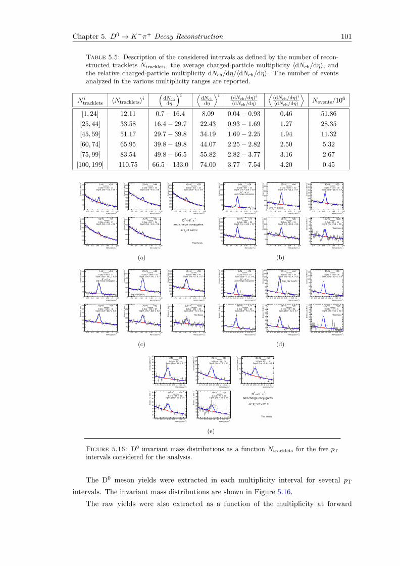
Chapter 5. D0 → K−π+ Decay Reconstruction 101
Table 5.5: Description of the considered intervals as defined by the number of recon-structed tracklets Ntracklets, the average charged-particle multiplicity 〈dNch/dη〉, andthe relative charged-particle multiplicity dNch/dη/〈dNch/dη〉. The number of eventsanalyzed in the various multiplicity ranges are reported.
N itracklets 〈Ntracklets〉i
(dNch
dη
)i ⟨dNch
dη
⟩i(dNch/dη)i
〈dNch/dη〉
⟨(dNch/dη)i
〈dNch/dη〉
⟩Nevents/106
[1, 24] 12.11 0.7− 16.4 8.09 0.04− 0.93 0.46 51.86
[25, 44] 33.58 16.4− 29.7 22.43 0.93− 1.69 1.27 28.35
[45, 59] 51.17 29.7− 39.8 34.19 1.69− 2.25 1.94 11.32
[60, 74] 65.95 39.8− 49.8 44.07 2.25− 2.82 2.50 5.32
[75, 99] 83.54 49.8− 66.5 55.82 2.82− 3.77 3.16 2.67
[100, 199] 110.75 66.5− 133.0 74.00 3.77− 7.54 4.20 0.45
)2
c) (GeV/π(KM1.75 1.8 1.85 1.9 1.95 2 2.05
2 cE
ntrie
s / 6
MeV
/
0
50
100
150
200
250 <24tracklets
N1<
24±) = 166 σS (3 0.8±) = 6.0 σSignif. (3
)2
c) (GeV/π(KM1.75 1.8 1.85 1.9 1.95 2 2.05
2 cE
ntrie
s / 6
MeV
/
0
100
200
300
400
500
600
700
800 <44tracklets
N25<
45±) = 348 σS (3 0.8±) = 6.6 σSignif. (3
)2
c) (GeV/π(KM1.75 1.8 1.85 1.9 1.95 2 2.05
2 cE
ntrie
s / 6
MeV
/
0
100
200
300
400
500
600
700
800 <59tracklets
N45<
43±) = 312 σS (3 0.8±) = 6.1 σSignif. (3
)2
c) (GeV/π(KM1.75 1.8 1.85 1.9 1.95 2 2.05
2 cE
ntrie
s / 6
MeV
/
0
100
200
300
400
500
600 <74tracklets
N60< 37±) = 148 σS (3
0.8±) = 3.3 σSignif. (3
)2
c) (GeV/π(KM1.75 1.8 1.85 1.9 1.95 2 2.05
2 cE
ntrie
s / 6
MeV
/
0
100
200
300
400
500 <99tracklets
N75< 34±) = 157 σS (3
0.8±) = 3.8 σSignif. (3
+π
K→
0D
and charge conjugates
This thesis
c<2 GeV/T
p1<
(a)
)2
c) (GeV/π(KM1.75 1.8 1.85 1.9 1.95 2 2.05
2 cE
ntrie
s / 6
MeV
/
0
50
100
150
200
250 <24tracklets
N1<
24±) = 427 σS (3 0.6±) = 15.9 σSignif. (3
+π
K→
0D
and charge conjugates
)2
c) (GeV/π(KM1.75 1.8 1.85 1.9 1.95 2 2.05
2 cE
ntrie
s / 6
MeV
/
0
100
200
300
400
500<44
trackletsN25<
42±) = 1001 σS (3 0.7±) = 21.2 σSignif. (3
c<4 GeV/T
p2<
)2
c) (GeV/π(KM1.75 1.8 1.85 1.9 1.95 2 2.05
2 cE
ntrie
s / 6
MeV
/
0
50
100
150
200
250
300
350
400
450 <59tracklets
N45<
40±) = 726 σS (3 0.7±) = 16.3 σSignif. (3
)2
c) (GeV/π(KM1.75 1.8 1.85 1.9 1.95 2 2.05
2 cE
ntrie
s / 6
MeV
/
0
50
100
150
200
250
300
350 <74tracklets
N60< 36±) = 581 σS (3
0.7±) = 14.5 σSignif. (3
)2
c) (GeV/π(KM1.75 1.8 1.85 1.9 1.95 2 2.05
2 cE
ntrie
s / 6
MeV
/
0
50
100
150
200
250 <99tracklets
N75< 31±) = 357 σS (3
0.8±) = 10.3 σSignif. (3
)2
c) (GeV/π(KM1.75 1.8 1.85 1.9 1.95 2 2.05
2 cE
ntrie
s / 6
MeV
/
0
10
20
30
40
50
60
70
80 <199tracklets
N100< 16±) = 95 σS (3
0.8±) = 5.1 σSignif. (3
This thesis
(b)
)2
c) (GeV/π(KM1.75 1.8 1.85 1.9 1.95 2 2.05
2 cE
ntrie
s / 6
MeV
/
0
50
100
150
200
250 <24tracklets
N1<
27±) = 562 σS (3 0.6±) = 18.1 σSignif. (3
+π
K→
0D
and charge conjugates
)2
c) (GeV/π(KM1.75 1.8 1.85 1.9 1.95 2 2.05
2 cE
ntrie
s / 6
MeV
/
0
100
200
300
400
500<44
trackletsN25<
51±) = 1368 σS (3 0.7±) = 24.1 σSignif. (3
c<8 GeV/T
p4<
)2
c) (GeV/π(KM1.75 1.8 1.85 1.9 1.95 2 2.05
2 cE
ntrie
s / 6
MeV
/
0
50
100
150
200
250
300
350
400
450 <59tracklets
N45<
47±) = 940 σS (3 0.7±) = 17.8 σSignif. (3
)2
c) (GeV/π(KM1.75 1.8 1.85 1.9 1.95 2 2.05
2 cE
ntrie
s / 6
MeV
/
0
50
100
150
200
250
300
350 <74tracklets
N60< 42±) = 639 σS (3
0.8±) = 13.7 σSignif. (3
)2
c) (GeV/π(KM1.75 1.8 1.85 1.9 1.95 2 2.05
2 cE
ntrie
s / 6
MeV
/
0
50
100
150
200
250
300 <99tracklets
N75< 37±) = 452 σS (3
0.8±) = 10.8 σSignif. (3
)2
c) (GeV/π(KM1.75 1.8 1.85 1.9 1.95 2 2.05
2 cE
ntrie
s / 6
MeV
/
0
20
40
60
80
100 <199tracklets
N100< 20±) = 105 σS (3
0.8±) = 4.6 σSignif. (3
This thesis
(c)
)2
c) (GeV/π(KM1.7 1.75 1.8 1.85 1.9 1.95 2 2.05 2.1
2 cE
ntrie
s / 1
5 M
eV/
0
10
20
30
40
50
60
70
80 <24tracklets
N1<
10±) = 82 σS (3 0.6±) = 7.1 σSignif. (3
+π
K→
0D
and charge conjugates
)2
c) (GeV/π(KM1.7 1.75 1.8 1.85 1.9 1.95 2 2.05 2.1
2 cE
ntrie
s / 1
5 M
eV/
0
20
40
60
80
100
120
140
160 <44tracklets
N25<
18±) = 252 σS (3 0.6±) = 12.4 σSignif. (3
c<12 GeV/T
p8<
)2
c) (GeV/π(KM1.7 1.75 1.8 1.85 1.9 1.95 2 2.05 2.1
2 cE
ntrie
s / 1
5 M
eV/
0
20
40
60
80
100
120
140 <59tracklets
N45<
16±) = 184 σS (3 0.6±) = 10.4 σSignif. (3
)2
c) (GeV/π(KM1.7 1.75 1.8 1.85 1.9 1.95 2 2.05 2.1
2 cE
ntrie
s / 1
5 M
eV/
0
20
40
60
80
100 <74tracklets
N60< 13±) = 110 σS (3
0.7±) = 7.5 σSignif. (3
)2
c) (GeV/π(KM1.7 1.75 1.8 1.85 1.9 1.95 2 2.05 2.1
2 cE
ntrie
s / 1
5 M
eV/
0
10
20
30
40
50
60
70 <99tracklets
N75< 11±) = 78 σS (3
0.7±) = 6.3 σSignif. (3
)2
c) (GeV/π(KM1.7 1.75 1.8 1.85 1.9 1.95 2 2.05 2.1
2 cE
ntrie
s / 1
5 M
eV/
0
2
4
6
8
10
12
14
16
18
20
22 <199tracklets
N100< 6±) = 27 σS (3
0.6±) = 3.9 σSignif. (3
This thesis
(d)
)2
c) (GeV/π(KM1.7 1.75 1.8 1.85 1.9 1.95 2 2.05 2.1
2 cE
ntrie
s / 2
4 M
eV/
0
5
10
15
20
25
30
35
40
45<24
trackletsN1<
9±) = 50 σS (3 0.7±) = 4.8 σSignif. (3
)2
c) (GeV/π(KM1.7 1.75 1.8 1.85 1.9 1.95 2 2.05 2.1
2 cE
ntrie
s / 2
4 M
eV/
0
20
40
60
80
100
120
140 <44tracklets
N25<
18±) = 150 σS (3 0.7±) = 7.6 σSignif. (3
)2
c) (GeV/π(KM1.7 1.75 1.8 1.85 1.9 1.95 2 2.05 2.1
2 cE
ntrie
s / 2
4 M
eV/
0
20
40
60
80
100 <59tracklets
N45<
16±) = 95 σS (3 0.8±) = 5.4 σSignif. (3
)2
c) (GeV/π(KM1.7 1.75 1.8 1.85 1.9 1.95 2 2.05 2.1
2 cE
ntrie
s / 2
4 M
eV/
0
10
20
30
40
50
60
70
80 <74tracklets
N60< 13±) = 58 σS (3
0.8±) = 3.9 σSignif. (3
)2
c) (GeV/π(KM1.7 1.75 1.8 1.85 1.9 1.95 2 2.05 2.1
2 cE
ntrie
s / 1
5 M
eV/
0
5
10
15
20
25
30
35
40
45<99
trackletsN75<
12±) = 47 σS (3 0.8±) = 3.6 σSignif. (3
+π
K→
0D
and charge conjugates
This thesis
c<24 GeV/T
p12<
(e)
Figure 5.16: D0 invariant mass distributions as a function Ntracklets for the five pT
intervals considered for the analysis.
The D0 meson yields were extracted in each multiplicity interval for several pT
intervals. The invariant mass distributions are shown in Figure 5.16.
The raw yields were also extracted as a function of the multiplicity at forward
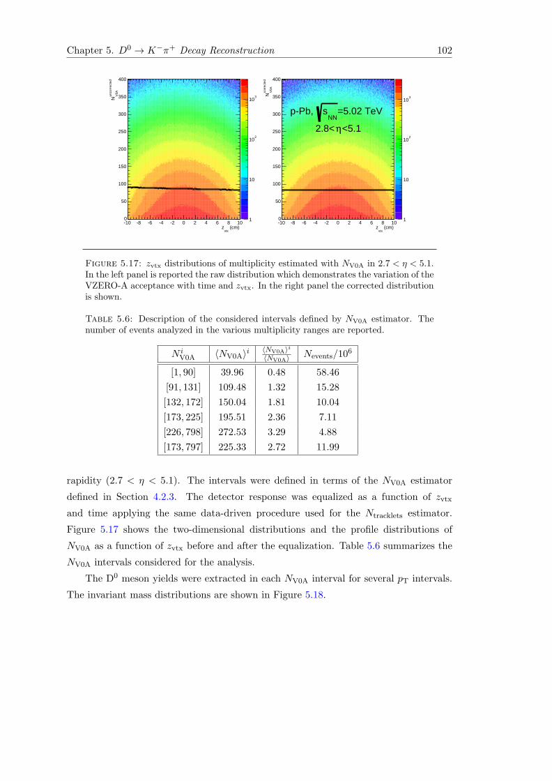
Chapter 5. D0 → K−π+ Decay Reconstruction 102
(cm)vtx
z10 8 6 4 2 0 2 4 6 8 10
unco
rrec
ted
V0A
N
0
50
100
150
200
250
300
350
400
1
10
210
310
(cm)vtx
z10 8 6 4 2 0 2 4 6 8 10
corr
ecte
d
V0A
N
0
50
100
150
200
250
300
350
400
1
10
210
310
=5.02 TeVNN
spPb,
<5.1η2.8<
Figure 5.17: zvtx distributions of multiplicity estimated with NV0A in 2.7 < η < 5.1.In the left panel is reported the raw distribution which demonstrates the variation of theVZERO-A acceptance with time and zvtx. In the right panel the corrected distributionis shown.
Table 5.6: Description of the considered intervals defined by NV0A estimator. Thenumber of events analyzed in the various multiplicity ranges are reported.
N iV0A 〈NV0A〉i 〈NV0A〉i
〈NV0A〉 Nevents/106
[1, 90] 39.96 0.48 58.46
[91, 131] 109.48 1.32 15.28
[132, 172] 150.04 1.81 10.04
[173, 225] 195.51 2.36 7.11
[226, 798] 272.53 3.29 4.88
[173, 797] 225.33 2.72 11.99
rapidity (2.7 < η < 5.1). The intervals were defined in terms of the NV0A estimator
defined in Section 4.2.3. The detector response was equalized as a function of zvtx
and time applying the same data-driven procedure used for the Ntracklets estimator.
Figure 5.17 shows the two-dimensional distributions and the profile distributions of
NV0A as a function of zvtx before and after the equalization. Table 5.6 summarizes the
NV0A intervals considered for the analysis.
The D0 meson yields were extracted in each NV0A interval for several pT intervals.
The invariant mass distributions are shown in Figure 5.18.

Chapter 5. D0 → K−π+ Decay Reconstruction 103
)2
c) (GeV/π(KM
1.75 1.8 1.85 1.9 1.95 2 2.05
2 cE
ntrie
s / 6
MeV
/
0
100
200
300
400
500
600 <90V0A
N1<
37±) = 304 σS (3 0.8±) = 6.9 σSignif. (3
)2
c) (GeV/π(KM
1.75 1.8 1.85 1.9 1.95 2 2.05
2 cE
ntrie
s / 6
MeV
/
0
100
200
300
400
500
600 <131V0A
N91<
38±) = 249 σS (3 0.8±) = 5.6 σSignif. (3
)2
c) (GeV/π(KM
1.75 1.8 1.85 1.9 1.95 2 2.05
2 cE
ntrie
s / 6
MeV
/
0
100
200
300
400
500
600 <172V0A
N132<
37±) = 200 σS (3 0.8±) = 4.6 σSignif. (3
)2
c) (GeV/π(KM
1.75 1.8 1.85 1.9 1.95 2 2.05
2 cE
ntrie
s / 6
MeV
/
0
200
400
600
800
1000
1200 <797V0A
N173< 52±) = 300 σS (3
0.8±) = 4.7 σSignif. (3
+π
K→
0D
and charge conjugates
This thesis
c<2 GeV/T
p1<
+π
K→
0D
and charge conjugates
This thesis
c<2 GeV/T
p1<
+π
K→
0D
and charge conjugates
This thesis
c<2 GeV/T
p1<
+π
K→
0D
and charge conjugates
This thesis
c<2 GeV/T
p1<
(a)
)2
c) (GeV/π(KM
1.75 1.8 1.85 1.9 1.95 2 2.05
2 cE
ntrie
s / 6
MeV
/
0
50
100
150
200
250
300
350
400
450 <90V0A
N1<
37±) = 868 σS (3 0.7±) = 21.0 σSignif. (3
)2
c) (GeV/π(KM
1.75 1.8 1.85 1.9 1.95 2 2.05
2 cE
ntrie
s / 6
MeV
/
0
50
100
150
200
250
300
350 <131V0A
N91<
36±) = 646 σS (3 0.7±) = 16.2 σSignif. (3
)2
c) (GeV/π(KM
1.75 1.8 1.85 1.9 1.95 2 2.05
2 cE
ntrie
s / 6
MeV
/
0
50
100
150
200
250
300
350 <172V0A
N132<
35±) = 566 σS (3 0.7±) = 14.7 σSignif. (3
)2
c) (GeV/π(KM
1.75 1.8 1.85 1.9 1.95 2 2.05
2 cE
ntrie
s / 6
MeV
/
0
50
100
150
200
250
300
350 <225V0A
N173< 34±) = 496 σS (3
0.7±) = 13.0 σSignif. (3
)2
c) (GeV/π(KM
1.75 1.8 1.85 1.9 1.95 2 2.05
2 cE
ntrie
s / 6
MeV
/
0
50
100
150
200
250
300 <797V0A
N226< 32±) = 402 σS (3
0.8±) = 11.0 σSignif. (3
+π
K→
0D
and charge conjugates
This thesis
c<4 GeV/T
p2<
(b)
)2
c) (GeV/π(KM
1.75 1.8 1.85 1.9 1.95 2 2.05
2 cE
ntrie
s / 6
MeV
/
0
50
100
150
200
250
300
350
400
450 <90V0A
N1<
44±) = 1136 σS (3 0.7±) = 23.1 σSignif. (3
)2
c) (GeV/π(KM
1.75 1.8 1.85 1.9 1.95 2 2.05
2 cE
ntrie
s / 6
MeV
/
0
50
100
150
200
250
300
350
400
450 <131V0A
N91<
43±) = 892 σS (3 0.7±) = 18.7 σSignif. (3
)2
c) (GeV/π(KM
1.75 1.8 1.85 1.9 1.95 2 2.05
2 cE
ntrie
s / 6
MeV
/
0
50
100
150
200
250
300
350 <172V0A
N132<
41±) = 683 σS (3 0.7±) = 15.1 σSignif. (3
)2
c) (GeV/π(KM
1.75 1.8 1.85 1.9 1.95 2 2.05
2 cE
ntrie
s / 6
MeV
/
50
100
150
200
250
300<225
V0AN173<
39±) = 557 σS (3 0.8±) = 12.6 σSignif. (3
)2
c) (GeV/π(KM
1.75 1.8 1.85 1.9 1.95 2 2.05
2 cE
ntrie
s / 6
MeV
/
0
50
100
150
200
250
300 <797V0A
N226< 38±) = 472 σS (3
0.8±) = 11.1 σSignif. (3
+π
K→
0D
and charge conjugates
This thesis
c<8 GeV/T
p4<
(c)
)2
c) (GeV/π(KM
1.7 1.75 1.8 1.85 1.9 1.95 2 2.05 2.1
2 cE
ntrie
s / 1
5 M
eV/
0
20
40
60
80
100
120
140 <90V0A
N1<
17±) = 222 σS (3 0.6±) = 11.6 σSignif. (3
)2
c) (GeV/π(KM
1.7 1.75 1.8 1.85 1.9 1.95 2 2.05 2.12 c
Ent
ries
/ 15
MeV
/0
20
40
60
80
100
120 <131V0A
N91<
14±) = 146 σS (3 0.6±) = 8.9 σSignif. (3
)2
c) (GeV/π(KM
1.7 1.75 1.8 1.85 1.9 1.95 2 2.05 2.1
2 cE
ntrie
s / 1
5 M
eV/
0
10
20
30
40
50
60
70
80
90 <172V0A
N132<
14±) = 137 σS (3 0.6±) = 9.0 σSignif. (3
)2
c) (GeV/π(KM
1.7 1.75 1.8 1.85 1.9 1.95 2 2.05 2.1
2 cE
ntrie
s / 1
5 M
eV/
0
10
20
30
40
50
60
70
80
90 <225V0A
N173< 13±) = 128 σS (3
0.6±) = 8.7 σSignif. (3
)2
c) (GeV/π(KM
1.7 1.75 1.8 1.85 1.9 1.95 2 2.05 2.1
2 cE
ntrie
s / 1
5 M
eV/
0
10
20
30
40
50
60 <797V0A
N226< 11±) = 77 σS (3
0.7±) = 6.2 σSignif. (3
+π
K→
0D
and charge conjugates
This thesis
c<12 GeV/T
p8<
(d)
)2
c) (GeV/π(KM
1.7 1.75 1.8 1.85 1.9 1.95 2 2.05
2 cE
ntrie
s / 2
4 M
eV/
0
20
40
60
80
100
120 <90V0A
N1<
17±) = 108 σS (3 0.8±) = 5.8 σSignif. (3
)2
c) (GeV/π(KM
1.7 1.75 1.8 1.85 1.9 1.95 2 2.05
2 cE
ntrie
s / 2
4 M
eV/
0
20
40
60
80
100 <131V0A
N91<
15±) = 86 σS (3 0.8±) = 5.1 σSignif. (3
)2
c) (GeV/π(KM
1.7 1.75 1.8 1.85 1.9 1.95 2 2.05
2 cE
ntrie
s / 2
4 M
eV/
0
10
20
30
40
50
60
70
80 <172V0A
N132<
14±) = 88 σS (3 0.7±) = 5.9 σSignif. (3
)2
c) (GeV/π(KM
1.7 1.75 1.8 1.85 1.9 1.95 2 2.05
2 cE
ntrie
s / 2
4 M
eV/
0
20
40
60
80
100<797
V0AN173<
17±) = 97 σS (3 0.8±) = 5.4 σSignif. (3
+π
K→
0D
and charge conjugates
This thesis
c<24 GeV/T
p12<
+π
K→
0D
and charge conjugates
This thesis
c<24 GeV/T
p12<
+π
K→
0D
and charge conjugates
This thesis
c<24 GeV/T
p12<
+π
K→
0D
and charge conjugates
This thesis
c<24 GeV/T
p12<
(e)
Figure 5.18: D0 invariant mass distributions as a function NV0A for the five pT
intervals considered for the analysis.
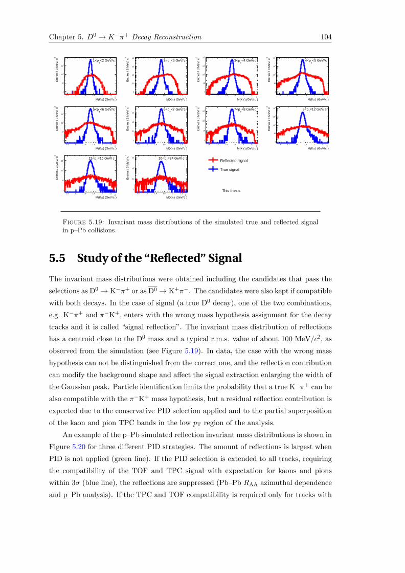
Chapter 5. D0 → K−π+ Decay Reconstruction 104
Reflected signal
True signal
This thesis
)2
c) (GeV/π(KM
1.6 1.7 1.8 1.9 2 2.1
2 cE
ntrie
s / 3
MeV
/
1
10
210
310
c<2 GeV/T
p1<
)2
c) (GeV/π(KM
1.6 1.7 1.8 1.9 2 2.1
2 cE
ntrie
s / 3
MeV
/
1
10
210
310
410
c<3 GeV/T
p2<
)2
c) (GeV/π(KM
1.6 1.7 1.8 1.9 2 2.1
2 cE
ntrie
s / 3
MeV
/
1
10
210
310
410
c<4 GeV/T
p3<
)2
c) (GeV/π(KM
1.6 1.7 1.8 1.9 2 2.1
2 cE
ntrie
s / 3
MeV
/
1
10
210
310
410
c<5 GeV/T
p4<
)2
c) (GeV/π(KM
1.6 1.7 1.8 1.9 2 2.1
2 cE
ntrie
s / 3
MeV
/
1
10
210
310
c<6 GeV/T
p5<
)2
c) (GeV/π(KM
1.6 1.7 1.8 1.9 2 2.1
2 cE
ntrie
s / 3
MeV
/
1
10
210
310
c<7 GeV/T
p6<
)2
c) (GeV/π(KM
1.6 1.7 1.8 1.9 2 2.1
2 cE
ntrie
s / 3
MeV
/
1
10
210
310
c<8 GeV/T
p7<
)2
c) (GeV/π(KM
1.6 1.7 1.8 1.9 2 2.1
2 cE
ntrie
s / 3
MeV
/
1
10
210
310
410 c<12 GeV/
Tp8<
)2
c) (GeV/π(KM
1.6 1.7 1.8 1.9 2 2.1
2 cE
ntrie
s / 3
MeV
/
1
10
210
310
c<16 GeV/T
p12<
)2
c) (GeV/π(KM
1.6 1.7 1.8 1.9 2 2.1
2 cE
ntrie
s / 3
MeV
/
1
10
210
310 c<24 GeV/
Tp16<
Figure 5.19: Invariant mass distributions of the simulated true and reflected signalin p–Pb collisions.
5.5 Study of the “Reflected” Signal
The invariant mass distributions were obtained including the candidates that pass the
selections as D0 → K−π+ or as D0 → K+π−. The candidates were also kept if compatible
with both decays. In the case of signal (a true D0 decay), one of the two combinations,
e.g. K−π+ and π−K+, enters with the wrong mass hypothesis assignment for the decay
tracks and it is called “signal reflection”. The invariant mass distribution of reflections
has a centroid close to the D0 mass and a typical r.m.s. value of about 100 MeV/c2, as
observed from the simulation (see Figure 5.19). In data, the case with the wrong mass
hypothesis can not be distinguished from the correct one, and the reflection contribution
can modify the background shape and affect the signal extraction enlarging the width of
the Gaussian peak. Particle identification limits the probability that a true K−π+ can be
also compatible with the π−K+ mass hypothesis, but a residual reflection contribution is
expected due to the conservative PID selection applied and to the partial superposition
of the kaon and pion TPC bands in the low pT region of the analysis.
An example of the p–Pb simulated reflection invariant mass distributions is shown in
Figure 5.20 for three different PID strategies. The amount of reflections is largest when
PID is not applied (green line). If the PID selection is extended to all tracks, requiring
the compatibility of the TOF and TPC signal with expectation for kaons and pions
within 3σ (blue line), the reflections are suppressed (Pb–Pb RAA azimuthal dependence
and p–Pb analysis). If the TPC and TOF compatibility is required only for tracks with
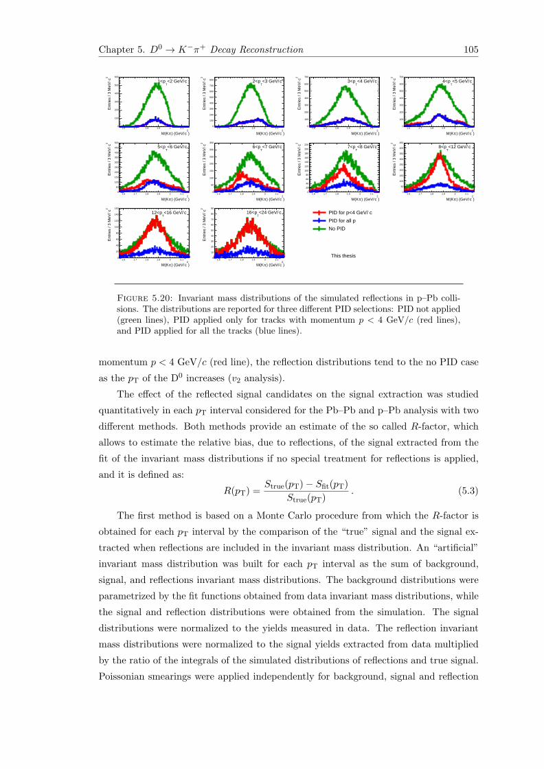
Chapter 5. D0 → K−π+ Decay Reconstruction 105
cPID for p<4 GeV/
PID for all p
No PID
This thesis
)2
c) (GeV/π(KM
1.6 1.7 1.8 1.9 2 2.1
2 cE
ntrie
s / 3
MeV
/
0
100
200
300
400
500
600
c<2 GeV/T
p1<
)2
c) (GeV/π(KM
1.6 1.7 1.8 1.9 2 2.1
2 cE
ntrie
s / 3
MeV
/
0
100
200
300
400
500
600
700
800 c<3 GeV/T
p2<
)2
c) (GeV/π(KM
1.6 1.7 1.8 1.9 2 2.1
2 cE
ntrie
s / 3
MeV
/
0
100
200
300
400
500
600
700
c<4 GeV/T
p3<
)2
c) (GeV/π(KM
1.6 1.7 1.8 1.9 2 2.1
2 cE
ntrie
s / 3
MeV
/
0
100
200
300
400
500
600
700
c<5 GeV/T
p4<
)2
c) (GeV/π(KM
1.6 1.7 1.8 1.9 2 2.1
2 cE
ntrie
s / 3
MeV
/
0
50
100
150
200
250
300
350
400
450
500
c<6 GeV/T
p5<
)2
c) (GeV/π(KM
1.6 1.7 1.8 1.9 2 2.1
2 cE
ntrie
s / 3
MeV
/
0
50
100
150
200
250
300
350
c<7 GeV/T
p6<
)2
c) (GeV/π(KM
1.6 1.7 1.8 1.9 2 2.1
2 cE
ntrie
s / 3
MeV
/
0
20
40
60
80
100
120
140
160
180
200
220c<8 GeV/
Tp7<
)2
c) (GeV/π(KM
1.6 1.7 1.8 1.9 2 2.1
2 cE
ntrie
s / 3
MeV
/
0
50
100
150
200
250
300
350
400
450
c<12 GeV/T
p8<
)2
c) (GeV/π(KM
1.6 1.7 1.8 1.9 2 2.1
2 cE
ntrie
s / 3
MeV
/
0
20
40
60
80
100
120
140
160
c<16 GeV/T
p12<
)2
c) (GeV/π(KM
1.6 1.7 1.8 1.9 2 2.1
2 cE
ntrie
s / 3
MeV
/
0
10
20
30
40
50
60
70
80
90
c<24 GeV/T
p16<
Figure 5.20: Invariant mass distributions of the simulated reflections in p–Pb colli-sions. The distributions are reported for three different PID selections: PID not applied(green lines), PID applied only for tracks with momentum p < 4 GeV/c (red lines),and PID applied for all the tracks (blue lines).
momentum p < 4 GeV/c (red line), the reflection distributions tend to the no PID case
as the pT of the D0 increases (v2 analysis).
The effect of the reflected signal candidates on the signal extraction was studied
quantitatively in each pT interval considered for the Pb–Pb and p–Pb analysis with two
different methods. Both methods provide an estimate of the so called R-factor, which
allows to estimate the relative bias, due to reflections, of the signal extracted from the
fit of the invariant mass distributions if no special treatment for reflections is applied,
and it is defined as:
R(pT) =Strue(pT)− Sfit(pT)
Strue(pT). (5.3)
The first method is based on a Monte Carlo procedure from which the R-factor is
obtained for each pT interval by the comparison of the “true” signal and the signal ex-
tracted when reflections are included in the invariant mass distribution. An “artificial”
invariant mass distribution was built for each pT interval as the sum of background,
signal, and reflections invariant mass distributions. The background distributions were
parametrized by the fit functions obtained from data invariant mass distributions, while
the signal and reflection distributions were obtained from the simulation. The signal
distributions were normalized to the yields measured in data. The reflection invariant
mass distributions were normalized to the signal yields extracted from data multiplied
by the ratio of the integrals of the simulated distributions of reflections and true signal.
Poissonian smearings were applied independently for background, signal and reflection

Chapter 5. D0 → K−π+ Decay Reconstruction 106
c GeV/T
p2 4 6 8 10 12 14 16
fac
tor
R
0.3
0.25
0.2
0.15
0.1
0.05
0
0.05
pPID for all
c<4 GeV/pPID for
No PID
This thesis
(a)
c GeV/T
p2 4 6 8 10 12 14 16 18 20 22 24
fac
tor
R
0.3
0.25
0.2
0.15
0.1
0.05
0
0.05
pPID for all
c<4 GeV/pPID for
No PID This thesis
(b)
Figure 5.21: R-factor as a function of D0 pT obtained with Monte Carlo methodfor Pb–Pb collisions in the 30–50% centrality class (a) and for minimum-bias p–Pbcollisions (b) for three PID strategies: TPC and TOF 3σ compatibility band for alltracks (blue points), for tracks with p < 4 GeV/c (red points), and PID selection notapplied.
distributions in each bin of the invariant mass distributions to simulate statistical fluctu-
ations. The signal yields were extracted applying the same fit procedure used in data and
compared with true signal injected in the invariant mass distribution. The procedure
was iterated 1000 times. The mean of the distribution of (Strue − Sfit)/Strue estimates
the R-factor. The obtained R-factors as a function of pT in Pb–Pb and p–Pb collisions
are shown in Figure 5.21 for three PID strategies. In Pb–Pb (left panel) if PID selection
is not applied (green points) the signal bias is of about 15–20% for all pT intervals, while
if the PID is applied to all the tracks the bias is within 5% up to pT = 4 GeV/c and
of about 10% from 4 to 16 GeV/c (blue points). If the PID selection is applied only
for tracks with p < 4 GeV/c (red points), the bias is similar to the case with PID for
all tracks at low pT, while it increases starting from pT = 6 GeV/c, reaching 25% at
high pT. In p–Pb (Figure 5.21(b)), a similar behaviour is observed for the three PID
strategies, but the bias stays within 5% if the PID is applied to all tracks, while reaches
at most 17% at high pT if PID is not used or an upper momentum cut is introduced in
the PID selection. The signal bias is minimum if PID is applied for all the tracks (blue
points); the residual bias is smaller in p–Pb than in Pb–Pb due to the better separation
of the kaon and pion signals in the TPC in p–Pb. The method was validated by com-
puting the R-factors without adding the reflection contributions to the invariant mass
distributions: the obtained values were compatible with zero within the uncertainties.
With the second method the R-factor was estimated directly from the data invariant
mass distributions. A template of the distribution of reflected signal candidates, which
was obtained from the simulation for each pT interval, was included in the invariant
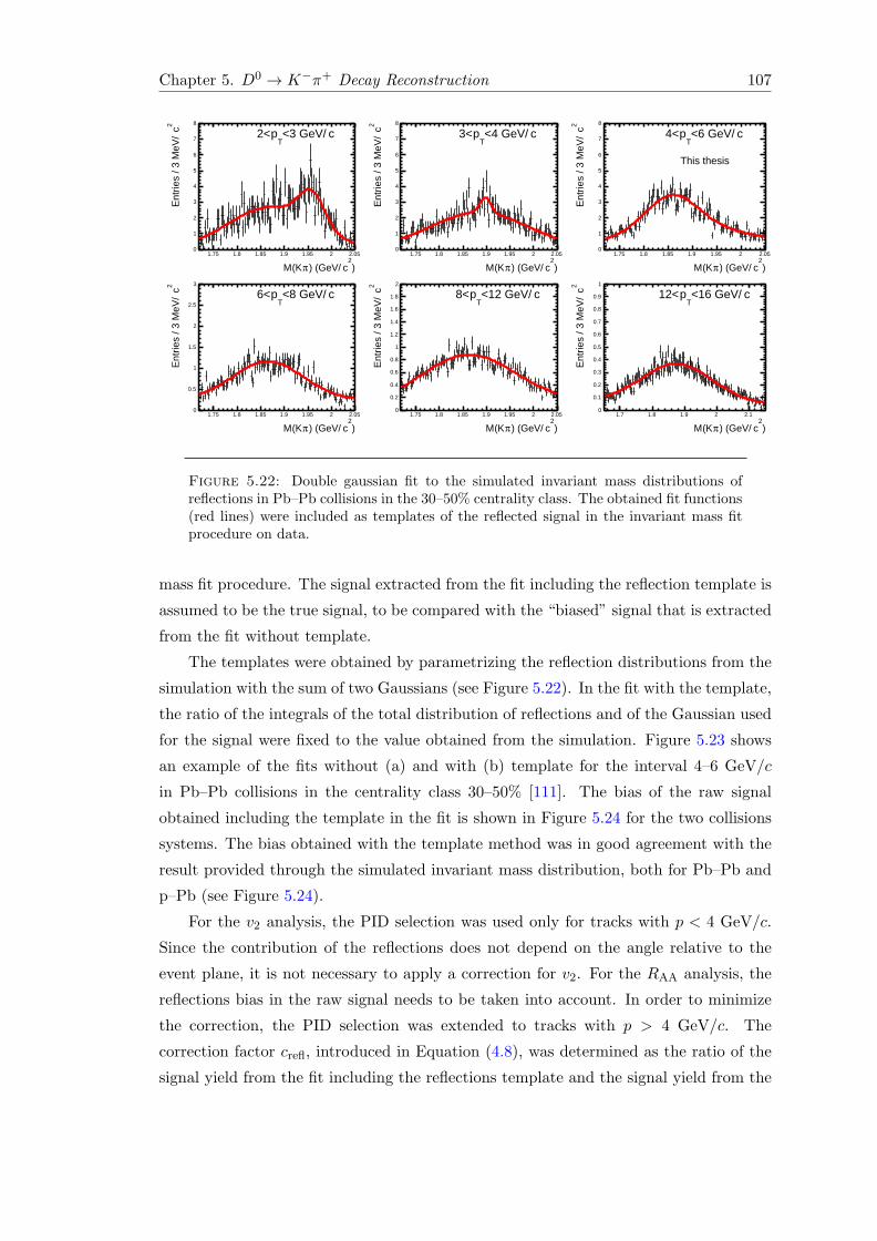
Chapter 5. D0 → K−π+ Decay Reconstruction 107
)2
c) (GeV/π(KM
1.75 1.8 1.85 1.9 1.95 2 2.05
2 cE
ntrie
s / 3
MeV
/
0
1
2
3
4
5
6
7
8
c<3 GeV/T
p2<
)2
c) (GeV/π(KM
1.75 1.8 1.85 1.9 1.95 2 2.05
2 cE
ntrie
s / 3
MeV
/
0
1
2
3
4
5
6
7
8
c<4 GeV/T
p3<
)2
c) (GeV/π(KM
1.75 1.8 1.85 1.9 1.95 2 2.05
2 cE
ntrie
s / 3
MeV
/
0
1
2
3
4
5
6
7
8
c<6 GeV/T
p4<
This thesis
)2
c) (GeV/π(KM
1.75 1.8 1.85 1.9 1.95 2 2.05
2 cE
ntrie
s / 3
MeV
/
0
0.5
1
1.5
2
2.5
3
c<8 GeV/T
p6<
)2
c) (GeV/π(KM
1.75 1.8 1.85 1.9 1.95 2 2.05
2 cE
ntrie
s / 3
MeV
/
0
0.2
0.4
0.6
0.8
1
1.2
1.4
1.6
1.8
2
c<12 GeV/T
p8<
)2
c) (GeV/π(KM
1.7 1.8 1.9 2 2.1
2 cE
ntrie
s / 3
MeV
/
0
0.1
0.2
0.3
0.4
0.5
0.6
0.7
0.8
0.9
1
c<16 GeV/T
p12<
Figure 5.22: Double gaussian fit to the simulated invariant mass distributions ofreflections in Pb–Pb collisions in the 30–50% centrality class. The obtained fit functions(red lines) were included as templates of the reflected signal in the invariant mass fitprocedure on data.
mass fit procedure. The signal extracted from the fit including the reflection template is
assumed to be the true signal, to be compared with the “biased” signal that is extracted
from the fit without template.
The templates were obtained by parametrizing the reflection distributions from the
simulation with the sum of two Gaussians (see Figure 5.22). In the fit with the template,
the ratio of the integrals of the total distribution of reflections and of the Gaussian used
for the signal were fixed to the value obtained from the simulation. Figure 5.23 shows
an example of the fits without (a) and with (b) template for the interval 4–6 GeV/c
in Pb–Pb collisions in the centrality class 30–50% [111]. The bias of the raw signal
obtained including the template in the fit is shown in Figure 5.24 for the two collisions
systems. The bias obtained with the template method was in good agreement with the
result provided through the simulated invariant mass distribution, both for Pb–Pb and
p–Pb (see Figure 5.24).
For the v2 analysis, the PID selection was used only for tracks with p < 4 GeV/c.
Since the contribution of the reflections does not depend on the angle relative to the
event plane, it is not necessary to apply a correction for v2. For the RAA analysis, the
reflections bias in the raw signal needs to be taken into account. In order to minimize
the correction, the PID selection was extended to tracks with p > 4 GeV/c. The
correction factor crefl, introduced in Equation (4.8), was determined as the ratio of the
signal yield from the fit including the reflections template and the signal yield from the
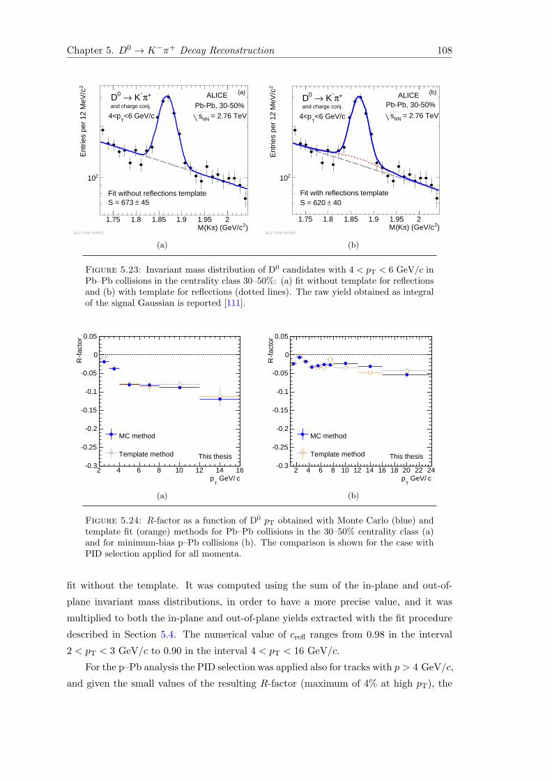
Chapter 5. D0 → K−π+ Decay Reconstruction 108
)2c) (GeV/π(KM1.75 1.8 1.85 1.9 1.95 2
2 cE
ntrie
s pe
r 12
MeV
/
210
45±S = 673 Fit without reflections template
ALICE (a)
PbPb, 3050% = 2.76 TeVNNs
+π
K→ 0D
and charge conj.
c<6 GeV/T
p4<
ALI−PUB−69961
(a)
)2c) (GeV/π(KM1.75 1.8 1.85 1.9 1.95 2
2 cE
ntrie
s pe
r 12
MeV
/
210
c<6 GeV/T
p4<
40±S = 620
+π
K→ 0D
and charge conj.
Fit with reflections template
PbPb, 3050%ALICE (b)
= 2.76 TeVNNs
ALI−PUB−69966
(b)
Figure 5.23: Invariant mass distribution of D0 candidates with 4 < pT < 6 GeV/c inPb–Pb collisions in the centrality class 30–50%: (a) fit without template for reflectionsand (b) with template for reflections (dotted lines). The raw yield obtained as integralof the signal Gaussian is reported [111].
c GeV/T
p2 4 6 8 10 12 14 16
fac
tor
R
0.3
0.25
0.2
0.15
0.1
0.05
0
0.05
MC method
Template method This thesis
(a)
c GeV/T
p2 4 6 8 10 12 14 16 18 20 22 24
fac
tor
R
0.3
0.25
0.2
0.15
0.1
0.05
0
0.05
MC method
Template method This thesis
(b)
Figure 5.24: R-factor as a function of D0 pT obtained with Monte Carlo (blue) andtemplate fit (orange) methods for Pb–Pb collisions in the 30–50% centrality class (a)and for minimum-bias p–Pb collisions (b). The comparison is shown for the case withPID selection applied for all momenta.
fit without the template. It was computed using the sum of the in-plane and out-of-
plane invariant mass distributions, in order to have a more precise value, and it was
multiplied to both the in-plane and out-of-plane yields extracted with the fit procedure
described in Section 5.4. The numerical value of crefl ranges from 0.98 in the interval
2 < pT < 3 GeV/c to 0.90 in the interval 4 < pT < 16 GeV/c.
For the p–Pb analysis the PID selection was applied also for tracks with p > 4 GeV/c,
and given the small values of the resulting R-factor (maximum of 4% at high pT), the

Chapter 5. D0 → K−π+ Decay Reconstruction 109
signal yields were not corrected for reflections, but the bias was taken into account as
an additional source of systematic uncertainty in the yield extraction (see Chapter 6).
The estimate of the bias due to reflected signal candidates was performed also for
the pp 2010 data sample. The D meson production cross section measured with this
data sample is used to obtain the RAA and RpPb pp reference (Section 4.3). The mea-
surement of the D meson cross section in pp at√s = 7 TeV was performed applying the
PID selection up to high momenta of the tracks, and the signal bias induced by reflec-
tions was estimated to be within 5% in all pT intervals, thus smaller than the systematic
uncertainties due to the extraction of the yields from the fit. When the nuclear modifi-
cation factor is computed the residual bias that is present in the p–Pb yields partially
cancels in the ratio with the pp references.
5.6 Efficiency Corrections
The raw yield extracted from the invariant mass analysis ND0
raw(pT) is only a fraction of
the total number of D0 produced in the collisions. D0 may not be reconstructed for dif-
ferent reasons, such as the limited detector acceptance, vertex and track reconstruction
inefficiencies, and selection cuts on the candidates. The total yield is derived through the
correction for the reconstruction and selection efficiency using Monte Carlo simulations.
The generated D0 → K−π+ decays are propagated along the simulation, reconstruc-
tion and analysis chain. The two latter steps are exactly the same as for data.
The efficiency correction (Acc × ε), introduced in Equations (4.8) and (4.12), is
calculated as the ratio of the number of D0 mesons after the reconstruction and selection
to the number of generated D0 for which all decay products are in the fiducial acceptance
region, |y| < yfid(pT).
Since charm production has low cross section, in the Monte Carlo sample used to
compute the efficiencies, the charm production is enhanced and D mesons are forced to
decay in the channels under study.
The simulations were configured with a detailed description of the ALICE apparatus
geometry and detector response. The simulations were tuned to reproduce the position
and width of the interaction vertex distribution, the number of active electronic channels
and the accuracy of the detector calibration, as well as their time evolution within the
Pb–Pb or p–Pb data taking periods. The generated particles were transported through
the ALICE detector using GEANT3 [114].
Pb–Pb
The HIJING v1.383 [115] generator was used to simulate Pb–Pb collisions at√sNN =
2.76 TeV, prompt and feed-down D0 meson signals were added using pp events from the

Chapter 5. D0 → K−π+ Decay Reconstruction 110
5 10 15
Effi
cien
cy×
Acc
epta
nce
310
210
110
1
0Prompt D, No PID0Prompt D
0Feeddown D
+π K→
0D = 2.76 TeV,NNsPbPb,
centrality 3050%
ALICE
)c (GeV/T
p5 10 15In
pla
ne /
Out
of
plan
e
0.95
1
1.05
1.1 0.02±Average ratio: 1.01
ALI−PUB−69942
Figure 5.25: Product of acceptance and efficiency for D0 mesons in Pb–Pb collisionsfor 30–50% centrality class (upper panel). The values for prompt (solid line) and feed-down (dotted line) D0 mesons are shown. The dashed line stands for the values obtainedwithout PID selection. The lower panel shows the ratio of the efficiencies for promptD0 in the in-plane and the out-of-plane regions used for the analysis. The ratio wasestimated using simulation samples with a difference in particle multiplicity similar tothat observed in data for the two azimuthal regions [111].
PYTHIA v6.4.21 [116] event generator with the Perugia-0 tune [117]. Each simulated pp
event contained a cc or bb pair with a D0 meson decaying into the K−π+ channel. Out
of all the particles produced in these PYTHIA pp events, only the heavy-flavour decay
products were kept and transported through the detector simulation together with the
particles produced by HIJING.
The efficiencies were evaluated from simulated events that had the same pT shape
and average charged-particle multiplicity, corresponding to the same detector occupancy,
as observed in data in the centrality class 30–50%. Figure 5.25 shows (Acc × ε) for
prompt and feed-down D0 mesons within the rapidity interval |y| < yfid. The magnitude
of (Acc × ε) increases with pT, starting from about 1% and reaching about 10–15% at

Chapter 5. D0 → K−π+ Decay Reconstruction 111
(rad)ϕ∆
0 0.5 1 1.5 2 2.5 3
trac
klet
sN
420
440
460
480
500
520
540
310×
This thesis
Figure 5.26: Distributions of the number of SPD tracklets (Ntracklets) in |η| < 1.6as a function of ∆ϕ in 30–50% Pb–Pb collisions. The in-plane and the out-of-planeregions are indicated.
high pT. The values of (Acc × ε) are also shown for the case where the PID selection
was not applied. The relative difference with respect to the (Acc × ε) obtained using
also the PID selection is about 5%, thus illustrating the high efficiency of the applied
PID strategy. The D0 mesons from B decays have larger (Acc × ε) than prompt D0’s
(by a factor of about 1.5), because the decay vertices of the feed-down D mesons are
more displaced from the primary vertex and, therefore, more efficiently selected by the
topological cuts.
A possible difference in the reconstruction and selection efficiency between in-plane
and out-of-plane D0 mesons was investigated using simulations. The difference could
arise from the variation of the particle density, and consequently of the detector occu-
pancy, induced by the azimuthal anisotropy of bulk particle production. The difference
in occupancy was estimated in data using the multiplicity of SPD tracklets, which mea-
sures the multiplicity of charged particles with pT > 50 MeV/c and |η| < 1.6, in the two
considered azimuthal regions. The SPD tracklet multiplicity in the 30–50% centrality
class was found to be larger in-plane than out-of-plane by about 12% (mean variation,
see Figure 5.26). In order to study the efficiency variation, two samples of simulated
events with 12% difference in average multiplicity were used. The ratio of the efficiencies
obtained from these two data sets was found to be consistent with unity (see lower panel
of Figure 5.25) and therefore no correction was applied.

Chapter 5. D0 → K−π+ Decay Reconstruction 112
|<1)η (|tracklets
N0 50 100 150 200
Ent
ries
0.005
0.01
0.015
0.02
MeasuredSimulated
This thesis
Figure 5.27: Distributions of the number of SPD tracklets (Ntracklets) in |η| < 1obtained from data (red) and from simulation (blue). The two distributions are nor-malized to their integral.
p–Pb
Proton–lead events were generated starting from a pp PYTHIA event with forced D
meson production (as described for the Pb–Pb case). For each event, a Ncoll value
was sampled from a minimum-bias distribution obtained from a Glauber Monte Carlo
simulation. If the sampled number of binary collisions was larger than 1, a HIJING
(v1.36 version) p–Pb event was added as underlying event.
The generated D meson pT spectrum used to calculate the efficiencies was tuned to
reproduce the shape given by FONLL calculations [34–36] at√s = 5.02 TeV, by means
of a weighting procedure of the generated spectrum. The weight function was obtained
from the ratio of the FONLL pT distribution to the generated one.
The efficiency for D meson reconstruction and selection depends also on the multi-
plicity of particles produced in the collision, mainly because the vertex reconstruction
efficiency and the resolution on the primary vertex position depend on the number of
tracks used for its evaluation. In particular, the resolution on the primary vertex im-
proves with increasing multiplicity. As a consequence, the resolution of the selection
variables that make use of the primary vertex position (track impact parameter, D me-
son decay length, pointing angle) also improves with increasing multiplicity, inducing a
multiplicity dependence in the topological selection efficiency.

Chapter 5. D0 → K−π+ Decay Reconstruction 113
)c (GeV/T
p5 10 15 20
Effi
cien
cy×
Acc
epta
nce
310
210
110
1
0Prompt D
, No PID0
Prompt D0
Feeddown D
= 5.02 TeV, min. biasNN
spPb, +
π
K→
0D
This thesis
(a)
laby
0.8 0.6 0.4 0.2 0 0.2 0.4 0.6 0.8
Effi
cien
cy×
Acc
epta
nce
310
210
110
1
0Prompt D
0Feeddown D
= 5.02 TeVNN
spPb, +
π
K→
0D
c<5 GeV/T
p2<c<8 GeV/
Tp5<
c<16 GeV/T
p8< This thesis
(b)
Figure 5.28: (a) D0 → K−π+ (Acc × ε) as a function of pT for prompt (solid line)and feed-down (dotted line) D0 in minimum-bias p–Pb collisions at
√sNN = 5.02 TeV.
The values for prompt D0 mesons obtained without PID selection (dashed line) arealso displayed. (b) Product of acceptance and efficiency as a function of rapidity forD0 mesons in p–Pb collisions. The values of (Acc × ε) for prompt (open circles) andfeed-down (filled squares) D0 are shown for three pT intervals.
The Monte Carlo multiplicity distribution was observed to be different from that
of data (see Figure 5.27), therefore the simulated distribution was tuned to reproduce
the one measured in minimum-bias p–Pb collisions. The ratio of the distributions of the
number of SPD tracklets (Ntracklets) obtained from data to that simulated was computed
for events containing at least one D0 candidate with an invariant mass compatible with
D0 mass within 20 MeV/c2. This ratio was used as a weight function applied to the
simulated events in order to reproduce the charged-particle multiplicity observed in data.
The D0 → K−π+ (Acc × ε) for prompt and feed-down D0 mesons in p–Pb collisions is
shown in Figure 5.28 as a function of pT and rapidity. As observed in the Pb–Pb
case, the (Acc× ε) increases with transverse momentum of the D0 because of the larger
displacement of the decay vertex of high-pT candidates due to the Lorentz boost. It
varies from about 1% for 1 < pT < 2 GeV/c to 40% for pT > 12 GeV/c. Similarly to the
Pb–Pb (Acc × ε), also in p–Pb the values for feed-down D0 are larger than for prompt
mesons, and the efficiency of the PID selection is of about 95%.
In the simulation it was not possible to select the centrality classes using the same
event-activity estimators considered in data because the particles produced at forward
rapidities were not transported through the detector. Therefore, a weighting procedure
was applied to obtain the (Acc × ε) factors in each event class defined with the three
estimators considered (Chapter 4). Weight functions were used to reproduce in the
simulation the multiplicity distributions measured in data for each event class. The
Ntracklets distributions at midrapidity (|η| < 1) were measured in data for each class
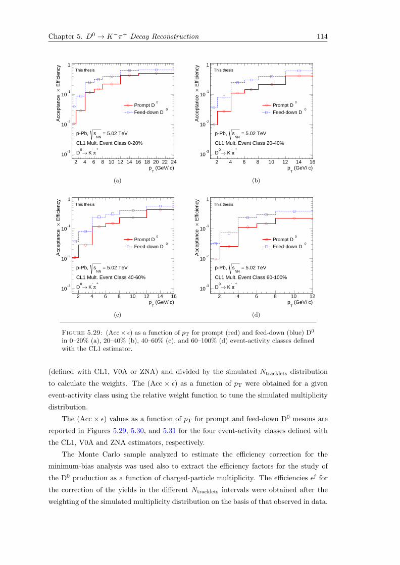
Chapter 5. D0 → K−π+ Decay Reconstruction 114
)c (GeV/T
p2 4 6 8 10 12 14 16 18 20 22 24
Effi
cien
cy×
Acc
epta
nce
310
210
110
1
0Prompt D
0Feeddown D
= 5.02 TeVNN
spPb,
CL1 Mult. Event Class 020%+
π
K→
0D
This thesis
(a)
)c (GeV/T
p2 4 6 8 10 12 14 16
Effi
cien
cy×
Acc
epta
nce
310
210
110
1
0Prompt D
0Feeddown D
= 5.02 TeVNN
spPb,
CL1 Mult. Event Class 2040%+
π
K→
0D
This thesis
(b)
)c (GeV/T
p2 4 6 8 10 12 14 16
Effi
cien
cy×
Acc
epta
nce
310
210
110
1
0Prompt D
0Feeddown D
= 5.02 TeVNN
spPb,
CL1 Mult. Event Class 4060%+
π
K→
0D
This thesis
(c)
)c (GeV/T
p2 4 6 8 10 12
Effi
cien
cy×
Acc
epta
nce
310
210
110
1
0Prompt D
0Feeddown D
= 5.02 TeVNN
spPb,
CL1 Mult. Event Class 60100%+
π
K→
0D
This thesis
(d)
Figure 5.29: (Acc× ε) as a function of pT for prompt (red) and feed-down (blue) D0
in 0–20% (a), 20–40% (b), 40–60% (c), and 60–100% (d) event-activity classes definedwith the CL1 estimator.
(defined with CL1, V0A or ZNA) and divided by the simulated Ntracklets distribution
to calculate the weights. The (Acc × ε) as a function of pT were obtained for a given
event-activity class using the relative weight function to tune the simulated multiplicity
distribution.
The (Acc× ε) values as a function of pT for prompt and feed-down D0 mesons are
reported in Figures 5.29, 5.30, and 5.31 for the four event-activity classes defined with
the CL1, V0A and ZNA estimators, respectively.
The Monte Carlo sample analyzed to estimate the efficiency correction for the
minimum-bias analysis was used also to extract the efficiency factors for the study of
the D0 production as a function of charged-particle multiplicity. The efficiencies εj for
the correction of the yields in the different Ntracklets intervals were obtained after the
weighting of the simulated multiplicity distribution on the basis of that observed in data.

Chapter 5. D0 → K−π+ Decay Reconstruction 115
)c (GeV/T
p2 4 6 8 10 12 14 16 18 20 22 24
Effi
cien
cy×
Acc
epta
nce
310
210
110
1
0Prompt D
0Feeddown D
= 5.02 TeVNN
spPb,
V0A Mult. Event Class 020%+
π
K→
0D
This thesis
(a)
)c (GeV/T
p2 4 6 8 10 12 14 16
Effi
cien
cy×
Acc
epta
nce
310
210
110
1
0Prompt D
0Feeddown D
= 5.02 TeVNN
spPb,
V0A Mult. Event Class 2040%+
π
K→
0D
This thesis
(b)
)c (GeV/T
p2 4 6 8 10 12 14 16
Effi
cien
cy×
Acc
epta
nce
310
210
110
1
0Prompt D
0Feeddown D
= 5.02 TeVNN
spPb,
V0A Mult. Event Class 4060%+
π
K→
0D
This thesis
(c)
)c (GeV/T
p2 4 6 8 10 12 14 16
Effi
cien
cy×
Acc
epta
nce
310
210
110
1
0Prompt D
0Feeddown D
= 5.02 TeVNN
spPb,
V0A Mult. Event Class 60100%+
π
K→
0D
This thesis
(d)
Figure 5.30: (Acc × ε) as a function of pT for prompt and feed-down D0 in 0–20%(a), 20–40% (b), 40–60% (c), and 60–100% (d) event-activity classes defined with theV0A estimator.
Figure 5.32(a) shows the efficiencies for prompt D0 mesons as a function of Ntracklets for
the five pT intervals considered for the analysis. The values of ε increase as a func-
tion of pT and also with increasing multiplicity, as expected. The efficiencies εj for the
correction of the yields in the different NV0A intervals were obtained by weighting the
simulated Ntracklets distribution in order to reproduce the distributions measured in data
for each NV0A interval. Figure 5.32(b) shows the efficiencies for prompt D0 mesons as a
function of NV0A for the five pT intervals considered for the analysis.

Chapter 5. D0 → K−π+ Decay Reconstruction 116
)c (GeV/T
p2 4 6 8 10 12 14 16 18 20 22 24
Effi
cien
cy×
Acc
epta
nce
310
210
110
1
0Prompt D
0Feeddown D
= 5.02 TeVNN
spPb,
ZN Energy Event Class 020%+
π
K→
0D
This thesis
(a)
)c (GeV/T
p2 4 6 8 10 12 14 16 18 20 22 24
Effi
cien
cy×
Acc
epta
nce
310
210
110
1
0Prompt D
0Feeddown D
= 5.02 TeVNN
spPb,
ZN Energy Event Class 2040%+
π
K→
0D
This thesis
(b)
)c (GeV/T
p2 4 6 8 10 12 14 16 18 20 22 24
Effi
cien
cy×
Acc
epta
nce
310
210
110
1
0Prompt D
0Feeddown D
= 5.02 TeVNN
spPb,
ZN Energy Event Class 4060%+
π
K→
0D
This thesis
(c)
)c (GeV/T
p2 4 6 8 10 12 14 16
Effi
cien
cy×
Acc
epta
nce
310
210
110
1
0Prompt D
0Feeddown D
= 5.02 TeVNN
spPb,
ZN Energy Event Class 60100%+
π
K→
0D
This thesis
(d)
Figure 5.31: (Acc × ε) as a function of pT for prompt and feed-down D0 in 0–20%(a), 20–40% (b), 40–60% (c), and 60–100% (d) event-activity classes defined with theZNA estimator.
trackletsN
20 40 60 80 100 120 140 160 180 200
Effi
cien
cy
210
110
1c<2 GeV/
Tp1<
c<4 GeV/T
p2<c<8 GeV/
Tp4<
c<12 GeV/T
p8<c<24 GeV/
Tp12<
= 5.02 TeVNN
spPb
+π
K→
0D
and charge conjugates
(a)
V0AN
100 200 300 400 500 600 700
Effi
cien
cy
210
110
1c<2 GeV/
Tp1<
c<4 GeV/T
p2<c<8 GeV/
Tp4<
c<12 GeV/T
p8<c<24 GeV/
Tp12<
= 5.02 TeVNN
spPb
+π
K→
0D
and charge conjugates
(b)
Figure 5.32: Efficiencies for prompt D0 as a function of Ntracklets (a) and NV0A (b)for the five pT intervals considered for the analysis.

Chapter 5. D0 → K−π+ Decay Reconstruction 117
5.7 Correction for Feed-Down from B Decays
The prompt D0 meson production yields dN/dpT in Pb–Pb and p–Pb collisions were
obtained by subtracting the contribution of D mesons from B decays.
The fraction fprompt of D0 coming from c quark hadronization, i.e. the correction
factor that accounts for the feed-down from B meson (see Equations (4.8) and (4.12) in
Chapter 4), was evaluated using the B production cross section from the FONLL pQCD
calculation [34–36], and the B → D0 + X kinematics from the EvtGen package [118].
The cross section for the feed-down component for the D0 was computed at the energy
of the collisions (2.76 TeV for Pb–Pb and 5.02 for p–Pb), scaled by the average nuclear
overlap function 〈TAA〉 or 〈TpA〉, and used together with the Monte Carlo acceptance
times efficiency (Acc× ε)feed−down for D mesons from B decays to compute the expected
fraction of prompt D0 in the measured yields:
fprompt = 1− ND0 feed−down raw
ND0 raw=
= 1− 〈TAA(pA)〉 ×(
d2σ
dydpT
)FONLL
feed−down
×Rfeed−downAA(pA) ×
× (Acc× ε)feed−down ·∆y∆pT · BR ·Nevt
ND0 raw/2. (5.4)
The symbol of the pT-dependence (pT) is omitted in the formulas, for brevity. The
nuclear modification factor of the feed-down D0 mesons, Rfeed−downAA(pA) , is related to the
nuclear modification of beauty production, which has not been measured in the pT
interval of the analysis.
An alternative method to obtain the prompt fraction was considered. fprompt is
computed using the FONLL cross sections for prompt and feed-down D mesons (with
B→ D +X) and their respective Monte Carlo efficiencies:
fprompt =
1 +
(Acc× ε)feed−down
(Acc× ε)prompt
dσFONLLfeed−down
dpT
∣∣∣∣|y|<0.5
dσFONLLprompt
dpT
∣∣∣∣|y|<0.5
Rfeed−downAA(pA)
RpromptAA(pA)
−1
. (5.5)
The measured raw yield is multiplied by the fprompt(pT) correction factor to obtain
the prompt D0 cross section. Since the central value of the FONLL beauty cross section
calculations describe better data at different energies and rapidities than the calculations
of charm cross section, the central value of the fprompt(pT) calculation is taken from the
first method, which does not depend on the FONLL charm calculation. The feed-down
subtraction uncertainties were defined as the envelope of the uncertainties from both
methods (see Chapter 6).

Chapter 5. D0 → K−π+ Decay Reconstruction 118
)c (GeV/T
p 2 4 6 8 10 12 14 16
prom
ptf
0
0.1
0.2
0.3
0.4
0.5
0.6
0.7
0.8
0.9
1
PbPb 3050%
(a)
)c (GeV/T
p 2 4 6 8 10 12 14 16 18 20 22 24
prom
ptf
0
0.1
0.2
0.3
0.4
0.5
0.6
0.7
0.8
0.9
1
pPb min. bias
(b)
Figure 5.33: (a) Fraction of prompt D0 mesons obtained in Pb–Pb collisions in the30–50% centrality class with the hypothesis Rfeed−down
AA = 2 · RpromptAA . (b) Fraction
of prompt D0 mesons obtained in p–Pb collisions with the hypothesis Rfeed−downpPb =
RpromptpPb . The open boxes indicate the uncertainty (see Chapter 6) obtained considering
the variation of the hypothesis and the two methods to calculate fprompt
Pb–Pb Analysis
The comparison of the nuclear modification factor of prompt D mesons with that of
J/ψ from B decays measured in the CMS experiment indicates that charmed hadrons
are more suppressed than beauty hadrons (see Section 2.3.1). Therefore, for the Pb–Pb
analysis, it was assumed that the ratio of the nuclear modification factors for feed-
down and prompt D mesons lies in the range 1 < Rfeed−downAA /Rprompt
AA < 3. The value
Rfeed−downAA = 2 · Rprompt
AA was used to compute the correction, and the variation over
the full range was used to assign a systematic uncertainty (see Chapter 6). With this
assumption, the resulting fprompt for D0 mesons ranges from about 0.86 in the lowest
transverse momentum interval (2 < pT < 3 GeV/c) to about 0.75 at high pT (Fig-
ure 5.33(a)).
The measured v2 is a combination of the v2 of promptly produced and feed-down
D0 mesons. The elliptic flow of prompt D0, vprompt2 , can be obtained from the measured
vall2 (v2{EP}) as:
vprompt2 =
1
fpromptvall
2 −1− fprompt
fpromptvfeed−down
2 , (5.6)
where vfeed−down2 is the elliptic flow of D0 mesons from B decays, which depends on the
dynamics of beauty quarks in the medium. It can be seen in Equation (5.6) that vall2
coincides with vprompt2 if vfeed−down
2 = vprompt2 , independent of fprompt. Therefore, the
assumption vfeed−down2 = vprompt
2 was used to compute the central value of the results

Chapter 5. D0 → K−π+ Decay Reconstruction 119
for the prompt D0 elliptic flow. Due to the larger mass of the b quark, the v2 of B
mesons is expected to be lower than that of D mesons. Therefore, the assumption made
to calculate the central values results to be the most conservative for the observation of
D meson v2 > 0. The variation of vfeed−down2 in the interval 0 ≤ vfeed−down
2 ≤ vprompt2
was considered to estimate the systematic uncertainty (see Chapter 6).
p–Pb Analysis
For the p–Pb analysis, the prompt fraction was calculated assuming Rfeed−downpPb =
RpromptpPb , and the ratio of the nuclear modification factors was varied in the range
0.9 < Rfeed−downpPb /Rprompt
pPb < 1.3 to evaluate the systematic uncertainty. The result-
ing fprompt is shown as a function of pT in Figure 5.33(b): it ranges from 0.9 in the
lowest pT interval (1 < pT < 2 GeV/c) to about 0.85 at higher pT. These assumptions
were based on the study of the possible modification of the B hadron production due to
initial state effects. The estimate of the influence of shadowing in the prompt and feed-
down D0 production was performed using NLO pQCD calculations (MNR [28]) including
the EPS09 nuclear modification of the parton distribution functions. The resulting nu-
clear modification factor of the prompt D and B mesons is shown in Figure 5.34(a).
The equivalent calculation of the RpPb of the D0 from B with EPS09 shadowing was
obtained considering the EvtGen decayer for the D from B decays, see Figure 5.34(b).
Their ratio is shown in Figure 5.34(c). The relative ratio is evaluated considering the
uncertainties on the prompt and feed-down D to be correlated, i.e. only central/up-
per/lower bands of the calculations are taken into account when computing the ratio,
and not their combination.
The calculation of fprompt was also performed setting the central value of the ratio
Rfeed−downpPb /Rprompt
pPb to that of the calculation reported in Figure 5.34(c), and considering
an interval of 3 times the uncertainty around the central value as range of variation of
the hypothesis. The variation of the central values of the RpPb obtained with the two
hypotheses (Rfeed−downpPb /Rprompt
pPb = 1 and Rfeed−downpPb /Rprompt
pPb as in Figure 5.34(c)) was
found to be much smaller than the systematic uncertainty, which remained very similar
as well. Therefore, the first, pT-independent, option was chosen.

Chapter 5. D0 → K−π+ Decay Reconstruction 120
(a)
(GeV/c)T
p0 5 10 15 20 25
pPb
R
0.6
0.7
0.8
0.9
1
1.1
1.2
1.3
1.4
(b)
(GeV/c)T
p0 5 10 15 20 25
pPb
R
0.6
0.7
0.8
0.9
1
1.1
1.2
1.3
1.4
(c)
Figure 5.34: (a) Calculation of the D and B meson nuclear modification factor includ-ing EPS09 shadowing. (b) Nuclear modification factor of D0 from B decays obtainedwith EvtGen decayer and including shadowing. (c) Ratio of D0 from B and prompt D0
nuclear modification factors.

6Systematic Uncertainties
This chapter is devoted to the description of the systematic uncertainties that were
studied for each observable in Pb–Pb and p–Pb collisions. The various sources of un-
certainty are listed in Table 6.1. In the first part of the chapter, the methods applied to
evaluate the “data systematics” (yield extraction, correction for reflections, tracking/-
cut/PID efficiency and Monte Carlo pT and multiplicity distributions) are presented.
The description of the systematic uncertainty related to the B feed-down subtraction
and to the scaling of the pp reference cross section needed to compute the nuclear mod-
ification factor are given in Sections 6.7 and 6.8, respectively. In the last four sections
the values of the uncertainties for each measured observable are summarized, in partic-
ular: Section 6.9 is devoted to the D0 v2 measurement, Section 6.10 to the azimuthal
dependence of the RAA, Section 6.11 to the minimum-bias measurements in p–Pb colli-
sions (namely the pT-differential cross section and RpPb and the pT- and y-differential
cross section), Section 6.12 to the multiplicity-dependent analysis carried out in p–Pb
collisions (namely the QpPb and the relative yields as a function of multiplicity).
6.1 Yield Extraction
One of the main sources of systematic uncertainty originates from the D0 yield extrac-
tion using a fit to the invariant mass distributions. This uncertainty was estimated
by repeating the fits under different conditions and by using an alternative method for
the yield determination. In general, the following variations to the fit procedure were
considered:
- different fit range;
- different function to describe the background, in particular parabolic and linear
functions were tested in addition to the exponential;
121

Chapter 6. Systematic Uncertainties 122
Table 6.1: Sources of systematic uncertainties studied for the observables that weremeasured. The X symbol indicates a source of systematics that affects and was esti-mated for that particular observable. The × indicates a source that does not contributeto the systematics for a particular observable.
Measurement v2 RAAdσ
dpT
dσdpTdy RpPb QpPb
d2ND0/dydpT
〈d2ND0/dydpT〉
Yield extraction X X X X X X X
Correction for reflections × X X X X X ×Tracking efficiency × X X X X X ×Cut efficiency × X X X X X ×PID efficiency × X X X X X ×D0 pT distribution in MC × X X X X X ×Mult. distribution in MC × × × × × X ×B feed-down yield × X X X X X X
B feed-down v2 X X × × × × ×R2 correction X X × × × × ×Normalization × X X X X X X
pp reference × X X X X X ×
- fixing the centroid and width and of the Gaussian to the values observed in simu-
lations;
- changing the invariant mass bin width of the histogram;
- using a bin counting method based on counting the entries within a 3σ interval
centred on the peak position, after subtraction of the background estimated from
a fit to the side bands; the interval considered for the bin counting procedure
was also varied in order to reduce the statistical fluctuations on the systematic
uncertainties evaluation.
The v2 analysis with the event-plane method was performed by fixing the Gaussian
centroids and widths of the in-plane and out-of-plane invariant mass distributions to the
values obtained from a fit to the ϕ-integrated distribution. Therefore, the analysis was
repeated with free Gaussian parameters in the fit instead of fixing them to the values
extracted from simulations. The systematic uncertainty due to the yield measurement
was estimated as the maximum variation of the v2 values obtained from the described
tests. It amounts to 10–20% depending on pT. For the analysis of the D0 meson RAA in-
plane and out-of-plane, the uncertainty on the yield extraction was estimated using the
ϕ-integrated invariant mass distributions, in order to reduce the statistical fluctuations.
The resulting uncertainty is 7% for 2 < pT < 8 GeV/c and 10% for 8 < pT < 16 GeV/c.
For this measurement a correction factor crefl was applied to subtract the reflection
contribution from the raw yields, as explained in Section 5.5. The systematic uncertainty

Chapter 6. Systematic Uncertainties 123
on this correction was estimated by changing by ±50% the ratio of the integral of
the reflections over the integral of the signal obtained from the simulation and used
in the invariant mass fit with the reflections template. In addition, the shape of the
)c (GeV/T
p2 4 6 8 10 12 14 16
Rat
io
0.8
0.85
0.9
0.95
1
1.05
1.1
1.15
1.2
Histo / Double gausNo template / Double gausPol3 / Double gausPol6 / Double gausGaus / Double gaus This thesis
Figure 6.1: Raw yield ratios relative to the signal yield extracted with the double-Gaussian template for the reflection contribution in Pb–Pb collisions in the 30–50%centrality class. The green points are obtained without subtracting the reflected signal,thus represent the bias on the signal. The red points are obtained using the generatedreflections distributions as templates, the orange, magenta and blue points indicatethe variation of the raw signal when the template function is varied and were used toextract the systematic uncertainty on crefl factor.
reflections templates was varied using a polynomial parametrization of the distribution
from the simulation, instead of a double-Gaussian parametrization. A single-Gaussian
parametrization and the templates obtained using the generated reflections distributions
were also tested. These variations resulted in an uncertainty of 1–2% for 2 < pT <
4 GeV/c and of 5% for 4 < pT < 16 GeV/c on the crefl factor (Figure 6.1).
For the minimum-bias p–Pb analysis the uncertainty was estimated from the ratio
between the raw yield obtained with the default fit configuration and the yield extracted
considering the variations listed above. In general, the systematic uncertainties were
determined as the best estimate of the RMS of the results trying to disentangle the
effect of statistical fluctuation and removing outliers on the basis of the quality of the
fits. In some cases the background distribution was not properly reproduced by the fit
variation, or the bin counting value was driven by the fluctuations of the background
that are found when the statistics starts to be limited.

Chapter 6. Systematic Uncertainties 124
)c (GeV/T
p2 4 6 8 10 12 14 16 18 20 22 24
ref
S/S
0.8
0.85
0.9
0.95
1
1.05
1.1
1.15
1.2
Half binningDouble binningLinear bkgPol2 bkgFit range 1Fit range 2Fit range 3Bin counting Only BkgBin counting Sig.+BkgFixed sigma This thesis
Figure 6.2: Raw yield ratios relative to the signal yield extracted with the default fitprocedure as a function of pT in p–Pb collisions. The shaded area indicates the assigneduncertainty due to yield extraction.
Figure 6.2 shows the relative ratios of the raw yields evaluated to estimate the
uncertainty on the pT-differential production cross section and the RpPb.
Figure 6.3 shows the relative raw yield ratios from which the yield extraction sys-
tematics were evaluated for the y-dependent D0 production cross section. For this study
the peak widths were fixed to the values extracted from the y-integrated invariant mass
fits. This was motivated by the fact that the simulations did not reproduce consistently
the worsening of the pT resolution from y = 0.8 to y = 0, which is due to the better
space point resolution for smaller drift lengths in the TPC and to the crossing of the
central TPC electrode.
For the QpPb analysis the yield extraction systematics were evaluated in each event-
activity class for all the three estimators applying the same strategy as for the minimum-
bias case. In Figures 6.4, 6.5, and 6.6 the results of the yield extraction studies are
reported for the four event classes considered for the analysis, defined with the CL1,
V0A, and ZNA event-activity estimators.
The systematic uncertainty from raw signal extraction on the relative yields as
expressed in Equation (4.16) was obtained by testing the different approaches listed
above to separate the signal from the combinatorial background. For this analysis, in
the various multiplicity intervals, the peak position and width were fixed to the values
obtained from the multiplicity-integrated distribution. Therefore, the case with peak

Chapter 6. Systematic Uncertainties 125
laby
0.6 0.4 0.2 0 0.2 0.4 0.6
ref
S/S
0.8
0.85
0.9
0.95
1
1.05
1.1
1.15
1.2
Half binningDouble binningLinear bkgPol2 bkgFit Rannge 1Fit Range 2Fit Range 3Bin counting Only BkgBin Counting Sig.+BkgFixed sigma This thesis
c<5 GeV/T
p2<
(a)
laby
0.8 0.6 0.4 0.2 0 0.2 0.4 0.6 0.8
ref
S/S
0.8
0.85
0.9
0.95
1
1.05
1.1
1.15
1.2
Half binningDouble binningLinear bkgPol2 bkgFit Rannge 1Fit Range 2Fit Range 3Bin counting Only BkgBin Counting Sig.+BkgFixed sigma This thesis
c<8 GeV/T
p5<
(b)
laby
0.8 0.6 0.4 0.2 0 0.2 0.4 0.6 0.8
ref
S/S
0.8
0.85
0.9
0.95
1
1.05
1.1
1.15
1.2
Half binningDouble binningLinear bkgPol2 bkgFit Rannge 1Fit Range 2Fit Range 3Bin counting Only BkgBin Counting Sig.+BkgFixed sigma This thesis
c<16 GeV/T
p8<
(c)
Figure 6.3: Raw yield ratios relative to the signal yield extracted with the defaultfit procedure as a function of ylab for 2 < pT < 5 GeV/c (a), 5 < pT < 8 GeV/c (b),and 8 < pT < 16 GeV/c (c) in p–Pb collisions. The shaded area indicates the assigneduncertainty due to yield extraction.
position and width left as free parameters in the fit was also tested. The uncertainty
was estimated from the variation of the ratio of the raw yields N jraw D0/〈Nraw D0〉, where
the same raw yield extraction method was used in the multiplicity interval j and for the
multiplicity-integrated result. The values of the ratio are reported in Figure 6.7 for the
six different Ntracklets intervals considered for the analysis and defined in Table 5.5.
The values of the ratio are reported in Figure 6.8 for the NV0A intervals considered
for the analysis and defined in Table 5.6.
The systematic uncertainty due to the reflections in the p–Pb minimum-bias yields
was estimated, as explained in Section 5.5, to be of 3% up to pT = 12 GeV/c and
4% in 12 < pT < 24 GeV/c. The reflection contribution was not subtracted from the
raw yields in any of the p–Pb analysis, but considered as a possible systematic effect

Chapter 6. Systematic Uncertainties 126
)c (GeV/T
p2 4 6 8 10 12 14 16 18 20 22 24
ref
S/S
0.8
0.85
0.9
0.95
1
1.05
1.1
1.15
1.2
Half binningDouble binningLinear bkgPol2 bkgFit range 1Fit range 2Fit range 3Bin counting Only BkgBin counting Sig.+BkgFixed sigma This thesis
CL1 Mult. Event Class 020%
(a)
)c (GeV/T
p2 4 6 8 10 12 14 16
ref
S/S
0.8
0.85
0.9
0.95
1
1.05
1.1
1.15
1.2
Half binningDouble binningLinear bkgPol2 bkgFit range 1Fit range 2Fit range 3Bin counting Only BkgBin counting Sig.+BkgFixed sigma This thesis
CL1 Mult. Event Class 2040%
(b)
)c (GeV/T
p2 4 6 8 10 12 14 16
ref
S/S
0.8
0.85
0.9
0.95
1
1.05
1.1
1.15
1.2
Half binningDouble binningLinear bkgPol2 bkgFit range 1Fit range 2Fit range 3Bin counting Only BkgBin counting Sig.+BkgFixed sigma This thesis
CL1 Mult. Event Class 4060%
(c)
)c (GeV/T
p2 4 6 8 10 12
ref
S/S
0.8
0.85
0.9
0.95
1
1.05
1.1
1.15
1.2
Half binningDouble binningLinear bkgPol2 bkgFit range 1Fit range 2Fit range 3Bin counting Only BkgBin counting Sig.+BkgFixed sigma This thesis
CL1 Mult. Event Class 60100%
(d)
Figure 6.4: Raw yield ratios relative to the signal yield extracted with the default fitprocedure as a function of pT for 0–20% (a), 20–40% (b), 40–60% (c), and 60–100% (d)event-activity classes defined with the CL1 estimator in p–Pb collisions.
and added in quadrature to the yield extraction systematics. A similar study of the
reflections effect was performed as a function of rapidity, providing similar results as
those obtained for the y-integrated analysis. Moreover, the reflections contribution is
not expected to depend on multiplicity since the PID performance is not expected to
change in the considered range. Therefore, the same values as those obtained from
the y- and multiplicity-integrated sample were considered as systematic uncertainty
due to reflections for the y-differential cross section and the QpPb. No systematics
due to reflections was considered for the analysis of the relative yields as a function of
multiplicity, since the bias from reflections is expected to cancel in the ratio of the yields.

Chapter 6. Systematic Uncertainties 127
)c (GeV/T
p2 4 6 8 10 12 14 16 18 20 22 24
ref
S/S
0.8
0.85
0.9
0.95
1
1.05
1.1
1.15
1.2
Half binningDouble binningLinear bkgPol2 bkgFit range 1Fit range 2Fit range 3Bin counting Only BkgBin counting Sig.+BkgFixed sigma
This thesis
V0A Mult. Event Class 020%
(a)
)c (GeV/T
p2 4 6 8 10 12 14 16
ref
S/S
0.8
0.85
0.9
0.95
1
1.05
1.1
1.15
1.2
Half binningDouble binningLinear bkgPol2 bkgFit range 1Fit range 2Fit range 3Bin counting Only BkgBin counting Sig.+BkgFixed sigmaThis thesis
V0A Mult. Event Class 2040%
(b)
)c (GeV/T
p2 4 6 8 10 12 14 16
ref
S/S
0.8
0.85
0.9
0.95
1
1.05
1.1
1.15
1.2
Half binningDouble binningLinear bkgPol2 bkgFit range 1Fit range 2Fit range 3Bin counting Only BkgBin counting Sig.+BkgFixed sigma This thesis
V0A Mult. Event Class 4060%
(c)
)c (GeV/T
p2 4 6 8 10 12 14 16
ref
S/S
0.8
0.85
0.9
0.95
1
1.05
1.1
1.15
1.2
Half binningDouble binningLinear bkgPol2 bkgFit range 1Fit range 2Fit range 3Bin counting Only BkgBin counting Sig.+BkgFixed sigma This thesis
V0A Mult. Event Class 60100%
(d)
Figure 6.5: Raw yield ratios relative to the signal yield extracted with the default fitprocedure as a function of pT for 0–20% (a), 20–40% (b), 40–60% (c), and 60–100% (d)event-activity classes defined with the V0A estimator in p–Pb collisions.

Chapter 6. Systematic Uncertainties 128
)c (GeV/T
p2 4 6 8 10 12 14 16 18 20 22 24
ref
S/S
0.8
0.85
0.9
0.95
1
1.05
1.1
1.15
1.2
Half binningDouble binningLinear bkgPol2 bkgFit range 1Fit range 2Fit range 3Bin counting Only BkgBin counting Sig.+BkgFixed sigma This thesis
ZNA Energy Event Class 020%
(a)
)c (GeV/T
p2 4 6 8 10 12 14 16 18 20 22 24
ref
S/S
0.8
0.85
0.9
0.95
1
1.05
1.1
1.15
1.2
Half binningDouble binningLinear bkgPol2 bkgFit range 1Fit range 2Fit range 3Bin counting Only BkgBin counting Sig.+BkgFixed sigma This thesis
ZNA Energy Event Class 2040%
(b)
)c (GeV/T
p2 4 6 8 10 12 14 16 18 20 22 24
ref
S/S
0.8
0.85
0.9
0.95
1
1.05
1.1
1.15
1.2
Half binningDouble binningLinear bkgPol2 bkgFit range 1Fit range 2Fit range 3Bin counting Only BkgBin counting Sig.+BkgFixed sigma This thesis
ZNA Energy Event Class 4060%
(c)
)c (GeV/T
p2 4 6 8 10 12 14 16
ref
S/S
0.8
0.85
0.9
0.95
1
1.05
1.1
1.15
1.2
Half binningDouble binningLinear bkgPol2 bkgFit range 1Fit range 2Fit range 3Bin counting Only BkgBin counting Sig.+BkgFixed sigma This thesis
ZNA Energy Event Class 60100%
(d)
Figure 6.6: Raw yield ratios relative to the signal yield extracted with the default fitprocedure as a function of pT for 0–20% (a), 20–40% (b), 40–60% (c), and 60–100% (d)event-activity classes defined with the ZNA estimator in p–Pb collisions.

Chapter 6. Systematic Uncertainties 129
trackletsN
10 20 30 40 50 60 70 80 90 100
)re
f/S
ref
j/S
)/(S
j(S
0.6
0.7
0.8
0.9
1
1.1
1.2
1.3
1.4
Free sigmaBin counting Only BkgBin counting Sig.+BkgLinear bkgPol2 bkgFit range 1Fit range 2Fit range 3Double binningHalf binning This thesis
c<2 GeV/T
p1<
(a)
trackletsN
20 40 60 80 100 120 140 160 180 200
)re
f/S
ref
j/S
)/(S
j(S
0.6
0.7
0.8
0.9
1
1.1
1.2
1.3
1.4
Free sigmaBin counting Only BkgBin counting Sig.+BkgLinear bkgPol2 bkgFit range 1Fit range 2Fit range 3Double binningHalf binning This thesis
c<4 GeV/T
p2<
(b)
trackletsN
20 40 60 80 100 120 140 160 180 200
)re
f/S
ref
j/S
)/(S
j(S
0.6
0.7
0.8
0.9
1
1.1
1.2
1.3
1.4
Free sigmaBin counting Only BkgBin counting Sig.+BkgLinear bkgPol2 bkgFit range 1Fit range 2Fit range 3Double binningHalf binning This thesis
c<8 GeV/T
p4<
(c)
trackletsN
20 40 60 80 100 120 140 160 180 200
)re
f/S
ref
j/S
)/(S
j(S
0.6
0.7
0.8
0.9
1
1.1
1.2
1.3
1.4
Free sigmaBin counting Only BkgBin counting Sig.+BkgLinear bkgPol2 bkgFit range 1Fit range 2Fit range 3Double binningHalf binning This thesis
c<12 GeV/T
p8<
(d)
trackletsN
10 20 30 40 50 60 70 80 90 100
)re
f/S
ref
j/S
)/(S
j(S
0.6
0.7
0.8
0.9
1
1.1
1.2
1.3
1.4
Free sigmaBin counting Only BkgBin counting Sig.+BkgLinear bkgPol2 bkgFit range 1Fit range 2Fit range 3Double binningHalf binning This thesis
c<24 GeV/T
p12<
(e)
Figure 6.7: D0 yield extraction systematics as a function of Ntracklets for the five pT
intervals considered, in p–Pb collisions. The points represent the ratio of the relativeyields extracted varying the fit procedure and the signal obtained with the standard fitprocedure.

Chapter 6. Systematic Uncertainties 130
V0AN
100 200 300 400 500 600 700
)re
f/S
ref
j/S
)/(S
j(S
0.6
0.7
0.8
0.9
1
1.1
1.2
1.3
1.4
Free sigmaBin counting Only BkgBin counting Sig.+BkgLinear bkgPol2 bkgFit range 1Fit range 2Fit range 3Double binningHalf binning This thesis
c<2 GeV/T
p1<
(a)
V0AN
100 200 300 400 500 600 700
)re
f/S
ref
j/S
)/(S
j(S
0.6
0.7
0.8
0.9
1
1.1
1.2
1.3
1.4
Free sigmaBin counting Only BkgBin counting Sig.+BkgLinear bkgPol2 bkgFit range 1Fit range 2Fit range 3Double binningHalf binning This thesis
c<4 GeV/T
p2<
(b)
V0AN
100 200 300 400 500 600 700
)re
f/S
ref
j/S
)/(S
j(S
0.6
0.7
0.8
0.9
1
1.1
1.2
1.3
1.4
Free sigmaBin counting Only BkgBin counting Sig.+BkgLinear bkgPol2 bkgFit range 1Fit range 2Fit range 3Double binningHalf binning This thesis
c<8 GeV/T
p4<
(c)
V0AN
100 200 300 400 500 600 700
)re
f/S
ref
j/S
)/(S
j(S
0.6
0.7
0.8
0.9
1
1.1
1.2
1.3
1.4
Free sigmaBin counting Only BkgBin counting Sig.+BkgLinear bkgPol2 bkgFit range 1Fit range 2Fit range 3Double binningHalf binning This thesis
c<12 GeV/T
p8<
(d)
V0AN
100 200 300 400 500 600 700
)re
f/S
ref
j/S
)/(S
j(S
0.6
0.7
0.8
0.9
1
1.1
1.2
1.3
1.4
Free sigmaBin counting Only BkgBin counting Sig.+BkgLinear bkgPol2 bkgFit range 1Fit range 2Fit range 3Double binningHalf binning This thesis
c<24 GeV/T
p12<
(e)
Figure 6.8: D0 yield extraction systematics as a function of NV0A for the five pT
intervals considered, in p–Pb collisions. The points represent the ratio of the relativeyields extracted varying the fit procedure and the signal obtained with the standard fitprocedure.
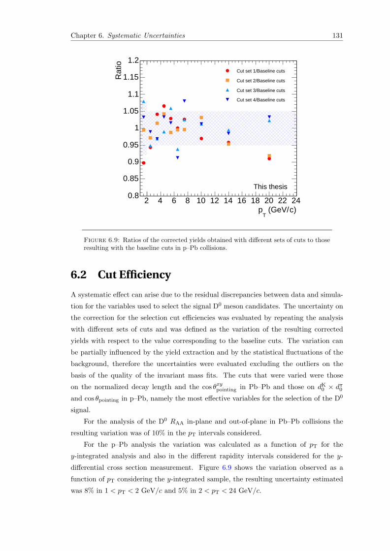
Chapter 6. Systematic Uncertainties 131
)c (GeV/T
p2 4 6 8 10 12 14 16 18 20 22 24
Rat
io
0.8
0.85
0.9
0.95
1
1.05
1.1
1.15
1.2
This thesis
Cut set 1/Baseline cuts
Cut set 2/Baseline cuts
Cut set 3/Baseline cuts
Cut set 4/Baseline cuts
Figure 6.9: Ratios of the corrected yields obtained with different sets of cuts to thoseresulting with the baseline cuts in p–Pb collisions.
6.2 Cut Efficiency
A systematic effect can arise due to the residual discrepancies between data and simula-
tion for the variables used to select the signal D0 meson candidates. The uncertainty on
the correction for the selection cut efficiencies was evaluated by repeating the analysis
with different sets of cuts and was defined as the variation of the resulting corrected
yields with respect to the value corresponding to the baseline cuts. The variation can
be partially influenced by the yield extraction and by the statistical fluctuations of the
background, therefore the uncertainties were evaluated excluding the outliers on the
basis of the quality of the invariant mass fits. The cuts that were varied were those
on the normalized decay length and the cos θxypointing in Pb–Pb and those on dK0 × dπ0
and cos θpointing in p–Pb, namely the most effective variables for the selection of the D0
signal.
For the analysis of the D0 RAA in-plane and out-of-plane in Pb–Pb collisions the
resulting variation was of 10% in the pT intervals considered.
For the p–Pb analysis the variation was calculated as a function of pT for the
y-integrated analysis and also in the different rapidity intervals considered for the y-
differential cross section measurement. Figure 6.9 shows the variation observed as a
function of pT considering the y-integrated sample, the resulting uncertainty estimated
was 8% in 1 < pT < 2 GeV/c and 5% in 2 < pT < 24 GeV/c.
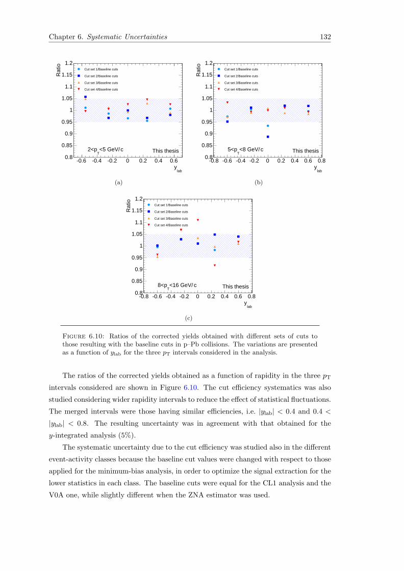
Chapter 6. Systematic Uncertainties 132
laby
0.6 0.4 0.2 0 0.2 0.4 0.6
Rat
io
0.8
0.85
0.9
0.95
1
1.05
1.1
1.15
1.2
c<5 GeV/T
p2< This thesis
Cut set 1/Baseline cuts
Cut set 2/Baseline cuts
Cut set 3/Baseline cuts
Cut set 4/Baseline cuts
(a)
laby
0.8 0.6 0.4 0.2 0 0.2 0.4 0.6 0.8
Rat
io
0.8
0.85
0.9
0.95
1
1.05
1.1
1.15
1.2
c<8 GeV/T
p5< This thesis
Cut set 1/Baseline cuts
Cut set 2/Baseline cuts
Cut set 3/Baseline cuts
Cut set 4/Baseline cuts
(b)
laby
0.8 0.6 0.4 0.2 0 0.2 0.4 0.6 0.8
Rat
io
0.8
0.85
0.9
0.95
1
1.05
1.1
1.15
1.2
c<16 GeV/T
p8< This thesis
Cut set 1/Baseline cuts
Cut set 2/Baseline cuts
Cut set 3/Baseline cuts
Cut set 4/Baseline cuts
(c)
Figure 6.10: Ratios of the corrected yields obtained with different sets of cuts tothose resulting with the baseline cuts in p–Pb collisions. The variations are presentedas a function of ylab for the three pT intervals considered in the analysis.
The ratios of the corrected yields obtained as a function of rapidity in the three pT
intervals considered are shown in Figure 6.10. The cut efficiency systematics was also
studied considering wider rapidity intervals to reduce the effect of statistical fluctuations.
The merged intervals were those having similar efficiencies, i.e. |ylab| < 0.4 and 0.4 <
|ylab| < 0.8. The resulting uncertainty was in agreement with that obtained for the
y-integrated analysis (5%).
The systematic uncertainty due to the cut efficiency was studied also in the different
event-activity classes because the baseline cut values were changed with respect to those
applied for the minimum-bias analysis, in order to optimize the signal extraction for the
lower statistics in each class. The baseline cuts were equal for the CL1 analysis and the
V0A one, while slightly different when the ZNA estimator was used.

Chapter 6. Systematic Uncertainties 133
)c (GeV/T
p2 4 6 8 10 12 14 16 18 20 22 24
Rat
io
0.6
0.7
0.8
0.9
1
1.1
1.2
1.3
1.4
V0A Mult. Event Class 020%
This thesis
Cut set 1/Baseline cuts
Cut set 2/Baseline cuts
Cut set 3/Baseline cuts
Cut set 4/Baseline cuts
(a)
)c (GeV/T
p2 4 6 8 10 12 14 16
Rat
io
0.6
0.7
0.8
0.9
1
1.1
1.2
1.3
1.4
V0A Mult. Event Class 2040%
This thesis
Cut set 1/Baseline cuts
Cut set 2/Baseline cuts
Cut set 3/Baseline cuts
Cut set 4/Baseline cuts
(b)
)c (GeV/T
p2 4 6 8 10 12 14 16
Rat
io
0.6
0.7
0.8
0.9
1
1.1
1.2
1.3
1.4
V0A Mult. Event Class 4060%
This thesis
Cut set 1/Baseline cuts
Cut set 2/Baseline cuts
Cut set 3/Baseline cuts
Cut set 4/Baseline cuts
(c)
)c (GeV/T
p2 4 6 8 10 12 14 16
Rat
io
0.6
0.7
0.8
0.9
1
1.1
1.2
1.3
1.4
V0A Mult. Event Class 60100%
This thesis
Cut set 1/Baseline cuts
Cut set 2/Baseline cuts
Cut set 3/Baseline cuts
Cut set 4/Baseline cuts
(d)
Figure 6.11: Ratios of the corrected yields obtained with different cuts to thoseobtained with the baseline cut values as a function of pT for 0–20% (a), 20–40% (b),40–60% (c), and 60–100% (d) event-activity classes defined with the V0A estimator inp–Pb collisions.
Figures 6.11 and 6.12 report the variations of the corrected yields for the four event-
activity classes defined with V0A and ZNA, respectively. The estimated uncertainty was
10% in 1 < pT < 2 GeV/c and 5% in 2 < pT < 24 GeV/c.
Also the analysis of the relative yields as a function of multiplicity was repeated
with different sets of topological selection criteria. It was verified that the relative yields
as defined in Equation (4.16) are not sensitive to this variation. This confirms that
the systematic uncertainty related to the topological selection description in the Monte
Carlo cancels in the ratio, and therefore no additional systematic uncertainty has to be
assumed.
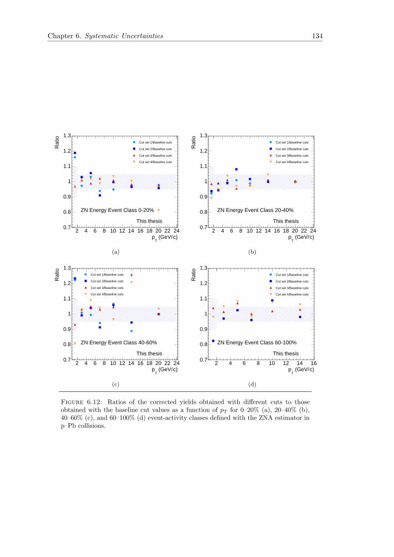
Chapter 6. Systematic Uncertainties 134
)c (GeV/T
p2 4 6 8 10 12 14 16 18 20 22 24
Rat
io
0.7
0.8
0.9
1
1.1
1.2
1.3
ZN Energy Event Class 020%
This thesis
Cut set 1/Baseline cuts
Cut set 2/Baseline cuts
Cut set 3/Baseline cuts
Cut set 4/Baseline cuts
(a)
)c (GeV/T
p2 4 6 8 10 12 14 16 18 20 22 24
Rat
io
0.7
0.8
0.9
1
1.1
1.2
1.3
ZN Energy Event Class 2040%
This thesis
Cut set 1/Baseline cuts
Cut set 2/Baseline cuts
Cut set 3/Baseline cuts
Cut set 4/Baseline cuts
(b)
)c (GeV/T
p2 4 6 8 10 12 14 16 18 20 22 24
Rat
io
0.7
0.8
0.9
1
1.1
1.2
1.3
ZN Energy Event Class 4060%
This thesis
Cut set 1/Baseline cuts
Cut set 2/Baseline cuts
Cut set 3/Baseline cuts
Cut set 4/Baseline cuts
(c)
)c (GeV/T
p2 4 6 8 10 12 14 16
Rat
io
0.7
0.8
0.9
1
1.1
1.2
1.3
ZN Energy Event Class 60100%
This thesis
Cut set 1/Baseline cuts
Cut set 2/Baseline cuts
Cut set 3/Baseline cuts
Cut set 4/Baseline cuts
(d)
Figure 6.12: Ratios of the corrected yields obtained with different cuts to thoseobtained with the baseline cut values as a function of pT for 0–20% (a), 20–40% (b),40–60% (c), and 60–100% (d) event-activity classes defined with the ZNA estimator inp–Pb collisions.

Chapter 6. Systematic Uncertainties 135
= 5.02 TeVNN
spPb,
100M events and charge conjugate
+π
K→
0D
This thesis
)2
c) (GeV/π(KM
1.75 1.8 1.85 1.9 1.95 2 2.05
2 cE
ntrie
s / 6
MeV
/
0
2000
4000
6000
8000
10000
c<2 GeV/T
p1<
0.8±) = 7.4 σSignif. (3 174±) = 1578 σS (3
59±) = 43544 σB (3
)2
c) (GeV/π(KM
1.75 1.8 1.85 1.9 1.95 2 2.05
2 cE
ntrie
s / 6
MeV
/
0
500
1000
1500
2000
2500
c<3 GeV/T
p2<
0.8±) = 16.6 σSignif. (3 102±) = 1989 σS (3
37±) = 12339 σB (3
)2
c) (GeV/π(KM
1.75 1.8 1.85 1.9 1.95 2 2.05
2 cE
ntrie
s / 6
MeV
/
0
100
200
300
400
500
600
700
800
900
1000
c<4 GeV/T
p3<
0.8±) = 19.2 σSignif. (3 66±) = 1444 σS (3 23±) = 4167 σB (3
)2
c) (GeV/π(KM
1.75 1.8 1.85 1.9 1.95 2 2.05
2 cE
ntrie
s / 6
MeV
/
0
200
400
600
800
1000
1200
1400
c<5 GeV/T
p4<
0.8±) = 19.0 σSignif. (3 80±) = 1730 σS (3 30±) = 6489 σB (3
)2
c) (GeV/π(KM
1.75 1.8 1.85 1.9 1.95 2 2.05
2 cE
ntrie
s / 6
MeV
/
0
100
200
300
400
500
600
700
c<6 GeV/T
p5<
0.8±) = 16.7 σSignif. (3 56±) = 1055 σS (3 20±) = 2904 σB (3
)2
c) (GeV/π(KM
1.75 1.8 1.85 1.9 1.95 2 2.05
2 cE
ntrie
s / 6
MeV
/0
50
100
150
200
250
300
c<7 GeV/T
p6<
0.8±) = 14.7 σSignif. (3 41±) = 667 σS (3 15±) = 1385 σB (3
)2
c) (GeV/π(KM
1.75 1.8 1.85 1.9 1.95 2
2 cE
ntrie
s / 1
5 M
eV/
0
50
100
150
200
250
300
c<8 GeV/T
p7<
0.7±) = 10.3 σSignif. (3 26±) = 300 σS (3 9±) = 552 σB (3
)2
c) (GeV/π(KM
1.7 1.75 1.8 1.85 1.9 1.95 2 2.05 2.1
2 cE
ntrie
s / 1
5 M
eV/
0
100
200
300
400
500
600
c<12 GeV/T
p8<
0.7±) = 16.9 σSignif. (3 39±) = 737 σS (3 15±) = 1161 σB (3
)2
c) (GeV/π(KM
1.7 1.75 1.8 1.85 1.9 1.95 2 2.05 2.1
2 cE
ntrie
s / 1
5 M
eV/
0
50
100
150
200
250
300
c<16 GeV/T
p12<
0.8±) = 8.6 σSignif. (3 31±) = 304 σS (3 16±) = 928 σB (3
)2
c) (GeV/π(KM
1.7 1.75 1.8 1.85 1.9 1.95 2 2.05 2.1
2 cE
ntrie
s / 2
4 M
eV/
0
20
40
60
80
100
120
140
160
180
c<24 GeV/T
p16<
0.8±) = 4.6 σSignif. (3 22±) = 114 σS (3 13±) = 495 σB (3
Figure 6.13: Distributions of the invariant mass for D0 in p–Pb collisions obtainedwithout applying PID selection. The raw signals include the reflection contribution.
6.3 PID Efficiency
The uncertainty arising from the PID selection was estimated by comparing the corrected
yields obtained with and without this selection. In both cases, the bias on the raw signal
induced by reflections was calculated and taken into account.
In Pb–Pb, the corrected yields resulting without PID selection were found to be
consistent within 5% with those obtained with the PID selection. Therefore, a systematic
uncertainty of 5% was assigned for the PID efficiency correction in the simulation.
In p–Pb, the difference between the corrected yields obtained with and without
PID selection was negligible and, thus, no uncertainty was assigned. Figure 6.13 shows
the invariant mass distributions obtained in minimum-bias p–Pb collisions when PID
selection is not applied. In this case, the background is larger with respect to the case
with PID selection applied.
For the relative yields as a function of multiplicity in p–Pb, no multiplicity-dependent
influence of the PID is expected. The TPC response is stable up to an occupancy of
300–400 tracks, so there is no expected variation of the response in the range of mul-
tiplicity considered in this analysis. For what concerns the TOF information, a small
effect on the resolution and start time information could be expected. Increasing the
event multiplicity, the fraction of events with TOF or T0 start time changes, and the
TOF PID resolution is slightly better. However, the efficiency is expected to remain
unchanged.

Chapter 6. Systematic Uncertainties 136
)c (GeV/T
p2 4 6 8 10 12 14 16 18 20 22 24
Rat
io
0.9
0.92
0.94
0.96
0.98
1
1.02
1.04
1.06
1.08
1.1
This thesis
weightsT
p weights / FONLL 5 TeV T
pNo
weightsT
p weights / FONLL 5 TeV T
pFONLL 7 TeV
Figure 6.14: Rapidity integrated efficiencies ratios as a function of pT calculated toestimate the systematic uncertainty due to the simulated D0 momentum distributionin p–Pb collisions.
6.4 Monte Carlo pT Shape
The uncertainty on the efficiencies arising from the difference between the real and
simulated D0 meson momentum distributions depends on the width of the pT intervals
and on the variation of the efficiencies within them.
The mean efficiency in a given pT interval in Pb–Pb collisions was computed by
re-weighting the simulated D0 meson yield according to the pT distribution measured
for D0 mesons in central Pb–Pb collisions [63]. The systematic uncertainty was defined
as the difference with respect to the efficiency computed using the pT distribution from
a FONLL calculation multiplied by the RAA value from one of the models that closely
describe the central value of the measurement [119–121]. This uncertainty is of 2% in
the interval 2 < pT < 3 GeV/c, where the efficiency increases steeply with pT (see
Figure 5.25), and below 1% for pT > 3 GeV/c.
The efficiency correction in p–Pb was obtained considering as pT distribution of
generated D0 mesons the one calculated with FONLL at√s = 5.02 TeV. The systematic
uncertainty was evaluated from the variation of the Monte Carlo efficiencies with respect
to those obtained without re-weighting the simulated pT distribution, and those resulting
when a weight function obtained by considering the pT distribution from FONLL at√s = 7 TeV was used.

Chapter 6. Systematic Uncertainties 137
laby
0.6 0.4 0.2 0 0.2 0.4 0.6
Rat
io
0.8
0.85
0.9
0.95
1
1.05
1.1
1.15
1.2
This thesis
c<5 GeV/T
p2<
weightsT
p weights / FONLL 5 TeV T
pNo
weightsT
p weights / FONLL 5 TeV T
pFONLL 7 TeV
(a)
laby
0.8 0.6 0.4 0.2 0 0.2 0.4 0.6 0.8
Rat
io
0.8
0.85
0.9
0.95
1
1.05
1.1
1.15
1.2
This thesis
c<8 GeV/T
p5<
weightsT
p weights / FONLL 5 TeV T
pNo
weightsT
p weights / FONLL 5 TeV T
pFONLL 7 TeV
(b)
laby
0.8 0.6 0.4 0.2 0 0.2 0.4 0.6 0.8
Rat
io
0.8
0.85
0.9
0.95
1
1.05
1.1
1.15
1.2
This thesis
c<16 GeV/T
p8<
weightsT
p weights / FONLL 5 TeV T
pNo
weightsT
p weights / FONLL 5 TeV T
pFONLL 7 TeV
(c)
Figure 6.15: Efficiencies ratios as a function of ylab for 2 < pT < 5 GeV/c (a), 5 <pT < 8 GeV/c (b), and 8 < pT < 16 GeV/c (c) calculated to estimate the systematicuncertainty due to the simulated D0 momentum distribution in p–Pb collisions.
For the y-integrated analysis the uncertainty is of 2% in 1 < pT < 2 GeV/c where the
efficiencies increase steeply with pT, and negligible in 2 < pT < 24 GeV/c (Figure 6.14).
When larger pT intervals are considered, e.g. for the cross section as a function of
rapidity, the uncertainties are larger: 8% in 2 < pT < 5 GeV/c, 2% in 5 < pT < 8 GeV/c,
and 5% in 8 < pT < 16 GeV/c (Figure 6.15).
This systematic effect was verified to be negligible in the analysis of the relative
yields as a function of multiplicity, since it cancels in the ratio of the corrected yields.
6.5 Monte Carlo Multiplicity Distribution
A systematic uncertainty due to the weighting procedure applied to obtain the (Acc ×ε) factors in each event-activity class in p–Pb collisions, defined with the CL1, V0A,
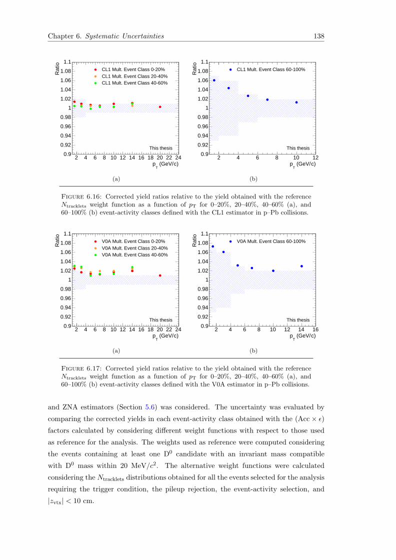
Chapter 6. Systematic Uncertainties 138
)c (GeV/T
p2 4 6 8 10 12 14 16 18 20 22 24
Rat
io
0.9
0.92
0.94
0.96
0.98
1
1.02
1.04
1.06
1.08
1.1
This thesis
CL1 Mult. Event Class 020%CL1 Mult. Event Class 2040%CL1 Mult. Event Class 4060%
(a)
)c (GeV/T
p2 4 6 8 10 12
Rat
io
0.9
0.92
0.94
0.96
0.98
1
1.02
1.04
1.06
1.08
1.1
This thesis
CL1 Mult. Event Class 60100%
(b)
Figure 6.16: Corrected yield ratios relative to the yield obtained with the referenceNtracklets weight function as a function of pT for 0–20%, 20–40%, 40–60% (a), and60–100% (b) event-activity classes defined with the CL1 estimator in p–Pb collisions.
)c (GeV/T
p2 4 6 8 10 12 14 16 18 20 22 24
Rat
io
0.9
0.92
0.94
0.96
0.98
1
1.02
1.04
1.06
1.08
1.1
This thesis
V0A Mult. Event Class 020%V0A Mult. Event Class 2040%V0A Mult. Event Class 4060%
(a)
)c (GeV/T
p2 4 6 8 10 12 14 16
Rat
io
0.9
0.92
0.94
0.96
0.98
1
1.02
1.04
1.06
1.08
1.1
This thesis
V0A Mult. Event Class 60100%
(b)
Figure 6.17: Corrected yield ratios relative to the yield obtained with the referenceNtracklets weight function as a function of pT for 0–20%, 20–40%, 40–60% (a), and60–100% (b) event-activity classes defined with the V0A estimator in p–Pb collisions.
and ZNA estimators (Section 5.6) was considered. The uncertainty was evaluated by
comparing the corrected yields in each event-activity class obtained with the (Acc× ε)factors calculated by considering different weight functions with respect to those used
as reference for the analysis. The weights used as reference were computed considering
the events containing at least one D0 candidate with an invariant mass compatible
with D0 mass within 20 MeV/c2. The alternative weight functions were calculated
considering the Ntracklets distributions obtained for all the events selected for the analysis
requiring the trigger condition, the pileup rejection, the event-activity selection, and
|zvtx| < 10 cm.
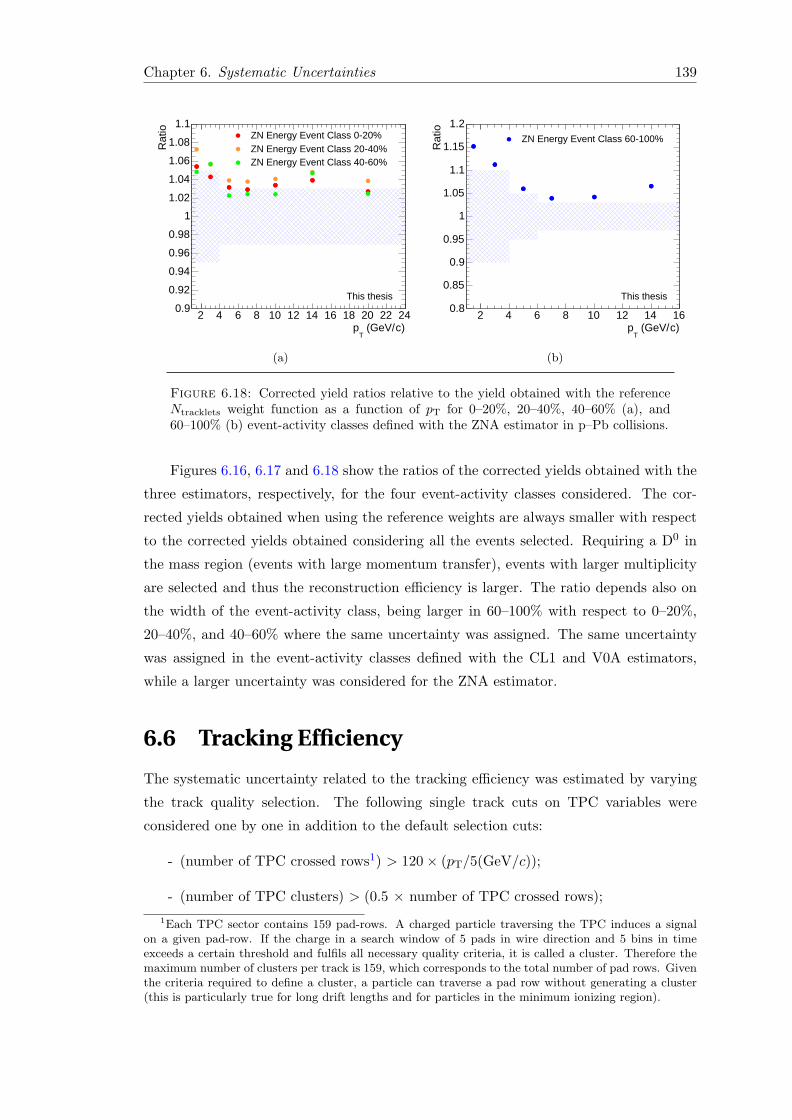
Chapter 6. Systematic Uncertainties 139
)c (GeV/T
p2 4 6 8 10 12 14 16 18 20 22 24
Rat
io
0.9
0.92
0.94
0.96
0.98
1
1.02
1.04
1.06
1.08
1.1
This thesis
ZN Energy Event Class 020%ZN Energy Event Class 2040%ZN Energy Event Class 4060%
(a)
)c (GeV/T
p2 4 6 8 10 12 14 16
Rat
io
0.8
0.85
0.9
0.95
1
1.05
1.1
1.15
1.2
This thesis
ZN Energy Event Class 60100%
(b)
Figure 6.18: Corrected yield ratios relative to the yield obtained with the referenceNtracklets weight function as a function of pT for 0–20%, 20–40%, 40–60% (a), and60–100% (b) event-activity classes defined with the ZNA estimator in p–Pb collisions.
Figures 6.16, 6.17 and 6.18 show the ratios of the corrected yields obtained with the
three estimators, respectively, for the four event-activity classes considered. The cor-
rected yields obtained when using the reference weights are always smaller with respect
to the corrected yields obtained considering all the events selected. Requiring a D0 in
the mass region (events with large momentum transfer), events with larger multiplicity
are selected and thus the reconstruction efficiency is larger. The ratio depends also on
the width of the event-activity class, being larger in 60–100% with respect to 0–20%,
20–40%, and 40–60% where the same uncertainty was assigned. The same uncertainty
was assigned in the event-activity classes defined with the CL1 and V0A estimators,
while a larger uncertainty was considered for the ZNA estimator.
6.6 Tracking Efficiency
The systematic uncertainty related to the tracking efficiency was estimated by varying
the track quality selection. The following single track cuts on TPC variables were
considered one by one in addition to the default selection cuts:
- (number of TPC crossed rows1) > 120× (pT/5(GeV/c));
- (number of TPC clusters) > (0.5 × number of TPC crossed rows);
1Each TPC sector contains 159 pad-rows. A charged particle traversing the TPC induces a signalon a given pad-row. If the charge in a search window of 5 pads in wire direction and 5 bins in timeexceeds a certain threshold and fulfils all necessary quality criteria, it is called a cluster. Therefore themaximum number of clusters per track is 159, which corresponds to the total number of pad rows. Giventhe criteria required to define a cluster, a particle can traverse a pad row without generating a cluster(this is particularly true for long drift lengths and for particles in the minimum ionizing region).

Chapter 6. Systematic Uncertainties 140
c GeV/T
p2 4 6 8 10 12 14 16
Rat
io
0.7
0.8
0.9
1
1.1
1.2
1.3N. cross. rows cut / Default cuts
N. clusters cut / Default cuts
N. clusters PID cut / Default cuts
N. clusters/N. cross. rows / Default cuts
This thesis
= 2.76 TeVNN
sPbPb
(a)
c GeV/T
p2 4 6 8 10 12 14 16 18 20 22 24
Rat
io
0.7
0.8
0.9
1
1.1
1.2
1.3N. cross. rows cut / Default cuts
N. clusters cut / Default cuts
N. clusters PID cut / Default cuts
N. clusters/N. cross. rows cut / Default cuts
This thesis
= 5.02 TeVNN
spPb
(b)
Figure 6.19: Ratio of the corrected yields obtained when applying different singletrack quality cuts to those obtained with default cuts for 30–50% Pb–Pb (a) and p–Pbcollisions (b).
- (number of TPC clusters used for PID) > (0.5 × number of TPC crossed rows);
- (number of TPC crossed rows)/(number of TPC findable clusters2) > 0.9.
The value of the systematic uncertainty was evaluated from the ratios of the corrected
pT distributions, computed with respect to the default track quality selection.
Figure 6.19 reports the ratios of the corrected yields. For Pb–Pb collisions the
maximum observed deviation is of about 10% (Figure 6.19(a)). The resulting uncertainty
was estimated to be 5% per decay track. In p–Pb collisions the assigned uncertainty was
3% per decay track on the basis of the values of the ratios obtained up to pT = 16 GeV/c
(Figure 6.19(b)).
The tracking efficiency systematic uncertainty affects the RAA in-plane and out-of-
plane, the production cross section, RpPb and QpPb measurements. In the RAA, RpPb
and QpPb measurements the tracking efficiency systematic uncertainty does not cancel
in the ratio because the yields are obtained from different data samples, namely Pb–Pb,
p–Pb and pp, where the tracking performance was different. The tracking efficiency
systematic uncertainty does not affect the v2 and the relative yields, since it cancels in
ratios of yields from the same data sample.
2The number of findable clusters is the number of geometrically possible clusters which can be assignedto a track. It takes into account the inactive zones due to chamber boundaries or the limited η-acceptancein which clusters are not findable.

Chapter 6. Systematic Uncertainties 141
6.7 Feed-down Correction
The systematic uncertainty arising from the subtraction of feed-down D0 mesons has two
contributions. The first contribution is due to the FONLL perturbative calculation of
the cross sections and it was evaluated by varying the parameters of the calculation. The
factorization and renormalization scales, µF and µR, were varied around their central
values of µF = µR = mT =√p2
T +m2c over the range 0.5 ≤ µR,F/mT ≤ 2, with the
constraint 0.5 ≤ µR/µF ≤ 2. The charm quark mass was varied within the range 1.3 ≤mc ≤ 1.7 GeV/c2, with a central value of 1.5 GeV/c2, and the beauty quark mass was
varied within the range 4.5 ≤ mb ≤ 5 GeV/c2, with a central value of 4.75 GeV/c2 [36].
fprompt was calculated with both methods introduced in Section 5.7 and the full envelope
of the uncertainty bands from the two methods obtained when varying the FONLL
parameters was taken as a systematic uncertainty. This contribution partly cancels in
the nuclear modification factor ratio, because these variations are done simultaneously
for the Pb–Pb (p–Pb) yield and for the pp reference cross section.
The prompt fraction depends explicitly also on the ratio of nuclear modification fac-
tors of feed-down and prompt D mesons. The uncertainty introduced by the hypothesis
on the value of the feed-down D meson RAA was estimated from the variation of the
ratio Rfeed−downAA /Rprompt
AA in a given range.
The central values for the prompt D0 elliptic flow, vprompt2 , were obtained assuming
vfeed−down2 = vprompt
2 (see Section 5.7). The systematic uncertainty associated with this
assumption on vfeed−down2 was estimated by varying it in the interval 0 ≤ vfeed−down
2 ≤vprompt
2 . Considering this interval vprompt2 ranges from vall
2 to vall2 /fprompt. For each
pT bin, a set of fprompt values was computed by varying the heavy-quark masses and
the perturbative scales in the FONLL calculation as indicated at the beginning of the
section, and the ratio Rfeed−downAA /Rprompt
AA in the range 1 < Rfeed−downAA /Rprompt
AA < 3,
based on the difference of the measured nuclear modification factor of prompt D meson
to that of J/ψ from B decays. The smallest value of fprompt was used to assign the
uncertainty related to the B feed-down contribution to the elliptic flow of prompt D0.
The maximum relative uncertainty was about +45−0 %.
For the RAA azimuthal dependence analysis in Pb–Pb collisions, the systematic
uncertainty due to feed-down correction was obtained varying the hypothesis on the ratio
Rfeed−downAA /Rprompt
AA in the range 1 < Rfeed−downAA /Rprompt
AA < 3. The total uncertainty due
to feed-down correction, which is in common to the in-plane and out-of-plane RAA,
ranges between +9−13% at low pT and +14
−12% at high pT. The hypothesis on the value of
v2 for D0 mesons from B decays (0 ≤ vfeed−down2 ≤ vprompt
2 ) introduces an additional
contribution to the systematic uncertainty, which is anti-correlated between Rin−planeAA

Chapter 6. Systematic Uncertainties 142
and Rout−of−planeAA . This uncertainty is typically of +5
−0% for the in-plane and +0−5% for the
out-of-plane RAA.
For the p–Pb analysis, the considered range was 0.9 < Rfeed−downpPb /Rprompt
pPb < 1.3
taking into account the possible effect of shadowing on the prompt and feed-down D
mesons nuclear modification factors (see Figure 5.34). The FONLL rapidity trend was
evaluated to be flat within 4% in the rapidity range considered for the analysis (|y| <0.8). Since further modifications of the rapidity shape due to shadowing or other cold
nuclear matter effects are considered by the B meson nuclear modification hypothesis,
no additional uncertainty to this trend was considered. The overall uncertainty due to
feed-down subtraction was +5−47% in 1 < pT < 2 GeV/c and +4
−9% in 16 < pT < 24 GeV/c
on the cross section as a function of pT, +1−7% in 1 < pT < 2 GeV/c and +4
−11% in
16 < pT < 24 GeV/c on the RpPb, and of about +5−20% in 2 < pT < 5 GeV/c, +5
−12% in
5 < pT < 8 GeV/c, and +5−10% in 8 < pT < 16 GeV/c on the cross section as function of
rapidity. The QpPb uncertainties due to feed-down correction were evaluated considering
the same procedure adopted for the minimum-bias analysis. The resulting uncertainties
are, for example, +1−7% and +1
−5% in 1 < pT < 2 GeV/c in the 0–20% and 60–100%
event-activity classes defined with the ZNA estimator, respectively.
The relative yields expressed as in Equation (4.16) assume that the relative con-
tribution of B decays to the D yields in the different multiplicity intervals is constant
and equal to that of the multiplicity integrated sample. With this assumption, fprompt
cancels in the ratio between the yield in a given multiplicity interval and that in the
multiplicity integrated sample. However, the dependence of B hadrons and prompt D
mesons with the charged-particle multiplicity could differ. In order to evaluate a sys-
tematic uncertainty due to this effect, a variation of the relative fraction of B/D hadrons
with charged-particle multiplicity was considered. The fprompt was calculated with the
two methods for the multiplicity-integrated sample, then the fraction of the yield com-
ing from B feed-down was computed as fB = 1 − fprompt. In each multiplicity interval
fB was varied by a factor increasing from 0.5 to 2 as a function of multiplicity, which
parametrizes the variation of the B/D ratio, and a set of fprompt was obtained using the
relation fprompt = 1 − fB. The range of fprompt was then converted in the uncertainty
on the relative yields, in a given multiplicity interval j, by computing f jprompt/〈fprompt〉.The systematic uncertainties due to feed-down from B decays ranges from −20% to
+10% depending on multiplicity interval.
6.8 Proton–Proton Reference
The uncertainty of the pp reference used for the calculation of the nuclear modification
factors has two contributions.

Chapter 6. Systematic Uncertainties 143
)c (GeV/T
p2 4 6 8 10 12 14 16 18 20 22 24
(7
TeV
)σ
(5.
02 T
eV)/
σ
0.5
0.6
0.7
0.8
0.9
1
1.1
1.2
0µ/
Rµ
0µ/
Fµ
1 1
0.5 0.5
2 2
2 1
1 2
1 0.5
0.5 1
scaling (5.02 TeV / 7 TeV)0
D
(a)
)c (GeV/T
p2 4 6 8 10 12 14 16 18 20 22 24
Rel
ativ
e un
cert
aint
y
0.1
0.05
0
0.05
0.1
0.15
0.2
scaling (5.02 TeV / 7 TeV)0
D
(b)
)c (GeV/T
p2 4 6 8 10 12 14 16
(7
TeV
)σ
(2.
76 T
eV)/
σ
0.2
0.3
0.4
0.5
0.6
0.7
0.8
0µ/
Rµ
0µ/
Fµ
1 1
0.5 0.5
2 2
2 1
1 2
1 0.5
0.5 1
scaling (2.76 TeV / 7 TeV)0
D
(c)
)c (GeV/T
p2 4 6 8 10 12 14 16
Rel
ativ
e un
cert
aint
y
0.2
0.1
0
0.1
0.2
0.3
0.4
scaling (2.76 TeV / 7 TeV)0
D
(d)
Figure 6.20: FONLL scaling factor from 7 TeV to 5.02 TeV (a) and its relativeuncertainty (b), and from 7 TeV to 2.76 TeV (c) and its relative uncertainty (d).
The first is due to the systematic uncertainty of the measured D0 meson pT-differential
cross section at√s = 7 TeV, which is of about 17%, approximately independent of
pT [38].
The second contribution is due to the scaling to√s = 2.76 TeV or
√s = 5.02 TeV.
The scaling factors were obtained as explained in Section 4.3 from the ratio of the
theoretical cross sections calculated at different energies. The uncertainty due to the
scaling was determined by the envelope of the scaling factors obtained by varying the
parameters of the FONLL calculation as described in Section 6.7.
The scaling factor from 7 TeV to 5.02 TeV and from 7 TeV to 2.76 TeV, and their
associated uncertainty are shown in Figure 6.20. The uncertainty on the scaling factor
ranges from +31−10% at low pT to about 5% at high pT for the Pb–Pb collision energy and
from +17.5−4 % at pT = 1 GeV/c to about 3% for pT > 8 GeV/c for the p–Pb collision
energy.

Chapter 6. Systematic Uncertainties 144
Table 6.2: Systematic uncertainties on the D0 v2 measurement in the 0–10%, 10–30%and 30–50% centrality classes for the interval 4 < pT < 6 GeV/c.
Centrality class 0–10% 10–30% 30–50%
Yield extraction 37% 22% 9%
2 or 3 sub-ev. R2 6.9% 2% 2.3%
R2 centrality dependence 2% 0.5% 2%
Total (excl. B feed-down) 38% 22% 9%
B feed-down +50−0 % +45
−0 % +48−0 %
In the interval 1 < pT < 2 GeV/c, the overall uncertainty on the cross section at√s = 5.02 TeV obtained by scaling the 2.76 TeV and the 7 TeV pp measurements were
similar. The pp reference for this pT interval was evaluated as the weighted average of
these two results, considering their relative statistical and systematic uncertainties as
weights. The uncertainty on the weighted average was obtained by propagating all the
uncertainty sources.
6.9 Summary of Uncertainties on v2
The observed v2 was corrected for the event-plane resolution (Equation (4.6)). The
uncertainty on the resolution correction factor R2 was estimated with the two and three
sub-event methods with an η-gap. The three sub-events were defined using the TPC
tracks and the signals in the two VZERO detectors. The R2 values estimated with
these two methods differ by 2.3% in the 30–50% centrality class (see Figure 5.1(b)).
A symmetric uncertainty equal to the relative difference between R2 values obtained
with the two and three sub-event methods was assigned to the D0 v2. The uncertainty
due to the centrality dependence of the event-plane resolution was estimated from the
difference between two ways to define the average resolution in the centrality class used in
the analysis, starting from the resolutions in fine centrality intervals (see Figure 5.1(b)).
The two ways considered were a plain arithmetic average and an average weighted with
the D meson yield measured in smaller centrality classes (2.5% wide). The latter was
estimated using D0 meson raw yields in wide pT intervals and the sum of the two
∆ϕ intervals, in order to reduce statistical fluctuations. The difference between these
averages was found to be about 2% for the 30–50% centrality class. The resulting total
uncertainty on R2 amounts to 3%.
Table 6.2 reports a summary of the systematic uncertainties assigned to the D0 v2
measurement with the event-plane method in the interval 4 < pT < 6 GeV/c. The
uncertainties are comparable in the other pT intervals.

Chapter 6. Systematic Uncertainties 145
6.10 Summary of Uncertainties on RAA In- and Out-
Of-Plane
The D0 yields in the two azimuthal regions with respect to the event plane, obtained from
Equation (4.8), were corrected for the event-plane resolution using the correction factor
R2 (Section 5.2) and the relation given in Equation (4.6). For example, the correction
factor for the in-plane RAA is (1 +R−12 )/2 + (Nout/N in)(1−R−1
2 )/2, where the N in(out)
is the D0 raw yield. The value R2 = (0.8059±0.001) for the 30–50% centrality class and
the typical Nout/N in magnitude result in a correction of approximately +4(−6)% for
the in-plane (out-of-plane) yields. The uncertainty of 3% on the event-plane resolution
correction factor R2 in the 30–50% centrality class was also propagated to the RAA
observable, resulting in an uncertainty in the range 0.5–2%, depending on the pT interval.
The uncertainties on the pp cross section normalization (3.5%) [38] and the average
nuclear overlap function 〈TAA〉 (4.7%) were also included [16]. The contribution due to
the 1.1% relative uncertainty on the fraction of the hadronic cross section used in the
Glauber fit to determine the centrality class was obtained by estimating the variation
of the D meson dN/dpT when the limits of the centrality classes are shifted by ±1.1%.
The resulting uncertainty, common to all pT intervals, is 2% for the 30–50% centrality
class. The total normalization uncertainty, computed as the quadratic sum of these
three contributions, is 6.2%.
The systematic uncertainties of RAA described in the previous sections were grouped
in three categories, depending on their correlation between the in-plane and the out-of-
plane measurements. The uncorrelated systematic uncertainties affect the two RAA
independently: this category includes only the yield extraction uncertainty. The corre-
lated systematic uncertainties affect the two RAA in the same way and do not change
their relative difference. The uncertainties on the efficiency corrections (for track recon-
struction and selection cuts, particle identification and pT distribution in the simulation),
as well as those on the pp reference, the variation of the pQCD scales and the Rfeed−downAA
hypothesis used for the feed-down subtraction were included in this category. Another
correlated uncertainty is due to the normalization (〈TAA〉 and centrality class definition),
which was quoted separately. The anti-correlated systematics could shift the two RAA
in opposite directions, affecting their difference. This category includes the contribution
from the unknown azimuthal anisotropy of feed-down D mesons (variation of vfeed−down2 )
and the contribution from the event-plane resolution correction factor. Within each cat-
egory, the uncertainties from different sources were added in quadrature.
The summary of the systematic uncertainties assigned to the D0 RAA in-plane and
out-of-plane is reported in Table 6.3 for two pT intervals: 2 < pT < 3 GeV/c and

Chapter 6. Systematic Uncertainties 146
Table 6.3: Systematic uncertainties on the measurement of the D0 RAA in-plane andout-of-plane in the 30–50% centrality class for two pT intervals. The uncertainties aregrouped according to the type of correlation between the in-plane and out-of-planecases.
pT interval (GeV/c) 2–3 12–16
Uncorrelated uncertainties
Yield extraction 7% 10%
Total uncorrelated 7% 10%
Correlated uncertainties
Correction for reflections 1% 5%
Tracking efficiency 10% 10%
Cut efficiency 10% 10%
PID efficiency 5% 5%
D0 pT distribution in MC 2% 0
pp reference +20−35% 18%
Data syst. 17% 17%√s scaling +10
−31% +5−6%
B feed-down yield +9−13% +14
−12%
Total correlated +22−37% +28
−27%
Normalization uncertainties
pp cross section norm. 3.5%
〈TAA〉 4.7%
Centrality class definition 2%
Total normalization 6.2%
Anti-correlated uncertainties
Uncertainty on R2 0.5% 0.5%
B feed-down v2 in:+4−0%; out:+0
−6% in:+7−0%; out:+0
−5%
Total anti-correlated in:+4−0.5%; out:+0.5
−6 % in:+7−0.5%; out:+0.5
−5 %
12 < pT < 16 GeV/c. The uncertainties are grouped according to their correlation
category.
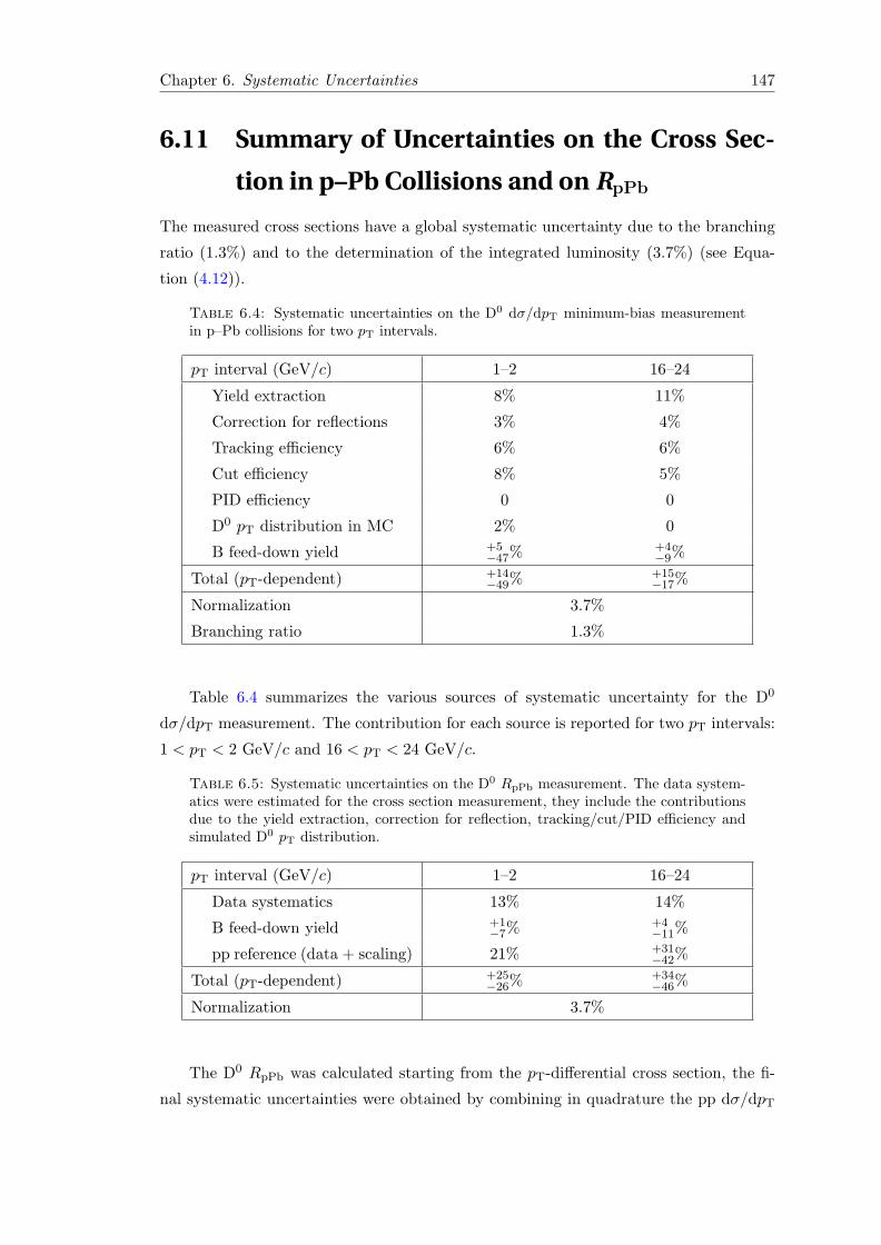
Chapter 6. Systematic Uncertainties 147
6.11 Summary of Uncertainties on the Cross Sec-
tion in p–Pb Collisions and on RpPb
The measured cross sections have a global systematic uncertainty due to the branching
ratio (1.3%) and to the determination of the integrated luminosity (3.7%) (see Equa-
tion (4.12)).
Table 6.4: Systematic uncertainties on the D0 dσ/dpT minimum-bias measurementin p–Pb collisions for two pT intervals.
pT interval (GeV/c) 1–2 16–24
Yield extraction 8% 11%
Correction for reflections 3% 4%
Tracking efficiency 6% 6%
Cut efficiency 8% 5%
PID efficiency 0 0
D0 pT distribution in MC 2% 0
B feed-down yield +5−47% +4
−9%
Total (pT-dependent) +14−49% +15
−17%
Normalization 3.7%
Branching ratio 1.3%
Table 6.4 summarizes the various sources of systematic uncertainty for the D0
dσ/dpT measurement. The contribution for each source is reported for two pT intervals:
1 < pT < 2 GeV/c and 16 < pT < 24 GeV/c.
Table 6.5: Systematic uncertainties on the D0 RpPb measurement. The data system-atics were estimated for the cross section measurement, they include the contributionsdue to the yield extraction, correction for reflection, tracking/cut/PID efficiency andsimulated D0 pT distribution.
pT interval (GeV/c) 1–2 16–24
Data systematics 13% 14%
B feed-down yield +1−7% +4
−11%
pp reference (data + scaling) 21% +31−42%
Total (pT-dependent) +25−26% +34
−46%
Normalization 3.7%
The D0 RpPb was calculated starting from the pT-differential cross section, the fi-
nal systematic uncertainties were obtained by combining in quadrature the pp dσ/dpT

Chapter 6. Systematic Uncertainties 148
and the p–Pb dσ/dpT uncertainties (Table 6.4), except for the branching ratio uncer-
tainty (which cancels in the ratio) and the feed-down correction contribution (which also
partially cancels). Table 6.5 summarizes systematic uncertainties that affect the RpPb
measurement.
The summary of the systematic uncertainties estimated for the double pT- and y-
differential cross section measurement are reported in Tables 6.6, 6.7 and 6.8.
Table 6.6: Systematic uncertainties on the D0 d2σ/dpTdy measurement in 2 < pT <5 GeV/c for the five ylab intervals considered in the analysis.
pT interval (GeV/c) 2–5
ylab interval (−0.7,−0.4) (−0.4,−0.1) (−0.1, 0.1) (0.1, 0.4) (0.4, 0.7)
Yield extraction 4% 3% 10% 3% 4%
Correction for reflections 3% 3% 3% 3% 3%
Tracking efficiency 6% 6% 6% 6% 6%
Cut efficiency 5% 5% 5% 5% 5%
PID efficiency 0 0 0 0 0
D0 pT distribution in MC 8% 8% 8% 8% 8%
B feed-down yield +4−20% +5
−22% +5−22% +5
−22% +5−21%
Total (ylab-dependent) +13−23% +13
−25% +16−27% +13
−25% +13−24%
Normalization 3.7%
Branching ratio 1.3%
Table 6.7: Systematic uncertainties on the D0 d2σ/dpTdy measurement in 5 < pT <8 GeV/c for the five ylab intervals considered in the analysis.
pT interval (GeV/c) 5–8
ylab interval (−0.8,−0.4) (−0.4,−0.1) (−0.1, 0.1) (0.1, 0.4) (0.4, 0.8)
Yield extraction 5% 5% 10% 5% 5%
Correction for reflections 3% 3% 3% 3% 3%
Tracking efficiency 6% 6% 6% 6% 6%
Cut efficiency 5% 5% 5% 5% 5%
PID efficiency 0 0 0 0 0
D0 pT distribution in MC 2% 2% 2% 2% 2%
B feed-down yield +5−12% +5
−12% +5−12% +5
−12% +5−11%
Total (ylab-dependent) +11−15% +11
−15% +14−18% +11
−15% +11−15%
Normalization 3.7%
Branching ratio 1.3%
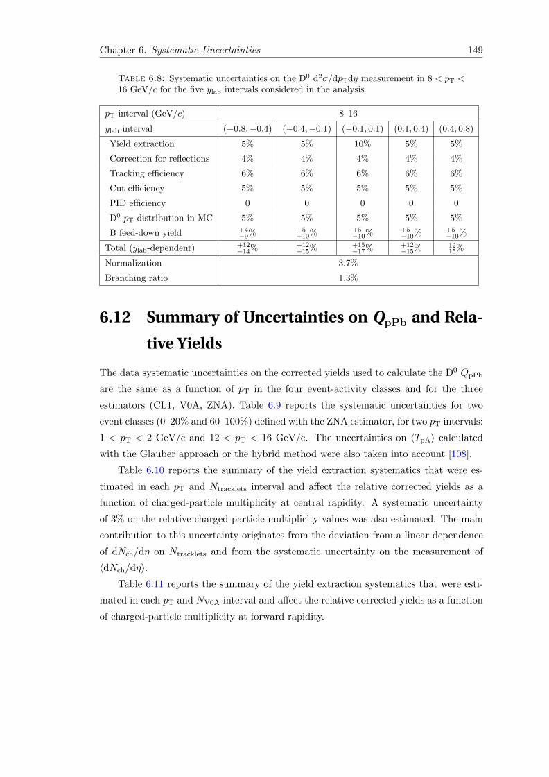
Chapter 6. Systematic Uncertainties 149
Table 6.8: Systematic uncertainties on the D0 d2σ/dpTdy measurement in 8 < pT <16 GeV/c for the five ylab intervals considered in the analysis.
pT interval (GeV/c) 8–16
ylab interval (−0.8,−0.4) (−0.4,−0.1) (−0.1, 0.1) (0.1, 0.4) (0.4, 0.8)
Yield extraction 5% 5% 10% 5% 5%
Correction for reflections 4% 4% 4% 4% 4%
Tracking efficiency 6% 6% 6% 6% 6%
Cut efficiency 5% 5% 5% 5% 5%
PID efficiency 0 0 0 0 0
D0 pT distribution in MC 5% 5% 5% 5% 5%
B feed-down yield +4−9% +5
−10% +5−10% +5
−10% +5−10%
Total (ylab-dependent) +12−14% +12
−15% +15−17% +12
−15% 1215%
Normalization 3.7%
Branching ratio 1.3%
6.12 Summary of Uncertainties on QpPb and Rela-
tive Yields
The data systematic uncertainties on the corrected yields used to calculate the D0 QpPb
are the same as a function of pT in the four event-activity classes and for the three
estimators (CL1, V0A, ZNA). Table 6.9 reports the systematic uncertainties for two
event classes (0–20% and 60–100%) defined with the ZNA estimator, for two pT intervals:
1 < pT < 2 GeV/c and 12 < pT < 16 GeV/c. The uncertainties on 〈TpA〉 calculated
with the Glauber approach or the hybrid method were also taken into account [108].
Table 6.10 reports the summary of the yield extraction systematics that were es-
timated in each pT and Ntracklets interval and affect the relative corrected yields as a
function of charged-particle multiplicity at central rapidity. A systematic uncertainty
of 3% on the relative charged-particle multiplicity values was also estimated. The main
contribution to this uncertainty originates from the deviation from a linear dependence
of dNch/dη on Ntracklets and from the systematic uncertainty on the measurement of
〈dNch/dη〉.Table 6.11 reports the summary of the yield extraction systematics that were esti-
mated in each pT and NV0A interval and affect the relative corrected yields as a function
of charged-particle multiplicity at forward rapidity.
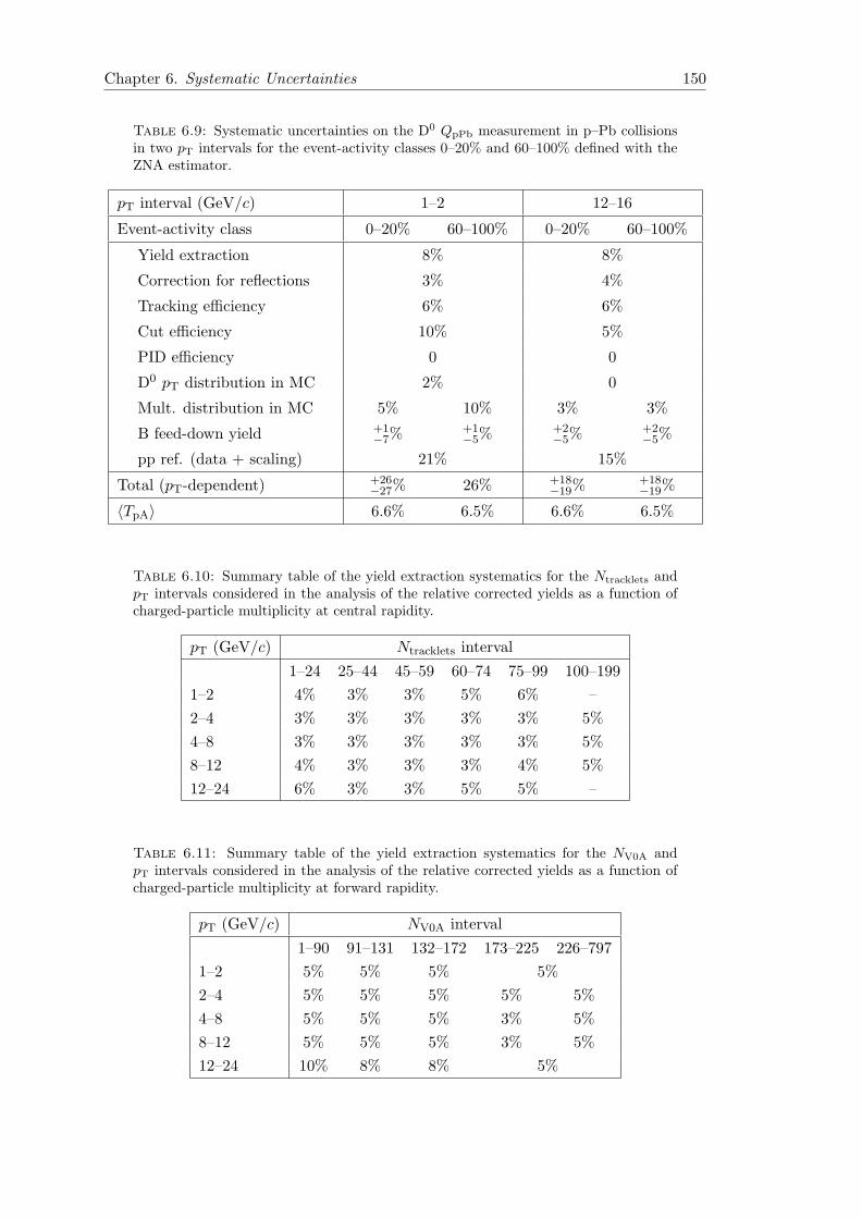
Chapter 6. Systematic Uncertainties 150
Table 6.9: Systematic uncertainties on the D0 QpPb measurement in p–Pb collisionsin two pT intervals for the event-activity classes 0–20% and 60–100% defined with theZNA estimator.
pT interval (GeV/c) 1–2 12–16
Event-activity class 0–20% 60–100% 0–20% 60–100%
Yield extraction 8% 8%
Correction for reflections 3% 4%
Tracking efficiency 6% 6%
Cut efficiency 10% 5%
PID efficiency 0 0
D0 pT distribution in MC 2% 0
Mult. distribution in MC 5% 10% 3% 3%
B feed-down yield +1−7% +1
−5% +2−5% +2
−5%
pp ref. (data + scaling) 21% 15%
Total (pT-dependent) +26−27% 26% +18
−19% +18−19%
〈TpA〉 6.6% 6.5% 6.6% 6.5%
Table 6.10: Summary table of the yield extraction systematics for the Ntracklets andpT intervals considered in the analysis of the relative corrected yields as a function ofcharged-particle multiplicity at central rapidity.
pT (GeV/c) Ntracklets interval
1–24 25–44 45–59 60–74 75–99 100–199
1–2 4% 3% 3% 5% 6% –
2–4 3% 3% 3% 3% 3% 5%
4–8 3% 3% 3% 3% 3% 5%
8–12 4% 3% 3% 3% 4% 5%
12–24 6% 3% 3% 5% 5% –
Table 6.11: Summary table of the yield extraction systematics for the NV0A andpT intervals considered in the analysis of the relative corrected yields as a function ofcharged-particle multiplicity at forward rapidity.
pT (GeV/c) NV0A interval
1–90 91–131 132–172 173–225 226–797
1–2 5% 5% 5% 5%
2–4 5% 5% 5% 5% 5%
4–8 5% 5% 5% 3% 5%
8–12 5% 5% 5% 3% 5%
12–24 10% 8% 8% 5%

7Azimuthal Anisotropy of D0 Produc-
tion in Pb–Pb Collisions
The results on the azimuthal anisotropy of D meson production in Pb–Pb collisions
at√sNN = 2.76 TeV are presented in this chapter. The azimuthal anisotropy was
quantified in terms of the elliptic flow v2 and of the nuclear modification factor RAA,
measured in the direction of the event plane and orthogonal to it. Section 7.1 is devoted
to the v2 results: the D0 elliptic flow is presented as a function of pT in the 30–50%
centrality class. v2 was also measured in the 0–10% and 10–30% centrality classes to
investigate its dependence on the collision centrality. The average D meson elliptic flow
is compared in this section with the charged-particle v2 measured with the event-plane
method. The results of the D0 RAA measured in the in-plane and in the out-of-plane
regions, in the 30–50% centrality class, are presented in Section 7.3. Section 7.4 is
devoted to the comparison of the average D meson v2 in the 30–50% centrality class,
the average D meson nuclear modification factor in 0–20% Pb–Pb collisions, and the D0
meson RAA in-plane and out-of-plane to theoretical calculations.
7.1 Elliptic Flow
The D0 elliptic flow v2 measured in Pb–Pb collisions in the 30–50% centrality class with
the event-plane method is shown as a function of pT in Figure 7.1 [67]. The v2 measure-
ment was performed also for the D+ and D∗+ mesons (Figure 7.2). The event plane was
estimated with TPC tracks in 0 < η < 0.8, as explained in Section 5.2. The symbols
are positioned horizontally at the average pT of reconstructed D mesons. This value was
determined as the average of the pT distribution of candidates in the signal invariant
mass region, after subtracting the contribution of the background candidates, which was
estimated from the side bands. The average pT of the reconstructed D mesons is larger
151

Chapter 7. Azimuthal Anisotropy of D0 Production 152
)c (GeV/T
p0 2 4 6 8 10 12 14 16 18
2v
0.3
0.2
0.1
0
0.1
0.2
0.3
0.4
0.5
0.6 0D,
0Prompt D
|y|<0.8
=2.76 TeVNN
sPbPb,
Centrality 3050%
ALICE
Figure 7.1: Elliptic flow v2 as a function of pT for prompt D0 mesons measured withthe event-plane method in Pb–Pb collisions in the 30–50% centrality class [67].
(GeV/c)T
p2 4 6 8 10 12 14 16 18
2v
0.2
0
0.2
0.4
0.6
= 2.76 TeVNNsPbPb,
Centrality 3050%
0D , 0Prompt D|y|<0.8
ALICE
(GeV/c)T
p2 4 6 8 10 12 14 16 18
0.2
0
0.2
0.4
0.6 ±Prompt D|y|<0.8
(GeV/c)T
p2 4 6 8 10 12 14 16 18
0.2
0
0.2
0.4
0.6 ±Prompt D*|y|<0.8
Open box: syst. from data
Shaded box: syst. from B feeddown
ALI−PUB−48699
Figure 7.2: v2 as a function of pT for prompt D0, D+, and D∗+ mesons for Pb–Pbcollisions in the 30–50% centrality class [67].
than that of the produced D mesons, because the efficiency increases with increasing
pT (see Figure 5.25). The vertical error bars represent the statistical uncertainty, the
open boxes are the systematic uncertainties from the anisotropy determination and the
event-plane resolution, and the filled boxes are the uncertainties due to B feed-down
contribution. The elliptic flow of the three D meson species is consistent within statisti-
cal uncertainties and ranges between 0.1 and 0.3 in the interval 2 < pT < 8 GeV/c. For
pT > 12 GeV/c, v2 is consistent with zero within the large statistical uncertainties.
For the 30–50% centrality class, an average v2 of D0, D+ and D∗+ was computed
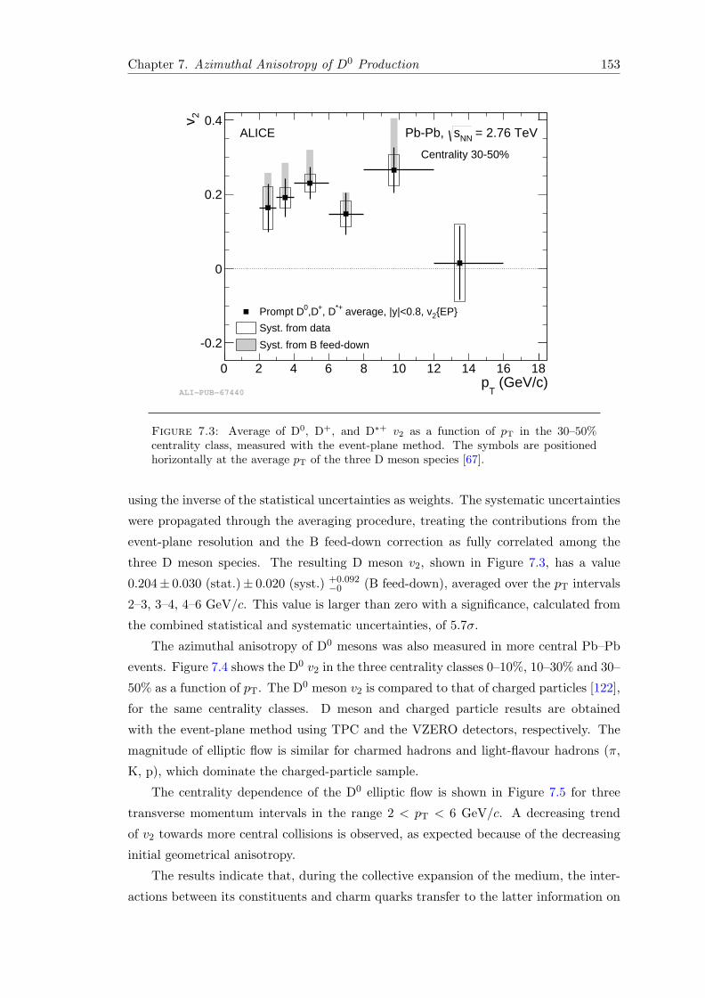
Chapter 7. Azimuthal Anisotropy of D0 Production 153
(GeV/c)T
p0 2 4 6 8 10 12 14 16 18
2v
0.2
0
0.2
0.4
{EP}2v average, |y|<0.8, *+, D+,D0Prompt D
Syst. from data
Syst. from B feeddown
= 2.76 TeVNNsPbPb,
Centrality 3050%
ALICE
ALI−PUB−67440
Figure 7.3: Average of D0, D+, and D∗+ v2 as a function of pT in the 30–50%centrality class, measured with the event-plane method. The symbols are positionedhorizontally at the average pT of the three D meson species [67].
using the inverse of the statistical uncertainties as weights. The systematic uncertainties
were propagated through the averaging procedure, treating the contributions from the
event-plane resolution and the B feed-down correction as fully correlated among the
three D meson species. The resulting D meson v2, shown in Figure 7.3, has a value
0.204± 0.030 (stat.)± 0.020 (syst.) +0.092−0 (B feed-down), averaged over the pT intervals
2–3, 3–4, 4–6 GeV/c. This value is larger than zero with a significance, calculated from
the combined statistical and systematic uncertainties, of 5.7σ.
The azimuthal anisotropy of D0 mesons was also measured in more central Pb–Pb
events. Figure 7.4 shows the D0 v2 in the three centrality classes 0–10%, 10–30% and 30–
50% as a function of pT. The D0 meson v2 is compared to that of charged particles [122],
for the same centrality classes. D meson and charged particle results are obtained
with the event-plane method using TPC and the VZERO detectors, respectively. The
magnitude of elliptic flow is similar for charmed hadrons and light-flavour hadrons (π,
K, p), which dominate the charged-particle sample.
The centrality dependence of the D0 elliptic flow is shown in Figure 7.5 for three
transverse momentum intervals in the range 2 < pT < 6 GeV/c. A decreasing trend
of v2 towards more central collisions is observed, as expected because of the decreasing
initial geometrical anisotropy.
The results indicate that, during the collective expansion of the medium, the inter-
actions between its constituents and charm quarks transfer to the latter information on

Chapter 7. Azimuthal Anisotropy of D0 Production 154
)c (GeV/T
p2 4 6 8 10 12 14 16 18
2v
0.2
0
0.2
0.4
0.6
= 2.76 TeVNNsPbPb,
Centrality 010%
ALICE
)c (GeV/T
p2 4 6 8 10 12 14 16 18
0.2
0
0.2
0.4
0.6
Centrality 1030%
{EP}2v|<0.8, y |0Prompt D
Syst. from data
Syst. from B feeddown
|>2}η∆{EP,|2vCharged particles,
)c (GeV/T
p2 4 6 8 10 12 14 16 18
0.2
0
0.2
0.4
0.6
Centrality 3050%
ALI−PUB−70100
Figure 7.4: Comparison of prompt D0 meson and charged-particle v2 [122] in threecentrality classes as a function of pT. Both measurements were done with the event-plane method [111].
Centrality (%)0 5 10 15 20 25 30 35 40 45 50
2v
0
0.05
0.1
0.15
0.2
0.25
0.3
= 2.76 TeVNNsPbPb,
ALICE
EP TPC<3 GeV/c
Tp2<
<4 GeV/cT
p3<<6 GeV/c
Tp4<
Syst. from B feeddown not shown
0D , 0Prompt D
|<0.8y|
ALI−PUB−70112
Figure 7.5: D0 meson v2 with the event-plane method in three pT intervals as afunction of centrality [111].
the azimuthal anisotropy of the system.

Chapter 7. Azimuthal Anisotropy of D0 Production 155
2 4 6 8 10 12 14 16 18
2v
0.2
0
0.2
0.4
0.6 0D ,
0Prompt D
|<0.8y|
{EP TPC}2
v
)c (GeV/T
p2 4 6 8 10 12 14 16 18
0.2
0
0.2
0.4
0.6{SP TPC}
2vALICE
= 2.76 TeVNN
sPbPb,
Centrality 3050%
2 4 6 8 10 12 14 16 18
0.2
0
0.2
0.4
0.6{2}
2v
Open box: syst. from data
Shaded box: syst. from B feeddown
Figure 7.6: D0 meson v2 as a function of pT in the 30–50% centrality class, with theevent-plane, scalar product and two-particle cumulant methods. For the first method,the event plane was estimated with TPC tracks in the positive η region; for the othermethods, TPC tracks in −0.8 < η < 0.8 were used as reference particles [111].
7.2 Comparison with Other Methods for v2 Measure-
ment
The v2 measured with the event-plane method using reference particles from the TPC
detector could be affected by non-flow correlations, because the η range of the reference
particles overlaps with the D meson acceptance. Non-flow correlations originate from
momentum conservation, quantum statistics, resonance or cascade-like decays and from
jets. The D0 v2 was also measured [111] with respect to the event plane obtained from
the VZERO detectors (i.e. with a large η-gap with respect to the D mesons), with a
scalar product [123] and a two-particle cumulant [124] methods. These methods allow
to reduce the the non-flow effects in the measured v2. The elliptic flow was computed
with the scalar product method by correlating D mesons from the positive η region
with the charged particles in the negative η region, and vice versa. This separation
in pseudorapidity suppresses two-particle correlations at short distance attributable to
decays (D∗ → D + X and B∗ → D(∗) + X). The two-particle cumulant is an average
of two-particle correlation, different order cumulants provide independent estimates for
the same harmonic coefficient vn. Orders higher than two are less affected by non-flow
effects, but the D meson analysis was doable considering two-particle correlations only,
given the available statistics.
Figure 7.6 shows the D0 v2 measured with the event-plane, scalar product and two-
particle cumulant methods. The results from the three methods are consistent within
statistical uncertainties.
Figure 7.7 shows the elliptic flow of the D0 mesons measured with the event-plane
and scalar product methods using reference particles from the TPC detector or from the
VZERO detectors (η-gap of ∆η ≥ 0.9 between D0 mesons and reference particles). The

Chapter 7. Azimuthal Anisotropy of D0 Production 156
2 4 6 8 10 12 14 16 18
2v
0.2
0
0.2
0.4
0.6 ALICE0D , 0Prompt D
|<0.8y|
(a)
EP TPC
EP VZERO
)c (GeV/T
p2 4 6 8 10 12 14 16 18
0.2
0
0.2
0.4
0.6 = 2.76 TeVNNsPbPb,
Centrality 3050%
SP TPC
SP VZERO
Syst. from B feeddown not shown
(b)
ALI−PUB−70092
Figure 7.7: D0 meson v2 as a function of pT in the 30–50% centrality class, withreference particles from TPC or from the VZERO detectors. (a) Event-plane method.(b) Scalar product method [111].
agreement between the results with and without η-gap indicates that the bias owing to
non-flow correlations is within the statistical precision of the measurement.
7.3 RAA In and Out of the Event Plane
The nuclear modification factors of D0 mesons in the 30–50% centrality class are shown
in Figure 7.8 for the in-plane and out-of-plane directions with respect to the event
plane. The error bars represent the statistical uncertainties, which are to a large extent
independent for the two azimuthal intervals, since they are dominated by the statistical
uncertainties of the Pb–Pb data. The uncorrelated (empty boxes), correlated (brackets),
and anti-correlated (shaded boxes) systematic uncertainties are shown separately (see
Table 6.3 for the type of correlation between the in-plane and the out-of-plane cases of
the various sources of uncertainty). The normalization uncertainty, shown as a box at
RAA = 1, is common to both measurements.
A large suppression is observed in both directions with respect to the event plane
for pT > 4 GeV/c. At lower transverse momentum, the suppression appears to be
reduced, especially in the in-plane direction, where RAA reaches unity at a pT of 2–
3 GeV/c. Overall, a stronger suppression in the out-of-plane direction is observed, where
the average path length of heavy quarks through the medium is larger. The ordering
Rout−of−planeAA < Rin−plane
AA is equivalent to the observation of v2 > 0, since Equation (4.6)
can be expressed also as
v2{EP} =π
4
Rin−planeAA −Rout−of−plane
AA
Rin−planeAA +Rout−of−plane
AA
. (7.1)

Chapter 7. Azimuthal Anisotropy of D0 Production 157
) c (GeV/T
p 0 2 4 6 8 10 12 14 16
AA
R
0
0.2
0.4
0.6
0.8
1
1.2
1.4
1.6
1.8
2
ALICE = 2.76 TeV
NNsPbPb,
Centrality 3050%0
D , 0
Prompt D|<0.5y|
In PlaneOut Of Plane Syst. UncertaintiesCorrelatedUncorrelatedAnticorrelatedGlobal Normalization
[ ]
ALI−PUB−70131
Figure 7.8: Nuclear modification factor RAA of D0 in the 30–50% centrality class intwo 90◦-wide azimuthal intervals centered on the in-plane and on the out-of-plane direc-tions. The correlated, uncorrelated and anti-correlated contributions to the systematicuncertainty are shown separately [111].
7.4 Comparison with Model Calculations
Several theoretical model calculations are available for the elliptic flow coefficient v2
and the nuclear modification factor RAA of heavy-flavour hadrons. Figure 7.9 shows
a comprehensive comparison of these models to measurements of the D0 RAA in-plane
and out-of-plane in the 30–50% centrality class, the average RAA of D0, D+ and D∗+ in
the 0–20% centrality class [63], and of the v2 averaged over the D meson species in the
centrality class 30–50% [67].
The models that were considered and compared to data are:
I WHDG [125–127]. It is a perturbative QCD calculation of parton energy loss,
including both radiative (DGLV [128]) and collisional processes. A realistic colli-
sion geometry based on the Glauber model [15] is used, without hydrodynamical
expansion, so that the anisotropy results only from path-length dependent en-
ergy loss. Hadronization is performed using vacuum fragmentation functions. The
medium density is constrained on the basis of the π0 RAA in central collisions at

Chapter 7. Azimuthal Anisotropy of D0 Production 158
(GeV/c)T
p0 2 4 6 8 10 12 14 16
2v
0.1
0
0.1
0.2
0.3
0.4 average*+, D+,D0ALICE D
Syst. from data
Syst. from B feeddown
WHDG rad+collPOWLANGCao, Qin, BassMC@sHQ+EPOS, Coll+Rad(LPM) TAMU elasticBAMPS UrQMD
= 2.76 TeVNNsPbPb,
Centrality 3050%
ALI−PUB−70164
(a)
)c (GeV/T
p0 2 4 6 8 10 12 14 16
AA
R
0
0.2
0.4
0.6
0.8
1
1.2
WHDG rad+collPOWLANGCao, Qin, BassMC@sHQ+EPOS, Coll+Rad(LPM)BAMPSTAMU elasticUrQMD
|<0.5y average, |*+, D+, D0ALICE D
= 2.76 TeVNNsPbPb,
Centrality 020%
ALI−PUB−70179
(b)
0 2 4 6 8 10 12 14 16
AA
R
0
0.2
0.4
0.6
0.8
1
1.2
1.4
1.6In PlaneOut Of Plane Syst. uncertaintiesCorrelatedUncorrelatedAnticorrelated Global normalization
[ ]
0D ,
0Prompt D
|<0.5y|
)c (GeV/T
p0 2 4 6 8 10 12 14 16
0
0.2
0.4
0.6
0.8
1
1.2
1.4
1.6ALICE
= 2.76 TeVNN
sPbPb,
Centrality 3050%
WHDG rad+collPOWLANGCao, Qin, BassMC@sHQ+EPOSBAMPSTAMU elasticUrQMD
ALI−PUB−70143
(c)
Figure 7.9: Model comparison for average D meson v2 in the 30–50% centralityclass [67] (a), average D meson RAA in the 0–20% centrality class [63] (b), D0 RAA
in-plane and out-of-plane in the 30–50% centrality class [111] (c). The seven modelscalculations are described in the text. The models WHDG rad+coll, POWLANG,TAMU elastic and UrQMD are shown by two lines that represent their uncertainty.
√sNN = 200 GeV and scaled to the LHC energy according to the increase of the
charged-particle multiplicity. The model describes well the D meson RAA in the
centrality interval 0–20% (slightly overestimating the suppression, as it does also
for charged particles [63]), and gives an almost pT-independent v2 ≈ 0.06, which is
smaller than the measured values in the range 2 < pT < 6 GeV/c. Consequently,
the difference between the in-plane and the out-of-plane RAA suppression is un-
derestimated: the model describes well the out-of-plane RAA and lies below the
in-plane RAA.
II MC@sHQ+EPOS, Coll+Rad(LPM) [129]. This pQCD model includes collisional
and radiative (with Landau-Pomeranchuk-Migdal correction [130]) energy loss
mechanisms for heavy quarks with running strong coupling constant. The medium
fluid dynamical expansion is based on the EPOS model [131, 132]. A component
of recombination of heavy quarks with light-flavour quarks from the QGP is also
Chapter 7. Azimuthal Anisotropy of D0 Production 159
incorporated in the model. This model yields a substantial anisotropy (v2 ≈ 0.12–
0.08 from low to high pT), which is close to that observed in data. The nuclear
modification factor is substantially overestimated below pT ≈ 5 GeV/c and cor-
rectly described at higher pT.
III TAMU elastic [133]. This is a heavy-flavour transport model based on collisional,
elastic processes only. The heavy-quark transport coefficient is calculated within
a non-perturbative T -matrix approach, where the interaction proceeds via reso-
nance formation that transfers momentum from the heavy quarks to the medium
constituents. The model includes hydrodynamical medium evolution, constrained
by light-flavour hadron spectra and elliptic flow data, and a component of recom-
bination of heavy quarks with light-flavour quarks from the QGP. Diffusion of
heavy-flavour hadrons in the hadronic phase is also included. The model provides
a good description of the observed suppression of D mesons over the entire pT
range. The maximum anisotropy, v2 of about 0.13 at 2 < pT < 4 GeV/c, is close
to that observed in the data. Towards larger pT, the model tends to underestimate
v2, as well as the difference of the in-plane and the out-of-plane RAA.
IV POWLANG [134, 135]. This transport model is based on collisional processes
treated within the framework of Langevin dynamics, within an expanding de-
confined medium described by relativistic viscous hydrodynamics. The transport
coefficients entering into the relativistic Langevin equation are evaluated by match-
ing the hard-thermal-loop calculation of soft collisions with a perturbative QCD
calculation for hard scatterings. Hadronization is implemented via vacuum frag-
mentation functions. This model overestimates the high-pT suppression, it yields
a value for v2 significantly smaller than observed in data and also underestimates
the difference between the in-plane and the out-of-plane suppression.
V BAMPS [119–121]. This partonic transport model is based on the Boltzmann ap-
proach to multi-parton scattering. Heavy quarks interact with the medium via
collisional processes computed with running strong coupling constant. Hadroniza-
tion is performed using vacuum fragmentation functions. The lack of radiative
processes is accounted for by scaling the binary cross section with a correction
factor, which is tuned to describe the heavy-flavour decay electron elliptic flow
and nuclear modification factor at RHIC. When applied to calculation for LHC
energy, this correction factor results in an underestimation of the D meson RAA
for pT > 5 GeV/c and a large azimuthal anisotropy, with v2 values up to 0.20,
similar to those observed in the data. The nuclear modification factors in-plane
and out-of-plane are well described up to 5 GeV/c, while for higher pT the in-plane
RAA is underestimated.
Chapter 7. Azimuthal Anisotropy of D0 Production 160
VI UrQMD [136, 137]. The Langevin approach for the transport of heavy quarks is in
this case implemented within the UrQMD model [138, 139]. This model includes a
realistic description of the medium evolution by combining hadronic transport and
ideal hydrodynamics. The transport of heavy quarks is calculated on the basis of
a resonance model with a decoupling temperature of 130 MeV. Hadronization via
quark coalescence is included. The calculation parameters are tuned to reproduce
the heavy-flavour measurements at RHIC (√sNN = 200 GeV) and kept unchanged
for calculations at the LHC energy. The model describes the measured D meson
v2, as well as RAA in the interval 4 < pT < 8 GeV/c, but it fails to reproduce the
significant suppression measured for RAA at a pT of 2–3 GeV/c.
VII Cao, Qin, Bass [140]. This model is also based on the Langevin approach. In
addition to quasi-elastic scatterings, radiative energy loss is incorporated by treat-
ing gluon radiation as an additional force term. The space-time evolution of the
medium is modeled using a viscous hydrodynamic simulation. The hadronization
of heavy quarks has a contribution based on the recombination mechanism. With
respect to [140], the curves shown in the figure were obtained with a more recent
parametrization for the nuclear shadowing of the parton distribution functions.
This model provides a good description of the RAA data in central collisions, but
it yields a value of v2 significantly smaller than the measured one (similar to the
WHDG and POWLANG models) and also underestimates the difference between
the in-plane and the out-of-plane suppression.
Overall, the anisotropy is qualitatively described by the models that include both charm
quark energy loss in a geometrically anisotropic medium and mechanisms that transfer
to charm quarks the elliptic flow induced during the system expansion. These mecha-
nisms include collisional processes (MC@sHQ+EPOS, Coll+Rad(LPM), BAMPS) and
resonance scattering with hadronization via recombination (TAMU elastic, UrQMD) in
a hydrodynamically expanding QGP. Models that do not include a collective expansion
of the medium or lack a contribution to the hadronization of charm quarks from recom-
bination with light quarks from the medium predict in general a smaller anisotropy than
observed in the data. The comparison for RAA and v2 shows that it is challenging to
simultaneously describe the large suppression of D mesons in central collisions and their
anisotropy in non-central collisions. In general, the models that are best in describing
RAA tend to underestimate v2 and the models that describe v2 tend to underestimate
the measured RAA at high pT.
8D0 Production in p–Pb Collisions
In this chapter the results obtained from the analysis of the D0 meson production in p–Pb
collisions at√sNN = 5.02 TeV are presented. The measured production cross sections
for prompt D0 mesons, as well as for prompt D+, D∗+ and D+s mesons are presented in
Section 8.1 as a function of pT and rapidity. The nuclear modification factor RpPb results
are given in Section 8.2. In this section the average D meson RpPb is also compared to
theoretical calculations and to the D meson RAA measured in central and semiperipheral
Pb–Pb collisions at√sNN = 2.76 TeV. The two last sections are devoted to the study
of the multiplicity dependence of the D0 production in p–Pb collisions: in Section 8.3
the QpPb as a function of event activity results are presented, and in Section 8.4 the
measured relative yields as a function of relative charged-particle multiplicity are given.
8.1 Production Cross Section
The production cross section of D0 mesons was measured in p–Pb collisions at the
centre-of-mass energy per nucleon pair of√sNN = 5.02 TeV. The same measurement was
performed also for the other D meson species, D+, D∗+, and D+s , that were reconstructed
in the rapidity interval |ylab| < 0.5 via their hadronic decay channels D+ → K−π+π+,
D∗+ → D0π+ and D+s → φπ+ → K−K+π+ [141].
Figure 8.1 shows the production cross sections as a function of transverse momen-
tum for prompt D0. The black bars indicate the statistical uncertainty while the boxes
indicate the systematic uncertainties due to the measurement of the corrected D meson
yields. The pT-independent normalization uncertainty of 3.7% is indicated separately.
The decay branching ratio uncertainty is not included in the boxes, as well. The mea-
surement was performed at midrapidity in the laboratory frame, which corresponds to
the interval −0.96 < ycms < 0.04 in the centre-of-mass frame, due to the rapidity shift
of the centre-of-mass induced by the different energies of the p and Pb beams.
161

Chapter 8. D0 Production in p–Pb Collisions 162
)c (GeV/T
p0 5 10 15 20 25
)c 1
b G
eVµ
) (
yd
Tp
/(d
σ2d
10
210
310
410
Open box: syst. unc. from Data
BR syst. unc. not shown
3.7% norm. unc. not shown±
ALICE=5.02 TeV
NNspPb,
<0.04cms
y0.96<
meson0
D
Figure 8.1: pT-differential inclusive production cross section of prompt D0 mesons inp–Pb collisions at
√sNN = 5.02 TeV [141].
cmsy
1.5 1 0.5 0 0.5
c)
1b
GeV
µdy
(T
/ dp
σ2 d
10
210
310
410
<5 GeV/cT
2<p<8 GeV/c
T5<p
<16 GeV/cT
8<p
Systematic uncert.
from Data
from B feeddown subtr.
3.4%) and BR syst. unc. not shown±Normalization (
=5.02 TeVNNspPb,
meson0D
Pbp
(MNR+EPS09)pA R×(FONLL) dyσd ×A
ALI−DER−61952
Figure 8.2: y-differential production cross section of prompt D0 mesons in p–Pbcollisions at
√sNN = 5.02 TeV. The D0 cross section is compared to a calculation based
on NLO pQCD including the nuclear modification of the PDFs as parametrized inEPS09NLO [73], indicated with its uncertainty, by the curves.
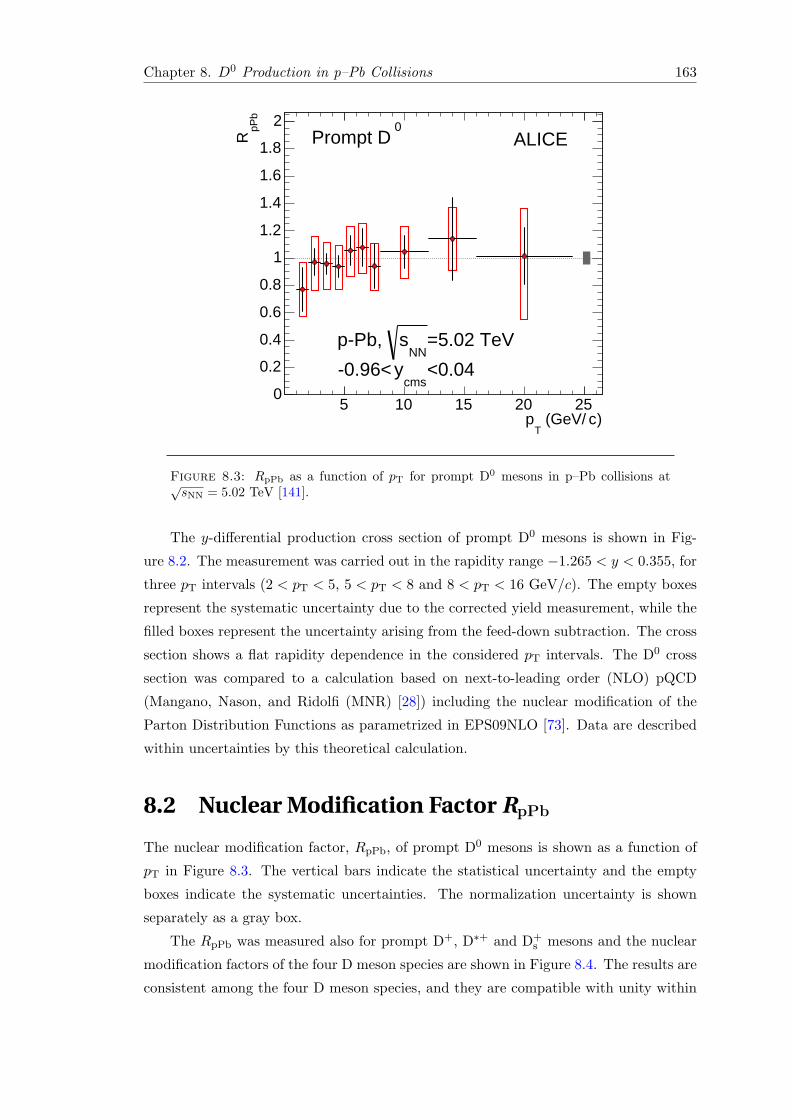
Chapter 8. D0 Production in p–Pb Collisions 163
)c (GeV/T
p5 10 15 20 25
pPb
R
0
0.2
0.4
0.6
0.8
1
1.2
1.4
1.6
1.8
2 0Prompt D
=5.02 TeVNN
spPb,
<0.04cms
y0.96<
ALICE
Figure 8.3: RpPb as a function of pT for prompt D0 mesons in p–Pb collisions at√sNN = 5.02 TeV [141].
The y-differential production cross section of prompt D0 mesons is shown in Fig-
ure 8.2. The measurement was carried out in the rapidity range −1.265 < y < 0.355, for
three pT intervals (2 < pT < 5, 5 < pT < 8 and 8 < pT < 16 GeV/c). The empty boxes
represent the systematic uncertainty due to the corrected yield measurement, while the
filled boxes represent the uncertainty arising from the feed-down subtraction. The cross
section shows a flat rapidity dependence in the considered pT intervals. The D0 cross
section was compared to a calculation based on next-to-leading order (NLO) pQCD
(Mangano, Nason, and Ridolfi (MNR) [28]) including the nuclear modification of the
Parton Distribution Functions as parametrized in EPS09NLO [73]. Data are described
within uncertainties by this theoretical calculation.
8.2 Nuclear Modification Factor RpPb
The nuclear modification factor, RpPb, of prompt D0 mesons is shown as a function of
pT in Figure 8.3. The vertical bars indicate the statistical uncertainty and the empty
boxes indicate the systematic uncertainties. The normalization uncertainty is shown
separately as a gray box.
The RpPb was measured also for prompt D+, D∗+ and D+s mesons and the nuclear
modification factors of the four D meson species are shown in Figure 8.4. The results are
consistent among the four D meson species, and they are compatible with unity within
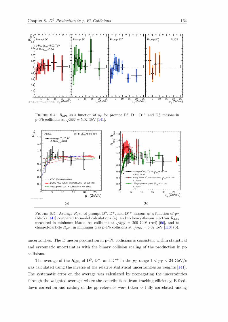
Chapter 8. D0 Production in p–Pb Collisions 164
)c (GeV/T
p5 10 15 20 25
pPb
R
0
0.2
0.4
0.6
0.8
1
1.2
1.4
1.6
1.8
20Prompt D
=5.02 TeVNNspPb, <0.04
cmsy0.96<
)c (GeV/T
p5 10 15 20 25
0
0.2
0.4
0.6
0.8
1
1.2
1.4
1.6
1.8
2+Prompt D
)c (GeV/T
p5 10 15 20 25
0
0.2
0.4
0.6
0.8
1
1.2
1.4
1.6
1.8
2+Prompt D*
)c (GeV/T
p5 10 15 20 25
0
0.2
0.4
0.6
0.8
1
1.2
1.4
1.6
1.8
2+
sPrompt D ALICE
ALI−PUB−79396
Figure 8.4: RpPb as a function of pT for prompt D0, D+, D∗+ and D+s mesons in
p–Pb collisions at√sNN = 5.02 TeV [141].
)c (GeV/T
p0 5 10 15 20 25
pPb
R
0
0.2
0.4
0.6
0.8
1
1.2
1.4
1.6 *+, D+, D0Average D<0.04
cmsy0.96<
CGC (FujiiWatanabe)
pQCD NLO (MNR) with CTEQ6M+EPS09 PDF
broad + CNM ElossT
Vitev: power corr. + k
ALICE =5.02 TeVNNspPb,
ALI−PUB−79415
(a)
)c (GeV/T
p0 5 10 15 20 25
dAu
R,
pPb
R
0
0.2
0.4
0.6
0.8
1
1.2
1.4
1.6
1.8
=5.02 TeVNN
s pPb, *+
,D+
,D0
Average D
<0.04cms
y0.96<
=200 GeVNN
s, min. bias dAu, ±
Heavy flavour e
|<0.035lab
η|
=5.02 TeVNN
sCharged particles, pPb,
|<0.03lab
η|
(b)
Figure 8.5: Average RpPb of prompt D0, D+, and D∗+ mesons as a function of pT
(black) [141] compared to model calculations (a), and to heavy-flavour electron RdAu
measured in minimum bias d–Au collisions at√sNN = 200 GeV (red) [96], and to
charged-particle RpPb in minimum bias p–Pb collisions at√sNN = 5.02 TeV [110] (b).
uncertainties. The D meson production in p–Pb collisions is consistent within statistical
and systematic uncertainties with the binary collision scaling of the production in pp
collisions.
The average of the RpPb of D0, D+, and D∗+ in the pT range 1 < pT < 24 GeV/c
was calculated using the inverse of the relative statistical uncertainties as weights [141].
The systematic error on the average was calculated by propagating the uncertainties
through the weighted average, where the contributions from tracking efficiency, B feed-
down correction and scaling of the pp reference were taken as fully correlated among

Chapter 8. D0 Production in p–Pb Collisions 165
)c (GeV/T
p0 5 10 15 20 25
Nuc
lear
mod
ifica
tion
fact
or
0
0.2
0.4
0.6
0.8
1
1.2
1.4
1.6=5.02 TeVNNspPb,
<0.04cms
y0.96<
=2.76 TeVNNsPbPb, |<0.5
cmsy|
centrality 020%centrality 4080%
ALICE*+, D+, D0Average D
ALI−PUB−79458
(a)
(GeV/c) t
p0 2 4 6 8 10 12 14 16 18
pro
mpt
DA
A R
0
0.2
0.4
0.6
0.8
1
1.2
1.4
1.6
1.8
2
ALICE020% centrality
= 2.76 TeVNNsPbPb,
NLO(MNR) with EPS09 shad.
, |y|<0.5*+, D+, D0Average D
ALI−PUB−14254
(b)
Figure 8.6: (a) Average RpPb of prompt D0, D+, and D∗+ mesons as a function ofpT [141] compared to D meson RAA in the 20% most central and in the 40–80% Pb–Pbcollisions at
√sNN = 2.76 TeV [63]. (b) Average D meson RAA in the 20% most central
Pb–Pb collisions at√sNN = 2.76 TeV compared to the expectation from NLO pQCD
with nuclear shadowing.
the three species. Figure 8.5(a) shows the average RpPb compared to theoretical calcu-
lations. Predictions based either on NLO pQCD calculations (MNR [28]) of D meson
production including EPS09NLO [73] nuclear modification of the CTEQ6M PDF [142],
or on calculations based on the Color Glass Condensate [77], can describe the mea-
surement considering only initial state effects. The results are also well described by
a calculation that includes energy loss in cold nuclear matter, nuclear shadowing, and
kT broadening [143]. The present uncertainties of the measurement do not allow any
sensitivity to a possible effect due to the formation of a hydrodynamically expanding
medium (Section 2.4), expected to be small in minimum-bias collisions at LHC energies.
Figure 8.5(b) shows the average D meson RpPb compared to the heavy-flavour electron
RdAu measured in minimum-bias d–Au collisions by PHENIX at√sNN = 200 GeV [96]
(there are no measurements of D meson RpA at RHIC yet), and to the charged-particle
RpPb measured in minimum-bias p–Pb collisions at√sNN = 5.02 TeV by ALICE [110].
The three measurements are compatible within statistical uncertainties and consistent
with unity for pT > 5 GeV/c. The charged-particle RpPb is compatible within uncer-
tainty with the D meson RpPb down to pT = 1 GeV/c, showing a less pronounced Cronin
peak with respect to the heavy-flavour electron RdAu measured at√sNN = 200 GeV.
The D meson RpPb measured at√sNN = 5.02 TeV indicates a smaller magnitude of the
Cronin effect for charm production at the LHC.
In Figure 8.6(a), the average RpPb of prompt D mesons in p–Pb collisions at√sNN =
5.02 TeV is reported along with the average prompt D meson RAA in central (0–20%)

Chapter 8. D0 Production in p–Pb Collisions 166
and in semiperipheral (40–80%) Pb–Pb collisions at√sNN = 2.76 TeV [63], showing
that cold nuclear matter effects are smaller than the uncertainties for pT & 3 GeV/c. In
addition, as reported in Ref. [63], the same EPS09 nuclear PDF parametrization that
describes the D meson RpPb results predicts small initial state effects (less than 10%
for pT > 5 GeV/c) for Pb–Pb collisions (see Figure 8.6(b)). As a consequence, the
suppression observed in central Pb–Pb collisions for pT & 2 GeV/c is predominantly
induced by final state effects, e.g. quark charm energy loss in the medium.
8.3 QpPb as a Function of Event Activity
The modification of the D0 pT distribution in p–Pb collisions with respect to the Ncoll-
scaled pp reference was measured in four event-activity classes, 0–20%, 20–40%, 40–
60%, and 60–100%, defined with three different estimators: CL1, V0A, and ZNA. The
results are shown in Figure 8.7. Figure 8.7(a) shows the D0 QpPb obtained by dividing
the visible cross section in event classes defined by the CL1 estimator, and scaling
the pp reference cross section with 〈NGlaubercoll 〉 obtained from the NBD-Glauber fit of
the multiplicity distribution of the SPD clusters (CL1). Figure 8.7(b) shows the D0
QpPb obtained by dividing the visible cross section in event classes defined by the V0A
estimator, and scaling the pp reference cross section with 〈NGlaubercoll 〉 obtained from the
NBD-Glauber fit of the distribution of the amplitudes in the VZERO-A hodoscope. The
D0 QpPb obtained with the hybrid method is shown in Figure 8.7(c). The bias on the
QpPb introduced by the determination of 〈Ncoll〉 is maximum when the CL1 estimator
is used, namely when the centrality determination was done in the same rapidity region
of the measurement, while it decreases if the forward V0A estimator is used. The least
biased measurement is obtained when defining the event-activity classes by slicing the
ZN energy deposit in the Pb-going side and applying the hybrid method to calculate
〈Ncoll〉 [108]. In this case, the modification of the D0 pT distribution with respect to pp
collisions in the four event-activity classes is consistent with unity within uncertainties,
indicating no significant event-activity dependence of the D0 production. The analysis
was performed also for the D+ and D∗+ mesons, showing consistent results [144].
8.4 Relative Yields as a Function of Multiplicity
The results on the D0 meson relative yields for each pT interval are presented in Fig-
ure 8.8 as a function of the relative charged-particle multiplicity at midrapidity (Fig-
ure 8.8(a)) and as a function of the relative uncorrected multiplicity in the VZERO-A
detector (Figure 8.8(b)). The relative yields are shown in the top panels with their
statistical (vertical bars) and systematic (boxes) uncertainties, except the uncertainty

Chapter 8. D0 Production in p–Pb Collisions 167
) c (GeV/T
p 0 5 10 15 20 25 30
pro
mpt
DC
L1pP
bQ
0
0.5
1
1.5
2
2.5
3
020%
2040%
4060%
60100%
This Thesis = 5.02 TeVNNspPb,
Filled markers : pp rescaled referenceextrapolated reference
TpOpen markers: pp
< 0.04 cms
y, 0.96 < 0Prompt D
CL1 Multiplicity
(a)
) c (GeV/T
p 0 5 10 15 20 25 30
pro
mpt
DV
0ApP
bQ
0
0.5
1
1.5
2
2.5
3
020%
2040%
4060%
60100%
This Thesis = 5.02 TeVNNspPb,
Filled markers : pp rescaled referenceextrapolated reference
TpOpen markers: pp
< 0.04 cms
y, 0.96 < 0Prompt D
V0A Multiplicity
(b)
) c (GeV/T
p 0 5 10 15 20 25 30
pro
mpt
Dm
ult
pPb
Q
0
0.5
1
1.5
2
2.5
3
020%
2040%
4060%
60100%
This Thesis = 5.02 TeVNNspPb,
Filled markers : pp rescaled referenceextrapolated reference
TpOpen markers: pp
< 0.04 cms
y, 0.96 < 0Prompt D
ZN Energy Event Classes
(c)
Figure 8.7: QpPb as a function of pT for prompt D0 measured in four event-activityclasses: 0–20% (red), 20–40% (orange), 40–60% (green), and 60–100% (blue). Theresults are shown for the three event-activity estimators considered: CL1 (a), V0A (b),and ZNA (c).
on the feed-down fraction, which is drawn separately in the bottom panels in the form
of relative uncertainties. The points are located on the x-axis at the average value of
the relative charged-particle multiplicity, (dNch/dη)/〈dNch/dη〉 for each Ntracklets inter-
val (left panel), or NV0A/〈NV0A〉 for each NV0A interval (right panel). The relative D0
yields are compatible within uncertainties in all pT intervals and they show an increasing
trend as a function of the relative charged-particle multiplicity. The relative D0 yields
increase with the charged-particle multiplicity at central rapidity by about a factor 25 in
the range between 0.5 and 4.2 times 〈dNch/dη〉, corresponding to an increase of relative
multiplicity of about a factor 9. The relative D0 yields increase by about a factor 5 in the
range between 0.5 and 3.3 times the charged-particle multiplicity at forward rapidity,
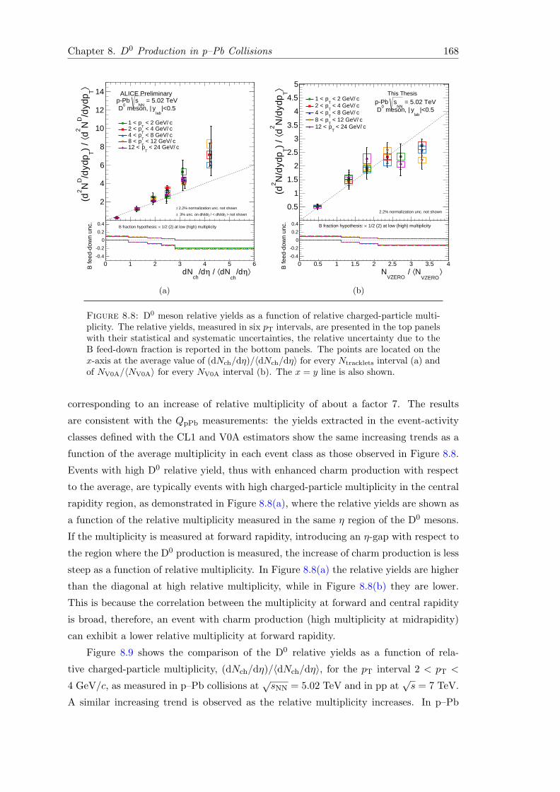
Chapter 8. D0 Production in p–Pb Collisions 168
⟩Tpdy
/dD
N2 d⟨)
/ Tpdy
/dD
N2(d 2
4
6
8
10
12
14
c < 2 GeV/T
p1 < c < 4 GeV/
Tp2 <
c < 8 GeV/T
p4 < c < 12 GeV/
Tp8 <
c < 24 GeV/T
p12 <
ALICE Preliminary = 5.02 TeV
NNspPb
|<0.5lab
y meson, |0
D
> not shownη/dN / < dη/dN 3% unc. on d±
2.2% normalization unc. not shown±
⟩η/dch
Nd⟨ / η/dch
N d0 1 2 3 4 5 6B
feed
dow
n un
c.
0.4
0.2
0
0.2
0.4 1/2 (2) at low (high) multiplicity×B fraction hypothesis:
(a)
⟩Tpdy
/dN2 d⟨
) /
Tpdy/d
N2(d
0.5
1
1.5
2
2.5
3
3.5
4
4.5
5
c < 2 GeV/T
p1 < c < 4 GeV/
Tp2 <
c < 8 GeV/T
p4 < c < 12 GeV/
Tp8 <
c < 24 GeV/T
p12 <
= 5.02 TeVNN
spPb |<0.5
laby meson, |
0D
This Thesis
2.2% normalization unc. not shown
⟩VZERO
N⟨ / VZERO
N 0 0.5 1 1.5 2 2.5 3 3.5 4B
feed
dow
n un
c.
0.4
0.2
0
0.2
0.4 1/2 (2) at low (high) multiplicity×B fraction hypothesis:
(b)
Figure 8.8: D0 meson relative yields as a function of relative charged-particle multi-plicity. The relative yields, measured in six pT intervals, are presented in the top panelswith their statistical and systematic uncertainties, the relative uncertainty due to theB feed-down fraction is reported in the bottom panels. The points are located on thex-axis at the average value of (dNch/dη)/〈dNch/dη〉 for every Ntracklets interval (a) andof NV0A/〈NV0A〉 for every NV0A interval (b). The x = y line is also shown.
corresponding to an increase of relative multiplicity of about a factor 7. The results
are consistent with the QpPb measurements: the yields extracted in the event-activity
classes defined with the CL1 and V0A estimators show the same increasing trends as a
function of the average multiplicity in each event class as those observed in Figure 8.8.
Events with high D0 relative yield, thus with enhanced charm production with respect
to the average, are typically events with high charged-particle multiplicity in the central
rapidity region, as demonstrated in Figure 8.8(a), where the relative yields are shown as
a function of the relative multiplicity measured in the same η region of the D0 mesons.
If the multiplicity is measured at forward rapidity, introducing an η-gap with respect to
the region where the D0 production is measured, the increase of charm production is less
steep as a function of relative multiplicity. In Figure 8.8(a) the relative yields are higher
than the diagonal at high relative multiplicity, while in Figure 8.8(b) they are lower.
This is because the correlation between the multiplicity at forward and central rapidity
is broad, therefore, an event with charm production (high multiplicity at midrapidity)
can exhibit a lower relative multiplicity at forward rapidity.
Figure 8.9 shows the comparison of the D0 relative yields as a function of rela-
tive charged-particle multiplicity, (dNch/dη)/〈dNch/dη〉, for the pT interval 2 < pT <
4 GeV/c, as measured in p–Pb collisions at√sNN = 5.02 TeV and in pp at
√s = 7 TeV.
A similar increasing trend is observed as the relative multiplicity increases. In p–Pb
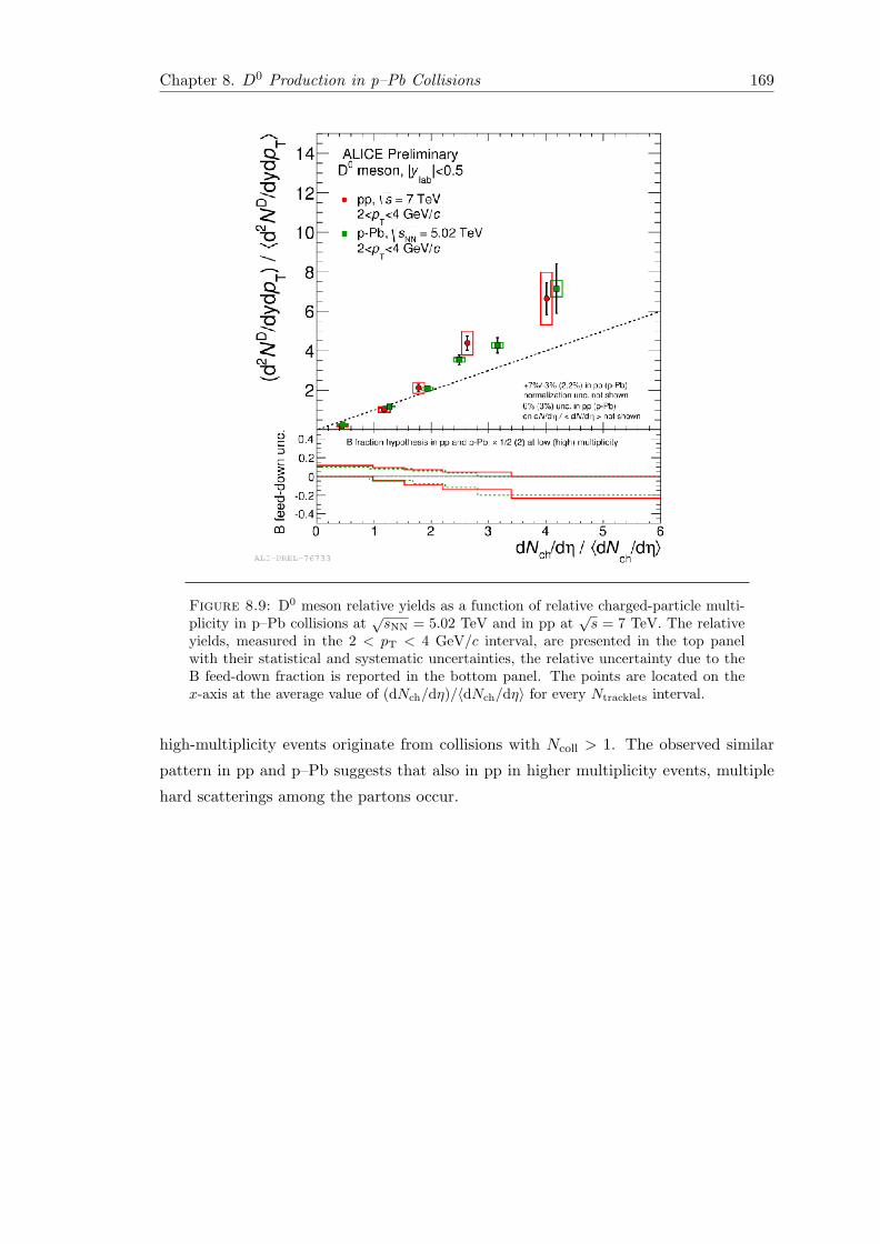
Chapter 8. D0 Production in p–Pb Collisions 169
Figure 8.9: D0 meson relative yields as a function of relative charged-particle multi-plicity in p–Pb collisions at
√sNN = 5.02 TeV and in pp at
√s = 7 TeV. The relative
yields, measured in the 2 < pT < 4 GeV/c interval, are presented in the top panelwith their statistical and systematic uncertainties, the relative uncertainty due to theB feed-down fraction is reported in the bottom panel. The points are located on thex-axis at the average value of (dNch/dη)/〈dNch/dη〉 for every Ntracklets interval.
high-multiplicity events originate from collisions with Ncoll > 1. The observed similar
pattern in pp and p–Pb suggests that also in pp in higher multiplicity events, multiple
hard scatterings among the partons occur.


Conclusions
The aims of the measurements presented in this thesis were:
– to investigate whether the charm quarks participate in the collective expansion of
the QGP,
– to assess to which extent the large suppression of the prompt D meson RAA in
central Pb–Pb collisions is a final state state effect related to the charm energy
loss in the medium.
The first question was addressed through the measurement of the azimuthal anisotropy
of the D0 meson production in semicentral Pb–Pb collisions. The second through the
measurement of the production of prompt D0 mesons in p–Pb collisions and the com-
parison to the results obtained in central Pb–Pb collisions.
The first results on the azimuthal anisotropy of D0 production at central rapid-
ity in Pb–Pb collisions at√sNN = 2.76 TeV, obtained by reconstructing the decay
D0 → K−π+, were presented. The elliptic flow coefficient v2 was measured with the
event-plane method as a function of transverse momentum for semicentral collisions in
the 30–50% quantile of the hadronic cross section. An average D meson v2 (D0, D+, and
D∗+) was calculated and in the interval 2 < pT < 6 GeV/c it is larger than zero with
a significance of 5.7σ, combining statistical and systematic uncertainties. A positive v2
is also observed for pT > 6 GeV/c, although with smaller significance, likely originating
from the path-length dependence of the in-medium partonic energy loss. The azimuthal
anisotropy of the D0 was also measured in the centrality classes 0–10% and 10–30%. For
all the three centrality classes the D0 v2 is comparable in magnitude to that of charged
particles and an indication for a decrease of elliptic flow towards more central collisions
is observed for 3 < pT < 6 GeV/c. The anisotropy was also quantified in terms of the
D0 nuclear modification factor RAA, measured in the direction of the event plane and
orthogonal to it. For pT > 3 GeV/c, a stronger suppression relative to proton–proton
collisions is observed in the out-of-plane direction, where the average path length of
heavy quarks through the medium is larger. The results for v2 and RAA azimuthal
dependence indicate that, during the collective expansion of the medium, the interac-
tions between its constituents and charm quarks transfer to the latter information on
171

Conclusions 172
the azimuthal anisotropy of the system. The measured elliptic flow and RAA in and out
of the event plane, as well as the previously published RAA in the most central Pb–Pb
collisions [63], were compared with model calculations. The anisotropy is best described
by the models that include mechanisms that transfer to charm quarks the elliptic flow
induced during the expansion. These mechanisms include collisional energy loss and
charm quark recombination with light quarks from the medium. Despite the fact that
it is challenging for models to describe simultaneously the large D meson suppression in
central collisions and their anisotropy in semiperipheral collisions, these results are cru-
cial to provide important constraints on the mechanisms of heavy-quark energy loss and
on the transport properties of the expanding medium produced in high energy Pb–Pb
collisions.
This thesis also reported the results on the measurement of the D0 cross section and
nuclear modification factor RpPb in minimum-bias p–Pb collisions at√sNN = 5.02 TeV.
The production cross section of prompt D0 mesons was measured as a function of trans-
verse momentum and rapidity. The RpPb is consistent with unity within statistical and
systematic uncertainties showing that the D0 production in p–Pb collisions is consistent
with the binary collision scaling of the production in pp collisions. The measurement is
consistent with theoretical calculations that include initial state effects such as the mod-
ification of the parton distribution functions in the nuclear environment (e.g. nuclear
shadowing and saturation of the gluon density at small parton fractional momentum),
the kT broadening induced by the multiple soft collisions of the partons before the pro-
duction of the cc pair, as well as the energy loss in cold nuclear matter.
The modification of the D0 pT distribution in p–Pb collisions with respect to the
Ncoll-scaled pp reference was also measured as a function of event activity considering
different estimators. The resultingQpPb, obtained reducing at minimum the bias induced
by Ncoll-determination, is consistent with unity within uncertainties in all event-activity
classes, indicating no significant event-activity dependence of the D0 production. The
measurement of the D0 relative yields as a function of the relative charged-particle
multiplicity is also reported. An increasing trend as a function of the relative charged-
particle multiplicity, with a milder increase at forward with respect to central rapidity is
observed. The D0 relative yields as a function of the relative charged-particle multiplicity
at midrapidity measured in p–Pb collisions were compared to those measured in pp
collisions at√s = 7 TeV, showing a similar increasing trend. In p–Pb high-multiplicity
events originate from collisions with Ncoll > 1, and the observed similar pattern in pp
and p–Pb suggests that also in higher multiplicity pp events multiple hard scatterings
among the partons occur.
The average D meson RpPb was compared to the prompt D meson nuclear modifi-
cation factor RAA measured in central and semiperipheral Pb–Pb collisions at√sNN =
2.76 TeV. This comparison shows that the cold nuclear matter effects are smaller than

Conclusions 173
the RAA uncertainties for pT & 3 GeV/c, demonstrating that the suppression observed
in central Pb–Pb collisions for pT & 2 GeV/c is predominantly induced by final state
effects, e.g. the charm energy loss in the QGP.


Bibliography
[1] T. van Ritbergen, J.A.M. Vermaseren, and S.A. Larin. The Four Loop Beta
Function in Quantum Chromodynamics. Phys. Lett. B, 400:379–384, 1997.
[2] David J. Gross and Frank Wilczek. Ultraviolet Behavior of Non-Abelian Gauge
Theories. Phys. Rev. Lett., 30:1343–1346, Jun 1973.
[3] David J. Gross and Frank Wilczek. Asymptotically Free Gauge Theories. I. Phys.
Rev. D, 8:3633–3652, Nov 1973.
[4] David J. Gross and Frank Wilczek. Asymptotically Free Gauge Theories. II. Phys.
Rev. D, 9:980–993, Feb 1974.
[5] H. David Politzer. Reliable Perturbative Results for Strong Interactions? Phys.
Rev. Lett., 30:1346–1349, Jun 1973.
[6] H. David Politzer. Asymptotic Freedom: An Approach to Strong Interactions.
Physics Reports, 14(4):129–180, 1974. ISSN 0370-1573.
[7] K.A. Olive et al. Review of Particle Physics. Chin. Phys. C, 38:090001, 2014.
[8] Kenneth G. Wilson. Confinement of Quarks. Phys. Rev. D, 10:2445–2459, Oct
1974.
[9] R. Hagedorn. Statistical Thermodynamics of Strong Interactions at High Energy.
Suppl. Nuovo Cimento, 3:147, 1965.
[10] N. Cabibbo and G. Parisi. Exponential Hadronic Spectrum and Quark Liberation.
Phys. Lett. B, 59(1):67–69, 1975.
[11] F. Karsch. Lattice QCD at High Temperature and Density. Lect. Notes Phys.,
583:209–249, 2002.
[12] Bertrand C. Barrois. Superconducting Quark Matter. Nucl. Phys. B, 129:390,
1977.
[13] Kenji Fukushima and Tetsuo Hatsuda. The Phase Diagram of Dense QCD. Reports
on Progress in Physics, 74(1):014001, 2011.
175
Bibliography 176
[14] F. Karsch and E. Laermann. Thermodynamics and In-Medium Hadron Properties
from Lattice QCD. [arXiv:hep-lat/0305025]. 2003.
[15] Michael L. Miller, Klaus Reygers, Stephen J. Sanders, and Peter Steinberg.
Glauber Modeling in High-Energy Nuclear Collisions. Ann. Rev. Nucl. Part. Sci.,
57:205–243, 2007.
[16] B. Abelev et al. Centrality Determination of Pb–Pb Collisions at√sNN = 2.76
TeV with ALICE. Phys. Rev. C, 88:044909, Oct 2013.
[17] K. Aamodt et al. Charged-Particle Multiplicity Density at Midrapidity in Central
Pb–Pb Collisions at√sNN = 2.76 TeV. Phys. Rev. Lett., 105:252301, Dec 2010.
[18] J. D. Bjorken. Highly Relativistic Nucleus–Nucleus Collisions: The Central Ra-
pidity Region. Phys. Rev. D, 27:140–151, Jan 1983.
[19] Krisztian Krajczar on behalf of the CMS Collaboration. Charged Hadron Multi-
plicity and Transverse Energy Densities in Pb–Pb Collisions from CMS. Journal
of Physics G: Nuclear and Particle Physics, 38(12):124041, 2011.
[20] Michael Annan Lisa, Scott Pratt, Ron Soltz, and Urs Wiedemann. Femtoscopy in
Relativistic Heavy-Ion Collisions. Ann. Rev. Nucl. Part. Sci., 55:357–402, 2005.
[21] K. Aamodt et al. Two-pion Bose-Einstein Correlations in Central Pb–Pb Collisions
at√sNN=2.76 TeV. Phys. Lett. B, 696:328–337, 2011.
[22] A. Adare et al. Enhanced Production of Direct Photons in Au–Au Collisions at√sNN = 200 GeV and Implications for the Initial Temperature. Phys. Rev. Lett.,
104:132301, 2010.
[23] T. Matsui and H. Satz. J/ψ Suppression by Quark-Gluon Plasma Formation.
Phys. Lett. B, 178(4):416–422, 1986.
[24] B. Abelev et al. Centrality, Rapidity and Transverse Momentum Dependence of
J/ψ Suppression in Pb–Pb Collisions at√sNN=2.76 TeV. Phys. Lett. B, 734:
314–327, 2014.
[25] S. Chatrchyan et al. Suppression of Non-Prompt J/ψ, Prompt J/ψ, and Y(1S) in
Pb–Pb Collisions at√sNN = 2.76 TeV. JHEP, 1205:063, 2012.
[26] S. et al. Chatrchyan. Observation of Sequential Υ Suppression in Pb–Pb Collisions.
Phys. Rev. Lett., 109:222301, Nov 2012.
[27] B. Abelev et al. Suppression of Υ(1S) at Forward Rapidity in Pb–Pb Collisions
at√sNN=2.76 TeV. Phys. Lett. B, 738:361–372, 2014.

Bibliography 177
[28] Michelangelo L. Mangano, Paolo Nason, and Giovanni Ridolfi. Heavy-Quark Cor-
relations in Hadron Collisions at Next-to-Leading Order. Nucl. Phys. B, 373:
295–345, 1992.
[29] B.A. Kniehl, G. Kramer, I. Schienbein, and H. Spiesberger. Hadroproduction of
D and B Mesons in a Massive VFNS. AIP Conf.Proc., 792:867–870, 2005.
[30] B.A. Kniehl, G. Kramer, I. Schienbein, and H. Spiesberger. Collinear Subtractions
in Hadroproduction of Heavy Quarks. Eur. Phys. J. C, 41:199–212, 2005.
[31] B.A. Kniehl, G. Kramer, I. Schienbein, and H. Spiesberger. Inclusive Charmed-
Meson Production at the CERN LHC. Eur. Phys. J. C, 72:2082, 2012.
[32] Stefano Frixione and Bryan R. Webber. Matching NLO QCD Computations and
Parton Shower Simulations. JHEP, 0206:029, 2002.
[33] Stefano Frixione, Paolo Nason, and Bryan R. Webber. Matching NLO QCD and
Parton Showers in Heavy-Flavor Production. JHEP, 0308:007, 2003.
[34] Matteo Cacciari, Mario Greco, and Paolo Nason. The pT Spectrum in Heavy-
Flavor Hadroproduction. JHEP, 9805:007, 1998.
[35] Matteo Cacciari, Stefano Frixione, and Paolo Nason. The pT Spectrum in Heavy-
Flavor Photoproduction. JHEP, 0103:006, 2001.
[36] Matteo Cacciari, Stefano Frixione, Nicolas Houdeau, Michelangelo L. Mangano,
Paolo Nason, et al. Theoretical Predictions for Charm and Bottom Production at
the LHC. JHEP, 1210:137, 2012.
[37] S. Alekhin, G. Altarelli, N. Amapane, J. Andersen, V. Andreev, et al. HERA and
the LHC: A Workshop on the Implications of HERA for LHC physics. Proceedings,
Part B. 2005.
[38] B. Abelev et al. Measurement of Charm Production at Central Rapidity in Proton–
Proton Collisions at√s = 7 TeV. JHEP, 2012(1):128, 2012.
[39] B. Abelev et al. Measurement of Charm Production at Central Rapidity in Proton–
Proton Collisions at√s = 2.76 TeV. JHEP, 2012(7):191, 2012.
[40] ATLAS Collaboration. Comparison of D∗ Meson Production Cross Sections
with FONLL and GM-VFNS Predictions. ATL-PHYS-PUB-2011-012, ATL-COM-
PHYS-2011-912. 2011.
[41] ATLAS Collaboration. Measurement of D∗ Meson Production Cross Sections in
pp Collisions at√s = 7 TeV with the ATLAS Detector. ATLAS-CONF-2011-017,
ATLAS-COM-CONF-2011-030. 2011.

Bibliography 178
[42] LHCb Collaboration. Prompt Charm Production in pp Collisions at√s=7 TeV.
LHCb-CONF-2010-013. Dec 2010.
[43] Pavel M. Nadolsky, Hung-Liang Lai, Qing-Hong Cao, Joey Huston, Jon Pumplin,
et al. Implications of CTEQ Global Analysis for Collider Observables. Phys. Rev.
D, 78:013004, 2008.
[44] A. Adare et al. Heavy Quark Production in pp and Energy Loss and Flow of
Heavy Quarks in Au–Au Collisions at√sNN = 200 GeV. Phys. Rev. C, 84:044905,
2011.
[45] L. Adamczyk et al. Measurements of D0 and D∗ Production in pp Collisions at√s = 200 GeV. Phys. Rev. D, 86:072013, 2012.
[46] C. Lourenco and H.K. Wohri. Heavy-Flavour Hadroproduction from Fixed-Target
to Collider Energies. Phys. Rept., 433:127–180, 2006.
[47] R.J. Fries, Berndt Muller, C. Nonaka, and S.A. Bass. Hadronization in Heavy-Ion
Collisions: Recombination and Fragmentation of Partons. Phys. Rev. Lett., 90:
202303, 2003.
[48] P. Koch, Berndt Muller, and Johann Rafelski. Strangeness in Relativistic Heavy-
Ion Collisions. Phys. Rept., 142:167–262, 1986.
[49] Inga Kuznetsova and Johann Rafelski. Heavy-Flavor Hadrons in Statistical
Hadronization of Strangeness-Rich QGP. Eur. Phys. J. C, 51:113–133, 2007.
[50] Min He, Rainer J. Fries, and Ralf Rapp. Ds-Meson as Quantitative Probe of Dif-
fusion and Hadronization in Nuclear Collisions. Phys. Rev. Lett., 110(11):112301,
2013.
[51] Stephane Peigne and Andre Peshier. Collisional Energy Loss of a Fast Heavy
Quark in a Quark-Gluon Plasma. Phys. Rev. D, 77:114017, 2008.
[52] Ralf Rapp and Hendrik van Hees. Heavy Quarks in the Quark-Gluon Plasma.
[arXiv:0903.1096]. 2009.
[53] H. van Hees, M. Mannarelli, V. Greco, and R. Rapp. Nonperturbative Heavy-
Quark Diffusion in the Quark-Gluon Plasma. Phys. Rev. Lett., 100:192301, 2008.
[54] Andre Peshier. Turning on the Charm. Nucl. Phys. A, 888:7–22, 2012.
[55] P.B. Gossiaux and J. Aichelin. Towards an Understanding of the RHIC Single
Electron Data. Phys. Rev. C, 78:014904, 2008.
Bibliography 179
[56] Steven S. Gubser. Comparing the Drag Force on Heavy Quarks in N=4 Super-
Yang-Mills Theory and QCD. Phys. Rev. D, 76:126003, 2007.
[57] R. Baier, Yuri L. Dokshitzer, Alfred H. Mueller, S. Peigne, and D. Schiff. Radiative
Energy Loss of High-Energy Quarks and Gluons in a Finite Volume Quark-Gluon
Plasma. Nucl. Phys. B, 483:291–320, 1997.
[58] R. Baier, Yuri L. Dokshitzer, Alfred H. Mueller, S. Peigne, and D. Schiff. Radiative
Energy Loss and pT-Broadening of High-Energy Partons in Nuclei. Nucl. Phys.
B, 484:265–282, 1997.
[59] Yuri L. Dokshitzer and D.E. Kharzeev. Heavy-Quark Colorimetry of QCD Matter.
Phys. Lett. B, 519:199–206, 2001.
[60] G. Aad et al. Observation of a Centrality-Dependent Dijet Asymmetry in Lead–
Lead Collisions at√sNN = 2.76 TeV with the ATLAS Detector at the LHC. Phys.
Rev. Lett., 105:252303, 2010.
[61] S. Chatrchyan et al. Observation and Studies of Jet Quenching in Pb–Pb Collisions
at Nucleon–Nucleon Center-of-Mass Energy = 2.76 TeV. Phys. Rev. C, 84:024906,
2011.
[62] L. Adamczyk et al. Observation of D0 Meson Nuclear Modifications in Au–Au
Collisions at√sNN=200 GeV. Phys. Rev. Lett., 113:142301, 2014.
[63] B. Abelev et al. Suppression of High-Transverse Momentum D Mesons in Central
Pb–Pb Collisions at√sNN = 2.76 TeV. JHEP, 1209:112, 2012.
[64] J/ψ Results from CMS in Pb–Pb Collisions, with 150µb−1 Data. Technical Report
CMS-PAS-HIN-12-014, CERN, Geneva, 2012.
[65] Magdalena Djordjevic and Marko Djordjevic. LHC Jet Suppression of Light and
Heavy-Flavor Observables. Phys. Lett. B, 734:286–289, 2014.
[66] P. Kovtun, Dan T. Son, and Andrei O. Starinets. Viscosity in Strongly-Interacting
Quantum Field Theories from Black Hole Physics. Phys. Rev. Lett., 94:111601,
2005.
[67] B. Abelev et al. D Meson Elliptic Flow in Non-Central Pb–Pb Collisions at√sNN=2.76 TeV. Phys. Rev. Lett., 111:102301, 2013.
[68] G. Aad et al. Measurement of the Azimuthal Anisotropy for Charged Particle
Production in√sNN = 2.76 TeV Lead–Lead Collisions with the ATLAS Detector.
Phys. Rev. C, 86:014907, 2012.
Bibliography 180
[69] S. Chatrchyan et al. Measurement of the Elliptic Anisotropy of Charged Particles
Produced in Pb–Pb Collisions at Nucleon–Nucleon Center-of-mass Energy = 2.76
TeV. Phys. Rev. C, 87:014902, 2013.
[70] J. Adams et al. Azimuthal Anisotropy in Au–Au Collisions at√sNN = 200 GeV.
Phys. Rev. C, 72:014904, Jul 2005.
[71] K. Aamodt et al. Higher Harmonic Anisotropic Flow Measurements of Charged
Particles in Pb–Pb Collisions at√sNN=2.76 TeV. Phys. Rev. Lett., 107:032301,
2011.
[72] M. Arneodo. Nuclear Effects in Structure Functions. Phys. Rept., 240:301–393,
1994.
[73] K.J. Eskola, H. Paukkunen, and C.A. Salgado. EPS09: A New Generation of NLO
and LO Nuclear Parton Distribution Functions. JHEP, 0904:065, 2009.
[74] M. Hirai, S. Kumano, and T.H. Nagai. Determination of Nuclear Parton Distri-
bution Functions and Their Uncertainties in Next-to-Leading Order. Phys. Rev.
C, 76:065207, 2007.
[75] D. de Florian and R. Sassot. Nuclear Parton Distributions at Next-to-Leading
Order. Phys. Rev. D, 69:074028, 2004.
[76] ALICE Collaboration. ALICE: Physics Performance Report, Volume II. Journal
of Physics G: Nuclear and Particle Physics, 32(10):1295, 2006.
[77] Hirotsugu Fujii and Kazuhiro Watanabe. Heavy-Quark Pair Production in High-
Energy pA Collisions: Open Heavy Flavors. Nucl. Phys. A, 920:78–93, 2013.
[78] P. Tribedy and R. Venugopalan. QCD Saturation at the LHC: Comparisons of
Models to pp and AA Data and Predictions for p–Pb Collisions. Phys. Lett. B,
710:125–133, 2012.
[79] Javier L. Albacete, Adrian Dumitru, Hirotsugu Fujii, and Yasushi Nara. CGC
Predictions for p–Pb Collisions at the LHC. Nucl. Phys. A, 897:1–27, 2013.
[80] Amir H. Rezaeian. CGC Predictions for p–A Collisions at the LHC and Signature
of QCD Saturation. Phys. Lett. B, 718:1058–1069, 2013.
[81] J.W. Cronin, Henry J. Frisch, M.J. Shochet, J.P. Boymond, R. Mermod, et al.
Production of Hadrons with Large Transverse Momentum at 200 GeV, 300 GeV,
and 400 GeV. Phys. Rev. D, 11:3105, 1975.
[82] B.Z. Kopeliovich, J. Nemchik, A. Schafer, and A.V. Tarasov. Cronin Effect in
Hadron Production Off Nuclei. Phys. Rev. Lett., 88:232303, 2002.

Bibliography 181
[83] Xin-Nian Wang. Systematic Study of High-pT Hadron Spectra in pp, pA and AA
Collisions from SPS to RHIC Energies. Phys. Rev. C, 61:064910, 2000.
[84] M. Lev and B. Petersson. Nuclear Effects at Large Transverse Momentum in a
QCD Parton Model. Z. Phys. C, 21:155, 1983.
[85] I. Vitev. Non-Abelian Energy Loss in Cold Nuclear Matter. Phys. Rev. C, 75:
064906, 2007.
[86] S. Chatrchyan et al. Observation of Long-Range Near-Side Angular Correlations
in Proton–Lead Collisions at the LHC. Phys. Lett. B, 718:795–814, 2013.
[87] B. Abelev et al. Long-Range Angular Correlations on the Near and Away Side in
p–Pb Collisions at√sNN = 5.02 TeV. Phys. Lett. B, 719:29–41, 2013.
[88] B. Abelev et al. Long-Range Angular Correlations of π, K and p in p–Pb Collisions
at√sNN=5.02 TeV. Phys. Lett. B, 726:164–177, 2013.
[89] G. Aad et al. Observation of Associated Near-Side and Away-Side Long-Range
Correlations in√sNN = 5.02 TeV Proton-Lead Collisions with the ATLAS Detec-
tor. Phys. Rev. Lett., 110(18):182302, 2013.
[90] S.S. Adler et al. Nuclear Effects on Hadron Production in d–Au and pp Collisions
at√sNN=200 GeV. Phys. Rev. C, 74:024904, 2006.
[91] A. Adare et al. Nuclear Modification of ψ‘, χc, and J/ψ Production in d–Au
Collisions at√sNN=200 GeV. Phys. Rev. Lett., 111(20):202301, 2013.
[92] B. Abelev et al. Suppression of ψ(2S) Production in p-Pb Collisions at√sNN =
5.02 TeV. JHEP, 1412:073, 2014.
[93] Anne M. Sickles. Possible Evidence for Radial Flow of Heavy Mesons in d–Au
Collisions. Phys. Lett. B, 731:51–56, 2014.
[94] B. Abelev et al. Systematic Measurements of Identified Particle Spectra in pp,
d–Au and Au–Au Collisions from STAR. Phys. Rev. C, 79:034909, 2009.
[95] B. Abelev et al. Multiplicity Dependence of Pion, Kaon, Proton and Lambda
Production in p–Pb Collisions at√sNN=5.02 TeV. Phys. Lett. B, 728:25–38,
2014.
[96] A. Adare et al. Cold-Nuclear-Matter Effects on Heavy-Quark Production in d–Au
Collisions at√sNN = 200 GeV. Phys. Rev. Lett., 109(24):242301, 2012.
[97] G. Aad et al. Observation of a New Particle in the Search for the Standard Model
Higgs Boson with the ATLAS Detector at the LHC. Phys. Lett. B, 716:1–29, 2012.
Bibliography 182
[98] S. Chatrchyan et al. Observation of a New Boson at a Mass of 125 GeV with the
CMS Experiment at the LHC. Phys. Lett. B, 716:30–61, 2012.
[99] Lyndon Evans and Philip Bryant. LHC Machine. Journal of Instrumentation, 3
(08):S08001, 2008.
[100] LHC Physics Centre at CERN. http://lpcc.web.cern.ch/LPCC/.
[101] Aamodt, K. and The ALICE Collaboration. The ALICE Experiment at the CERN
LHC. Journal of Instrumentation, 3(08):S08002, 2008.
[102] R. Fruhwirth. Application of Kalman Filtering to Track and Vertex Fitting. Nu-
clear Instruments and Methods in Physics Research Section A: Accelerators, Spec-
trometers, Detectors and Associated Equipment, 262(2–3):444–450, 1987.
[103] B. Abelev et al. Performance of the ALICE Experiment at the CERN LHC. Int.
J. Mod. Phys. A, 29:1430044, 2014.
[104] Sergei A. Voloshin, Arthur M. Poskanzer, and Raimond Snellings. Collective Phe-
nomena in Non-Central Nuclear Collisions. [arXiv:0809.2949]. 2008.
[105] K. Aamodt et al. Harmonic Decomposition of Two-Particle Angular Correlations
in Pb–Pb Collisions at√sNN = 2.76 TeV. Phys. Lett. B, 708:249–264, 2012.
[106] David G. d’Enterria. Hard Scattering Cross-Sections at LHC in the Glauber Ap-
proach: From pp to pA and AA Collisions. [arXiv:nucl-ex/0302016]. 2003.
[107] B. Abelev et al. Measurement of Visible Cross Sections in Proton–Lead Collisions
at√sNN=5.02 TeV in van der Meer Scans with the ALICE Detector. JINST, 9
(11):P11003, 2014.
[108] J. Adam et al. Centrality Dependence of Particle Production in p–Pb Collisions
at√sNN= 5.02 TeV. [arXiv:1412.6828]. 2014.
[109] B. Abelev et al. Pseudorapidity Density of Charged Particles in p–Pb Collisions
at√sNN = 5.02 TeV. Phys. Rev. Lett., 110:032301, Jan 2013.
[110] B. Abelev et al. Transverse Momentum Distribution and Nuclear Modification
Factor of Charged Particles in p–Pb Collisions at√sNN = 5.02 TeV. Phys. Rev.
Lett., 110:082302, 2013.
[111] B. Abelev et al. Azimuthal Anisotropy of D Meson Production in Pb–Pb Collisions
at√sNN = 2.76 TeV. Phys. Rev. C, 90:034904, 2014.
[112] A. Dainese. Charm Production and In-Medium QCD Energy Loss in Nucleus–
Nucleus Collisions with ALICE: A Performance Study. [arXiv:nucl-ex/0311004].
2003.

Bibliography 183
[113] F. James and M. Winkler. Minuit User’s Guide. http://seal.web.cern.ch/
seal/documents/minuit/mnusersguide.pdf.
[114] Rene Brun, Federico Carminati, and Simone Giani. GEANT Detector Description
and Simulation Tool. CERN-W5013, CERN-W-5013. 1994.
[115] Xin-Nian Wang and Miklos Gyulassy. HIJING: A Monte Carlo Model for Multiple
Jet Production in pp, pA and AA Collisions. Phys. Rev. D, 44:3501–3516, 1991.
[116] Torbjorn Sjostrand, Stephen Mrenna, and Peter Z. Skands. PYTHIA 6.4 Physics
and Manual. JHEP, 0605:026, 2006.
[117] Peter Zeiler Skands. Tuning Monte Carlo Generators: The Perugia Tunes. Phys.
Rev. D, 82:074018, 2010.
[118] D.J. Lange. The EvtGen Particle Decay Simulation Package. Nucl. Instrum. Meth.
A, 462:152–155, 2001.
[119] O. Fochler, J. Uphoff, Z. Xu, and C. Greiner. Jet Quenching and Elliptic Flow at
RHIC and LHC within a pQCD-Based Partonic Transport Model. J. Phys. G, 38:
124152, 2011.
[120] Jan Uphoff, Oliver Fochler, Zhe Xu, and Carsten Greiner. Elliptic Flow and Energy
Loss of Heavy Quarks in Ultra-Relativistic Heavy-Ion Collisions. Phys. Rev. C,
84:024908, 2011.
[121] Jan Uphoff, Oliver Fochler, Zhe Xu, and Carsten Greiner. Open Heavy Flavor in
Pb–Pb Collisions at√sNN = 2.76 TeV within a Transport Model. Phys. Lett. B,
717:430–435, 2012.
[122] B. Abelev et al. Anisotropic Flow of Charged Hadrons, Pions and (Anti-)Protons
Measured at High Transverse Momentum in Pb–Pb Collisions at√sNN=2.76 TeV.
Phys. Lett. B, 719:18–28, 2013.
[123] C. Adler et al. Elliptic flow from two and four particle correlations in Au+Au
collisions at√sNN = 130 GeV. Phys. Rev. C, 66:034904, 2002.
[124] Ante Bilandzic, Raimond Snellings, and Sergei Voloshin. Flow Analysis with Cu-
mulants: Direct Calculations. Phys. Rev. C, 83:044913, 2011.
[125] Simon Wicks, William Horowitz, Magdalena Djordjevic, and Miklos Gyulassy.
Elastic, Inelastic, and Path Length Fluctuations in Jet Tomography. Nucl. Phys.
A, 784:426–442, 2007.
[126] W.A. Horowitz and Miklos Gyulassy. The Surprising Transparency of the sQGP
at LHC. Nucl. Phys. A, 872:265–285, 2011.

Bibliography 184
[127] W.A. Horowitz. Testing pQCD and AdS/CFT Energy Loss at RHIC and LHC.
AIP Conf. Proc., 1441:889–891, 2012.
[128] Magdalena Djordjevic and Miklos Gyulassy. Heavy-Quark Radiative Energy Loss
in QCD Matter. Nucl. Phys. A, 733:265–298, 2004.
[129] Marlene Nahrgang, Joerg Aichelin, Pol Bernard Gossiaux, and Klaus Werner.
Influence of Hadronic Bound States Above Tc on Heavy-Quark Observables in Pb–
Pb collisions at the CERN Large Hadron Collider. Phys. Rev. C, 89(1):014905,
2014.
[130] R. Baier, D. Schiff, and B.G. Zakharov. Energy Loss in Perturbative QCD. Ann.
Rev. Nucl. Part. Sci., 50:37–69, 2000.
[131] K. Werner, Iu. Karpenko, T. Pierog, M. Bleicher, and K. Mikhailov. Event-by-
Event Simulation of the Three-Dimensional Hydrodynamic Evolution from Flux
Tube Initial Conditions in Ultra-Relativistic Heavy-Ion Collisions. Phys. Rev. C,
82:044904, 2010.
[132] K. Werner, Iu. Karpenko, M. Bleicher, T. Pierog, and S. Porteboeuf-Houssais.
Jets, Bulk Matter, and their Interaction in Heavy-Ion Collisions at Several TeV.
Phys. Rev. C, 85:064907, 2012.
[133] Min He, Rainer J. Fries, and Ralf Rapp. Heavy Flavor at the Large Hadron
Collider in a Strong Coupling Approach. Phys. Lett. B, 735:445–450, 2014.
[134] W.M. Alberico, A. Beraudo, A. De Pace, A. Molinari, M. Monteno, et al. Heavy-
Flavour Spectra in High Energy Nucleus–Nucleus Collisions. Eur. Phys. J. C, 71:
1666, 2011.
[135] M. Monteno, W.M. Alberico, A. Beraudo, A. De Pace, A. Molinari, et al. Heavy-
Flavor Dynamics in Nucleus–Nucleus Collisions: from RHIC to LHC. J. Phys. G,
38:124144, 2011.
[136] Thomas Lang, Hendrik van Hees, Jan Steinheimer, and Marcus Bleicher. Heavy-
Quark Transport in Heavy-Ion Collisions at RHIC and LHC within the UrQMD
Transport Model. [arXiv:1211.6912]. 2012.
[137] Thomas Lang, Hendrik van Hees, Jan Steinheimer, Yu-Peng Yan, and Marcus
Bleicher. Heavy-Quark Transport at RHIC and LHC. J.Phys.Conf.Ser., 426:
012032, 2013.
[138] S.A. Bass, M. Belkacem, M. Bleicher, M. Brandstetter, L. Bravina, et al. Micro-
scopic Models for Ultra-Relativistic Heavy-Ion Collisions. Prog. Part. Nucl. Phys.,
41:255–369, 1998.

Bibliography 185
[139] M. Bleicher, E. Zabrodin, C. Spieles, S.A. Bass, C. Ernst, et al. Relativistic
Hadron–Hadron Collisions in the Ultra-Relativistic Quantum Molecular Dynamics
Model. J. Phys. G, 25:1859–1896, 1999.
[140] Shanshan Cao, Guang-You Qin, and Steffen A. Bass. Heavy-Quark Dynamics
and Hadronization in Ultra-Relativistic Heavy-Ion Collisions: Collisional Versus
Radiative Energy Loss. Phys. Rev. C, 88(4):044907, 2013.
[141] B. Abelev et al. Measurement of Prompt D-Meson Production in p–Pb Collisions
at√sNN = 5.02 TeV. Phys. Rev. Lett., 113:232301, Dec 2014.
[142] Daniel Stump, Joey Huston, Jon Pumplin, Wu-Ki Tung, H.L. Lai, et al. Inclusive
Jet Production, Parton Distributions, and the Search for New Physics. JHEP,
0310:046, 2003.
[143] Rishi Sharma, Ivan Vitev, and Ben-Wei Zhang. Light-Cone Wave Function Ap-
proach to Open Heavy Flavor Dynamics in QCD Matter. Phys. Rev. C, 80:054902,
2009.
[144] R. Russo. Measurement of Heavy-Flavour Production as a Function of Multiplicity
in pp and p–Pb Collisions with ALICE. Nucl. Phys. A, 931:552–557, 2014.

Acknowledgements
I would like to thank my supervisor, Andrea Dainese, for his constant support during my
PhD and for being always available for discussion in case of any questions or doubts I had
in these three years, his suggestions were fundamental to improve this write up. I am also
very grateful to Rosario Turrisi for his experience and the stimulating discussions I had
with him, and to all the ALICE group in Padova, that gave me the possibility to attend
schools and conferences and allowed me to spend an amazing and fruitful year at CERN.
It was a pleasure to work with Davide on the analysis and I am very grateful to him for
his help and suggestions and for the time spent learning and discussing about physics,
he became also a good friend. Thanks also to Zaida, Francesco and Ralf, they have been
great coordinators and I learnt a lot about heavy-flavour physics from the discussions
with them during the meetings of the working group. I thank Andrea, Riccardo, Cristina
and Grazia, it was a pleasure to cooperate with them in the D meson analysis.
I am very thankful to my parents for their love and for allowing me to pursue my
studies and researches, to my sister for being always with me, and to my grandparents
for being always proud of my work even if so far from their experiences.
Last, I wish to thank my dear friends Andrea, Luca, Emanuela, Carlo, Emil and
Federica, they accompanied me during these years and we shared many enjoying and
relaxing moments.
187
%d0%9d%d0%b0%d0%b2%d1%87%d0%b0%d0%bb%d1%8c%d0%bd%d0%be %d0%bc%d0%b5%d1%82%d0%be%d0%b4%d0%b8%d1%87%d0
1060204 %d0%bb%d0%b8%d1%81%d1%82%d0%be%d0%b2%d0%ba%d0%b0 %d0%bf%d0%be %d1%82%d0%b5%d0%bf%d0%bb%d0%be