measurement of two-phase flow structure in a narrow...

3

Measurement of Two-Phase Flow Structure in a Narrow Rectangular Channel

Daisuke Ito and Horst-Michael Prasser ETH Zurich Switzerland

1. Introduction

The flow channel of the fluids in the nuclear reactor core and the heat exchanger is relatively small. In order to understand the two-phase flow phenomena in the narrow channel, many interesting studies have been carried out, for example, mini capillaries (Wong, et al., 1995, Han & Shikazono, 2009), rectangular channels with small gap (Mishima, et al., 1993, Xu, et al., 1999, Hibiki & Mishima, 2001) and rod bundles with tight-lattice geometry (Tamai et al., 2006, Sadatomi et al., 2007, Kawahara et al., 2008). Especially, a triangle tight-lattice rod bundle has been adopted as a fuel rod configuration in high conversion boiling water reactor (Iwamura et al., 2006, Uchikawa et al., 2007, Fukaya et al., 2009). This has a narrow gap of about 1mm in the coolant channel. Therefore, two-phase flow in the tight-lattice bundle or narrow channel should be clarified for thermal-hydraulic analysis of high conversion reactor. In the past several years, the acquisition of experimental data and the modelling of the flow in tight-lattice rod bundle have been done. Tamai et al. (2006) evaluated the effect of the gap width and the power profile from the pressure drop measured in tight-lattice 37 rod bundles. Sadatomi et al. (2007) studied the void fraction characteristics in double subchannels with tight-lattice array and the data was compared with some correlations and subchannel codes. Furthermore, their group estimated the wall and the interfacial friction forces from the measured void fraction and pressure drop using the same subchannel (Kawahara et al., 2008). However, the advanced measurement techniques of the spatio-temporal phase distribution and velocity field are required for the high accurate analysis of the flow.

For the void fraction distribution measurement, the radiation methods have been developed to evaluate the flow in the bundle. Kureta (2007a, 2007b) developed a neutron radiography method for three-dimensional tomographic imaging of two-phase flow. The three-dimensional flow structures in the tight-lattice rod bundle were visualized. Although the spatial void fraction distribution can be obtained by the neutron imaging method, it is difficult to measure the time variation with high temporal resolution. In addition, there are some limitations of the uses. Thus, the authors focused on two-phase flow measurement using electrical conductance. Wire-mesh sensor (WMS), which uses the difference of electrical conductance between gas and liquid phases, has received attention as cross-sectional void fraction distribution measurement method (Prasser et al., 1998). To apply the WMS measurements to the flow in the rod bundle, a lot of electrode wires have to be

www.intechopen.com

Flow Measurement

74

installed over the small cross section and there are several intrusive effects to the flow (Ito et al., 2011a). Therefore, a novel void fraction measurement method with the electrodes on the wall of the flow channel was developed for two-phase flow in the narrow channel (Ito et al. 2010b). The wire electrodes were fixed on the opposing walls of the narrow channel and the conductance in the narrow gap was measured. As a result, three-dimensional void fraction distributions can be obtained. On the other hand, a liquid film sensor based on the electrical conductance measurements was developed (Damsohn & Prasser, 2009). This can estimate the liquid film thickness distribution on the wall in a flow channel. In addition, this sensor was applied to the annular flow measurement in the double subchannels of a square-lattice bundle. The liquid film behavior in the rod bundle was well visualized (Damsohn & Prasser, 2010). Thus, the novel measurement method for two-phase flow in the narrow channel has been developed by combining the void fraction detection and liquid film sensor (Ito et al., 2011c). The instantaneous distributions of the liquid film thickness on a wall and the void fraction in the gap were measured simultaneously by this method.

In this chapter, the measurement principle of the novel technique is described, and the measurements in a narrow rectangular channel with a gap width of 1.5mm are carried out by using two liquid film sensors. The liquid film thicknesses on two channel walls and the void fraction in the gap are estimated from the measured electrical conductance. In addition, the void fraction is recalculated by considering the film thickness and interfacial area concentration is obtained by reconstructing the gas-liquid interfacial structure. Furthermore, the individual bubble parameters are obtained by time-revolved reconstruction of the flow.

2. Measurement method

2.1 Principles

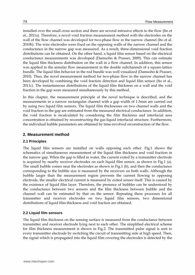
The liquid film sensors are installed on walls opposing each other. Fig.1 shows the schematics of simultaneous measurement of the liquid film thickness and void fraction in the narrow gap. When the gap is filled in water, the current exited by a transmitter electrode is acquired by nearby receiver electrodes on each liquid film sensor, as shown in Fig.1 (a). The small bubble comes near the electrodes as shown in Fig.1 (b), and then the conductance corresponding to the bubble size is measured by the receivers on both walls. Although the bubble larger than the measurement region prevents the current flowing to opposing electrode, the smaller electrical current is measured by exited sensor itself. This is caused by the existence of liquid film layer. Therefore, the presence of bubbles can be understood by the conductance between two sensors and the film thickness between bubble and the channel wall can be estimated by that on the sensor. Repeating these processes for all transmitter and receiver electrodes on two liquid film sensors, two dimensional distributions of liquid film thickness and void fraction are obtained.

2.2 Liquid film sensors

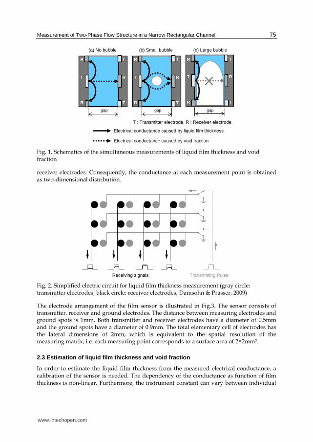
The liquid film thickness on the sensing surface is measured from the conductance between transmitter and receiver electrode lying next to each other. The simplified electrical scheme for film thickness measurement is shown in Fig.2. The transmitted pulse signal is sent to every transmitter electrode by switching the circuit of transmitting side at high speed. Then, the signal which is propagated into the liquid film covering the electrodes is detected by the

www.intechopen.com


75

T R

R T

R T

T : Transmitter electrode, R : Receiver electrode

Electrical conductance caused by void fraction

Electrical conductance caused by liquid film thickness

gap

T R

R T

R T

(a) No bubble (c) Large bubble

gapgap

T R

R T

R T

(b) Small bubble

Fig. 1. Schematics of the simultaneous measurements of liquid film thickness and void fraction

receiver electrodes. Consequently, the conductance at each measurement point is obtained as two-dimensional distribution.

Receiving signals Transmitting Pulse

Fig. 2. Simplified electric circuit for liquid film thickness measurement (gray circle: transmitter electrodes, black circle: receiver electrodes, Damsohn & Prasser, 2009)

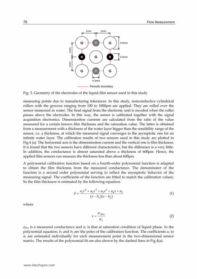
The electrode arrangement of the film sensor is illustrated in Fig.3. The sensor consists of transmitter, receiver and ground electrodes. The distance between measuring electrodes and ground spots is 1mm. Both transmitter and receiver electrodes have a diameter of 0.5mm and the ground spots have a diameter of 0.9mm. The total elementary cell of electrodes has the lateral dimensions of 2mm, which is equivalent to the spatial resolution of the measuring matrix, i.e. each measuring point corresponds to a surface area of 2×2mm2.

2.3 Estimation of liquid film thickness and void fraction

In order to estimate the liquid film thickness from the measured electrical conductance, a calibration of the sensor is needed. The dependency of the conductance as function of film thickness is non-linear. Furthermore, the instrument constant can vary between individual

www.intechopen.com

Flow Measurement

76

G

T

T

RR

G G

GG

Periodic boundary

1mm

1mm

1mm 1mm

0.5mm

0.5mm

0.9mm

Fig. 3. Geometry of the electrodes of the liquid film sensor used in this study

measuring points due to manufacturing tolerances. In this study, nonconductive cylindrical rollers with the grooves ranging from 100 to 1000μm are applied. They are rolled over the sensor immersed in water. The final signal from the electronic unit is recoded when the roller passes above the electrodes. In this way, the sensor is calibrated together with the signal acquisition electronics. Dimensionless currents are calculated from the ratio of the value measured for a certain known film thickness and the saturation value. The latter is obtained from a measurement with a thickness of the water layer bigger than the sensibility range of the sensor, i.e. a thickness, at which the measured signal converges to the asymptotic one for an infinite water layer. The calibration results of two sensors used in this study are plotted in Fig.4 (a). The horizontal axis is the dimensionless current and the vertical one is film thickness. It is found that the two sensors have different characteristics, but the difference is a very little. In addition, the conductance is almost saturated above a thickness of 600μm. Hence, the applied film sensors can measure the thickness less than about 600μm.

A polynomial calibration function based on a fourth-order polynomial function is adapted to obtain the film thickness from the measured conductance. The denominator of the function is a second order polynomial serving to reflect the asymptotic behavior of the measuring signal. The coefficients of the function are fitted to match the calibration values. So the film thickness is estimated by the following equation.

4 3 2

1 2 3 4 5

1 2( )( )

a x a x a x a x a

x b x b (1)

where

film

L

x (2)

┫film is a measured conductance and ┫L is that at saturation condition of liquid phase. In the polynomial equation, b1 and b2 are the poles of the calibration function. The coefficients a1 to a5 are estimated individually for each measurement point in the two-dimensional sensor matrix. The results of the polynomial fit are also shown by the dashed lines in Fig.4(a).

www.intechopen.com


77

0 0.2 0.4 0.6 0.8 10

100

200

300

400

500

600

700

800

Dimensionless current [-]

Film

th

ickn

ess

[m]

LFS 1 LFS2 Polynomial

0 0.5 1 1.5 2 2.5

0

0.2

0.4

0.6

0.8

1

Gap distance [mm]

Rat

io o

f sa

tura

tio

n c

urr

ent

[-]

(a) Liquid film thickness estimation (b) Saturation current between two sensors

Fig. 4. Calibration results

In the measurement, the conductance at saturation condition is measured with another sensor because the sensors are fixed in the flow channel. Since the electrodes of the opposing sensor are connected to ground potential when the film conductance is detected, the saturation conductance is influenced by the distance between two sensors. In case of the narrow gap, the conductance with another sensor becomes much smaller than that without it. Therefore, the effect of the gap distance to the conductance is measured and plotted in Fig.4 (b). The horizontal axis is the distance between two sensors and the vertical axis is a ratio of the saturation conductance between with and without the opposing sensor. It is clear that the saturation conductance depends on the distance between the sensors and greatly decreases when the gap becomes narrower. In the gap of 1.5mm, the decreasing ratio of the conductance is about 67%. Thus, in the film thickness estimation, this ratio is multiplied to the saturation conductance ┫L in Eq. (2).

In the estimation of the void fraction, the linear approximation between the void fraction and the measured conductance is applied, and so the void fraction is calculated by the following equation.

1gap

L

(3)

where ┫gap is a measured conductance between two sensors and ┫L is a saturation conductance when the flow channel is completely filled by liquid phase (water). In previous studies with WMS and μWMS, they used also the same expression to estimate the void fraction, and they obtained accurate results.

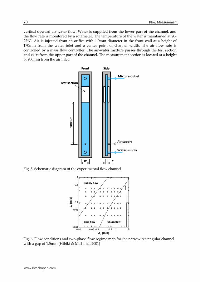
3. Experimental setup

The scheme of the test channel is given in Fig.5. The rectangular narrow channel is constructed by flanging distance plates with the desired thickness between the opposing channel walls. The length of the test channel is 1,450mm and the width is constant over height. In this study, the gap s=1.5mm and the channel width w=32mm. The flow is a

www.intechopen.com

Flow Measurement

78

vertical upward air-water flow. Water is supplied from the lower part of the channel, and the flow rate is monitored by a rotameter. The temperature of the water is maintained at 20-22°C. Air is injected from an orifice with 1.0mm diameter in the front wall at a height of 170mm from the water inlet and a center point of channel width. The air flow rate is controlled by a mass flow controller. The air-water mixture passes through the test section and exits from the upper part of the channel. The measurement section is located at a height of 900mm from the air inlet.

Air supply

Water supply

Mixture outlet

Test section

90

0m

m

w

Front Side

s

Fig. 5. Schematic diagram of the experimental flow channel

0.01 0.05 0.1 0.5 1 50.01

0.05

0.1

0.5

1

JG [m/s]

J L [

m/s

]

Bubbly flow

Slug flow Churn flow

Fig. 6. Flow conditions and two-phase flow regime map for the narrow rectangular channel with a gap of 1.5mm (Hibiki & Mishima, 2001)

www.intechopen.com


79

As mentioned above, a pair of film sensors is installed on both front and back walls of the channel. Both sensors together form a measuring matrix of 32 transmitters and 128 receivers with a total number of 4,096 measurement points. At this size of the sensor matrix, the applied wire-mesh sensor electronics unit allows to run the measurement at a speed of 5,000Hz. In the result, 2×16×64 (=2,048) points are available for the measurement of the liquid film thickness, and other 2×16×64 (=2,048) points are used for the void fraction measurement. The spatial resolution of both sensors is 2×2mm2. Therefore, the instrumented area has the dimensions of 32×128mm2.

The measurements are performed at 60 points with various superficial gas and liquid

velocities. The flow conditions are plotted in flow regime map which has been developed

for two-phase flow in narrow rectangular channels by Hibiki & Mishima (2001), as shown in

Fig.6. The superficial gas velocity is varied from 0.024m/s to 1.8m/s and the superficial

liquid velocity is changed from 0.029m/s to 0.35m/s. According to this map, bubbly, slug

and churn flows can be created in the channel. Each measurement acquires data for 10

seconds.

4. Results and discussion

4.1 Liquid film thickness between bubbles and the channel wall

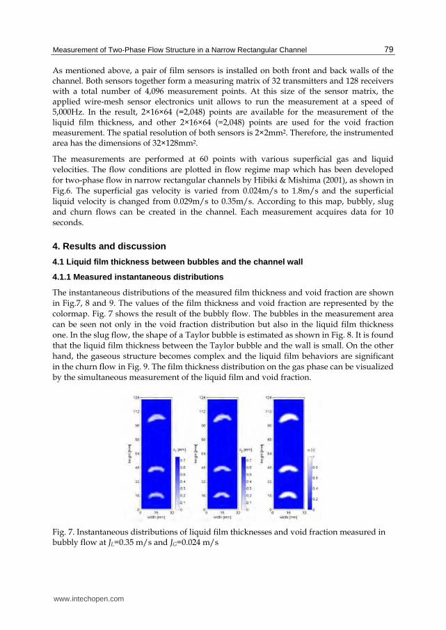
4.1.1 Measured instantaneous distributions

The instantaneous distributions of the measured film thickness and void fraction are shown

in Fig.7, 8 and 9. The values of the film thickness and void fraction are represented by the

colormap. Fig. 7 shows the result of the bubbly flow. The bubbles in the measurement area

can be seen not only in the void fraction distribution but also in the liquid film thickness

one. In the slug flow, the shape of a Taylor bubble is estimated as shown in Fig. 8. It is found

that the liquid film thickness between the Taylor bubble and the wall is small. On the other

hand, the gaseous structure becomes complex and the liquid film behaviors are significant

in the churn flow in Fig. 9. The film thickness distribution on the gas phase can be visualized

by the simultaneous measurement of the liquid film and void fraction.

Fig. 7. Instantaneous distributions of liquid film thicknesses and void fraction measured in bubbly flow at JL=0.35 m/s and JG=0.024 m/s

www.intechopen.com

Flow Measurement

80

Fig. 8. Instantaneous distributions of liquid film thicknesses and void fraction measured in slug flow at JL=0.17m/s and JG=0.22m/s

Fig. 9. Instantaneous distributions of liquid film thicknesses and void fraction measured in churn flow at JL=0.058m/s and JG=1.8m/s

When the bubble larger than the measurement volume comes between the electrodes

opposing each other, the electrical conductance in the gap should be almost zero. So the

measured void fraction is 100% at the point. However, the actual void fraction differs from

the measured value because of the existence of the liquid film layer. For example, when the

liquid film thicknesses are 150μm on the both walls and the local void fraction obtained

from the conductance is 100% at a given point, the actual void fraction in the narrow gap is

calculated as (s-├1–├2)/s = (1,500-2×150)/1,500 = 80%. As a result, there is a large difference

of 20%. This difference increases as the film thickness is larger. Thus, more accurate void

fraction estimation can be available by considering the liquid film thickness. This is

described in Section 4.2. In this study, the void fraction estimated from the electrical

conductance is used as a measure of bubble existence.

www.intechopen.com


81

0 8 16 24 320

100

200

300

400

500

Width [mm]

Film

th

ickn

ess

[m]

JG = 0.024m/s

0 8 16 24 32Width [mm]

JG = 0.22m/s

0 8 16 24 32Width [mm]

JG = 1.8m/s

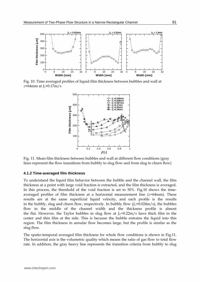
Fig. 10. Time averaged profiles of liquid film thickness between bubbles and wall at z=64mm at JL=0.17m/s

0.2 0.4 0.6 0.8 1

100

200

300

400

500

0 [-]

Film

th

ickn

ess

[m]

JL=0.029m/s JL=0.058m/s JL=0.087m/s JL=0.17m/s JL=0.26m/s JL=0.34m/s

Fig. 11. Mean film thickness between bubbles and wall at different flow conditions (gray lines represent the flow transitions from bubbly to slug flow and from slug to churn flow)

4.1.2 Time-averaged film thickness

To understand the liquid film behavior between the bubble and the channel wall, the film

thickness at a point with large void fraction is extracted, and the film thickness is averaged.

In this process, the threshold of the void fraction is set to 50%. Fig.10 shows the time-

averaged profiles of film thickness at a horizontal measurement line (z=64mm). These

results are at the same superficial liquid velocity, and each profile is the results

in the bubbly, slug and churn flow, respectively. In bubbly flow (JG=0.024m/s), the bubbles

flow in the middle of the channel width and the thickness profile is almost

the flat. However, the Taylor bubbles in slug flow at JG=0.22m/s have thick film in the

center and thin film at the side. This is because the bubble entrains the liquid into this

region. The film thickness in annular flow becomes large, but the profile is similar as the

slug flow.

The spatio-temporal averaged film thickness for whole flow conditions is shown in Fig.11. The horizontal axis is the volumetric quality which means the ratio of gas flow to total flow rate. In addition, the gray heavy line represents the transition criteria from bubbly to slug

www.intechopen.com

Flow Measurement

82

flow and from slug to churn flow. These criteria are obtained from the Hibiki-Mishima map shown in Fig.6. In bubbly flow with low volumetric quality, the film thickness is large because there are many small bubbles, which are located a bit far from the sensor surface. In addition, the thickness decreases as superficial gas velocity increases. The film thickness grows gradually in the transition from slug to churn flow. Furthermore, the thickness increases with superficial liquid velocity in slug and churn flows.

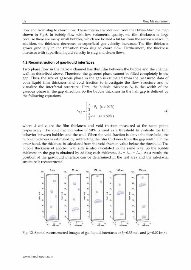
4.2 Reconstruction of gas-liquid interfaces

Two phase flow in the narrow channel has thin film between the bubble and the channel wall, as described above. Therefore, the gaseous phase cannot be filled completely in the gap. Thus, the size of gaseous phase in the gap is estimated from the measured data of both liquid film thickness and void fraction to investigate the flow structure and to visualize the interfacial structure. Here, the bubble thickness Δb is the width of the gaseous phase in the gap direction. So the bubble thickness in the half gap is defined by the following equations.

1

,1

( 50%)2

( 50%)2

b

s

s

(4)

where δ and ┝ are the film thickness and void fraction measured at the same point, respectively. The void fraction value of 50% is used as a threshold to evaluate the film

behavior between bubbles and the wall. When the void fraction is above the threshold, the bubble thickness is estimated by subtracting the film thickness from the gap width. On the

other hand, the thickness is calculated from the void fraction value below the threshold. The bubble thickness of another wall side is also calculated in the same way. So the bubble

thickness in the gap is obtained by adding each thickness, Δb = Δb,1 + Δb,2. As a result, the position of the gas-liquid interface can be determined in the test area and the interfacial

structure is reconstructed.

Fig. 12. Spatial reconstructed images of gas-liquid interfaces at JL=0.35m/s and JG=0.024m/s

www.intechopen.com


83



The typical images of the spatial reconstruction of the bubbly, slug and churn flows are

shown in Fig.12-14, respectively. In the bubbly flow, the three-dimensional bubble shape

and its variation can be found as shown in Fig. 12. The images of Taylor bubble are shown

in Fig. 13. The frontal and rear shapes of the bubbles can be seen. In addition, it is shown

that the gaseous phase and the liquid film behaviors are observed in the churn flow in

Fig.14. From these results, three-dimensional structures of the flow can be visualized by

reconstructing the interfaces.

4.3 Void fraction and interfacial area concentration

In gas-liquid two-phase flow, the void fraction and interfacial area concentration is

important to represent the flow characteristics. Thus, these parameters are estimate from the

measured data. As stated above, the void fraction measured from the electrical conductance

doesn’t involve the effect of film thickness behavior. Therefore, the void fraction in the gap

is recalculated from the bubble thickness as

www.intechopen.com

Flow Measurement

84

,1 ,2b b b

s s (5)

where s is the gap width.

0 1 2 3 4 50

0.2

0.4

0.6

0.8

1

Time [s]

[-]

(a) Bubbly flow at JL=0.35m/s and JG=0.024m/s

0 1 2 3 4 50

0.2

0.4

0.6

0.8

1

Time [s]

[-]

(b) Slug flow at JL=0.17m/s and JG=0.22m/s

0 1 2 3 4 50

0.2

0.4

0.6

0.8

1

Time [s]

[-]

(c) Churn flow at JL=0.058m/s and JG=1.8m/s

Fig. 15. Time-series profiles of the cross-sectional averaged void fraction for bubbly, slug and churn flows

The time-series profiles of the cross-sectional averaged void fraction are shown in Fig. 15. The void fraction has a peak when the bubble passes through the test section, as shown in Fig. 15 (a). In the result of slug flow, the length and passing frequency of bubbles can be found. The void fraction doesn’t reach 100% in even churn flow because the liquid film thickness is large. However, the large variation of the void fraction is detected in churn flow.

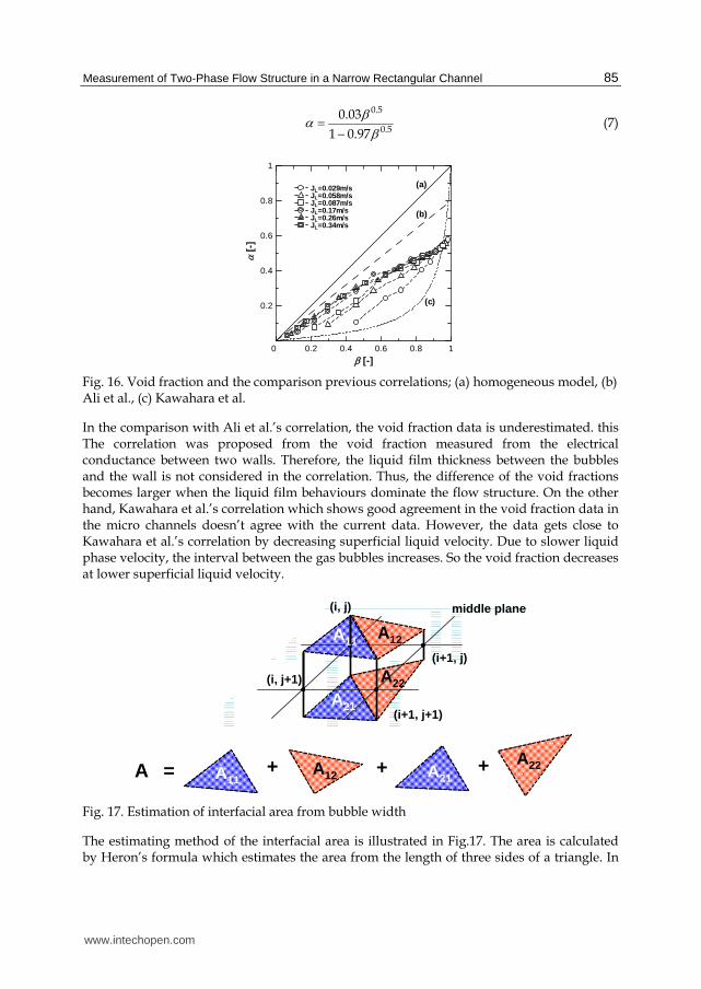
Fig.16 represents the void fraction data plotted against the volumetric quality for different superficial liquid velocity. The solid and dashed straight lines represent the homogeneous model (┙ = ┚) and Ali et al.’s correlation (Ali et al., 1993), respectively. The latter is expressed as follows,

0.8 (6)

This correlation was proposed for the narrow rectangular channels with gaps of 0.778 and 1.465mm. In addition, the dashed curve in Fig.16 is Kawahara et al.’s correlation (Kawahara et al., 2002) for circular micro channel with 100μm in diameter, as expressed in Eq.(7).

www.intechopen.com


85

0.5

0.5

0.03

1 0.97

(7)

0.2 0.4 0.6 0.8 1

0.2

0.4

0.6

0.8

1

0 [-]

[-]


(c)

(a)

(b)

Fig. 16. Void fraction and the comparison previous correlations; (a) homogeneous model, (b) Ali et al., (c) Kawahara et al.

In the comparison with Ali et al.’s correlation, the void fraction data is underestimated. this The correlation was proposed from the void fraction measured from the electrical conductance between two walls. Therefore, the liquid film thickness between the bubbles and the wall is not considered in the correlation. Thus, the difference of the void fractions becomes larger when the liquid film behaviours dominate the flow structure. On the other hand, Kawahara et al.’s correlation which shows good agreement in the void fraction data in the micro channels doesn’t agree with the current data. However, the data gets close to Kawahara et al.’s correlation by decreasing superficial liquid velocity. Due to slower liquid phase velocity, the interval between the gas bubbles increases. So the void fraction decreases at lower superficial liquid velocity.

+A = ++A11A12 A21

A22

(i, j)

(i+1, j)

(i+1, j+1)

(i, j+1)

A11A12

A21

A22

middle plane

Fig. 17. Estimation of interfacial area from bubble width

The estimating method of the interfacial area is illustrated in Fig.17. The area is calculated by Heron’s formula which estimates the area from the length of three sides of a triangle. In

www.intechopen.com

Flow Measurement

86

this estimation, four triangles are produced from four bubble thicknesses on each wall side, and the interfacial area formed by four measurement points is estimated as a sum of the area of their triangles. Then, the interfacial area concentration is calculated as

i

Aa

s x z (8)

where A is the area obtained in Fig.17, and Δx and Δz are the lateral and axial spacings between two measuring points, respectively.

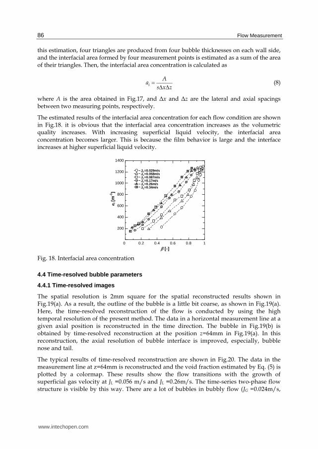
The estimated results of the interfacial area concentration for each flow condition are shown in Fig.18. it is obvious that the interfacial area concentration increases as the volumetric quality increases. With increasing superficial liquid velocity, the interfacial area concentration becomes larger. This is because the film behavior is large and the interface increases at higher superficial liquid velocity.

0.2 0.4 0.6 0.8 1

200

400

600

800

1000

1200

1400

0 [-]

a i [

m-1

]


Fig. 18. Interfacial area concentration

4.4 Time-resolved bubble parameters

4.4.1 Time-resolved images

The spatial resolution is 2mm square for the spatial reconstructed results shown in Fig.19(a). As a result, the outline of the bubble is a little bit coarse, as shown in Fig.19(a). Here, the time-resolved reconstruction of the flow is conducted by using the high temporal resolution of the present method. The data in a horizontal measurement line at a given axial position is reconstructed in the time direction. The bubble in Fig.19(b) is obtained by time-resolved reconstruction at the position z=64mm in Fig.19(a). In this reconstruction, the axial resolution of bubble interface is improved, especially, bubble nose and tail.

The typical results of time-resolved reconstruction are shown in Fig.20. The data in the measurement line at z=64mm is reconstructed and the void fraction estimated by Eq. (5) is plotted by a colormap. These results show the flow transitions with the growth of superficial gas velocity at JL =0.056 m/s and JL =0.26m/s. The time-series two-phase flow structure is visible by this way. There are a lot of bubbles in bubbly flow (JG =0.024m/s,

www.intechopen.com


87

JL =0.26m/s) and the detailed shape of Taylor bubble is estimated. In the spatial reconstruction, only the bubble less than the test area can be represented the whole bubble shape. However, even long Taylor bubbles are reconstructed in the time-series. In churn flow, the time variations of the gaseous structure and film behavior are found at JG =1.8m/s.

t = t1

t1

(a) (b)

x

y

z

xy

t

z = 64 mm

Fig. 19. Spatial and time-resolved reconstruction of Taylor bubble

To estimate the bubble size from the time-resolved data, the interfacial velocity is needed. Because the axial time axis has to be converted to spatial axis. If the interfacial velocity is assumed to be equal to the velocity of bubble, the individual bubble velocity can be used to estimate the bubble volume.

4.4.2 Bubble velocity

The cross-correlation method is applied to estimate the bubble velocity from the data. The schematics of the velocity estimation are shown in Fig. 21. For this estimation, the time-resolved void fraction data of two measurement line at different axial positions is used. In the void fraction distributions, the bubbles and liquid phase are separated by using a threshold of void fraction, and the bubbles are identified Therefore, the bubble travelling time ┬ between two lines is estimated by cross-correlating the void fraction data, and the bubble velocity is calculated by the following equation.

b

du (9)

where d is a distance between two measurement lines.

www.intechopen.com

Flow Measurement

88

50

12

34

Tim

e [s

]

JG=0.024m/sJG=0.15m/s

JG=0.58m/sJG=1.8m/s

50

12

34

Tim

e [s

]

JG=0.024m/sJG=0.15m/s

JG=0.58m/sJG=1.8m/s

JL=0.058m/s JL=0.26m/s

100%

0%

60%

20%

80%

40%

α

Fig. 20. Time-resolved images of the void fraction at z=64mm

d

z2

z1

01

Tim

e [s

]0.

20.

40.

60.

8

Time-resolvedvoid fraction distribution

z = z1 z = z2

τ1

τ2

τ3

Measurement section

width

Hei

ght

Fig. 21. Estimating method for individual bubble velocity with cross-correlation method

www.intechopen.com


89

0 1 2 3

ub [m/s]

JG=1.8m/s

0 1 2 3

ub [m/s]

JG=0.22m/s

0 1 2 30

0.2

0.4

0.6

0.8

1

ub [m/s]

PD

F [

-]

JG=0.024m/s

JL=0.058m/s

0 1 2 3

ub [m/s]

JG=1.8m/s

0 1 2 3

ub [m/s]

JG=0.22m/s

0 1 2 30

0.2

0.4

0.6

0.8

1

ub [m/s]

PD

F [

-]

JG=0.024m/s

JL=0.17m/s

0 1 2 3

ub [m/s]

JG=1.8m/s

0 1 2 3

ub [m/s]

JG=0.22m/s

0 1 2 30

0.2

0.4

0.6

0.8

1

ub [m/s]

PD

F [

-]

JG=0.024m/s

JL=0.35m/s

Fig. 22. Bubble velocity distributions for different flow conditions

0.2 0.4 0.6 0.8 1

1

2

0 [-]

ub [

m/s

]


Fig. 23. Mean bubble velocity (gray lines represent the flow transitions from bubbly to slug flow and from slug to churn flow)

www.intechopen.com

Flow Measurement

90

The probability density function (PDF) of the estimated bubble velocity at different flow conditions is shown in Fig.22. These results are broadly-divided into bubbly (left), slug (middle) and churn (right) flows. The profile has the pointed peak at low superficial gas velocity. When the superficial gas velocity increases, the peak moves to high velocity side and becomes smooth. In annular flow at JG =1.8m/s, the profiles are almost flat and there are many bubbles with higher velocity than 1.0m/s. It is also found that the bubble velocity increases as superficial liquid velocity increases in bubbly and slug flow. The mean bubble velocity is plotted against the volumetric quality in Fig.23. The bubble velocity at each flow regime depends on the superficial liquid velocity. At low superficial liquid velocity, the growth of the velocity with the volumetric quality is not so large in slug flow. In contrast, the bubble velocity at higher superficial liquid velocity increases greatly. The velocity in churn flow increases rapidly with the volumetric quality.

4.4.3 Bubble size

The bubble size of individual bubbles is estimated from time-resolved void fraction data and bubble velocity calculated above. The volume of bubble is calculated by integrating the local void fraction belonging to the bubble, as follows.

b bV s x t u (10)

where Δx is the lateral spacing between the electrodes and Δt is the time interval between two frames. The corresponding equivalent diameter is calculated using the volume as

36 b

eq

VD (11)

As a result, the bubble diameter for individual bubbles passing through the measurement line is obtained.

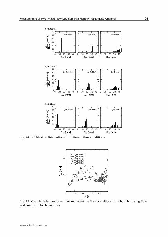
The bubble size distributions are presented in Fig.24. These distributions are at the same

flow conditions as the bubble velocity distributions in Fig.22. In the spatial reconstruction

of the bubble, the bubble size less than the measurement area can be estimated due to the

limitation of the area, i.e. Deq,max=22.7mm for 128×32×1.5mm3. However, the size of larger

bubble is obtained by the time-resolved reconstruction, as shown in Fig.24. In the results,

the bubble size increases with the increase of superficial gas velocity because of the flow

transition to slug and churn flow. Furthermore, the size decreases with the growth of

superficial liquid velocity in bubbly and slug flows. The bubble diameter is averaged and

the mean diameter for each flow condition is shown in Fig.25. The averaged bubble size

increases as the volumetric quality increases in bubbly flow. In slug flow, there is a large

difference of bubble size, since the number of bubbles is less during the measurement at

low superficial liquid velocity. Although more than 100 bubble are measured at high

superficial liquid velocity condition for 10 seconds, the sampled bubbles are only 6 at

JL =0.029 and JG =0.024m/s. Churn flow has not only huge bubbles but also many small

bubbles between large gas bubbles, and so the averaged value of the bubble size is not

so large.

www.intechopen.com


91

0 10 20 30 400

10

20

30

40

50

60

Deq [mm]

[%/m

m]

d

dD

eq

JL=0.058m/s

JG=0.024m/s

0 10 20 30 40

Deq [mm]

JG=0.22m/s

0 10 20 30 40

Deq [mm]

JG=1.8m/s

0 10 20 30 400

10

20

30

40

50

60

Deq [mm]

[%/m

m]

d

dD

eq

JL=0.17m/s

JG=0.024m/s

0 10 20 30 40

Deq [mm]

JG=0.22m/s

0 10 20 30 40

Deq [mm]

JG=1.8m/s

0 10 20 30 400

10

20

30

40

50

60

Deq [mm]

[%/m

m]

d

dD

eq

JL=0.35m/s

JG=0.024m/s

0 10 20 30 40

Deq [mm]

JG=0.22m/s

0 10 20 30 40

Deq [mm]

JG=1.8m/s

Fig. 24. Bubble size distributions for different flow conditions

0.2 0.4 0.6 0.8 1

10

20

0 [-]

Deq

[m

m]


Fig. 25. Mean bubble size (gray lines represent the flow transitions from bubbly to slug flow and from slug to churn flow)

www.intechopen.com

Flow Measurement

92

5. Conclusion

A novel measurement method for two-phase flow structure in narrow channel was described and an upwards air-water flow in a narrow gap was studied by the help of liquid film sensors. The liquid film thickness distributions between bubbles and the wall were determined on a two-dimensional domain and with high temporal resolution. The arrangement of sensors on both front and back walls of the test channel allowed measuring film thickness and void fraction simultaneously. Bubbly, slug and churn flows in a narrow rectangular channel with a gap of 1.5mm were measured and the characteristics of film behavior were investigated by averaging the thickness. The gas-liquid interfacial structure was reconstructed spatially by estimating the thickness of gaseous phase at each measurement point. Since the void fraction measured from the electrical conductance cannot be affected by the film behavior, the void fraction was recalculated from the spatial reconstructed data. In addition, the interfacial area concentration was also estimated from it. Finally, the time-resolved reconstruction was carried out in order to evaluate the bubble parameters (velocity and size), and the probability density function and time averaged quantities were estimated.

This technique can be applied to various flow channels such as the rod bundle geometries and micro capillaries. The measuring methods presented here offer the possibility to obtain data for the clarification of the multidimensional flow structure in a narrow channel. Furthermore, these data is also available for the validation of the CFD codes.

6. References

Ali, M.I., Sadatomi, M. & Kawaji, M. (1993). Adiabatic two-phase flow in narrow channels between two flat plates, The Canadian Journal of Chemical Engineering, Vol. 71, pp.657-666, ISSN: 0008-4034

Damsohn, M. & Prasser, H.-M. (2009). High-speed liquid film sensor for two-phase flows with high spatial resolution based on electrical conductance, Flow Measurement and Instrumentation, Vol.20, pp. 1-14, ISSN: 0955-5986

Damsohn, M. & Prasser, H.-M. (2010). Experimental studies of the effect of functional spacers to annular flow in subchannels of a BWR fuel element, Nuclear Engineering and Design, Vol.240, No.10, pp. 3126-3144, ISSN: 0029-5493

Fukaya, Y., Nakano, Y. & Okubo, T. (2009). Study on high conversion type core of innovative water reactor for flexible fuel cycle (FLWR) for minor actinide (MA) recycling, Annals of Nuclear Energy, Vol. 36, pp.1374-1381, ISSN: 0306- 4549

Han, Y. & Shilazono, N. (2009). Measurement of liquid film thickness in micro square channel, International Journal of Multiphase Flow, Vol.35, pp.896-903, ISSN: 0301- 9322

Hibiki, T. & Mishima, K., (2001). Flow regime transition criteria for upward two-phase flow in vertical narrow rectangular channels, Nuclear Engineering and Design, Vol.203, pp.117-131, ISSN: 0029-5493

www.intechopen.com


93

Ito, D., Prasser, H.-M., Kikura, H. & Aritomi, M. (2011). Uncertainty and intrusiveness of three-layer wire-mesh sensor, Flow Measurement and Instrumentation, Vol. 22, pp. 249-256, ISSN: 0955-5986

Ito, D., Kikura, H. & Aritomi, M. (2011). Micro-wire-mesh sensor for two-phase flow measurement in a narrow rectangular channel, Flow Measurement and Instrumentation, Vol.22, pp.377-382, ISSN: 0955-5986

Ito, D., Damsohn, M., Prasser, H.-M. & Aritomi, M. (2011). Dynamic film thickness between bubbles and wall in a narrow channel, Experiments in Fluids, Vol. 51, No.3, pp. 821-833, ISSN: 1432-1114

Iwamura, T., Uchikawa, S., Okubo, T., Kugo, T., Akie, H., Nakano, Y.& Nakatsuka T. (2006). Concept of innovative water reactor for flexible fuel cycle (FLWR), Nuclear Engineering and Design, Vol.236, pp.1599-1605, ISSN: 0029-5493

Kawahara, A., Chung, P.M.-Y. & Kawaji, M. (2002). Investigation of two-phase flow pattern, void fraction and pressure drop in a microchannel, International Journal of Multiphase Flow, Vol. 28, pp.1411–1435, ISSN: 0301-9322

Kawahara, A., Sadatomi, M. & Shirai, H. (2008). Two-Phase Wall and Interfacial Friction Forces in Triangle Tight Lattice Rod Bundle Subchannel, Journal of Power and Energy Systems, Vol.2, No.1, pp.283-294, ISSN: 1881-3062

Kureta, M. (2007). Development of a Neutron Radiography Three-Dimensional Computed Tomography System for Void Fraction Measurement of Boiling Flow in Tight Lattice Rod Bundles, Journal of Power and Energy Systems, Vol.1, No.3, pp.211-214, ISSN: 1881-3062

Kureta, M. (2007). Experimental Study of Three-Dimensional Void Fraction Distribution in Heated Tight-Lattice Rod Bundles Using Three-Dimensional Neutron Tomography, Journal of Power and Energy Systems, Vol.1, No.3, pp.225-238, ISSN: 1881-3062

Mishima, K, Hibiki, T & Nishihara, H. (1993). Some characteristics of gas-liquid flow in narrow rectangular duct, International Journal of Multiphase Flow, Vol.19, No.1, pp.115-124, ISSN: 0301-9322

Prasser, H.-M., Böttger, A. & Zschau, J. (1998). A new electrode-mesh tomograph for gas–liquid flows, Flow Measurement and Instrumentation, Vol.9, pp. 111-119, ISSN: 0955-5986

Sadatomi, M., Kawahara, A., Kudo, H. & Shirai, H. (2007). Effects of Surface Tension on Void Fraction in a Multiple-Channel Simplifying Triangle Tight Lattice Rod Bundle-Measurement and Analysis, Journal of Power and Energy Systems, Vol.1, No.2, pp.143-153, ISSN: 1881-3062

Tamai, H., Kureta, M., Ohnuki, A., Sato, T. & Akimoto, A. (2006). Pressure Drop Experiments using Tight-Lattice 37-Rod Bundles, Journal of Nuclear Science and Technology, Vol.43, No.6, pp.699-706, ISSN: 0022-3131

Uchikawa, S., Okubo, T., Kugo, T., Akie, H., Takeda, R., Nakano, Y., Ohnuki, A. & Imamura, T. (2007). Conceptual Design of Innovative Water Reactor for Flexible Fuel Cycle (FLWR) and its Recycle Characteristics, Journal of Nuclear Science and Technology., Vol.44, No.3, pp.277-284, ISSN: 0022-3131

Wong, H., Radke, C.J. & Morris, S. (1995). The motion of lung bubble in polygonal capillaries. Part 1. Thin films, Journal of Fluid Mechanics, Vol.292, pp.71-94, ISSN: 0022-1120

www.intechopen.com

Flow Measurement

94

Xu, J.L., Cheng, P. & Zhao, T.S. (1999). Gas-liquid two-phase low regimes in rectangular channels with mini/micro gap, International Journal of Multiphase Flow, Vol. 25, pp.411-432, ISSN: 0301-9322

www.intechopen.com

Flow MeasurementEdited by Dr. Gustavo Urquiza

ISBN 978-953-51-0390-5Hard cover, 184 pagesPublisher InTechPublished online 28, March, 2012Published in print edition March, 2012

InTech EuropeUniversity Campus STeP Ri Slavka Krautzeka 83/A 51000 Rijeka, Croatia Phone: +385 (51) 770 447 Fax: +385 (51) 686 166www.intechopen.com

InTech ChinaUnit 405, Office Block, Hotel Equatorial Shanghai No.65, Yan An Road (West), Shanghai, 200040, China

Phone: +86-21-62489820 Fax: +86-21-62489821

The Flow Measurement book comprises different topics. The book is divided in four sections. The first sectiondeals with the basic theories and application in microflows, including all the difficulties that such phenomenonimplies. The second section includes topics related to the measurement of biphasic flows, such as separationof different phases to perform its individual measurement and other experimental methods. The third sectiondeals with the development of various experiments and devices for gas flow, principally air and combustiblegases. The last section presents 2 chapters on the theory and methods to perform flow measurementsindirectly by means on pressure changes, applied on large and small flows.

How to referenceIn order to correctly reference this scholarly work, feel free to copy and paste the following:

Daisuke Ito and Horst-Michael Prasser (2012). Measurement of Two-Phase Flow Structure in a NarrowRectangular Channel, Flow Measurement, Dr. Gustavo Urquiza (Ed.), ISBN: 978-953-51-0390-5, InTech,Available from: http://www.intechopen.com/books/flow-measurement/measurement-of-two-phase-flow-structure-in-a-narrow-rectangular-channel-

measurement of two-phase flow structure in a narrow...

Documents