measurement-scheduled control for the …elghaoui/psfiles/dus98.pdf · measurement-scheduled...

INTERNATIONAL JOURNAL OF ROBUST AND NONLINEAR CONTROL

Int. J. Robust Nonlinear Control 8, 377—400 (1998)

MEASUREMENT-SCHEDULED CONTROL FOR THE RTACPROBLEM: AN LMI APPROACH

STEPHANE DUSSY* AND LAURENT EL GHAOUI

Ecole Nationale Superieure de Techniques Avancees, 32, Blvd. Victor, 75739 Paris, France

SUMMARY

The RTAC nonlinear control design benchmark problem is addressed using a multi-objective controlmethodology based on linear matrix inequalities and robust control. The approach hinges on the search fora common quadratic Lyapunov function ensuring various specifications (stability, L

2-gain, command input

and output peak bounds) for the closed-loop system. The resulting output-feedback controller is measure-ment-scheduled; precisely, its state-space matrices depend on the measurement vector, in a nonlinearfashion. We evaluate the performance of our design with various simulations and predicted trade-offcurves. ( 1998 John Wiley & Sons, Ltd.

Key words: linear matrix inequality; quadratic Lyapunov function; robust nonlinear control; linear-frac-tional representation; gain-scheduling

1. INTRODUCTION

1.1. Purpose

In this paper, we concentrate on a multicriteria nonlinear control problem, where a controller issought, such that a number of possibly conflicting constraints are met by the closed-loop system.

The paper is intended to serve two purposes. First, we seek to provide a tutorial on a systematicmethodology for multicriteria nonlinear control problems, recently developed in References1 and 2. Second, we illustrate this methodology on the RTAC benchmark problem introduced byBupp et al.3

Several approaches of the RTAC problem have been proposed in the past few years. Variousstabilization strategies are compared in Reference 4. Partial feedback linearization and integratorbackstepping methods are studied in References 5 and 6; adequate Lyapunov functions lead toa backstepping controller in Reference 7 and to a passive nonlinear controller in Reference 3.A state-feedback nonlinear controller is obtained in Reference 8, via the solution of a Hamilton—Jacobi—Isaacs equation.

Nonlinear control design is by itself a whole field of study, and a great variety of methods havebeen proposed: the second method of Lyapunov,9,10 exact linearization,11 extension of H

=methodology to nonlinear system,12~14 etc. Most of these techniques do not address multicriteria

*Correspondence to: Stephane Dussy, Ecole Nationale Superieure de Techniques Avancees, 32, Blvd. Victor, 75739Paris, France. E-mail: [email protected].

CCC 1049-8923/98/050377—24$17.50( 1998 John Wiley & Sons, Ltd.

problems directly. Furthermore, they may lead to equations that are hard to solve numerically, inparticular when output-feedback robust synthesis is involved. Finally, most of these approachesdo not take into account uncertainty, nor multiple specifications, explicitly.

The methodology proposed here is based on the search of a ‘common’ (quadratic) Lyapunovfunction for the closed-loop system, that guarantees the various design constraints simulta-neously.

Our choice of a common, quadratic Lyapunov function implies some degree of conservatism ofthe method. This disadvantage is traded-off against the numerical tractability of the resultingdesign algorithms. In fact, the method is a way to reformulate the control problem asone of choosing a few design parameters with direct physical interpretation (such as degreeof stability, L

2gain, etc.). (A more detailed discussion on common Lyapunov functions is in

Section 2.2.)It is, of course, possible to extend our approach to more elaborate (less-conservative) Lyapunov

functions, using, for example, parameter-dependent Lyapunov functions,15,16 integral quadraticconstraints,17 frequency-dependent multipliers,18 Lur’e-Postnikov-type functions19,20 or para-meterized Lyapunov bounds.21 However, most of these results only apply for robust analy-sis—they lead to very hard non-convex problems for robust synthesis. For example, attacking therobust synthesis problem with parameter-dependent Lyapunov functions leads to a set of bilinearmatrix inequalities (BMIs).

In contrast, using quadratic Lyapunov functions allows a numerically easier solution tosynthesis problems. (Recall that our main objective is to have a systematic and numericallytractable method.)

Based on a ‘linear-fractional representation’22~24 of the open-loop nonlinear system, we userobust control approaches and linear matrix inequality (LMI) optimization.25 The method is anextension of the gain-scheduling approach of Packard,26,27 to systems with non-necessarilybounded nonlinearities. To obtain the controller, we must find a solution to a set of LMIconditions, assorted with (at most) one quadratic, non-convex constraint. Our formulationenables us to use a cone-complementarity linearization algorithm that has proved its efficiency inthe static output-feedback problem,28 and in several other nonlinear control problems, wherealternative (BMI-based) approaches fail.

1.2. Paper outline

In Section 2, we provide an overview on our methodology. We describe in Section 3 themathematical specifications for our control design problem and we state it in terms of linear-fractional representations (LFRs). LMI-based synthesis conditions are derived in Section 4. Thelinear-fractional representation of the RTAC benchmark system, as described in Reference 3, andrelated numerical results, are given in Section 5.

1.3. Notations

For a real matrix P, P'0 (resp. P*0) means P is symmetric and positive-definite (resp.positive-semi-definite); P1@2 denotes its symmetric square root. The notation diag(A, B) withA3Rp]q and B3Rm]n denotes the matrix

diag(A, B)"CA

0

0

BD

378 STEPHANE DUSSY AND LAURENT EL GHAOUI

( 1998 John Wiley & Sons, Ltd. Int. J. Robust Nonlinear Control 8, 377—400 (1998)

For a given integer vector r"[r1,2, r

n], r

i3N, i"1,2, n, we define the sets

D(r)"M*"diag (d1Ir1,2, d

nIrn) D d

i3R, i"1,2, nN

B(r)"MB"diag (B1,2,B

n) DB

i3Rr

i]r

i, i"1,2,nN

S(r)"MS3B(r) DSi'0, i"1,2, nN

G(r)"MG3B(r) D Gi#GT

i"0, i"1,2, nN

Finally, CoMv1,2, v

LN denotes the polytope with vertices v

1,2, v

L.

2. AN OVERVIEW OF THE METHODOLOGY

2.1. Principles

The basic problem we consider is to find a nonlinear controller for a given non-linear system,such that the closed-loop system meets a number of specifications. (We will be more precise aboutthe required assumptions later.) The method is based on LFRs, quadratic Lyapunov functionsand multicriteria robust control design.

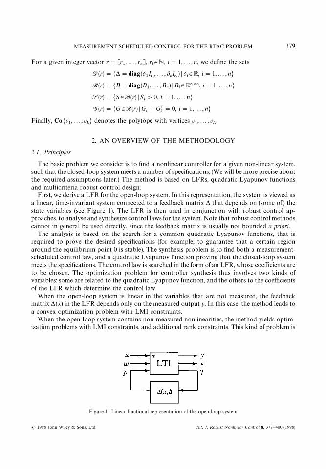
First, we derive a LFR for the open-loop system. In this representation, the system is viewed asa linear, time-invariant system connected to a feedback matrix * that depends on (some of ) thestate variables (see Figure 1). The LFR is then used in conjunction with robust control ap-proaches, to analyse and synthesize control laws for the system. Note that robust control methodscannot in general be used directly, since the feedback matrix is usually not bounded a priori.

The analysis is based on the search for a common quadratic Lyapunov functions, that isrequired to prove the desired specifications (for example, to guarantee that a certain regionaround the equilibrium point 0 is stable). The synthesis problem is to find both a measurement-scheduled control law, and a quadratic Lyapunov function proving that the closed-loop systemmeets the specifications. The control law is searched in the form of an LFR, whose coefficients areto be chosen. The optimization problem for controller synthesis thus involves two kinds ofvariables: some are related to the quadratic Lyapunov function, and the others to the coefficientsof the LFR which determine the control law.

When the open-loop system is linear in the variables that are not measured, the feedbackmatrix * (x) in the LFR depends only on the measured output y. In this case, the method leads toa convex optimization problem with LMI constraints.

When the open-loop system contains non-measured nonlinearities, the method yields optim-ization problems with LMI constraints, and additional rank constraints. This kind of problem is

Figure 1. Linear-fractional representation of the open-loop system

379MEASUREMENT-SCHEDULED CONTROL FOR THE RTAC PROBLEM


not convex; however an efficient heuristic, based on solving a sequence of LMI problems, can beused in this case.

There are several key features in the proposed approach.

f Efficient numerical solution. LMI optimization problems can be solved very efficiently usingrecent interior-point methods (the global optimum is found in modest computing item). Thisbrings a numerical solution to problems when no analytical or closed-form solution isknown.

f A systematic method. The approach is very systematic and can be applied to a very widevariety of nonlinear control design problems. This includes (and is not reduced to) systemswhose state-space representations are rational functions of the state vector.

f Extension to uncertain nonlinear systems. It is possible to extend the method to cases whensome parameters in the state-space representation of the system are uncertain.

f Multicriteria problems. The approach is particularly well suited to problems where several(possibly conflicting) specifications are to be satisfied by the closed-loop system. This is madepossible by use of a common Lyapunov function proving that every specification holds.

In view of the above features, the approach opens the way to CAD tools for the analysis andcontrol of nonlinear systems, see, e.g. the public domain toolbox MRCT29,30 built on top of thesoftware lmitool.31

2.2. Common Lyapunov functions in multicriteria design

Using the same Lyapunov function to enforce different specifications may lead to conservativeresults. This disadvantage is traded off in several ways.

First, other methods, such as H=

-control, do not allow to impose directly several constraints.One must form a single criterion, in the form of an H

=-norm bound, that is deemed to reflect all

specifications. Forming this one criterion may be difficult, since a (sometimes large) number ofparameters have to be chosen. Also, these design parameters do not always have obviousrelationship with the desired constraints.

In an LMI-based design, we form a set of LMI constraints, each one reflecting one specifica-tion. In each constraint appears a parameter that determines how coercive the specification is.Increasing the parameter amounts to relax the constraint. For example, if we impose an upperbound u

.!9on the command input norm, then u

.!9is a measure of how stringent the norm bound

is. The various parameters (command input u.!9

, L2-gain bound c, etc.) can be interpreted as

design parameters.In order to meet the specifications, the approach thus reduces the synthesis problem to

choosing a few design parameters. Note that all the design parameters have a direct physicalinterpretation, and that there is only a small number of them.

The possible conservatism of the LMI approach can be reduced if we choose the designparameters iteratively, as follows. At the first step of the design process, we may see the variousparameters to higher values than those imposed by the actual specifications. In a second step, wemay perform an (LMI-based) analysis, or a simulation, on the closed-loop system, in order tocheck if the latter obeys the specifications. (Since LMI-based design tools are more conservativethan LMI-based analysis tools, it seems that this will be often the case.) If not, we can identify(using analysis or simulation results) which specifications are violated, and modify the corres-ponding design parameters accordingly.



3. PROBLEM STATEMENT

3.1. Open-loop system

We consider a nonlinear, time-invariant, continuous-time system with a zero equilibrium point:

xR "A(d (x, t))x#Bu(d (x, t))u#B

w(d (x, t))w

y"Cy(d(x, t))x#D

yu(d(x, t))u (1)

z"Cz(d(x, t))x#D

zw(d (x, t))w

where x3Rn is the state vector, u3Rnu is the command input, w3Rnw is the exogenous input, z3Rnz

is the output of interest and y3Rny is the measured output. The vector-valued function d3RL isa nonlinear function of state x and time t.

We make the following assumptions.

A.1. A, Bu, C

y, C

z, D

yuand D

zware rational functions of their argument, that are well defined at

x"0.A.2. The function (x, t)Pd(x, t)3RL is Lipschitz, i.e. there exist constants M

1, M

2such that, for

every x, t, DDd (x, t) DD)M1DDx DD#M

2.

(Note that assumption A.2 can be relaxed).Using the methodology described in References 1 and 2, which we briefly recall in Appendix A,

we can derive from (1) an LFR for the system

xR "Ax#Buu#B

pp#B

ww

z"Czx#D

zpp#D

zuu#D

zww

y"Cyx#D

ypp#D

yuu#D

yww (2)

q"Cqx#D

qpp#D

quu#D

qww

p"*(x(t), t)q

where

*(x, t)"diag(d1(x, t)I

r1,2, d

L(x, t)I

rL)

and r"[r12r

L] is an integer vector (the element r

iis related to the highest degree of d

iin the

state-space functions of the system).With the above representation, the system is viewed as a feedback connection between an LTI

system and a (nonlinear) matrix * (x, t) (see Figure 1).For further reference, we now distinguish in the feedback matrix * the elements that are

measured in real time (we will label those meas, for ‘measured’), from those that are notmeasured (labelled unk, for ‘unknown’). Without loss of generality, we may assume that the firstM elements of d are measured:

* (x, t)"diag(*.%!4

(y), *6/,

(x, t))

where *.%!4

(y)"diag(d1(y)I

r1,2, d

M(y)I

rM) depends only on the measurement vector y.

For later reference, let l6/,

be the size of *6/,

, and l.%!4

be the size of *.%!4

. The total size of the* matrix is l"l

6/,#l

.%!4.



3.2. Controller structure

The controller structure is chosen to be ‘measurement-scheduled’, i.e.

xNQ "A1 (*.%!4

(y))xN #B1y(*

.%!4(y))y, xN (0)"0

u"CMuxN (3)

where xN is the controller state, CMuis a constant matrix and A1 , B1

yare rational functions of their

arguments di(y), i"1,2, M. (The term measurement-scheduled comes from the fact that, when

y is fixed, the above controller is linear time-invariant.) We shall also consider the case when thefull state is measured. In this case, our method will find a static, state-feedback control of the form

u"CMux

where CMu

is a constant matrix.Assuming that the matrix-valued functions A1 ( ) ), B1

y( ) ), etc. are rational functions of their

argument, we can always assume our measurement-scheduled controller to be in the LFR format:

xNQ "AM xN #BMyy#BM

ppN , xN (0)"0

qN "CMqxN #DM

qyy#DM

qppN

u"CMuxN (4)

pN "*.%!4

(y)qN

where pN and qN are fictitious inputs and outputs.We recall the crucial assumption here: the controller is scheduled with respect to the measured

element in the nonlinear block *, namely *.%!4

(y).

3.3. LFR of the closed-loop system

With the chosen controller structure, the closed-loop system assumes the form

xJ "A3 (*3 (x, t))xJ #B3w(*3 (x, t))w (5)

where xJ "[xT xN T]T. Here, A3 , B3w

are given rational functions of the nonlinearity element *3 , where

*3 (x, t)"diag(*.%!4

(y), *6/,

(x, t), *.%!4

(y)) (6)

Introducing

pJ "Cp

pN D, qJ "Cq

qN Dwe obtain the following LFR for the closed-loop system:

xJQ "(AI #BI KCIy#BI

uK

u)xJ #(BI

p#BI KDI

yp)pJ #(BI

w#BI KDI

yw)w

qJ "(CIq#DI KCI

y#DI

quK

u)xJ #(DI

qp#DI KDI

yp)pJ #(DI

qw#DI KDI

yw)w

(7)z"(CI

z#DI

zuK

u)xJ #DI

zppJ

pJ "*3 qJ , *3 (x, t)"diag (*.%!4

(y), *6/,

(x, t), *.%!4

(y))



Figure 2. LFR of the closed-loop system

where the matrices AI , BIp, etc., defined in Appendix B, depend affinely on the design matrix

variables CMu

and K. The closed-loop system is shown in Figure 2.In the above, the matrices CM

uand

K"CAMCM

q

BMp

DMqp

BMy

DMqyD

are the design variables.

3.4. Control design specifications

Typical specifications in a control design problem are

f The closed-loop system is stable over a given region containing 0.f The closed-loop system exhibits good settling behaviour for a class of initial conditions.f The closed-loop system exhibits good disturbance rejection compared to the uncontrolled

system for a class of disturbance signals.f The control effort should be reasonable.f Some output of interest z should not exceed a given level.

We now translate the above specifications in a mathematical form, which is defined in terms ofseveral ‘design parameters’.

First, to a given vector x0

with non-negative elements, we associate a region of admissibleinitial conditions, a polytope of the form

P(x0)"Co G C

$x0,1

F

$x0,nD H (8)

In the sequel, we denote by vj, j"1,2, 2n, the vertices of P (x

0). (It is possible to work with

ellipsoidal sets of initial conditions, such as P (x0)"Mx

0D DDx

0DD)1N.) We also consider the set of



admissible disturbances, chosen to be of the form

W (w.!9

)"Gw3L2([0R]) K P

=

0

w (t)Tw (t) dt)w2.!9H

where w.!9

is a given scalar.To the sets P (x

0) and W (w

.!9) we associate the set of ‘test trajectories’ for the closed-loop

system, i.e.

X(x0, w

.!9)"GxJ "C

x

xN D KxJ satisfies (5),

xN (0)"0, x (0)3P(x0), w3W(w

.!9)H

We introduce a vector x.!9

which will be used to bound the state variables (x.!9

is adesign parameter). We assume that the polytope P(x

0) (defined as in (8)) is included in

the polytope P (x.!9

); in other words, xi,0)x

i,.!9, i"1,2, n. Finally, let a, u

.!9and c be

positive scalars.Our design constraints are as follows.

S.1. The system is well posed, to be precise, the closed-loop system’s equations (5) are well definedfor every x3P(x

.!9).

S.2. Every trajectory in X(x0, 0) decays to zero at rate a, i.e.

limt?=

eatxJ (t)"0

S.3. For every trajectory in X (x0, w

.!9), the command input u satisfies

DDu (t) DD2)u

.!9for every t*0

S.4. For every trajectory in X (x0, w

.!9), the state is bounded componentwise, i.e.

Dxi(t) D)x

i,.!9for every i, 1)i)n and t*0

S.5. For every trajectory in X (0, w.!9

), and for every ¹*0, we have

PT

0

z (t)Tz(t) dt)c2PT

0

w (t)Tw(t) dt

where z is a given output.

Our final design depends obviously on the choice of the parameters x0, w

.!9, a, u

.!9, x

.!9and c. (Some of these parameters can be taken to be zero or infinite if the correspondingconstraint is void.) We stress that the design parameters are not necessarily those imposed by thespecifications.

The design parameters have obvious physical interpretations, and they may be adjusted ona heuristic basis. To this end, it is helpful to obtain trade-off curves between pairs of designparameters. For instance, in Section 5, we show curves of achievable performance (measured by c)versus control effort (measured by u

.!9), for various values of decay rate a.

The control design specification S.4 requires the state variables to be bounded componentwise.In view of assumption A.2, this will imply bounds on the matrix *. Note that these bounds are notnecessarily a priori bounds: they depend on the design parameter x

.!9.



4. SYNTHESIS CONDITIONS

4.1. Analysis via quadratic Lyapunov functions

We seek quadratic Lyapunov functions ensuring specifications S.1—S.5 for the closed-loop system. We thus consider a matrix PI 3R2n, with PI '0, and associated Lyapunovfunction

» (xJ )"xJ TPI xJ

Assume that, for a given non-zero trajectory in the set X (x0, w

.!9), » satisfies

»Q #2a»!c2wTw#zTz(0 (9)

The above inequality is at the basis of our control methodology. It obviously guaranteesspecification S.2. In addition, the above inequality also holds when a"0. Integrating both sidesof the resulting inequality yields

» (xJ (¹ ))#PT

0

z(t)Tz(t) dt)» (xJ (0))#c2PT

0

w (t)Tw(t) dt (10)

The above inequality guarantees S.5. Furthermore, it enables us to bound the state (or any linearcombination of it). For example, if x (0) is chosen such that

»(xJ (0)))j (11)

for some positive number j, then the corresponding trajectory satisfies

»(xJ (¹ )))j#c2w2.!9

. (12)

It suffices to ensure that inequality (11) holds at every vertex of the polytope of admissibleinitial conditions P(x

0), to obtain a bound on the resulting state vector that is valid for every

trajectory in X (specification S.4). We can use this inequality to bound the command input u, seenas a linear combination of the closed-loop system’s state (specification S.3). For more details onthis method, we refer to References 1, 2 and 25.

4.2. Related control strategies

Consider the following special cases of (9), namely,

»Q #2a»(0 (13)

and

»Q !c2wTw#zTz(0 (14)

We can outline two alternative control strategies related to the basic inequality (9).

f The switching strategy consists in designing two control laws: one is designed to guaranteea return to the vicinity of the equilibrium point in reasonable time, control effort and outputbounds despite disturbances, and is based on constraint (13). The other control law is on (14),and is designed to ensure a good disturbance rejection. The overall control law consists inapplying the first control until the state reaches a neighbourhood of x"0, then switching tothe other control law.



f The mixed strategy consists in designing one control law obeying to two requirements ofstability and disturbance rejection independently. This design is based on enforcing (13) and(14) simultaneously, with the same ».

The basic, switching and mixed all have advantages and drawbacks. The basic strategy mightbe more conservative than the two others, but it offers guarantees. In contrast, the (less-conservative) mixed strategy offers no guarantee, if the disturbance acts during a stabilizationphase. The switching strategy is even less conservative, but raises the additional problem ofestimating an appropriate switching time (this problem is easily dealt with if the full state ismeasured).

4.3. Matrix inequality conditions for analysis

In this section, we seek sufficient conditions guaranteeing that the closed-loop system satisfiesthe design specifications. To describe the basic principle, consider a nonlinear system

xR "A(* (x))x, * (x)"diag(x1,2,x

n) (15)

Assume we find a quadratic Lyapunov function »(x)"xTPx that guarantees robust stability ofthe associated uncertain system

xR "A (*(t))x, * diagonal, DD* (t) DD)1

If, in addition, this Lyapunov function proves that the output xisatisfies the bound Dx

i(t) D)x

i,.!9for every i and that these bounds imply DD* (t) DD)1 for every t*0, then the ellipsoid E

P"

Mx DxTPx)1N is a stable domain for system (15) (every trajectory initiating in EP

goes to zero).With the above basic principle in mind, we see that to guarantee our design specifications, it

suffices to write a robust stability (or more generally, robust performance) condition for anassociated uncertain system, associated with a condition that guarantees the state to be bounded.For more details, we refer to Reference 1.

In view of assumption A.2, we can always assume that DxiD)x

i,.!9implies some uniform bound

on the matrix *3 (x, t). To simplify, we assume that this bound writes DD*3 (x, t) DD)1. (We can alwaysuse loop transformations to end up with such a bound.)

The robust performance condition, derived from inequality (9), is that there exists a Lyapunovfunction matrix PI , and a scaling matrix SI commuting with any *3 of the form (6), such that

C2aPI #AI TPI #PI AI #CI T

qSI CI

qPI BI

p#CI T

zDI

zp#CI T

qSI DI

qpPI BI

w#CI T

qSI DI

qw* DI T

zpDI

zp#DI T

qpSI DI

qp!SI DI T

qpSI DI

qw* * DI T

qwSI DI

qw!c2ID(0 (16)

We note that the above inequality also guarantees well-posedness (specification S.1).The bound » (xJ (0)))j for every x (0)3P (x

0) can be written as

Cvj0D

TPI C

vj

0D)j, j"1,2,¸

With the above two conditions in force, we know that for every trajectory in X (x0, w

.!9),

inequality (12) holds. Specification S.3 then holds if

DD [O CMu]xJ DD

2)u

.!9for every xJ , xJ TPI xJ )(j#c2w2

.!9)



We rewrite the above condition as follows:

[O CMu]PI ~1[O CM

u]T)ku2

.!9I where k (j#c2w2

.!9)"1

Likewise, the output peak bound (specification S.4) then holds if

Cej0D

TPI ~1C

ej0D)kx2

j,.!9, j"1,2, n

where ejis the jth column of the n]n identity matrix.

4.4. Matrix inequality synthesis conditions

As seen in References 1 and 2, it is possible to formulate the synthesis conditions in the form ofLMI conditions associated with a non-convex constraint. These inequalities depend, in particu-lar, on P and Q, the upper-left n]n blocks of PI and PI ~1, respectively.

Let N be a matrix whose columns span the null space of [Cy

Dyp

Dyw

]T. The synthesisconditions are

& P, Q, S"CS.%!40

0

S6/,D, ¹"C

¹.%!40

0

¹6/,D3S(r)

j, k'0 and ½ such that

CP I

I QD*0, CS I

I ¹D*0 (17)

NT

ATP#PA#CTqSC

qPB

p#CT

qSD

qpPB

w#CT

qSD

qw

#2aP#CTzC

z#CT

zD

zp

* DTqp

SDqp!S DT

qpSD

qw

#DTzp

Dzp

* * DTqw

SDqw!c2I

N(0 (18)

AQ#QAT#Bu½#½TB

uQCT

q#½TDT

quQCT

z#½TDT

zu

#2aQ#Bp¹BT

p#c~2B

wBTw

#Bp¹DT

qp#c~2B

wDT

qwB

p¹DT

zp

* Dqp¹DT

qp!¹ D

qp¹DT

zp

#c~2Dqw

DTqw

* * Dzp¹DT

zp!I

(0 (19)

vTiPv

i)j, i"1,2,¸ (20)

Cku2

.!9I ½ 0

½T Q I

0 I PD*0 (21)

kx2j,.!9

!eTjQe

j*0, j"1,2, n (22)



and

S6/,

¹6/,

"Il6/,

, k (j#w2.!9

c2)"1 (23)

4.5. Solving for the conditions

Every condition above is an LMI, except for the non-convex equations (23). When (17) holds,enforcing this condition can be done by imposing Tr S

6/,¹

6/,#k(j#w2

.!9c2)"l

6/,#1 with

the additional LMI constraint

CkI

I

j#c2w2.!9D*0 (24)

In fact, the problem belongs to the class of ‘cone-complementarity problems’, which are basedon LMI constraints of the form

F (», ¼, Z)*0, C» I

I ¼D*0 (25)

where », ¼, Z are matrix variables (» and ¼ being symmetric and of same size), and F (», ¼, Z)is a matrix-valued, affine function, with F symmetric. The corresponding cone-complementarityproblem is

minimize Tr »¼ subject to (25).

The heuristic proposed in Reference 28, which is based on solving a sequence of LMI problems,can be used to solve the above problem. This heuristic is guaranteed to converge to a stationarypoint.

Cone complementarity algorithm H:

1. Find », ¼ and Z that satisfy the LMI constraints (25). If the problem is infeasible, stop.Otherwise, set k"1.

2. Find »k, ¼

kthat solve the LMI problem

minimize Tr(»k~1

¼#¼k~1

» ) subject to (25).

3. If the objective Tr(»k~1

¼k#¼

k~1»

k) has reached a stationary point, stop. Otherwise, set

k"k#1 and go to (2).

Depending on the number of measured and unmeasured parameters (related to the size ofmatrices *

.%!4and *

6/,, respectively, l

.%!4and l

6/,, we recover the previous results:

f If l6/,

"0 (there are no unmeasured nonlinearities), our conditions are convex, and equiva-lent to those obtained by Packard26 for gain-scheduling of LPVs. In this case, there is noneed to use the heuristic above.

f If l.%!4

"0 (there are no measured nonlinearities), our conditions are equivalent to theconditions obtained in robust synthesis based on quadratic stability.24

We note that, in the state-feedback case, the heuristic is not necessary and the problem isconvex. Note also that, in this case, the controller is linear. This is basically due to the use ofquadratic Lyapunov function, which implies a separation principle; in the output-feedback case,



the controller can be interpreted as a linear feedback u"KxL , where xL is the state estimated bya nonlinear observer.7

4.6. Controller reconstruction

When the algorithm exits successfully, i.e. when S6/,

¹6/,

KI and k (j#w2.!9

c2)K1 (note thata stopping criterion is proposed in Reference 28), then we can reconstruct an appropriatecontroller as follows.

First, we reconstruct a Lyapunov function for the closed-loop system » (xJ )"xJ TPI xJ , where PI iscomputed directly from the variables P and Q. When P'Q~1, the appropriate closed-loopLyapunov functions are parameterized by an arbitrary invertible matrix M3Rn]n, via theformula

PI "CI

0

0

MTD CP

I

I

(P!Q~1)~1D CI

0

0

MD (26)

(The choice of M is irrelevant: it corresponds to a change of coordinates of the controller’s states,xN PMx6 .) Similar formulae can be used to reconstruct an appropriate scaling matrix SI from thevariables S and ¹. We can also compute a controller matrix CM

ufrom the variables ½, P, Q, setting

CMu"½N~T, where N is the upper-right n]n block of PI ~1.Once a Lyapunov function PI and a scaling matrix SI is constructed, we proceed to reconstruct

the controller matrix K, as follows. We note that the controller gain matrix K (defined in Section3.3)) appears linearly in the analysis condition (16) when PI and SI are fixed. Therefore, we cancompute K by solving an LMI feasibility problem. Note that analytic controller formulae aregiven in Reference 32.

4.7. Overview of the design method

Our design method can be summarized as follows.

1. Describe the design problem mathematically, as in Section 3.4. Choose a set of designparameters a, u

.!9, x

.!9, etc.

2. Form an LFR of the open-loop system, and normalize it (use the design parameter x.!9

).3. Solve the synthesis conditions using algorithm H.4. If the design is satisfactory, reconstruct the controller and exit.5. Relax the design parameters and go to step 2.

We note that the method requires the parameters xi,.!9

to be finite if the corresponding statecoordinate x

iappears in the nonlinear element * (x).

The above method relies on an appropriate choice of the design parameters a, u.!9

, x.!9

, etc.This choice must be made on a heuristic basis. However, we stress that the designer has severalguidelines for this choice.

f Every parameter has an obvious physical interpretation, which helps deciding whether torelax, or strengthen, a given specification.

f The approach enables to compute trade-off curves. For example, we can compute theoptimal u

.!9attainable via the method, as a function of the decay rate a (the other parameters

being fixed).



5. NUMERICAL RESULTS

The numerical results were obtained using the public domain toolbox MRCT29,30 built on topof the software lmitool31 and the semidefinite programming package SP.33

5.1. The benchmark problem

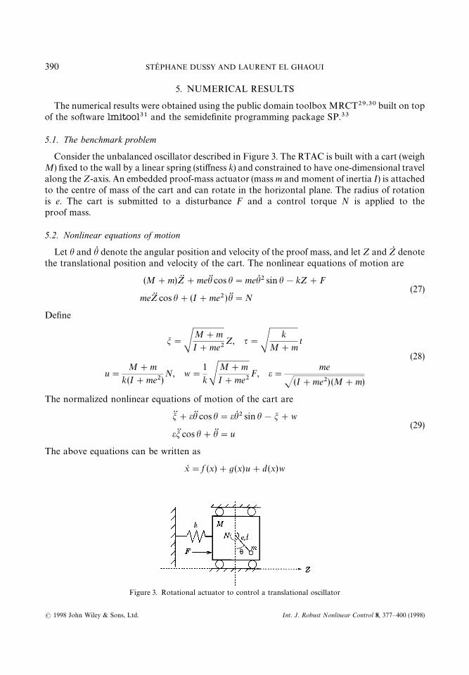
Consider the unbalanced oscillator described in Figure 3. The RTAC is built with a cart (weighM) fixed to the wall by a linear spring (stiffness k) and constrained to have one-dimensional travelalong the Z-axis. An embedded proof-mass actuator (mass m and moment of inertia I) is attachedto the centre of mass of the cart and can rotate in the horizontal plane. The radius of rotationis e. The cart is submitted to a disturbance F and a control torque N is applied to theproof mass.

5.2. Nonlinear equations of motion

Let h and hQ denote the angular position and velocity of the proof mass, and let Z and ZQ denotethe translational position and velocity of the cart. The nonlinear equations of motion are

(M#m)Z$ #meh$ cos h"mehQ 2 sin h!kZ#F(27)

meZ$ cos h#(I#me2)h$"N

Define

m"SM#m

I#me2Z, q"S

k

M#mt

(28)

u"M#m

k (I#me2)N, w"

1

kSM#m

I#me2F, e"

me

J(I#me2) (M#m)

The normalized nonlinear equations of motion of the cart are

m$#eh$ cos h"ehQ 2 sin h!m#w(29)

em$ cos h#h$"u

The above equations can be written as

xR "f (x)#g(x)u#d (x)w

Figure 3. Rotational actuator to control a translational oscillator



where the state is x"[m mQ h hQ ]T, and

f (x)"

x2

!x1#ex2

4sin x

31!e2 cos2x

3x4

e cos x3(x

1!ex2

4sinx

3)

1!e2 cos2x3

, g(x)"

0!e cosx

31!e2 cos2x

301

1!e2 cos2x3

, d (x)"

01

1!e2 cos2x3

0!e cosx

31!e2 cos2x

3

The measured outputs are m and h so that

yT"[m h]

Motivated by Biotras et al.,8 we choose the controlled output to be

zT"[J0)1m J0)1h u]

5.3. LFR model

In order to use the method, we need to work out an LFR model for the open-loop system. Tothis end, we choose a (state-dependent) ‘parameter vector’ d, such that the state-space equations ofthe system are linear when this parameter is frozen.

In the present case, we may choose d"[d1

d2], with

d1"cos x

3and d

2"x

4sin x

3

This choice leads to state-space equations of the form (1), with

A(d)"

0 1 0 0

!

1

1!e2d21

0 0ed

21!e2d2

10 0 0 1

ed1

1!e2d21

0 0 !

e2d1d2

1!e2d21

Bu(d)"

0

!

ed1

1!e2d21

01

1!e2d21

and Bw(d)"

01

1!e2d21

0

!

ed1

1!e2d21

The next task is to form an LFR for the parameter-dependent matrix M(d)"[A(d) B

u(d) B

w(d)]. This task can be done using construction rules detailed in Appendix A. The

basic idea of this construction is to decompose the matrix M into sums of fractions where the



parameters appear with degree one. We first obtain

A(d)T

Bu(d)T

Bw(d)T

T

"A0

!12

0

!12

1

1#ed1

#

0

!12

0

12

1

1!ed1B

1

0

0

!ed2

ed1

!1

T

#

0 1 0 0 0 0

0 0 0 0 0 0

0 0 0 1 0 0

0 0 0 0 1 0

We note that the parameter d1

appears three times (with degree one) in the above expression,while d

2appears only once. Therefore, the matrix * (appearing in (2)) is

*"diag(d1I3, d

2)

With the above representation, we may rewrite the state-space equations of the RTAC as (2),where the non-zero matrices are

A"

0 1 0 0

!1 0 0 0

0 0 0 1

0 0 0 0

, Bu"

0

0

0

1

, Cq"

1 0 0 0

1 0 0 0

0 0 0 0

0 0 0 1

, Bw"

0

1

0

0

Bp"

0 0 0 0

e2

!e2

!e e

0 0 0 0

e2

e2

0 0

, Dqu"

0

0

1

0

, Dqp"

!e 0 e !e

0 e e !e

0 0 0 0

0 0 0 0

, Dqw"

!1

!1

0

0

Cz"J0)1

1 0 0 0

0 0 1 0

0 0 0 0

, Dzu"

0

0

1

, Cy"C

1 0 0 0

0 0 1 0D5.4. Control design specifications

Throughout this section, we have set the design parameter x.!9

to

x.!9

"[1)28 R 0)5 0)5]T

We note that the value of m.!9

"1)28 is imposed by the physical configuration of the system,3while the other output bounds concern the maximal angular values, h

.!9and hQ

.!9. Note that we

do not impose a bound on the state mQ . This is allowed, since the latter variable appears linearly inthe equations of motion.

5.5. A mixed control design

We have designed a state-feedback and an output-feedback controller for the system, based onthe mixed control design strategy described in Section 4.2.



We first seek a state-feedback controller for our system. Our design parameters are

a"0)02, c"10, x0"[0)5 0 0 0]T (30)

Since the problem is convex in this case, we have taken the additional degree of freedom tominimize the upper bound on command input u

.!9, subject to the remaining LMI constraint.

We have found the guaranteed bound u.!9

"0)4586, and the resulting state-feedback, staticlinear controller is u"CM

ux, where

CMu"0)1[1)20 0)76 !6)49 !7)05]

An output-feedback controller was synthesized, based on the same design parameters (30), butwith a relaxation process on u

.!9, x

.!9, a and c. The controller is given by the LFR (4), with gain

matrices

AM "

!2)82 !1)46 0)13 !100)81

!5)20 !6)84 !2)13 73)68

!2)97 !4)51 !1)91 !2)66

9)57 !10)40 12)28 !1166)03

, BMy"

22)22 !1042)92

!2)32 !1977)47

!29)92 !1318)11

!2236)06 1)34

BMp"0)01

!6)10 !247)25 !119)77

4)48 181)32 86)11

!0)21 !6)95 5)64

!11)87 !481)25 !233)35

, CMu"0)01

0)04

0)63

0)33

!46)43

CMq"0)01

0)02 0)38 0)20 !27)53

0)19 3)00 1)59 !219)72

!1)32 !7)80 !2)73 486)07

DMqy"0)01

!0)04 !0)18

!0)74 !1)97

!229)26 !379)94

, DMqp"0)01

0)03 1)29 0)61

!0)14 !5)46 !2)58

0)29 11)88 5)90

This control law has been computed on a Sparc 4 workstation. It required 20 s of CPU time and977 Mflops for the solution of the LMI conditions, and 17 s of CPU time and 3)05 Gflops for thecontroller reconstruction phase. It only required one iteration in the algorithm H.

We show in Figure 4 the Bode plots of the nominal controller with inputs h and m, and withoutput the command u.

Figure 5 describes the closed-loop behaviour in response to zero external disturbances(F(t),0) and a non-zero initial condition for both controllers. These plots show the actualquantities (without the normalization (28)), i.e. N in Nm, w in N, Z in m, h in rad, t in s. We cannote that the various bounds that were required are ensured, and that the settling time (around 7 sfor the worst-case initial condition) is satisfactory.

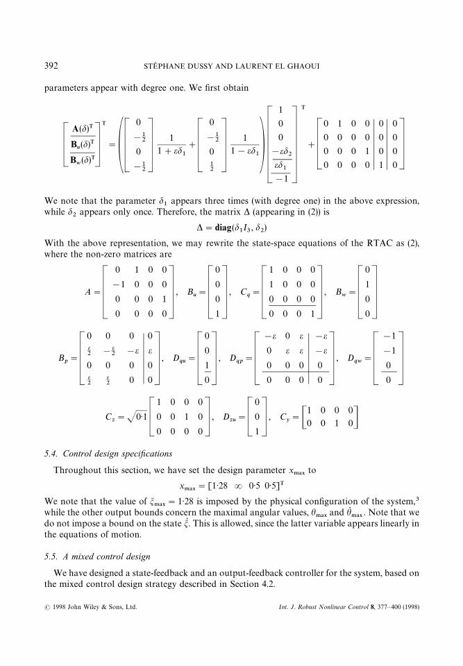
In Figure 6, we show the behaviour of the closed-loop system (with the output-feedbackcontroller), in response to an external disturbance F (t)"1)8 sin 10nt. The plots demonstrate how



Figure 4. Bode plots of the nominal output-feedback controller, with input m in plain line and with input h in dashed line

Figure 5. Closed-loop system time history with F(t),0, zero initial conditions except for Z (0)"0)023 m, for theoutput-feedback controller given in Section 5.5. t is in s, Z in m, h in rad and N in N



Figure 6. Open-loop (on the left) and closed-loop (on the right) system time history subject to zero initial condition anda non-zero external disturbance F(t)"1)8 sin 10nt, for the output-feedback controller given in Section 5.5. t is in s, Z in m

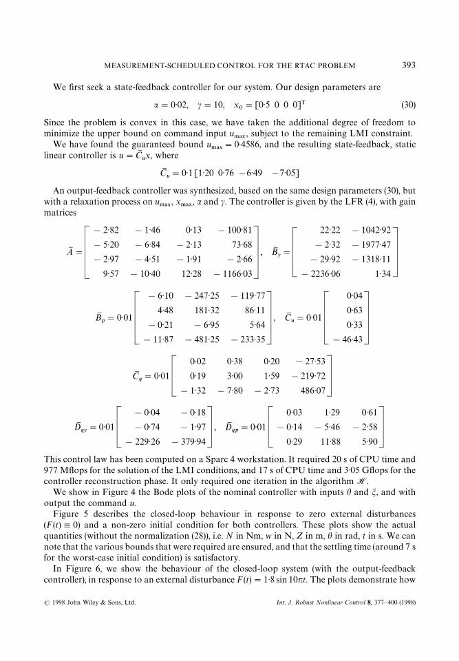
Figure 7. Open-loop (in dashed line) and closed-loop (in plain line) system time history subject to zero initial conditionand a non-zero external disturbance F(t)"sin 2nt, for the output-feedback controller given in Section 5.5. t is in s, h in rad

the system rejects the signal F (t). We also show the corresponding open-loop responses, whichturns out to be stable.

In Figure 7, we choose another disturbance signal F (t)"sin 2nt, that has a much lowerfrequency than the previous one. This time, the corresponding open-loop behaviour is unstable.In contrast, the controlled behaviour is still stable.

5.6. Some trade-off curves

It is interesting to compute predicted trade-off curves. Figure 8 shows trade-off curves decayrate/control effort, with c"R (right-hand side) and performance/control effort, with a"0(left-hand side). The design is based on the vector x

0given by (30). Performance is measured by c,

the upper bound on the closed-loop L2-gain and control effort is measured by the upper bound

on peak command input N.!9

. In each plot, two curves are shown: one for state feedback (in plainline) and the other for output feedback (in dashed line). Figure 9 shows similar results for the basic



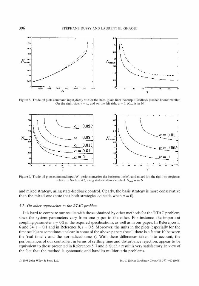
Figure 8. Trade-off plots command input/decay rate for the state- (plain line) the output-feedback (dashed line) controller.On the right side, c"R, and on the left side, a"0. N

.!9is in N

Figure 9. Trade-off plots command input/L2-performance for the basic (on the left) and mixed (on the right) strategies as

defined in Section 4.2, using state-feedback control. N.!9

is in N

and mixed strategy, using state-feedback control. Clearly, the basic strategy is more conservativethan the mixed one (note that both strategies coincide when a"0).

5.7. On other approaches to the RTAC problem

It is hard to compare our results with those obtained by other methods for the RTAC problem,since the system parameters vary from one paper to the other. For instance, the importantcoupling parameter e"0)2 in the required specifications, as well as in our paper. In References 5,6 and 34, e"0)1 and in Reference 8, e"0)5. Moreover, the units in the plots (especially for thetime scale) are sometimes unclear in some of the above papers (recall there is a factor 10 betweenthe ‘real time’ t and the normalized time q). With these differences taken into account, theperformances of our controller, in terms of settling time and disturbance rejection, appear to beequivalent to those presented in References 5, 7 and 8. Such a result is very satisfactory, in view ofthe fact that the method is systematic and handles multicriteria problems.



6. CONCLUSIONS

In this paper, we showed some key aspects of a methodology for nonlinear control introducedin Reference 1 and applied it to the RTAC benchmark problem. The approach can be adapted toa large class of nonlinear systems, and also to uncertain nonlinear systems,2 in particular, it is notrestricted to systems with bounded nonlinearities. It is very systematic and handles multicriteriacontrol. One important aspect of the method is that it allows computing trade-off curves formulticriteria design.

Recently, accurate robustness analysis tools based on multiplier theory have been devised, see,e.g. Megretsky and Rantzers17 and Balakrishnan.18 A complete methodology for nonlineardesign should include these tools for controller validation.

ACKNOWLEDGEMENTS

The authors wish to thank the Associate Editor and the anonymous reviewers for their precioushelp in improving the manuscript.

REFERENCES

1. El Ghaoui, L. and G. Scorletti, ‘Control of rational systems using linear-fractional representations and linear matrixinequlaities’, Automatica, 32, 1273—1284 (1996).

2. Dussy, S. and L. El Ghaoui, Multiobjective bounded control of uncertain nonlinear systems: an inverted pendulumexample, in Control of ºncertain Systems with Bounded Inputs, Springer, Berlin, 1997, pp. 55—73.

3. Bupp, R., D. Bernstein and V. Coppola, ‘A benchmark problem for nonlinear control design: problem state,experimental testbed, and passive nonlinear compensation’, Proc. IEEE American Control Conf., Seattle, WA, June1995, pp. 4363—4367.

4. Abed, E., Y.-S. Chou, A. Guran and A. Tits, ‘Nonlinear stabilization and parametric optimization in the benchmarknonlinear control design problem’, Proc. IEEE American Control Conf., Seattle, WA, June 1995, pp. 4357—4359.

5. Wan, C.-J., D. Bernstein and V. Coppola, ‘Global stabilization of the oscillating eccentric rotor’, Proc. IEEE Conf.Decision and Control, Orlando, FL, December 1994, pp. 4024—4029.

6. Bupp, R., C.-J. Wan, V. Coppola and D. Bernstein, ‘Design of a rotational actuator for global stabilization oftranslational motion’, Proc. ASME ¼inter Meeting, Vol. 75, Chicago, IL, 1994, pp. 449—456.

7. Kanallakopoulos, I. and J. Zhao, ‘Tracking and disturbance rejection for the benchmark nonlinear control problem’,Proc. IEEE American Control Conf., Seattle, WA, June 1995, pp. 4360—4362.

8. Tsiotras, P., M. Corless and M. Rotea, ‘An L2

disturbance attenuation approach to the nonlinear benchmarkproblem’, Proc. IEEE American Control Conf., Seattle, WA, June 1995, pp. 4352—4356.

9. Monopoli, R., ‘Synthesis techniques employing the direct method’, IEEE ¹rans. Automat. Control, 10, 369—370 (1965).10. Pomet, J.-B., R. Hirschorn and W. Cebuhar, ‘Dynamic output feedback regulation for a class of nonlinear systems’,

Math. Control Signals Systems 6, 106—124 (1993).11. Isidori, A., Nonlinear Control Systems: An Introduction, 2nd edn, Springer, Berlin, 1993.12. Van der Schaft, A., ‘L

2-gain analysis of nonlinear systems and nonlinear state-feedback H

=control’, IEEE ¹rans.

Automat. Control 37, 770—784 (1992).13. Isidori, A., ‘H

=control via measurement feedback for affine nonlinear systems’, Int. J. Robust Nonlinear Control, 4,

553—574 (1994).14. Lu, W. and J. Doyle, ‘H

=control of nonlinear systems: a convex characterization’, IEEE ¹rans. Automat. Control, 40,

1668—1675 (1995).15. Gahinet, P., P. Apkarian and M. Chilali, ‘Affine parameter-dependent Lyapunov functions for real parametric

uncertainty’, Proc. IEEE Conf. Decision and Control, Lake Buena Vista, FL, December 1994, pp. 2026—2031.16. Feron, E., P. Apkarian and P. Gahinet, ‘S-procedure for the analysis of control systems with parametric uncertainties

via parameter-dependent Lyapunov functions’, Proc. IEEE American Control Conf., Seattle, WA, June 1995, pp.968—972.

17. Megretski, A. and A. Rantzer, ‘System analysis via integral quadratic constraints’, Proc. IEEE Conf. Decision andControl, Orlando, FL, December 1994, pp. 3062—3067.

18. Balakrishnan, V., ‘Linear matrix inequalities in robustness analysis with multipliers’, Systems Control ¸ett., 25,265—272 (1995).



19. Haddad, W. and D. Bernstein, ‘Parameter-dependent Lyapunov functions and the Popov criterion in robust analysisand synthesis’, IEEE ¹rans. Automat. Control, 40, 536—543 (1995).

20. Sparks, A. and D. Bernstein, ‘Robust controller synthesis using scaled Popov bounds with uncertain A, B andC matrices’, IFAC 13th ¹riennal ¼orld Congress, San Francisco, LA, 1996, pp. 333—338.

21. Haddad, W., V. Kapila and D. Bernstein, ‘RobustH=

stabilization via parametrized Lyapunov bounds’, IEEE ¹rans.Automat. Control, 42 (2), 243—248 (1997).

22. Packard, A., K. Zhou, P. Pandey and G. Becker, ‘A collection of robust control problems leading to LMI’s’, Proc.IEEE Conf. Decision and Control, Brighton, England, December 1991, pp. 1245—1250.

23. Lu, W. and J. Doyle, ‘H=

control of LFT systems: an LMI approach’, Proc. IEEE Conf. Decision and Control, Tucson,AZ, December 1992, pp. 1997—2001.

24. Doyle, J., A. Packard and K. Zhou, ‘Review of LFTs, LMIs and k’, Proc. IEEE Conf. Decision and Control, Brighton,England, December 1991, pp. 1227—1232.

25. Boyd, S., L. El Ghaoui, E. Feron and V. Balakrishnan, ¸inear Matrix Inequality in Systems and Control ¹heory,SIAM, Philadelphia, PA, 1994.

26. Packard, A., ‘Gain scheduling via linear-fractional transformation’, Systems Control ¸ett., 22, 79—92 (1994).27. Becker, G. and A. Packard, ‘Robust performance of linear parametrically varying systems using parametrically-

dependent linear feedback’, Systems Control ¸ett., 23 , 205—215 (1994).28. El Ghaoui, L., F. Oustry and M. Aıt Rami, ‘A cone complementary linearization algorithm for static output-feedback

and related problems’, IEEE ¹rans. Automat. Control, (1997).29. Dussy, S. and L. El Ghaoui, ‘Multiobjective robust control toolbox for LMI-based control’, Proc. IFAC Symp.

Computer Aided Control Systems Design, Gent, Belgium, April 1997, pp. 353—358.30. Dussy, S. and L. El Ghaoui, Multiobjective Robust Control ¹oolbox (MRC¹): ºser’s Guide, 1996. Available via

http://www.ensta.fr/&gropco/staff/dussy/gocpage.html.31. El Ghaoui, L., R. Nikoukhah and F. Delebecque, ‘LMITOOL: A Front-End for ¸MI Optimization, ºser’s Guide,

February 1995. Available via anonymous ftp to ftp.ensta.fr, under /pub/elghaoui/lmitool.32. Iwasaki, T. and R. Skelton, ‘All controllers for the general H

=control problems: LMI existence conditions and state

space formulas’, Automatica, 30(8), 1307—1317 (1994).33. Vandenberghe, L. and S. Boyd, SP, Software for Semidefinite Programming, ºser’s Guide, December 1994. Available

via anonymous ftp to isl.stanford.edu under /pub/boyd/semidef—prog.34. Kinsey, R., D. Mingori and R. Rand, ‘Limited torque spinup of an unbalanced rotor on an elastic support’, Proc.

IEEE American Control Conf., Seattle, WA, June 1995, pp. 4368—4373.

APPENDIX A. LFR CONSTRUCTION

In this section, we provide some details about how an LFR model such as (2) can be constructed, fora parameter-dependent system (1).

Our framework includes the case when parameters perturb each coefficient of the state-space matrices ina (polynomial or) rational manner. This is due to the representation lemma given below.

Theorem A.1

For any rational matrix function M : R,PRn]c, with no singularities at the origin, there exist nonnegativeintegers r

1,2, r

p, and matrices M3Rn]c, ¸3Rn]N, R3RN]c, D3RN]N, with N"r

1#2#r

p, such that

M has the following LFR: for all d where M is defined,

M(d)"M#¸*(I!D*)~1R where *"diag (d1Ir1,2, d

LIrp) (31)

A LFR is thus a matrix-based way to describe a multivariable rational matrix-valued function. It isa generalization, to the multivariable case, of the well-known state-space representation of transfer functions(i.e. monovariable rational functions).

A constructive proof of the above result is based on a simple idea: first devise LFRs for simple (e.g. linear)functions, then use combination rules (such as multiplication, addition, etc.), to devise LFRs for arbitraryrational functions. To define the combination rules, we will start from two rational matrix-valued functionsof d3Rp, that are described in the LFR format:

Mi(x)"M

i#¸

i*i(I!D

i*i)~1R

i, i"1, 2

where *i"diag(d

1Iri

1,2, d

pIri

p), i"1, 2. In the sequel, we define *3 "diag(*

1, *

2).



Addition. The sum of M1

and M2

has the LFR

M(d)"M1(d)#M

2(d)"M#¸*3 (d) (I!D*3 (d))~1R

with

M"M1#M

2, ¸"[¸

1¸2], R"C

R1

R2D, D"diag(D

1, D

2)

Using row and column permutations, it is then possible to rewrite M(d) as in (31) (see the shuffling itembelow).

Multiplication. The product of M1(d) and M

2(d) is given by

M(d)"M1(d)M

2(d)"M#¸*3 (d) (I!D*3 (d))~1R

where

M"M1M

2, ¸"[¸

1M

1¸2], R"C

R1M

2R

2D, D"C

D1

0

R1¸2

D2D

Stacking. The combination of M1(d) and M

2(d) is

M(d)"[M1(d) M

2(d)]"M#¸*3 (d) (I!D*3 (d))~1R

with

M"[M1

M2], ¸"[¸

1¸2], R"diag(R

1, R

2), D"diag (D

1, D

2)

Shuffling. Suppose we are given a matrix function

M(d)"Ms#¸

s*s(d) (I!D

s*s(d))~1R

s

with *s(d) not necessarily in the required order (the variables may appear shuffled). Then, we can use row

and column permutations to put the above representation back into the LFR format. Precisely, takea permutation matrix E such that for every x,

ET*s(d)E"* (d)"diag(x

1Ir1,2, x

nIrn).

In this case, M(d) has the LFR

M(d)"M#¸* (d) (I!D*(d))~1R

where M"Ms, ¸"¸

sE, R"ETR

sand D"ETD

sE.

Inversion. If M is a square matrix with M(0) invertible, and has an LFR

M(d)"M#¸* (d) (I!D*(d))~1R

then its inverse can be written, for every d such that M(d) is invertible, as

M(d)~1"M~1!M~1¸*(d) (I!(D!RM~1¸)*(d))~1RM~1



APPENDIX B. LFR OF THE CLOSED-LOOP SYSTEM

The LFR of the closed-loop system is

xJQ "(AI #BI KCIy#BI

uK

u)xJ #(BI

p#BI KDI

yp)pJ #(BI

w#BI KDI

yw)w

qJ "(CIq#DI KCI

y#DI

quK

u)xJ #(DI

qp#DI KDI

yp)pJ #(DI

qw#DI KDI

yw)w

z"(CIz#DI

zuK

u)xJ #DI

zppJ

pJ "*3 qJ , *3 "diag(*l]l, *l.%!4]l.%!4

.%!4)

AI "CAn]n

0n]n

0n]n

0n]nD, BI "C0n]n

In]n

0n]nu

0n]nuD, BIu"C

Bn]nuu

0n]nuD

BIp"C

Bn]lp

0n]l0n]l.%!4

0n]l.%!4D, CIy"C

0n]n In]n

0l.%!4]n 0l.%!4

]n

Cny]ny

0ny]n DDI

qp"C

Dl]lqp

0l.%!4]l

0l]l.%!4

0l.%!4]l.%!4D, DI

yp"C

0n]l 0n]l.%!4

0l.%!4]l Il.%!4

]l.%!4

Dny]lyp

0ny]l.%!4 DDI

qu"C

Dl]nuqu

0l.%!4]nuD, CI

q"C

Cl]nq

0l.%!4]n

0l]n

0l.%!4]nD, DI "C

0l]n

0l.%!4]n

0l]l.%!4

Il.%!4]l.%!4D

BIw"C

Bn]nww

0n]nwD, DIyw"C

0n]nw

0l.%!4]nw

Dny]nwyw

D , DIqw"C

Dl]nwqw

0l.%!4]nwD

CIz"[Cnz]n

z0ns]n], DI

zu"Dnz]nu

zu, DI

zp"[Dnz]np

zp0nz]l.%!4]

K"CAM n]n

CM l.%!4]n

q

BM n]l.%!4p

DM l.%!4]l.%!4

qp

BM n]nyy

DM l.%!4]ny

qyD, K

u"[Onu]n CM nu]n

u]



measurement-scheduled control for the …elghaoui/psfiles/dus98.pdf · measurement-scheduled...

Documents