measurements of the average properties of a suspension of
TRANSCRIPT
J. Fluid Mech. (2001), vol. 429, pp. 307–342. Printed in the United Kingdom
c© 2001 Cambridge University Press
307
Measurements of the average propertiesof a suspension of bubbles rising
in a vertical channel
By R O B E R T O Z E N I T1,D O N A L D L. K O C H1 AND A S H O K S. S A N G A N I2
1School of Chemical Engineering, Cornell University, Ithaca, NY 14853, USA2Department of Chemical Engineering and Materials Science, Syracuse University,
Syracuse, NY 13244, USA
(Received 31 January 2000 and in revised form 6 September 2000)
Experiments were performed in a vertical channel to study the behaviour of amonodisperse bubble suspension for which the dual limit of large Reynolds numberand small Weber number was satisfied. Measurements of the liquid-phase velocityfluctuations were obtained with a hot-wire anemometer. The gas volume fraction,bubble velocity, bubble velocity fluctuations and bubble collision rate were measuredusing a dual impedance probe. Digital image analysis was performed to quantify thesmall polydispersity of the bubbles as well as the bubble shape.
A rapid decrease in bubble velocity with bubble concentration in very dilutesuspensions is attributed to the effects of bubble–wall collisions. The more gradualsubsequent hindering of bubble motion is in qualitative agreement with the predictionsof Spelt & Sangani (1998) for the effects of potential-flow bubble–bubble interactionson the mean velocity. The ratio of the bubble velocity variance to the square of themean is O(0.1). For these conditions Spelt & Sangani predict that the homogeneoussuspension will be unstable and clustering into horizontal rafts will take place.Evidence for bubble clustering is obtained by analysis of video images. The fluidvelocity variance is larger than would be expected for a homogeneous suspension andthe fluid velocity frequency spectrum indicates the presence of velocity fluctuationsthat are slow compared with the time for the passage of an individual bubble. Theseobservations provide further evidence for bubble clustering.
1. IntroductionHydrodynamic interactions and direct collisions between particles, drops, or bubbles
can have a dramatic effect on particulate and multiphase flows. Through the com-parison of careful experimental measurements with analytical theories and numericalsimulations, considerable progress has been made in the understanding of suspensionsin which viscous forces dominate on the particle length scale. The current understand-ing of the effects of particle interactions on inertial suspensions is much more limited.One type of inertial suspension, for which extensive theoretical work has been con-ducted, is a suspension of spherical, high-Reynolds-number bubbles. However, thereis a dearth of experimental measurements with which these theories can be compared.

308 R. Zenit, D. L. Koch and A. S. Sangani
The purpose of this paper is to present measurements of the flow properties of a nearlymonodisperse suspension of millimetre sized bubbles rising through water in a verti-cal channel. This system approximates the ideal conditions of high Reynolds numberand low Weber number that has been treated theoretically. We will also discuss thedevelopment of measurement protocols for suspensions of millimetre size bubbles.
The study of suspensions in which the inertia of the phases has a significanteffect is challenging and their treatment is, in general, more difficult than that oflow-Reynolds-number suspensions. There is a special case of an inertial suspensionthat is particularly amenable to theoretical analysis: a suspension of surfactant-free,spherical, high-Reynolds-number bubbles. In this case, the vorticity produced by thebubble motion is small (Moore 1963) and the fluid velocity can be expressed as thegradient of a potential obtained from solving Laplace’s equation. It is possible toderive, from first principles, equations of motion for this type of bubble suspension(Biesheuvel & Gorissen 1990; Sangani & Didwania 1993a; Zhang & Prosperetti1994; Bulthuis, Prosperetti & Sangani 1995; Kang et al. 1997; Spelt & Sangani 1998;Yurkovetsky & Brady 1996). In addition, dynamic simulations of many interactingbubbles can be conducted (Smereka 1993; Sangani & Didwania 1993b). The potentialflow approximation is applicable in the limits of high bubble Reynolds number andlow bubble Weber number. The Reynolds number is defined as Re = ρfdbub/µ, whereρf is the fluid density, db is the bubble diameter, ub is the relative velocity of the bubblewith respect to the fluid and µ is the fluid viscosity. The Weber number is definedas We = ρu2
bdb/σ, where σ is the surface tension of the liquid–gas interface. Theapplication of potential flow theory also requires that Marangoni effects be negligible,so that the tangential stress at the gas–liquid interface is small. Comparison betweenmeasured rise velocities for gas bubbles in water and theoretical predictions indicatethat the potential flow theory for spherical bubbles is reasonably accurate for bubblediameters of about 1 mm and the agreement between theory and experiment canbe improved by including the effects of bubble deformation (Moore 1965; Duineveld1995). Although the development of these theories represents a significant step towardsthe understanding of inertial suspensions, the extent of their applicability must becritically determined by comparison with experimental measurements.
There have been a large number of experimental studies that examine the behaviourof bubbly liquids since they are widely used in practical applications (Molerus &Kurtin 1985); however, most of the previous studies deal with the behaviour ofbubble columns in which the bubble size and polydispersity are neither small norcontrolled. These studies generally do not satisfy the dual limit of small Weber andlarge Reynolds number for which the potential flow theories may be applicable;therefore, direct comparisons are not possible. For bubbles rising under the action ofgravity, there exists a narrow range of bubble diameters for which this dual limit issatisfied. Bubbles of 1 mm in diameter rising in water move at approximately 30 cm s−1
in straight trajectories without shape oscillations and are close to spherical in shape.Another feature that makes the previous experimental studies deviate from the ideal
conditions for direct comparison with potential flow theories is the polydispersity ofthe bubbles which results, in part, from coalescence. In concentrated suspensions,coalescence often leads to a very wide distribution of bubble diameters that mayevolve over time. Coalescence can be prevented by the addition of salt to the liquidphase. Salt gives rise to short-range repulsive forces (known as hydration forces)between bubble interfaces which prevent coalescence. Lessard & Zieminski (1971)have shown that a sufficient concentration of salt in aqueous solution will preventcoalescence in bubble columns. Because the surface tension of the air–water interface

Measurements of bubble suspensions in vertical channels 309
is relatively insensitive to salt concentration, salt does not produce Marangoni effects(unlike organic surface active substances).
One previous study (Valukina, Koz’menko & Kashinskii 1979) used salt to preventcoalescence and thereby obtained a suspension of bubbles with diameters of 0.5–1 mm.In that study, the radial volume fraction profile was measured in an upward verticalpipe flow for dilute suspensions. In such a flow, lift forces drive bubbles towardsthe wall, while shear-induced bubble–bubble collisions may push bubbles toward thecentre of the pipe. The parameter regime explored by Valukina et al. was limited and inmany of the experiments the majority of the bubbles were concentrated in a layer thatwas about 1.5 bubble diameters thick near the tube wall. This makes it unlikely thatthe measurements can be compared with a continuum description of the suspension.Lammers & Biesheuvel (1996) performed experiments in a bubble column in whichthe bubble size variation was small to study the stability of concentration waves.With their experimental setup the bubble size variation was controlled; however, thesystem was not able to generate small enough bubbles to fall within the small Webernumber and large Reynolds number regime.
The experiment presented in this paper was designed to study a bubble suspensionwhich fulfilled as closely as possible the strict requirements for a direct comparisonwith the theories for bubble suspensions with potential flow interactions. While thepotential flow approximation has been shown to give a reasonably accurate descriptionof the rise of single bubbles (Moore 1965; Duineveld 1995), this study is the first tocritically examine its applicability to a suspension of bubbles rising due to buoyancy.Direct comparisons between theoretical and experimental results for the decrease ofthe mean bubble velocity with gas volume fraction are obtained. The discrepanciesfound are analysed and attributed to features that appear in the experiment and arenot accounted for in the currently available theories. In the experiment bubbles areslightly oblate and their aspect ratio changes as the gas volume fraction increases.The containing walls are found to have a significant effect, as bubbles experiencea decrease of velocity as a result of bubble–wall collisions. Also, bubble–bubbleand bubble–wall collisions cause bubbles to deform, introducing energy dissipationmechanisms not considered in current theories.
A distinctive feature that has been observed in the models and simulations ofbubbly liquids in potential flow is the appearance of horizontally oriented clusters ofbubbles (Smereka 1993; Sangani & Didwania 1993b). Bubble suspension images andthe spectrum of the liquid velocity produced by the bubbles are examined to provideevidence concerning the extent of bubble clustering in our suspensions.
Other mechanisms of clustering are known for bubbly liquids. Lammers & Biesheuvel(1996) observed clustering of bubble clouds as a result of concentration instabilitiesthat arise at sufficiently large bubble volume fractions due to the dependence of thedrag coefficient on bubble concentration. Lin et al. (1996) observed clustering andswirling bubble structures resulting from polydispersity of the bubble size. This is thefirst experimental study showing horizontal clustering due to potential flow for dilute,monodisperse systems.
This paper presents the experimental results obtained for a suspension of bubblesrising in water for which the Reynolds number is large, O(100), and the Weber numberis small, O(1). The device to generate the bubbles was designed to produce suspensionswith bubbles of approximately 1 mm in diameter and with small polydispersity. Animpedance probe, a hot-wire probe and video image processing were used to obtainmeasurements of the bubble size and shape, bubble velocity, bubble velocity variance,fluid velocity variance and bubble collision rate as functions of the mean bubble
310 R. Zenit, D. L. Koch and A. S. Sangani
High-speed camera
Nitrogen tankFlow meter
Controlvalve
200 cm
2 cm
20 cm
Capillaryarray
ProbeElectronics
Computer
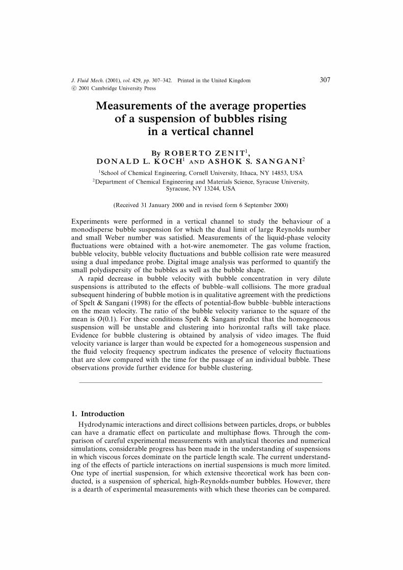
Figure 1. Experimental setup.
concentration. A detailed description of the instrumentation is provided. The resultsshow that the mean bubble velocity decreases as the bubble concentration increases,at a rate comparable to that predicted by Spelt & Sangani (1998). The fluid andbubble velocity variances are observed to increase with gas volume fraction.
In a companion paper, Zenit, Koch & Sangani (2000) present measurements of thegas volume fraction and liquid and bubble velocity profiles for a gravity-driven shearflow, in which the shear flow is generated by inclining the test channel a small anglewith respect to the vertical.
2. Experimental setupThe experiment is shown schematically in figure 1. The Plexiglas cell has a thickness
of 2 cm and a width of 20 cm. The thickness is chosen to obtain a near-continuumsuspension behaviour. The width is chosen so that the flow in the centre of thechannel is nearly two-dimensional. The cell height of 200 cm is large enough for thevelocity and volume fraction profiles to be fully developed. The channel is verticallyaligned within 0.1◦ using a digital level.
Nitrogen gas is introduced at the base of the channel through an array of capillaries.The capillaries are small enough to generate bubbles on the order of 1 mm in diameter,which satisfy the dual limit of small Weber number and large Reynolds number.The liquid phase is a dilute aqueous electrolyte solution (0.05 mol l−1 MgSO4). Theelectrolyte introduces a short-range hydration repulsion force between two gas–liquidinterfaces which inhibits bubble–bubble coalescence (Tsao & Koch 1994). Magnesium

Measurements of bubble suspensions in vertical channels 311
sulphate (MgSO4) was used because at very low concentrations it readily preventscoalescence (Lessard & Zieminski 1971). The addition of this small amount of saltdoes not change the viscosity or density of the liquid or the surface tension of thegas–liquid interface significantly.
The mean gas volume fraction, α, or hold up, is calculated by measuring the increasein liquid level after the bubbles are introduced to the cell,
α = (Ho/∆H + 1)−1 (2.1)
where Ho is the initial liquid level, and ∆H is the liquid level increase.High-speed video photographs and digital image processing are used to obtain
measurements of the bubble size and aspect ratio. Some measurements of the bubblevelocity are obtained using this technique but these are limited to the case of dilutesuspensions due to the opaque nature of bubbly fluids. Two types of probe areemployed to characterize the flow of the bubble suspension. A commercial hot-filmanemometer is used to measure the liquid velocity and the bubble–probe collision rate.A dual impedance probe was designed to measure the gas volume fraction, mean andfluctuating bubble velocities, the mean bubble chord length, and the bubble–probecollision rate. In this paper only bubble velocity results are presented.
2.1. Bubble generation
A device to produce the bubbly mixture was designed to keep the polydispersityof bubble diameter to the minimum possible. Capillaries with an inner diameter of100 µm were embedded in a perforated Plexiglas plate. Nearly 900 of these 65 mmlong tubes were positioned in a hexagonal array, in order to achieve the maximumnumber of tubes per unit of area (28 capillaries per square cm) without interferencebetween neighbouring capillaries. With this arrangement, the gas flow rate per tubewas small and the pressure drop across each tube was large. These two factors allowedthe bubble formation to occur in a quasi-steady fashion, resulting in the productionof uniform size bubbles (Og̃uz & Prosperetti 1993). The flow rate per capillary used inour experiments was always small enough so that the bubble size could be expectedto be independent of flow rate according to Og̃uz & Prosperetti’s criterion.
Figure 2 shows pictures of the bubbles produced for three typical mean gasconcentrations. The images were obtained by photographing the suspension throughthe 20 cm wall of the channel (the long dimension). The nearly monodisperse natureof the mixtures can be clearly observed. The mean bubble diameter is approximately1.4 mm. Also, some evidence of the clustering in bubble suspensions predicted bySpelt & Sangani (1999), Sangani & Didwania (1993) and Smereka (1993) can beobserved. More quantitative evidence for bubble clustering will be discussed in theexperimental results section.
The bubble size and aspect ratio were measured using digital image processing.The results are presented in the next section. The measurement error resulting fromthe finite pixel size of the digital images was calculated to be on the order of 3%.
2.2. Hot-film anemometry
A hot-film anemometer is used to measure the bubble–probe collision rate and theliquid fluctuating velocity in the bubble suspension. A sketch of the probe geometryis shown in figure 3. The hot-film probe used in the experiments consists of a 25 µmdiameter platinum wire coated with quartz to provide electrical insulation from theconducting liquid. The length of the sensitive part of the wire is 350 µm. The activewire is attached to the probe supports which are oriented perpendicular to the mean

312 R. Zenit, D. L. Koch and A. S. Sangani
(a)
(b)
(c)
Figure 2. Bubble size and distribution for typical mean gas volume fractions. The spacing in thegrid is 1 mm. (a) α = 0.02, (b) α = 0.05, (c) α = 0.10.

Measurements of bubble suspensions in vertical channels 313
1.5 mm
Probesupport
zvz
vy
vx
y
x
Sensitivewire
0.035 mm
Mean bubble motion
Figure 3. Sketch of the hot-wire probe and its orientation with respect to the mean bubble motion.
0.4
0.3
0.2
0.1
0 0.1 0.2 0.3 0.4 0.5 0.6 0.7 0.8 0.9 1.0
0 0.1 0.2 0.3 0.4 0.5 0.6 0.7 0.8 0.9 1.0
500
0
–500
Time (s)
Vel
ocit
y si
gnal
(m
s–1
)S
lope
of
velo
city
sig
nal (
m s
–2)
Figure 4. Typical fluid velocity signal and fluid velocity signal slope for a mean gas volumefraction of 0.05. The dashed line denotes the collision detection threshold level.
bubble motion to ensure that the same signal is detected for positive and negativevertical velocities. A typical velocity signal obtained from the hot-wire anemometerimmersed in the bubble suspension is shown in figure 4 along with the time derivativeof the velocity signal.
Hot-film probes have been used before for measurements of two-phase slug and

314 R. Zenit, D. L. Koch and A. S. Sangani
bubbly flows (Brunn 1995). However, most studies involved very high-speed flows withlarge bubble diameters. During the interaction of a large bubble with the probe at ahigh velocity, the probe is thought to pierce the bubble interface. In this study, usinghigh-speed photography, it has been observed that small bubbles (1–2 mm) movingat speeds comparable to their terminal velocity are not pierced by the anemometerprobe. Instead, the bubbles bounce off the probe. By synchronizing the velocity dataacquisition system with the high-speed camera, it was possible to observe that whena bubble collides with the sensitive part of the hot wire a sharp decrease of the slopeof the fluid velocity signal occurred. By analysing the sudden change in the signalslope when moving bubbles made contact with the hot wire, collisions were detectedand counted. An appropriate threshold level for bubble collision was determined byperforming experiments in which a single bubble was released at a series of differenthorizontal positions relative to the probe and the signal slope that occurred when abubble collided with the probe was noted. The minimum slope observed was differentfor direct collisions, grazing collisions and near-misses of the bubbles and the probe.By this procedure the cross-sectional area for bubble detection was measured to be1.803 mm2 for a bubble detection threshold level of −300 m s−2. A slight change inarea with threshold level occurs due to grazing collisions; however, it is clear that−300 m s−2 corresponds to a cut-off between direct hits and misses. Figure 4 showsthe collision detection level used in the experiments reported here as the dashed line.
The hot-wire anemometer responds primarily to velocity components perpendicularto the axis of the wire. The velocity signal obtained when the wire is parallel to animposed velocity is only 20% of that obtained when the wire is perpendicular to theflow. For simplicity, we will assume that the anemometer is measuring the projection ofthe velocity vector into the plane perpendicular the wire axis. Owing to the symmetryof the probe, the heat transfer from the wire is equal for upward and downwardflows relative to a horizontally oriented hot wire. Thus, the anemometer measures themagnitude
√v2x + v2
z of the fluid velocity perpendicular to the wire (y) axis. Thereforethe average of the fluid velocity signal illustrated in figure 4 is non-zero even thoughthe mean velocity is zero in a vertical channel. The velocity signal provides a measureof the fluctuations. By taking measurements with the hot wire oriented verticallyand horizontally, the variances of both the horizontal and vertical velocities can bedetermined.
2.3. Dual impedance probe
Impedance probes have been used widely by the multi-phase flow community tomeasure gas volume fraction (Ceccio & Georges 1996). However, in most cases suchtechniques are used to obtain a spatial average of the gas volume fraction across thethin dimension of the flow apparatus. The technique presented here can identify singlebubbles interacting with the measuring probe in a localized small measuring volume.This characteristic of the measuring system is needed to measure the spatial variationof the bubble concentration and velocity across the thin direction as will occur inour future investigation of inclined channel flows (Zenit et al. 2000). Impedancesystems able to measure and detect individual bubbles have been used only by a fewinvestigators (Waniewski 1999; Liu & Bankoff 1993).
The system can detect local changes of electrical impedance in bubbly mixtures.It uses the difference in electrical impedance between the gas and liquid phases todetermine the residence time of bubbles in a small measuring volume adjacent to theprobe tip. The probe arrangement is shown schematically in figure 5. An electrodeis embedded in a thin hypodermic needle, which acts as the ground. The electrode

Measurements of bubble suspensions in vertical channels 315
0.8 mm
0.6 mm
1.32 mm
Typical bubble sizeCross-sectional area for
bubble collision detection
Cross-sectional area forbubble velocity detection
Stainless steel hypodermic tubing (ground)
0.3 mm
Epoxy layer
Magnet wire (electrode)
Figure 5. Sketch of the dual impedance probe. The figure is drawn to scale.
carries a rapidly oscillating voltage. When bubbles pass near the tip of this probe, thelocal impedance and the current through the electrode are affected. The amplitude ofthe current signal is then converted to a DC voltage signal by an electronic circuit.The probes and electronic circuits used here are based on the design proposed byWaniewski (1999). A typical signal change detecting an individual bubble as it passesnear the tip of the probe is shown in figure 6.
In a vertical channel, the gas volume fraction can be determined simply by mea-suring the holdup (equation (2.1)). It is possible to measure the local gas volumefraction by establishing a voltage threshold level that discerns whether or not thereis a bubble in the vicinity of the tip of the probe. The vertical channel provides aconvenient setting in which to validate a volume-fraction measurement technique thatcan be used in more complicated situations where the volume fraction varies withposition. A detailed analysis of the performance of the impedance probe to measurelocal gas volume fraction is presented in the companion paper (Zenit et al. 2000). Forthis paper the gas volume fraction is obtained from the column holdup.
A second identical probe is positioned at a known distance above the leading probe.If a bubble passes near both probes, the signals produced in each of them will besimilar but shifted in time, as shown in figure 6. The signals are cross-correlated andthe delay time, τmax, can be accurately calculated as the value of signal shift time τthat maximizes the cross-correlation function, FV1V2
,
FV1V2(τ) =
1
ts
∫ ts
0
V1(t)V2(t− τ) dt (2.2)
where ts is sampling time and V1 and V2 are the voltages obtained from the leadingand trailing probes respectively. The bubble velocity can be obtained as
ub =D
τmax(2.3)

316 R. Zenit, D. L. Koch and A. S. Sangani
0.8
0.6
0.4
0.2
0
–0.20.25 0.26 0.27 0.28 0.29 0.30
Time (s)
Vol
tage
(V
)
Duration
Thresholdlevel
V1 V2
Figure 6. Typical voltage signal obtained from the impedance measurement resulting from a bubblepassing near the tip of the probe. The solid line denotes the signal obtained from the leading probe,the dashed line shows the signal from the trailing probe. The dotted line denotes the voltagethreshold level.
where D is the separation distance between probes. The velocity calculated in thismanner was compared with the velocity obtained using video image processing. Theresults differ only by 1% for a 1.3 mm bubble moving at 27 cm s−1. Note that forthis technique to be appropriate the bubble velocity must be nearly unidirectional,which is true for the flows studied in this paper. The bubble velocity calculatedfrom the cross-correlation function uses the entire time series (typically 100 s) fromthe impedance probe. The resulting measurement contains information from manydifferent bubble events.
Information concerning the probability distribution of bubble velocities can beobtained by further processing of the signals. A software program searches andidentifies voltage pulses corresponding to bubble detections by the leading probe, i.e.events for which the signal rises above the voltage threshold of 0.2 V. To determineif a similar pulse, shifted in time, was produced in the trailing probe, a local cross-correlation function is performed. A discriminating criterion is adopted to eliminateerroneous signals. If the calculated velocity is improbable, it is assumed that the signalsin the two probes were caused by two different bubbles and, therefore, the velocityis discarded. The algorithm discards velocities that are more than 50% larger thanthe terminal velocity and smaller than a tenth of the terminal velocity. In addition,events that yield small values of the maximum in the cross-correlation function,FV1V2
< 0.0015V 2, are discarded. The sample length used for the determination ofthe local cross-correlation function is 20 ms. In this way a set of individual velocitymeasurements is obtained, and therefore the variance of the vertical bubble velocity,Tb, can be determined.

Measurements of bubble suspensions in vertical channels 317
Different separations between the probes were tested. A distance of 1.32 mm wasused for the experimental results presented here. Larger distances resulted in poorcross-correlation values and shorter distances resulted in interference between theelectrical signals of the probes.
The calculations and the signal analysis are performed on the digitized voltagesfrom the probes. The sampling rate used was 10 kHz per probe, both for the impedanceprobes and the hot-wire system. The recording time per data point was, at least, 100 sfor all cases. The initial liquid height, Ho, was 1.50 m and was kept constant for allexperiments.
3. ExperimentsWith the instrumentation described above, precise measurements of the flow proper-
ties were obtained. Experiments were performed to determine the effect of gas volumefraction on the bubble collision rate, the mean and variance of the bubble velocity,and the fluid velocity variance. The range of gas volume fractions studied was from0 to 0.20. The size, size distribution and aspect ratio of the bubbles in the suspensionwere obtained as a function of gas volume fraction. Most of the measurements weretaken 100 cm above the bubble injector. However, a series of experiments confirmedthat the variation of the gas volume fraction with vertical position in the channel wassmall.
3.1. Single bubble experiments
A series of observations of single bubbles rising in a large pipe (20 cm in diameterand 40 cm in length) was conducted to determine the terminal velocity of a singlebubble of the same size as those produced in the channel. A single capillary, identicalto those used in the bank of capillaries to generate the bubble suspension, was usedto generate individual bubbles. Using video image processing, the terminal velocityof the bubble u∞ was found to be 0.320 m s−1 ± 3% with an equivalent diameterequal to 1.346 mm ± 3.5%. This results in a terminal Reynolds number of 431 anda Weber number of 1.969, assuming a value of 0.07 N m−1 for the surface tensionand a value of 0.001 Pa s for the liquid viscosity. The aspect ratio of the bubble was1.70±6%. The motion of the bubble was rectilinear and no bubble shape or trajectoryoscillations were observed. Based on Moore’s (1965) calculations, the rise velocity ofa bubble with the same equivalent diameter would be 0.317 m s−1, which is 0.9%lower than the experimentally measured velocity. The measurements of Duineveld(1995) show that for a bubble with the same equivalent diameter moving in purewater the terminal velocity is approximately 0.339 m s−1, 5.9% higher than the presentmeasurement. This discrepancy could be expected since in the present experiments thewater was deionized and filtered but the precautions used to assure purity were notas stringent as in Duineveld’s experiments. The measured aspect ratio is 11% higherthan the value predicted by Moore (1965), and 13% higher than the value measuredby Duineveld (1995) for the same value of Weber number. This discrepancy mayresult from deviations of the actual surface tension from the assumed value and/orfrom the existence of a small amount of impurities in the liquid.
3.2. Bubble size and aspect ratio
The mean and standard deviation of the equivalent diameter obtained from the imageanalysis are shown in figure 7, as functions of the mean gas volume fraction α. The

318 R. Zenit, D. L. Koch and A. S. Sangani
2.5
2.0
1.5
1.0
0.50 0.04 0.08 0.12 0.16 0.20
Mean gas volume fraction, α
Mea
n eq
uiva
lent
bub
ble
diam
eter
(m
m)
Figure 7. Equivalent bubble diameter, deq , as a function of mean gas volume fraction, α. The shortbars indicate the measurement error associated with the finite pixel size. The long bars indicate thebubble size standard deviation. The solid line depicts the linear fit shown in equation (3.2).
mean equivalent bubble diameter is calculated by
deq = (d2longdshort)
1/3 (3.1)
where dlong is the long axis length of the oblate bubble and dshort is the short axislength. For this measurement it is assumed that the bubble is axisymmetric withrespect to its short axis direction. The mean bubble size was found to increase slightlyfor gas volume fractions up to 0.20. The bubble size standard deviation, depicted bythe long bars, was approximately 10% and constant for gas volume fractions smallerthan 0.15. Note that, although the increase in the size of the bubbles is small, it has asignificant effect on the measurement of the gas volume fraction as discussed earlier.Coalescence of bubbles was not easily observable in the range of gas volume fractionsstudied here. However, the slight increase in bubble diameter may result from a smallamount of coalescence or from small changes in the size of the bubbles produced bythe capillaries with increasing gas flow rate. The variation of the equivalent bubblediameter with gas volume fraction can be approximated using the expression
deq = 1.66α+ 1.364 (3.2)
where the units of deq are mm. The statistical error associated with the size measure-ment is on the order of 3%.
Figure 8 shows the measurement of the bubble aspect ratio χ as a function of themean gas volume fraction, α. The aspect ratio is defined as χ = dlong/dshort. Note that

Measurements of bubble suspensions in vertical channels 319
1.8
1.6
1.4
1.2
1.0
0.80 0.04 0.08 0.12 0.16 0.20
Mean gas volume fraction, α
Bub
ble
aspe
ct r
atio
Figure 8. Bubble aspect ratio, χ, as a function of mean gas volume fraction, α. The bars indicatethe bubble aspect ratio standard deviation. Measurements obtained 50 cm above the bubbler. Thesolid line presents the prediction from equation (3.3).
the shape of the bubbles in the suspension is closer to spherical as the gas volumefraction increases. This results in part from the reduction of the mean rise velocityas the bubble concentration increases. The experimental results on the reduction ofthe mean terminal velocity are presented later in this section. Moore (1965) proposeda model to predict the bubble aspect ratio for slightly deformed bubbles moving inpotential flow, valid for moderate values of the Weber number in the absence ofbubble–bubble interactions. The implicit equation for the aspect ratio as a functionof the Weber number is
We(χ) = 4χ−4/3(χ3 + χ− 2)[χ2 sec−1 χ− (χ2 − 1)1/2]2(χ2 − 1)−3. (3.3)
Since the Weber number can be calculated from the present experiments as a functionof the bubble volume fraction, the change in bubble aspect ratio is obtained as afunction of gas volume fraction. The solid line in the plot shows the predicted aspectratio from equation (3.3). The bubble size change with gas volume fraction is takenfrom equation (3.2) and the decrease in bubble velocity is obtained from equation(3.4). The expression proposed by Moore does predict a decrease in the bubble aspectratio; however it underestimates the rapid decrease of the aspect ratio observed forgas volume fractions smaller than 0.05. This difference may arise as a result of thehydrodynamic interactions and collisions of bubbles with one another and with thewalls. Note also that the aspect ratio for a single bubble, χo = 1.7, presented inthe previous section, is higher than the measured aspect ratio even in very dilutesuspensions.

320 R. Zenit, D. L. Koch and A. S. Sangani
0.32
0.28
0.24
0.20
0.16
0 0.04 0.08 0.12 0.16
Gas volume fraction, α
Bub
ble
velo
city
(m
s–1
)
Figure 9. Bubble velocity as a function of mean gas volume fraction. The solid squares show themeasurements using the dual impedance probe. The lines show the predictions from Spelt & Sangani(1998) using u∞ = 0.320 m s−1 and different values of the parameter A: - - -, A = 10; – · –, A = 20;· · ·, A = A(α) from experiments shown in figure 10. The filled circle shows the terminal velocity of abubble moving in a large channel (u∞ = 0.320 m s−1). The empty circle shows the velocity measuredfor a single bubble in the experimental channel. The diamond shows the measurement for a verydilute suspension in the channel.
3.3. Bubble velocity and velocity variance
The measurements of the bubble velocity were obtained by placing the probe in thecentre of the channel where the velocity is nearly uniform. Measurements of thebubble velocity and bubble and fluid velocity variances were obtained for various gasvolume fractions. It was found that all the profiles are uniform across the channelwidth and changes in the profiles were only observed near the walls (Zenit et al.2000). Figure 9 shows the mean bubble velocity as a function of the gas volumefraction calculated from the column holdup. The mean bubble velocity decreases asthe bubble concentration increases.
From the measurement of the bubble diameter (equation (3.2)) and the meanbubble velocities (equation (3.4)) an experimental measure of the Reynolds andWeber numbers can be obtained. The Reynolds number is observed to decreasemonotonically with gas volume fraction from 380 for a dilute suspension to 260 for0.20 gas volume fraction. The Weber number also decreases with the gas volumefraction from 1.5 to 0.5 for the same range of gas volume fraction. The dual limit oflarge Reynolds number and small Weber number is therefore satisfied for this rangeof concentrations.
The bubble velocity measurements can be fitted approximately to the expression
ub = u∞(1− α)n (3.4)

Measurements of bubble suspensions in vertical channels 321
where n is an experimentally determined parameter and u∞ is the bubble velocity forthe limit of α→ 0. The fit of the experiments results in a value of n = 2.796 andu∞ = 0.269 m s−1. It is important to note that the value of n is larger than previouslyreported values for suspensions with comparable Reynolds numbers. Richardson &Zaki (1954) report a value of n = 2.5 for solid particles with a Reynolds numberof approximately 250 and Ishii & Zuber (1979) report a value of n = 2.0 for dropsand bubbles with the same range of Reynolds numbers. The reasons for this stronghindering behaviour are discussed below in § 3.3.2. Note also that the inferred valueof u∞ differs from the value measured for an individual bubble moving in a largepipe. Van Wijngaarden & Kapteyn (1990) observed a similar phenomenon for bubblesof approximately twice the diameter of the bubbles in this study. To investigate thecause of this apparent discrepancy, additional experiments were performed to studythe motion of individual bubbles in the test section.
For these experiments the bank of capillaries was replaced by an individual capillarywhere a single bubble could be formed. It was observed that the bubble moved atfirst in a straight trajectory, but after a certain distance (approximately 20 cm), itbegan to experience trajectory oscillations. The bubble moved diagonally from wallto wall, with a trajectory that differed slightly from the vertical direction. The bubblestranslated approximately three times the channel width in the vertical direction whilemoving from wall to wall. When the bubble came within one bubble diameter ofthe wall, it slowed its vertical velocity slightly, rotated, changed the direction ofits horizontal translation, and moved toward the opposite wall. This behaviour isdepicted schematically in figure 11 below. This translation from wall to wall resultedin a reduction of the mean bubble velocity as compared with that of a bubble ofthe same diameter moving in a large container. The mean velocity for this case was0.298 m s−1, and is shown in figure 9 denoted by the circle on the α = 0 axis. Thisvelocity, although smaller than the terminal bubble velocity, u∞ = 0.320 m s−1, is stilllarger than that inferred from the fit of the velocity measurements obtained with theimpedance probe. Note that in the case of a bubble moving in a large container nobubble trajectory oscillations were observed.
The mechanism behind this trajectory oscillation and how the bubble is repelledfrom the wall is not fully understood. A spherical bubble translating parallel to awall experiences an attraction towards the wall, resulting from the interaction withits image (its potential flow image to satisfy the boundary condition at the wall). Weobserved that oblate bubbles are first attracted to and then repelled by the wall. Thisbehaviour may result from the deformation of the bubble due to its interaction withits image. Duineveld (1994) performed experiments with interacting pairs of identicalbubbles rising side-by-side due to buoyancy and observed a similar phenomenon forlarge oblate bubbles. In that study two identical bubbles with equivalent diameterssmaller than 1.8 mm were observed to attract each other and interact repeatedly asthey moved. For bubbles with diameters larger than 2.04 mm the oblate bubbles wereobserved to interact initially and then separate permanently.
Figure 10 shows the measured bubble vertical velocity variance Tb normalized bythe square of the mean bubble velocity, u2
b, as a function of the gas volume fraction.The normalized variance increases with bubble concentration because the increas-ingly prevalent bubble–bubble hydrodynamic and collisional interactions increase thebubble velocity variance and decrease the mean of the bubble velocity. Along withthe experimental data, the lines show the values used for the comparisons with thepredictions of Spelt & Sangani in figure 9. The parameter A is the inverse of thenormalized bubble velocity variance which, for the comparison with the experimental

322 R. Zenit, D. L. Koch and A. S. Sangani
0.10
0.08
0.06
0.04
0.02
0 0.04 0.08 0.12 0.16
Gas volume fraction, α
Nor
mal
ized
bub
ble
velo
city
var
ianc
e, T
b/u
2 b
Figure 10. Normalized bubble vertical velocity variance as a function of mean gas volume fraction.The solid squares show the measurements using the dual impedance probe. The dashed and dash-dotlines represent the values of A used for the bubble velocity predictions for Spelt & Sangani (1998)in figure 9; the dotted line is the fit to the measurements. The circle shows the bubble velocityvariance measured for a single bubble in the channel. The diamond represents the bubble velocityvariance measured in a very dilute suspension.
measurements, only accounts for the vertical velocity variance. The dotted line showsthe fit to the experimental data. It is important to note that the variance does notapproach zero as the gas volume fraction tends to zero. From single bubble experi-ments in the channel, it was observed that bubbles underwent oscillating trajectoriesresulting from the bubble–wall interactions causing a decrease in the mean bubblevelocity and a bubble velocity variance. For a single bubble, the measured value ofthe normalized velocity variance is 0.0025, which is shown as a circle on the α = 0axis. The normalized variance resulting from the polydispersity of the suspensionwas calculated to be 0.001, which is even smaller than the variance produced by thebubble trajectory oscillations.
To further investigate the rapid change in the bubble velocity and velocity varianceas the concentration tends to zero, a series of experiments was performed in a verydilute suspension. Bubble concentrations smaller than α = 0.001 cannot be measuredaccurately. For such concentrations the increase in the height of the column resultingfrom the introduction of the bubbles is less than 1 mm, the minimum length thatcan be measured accurately. The impedance probe becomes inadequate for suchdilute systems since bubbles collide infrequently with the probe and the recordingtime required to obtain statistically significant results becomes impractical. Insteadthe bubble motion was determined from video images and the gas volume fractionregime will be henceforth referred to as ‘very dilute’.
In very dilute suspensions, the bubbles were observed to undergo oscillating tra-
Measurements of bubble suspensions in vertical channels 323
Single bubble Dilute mixture
Bubble-wallcollision
Lc
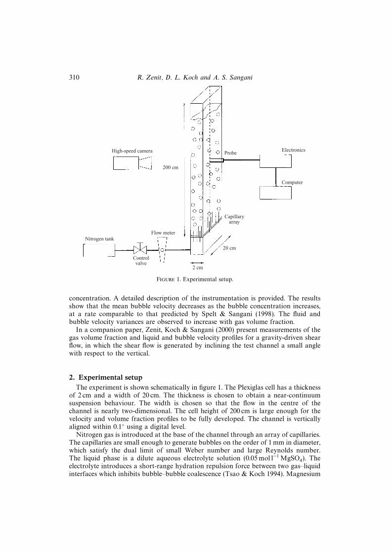
Figure 11. Schematic diagram of the motion of a single bubble in the channel and of a bubble in avery dilute suspension. Dashed lines indicate the presence of other bubbles in the suspension thatincrease the velocity fluctuations of the test bubble. Schematic is not to scale.
jectories. However, in contrast with the single bubble measurements, direct collisionsagainst the containing walls were observed in the very dilute suspension. During abubble–wall collision the bubble velocity decreases significantly, in accordance withthe observation of Tsao & Koch (1997). When colliding, the bubbles slowed down byas much as 75% of their original velocity and the shape of the bubble was alteredsignificantly. The velocity decrease as a result of the collision was calculated for anumber of bubble collisions. The ratio of the velocities after and before the collision,was 0.25 for the vertical component and 0.74 for the horizontal component.
As a result of the collisions with the containing walls in the very dilute suspension,the mean bubble velocity decreased to 0.288 m s−1 while the normalized bubblevelocity variance increased to 0.012 (denoted by the diamond symbols in figures9 and 10 respectively). These values are intermediate between the values obtainedfrom single bubble experiments and the suspension experiments with α > 0.01. Ina narrow region, at very low gas concentration, the bubble velocity and variancechange rapidly resulting from the bubble–wall collisions. Clearly the small increaseof gas volume fraction produced an increase in the bubble–bubble interactions whichresulted in large enough horizontal velocity fluctuations to cause bubbles to collidewith the containing walls. The collisions with the walls are, therefore, responsible forthe sudden decrease of the mean bubble velocity at very low concentrations. Figure11 depicts the observed behaviour schematically.
To corroborate the experimentally measured velocities a comparison can be per-formed between the superficial gas velocity, uo = Q/Ao, measured with the gas flowmeter and the product (ubα), of the holdup with the bubble velocity measured by theimpedance probe. Q is the volumetric gas flow rate and Ao is the cross-sectional areaof the channel. The correlation between the two measures is found to be very good,with no more than 5% discrepancy for all concentrations. At low concentration thegas flow measurements are slightly higher than the values measured directly with theimpedance probe but for more concentrated mixtures the measured bubble velocityis always larger than that calculated from the flow rate.
324 R. Zenit, D. L. Koch and A. S. Sangani
20
16
12
8
4
00.10 0.15 0.20 0.25 0.30 0.35
α = 0.010.020.050.10
Pro
babi
lity
den
sity
fun
ctio
n
Bubble velocity (m s–1)
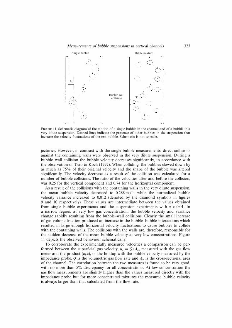
Figure 12. Normalized bubble velocity probability density function for four typical gas volumefractions. The width of the bins is 0.02 m s−1.
3.3.1. Probability density functions of bubble velocity
Probability density functions (PDFs) for the bubble velocity can be constructedfrom the individual measurements of bubble velocity. Figure 12 shows the PDFs forfour different mean gas volume fractions. All the PDFs are normalized such thatthe area under the curve equals one. For a dilute bubble suspension, the velocitydistribution is tall and narrow indicating that the velocity variance is small. As themean bubble concentration increases, the velocity distribution becomes wider. Themaximum of the PDF is observed to shift to lower velocities as the concentrationincreases in accordance with the mean bubble velocity measurements. Clearly, theshape does not appear to be truncated on either the high or low velocity sides, whichshows that the algorithm that discriminates erroneous signals is not eliminating realvelocity traces and, therefore, does not affect the results.
3.3.2. Comparison with theory
Spelt & Sangani (1998) derived the drag on a homogeneous suspension of sphericalbubbles rising through a fluid. Their result can be written in the form
ub =u∞(1− α)1 + 3
20αA
(3.5)
where A = u2b/Tb is the ratio of the mean bubble velocity squared to the bubble
velocity variance. Figure 9 shows the prediction from equation (3.5) for two constantvalues of the parameter A and using a function A(α) obtained from the fit of thevelocity variance measurements (from figure 10). The predictions are calculated usinga value of u∞ = 0.32 m s−1, corresponding to the single bubble moving in a largechannel. Despite the shift caused by the chosen value of u∞, the comparison is very

Measurements of bubble suspensions in vertical channels 325
good. The slope of the experimental curve is similar to that predicted by Spelt &Sangani. The primary difference between the experiment and the theoretical predictionis the rapid decrease in velocity with bubble concentration in the very dilute regime.As discussed above, we attribute this decrease to bubble–wall interactions which arenot included in the theory. It should also be noted that the values of A measuredin the experiments fall within the regime for which Spelt & Sangani predict that thehomogeneous suspension is unstable to cluster formation so that the applicability of(3.5) is uncertain.
The comparison of the theoretical and experimental results for the dimensionalmean bubble velocity shown in figure 9 does not take into account changes in theequivalent diameter and aspect ratio of the bubbles observed in the experiments. Tofactor out the changes in mean velocity that may arise due to these changes, the meanbubble velocity can be scaled with the terminal velocity uMoore predicted by Moore(1965) for an isolated bubble with the measured equivalent diameter deq and aspectratio χ, i.e.
uMoore =d2eqρfg
36µ
1
G(χ)(3.6)
where G(χ) is a function of the bubble aspect ratio, χ, given by
G(χ) = 13χ4/3(χ2 − 1)3/2 (χ2 − 1)1/2 − (2− χ2) sec−1 χ
(χ2 sec−1 χ− (χ2 − 1)1/2)2.
Using equation (3.2) and a fit of the experimental measurements of the bubble aspectratio, the terminal velocity for the oblate bubbles can be inferred as a function of thegas volume fraction. The normalized bubble velocity, ub/uMoore is shown in figure 13and is compared with expression (3.5) normalized by u∞,
ub
u∞=
(1− α)1 + 3
20αA.
Three different values of the parameter A were chosen: A = 10, A = 20 and a fit fromthe experiments, A(α).
As in the comparison of dimensional mean velocity given in figure 9, the theoryin figure 13 tends to overpredict the bubble velocity. The measured bubble velocityat zero bubble volume fraction is 5.5% lower than that calculated using Moore’sexpression. This difference may result from wall effects and possibly from small tracesof surface-active contaminants in our system. As the bubble concentration increases,the bubble diameter increases slightly and the bubble shape becomes nearly spherical.This leads to a significant increase in the terminal velocity uMoore. The experimentalmeasurements suggest that the trend toward more spherical bubbles with increasingbubble concentration does not decrease the drag force as much as might be expected.It should be noted that while the bubbles in the more concentrated suspensions arenearly spherical on average, they are constantly undergoing bubble–bubble collisionsthat excite small-to-moderate amplitude bubble shape oscillations. The dissipation ofenergy associated with these shape oscillations is one possible explanation for thehigher drag observed in the experiments as compared with the theory for perfectlyspherical bubbles. This possibility could be explored using numerical simulationsfor deformable bubbles with potential flow hydrodynamic interactions and directcollisions between the bubbles.
It is interesting to compare the change in the normalized mean velocity of thebubbles in our experiment with that predicted for other types of suspensions. At

326 R. Zenit, D. L. Koch and A. S. Sangani
1.0
0.9
0.8
0.7
0.6
0.5
0.4
0.3
0.20 0.04 0.08 0.12 0.16
Gas volume fraction, α
Nor
mal
ized
bub
ble
velo
city
, ub/u
Moo
re
ExperimentA = 10A = 20A = (α)
Figure 13. Normalized bubble velocity, ub/uMoore as function of gas volume fraction.
α = 0.18, the experimental measurements indicate a normalized bubble velocityof 0.25 compared with the prediction of 0.65 for spherical bubbles with potentialflow interactions, cf. figure 13. In fact the measured normalized bubble velocity iscomparable with the hindered settling velocity for a solid sphere in a low Reynoldsnumber flow (Durlofsky & Brady 1988; Ladd 1990). In addition to the role ofbubble deformation, another possible scenario that could lead to the large decrease innormalized bubble mean velocity observed in the experiments would be an increasein deviations from potential flow as the suspension becomes more concentrated. It isknown that the potential flow approximation provides an accurate description of therise of a single bubble (Moore 1965; Duineveld 1995), but much less is known aboutits accuracy in suspension flows. It is possible that the more complex flow patterns ina suspension and the cumulative effect of vorticity generation at many bubble surfaceslead to deviations from potential flow. It should also be noted that the case of bubblesrising steadily through a fluid would lead to larger deviations from potential flow thanwould occur in accelerating flows or flows with a larger ratio of the fluctuating tothe mean bubble velocity relative to the liquid. Noting that the drag on a single solidsphere at the lowest Reynolds number encountered in our experiments (Re = 280)is nearly four times larger than the drag on a spherical bubble in potential flow(Clift, Grace & Weber 1978), it can be seen that the deviations from potential flowwould not need to be extreme to lead to the decrease in bubble velocity observedexperimentally. As noted earlier the exponent in a Richardson–Zaki type correlationfor the bubble velocity (3.4) is larger (n = 2.796) in the present experiments thanRichardson & Zaki’s (1954) correlation for solid particles (n = 2.5) or Ishii et al.’scorrelation for drops and bubbles (n = 2.0). Ishii et al. do not specify whether theircorrelation corresponds to drops or bubbles and do not specify the Weber number.It is not surprising that the high Reynolds number, low Weber number bubbles

Measurements of bubble suspensions in vertical channels 327
exhibit stronger hindering than other types of suspensions. Bubbles in this specialtype of inertial suspension experience a very small O(12πµau∞) drag compared withthe O(ρa2u2∞) inertial drag characteristic of other high Reynolds number particles.Thus, the high Reynolds number, low Weber number bubble velocities are moresusceptible to decrease due to any new dissipation mechanisms that may arise due tobubble–bubble interactions.
Van Wijngaarden (1999) speculated that close interaction between moderateWeber number bubbles may lead to vortex shedding when a non-interacting bubblewould produce very little vorticity. This vortex shedding may enhance the drag in aconcentrated suspension considerably.
It should be noted that the video images used to determine the bubble diameterand aspect ratio in the more concentrated suspensions only probe the bubbles nearthe channel walls. Thus, it could be argued that the bubbles in the middle of thechannel may have a different size or aspect ratio than that measured by the imageanalysis. However, we do not believe that this effect is significant because we observedno statistically significant change in the mean bubble velocity and volume fractionmeasured by the impedance probe with position across channel gap.
3.4. Bubble–probe collision rate
Another quantity that can be used to characterize a bubble suspension is the bubblecollision rate. The collision rate quantifies the number of bubble events detected bythe probes per unit time. Unlike the measurement of bubble volume fraction by animpedance probe with a small measuring volume, the collision rate does not requirea consideration of the residence time of the bubbles in the measuring volume. In thissense, collision rate is a simpler quantity to measure. The collision rate can easily bepredicted from kinetic theories and is related to the volume fraction, mean velocityand velocity variance.
With the present experimental arrangement, the bubble collision rate can be de-tected using either the impedance or the hot-wire probe. The measurements can thenbe compared with each other by normalizing the collision rate by the cross-sectionalarea for bubble collision with the sensor’s sensitive area. The collision detection areais determined by the single bubble experiments in which bubbles were released atdifferent horizontal positions relative to the probe. The range of horizontal positionsfor which the probe signal rose above a specified threshold level was then determined.The sensitive area for the hot-wire probe was measured to be 1.803 mm2 for a velocityslope threshold level of −300 m s−2, and the sensitive area for the impedance probewas measured as a function of the bubble diameter as denoted by
Acoll = 0.611d2long − 1.588dlong + 1.747 (3.7)
where the units of dlong and the collision detection area are mm and mm2, respectively.This expression was obtained for a threshold level of 0.2 V.
Figure 14 shows the number of collisions per unit time per probe area as afunction of the mean gas volume fraction. The collision rate rises with increasingbubble number density as expected. The slope of the collision rate curve decreases asthe gas volume fraction increases. This results from the decrease in the mean bubblevelocity with gas volume fraction. The measurements from the two probes agreevery well for small bubble concentration but begin to differ for concentrations largerthan 0.05. This may result from differences in the nature of bubble interactions withthe two probes owing to differences in the probe geometries. The sensitive hot-wireprobe is supported by two posts (see figure 3) which may shield the probe from

328 R. Zenit, D. L. Koch and A. S. Sangani
14
12
10
8
6
4
2
0 0.04 0.08 0.12 0.16
Gas volume fraction, α
Nor
mal
ized
bub
ble
coll
isio
n ra
te (
s–1
mm
–2)
Figure 14. Number of collisions per unit time per probe area, or normalized collision rate, as afunction of mean gas volume fraction. The circles represent the measurements obtained with theimpedance probe normalized by the collision detection area from equation (3.7). The squares showthe measurements obtained with the hot film probe (aligned horizontally) normalized by a constantcollision detection area of 2.513 mm2. The dashed line is the prediction from equation (3.9).
collisions by bubbles with a significant horizontal velocity component. In contrastthe impedance probe (figure 5) restricts bubble collisions from a significantly smallerpart of angular space. The increasing velocity variance of the bubbles in moreconcentrated suspensions (illustrated in figure 14) may lead to more collisions frombubbles with larger horizontal velocity components that can be more easily detectedby the impedance probe.
Assuming that the bubbles all have the same velocity, the collision rate can beexpressed in terms of the bubble velocity, volume fraction and equivalent diameter as
Cr =6
π
αub
d3b
. (3.8)
Using equations (3.2) and (3.4), Cr can be calculated and compared with the directexperimental measurements.
Video image processing was used to evaluate the magnitude of the vertical andhorizontal bubble velocity variances. This technique, however, could only be usedwhen the bubble suspension was dilute. The ratio of vertical to horizontal bubblevelocity variance was measured to be 2.01 for a volume fraction of 0.005, and 1.75 fora volume fraction of 0.014. Clearly, the component of the bubble velocity variance inthe horizontal direction is smaller and has a small contribution to the bubble–probecollision rate. Hence, a more sophisticated estimate of the collision rate that takesaccount only of the fluctuations in the vertical bubble velocity can be obtained byassuming that the velocity takes on a Maxwellian distribution and has components

Measurements of bubble suspensions in vertical channels 329
only in the vertical direction:
fM(cz) =1
(2πTb)1/2exp
[−(cz − ub)2
2Tb
]where cz is the z-component of the bubble velocity. The collision rate can then beobtained by integrating
Cr =
∫nfM(cz)|cz| dcz
yielding
Cr =6α
πd3b
[√2Tbπ
exp (−u2b/2Tb) + ub(erf (ub/
√2Tb))
]. (3.9)
This expression can be evaluated using the measurements of the bubble volumefraction and the mean and variance of the bubble velocity and it is represented bythe dashed line in figure 14. The contribution of the velocity variance to the collisionrate obtained from equation (3.9) was found to be on the order of 0.01%.
The measurements from both probes deviate from the prediction for gas volumefractions greater than 0.05. The differences between the measured value of the collisionrate and the predictions may be an indication of the shielding produced by the probesupports.
3.5. Liquid velocity variance
The liquid velocity variance was determined from the hot-wire signal at various valuesof the mean gas volume fraction. The sensor was positioned in the middle of thechannel and measurements were taken with the probe axis oriented both horizontallyand vertically so as to obtain information concerning the vertical (Tfv) and horizontal(Tfh) velocity variances. As discussed in § 2.2, it is assumed that the probe signalresponds primarily to velocity components perpendicular to the probe axis. Thus, thesignal obtained when the probe is oriented vertically is a measure of 2Tfh and whenthe probe axis is horizontal Tfh + Tfv is measured.
Figure 15 shows Tfv and Tfh normalized by the square of the mean bubble velocityu2b as a function of the mean gas volume fraction. As expected, the liquid velocity
variance increases with gas volume fraction, since there are more bubbles to createfluid velocity disturbances . The vertical velocity variance is larger than the horizontalvelocity variance for all gas volume fractions as is usually the case in sedimentingsuspensions.
A prediction of the liquid velocity variance in a dilute suspension of homogeneouslydistributed bubbles can be obtained by calculating the potential-flow fluid velocityvariance produced by a single spherical bubble translating through an unboundedfluid. The potential function for a sphere of radius, a = db/2, moving at a velocity ubis given by
φ =1
2
a3
r3x · ub. (3.10)
The fluid velocities in the vertical and horizontal directions are calculated as
ux =∂φ
∂x, uy =
∂φ
∂y
where x, y, z are Cartesian coordinates with the x-axis parallel to gravity. To obtainthe fluid velocity variance, the square of the velocity disturbance is integrated over all

330 R. Zenit, D. L. Koch and A. S. Sangani
0.5
0.4
0.3
0.2
0.1
0 0.04 0.08 0.12 0.16
Gas volume fraction, α
Nor
mal
ized
flu
id v
eloc
ity
vari
ance
, Tf/u
b2
Figure 15. Normalized fluid velocity variance as a function of gas volume fraction. The solidsquares show the vertical velocity variance, Tfv , and the diamonds depict the horizontal velocityvariance, Tfh. The open squares represent the vertical velocity variance measured in the ‘very dilute’limit. The solid line shows the prediction of the vertical fluid velocity variance from equation (3.11),and the dashed line shows the horizontal fluid velocity variance from equation (3.12).
space and multiplied by the bubble number density,
〈u2x〉 = n
∫V
u2x dV ,
〈u2y〉 = n
∫V
u2y dV ,
yielding
〈u2x〉 = 1
5αu2
b, (3.11)
〈u2y〉 = 3
20αu2
b. (3.12)
The predictions from equations (3.11) and (3.12) are shown in figure 15 by thesolid and dashed lines, respectively. Both the theoretical predictions for a dilute,homogeneous suspension and the experimental measurements indicate that the verti-cal velocity variance is substantially larger than the horizontal. However, this simpletheory under-estimates the liquid velocity variance at all bubble concentrations.At the higher bubble concentrations, this discrepancy could result from the detailsof the bubble–bubble interactions that are neglected in the model. However, thelarge velocity variance in a dilute suspension suggests that the suspension may notbe homogeneous. Clusters of bubbles in a dilute suspension would be expected toproduce a larger liquid velocity disturbance than homogeneously distributed bubbles.This observation can be inferred from the simulation results of Sangani & Didwania(1993b), where the added mass coefficient was calculated and it was observed toincrease as the bubble clusters formed.

Measurements of bubble suspensions in vertical channels 331
The non-spherical nature of the bubbles also causes the liquid velocity variance tobe larger than that predicted for spherical bubbles. We can get an estimation of magni-tude of this effect by comparing the added mass coefficient (which is the kinetic energyof the liquid) for spherical bubbles to that for oblate spheroids resembling the bubblesin the experiments. For example, the added mass coefficient for an oblate spheroid ofaspect ratio 1.5 is 4/5, while that for a sphere is 1/2. Hence, in this case, the non-sphericity of bubbles would be expected to increase the velocity variance by 60% andthereby explain a small portion of the discrepancy between the theory and experiment.
Note that, as in the case of the measurement of the bubble velocity variance, thevertical liquid velocity variance appears to approach a finite value as the concentrationof bubbles approaches zero. A series of measurements was performed for the ‘verydilute’ limit in which the concentration cannot be measured accurately (shown by theopen squares in figure 15). It was found that the fluid velocity variance rapidly in-creases for that range of concentrations. One would expect the liquid velocity varianceto approach zero as α→ 0 in a homogeneous suspension. However, it will be seen inthe following section that the bubbles form clusters. The rapid increase of the verticalfluid velocity variance at small concentrations may arise from the instability of thesuspension, particularly if clustering is most extreme for the smallest volume fractions.
Sangani & Didwania (1993b) simulated suspensions of rising bubbles with an ini-tially random spatial distribution. The bubbles formed clusters as they rose, resultingin a substantial increase in the added mass coefficient or liquid velocity variance.The increase in this velocity variance with clustering was greater at smaller volumefractions, which is consistent with our experimental observations.
3.6. Liquid velocity probability density function
From the hot-wire measurements, we can construct probability density functions(PDFs) for the velocity signal obtained when the probe axis is oriented horizontally orvertically. Recall that the vertically oriented probe measures the horizontal liquid ve-locity. The horizontally oriented probe detects the vertical velocity and one componentof the horizontal velocity. Since the vertical velocity fluctuations are significantly largerthan the horizontal velocity fluctuations (cf. figure 15), the velocity signal from the hor-izontally oriented probe will be affected primarily by the vertical velocity fluctuations.
Figure 16 shows the normalized PDF of the velocity signal shown in figure 4 fora probe oriented horizontally in a bubble suspension with a volume fraction of 0.05.The experimentally determined PDF curve has a maximum at an intermediate valueof the fluid velocity. The shape of the PDF resembles that of a two-dimensionalMaxwellian:
P (v̄) =
(1
2πTf
)v̄ exp
(−v̄2
2Tf
)(3.13)
where P (v̄) is the PDF of the fluid speed, v̄, and Tf is the variance of the fluid velocity.The two-dimensional Maxwellian is shown in figure 16 along with the experimentallydetermined PDF. The experimental PDF has a longer tail at high velocities than theMaxwellian. In a dilute suspension, one would expect a small number of events inwhich the bubble passes close to the probe producing a large velocity and these closepasses may account for the tail of the PDF. It is also possible that the direct collisionsof the bubble with the probe produce some of the high velocity signals.
Figure 17 shows the normalized PDFs for the velocity signal when the probeis oriented horizontally and vertically for four values of the gas volume fraction.Recall that the horizontally oriented probe primarily measures the vertical velocity

332 R. Zenit, D. L. Koch and A. S. Sangani
15
10
5
0 0.05 0.10 0.15 0.20 0.25
Fluid velocity signal (m s–1)
Pro
babi
lity
den
sity
fun
ctio
n
Figure 16. Probability density function of the fluid velocity signal for a mean gas volume fractionof 0.05. The circles represent the experimental measurement for the case when the axis of the hotwire is horizontal; the solid line is a fit to the experimental results. The dashed line is the PDF forthe speed of a two-dimensional isotropic Maxwellian defined in (3.13) with the same value of themost probable speed as in the experimental PDF.
fluctuations while the vertical probe detects horizontal velocity fluctuations. The PDFshave a clear maximum that shifts to higher velocities as the bubble concentrationincreases. As expected, the maximum is at a higher velocity for the probe that detectsvertical liquid velocity fluctuations. The PDFs have long tails at high velocities,which may result from the signal produced by direct bubble–probe collisions. In thesingle bubble tests, it was observed that bubble collisions with the hot wire werecharacterized by a large change in signal slope that was accompanied by velocitysignal spikes. In suspensions with α 6 0.05, a second peak in the PDFs at highervelocities is observed in the signal that detects vertical velocity fluctuations. This peak,which occurs for velocities of approximately 0.2 m s−1, may be attributed to eventswhere a bubble moving with a velocity close to the mean velocity passes within abubble diameter of the probe.
3.7. Power spectrum of the liquid velocity
To obtain information concerning the temporal correlations of the liquid velocity, weconsider the power spectrum of the liquid velocity signal, obtained from the discretetemporal Fourier transform of the signal. We will consider the power spectrum forthe fluid velocity signal from the horizontally oriented hot-film probe. This signal ismost sensitive to the vertical fluid velocity and is approximately equal to the absolute
Figure 17. Probability density functions of the fluid velocity signal for four typical gas volumefractions. (a) Horizontally oriented probe, which is affected primarily be vertical velocity fluctuations.(b) Vertically oriented probe which measures horizontal liquid velocity fluctuations.

Measurements of bubble suspensions in vertical channels 333
(a)20
18
16
14
12
10
8
6
4
2
0 0.05 0.10 0.15 0.20 0.25
α = 0.01
0.02
0.05
0.10
Fluid velocity signal (m s–1)
(b)
PD
F
50
40
30
20
10
0 0.04 0.08 0.12 0.16 0.20
Fluid velocity signal (m s–1)
PD
F
Figure 17. For caption see facing page.

334 R. Zenit, D. L. Koch and A. S. Sangani
value of the vertical velocity. The discrete Fourier transform was defined as
V(ω) = N−1
N−1∑tn=0
v′(tn) exp (−2πiωtn)
where N is the number of samples, tn is the time corresponding to the nth sample, andv′ is the deviation of the liquid velocity signal from the mean. The discrete frequencyis calculated by ω = tn/(∆t N), where ∆t is the time between samples.
The power spectrum is defined as
|V(ω)|2 =V(ω)V∗(ω)
where V∗(ω) is the complex conjugate of V(ω). Figure 18 shows the calculatedpower spectra for four typical gas volume fractions. The power spectrum of the fluidvelocity may be interpreted as a measure of the energy contained in the fluctuationsoccurring at different frequencies. Because, the hot-film probe is not able to distinguishbetween upward and downward fluid velocities, the power spectrum in figure 18 isfor the absolute value of the vertical fluid velocity. Typically, one may expect thespectrum of the absolute value to be shifted to frequencies that are approximatelytwo times higher than the spectrum for the velocity itself. However, this modest shiftwill not affect the qualitative interpretations discussed below. The vertical dashedline in the figures indicates the characteristic frequency ωb = 2ub/db associated withthe passage of an individual bubble near the probe. The dashed-dotted line is thecharacteristic frequency ωH = ub/H , where H = 2 cm is the channel gap width. Thislower frequency would become relevant if flow structures such as bubble clustershaving a size comparable with the channel width passed by the probe at a velocitycomparable with the mean bubble velocity.
Clearly, most of the energy in the fluid fluctuations is contained in frequencieslower than the characteristic bubble frequency ωb, and lower than ωH , the frequencyassociated with the channel gap width. This is observed for all concentrations. Theselow-frequency fluctuations may result from structures larger than individual bubbles.Therefore, it can be argued that the liquid velocity fluctuations are generated primarilyby correlated motions of many bubbles in the suspension rather than by randomlydistributed bubbles acting independently. Disturbances of this nature can be attributedto the appearance of clusters of bubbles.
The slope of the power spectrum at frequencies ωH < ω < ωb is more negative atsmaller bubble concentrations. In dilute suspensions, the contributions of individualbubbles to the liquid velocity fluctuations is relatively modest and most of the fluctu-ations come from bubble clusters. This explains the significant fluid velocity varianceobserved even in quite dilute suspensions in figure 15. As the bubble concentrationincreases, the liquid velocity fluctuations associated with individual bubbles naturallyincrease and the tendency toward bubble clustering may decrease somewhat, leadingto a smaller slope of the power spectrum. The increased bubble velocity variance andvolume fraction will lead to a larger bubble-phase pressure that will tend to decreasethe extent of clustering.
For frequencies larger than ωb, the power spectra exhibit an increased slope and theslope in this high-frequency regime is independent of bubble volume fraction. Thisrapid decrease of high-frequency fluid velocity fluctuations is to be expected becausethe liquid velocity is produced by structures of the size of bubbles or larger. Notethat the frequency response of the hot-wire probe is on the order of 2000 s−1; hence,

Measurements of bubble suspensions in vertical channels 335
the performance of the probe does not affect the measurement of the fluid velocityfluctuations.
3.8. Bubble clustering
Theories and numerical simulations of suspensions of spherical bubbles interactingthrough potential-flow fluid velocity disturbances indicate that the homogeneousstate of the bubble suspension is typically unstable. Sangani & Didwania (1993b)and Smereka (1993) simulated clouds of bubbles that were initially positioned ina random array within a periodic box. As the simulations progressed in time, thesuspension formed horizontal rafts of bubbles that eventually spanned the width ofthe computational domain. This behaviour is consistent with results for the potential-flow interactions of two bubbles (Biesheuvel & van Wijngaarden 1982; Kok 1993;Kumaran & Koch 1994) which predicts that two bubbles aligned within about 55◦ tothe mean bubble motion repel one another while those aligned closer to the horizontalattract each other.
Spelt & Sangani (1998) consider the stability of bubble suspensions with a specifiedbubble velocity variance Tb in the absence of viscous dissipation. They consideredsuspensions to be unstable when the bubble-phase pressure (or trace of the bubblestress tensor) was negative. A rather large value of the bubble velocity variancewas needed to stabilize the suspension and the critical value of Tb/u
2b decreased with
bubble concentration. The values of Tb/u2b measured in our experiment were generally
about a factor of 5 smaller than those necessary to stabilize the suspension.We have noted above indirect indications of bubble clustering. In particular, it was
seen that the liquid velocity variance was much larger than predicted for randomlypositioned bubbles and that much of the energy of the liquid velocity spectrum wascontained in frequencies that would correspond to the passage of bubble clusters witha size on the order of the channel diameter.
A direct, albeit crude indication of the formation of horizontally oriented bubbleclusters can be obtained by analysing images of the bubble suspension taken throughthe wide face of the bubble channel. The depth of field was large enough that allbubbles across the thickness of the channel were observed except for those shieldedby other bubbles. The presence of shielding makes this method of analysis ineffectivefor α greater than about 0.05. A software algorithm was used to search and identifybubbles from the digital images. Using the fact that bubbles appear as dark spotsin the figures, the images were first converted into binary digital files by choosinga grey threshold level. The pixel values below this threshold were converted intozero denoting the liquid phase; conversely, the pixels with a value greater than thethreshold were converted into ones, denoting the bubble phase. Since the centre of thebubble images often had a low gray pixel value, many bubble images were rings. Thesoftware searches for these closed convex curves of sizes comparable to the bubblesize and changes the inside of the closed curve to a value of 1. To avoid losinginformation from the digital processing algorithm, the resulting images were finetuned manually. Figure 19 shows an example of the result of the image processing.The algorithm was applied to images corresponding to various gas volume fractions.The appearance of horizontal clusters can be quantified in terms of the average pixelvalue over a horizontal line, 〈ψ〉h. A pixel row in which a cluster appears will have avalue close to 1 while a row with few bubbles will have a value closer to 0. Figure 20shows the horizontal average of the pixel value as a function of the vertical positionfor four typical bubble concentrations. Considerable variation in the mean pixel valuewith vertical position is observed especially at α = 0.027 and 0.046. At higher values

336 R. Zenit, D. L. Koch and A. S. Sangani
(a)
10–5
10–6
10–7
10–8
10–9
10–10
10–11
10–1 100 101 102 103
Flu
id v
eloc
ity
pow
er s
pect
rum
, |v(
ω)|2
(c)
10–5
10–6
10–7
10–8
10–9
10–10
10–11
10–1 100 101 102 103
Flu
id v
eloc
ity
pow
er s
pect
rum
, |v(
ω)|2
Frequency (s–1)
Figure 18. For caption see facing page.
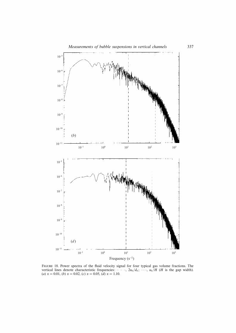
Measurements of bubble suspensions in vertical channels 337
(d )
10–5
10–6
10–7
10–8
10–9
10–10
10–11
10–1 100 101 102 103
Frequency (s–1)
(b)
10–5
10–6
10–7
10–8
10–9
10–10
10–11
10–1 100 101 102 103
Figure 18. Power spectra of the fluid velocity signal for four typical gas volume fractions. Thevertical lines denote characteristic frequencies: – – –, 2ub/db; – · –, ub/H (H is the gap width).(a) α = 0.01, (b) α = 0.02, (c) α = 0.05, (d) α = 1.10.

338 R. Zenit, D. L. Koch and A. S. Sangani
(a) (b)
Figure 19. Image processing. Photographs are converted into binary images. The spacing in thegrid is 1 mm. (a) Original picture, α = 0.02. (b) Binary image, α = 0.02.
1.0
0.8
0.6
0.4
0.2
0 2 4 6 8 10 12 14 16 18 20
Vertical position (mm)
Hor
izon
tal p
ixel
val
ue a
vera
ge
Figure 20. Pixel value averaged over a horizontal line, ψ̄h, is plotted as a function of verticalposition for four different gas volume fractions: · · ·, α = 0.012; – · –, α = 0.027; - - -, α = 0.046;—–, α = 0.116. The horizontal lines show the average pixel value.
of α, it is difficult to detect clusters because the image is almost entirely filled withbubbles.
To test for the existence of horizontally oriented clusters, we considered the varianceof the horizontal mean pixel value Ψh = 〈〈ψ〉2h〉v where 〈 〉h indicates an average overhorizontal and 〈 〉v an average over vertical position. To determine if, in fact, thereexists a preferential horizontal structure in the images, the equivalent expression forpixel variance in the vertical direction can be calculated, Ψv , and compared with theone for the horizontal direction, Ψh. The maximum possible size of a cluster in this

Measurements of bubble suspensions in vertical channels 339
4
3
2
1
0 0.04 0.08 0.12 0.16
Gas volume fraction, α
Rat
io o
f ho
rizo
ntal
to v
erti
cal p
ixel
val
ue v
aria
nce
Figure 21. Ratio of the variances of the horizontally and vertically averaged pixel values Ψh/Ψv , asa function of gas volume fraction. The bars indicate the statistical error in the measurement. Eachdata point results from the processing of six photograph sections.
experiment is of the order of the channel gap width; hence, to better quantify theexistence of clusters averages were performed over 1 × 1 cm2 regions of the images.Figure 21 shows the ratio Ψh/Ψv as a function of the gas volume fraction. Clearly,the figure shows that Ψh is larger than Ψv and the difference is largest for gasvolume fractions in between 0.04 and 0.08. The preferential structure found in thehorizontal direction indicates that clustering is, in fact, occurring. The maximum ofΨh/Ψv around α = 0.05 could result from the fact that the method of analysis is mostcapable of detecting bubble clustering at this intermediate volume fraction for whichthe image is neither nearly all white nor all black.
Note that strong clustering is expected to occur according to the criteria proposed bySpelt & Sangani (1998) for the values of Tb/u
2b measured in this experiment. Although
bubble clustering is indeed observed in the experiment, it is not to the extent observedby Sangani & Didwania (1993) and Smereka (1993). In these studies the suspensionformed horizontal rafts in which bubbles accumulated. Bands of bubbles and clearliquid were observed alternately extending through the entire computational domain.Only qualitative comparisons are possible; however, it is clear that the amount ofclustering found in the experiment is not as strong as that observed in the simulations.In the simulations of Sangani & Didwania and Smereka the bubble velocity variancewas only that produced by non-deformable bubbles with potential flow interactions.The bubble velocity variance measured in our experiments was considerably largerand presumably arose due to bubble–wall interactions, deformability of the bubbles,and/or deviations from potential flow. Spelt & Sangani provide a criterion for stabilityof suspensions with larger velocity variance but they do not quantify the amount of

340 R. Zenit, D. L. Koch and A. S. Sangani
clustering that occurs in unstable suspensions. The more modest clustering seen inour experiments may result from the higher bubble velocity variance, the ability ofthe walls to enhance cluster breakup, or the non-sphericity of the bubbles. Duineveld(1994) observed that oblate bubbles with sufficiently large size and aspect ratio maytend to repel one another in the horizontal direction and this mechanism wouldinhibit cluster formation.
4. Summary and final remarksIn this paper, we have presented the first experimental results concerning the aver-
aged behaviour of bubble suspensions that satisfy the conditions of large Reynoldsnumber and moderately small Weber number necessary for comparison with theoriesbased on potential flow interactions among the bubbles. Nearly monodisperse bubblesuspensions were generated by a bank of identical capillaries. The flow propertieswere measured using two different probes and digital image processing. A hot-wireprobe was used to measure the liquid velocity variance and the bubble–probe collisionrate. The mean and variance of the bubble velocity and bubble–probe collision ratewere measured using a dual impedance probe.
The mean bubble velocity was observed to decrease as the concentration increased,at a rate comparable to that predicted by Spelt & Sangani (1998). The mean bubblevelocity was found to decrease rapidly for very dilute suspensions, resulting from thebubble–wall interactions. The bubble velocity variance increased rapidly with gas vol-ume fraction in very dilute suspensions and more moderately at higher concentrations.
A salient feature of the experiments presented in this paper is the effect of the con-taining walls. The ratio of the channel width to the bubble diameter was moderatelylarge (about 13), so that one might have expected the bulk of the suspension to berelatively unaffected by the walls. However, the walls induce an oscillatory trajectoryon single bubbles moving in the channel in which the bubbles translate to a positionwithin a bubble diameter of one wall and then reverse direction to approach the otherwall.
The bubble velocity variance measured in our experiments was too small to pro-duce a stable suspension according to the criteria proposed by Spelt & Sangani(1998), so we should expect to observe evidence of bubble clustering. Three types ofexperimental evidence for bubble clustering were presented. First, the fluid velocityvariance was found to be about 10 times larger than that which would be produced byhomogeneously distributed bubbles. Second, the power spectrum of the fluid velocityindicated that much of the energy of the fluid motion was at a frequency characteristicof the passage of bubble clusters with a size comparable with the channel diameter.Finally, direct visual evidence was obtained from video images such as that in figure 2and the results of the image processing. The existence of horizontal clusters supportsthe theories for bubbles interacting through potential flow disturbances. The extentof the clustering observed in the experiments is considerably less than that seen inthe simulations.
Although we observed mild bubble clustering in the present experiments, no large-scale instabilities or macroscopic flows were observed. It has been noted by previousresearchers (Lammers & Biesheuvel 1996, for example) that large vortical structuresappear in bubbly columns at sufficiently high gas volume fractions. These strongerinhomogeneities are thought to result from the instability of the suspension to voidfraction waves with vertical wave vectors. The postulated instability mechanisminvolves the dependence of the bubble drag on volume fraction and the inertia
Measurements of bubble suspensions in vertical channels 341
associated with the bubbles’ added mass. Vortical structures moving up and down andextending across the channel width were observed in our apparatus for concentrationslarger than 0.20. Zenit et al. (2000) observed that such instabilities occur at lowerconcentrations for the case of gravity-driven shear flows in inclined channels. Thecriterion for the onset of such instabilities in vertical and inclined channels filled withhigh-Reynolds-number, low-Weber-number bubbles is an interesting topic for futureresearch.
This work was supported by NASA under grant number NAG3-1853. The initialwork on the design of the flow cell and the method of detecting bubble collisionswith hot film probes was performed by Reghan J. Hill and Thulasidas Chelppannair,respectively.
REFERENCES
Biesheuvel, A. & Gorissen, W. C. M. 1990 Void fraction disturbances in a uniform bubbly fluid.Intl J. Multiphase Flow 16, 211–231.
Biesheuvel, A. & Wijngaarden L. van 1982 The motion of pairs of gas bubble in a perfect liquid.J. Engng Maths 16, 349–365.
Bruun, H. H. 1995 Hot-Wire Anemometry, Principles and Signal Analysis. Oxford.
Bulthuis, H. F., Prosperetti, A. & Sangani, A. S. 1995 Particle stress in disperse two-phasepotential flow. J. Fluid Mech. 294, 1–16.
Ceccio, S. L. & Georges, D. L. 1996 A review of electrical impedance techniques for the measuremetof multiphase flows. Trans. ASME: J. Fluids Engng 118, 391–399.
Clift, R., Grace, J. R. & Weber, M. E. 1978 Bubbles, Drops, and Particles. Academic.
Duineveld, P. C. 1994 Bouncing and coalescence of two bubbles in water. PhD thesis, UniversiteitTwente.
Duineveld, P. C. 1995 The rise and shape of bubbles in pure water at high Reynolds number.J. Fluid Mech. 292, 325–332.
Durlofsky, L. & Brady, J. F. 1988 The sedimentation rate of disordered suspensions. Phys. Fluids31, 717–727.
Ishii, M. & Zuber, N. 1979 Drag and relative velocity in bubbly, droplet or particulate flows.AIChE J. 25, 843–855.
Kang, S. A., Sangani, A. S., Tsao, H.-K. & Koch, D. L. 1997 Rhelogy of dense bubble suspensions.Phys. Fluids 9, 1540–1570.
Kok, J. B. W. 1993 Dynamic of a pair of gas bubbles moving through a liquid; Part I: Theory. Eur.J. Mech. B/Fluids 251, 541–560.
Kumaran, V. & Koch, D. L. 1994 The effect of hysrodynamic interactions on the averaged propertiesof a bidisperse suspension of high Reynolds number, low Weber number bubbles. Phys. FluidsA 5, 1135–1140.
Ladd, A. J. C. 1990 Hydrodynamic transport coefficients of random dispersions of hard spheres.J. Chem. Phys 93, 3484–3494.
Lammers, J. H. & Biesheuvel, A. 1996 Concentration waves and the instability of bubbly flows.J. Fluid Mech. 328, 67–93.
Lessard, R. R. & Zieminski, S. A. 1971 Bubble coalescence and gas transfer in electrolitic aqueoussolutions. Ind. Engng Chem. Fundam. 10, 260–269.
Lin, T.-J., Reese, J., Hong, T. & Fan, L.-S. 1996 Quantitative analysis and computations of twodimensional bubble comuns. AIChE J. 42, 301–318.
Liu, T. J. & Bankoff, S. G. 1993 Structure of air-water bubbly flow in a vertical pipe – II. Voidfraction, bubble velocity and bubble size distribution. Intl J. Heat Mass Transfer 36, 1061–1072.
Molerus, O. & Kurtin, M. 1985 Hydrodynamics of bubble columns in the uniform bubblingregime. Chem. Engng Sci. 40, 647–652.
Moore, D. W. 1963 The boundary layer on a spherical gas bubble. J. Fluid Mech. 16, 161–176.
Moore, D. W. 1965 The velocity of rise of distorted gas bubbles in a liquid of small viscosity.J. Fluid Mech. 23, 749–749.

342 R. Zenit, D. L. Koch and A. S. Sangani
Og̃uz, H. N. & Prosperetti, A. 1993 Dynamics of bubble growth and detachment from a needle.J. Fluid Mech. 257, 111–145.
Richardson, J. F. & Zaki, W. N. 1954 Sedimentation and fluidisation: Part I. Trans. Inst. Chem.Engrs 32, 35–53.
Sangani, A. S. & Didwania, A. K. 1993a Disperse phase stress tensor in flows of bubbly liquids atlarge Reynolds numbers. J. Fluid Mech. 248, 27–54.
Sangani, A. S. & Didwania, A. K. 1993b Dynamics simulations of flows of bubbly liquids at largeReynolds numbers. J. Fluid Mech. 250, 307–337.
Smereka, P. 1993 On the motion of bubbles in a periodic box. J. Fluid Mech. 254, 79–112.
Spelt, P. D. M. & Sangani, A. S. 1998 Properties and averaged equations for flows of bubblyliquids. Appl. Sci. Res. 58, 337–386.
Tsao, H.-K. & Koch, D. L. 1994 Collisions of slightly deformable, high Reynolds number bubbleswith short range repulsive forces. Phys. Fluids 6, 671–690.
Tsao, H.-K. & Koch, D. L. 1997 Observations of high Reynolds number bubbles interacting wityha rigid wall. Phys. Fluids 9, 2591–2600.
Valukina, N. V., Koz’menko, B. K. & Kashinskii 1979 Characteristics of a flow of monodispersegas-liquid mixture in a vertical tube. Inzhenerno-Fizicheskii Zhurnal 36, 695–698.
Waniewski, T. A. 1999 Air entrainment by plunging bow waves. PhD Thesis, California Instituteof Technology.
Wijngaarden, L. van 1998 On pseudo turbulence. Theor. Comput. Fluid Dyn. 10, 449–458.
Wijngaarden, L. van & Kapteyn, C. 1990 Concentration waves in dilute bubble/liquid mixtures.J. Fluid Mech. 212, 111–137.
Yurkovetsky, Y. & Brady, J. F. 1994 Statistical mechanics of bubbly liquids. Phys. Fluids 8,881–895.
Zenit, R., Koch, D. L. & Sangani, A. S. 2000 Shear flow of a suspension of bubbles rising in aninclined channel. Under consideration for publication in J. Fluid Mech.
Zhang, D. Z. & Prosperetti, A. 1994 Averaged equations for inviscid disperse two-phase flow.J. Fluid Mech. 267, 185–219.