measurements of volatile organic compounds · pdf filemeasurements of volatile organic...
TRANSCRIPT

MEASUREMENTS OF VOLATILE ORGANIC COMPOUNDS IN DIESEL AND
GASOLINE EXHAUST USING PROTON-TRANSFER REACTION MASS
SPECTROMETRY
By
MYLENE GUENERON
A Thesis submitted in partial fulfillment of therequirements for the degree of
MASTER OF SCIENCE IN ENVIRONMENTAL ENGINEERING
WASHINGTON STATE UNIVERSITYDepartment of Civil and Environmental Engineering
DECEMBER 2012

To the Faculty of Washington State University:
The members of the Committee appointed to examine the
thesis of MYLENE GUENERON, M.S. find it satisfactory and recommend that
it be accepted.
Tom Jobson, PhD., Chair
Tim VanReken, PhD.
Heping Liu, PhD.
ii

Acknowledgments
I would like to thank some people that have been there for me during my master
and helped me go through this great experience.
First of all, I am grateful for Tom Jobson who has been an amazing advisor to
work for. He was available, comprehensive, patient and knows how to stimulate his
students in their work. I would also like to thank the people that I had worked with
in the laboratory: especially Matt Erickson who taught me patiently how to use the
PTR-MS, Graham VanderSchelden who is very easy to work with, Will Wallace who
always had constructive comments on my work, and last but not the least I would
like to particularly aknowledge Claudia Toro who not only helped me go through my
thesis with wise advices but also she was my friend since my �rst day in the program.
I would also like to thank Courtney Herring for her nice collaboration on the LRRI
�eld expreiment.
I also thank my o�ce mates from LAR that gave me great support with a special
mention for Jinshu Chi, also Celia Faiola and Tsenguel Nergui.
I am also thankful for my family and friends who were moral support during my
studies.
Finally I would like to thank the University of Washington Clean Air Research
Center (CCAR), EPA grant #RD83479601, for its funding.
iii

MEASUREMENTS OF VOLATILE ORGANIC COMPOUNDS IN DIESEL AND
GASOLINE EXHAUST USING PROTON-TRANSFER REACTION MASS
SPECTROMETRY
Abstract
by MYLENE GUENERON, M.S.Washington State University
DECEMBER 2012
Chair: Tom Jobson
A Proton Transfer Reaction Mass Spectrometer (PTR-MS) was used to measure the
abundance of organics in diesel and gasoline engine exhaust mixtures as part of a health
effects study conducted at the Lovelace Respiratory Research Institute. To aid in the
interpretation of PTR-MS mass spectra of exhaust mixtures, laboratory experiments
were conducted to better understand the sensitivity and fragmentation patterns for
a series of alkyl substituted monoaromatics and polyaromatic hydrocarbons found in
exhaust. Monoaromatic compound fragmentation was examined for drift tube conditions
of 80, 100, 120, and 150 Td. It was observed that compounds with ethyl or isopropyl
groups attached to a benzene ring are susceptible to fragmentation and can therefore
produce positive inferences in the measurement of benzene and toluene. The sensitivity
of the PTR-MS to the PAH compounds acenaphthylene, acenaphthene, and biphenyl
was determined by preparing standards in dichloromethane and using a syringe pump
to dynamically dilute evaporated standard solutions into a flow of hot dry nitrogen gas.
The sensitivity was found to be 3.1 ±0.3, 3.2 ±0.3, and 3.2 ±0.6 Hz per MHz H3O+
iv

per ppbV respectively at the 80 Td drift tube condition. The PAH compounds did not
fragment and therefore can be monitored at their M+1 ion. The mass spectrums of
diesel and gasoline exhaust were quite similar with a few exceptions. While the gasoline
exhaust had much higher concentrations of volatile organic compounds (VOCs), the
abundance of compounds relative to benzene was similar. Low engine loads had the
highest concentrations for both engines. The data show some evidence that in diesel
and gasoline exhaust mixtures with high particle mass concentrations, PAH compounds
partition from the gas phase to the particle phase and may offer an explanation as to
why gasoline and diesel exhaust mixtures are more toxic than either alone.
v

Contents
Acknowledgments . . . . . . . . . . . . . . . . . . . . . . . . . . . . . . . . iii
Abstract . . . . . . . . . . . . . . . . . . . . . . . . . . . . . . . . . . . . . . iv
List of Tables . . . . . . . . . . . . . . . . . . . . . . . . . . . . . . . . . . . viii
List of Figures . . . . . . . . . . . . . . . . . . . . . . . . . . . . . . . . . . x
1 Introduction . . . . . . . . . . . . . . . . . . . . . . . . . . . . . . . . . . 11.1 Vehicle emissions: e�ect on human health . . . . . . . . . . . . . . . 11.2 Diesel and gasoline composition . . . . . . . . . . . . . . . . . . . . . 31.3 Partitioning hypothesis . . . . . . . . . . . . . . . . . . . . . . . . . . 5
2 Experimental Setup . . . . . . . . . . . . . . . . . . . . . . . . . . . . . 102.1 PTR-MS . . . . . . . . . . . . . . . . . . . . . . . . . . . . . . . . . . 10
2.1.1 PTR-MS measurement principle . . . . . . . . . . . . . . . . . 102.1.2 Intermediate volatile organic compounds (IVOCs) measurements 16
2.2 Dynamic Dilution System . . . . . . . . . . . . . . . . . . . . . . . . 182.2.1 Injection of test mixtures . . . . . . . . . . . . . . . . . . . . . 182.2.2 Calculations of test mixture molar mixing ratios . . . . . . . . 192.2.3 PTR-MS calibration with a compressed gas standard . . . . . 22
3 Experimental Results . . . . . . . . . . . . . . . . . . . . . . . . . . . . 253.1 Dynamic Dilution System . . . . . . . . . . . . . . . . . . . . . . . . 25
3.1.1 Accuracy of the syringe pump infusion rate . . . . . . . . . . . 253.1.2 Aromatic Sensitivities . . . . . . . . . . . . . . . . . . . . . . 263.1.3 Accuracy of the dynamic dilution system . . . . . . . . . . . . 293.1.4 PAH sensitivities . . . . . . . . . . . . . . . . . . . . . . . . . 37
3.2 Fragmentation: dissociative proton transfer reactions . . . . . . . . . 393.2.1 Fragmentation Patterns of Aromatic Compounds . . . . . . . 39
3.2.1.1 Monocyclic aromatic hydrocarbons . . . . . . . . . . 43
vi
3.2.1.2 Naphthalenes . . . . . . . . . . . . . . . . . . . . . . 483.2.1.3 PAHs . . . . . . . . . . . . . . . . . . . . . . . . . . 523.2.1.4 Biphenyl . . . . . . . . . . . . . . . . . . . . . . . . . 52
3.2.2 Fragmentation Pattern Summary . . . . . . . . . . . . . . . . 53
4 LRRI . . . . . . . . . . . . . . . . . . . . . . . . . . . . . . . . . . . . . . 614.1 Purpose of the study . . . . . . . . . . . . . . . . . . . . . . . . . . . 614.2 Exposure chamber experimental set up . . . . . . . . . . . . . . . . . 624.3 PTR-MS Sampling of Chambers . . . . . . . . . . . . . . . . . . . . . 66
4.3.1 Fuels composition and comparison to engine exhaust . . . . . 694.3.2 Comparison of gasoline and diesel exhaust composition . . . . 744.3.3 Particle and engine loading variations . . . . . . . . . . . . . . 75
4.3.3.1 Diesel . . . . . . . . . . . . . . . . . . . . . . . . . . 754.3.3.2 Gasoline . . . . . . . . . . . . . . . . . . . . . . . . . 774.3.3.3 Mixture with variation in the gas and particles loadings 80
5 Conclusions . . . . . . . . . . . . . . . . . . . . . . . . . . . . . . . . . . 83
References . . . . . . . . . . . . . . . . . . . . . . . . . . . . . . . . . . . . . 88
vii

List of Tables
2.1 Mixing Ratios of VOCs in the PTR-MS Calibration Standard tank . 24
3.1 Results on the accuracy of the syringe pump infusion rate . . . . . . . 263.2 Final aromatic sensitivities at Td80 and Td120 . . . . . . . . . . . . . 283.3 Ranges of expected mixing ratio for benzene, toluene, p-xylene and
1,3,5-trimethylbenzene. . . . . . . . . . . . . . . . . . . . . . . . . . . 293.4 PAHs sensitivities at Td80 . . . . . . . . . . . . . . . . . . . . . . . . 383.5 List of compounds tested for fragmentation. . . . . . . . . . . . . . . 413.6 Fragmentation . . . . . . . . . . . . . . . . . . . . . . . . . . . . . . . 60
4.1 Engine load conditions . . . . . . . . . . . . . . . . . . . . . . . . . . 644.2 Experiments Summary . . . . . . . . . . . . . . . . . . . . . . . . . . 654.3 Ions measured with the PTR-MS during the exposure chamber exper-
iment . . . . . . . . . . . . . . . . . . . . . . . . . . . . . . . . . . . . 69
viii

List of Figures
1.1 Illustration of the in�uence of the aerosol mass concentration in thepartitioning process. . . . . . . . . . . . . . . . . . . . . . . . . . . . 6
1.2 Lipid Peroxidal Response to Di�erent Mixing Exposure . . . . . . . . 81.3 Illustration of the repartitioning hypothesis in mixtures of diesel and
gasoline exhausts. . . . . . . . . . . . . . . . . . . . . . . . . . . . . . 9
2.1 Schematic of the PTR-MS . . . . . . . . . . . . . . . . . . . . . . . . 132.2 PTR-MS mass spectrum of a calibration tank experiment at Td80 . . 142.3 Four modes of the cold trap . . . . . . . . . . . . . . . . . . . . . . . 152.4 Schematic of the VOC/IVOC system . . . . . . . . . . . . . . . . . . 172.5 Diagram of the dynamic dilution system setup for making ppbv test
gas mixtures from liquid chemicals. . . . . . . . . . . . . . . . . . . . 202.6 Temperature di�erence in the dynamic dilution system between T1 and
T2 . . . . . . . . . . . . . . . . . . . . . . . . . . . . . . . . . . . . . 202.7 Diagram of the dynamic dilution system setup for calibration tests
using a compressed gas standard. . . . . . . . . . . . . . . . . . . . . 23
3.1 Comparison of the averaged sensitivities between the new tank and oldtank. . . . . . . . . . . . . . . . . . . . . . . . . . . . . . . . . . . . . 27
3.2 1,3,5-trimethylbenzene: measured concentration against expected con-centration for a temperature range of [T=30◦C : T=70◦C] . . . . . . 33
3.3 P-xylene: measured concentration against expected concentration fora temperature range of [T=30◦C : T=70◦C] . . . . . . . . . . . . . . 34
3.4 Toluene: measured concentration against expected concentration for atemperature range of [T=30◦C : T=70◦C] . . . . . . . . . . . . . . . 35
3.5 Benzene: measured concentration against expected concentration fora temperature range of [Troom : T=70◦C] . . . . . . . . . . . . . . . . 36
3.6 Upper limit of vapor pressures . . . . . . . . . . . . . . . . . . . . . . 383.7 Mass spectra of the dichloromethane at Td80 and Td150 . . . . . . . 433.8 Fragmentation of naphthalene: barscan . . . . . . . . . . . . . . . . . 493.9 Fragmentation 1,2-dihydronaphthalene: barscan . . . . . . . . . . . . 51
ix

3.10 Fragmentation acenaphthylene: barscan . . . . . . . . . . . . . . . . . 543.11 Fragmentation acenaphthene: barscan . . . . . . . . . . . . . . . . . . 553.12 Fragmentation biphenyl: barscan . . . . . . . . . . . . . . . . . . . . 563.13 Fragmentation abundance (%) . . . . . . . . . . . . . . . . . . . . . . 573.14 Fragmentation abundance (%)(continued) . . . . . . . . . . . . . . . 583.15 Fragmentation abundance (%)(continued) . . . . . . . . . . . . . . . 59
4.1 General plumbing schematic of the exposure chamber measurements . 634.2 Pictures of the chamber exposure connection with the PTR-MS. . . . 684.3 PTR-MS mass spectra of diesel exhaust and diesel fuel. . . . . . . . . 724.4 PTR-MS mass spectra of gasoline engine exhaust and gasoline fuel. . 734.5 Organics abundance relative to benzene for diesel and gasoline exhaust. 744.6 Impact of diesel particle loading on organics abundance at typical en-
gine loading (total organic abundance). . . . . . . . . . . . . . . . . . 774.7 Impact of diesel particle loading on organics abundance at typical en-
gine loading. . . . . . . . . . . . . . . . . . . . . . . . . . . . . . . . . 784.8 Impact of diesel engine loading on the organic abundance in a diesel
only mixture, at a constant particle loading . . . . . . . . . . . . . . 784.9 Impact of diesel engine loading on the organic abundance in a gasoline
and diesel mixture, at a constant particle loading for both diesel andgasoline . . . . . . . . . . . . . . . . . . . . . . . . . . . . . . . . . . 79
4.10 Impact of particle loading and engine loading variations for gasolineonly mixtures. . . . . . . . . . . . . . . . . . . . . . . . . . . . . . . . 80
4.11 Impact of the increase in the fraction of diesel on the organic abundanceof a mixture (PTR-MS) . . . . . . . . . . . . . . . . . . . . . . . . . 81
4.12 Impact of the increase in the fraction of diesel on the organic abundanceof a mixture (HR-ToF-AMS) . . . . . . . . . . . . . . . . . . . . . . . 82
x

Chapter 1. Introduction
1.1 Vehicle emissions: e�ect on human health
Vehicles emissions are a major source of air pollution in the United States. Ac-
cording to the US Environmental Protection Agency's (EPA) 2008 National Emissions
Inventory, roadway vehicles emissions contribute 17% of the nation's total VOC emis-
sions from anthropogenic sources, 40% of the carbon monoxide (CO) emissions, 38%
of the oxides of nitrogen (NOx) emissions, and 5% of PM2.5 (particulate matter with
a diameter less than 2.5µm) emissions. Since vehicle emissions are concentrated in
urban areas, the relative importance of these emissions to an urban area emission
inventory can be much larger than the national average. Heavy duty diesel vehi-
cles are the most important roadway source of PM2.5 while gasoline vehicles are the
most important source of VOCs and CO. NO2, CO, and PM2.5 are criteria air pollu-
tants and ambient concentrations are regulated by the EPA because of their e�ects
on human health. To reduce exposure to these pollutants vehicle emissions rates of
VOCs, CO, NOx and PM2.5 are also regulated by the EPA. Diesel and gasoline vehicle
exhaust are known to have carcinogenic or respiratory tract irritation e�ects. Diesel
engine PM2.5 emissions are now recognized as being carcinogenic by the World Health
Organization.
1

Pope and Dockery (1), wrote a critical review of several studies on the speci�c ef-
fect of PM on health. While PM2.5 and PM10 mass concentrations are both regulated
by the Environmental Protection Agency with a limitation of 35µg m−3 and 150µg
m−3 for 24 hours respectively, health e�ects may be due to exposure to small submi-
cron sized particles. There are di�erent sizes of particulate matter: coarse particles
with an aerodynamic diameter greater than 2.5 µm, �ne particles with an aerody-
namic diameter less than 2.5µm (PM2.5), and ultra�ne particles with an aerodynamic
diameter less than 0.1µm (PM0.1). The human immune system is complex and very
reactive to cellular intrusion of any unknown substance. When particles enter the cel-
lular layer, the immune system starts up and immune responses can be observed and
quanti�ed. When breathing in gasoline and diesel exhausts a subject inhales these
gases and particles. The particles can deposit inside the respiratory tract. Particles
will settle at di�erent depths inside the respiratory system depending on their size.
Larger particles (larger than 10 µm) get stuck in the upper respiratory tract in the
oral cavity, nasal passage, and trachea. Fine and ultra�ne particles can make their
way deeper to the alveolar region where gas exchange takes place and can even pass
through cell membranes. Particles thus can deliver chemicals to di�erent places in the
respiratory tract and these chemicals are taken up by the body. Mortality increases
with time of exposure to elevated PM concentrations. PM exposure is likely to lead to
cardiovascular mortality, pulmonary in�ammation, subclinical chronic in�ammatory
lung injury, and arterial vasoconstriction (1�10).
2

1.2 Diesel and gasoline composition
There is a special interest in organic compounds from vehicle exhaust as these
compounds are chemically reactive and contribute to ozone and PM2.5 formation in
urban areas (11�13). The organic compounds can be directly emitted in the con-
densed phase as primary organic aerosols (POA) or in the gaseous phase as VOCs
that can further oxidize in the atmosphere to form less volatile compounds called
semi-volatile organic compounds (SVOCs) that can condense onto airborne particles
creating secondary organic aerosols (SOA). In urban areas POAs are mainly emitted
from meat cooking, paved road dust, �replaces and vehicle emissions (14). Many VOC
present in the gas phase have been identi�ed as potential sources of SOA (15�18). To
study vehicles emissions there are two main types of experiments, the dynamometer
studies and the on-road studies that typically make measurements from tra�c tun-
nels. The dynamometer studies provide precise results of emissions factors, but are
not as representative of the actual emissions as the on-road studies. The latter are
more realistic but the test conditions are not well controlled. Standard methods for
hydrocarbon measurement use gas chromatography with either mass spectrometry or
�ame ionization detection. The use of proton transfer reaction mass spectrometry
(PTR-MS) is becoming more wide spread in atmospheric chemistry research. The
GC-MS is useful because it can provide very detailed chemical composition of an air
sample. However, the sample collection process and the subsequent analysis by gas
chromatography requires a considerable length of time so this method cannot be used
for real time monitoring. The PTR-MS was developed in order to monitor pptv (parts
per trillion volume) levels of VOCs in a short period of time without complex sample
3

preparations (19). The PTR-MS provides a less detailed chemical composition of a
sample because it cannot distinguish between compounds of the same nominal mass
but it does have some advantages. One advantage is the PTR-MS measures important
oxygenated compounds such as formaldehyde and acetaldehyde that are di�cult to
sample and measure by gas chromatography. These compounds are directly emitted
in exhaust and are created in photochemical reactions with VOCs in the atmosphere
(20). Both are responsible for health problems (21) and are considered by the EPA as
air toxics. The in-situ, high time resolution measurements of the PTR-MS can also
be advantageous when there is a need to follow rapid changes in concentrations in
ambient air or in laboratory experiments such as the engine exhaust tests described
in Chapter 4.
In studies of urban air pollution, compounds from vehicle exhaust are ubiquitous
and often the most abundant organic compounds in urban air. Urban air can often
look like dilute vehicle exhaust with additional compounds from other sources such as
solvent use and biogenic emissions. Mohamed et al.(22) found that in urban locations
benzene, toluene, and the xylenes and ethylbenzene compounds (aromatics) were the
most abundant organic species and correlated with vehicle emissions. Formaldehyde
and acetaldehyde were also abundant. Organic gaseous compounds emitted in gaso-
line engine exhaust are alkenes, aromatics, and alkanes with 10 or fewer carbon atoms.
The most abundant hydrocarbons are the n-alkanes (n-butane, n-pentane, n-hexane);
the branched alkanes (isopentane, 2-methylpentane, 2,2,4 -trimethylpentane); the un-
saturated compounds (ethene, propene, ethyne); and the monoaromatics (benzene,
toluene, p-xylene and m-xylene) (12, 23�25). Emissions of oxygenated organics such
as formaldehyde and acetaldehyde are also signi�cant (12). The gaseous phase of
4

diesel engine exhaust has not been as extensively characterized as gasoline exhaust
but contains similar compounds to gasoline engine exhaust (23, 24, 26�28). One im-
portant di�erence is the much larger emission rate of formaldehyde and acetaldehyde
from diesel engines, and emission of larger molecular weight compounds (26). The
emission of larger molecular weight compounds re�ects the very di�erent fuel com-
position: gasoline consists of C4 to C10 hydrocarbons, while diesel is composed of C6
to C25 hydrocarbons (25�27, 29). It has been shown that the loading of the engine
also a�ects the composition of the emissions, especially the abundance of alkenes and
alkanes (30).
1.3 Partitioning hypothesis
In exhaust exposure chamber studies of health e�ects, animal subjects are sub-
mitted to a much higher concentration of organic particles than typically found in
ambient air in order to obtain visible e�ects in a short period of time. However, these
methods may a�ect the air chemistry. Organic compounds and semi volatile organic
compounds like polyaromatic hydrocarbons (PAHs) can partition between the gas
phase and the particulate phase. The partitioning of a compound between the gas
and particulate phase is given by equation 1.1 from (18):
CaerCg
= K ×Mtaer (1.1)
where Caer is the aerosol phase concentration (µg m−3), Cg is the gas phase concen-
tration (µg m−3), Mtaer is the total ambient aerosol mass concentration (µg m−3), and
K is the temperature-dependent coe�cient characterizing the partitioning. Thus, the
5

Figure 1.1. Illustration of the in�uence of the aerosol mass concentration in thepartitioning process. An increase in the total aerosol mass concentration leads to thepartitioning of the gas phase compounds into the particulate phase to maintain theequilibrium.
amount of organic compound that would condense into aerosol phase depends on the
amount of organic aerosol present. A higher aerosol mass concentration would allow
more partitioning from the gas phase to the condensed phase as illustrated in Figure
1.1. Exhaust exposure chambers are trying to mimic real world exposures to chemi-
cals, but in scaling the exposure to high concentrations, the organic PM composition
may be signi�cantly di�erent due to scavenging of compounds from the gas phase to
the condensed phase. These particles then carry additional toxic chemical compounds
to the lung.
6

Therefore, the e�ects of exhausts on health that have been observed with such high
concentration chamber experiments may be misleading. The Lovelace Respiratory Re-
search Institute has recently observed that gasoline and diesel exhaust mixtures have
an even larger cardiovascular e�ect in mice than the sum of gasoline exhaust only and
diesel exhaust only. The lipid peroxidal was used as the tracer to determine the health
e�ect. High levels of lipid peroxides are associated with cancer and heart disease. A
synergistic e�ect is observed; the sum of e�ects from pure exhaust is less than the
e�ect for mixtures. Exhaust mixtures are important because this is what people are
exposed to in the real world. As shown in Figure 1.2, a larger response results when
the gasoline and diesel exhausts are mixed than the sum of the gasoline and diesel ex-
haust results separately. The mix of the two exhausts leads to more than three times
the value expected. It is not clear why such a synergistic e�ect would occur. The
working hypothesis illustrated in Figure 1.3 is that under the high particulate load-
ings used in the animal exposure tests (300 µg m−3 or greater) the re-partitioning of
gasoline exhaust compounds from the gas phase onto diesel particulate matter may
increase the toxicity of inhalable particles. To better understand the relevance of
the exposure chambers to real world conditions, measurements of gas phase organ-
ics by PTR-MS and particle phase composition by High Resolution Time-of-Flight
Aerosol Mass Spectrometer (HR-ToF-AMS) were conducted as a multi-investigator
study involving the Jobson and VanReken research groups from the Laboratory for
Atmospheric Research at Washington State University (WSU), investigators from the
School of Public Health at University of Washington, and the inhalation toxicology
group from the Lovelace Respiratory Research Institute (LRRI) in Albuquerque, New
Mexico. This thesis describes laboratory experiments to calibrate the PTR-MS in-
7

strument response to organic compounds expected to be in gasoline and diesel engine
exhaust, and describes results from the exposure chamber characterization studies
conducted at LRRI in the spring of 2012.
Figure 1.2. Lipid Peroxidal Response to Di�erent Mixing Exposure (Source: LRRIresults)
8

Figure 1.3. Illustration of the repartitioning hypothesis in mixtures of diesel andgasoline exhausts.
9

Chapter 2. Experimental Setup
2.1 PTR-MS
2.1.1 PTR-MS measurement principle
The VOC measurements by the PTR-MS are based on a soft ionization of the or-
ganic compounds with the hydronium ion H3O+. The method has been well described
in literature (31), and only the basics of measurement are described in this section.
The instrument is composed of an ion source, a drift tube, a quadrupole mass spec-
trometer and an ion detector as shown in Figure 2.1. The ion source produces a high
density of hydronium ions from water vapor using a hallow cathode discharge. O+2
and NO+ can also be produced but are considered as impurities. Those primary ions
are transported into the drift tube reactor where the sample air is also introduced.
The H3O+ ion does not react with gaseous components that have a proton a�nity
less than water vapor (697±8 kJ mol−1). As the major components of air have low
proton a�nity it acts like a bu�er gas, and the organic compounds (R) with large
enough proton a�nities that are present in the sampled air undergo a non dissociative
proton transfer reaction as described in equation 2.1:
H3O+ +R RH+ +H2O (2.1)
10

where R is the organic compound present in the sample, H3O+ is the hydronium ion
produced in the ion source and RH+ is the product ion. O+2 and NO+ can react with
organic compounds which would interfere with the results so their concentrations in
the drift tube are kept under 2% and 0.2% of H3O+ respectively. The drift tube is
made of stainless steel rings separated by Te�on rings to isolate them electrically and
connected by a resistor chain to create an electric �eld. This electric �eld enhances
the kinetic energy of the ions so that collisions with the bath gas (air) cause de-
solvation of hydrated ions. The water vapor present in the drift tube can bind with
the reagent ions H3O+ and the product ions RH+ to form water clusters H3O
+(H2O)
n
and RH+(H2O)
nwhere n is an integer. An interesting reaction that is of importance
when sampling high VOC concentrations is that the RH+(H2O) water clusters can
then react with H2O and reform the R as described in following reactions 2.2, 2.3
called the Ligand switching reaction:
RH+ +H2O RH+(H2O) (2.2)
RH+(H2O) + H2O H+(H2O)2 +R (2.3)
The extent of water cluster formation is a strong function of the drift tube pressure
and electric �eld. To prevent the clustering and thus simplify the mass spectrum, the
reaction chemistry is performed in a drift tube so the clusters concentrations are
reduced to a minimum by collision induced dissociation with air molecules in the
drift tube. Drift tube reaction dynamics are characterized by the ratio of the electric
�eld E (volts per centimeter) over the number density of gas N (cm−3) in the drift
11

tube according to equation 2.4. The units of this ratio are expressed in Townsend
(Td) where 1 Td is equal to 10−17 (V cm−2).
Drift �eld strength =E
N(V cm−2) (2.4)
The number density of air in the drift tube is temperature and pressure dependent.
An increase in the electric �eld (higher Td) results in more energetic collisions and
less clustering but also leads to a greater degree of dissociative protonation and the
creation of organic fragment ions. Such fragmentation is not desirable since the
interpretation of the PTR-MS mass spectrum relies upon its presentation as a simple
M+1 mass spectrum where M is the molecular weight of R. The instrument is usually
run at 120-150 Td with the drift tube pressure at 2 mbar. Ions are sampled from
the drift tube by electrostatic lenses and are mass �ltered by a quadrupole mass
spectrometer. Ions are detected and counted with a secondary electron multiplier
detector (SEM). The H3O+ ion count rate is typically 5 MHz and is much higher
than the concentration of the product ions RH+ so that the concentration of R can
be calculated as given in equation 2.5:
[Ri] =[RH+]
ki · t · [H3O+]
×ε[RH+]
ε[H3O+]
(2.5)
where [Ri] is the number density of the organic compound i, [RH+] is the measured
count rate of the product ion (Hz), [H3O+] is the measured count rate of the reagent
ion (Hz), t is the reaction time that corresponds to the time H3O+ spent in the
drift tube (about 0.1ms), ki is the H3O+ reaction rate constant with compound i,
and ε[RH+] and ε[H3O+] are the ion transmission e�ciencies through the quadrupole
12

water vapor
H+H2O+OH+H2+
Drift Tube reactor
Turbo molecular pumps
Mass spectrometer
detector
low pressure = 0.1 mbarPdrift = 2 mbar
sample inlet
drift electric field = 66 v/cm
Distance = d = 9.2 cm
Ion Source
hollow cathodequadrupole
V drift
stainless steel ring
H3O+
H2O (H2O+) + (R) --> (RH+) + (H2O)
P= 10-5 mbar
Figure 2.1. Schematic of the PTR-MS
for RH+ and H3O+ respectively. The PTR-MS measurements result in mass spectra
(m/z) of the protonated compounds (molecular weight of MW+1 that were detected
by the quadrupole. The mass spectrometer is operated in either a scan mode whereby
all ions over some m/z range are consecutively measured or in MID mode whereby
only selected ions are measured. An example of a mass spectrum obtained from a
calibration tank experiment is shown in Figure 2.2.
The VOC analysis can be improved by using a water trap that removes the water
vapor from a sample to reduce clustering and allows the drift tube to be operated
at lower Townsend numbers (32). The advantage of operating the PTR-MS at lower
13

Figure2.2.PTR-M
Smassspectrum
ofacalibration
tankexperim
entat
Td80
14

- 30C + 65 C
Sample
Dry nitrogenMeasurement
Measurement
Sample Sample
- 30C - 30C
I: Tube 2 back flush mode
1 2
1 2
II: Tube 2 conditioning mode
- 30C+ 65 C
Dry nitrogen
Measurement
Sample Sample
- 30C - 30C
III: Tube 1 back flush mode
2
1 2
IV: Tube 1 conditioning mode
Sample
Measurement
1
exhaust air - out exhaust air - out
exhaust air - out exhaust air - out
Figure 2.3. Four modes of the cold trap. The tubes are measuring one after the other.For each tube there are three periods of time: a back �ush period to eliminate anycompounds from the previous measurement with a temperature of 65◦C, a conditioningperiod characterized by a cold temperature of -30◦C, and a measurement period whenthe PTR-MS samples air �owing through the tube.
Td values, such as 80Td, is increased sensitivity, reduced fragmentation, and a vaste
improvement in the measurement of formaldehyde which displays a water vapor de-
pendent sensitivity. The cold trap is composed of two tubes that are run in four
modes as describes in Figure 2.3. The PTR-MS used in this work is operated with
a water trap. To measure volatile organic compounds the sample is dried by passing
the air through a cold trap held at -30◦C. Furthermore, a second inlet has been added
to improve detection limits of higher molecular weight compounds that are present
at low concentrations.
15
2.1.2 Intermediate volatile organic compounds (IVOCs) measurements
The IVOC species are present at lower concentrations, so are di�cult to mea-
sure directly by PTR-MS. The thermal desorption system that has been developed
accumulates the sampled air on a Tenax TA adsorbent resin to obtain higher concen-
trations of IVOCs that are measurable by the PTR-MS. Sampling through the Tenax
eliminates the compounds with higher volatility from the sample air so that it is pos-
sible to distinguish between volatile compounds and higher molecular weight organics
by using the combination of the water trap and the thermal desorption system. The
VOC and the IVOC inlets are separate but instrument operation allows for switching
from one inlet to the other as shown in Figure 2.4. The IVOC system runs by cycles
of four consecutive modes: sample mode, purge mode, measure mode and back �ush
mode. Each is characterized by a speci�c Tenax trap temperature and a time period.
The measurements of VOCs are implemented while the sample is being collected on
the Tenax trap. The sample mode corresponds to the collection of the sample on the
Tenax tube for usually 180 seconds at 30◦C. The compounds with lower volatility are
more e�ciently adsorbed than those with high volatility. The purge mode consists in
�owing dry nitrogen through the Tenax to �ush out the lighter compounds. A longer
purge time at a higher temperature would remove more compounds. The typical
purge time period is about 120 seconds at 150◦C. During the measure mode the air
�ow is pushed through the Tenax in the opposite direction to the drift tube. For the
IVOC measurements time is limited, therefore we need to choose the speci�c masses
that we want to work on before running the experiment, to have enough time and
obtain a good data set. Usually the measurement period lasts for 300 seconds at a
230◦C. The fourth mode, back �ush, is used to clean up the Tenax. The temperature
16

Figure 2.4. Schematic of the VOC/IVOC system
and the time period are usually 230◦C for 180 seconds, and the air �ow is directed
the opposite way as the measure mode to remove compounds still in the trap so it is
clean for the next cycle.
17

2.2 Dynamic Dilution System
A dynamic dilution system based on a syringe pump to dispense accurate molar
�ows of liquid chemical compounds was used to prepare test mixtures for analysis by
PTR-MS. A recent study from C.L. Faiola et al. (33) showed good results from this
system that was used to generate standard mixtures of trace VOCs. Here, the dynamic
dilution system was used to make test mixtures of compounds that are not stable as
compressed gas mixtures. These test mixtures were used to examine fragmentation
patterns and to determine the sensitivity of the PTR-MS to PAH compounds. The
accuracy of the dynamic dilution systems was evaluated by comparing test mixtures
prepared from neat liquids against the compressed gas VOC standard typically used
to calibrate the PTR-MS. The experimental set-up of the dynamic dilution system
was similar for both types of tests with a few exceptions as described below.
2.2.1 Injection of test mixtures
The dynamic dilution system is divided into three parts for ease of description: the
dry nitrogen dilution �ow, the syringe pump, and the test mixture �ow. The set-up of
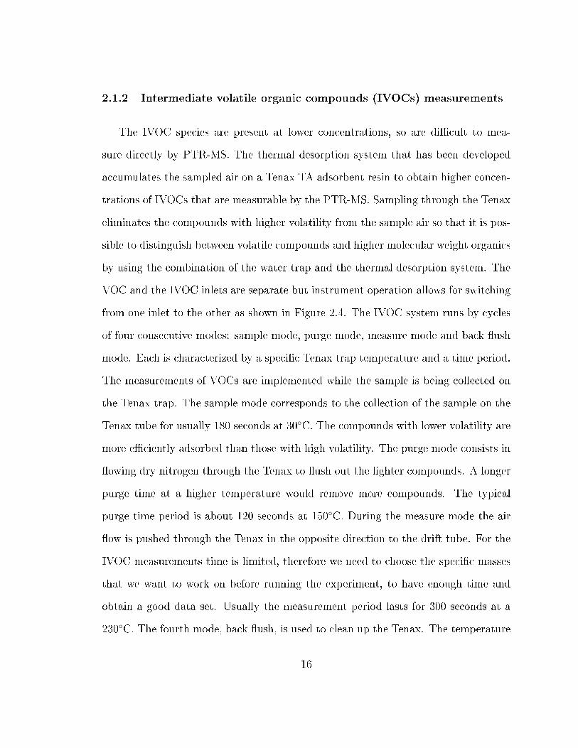
the dilution system is sketched in Figure 2.5. A known molar �ow rate of a compound
is injected using the syringe pump into a heated zone where it evaporates from the
syringe tip and is diluted by a dry nitrogen �ow supplied from a liquid nitrogen
dewar. The PTR-MS subsampled from the test mixture �ow and the rest of the �ow
was vented to the laboratory fumehood. The dry nitrogen �ow was controlled by a
MKS mass �ow controller to provide a known dilution �ow. The syringe pump used
was a Harvard Apparatus PHD 2000 infusion pump. The syringe type used in the
18

experiments was the Hamilton Gastight in a size range of 0.1 to 50 µl. The tubing
and �ttings for the system were stainless steel or Restek Sul�nert coated stainless
steel tubing. To keep the injected compounds in the gas phase and avoid potential
wall losses, the tubing and �ttings were heated using heat tape. The temperature
of the injection zone (T1) was thermostated using a temperature controller (Watlow)
with a type K thermocouple wire measuring the air�ow temperature at point T1
as shown in the Figure 2.5. Typical injection temperatures were between 30 and
70◦C. A second thermocouple measured the temperatures immediately downstream
of the injection zone (T2). The stainless steel tubing downstream from the injection
zone was coiled to enhance mixing. This tubing was wrapped in heat tape and the
temperature controlled by a variac. Downstream tubing temperature was estimated
to range between 80 and 90◦C. This temperature may have in�uenced the actual
temperature of the injection by heat conducted through the hot tubing. A di�erence
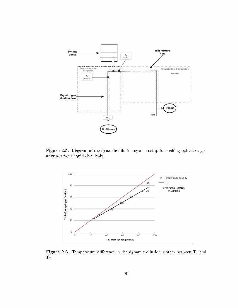
in temperature between T1 and T2 was observed as shown in Figure 2.6. At T1 set
point temperatures of between 30 and 40◦C, the di�erence between T1 and T2 is small,
on the order of a few degrees. At a set-point temperature of 50◦C, the downstream
temperature at T2 was about 10◦C warmer. At a T1 temperature of 70◦C and greater
the T2 temperature was consistently about 90◦C, and re�ects the temperature of the
downstream tubing temperature.
2.2.2 Calculations of test mixture molar mixing ratios
The molar mixing ratio of the prepared test mixture (Xi) can be calculated from
the molar �ow of the injected liquid (MFi) and the molar �ow of the diluting gas
(MFN2) as given in equation 2.6 .
19
Syringepump
Dry nitrogendilution flow
Dry Nitrogen
MFC
PTR-MS
vent
Variac Controlled Temperature
[80 -90] C
Test mixtureflow
Temperature zoneof injection
T1[30 - 70] C
T2[40 - 90] C
Figure 2.5. Diagram of the dynamic dilution system setup for making ppbv test gasmixtures from liquid chemicals.
y = 0.7946x + 3.9316 R² = 0.9543
0
20
40
60
80
100
0 20 40 60 80 100
T1: b
efo
re s
yrin
ge (
Ce
lsiu
s )
T2 : after syringe (Celsius)
Temperature T1 vs T2
1:1
Figure 2.6. Temperature di�erence in the dynamic dilution system between T1 andT2
20

Xi = 109 × MFi
MFN2
(ppbv) (2.6)
Those two molecular �ows can be determined as shown in equation 2.7,
Xi = 109 ×Ir × µi
1000×MWi
60× GFN2
VmN2
(ppbv) (2.7)
where Ir is the infusion rate of the syringe pump in µl hr−1, µi is the density of
the compound i in g mL−1, MWi is the molecular weight of the compound i in g
mol−1, GFN2 is the gas �ow of the dry nitrogen in slpm, and VmN2is the molar
volume of gas at standard temperature and pressure. The standard temperature and
pressure reference conditions used by the MKS mass �ow controller are 1 atmosphere
and 273 K, resulting in a molar volume of 22.42 L mol−1. Some of the compounds
examined (acenaphthene, biphenyl and acenaphthylene) were in the solid phase at
room temperature. For a solid compound j, it was necessary to �rst dissolve it in
a solvent. Cj is the concentration resulting from that dissolution. Dichloromethane
was chosen as a solvent for the dissolution because it has a proton a�nity lower than
H2O and therefore can't be detected by the PTR-MS. The molar �ow of the solid
compound j injected by the syringe pump does not depend on the density anymore
but on the solution concentration Cj. The test mixture molar mixing ratio is given
by 2.8:
Xj = 109 ×Ir × Cj
1000×MWj
60× GFN2
VmN2
(ppbv) (2.8)
where Cj is the concentration of the compound j in g mL−1. Solutions were made up
21

using 10 mL and 100 mL volumetric �asks. The solid compounds were weighed using
an analytical balance (Mettler H2O WWR scienti�c) that allows a precision to 10−5
g. The �nal Cj was about 0.002 g mol−1.
2.2.3 PTR-MS calibration with a compressed gas standard
To determine the accuracy of the dynamic dilution system the setup is slightly
di�erent because we are mixing two gas �ows, the one from the compressed gas multi-
component calibration tank and the other from the dilution �ow of dry nitrogen. The
set up for the calibration study is described in Figure 2.7. The set up is divided into
three parts again for ease of description: the dry nitrogen dilution �ow, the calibration
tank �ow, and the test mixture �ow connected to the PTR-MS inlet. The calibration
for the PTR-MS is performed using a special tank composed of known concentrations
of speci�c VOCs. The tank used in our laboratory is from Scott Marrin, Inc, and its
whole composition is detailed in Table 2.1. The accuracy of the standard is ± 10% as
stated by the manufacturer. The sensitivities of the PTR-MS for those compounds
can be calculated using equation 2.9 :
Si =NC
Xi
(Hz per MHzH3O+ per ppbV) (2.9)
Xi =Ci × FcFd + Fc
(ppbv) (2.10)
where Si is the sensitivity of the compound i, NC is the normalized count from
the PTR-MS measurement (Hz per MHzH3O+ per ppbV), Xi the compounds molar
mixing ratio in ppbv calculated from equation 2.10, Ci is the mixing ratio of compound
22

i in the calibration tank in ppbv, Fc is the �ow from the calibration tank in sccm
(typically 10 sccm), and Fd is the dilution �ow of dry nitrogen in sccm (typically 1016
sccm).
Dry Nitrogen
MFC
Calibration tankCompressed gas
MFC
Calibrationtank flow
PTR-MS
vent
Dry nitrogendilution flow
Test mixtureflow
10 sccm 1016 sccm
Figure 2.7. Diagram of the dynamic dilution system setup for calibration tests usinga compressed gas standard.
23

Table
2.1.MixingRatiosof
VOCsin
thePTR-M
SCalibration
Standardtank
No.
Compound
MW
(g.mol−
1)
m/z
Mixingratio(ppmv)
1methanol
3233
22
acetonitrile
4142
23
acetaldehyde
4445
24
acetone
5859
25
isoprene
6869
26
methacrolein
7071
27
2-butanone
(MEK)
7273
28
benzene
7879
29
toluene
9293
210
styrene
104
105
211
p-xylene
106
107
212
1,2,4-trimethylbenzene
120
121
213
a-pinene
136
137
214
1,2,3,5-tetram
ethylbenzene
134
135
0.5
24

Chapter 3. Experimental Results
3.1 Dynamic Dilution System
3.1.1 Accuracy of the syringe pump infusion rate
The volume of the compounds injected into the dynamic dilution system is in the
order of µL, thus the accuracy of the syringe pump was veri�ed. Two syringes S1
and S2 of 50 µL were �lled with p-xylene and weighed using the analytical balance
before and after injection. The expected volume loss was calculated from the infusion
rate and the time of infusion as shown in equation 3.1. The expected mass loss was
calculated with the density of p-xylene as shown in equation 3.2 :
Expected volume loss = IR × T (3.1)
where IR is the infusion rate in µl hr−1 and T is the time of infusion in hr.
Expected mass loss = Expected volume loss× µ (3.2)
where µ is the density of p-xylene 8.61 10−4 g µl−1
Four tests were performed and the results are summarized in Table 3.1. The average
25

volume error between the expected and actual loss was 0.5% ±1. The small mass loss
was more di�cult to measure and the results present larger average mass error loss
of -0.7% ±8.3. The negative value is representative of a smaller measured mass loss
than the expected one. According to those results, the syringe pump is considered
accurate for further analysis.
Table 3.1. Results on the accuracy of the syringe pump infusion rate
units test 1 (S1) test 2 (S2) test 3 (S2) test 4 (S2)
volume initial ul 50 50 50 50volume �nal ul 0 37.5 37.5 41.5volume loss ul 50 12.5 12.5 8.5
mass initial g 24.536 24.349 24.343 24.342mass �nal g 24.495 24.339 24.331 24.335mass loss g 0.041 0.010 0.012 0.007
Infusion rate ul hr 50 50 50 50time hr 1 0.25 0.25 0.1667
expected volume loss ul 50.0 12.5 12.5 8.3expected mass loss g 0.043 0.011 0.011 0.007
volume di�erence % 0% 0% 0% 2%mass di�erence % -5% -7% 11% -2%
3.1.2 Aromatic Sensitivities
Sensitivity tests for compounds present in the compressed gas calibration tank
have been performed and their �nal average sensitivities at Td=80 and Td=120 are
given in Table 3.2. The calibration tank �ow remained open for at least 3 hours
and sometimes overnight (but less than 24 hours) to condition all tubing before mea-
surements were made. The concentration of the compounds present in the calibration
26

Figure 3.1. Comparison of the averaged sensitivities between the new tank and oldtank.
tanks were con�rmed by analysis on a GC-MS system. Two identical VOC calibration
tanks from Scott Marrin were compared, one older and nearly depleted and the other
newer. Results in Figure 3.1 shows the resulting normalyzed sensitivities and these
were generally within the 10% expected accuracy. The old tank sensitivity values
are slightly higher. To determine the importance of conditioning another experiment
was performed whereby the cal gas �owed for 5 days instead of less than 24h. The
sensitivities were higher and the results are shown in Table 3.2. According to those
tests the sensitivity values are in�uenced by the conditioning time, requiring more
than 24 hours.
27

Table
3.2.Final
arom
aticsensitivities(N
CPS)at
Td80
andTd120foraconditioningtimeof
less
than
24handmore
than
5days.
Percentdi�erence
forthetwoconditioningtimeresults.
conditioningtime:
conditioningtime:
%di�erence
≤24h
≥5days
m/z
Sensitivity
Sensitivity
m/z
Sensitivity
Sensitivity
Td80
Td120
Td80
Td120
3315.9
±1.6
9.6±
1.0
3321.2
10.4
25%
4224.2
±3.7
14.3
±1.3
4234.7
19.3
30%
4518.2
±2.8
11.2
±1.4
4549.6
18.2
63%
5918.1
±3.0
10.8
±1.5
5926.7
14.8
32%
699.9±
1.9
5.3±
1.0
6914.5
6.9
32%
717.7±
2.0
4.3±
1.0
7111.4
5.0
32%
7318.7
±3.7
10.8
±2.0
7327.4
15.3
32%
797.9±
1.5
5.1±
1.0
7912.1
7.9
35%
813.2±
0.5
2.5±
0.5
814.9
4.0
35%
937.5±
1.2
4.7±
0.9
9311.0
6.9
31%
105
6.7±
1.4
4.1±
1.0
105
9.9
6.3
32%
107
6.3±
1.1
3.8±
0.8
107
9.0
5.6
30%
121
4.8±
1.2
3.0±
0.8
121
6.8
4.1
29%
135
4.8±
1.7
2.1±
1.3
135
7.3
4.3
35%
137
2.4±
0.4
1.1±
0.2
137
3.1
1.5
22%
28

3.1.3 Accuracy of the dynamic dilution system
Mixtures of 4 compounds, benzene, toluene, p-xylene and 1,3,5-trimethylbenzene
were prepared to test the accuracy of the dynamic dilution system. Those compounds
were present in the Scott Marrin calibration standard and their sensitivities were
already determined (see Table 3.2). The tests were usually run at 5 injection manifold
temperatures: T1=30◦C, T1=40◦C, T1=50◦C, T1=60◦C, T1=70◦C . Benzene was also
run at room temperature. The infusion rates were varied between 0.1 µl hr−1, 0.25
µl hr−1, 0.5 µl hr−1, and 5 µl hr−1 with a nitrogen �ow of 15 slpm or 20 slpm. At
0.1 µl hr−1 no test for benzene and pxylene were run. The ranges of the expected
concentrations for the 4 compounds are given in Table 3.3. The tests were divided
into two sets: low mixing ratio tests that correspond to mixing ratios ≤ 200 ppbv
and high mixing ratio tests that correspond to mixing ratios ≥ 800 ppbv.
Table 3.3. Ranges of expected mixing ratio for benzene, toluene, p-xylene and 1,3,5-trimethylbenzene.
Compounds Mixing ratio range (ppbv)low mixing ratios high mixing ratio
Infusion rate (ul/hr) 0.1 0.25 0.5 0.1 5N2 Flow (slpm) 15 15 15 20 20
benzene 28 70 140 . 1350toluene 23 58 116 17 1126pxylene 20 50 109 . 973
1,3,5-trimethylbenze 18 45 91 14 875
The 1,3,5-trimethylbenzene is the less volatile compound tested with the lower
vapor pressure. This compound displays a good correlation between the expected
and measured mixing ratios as shown in Figure 3.2. The measured mixing ratios are
29

within the 20% of the expected mixing ratios. At smaller infusion rates the measured
mixing ratio is higher than expected, and for the expected 875 ppbv test mixture
the measured mixing ratio is smaller by less than 10%. The T=40◦C results for low
mixing ratios and the two data points for T=50◦C come from the same experiment
that is considered as an outlier for the analysis because the points do not follow the
trend of all the other points. The error bars correspond to the standard deviation of
multiple tests.
The p-xylene also displays a good correlation between the expected and measured
mixing ratios as shown in Figure 3.3. The measured mixing ratios are smaller than
expected by less than 20% for mixing ratios less than 120 ppbv at T=30◦C to T=70◦C.
For the expected mixing ratio of 973 ppbv, at T=30◦C, 40◦C and 50◦C the measured
and expected mixing ratio match; at T=60◦C and T=70◦C the measured mixing
ratios are larger by less than 10% and 20% respectively. The T=40◦C results for
low mixing ratios and the two data points for T=50◦C are considered as outliers in
this analysis as it comes from the same experiment previously described as an outlier
for 1,3,5-trimethylbenzene. The error bars correspond to the standard deviation of
multiple tests.
The results for toluene are shown in Figure 3.4. The measured concentration at
T=40◦C is within 20% of the expected concentration and within 30% of the highest
infusion rate that produced a 1126 ppbv test mixture. At T=50◦C there is good
agreement between the expected and measured mixing ratios, within 20% for mixing
ratios less than 60 ppbv. At T=60◦C, the results show that the measured mixing
ratio is always higher than expected, at 18 ppbv expected the measured mixing ratio
is less than 20% higher, but for the other expected concentration the measured mixing
30

ratios are more than 20% higher. At T=70◦C the measured mixing ratios are higher
than expected for both low (18 ppbv) and high (1126 ppbv) mixing ratios. At the
116 ppbv expected there is a point that shows a measured mixing ratio lower by more
than 20% at T=50◦C and a point in the 20% di�erence range at T=60◦C. Those two
points result from the same experiment set and do not follow the trend of the other
points perhaps due to incorrectly recorded �ows, so both are considered as outliers.
For a mixing ratio less than 120 ppbv the ideal temperature to run toluene is around
T=40◦C, measured mixing ratios are lower than expected by more or less 20%. At
small mixing ratios (low infusion rates) and low temperature the excessive evaporation
appears to be an in�uence for toluene. At T=60◦C and T=70◦C the infusion rate
may too low given the toluene vapor pressure at these temperatures and excessive
evaporation from the syringe may be producing higher count rates that expected.
Benzene is the most volatile compound tested with the higher vapor pressure.
All the mixing ratios measured are higher than expected for the whole temperature
range as shown in Figure 3.5. For an expected mixing ratio of 28 ppbv, at Troom
the measured mixing ratio is 10% larger. For an expected mixing ratio of 70 ppbv,
the measured mixing ratio was larger by more than 20% at Troom, more than 30% at
T=40◦C and more than 40% at T=50◦C. For an expected mixing ratio of 140 ppbv,
the measured mixing ratio at Troom, T=40◦C and T=50 ◦C are all larger by more
than 30%. For the expected mixing ratio of 1340 ppbv, the measured concentration
are less than 10% larger at T=30 ◦C and T=40◦C, less than 20% larger at T=50◦C
and T=60◦C, and 30% larger at T=70◦C. The small expected concentrations were
obtained with an infusion rate of 0.1 µl hr−1, 0.25 µl hr−1, and 0.5 µl hr−1, and the
high expected concentration was obtain for an infusion rate of 50 µl hr−1. The results
31

show that only at higher infusion rates is the measured concentration close to what is
expected, and the di�erence increases as the infusion manifold temperature increases.
The discrepancy is likely due to benzene vapor di�using from the syringe tip at a
rate that is greater than the infusion rate. At higher infusion manifold temperatures
and low infusion rates, this evaporative loss might be causing a greater mass loss
of benzene than is calculated from the infusion rate and lead to higher measured
mixing ratios. The usefulness of the dynamic dilution system may be limited to lower
volatility compounds and higher infusion rates.
The test conditions are summarized in Figure 3.6. The �gures show the vapor
pressures of the aromatics tested versus temperature. The plain circles around data
points indicate tests where the measured mixing ratio was within 20% of the expected
mixing ratio. The data points with dashed circles indicate tests conditions where the
measured mixing ratio was more than 20% greater than expected. In general, we
can conclude that for infusion rates less than 0.5 µl hr−1 the best results (agreement
within 20%) were obtained when compound vapor pressures were less than 100 Torr.
For infusion rates of 50 µl hr−1, manifold temperature leading to vapor pressures
up to 300 Torr could be used. For best operation of the dynamic dilution system
it makes sense that the injection manifold temperature be adjusted to account for
the compounds volatility. Operating at too high a temperature may cause excessive
evaporation from the syringe and a mass loss that is greater than the infusion rate.
If the injection manifold temperature is too low it was observed that an erratic PTR-
MS signal would result suggesting droplet formation and loss from the syringe tip.
The dynamic dilution system was put together to determine the sensitivities of the
compounds like PAHs that are important for the charecterization of the exhausts but
32

Figure3.2.1,3,5-trim
ethylbenzene:
measuredconcentrationagainst
expectedconcentrationforatemperature
range
of[T=30
◦ C:T=70
◦ C]
33

Figure3.3.P-xylene:
measuredconcentrationagainst
expectedconcentrationforatemperature
range
of[T=30
◦ C:
T=70
◦ C]
34

Figure3.4.Toluene:
measuredconcentrationagainst
expectedconcentrationforatemperature
range
of[T=30
◦ C:
T=70
◦ C]
35

Figure3.5.
Benzene:
measuredconcentrationagainst
expectedconcentrationforatemperature
range
of[Troom
:T=70
◦ C]
36

do not exist in calibration tanks. The good accuracy of the dynamic dilution system
for the lower vapor pressure compounds, p-xylene and trimethylbenzene, permits to
assume that for mixtures of PAHs introduced in the system the measured mixing ratio
corresponds to the expected mixing ratio providing the required value to calculate
their sensitivities.
3.1.4 PAH sensitivities
The sensitivities for acenaphthene, acenaphthylene and biphenyl were tested using
the dynamic dilution system heated up to 85◦C to avoid wall deposition of those heavy
compounds. These compounds are solid at atmospheric conditions so a solution with
diclhoromethane was made (100 mg into 200 mL). The N2 dilution �ow varied between
1.1 slpm and 5.1 slpm, and the injection rate varied between 20 µl hr−1 and 50 µl
hr−1 to obtain di�erent ranges of concentration. As the accuracy of the dynamic
dilution system has been prooved, especially for lower vapor pressure compounds, it is
assumed that the expected concentration corresponds to the measured concentration.
The sensitivities Si obtained is the fraction of the measured normalized counts NC (in
Hz per MHz H3O+) over the expected concentration in ppbv. The resulting average
sensitivities are summarized in Table 3.4.
37

Figure 3.6. Upper limit of vapor pressures for: benzene, toluene, p-xylene and 1,3,5-trimethylbenzene. Top: Infusion rate less than 0.5 µl hr−1. Bottom: Infusion rate of 5µl hr−1.
Table 3.4. PAHs sensitivities at Td80
compounds (MW+1) sensitivities (NCPS) stdv
Acenaphthylene (153) 3.1 0.3Acenaphthene (155) 3.2 0.3
Biphenyl (155) 3.2 0.6
38

3.2 Fragmentation: dissociative proton transfer reactions
3.2.1 Fragmentation Patterns of Aromatic Compounds
Dissociative proton transfer reactions can occur in the drift tube of the PTR-MS
causing the formation of lower mass fragment ions. It is known that the degree of
dissociation that occurs is a function of the E/N value; higher Townsend operation
implies larger H3O+ kinetic energy. The collision energy of the reaction and resulting
collisions of the RH+ product ion with the bath gas can cause dissociation. The ge-
ometry and functional groups attached to the compound are important parameters
in determining the extent of fragmentation and the likelihood that a compound can
be detected at the RH+ product ion mass. The fragmentation of alcohols, aldehy-
des, ketones and esters compounds has been well documented in the literature (34).
While fragmentation of light aromatic compounds is known, little is known about the
fragmentation of larger alkyl substituted aromatic compounds found in diesel engine
exhaust. The dissociation products may distort the measurements of a sample com-
position, overvaluing the concentration of the products resulting from fragmentation
and underestimating the concentration of the actual compounds present in the sam-
ple. A clear understanding of the dissociation reactions is important for interpreting
the accuracy of PTR-MS measurements, especially for complex mixtures found in
exhausts and ambient air. For our study, some aromatic compounds that are present
in gasoline and diesel engine exhausts, from a molecular weight of 120 g mol−1 to 154
g mol−1 with di�erent molecular structures, were selected and injected separately in
the PTR-MS at Townsend numbers of 80, 100, 120 and 150. The aim of these ex-
periments was to understand which types of species are likely to fragment into which
39

products, and to quantify their fragmentation patterns. The studied compounds and
their molecular structures are listed in Table 3.5 and ordered by molecular weight.
The purity of the compounds ranged from 89% to 99.5%. Also, some of the com-
pounds are solids at room temperature conditions of the laboratory so were dissolved
in dichloromethane. The composition and the dilution ratio of the compounds studied
for fragmentation are summarized in Table 3.5. To organize the results the aromatic
compounds have been classi�ed into the four following families: monocyclic aromatic
hydrocarbons, PAHs, naphthalene and structurally related compounds, and biphenyl.
The monocyclic aromatic hydrocarbons group corresponds to a single benzene
ring (6 carbon atoms) with an alkyl group attached to it. It is known that some
of these compounds fragment. For example ethylbenzene, a common constituent
in urban air, partially fragments to produce an ion at m/z=79 and m/z=107 (32).
Fragmentation of ethylbenzene causes a positive interference for measuring benzene
at m/z=79. Our hypothesis is that monocyclic aromatics with ethyl, propyl, or butyl
groups attached to the ring may be prone to dissociation. Fragmentation of high
molecular weight monocyclic aromatics found in diesel fuel and exhaust may produce
interfering fragment ions for both benzene and toluene (m/z=93). Also of interest is
whether fragmentation of alkyl substituted monocylic aromatics would produce ions
at the series m/z=43, 57, 71, 85, 99. These ions could potentially be used to measure
the abundance of alkanes (35) and thus would produce a positive interference. In
contrast to the monocyclic aromatics, the poly aromatic compounds are not thought
to fragment though this has not been reported in the PTR-MS relevant literature.
Using electron impact ionization fragmentation patterns as a guide, these compounds
typically show a strong molecular ion and do not extensively fragment. The biphenyl
40

Table 3.5. List of compounds tested for fragmentation.
41

group structures are based on two benzene rings connected by a carbon-carbon single
bond. Alkyl groups may be attached to the benzene rings forming a range of struc-
turally similar compounds. The hypothesis is that fragmentation will occur at this
common carbon bond. The naphthalene group consists of organic compounds that
are composed of two fused benzene rings with alkyl groups attached to the 2 rings.
For the naphthalene and structurally related compounds, the hypothesis is that no
fragmentation occurs, similar to what is observed with electron impact ionization.
To simplify the reporting of the general fragmentation patterns, only the masses
that were more than 10% of the total ion signal in the raw data were considered as
signi�cant fragmentation products for further analysis. For the data presented the
measured ion count rates are reported. Since the solid compounds were dissolved in
dichloromethane (CH2Cl2), a high concentration dichloromethane test mixture was
prepared with the dynamic dilution system to obtain a background fragmentation
pattern. As shown in Figure 3.7, the dichloromethane mass spectrum shows ions at
m/z=31, m/z=49, m/z=51. The m/z=31 does not correspond to any known CxHy
compounds but could correspond to the CH3O+ compound form some reactions oc-
curring in the ion souce (36). A possible mass assignment for m/z=49 and m/z=51
is CH2Cl+ which implies ionization of the CH2Cl2 solvent and loss of a Cl-atom. The
m/z=49 ion corresponds to the 35Cl isotope and while the m/z=51 ion contains the
37Cl isotope. The signal of m/z=49 is 3 or 4 times higher than the m/z=51 signal,
which corresponds to the isotopic abundance of 35Cl and 37Cl. CH2Cl2 does not react
with H3O+ so its ionization and fragmentation is likely occurring in the ion source
rather than in the drift tube. Given the low pressure di�erence between the ion
source and the drift tube, it is known that air sample can di�use into the ion source
42

creating unwanted secondary ions such as O+2 and NO+. The ions m/z=31, 49, 51
were not included in the fragmentation study of dissolved compounds. The CH2Cl2
mass spectrum had other ions at a lower abundance (m/z=29, 47, 67, 69), and while
it is not clear how these arise, these were also considered to be solvent background
ions and not included in the fragmentation study. The percentages presented below
are calculated by ignoring the 13C isotopes masses measured in the samples. The
percentages are summarized into Table 3.6, and are illustrated for both Td80 and
Td150 in Figure 3.13 and Figure 3.14.
1
2
4
6
10
2
4
6
100
2
4
6
1000
Td
150
(Hz/
MH
zm21
)
100959085807570656055504540353025
m/z
1
2
4
6
10
2
4
6
100
2
4
6
1000
Td8
0 (
Hz/
MH
zm21
) 31
33
47
49
50
51
55
67
71
29
31
33 41
43
47
49
50
51
52
67
69
Td 150 Td 80
dichloromethane mass spectrum
Figure 3.7. Mass spectra of the dichloromethane at Td80 and Td150
3.2.1.1 Monocyclic aromatic hydrocarbons
The compounds 2-ethyltoluene, 3-ethyltoluene and 4-ethyltoluene have a molecu-
lar weight of 120 g mol−1, so produce a RH+ ion at m/z= 121. They are all composed
of a benzene ring with a methyl group and an ethyl group attached to it. They di�er
43

by the position of the ethyl group attached to the benzene ring. The results for these
three compounds were similar and the fragmentation occurred the same way. For Td80
and Td100 there was no dissociation, at Td120 the compounds fragmented producing
an ion at m/z=93 (protonated toluene) with a 4% yield. At Td150 the compounds fall
apart resulting in 62±3% of the ion signal at m/z=93 and only 38±3% at m/z=121.
Thus, fragmentation of these compounds at higher Td values would produce positive
interferences for the measurement of toluene. The fragmentation pattern implies that
the ethyl group attached to the benzene group falls o�, but not the methyl group.
The signi�cant fragmentation for those compounds reduces the measured signal of
m/z=121 and increases the m/z=93 ion signal at higher Td values.
The compound 1,4-diethylbenzene has a MW of 134 g mol−1, so produces an RH+
ion at m/z=135. It is composed of two ethyl groups attached to a benzene ring. At
Td80 and Td100 no dissociation was observed. At Td120 fragment ions at m/z=79
and m/z=107 appeared, accounting for 7% and 3% of the total ion signal respectively.
At Td150 the 1,4-diethylbenzene signi�cantly dissociates, only 41±3% of the signal
corresponds to m/z=135, whereas the m/z=79 and m/z=107 account for 52±3% and
8% of the total ion signal respectively. This means that either both of the ethyl groups
or one of them fall o� the benzene ring, reducing the measured counts of m/z=135
and increasing the m/z=79 and m/z=107 counts.
Cumene is a compound found in re�ned fuel and crude oil (37). It has a MW of
120 g mol−1, so it is measured at m/z=121. The compound structure is an isopropyl
group attached to a benzene ring and is also known as isopropyl benzene. At Td100,
the cumene compound fragments signi�cantly to m/z=79; the percent of the signal
at m/z=121 and m/z=79 was respectively 36% and 60%. About 4% of the signal
44

occurred at m/z=41. At Td120, the fragmentation is larger so that the percent
for m/z=121 drops to 9% of the total ion signal, whereas the percent of m/z=79
and m/z=41 increases to 67% and 24%. At Td150 m/z=79 and m/z=41 are the
major ions accounting for 49% and 26% of the ion signal respectively, with m/z=121
accounting for 3%. The ion at m/z=41 is likely to be C3H+6 , the product ion from the
isopropyl (C3H7) fragmentation. The test shows that the isopropyl group is likely to
fragment from the ring even at a low Townsend number (Td100) producing a positive
interference for the measurement of benzene at m/z=79.
The compound p-cymene has a MW of 134 g mol−1, so produces a RH+ ion
measured at m/z=135. It is a benzene ring with a methyl group and an isopropyl
group attached to it and thus structurally similar to cumene. At Td80 there is
already a signi�cant dissociation into m/z=93 that occurs; the signal at m/z=135 and
m/z=93 are respectively 90±1% and 10±1%. At Td100, the fragmentation increases,
so that the percent of m/z=135 drops to 55% of the signal and the m/z=93 ion
represents 45% of the signal. At Td120 the m/z=135 ion is only 10±1% of the total
ion signal and m/z=93 accounts for 90±1%. At Td150, m/z=135 is just 2±1% of the
signal, m/z=91 represents 6%, m/z=41 represents 4%, and m/z=93 is the main ion
representing 84±2% of the signal. The data suggests the isopropyl group attached to
the benzene ring is likely to fall o� even at Td80 and for higher Townsend numbers
the m/z=135 may be barely present in the signal. The methyl group does not seem
to break o� because no benzene ion (m/z=79) was measured. Fragmentation of
this compound thus produces interference for measuring toluene. Its fragmentation
pattern was very similar to cumene. Results from measuring p-cymene and cumene
suggest the isopropyl group is susceptible to loss from the benzene ring.
45

The compound 1,3,5-triethylbenzene has a MW of 162 g mol−1, so is measured
at m/z=163. It is composed of 3 ethyl groups attached to a benzene ring. At
Td80, Td100 and Td120 1,3,5-triethylbenzene does not fragment signi�cantly and
the m/z=163 ion represents 100%, 100% and 94% of the signal respectively. At
Td150 dissociation is observed, so that m/z=163 ion comprises 80±3% of the total
ion signal. The fragment ions were m/z=79 and m/z=135 that represent respectively
5±2% and 4±1% of the signal and related geometric isomers are unlikely to produce
interferences for the measurement of lighter aromatics. It shows that either the three
ethyl groups fragment o� the compound leaving behind a protonated benzene ring,
or only one ethyl group leaves so that a protonated diethylbenzene compound is mea-
sured. The noticeable increase in m/z=55 is representative of the formation of water
clusters.
The compound 1,4-di-isopropylbenzene with a RH+ ion of m/z=163 is composed
of a benzene ring with two isopropyl groups attached, structurally similar to cumene
and p-cymene. At Td80, m/z=163 is the dominant ion accounting for 93±12% of the
total ion signal. Some m/z=39 is also already present by 12% of the signal in one
of the sample. At Td100, m/z=163 is still dominant at 78±4%; m/z=43 appears in
a signi�cant amount at 11±1% of the signal. Ions at m/z=79 as m/z=39 are also
present at 7% and 8% respectively of the signal. At Td120 dissociation is observed, so
that m/z=43, m/z=79 and m/z=41 represent respectively 35±3%, 32% and 11±1%
of the total ion signal and m/z=163 represents only 19% of the signal. At Td150,
m/z=79 is the main ion representing 38±3% of the signal and m/z=163 is only 2%
of the signal. Other major ions are m/z=41,m/z=39 and m/z=43 accounting for
24%, 23%, and 12% respectively. For this compound, we can say that the isopropyl
46
branches fragment o� and only the benzene ring is measured for Townsend number
higher than 100. The increase in smaller masses m/z=39, m/z=41 and m/z=43
become signi�cant as the Townsend number increases. The ion at m/z=41 is likely
to be the product ion from the isopropyl fragment. The dissociation into m/z=43,
C3H+7 , is important to notice because it is an ion used to measure the abundance of
alkanes. The m/z=39 corresponds to the water cluster formation, it is the mass for
the H+(H2O)
2ion, as formed in equation 2.3. Formation of water clusters would be
expected at lower Townsend values through reaction 2.2 and 2.3 In these experiments
the m/z 39 ion increased with higher Td numbers suggesting it is not a water cluster
ion but an organic ion. This ion mass is observed in electron impact ionization of
aromatic compounds (38) and so it is suspected that this is an organic ion resulting
from decomposition of the aromatic ring.
Both pentylbenzene and 2,2-dimethyl-1-propylbenzene have a MW of 148 g mol−1,
and would be measured at m/z=149. The two compounds present similar results so
are discussed together. Both are composed of a straight chain alkyl group attached to
a benzene ring. This alkyl group is respectively a 5 carbon alkyl chain (pentyl group)
and a 3 carbon alkyl chain (propyl group). At Td80, m/z=149 represents 100% of
the signal for both species. At Td100, the pentylbenzene is still largely represented
by m/z=149 at 89% of the signal, and m/z=43 and m/z=39 are also measured repre-
senting respectively 8% and 3% of the signal. For the 2,2-dimethyl-1-propylbenzene,
m/z=149 is representative of only 36±1% of the signal whereas m/z=43 counts in-
crease so that it represents 62±2% of the signal, and m/z=39 is 4% of the signal. At
Td120 the percent of m/z=149 in the signal goes down for both species (to 11±5%
and 2%) so that m/z=43 and m/z=41 become the main masses measured representing
47

respectively 67% and 19±5% of the signal for pentylbenzene and 78±1% and 21±1%
of the signal for 2,2-dimethyl-1-propylbenzene. At Td150 the signal is not repre-
sented by m/z=149 anymore, but by the group of m/z=39, m/z=41, and m/z=43.
For pentylbenzene m/z=39, m/z=41, and m/z=43 represent respectively 35±10%,
32±2% and 16±2% of the signal, and for 2,2-dimethyl-1-propylbenzene m/z=41 and
m/z=43 are respectively 53±19% and 27±10%. We can notice the interesting break
down of those two compounds as the Townsend number increases. There is a little
fragmentation into benzene but it is not signi�cant compared to the detected amount
of m/z=39, m/z=41 and m/z=43. The m/z=39 ion is likely an organic ion from the
decomposition of the aromatic ring and not a water cluster, and m/z=41 is likely to
come from the fragment of the alkyl chain. These compounds are likely to have a
positive interference with the measurements for alkanes due to the dissociation into
m/z=43.
3.2.1.2 Naphthalenes
Naphthalene is a solid at ambient temperature, so it was dissolved into dichloro-
methane at a concentration of 200 mg into 100 mL of solvent. This compound is
composed of two benzene ring stuck together with a MW of 128 g mol−1 so it is
measured at m/z=129. For this compound the signal of m/z=129 is detected, but
it is low compared to m/z=49 and m/z=31 as shown on the barscan in Figure 3.8.
We can see a small decrease in the signal from Td80 to Td120 that can be due to the
sensitivity of the PTR-MS at Td120.
The compound 1,2-dihydronaphthalene has a MW of 130 g mol−1, so is measured
at m/z= 131. This compound is a naphthalene compound that has one of its benzene
48

Figure3.8.Fragm
entation
ofnaphthalene:
barscan
49

ring partially saturated so two additional hydrogen atoms are attached. This com-
pound does not present any fragmentation phenomenon for any Townsend number
from 80 to 150. As we can see on the 1,2-dihydronaphthalene barscan in Figure 3.9,
there is a little increase in the ion singal at m/z=91, but this is not signi�cant enough
to count as a fragment.
The compound tetrahydronaphthalene has a MW of 132 g mol−1, so is measured at
m/z= 133. It is a naphthalene compound that has one of its benzene ring saturated
so four additional hydrogen atoms are attached. At Td80 and Td100, m/z=133
represents 100% of the signal. At Td120 m/z=133 is 93% of the total signal with
m/z= 91 accounting for 7%. The m/z=91 ion is a common fragment ion of aromatic
compounds observed in electron impact ionization and corresponds to the very stable
benzyl ion C7H+7 or tropylium ion (36,38). At Td150 m/z=91 and m/z=133 represent,
respectively, 76% and 24% of the signal. We conclude that at higher Td this compound
will fragment to produce m/z=91 ion.
The compound 1-methylnaphthalene has a MW of 142 g/mol and is measured at
m/z=143. This compound is naphthalene with a methyl group attached to the ring.
For all Townsend numbers from 80 to 150 no fragmentation occurs, and the ion at
m/z=143 represents 100% of the signal.
The 1,4-dimethylnaphthalene is a naphthalene with two methyl group attached to
one of the benzene ring. It has a MW of 156 g mol−1, so it is measured at m/z=157.
The results show that this compounds does not fragment.
50

Figure3.9.Fragm
entation
1,2-dihydronaphthalene:
barscan
51

3.2.1.3 PAHs
The PAHs tested were solids at ambient temperature, so were dissolved into
dichloromethane. Acenaphthylene (C12H8) is a common compound of coal tar com-
posed of naphthalene with an ethylene bridge linking the two rings. It has a MW of
152 g mol−1 so is measured at m/z=153. For this compound the signal of m/z=153 is
detected, but it is low compared to m/z=49 and m/z=31 as shown on the barscan in
Figure 3.10. Those are assumed to come from the solvent, so that no fragmentation
pattern is observed for the acenaphthylene.
Acenanphthene (C12H10) is a hydrogenated form of the acenaphthylene. It has
a MW of 154g mol−1 so is measured at m/z= 155. Similar to the acenaphthylene
compound, the m/z=155 ion represents a small percent of the signal compared to
m/z=49 and m/z=51 that come from the solvent solution as shown on the barscan
in Figure 3.11. There is also an increase in m/z=29 that will be considered to come
from the solvent solution. But the C2H+5 ions might also form by fragmentation (36).
3.2.1.4 Biphenyl
Biphenyl is a compound with a MW of 154 g mol−1 so measured at m/z=155. This
compound is also solid at ambient temperature so it was dissolved into dichloromethane.
The m/z=155 represents a small percent of the signal compared to the m/z=31 and
m/z=49 that comes from the solvent composition as shown on the barscan in 3.12
The biphenyl does not show signi�cant fragmentation as expected.
52

3.2.2 Fragmentation Pattern Summary
The percent abundance of the compounds fragmenting are given in Figure 3.13,
Figure 3.14 and Figure 3.15. The main conclusions from the fragmentation tests are
the following:
1. The ethyl groups attached to a benzene ring are likely to fall o� at Td150.
2. The isopropyl groups attached to a benzene ring are likely to fall o� easily, from
Td80 and even more at higher Townsend numbers (Td120 and Td 150).
3. The methyl groups attached to a benzene ring do not seem to fall o�.
4. The dissociation of the compounds with longer groups attached to the benzene
ring such as pentylbenzene, 2,2-dimethyl-1-propylbenzene and 1,3-di-isopropyl-
benzene are likely to produce a positive interference in the measurement of
alkanes.
5. For the two PAHs, the naphthalenes (except the tetrahydronaphthalene), and
biphenyl no signi�cant fragmentation occurs.
53

Figure3.10.Fragm
entation
acenaphthylene:
barscan
54

Figure3.11.Fragm
entation
acenaphthene:
barscan
55

Figure3.12.Fragm
entation
biphenyl:barscan
56

Figure3.13.Fragm
entation
abundance
(%)
57

Figure3.14.Fragm
entation
abundance
(%)(continued)
58

Figure3.15.Fragm
entation
abundance
(%)(continued)
59

Table 3.6. Fragmentation
Compound Names (MW+1)
CompositionTd=80 Td=100 Td=150
m/z Td80 % STDV m/z Td100 % STDV m/z Td150 % STDV
AROMATICS
2-ethyltoluene (121)121 100 0 121 100 0 93 62 3
121 38 3
3-ethyltoluene (121)121 100 0 121 100 0 93 62 3
121 38 3
4-ethyltoluene (121)121 100 0 121 100 0 93 62 3
121 38 3
cumene (121)
79 60 79 49121 36 41 2641 4 55 16
59 480 3121 3
p-cymene (135)
135 90 1 135 55 93 84 293 10 1 93 45 91 6 0
41 4 0135 2 1
1,4-diethylbenzene (135)135 100 0 135 100 0 79 52 3
135 41 3107 8 0
pentylbenzene (149)
149 100 0 149 89 39 35 1043 8 41 32 239 3 43 16 2
27 5 3149 1 0
2,2-dimethyl-1-propylbenzene (149)149 100 0 43 62 2 41 53 19
149 36 1 43 27 1039 4 39 41
1,3-diisopropylbenzene (163)
163 93 12 163 78 4 79 38 339 7 12 43 11 1 41 24 0
79 7 0 39 23 139 8 43 12 0
163 2 027 4
1,3,5-triethylbenzene (163)
163 100 0 163 100 163 80 355 11 079 5 2135 4 1
NAPHTALENES
naphthalene 1(129) 129 100 129 100
1,2-dihydronaphthalene (131) 131 100 131 100 131 100
tetrahydronaphthalene (133)133 100 133 100 91 76
133 24
1-methylnaphthalene (143) 143 100 143 100 143 100
1,4-dimethylnaphthalene (157) 157 100 157 100
BIPHENYLS
biphenyl (155)1 155 100 155 100
PAHs
acenaphthylene (153) 153 100 153 100
acenanphthene (155) 155 100 155 100
1 Run at Td80 and Td120. The results in the column Td150 corresponds to the results for Td120.
60

Chapter 4. LRRI
4.1 Purpose of the study
The University of Washington School of Public Health was awarded an Environ-
mental Protection Agency grant to establish a Clean Air Research Center to study
the impact of roadway emissions on cardiovascular health. The center involves 3
institutions: UW School of Public Health, the Lovelace Respiratory Research In-
stitute (LRRI) in Albuquerque New Mexico, and the Laboratory for Atmospheric
Research (LAR) at WSU. The role of LAR was to characterize the composition of
engine emissions in animal and human exposure chambers at LRRI and UW. The
exposure chambers were characterized using PTR-MS to measure organic gases and
an aerosol mass spectrometer (Aerodyne Inc) to measure particle composition. One
of the main goals of this project is to simulate the roadway emissions by blending
gasoline and diesel engine exhaust and exposing mice and humans to those polluted
atmospheres to determine the e�ect on cardio-vascular health. The �rst exposure
chamber characterization study was performed at LRRI from April 21st to May 13th
2012. There were two parts to the study. The �rst part focused on the mixing of
diesel and gasoline exhaust at di�erent particle concentrations and engine loadings in
1.5 m3 exposure chambers. The second part focused on measurements in a 11.5 m3
61
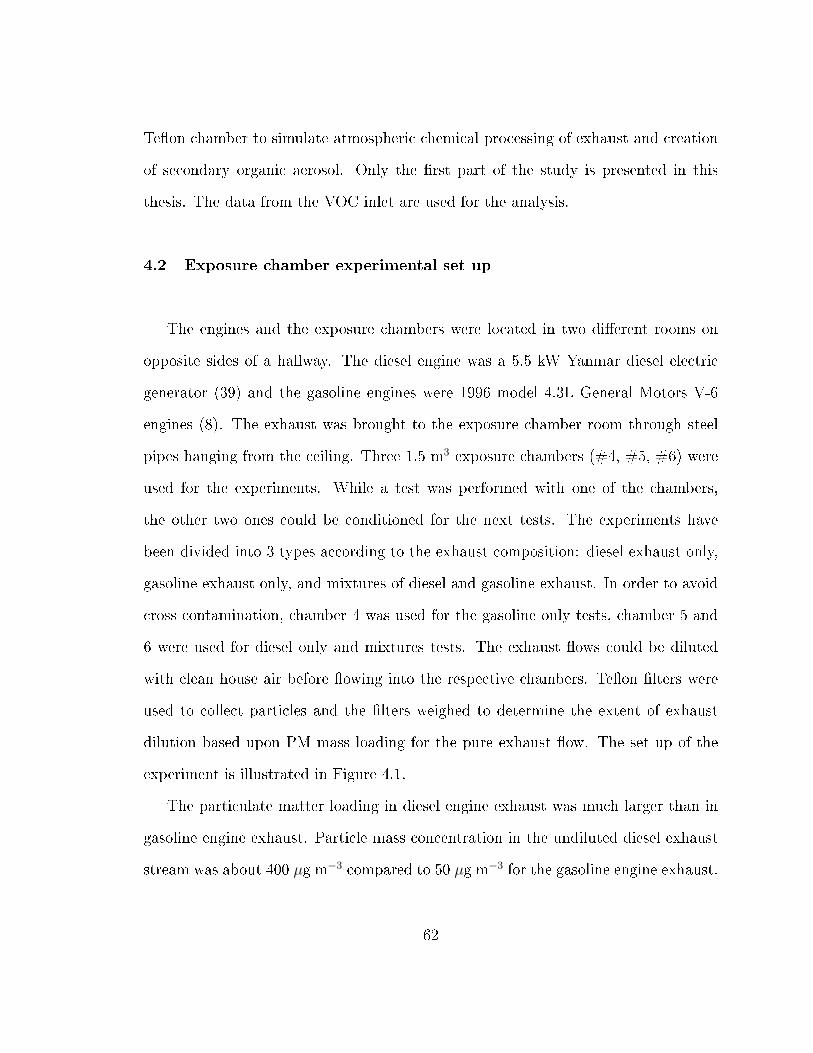
Te�on chamber to simulate atmospheric chemical processing of exhaust and creation
of secondary organic aerosol. Only the �rst part of the study is presented in this
thesis. The data from the VOC inlet are used for the analysis.
4.2 Exposure chamber experimental set up
The engines and the exposure chambers were located in two di�erent rooms on
opposite sides of a hallway. The diesel engine was a 5.5 kW Yanmar diesel electric
generator (39) and the gasoline engines were 1996 model 4.3L General Motors V-6
engines (8). The exhaust was brought to the exposure chamber room through steel
pipes hanging from the ceiling. Three 1.5 m3 exposure chambers (#4, #5, #6) were
used for the experiments. While a test was performed with one of the chambers,
the other two ones could be conditioned for the next tests. The experiments have
been divided into 3 types according to the exhaust composition: diesel exhaust only,
gasoline exhaust only, and mixtures of diesel and gasoline exhaust. In order to avoid
cross contamination, chamber 4 was used for the gasoline only tests, chamber 5 and
6 were used for diesel only and mixtures tests. The exhaust �ows could be diluted
with clean house air before �owing into the respective chambers. Te�on �lters were
used to collect particles and the �lters weighed to determine the extent of exhaust
dilution based upon PM mass loading for the pure exhaust �ow. The set up of the
experiment is illustrated in Figure 4.1.
The particulate matter loading in diesel engine exhaust was much larger than in
gasoline engine exhaust. Particle mass concentration in the undiluted diesel exhaust
stream was about 400 µg m−3 compared to 50 µg m−3 for the gasoline engine exhaust.
62

Figure 4.1. General plumbing schematic of the exposure chamber measurements
The mass loading of PM was used to determine the extent of dilution of the mixtures
in the chamber. A previous study was performed on the LRRI exposure chambers
(40) using the same particulate matter mass metric. The paarticule load is used to
represent the dilution of the exhaust. The engines were operated at di�erent loads
too. There were three types of loading: low, high and typical, all are detailed in
Table 4.1. A total of 23 experiments were performed and are summarized in Table
4.2. For example, the test 90D10G_27 is a mixture of diesel and gasoline run at a
typical gasoline engine load and a typical diesel engine load. The particle load is 90
µg m−3 for diesel and 10 µg m−3 for gasoline which corresponds to a dilution of 22%
of the undiluted diesel exhaust and 20% of the undiluted gasoline exhaust. This test
63

is considered as a low particle load which represents a well diluted exhaust.
Table 4.1. Engine load conditions
Engine Loading Condition Gas Diesel
Typical (average) Throttle (11%) 1123 RPM 4.5 kWLow Throttle (1%) 600 RPM 1.5 kWHigh Throttle (27 %) 1922 RPM 5.5 kW
64

Table 4.2. Experiments Summary
File name Particle Loading (µg/m3) Engine Load Type
type _ date Gas Diesel Gasoline : Diesel
diesel_27 0 292 Ø : T**
90D10G_27 12 370 T : Tgasoline_28 30 0 T : Ø
50D50G_m_28 50 73 T : T50D50G_l_28* 3 4 T : Tdiesel_28 0 8 Ø : Tgasoline_29 20 0 T : Ø40D5G_29 22 10 T : T200D25G_29 22 202 T : Tdiesel_29 0 34 Ø : Tgasoline_30 42 0 L : Ø400D50G_30 30 504 H : Ldiesel_30 0 288 Ø : L
80D10G_30* 45 16 H : L80D10G_01 4 114 L : Hdiesel_01 0 72 Ø : H
400D50G_01 33 304 L : H200D25G_02 42 236 H : H40D50G_02* 34 52 H : Hgasoline_02* 11 0 H : Ø400D50G_02 35 409 H : H300D5G_03 10 269 H : Hgasoline_03* 24 0 H : Ø
* The PTR-MS signal was low and the data cannot be used for analysis.** Engine loads: T=Typical, L=Low and H=High.
65

4.3 PTR-MS Sampling of Chambers
Of the 23 tests conducted, 6 tests had PTR-MS instrument problems and the
data collected was not useable. The main focus of the data analysis was to compare
the tests to determine the impact of engine loading and PM concentration variations
on the chamber mixtures compositions. As explained in the set-up section, engine
load and exhaust dilution were changed to obtain di�erent fractional composition of
diesel and gasoline in the exposure chambers. The PTR-MS used the IVOC/VOC
system but only the VOC data are reported here. The air was sampled from the
chambers through a heated PFA tube (1/8") and �ltered with a 2 µm Te�on �lter
to limit the intrusion of particles into the system. Those �lters were changed every
experiment or chamber run. The connection to the chamber is illustrated in Fig-
ure 4.2. Selected ions were measured and were grouped into eight categories. The
housekeeping ions represent the ions measured to verify that the drift tube is op-
erating properly. The housekeeping ions were m/z=21, m/z=30, and m/z=32 that
account for respectively H3O+, NO+, O+
2 , plus the m/z=39 and m/z=55 ions that
correspond to the water clusters. Then, there is the alkanes CnH2n+2(also called
para�ns or saturated hydrocarbons) and alkenes CnH2n (also called ole�n) group.
It is represented by the ion series m/z=43, 57, 71, 85, 99, 113, 127. The PTR-
MS can measure the alkanes ≥ C10 (decane) but those are likely to fragment into
m/z=43, m/z=57, m/z=71, and the most abundant alkanes from vehicle emissions
are ≤ C10 (24) so the PTR-MS does not provide representative signal for the alka-
nes. The alkenes ≥ C3 (propene) are measured by the PTR-MS and are abundant
in the exhaust (24). For the exhaust measurement the ions at m/z=43, m/z=57
66

and m/z=71 are more likely to represent the alkenes more than the alkanes. The
monoaromatics are represented by the m/z=79, 93, 107, 121, 135, 149, 163, 177, 191
ions. The tetrahydronaphthalenes group (91 + (n*14)) is represented by the ions at
m/z=105, 119, 133, 147, 161, 175, 189. The naphthalenes are represented by the
ions at m/z=129, m/z=143, m/z=157, and m/z=171. The PAHs are represented by
the ions at m/z=152, 155, 167. Those were not monitored in the tests Diesel_27,
Diesel_28, Gasoline_28,50D50G_m_28, 50D50G_l_28, 90D10G_27 (see Table 4.2.
There are two unknown families (CnH2n−1) and (67 +(n*14)) respresented by the ion
series m/z=69, 83, 97, 111, 125, 139, 153 and m/z=95, 109, 123, 137, 151, 165, 179
respectively. Those ions are reported in Table 4.3.
67

Figure 4.2. Pictures of the chamber exposure connection with the PTR-MS: Tubingsampling air from the chamber
68

Table 4.3. Ions measured with the PTR-MS during the exposure chamber experiment
m/z groups m/z groups m/z groups
21 H3O+ 81 137 67 +(n*14)30 NO+ 83 CnH2n−1 139 CnH2n−1
31 HCHO 85 alkanes/alkenes 143 naphthalene32 O+ 87 147 91 + (n*14)33 methanol 93 monoaromatic 149 monoaromatic39 Water cluster 95 67 +(n*14) 151 67 +(n*14)41 97 CnH2n−1 152 PAHs42 99 alkanes/alkenes 153 CnH2n−1
*
43 alkanes/alkenes 101 155 PAHs **
45 105 91 + (n*14) 157 naphthalene47 107 monoaromatic 161 91 + (n*14)51 109 67 +(n*14) 163 monoaromatic55 Water cluster 111 CnH2n−1 165 67 +(n*14)57 alkanes/alkenes 113 alkanes/alkenes 167 PAHs59 119 91 + (n*14) 171 naphthalene61 121 monoaromatic 175 91 + (n*14)63 123 67 +(n*14) 177 monoaromatic65 125 CnH2n−1 179 67 +(n*14)69 CnH2n−1 127 alkanes/alkenes 189 91 + (n*14)71 alkanes/alkenes 129 naphthalene 191 monoaromatic73 133 91 + (n*14)79 monoaromatic 135 monoaromatic* m/z=153 is accouting for the (CnH2n−1) group, but some PAHs may contribute tothat ion mass.
** m/z=155 is accounting for the PAHs group, but some fragment ions from alkanessuch as C16 may contribute to that ion mass.
4.3.1 Fuels composition and comparison to engine exhaust
For both diesel and gasoline, samples of the fuel used in the Lovelace experiments
were run through the PTR-MS in order to compare its composition before and after
combustion. Fuels were run using the dilution system at a Td=80, with an injection
69

rate of 20 µl hr−1 and a N2 �ow of 1008 sccm. A full mass spectrum of barscans
from m/z=21 to m/z=215 for diesel and from m/z=21 to m/z= 185 for gasoline were
measured. The diesel exhaust experiment selected for the comparison corresponds
to the less diluted (i.e with an higher particle loading) diesel only and run at a low
engine load which gives the highest signal: the diesel experiment from April 30th, with
a particle loading of 288 µg m−3. For the exhaust experiments only the selected ions
fron Table 4.3 were measured. The comparison of the diesel exhaust mass spectrum
and diesel fuel barscan is shown in Figure 4.3. The fuel has a more homogeneous
composition than the exhaust with signi�cant ion signal observed out to high mass
range whereas the exhaust displays rapidly decreasing ion signal intensity at larger
m/z. The diesel exhaust mass spectrum is dominated by ions from alkanes/alkenes
and monoaromatics, representing respectively 26% and 19% of the total ion signal
(sum of all ions measured except housekeeping). The (CnH2n−1) and (67+(n*14))
represent 4% and 2% respectively. In the fuel, the signal of alkanes/alkenes is still
dominant with 30.8% of the total ion signal. The (CnH2n) and the monoaromatic
group represent respectively 18.8% and 11.7% of the signal; the tetrahydronphthalenes
and (67+(n*14)) are less abundant accounting for respectively 9.4% and 6.1% of the
total signal. For m/z ≤ 75, in the exhaust the alkanes/alkenes and the oxygenated
ions dominate the signal and in the fuel only the alkane/alkene ions are dominant.
For each group of ions from m/z=75 to m/z=130, the monoaromatics are largely
dominant compared to the other organics for the exhaust but not in the fuel. For
m/z ≥ 130, in the exhaust the most abundant compounds are mainly the unknown
(67+(n*14)) group, then the monoaromatics. In the literature Vendeuvre et al (29)
measured by GCxGC the abundance of organics in diesel fuel. It appears that the
70

alkanes are also the most abundant group accounting for ±70% of the composition
by mass, then the monoaromatics ±18%, the diaromatics ±10% and the triaromatics
±1%. In Han et al. (26), the diesel exhaust composition (on a lean concentional
mode) was also dominated by alkanes by 27%, then alkenes 19% and aromatics 17%,
those percent are with respect to HC group. The alkanes were found to be relatively
more abundant in the fuel than in the exhaust.
The gasoline exhaust data selected for the comparison corresponds to the less di-
luted exhaust, run at a low engine load which o�ers the highest signal, gasoline_30.
The particle loading was 42 µg m−3. The mass spectrums are shown in Figure 4.4.
The gasoline fuel and exhaust mass spectrums are more similar than observed with
diesel. Gasoline is composed of lower molecular weight alkanes and aromatics (13).
Each ion group presents the same pattern, characterized by a large abundance of
monoaromatics compared to the other organic families. The fuel composition is dom-
inated by the monoaromatics representing 26% of the total ion signal. The second
more abundant group is the alkanes/alkenes accounting for 9.2%. In the gasoline
exhaust the monoaromatics are the most abundant representing 30% of the total ion
signal, and then the alkanes/alkenes represent 25%. Schmitz et al. (30) also con-
cluded in the dominant abundance in aromatics and alkanes, those accounting for
both a volume percent of ±45% of their gasoline fuel. The exhaust composition was
more dominated by aromatics in their study representing ±50% of the VOC pattern,
and alkenes and alkanes both accounting for ±23% of the VOC pattern.
71

Figure4.3.PTR-M
Smassspectraof
dieselexhaust(upper
panel)anddieselfuel(low
erpanel)at
Td=80.Show
nare
theioncountratesnormalized
tothereagentioncountrate
inMHz.
Exhaust
massspectraiscolorcoded
togroup
ionsinto
chem
ically
similar
functional
groups
72

Figure4.4.PTR-M
Smassspectraof
gasolineengineexhaust
(upper
panel)andgasolinefuel(low
erpanel).
Show
naretheioncountratesnormalized
tothereagentioncountrate
inMHz.
Exhaustmassspectraiscolorcoded
togroup
ionsinto
chem
ically
similar
functional
groups
73

4.3.2 Comparison of gasoline and diesel exhaust composition
The barscan of the diesel and gasoline fuel were really di�erent but the exhaust
mass spectrums are similar. The gasoline_30 and diesel_30 experiments (listed in
Table 4.1) were selected to compare the relative abundance of organics between the
two types of exhaust. The dilution for gasoline_30 was 16%, and for diesel_30 it
was 28%. The diesel engine exhaust is somewhat more dilute but still allows us to
draw general observations regarding compound abundance. The gasoline exhaust had
higher mixing ratios of VOCs than the diesel exhaust by a factor of ≈ 10. Although
there are more organics in the gasoline exhaust, the pattern of the mass spectrums
is similar for both diesel and gasoline exhaust. The abundance relative to benzene
(one of the compounds of the monoaromatic family) is not too di�erent except for
the higher masses as shown on Figure 4.5. Indeed, it seems hard to distinguish with
only PTR-MS measurements of the VOCs which exhaust would be diesel or gasoline
because they have a similar compound distribution.
Figure 4.5. Organics abundance relative to benzene for diesel and gasoline exhaust.Numbers in circles represent the ion mass
74

4.3.3 Particle and engine loading variations
The set up allowed the dilution of the diesel and gasoline exhaust in order to
obtain di�erent concentrations of particles in the exposure chambers. Experiments
with diesel only and gasoline only at di�erent particle loading and engine loading
were run and provide data to determine the e�ect of those two parameters on the gas
phase composition.
4.3.3.1 Diesel
The impact of the particle loading for diesel exhaust can be studied by comparing
three experiments run at a typical engine load with only a change in the particle
concentration due to di�erent dilutions. The diesel_27 experiment was run at a high
particle load of 292 µg m−3, the diesel_29 experiment was run at a low particle
load of 34 µg m−3 and the diesel_28 experiment was run at an even lower particle
loading of only 8 µg m−3. The �rst test is expected to have a higher VOC abundance
than the two other ones. The results are shown in Figure 4.6 and in Figure 4.7.
The abundance of organics for all the compound groups is signi�cantly lower in the
diesel_28 test than in the two other ones as expected. The abundance is lower by a
factor of four to up to �fteen depending on the group when comparing with the 34 µg
m−3 test mixture, and by the same range except the monoaromatics when comparing
with the 292 µg m−3 test mixture. Although we can notice that the large increase in
the particle loading from 34 µg m−3 to 292 µg m−3 is not characterized by a similar
increase in organic abundance, the monoaromatics are even signi�cantly lower by a
factor of 3. This could be due to the particle load that may not be representative of
75
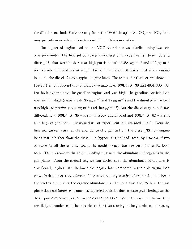
the dilution method. Further analysis on the IVOC data,the the CO2 and NOx data
may provide more information to conclude on this observation.
The impact of engine load on the VOC abundance was studied using two sets
of experiments. The �rst set compares two diesel only experiments, diesel_30 and
diesel_27, that were both run at high particle load of 288 µg m−3 and 292 µg m−3
respectively but at di�erent engine loads. The diesel_30 was run at a low engine
load and the diesel_27 at a typical engine load. The results for that set are shown in
Figure 4.8. The second set compares two mixtures, 400D50G_30 and 400D50G_02.
For both experiments the gasoline engine load was high, the gasoline particle load
was medium-high (respectively 30 µg m−3 and 35 µg m−3) and the diesel particle load
was high (respectively 504 µg m−3 and 409 µg m−3), but the diesel engine load was
di�erent. The 400D50G_30 was run at a low engine load and 400D50G_02 was run
at a high engine load. The second set of experiment is illustrated in 4.9. From the
�rst set, we can see that the abundance of organics from the diesel_30 (low engine
load) test is higher than the diesel_27 (typical engine load) tests by a factor of two
or more for all the groups, except the naphthalenes that are very similar for both
tests. The decrease in the engine loading increases the abundance of organics in the
gas phase. From the second set, we can notice that the abundance of organics is
signi�cantly higher with the low diesel engine load compared to the high engine load
test. PAHs increases by a factor of 4, and the other group by a factor of 10. The lower
the load is, the higher the organic abundance is. The fact that the PAHs in the gas
phase does not increase as much as expected could be due to some partitioning: as the
diesel particles concentration increases the PAHs compounds present in the mixture
are likely to condense on the particles rather than staying in the gas phase. Increasing
76

Figure 4.6. Impact of diesel particle loading on organics abundance at typical engineloading (total organic abundance).
the particle loading would enhance the partitioning. Further comparisons between
the HR-ToF-AMS data and the IVOC data should provide more evidence regarding
the partitioing phenomena since the IVOC inlet allows more accurate measurements
of the higher molecular weight compounds as the PAHs.
4.3.3.2 Gasoline
As for diesel, the analysis of the impact of the particle load and engine load on
the organic abundances was performed selecting a set of three gasoline only type of
experiments: gasoline_28, gasoline_29 and gasoline_30 that were run respectively
at 30 µg m−3 and a typical engine load, 20 µg m−3 and a typical engine load, and
42 µg m−3 and a low engine load. We expect that the low dilution (higher PM
concentration) and lower engine load would result in higher organic abundance in the
mixture. The results are shown in Figure 4.10. We can see that for the gasoline_30
77

Figure 4.7. Impact of diesel particle loading on organics abundance at typical engineloading.
Figure 4.8. Impact of diesel engine loading on the organic abundance in a diesel onlymixture, at a constant particle loading
78

Figure 4.9. Impact of diesel engine loading on the organic abundance in a gasolineand diesel mixture, at a constant particle loading for both diesel and gasoline
test (low engine load) the organic abundance is higher than both gasoline_28 and
gasoline_29 by a factor of 5 to 10 and 3 to ten respectively, depending on the group we
are looking at. Similar to the diesel engine, lower engine load increases the abundance
of organics.
The two typical engine loading experiments show the opposite of the expected
result: as the particle concentration increases there is a decrease in the abundance of
organics. This interesting observation could be explained by dilution issues that might
occur so that one of those two gasoline experiments was not diluted as we thought.
It also could come from a leak in the sampling plumbing that would result in lower
count for the gasoline_28 so that the total abundance would be underestimated.
79

Figure 4.10. Impact of particle loading and engine loading variations for gasoline onlymixtures.
4.3.3.3 Mixture with variation in the gas and particles loadings
The following three experiments were run at typical engine load and at a same
gasoline particle load of 20 µg m−3. The variable in this set of experiments is the diesel
particle load. The Gasoline_29 was only gasoline, the 45D5G_29 was a low diesel
particle load of 10 µg m−3 and the 200D25G was a medium diesel particle load of 202
µg m−3. This comparison uses the VOC data to determine the variations in the gas
phase, and the HR-ToF-AMS data to determine the variations in the particle phase.
The particle concentration were calculated using the standard fragmentation table
(41), and the collection e�ciency of CE=0.5). There is a noticeable decrease in the
organic compounds in the gas phase as the fraction of diesel (i.e the particle loading)
increases. The decrease is not proportional to the fraction of diesel added because
between 10 µg m−3 and 202 µg m−3 the total group abundance for the di�erent groups
of organics does not vary signi�cantly. Increasing the fraction of diesel exhaust in the
80

Figure 4.11. Impact of the increase in the fraction of diesel on the organic abundanceof a mixture, at a constant gasoline particle load of 20 µg m−3 and at a typical engineloading for both diesel and gasoline.
mixture decreases the amount of VOCs in the gas phase as illustrated in Figure 4.11.
A factor of decrease is barely observed for the naphthalenes and PAHs compared
to the factor of 3 or more for the other families. It can be explained by the larger
abundance of heavier compounds in diesel than in the gasoline. The total PM mass
concentration increases signi�cantly as the diesel fraction increases as illustrated in
Figure 4.12. The total particle mass concentration includes PAHs and organic mass
concentrations. This shows that the gasoline engine was the major source of VOCs
and the diesel engine the major source of PM. For further analysis the comparison
of the gas phase data obtained with IVOC system and the HR-ToF-AMS data could
also povide evidences on the partitioning phenomena that can occur with the larger
molecular weight compounds like the PAHs.
81

Figure 4.12. HR-ToF-AMS measurements. Impact of the increase in the fraction ofdiesel in the particles concentrations of a mixture, at a constant gasoline particle loadof 20 µg m−3 and a typical engine loading for both diesel and gasoline.
82

Chapter 5. Conclusions
The �rst part of the laboratory experiments was to evaluate the accuracy of the
dynamic dilution system. This was done by comparing mixtures made from infusing
benzene, p-xylene, toluene, and 1,3,5-trimethylbenzene using the syringe pump to
a test mixture made by diluting a multicomponent gas standard containing these
compounds. The gas standard is what is normally used to calibrate the PTR-MS.
The experiments involved varying the infusion rate from 0.1 µl hr−1 to 50 µl hr−1 as
well as varying the injection manifold temperature from room temperature to 70 ◦C.
The compounds with the lower vapor pressure, p-xylene and 1,3,5-trimethylbenzene,
yielded good results with less than 10% di�erence between the measured mixing ratio
using the gas phase standard instrument sensitivity and the expected mixing ratios
calculated from the infusion rate and dilution gas �ow rate. The experiments with
benzene and toluene suggest that injection manifold temperature needs to be adjusted
to keep the compound vapor pressure below 100 Torr. At high manifold temperatures
and low infusion rates, signi�cantly more benzene and toluene (> 20%) was measured
than expected. Excessive mass loss due to evaporation of the liquid from the syringe
needle is the likely cause. Increasing the infusion rate would mitigate this problem.
This evaporative loss problem will set a limit to the lowest possible infusion rate and
wil be compound dependent. For future work, additional tests with other compounds
83

should be performed to con�rm the 100 Torr upper limit and to verify the lower limit
infusion rates.
Acenaphthylene, acenaphthene and biphenyl sensitivity tests were performed at
Td=80 using the dynamic dilution system and resulted in normalized count rate sen-
sitivities of respectively 3.1 ± 0.3, 3.2 ± 0.3 and 3.2± 0.6 Hz per ppbV MHz H3O+.
These compounds did not fragment and so can be monitored at m/z=153, m/z=155,
and m/z=155 respectively. The work demonstrated that it is possible to make liquid
standards from these solids and measure them with the PTR-MS. The solvent used
in these tests was dichloromethane. While this compound doesn't react with H3O+,
ions resulting from its use were observed. The ions m/z=49 and m/z=51 were at-
tributed to the 35Cl and 37Cl isotopes of CH2Cl+. The m/z=31 ion was also observed.
Production of these ions likely resulted when air from the drift tube di�used into the
ion source. For further work, these standards should be run through the thermal
desorption IVOC system for comparison.
The second part of the laboratory experiments was to study fragmentation pat-
terns of monoaromatic compounds and several polyaromatic hydrocarbons usually
present in gasoline and diesel exhaust. Typically the PTR-MS is operated at Townsend
numbers between 120 and 150 to avoid water cluster formation in the drift tube. Re-
sults from these experiments show that fragmentation occurs for many monoaromatic
compounds at those Tds. The compounds that have ethyl groups attached to the ben-
zene ring fragment at Td=150. Compounds with an isopropyl group attached to the
benzene ring showed little fragmentation at Td=80 and high fragmentation at Td=120
and Td=150. The compounds that have a methyl group attached to the benzene ring
84

did not fragment. Such fragmentation patterns may produce interferences with the
measurement of benzene at m/z=79 and toluene at m/z=93 in vehicle exhaust. The
compounds that are composed of longer chain alkyl groups attached to the benzene
ring also fragmented. It was observed that fragmentation of these compounds can
produce fragment ions at m/z=43 and so may produce an interference with the mea-
surement of alkanes in vehicle exhaust. The PAHs that were studied were dissolved
into a dichloromethane solution. No fragmentation pattern were noticed except for
the tetrahydronaphthalene that fragmented into m/z=91 at Td=150. The laboratory
experiments prove that low molecular weight PAH compounds can be measured by
the PTR-MS and that these compounds have similar normalized sensitivity of 3.2 Hz
per ppbV MHz H3O+ at Td=80. For further works, some tests should be performed
on additional compounds, also usually present in diesel and gasoline exhaust, to en-
large the fragmentation pattern list.
The Lovelace experiment was divided into two set of experiments. The �rst part
focuses on the gas phase and particle phase composition of mixture of gasoline and
diesel exhausts from exposure chambers. The results on the gas phase measurements
by the VOC system were detailled in this thesis. The diesel fuel was composed
mainly mainly of ions from the alkanes/alkenes group and made up 31% of the total
ion signal. In the diesel exhaust, the alkanes/alkenes were still the most abundant
group representing 26% of the total ion signal, but also contained a larger fraction
of monoaromatics (19% of the total ion signal) than in the fuel (11% of the total ion
signal) especially for the ion range between m/z=75 and m/z=130. The gasoline fuel
was mostly composed of monoaromatics representing 26% of the total ion signal. The
85

gasoline exhaust composition was also dominated by aromatics representing 30% of
the total ion signal, but also contained a larger fraction of alkanes/ alkenes (25% of
the total ion signal) than in the fuel (9% of the total ion signal).
Experiments were run at three di�erent engine loading: high, typical or low.
Both gasoline and diesel exhaust gas phase composition was in�uenced by the engine
loading. A decrease in the engine loading increases the abundance of the organics. For
the unmixed exhaust experiments (gasoline only or diesel only) at high dilutions were
PM mass concentrations were less than 8.5% of the undiluted exhaust, the change in
VOC concentration was consistent with the extent of exhaust dilution as measured
by the change in PM mass concentration.
Three gasoline/diesel exhaust mixtures for which the fraction of diesel increased
were compared. As the fraction of diesel increased the abundance of VOC decreased
for high dilution conditions (from 20 µg m−3 of gasoline only to a mixture of 20
µg m−3 of gasoline and 10 µg m−3 of diesel). As the fraction of diesel increased
the abundance of VOC remained the same for less diluted air (from 20 µg m−3 of
gasoline and 10 µg m−3 of diesel to 20 µg m−3 of gasoline and 202 µg m−3 of diesel).
Those results showed that the gasoline exhaust mainly contributed to the abundance
of VOC in the gas phase while the diesel exhaust contributed to the particle phase.
All the data from the Lovelace experiment that were presented in this thesis were
representative of the signal count but were not in mixing ratio. The next step would
be to generate the results in ppbv using the sensitivities obtained during calibration
tests. For further work the analysis of the IVOC data would be needed to provide
additional information on the PAHs and the less volatile compounds that did not
present high counts through the VOC system. The present analysis provides some
86

interesting evidence of gas to particle partitioning of PAH compounds, but further
investigation is suggested using data from the IVOC sampling system and results
from the AMS instrument.
87

REFERENCES
(1) Pope CA and Dockery DW, �Health E�ects of Fine Particulate Air Pollution
: Lines that Connect,� Journal of Air and Waste Management Association,
vol. 56, pp. 709�742, 2006.
(2) Brunekreef B, Janssen NAH, de Hartog J, Harssema H, Knape M, and Van Vliet
P, �Air Pollution from Truck Tra�c and Lung Function in Children Living near
Motorways,� Epidemiology, vol. 8, no. 3, pp. 298�303, 1997.
(3) Campen MJ, Lund AK, Doyle-Eisele ML, McDonald JD, Knuckles TL, Rohr
AC, Knipping EM, and Mauderly JL, �A comparison of vascular e�ects from
complex and individual air pollutants indicates a role for monoxide gases and
volatile hydrocarbons.,� Environmental health perspectives, vol. 118, pp. 921�7,
July 2010.
(4) Cho SH, Tong H, McGee JK, Baldauf RW, Krantz QT, and Gilmour MI, �Com-
parative toxicity of size-fractionated airborne particulate matter collected at
di�erent distances from an urban highway.,� Environmental health perspectives,
vol. 117, pp. 1682�9, Nov. 2009.
(5) Dockery DW, Pope CA, Xu X, Spengler JD, Ware JH, Fay ME, Benjamin G.
Ferris J, and Speizer FE, �An association between air pollution and mortality
88

in six U.S. cities,� The New England Journal of Medecine, vol. 329, no. number
24, 1993.
(6) Dockery DW, Luttmann-Gibson H, Rich DQ, Link MS, Mittleman Ma, Gold DR,
Koutrakis P, Schwartz JD, and Verrier RL, �Association of Air Pollution with In-
creased Incidence of Ventricular Tachyarrhythmias Recorded by Implanted Car-
dioverter De�brillators,� Environmental Health Perspectives, vol. 113, pp. 670�
674, Feb. 2005.
(7) Gilmour MI, McGee J, Duvall RM, Dailey L, Daniels M, Boykin E, Cho SH,
Doer�er D, Gordon T, and Devlin RB, �Comparative toxicity of size-fractionated
airborne particulate matter obtained from di�erent cities in the United States.,�
Inhalation toxicology, vol. 19(Supp.l, pp. 7�16, Jan. 2007.
(8) McDonald JD, Reed MD, Campen MJ, Barrett EG, Seagrave J, and Mauderly
JL, �Health e�ects of inhaled gasoline engine emissions.,� Inhalation toxicology,
vol. 19 Suppl 1, pp. 107�16, Jan. 2007.
(9) Peters A, Von Klot S, Heier M, Trentinaglia I, Hörmann A, Wichmann HE, and
Löwel H, �Exposure to Tra�c and the Onset of Myocardial Infarction,� The New
England Journal of Medecine, vol. 351, no. 17, pp. 1721�1730, 2004.
(10) Seagrave J, McDonald JD, Gigliotti AP, Nikula KJ, Seilkop SK, Gurevich M,
and Mauderly JL, �Mutagenicity and in vivo toxicity of combined particulate
and semivolatile organic fractions of gasoline and diesel engine emissions.,� Tox-
icological sciences, vol. 70, pp. 212�26, Dec. 2002.
(11) Lai C, Chen K, Ho Y, and Chou M, �Characteristics of C2-C15 hydrocarbons
89

in the air of urban Kaohsiung, Taiwan,� Atmospheric Environment, vol. 38,
pp. 1997�2011, Apr. 2004.
(12) Schauer JJ, Kleeman MJ, Cass GR, and Simoneit BRT, �Measurement of Emis-
sions from Air Pollution Sources. 5. C1-C32 Organic Compounds from Gasoline-
Powered Motor Vehicles,� Environmental Science & Technology, vol. 36,
pp. 1169�1180, 2002.
(13) Zielinska B, Sagebiel JC, Harsh�eld G, Gertler AW, and Pierson WR, �Volatile
Organic compounds up to C20 emitted from motor vehicles; measurement meth-
ods,� Atmospheric Environment, vol. 30, no. 12, pp. 2269�2286, 1996.
(14) Rogge WF, HIldemann LM, Mazurek MA, and Cass GR, �Mathematical mod-
eling of atmospheric �n particle-associated primary organic compound concen-
trations,� 1996.
(15) Robinson AL, Donahue NM, Shrivastava MK, Weitkamp Ea, Sage AM, Grieshop
AP, Lane TE, Pierce JR, and Pandis SN, �Rethinking organic aerosols:
semivolatile emissions and photochemical aging.,� Science, vol. 315, pp. 1259�62,
Mar. 2007.
(16) Presto A, Miracolo M, Kroll JH, Worsnop DR, Robinson AL, and Donahue
NM, �Intermediate-volatility organic compounds: a potential source of ambi-
ent oxidized organic aerosol.,� Environmental Science & Technology, vol. 43,
pp. 4744�9, July 2009.
(17) Odum JR, Ho�mann T, Bowman F, Collins D, Flagan RC, and Seinfeld JH,
90

�Gas/Particle Partitioning and Secondary Organic Aerosol Yields,� Environ-
mental Science & Technology, vol. 30, pp. 2580�2585, Jan. 1996.
(18) Seinfeld JH and Pandis SN, Atmospheric Chemistry and Physics: From Air
Pollution to Climate Change. Wiley-Interscience, 2006.
(19) de Gouw J and Warneke C, �Measurements of volatile organic compounds in the
earth's atmosphere using proton-transfer-reaction mass spectrometry,� Wiley
Periodicals, Inc, vol. 26, pp. 223�257, 2007.
(20) Dasgupta PK, Li J, Zhang G, Luke WT, McClenny WA, Stutz J, and Fried
A, �Summertime Ambient Formaldehyde in Five U.S. Metropolitan Areas:Â
Nashville, Atlanta, Houston, Philadelphia, and Tampa,� Environmental Science
& Technology, vol. 39, pp. 4767�4783, July 2005.
(21) Cogliano V, Grosse Y, Baan R, Straif K, Secretan B, and Ghissassi FE, �Advice
on formaldehyde and glycol ethers,� The Lancet Oncology, vol. 5, p. 528, Sept.
2004.
(22) Mohamed MF, Kang D, and Aneja VP, �Volatile organic compounds in some
urban locations in United States,� Chemosphere, vol. 47, pp. 863�882, June 2002.
(23) Ho KF, Lee SC, Ho WK, Blake DR, Cheng Y, Li YS, Ho SSH, Fung K, Louie
PKK, and Park D, �Vehicular emission of volatile organic compounds (VOCs)
from a tunnel study in Hong Kong,� Atmospheric Chemistry and Physics, vol. 9,
pp. 7491�7504, Oct. 2009.
(24) Lough GC, Schauer JJ, Lonneman Wa, and Allen MK, �Summer and winter
nonmethane hydrocarbon emissions from on-road motor vehicles in the Mid-
91

western United States.,� Journal of the Air & Waste Management Association,
vol. 55, pp. 629�46, May 2005.
(25) McGaughey GR, Desai NR, Allen DT, Seila RL, Lonneman Wa, Fraser MP,
Harley Ra, Pollack AK, Ivy JM, and Price JH, �Analysis of motor vehicle emis-
sions in a Houston tunnel during the Texas Air Quality Study 2000,� Atmo-
spheric Environment, vol. 38, pp. 3363�3372, June 2004.
(26) Han M, Assanis DN, Jacobs TJ, and Bohac SV, �Method and Detailed Anal-
ysis of Individual Hydrocarbon Species From Diesel Combustion Modes and
Diesel Oxidation Catalyst,� Journal of Engineering for Gas Turbines and Power,
vol. 130, no. 4, p. 042803, 2008.
(27) Siegl W, Hammerle H, Hermann H, Wenclawiak B, and Luers-Jonge B, �Or-
ganic emissions pro�le for a light-duty diesel vehicle,� Atmospheric Environment,
vol. 33, pp. 797�805, Feb. 1999.
(28) Schauer J, Kleeman M, Cass GR, and Simoneit BRT, �Measurement of emissions
from air pollution sources. 2. C1 through C30 organic compounds from medium
duty diesel trucks,� Science & Technology, vol. 33, no. 10, pp. 1578�1587, 1999.
(29) Vendeuvre C, Ruiz-Guerrero R, Bertoncini F, Duval L, Thiébaut D, and Hennion
MC, �Characterisation of middle-distillates by comprehensive two-dimensional
gas chromatography (GCxGC): A powerful alternative for performing various
standard analysis of middle-distillates,� Journal of Chromatography A, vol. 1086,
pp. 21�28, Sept. 2005.
(30) Schmitz T, Hassel D, and Weber FJ, �Determination of VOC-components in
92

the exhaust of gasoline and diesel passenger cars,� Atmospheric Environment,
vol. 34, pp. 4639�4647, Jan. 2000.
(31) Lindinger W, Hansel A, and A. Jordan , �On-line monitoring of volatile or-
ganic compounds at pptv levels by means of Proton-Transfer-Reaction Mass
Spectrometry (PTR-MS) Medical applications, food control and environmental
research,� International Journal of Mass Spectrometry, vol. 173, pp. 191�241,
1998.
(32) Jobson BT and McCoskey JK, �Sample drying to improve HCHO measure-
ments by PTR-MS instruments: laboratory and �eld measurements,� Atmo-
spheric Chemistry and Physics, vol. 10, pp. 1821�1835, Feb. 2010.
(33) Faiola CL, Erickson MH, Fricaud VL, Jobson BT, and VanReken TM, �Quanti�-
cation of biogenic volatile organic compounds with a �ame ionization detector
using the e�ective carbon number concept,� Atmospheric Measurement Tech-
niques, vol. 5, pp. 1911�1923, Aug. 2012.
(34) Buhr K, van Ruth S, and Delahunty C, �Analysis of volatile �avour compounds
by Proton Transfer Reaction-Mass Spectrometry: fragmentation patterns and
discrimination between isobaric and isomeric compounds,� International Journal
of Mass Spectrometry, vol. 221, pp. 1�7, Nov. 2002.
(35) Jobson B, Alexander M, Maupin G, and Muntean G, �On-line analysis of organic
compounds in diesel exhaust using a proton transfer reaction mass spectrometer
(PTR-MS),� International Journal of Mass Spectrometry, vol. 245, pp. 78�89,
Aug. 2005.
93

(36) Barker J, Mass Spectrometry: Analytical Chemistry by Open Learning. Wiley,
1999.
(37) Foureman G, �Concise International Chemical Assessment Document 18:
CUMENE,� tech. rep., WorldHealthOrganization, Research Triangle Park, NC,
USA, 2005.
(38) McLa�erty FW and Turecek F, Interpretation of Mass Spectra. University Sci-
ence Books, Mill Valley, California, 4th ed., June 1994.
(39) McDonald JD, Campen MJ, Harrod KS, Seagrave J, Seilkop SK, and Mauderly
JL, �Engine-operating load in�uences diesel exhaust composition and cardiopul-
monary and immune responses,� Environmental health perspectives, vol. 119,
pp. 1136�41, Aug. 2011.
(40) McDonald JD, Barr EB, White RK, Chow JC, Schauer JJ, Zielinska B, and
Grosjean E, �Generation and characterization of four dilutions of diesel engine
exhaust for a subchronic inhalation study.,� Environmental Science & Technol-
ogy, vol. 38, pp. 2513�22, May 2004.
(41) Allan JD, Delia AE, Coe H, Bower KN, Alfarra M, Jimenez JL, Middlebrook
AM, Drewnick F, Onasch TB, Canagaratna MR, Jayne JT, and Worsnop DR,
�A generalised method for the extraction of chemically resolved mass spectra
from Aerodyne aerosol mass spectrometer data,� Journal of Aerosol Science,
vol. 35, pp. 909�922, July 2004.
94