1

Measuring Absorption and Scattering

Properties for Spider Filters

Kristen McKee

Project Advisor: Professor John Ruhl

Physics Department

Case Western Reserve University

May 2, 2014

2

Table of Contents

Executive Summary…………………………….…….3

Background……………………………………….….3

Introduction…………………………………………..4

Objectives…………………………………………….7

Review of Previous Work……………………………..7

Design and Experimental Set-up……..........................11

Methods……………………………………………... 16

Procedure and Data Analysis…………………………19

Results…………………………………………..…….29

Conclusion…………………………………………....31

Sources……………………………………………….32

3

Executive Summary

The Cosmic Microwave Background (CMB) is a blackbody of thermal radiation leftover

from the Big Bang, which today is shifted into the range of microwave photons. The Spider

experiment is designed to detect a very small polarization signal in the CMB, which would

signify the existence of gravity waves in the early universe. Since the experiment is only trying

to detect in certain bands of microwave photons (centered at 90 GHz and 150 GHz), it contains

many filters which screen out photons outside of these ranges.

Filters ideally transmit all photons within the desired microwave frequency bands to the

detector; however, this is not always what happens. Some photons can be absorbed, reflected, or

scattered by the filter rather than being transmitted to the detector. If the fraction of scattering,

absorption, and reflection of these photons is too high, it can cause problems in the experiment.

In this project, I built and debugged a novel test setup to enable measurements of absorption,

reflection, and scattering properties of Spider filters. I then tested two different Spider low pass

filters in order to measure the fraction of incident photons which were scattered, absorbed, and

reflected by each of the filters.

Background

In the very early universe, baryonic matter formed a hot, ionized plasma. However, as the

universe cooled and matter became neutral, photons were scattered from electrons less and less

frequently. After their last scattering, photons became free to move throughout the universe

4

independently from baryonic matter. The photons from the time of last scattering which we

observe today (red-shifted to microwaves) compose the Cosmic Microwave Background (CMB).

The CMB was first measured by Penzias and Wilson in 1965 [1]. Since this discovery,

many experiments have engaged in measuring various properties of the CMB. In 1992, the

COBE satellite first measured small anisotropies in the intensity of the CMB and showed that the

power spectrum of the CMB was very close to that of a uniform blackbody [2]. This

measurement supported the theory of inflation in the early universe. The experiments WMAP [3]

and Boomerang [4] both measured the temperature anisotropies in the CMB, providing precise

measurements of the angular power spectrum. Measurements of these anisotropies are significant

because they provide information about important cosmological parameters. The goal of the

SPIDER experiment is to detect a small polarization signal in the CMB which would signify the

existence of gravity waves in the early universe.

Introduction

Optical filters are essential components of CMB experiments such as Spider. A filter is a

device which blocks out photons in specific frequency ranges. Since the Spider experiment is

measuring microwave photons, it has detectors which are sensitive to bands centered at 90 GHz

and 150 GHz, with 20% bandwidth. The goal of the filters is thus to screen out all photons which

do not lie in the frequency bands around 90 and 150 GHz and to transmit to the detector all

photons which are in these bands.

5

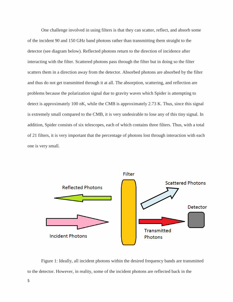
One challenge involved in using filters is that they can scatter, reflect, and absorb some

of the incident 90 and 150 GHz band photons rather than transmitting them straight to the

detector (see diagram below). Reflected photons return to the direction of incidence after

interacting with the filter. Scattered photons pass through the filter but in doing so the filter

scatters them in a direction away from the detector. Absorbed photons are absorbed by the filter

and thus do not get transmitted through it at all. The absorption, scattering, and reflection are

problems because the polarization signal due to gravity waves which Spider is attempting to

detect is approximately 100 nK, while the CMB is approximately 2.73 K. Thus, since this signal

is extremely small compared to the CMB, it is very undesirable to lose any of this tiny signal. In

addition, Spider consists of six telescopes, each of which contains three filters. Thus, with a total

of 21 filters, it is very important that the percentage of photons lost through interaction with each

one is very small.

Figure 1: Ideally, all incident photons within the desired frequency bands are transmitted

to the detector. However, in reality, some of the incident photons are reflected back in the

6

direction of the source, some photons are absorbed by the filter, and some photons are scattered

away from the detector when they pass through the filter.

Methods have already been developed for determining the transmission and reflectance

of these optical materials. One can test transmission by shining microwave photons at the

material and aligning a detector at the opposite side of the material. Similarly, reflectance can be

determined by shining microwave photons onto the material and aligning a detector on the same

side of the material in order to measure the percentage of incident photons which are reflected

back towards the source.

Although the methods for determining transmission and reflectance properties are fairly

straightforward, determining the absorption and scattering properties of these devices has always

posed more of a problem. While one can use measurements of transmission and reflectance

properties to infer the amount of scattering plus absorption together, it is complicated to

differentiate between scattered photons and absorbed photons. This is because absorbed photons

stay in the material and thus cannot be directly measured. The scattered photons, on the other

hand, consist of all photons which make it through the window/ filter material but not to the

detector. Consequently, they are projected onto such a wide area of space that it is very difficult

to make precise measurements of them [5]. For this project, I am building, debugging, and using

a novel test setup to enable measurements of absorption and scattering properties for two Spider

low pass filters.

7

Objectives

The first objective was to use SolidWorks to design a test setup for measuring the

absorption, scattering, and reflection of millimeter waves from various optical devices. This set-

up consisted of a scatterometer built in the lab as well as a thermal blackbody load for a source

and a test dewar containing the detector. The next goal was to assemble and debug the test setup

and use it to make measurements of absorption, reflection, and scattering properties for Spider

filters. After measuring the desired optical properties, the next objective was to write Matlab

code to analyze the data and determine the amount of absorption, scattering, and reflection

caused by each of the optical materials that are tested. Data was taken for several optical devices,

but the data analysis was eventually focused on two different Spider low pass filters.

Review of Previous Work

Many people in the Spider collaboration were concerned that there was too much

uncertainty in the amount of absorption and scattering from the Spider windows. The entire

Spider experiment resides inside of a cryostat under vacuum. The purpose of the windows is to

provide a way for photons to enter the cryostat. Thus, they must be composed of materials which

are strong enough to hold vacuum but are also microwave-transparent. For Spider the windows

are composed of ultra-high-molecular-weight polyethylene (UHMWPE). Spider collaboration

members at Caltech came up with the idea to test the scattering and reflection properties of the

Spider windows and other optical devices using a test baffle, or hollow metal cylinder, as a

scatterometer. In this setup, the test baffle is attached to the window of a test dewar. Underneath

the baffle is a thermal cold load. Photons sourced by the cold load travel through the baffle into

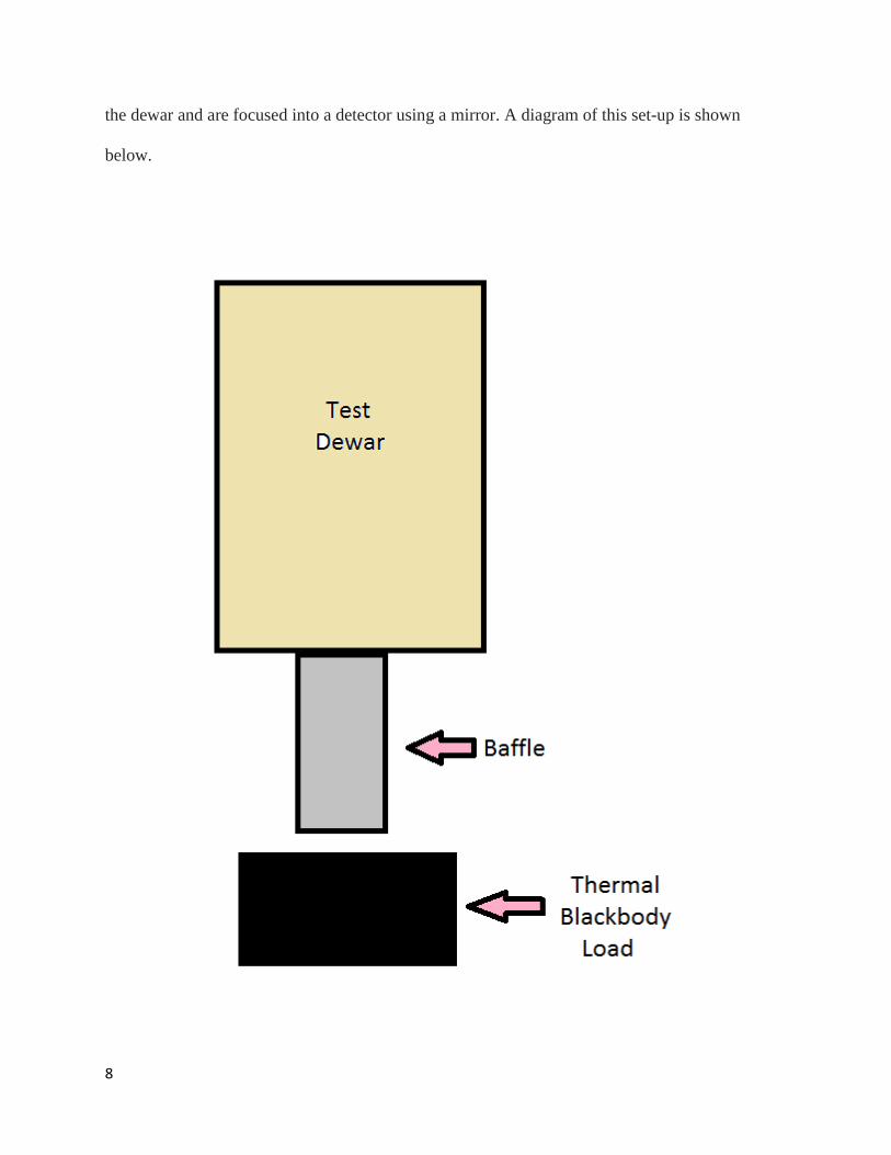
8

the dewar and are focused into a detector using a mirror. A diagram of this set-up is shown

below.

9

Figure 2: A diagram of the set-up that the Caltech Spider collaborators used to test the

absorption, reflection, and scattering caused by the Spider ultra-high-molecular-weight

polyethylene (UHMWPE) windows. This set-up consists of a thermal blackbody load which

serves as the source, a “baffle,” or hollow cylinder, for photons to travel through into the dewar,

and a test dewar which contains the detector.

Leaving the inside of the baffle shiny will cause scattered photons to be reflected off the

sides of the baffle and thus remain in the baffle. However, blackening the inside of the baffle will

cause scattered photons to be absorbed by the side of the baffle, and hence they will not make it

to the dewar and will not be detected. By performing this test with the baffle both shiny and

blackened, one can then separate the scattered photons from the absorbed photons, thus

achieving the goal of determining these properties.

Spider Collaboration members at Caltech used this principle to determine the scattering

and absorption for a few of the optical devices used in Spider. They first tested a shader, which is

a type of filter. They found a value of absorption minus reflection of around 0.3 %, and minimal

scattering from the shader. They also tested a Spider hot pressed filter and found that absorption

minus reflection was around 0.8%, which indicated some amount of absorption and reflection.

However, scattering was still minimal. They used this same procedure for testing an ultra-high-

molecular-weight polyethylene (UHMWPE) Spider window and found that absorption minus

reflection was around 0.7%, but there was a negligible amount of scattering. Similar tests of

foam windows provided inconclusive results, as there were large variations among each of the

measurements [6].

10

These results from the Caltech Spider collaborators proved that using this test set-up was

a possible way to find out information about absorption and scattering properties for various

optical devices. However, their set-up was thoroughly debugged, as it was only constructed

quickly to see if the concept would work. In addition, measurements were not repeated

extensively. They also had some problems including condensation on the thermal load, which

caused some of the signal to be absorbed.

The goal of my project was to create and refine a similar test set-up which would enable

systematic testing of the absorption, reflection, and scattering properties for various optical

devices. This refined set-up was conducive to systematic repetition of measurements to allow for

more accurate results. In addition, I also took extra measurements using a chopper wheel in order

to take into account a possible spillover of the main beam.

In my setup, I was also able to separate the percentage of absorption, reflection and

scattering caused by the filter of interest. This is important because each of these types of

photons can create different, undesirable effects. For example, reflected photons can be reflected

back into the focal plane of the detector and cause a false signal. In addition, since Spider

observes very close to sources of polarization contamination, such as the galaxy, it is necessary

to limit the amount of light that is observed at these wide angles on the sky. Scattered photons

are a problem because they contribute to this signal when they are scattered to wide angles.

11

Design and Experimental Set-Up

The set-up for this experiment consisted of a scatterometer built in the lab as well as a

thermal blackbody load for a source and a test dewar used for photon detection. A diagram of the

full set-up is shown below.

12

Figure 3: A diagram of the experimental set-up. It consists of a thermal blackbody load,

constructed out of HR-10, a microwave absorbing material. The scatterometer consists of a

“baffle” (hollow cylinder) which is covered in either shiny (aluminum) or black (HR-10)

material, and a shelf to put the filter on. The large blue device is a cross section model of the test

dewar. The entire dewar was kept under vacuum. The cylinder at the bottom of the dewar is the

window, which holds vacuum but allows microwave photons to pass through it. The test dewar

also contains an elliptical mirror (left) for focusing photons into the detector (right).

In this experimental set-up, the thermal blackbody load serves as a source of incident

photons. Measurements were made with this load functioning as a 77 K blackbody and again as a

300 K blackbody. In order to create a 300 K blackbody, a large square piece (approximately 1’x

1’) of HR-10 (a microwave-absorbing material) was placed under the baffle at room temperature.

In order to create a 77K blackbody, a small rectangular bucket lined with HR-10 was filled with

liquid nitrogen and placed directly under the baffle.

The scatterometer consisted of a hollow cylinder (called a “baffle”) and a shelf on which

to rest the filter so that it remained directly above the baffle opening during measurements.

Measurements were taken with the baffle being both shiny and then black. “Shiny” means that

the inside of the baffle is aluminum and thus all photons which scatter to the side of the baffle

will be reflected and continue to propagate within the baffle interior. On the other hand, “black”

means that the inside of the baffle was covered in HR-10, and thus all microwave photons which

were scattered to the side of the baffle were absorbed by this material and thus ceased to

propagate within the baffle. Two separate baffles (one shiny and one black) were constructed for

this purpose, and thus it was necessary to detach and change the baffle when switching between

13

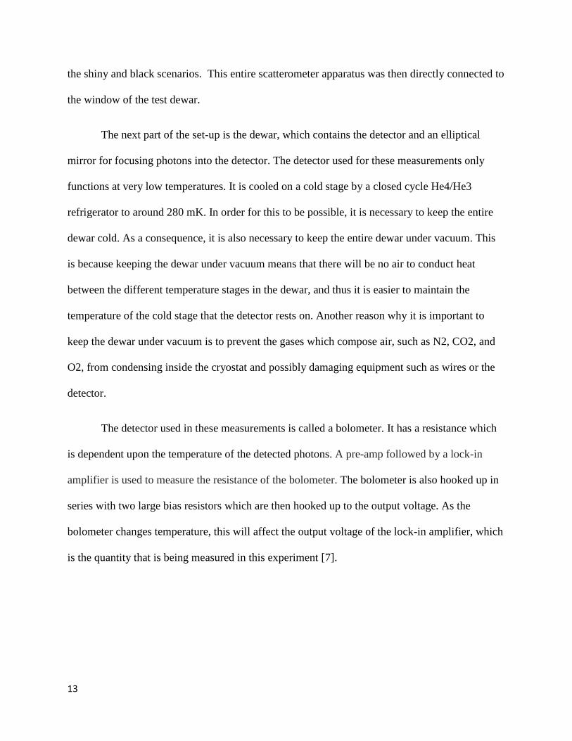
the shiny and black scenarios. This entire scatterometer apparatus was then directly connected to

the window of the test dewar.

The next part of the set-up is the dewar, which contains the detector and an elliptical

mirror for focusing photons into the detector. The detector used for these measurements only

functions at very low temperatures. It is cooled on a cold stage by a closed cycle He4/He3

refrigerator to around 280 mK. In order for this to be possible, it is necessary to keep the entire

dewar cold. As a consequence, it is also necessary to keep the entire dewar under vacuum. This

is because keeping the dewar under vacuum means that there will be no air to conduct heat

between the different temperature stages in the dewar, and thus it is easier to maintain the

temperature of the cold stage that the detector rests on. Another reason why it is important to

keep the dewar under vacuum is to prevent the gases which compose air, such as N2, CO2, and

O2, from condensing inside the cryostat and possibly damaging equipment such as wires or the

detector.

The detector used in these measurements is called a bolometer. It has a resistance which

is dependent upon the temperature of the detected photons. A pre-amp followed by a lock-in

amplifier is used to measure the resistance of the bolometer. The bolometer is also hooked up in

series with two large bias resistors which are then hooked up to the output voltage. As the

bolometer changes temperature, this will affect the output voltage of the lock-in amplifier, which

is the quantity that is being measured in this experiment [7].

14

Figure 4: A diagram of how the bolometer is hooked up to the lock-in amplifier.

15

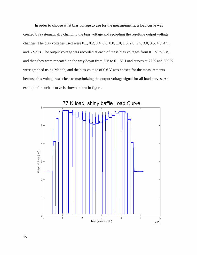
In order to choose what bias voltage to use for the measurements, a load curve was

created by systematically changing the bias voltage and recording the resulting output voltage

changes. The bias voltages used were 0.1, 0.2, 0.4, 0.6, 0.8, 1.0, 1.5, 2.0, 2.5, 3.0, 3.5, 4.0, 4.5,

and 5 Volts. The output voltage was recorded at each of these bias voltages from 0.1 V to 5 V,

and then they were repeated on the way down from 5 V to 0.1 V. Load curves at 77 K and 300 K

were graphed using Matlab, and the bias voltage of 0.6 V was chosen for the measurements

because this voltage was close to maximizing the output voltage signal for all load curves. An

example for such a curve is shown below in figure.

16

Figure 5: Output voltage as a function of bias voltage. Each vertical line marks a change in bias

voltage. The values used for bias voltage increased through 0.1, 0.2, 0.4, 0.6, 0.8, 1.0, 1.5, 2.0,

2.5, 3.0, 3.5, 4.0, 4.5, and 5 Volts, and then decreased back down from 5 V to 0.1 V in these

same step increments.

Methods

Combinations

In order to determine the amount of absorption, scattering, and reflection, it is necessary

to take several different sets of measurements with different combinations of baffle interior,

blackbody load temperature, and the filter in the shelf as well as outside of the shelf. The eight

different combinations of these set-up possibilities are as follows:

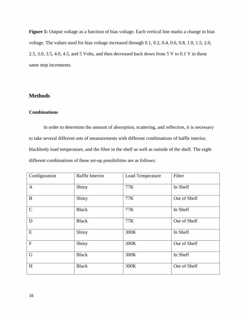
Configuration Baffle Interior Load Temperature Filter

A Shiny 77K In Shelf

B Shiny 77K Out of Shelf

C Black 77K In Shelf

D Black 77K Out of Shelf

E Shiny 300K In Shelf

F Shiny 300K Out of Shelf

G Black 300K In Shelf

H Black 300K Out of Shelf

17

Table 1: A list of each of the combinations used in the set-up. These consist of all the possible

combinations of using either using a black or shiny baffle, a 77K or 300K load, and the filter

being either in or out of the shelf.

For each of these combinations, the final temperature measurement from the detector

depends on the amount of absorption, scattering, reflection, and the fraction of the main beam

that is scattered to the baffle. These properties can be modeled for each combination by adding

the temperature contributions from each of these terms. For example, when the filter is out of the

shelf, the total temperature will have no contribution from the terms involving absorption,

reflection, or scattering, since there is no filter in place to cause these to occur. Thus, the

temperature when the filter is out of the shelf will only depend on how much of the main beam is

spilled over to the baffle. However, when the filter is in the shelf, there will be a term for the

scattering, absorption, and reflection in addition to the spillover to the baffle.

Each configuration shown in the above table will have a different equation relating the

detected temperature to each of the terms for absorption, reflection, scattering, and spillover of

the main beam. This is because the photons interact differently with the set-up depending on the

temperature of the load, the material of the baffle, and whether the filter is in the shelf or not. In

reality, the thermal blackbody load serves as the source for these measurements, and photons are

detected inside of the dewar by the detector. However, it simplifies the problem to work in the

time-reverse case, where the beam is originating from the detector and propagating through the

filter and baffle to the load.

In this time-reversed outlook, when the baffle is shiny, the scattered photons will have the

same temperature as the load because when they hit the side of the baffle, they will be reflected

18

into the load. However, when the baffle is black, the scattered photons will always have a

temperature of 300 K since they will be absorbed in the baffle wall. The absorbed photons will

always have a temperature of 300 K since they are absorbed by the filter, which is at room

temperature (300 K). The reflected photons will always have a temperature that is the same as

the temperature of the dewar, since they are reflected from the filter back into the dewar. Below

is a table of all of the terms that contribute to the final temperature reading for each

configuration. The measured temperature of each configuration is equivalent to the terms in each

row being summed up.

Configuration Main Beam Main Beam

Spillover to Baffle

Absorption Reflection Scattering to

Baffle

A 77*m*(1-a-r-s) 77*(1-m)*(1-a-r-s) 300*a r*Tdewar 77*s

B 77*m 77*(1-m) 0 0 0

C 77*m*(1-a-r-s) 77*(1-m)*(1-a-r-s) 300*a r*Tdewar 300*s

D 77*m 77*(1-m) 0 0 0

E 300*m*(1-a-r-s) 300*(1-m)*(1-a-r-s) 300*a r*Tdewar 300*s

F 300*m 300*(1-m) 0 0 0

G 300*m*(1-a-r-s) 300*(1-m)*(1-a-r-s) 300*a r*Tdewar 300*s

H 300*m 300*(1-m) 0 0 0

Table 2: The temperature contribution of each term to the total (detected) temperature for each

configuration. The configuration labels refer to the combination that they were defined as in

19

Table 1. The terms which contribute to the final temperature are the main beam fraction, the

main beam spillover to the baffle, the absorption, the reflection, and the scattering terms. m, a, r,

and s are the fraction of the incident photons which are in the main beam, absorbed, reflected, or

scattered, respectively. Tdewar is the temperature of the dewar.

Equations Found

In order to get a meaningful relationship between the variables m, a, r, and s, I found the

difference between several of the different combinations (A through H in Tables 1 and 2). The

equations I found relating each of the variables are shown below

r = (F-E) / (300 - Tdewar) [Eq. 1]

a = 1 – r – (E-A) / (F-B) [Eq. 2]

m = 1 – (D-B) / 223 [Eq. 3]

s = (-1 / m) * (((D-C) - (B-A)) / 223 - (1-m)(a+r)) [Eq. 4]

Procedure & Data Analysis

Calibration

Each of the expressions shown in Table 2 has units of temperature. However, the signal

that was read out of the lock-in amplifier had units of voltage. In order to equate the actual

voltage measurements to these equations for the temperature, it was necessary to find a

relationship between the voltage of the lock-in amplifier and the corresponding temperature. In

order to do this, I took several load curves. A load curve is a measurement in which the baffle

20

was shiny, there was no filter in the shelf, the load was a constant temperature, but the bias

voltage was systematically changed and the resulting output voltages were recorded. The bias

voltages used were 0.1, 0.2, 0.4, 0.6, 0.8, 1.0, 1.5, 2.0, 2.5, 3.0, 3.5, 4.0, 4.5, and 5 Volts. The

output voltage was recorded at each of these bias voltages from 0.1 V to 5 V, and then they were

repeated on the way down from 5 V to 0.1 V.

I took a load curve with a 77 K load and another one with a 300 K load (see Figure 5).

Then, since I had chosen to bias all of my measurements at 0.6 V, I took the average of the

voltage during the 0.6 V bias sections for each of the load curves. Then I found the calibration

factor between temperature and voltage by assuming a linear dependence of voltage on

temperature and calculating the ratio C = ΔV/ΔT. ΔT is the difference in temperature between

the two load curves. In this case ΔT = 300 K – 77 K = 223 K. ΔV is the difference in the voltage

that was measured with 0.6 V bias for each of the load curves. In other words, ΔV = V(at 300 K,

bias 0.6 V) – V(at 77 K, bias 0.6 V). Once I found this conversion factor, it was possible to

directly translate the voltage measurements I took into temperatures which I could then equate to

the expressions shown in Table 2.

Temperature of the Dewar

As apparent from the expressions in Table 2, it is necessary to know the temperature of

the dewar in order to find m, a, r, and s. In order to do this, I put an aluminum plate in the shelf.

Since aluminum is completely reflective, all photons detected should have the same temperature

as the dewar. I took four load curves: The first and third load curve was with a 300 K load, shiny

tube, and no device in the shelf. The second and fourth load curves were with the aluminum plate

21

in the shelf. I found the voltage difference at the 0.6 bias voltage between the 300K load and the

aluminum plate. Then, using the known calibration factor of C = ΔV/ΔT, which was described in

the previous section under “Calibration,” I was able to find the temperature of the dewar using

the relation:

C = (V(300 K) – V(Tdewar)) / (300 - Tdewar)

where V(300 K) is the voltage measured at the 0.6 bias voltage for the 300K load curve, and

V(Tdewar) is the voltage measured at the 0.6 bias voltage for the aluminum plate load curve.

After manipulating this equation, one can find:

Tdewar = (V(Tdewar) - V(300 K)) / C + 300

This calculation was done twice, since there were two trials of both the aluminum plate

load curve and the 300 K load curve. These two values were then averaged, and this value was

reported as the temperature of the dewar. The value found was Tdewar = 27 ± 2 K.

Data Analysis for Equations 1 and 4

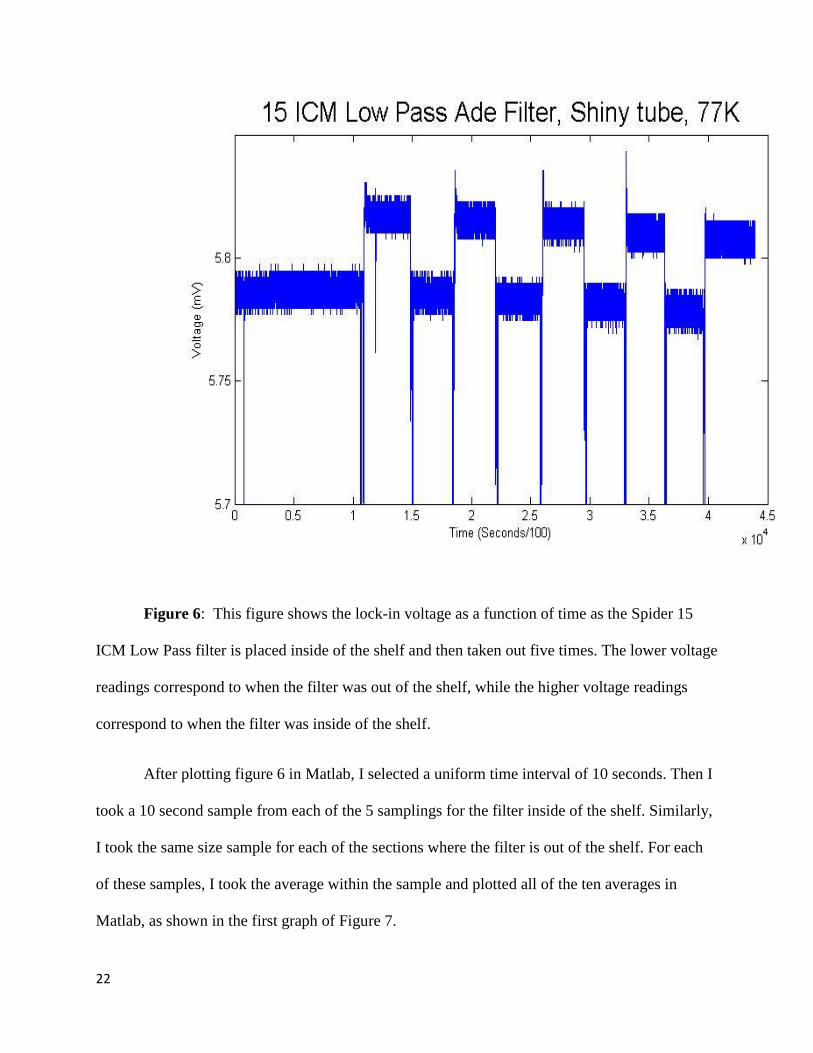
In order to find the quantity (A-B), the shiny baffle, 77 K load was set up. Then the

output voltage was measured as the filter was placed in the shelf and removed five times

consecutively. After taking these measurements, the results were plotted in Matlab, as shown

below. The graph below shows the voltage output as a function of time during this measurement,

for the Spider 15 ICM Low Pass filter.

22

Figure 6: This figure shows the lock-in voltage as a function of time as the Spider 15

ICM Low Pass filter is placed inside of the shelf and then taken out five times. The lower voltage

readings correspond to when the filter was out of the shelf, while the higher voltage readings

correspond to when the filter was inside of the shelf.

After plotting figure 6 in Matlab, I selected a uniform time interval of 10 seconds. Then I

took a 10 second sample from each of the 5 samplings for the filter inside of the shelf. Similarly,

I took the same size sample for each of the sections where the filter is out of the shelf. For each

of these samples, I took the average within the sample and plotted all of the ten averages in

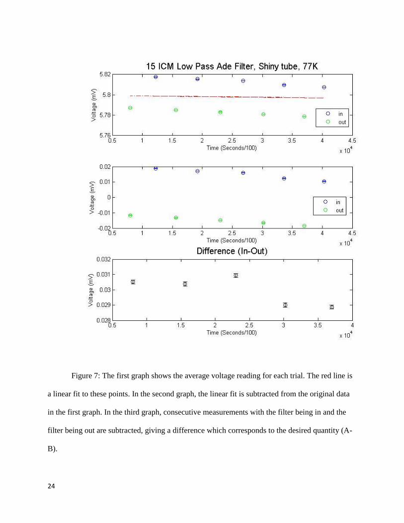
Matlab, as shown in the first graph of Figure 7.

23

Then, as one can see from both Figures 6 and 7, it appears that there is a linear downward

drift in the signal over time. Thus, I performed a linear fit to all of the data in the first graph of

Figure 7, and subtracted this linear fit from the data points. The results are shown in the second

graph of figure 7.

Then, in order to find the desired quantity of (A-B), I found the difference between

consecutive trials of the filter being in the shelf and the filter being out of the shelf. The results of

this calculation are found in the third graph of Figure 7. In order to find one final value for the

quantity (A-B), I found the average of all five of the points. As an error estimate I calculated the

error on the mean among these five points.

24

Figure 7: The first graph shows the average voltage reading for each trial. The red line is

a linear fit to these points. In the second graph, the linear fit is subtracted from the original data

in the first graph. In the third graph, consecutive measurements with the filter being in and the

filter being out are subtracted, giving a difference which corresponds to the desired quantity (A-

B).

25

The same data analysis process was repeated in order to find (D-C), except with a black

baffle and a 77 K load. Similarly, (F-E) was also found using this same process except with a

shiny baffle and a 300 K load. All of these processes and data analysis were repeated using the

Spider 9 ICM Low Pass Ade filter in order to find the analogous quantities of (A-B), (D-C), and

(F-E) for this filter. After finding these values in volts, I used the calibration factor to convert

them into units of temperature.

Data Analysis for Equations 2 and 3

For the combinations shown in Table 1, data was taken by setting up a specific

combination of load temperature and baffle type, but alternating between having the filter in the

shelf and out of the shelf. Thus, data was taken simultaneously for the pairs of combinations (A,

B), (C, D), (E, F), and (G, H). This is why, for Eq. 1 and Eq. 4 it was possible to directly use this

data in order to find (F-E), (D-C), and (A-B). However, for Eq. 2 and Eq. 3, I could not use this

data because measurements were not taken simultaneously for the pairs (A, E), (F, B), or (D, B).

Thus, subtracting these combinations from one another would likely produce inaccurate results

because the data for each configuration was taken so far apart in time that the signal could have

drifted and there would be no way of predicting in which way. In addition, the set-up would most

likely have moved around or changed slightly while the baffle or load was being changed, which

would affect the signal and make it inaccurate to compare measurements taken before and after

the changes.

In order to find the quantity (D-B) for Eq. 3 in a more accurate way, I took four load

curves consecutively: the first and third load curves were taken with a black baffle and a 77 K

load, while the second and fourth load curves were taken with a shiny baffle and a 77 K load. I

26

found the average value of the output voltage at the 0.6 bias voltage points for each load curve.

Then I subtracted the values found for the first two load curves and found an amplitude

corresponding to (D-B). Similarly, I subtracted the values found for the second two load curves

to find another measurement of (D-B). I then averaged these two values and reported that

number as the final result for (D-B).

Chopper Wheel

In order to find the quantity (E-A) / (F-B) without having to subtract non-consecutive

measurements, a chopper wheel was added to the set-up, placed on top of a 77 K nitrogen

blackbody load but below the bottom of the baffle (see Figure 4). The chopper wheel was

divided into four sections. Two of the sections were covered in HR-10 and thus functioned as a

300 K thermal blackbody. The remaining two sections had the inside cut out, and thus the signal

from these sections would simply be that of the 77 K nitrogen blackbody which was stationed

directly below the wheel. Thus, by turning on the chopper wheel, which rotated with a frequency

of approximately 4.35 Hz, the signal output was a sine wave which corresponded to the

amplitude of the change in signal as the wheel chopped between 300 K blackbody and the 77K

nitrogen blackbody load.

27

Figure 4: A diagram of the set-up of the chopper wheel. The wheel was inserted directly

between the 77 K load and the baffle. The chopper wheel was divided into four sections,

alternating between black sections and carved out/empty sections. Thus, as it rotated, the signal

was chopping between that from a 77 K load and that of a 300 K load.

28

Figure 5: A drawing of the chopper wheel. The black sections correspond to sections

covered in HR-10, which function as 300 K blackbodies. The white sections correspond to cut

out sections. Thus, when placed over the 77 K nitrogen load, these sections function as 77 K

blackbodies. The black outline of the wheel is the metal rim which holds the wheel together.

With the chopper wheel continuously running, the filter was put inside of the shelf and

taken out of the shelf five times consecutively. While the filter was inside of the shelf, the

amplitude of the sine wave signal corresponded to a measurement of (E-A). Similarly, when the

filter was not inside of the shelf, the amplitude of the sine wave signal corresponded to a

measurement of (F-B). By taking the ratio of each consecutive in/out measurement, it was

29

possible to obtain a value for (E-A) / (F-B), which was the necessary quantity to measure for

subbing into Eq. 2.

Results

After doing the data analysis described in the previous section, I found the following

results for the Spider 9 ICM Low Pass filter:

Quantity Value Error

F-E 3.24 0.04

(E-A) / (F-B) 1.02 0.03

D-B -0.05 0.02

(D-C) - (B-A) -0.8 0.1

Table 3: Results found for the unknown quantities in equations 1-4 for the Spider 9 ICM Low

Pass filter. All units are in Kelvin.

For the Spider 15 ICM Low Pass filter I found the following results:

Quantity Value Error

F-E 14.5 0.2

(E-A) / (F-B) 1.01 0.05

D-B -0.05 -0.02

30

(D-C) - (B-A) -3.46 0.06

Table 4: Results found for the unknown quantities in equations 1-4 for the Spider 15 ICM Low

Pass filter.

The values found for each of the quantities in Table 3 can be directly substituted into

Equations 1, 2, 3, and 4 in order to find the fraction of incident photons which were absorbed (a),

reflected (r), scattered to the baffle (s), and remained in the main beam (m). Final results

indicated the following values for the Spider 9 ICM Low Pass filter:

Quantity Value Error

r 0.0118 0.0007

a -0.03 0.03

m 1.00 7*10^-5

s 0.0037 0.0006

Table 5: The results for r, a, m, and s for the Spider 9 ICM Low Pass filter. The quantities r, a,

m, and s represent the fraction of incident 150 GHz photons which were reflected, absorbed,

stayed in the main beam, and were scattered to the baffle, respectively.

The final results for reflection, absorption, main beam fraction, and scattering to the

baffle for the 15 ICM Low Pass filter were found by the same method of directly substituting the

values from table 4 into equations 1 through 4 for a, r, s, and m. The results are as follows:

31

Quantity Value Error

r 0.053 0.003

a -0.07 0.05

m 1.00021 7.83*10^-5

s 0.0155 0.0003

Table 6: The results for r, a, m, and s for the Spider 15 ICM Low Pass filter. The quantities r, a,

m, and s represent the fraction of incident 150 GHz photons which were reflected, absorbed,

stayed in the main beam, and were scattered to the baffle, respectively.

Conclusion

This project proved that it is possible to measure absorption, scattering, and reflection

properties for optical devices using a scatterometer and a thermal blackbody load. In addition, it

set limits on the amount of absorption, scattering, and reflection that are caused by the two

Spider low pass filters that were tested during this project. One area of concern in the results of

this experiment is the negative values found for the absorption fraction. Although these values

were mostly within the error estimates of zero, it is still a point of concern that the error was so

high. If this experiment is to be repeated in the future, it would be useful to improve the

absorption measurements.

32

Sources

[1] A.A. Penzias and R.W. Wilson. A Measurement of Excess Antenna Temperature at 4080

Mc/s. Atrophys. J., 142:419-421, July 1965.

[2] Smoot, G.F. et al. “Structure in the COBE DMR First Year Maps”. 1992, ApJ, 396, L1.

[3] C. L. Bennett, et. al. “First-Year Wilkinson Microwave Anisotropy Probe (WMAP)

Observations: Preliminary Maps and Basic Results”. 148:1-27, Setpember 2003. astro-

ph/0302207.

[4] W. C. Jones, et. al. “A measurement of the angular power spectrum of the CMB temperature

anisotropy from the 2003 flight of Boomerang”. The Astrophysics Journal , 647:823-832, 1006.

[5] J. Nagy, Personal Communication. 29 October 2013.

[6] J. Filippini, L. Moncelsi, B. Tucker, Personal Communication. 11 November 2013.

[7] M. Runyan. “A Search for Galaxy Clusters Using the Sunyaev-Zel’dovich Effect.” 20

December 2002.