NBER WORKING PAPER SERIES

MEASURING DISCRIMINATION IN EDUCATION

Rema HannaLeigh Linden

Working Paper 15057http://www.nber.org/papers/w15057

NATIONAL BUREAU OF ECONOMIC RESEARCH1050 Massachusetts Avenue

Cambridge, MA 02138June 2009

¸˛This project was funded in part by University Research Challenge Fund at New York University.We thank Payal Hathi for outstanding research assistance. We thank Abhijit Banerjee, Asim Khwaja,Sendhil Mullainathan, Rohini Pande, and Jonah Rockoff for helpful comments. The views expressedherein are those of the author(s) and do not necessarily reflect the views of the National Bureau ofEconomic Research.

NBER working papers are circulated for discussion and comment purposes. They have not been peer-reviewed or been subject to the review by the NBER Board of Directors that accompanies officialNBER publications.

© 2009 by Rema Hanna and Leigh Linden. All rights reserved. Short sections of text, not to exceedtwo paragraphs, may be quoted without explicit permission provided that full credit, including © notice,is given to the source.

Measuring Discrimination in EducationRema Hanna and Leigh LindenNBER Working Paper No. 15057June 2009JEL No. I2,J16

ABSTRACT

In this paper, we illustrate a methodology to measure discrimination in educational contexts. In India,we ran an exam competition through which children compete for a large financial prize. We recruitedteachers to grade the exams. We then randomly assigned child “characteristics” (age, gender, and caste)to the cover sheets of the exams to ensure that there is no systematic relationship between the characteristicsobserved by the teachers and the quality of the exams. We find that teachers give exams that are assignedto be lower caste scores that are about 0.03 to 0.09 standard deviations lower than exams that are assignedto be high caste. The effect is small relative to the real differences in scores between the high andlower caste children. Low-performing, low caste children and top-performing females tend to loseout the most due to discrimination. Interestingly, we find that the discrimination against low castestudents is driven by low caste teachers, while teachers who belong to higher caste groups do not appearto discriminate at all. This result runs counter to the previous literature, which tends to find that individualsdiscriminate in favor of members of their own groups.

Rema HannaKennedy School of GovernmentHarvard University79 JFK StreetCambridge, MA 02138and NBERrema_hanna@ksg.harvard.edu

Leigh Linden1306 International Affairs Building420 West 118th Street, Mail Code 3323New York, NY 10027ll2240@columbia.edu

1

I. Introduction

Teachers’ expectations seem to affect students’ behavior. Numerous studies have documented

what is known as the Pygmalion effect, through which students perform better (or worse) simply

because they are expected to do so. For example, the seminal paper in the literature, Rosenthal

and Jacobson (1968), has shown that individual students outperformed other students in school

after their teachers were told at the start of the school year that they had excelled on a

standardized test (even though they were randomly picked as “excelling”). Although this effect

has been well documented, we do not yet understand the factors that teachers use to formulate

prior opinions about students’ abilities. Of particular concern is whether or not teachers base

their beliefs on students’ affiliations with a minority group. If this type of discrimination does

exist, it can have long lasting effects, both reinforcing erroneous beliefs of inferiority (Steele and

Aronson 1995, 1998; Hoff and Pandey, 2006) and discouraging children from making human

capital investments (Mechtenberg, 2008; Taijel, 1970; Arrow 1972; Coate and Loury, 1993).

Discrimination would, thus, hinder the effectiveness of education in leveling the playing field

across children from different backgrounds.

Unfortunately, it is difficult to empirically test whether discrimination exists in the

classroom. By definition, children from disadvantaged backgrounds exhibit many characteristics

that are associated with poor academic performance—few educational resources in schools, low

levels of parental education, families with little human or social capital, and even high rates of

child labor. Thus, it is hard to understand whether children who belong to these minority groups

perform worse in school, on average, due to discrimination or due to these other characteristics

that may be associated with a disadvantaged background. Moreover, as Anderson, Fryer and

Holt (2006) discuss, “uncovering mechanisms behind discrimination is difficult because the

2

attitudes about race, gender, and other characteristics that serve as a basis for differential

treatment are not easily observed or measured.”

We address this question through an experiment built around a prize exam competition.

The method we illustrate can be used to measure discrimination in many educational contexts

and locations; however, we demonstrate it in the Indian context, where discrimination based on

caste is a potentially serious problem. Specifically, we designed an exam competition in which

we recruited children to compete for a large financial prize. We, then, recruited local teachers

and provided each teacher with a set of exams. We randomly assigned child “characteristics”

(age, gender, and caste) to the cover sheets of the individual exams graded by the teachers to

ensure that there would be no systematic relationship between the characteristics observed by the

teachers and the quality of the exams.

This design has several key advantages. First, the random assignment allows us to

overcome one of the major obstacles in measuring discrimination. Specifically, we can attribute

any differences in the exam scores across different types of children to discrimination and not to

other characteristics associated with belonging to a disadvantaged group. Second, the richness of

the data available in the experiment allows us to investigate the structure of the observed

discrimination and to understand how teachers discriminate, when they discriminate, and against

which types of students.

Within the education literature, our work is closely related to a rich body of work in the

United States that uses laboratory experiments to evaluate teachers’ perceptions of African

American students relative to Caucasian students. While the employed techniques range from

evaluations of actual tests to video tapes of student performance and to measurements of teachers

reactions to different students (see Furgeson (2003) for a thorough literature review), the basic

3

strategy is to hold students’ performance constant while varying the race of the student so that

any variation in the experimental subjects’ reaction to the student is due only to the students’

race. Most of these studies find evidence of lower expectations of the performance of African

American students and evidence of discrimination in evaluations. Our work is also very much

also related to Lavy (2004), which uses a natural experiment to measure discrimination in

grading by gender in Israel.

However, our methods are most analogous to the types of field experiments that have

been used to measure racial discrimination in labor market settings. These experiments typically

measure discrimination in the hiring of actual applicants. The researchers either have actual

individuals apply for jobs (Fix and Struyk, 1994) or they may submit fictitious job applications

to actual job openings (Bertrand and Mullainathan, 2004; Banerjee, Bertrand, Mullainathan, and

Datta, 2009; Siddique, 2008); in both cases, the “applicants” are statistically identical in all

respects, except for race or caste group. Unlike pure laboratory experiments, in which

individuals are asked to perform assessments in a consequence-less environment, a major

advantage of these experiments is that they are able to measure the behavior of actual employers

making real employment decisions.

In our study, we break the correlation between observed characteristics and student

quality by randomly assigning characteristics to an exam cover sheet before it is graded. We

then place teachers in an environment in which their behavior affects the wellbeing of the child,

In particular, teachers know that the results of their grading will result in a substantial prize to the

winning child (58 USD or 55.5 percent of the parents’ monthly income). Thus, we are able to

mimic the incentives faced by teachers in the classroom.

4

We find evidence of discrimination against lower caste children. Specifically, we find

that teachers give exams that are assigned to be “lower caste” scores that are about 0.03 to 0.09

standard deviations lower than those that are assigned to be “high caste.” We do not find any

overall evidence of discrimination by gender or age. Disaggregating the results by the quality of

the exam, the low-performing, low caste children and top-performing females tend to lose out the

most due to discrimination. Interestingly, we find that the discrimination against low caste

children is driven by low caste teachers, while teachers from the high caste groups do not appear

to discriminate at all. Finally, we find that teachers tend to discriminate more towards children

who are graded early in the evaluation process, suggesting that teachers use demographic

characteristics to help grade when they are not yet confident with a testing instrument.

The rest of the paper proceeds as follows. Section II provides some background on caste

discrimination and education in India. Section III describes the methodology, while Section IV

describes our data. Our findings are presented in Section V. Section VI provides a discussion of

the key results, while Section VII concludes.

II. Background

In India, individuals in the majority Hindu religion were traditionally divided into hereditary

caste groups that denoted both a family’s place within the social hierarchy and their professional

occupation. In order of prestige, these castes were the Brahmin, Kshatriya, Vaishya, and Shudra

denoting respectively, priests, warriors/nobility, traders/farmers, and manual laborers. Within

each main caste, many subcastes exist that also have varying levels of prestige.

In principle, individuals are now free to choose occupations regardless of caste, but like

race in the United States, the historical distinctions have created inequities that still exert

5

powerful social and economic influence.1

In this section, we first describe the methodology that we designed to understand whether

discrimination exists in grading. We then discuss the data and lay out our empirical

methodology.

Given the large gap in family income and labor

market opportunities between children from lower and high caste groups, it is not that

unsurprising that children from traditionally more disadvantaged caste groups tend to have worse

educational outcomes than those from the more advantaged groups. For example, Bertrand,

Hanna, and Mullainathan (2008) show large differences in entrance exam scores across caste

groups entering engineering colleges, while Holla (2008) shows similar differences in final high

school exams.

While it is difficult to identify the influence of caste separately from poverty and low

socio-economic status, the potential for discrimination in schools is significant. Both urban and

rural schools maintain detailed records of their students’ caste and religion, along with other

demographic information such as their age, gender, and various information on their parents (see,

for example, He, Linden, and MacLeod, 2008). Anecdotal evidence suggests that teachers may

take this information into account. For example, the Probe Report of India (1999) cites cases of

teachers banning lower caste students from joining school. Shastry and Linden (2008) show that

caste is correlated with the degree to which teachers are willing to exaggerate the attendance of

students enrolled in an educational program that provides grain to high attending students.

III. Methodology

1 Banerjee and Knight (1985); Lakshmanasamy and Madheswaran (1995); Unni (2002) give evidence of inequality across groups by earnings, while Rao (1992), Chandra (1997), and Munshi and Rosenzweig (2005) show evidence of inequality in social and economic mobility. Deshpande and Newman (2007) and Madeshwaran and Attewell (2007) provide some evidence of discrimination in earnings, while Siddique (2008) and Jodhka and Newman (2007) for discrimination in hiring practices.

6

A. Research Design

We designed an experiment that comprises of three components: child testing sessions, the

creation of grading packets, and teacher grading sessions. We first recruited children to

participate in a prized exam competition. After the competition, we copied the tests that the

children completed and compiled them into grading packets. Each test copy in the grading

packet was assigned an information sheet that included randomly assigned demographic

characteristics. We then recruited local teachers to participate in a grading session, during which

the teachers graded the exams that displayed the randomly assigned characteristics.

Child Testing Sessions

In April 2007, we ran exam tournaments for children aged seven to fourteen years of age. Our

project team went door to door to invite parents to allow their children to attend a testing session

to compete for a Rs 2500 prize (about $US 58).2

Over a two week period, sixty-eight children attended four testing sessions. The testing

sessions were held in various places, such as community halls, empty homes, or temples,

The project team informed the families that

prizes would be distributed to the highest scoring child in each of the two age groups (7 to 10

years of age, and 11 to 14 years of age), that the exams would be graded by local teachers after

the testing sessions, and that the prize would be distributed after the grading was complete. The

prize is a significant sum of money, given that the parents reported earning an average of 4,500

Rs per month ($US 104) in the parent survey that we administered.

2 For recruitment, our project team mapped the city: they collected demographic information about each community and also identified community leaders who they might be able to work with later in the project. To ensure that children of varying castes would be present at each session, the team tried to either recruit from neighborhoods where the children were of diverse caste groups or to recruit from several uniform caste neighborhoods.

7

centrally located to the communities from which the children were selected. They were held on

weekends to ensure that they did not conflict with the school day and that parents would be able

to accompany the children to the sessions. During the testing sessions, the survey team first

obtained informed consent from the parents for both their participation in the parent survey and

their child’s participation in the tournament. Next, the survey team administered a short survey

to the children’s parents to collect information on the child (gender, age) and to also collect basic

demographic characteristics of the family (income background, employment status of the father,

and caste information).

After the survey, the project team obtained written assent from each participating child

and began the actual exam. To vary the subjectivity of the exam questions, we included

questions that tested the basic math and language skills contained in the standard Indian

curriculum, as well as an art section in which the children were asked to display their creativity.

The exam took approximately 1.5 hours. All children who participated in the testing session

received a reading workbook at the time of the sessions and were told that they would be

contacted with information about the prize when grading was complete.

Randomizing Child Characteristics

The key to our experimental design is to break the correlation between the children’s actual

performance on an exam and the child characteristics perceived by the teacher when grading the

exam. In a typical classroom setting, one can only access data on the actual grades teachers

assign to students whose characteristics the teachers know. This makes it impossible to identify

what grade the teacher would have assigned had another child, with different socio-economic

characteristics, completed the exam in an identical manner. Our experimental design allows us

8

to ensure the independence of the exams’ quality and the characteristics observed by the

teachers.

Specifically, we randomized the demographic characteristics observed by teachers on

each exam. Each teacher was asked to grade a packet containing 25 exams. To form these

packets, each test completed by a student was stripped of identifying information, assigned an ID

number, and photocopied. Twenty-five copies were then randomly selected to form each packet,

without replacement, to ensure that the same teacher did not grade the same photocopied test

more than once. Each exam in the packet was then assigned a socio-demographic coversheet,

which contained the basic demographic information for the “child.” This included a child’s first

name, last name, gender, caste information, and age.3 However, these child characteristics were

randomly assigned from the characteristics of children sitting for the exams. By teacher, we

stratified the assignment of the characteristics to ensure that each teacher observed coversheets

with the same proportion of characteristics of each type of child, avoiding the possibility that a

teacher was assigned to grade children of a single sex or caste. Since most Indian first names are

gender specific, the first name and gender were always randomized together. Similarly, many

last names are also caste specific and, therefore, we randomized the last name and the caste

together.4

Caste, age, and gender were each drawn from an independent distribution. We randomly

selected the ages of the students from a uniform distribution between eight and fourteen. We

ensured that gender was equally distributed among the males and females. Caste was assigned

For each teacher, we sampled the name of the child without replacement so that the

teacher would not be grading two different exams from the same child.

3 We also include caste categories (General, Other Backward Caste, Scheduled Caste, and Scheduled Tribe), which are groupings of the caste categories. 4 While this strategy has the advantage of consistently conveying the caste information to teachers, it does prevent us from identifying the specific channel through which teachers are getting the information. It may be possible, for example, that the name alone is enough to convey the caste of the child.

9

according to the following distribution. Twelve and a half percent of the exams were assigned

each to the highest caste (Brahmin) and the next caste (Kshatriya). Fifty percent of the exams

were assigned to the Vaishya Caste and twenty-five percent were assigned to the Shudra Caste.5

The recruitment proceeded as follows. First, the project team talked with the headmaster

of the school to obtain permission to recruit teachers from the school. Once permission was

obtained, the project team explained to the teachers that they would like to invite them to

participate in a study to understand grading practices. The teachers were told that they would

grade the exams of twenty-five children and that they would be compensated for their work with

a Rs 250 (about $US 5.80) payment. The project team also informed the teachers that the child

who obtained the highest score based on the grading would receive a prize worth Rs 2500 (about

Each exam was graded by an average of forty-three teachers. Since the “observed”

characteristics of the child were randomly assigned, we would expect that these characteristics

would be uncorrelated with the exam grade in a world with no discrimination. Any correlation

between the “observed” characteristics and exam scores is, thus, evidence of discrimination.

Teacher Grading Sessions

After creating the packets, we recruited teachers to grade the exams. We obtained a listing of

schools in the city from the local government, and we divided the schools into government and

private schools. For each category, we ranked the schools using a random number generator.

The project team began recruitment at the schools at the top of the list, and went down the list

until they obtained the desired number of teachers. In total, the project team visited about 167

schools to recruit 120 teachers, 67 from government schools and 53 from private schools.

5 The purpose of this distribution was originally to ensure variation in both caste and the caste categories to which children could be assigned. These classifications are restricted to the lowest two classes and ensure equal distribution among each category, resulting in 75 percent of the exams being assigned to these castes.

10

$US 58). This prize was designed to establish incentives for the teachers’ grading by ensuring

that the grades received on the exam have real effects on the well-being of the children, thereby

mimicking the incentives faced by teachers in school.

On average, a grading session lasted about two hours for each teacher. At the sessions,

the project team first obtained consent. Next, the project team provided the teachers with a

complete set of answers for the math and language sections of the test, and the point system per

question for all three sections of the test. The project team went through the answer set question

by question with the teachers. Teachers were told that partial credit was allowed, but the project

team did not describe how partial credit should be allocated. Thus, the teachers had the

discretion to allocate partial credit points as they felt appropriate.

Next, the grading portion of the session began. The teacher received twenty-five

randomly selected exams—with the randomly assigned cover sheets—to grade as well as a

“testing roster” to fill out. To ensure that teachers viewed the demographic information, we

asked them to copy the information from the cover sheet onto the grade roster. They were then

asked to grade the exam and input the total score and the individual grades for each section of the

exam—math, language, and art—onto the testing roster.

When a teacher finished grading his or her packet of exams, the project team

administered a short survey to the teacher. The survey consisted of questions designed to gauge

the demographic characteristics and teaching philosophy of each teacher.

11

After all the grading sessions were complete, we computed the average grade for each

child across all teachers who graded his or her exam. We then awarded the prize to the highest

scoring child in each of the age categories, based on these average grades.6

6As the tests were equally likely to be assigned the characteristics described any negative (or positive effects) received from being assigned particular characteristics should be equal across individual tests, making the overall average a fair assessment of student performance.

B. Data Description

We compiled three sets of data: exam scores, parent surveys, and teacher surveys. We collected

two sets of exam scores. The first set includes the test scores generated by each teacher. In

addition, a member of the research staff graded each exam using the same grading procedures as

the teacher, but on a “blind” basis in which they had no access to the original characteristics of

the students taking the exam or any assigned characteristics. This was done to provide an

“objective” assessment of the quality of the individual exam. The set of exam scores includes

the total score and a score on each subject (math, hindi, and art).

Each subject was chosen to provide variation in the objectivity with which the individual

sections could be evaluated. Math was chosen to be the most objective section and questions

covered counting, greater than/less than, number sequences, addition, subtraction, basic

multiplication, basic addition, and simple word problems among a few other basic competencies.

Language, which was chosen to be the intermediately objective section, included questions

covering basic vocabulary, spelling, synonyms, antonyms, and basic reading comprehension, and

so forth. Finally, the art section was designed to be the most subjective. In this section, we

asked the children to draw a picture of their family doing their favorite activity and then to

explain the activity.

12

We normalized the exam scores of each section and the overall total scores in the analysis

that follows, to facilitate comparisons with other studies in the literature. To do so, we pool all

of the grades assigned to each test copy by the teachers, and for each exam, subtract the overall

mean and divide by the standard deviation of the scores. Each section and the overall exam

score are normalized relative to the distribution of the individual scores for the respective

measure.7

The random assignment of tests to teachers and children’s characteristics to the coversheets

should ensure that there is no systematic correlation between the quality of the graded tests, the

In addition to the test data, we have data from the two surveys we administered. First, we

have data from a survey of the children’s parents that was conducted in order to collect

information on the socio-demographic background of the children. Most importantly for the

experiment, this included information on the family’s caste, the age of the child, and the child’s

gender. Second, we have data from the teacher survey, which included basic demographic

information as well as questions regarding the types of students that the teachers normally teach.

The demographic information included the teachers’ religion, caste, the type of school at which

they taught (public or private), their educational background, age, and gender. In addition, we

also collected information on the characteristics of teachers’ students. Note that there was

almost no variation in teachers’ responses to these questions – all of the teachers taught low

income students like those in our sample, either in a local public or private school.

C. Empirical Strategy

7 In results not presented in this draft, we have also estimated the results normalizing relative to the distribution of blind test scores. Since this is a linear transformation of the dependent variable, it does not affect the hypothesis tests, nor does it affect the magnitude of the estimated results.

13

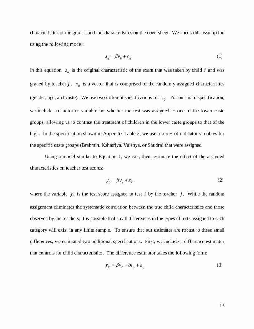
characteristics of the grader, and the characteristics on the coversheet. We check this assumption

using the following model:

ijijij vz εβ += (1)

In this equation, ijz is the original characteristic of the exam that was taken by child i and was

graded by teacher j . ijv is a vector that is comprised of the randomly assigned characteristics

(gender, age, and caste). We use two different specifications for ijv . For our main specification,

we include an indicator variable for whether the test was assigned to one of the lower caste

groups, allowing us to contrast the treatment of children in the lower caste groups to that of the

high. In the specification shown in Appendix Table 2, we use a series of indicator variables for

the specific caste groups (Brahmin, Kshatriya, Vaishya, or Shudra) that were assigned.

Using a model similar to Equation 1, we can, then, estimate the effect of the assigned

characteristics on teacher test scores:

ijijij vy εβ += (2)

where the variable ijy is the test score assigned to test i by the teacher j . While the random

assignment eliminates the systematic correlation between the true child characteristics and those

observed by the teachers, it is possible that small differences in the types of tests assigned to each

category will exist in any finite sample. To ensure that our estimates are robust to these small

differences, we estimated two additional specifications. First, we include a difference estimator

that controls for child characteristics. The difference estimator takes the following form:

ijijijij zvy εδβ ++= (3)

14

The vector of randomly assigned characteristics is given by ijv as in equation (1), and ijz is a

linear control function that includes the true characteristics of the child taking test i . Second, we

include a fixed-effects estimator, which takes the following form:

ijjjijijij wzvy ετδβ +++= (4)

where jw is the grader fixed effects. This specification allows us to control for fixed differences

in grading practices across teachers.

IV. DESCRIPTIVE STATISTICS AND INTERNAL VALIDITY

In this section, we first provide descriptive statistics on the characteristics of the children who sat

for the exam and the teachers who graded it. Next, we explore whether the original

characteristics of the child predicts the exam score. Finally, we provide a check on the

randomization.

A. Baseline Data

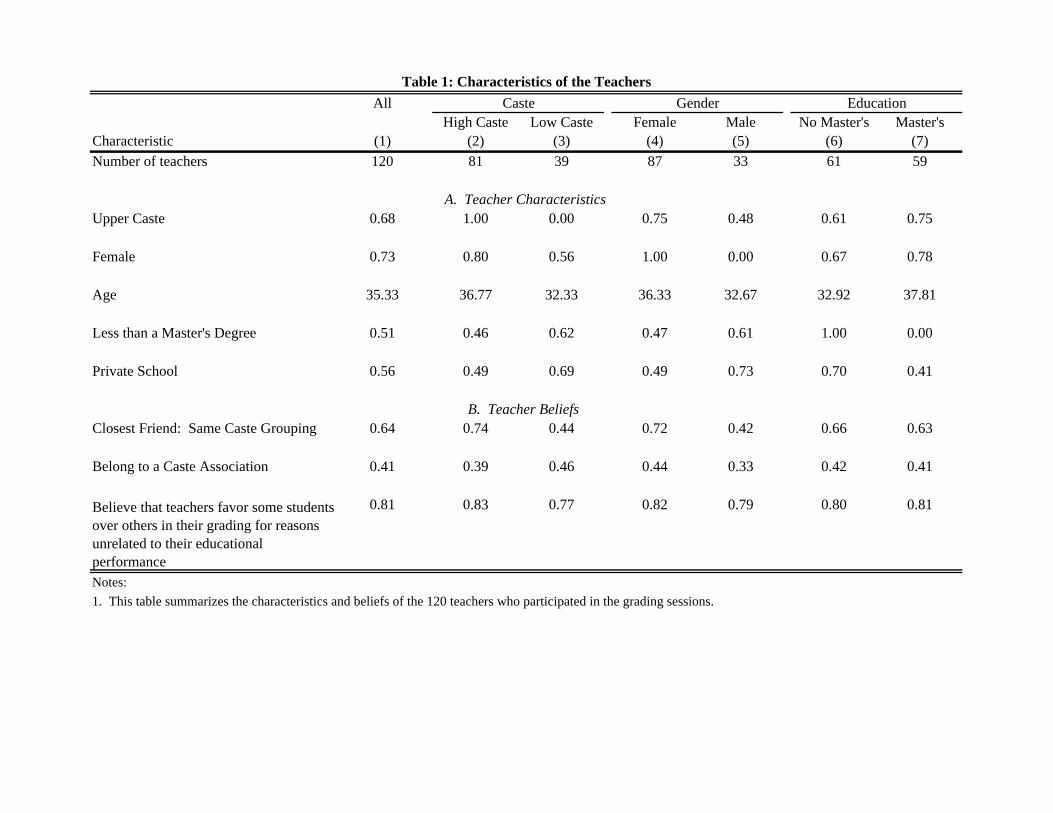
In Table 1, we provide descriptive statistics on the 120 teachers who participated in the exam

competition. Panel A provides information on the demographic characteristics of the teachers,

while Panel B provides sample statistics on their caste identity and beliefs. In Column 1, we

provide the summary statistics for the full sample. In the subsequent columns, we disaggregate

the data by their basic demographic characteristics: in Columns 2 and 3, we divide the sample

by the teachers’ caste. In Columns 4 and 5, we disaggregate the sample by the teachers’ gender,

and finally, we divide the sample by the teachers’ education level in Columns 6 and 7.

Reflecting the fact that teaching (especially at a public school) is a well-paid and

desirable occupation, sixty-eight percent of the teachers identify themselves as belonging to the

15

upper caste groups (Panel A, Column 1). Teachers tend to be relatively young (an average age

of thirty five) and female (seventy-three percent). We made a point to recruit at both public and

private schools. The effort was successful in that we recruited a fairly equal number of teachers

across the two groups into the sample. Forty-four percent of the teachers work in public schools,

while fifty-six percent work in private schools. About half the sample holds a master’s degree.

As Panel B demonstrates, caste identity is high among the teachers. Sixty-four percent

report that their closest friend is of the same caste grouping and forty-one percent report that they

belong to a caste association. Interestingly, even the teachers themselves tend to report that they

believe that “teachers favor some students over others in their grading for reasons unrelated to

educational performance.” Eighty-one percent of the teachers agreed with this statement.

Comparing the characteristics of teachers across Columns 2 through 7, the relationships

between the various characteristics generally follows the expected patterns. Low caste teachers

are more represented in the comparatively less desirable private school teaching positions, less

likely to have a master’s degree, more likely to be male, and more likely to belong to a caste

association (Columns 2 – 3). Female teachers tend to belong to the high caste groups (75 percent

for versus 48 percent for men) and are also more likely to have a master’s degree (Columns 4 –

5). The somewhat surprising pattern lies in the relationship between education and beliefs (Panel

B, Columns 6 – 7). We do not observe a difference in caste identity or beliefs across those with

and without a master’s degree.

In Table 2, we provide summary statistics for the children who participated in the exam

competition and the characteristics observed by the teachers. We describe the original

characteristics of the children and the characteristics of the children observed by the teacher in

Columns 1 and 2, respectively. Column 1 contains averages for the actual sixty-nine children,

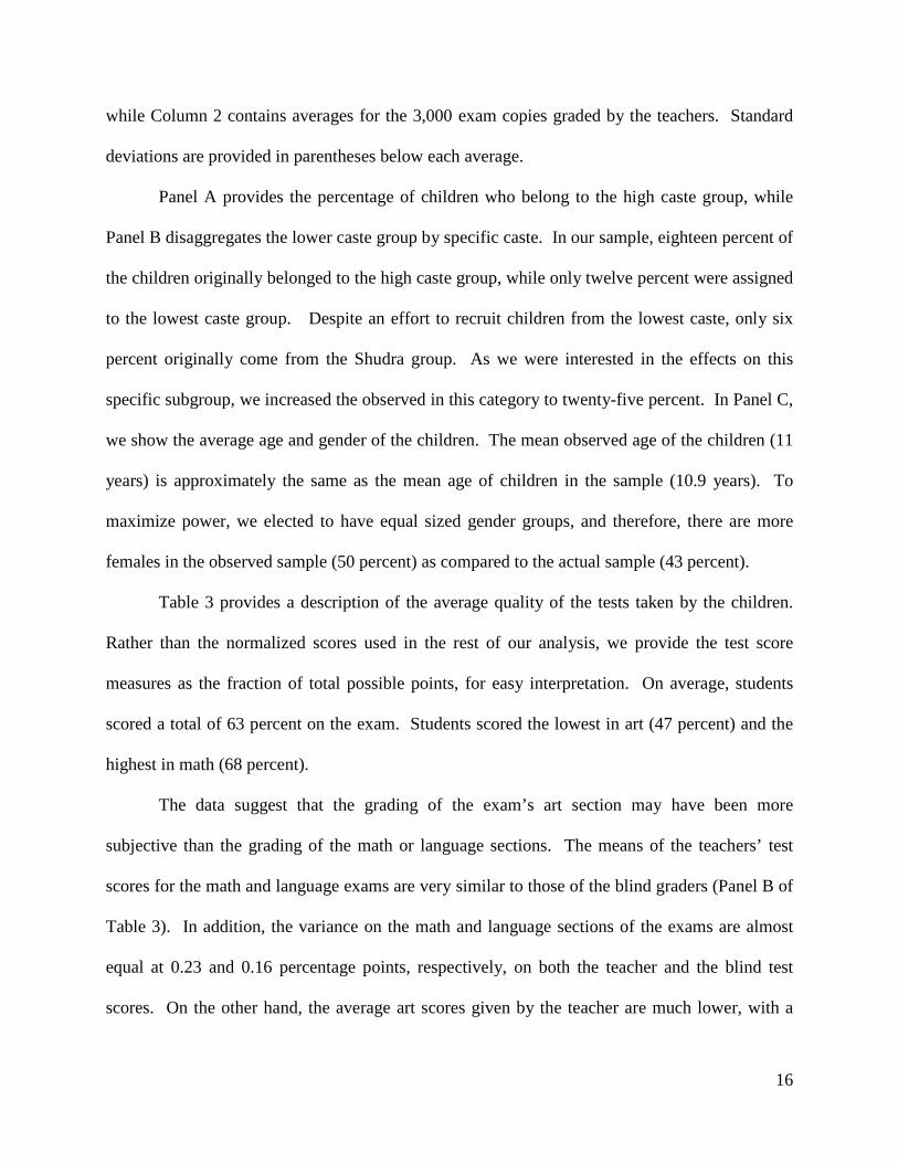
16

while Column 2 contains averages for the 3,000 exam copies graded by the teachers. Standard

deviations are provided in parentheses below each average.

Panel A provides the percentage of children who belong to the high caste group, while

Panel B disaggregates the lower caste group by specific caste. In our sample, eighteen percent of

the children originally belonged to the high caste group, while only twelve percent were assigned

to the lowest caste group. Despite an effort to recruit children from the lowest caste, only six

percent originally come from the Shudra group. As we were interested in the effects on this

specific subgroup, we increased the observed in this category to twenty-five percent. In Panel C,

we show the average age and gender of the children. The mean observed age of the children (11

years) is approximately the same as the mean age of children in the sample (10.9 years). To

maximize power, we elected to have equal sized gender groups, and therefore, there are more

females in the observed sample (50 percent) as compared to the actual sample (43 percent).

Table 3 provides a description of the average quality of the tests taken by the children.

Rather than the normalized scores used in the rest of our analysis, we provide the test score

measures as the fraction of total possible points, for easy interpretation. On average, students

scored a total of 63 percent on the exam. Students scored the lowest in art (47 percent) and the

highest in math (68 percent).

The data suggest that the grading of the exam’s art section may have been more

subjective than the grading of the math or language sections. The means of the teachers’ test

scores for the math and language exams are very similar to those of the blind graders (Panel B of

Table 3). In addition, the variance on the math and language sections of the exams are almost

equal at 0.23 and 0.16 percentage points, respectively, on both the teacher and the blind test

scores. On the other hand, the average art scores given by the teacher are much lower, with a

17

mean of 47 percent for the teachers compared with 64 percent for the blind graders. Moreover,

the larger variance for the art section (0.32) provides confirming evidence that, as intended, the

art section may have been more subjective than the other sections of the exam.

Moving away from the differences in subjectivity across tests, the data indicate that

regardless of the subject, teachers do exhibit a fair amount of discretion in grading overall.

Figure 1 provides a description of the total test score range (in percentages) per test. The score

ranges per exam are quite large, particularly at the lower portion of the test quality distribution.

This indicates that the teachers assign partial credit very differently.

Who won the exam competition? In reality, low caste females won both age categories.

The two winning exams each displayed the low caste characteristics about 80 percent of the time.

About half the time, the winning exams were assigned as female and the average age on the

winning exams was eleven years old. Thus, the winning exam was, on average, assigned the

mean characteristics in our sample, as we would predict given the randomization.

B. Do Actual Characteristics Predict Exam Scores?

We next investigate the relationship between the actual characteristics of the children in our

sample and their exam scores. In the first column of Table 4, we present the simple correlation

between the total test scores that the teachers assigned to the exams and the true underlying

characteristics of the children. In Column 2, we add the blind test score as an additional control.

In Columns 3 -5, we disaggregate the test scores by individual subjects. All scores have been

normalized relative to the overall distribution of scores for each respective section.

The children’s original demographic characteristics strongly predict the exam scores.

Children from the lower caste group score about 0.41 standard deviations worse on the exam

18

than the high caste group (Column 1).8

8Appendix Table 1 replicates the table including disaggregated caste groups. Recall that the caste groups in terms of descending order of prestige are the Brahmin, Kshatriya, Vaishya, and Shudra castes. Children who belong to Kshatriya caste perform worse (-0.17 standard deviations) than the students who belong to Brahman caste, which is the omitted category in the regressions (Column 1). Children from the Vaishya caste then score worse than the students from the Kshatriya caste by 0.35 standard deviations, and children who belong to the Shudra group score the worst (-1.17 standard deviations lower than the children from the Brahman caste).

Females, on average, score 0.18 standard deviations

higher on the exam than males. Finally, one additional year of age is associated with an

additional 0.85 standard deviations in score, although this effect is declining with years of age.

In Column 2, we replicate the specification in Column 1, adding the score that our blind

grader awarded to each exam as an additional control variable. The blind score provides us with

a measure of performance on the exam that reflects only the underlying quality of the exam.

Any difference between the test scores from the teachers and the scores from the blind grading

can be attributed partially to discrimination, but also to the natural variation in grading practices.

The total blind score awarded to the test is highly correlated with the score that the teachers

assigned to the tests. On average, a one standard deviation increase in the blind scores results in

a 0.93 standard deviations increase in the total test score. When we include the blind test score,

the coefficients on the low caste and female indicator variables more closer to zero, but the age

variable still is a significant predictor of the final score.

We, next, disaggregate the test score data by subject in Columns 3 – 5 of Table 4. The

results suggest that the different sections of the exam do provide variation in subjectivity, with

the art section being much more subjective than the other sections. The correlation between the

blind score and the teacher’s score for the math and language sections is the same as for the

overall score (about 0.93). The art section, however, has a coefficient that is only 0.63. Even

when including the blind test score, the original caste status significantly predicts the math and

art scores and the child’s original age still predicts the test scores in all three subjects.

19

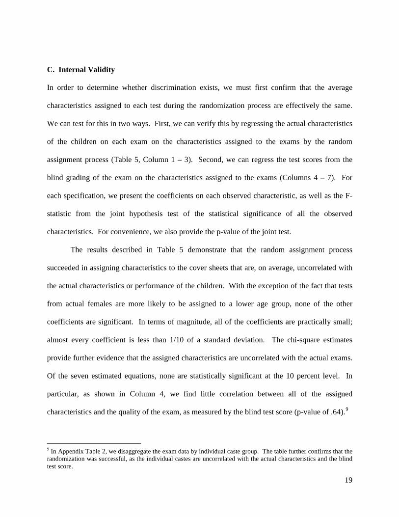
C. Internal Validity

In order to determine whether discrimination exists, we must first confirm that the average

characteristics assigned to each test during the randomization process are effectively the same.

We can test for this in two ways. First, we can verify this by regressing the actual characteristics

of the children on each exam on the characteristics assigned to the exams by the random

assignment process (Table 5, Column 1 – 3). Second, we can regress the test scores from the

blind grading of the exam on the characteristics assigned to the exams (Columns 4 – 7). For

each specification, we present the coefficients on each observed characteristic, as well as the F-

statistic from the joint hypothesis test of the statistical significance of all the observed

characteristics. For convenience, we also provide the p-value of the joint test.

The results described in Table 5 demonstrate that the random assignment process

succeeded in assigning characteristics to the cover sheets that are, on average, uncorrelated with

the actual characteristics or performance of the children. With the exception of the fact that tests

from actual females are more likely to be assigned to a lower age group, none of the other

coefficients are significant. In terms of magnitude, all of the coefficients are practically small;

almost every coefficient is less than 1/10 of a standard deviation. The chi-square estimates

provide further evidence that the assigned characteristics are uncorrelated with the actual exams.

Of the seven estimated equations, none are statistically significant at the 10 percent level. In

particular, as shown in Column 4, we find little correlation between all of the assigned

characteristics and the quality of the exam, as measured by the blind test score (p-value of .64).9

9 In Appendix Table 2, we disaggregate the exam data by individual caste group. The table further confirms that the randomization was successful, as the individual castes are uncorrelated with the actual characteristics and the blind test score.

20

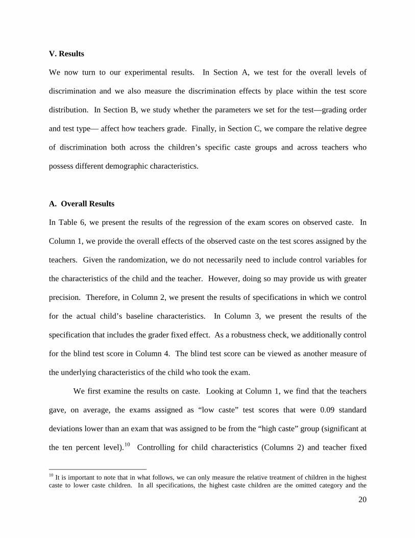
V. Results

We now turn to our experimental results. In Section A, we test for the overall levels of

discrimination and we also measure the discrimination effects by place within the test score

distribution. In Section B, we study whether the parameters we set for the test—grading order

and test type— affect how teachers grade. Finally, in Section C, we compare the relative degree

of discrimination both across the children’s specific caste groups and across teachers who

possess different demographic characteristics.

A. Overall Results

In Table 6, we present the results of the regression of the exam scores on observed caste. In

Column 1, we provide the overall effects of the observed caste on the test scores assigned by the

teachers. Given the randomization, we do not necessarily need to include control variables for

the characteristics of the child and the teacher. However, doing so may provide us with greater

precision. Therefore, in Column 2, we present the results of specifications in which we control

for the actual child’s baseline characteristics. In Column 3, we present the results of the

specification that includes the grader fixed effect. As a robustness check, we additionally control

for the blind test score in Column 4. The blind test score can be viewed as another measure of

the underlying characteristics of the child who took the exam.

We first examine the results on caste. Looking at Column 1, we find that the teachers

gave, on average, the exams assigned as “low caste” test scores that were 0.09 standard

deviations lower than an exam that was assigned to be from the “high caste” group (significant at

the ten percent level).10

10 It is important to note that in what follows, we can only measure the relative treatment of children in the highest caste to lower caste children. In all specifications, the highest caste children are the omitted category and the

Controlling for child characteristics (Columns 2) and teacher fixed

21

effects (Column 3) does not significantly affect the estimate on the lower caste indicator

variable, but the addition of the controls improves the precision of the estimates, which are now

statistically significant at the five percent level. The addition of the blind test score causes the

point estimate to fall to -0.027 (Column 3). The estimate, however, remains statistically

significant at the ten percent level.

Our results suggest that while discrimination may be present, the magnitude of the overall

effect is relatively small when compared to the actual differences in test scores across the caste

groups. The caste gap due to discrimination from our preferred specification in Column 3

(including teacher fixed effects and original characteristics control variables) is -0.086, which is

much smaller than the actual 0.41 standard deviation gap described in Table 3.11

Interestingly, we do not find any effect of assigned gender or age on total test scores,

regardless of specification (Table 6). Note that in addition to not being significant, the

The effect size

falls within the lower tail of the distribution of the impacts of various education interventions in

the developing world that have been evaluated by randomized experiments. Successful

interventions have typically fallen within a 0.07 to 0.24 standard deviation range; this range

includes evaluations of programs that provide additional teachers (Banerjee, Cole, Duflo, and

Linden, 2007), teacher monitoring and incentive programs (Duflo, Hanna, and Ryan, 2007;

Glewwe, Illias, and Kremer, 2003), tracking programs (Duflo, Dupas, and Kremer, 2008),

scholarships for girls (Kremer, Miguel, and Thornton, 2007), and contract teachers

(Muralidharan and Sundararaman, 2008).

indicator variable for the lower castes measures the difference between the lower castes and the highest caste. We cannot assess, for example, whether teachers are biased in favor of high caste children or against lower caste children. 11The finding that discrimination accounts for only a small percentage of the difference between groups has been documented in other settings, such as Levitt (2004), who finds that, when discrimination is present, it is not the leading factor of how people vote in the game show the weakest link.

22

magnitudes of the effects are very small. For example, being labeled with an additional year of

age provides between a 0.001 – 0.003 increase in score.

In Table 7, we test whether the underlying exam quality influences the teacher’s actions.

In Column 1, we interact the blind test score with the observed characteristics and control for the

blind test score, using the following equation:

ijjjijiijiijij wzqvqvy ετδηλβ +++++= * (5)

where iq is the blind test score for test i. We find that the teachers grade the low caste exams

down by 0.029 standard deviations. However, possessing a higher quality exam mitigates this

effect. Specifically, a one standard deviation increase in the blind test score leads to a 0.03

standard deviation increase in the difference between the low caste and high caste groups

(statistically significant at the ten percent level).

We next create a variable that indicates whether an exam possesses a high underlying

quality. Specifically, the variable equals 1 if the blind test score is above average and equals

zero otherwise. We then estimate a specification that includes the interactions of this variable

with each of the assigned demographic characteristics. We find that teachers grade the below

average exams that were assigned to be low caste down by -0.108 standard deviations

(statistically significant at the 5 percent level). However, they grade the exams that are high

quality up by 0.083; however, it is important to note that this effect is only statistically

significant at the 20 percent level. Thus, there is some evidence that teachers help low caste

children who show some promise, but hurt low caste children that match perceived stereotypes.

Interestingly, we also see that teachers grade low quality exams that were assigned to be female

up by 0.107 standard deviations (significant at the 1 percent level), but then grade the high

quality exams down by the almost the same magnitude (significant at the 1 percent level). Thus,

23

while on average girls do not appear to be discriminated against, top performing girls tend to be

assigned lower grades than high performing boys for similar quality work.

To provide additional detail on the relationship between caste discrimination and test

quality, we construct a non-parametric estimate of the relationship between the score assigned to

the exam and the score from the blind grading. The estimates are constructed using a local linear

polynomial estimator (bandwidth of 0.4) and are presented in Figure 2. The solid line represents

the scores assigned to tests labeled as high caste and the dashed line represents the scores

assigned to the tests labeled as lower caste. There is a clear break that emerges in the data at

about -1.1 standard deviations, in which the high caste children are consistently scored higher

than the lower caste children. To estimate this directly, we interact the lower caste indicator with

an indicator for having a blindly graded score below -1.1 standard deviations (Column 3 of Table

7). Consistent with Figure 2, lower caste children with a blind test score below -1.1 standard

deviations score, on average, -0.15 standard deviations lower than their high caste peers.

B. Parameters of the Exam

In addition to discriminating for (or against) particular types of children, it is also possible that

teachers may be more likely to discriminate in particular types of situations. To explore these

types of issues, we incorporated two features into the exam: the random ordering of grading and

exam sections with varying levels of subjectivity.

For each teacher, we created a packet in which we specified the order in which teachers

should grade the exam. Therefore, for each teacher, we know which exams were graded first and

which exams were graded towards the end. Using this knowledge, we can test whether teachers

discriminate more at the start of the packet, when they were first getting used to the format of the

24

particular test. In Column 1 of Table 8, we show the results between the interaction of the

observed characteristics and the place in the grading order (which varies by teacher from 1 to

25), controlling for the place in the grading order in which the exam was graded. In Column 2,

we show the results of the interaction between the observed characteristics and a variable that

indicates that the exam was graded in the first half of the teacher’s pile. All regressions include

the original test characteristics and the grader fixed effect.

We find that the grading order matters. Teachers mark exams that are assigned to be low

caste 0.23 standard deviations lower (significant at the 5 percent level; Column 1). However, as

grading order increases, the difference is mitigated. As shown in Column 2, being graded in the

first half of the packet implies a 0.12 standard deviation gap between the exams that were

assigned to be low and high caste (although this is only significant at about the 20 percent level)

and a 0.10 gap between the exams that were assigned to be female and male (significant at the 1

percent level). Figure 3 illustrates this low versus high caste comparison graphically. The x-axis

is the order in which the exams were graded. The dotted line signifies the assigned scores for the

low caste group, while the straight line signifies this for the high caste group. As in the

regression analysis, we find a gap in test scores between the low and high caste groups at the

start of the grading order, but this effect fades as the place in the grading order increases.

Taken together, these results start to suggest that when teachers are not confident with a

testing instrument, discrimination is most likely to occur. It appears that when grading students

early in the process, when the overall distribution of scores is unknown, teachers may use the

caste of a student not as a signal of performance, but rather as a signal of where the child will

eventually land in the overall distribution of tests. This also suggests that programs that improve

teacher skills and comfort level with testing instruments, may also potentially reduce the

25

discrimination seen in the classroom. While this is not something we can fully verify in the

context of this particular experiment, it provides guidance for future work.

The second feature we attempted to incorporate into the exam was the level of

subjectivity of the exam questions. It is possible, for example, that the effects may be small if

the teachers have little leeway in assigning points to the exam questions. We specifically

included sections on the exam that had different levels of subjectivity. And as demonstrated in

Table 2, the relative subjectivity of these sections is borne out by the significantly lower

correlations between blind and non-blind scores on the exam’s art section relative to the other

sections. In Table 9, we present the results disaggregated by subject. All specifications include

the original test characteristics and grader fixed effects as controls. Interestingly, we do not see

significant differences across the three subjects. Even on the art section, the observed reduction

in test scores for lower caste students is similar to the estimates for the math section.

To better understand these results, we took a closer look at the points assigned for each

question on the exam. We did not give the teachers advice about how to assign points for each

question; we only provided guidance on the maximum number of possible points per question.

Despite the fact that the questions on the test were relatively simple, the graders still made an

effort to assign students partial credit for the questions on the Hindi section (and also, to a lesser

degree, the math section). Therefore, even though the art exam was the most subjective, in the

end, all exams provided the teachers with some level of discretion.

C. Specific Characteristics of the Child and Teacher

We, next, explore whether the results differ by the specific caste group of the child and whether

different types of teachers exhibit different degrees of discrimination.

26

In Table 10, we show the results by disaggregated caste groups. While observed gender

and age are still included in the specification, the results are near identical to Table 6 and,

therefore, we omit them from the tables for conciseness. All specifications also include the

original test characteristics and grader fixed effects. In Column 1, we show the main effects of

each caste. In Columns 2 and 3, we provide the results of specifications that include the

interaction of the caste variable with the blind test score and an indicator variable for an above

average score on the blind test, respectively. Recall that the caste groups in terms of descending

order of prestige are the Kshatriya, Vaishya, and Shudra.

We find significant differences between the exams that were assigned as belonging to the

high caste groups and exams that were assigned as belonging to either the Kshatiya and Shudra

groups (Column 1); the effect on exams that were assigned as belonging to the Vaishya group,

while negative, is not significant at conventional levels (significant at 15% level). We cannot

reject the hypothesis that the coefficients on the three observed caste variables are significantly

different from one another. The results from Column 2 and Column 3 are consistent with those

from Table 7. Having an above average test scores increases the average scores for individuals

labeled as the lower caste groups, relative to those labeled as high caste. This effect is

particularly strong for the highest of the low caste groups (Kshatriya).

Finally, we explore whether teachers differ in the degree to which they use students’

observed characteristics as proxies for actual performance. We focus on the four key

characteristics that are the most theoretically relevant. First, we explore whether the caste and

gender of the teacher affects the observed levels of discrimination. For example, teachers’

beliefs on the average characteristics of children from a particular caste may be influenced by

their own caste. Lower caste teachers, for example, may be less likely to use caste as a proxy for

27

performance given their intimate experience with low caste status or may feel partial towards

helping someone from their own social group (in-group bias). On the other hand, such teachers

may have internalized a belief in the difference in ability as a means of rationalizing historical

experience. Thus, low caste teachers may discriminate more against very low status children.12

We do not find evidence of in-group bias. In fact, we observe the opposite. We do not

see any difference in test scores between exams assigned as belonging to the lower caste and

We test for the presence of in-group bias among the teachers in our sample in regards to caste

and gender. In addition, we estimate whether the degree of discrimination varies by the teachers’

education levels or age. More educated teachers may be more aware of and more tolerable of

diversity, whereas older teachers may have more experience with individuals of different

backgrounds or more experience with children of various backgrounds through more teaching

experience.

We present the results of our analysis in Table 11. We present the results by caste,

gender, master’s degree completion, and age in Panels A through D, respectively. In Column 1,

we show the results for the sample that is listed in the panel title, while in Column 2, we show

the results for the remaining teachers. In Column 3, we present the difference between the

coefficients. In Column 4, we present results of a specification that includes the interactions

between the observed caste variables and all four teacher demographic variables. All regressions

include both original test characteristics and grader fixed effects.

12 Previous studies exploring how belonging to a group impacts a person’s treatment of others in that group have found, for the most part, evidence of in-group bias (positive discrimination towards members of your own group). A series of experiments in the psychology literature have found that individuals presented in-group bias in even in artificially constructed groups (Vaughn, Tajfel, and Williams, 1981) or groups that were randomly assigned (Billig and Tajfel, 1973). Turner and Brown (1978) studied “in-group bias” when “status” is conferred to the groups, and found that while all subjects were biased in favor of their own group, the groups identified as superior exhibited more in-group bias. More recently, Klein and Azzi (2001) also find that both “inferior” and “superior” groups gave higher scores to people in their own group. Using data from the game show “The Weakest Link,” Levitt (2004) find that some evidence that men vote more for men and women vote more for women. For a good description of theory and literature of in-group bias the work of Anderson, Fryer, and Holt (2006).

28

those assigned as belonging to the high caste for teachers of the high caste (Column 1, Panel A).

However, low caste teachers (Column 2) seem to have discriminated significantly against

members of their own group. The difference between low and high caste teachers is large –about

0.2 standard deviations—and significant at the 10 percent level (Column 3). Of course, as

described in Table 1, lower caste teachers tend to come from a different socio-economic

background than upper caste teachers (more likely to be male, less likely to have a master’s

degree, etc), and these characteristics may account for the results we find, rather than caste. To

control for these possible confounds, in Column 4, we control for both the main characteristics

and the interactions of the characteristics with the observed low caste status. The results remain

the same: lower caste teachers significantly downgrade exams that are assigned to be lower

caste, relative to the high caste teachers.

Turning to gender, we also do not observe in-group bias. We do not see a significant

difference in the way female and male teachers grade exams that are randomly assigned to be

male versus female. In terms of caste, we observe that female teachers significantly grade down

low caste exams, while male teachers do not. However, the coefficient of the effects for male

teachers is not significantly different than the coefficient for female teachers. Moreover, while

the coefficients are similar, the sample size of the male teachers is much smaller (33 male

teachers versus 87 female teachers), which may account for the higher variance in the estimates

for the male teachers.

While we find no significant difference in caste discrimination by teachers’ education or

age, we find that more educated teachers and older teachers are more likely to give higher grades

to exams that were assigned to be female.

29

VI. DISCUSSION

We find that teachers provide exams that are assigned to be “lower caste” scores that are about

0.03 to 0.09 standard deviations lower than those that are assigned to be “high caste.” What is

the underlying model that drives these results? Economic theories of discrimination fall into two

main categories. The first type of models falls under the category of taste-based discrimination,

in which teachers may have particular preferences for individuals of a particular group or

characteristic. The second class of theories encompasses statistical discrimination, in which

teachers may use observable characteristics to proxy for unobservable skills.

The empirical design should eliminate the possibility of statistical discrimination, as

teachers observe a measure of skill for the child: the actual performance on the exam. However,

one can imagine a series of situations where the teacher may statistically discriminate. First, the

teacher may be lazy, and may not be invested in carefully studying the exam to determine the

skill level for each child. Thus, they may use the demographic variables to instead proxy for

skill. While we cannot fully rule out this story, the fact that the teachers knew that a fairly large

prize was at stake increased the seriousness of the exercise When they were confused, the

teachers asked the project team questions on the grading and all of the teachers seemed to spend

a fair bit of time grading each exam. Moreover, if teachers were lazy, we may expect them to

mark wrong answers as “0” right away, and not spend time thinking through the answer to

determine the correct level of partial credit. In fact, we observe the opposite: teachers gave a

considerable amount of partial credit for wrong answers. Thus, it does not appear as though the

teachers were slacking.

Second, teachers may statistically discriminate if they are not confident about the testing

instrument. In particular, teacher may be unsure about what is the right level of partial credit to

30

give per question and they may be also unsure about what the final distribution of grades will

look like. Thus, teachers may use the characteristics of a child, not as a signal of performance,

but rather as a signal of where the child will end up in the distribution. The data lends some

credence to this theory: discrimination tends to occur at the start of the grading order and fades

over time.

On the other hand, there is also considerable evidence that the discrimination is taste-

based. First, if we expected the teachers to be statistically discriminating, we would expect them

to use observed age to make predictions on the skills of the child, as the age variable has much

more predictive power on test scores than caste. However, they tend to discriminate on caste,

but not age. Thus, these results can imply taste-based discrimination, rather than just statistical

discrimination. Note, however, that we cannot rule out the fact that teachers have incomplete

information, or are just bad at making statistical predictions of how children of particular groups

will fare on the exams.

Second, the gap in scores based on demographics varies by the quality of the exam: low

caste children are hurt when their exam quality is low to begin with and females are hurt when

their exams are of high quality. If the teachers were conducting statistical discrimination, we

may not expect quality to matter as much.

VII. CONCLUSION

While education has the power to transform the lives of the poor, children who belong to

traditionally disadvantaged groups may not reap the full benefits of education if teachers

systematically discriminate against them. Through an experimental design, we find evidence

that teachers discriminate against low caste children in grading exams. For example, we find

31

teachers give exams that are assigned to be upper caste test scores that are, on average, 0.03 to

0.09 standard deviations higher than those assigned a lower caste classification. We do not find

any overall evidence of discrimination by gender or age. Disaggregating the results by the

quality of the exam, the low-performing low caste children and top-performing females tend to

lose out the most due to discrimination. Quite interestingly, we find that the discrimination

against low caste students is driven by low caste teachers, while those teachers from the higher

caste do not appear to discriminate at all.

It is important to note that our study only reflects upon one element of discrimination

within the classroom. Discrimination may also exist in other forms: calling on students of

particular groups but not others, discouraging those of certain groups from furthering their

education, and so forth. If, as we show, discrimination exists in the subtle grading of an exam,

other more blatant types of discrimination may exist as well. Therefore, our results provide

additional motivation for research to investigate how the treatment of children within the

classroom differs by race, ethnicity, and gender.

VIII. WORKS CITED Anderson, Lisa, Roland Fryer and Charles Holt (2006) “Discrimination: Experimental Evidence from Psychology and Economics,” in William M. Rogers, ed. Handbook on the Economics of Discrimination. Northampton, MA: Edward Elgar. Arrow, Kenneth (1972) “Models of Job Discrimination,” in A. H. Pascal, ed. Racial Discrimination in Economic Life. Lexington, MA: D. C. Health, 83-102. Banerjee, Abhijit and Marianne Bertrand, Saugato Datta, and Sendhil Mullainathan (2009) “Labor Market Discrimination in Delhi: Evidence from a Field Experiment,” Journal of Comparative Economics. 37(1): 14-27. Banerjee, Abhijit, Shawn Cole, Esther Duflo, and Leigh Linden (2007) "Remedying Education: Evidence from Two Randomized Experiments in India," Quarterly Journal of Economics 122(3): 1235-1264.

32

Banerjee, Biswajit and J.B. Knight (1985) “Caste Discrimination in the Indian Urban Labour Market,” Journal of Development Economics. 17(3): 277-307. Bertrand, Marianne, Rema Hanna, and Sendhil Mullainathan (2008) “Affirmative Action in Education: Evidence from Engineering College Admissions in India,” NBER Working Papers. No 13926. Bertrand, Marianne and Sendhil Mullainathan (2004) “Are Emily and Greg More Employable than Lakisha and Jamal? A Field Experiment on Labor Market Discrimination,” American Economic Review. 94(4): 991-1013. Billig, Michael and Tajfel, Henri (2009) “Social Categorization and Similarity in Intergroup Behavior,” European Journal of Social Psychology. 3(1): 27-52. Chandra, V.P. (1997) “Remigration: Return of the Prodigals: An Analysis of the Impact of the Cycles of Migration and Remigration on Caste Mobility,” International Migration Review. 31(1): 1220-1240. Coate, Steven and Glenn Loury (1993) “Will Affirmative Action Eliminate Negative Stereotypes?” American Economic Review. 83(5): 1220-1240. Deshpande, Ashwini and Katherine Newman (2007) “Where the Path Leads: The Role of Caste in Post-University Employment Expectations,” Economic and Political Weekly. 42(41): 4133-4140. Duflo, Esther, Pascaline Dupas and Michael Kremer (2008) “Peer Effects and the Impact of Tracking: Evidence from a Randomized Evaluation in Kenya,” CEPR Discussion Paper Series, No DP7043. Duflo, Esther, Rema Hanna, and Stephen Ryan (2008) “Monitoring Works: Getting Teachers to Come to School,” CEPR Discussion Paper Series, No. DP6682. Ferguson, Ronald (2003) “Teachers’ Perceptions and Expectations and the Black-White Test Score Gap,” Urban Education. 38(4): 460-507. Fix, M. and R. Struyk (1994) Clear and Convincing Evidence. Washington, DC: The Urban Institute. Glewwe, Paul, Nauman Ilias, and Michael Kremer (2003) “Teacher Incentives,” NBER Working Paper Series, No. 9671. He, Fang, Leigh Linden, and Margaret MacLeod (2008) “How to Teach English in India: Testing the Relative Productivity of Instruction Methods within the Pratham English Language Education Program,” Working Paper. Columbia University Department of Economics.

33

Hoff, Karla and Priyanka Pandey (2006) “Discrimination, Social Identity, and Durable Inequalities,” American Economic Review, Papers and Proceedings. 96(2): 206-211. Holla, Alaka (2007) “Caste Discrimination in School Admissions: Evidence from Test Scores,” Working paper, Innovations for Poverty Action. Jodhka, Surinder S. and Katherine Newman (2007) “In the Name of Globalisation: Meritocracy, Productivity and the Hidden Language of Caste,” Economic and Political Weekly. 42(41): 4125- 4132. Klein, Oliver and Assad Azzi (2001) “Do High Status Groups Discriminate More? Differentiation Between Social Identity and Equity Concerns,” Social Behavior & Personality. 29(3): 209-221. Kremer, Michael, Edward Miguel, and Rebecca Thornton (2009) “Incentives to Learn,” Forthcoming. Review of Economics and Statistics. Lakshmanasamy, T. and S. Madeshwaran (1995) “Discrimination by Community: Evidence from Indian Scientific and Technical Labour Market,” Indian Journal of Social Science. 8(1): 59-77. Lavy, Victor (2008) “Do Gender Stereotypes Reduce Girls’ or Boys’ Human Capital Outcomes? Evidence from a Natural Experiment,” Journal of Public Economics. 92(10-11): 2083-2105. Levitt, Steven (2004) “Testing Theories Of Discrimination: Evidence From Weakest Link,” Journal of Law and Economics. 47(2): 431-452. Madheshwaran, S. and Paul Attewell (2007) “Caste Discrimination in the Indian Urban Labour Market: Evidence from the National Sample Survey,” Economic and Political Weekly. 42(41): 4146-4153. Mechtenberg, Lydia (2008) “Cheap Talk in the Classroom: How Biased Grading at School Explains Gender Differences in Achievements, Career Choices, and Wages,” Forthcoming Review of Economic Studies. Munshi, Kaivan and Mark Rosenzweig (2006) “Traditional Institutions Meet the Modern World: Caste, Gender, and Schooling Choice in a Globalizing Economy,” American Economic Review. 96(4): 1225-1252. Muralidharan, Karthik and Venkatesh Sundararaman (2008) "Contract Teachers: Experimental Evidence from India" Working Paper, University of California at San Diego Department of Economics. The PROBE Report (1999) Public Report on Basic Education in India. New Delhi, India: Oxford University Press.

34

Rao, V. (1992) “Does Prestige Matter? Compensating Differential for Social Mobility in the Indian Caste System,” University of Chicago Economics Research Center Working Paper Series, No. 92-6. Shastry, Gauri Kartini and Leigh Linden (2008) “Identifying Agent Discretion: Exaggerating Student Attendance in Response to a Conditional School Nutrition Program,” Working paper, Columbia University Department of Economics. Siddique, Zahra (2008) “Caste Based Discrimination: Evidence and Policy,” IZA Discussion Paper Series. No 3737. Steele, Claude and Joshua Aronson (1998) “Stereotype Threat and the Intellectual Test Performance of African-Americans,” Journal of Personality and Social Psychology. 69(5): 797-811. Taijel, Henri (1970) “Experiments in Inter-Group Discrimination,” Scientific American. 223(5): 96-102. Unni, Jeemol (2002) “Earnings and Education among Ethnic Groups in India,” Gujarat Institute of Development Research Working Paper Series, No. 124. Vaughan, G. M., Tajfel, H., and Williams, J. (1981). “Bias in reward allocation in an intergroup and an interpersonal context,” Social Psychology Quarterly, 44(1), 37-42.

AllHigh Caste Low Caste Female Male No Master's Master's

Characteristic (1) (2) (3) (4) (5) (6) (7)Number of teachers 120 81 39 87 33 61 59

Upper Caste 0.68 1.00 0.00 0.75 0.48 0.61 0.75

Female 0.73 0.80 0.56 1.00 0.00 0.67 0.78

Age 35.33 36.77 32.33 36.33 32.67 32.92 37.81

Less than a Master's Degree 0.51 0.46 0.62 0.47 0.61 1.00 0.00

Private School 0.56 0.49 0.69 0.49 0.73 0.70 0.41

Closest Friend: Same Caste Grouping 0.64 0.74 0.44 0.72 0.42 0.66 0.63

Belong to a Caste Association 0.41 0.39 0.46 0.44 0.33 0.42 0.41

0.81 0.83 0.77 0.82 0.79 0.80 0.81

1. This table summarizes the characteristics and beliefs of the 120 teachers who participated in the grading sessions.

Table 1: Characteristics of the Teachers

A. Teacher Characteristics

B. Teacher Beliefs

Notes:

Believe that teachers favor some students over others in their grading for reasons unrelated to their educational performance

Caste Gender Education

Original Observed(1) (2)

Brahmin 0.18 0.12(0.39) (0.33)

Kshatriya 0.24 0.12(0.43) (0.33)

Vaishya 0.34 0.50(0.47) (0.50)

Shudra 0.06 0.25(0.23) (0.43)

Unknown Caste/Not Hindu 0.18(0.38)

Female 0.44 0.50(0.50) (0.50)

Age 10.95 10.98(2.04) (2.00)

Notes:

2. The original (true) characteristics, listed in Column 1, includedata on all 69 children who completed a test and a demographicsurvey. 3. Column 2 provides data on the characteristics that wererandomly assigned to the cover sheets of the tests that the teachersgraded. This column summarizes the data from the 3,000coversheets in the study (25 for each of 120 teachers).

Table 2: Child Characteristics

A. High Caste

C. Other

B. Lower Caste

1. This table summarizes both the real characteristics of thechildren in our sample and the characteristics observed by theteachers.

Teacher Scores Blind Test Score(1) (2)

Table 3: Description of Test Scores

(1) (2)

Total 0.63 0.67(0.19) (0.19)

Math 0.68 0.70

A. Test Score

B. Test Scores, By Exam

(0.22) (0.23)Hindi 0.55 0.58

(0.16) (0.16)Art 0.47 0.64

(0.32) (0.35)

Observations 3000 69Observations 3000 69Notes:1. This table summarizes the test scores from the exam tournament. The scores arepresented in terms of the percentage of total possible points.2. Column 1 provides data on the 3,000 exams that were graded by the 120 teachers inthe study. Column 2 provides the results from a blind grading of the original 69exams.

Figure 1: Range Per Given Test

0 9

1

0.2

0.3

0.4

0.5

0.6

0.7

0.8

0.9

1

Notes:1. Figure 1 provides the range of test scores (in percentages) given by the teachers for

0

0.1

0.2

0.3

0.4

0.5

0.6

0.7

0.8

0.9

1

1 11 21 31 41 51 61

1. Figure 1 provides the range of test scores (in percentages) given by the teachers foreach of the 69 exams used in the study.

0

0.1

0.2

0.3

0.4

0.5

0.6

0.7

0.8

0.9

1

1 11 21 31 41 51 61

Test Type: Total Total Math Hindi Art(1) (2) (3) (4) (5)

Constant -5.348 -0.927 -0.941 -0.97 -1.094(0.416)*** (0.164)*** (0.169)*** (0.191)*** (0.330)***

Low Caste -0.409 -0.013 -0.026 0.008 -0.111(0.037)*** (0.014) (0.015)* (0.017) (0.029)***

Female 0.183 -0.011 0.006 -0.001 0.004(0.029)*** (0.011) (0.012) (0.013) (0.023)

Age 0.846 0.142 0.164 0.133 0.147(0.079)*** (0.031)*** (0.032)*** (0.036)*** (0.062)**

Age^2 -0.03 -0.006 -0.007 -0.005 -0.007(0.004)*** (0.001)*** (0.001)*** (0.002)*** (0.003)**

Blind Test Score 0.926 0.929 0.932 0.634(0.007)*** (0.007)*** (0.008)*** (0.014)***

Observations 3000 3000 3000 3000 3000R-squared 0.28 0.89 0.9 0.85 0.5

4. Results that are statistically significant at the one, five, and ten percent levels are indicated by ***, **, and *respectively.

Table 4: Correlations between Original Characteristics and Final Test Scores

Note: 1. This table contains the raw correlations between the grades awarded to the exams by teachers and thechildren's original, unobserved characteristics. 2. The first two columns contain results for the total test score, with and without controlling for the blind testscores. Columns 3 - 5 present the results, controlling for the blind test score, by exam section.3. Child performance on each exam is measured using the score normalized to the overall exam scoredistribution.

Low Caste Female Age Total Math Hindi Art(1) (2) (3) (4) (5) (6) (7)

Low Caste -0.035 0.006 -0.071 -0.068 -0.062 -0.064 -0.054(0.021) (0.027) (0.113) (0.054) (0.055) (0.054) (0.055)

Female -0.02 -0.022 -0.022 0.012 0.031 -0.001 -0.02(0.014) (0.018) (0.075) (0.036) (0.036) (0.036) (0.036)

Age -0.063 -0.100 0.053 -0.014 0.045 -0.076 -0.007(0.045) (0.058)* (0.237) (0.114) (0.115) (0.114) (0.115)

Age^2 0.003 0.004 -0.003 0.001 -0.002 0.003 0.000(0.002) (0.003)* (0.011) (0.005) (0.005) (0.005) (0.005)

Observations 3000 3000 3000 3000 3000 3000 3000

F-Stat 1.85 1.17 0.25 0.43 0.64 0.48 0.89P-Value 0.1157 0.3215 0.9082 0.7889 0.6358 0.7501 0.4682Note:

3. Results that are statistically significant at the one, five, and ten percent levels are indicated by ***, **, and * respectively.

Table 5: Randomization CheckBlind ScoresActual Characteristics

1. This table contains regressions of the actual characteristics of the children of each exam on the characteristics randomlyassigned to the coversheet on the copy of the exam that was graded by a teacher.2. The F-statistic and p-value provide a test of joint significance of the observed characteristics.

Observed Characteristics (1) (2) (3) (4)Low Caste -0.09 -0.087 -0.086 -0.027

(0.054)* (0.044)** (0.043)** (0.017)*Female 0.022 0.015 0.014 0.008

(0.036) (0.029) (0.029) (0.011)Age 0.001 0.003 0.003 0.001

(0.009) (0.007) (0.007) (0.003)

Original Test Characteristics YES YES YESGrader Fixed Effect YES YESBlind Test Score YESNote:

3. Results that are statistically significant at the one, five, and ten percent levels are indicated by ***, **, and * respectively.

Table 6: Effect of Observed Characteristics on Total Test Scores

1. Table 5 presents the regression of total normalized test scores on observed characteristics that were randomly assigned to the coversheets of test copies. 2. The sample includes the 3,000 graded exams (graded in sets of 25 by 120 teachers).

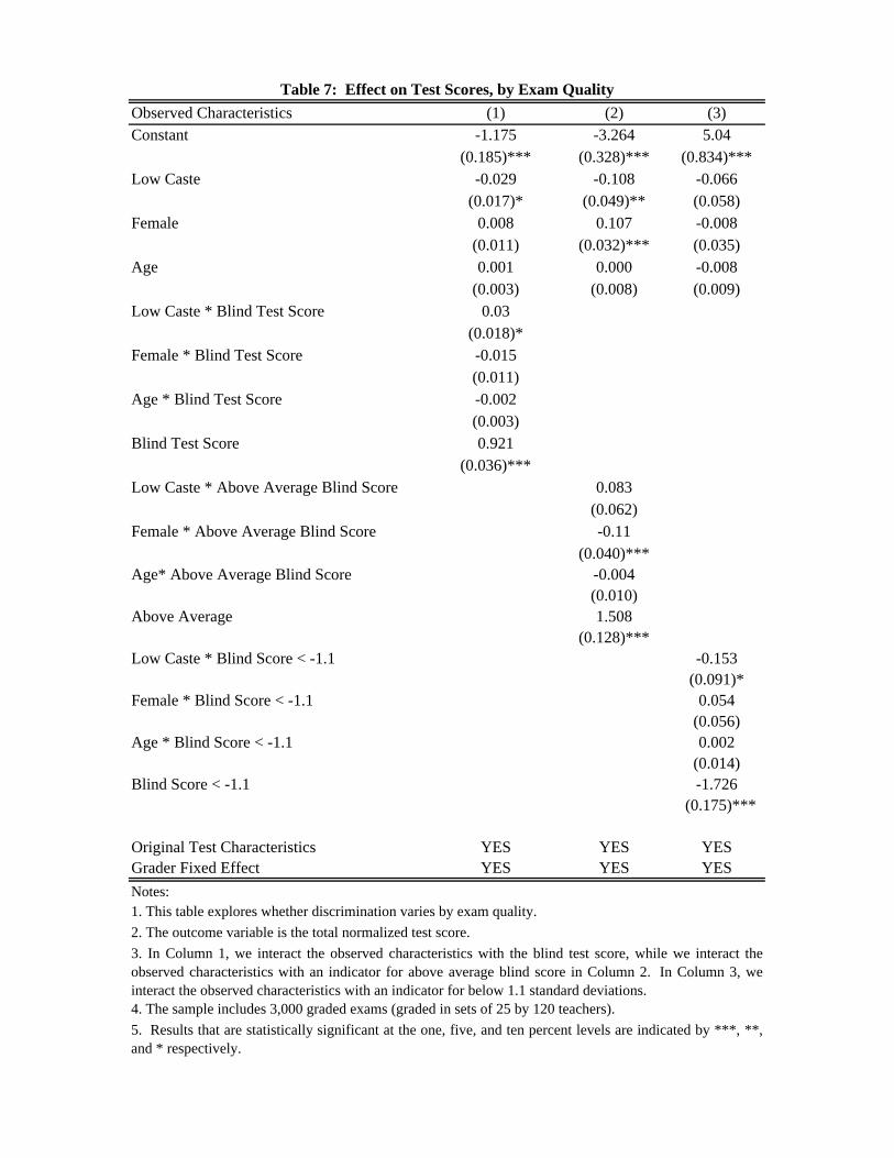
Observed Characteristics (1) (2) (3)Constant -1.175 -3.264 5.04

(0.185)*** (0.328)*** (0.834)***Low Caste -0.029 -0.108 -0.066

(0.017)* (0.049)** (0.058)Female 0.008 0.107 -0.008

(0.011) (0.032)*** (0.035)Age 0.001 0.000 -0.008

(0.003) (0.008) (0.009)Low Caste * Blind Test Score 0.03

(0.018)*Female * Blind Test Score -0.015

(0.011)Age * Blind Test Score -0.002

(0.003)Blind Test Score 0.921

(0.036)***Low Caste * Above Average Blind Score 0.083

(0.062)Female * Above Average Blind Score -0.11

(0.040)***Age* Above Average Blind Score -0.004

(0.010)Above Average 1.508

(0.128)***Low Caste * Blind Score < -1.1 -0.153

(0.091)*Female * Blind Score < -1.1 0.054

(0.056)Age * Blind Score < -1.1 0.002

(0.014)Blind Score < -1.1 -1.726

(0.175)***

Original Test Characteristics YES YES YESGrader Fixed Effect YES YES YESNotes:

5. Results that are statistically significant at the one, five, and ten percent levels are indicated by ***, **,and * respectively.

4. The sample includes 3,000 graded exams (graded in sets of 25 by 120 teachers).

Table 7: Effect on Test Scores, by Exam Quality

1. This table explores whether discrimination varies by exam quality.2. The outcome variable is the total normalized test score.3. In Column 1, we interact the observed characteristics with the blind test score, while we interact theobserved characteristics with an indicator for above average blind score in Column 2. In Column 3, weinteract the observed characteristics with an indicator for below 1.1 standard deviations.

Figure 2: The Caste Gap, by Blind Test Score

Observed Characteristics (1) (2)Constant -5.657 -5.872

(0.500)*** (0.479)***Low Caste -0.233 -0.03

(0.093)** (0.058)Female -0.098 0.063

(0.060) (0.040)Age 0.004 -0.002

(0.015) (0.010)Low Caste * Grading Order 0.011

(0.006)*Female * Grading Order 0.009

(0.004)**Age * Grading Order 0.000

(0.001) Grading Order -0.014

(0.013)Low Caste * Start of Grading Order -0.120

(0.089)Female * Start of Grading Order -0.102

(0.058)*Age* Start of Grading Order 0.01

(0.015)Start of Grading Order 0.035

(0.184)

Original Test Characteristics YES YESGrader Fixed Effect YES YESNote:

5. Results that are statistically significant at the one, five, and ten percent levels are indicatedby ***, **, and * respectively.

4. The sample includes 3,000 graded exams (graded in sets of 25 by 120 teachers).

Table 8: Effect on Test Scores, by Grading Order

2. Grading order is a variable that gives the order of the exam as graded by the teacher. Thisvariable ranges from 1 (1st exam graded) to 25 (last exam graded). Start of grading order is anindicator variable that equals one if grading order is less than or equal to twelve, and zerootherwise.

1. This table explores whether the order in which the exam was graded affects the treatment ofexams assigned by observable characteristics.

3. The outcome variable is the total normalized total score.

Figure 3: The Caste Gap, by Grading Order

Math Hindi Art(1) (2) (3)

Low Caste -0.072 -0.08 -0.058(0.043)* (0.047)* (0.042)

Female 0.024 -0.004 0.011(0.029) (0.031) (0.028)

Age 0.007 0.001 -0.005(0.007) (0.008) (0.007)

Original Test Characteristics YES YES YESGrader Fixed Effect YES YES YESNote:

Table 9: Effect on Test Scores, by Subject

1.This table presents the regression of normalized test scores for the indicated sections ofthe exam on the observed characteristics that were randomly assigned to the coversheets.2. The sample includes 3,000 graded exams (graded in sets of 25 by 120 teachers). 3. Results that are statistically significant at the one, five, and ten percent levels are indicated by ***, **, and * respectively.

Observed Characteristics (1) (2) (3)Constant -5.892 -1.18 -3.275

(0.471)*** (0.185)*** (0.328)***Kshatriya -0.112 -0.03 -0.206

(0.057)* (0.022) (0.065)***Vaishya -0.067 -0.023 -0.083

(0.045) (0.017) (0.051)Shudra -0.112 -0.042 -0.114

(0.050)** (0.019)** (0.056)**Kshatriya * Blind Test Score 0.028

(0.023)Vaishya * Blind Test Score 0.029

(0.018)Shudra * Blind Test Score 0.033

(0.020)Blind Test Score 0.92

(0.037)***Kshatriya * Above Average Blind 0.187

(0.082)**Vaishya * Above Average Blind 0.06

(0.065)Shudra* Above Average Blind 0.081

(0.071)Above Average 1.495

(0.128)***

Original Test Characteristics YES YES YESGrader Fixed Effect YES YES YESNote:

Table 10: Effect of Detailed Caste Groups on Total Test Scores

1. This table presents estimates of the effect of observed caste disaggregated by specific

4. Results that are statistically significant at the one, five, and ten percent levels areindicated by ***, **, and * respectively.

2. The sample includes 3,000 graded exams (graded in sets of 25 by 120 teachers). 3. The outcome variable in all regressions is the normalized total score.

Yes No(1) (2) (3) (4)

Low Caste -0.023 -0.227 0.197 0.204(0.052) (0.078)*** (0.093)** (0.098)**

Female -0.01 0.059 -0.071 -0.058(0.035) (0.051) (0.061) (0.065)

Age 0 0.008 -0.008 -0.01(0.009) (0.013) (0.015) (0.016)

Low Caste -0.064 -0.094 0.031 0.105(0.084) (0.051)* (0.097) (0.103)

Female 0.049 -0.001 0.056 0.03(0.055) (0.034) (0.064) (0.068)

Age 0.009 0.001 0.008 0.007(0.014) (0.008) (0.016) (0.017)

Low Caste -0.079 -0.09 0.011 -0.028(0.062) (0.061) (0.087) (0.089)

Female 0.061 -0.033 0.093 0.127(0.041) (0.040) (0.057) (0.059)**

Age 0.003 0.004 0 0.001(0.010) (0.010) (0.014) (0.015)

Low Caste -0.135 -0.038 -0.099 -0.084(0.061)** (0.062) (0.087) (0.092)

Female 0.061 -0.038 0.098 0.103(0.040) (0.041) (0.057)* (0.061)*

Age 0 0.007 -0.007 -0.009(0.010) (0.010) (0.014) (0.015)

Original Test Characteristics YES YES YES YESGrader Fixed Effect YES YES YES YESNote:

5. Results that are statistically significant at the one, five, and ten percent levels are indicated by ***, **, and * respectively.

1. This table presents estimates of discrimination disaggregated by the characteristics of the teachers.2. Each panel contains four sets of estimates. Estimates presented in column one are for tests graded only by teachers who have thecharacteristics indicated in the panel name. Column two contains estimates using only tests for teachers that do not have the indicatedcharacteristic. Finally, column three presents an estimate of the coefficient on the interaction of the teacher's characteristic with the indicatedobserved child characteristics. Column four presents the same interaction but from a specification that includes interactions with the teachercharacteristics from all of the panels. 3. The sample includes 3,000 graded exams (graded in sets of 25 by 120 teachers). 4. The outcome in every regression is the normalized total score.

A. Upper Caste

B. Male

C. Masters Degree

D. Below Median Age

Table 11: Effect on Test Scores, by Teacher Type

Difference

Difference (Conditional on other teacher characteristics)

Teachers of the indicated category?

Total Total Math Hindi Art(6) (7) (8) (9) (10)

Constant -4.928 -0.929 -0.874 -1.021 -1.054(0.403)*** (0.165)*** (0.171)*** (0.193)*** (0.333)***

Kshatriya -0.161 -0.012 0 -0.01 -0.083(0.042)*** (0.017) (0.018) (0.020) (0.034)**

Vaishya -0.516 -0.016 -0.033 0.003 -0.127(0.039)*** (0.016) (0.017)** (0.019) (0.033)***

Shudra -1.171 -0.012 -0.03 0.042 -0.176(0.068)*** (0.029) (0.030) (0.033) (0.055)***

Unknown -0.336 -0.009 -0.049 0.036 -0.106(0.045)*** (0.018) (0.019)** (0.021)* (0.037)***

Female 0.213 -0.012 0.003 -0.002 0.007(0.028)*** (0.012) (0.012) (0.014) (0.024)

Age 0.781 0.142 0.151 0.143 0.139(0.076)*** (0.031)*** (0.032)*** (0.037)*** (0.063)**

Age^2 -0.027 -0.006 -0.007 -0.006 -0.006(0.004)*** (0.001)*** (0.001)*** (0.002)*** (0.003)**

Blind Test Score 0.926 0.926 0.935 0.631(0.007)*** (0.007)*** (0.009)*** (0.014)***

Observations 3000 3000 3000 3000 3000R-squared 0.34 0.89 0.9 0.85 0.5

Appendix Table 1: Correlations between Original Characteristics and Final Test Scores

Note: 1. This table contains the raw correlations between the grades awarded to the exams by teachers and the children's original,unobserved characteristics. 2. The first two columns contain results for the total test score, with and without controlling for the blind test scores.Columns 3 - 5 present the results, controlling for the blind test score, by exam section.3. Results that are statistically significant at the one, five, and ten percent levels are indicated by ***, **, and *

Brahmin Kshatriya Vaishya Shudra Unknown Female Age Total Math Hindi Art(1) (2) (3) (4) (5) (6) (7) (8) (9) (10) (11)

Kshatriya 0.041 -0.004 -0.039 0.024 -0.023 0.038 -0.199 -0.106 -0.093 -0.111 -0.062(0.028) (0.032) (0.035) (0.017) (0.028) (0.036) (0.150) (0.072) (0.072) (0.072) (0.072)

Vaishya 0.039 -0.026 -0.041 0.016 0.012 0.001 -0.079 -0.059 -0.056 -0.057 -0.035(0.022)* (0.025) (0.027) (0.013) (0.022) (0.029) (0.118) (0.057) (0.057) (0.057) (0.057)

Shudra 0.024 -0.027 0.009 0.007 -0.013 -0.001 0.01 -0.068 -0.061 -0.056 -0.087(0.025) (0.027) (0.030) (0.015) (0.024) (0.031) (0.129) (0.063) (0.063) (0.062) (0.063)

Female 0.02 -0.01 0.006 -0.009 -0.007 -0.021 -0.026 0.011 0.03 -0.002 -0.02(0.014) (0.016) (0.017) (0.008) (0.014) (0.018) (0.075) (0.036) (0.036) (0.036) (0.036)

Age 0.063 -0.034 0.053 -0.032 -0.05 -0.101 0.055 -0.013 0.046 -0.074 -0.005(0.045) (0.050) (0.055) (0.027) (0.045) (0.058)* (0.237) (0.115) (0.115) (0.114) (0.115)

Age^2 -0.003 0.002 -0.002 0.001 0.002 0.004 -0.003 0.001 -0.002 0.003 0(0.002) (0.002) (0.002) (0.001) (0.002) (0.003)* (0.011) (0.005) (0.005) (0.005) (0.005)

Observations 3000 3000 3000 3000 3000 3000 3000 3000 3000 3000 3000

F-Stat 1.38 0.47 1.41 1.06 0.95 1.08 0.61 0.4 0.5 0.48 0.83P-Value 0.2184 0.8309 0.2084 0.3839 0.4613 0.3723 0.7212 0.8798 0.8106 0.8239 0.5469Note:

3. Results that are statistically significant at the one, five, and ten percent levels are indicated by ***, **, and * respectively.2. The F-statistic and p-value provide a test of joint significance of the observed characteristics.

1. This table contains regressions of the actual characteristics of the children on the characteristics randomly assigned to the coversheet of the exam that was graded bythe teachers.

Blind ScoresAppendix Table 2: Randomization Check with Full Set of Caste Variables

Actual Characteristics