Measuring Institutional Investors’ Skill from Their

Investments in Private Equity

Daniel R. Cavagnaro

California State University, Fullerton

Berk A. Sensoy

Ohio State University

Yingdi Wang

California State University, Fullerton

Michael S. Weisbach

Ohio State University and NBER

November 3, 2016

Abstract

Using a large sample of institutional investors’ private equity investments in venture and buyout funds, we

estimate the extent to which investors’ skill affects their returns. We first consider whether investors have

differential skill by comparing the distribution of investors’ returns to a bootstrapped distribution that would

occur if funds were randomly distributed across investors. We find that the variance of actual performance

is higher than that of the bootstrapped distribution, suggesting that higher and lower skilled investors

consistently outperform and underperform. We then extend the Bayesian approach of Korteweg and

Sorensen (2015) to estimate the incremental effect of skill on performance. The results imply that a one

standard deviation increase in skill leads to about a three percentage point increase in returns, suggesting

that variation in institutional investors’ skill is an important driver of their returns.

JEL Classification: G11, G23, G24

Key Words: Institutional Investors, Private Equity, Investment Skill, Markov Chain Monte Carlo

Contact information: Daniel R. Cavagnaro, Department of Information Systems and Decision Sciences, California

State University Fullerton, Fullerton, CA 92834 email: dcavagnaro@fullerton.edu; Berk A. Sensoy, Department of

Finance, Fisher College of Business, Ohio State University, Columbus, OH 43210, email: sensoy.4@osu.edu; Yingdi

Wang, Department of Finance, California State University Fullerton, Fullerton, CA 92834, email:

yingdiwang@fullerton.edu; Michael S. Weisbach, Department of Finance, Fisher College of Business, Ohio State

University, Columbus, OH 43210, email: weisbach.2@osu.edu. Andrea Rossi provided exceptionally good research

assistance. We thank Arthur Korteweg, Ludovic Phalippou, and seminar participants at Berkeley, Fullerton, Georgia

State, Kansas, the 9th Annual London Business School Private Equity Conference, Ohio State University and Temple

for helpful suggestions.

1

1. Introduction

Institutional investors have become the most important investors in the U.S. economy, controlling

more than 70% of the publicly traded equity, much of the debt, and virtually all of the private equity. Their

investment decisions have far reaching consequences for their beneficiaries: universities’ spending

decisions, pension plan funding levels and consequent funding decisions by states and corporations, as well

as the ability of foundations to support charitable endeavors all depend crucially on the returns they receive

on their investments. For this reason, the highest paid individuals in these organizations are often their

investment officers. This high level of pay is often controversial, and it is not clear from existing evidence

whether these compensation decisions are optimal.1 If investment performance is random, then it is hard to

justify this high level of pay; however, if higher quality investment officers lead to better returns, then it

potentially makes sense to pay high salaries to attract them.

One place where investment officers’ skill is potentially important is their ability to select private

equity funds. The private equity industry has experienced dramatic growth since the 1990s, bringing the

total assets under management to more than $3.4 trillion in June 2013 (Preqin). Most of the money in this

industry comes from institutional investors, and private equity investments represent a substantial portion

of their portfolios. Moreover, the variation in returns across private equity funds is large; the difference

between top quartile and bottom quartile returns has averaged approximately nineteen percentage points.

Evaluating private equity partnerships, especially new ones, requires substantial judgment from potential

investors, who much assess a partnership’s strategy, talents, experience, and even how the various partners

interact with one another. Consequently, the ability to select high-quality partnerships is one place where

an institutional investor’s talent is likely to be particularly important. However, it is not known whether

different institutional investors on average receive different returns. Moreover, it is not clear whether any

1 For example, Harvard University pays its top 5 endowment officers more than $100m annually, a pay package that

has generated much negative attention recently (see Bloomberg, August 27, 2014).

2

differences in returns across investors reflect the investors’ skill, their access to better private equity groups,

or just random luck.

In this paper, we consider a large sample of limited partners’ (LPs’) private equity investments in

venture and buyout funds and estimate the extent to which manager skill affects the returns from their

private equity investments. Our sample includes 12,043 investments made by 630 unique LPs, each of

which have at least four private equity investments in either venture capital or buyout funds during the 1991

to 2006 period. We first test the hypothesis that skill in fund selection, in addition to luck, affects investors’

returns. We then estimate the importance of skill in determining returns. Our results imply that an increase

of one standard deviation in skill leads to about a 3% increase in IRR. The magnitude of this effect suggests

that variation in skill is an important driver of institutional investors’ returns.

Our initial test of whether there is differential skill in selecting private equity investments is model-

free. We use a bootstrap approach to simulate the distribution of LPs’ performance under the assumption

that all LPs are identically skilled (i.e., that there is no differential skill and all differences in performance

reflect random luck). We measure performance first in terms of the proportion of an LP’s investments that

are in the top half of the return distribution for funds of the same type in the same vintage year, and then in

terms of average returns across all of the LP’s private equity investments. The comparisons with the

bootstrapped distributions suggest that more LPs do consistently well (above median) or consistently poorly

(below median) in their selection of private equity funds than what one would expect in the absence of

differential skill. Furthermore, statistical tests of the standard deviation of LP performance shows that there

is more variation in performance than what one would expect in the absence of differential skill. These

results hold when restricting the analysis to various subsamples by time period, fund and investor type.

These analyses suggest that there are more LPs who are consistently able to earn abnormally high returns

than one would expect by chance. Some LPs appear to be better than other LPs at selecting the GPs who

will subsequently earn the highest returns.

3

To quantify the magnitude of this skill, we extend the method of Korteweg and Sorensen (KS)

(2015) to measure LP skill. The KS model assumes that the net-of-fee return on a private equity fund

consists of three main components: a firm-specific persistent effect, a firm-time random effect that applies

to each year of the fund’s life, and a fund-specific random effect, as well as other controls. We first use this

model to estimate the firm-specific component that measures the skill of each GP managing the private

equity funds in our sample. We use these estimates to strip away any idiosyncratic random effects from the

returns on each fund, thereby adjusting them so that they reflect only the skill of the GP. Then, using

Bayesian regressions, we estimate the extent to which LPs can pick high ability GPs for their investments.

The estimation is done by Bayesian Markov chain Monte Carlo techniques, and allows us to measure the

extent to which more skillful LPs earn higher returns.

The results from the extended KS model imply that a one-standard-deviation increase in LP skill

leads to an expected three-percentage-point increase in annual IRR from their private equity investments.

The effect is even larger for venture capital investments, in which a one-standard-deviation increase in skill

leads to a three-and-a-half-percentage-point to five-percentage-point increase in returns. The large

magnitude of these estimates highlights the importance of skill in earning returns from private equity

investments.

An alternative explanation for the results we report is that LPs have different risk preferences. LPs

with higher risk tolerance would tend to take riskier investments that would lead to higher average returns.

Without data on individual LPs’ risk preferences, we cannot directly test how much of the difference in

returns occurs because of differing risk preferences. However, LPs within the same type are more likely to

have the same risk preferences and investment objectives. Accordingly, we divide LPs into endowments,

pension funds, and all others. Within each type, we also observe more variation in LP performance than

would be expected if LPs had no differential skill. Therefore, at least to the extent that risk preferences are

driven by investor type, differing risk preferences do not appear to be driving the observed differences in

returns across LPs.

4

In addition, it is possible that some LPs receive pressure to invest in particular funds that could

affect their investment decisions and hence their returns. In particular, Hochberg and Rauh (2013) find that

public pension funds tend to concentrate their investments in local funds, while Barber, Morse and Yasuda

(2016) document that a number of LPs receive pressure to invest in “impact funds” that undertake socially

responsible investments. Both of these practices tend to lower returns. Of the LPs in our sample, public

pension funds are the most prone to be subject to pressure to take these kinds of investments. To evaluate

the importance of political pressure in explaining the difference in returns across LPs, we reestimate our

model using a specification that allows for the possibility that public pension funds receive systematically

different returns from other investors. The results using this specification suggest that public pension funds

do not have systematically different skill-adjusted returns. Therefore, it does not appear that the differences

in returns across investors are explained by differences in political pressure.

Another potential explanation for the differences in performance across LPs is that different LPs

have different access to funds, so that certain LPs can invest in higher quality LPs than others can. Both the

bootstrap and Bayesian tests we present assume that LPs are able to invest in any fund they select. However,

some of the most successful general partnerships limit investments in their funds to their favorite LPs and

do not accept capital from others. Consistent with the importance of limited access, Sensoy, Wang, and

Weisbach (2014) argue that access to better performing venture capital funds likely explains endowments’

outperformance in 1990s.

To evaluate the extent to which limited access explains the differential performance across

investors, we compare LPs’ average returns with bootstrapped returns using first-time funds only, because

first-time funds generally accept commitments from any investor willing to make one. If the main results

were driven by differential access as opposed to differential selection skill, we would not expect to find any

systematic differences across LPs in the performance of their investments in first-time funds. Contrary to

this explanation, we find that more LPs do consistently well or poorly in first-time venture and buyout funds

compared to hypothetical first-time investments made randomly. The standard deviation of LPs’ average

5

returns in first-time funds is also significantly higher than those obtained from bootstrap simulations. In

addition, estimates from the extended Korteweg-Sorensen (2015) model restricted to first-time funds

suggest that skill remains an important determinant of performance. Consequently, the systematic

differences in returns across LPs do not appear to occur only because those LPs have better access to the

best private equity funds. Better access does appear to help explain some of the superior performance, such

as that of endowments’ investments in venture capital during the 1990s (Lerner, Schoar, and Wongsunwai,

2005). However, the evidence of some LPs’ systematic outperformance goes well beyond established

venture capital partnerships during this period, and appears to exist in first time funds, in buyout funds and

in other time periods as well.

In summary, our results suggest that skill is an important factor in the performance of institutional

investors in their private equity investments. Relative to their peers, some LPs perform consistently well,

while some perform consistently poorly. This outperformance exists for these LPs’ investments in both

buyout and venture investments, and the differences are economically meaningful.

Although there is no prior work analyzing the performance of individual institutional investors in

private equity, this paper is related to previous work analyzing the performance of portfolio managers. One

of the classic literatures in finance, beginning with Jensen (1968), measures abnormal performance and

performance persistence of mutual funds. Recent contributions in this literature have taken a Bayesian

approach similar to that used here to evaluate the performance of hedge funds and mutual funds.2

In the private equity area, Kaplan and Schoar (2005) are the first to apply persistence tests to

measure ability, but the ability they measure is of the GPs who manage the funds, not the institutional

investors who choose between GPs. Korteweg and Sorensen’s (2015) estimates suggest that there is long-

term persistence at the GP level, but also that past performance is a noisy measure of GP skill. Relatedly,

Hochberg, Ljungqvist, and Vissing-Jorgensen (2014) argue that the process of learning GP skill is one

2 See Baks, Metrick and Wachter (2001), Pastor and Stambaugh (2002a,b), Jones and Shanken (2005), Avramov and

Wermers (2006), and Busse and Irvine (2006).

6

reason why GP performance persists over time. Evaluation of GPs’ ability appears to be particularly

difficult, consistent with our conclusion about the value of LP skill.

These papers measure the abilities of portfolio managers, while our work measures the performance

of investors who choose between these managed portfolios. As such, this work is related to Lerner, Schoar,

and Wongsunwai (2007) and Sensoy, Wang and Weisbach (2014), who study limited partners’ investments

in private equity funds. However, these papers focus on differences across classes of investors, while our

focus is on the individual LPs and their choices.

2. Sample description

2.1. Data Sources

To examine LPs’ private equity investments, we construct a sample of LPs using data obtained from

two sources: VentureXpert provided by Thompson Economics and S&P’s Capital IQ. While these two

sources do not provide a complete list of LPs’ investments, we identify a large sample of 32,599 investments

of LPs in private equity funds starting from 1991.

For each investment, we match fund-level information with venture and buyout returns data from

Preqin. Funds raised after 2006 are excluded to provide sufficient time to observe the realization of the

fund’s return. Since we rely on internal rates of return (IRR) as our primary measure of LP performance,

we drop investments with missing IRR or fund size. These restrictions leave a sample containing 14,380

investments made by 1,852 LPs. In addition, we restrict our sample of LPs to those making more than 4

investments in either venture or buyout funds. Our final sample contains 12,043 investments made by 630

unique LPs in 1,195 unique funds.

As a supplement to IRR, we also calculate an “implied public market equivalent (PME)” generated

from fund IRRs and multiples, using the method described in Harris, Jenkinson, and Kaplan (2014).3 The

3 Although Preqin reports fund IRRs and multiples, it does not report PMEs and calculating them requires the

underlying cash flow data, which we do not have. Therefore, to compute the implied PME, we rely on regression

coefficients reported by Harris, Jenkinson, Kaplan, and Stucke (2013) to impute PMEs from IRRs and multiples.

7

PME approach is an increasingly popular method of measuring performance of illiquid assets (see

Korteweg and Nagel, 2016, and Sorensen and Jagannathan, 2015, for discussions of methodological issues).

The results from the tests using implied PMEs are similar to the ones discussed below and are available

from the authors on request.

2.2. Sample Characteristics

Table 1 reports summary statistics for all funds, venture funds, and buyout funds at both the LP

level and fund level. Panel A shows the number of observations, mean, median, Q1, and Q3 values of each

LP characteristic. On average, each LP invests in 19.12 funds. Because we restrict our sample to LPs with

at least 4 investments, the first quartile value for Number of investments per LP is 5 funds. The average

return of LPs’ investments shows an IRR of 10.59%. Buyout funds are also larger than venture funds, on

average.

Panel B reports summary statistics of LPs’ investments at the fund level. The average IRR is 11.02%

and average implied PME is higher than the benchmark S&P 500. Buyout funds have higher returns than

venture funds and are larger. On average, there are 10.12 LPs in each fund over the entire sample. Since

venture funds tend to be smaller than buyout funds, venture funds have fewer LPs, with an average of 7.62

LPs for the venture funds in our sample, and 12.58 LPs for the buyout funds. The average performance of

funds in our final sample is close to that of all funds with performance information available in Preqin,

suggesting that our sample is representative of the universe of private equity funds.

While the sample comprises a large number of LPs and their investments, it does not necessarily

include all investments made by any particular LP, nor does it include all of the LPs in a given fund. The

coverage is better for later periods as well as for public entities, such as public pension funds and public

universities, whose investments are subject to federal and state Freedom of Information Acts. Another

drawback of the sample is the lack of commitment data, which precludes us from calculating LPs’ total

When a private equity firm raises multiple funds in a given year, we aggregate all funds in that year and compute size-

weighted PME.

8

returns. Instead, we use the reported IRRs of the funds in which the LPs invest. We calculate these returns

both equally weighting the returns and weighting them by the log of the fund’s capital under management.

3. Model-free Tests of Differential Skill in Selecting Private Equity Funds

3.1. Qualitative Assessment

In this section, we evaluate whether LPs appear to have differential skill in picking private equity

investments. If LPs differ in their ability to select private equity funds, then the more able LPs should

consistently outperform, and the less able LPs should consistently underperform. This persistence in

performance should be greater than what would be expected by chance.

Such persistence could occur because of factors other than skill, such as access to top-performing

GPs or differences in risk tolerances. We consider these alternative explanations explicitly in Section 5.

The results presented there suggest that differential access or risk tolerances are unlikely to explain the main

results. Consequently, until Section 5, for brevity of exposition we refer to evidence of differences in LP

performance beyond what would be predicted by chance as evidence of LP skill.

While there is no literature measuring the skill of individual LPs of private equity funds, there is a

large literature measuring the skill of other portfolio managers. The conventional approach to measuring

skill in other contexts has been to estimate a regression of returns on lagged returns. This approach

measures skill by the extent to which returns from the previous fund are predictive of returns from the next

fund. Although this approach has some appeal as a simple, intuitive test, it takes a relatively narrow, short-

term view of skill, and ignores longer-term patterns of returns. For instance, an LP who makes five

outperforming investments in a row, followed by five underperforming investments, is unlikely to be more

skillful than an LP who alternates the same number of outperforming and underperforming investments.4

4 See Korteweg and Sorensen (2015) for a critique of the merits of the regression approach.

9

We measure skill for each LP using approaches that are not dependent on the particular timing of

the investments’ returns. We first calculate the percentage of an LP’s investments in the top half of funds

of a particular type (e.g., venture or buyout) for a given vintage year.5 We assess whether different LPs have

differential skill by examining the distribution of this measure across LPs, which we refer to as the

“distribution of LP persistence”. The more variation there is in skill among LPs, the more variance there

should be in the distribution of LP persistence.

In the next subsection, we conduct formal tests of differential skill based on the variance of the

distribution of LP persistence. However, in boiling the distribution down to a single summary statistic, we

risk losing potentially useful information. Therefore, we begin with a qualitative comparison of the

empirical distribution of LP persistence with the hypothetical distribution that would occur if LP

investments were made randomly.

If the only source of variation in returns were random chance, then every investment would have a

50% chance of being in the top half of the return distribution for its year, regardless of the identity of the

LP making it. Therefore, the distribution of LP persistence would be approximately bell shaped.6 In

contrast, the empirical distribution, shown in Figure 1, is negatively skewed with fat tails in both directions.

This pattern suggests that there are more LPs with persistently good and bad performance than what one

would expect by chance.

Figure 1 also characterizes LPs’ investments in venture capital and buyout funds separately. The

distribution of LP persistence in venture capital funds is similar to that in all investments. The figure shows

negative skewness and fat tails on both sides in the distribution of LP persistence in venture capital funds.

The distribution for buyout funds is more symmetric, and the tails are thinner compared to what we observe

5 We could extend the analysis to quartiles or deciles, but a finer cutoff would make the comparisons more difficult to

interpret. 6 The actual distribution should be a mixture of binomial distributions depending on the number of investments made

by each LP.

10

for venture funds. However, the tails on both sides are still fatter than what one would expect from a bell-

shaped distribution.

In summary, Figure 1 suggests that LPs’ performance differs from what would be expected if

variation in returns were due to chance alone. There are more LPs at the top and the bottom of the

distribution of returns than what would occur if returns were randomly distributed across LPs. This pattern

appears to exist for both venture and buyout funds. While some of these LPs could have been merely lucky

(or unlucky), this pattern suggests that some of them achieved their persistence through something other

than just chance performance, such as skill.

3.2. Bootstrap Simulations of LP Persistence

For a formal test of whether individual LPs have differential skill, we compute the standard

deviation of the distribution of LP persistence. We construct a statistical test by bootstrapping the sampling

distribution of that test statistic under the null hypothesis that there is no differential skill. An observed

standard deviation higher than what would be expected by chance (i.e., one far enough in the right-hand

tail of the sampling distribution) would suggest that there is differential skill among LPs.

The null hypothesis is that there is no differential skill, so LPs select funds uniformly at random

from the universe of possible investments. Accordingly, in each iteration of the bootstrap, we randomly

assign funds to each LP, with the restriction that the fund assignments match the fund types and vintage

years of the LPs’ actual investments. So, an LP that actually invested in four venture capital funds in 1999

receives a random assignment of four venture capital funds with that vintage year. When we construct the

bootstrapped sample, we draw from the entire distribution of funds from the Preqin database, not just the

funds that are in our sample. Using the Preqin universe instead of funds in our actual sample gives our tests

more power and does not limit the scope of analyses we run when we restrict our actual sample to smaller

subperiods and subsamples. Since small funds tend to have fewer LPs than large funds, we weight the

selection probability by fund size. In each iteration, we compute the “persistence” of each LP (i.e., the

percentage of the LPs investments for which returns were in the top half relative to funds of the same time

11

in the same vintage year) and the standard deviation of LP persistence. Then, across 1000 iterations, we

obtain the distribution of the standard deviation of LP persistence under the assumption that each LP

chooses its private equity investments randomly (i.e., the null-hypothesis distribution). We compute the

null-hypothesis distribution separately for venture funds, buyout funds, and all funds. Sensoy, Wang, and

Weisbach (2014) show that LP returns changed dramatically in the 1999 to 2006 period. Therefore, we also

compute our null-hypothesis distribution separately for subperiods from 1991 to 1998, 1999 to 2006, and

the full sample.

The results from the bootstrap simulations are reported in Panel A of Table 2. The column labeled

Actual shows the standard deviation of LP persistence, while the column labeled Boot shows the mean of

the standard deviations of the bootstrapped samples. The variable % > Actual is defined as the percentage

of bootstrapped samples with standard deviations greater than what we observe in the actual sample. We

perform our tests separately for the subperiods from 1991 to 1998 and from 1999 to 2006. For all of the

fund types in each subperiod, we find that the standard deviation of LP persistence is higher than in the vast

majority of bootstrapped samples. In other words, if LPs had chosen investments randomly, the distribution

of LP persistence would not be as variable as we observe it to be.

To evaluate the statistical significance of these results, we rely on the % > Actual value, which has

the same interpretation as a p-value in a classical hypothesis test: the likelihood that the actual results would

have occurred were the null hypothesis true and the variation in the data due to random chance. In these

results from Panel A of Table 2, for each group of funds and each time period, the % > Actual is less than

5% and in all except the buyouts for the latter period it is less than 1%. The implication of these low values

of % > Actual is that it is highly unlikely that random chance alone could cause the standard deviation of

LP persistence to be as high as it is.

3.3. Bootstrapping LPs’ Returns

We next repeat the above analysis using an LP’s average returns instead of the fraction of its

investments in the top half of the return distribution. We compute the standard deviation of LPs’ average

12

returns, both weighted by the log of fund size and equally weighted, in the actual sample and in every

bootstrapped sample. The mean of the bootstrapped standard deviations is an estimate of what the standard

deviation would be if there were no differential skill, hence we refer to it as the “bootstrapped estimate” of

the standard deviation. We report comparisons of the actual standard deviation and the bootstrapped

estimate for log size-weighted and equally-weighted average IRR in Panels B and C of Table 2.

For the full sample period, the standard deviation of LPs’ average returns, both weighted by the log

of fund size and equally weighted, is higher than the bootstrapped estimate. However, the difference

between them is not statistically significant, since the % > Actual is around 30% for each. The difference

between the actual standard deviation and the bootstrapped estimate is significantly different for the latter

(1999-2006) subperiod but not for the earlier period, when the bootstrapped estimate of the standard

deviation is actually higher than in the actual sample.

When we divide the sample into venture funds and buyout funds, in each case, the actual standard

deviation is greater (or equal in one case) than the bootstrapped estimate for the full sample period. For the

later subperiod, the actual standard deviation is statistically significantly higher than the bootstrapped

estimate for venture funds but not for buyout funds. Neither is significantly higher for the earlier subperiod.

The lack of significance for most of the subgroups and subperiods could be an indication that skill is not a

particularly important driver of returns, or it could be the result of noise in returns reducing the power of

this test. We address this issue later by using the Korteweg and Sorensen (2015) Bayesian approach with

year fixed effects and firm-time random effects.

3.4. The Distribution of LPs’ Returns

An alternative to looking at the standard deviation of returns is to consider the details of the

distribution more carefully. The standard deviation of LP returns, while informative, is not sufficient for

evaluating whether certain LPs systematically outperform others, especially given that the distribution of

private equity returns is highly skewed. For example, the larger standard deviation in the actual distribution

could be due to a few investors doing exceptionally well, or a few doing exceptionally poorly, or both. It

13

could also be due to the majority of investors doing either moderately well or moderately poorly, but few

performing near average (i.e., a bimodal distribution). This distinction speaks in turn to the nature of

differential skill and how it affects returns. It could be that there is a small number of highly skilled

institutional investors who vastly outperform the field, or there could be subgroups of slightly more- and

slightly less-skilled institutional investors.

For this reason, instead of looking at a uni-dimensional measure of the spread of the distribution,

we examine exactly where the distribution of LP returns differs from the bootstrapped distributions. To do

so, we construct a frequency distribution of LPs’ average returns by aggregating returns into evenly spaced

bins. Bins in the full sample and the later subsample period are based on increments of five percentage

points. Bins in the earlier subsample period are based on increments of ten percentage points because a

large number of funds, especially venture funds, had unusually high returns during that period.

For each bin we count the number of LPs whose average returns fall in that bin. We do this for the

actual sample, and for each bootstrapped sample, using both equal-weighted and log(size)-weighted returns.

Table 3 presents the frequency of LPs in each bin for the actual sample, as well as the tenth and ninetieth

percentiles of the frequencies in the bootstrapped samples. Figures 2 and 3 correspond to the size- and

equal-weighted average IRR results presented in Table 3, respectively. In each figure, the bars represent the

actual count of LPs in each bin, and the horizontal lines represent the cutoffs for top and bottom 10th

percentile of the bootstrapped samples. In interpreting these results, it is useful to focus on venture and

buyout funds in different subperiods separately, since their returns were very different from one another in

different subperiods, with venture doing better in the 1991-1998 period and buyouts better in the 1999-2006

period.

The magnitude of differential returns across LPs is particularly evident for venture funds in the

early sample period (middle row, middle column of Figures 2 and 3). In this subsample, relative to bootstrap

expectations, there are far fewer LPs with an average IRR in the middle range (e.g., between 20% and 50%),

and far more in the right tail (e.g., greater than 70%) and left tail (between -10% and +20%). Relative to

14

venture funds, returns from buyout funds in the early sample period (middle row, right column of Figures

2 and 3) are lower and much more homogeneous. The vast majority of LPs obtained an average IRR

between 0% and 20% in both the actual sample and the bootstrap, and we do not observe the same fat tails

that were so apparent in the distribution for venture funds. Nevertheless, a similar pattern holds for buyouts

as for venture funds, in that there were fewer LPs with an average IRR in the middle range (between 0%

and 20%) than the bootstrap expectations. The frequency of LPs with an average IRR greater than 30%

exceeded the bootstrap expectations, but the only bin that exceeds the 90th percentile of expectations is from

30% to 40%. Even the most skilled LPs could not obtain the spectacular returns on buyout funds that were

possible with venture funds during this period.

In the later sample period (bottom row of Figures 2 and 3), average returns are much more

homogenous than in the early sample period. As a result, the distributions for both venture and buyout

funds are heavily concentrated around their modes (between -5% and 0% for venture funds and between

0% and 5% for buyout funds) with little sign of the fat tails found in the early sample period. However, the

bootstrapped estimates are also heavily concentrated around the mode, especially for venture funds. In the

case of venture funds, the number of LPs in the modal class (between -5% and 0%) is below the 10th

percentile of the bootstrapped estimate, and the number of LPs in the tails meets or exceeds the 90th

percentile of the bootstrapped estimates for the majority of bins (see the bottom panel of Table 3 for details).

In the case of buyout funds, we see the opposite pattern: more LPs than expected near the mode and fewer

in the tails. This could be interpreted as evidence against differential skill for buyout funds in the later

sample period, but it does not rule it out. This pattern could result from negative correlation between skill

and luck for these investors in that time period, or simply from type-2 error due to a small effect size and a

small sample size. We revisit this issue with the parametric analysis in the next section.

4. Parametric Estimates of LP Skill

The bootstrap analyses of LP performance in the previous sections show that the distribution of LP

15

performance is significantly different than what one would expect if all LPs drew their returns from the

same distribution, suggesting that there is an LP-specific factor in determining returns. The bootstrap

analysis has the advantage that it is a model-free procedure that imposes no structure on the data. The

disadvantages of the bootstrap are that model-free estimates are less powerful than those that parameterize

the data, they cannot quantify the magnitude of differences across LPs, and they cannot identify the LPs

that consistently earn the highest returns through greater skill.

To address these issues, we extend the model of Korteweg and Sorensen (KS, 2015) to incorporate

LP investments. The KS model is designed to measure the differential skill of private equity firms, i.e.

GPs. The idea of the KS model is to think of the net-of-fee return on fund u managed by firm i, denoted yiu,

as consisting of three components (conditional on appropriate controls): a firm-specific persistent (fixed)

effect γi, a firm-time random effect ηit that applies to each year of the fund’s life, and a fund-specific random

effect εiu. We use the KS model to decompose the variance of fund returns into three variance components,

one for each of these three effects. The part of the variation due to the firm-specific effects γi measures the

extent of persistent heterogeneity in private equity firms’ skill. When there is greater variation in γi, there

should be greater differences in skill between firms. The firm-time random effects adjust for, among other

things, the fact that a given private equity firm could be managing multiple funds at the same time. We use

the version of the model presented by KS that includes fund-vintage-year fixed effects. These fixed effects

perform a full risk-adjustment with respect to any set of observed or unobserved risk factors, such as a

market or liquidity factor, under the assumption that the relevant risk loadings are common to all funds of

a given type (venture capital or buyout) and vintage year.

Although the KS model is designed to measure GP skill, we extend it to measure an LP’s ability to

invest in high-skill GPs. We extend the model by first using the KS model to decompose the returns from

each fund as described above, and then subtracting the random components to isolate the portion of returns

that can be attributed to the skill of the GP. We then estimate a Bayesian regression of the adjusted fund

returns on LP-specific fixed effects. Since differences in the adjusted fund returns can be attributed to

16

differences in GP skill, the LP-specific fixed effects defined in this way capture differences in an LP’s

ability to invest in high-skill GPs. We also modify this procedure to allow the LP-specific fixed effects to

also incorporate the fund-specific random component of returns. In doing so, the LP fixed effects measure

both the LP’s ability to invest in high-skill GPs and the LP’s ability to select the higher-performing funds

of a given GP. In the next subsection we describe the KS model and our extension of it in more detail.

4.1. Model

Under the simplifying assumption that all private equity funds have 10-year lives, the total log

return of fund u of firm i is given by:

𝑦𝑖𝑢 = 10 ∗ 𝑙𝑛(1 + 𝐼𝑅𝑅𝑖𝑢). (1)

As described above, KS model this return as:

𝑦𝑖𝑢 = 𝑋𝑖𝑢𝛽 + ∑ (𝛾𝑖 + 𝜂𝑖𝜏)𝑡𝑖𝑢+9𝜏= 𝑡𝑖𝑢

+ 𝜀𝑖𝑢, (2)

where Xiu is a vector of vintage year fixed effects, represents the coefficients on them, and other parameters

are as described above.

Following KS, we estimate the model using Bayesian Markov chain Monte Carlo (MCMC)

techniques. Although Equation (2) can in principle be estimated using classical techniques such as

maximum likelihood, the Bayesian approach offers several advantages for our purpose. It avoids

assumptions about the homoscedasticity and normality of the error term that are especially likely to be

violated given the skewness of private equity returns. It also avoids small-sample bias in estimation of the

fixed effects that are key to the model. Moreover, the Bayesian approach is well suited to estimating the

variances in the model, such as that of the GP fixed effects, from relatively small samples, while

incorporating reasonable prior beliefs about these parameters, which are of key theoretical importance.

Korteweg and Sorensen (2015) elaborate further on the advantages of the Bayesian approach to estimating

models like this one.

The estimation proceeds in two steps. For each MCMC cycle g, the first step is to obtain a parameter

17

draw for the distribution of firm fixed effects γi and the idiosyncratic errors 𝜀𝑖𝑢. To do so, we estimate the

KS model by following the procedure described in sections A1 to A5 of their appendix.7 We use priors and

starting values described in section A7 of the KS appendix. In this step, we use all funds available in Preqin,

not only those in which the LPs in our sample have invested.

At the end of the first step, we adjust each fund’s total return to control for the firm-time random

effects and the vintage year fixed effects sampled from the posterior distribution following the KS appendix.

𝑦𝑖𝑢(𝑔)̂ = 𝑦𝑖𝑢 − 𝑋𝑖𝑢𝛽(𝑔) − ∑ 𝜂𝑖𝜏

(𝑔)𝑡𝑖𝑢+9𝜏= 𝑡𝑖𝑢

(3)

Because some LPs tend to invest in subsequent funds of a given private equity firm, subtracting the firm-

year random effects is important to control for overlap. These random effects will tend to be positive

(negative) for funds that have a lot of overlap with other funds that have relatively high (low) returns. The

adjusted returns obtained in this way are equal to a parameter draw from the posterior distribution for each

firm fixed effect (times ten) plus the fund-specific error. Keeping the fund-specific error allows our

estimates to appropriately credit LPs who invest in the more successful funds of a given GP, that is, display

within-GP selection ability. Estimates based on Equation 3 are referred to as “Model 1”. We also present

estimates in which Equation (3) also adjusts for the fund-specific error, so that they only reflect the ability

of an LP to pick a specific GP (“Model 2”). Comparing the two allows us to infer how much of LPs’

differential skill stems from selection among GPs and how much from selection among the funds of a given

GP.

The second step, still within the same MCMC cycle g, consists of estimating a Bayesian regression

of the adjusted fund returns on LP-specific fixed effects and a set of constants, which consists of either a

single intercept for all LPs or a set of LP-type (endowment, pension fund, etc.) fixed effects. The regression

can be estimated using BO and VC data together or separately, and for endowments, pension funds and

7 In KS, the random effects ηit are redefined so that their mean is the firm effect γi. We instead leave them as mean zero

to ease interpretation of the second step of our estimation.

18

others together or separately.

Specifically, the regression is:

𝑦𝑖𝑢�̂� = 𝑋𝐿𝑃𝑗𝛽𝐿𝑃 + 10𝜆𝑗 + 𝜋𝑖𝑢𝑗, (4)

where j indexes LPs and we suppress the MCMC index g. Because all LPs in a fund earn the same return,

𝑦𝑖𝑢�̂� = 𝑦𝑖�̂� for all LP j. In equation (4), 𝑋𝐿𝑃𝑗 is the appropriate constant term, consisting of either a single

“intercept” for all LPs or LP-type fixed effects. 𝜆𝑗 is the LP-specific fixed effect, and 𝜋𝑖𝑢𝑗 is a fund-LP

specific random effect. Each of these parameters has an intuitive interpretation. In regressions in which the

constant term is a common intercept for all LPs, it captures the extent to which the sample LPs (for which

we have investment data) outperform or underperform the universe of LPs investing in Preqin funds. In

other words, the common intercept captures the average ability of the sample’s LPs (endowments, pension

funds and other LPs) to select funds in the Preqin universe. In regressions in which the constant terms are

LP-type fixed effects, the omitted category serves this function of controlling for selection “bias” in the LP

sample and the other fixed effects estimate the extent to which some types of sample LPs (e.g., endowments)

outperform other types.

Regarding the LP-specific fixed effects, LPs whose investments are more frequently in funds whose

GPs have high firm fixed effects will have higher LP fixed effects. In this sense, the LP-specific fixed

effects capture differences in LP skill, where LP skill is thought of as the ability to invest in high-skill GPs.

Part of such skill may in fact stem from differences in access to top-tier private equity firms, a possibility

we investigate further below. The fund-LP-specific random effects account for the adding up constraint that

results from the fact that all LPs in the fund receive the same return. For instance, if an LP with a high LP-

specific fixed effect and one with a low LP-specific fixed effect both invest in the same fund, the former

fund-LP-specific random effect must be low and the latter high.

For each MCMC cycle g, Appendix 1 describes how we sample from the posterior distribution of

the parameters in equation (4) and their variances. A key parameter is σλ, the standard deviation of the LP

effects. A high σλ means that there is evidence of persistent long-term heterogeneity in the true ability of

19

LPs to invest with skilled GPs. As in KS, each MCMC cycle g yields a draw of the parameters in equations

(2) and (4). The sequence of draws over a large number of cycles forms a Markov chain, the stationary

distribution of which is the posterior distribution, from which the marginal posterior distribution of

parameters of interest can be obtained.

Each MCMC cycle g yields a vector of estimated LP effects that has a certain variance. The overall

estimated variance of the LP effects is the average of the estimated variances in each of the 100,000 MCMC

cycles. This is the model’s estimate of the extent of variation in LP skill.

4.2. Bayesian Estimates of LP Skill

The main results are displayed in Table 4. Panel A displays results for the full sample of funds raised

between 1991 and 2006, while Panels B and C focus on funds raised 1991-1998 and 1999-2006,

respectively. In each table, results in odd-numbered columns include the fund-specific error (Model 1),

while results in even-numbers columns do not include this error (Model 2).

First, the standard deviation of the LP effects, σλ, is highly statistically and economically

significant,8 averaging about three percentage points of IRR for the full sample period and for buyout and

venture capital funds taken together (columns (1) and (2) of Panel A). This result means that an LP that is

one standard deviation more skilled than average earns about 3 percentage points higher IRR on its private

equity investments.

Second, consistent with the greater variability of returns to venture capital funds compared to

buyouts, there is evidence of stronger LP skill in venture capital investments. The standard deviation of the

LP effects for buyout funds is 2.7 to 3.2 percentage points of IRR, compared to 3.5 to 5.0 percentage points

when considering venture capital funds only.

Finally, consistent with prior work (Lerner, Schoar, and Wongsunwai, 2007; Sensoy, Wang, and

Weisbach, 2014), endowments perform significantly better than other LP types, but this result is driven by

8 Statistical significance in this context means more than two Bayesian standard errors from zero. Although a standard

deviation cannot be negative, the mean estimate could still be within two standard errors of zero if the posterior

distribution were sufficiently skewed.

20

investments in venture capital funds raised in the 1991-1998 period. In this period, the standard deviation

of LP effects in venture capital investment is very high: eleven percentage points of IRR without adjusting

for fund-specific error and four percentage points with the adjustment.

In the later 1999-2006 period, endowments perform similarly to other LP types, and the standard

deviation of LP effects for venture capital funds drops to just over three percentage points of IRR, with or

without the adjustment for fund-specific error. In their investments in buyout funds, endowments do not

outperform in any sample period, with estimated coefficients similar to those of pension funds and other

LP types. The standard deviation of LP effects is likewise stable for buyout funds at just below three

percentage points of IRR for both sample periods.

Overall, estimates from the Bayesian KS model are consistent with the tests using the

nonparametric bootstrap approach. The ability of LPs to pick GPs is not random, and better LPs outperform

less skilled LPs. The magnitude of the performance difference is substantial, amounting to about three

additional percentage points of IRR per year for a change in one standard deviation of skill. The magnitude

of performance difference was even greater in the earlier sample period, driven mostly by the spectacular

performance of endowments’ investments in venture funds.

4.3. Estimates of Individual LP Skill

The estimates presented so far suggest that there are systematic differences across LPs in the quality

of funds in which they invest. However, they do not provide any guidance into the skill of any particular

LP. The measure of an individual LP’s skill in this estimation procedure is given by 𝜆𝑗, the LP-specific

fixed effect. We present the for each LP in our sample in Appendix 2.9 Since we estimate equation (4) in

logarithmic form, we convert each so that it measures the LP’s abnormal return. Consequently, if an LP’s

is estimated to be .01, then the model predicts that the LP’s private equity investments have 1% higher

9 We focus our discussion here on the ’s from Model 2, which adjusts for fund-specific errors, and so measures the

ability to choose between alternative GPs, but not the ability to pick between funds offered by a given GP. A number

of prominent LPs have the strategy of investing in all of a GPs’ funds to maintain their relationships. A model that

incorporates the ability to distinguish between funds of a given GP would obscure the skill of such LPs.

21

IRR than a typical LP.

Figure 4 presents a histogram that summarizes the estimated for a number of prominent LPs. The

number of LPs in each IRR bin is shown on top of the bars. The figure is hump-shaped because of the

assumption built into our estimation that the ’s are distributed normally. On this figure, we highlight the

s of 20 prominent LPs. Fifteen of these LPs are among the largest investors in private equity and the other

5 are the largest endowments as of 2015.10 Of these 20 LPs, the one with the highest estimated is MIT,

with a of 1.17%, and the lowest is CALPERS, with a of -1.23%.

4.4. Comparisons of the Estimates

If the estimates of we report really reflect skill and not some other factor, then a higher λ should

consistently lead to higher returns. A way to evaluate the quality of these estimates is by comparing these

estimates across models, with other measures of performance such as IRR, and across subperiods. Positive

correlations would indicate that there is some consistent factor such as skill driving returns, while low or

zero correlations would suggest that the ’s are relatively noisy and could reflect other factors.

Panel A of Table 5 presents a rank correlation of the estimated skill measures () across the two

models. We split the analysis by time period and by LP type. For the full sample, two subsample periods,

and different LP types, λ’s from the two models are strongly positively correlated. This positive correlation

suggests that the LPs who are best at identifying skilled GPs are also best at selecting the best funds within

a given GP.

Panel B of Table 5 shows Pearson’s correlation between LPs’ estimated λ and their average IRR.

We present this correlation for each type of investor and for each time period. The correlations are all

positive, mostly between .6 and .8, and are all statistically significant. The fact that the correlations are

positive and substantial suggests that the estimated λ’s do measure skill.

Panel C presents the rank correlation analysis of LPs’ IRRs and estimated λ across the two

10 We identify these LPs based on Private Equity International’s ranking of LPs for 2015.

22

subperiods, 1991-1998 and 1999-2006. The correlations for IRR across the two periods are mostly negative,

suggesting that returns do not persist across time periods. The negative correlation of IRRs across periods

further cautions against using realized performance as the sole measure of an LP’s skill, and highlights the

importance of a model such as the one we present.

The correlation for estimated λ from Model 1 is relatively small but positive, suggesting that skill

does persists across time periods. By far, the highest correlation across periods is from the estimated λ from

Model 2. It appears that an LP’s ability to identify the most skilled GPs persists across time periods and is

much stronger than an LP’s ability to select among the funds of a given GP.

5. Interpreting Differences in LP Performance

5.1. Differences in Risk Preferences and Political Pressure

The preceding analyses suggest that there are substantial and statistically significant differences in

average returns across LPs, which are consistent with the notion that LPs differ in their skill at selecting

private equity funds. An alternative explanation for the observed differences is that LPs could have different

risk tolerances, so that LPs with higher risk tolerance tend to select funds that have both higher risk and

higher expected returns. It is difficult to test this explanation directly since LP risk preferences are

unobservable. The difficulty in estimating fund-level measures of systematic risk in private equity makes

the issue doubly difficult.

However, to shed some light on this issue, we repeat our model-free analysis separately for different

classes of LPs, specifically endowments, pension funds, and all other types.11 To the extent that LPs of a

given type have similar investment objectives and are benchmarked against one another, risk preferences

should be similar across LPs of a given type. If differential skill were the primary explanation for our main

11 Our Bayesian parametric analysis already had fixed effects for each LP type (endowment, pension fund, and other),

so it is not necessary to repeat the analysis separately for each type. The fact that the standard deviation of LP skill (

σλ) is still statistically and economically significant, even after accounting for different classes of LP that may have

different risk preferences (as shown in Table 4), further supports the argument that the observed differences in average

returns cannot be explained by risk preferences alone.

23

results, we should still see evidence of fat tails within LP types. If instead the main results were due to

differences in risk-taking across classes of LPs, we would not expect to find such evidence within LP types.

Table 6 shows results for the persistence of LP performance (recall, defined as the percentage of an

LP’s fund investments that perform above median among a fund type and vintage year), broken down by

LP type. For each LP type and fund type, the variability of persistence is significantly higher than what we

expect by chance for each LP type.

In addition to differences in risk preferences, it is possible that LPs could also face differences in

political pressure. In particular, Hochberg and Rauh (2013) find that public pension funds tend to be more

likely to invest in locally run funds, and these funds tend to be worse performers. Similarly, Barber, Morse

and Yasuda (2016) find that a number of LPs, especially public pension funds and international LPs, tend

to invest more in “impact funds”, who tilt their portfolios toward socially responsible investments. These

investments tend to underperform. It is possible that differences in LPs’ performance could reflect, rather

than their skill, their susceptibility to political pressure to invest in particular types of funds.

To evaluate this hypothesis, it is important to distinguish between public and private investors, since

public investors face substantially more political pressure than private ones. For this reason, we re-estimate

our Bayesian model with fixed effects for private endowments, public endowments, private pensions, public

pensions, and all other LPs. Of these types of investors, public pension funds are likely to face the most

pressure to distort their investment objectives from return maximization, even more than public

endowments. Public endowments have a fiduciary responsibility to maximize returns. In contrast, public

pension funds do not have this fiduciary responsibility and are free to pursue whatever objectives they wish,

which could potentially include a preference for local or politically powerful investors.

The estimates of this equation are reported in Table 7. The results in this table indicate that the

for public pension funds is not noticeably or statistically different from the ’s for the other types of

investors. In addition, the estimated impact of skill remains similar to that reported in Table 4 (i.e., σλ is the

same here as it was in Table 4). These estimates suggest that skill-adjusted returns for public pension funds

24

are not meaningfully different from those achieved by other investors, so it is unlikely that differing political

pressure explains the systematic differences in returns we observe across investors.

5.2. Differences in Access to Funds

The most successful GPs often limit the quantity of capital they will take in a particular fund,

resulting in oversubscription of many funds (i.e., limited access). Consequently, some of the most successful

LPs have policies of reinvesting in all funds of GPs they like to retain access to the GPs’ future funds.12

Sensoy, Wang, and Weisbach (2014) provide evidence suggesting that access to the highest quality venture

funds was an important factor contributing to endowments’ outperformance in the 1990s.

To evaluate the extent to which differential access explains the observed differences in LPs’

performance, we repeat our analysis using only first-time funds. First-time funds are generally considered

to be extremely difficult to raise, and typically take commitments from any LPs willing to invest (see Lerner,

Hardymon and Leamon, 2011). Consequently, access is unlikely to play much of a role in any potential

differential LP performance in investments in first-time funds.

To perform the bootstrap analysis on first time funds, we take LPs who invested in first-time funds

more than once during the sample period and simulate their investments using all first-time funds in

Preqin.13 We compute the standard deviations of LPs’ return persistence as well as each LP’s average IRR

and compare them to the distributions of the same statistics in the bootstrap simulations, as before. However,

because the sample of investments in first-time funds is much smaller than the entire of sample of LP

investments, we only present the results for the full sample period. There are not enough observations in

each of the subperiods to perform meaningful comparisons.

These bootstrap analyses are presented in Table 8. The results in this table are noisier than those

in Table 2 because of the smaller sample size. Nevertheless, as before with the full sample, LPs in first

12 See Lerner and Leamon (2011). 13 We also restrict our sample to LPs with three or more investments in first-time funds, and we rerun the same

simulation using these LPs. Results (untabulated) are similar to those using LPs’ with two or more investments in first-

time funds. We have also replicated the analysis comparing decile values for the subsample of first time funds, with

similar results to those reported in Table 3.

25

time venture and buyout funds separately have significantly higher-than-expected persistence. In addition,

there is a sharp disparity between the standard deviations for LPs’ average returns in first-time venture

funds and first-time buyout funds. With first-time venture funds, as with the full sample, the actual standard

deviation is significantly higher than those from bootstrap simulations. With first-time buyout funds, on

the other hand, there is no statistically significant difference between the standard deviations of the actual

and bootstrapped samples.

We also estimate our Bayesian Models 1 and 2 for first-time funds. The estimates are presented in

Table 9. Even among first-time funds, the standard deviation of LP fixed effects is statistically significant,

whether estimated on the full sample that pools all funds together or for the venture and buyout subsamples

separately. Moreover, the estimate of skill is of approximately the same magnitude as the results for all

funds shown in Table 4, with a standard deviation increase in skill leading to about a three percentage-point

difference in expected fund IRR. This evidence suggests that differential access is not the main factor

leading to systematic differences in returns across LPs. Instead, the persistent differences in performance

across LPs seem most likely to be a consequence of differential LP skill in selecting GPs, and in identifying

the funds of a particular GP that are most likely to perform well.

5.3. Limitations of the Analysis This paper provides the first estimates of the ability of institutional investors to choose between

private equity funds. The estimates we present suggest that investor skill is an important factor affecting

the returns LPs receive from their private equity investments. However, we emphasize that there are a

number of limitations of the analysis.

First, our data on institutional investors’ portfolios are incomplete. Our knowledge of LPs’ private

equity investments is limited to those investments reported by VentureXpert and Capital IQ. These sources

contain a large number of investments for each LP, but not the entire portfolio, especially for private LPs

not subject to FOIA.

Second, we do not have any data on the amount of capital each LP commits to each fund. Therefore,

26

we must make an assumption about the amount each LP contributes to each fund. We assume either that

they contribute the same amount to each fund or that they do so in proportion to the fund size or the log of

fund size.

Third, we assume that LPs buy each fund at origination and hold it for the fund’s life. In fact, there

is now an active secondary market for buying and selling funds (see Nadauld et al. 2016). Therefore, the

returns an LP receives on any particular investment could differ from those reported in Preqin. Our

estimates of an LPs’ skill could be affected if they transact in this market frequently. For example, OPERs,

the Ohio Public Employees Retirement System, had a policy of buying funds at substantial discounts in the

secondary market during our sample period. Since our analysis assumes that they hold their private equity

investments for their entire life, the reported estimated of -0.04% for OPERs could be misleading and

understate the true ability of OPERs’ managers, since a portion of their returns come from purchasing funds

at a discount.

6. Conclusion

Pension plans, insurance companies, foundations, endowments and other institutional investors all

depend crucially on their investment income to fund their activities. Consequently, the investment manager

is often one of the most important and highly paid employees in these organizations. Yet, there has been

surprisingly little work devoted to evaluating the performance of these managers, or even measuring the

extent to which there is meaningful variation in their skill. This paper evaluates the extent to which

institutions’ investment officer skill systematically leads institutional investors to have higher returns, using

a large database of LPs’ investments in private equity.

Our results suggest that some LPs consistently invest in the top half of funds while some are

consistently in the bottom half of funds. There are more LPs with this type of persistence in performance

than one would expect by chance, since the standard deviation of the number of investments in the top half

of the return distribution is significantly higher than those in bootstrapped samples. This result holds in

27

different time periods for all funds, as well as for venture and buyout funds separately. This pattern of results

suggests that there is some LP-specific attribute contributing substantially to private equity returns. This

LP-specific attribute potentially reflects LPs’ differential skill at picking private equity funds.

We adapt the Bayesian method of Korteweg and Sorensen (2015) to quantify the effect of skill on

LP returns. Our approach assumes that there is an underlying unobservable skill level that affects an LP’s

ability to pick quality GPs. It uses the Markov chain Monte Carlo method to estimate the level of skill for

each LP, as well as the variance in skill across LPs. Our estimates indicate that the variance in skill is

substantial, and that a one standard deviation increase in LP skill leads to about a three-percentage point

difference in annual IRR on the LP’s private equity investments. The effect is even larger for investments

in venture capital funds, with a one standard deviation difference in ability leading to a five-percentage

point difference in the annual IRR they earn.

We consider alternative explanations for why returns could differ systematically across LPs. One

possibility is that some LPs have higher risk tolerance or are subject to more political pressure than others.

However, the differences across LPs within different classes of LPs appear to be similar to those in the full

sample. Since differences in risk preferences are likely to be more salient across different types of LPs than

within particular types, this pattern suggests that different risk preferences are unlikely to be the main factor

leading to differences in returns across LPs. In addition, returns to public pension funds, which are the most

susceptible to political pressure among the investor types in our sample, are similar to returns to other types

of investors.

Another possibility is that some LPs have better access to the funds of higher quality GPs, and the

higher return they receive results from this superior access. To evaluate this possibility, we repeat our

analysis on the sample of first time funds, which generally do not limit their access. Our results suggest that

higher quality LPs tend to outperform in first time funds by about the same amount as they do in their

investments in funds from established partnerships. Consequently, it does not appear that superior access

is the major reason why some LPs earn higher returns than others.

28

Overall, the results suggest the performance of LPs’ private equity investments is not random, and

that the ability to identify and invest with private equity partnerships that have the best potential to earn the

highest returns is an important skill of institutional investors. Therefore, it makes sense for institutional

investors to spend resources acquiring high quality investment officers, and that superior investment

officers can generate value that is much higher than their relatively high salaries. While the results in this

paper concern only private equity investments, it seems likely that such skill affects managers’ other

investments as well, especially in other types of alternative assets in which evaluating GP skill is important.

An important limitation is of this study is that we do not have data on the structure of the investment

offices in our sample. It would be useful to know identities of the officers picking the private equity funds,

their backgrounds, experience and the extent to which they have a professional team helping them. Such

data could potentially lead to implications about the way these offices should be set up, who they should

hire and how they should go about picking funds. Unfortunately, we do not have access to such data, so

while we can document the existence of more skillful and less skillful investment managers, it is difficult

to draw conclusions about the factors that affect the skill of a particular manager.

Given the prevalence of institutional investors in the economy and the effect that their performance

has on so many different organizations, understanding this investment process seems relatively

understudied. How prevalent are differences in skill across institutional investors? Does it vary across

different types of institutions and across investment in different asset classes? Does the compensation

structure of different investment managers across organizations efficiently sort the better managers into the

higher paying positions? How much do differences in pay translate to higher investment performance? Does

the structure of investment officers’ compensation affect investment performance directly through the

incentives they provide? This paper studies some of these issues. While the analysis here is suggestive that

skill differences are important, much more work is needed to understand their implications more fully.

Given the importance of institutional investors’ performance, such research seems like a task worth

pursuing.

29

References

Avramov, Doran and Russ Wermers, 2006, “Investing in Mutual Funds when Returns are Predictable,”

Journal of Financial Economics 81, 339–377 Baks, Klaas, Andrew Metrick, and Jessica Wachter, 2001, “Should Investors Avoid All Actively Managed

Mutual Funds? A Study in Bayesian Performance Evaluation,” The Journal of Finance 56, 45–85.

Barber, Brad M., Adair Morse, and Ayako Yasuda, 2016, “Impact Investing,” Working Paper. Busse, Jeffrey and Paul Irvine, 2006, “Bayesian Alphas and Mutual Fund Persistence,” The Journal of

Finance 61, 2251–2288. Harris, Robert S., Tim Jenkinson, and Steven N. Kaplan, 2014, “Private Equity Performance: What do We

Know?” The Journal of Finance, 69, 1851-1882. Harris, Robert S., Jenkinson, Tim, Kaplan, Steven N. Kaplan, and Rudiger Stucke, 2014, “Has Persistence

Persisted in Private Equity? Evidence from Buyout and Venture Capital Funds,” Working Paper.

Hochberg, Yael V., Alexander Ljungqvist and Annette Vissing-Jorgensen, 2014, “Information Hold-Up and

Performance Persistence in Venture Capital, Review of Financial Studies, 27. Hochberg, Yael V. and Joshua D. Rauh, 2013, “Local Overweighting and Underperformance: Evidence

from Limited Partner Private Equity Investments,” Review of Financial Studies, 26, 403-451. Jensen, Michael C., 1968, “The Performance of Mutual Funds in the Period 1945-1964,” The Journal of

Finance, 23, 389-416. Jones, Chris and Jay Shanken, 2005, “Mutual Fund Performance with Learning across Funds,” Journal of

Financial Economics 78, 507–552. Kaplan, Steven N. and Antoinette Schoar, 2005, “Private Equity Performance: Returns, Persistence, and

Capital Flows,” The Journal of Finance, 60, 1791-1823.

Korteweg, Arthur and Stefan Nagel, 2016, “Risk Adjusting the Returns to Venture Capital”, The Journal of

Finance, forthcoming.

Korteweg, Arthur and Morten Sorensen, 2015, “Skill and Luck in Private Equity Performance,” Journal of

Financial Economics, forthcoming. Lerner, J., F. Hardymon, and A. Leamon, 2011, “Note on the Private Equity Fundraising Process,” Harvard

Business School Case 9-201-042.

Lerner, J. and A. Leamon, 2011, “Yale University Investments Office: February 2011,” Harvard Business

School Case 9-812-062. Lerner, J., A. Schoar, and W. Wongsunwai. 2007, “Smart Institutions, Foolish Choices: The Limited Partner

Performance Puzzle,” The Journal of Finance, 62, 731-764.

30

Nadauld, Taylor D., Berk A. Sensoy, Keith Vorkink, and Michael S. Weisbach, 2016, “The Liquidity Cost

of Private Equity Investments: Evidence from Secondary Market Transactions,” Working Paper. Pastor, Lubos, and Robert Stambaugh, 2002a, “Mutual Fund Performance and Seemingly Unrelated

Assets,” Journal of Financial Economics 63, 315–349.

Pastor, Lubos, and Robert Stambaugh, 2002b, “Investing in Equity Mutual Funds,” Journal of Financial

Economics 63, 351–380. Sensoy, Berk A., Yingdi, Wang, and Michael S. Weisbach, 2014, “Limited Partner Performance and the

Maturing of the Private Equity Industry,” Journal of Financial Economics, 112, 320-343. Sorensen, Morten and Ravi Jagannathan, 2015, “The Public Market Equivalent and Private Equity Perfor-

mance” Financial Analysts Journal, 71, 43–50.

31

Table 1. Summary Statistics at the LP and Fund Levels

The table shows the number of observations (N), mean, median, first quartile (Q1), and third quartile (Q3) values of the characteristics of LPs’ investments

in all funds, venture funds, and buyout funds. Our sample is restricted to LPs making four or more investments during the years 1991-2006. Panel A reports

the statistics at the LP level, and Panel B reports the statistics at the fund level. No. of investments per LP reflects the total number of investments made by

each LP. All performance measures are as of the end of 2011. No. of LPs in Panel B is the total number of LPs in each fund.

Panel A: LP level

All Funds Venture Funds Buyout Funds

N Mean Median Q1 Q3 N Mean Median Q1 Q3 N Mean Median Q1 Q3

No. of invest-

ments per LP 630 19.12 10 5 27 379 11.86 8 5 16 528 14.3 9 5 20

IRR 12,043 10.59 6.60 -3.70 18.00 4,494 9.97 0.30 -7.20 9.20 7,549 10.96 10.00 -0.10 21.30

Fund size 12,043 1653.38 700 300 2000 4,494 515.08 335 175 665.23 7,549 2,331.02 1,050 500 3,200

Fund sequence 12,043 3.55 3 2 5 4,494 3.46 3 2 5 7,549 3.6 3 2 4

Panel B: Fund level

All Funds Venture Funds Buyout Funds

N Mean Median Q1 Q3 N Mean Median Q1 Q3 N Mean Median Q1 Q3

IRR 1,195 11.02 6 -5.2 18.8 590 9.75 -0.38 -8.4 10.3 605 12.27 11 0.8 22.6

Fund size 1,195 728.80 300 136 710 590 293.94 178 88 350 605 1,152.89 515 252 1,200

Fund sequence 1,195 2.36 2 1 3 590 2.33 2 1 3 605 2.38 2 1 3

No. of LPs 1,195 10.12 6 2 13 590 7.62 5 2 10 605 12.58 8 3 17

32

Figure 1. The Distribution of the Frequency of LPs’ Investments in Top Half of Funds

The figures show the distribution of the frequency of LPs’ investments in top half performing funds

given their vintage years and fund types. For each LP, we calculate the percentage of the LP’s

investments that are in the top half of funds of the same type (venture capital or buyout) from the

same vintage year. Then we count the number of LPs in each percentage group. The percentage

groups are divided into increments of five. The x-axis shows the percentage groups, and the y-axis

shows the number of LPs in each group for all funds, venture funds, and buyout funds.

33

020406080

100

0-5

%

5-1

0%

10

-15

%

15

-20

%

20

-25

%

25

-30

%

30

-35

%

35

-40

%

40

-45

%

45

-50

%

50

-55

%

55

-60

%

60

-65

%

65

-70

%

70

-75

%

75

-80

%

80

-85

%

85

-90

%

90

-95

%

95

-10

0%

LPs' Investments in the Top 1/2 Performing Funds (All Funds)

No. of LPs

0

20

40

60

0-5

%

5-1

0%

10

-15

%

15

-20

%

20

-25

%

25

-30

%

30

-35

%

35

-40

%

40

-45

%

45

-50

%

50

-55

%

55

-60

%

60

-65

%

65

-70

%

70

-75

%

75

-80

%

80

-85

%

85

-90

%

90

-95

%

95

-10

0%

LPs' Investments in the Top 1/2 Performing Funds (VC Funds)

No. of LPs

020406080

100

0-5

%

5-1

0%

10

-15

%

15

-20

%

20

-25

%

25

-30

%

30

-35

%

35

-40

%

40

-45

%

45

-50

%

50

-55

%

55

-60

%

60

-65

%

65

-70

%

70

-75

%

75

-80

%

80

-85

%

85

-90

%

90

-95

%

95

-10

0%

LPs' Investments in the Top 1/2 Performing Funds (Buyout

Funds)

No. of LPs

34

Table 2. Tests of Differential Skill based on Persistence and Average Returns

This table compares the distributions of LPs’ persistence and average returns between the actual

and bootstrapped samples. Panel A shows tests for differential skill based on the standard deviation

of LPs’ persistence, measured as the percentages of times LPs’ investments fall in top half of funds.

For each LP in the actual sample, we calculate the percentage of times the LP’s investments are in

the top half of funds given the vintage years and fund types. Then we compute the standard

deviation of those percentages. We do the same for each bootstrapped sample. Column Actual

shows statistics from the actual sample. Column Boot reports the mean values of the same test

statistics across 1,000 bootstrapped samples. Column % > Actual shows the percentage of

bootstrapped samples with test statistics greater than those in the actual sample. Panels B shows

tests of the standard deviations of LPs’ average IRR weighted by the logarithm of fund size, and

Panel C reports the same tests based on equal-weighted average IRR. Results are reported for the

full sample (1991-2006) and two subsample periods (1991-1998 and 1999-2006). Statistically

significant values, highlighted in bold, are those for which % > Actual is less than 10% or greater

than 90%.

Panel A: Tests of the standard deviation of the distribution of LPs' persistence

Full Sample 1991-1998 1999-2006

Actual Boot

% >

Actual Actual Boot

% >

Actual Actual Boot

% >

Actual

All funds 0.20 0.17 0.0% 0.34 0.32 0.0% 0.23 0.21 0.0%

Venture funds 0.22 0.18 0.0% 0.37 0.34 0.0% 0.25 0.22 0.0%

Buyout funds 0.20 0.18 0.3% 0.34 0.32 0.7% 0.23 0.22 4.4%

Panel B: Tests of the standard deviation of LPs' average IRR weighted by log (fund size)

Full Sample 1991-1998 1999-2006

Actual Boot

% >

Actual Actual Boot

% >

Actual Actual Boot

% >

Actual

All funds 9.48 9.14 31.3% 23.62 27.44 77.3% 8.63 7.97 2.4%

Venture funds 14.36 12.89 12.7% 45.7 46.49 50.5% 6.26 4.75 0.0%

Buyout funds 6.86 6.82 50.9% 12.05 11.35 19.8% 7.57 7.90 84.4%

Panel C: Tests of the standard deviation of LPs' equal-weighted average IRR

Full Sample 1991-1998 1999-2006

Actual Boot

% >

Actual Actual Boot

% >

Actual Actual Boot

% >

Actual

All funds 10.13 9.74 30.9% 24.38 28.04 77.0% 8.85 8.07 0.9%

Venture funds 15.83 14.17 11.8% 45.85 46.48 50.0% 6.36 5.01 0.0%

Buyout funds 7.02 6.78 17.6% 12.07 11.39 20.6% 7.66 7.82 66.3%

35

Table 3. Frequency Distribution of LPs' Average IRR

The table shows the frequency distributions of LPs’ average size- and equal-weighted IRR for all funds, venture funds, and buyout

funds. Size-weighted average IRR is computed by weighting each IRR by the logarithm of fund size. Equal-weighted average IRR

assigns equal weights to each IRR. LPs in the actual and every bootstrapped sample are divided to 10 groups based on their average IRR

(Avg IRR). Column Actual represents the number of LPs in each Avg IRR group from the actual sample. Columns 10% Boot and 90%

Boot show the bottom 10% and top 90% of the bootstrapped frequencies, respectively. For the full sample period (1991-2006) and 1999-

2006 subsample period, Avg IRR groups are based on increments of 5%. Avg IRR groups in the 1991-1998 subperiod are based on

increments of 10% due to higher returns from this period.

36

Pane A: Full Sample (1991-2006)

Size-Weighted IRR Equal-Weighted IRR

All Funds Venture Funds Buyout Funds All Funds Venture Funds Buyout Funds

Actual 10%

Boot

90%

Boot Actual

10%

Boot

90%

Boot Actual

10%

Boot

90%

Boot Actual

10%

Boot

90%

Boot Actual

10%

Boot

90%

Boot Actual

10%

Boot

90%

Boot

Avg IRR ≤ -10% 6 2 9 9 2 9 6 0 6 8 2 9 11 3 10 8 0 6

-10% < Avg IRR ≤ -5% 13 11 21 35 20 33 13 0 11 9 10 21 32 21 34 9 0 10

-5% < Avg IRR ≤ 0% 50 41 58 95 78 98 50 11 29 52 40 56 92 74 93 52 9 27

0% < Avg IRR ≤ 5% 108 100 124 82 81 104 108 46 77 112 97 119 78 75 98 112 41 72

5% < Avg IRR ≤ 10% 182 178 207 43 50 68 182 130 176 170 170 198 41 48 66 170 118 171

10% < Avg IRR ≤ 15% 136 133 160 33 31 47 136 125 178 126 134 160 40 32 48 126 139 185

15% < Avg IRR ≤ 20% 66 52 72 19 19 32 66 42 76 65 59 78 17 20 34 65 47 82

20% < Avg IRR ≤ 25% 42 18 31 24 10 21 42 9 28 43 21 35 16 12 23 43 8 30

25% < Avg IRR ≤ 30% 11 6 15 16 5 14 11 1 12 23 7 17 20 6 15 23 0 12

Avg IRR > 30% 16 8 17 23 13 24 16 0 7 22 10 20 32 17 29 22 0 8

Panel B: 1991-1998 subperiod

Size-Weighted IRR Equal-Weighted IRR

All Funds Venture Funds Buyout Funds All Funds Venture Funds Buyout Funds

Actual 10% Boot

90% Boot

Actual 10% Boot

90% Boot

Actual 10% Boot

90% Boot

Actual 10% Boot

90% Boot

Actual 10% Boot

90% Boot

Actual 10% Boot

90% Boot

Avg IRR ≤ -10% 9 6 15 8 6 14 9 4 12 9 6 15 7 6 14 9 4 12

-10% < Avg IRR ≤ -5% 46 24 39 25 11 22 40 24 39 42 25 39 23 11 22 34 25 39

-5% < Avg IRR ≤ 0% 122 113 137 43 28 43 147 142 168 123 111 135 45 28 43 150 139 164

10% < Avg IRR ≤ 20% 126 139 165 42 27 42 140 151 177 120 136 161 44 28 43 142 151 177

20% < Avg IRR ≤ 30% 78 73 95 18 30 46 44 35 50 81 74 96 16 31 46 46 37 53

30% < Avg IRR ≤ 45% 50 32 48 24 27 43 26 7 16 48 33 50 24 27 42 27 7 17

40% < Avg IRR ≤ 50% 22 13 25 26 21 35 9 0 6 27 14 26 22 21 35 8 1 6

50% < Avg IRR ≤ 60% 20 8 18 28 17 30 2 0 4 19 9 19 33 17 30 1 0 5

60% < Avg IRR ≤ 70% 5 2 10 13 9 20 0 0 0 8 3 10 14 9 19 0 0 0

Avg IRR > 70% 20 13 24 49 33 49 1 0 3 21 13 24 48 33 48 1 0 4

37

Panel C: 1999-2006 subperiod

Size-Weighted IRR Equal-Weighted IRR

All Funds Venture Funds Buyout Funds All Funds Venture Funds Buyout Funds

Actual 10%

Boot

90%

Boot Actual

10%

Boot

90%

Boot Actual

10%

Boot

90%

Boot Actual

10%

Boot

90%

Boot Actual

10%

Boot

90%

Boot Actual

10%

Boot

90%

Boot

Avg IRR ≤ -10% 14 7 17 22 10 20 2 3 10 17 8 17 28 12 23 3 2 9

-10% < Avg IRR ≤ -5% 28 23 37 67 53 73 9 6 16 25 23 36 65 57 77 7 5 14

-5% < Avg IRR ≤ 0% 64 75 95 159 170 195 13 24 38 70 74 94 155 163 188 12 21 35

0% < Avg IRR ≤ 5% 164 157 184 94 84 106 70 66 87 164 161 188 93 82 104 65 63 83

5% < Avg IRR ≤ 10% 188 163 189 22 12 24 174 139 164 181 158 185 23 14 26 163 137 163

10% < Avg IRR ≤ 15% 95 74 96 7 1 7 160 126 152 86 74 94 7 1 8 160 132 158

15% < Avg IRR ≤ 20% 39 31 47 4 0 3 60 56 76 45 32 48 4 0 3 73 59 80

20% < Avg IRR ≤ 25% 18 12 23 1 0 2 18 20 33 21 13 23 0 0 0 24 21 34

25% < Avg IRR ≤ 30% 4 3 11 1 0 1 5 6 15 5 4 11 2 0 1 4 6 15

Avg IRR > 30% 13 2 9 1 0 1 14 3 11 13 2 9 1 0 1 14 3 10

38

Figure 2. Frequency Distribution of Average Size-Weighted IRR

The graphs show the frequency distributions of LPs’ average IRR weighted by the logarithm of fund size for all funds, venture funds,

and buyout funds. LPs in the actual and every bootstrapped sample are divided to 10 groups based on their average IRR (Avg IRR). Each

column in the figures represents the number of LPs in each Avg IRR group from the actual sample. The horizontal lines for each column

show the 10% and 90% of the bootstrapped frequencies for the same group. For the full sample and 1999-2006 subsample period, Avg

IRR groups are based on increments of 5%. Due to higher returns from the earlier period, Avg IRR groups in the 1991-1998 subperiod

are based on increments of 10%.

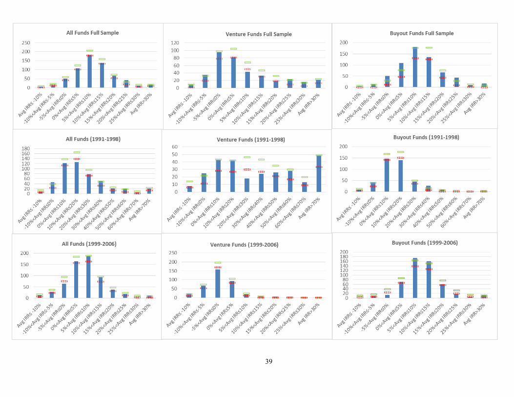
39

40

Figure 3. Frequency Distribution of Average Equal-Weighted IRR

The graphs show the frequency distributions of LPs’ average equal-weighted IRR for all funds, venture funds, and buyout funds. LPs in

the actual and every bootstrapped sample are divided to 10 groups based on their average IRR (Avg IRR). Each column in the figures

represents the number of LPs in each Avg IRR group from the actual sample. The horizontal lines for each column show the 10% and

90% of the bootstrapped frequencies for the same group. For the full sample and 1999-2006 subsample period, Avg IRR groups are based

on increments of 5%. Due to higher returns from the earlier period, Avg IRR groups in the 1991-1998 subperiod are based on increments

of 10%.

41

42

Table 4. Bayesian Model Estimates of Differences in LP Skill

This table displays the results of the Bayesian models described in Section IV. Panel A shows

results for the full sample period, Panel B includes only funds with vintage years between 1991

and 1998, and Panel C includes only funds with vintage years between 1999 and 2006. Odd-

numbered columns are based on Model 1, in which adjusted returns are computed as in Equation

(3). These estimates pick up LPs’ abilities to select funds within a GP family. Even-numbered

columns are based on Model 2, which further adjusts returns by subtracting fund-specific errors in

addition to the other non-skill-related effects in Equation (3). σλ is the estimated standard deviation

of LP fixed effects, which is our measure of differential LP skill. σπ is the estimated standard

deviation of the fund-LP random effects. βLP (all) is the estimated common constant term for all LPs.

This parameter measures the difference in performance between the funds invested by our sample

LPs and the Preqin universe. We also estimated a separate version of the model that included LP-

type effects. βLP (endow), βLP (pension), and βLP (other) are the estimated constant terms for endowments,

pension funds, and all other LPs, respectively. Estimates of σλ and σπ in this version of the model

are nearly identical to the values already reported here for the model with a single intercept, so we

do not include them in the table. All estimates are IRRs with Bayesian standard errors reported

below the estimates in parentheses.

Panel A: Full Sample (1991-2006)

All Funds Buyout Funds Venture Funds

(1) (2) (3) (4) (5) (6)

σλ 0.032 0.030 0.027 0.032 0.050 0.035

b.s.e. (0.003) (0.004) (0.003) (0.005) (0.005) (0.006)

σπ 1.630 0.833 1.364 0.845 1.987 0.835

b.s.e. (0.033) (0.078) (0.049) (0.108) (0.046) (0.108)

βLP (all) 0.193 0.202 0.178 0.209 0.203 0.174

b.s.e. (0.096) (0.124) (0.118) (0.156) (0.138) (0.165)

βLP (endow) 0.361 0.301 0.193 0.293 0.547 0.285

b.s.e. (0.116) (0.144) (0.142) (0.185) (0.177) (0.194)

βLP (pension) 0.139 0.207 0.148 0.209 0.119 0.191

b.s.e. (0.109) (0.144) (0.128) (0.173) (0.156) (0.182)

βLP (other) 0.187 0.197 0.219 0.227 0.129 0.136

b.s.e. (0.091) (0.117) (0.115) (0.148) (0.134) (0.158)

Obs 12,037 12,037 7,548 7,548 4,489 4,489

No. of LPs 630 630 528 528 379 379

43

Panel B: 1991-1998 subperiod

All Funds Buyout Funds Venture Funds

(1) (2) (3) (4) (5) (6)

σλ 0.063 0.032 0.036 0.0326 0.111 0.041

b.s.e. (0.007) (0.004) (0.004) (0.005) (0.016) (0.007)

σπ 2.292 0.854 1.384 0.847 3.237 0.884

b.s.e. (0.091) (0.096) (0.085) (0.124) (0.141) (0.134)

βLP (all) 0.306 0.127 0.080 0.075 0.733 0.213

b.s.e. (0.141) (0.139) (0.156) (0.166) (0.239) (0.211)

βLP (endow) 0.879 0.251 0.087 0.103 1.776 0.412

b.s.e. (0.198) (0.161) (0.198) (0.191) (0.362) (0.250)

βLP (pension) 0.131 0.079 0.041 0.051 0.338 0.139

b.s.e. (0.165) (0.154) (0.175) (0.184) (0.299) (0.222)

βLP (other) 0.231 0.109 0.105 0.081 0.478 0.157

b.s.e. (0.147) (0.137) (0.162) (0.168) (0.270) (0.209)

Obs 3,046 3,046 1,970 1,970 1,076 1,076

No. of LPs 498 498 418 418 276 276

Panel C: 1999-2006 subperiod

All Funds Buyout Funds Venture Funds

(1) (2) (3) (4) (5) (6)

σλ 0.027 0.026 0.028 0.029 0.038 0.033

b.s.e. (0.002) (0.004) (0.003) (0.004) (0.004) (0.006)

σπ 1.271 0.806 1.335 0.808 1.175 0.833

b.s.e. (0.045) (0.082) (0.060) (0.111) (0.073) (0.117)

βLP (all) 0.126 0.199 0.189 0.254 0.042 0.163

b.s.e. (0.104) (0.126) (0.134) (0.165) (0.154) (0.170)

βLP (endow) 0.127 0.286 0.196 0.322 0.045 0.226

b.s.e. (0.135) (0.146) (0.181) (0.200) (0.183) (0.195)

βLP (pension) 0.102 0.227 0.152 0.237 0.000 0.197

b.s.e. (0.129) (0.147) (0.153) (0.183) (0.175) (0.190)

βLP (other) 0.150 0.202 0.209 0.244 0.059 0.126

b.s.e. (0.103) (0.119) (0.131) (0.158) (0.152) (0.164)

Obs 8,991 8,991 5,578 5,578 3,413 3,413

No. of LPs 626 626 525 525 377 377

44

Figure 4. IRR Contribution of Estimated Skill

The figure shows the distribution of estimated skill contribution to IRR. For each LP, we obtain a Bayesian estimate of λ and compute

the IRR equivalent (i.e. the skill contribution to IRR). We divide LPs to bins based on their estimated skill contribution to IRR and count

the number of LPs in each bin. The upper limit of each bin is shown on the x-axis. The frequency count for each bin is shown on top of

each bar. We highlight 20 LPs in the figure below. These are the largest LPs for which we have data and the largest university endowments

in 2015. The average Bayesian standard error for the highlighted LPs is approximately 2.7% IRR. Returns are adjusted for vintage-year

fixed effects, firm-time random effects, and fund specific errors (i.e., Model 2).

45

46

Table 5. Correlation Analysis of Estimated Skill and Returns

The table shows correlation analyses of estimated skill (average λ) and IRRs across models and

time periods for all LPs and within three LP types. Panel A shows rank correlations between

estimated λ from Models 1 and 2. Panel B shows Pearson’s correlation of estimated λ in each

model with IRR. Panel C shows rank correlations of LPs’ average IRR and estimated λ between

two subsample periods: 1991-1998 and 1999-2006. Column Avg IRR shows correlations for

average IRRs. Column Model 1 λ and Model 2 λ show correlations for estimated λ of Model 1 and

Model 2, respectively. ***, **, and * indicate significance at the 1%, 5%, and 10% levels, respectively.

Panel A: Rank correlations between λ from two models

Full Sample 1991-1998 1999-2006

Endowments 0.82*** 0.84*** 0.69***

Pensions 0.80*** 0.80*** 0.73***

Others 0.78*** 0.73*** 0.69***

All LPs 0.80*** 0.79*** 0.69***

Panel B: Pearson's correlation of λ with IRR

Full Sample 1991-1998 1999-2006

Model 1 Model 2 Model 1 Model 2 Model 1 Model 2

Endowment 0.78*** 0.70*** 0.81*** 0.74*** 0.63*** 0.44***

Pensions 0.68*** 0.53*** 0.77*** 0.66*** 0.59*** 0.38***

Others 0.78*** 0.66*** 0.78*** 0.56*** 0.73*** 0.62***

All LPs 0.752*** 0.640*** 0.79*** 0.64*** 0.67*** 0.51***

Panel C: Correlation analysis of Avg IRR and λ across subsample

periods

Avg IRR Model 1 λ Model 2 λ

Endowments -0.220** 0.13 0.62***

Pensions -0.103 0.22** 0.59***

Others 0.028 0.06 0.49***

All LPs -0.076* 0.109** 0.539***

47

Table 6. Tests of Persistence within Different LP Types

This table shows tests of the standard deviation of persistence within different LP types.

Persistence is measured as the percentages of times LPs’ returns fall in the top half of funds given

their vintage years and fund types. LPs are divided to endowments, pensions, and all other LPs.

For each LP type, standard deviations are computed for the actual sample and all bootstrapped

samples. Column Actual reports the standard deviation from the actual sample. Column Boot

reports the average standard deviation across 1,000 bootstrapped samples. Column % > Actual

shows the percentage of bootstrapped samples with standard deviations greater than that of the

actual sample. Statistically significant values, highlighted in bold, are those for which % > Actual

is less than 10% or greater than 90%.

LP Type

All Funds Venture Funds Buyout Funds

Actual Boot % >

Actual Actual Boot

% > Ac-

tual Actual Boot

% > Ac-

tual

Endowments 0.21 0.17 0.1% 0.22 0.18 0.4% 0.21 0.18 0.6%

Pensions 0.20 0.15 0.0% 0.21 0.16 0.0% 0.20 0.16 0.5%

Other LPs 0.21 0.18 0.0% 0.22 0.19 0.2% 0.20 0.19 4.9%

48

Table 7. Bayesian Estimates of Differential Skill Controlling for Private and Public LPs

This table displays the results of the Bayesian estimate of skill with five LP-type fixed effects:

Private endowments, public endowments, private pensions, public pensions and all other LPs for

the full sample period. σλ is the estimated standard deviation of LP fixed effects. βLP (Private Endow),

βLP (Public Endow), βLP (Private Pension), βLP (Public Pension) and βLP (other) are the estimated constant terms for

private endowments, public endowments, private pension funds, public pension funds, and all

other LPs, respectively. All results adjust for firm-time random effects and vintage-year fixed

effects. Odd-numbered columns are based on Model 1 and even-numbered columns are based on

Model 2. All estimates are IRRs with Bayesian standard errors reported below the estimates in

parentheses.

All Funds Buyout Funds Venture Funds

(1) (2) (3) (4) (5) (6)

σλ 0.031 0.029 0.028 0.031 0.047 0.033

b.s.e. (0.002) (0.004) (0.003) (0.005) (0.004) (0.006)

βLP (Private Endow) 0.389 0.300 0.187 0.292 0.639 0.305

b.s.e. (0.127) (0.152) (0.158) (0.193) (0.187) (0.204)

βLP (Public Endow) 0.231 0.240 0.175 0.227 0.281 0.221

b.s.e. (0.154) (0.159) (0.176) (0.193) (0.244) (0.223)

βLP (Private Pension) 0.075 0.156 0.052 0.117 0.128 0.227

b.s.e. (0.117) (0.128) (0.138) (0.155) (0.195) (0.189)

βLP (Public Pension) 0.155 0.216 0.167 0.223 0.107 0.165

b.s.e. (0.118) (0.153) (0.139) (0.176) (0.176) (0.203)

βLP (Other) 0.179 0.188 0.210 0.213 0.119 0.133

b.s.e. (0.093) (0.115) (0.114) (0.138) (0.136) (0.163)

Obs 12037 12037 7548 7548 4489 4489

No. of LPs 630 630 528 528 379 379

49

Table 8. Actual vs. Bootstrapped Persistence and Average Returns for First-Time Funds

This table shows comparisons of the distributions of LPs’ persistence and average returns between

the actual and bootstrapped samples for first-time funds only. Column Standard Deviation of

Persistence reports the standard deviations of LP persistence, measured as the percentages of times

LPs’ returns fall in the top half of funds given their vintage years and fund types. Column Standard

Deviation of Size-Weighted IRR reports the standard deviations of LPs’ averaged returns weighed

by the logarithm of fund size, and column Standard Deviation of Equal-Weighted IRR shows the

same standard deviations when each fund return is weighed equally. Due to the smaller sample

size, tests are only performed for the full sample period from 1991 to 2006. All other variables are

the same as those described in Table 2. Bold numbers indicate that the actual and bootstrapped

samples are significantly different, with % > Actual either smaller than 10% or greater than 90%.

Standard Deviation of

Persistence

Standard Deviation of

Size-Weighted IRR

Standard Deviation

Equal-Weighted IRR

Actual Boot

% >

Actual Actual Boot

% > Ac-

tual Actual Boot

% >

Actual

All funds 0.26 0.26 33.9% 14.28 14.58 53.5% 15.1 15.36 50.2%

Venture funds 0.28 0.27 4.8% 28.12 23.21 3.6% 29.12 24.8 8.0%

Buyout funds 0.28 0.26 5.3% 9.61 9.92 71.3% 9.5 9.91 75.8%

50

Table 9. Bayesian Model Estimates of Differential Skill Using First-Time Funds

This table displays the results of the Bayesian estimates of differential LP skill using their

investments in first-time funds in the full sample (1991-2006). The estimation follows the

Bayesian model described in Section IV. All variables are defined in Table 4. Odd-numbered

columns do not adjust for fund-specific errors in Equation (3) (i.e., Model 1). Even-numbered

columns do perform this adjustment (i.e., Model 2). βLP (endow), βLP (pension), and βLP (other) are estimated

in a separate Bayesian regression from the other listed parameters. All estimates are IRRs with

Bayesian standard errors reported below the estimates in parentheses.

All Funds Buyout Funds Venture Funds

(1) (2) (3) (4) (5) (6)

σλ 0.038 0.025 0.036 0.028 0.058 0.031

b.s.e. (0.004) (0.002) (0.003) (0.003) (0.009) (0.003)

σπ 1.915 0.894 1.437 0.922 2.532 0.845

b.s.e. (0.052) (0.097) (0.068) (0.137) (0.098) (0.106)

βLP (all) -0.002 0.005 0.089 0.036 -0.136 -0.035

b.s.e. (0.090) (0.084) (0.110) (0.116) (0.145) (0.117)

βLP (endow) 0.126 0.051 0.105 0.083 0.120 -0.003

b.s.e. (0.157) (0.124) (0.174) (0.171) (0.278) (0.172)

βLP (pension) -0.114 -0.019 0.020 0.005 -0.454 -0.088

b.s.e. (0.117) (0.102) (0.129) (0.128) (0.222) (0.140)

βLP (other) 0.046 0.019 0.124 0.043 -0.068 -0.023

b.s.e. (0.098) (0.091) (0.120) (0.124) (0.168) (0.126)

Obs 2,470 2,470 1,582 1,582 888 888

No. of LPs 539 539 448 448 318 318

51

Appendix 1

The regression model (step 2) is

𝑦𝑖𝑢�̂� = 𝑋𝐿𝑃𝑗𝛽𝐿𝑃 + 10𝜆𝑗 + π𝑖𝑢𝑗

Where 𝑦𝑖𝑢�̂�is the return of Limited Partner j’s investment in the uth fund of the ith PE firm adjusted

for firm-time random effects and demeaned at the vintage year level:

𝑦𝑖�̂� = 𝑦𝑖𝑢 − 𝑋𝑖𝑢𝛽 − ∑ 𝜂𝑖𝜏

𝑡𝑖𝑢+9

𝜏= 𝑡𝑖𝑢

Definitions

The parameter vector we want to estimate is 𝜃𝐿𝑃 ≡ (𝛽𝐿𝑃, 𝜎𝜆2, 𝜎𝜋

2).

Let 𝑈𝑗𝐿𝑃be the number of PE investments made by Limited Partner j, let 𝑈𝐿𝑃 = ∑ 𝑈𝑗

𝐿𝑃𝑗 , and let

𝑁𝐿𝑃 be the number of LPs in the sample.

𝑋𝐿𝑃 is a𝑈𝐿𝑃 × 1 vector or a 𝑈𝐿𝑃 × 3 matrix that contain either a single intercept or a LP category

(endowment, pension fund, other) indicator, respectively.

𝐿 is a 𝑈𝐿𝑃 × 𝑁𝐿𝑃 matrix where each row represent a LP-fund return pair and each column

represents a LP. Each row contains an indicator which is equal to 10 in the column of the

corresponding LP.

A1 LP (random) effects

We sample the LP effects, 𝜆𝑗,using a Bayesian regression. The prior is

𝜆𝑗 ~ 𝒩(0, 𝜎𝜆2)

The posterior from which we sample is

𝜆𝑗|{𝑦𝑖�̂�}, 𝜃𝐿𝑃, 𝑑𝑎𝑡𝑎 ~ 𝒩(𝜇𝜆, 𝜎𝜋2𝐵−1)

where

𝐵 =𝜎𝜋

2

𝜎𝜆2 𝕀𝑁𝐿𝑃 + 𝐿′𝐿

𝜇𝜆 = 𝐵−1(𝐿′(�̂� − 𝑋𝐿𝑃𝛽𝐿𝑃))

A2 Variance of error term and βLP coefficient

In this step we condition on the latent variables {𝜆𝑗} sampled in the previous step. With the

conjugate prior

52

𝜎𝜋2 ~ 𝐼𝒢(𝑜0, 𝑝0)

𝛽𝐿𝑃|𝜎𝜋2 ~ 𝒩(𝜇𝐿𝑃0

, 𝜎𝜋2Σ𝐿𝑃0

−1 )

the posterior distribution is

𝜎𝜋2|{𝜆𝑗}, 𝑑𝑎𝑡𝑎 ~ 𝐼𝒢(𝑜, 𝑝)

𝛽𝐿𝑃|𝜎𝜋2, {𝜆𝑗}, 𝑑𝑎𝑡𝑎 ~ 𝒩(𝜇𝐿𝑃 , 𝜎𝜋

2Σ𝐿𝑃−1)

where

𝑜 = 𝑜0 + 𝑈𝐿𝑃

𝑝 = 𝑝0 + (�̂� − 𝐿𝜆 − 𝑋𝐿𝑃𝛽𝐿𝑃)′(�̂� − 𝐿𝜆 − 𝑋𝐿𝑃𝛽𝐿𝑃) + (𝜇𝐿𝑃 − 𝜇𝐿𝑃0

)′Σ𝐿𝑃0(𝜇𝐿𝑃 − 𝜇𝐿𝑃0

)

Σ𝐿𝑃 = Σ𝐿𝑃0+ 𝑋𝐿𝑃′𝑋𝐿𝑃

𝜇𝐿𝑃 = Σ𝐿𝑃−1(Σ𝐿𝑃0

𝜇𝐿𝑃0+ 𝑋𝐿𝑃

′ (�̂� − 𝐿𝜆))

A3 Variance of LP effects

Using the inverse gamma prior

𝜎𝜆2 ~ 𝐼𝒢(𝑙0, 𝑚0)

the posterior distribution from which we sample is

𝜎𝜆2|{𝜆𝑗}, 𝑑𝑎𝑡𝑎 ~ 𝐼𝒢(𝑙, 𝑚)

where

𝑙 = 𝑙0 + 𝑁𝐿𝑃

𝑚 = 𝑚0 + 𝜆′𝜆

A4 Priors and starting values

We use diffuse priors for all the parameters in the LP model. For the variance of the error term, we

set 𝑜0 = 2.1 and 𝑝0 = 1. For the variance of the LP effects, we set 𝑙0 = 2.1 and 𝑚0 = 0.152. For

the beta coefficients, we set Σ𝐿𝑃0 equal to the identity matrix and 𝜇𝐿𝑃0

equal to 0 (or to a zero-

valued vector for the case of LP category β). We initialize all the variables at their prior means. We

do not need starting values for the LP effects since they are the first variables we simulate. The

choice of the priors is in the spirit of section A7 in the KS appendix.

53

Appendix 2: Skill Estimates of Individual LPs

The table shows the IRR equivalent of estimated 𝜆𝑗 for each LP. Results are adjusted for vintage-year fixed effects, firm-time random effects, and fund

specific errors. Bayesian estimates of 𝜆𝑗 are transformed to IRR using 𝑒 𝜆𝑗 − 1. For each LP, Column λ shows the IRR equivalent of the average λ

across all MCMC cycles. Column Standard Error is the IRR equivalent of Bayesian standard error for 𝜆𝑗.

LP Name λ Standard Error LP Name λ Standard Error LP Name λ Standard Error

3i Group -0.46% 2.69% Allianz 0.33% 2.59% AT&T -0.76% 2.72%

3M -1.18% 2.95% Allianz Capital Partners 0.69% 3.01% ATP PE Partners -0.38% 2.28%

747 Capital 2.88% 3.28% Allstate Insurance -1.21% 2.83% Auda Private Equity -0.33% 2.01%

AA Capital Partners 0.34% 3.01% Alpha Associates -0.69% 2.35% Avadis Anlagestiftung -0.51% 1.85%

ABB Group Investment 0.26% 3.10% AlpInvest Partners 0.48% 2.33% Avery Dennison -1.64% 2.74%

Abbey National Financial 0.59% 2.90% Altira Heliad Mgmt 0.59% 2.97% Aviva International Ins 1.72% 3.54%

Abbey National Treasury 0.58% 2.70% Amanda Capital 1.09% 2.53% Aviva Investors Global 0.24% 2.80%

Abbott Capital Mgmt 1.38% 1.98% AmBex Venture Group 2.32% 3.37% AXA -0.11% 2.58%

Abu Dhabi Invest Authority 1.39% 3.38% American Beacon Advisors -0.56% 2.72% AXA Financial 1.20% 3.36%

Access Capital Partners -0.78% 2.85% American Family Insurance -0.81% 2.75% Ardian 0.15% 2.52%

Adams Street Partners -0.83% 2.15% American International -0.23% 2.91% Bahrain Middle East Bank 1.72% 3.51%

Adveq Mgmt -1.12% 2.33% American PE Partners -0.92% 2.65% BAML Capital Partners -0.86% 2.11%

Aegon USA Investment Mgmt 0.71% 2.99% Ameritech -1.37% 2.45% BancBoston Investments 1.04% 2.28%

Aetna Investment Arm -0.88% 2.45% Amherst College 2.73% 2.46% Bank Gutmann 0.68% 2.75%

Aetna Life Insurance 0.49% 3.15% AMR Investment Services -0.89% 2.59% Bank Leumi -0.42% 2.82%

AIG Global Investment -0.45% 2.30% Andrew W. Mellon FDN 1.71% 2.40% Bank of America -1.02% 2.35%

Akina -0.13% 2.95% Antares Capital -0.39% 2.23% Bank of America Merrill Lynch 0.70% 3.00%

Alaska Permanent Fund 1.05% 1.94% Aon Advisors -0.70% 2.81% Bank of New York Mellon -2.23% 2.87%

Alaska Retirement Mgmt Board 0.71% 2.87% Aon Group -0.55% 3.36% Bank Of Nova Scotia -1.01% 2.79%

Alaska State Pension 1.61% 1.82% AP Fonden 2 0.67% 2.67% Bank One Capital Markets -1.28% 2.80%

Alcoa -0.95% 2.73% APEN AG 0.50% 2.17% Bank Vontobel -0.65% 2.38%

Alfred I. duPont Testamentary 0.28% 2.17% APG Asset Mgmt US -0.25% 2.90% Barclays Bank -1.02% 2.35%

Alfred P. Sloan Foundation 0.41% 2.93% Arizona State Retirement 0.93% 2.77% Baxter International 0.42% 3.00%

All State Venture Capital 1.11% 3.00% Arkansas TRS -0.50% 2.74% Bayer -0.49% 2.44%

AllianceBernstein 1.50% 3.10% Arle Capital Partners -1.68% 3.41% BC Investment Mgmt -0.15% 2.52%

54

LP Name λ Standard Error LP Name λ Standard Error LP Name λ Standard Error

BDC Venture Capital -2.76% 3.44% Carnegie Mellon University 0.36% 2.59% Commercial Union Ins 0.14% 2.95%

Bear Stearns -0.06% 2.89% Carolina Power & Light -0.17% 3.03% Commonfund Capital -0.23% 1.97%

Belmont Global Advisors 0.35% 2.96% Case Western Reserve Univ 0.60% 2.96% Commonwealth Fund -0.23% 1.97%

Berea College 3.73% 3.40% Catholic Charities Chicago 0.16% 3.31% Connecticut State Retire -1.15% 2.10%

Bessemer Invest Mgmt -0.62% 2.15% Caxton Associates -0.37% 3.35% Conversus Capital -0.18% 1.65%

BHF-Bank 1.66% 3.52% Cazenove Capital Mgmt 0.75% 2.70% Cornell University 1.73% 2.03%

Bio*One Capital -1.06% 3.04% CDC Group -1.38% 2.82% Corning 1.16% 2.83%

BIP Investment Partners 0.09% 3.10% CDPQ 0.44% 2.87% Covera Ventures -1.29% 3.15%

BlackRock -1.44% 2.87% Charles Schwab Group -0.86% 2.85% CPP Investment Board -1.05% 2.28%

BMO Capital 0.01% 3.03% Charles Schwab Bank 0.04% 2.99% Cramer Rosenthal McGlynn -1.06% 2.92%

Bmp 0.32% 2.64% Chrysler Master Retire -1.68% 2.32% Credit Agricole -0.93% 2.95%

Boeing -1.15% 2.49% Church Pension Fund 0.22% 2.55% Credit Suisse -0.36% 2.63%

Bombardier Pension 0.98% 3.43% CIBC -0.20% 2.89% CSFB Private Equity -1.52% 2.14%

Bowdoin College 0.83% 3.13% Cincinnati Bell 1.21% 3.29% CSGN -1.66% 2.54%

BP America -0.89% 3.19% Cisco Systems 2.40% 3.01% Customized Fund Investment -1.15% 2.72%

BP Pension -0.18% 2.85% Citi -0.05% 2.15% Cuyahoga Capital Partners 1.37% 3.26%

Bramdean Asset Mgmt 0.63% 3.09% Citigroup Private Equity -0.62% 2.33% Daimler 1.62% 3.03%

Brinson Partners -0.08% 2.64% City of Boston Retirement -0.84% 2.66% Daiwa Corporate Invest -0.98% 3.07%

Bristol-Myers Squibb 0.49% 1.84% City of Philadelphia -0.45% 2.89% Danske Bank 1.83% 3.14%

Brown Brothers Harriman 0.20% 2.71% City of Worcester Retirement 0.51% 3.04% Danske Private Equity -0.51% 2.36%

Brown University -0.98% 2.85% Clal Industries and Investments 1.43% 3.07% Dartmouth College 3.03% 2.30%

Buckeye Venture Partners 0.31% 2.80% Claude Worthington Benedum -0.11% 2.77% Davidson College 2.18% 3.47%

Bure Equity 1.28% 3.42% Cleveland Foundation 1.33% 3.32% Dayton Power and Light 0.66% 3.12%

Cal Tech 1.05% 2.35% CMS Fund Advisers 0.85% 2.00% DeA Capital 0.34% 2.17%

CalPERS -1.23% 1.56% CNA Financial -0.51% 3.37% Deere & Company -0.92% 2.80%

CalSTRS 0.08% 1.61% CNP 0.25% 2.94% Delaware State Board Pension 2.18% 3.19%

Cambridge Retirement -0.69% 2.51% Colby College 1.57% 2.77% Delta Air Lines -2.66% 2.83%

CIBC World Markets -0.20% 2.89% Colgate University 1.66% 2.79% Denison University 0.87% 3.08%

Capital Access Funds -2.06% 2.79% Colorado PERA -1.92% 1.91% Denver PSR -1.20% 2.59%

Capvent -1.00% 2.77% Columbia University 1.80% 2.59% Deutsche Bank Alex. Brown 0.01% 3.01%

Carleton College 1.74% 2.91% Commercial Union Ins 0.14% 2.95% Deutsche Bank Trust Corp -0.03% 2.91%

55

LP Name λ Standard Error LP Name λ Standard Error LP Name λ Standard Error

Deutsche Beteiligungs 0.46% 3.13% Fire & Police San Antonio -0.97% 3.08% Grove Street Advisors -0.53% 1.98%

District of Columbia Retire -1.05% 2.99% First Chicago Investment -0.58% 2.77% Grupo Guayacan 1.44% 2.01%

DKA Capital -2.57% 3.36% FLAG Capital Mgmt -0.32% 2.15% GTE Investment Mgmt -0.65% 3.12%

DLJ Merchant Banking Part -1.84% 2.77% Fleet Equity Partners -0.36% 2.75% Halyard Capital -0.71% 2.80%

Dow Chemical -1.97% 2.65% Florida State Board of Admin -0.62% 2.21% Hamilton Lane (Singapore) 0.56% 2.90%

DSM Venturing -0.30% 3.05% Fondinvest Capital -0.68% 2.75% Hamilton Lane Advisors -0.04% 1.96%

Duke Power 2.30% 3.44% Ford Foundation 1.51% 2.03% Harald Quandt Holding 0.77% 3.21%

Duke University 0.77% 1.86% Ford Motor -0.44% 3.12% HarbourVest Partners -0.29% 2.04%

Dunedin Capital Partners 1.87% 3.43% Fort Washington Capital 0.72% 1.95% Harvard University 0.70% 2.05%

DuPont Capital Mgmt -1.45% 2.87% FPPA Colorado -0.13% 1.95% Heller Financial -0.63% 2.54%

Duquesne Light 0.34% 3.04% Frank Russell -0.12% 2.95% Hellman & Friedman 1.27% 3.29%

E.I. DuPont De Nemours 0.74% 2.53% Fresno County ERA -0.84% 3.04% Henderson Equity Partners -0.72% 2.54%

EDS Retirement 1.26% 2.62% GE Asset Mgmt -0.02% 2.66% Henry J. Kaiser Family FDN -0.47% 2.67%

EES Acquisition Fund II 0.88% 2.81% GE Global Sponsor Finance 0.13% 2.91% Henry Luce Foundation 0.09% 3.37%

Electricite de France -1.41% 3.22% General American Investors -1.38% 3.26% Hewlett-Packard 0.61% 2.77%

Electrolux -0.90% 3.19% General Electric -1.56% 2.56% HFRRF -0.68% 2.93%

Eli Lilly 0.62% 3.19% General Mills -0.41% 2.75% Hillman Company -2.23% 2.81%

Emory University -0.49% 2.88% Georgia Tech 1.46% 2.95% Hillman Foundation -0.21% 3.00%

Equitrust -1.05% 2.60% GIC Special Investments 0.36% 2.01% HLM Venture Partners -1.11% 3.40%

ERS Hawaii 0.46% 2.70% GIMV -1.74% 2.87% Hoffmann-La Roche 0.90% 2.87%

ERS Texas -1.05% 2.60% Goldman Sachs Asset Mgmt -1.93% 2.41% Horsley Bridge Partners 2.50% 2.16%

ERS RI 1.92% 3.24% Goldman Sachs Merch Bank -0.96% 2.36% Hospitals of Ontario Pension -0.51% 2.88%

Eurazeo -0.38% 2.72% Goldman Sachs PE Group 0.58% 2.60% Houston HMEPS -1.68% 2.95%

eValue Europe -1.32% 2.89% Goodyear -1.82% 2.96% Houston Police Pension -0.04% 1.93%

Evangelical Lutheran Church 2.01% 2.80% Gov of Singapore Invest -0.43% 2.55% Howard Hughes Med. Inst. -0.35% 2.08%

Ewing M. Kauffman FDN -0.23% 2.29% Granite Hall Partners 0.69% 2.78% HRJ Capital -0.73% 2.83%

Exxon 0.23% 2.93% Graphite Capital Mgmt 0.62% 2.65% HSBC France 1.69% 3.53%

F & C Private Equity Trust -2.02% 2.81% Greater Manchester Pension 1.28% 3.10% IBM Retirement 1.34% 2.29%

F & C Asset Mgmt -0.44% 2.73% Greenspring Associates 1.36% 2.24% IDInvest Partners -1.65% 2.78%

FFP 0.08% 2.96% Groupama Private Equity 0.34% 2.37% Illinois Municipal Retire 0.01% 1.60%

Finnish Industry Investment 1.52% 2.80% Groupe IDI 0.05% 2.97% Illinois State Board of Invest -1.20% 2.27%

56

LP Name λ Standard Error LP Name λ Standard Error LP Name λ Standard Error

ID Holding Partners -0.13% 2.46% KeyCorp 0.24% 2.75% Massachusetts Mutual Life -0.33% 2.68%

Indiana PRS 1.39% 1.78% KKR PEI Investments -0.18% 3.10% Massachusetts PRIT 0.08% 2.00%

Indiana University -1.72% 2.83% Knightsbridge Advisers 2.70% 2.82% Mayo Foundation -1.79% 2.43%

ING Investment Mgmt -0.39% 2.92% König & Cie 0.15% 2.74% MBTA -0.62% 2.37%

International Finance -1.16% 2.79% Koor Corporate Venture Capital -0.62% 3.06% MC Financial Services -0.89% 3.04%

Invesco Advisers -0.76% 2.85% Kresge Foundation 0.65% 2.69% MD Dept of Bus and Econ Dvlpmnt -1.66% 2.98%

Investco Private Capital 1.25% 2.04% Kuwait Financial Private Equity 0.35% 2.08% Mead -2.08% 3.09%

Invest Fund for Foundations 1.26% 2.34% Kuwait Investment Authority 0.87% 2.66% Meadows Foundation -1.63% 2.21%

Iowa PERS 1.03% 1.90% LA City Employees' Retirement 0.31% 2.20% Merrill Lynch Ventures 0.90% 3.16%

ITAA Retirement -0.31% 2.03% LA County Employees' Retire 0.60% 1.91% MERS of Michigan 0.05% 2.49%

Itochu -0.59% 3.03% LA Fire & Police Pension 0.44% 2.08% Mesirow Financial Hld 1.14% 2.85%

Itochu Tech Venture Investment -0.57% 2.93% Landmark Partners -0.52% 2.61% Metropolitan Life Ins -0.20% 2.43%

J. Paul Getty Trust 1.25% 3.21% Länsförsäkringar 1.61% 3.23% Metropolitan Museum of Art 1.91% 2.91%

J.F. Shea 1.93% 2.96% Lehman Brothers PE 0.95% 2.54% Meyer Memorial Trust -0.92% 2.78%

J.P. Morgan Asset Mgmt -0.13% 2.08% Lexington Partners -0.43% 2.63% MIC Capital -0.51% 3.10%

J.P. Morgan Partners -1.40% 2.03% LGT Capital Partners 0.70% 2.08% Michelin North America -1.80% 2.41%

JAFCO -0.84% 2.86% Liberty Mutual Holding 0.46% 1.87% Michigan Dept of Treasury 0.47% 1.93%

James Irvine Foundation 0.19% 2.89% Liberty Mutual Insurance 0.66% 1.91% Michigan State University 2.75% 3.49%

J.D. & C.T. MacArthur FDN 0.28% 2.73% Lifespan -0.24% 2.85% Middlebury College 0.00% 2.88%

John A. Hartford FDN 2.84% 3.51% Lincoln National -0.68% 3.04% Minnesota Mutual Life Ins -2.98% 2.94%

John Deere Pension -0.86% 2.91% LMS Capital -0.60% 2.66% Minnesota Board of Invest -0.81% 2.05%

John Hancock Life Insurance 0.63% 2.82% Lockheed Martin 0.71% 2.99% Missouri PSRS 1.05% 2.63%

John S. & James Knight FDN -0.08% 2.73% Louisiana SERS 1.69% 1.96% Missouri MOSERS -0.19% 2.96%

Johnson & Johnson -1.29% 2.62% Lucent Technologies -1.34% 2.76% MIT 1.17% 2.03%

JPMP Capital -1.82% 2.25% Lynde & Harry Bradley FDN -1.41% 2.96% MITIMCo Private Equity 0.12% 2.36%

K & E Partners 0.02% 3.19% M.J. Murdock Charitable Trust 4.30% 3.28% Mitsui & Co. (USA) 0.12% 2.36%

Kansas PERS -0.32% 1.97% Macquarie Private Capital 0.26% 2.94% Mitsui & Co. -1.72% 2.80%

KBC -1.73% 3.04% Madison Dearborn Partners 0.41% 3.21% Montana Board of Invest -0.68% 2.35%

Kenmont Capital Partners -0.08% 2.88% Martin Currie Investment Mgmt -0.58% 2.84% Montreal Police Pension -0.61% 2.89%

Kentucky Retire Systems -0.10% 2.86% Maryland SRPS 0.75% 2.79% Morgan Stanley -0.71% 2.77%

Kenyon College -1.48% 2.43% Masco 0.02% 3.06% Morgan Stanley Alt Invest 0.57% 2.73%

57

LP Name λ Standard Error LP Name λ Standard Error LP Name λ Standard Error

Mousse Partners 0.54% 2.94% Northwestern University -1.09% 2.11% Pantheon Ventures -0.61% 2.05%

MPC Münch. Petersen A. 0.06% 2.99% Notre Dame Endowment 2.73% 2.08% Parallel Private Equity 0.01% 3.04%

Mutual of NY Life Ins 0.05% 2.49% Novartis Vaccines & Diag. -0.91% 3.02% Parish Capital Advisors -1.11% 2.89%

Mutual of Omaha Insurance -1.19% 2.56% NPRF (Ireland) 1.49% 2.75% Park Street Capital -0.09% 1.90%

National City Bank 1.35% 3.18% NY City Police Pension -0.05% 2.97% Partners Group Holding 0.29% 2.39%

National City Equity Part 0.66% 2.18% NY City Retirement -1.10% 2.05% Pathway Capital Mgmt 0.10% 1.98%

National Grid -1.16% 2.51% NY Common Retirrement Fund -0.27% 1.90% Paul Capital France -0.99% 3.04%

Nationwide -1.49% 2.16% NY Life Capital Partners -0.26% 2.35% Paul Capital Partners -0.30% 2.61%

Natixis Private Equity -0.51% 3.03% NY STRS 1.07% 2.08% Penn Mutual Life Insurance -0.97% 2.63%

Nautic Partners 0.54% 2.56% NYS OSC 0.06% 2.59% Pennsylvania State University 0.83% 2.93%

NB Alternatives Advisers 1.26% 2.10% Oberlin College 0.83% 2.95% Peppertree Capital Mgmt 0.09% 2.74%

NB Private Equity Partners 0.29% 2.44% OCERS -0.97% 2.22% Peppertree Partners 0.67% 2.36%

Nestle 1.27% 2.66% Ohio OBWC -1.68% 2.37% Performance Equity Mgmt 1.20% 2.91%

Neuberger Berman 0.32% 2.63% Ohio Capital Fund 0.80% 2.85% PERS Colorado -0.60% 2.09%

Nevada PERS 0.72% 2.83% Ohio Carpenters H & W 0.90% 3.13% PERSI Idaho 0.39% 2.96%

New Hampshire Retirement -2.03% 2.35% Ohio Police & Fire Pension -2.28% 2.42% Pew Charitable Trusts -0.97% 2.81%

New Jersey Division of Invest -0.08% 2.53% Ohio State University -0.56% 2.98% Pfizer 0.13% 2.31%

New Mexico Edu Retire. Board 0.22% 2.77% Oklahoma Capital Invest Board -1.27% 3.04% PGGM 0.83% 2.56%

New Mexico St Invest Counc. -0.60% 1.81% Olayan Group 0.56% 3.14% Philadelphia Pension 0.40% 2.21%

New York Life Insurance -0.05% 2.97% OMERS 0.52% 2.98% Phillips Academy 2.83% 3.52%

NIB Capital Private Equity -1.10% 2.05% Ontario Teachers' Pension -0.50% 2.19% Phoenix Life Insurance -1.65% 2.14%

NIBC Holding -0.26% 2.35% OPERS -0.04% 2.01% PNC Equity Partners -1.14% 2.17%

Nippon Venture Capital -0.54% 2.29% OPPRS -1.69% 2.98% Pohjola Bank 1.82% 3.19%

North Sky Capital 0.56% 2.42% Oregon PERS -0.55% 1.93% Pomona Capital 0.44% 2.03%

Northeastern University 3.47% 2.74% Oregon State Treasury -0.30% 2.08% Pomona College 1.98% 2.47%

Northleaf Capital Partners 1.13% 2.54% ORS Michigan -1.08% 2.35% Portfolio Advisors 0.27% 1.85%

Northrop Grumman -0.90% 3.17% Owens-Illinois 1.42% 3.05% PPM America -0.71% 2.81%

Northwestern Insurance -0.29% 2.75% PA Employees' Retirement -1.29% 1.89% Princess Mgmt 0.10% 1.94%

Northwestern Invest Mgmt -0.20% 2.11% Pacific Life Insurance 0.50% 2.79% Princess Private Equity 0.52% 1.89%

Northwestern Memorial Hosp 1.15% 2.14% PacifiCorp -0.76% 1.84% Princeton University -0.12% 2.18%

Northwestern Mutual Life 0.18% 2.16% Pamlico Capital -1.90% 2.68% Private Advisors 0.72% 2.94%

58

LP Name λ Standard Error LP Name λ Standard Error LP Name λ Standard Error

Progress Energy -0.15% 3.05% Sal. Oppenheim jr. & Cie. 0.48% 2.00% Starling International Mgmt 0.46% 2.76%

Progress Investment Mgmt -2.37% 3.11% Santander UK -0.42% 2.95% State Farm Life 1.72% 3.55%

Promark Global Advisors 1.10% 1.86% SBC Communications -0.09% 2.72% State Farm Mutual Auto 0.41% 3.24%

Promark Invest Advisors -0.17% 2.21% Scottish Investment Trust -1.04% 2.97% State of WI Invest Board -0.88% 1.78%

Providence Employees' Retire 0.17% 2.83% Scottish Widows Investment -0.99% 2.65% Stichting Pensioenfonds 1.54% 3.02%

Provident Bank 1.93% 3.76% SDCERA 0.49% 2.18% Stonehenge Partners 0.01% 3.18%

Prudential Insurance 0.58% 2.69% Sears Investment Mgmt 1.38% 2.86% Strategic Investment Solutions -1.24% 2.26%

PSEG Resources -0.27% 3.30% SEB Asset Mgmt -0.24% 2.64% STRS Ohio -1.43% 1.97%

PSPRS AZ 0.97% 2.84% SERS Ohio -1.24% 2.21% Sun Life Financial -1.27% 2.97%

Public Service Enterprise 1.94% 3.12% SF City and County Retire 0.36% 2.50% SunAmerica Ventures -1.30% 2.64%

Pyxis Capital -0.39% 2.67% SFERS 1.55% 2.15% SunTrust Banks -0.28% 2.91%

Qwest Asset Mgmt -1.28% 2.81% SGAM Alternative Invest -0.20% 3.22% SURS Illinois -0.32% 2.02%

RBC Venture Partners 0.30% 3.10% ShaPE Capital 0.73% 2.24% SVB Capital 2.20% 2.44%

RCP Advisors 1.02% 2.65% Shell Oil -0.50% 2.92% SVB Financial Group -0.86% 2.83%

RDV -1.38% 3.01% Sherman Fairchild FDN -0.29% 2.97% SVB Silicon Valley Bank -0.67% 2.80%

Rensselaer Polytech Institute -1.00% 2.65% Siemens Venture Capital 0.27% 2.73% SVG Advisers 0.17% 2.85%

Rho Capital Partners 0.92% 3.25% Siguler Guff 0.52% 1.86% SVG Capital 1.01% 2.09%

RI Treasury 0.22% 2.14% SilverHaze Partners -0.15% 2.80% Swarthmore College -1.38% 2.88%

Richard King Mellon FDN -0.79% 3.00% Sitra Investment Arm 0.32% 2.54% SIFEM 0.05% 2.84%

Riverside Church -2.30% 3.03% Sjätte AP 1.29% 3.44% Swiss Life Private Equity 0.26% 2.70%

Robeco Group -0.14% 2.13% Skandia Liv Asset Mgmt 0.68% 2.82% Swiss Re Private Equity 0.25% 2.00%

Robert Wood Johnson FDN 1.18% 2.69% SL Capital Partners 0.94% 2.15% Swiss Reinsurance -2.49% 2.70%

Rockefeller Br. Fund -0.21% 2.89% Source Capital Group 2.34% 3.45% TA Associates 0.67% 2.96%

Rockefeller Fam Trust 1.78% 2.95% South Carolina Retirement 0.52% 2.80% TD Capital 0.80% 2.27%

Rockefeller University 0.61% 2.57% South Dakota Invest Counc. -0.39% 2.70% Teachers' Private Capital -0.32% 2.61%

RogersCasey 0.41% 2.44% Southern Company -1.44% 3.07% Temasek Capital -0.65% 2.60%

Royal Bank of Canada Capital 0.23% 2.92% Spelman College 1.36% 3.32% Texas A&M 1.51% 3.73%

Rush University Med Center -0.75% 2.97% SR One -2.04% 2.86% Textron -2.05% 3.01%

RWB RenditeWertBeteiligung -0.29% 2.39% St. Paul Venture -0.46% 2.83% The Glenmede Trust Co 0.71% 1.87%

S. C. Johnson & Son -0.79% 2.97% Standard Life -1.80% 2.45% The GS Group -0.43% 2.58%

Safeguard Scientifics -1.66% 3.26% Stanford University 1.00% 2.17% The Key Corporation 1.39% 3.29%

59

LP Name λ Standard Error LP Name λ Standard Error LP Name λ Standard Error

Thomas Weisel Capital

Mgmt 0.85% 2.38%

United Technologies -0.21% 2.27%

Virginia Tech -0.95% 2.80%

Thrivent Financial Lutherans -0.41% 3.05% University of California -1.16% 2.09% Vontobel Holding 0.23% 3.11%

TIAA-CREF Invest Mgmt -0.22% 3.07% University of Chicago 0.21% 2.81% Vulcan Capital -1.10% 2.78%

TIF Ventures 0.33% 2.77% University Of Colorado -1.16% 2.65% Vulcan Materials 0.99% 3.21%

Time Warner -0.67% 3.08% University of Michigan 1.11% 1.96% W.K. Kellogg Foundation -0.63% 3.12%

Tokio Marine & Nichido

Fire Ins 2.09% 3.29% University of Minnesota 2.23% 2.77%

Wachovia 0.12% 2.95%

Toronto-Dominion Bank 0.16% 2.94% University of North Carolina -1.98% 2.16% Walt Disney 1.98% 3.08%

Travelers Insurance -0.65% 3.04% University of Pennsylvania 0.94% 2.79% Washington State Invest Board -0.20% 1.70%

Tredegar -2.70% 2.77% University of Pittsburgh -0.30% 2.20% Washington University -0.54% 1.95%

Tri-State Ventures -1.40% 2.86% University of Richmond -1.66% 2.67% Wellesley College -1.73% 2.16%

Triton Systems 2.53% 3.56% University of Texas -0.82% 1.76% Weome Trust 1.32% 2.97%

TRS Illinois -2.19% 1.98% University of Toronto 0.71% 2.93% Wesleyan University -0.02% 2.97%

TRS Louisiana -0.28% 2.28% University of Virginia 0.43% 2.47% West Midlands Pension 1.45% 2.90%

TRS texas 0.97% 1.92% University of Washington 1.82% 2.22% West Yorkshire Pension -1.25% 3.02%

Trust Plan -2.61% 2.76% University Of Wisconsin 0.14% 3.03% WestLB Private Equity 0.19% 2.75%

Tunisie Leasing -0.73% 3.12% USC 0.60% 2.63% William & Flora Hewlett FDN 3.60% 2.49%

Twin Bridge Capital Partners -0.87% 2.80% Utah Capital Investment -0.85% 2.77% Williams College 0.65% 2.78%

U.S. Bancorp -0.25% 2.91% Utah Retirement Systems 0.68% 1.97% Wilshire Associates -1.15% 1.92%

U.S. Steel & Carnegie

Pension 0.09% 2.89% Vanderbilt University 1.21% 2.58%

Wilton Asset Mgmt -0.60% 2.74%

U.S. West Investment Mgmt 0.34% 3.08% Vassar College -0.15% 3.02% Wisconsin Alumni Research FDN -1.87% 2.49%

UBS Capital 0.69% 3.05% VenCap International 2.89% 2.42% World Bank Group 0.15% 2.84%

UMWA Health & Retire -0.18% 2.44% Verizon Communications 0.56% 2.78% Y.M.C.A. Retirement Fund -0.72% 2.04%

Unisys 0.40% 2.05% Virginia Retirement System 0.88% 1.97% Yale University 0.17% 2.06%

Thomas Weisel Capital

Mgmt 0.85% 2.38%

United Technologies -0.21% 2.27%

Virginia Tech -0.95% 2.80%