measuring knowledge spillovers: a non-appropriable …down.aefweb.net/aefarticles/aef120204.pdf ·...

ANNALS OF ECONOMICS AND FINANCE 12-2, 265–293 (2011)

Measuring Knowledge Spillovers: A Non-appropriable Returns

Perspective *

Jian Li†

Department of International Economics and TradeSchool of Economics, Nanjing University, Jiangsu, 210093, China

Department of Economics, School of Economics and Management

Tsinghua University, Beijing, 100084, ChinaE-mail: [email protected]

Kunrong Shen

School of Economics, Nanjing Univerisity, Jiangsu, 210093, ChinaE-mail: [email protected]

and

Ru Zhang

Department of Economics, University of California, Riverside, CA, 92521, U.S.A.

E-mail: [email protected]

A new approach is developed to measure knowledge spillovers by means ofproportion of non-appropriable returns to social returns, assuming no specificforms of production and knowledge functions. It is complicated theoretically,but very simple and practical empirically. Using PWT 6.3, we find that: 1.the measure of spillovers is nonlinear to income; 2. spillovers do not existwhen income is low, but do exist in higher income groups; 3. the elasticity ofknowledge is nonlinear to income; 4. spillovers exist even when the elasticityof output to capital is roughly close to direct measure of capital’s share.

Key Words: Knowledge spillovers; Measure; Non-appropriable returns; Capital’s

share; Dynamic OLS.

JEL Classification Numbers: D62, O33, O47.

* We are grateful to professor Chong-En Bai and the referee for helpful comments,and to the National Social Science Funds of China(07&ZD009, 10ZD&007), NationalNatural Science Funds of China for Distinguished Young Scholar(70625002), and ChinaPostdoctoral Science Foundation(20090460333) for financial support.

† Corresponding author.

265

1529-7373/2011

All rights of reproduction in any form reserved.

266 JIAN LI, KUNRONG SHEN, AND RU ZHANG

1. INTRODUCTION

Since theoretical papers on knowledge spillovers (Arrow, 1962; Romer,1986) appeared, a large amount of works have tried to measure spillover-s empirically. Traditionally there are two approaches in the literature(Griliches, 1992). One is the estimation of the rate of return to innova-tions in limited industries or sectors(e.g., Bresnahan, 1986; Mansfield etal., 1977; Trajtenberg, 1989). The other is the estimation of social returnsto research and development (R&D) capital or investment (e.g., Coe andHelpman, 1995; Coe, Helpman and Hoffmaister, 2009; Jones and Williams,1998).

The first approach, as Griliches (1992) points out, suffers from doubtsabout representativeness in that it focuses only on successful inventions.In addition, the case-study method, stylized in this class of studies, mightsuffer from unacceptable cost if the externalities go to the whole economyrather than limited industries or sectors.

In order to overcome the weakness above, the second approach tries toconstruct an “overall” variable(e.g., output, TFP or their growth rates) andregress it on a knowledge variable or an R&D variable(e.g., R&D capital orthe intensity of R&D investment). Recent developments of this approachinclude construction and extensions of the knowledge variable (Lang, 2009),and investigations of behavior and efficacy of knowledge variables (Kaiser,2002; Nelson, 2009).

The second approach does provide a lot of information about externali-ties of knowledge. But it is not the whole story. Assume that the rates ofsocial return to two innovations are both 30%. Can we tell which innova-tion has stronger external effects? The answer, evidently, depends on therate of private return. Just as Romer (1986) and Griliches (1992) argue, thebasic characteristic of knowledge spillovers is the difference between the pri-vate and social marginal products of capital stock(denoted by MPKprivate

and MPKsocial, respectively), which is called non-appropriable returns tocapital (Grossman and Helpman, 1991, pp.57).

Shen and Li (2009) is a first attempt to measure the non-appropriablereturns empirically. Their paper implies that the ratio of non-appropriablereturns to social returns can be derived theoretically. But a specific pro-duction function has to be assumed if they are intended to figure out theratio empirically. A similar problem also appears in Romer (1986). Thenature of problem is rooted in the fact that calculations of MPKprivate andMPKsocial depend on the form of the production function.

Is it possible to measure the non-appropriable returns when the produc-tion function takes a general form satisfying only neoclassical conditions?Is it practical in empirical studies? If the answers to these questions are

MEASURING KNOWLEDGE SPILLOVERS 267

yes, then how large is the proportion of non-appropriable returns to totalreturns?

The motivation of this paper is to provide a new approach to answerthree questions above. In the paper, we try to derive generalized measuresof relative difference between MPKprivate and MPKsocial to capture Romer(1986)’s knowledge spillovers based on physical capital. Although the ex-pressions of measures seem to be complicated and disappointed theoreti-cally, they prove simple and promising empirically. Applying this methodto Penn World Table 6.3 (Heston, Summers, and Aten, 2009), we findthat a large proportion of returns does spill over into the whole world andcannot be ignored under some conditions, contrasting sharply with Manki-w, Romer, and Weil (1992)’s conclusion of no substantial externalities tocapital.

The rest is arranged as follows: section 2 derives measures of spilloversbased on aggregate and average capitals, respectively. It answers the firsttwo questions. Section 3 presents econometric models, describes the dataand variables, and discusses the empirical results. It answers the thirdquestion. The last section concludes.

2. MODELS

2.1. Spillovers Based on Aggregate Capital

Romer (1986) and Barro and Sala-I-Martin (2004, pp.212-218) discussdetails of knowledge spillovers based on aggregate capital stock. In orderto obtain a simple expression of MPKprivate/MPKsocial, Romer (1986)

chooses to assume a simple production function, f(k,K) = kvKγ . In thissection, the production function of firm i is assumed to take a general formsatisfying neoclassical conditions, that is, constant returns to scale withrespect to capital and labor, positive and diminishing returns to privateinputs and Inada conditions (Barro and Sala-I-Martin, 2004, pp.27):

Yi = F (Ki, T (K)Li) (1)

where Yi,Ki and Li are the output, capital input, and identical and simplelabor input of firm i, respectively. K =

∑iKi is the aggregate physical

capital stock. T (K) is a generalized knowledge function (also known asa knowledge index) available to firm i. In Romer (1986) and Barro andSala-I-Martin (2004), T (K) = K. In this paper, we just assume T (K) ≥ 1and T ′(K) ≥ 0. T = 1 means that simple labor input is employed inthe production. If T > 1, simple labor input is augmented by knowledge.T ′(K) ≥ 0 implies the knowledge, available to firm i, does not decreasewhen other firms invest more on capital.


The per worker form of the production function can be expressed as

yi = kif(T (K)/ki) (2)

where yi = Yi/Li is the output per worker, ki = Ki/Li is the capitalper worker, f(x) , F (1, x). f(T (K)/ki) is just the average product ofphysical capital. The assumption of constant returns to scale implies therecould be infinite number of firms in the market. Hence individual choicewill not affect the aggregate capital, K. In steady state, all firms willmake symmetric decisions because they are identical. Let a variable with asuperscript ∗ denote the variable in steady state. Then, ki = k∗(= K∗/L∗)for all i in steady state. The private marginal product of capital in steadystate is

MPKprivate = f(T (K∗)/k∗) − [T (K∗)/k∗]f ′(T (K∗)/k∗) (3)

In order to find the social marginal product of capital, just considera centralized economy. For a social planner, the production function (2)becomes

y = kf(T (K)/k) (4)

The social planner’s marginal product of capital in steady state is

MPKsocial = f(T (K∗)/k∗) − (1 − vAggr)[T (K∗)/k∗]f ′(T (K∗)/k∗) (5)

where vAggr , T ′(K)K/T is the elasticity of the knowledge with respect toits argument.

The measure of spillovers, w, is defined as

w , (MPKsocial −MPKprivate) /MPKsocial (6)

which is a proportion of non-appropriable returns to social returns. Forthe aggregate-capital based model, the measure, wAggr, is

wAggr =vAggr[T (K∗)/k∗]f ′(T (K∗)/k∗)

f(T (K∗)/k∗) − (1 − vAggr)[T (K∗)/k∗]f ′(T (K∗)/k∗)(7)

It is almost impossible to estimate wAggr by means of (7) unless f(·) and

T (·) take specific forms. If we assume T (K) = Kγ

1−ν and F (Ki, TLi) =Kνi (TLi)

1−ν , then yi = kνiKγ and f(T/k) = (T/k)1−ν . With these forms

of functions, we have wAggr = γ/(ν + γ) which is just Romer (1986)’scase. Evidently wAggr is easy to estimate empirically in this case. Butone may cast doubt on the assumptions about function forms. What if we


know almost nothing about function forms? Fortunately, we find a newapproach to estimate the wAggr of (7) without specifying function forms.

Consider Taylor series expansion of the production function (2) withrespect to logarithmic variables around the steady state:

ln yi = ln f(T (K∗)/k∗) +[T (K∗)/k∗]f ′(T (K∗)/k∗)

f(T (K∗)/k∗)(ln k∗ − vAggr lnK∗)

+

(1 − [T (K∗)/k∗]f ′(T (K∗)/k∗)

f(T (K∗)/k∗)

)ln ki

+vAggr[T (K∗)/k∗]f ′(T (K∗)/k∗)

f(T (K∗)/k∗)lnK + Higher Order Terms

=β0 + β1 ln ki + β2 lnK + Higher Order Terms

≈β0 + β1 ln ki + β2 lnK (8)

where

β0 = ln f(T (K∗)/k∗) + (1 − β1)(ln k∗ − vAggr lnK∗)

β1 = MPKprivate/f(T (K∗)/k∗) (9)

β2 = (MPKsocial −MPKprivate) /f(T (K∗)/k∗) (10)

Dropping higher order terms, we get the log-linearization expression (8).By (9) and (10), wAggr and vAggr can be written as

wAggr = β2/(β1 + β2), vAggr = β2/(1 − β1) (11)

Since f(T (K∗)/k∗) is the average product of physical capital, we canreasonably assume it to be strictly positive unless nothing is produced. Ifβ1 = 0, then MPKprivate = 0, which implies the capital does not enterinto production function because of the assumption of positive returns toprivate inputs. If β2 = 0, then MPKprivate = MPKsocial, which impliesthere are no externalities. After the β’s are estimated, we can find wAggr

and vAggr easily, whatever function forms f(·) and T (·) may take.It is true that log-linearization above is a kind of simplification. If the

equation (8) is used to describe the behavior of the economic system, non-linearity is absolutely simplified. But the full characterization of economicsystem is not the purpose of our research. What we have done is to findtractable expressions of wAggr and vAggr while nonlinearity and complexityof them remain. That is, the measure of knowledge spillovers and elasticityof knowledge function which are aspects of a complex economic system canbe expressed fortunately by functions of the arguments which are just co-efficents on the linear terms. Therefore the log-linearization expression in(8) gives only the coefficients on the linear terms and cannot be regardedas a full description of a complex system.


2.2. Spillovers Based on Average Capital

Barro and Sala-I-Martin (2004, pp. 235) suggests that knowledge spillover-s might come from average capital, that is, the knowledge, T , is now afunction of capital per worker, k, of an economy. Therefore the productionfunction (1) is changed into Yi = F (Ki, T (k)Li). The per worker form is

yi = kif(T (k)/ki) (12)

Following the same steps as the above, the private and social marginalproducts of capital in steady state are:

MPKprivate = f(T (k∗)/k∗) − [T (k∗)/k∗]f ′(T (k∗)/k∗) (13)

MPKsocial = f(T (k∗)/k∗) − (1 − vAver)[T (k∗)/k∗]f ′(T (k∗)/k∗) (14)

where vAver = T ′(k)k∗/T (k∗). The measure of knowledge spillovers basedon average capital, according to the definition (6), can be expressed as:

wAver =vAver[T (k∗)/k∗]f ′(T (k∗)/k∗)

f(T (k∗)/k∗) − (1 − vAver)[T (k∗)/k∗]f ′(T (k∗)/k∗)(15)

The log-linearization of production function (12) implies

ln yi ≈ γ0 + γ1 ln ki + γ2 ln k (16)

where

γ0 = ln f(T (k∗)/k∗) + (1 − vAver)[T (k∗)/k∗]f ′(T (k∗)/k∗)

f(T (k∗)/k∗)ln (k∗)

= ln f(T (k∗)/k∗) + (1 − vAver)(1 − γ1) ln (k∗)

γ1 = 1 − [T (k∗)/k∗]f ′(T (k∗)/k∗)

f(T (k∗)/k∗)=MPKprivate

f(T (k∗)/k∗)

γ2 =vAver[T (k∗)/k∗]f ′(T (k∗)/k∗)

f(T (k∗)/k∗)=MPKsocial −MPKprivate

f(T (k∗)/k∗)

By means of γ’s, wAver and vAver can be written as:

wAver = γ2/(γ1 + γ2), vAver = γ2/(1 − γ1) (17)

whose expressions are similar to (11).


3. EMPIRICAL ANALYSIS

3.1. Econometric Models

Based on (8) and (16), we set up two econometric models as follows:

ln yit = β0,i + β1 ln kit + β2 lnKt−1 + εit (18)

ln yit = γ0,i + γ1 ln kit + γ2 ln kt−1 + εit (19)

where i and t now stand for panel unit and year, respectively. Since ourdata set is based on Penn World Table 6.3 (constructed by Heston, Sum-mers, and Aten, 2009), a panel unit now becomes an economy(a countryor region). ln yit is the logarithm of output per capita of unit i, year t.ln kit is the logarithm of capital per capita of unit i, year t. lnKt−1 is thelogarithm of total capital of a whole group in year t − 1. ln kt−1 is thelogarithm of capital per capita of a whole group in year t − 1. εit and εitare random disturbances which include the higher order terms deleted inthe log-linearization process. β0,i and γ0,i are fixed individual effects. β1,β2, γ1, and γ2 are our interested coefficients to be estimated. In the aboveeconometric models, we use the lnKt−1 and ln kt−1 rather than lnKt andln kt in that it takes some time for knowledge to spill over. In the appendixA.2.2, we also consider current spillovers whose results are similar to thelagged spillovers here.

3.2. Data and Variables

Penn World Table 6.3 (Heston, Summers, and Aten, 2009) includes realgross domestic product(GDP) per capita, investment share of real GDPper capita, and population. We measure yit as the real GDP per capita,available in the data set, and kit as the real capital per capita, which isequal to real capital divided by population. The data of real capital ofan economy i in year t, Ki,t, are calculated by means of the perpetual-inventory method:

Ki,t = (1 − δ)Ki,t−1 + Ii,t−1 t = 1, 2, · · · (20)

where δ is the rate of depreciation of capital and assumed to be 5%. Ii,t isthe investment which is calculated by:

Investment (Ii,t) =Real GDP per capita

× Investment share of Real GDP per capita

× Population (21)

The initial value of physical capital is defined as (Coe and Helpman, 1995):

Ki,0 = Ii,0/(gi + δ) (22)


where gi = Ii,t/Ii,t−1 − 1 is the constant growth rate of investment, whichis measured as the average annual growth rate of investment in the sample(see the appendix A.2.3 for discussions on gi).

Penn World Table 6.3 includes 189 economies totally and covering theperiod 1950-2007 with 2005 as the base year. After data preparation (seethe appendix A.1), there are totally 167 economies in the sample. Sinceeconomies with different income levels may behave differently, we classi-fy all economies into four income groups according to the World Bank’sclassification1: the low income(group1), the lower middle income(group2),the upper middle income (group3), and the high income(group4). Group0is defined as the total sample. For each group, we trim the data set toconstruct the largest balanced panel.

The real capital of a group in year t, Kt, is the summation of real capitalof each economy of the group in year t. The real capital per capita ofa group, kt, equals to the real capital of the group divided by the totalpopulation of the group. The definition of variables are listed in table 6.The summary statistics of variables and dimensions of our data set areshown in table 7.

In order to check consistency of physical capital stock with other macroe-conomic literature, such as Mankiw, Romer, and Weil (1992), we also cal-culate the average capital-output ratio assuming different δ’s. The averageratio of group0 is about 7.6 for δ = 0.00, 2.68 for δ = 0.05, 1.66 for δ = 0.10,and 1.20 for δ = 0.15. Given δ = 0.05, the average capital-output ratiois about 1.6 for group1, 2.8 for group2, 2.9 for group3 and 3.2 for group4.The behavior of capital-output ratio is consistent with Mankiw, Romer,and Weil (1992, pp.431) which argues that some countries have the ra-tio near 1 and some near 3. In the appendix A.2.1, we will show mainconclusions in the paper are robust to the assumption of depreciation rate.

3.3. Results and Discussions3.3.1. Nonstationarity Tests

In order to check nonstationarity of ln yit and ln kit, we list the results

of five familiar panel unit root tests(tables 12-16), that is, LLC (Levin,

Liu, and Chu, 2002), HT (Harris and Tzavalis, 1999), Breitung (Breitung,

2000), IPS (Im, Pesaran, and Shin, 2003) and Hadri (Hadri, 2000) tests.

LLC test rejects the null hypothesis that the panels contain a unit root,

when a constant and trend terms are included. HT, Breitung and IPS

tests, however, do not reject the null. Since the number of panel units is

large compared with the number of years, results of HT, Breitung and IPS

tests are more reliable than the result of LLC test. Moreover, Hadri test

1Refer to the web site: http://data.worldbank.org/about/country-classifications/.


rejects the null hypothesis that all panels are stationary, therefore supports

nonstationarity of ln yit and ln kit.

For lnKt and ln kt, we use the augmented Dickey-Fuller(ADF) and Phillips-

Perron(PP) unit root tests to check nonstationarity. On some occasions,

ADF test rejects the null hypothesis that the variable contains a unit root.

But PP test cannot reject the null under all situations. Thus we reasonably

suspect lnKt and ln kt are nonstationary.

3.3.2. Cointegration Tests and Estimations

First, we check whether or not there is cointegration relationship in the

aggregate-capital based model (18) and average-capital based model (19),

respectively. The results from Pedroni (1999)’s cointegration test are listed

in tables 17-21. Evidently, for each group, all statistics of Pedroni (1999)’s

cointegration test reject, at 1% level, the null hypothesis that the estimated

model is not cointegrated. Thus, cointegration relationships do exist in the

models (18) and (19), respectively.

Second, we choose a reliable estimator to estimate the model’s coeffi-

cients when there is cointegration relationship. Generally there are three

estimators for a cointegrated panel regression: traditional OLS, fully mod-

ified OLS (FMOLS) and dynamic OLS (DOLS). Kao and Chiang (2000)

argues that the traditional OLS estimator is biased asymptotically when a

panel is nonstationary. Although the FMOLS estimator makes corrections

for endogeneity and serial correlation, Monte Carlo simulations indicate

the FMOLS estimator is also biased and the corrections seem to fail (Kao

and Chiang, 2000). The DOLS estimator, however, reduces the bias sub-

stantially by adding the number of leads and lags, and therefore is robust

to endogeneity, measurement errors and ommitted variables (Baltagi and

Kao, 2000; Kao and Chiang, 2000). Thus the DOLS estimator is the best

choice.

We list results of traditional OLS and DOLS estimates in the tables 1-5

for the purpose of comparison. Estimation and cointegration tests of this

section are performed by Chiang and Kao (2002)’s GAUSS codes.

3.3.3. Discussions

The first, a large proportion of returns spilling over into the overall

world does exist and cannot be ignored. For example, in table 1, the

traditional OLS estimates of lnKt−1 and ln kt−1 are about 0.34 and 0.50,

respectively, for group0. The implied wAggr and wAver are about 0.43 and

0.52, respectively. It implies that about 43% returns to investment in the


TABLE 1.

Estimation of Knowledge Spillovers for Total Sample (Group0)

Aggregate-capital Based Model Average-capital Based Model

OLS DOLS OLS DOLS

ln kit 0.4582∗∗∗ 0.6833∗∗∗ 0.4582∗∗∗ 0.6833∗∗∗

(0.0134) (0.0281) (0.0134) (0.0281)

lnKt−1 0.3446∗∗∗ 0.1747∗∗∗ - -

(0.0177) (0.0393) - -

ln kt−1 - - 0.4999∗∗∗ 0.2463∗∗∗

- - (0.0256) (0.0570)

implied v 0.6361∗∗∗ 0.5516∗∗∗ 0.9225∗∗∗ 0.7778∗∗∗

(0.0277) (0.1076) (0.0401) (0.1564)

implied w 0.4292∗∗∗ 0.2036∗∗∗ 0.5218∗∗∗ 0.2650∗∗∗

(0.0175) (0.0403) (0.0178) (0.0497)

R2 0.5913 0.8838 0.5914 0.8838

Notes: The dependent variable is ln yit. v is the elasticity of knowledge to itsargument. w is the measure of spillovers. Statistical inference on implied v andw is based on the Wald test with the null of H0 : v = 0 and H0 : w = 0,respectively. ∗∗∗ denotes statistical significance at the 1% level. Standard errorsare in parentheses. The lengths of Lag and lead are 1 in dynamic OLS (DOLS)estimation.

TABLE 2.

Estimation of Knowledge Spillovers for Low Income Sample (Group1)


OLS DOLS OLS DOLS

ln kit 0.1892∗∗∗ 0.3838∗∗∗ 0.1889∗∗∗ 0.3838∗∗∗

(0.0321) (0.0695) (0.0322) (0.0695)

lnKt−1 0.2646∗∗∗ 0.0377 - -

(0.0288) (0.0672) - -

ln kt−1 - - 0.4935∗∗∗ −0.0010

- - (0.0539) (0.1235)

implied v 0.3263∗∗∗ 0.0611 0.6085∗∗∗ −0.0017

(0.0341) (0.1073) (0.0637) (0.2005)

implied w 0.5831∗∗∗ 0.0894 0.7232∗∗∗ −0.0027

(0.0552) (0.1501) (0.0456) (0.3234)

R2 0.2319 0.4543 0.2314 0.4544

Notes: See notes in table 1.


TABLE 3.

Estimation of Knowledge Spillovers for Lower Middle Income Sample (Group2)


OLS DOLS OLS DOLS

ln kit 0.2853∗∗∗ 0.3287∗∗∗ 0.2850∗∗∗ 0.3287∗∗∗

(0.0185) (0.0344) (0.0185) (0.0344)

lnKt−1 0.2638∗∗∗ 0.2969∗∗∗ - -

(0.0183) (0.0422) - -

ln kt−1 - - 0.3186∗∗∗ 0.3522∗∗∗

- - (0.0220) (0.0507)

implied v 0.3692∗∗∗ 0.4423∗∗∗ 0.4455∗∗∗ 0.5247∗∗∗

(0.0235) (0.0590) (0.0282) (0.0708)

implied w 0.4804∗∗∗ 0.4746∗∗∗ 0.5278∗∗∗ 0.5173∗∗∗

(0.0280) (0.0509) (0.0279) (0.0513)

R2 0.5530 0.4170 0.5539 0.4170


TABLE 4.

Estimation of Knowledge Spillovers for Upper Middle Income Sample (Group3)


OLS DOLS OLS DOLS

ln kit 0.3722∗∗∗ 0.3493∗∗∗ 0.3771∗∗∗ 0.3495∗∗∗

(0.0300) (0.0648) (0.0301) (0.0650)

lnKt−1 0.4922∗∗∗ 0.4827∗∗∗ - -

(0.0454) (0.1002) - -

ln kt−1 - - 0.7703∗∗∗ 0.7568∗∗∗

- - (0.0729) (0.1603)

implied v 0.7840∗∗∗ 0.7418∗∗∗ 1.2366∗∗∗ 1.1634∗∗∗

(0.0541) (0.1176) (0.0878) (0.1887)

implied w 0.5694∗∗∗ 0.5801∗∗∗ 0.6714∗∗∗ 0.6841∗∗∗

(0.0389) (0.0876) (0.0353) (0.0787)

R2 0.6345 0.3941 0.6311 0.3939



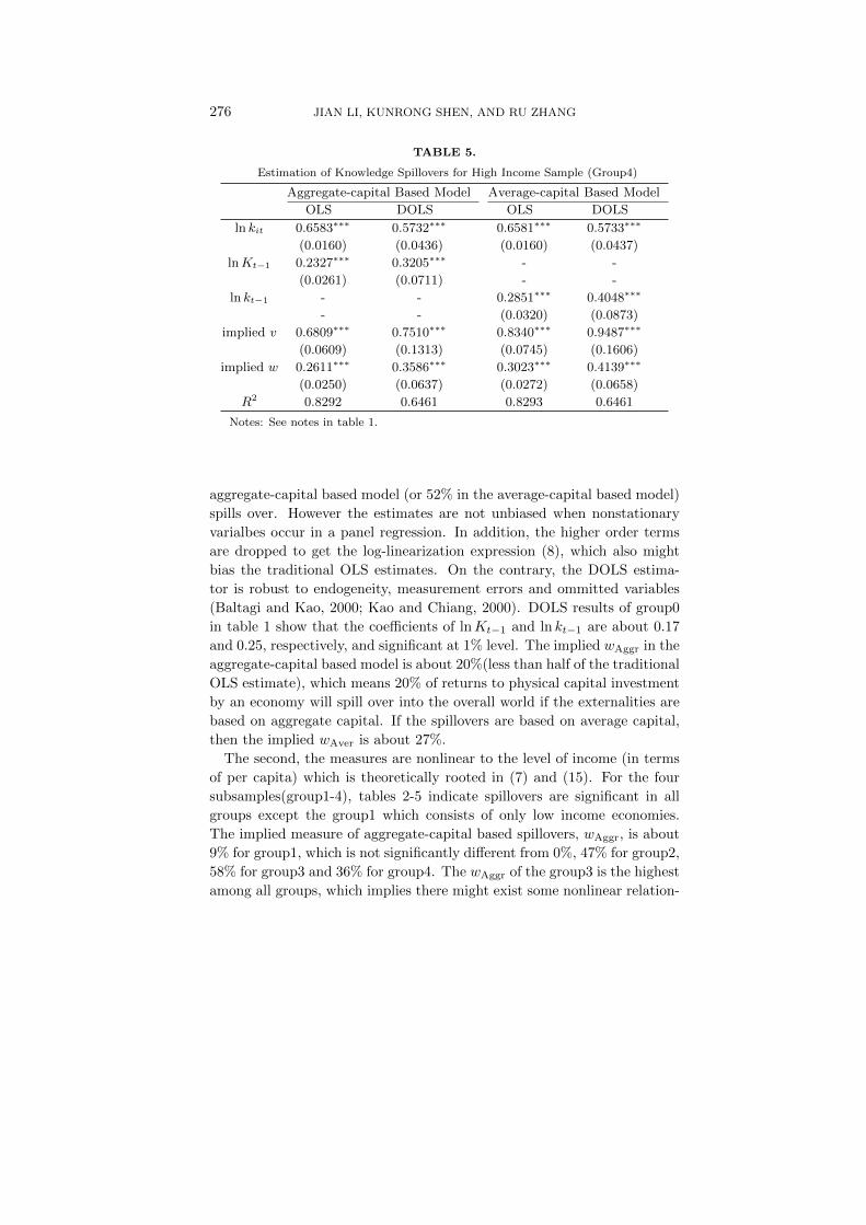
TABLE 5.

Estimation of Knowledge Spillovers for High Income Sample (Group4)


OLS DOLS OLS DOLS

ln kit 0.6583∗∗∗ 0.5732∗∗∗ 0.6581∗∗∗ 0.5733∗∗∗

(0.0160) (0.0436) (0.0160) (0.0437)

lnKt−1 0.2327∗∗∗ 0.3205∗∗∗ - -

(0.0261) (0.0711) - -

ln kt−1 - - 0.2851∗∗∗ 0.4048∗∗∗

- - (0.0320) (0.0873)

implied v 0.6809∗∗∗ 0.7510∗∗∗ 0.8340∗∗∗ 0.9487∗∗∗

(0.0609) (0.1313) (0.0745) (0.1606)

implied w 0.2611∗∗∗ 0.3586∗∗∗ 0.3023∗∗∗ 0.4139∗∗∗

(0.0250) (0.0637) (0.0272) (0.0658)

R2 0.8292 0.6461 0.8293 0.6461


aggregate-capital based model (or 52% in the average-capital based model)

spills over. However the estimates are not unbiased when nonstationary

varialbes occur in a panel regression. In addition, the higher order terms

are dropped to get the log-linearization expression (8), which also might

bias the traditional OLS estimates. On the contrary, the DOLS estima-

tor is robust to endogeneity, measurement errors and ommitted variables

(Baltagi and Kao, 2000; Kao and Chiang, 2000). DOLS results of group0

in table 1 show that the coefficients of lnKt−1 and ln kt−1 are about 0.17

and 0.25, respectively, and significant at 1% level. The implied wAggr in the

aggregate-capital based model is about 20%(less than half of the traditional

OLS estimate), which means 20% of returns to physical capital investment

by an economy will spill over into the overall world if the externalities are

based on aggregate capital. If the spillovers are based on average capital,

then the implied wAver is about 27%.

The second, the measures are nonlinear to the level of income (in terms

of per capita) which is theoretically rooted in (7) and (15). For the four

subsamples(group1-4), tables 2-5 indicate spillovers are significant in all

groups except the group1 which consists of only low income economies.

The implied measure of aggregate-capital based spillovers, wAggr, is about

9% for group1, which is not significantly different from 0%, 47% for group2,

58% for group3 and 36% for group4. The wAggr of the group3 is the highest

among all groups, which implies there might exist some nonlinear relation-


ship between wAggr and the level of income per capita. This conclusion

also applies to wAver.

The third, the elasticity of T to K or k is also estimated and nonlin-

earity of the knowledge function is supported although no specific form of

the knowledge function is assumed. According to tables 1-5, the implied

elasticity of knowledge function is statistically significant at 1% level in

all groups except group1. The implied elasticities are about 0.55, 0.44,

0.74 and 0.75 for group0, group2, group3 and group4, respectively, in the

aggregate-capital based model, and 0.78, 0.52, 1.16 and 0.95 for group0,

group2, group3 and group4, respectively, in the average-capital based mod-

el. Generally it is less than 1 in groups except group3 in the average-capital

model. Just like the measure, it appears that there exists a nonlinear rela-

tionship between the elasticity of knowledge and income level. From table

7, we find the mean of kt monotonically increases with the income level.

Thus it implies that the elasticity of knowledge may not be linear to kt. If

the labor scale is controlled, it will also not be linear to Kt. Unfortunately,

existing literature on knowledge spillovers (e.g., Barro and Sala-I-Martin,

2004; Romer, 1986) unanimously assumes linearity of the knowledge func-

tion, that is, the elasticity of knowledge is 1.

The fourth, it should be noted that, in the group1, the DOLS estimator

in table 2 has an inference different from the traditional OLS estimator.

For a nonstationary panel, the OLS estimates of the coefficients of lnKt−1and ln kt−1 provide spurious results significant at 1% level while the DOLS

estimates suggest no externalities at all. Although it is possible that ex-

ternalities depend on the national income per capita, the more reasonable

explanation would be that capital stock is heterogeneous among countries

with different level of income per capita. For example, the average of

GDP per capita of group1 is about $1379. One will guess that members of

group1 might invest very little on R&D activities which exhibit stronger

externalities than common physical capital.

The fifth, results also suggest that the existence of externalities of phys-

ical capital cannot be excluded only by observing capital’s share in income

(traditionally denoted by α) not substantially different from the elasticity

of y to k. It is true that the elasticity of y to k equals to α in a neoclas-

sical growth model. If evidences support this neoclassical equality, they

will support no externalities, just as argued by Mankiw, Romer, and Weil

(1992). This paper, however, finds that the estimated elasticities of y to k

(the estimated β1 or γ1 in this paper) of group1, group2 and group3 are

very close to 1/3 while positive externalities do exist in group2 and group3


except group1.2 We are not intended to reject the neoclassical model. Our

results just uncover a logical possibility that externalities can exist even if

the elasticity of y to k roughly equals to the capital’s share in income.3

How could it be true? In a global perspective, a country can be con-

sidered as an ”individual” whose capital’s share is just a private share.

By the definition of (9), β1 is corresponding to an individual ’s elasticity

of y to k. In the neoclassical model, β1 equals the capital’s share of that

country. If there are knowledge spillovers, contributions of all inputs in

other countries will benefit from spillovers. Thus the traditional definition

of capital’s share of a country is just the “private” share, not the social

share. Unfortunately previous literature overlooked the difference, such as

Mankiw, Romer, and Weil (1992). Therefore, we can not infer that there

are no externalities of capital stock observing the fact that a private elas-

ticity is equal to a private capital’s share. In this paper, β2 defined by (10)

captures the difference between the “private” and “social” shares of capital

investment. By β1 and β2, the implied social elasticity of y to k is just

β1 + β2.

4. CONCLUSION

In summary, this paper finds a new approach to measure knowledge

spillovers from a perspective of non-appropriable returns to capital stock

without assuming any specific forms of the production and knowledge

functions. The measure of spillovers is defined as the proportion of non-

appropriable returns to social returns, whose theoretical expression is con-

nected with coefficients of familiar regression models. It is very simple

empirically although it appears rather complicated theoretically.

Externalities do exist and cannot be ignored under some circumstances.

The implied measure is about 20% based on aggregate capital (or 27% based

on average capital) in the sample of all economies. There are no significant

externalities for the low income group. But for the other groups, the range

of the measure is 35-58% (or 41-68%) in the aggregate-capital (or average-

capital) based model. The results imply a nonlinear relationship between

the measure and income level.

2Direct measures of the capital’s share in income, α, are roughly 1/3, an empiricaltarget in Mankiw, Romer, and Weil (1992). Moreover, Barro and Sala-I-Martin (2004,table 10.1, pp.439) collects some estimates of α whose range are 0.37-0.42 for OECDcountries, 0.26-0.49 for east Asian countries, and 0.45-0.69 for Latin American countries.

3It is consistent with Howitt (2000) who argues that α < 1 is possible for endogenousgrowth by calibration.


Although we know nothing about the form of the knowledge function,

we can estimate the elasticity of knowledge to its argument. In most cases,

it is less than 1. But for the upper middle income group, it is greater than

1 in the average-capital based model. The elasticity of knowledge function

is also nonlinear to income level.

The paper provides a chance to rethink the traditional opinion about

checking existence of externalities of capital. One cannot argue no exter-

nalities only by means of comparing the elasticity of output to capital with

the direct measure of capital’s share in income of a country. Actually, we

find externalities do or do not exist when the estimated elasticity of output

to capital is roughly close to the direct measure of capital’s share in income.

Future research can be focused on knowledge externalities outside Romer

(1986)’s domain and searching for a unified measure of externalities inde-

pendent on theoretical models. Another interesting issue is to uncover the

nonlinear relationships discussed in the paper. Finally, some important

factors, which might affect the measure of knowledge spillovers, are not

considered in the paper, such as institution environment (Aghion, 2004),

division of labor (Yang and Zhang, 2000) and constitutional transition

(Sachs, Woo, and Yang, 2000).

APPENDIX A

A.1. DATA PREPARATION

The following six aspects describe how the data set is prepared:

1. There are three countries, Nicaragua (group2),Saudi Arabia (group4)

and Sierra Leone (group1), whose investment shares of GDP per capita

are negative in some years (Heston, Summers, and Aten, 2009). But the

corresponding observations are positive in Penn World Table 6.2 (Heston,

Summers, and Aten, 2006), whose base year is 2000. These countries are

excluded because the change of base year should not alter the sign of figures.

2. There are two countries whose average annual growth rates of in-

vestment are negative, that is, Russia(-0.89%, 1990-2007) and Tajikistan(-

4.44%, 1993-2007). The phenomenon might be related to the collapse of

USSR. If the negative gi is used in equation (22), it assumes that the av-

erage growth rate of investment is negative before t = 0. Evidently this is

counterfactual and we exclude Russia and Tajikistan.


3. There are two versions of China’s data. Heston, Summers, and Aten

(2009) thinks the version 2 is more reliable. Thus the version 2 is used in

the paper.

4. We exclude Serbia and Timor-Leste because they have only one ob-

servation in year 2005.

5. Values of real GDP per capita and investment of Bahrain in 2007 are

predicted by means of the average geometric growth rate calculated from

the lastest ten observations available. In 2007, the predicted real GDP per

capita is $27329.847 and the predicted investment is $4125.20 million.

6. Mankiw, Romer, and Weil (1992) suggests that the members of the

Organization of the Petroleum Exporting Countries (OPEC) should be ex-

cluded because their growth facts are more related to natural resources

than to standard inputs. These countries are Angola, Ecuador, Iran, I-

raq, Nigeria, Algeria, Libya, Venezuela, Kuwait, Qatar, Saudi Arabia, and

United Arab Emirates. Indonesia and Gabon were members of OPEC his-

torically and also are excluded. Lesotho and Kiribati are excluded because

a very large fraction of income comes from labor income abroad and has no

relationship with domestic standard inputs, just as Mankiw, Romer, and

Weil (1992) points out.

A.2. ROBUSTNESS

A.2.1. Assumptions of Depreciation Rate

The depreciation rate, δ, is assumed to be 5% in the main part. When

δ deviates from 5%, are our conclusions robust? We list the implied wAggr

and wAver in table 8 when the depreciation rate is assumed to be 0%, 5%,

10%, 15%, 20%, 25%, 30%, and 35%.

Evidently, the nature of conclusions above are not substantially changed.

Positive externalities exist in all groups but the group1. Disturbing δ only

affects the magnitude. When the δ decreases from 35% through 0%, the

range of the implied wAggr is 16%-24%(Group0), 49%-62%(Group2), 60%-

71%(Group3) and 28%-50%(Group4); the range of the implied wAver is

21%-22%(Group0), 54%-67%(Group2), 64%-78%(Group3) and 32%-56%

(Group4). The implied vAggr and vAver are also robust to disturbing δ.

The results are listed in table 9.

A.2.2. Lagged or Current Spillovers

The results above assume lagged spillovers which are reflected by lnKt−1and ln kt−1 in the models (18) and (19). We also consider the current

spillovers which occur in the current year rather than the lagged year.


That is, we estimate the following models for all groups:

ln yit = β0,i + β1 ln kit + β2 lnKt + εit

ln yit = γ0,i + γ1 ln kit + γ2 ln kt + εit

The results are listed in the tables 10 and 11. With δ = 0.05, the results

in the table 10 imply that the measure of knowledge spillovers based on

aggregate capital is about 21%(Group0), 46%(Group2), 59%(Group3) and

36%(Group4); the one based on average capital is about 27%(Group0),

50%(Group2), 69%(Group3) and 41%(Group4). The spillovers for group1

are not significant statistically at 10% level for both types of externalities.

All the conclusions on current spillovers are similar to the ones on lagged

spillovers except for magnitudes. In addition, the conclusions are also ro-

bust to assumptions of rate of depreciation. Conclusions on the elasticity of

knowledge function under current spillovers are similar to the conclusions

under lagged spillovers, as shown in the table 11.

A.2.3. Construction of Initial Capital Stock

The initial capital stock is constructed by (22). Theoretically, the gishould be measured by the growth rate of investment before the time zero

rather than the one after. In the main part of the paper, we use the

average annual growth rate of investment in the sample to meaure gi. If

the economy is on a steady state before and after the year defined to be

zero, the average growth rate before will be equal to the one after since a

steady state is “a situation in which the various quantities grow at constant

rates”. (Barro and Sala-I-Martin, 2004, pp.33) In this circumstance, it is

justified using average annual growth rate of investment in the sample to

calculate the initial capital stock.

If the economy is not on a steady state before time zero while it is after,

there is a problem. Generally the average growth rate is higher when an

economy is not on a steady state than when it is on a steady state. Thus

the initial stock capital is overestimated if average annual growth rate of

investment in the sample is used. How does the overestimation affect the

results? We fabricate a situation to elucidate the effect.

Assume δ = 0.05, I0 = 1, and g = 0.08 (0.08 is the mean growth rate of

investment of all countries in the group0 during the sample period 1950-

2007). Then the initial capital stock is K0 = 7.6923. If the true average

growth rate before the time zero is double, that is, g′ = 0.16, then the

true initial capital stock is K ′0 = 4.7619 = 0.619K0. Suppose the annual


investment is always 1. We calculate capital time series for K0 and K ′0,

respectively.

After 40 years, K40 = 18.3351 and K ′40 = 17.9387. The relative magni-

tude of overestimation is about 2.2%. It implies the overestimation is at-

tenuated greatly. If δ = 0.10 is assumed, K40 = 9.9621 and K ′40 = 9.9140.

Although the relative magnitude of overestimation is 0.5%, the absolute

levels of capital stock are almost half of the ones under the assumption

δ = 0.05.

Therefore the effect of overestimation of initial capital stock is very small

when comparing with the effect of different assumptions of δ. When the

main conclusions of the paper are robust to the assumption of δ, they are

also reasonably considered to be robust to overestimation of initial capital

stock. Therefore the measure of gi in the paper is justified.

A.3. TABLES

TABLE 6.

Definition of Variables

Variable Definition Unit

yit Real GDP per capita of the economy i in the year t USD1

kit Real capital per capita of the economy i in the year t USD1

Kt Real capital of the whole group in the year t USD100,000 million

kt Real capital per capita of the whole group in the year t USD1

Notes: The logarithm of the variable is used in regression models.


TABLE 7.

Summary Statistics

Variable Mean Std. Dev. Min Max

Group0 Total Sample of All Economies

yit 10929.6700 11534.1200 153.4389 77766.1900

kit 33571.8800 40217.5300 29.0177 232014.4000

Kt 1394.7290 214.7331 1070.0850 1767.7040

kt 30543.2700 3266.5240 25553.5300 36161.5100

Group1 Low Income Sample

yit 1378.8990 741.2192 153.4389 3774.3220

kit 1877.8500 1525.2100 213.9011 7750.8280

Kt 13.9271 3.1496 9.8410 20.1640

kt 1855.7960 231.4706 1577.0410 2327.5180

Group2 Lower Middle Income Sample

yit 4442.0550 1978.7500 967.3316 11388.4600

kit 13091.2200 13229.8200 14.0414 70197.5200

Kt 212.9889 60.0819 126.3451 327.3533

kt 9967.6490 2359.5080 6503.1130 14425.7600

Group3 Upper Middle Income Sample

yit 9144.1730 3613.4710 1887.2990 22580.7700

kit 26623.6500 19087.7900 4136.3240 118732.7000

Kt 143.3169 17.8733 115.2701 174.4734

kt 20956.9500 1650.1190 18300.2000 23837.8200

Group4 High Income Sample

yit 25046.8400 10373.2600 1112.7990 77766.1900

kit 80053.1300 38004.1400 390.4237 232014.4000

Kt 957.6996 165.8362 706.3830 1245.7140

kt 97870.1600 13943.1800 76808.9700 122023.3000

Notes: Groups of economies are constructed by the World Bank’s classi-fication. The time range is 1994-2007 for group0 and group3, 1993-2007for group1 and group2, 1990-2007 for group 4. The number of panelunits is 167 for group0, 39 for group1, 43 for group2, 38 for group 3,and 47 for group4. The unit of the variable is described in table 6. Thedepreciation rate of capital stock is assumed to be 5%.


TABLE 8.

The Implied Measure (w) Assuming Lagged Spillovers

δ Group0 Group1 Group2 Group3 Group4

Aggregate-capital Based Model

0% 0.2380 *** 0.2529 0.6193 *** 0.7112 *** 0.4961 ***

(0.0493) (0.2093) (0.0657) (0.1088) (0.0724)

5% 0.2036 *** 0.0894 0.4746 *** 0.5801 *** 0.3586 ***

(0.0403) (0.1501) (0.0509) (0.0876) (0.0637)

10% 0.1907 *** 0.0146 0.4817 *** 0.5906 *** 0.3307 ***

(0.0386) (0.1360) (0.0460) (0.0759) (0.0601)

15% 0.1758 *** −0.0122 0.4895 *** 0.5893 *** 0.3132 ***

(0.0384) (0.1235) (0.0440) (0.0682) (0.0586)

20% 0.1650 *** −0.0164 0.4935 *** 0.5884 *** 0.3005 ***

(0.0383) (0.1125) (0.0430) (0.0622) (0.0584)

25% 0.1588 *** −0.0122 0.4949 *** 0.5899 *** 0.2906 ***

(0.0383) (0.1037) (0.0424) (0.0576) (0.0589)

30% 0.1560 *** −0.0057 0.4948 *** 0.5933 *** 0.2826 ***

(0.0382) (0.0971) (0.0419) (0.0543) (0.0600)

35% 0.1554 *** 0.0001 0.4939 *** 0.5977 *** 0.2757 ***

(0.0380) (0.0924) (0.0416) (0.0518) (0.0614)

Average-capital Based Model

0% 0.2246 *** 0.3446 0.6693 *** 0.7839 *** 0.5645 ***

(0.0717) (0.3005) (0.0624) (0.0896) (0.0681)

5% 0.2650 *** −0.0027 0.5173 *** 0.6841 *** 0.4139 ***

(0.0497) (0.3234) (0.0513) (0.0787) (0.0658)

10% 0.2576 *** −0.0700 0.5248 *** 0.6917 *** 0.3804 ***

(0.0472) (0.2730) (0.0461) (0.0689) (0.0636)

15% 0.2393 *** −0.0648 0.5332 *** 0.6799 *** 0.3601 ***

(0.0472) (0.2244) (0.0439) (0.0642) (0.0630)

20% 0.2243 *** −0.0470 0.5377 *** 0.6660 *** 0.3456 ***

(0.0476) (0.1911) (0.0427) (0.0611) (0.0632)

25% 0.2151 *** −0.0292 0.5396 *** 0.6539 *** 0.3349 ***

(0.0479) (0.1688) (0.0420) (0.0593) (0.0642)

30% 0.2103 *** −0.0143 0.5400 *** 0.6439 *** 0.3263 ***

(0.0479) (0.1536) (0.0415) (0.0587) (0.0656)

35% 0.2085 *** −0.0032 0.5395 *** 0.6352 *** 0.3190 ***

(0.0478) (0.1433) (0.0411) (0.0589) (0.0674)

Notes: *** denotes statistical significance at the 1% level based on the Waldtest. Standard errors are in parentheses. Groups are described in table 7.


TABLE 9.

The Implied Elasticity of Knowledge (v) Assuming Lagged Spillovers



0% 0.5318 *** 0.1212 0.4674 *** 0.6372 *** 0.7474 ***

(0.1023) (0.1026) (0.0707) (0.0876) (0.1029)

5% 0.5516 *** 0.0611 0.4423 *** 0.7418 *** 0.7510 ***

(0.1076) (0.1073) (0.0590) (0.1176) (0.1313)

10% 0.5180 *** 0.0110 0.4716 *** 0.7807 *** 0.7562 ***

(0.1073) (0.1040) (0.0579) (0.1181) (0.1414)

15% 0.4691 *** −0.0100 0.4861 *** 0.7644 *** 0.7269 ***

(0.1059) (0.1004) (0.0573) (0.1103) (0.1436)

20% 0.4331 *** −0.0144 0.4906 *** 0.7454 *** 0.6955 ***

(0.1046) (0.0973) (0.0566) (0.1020) (0.1448)

25% 0.4123 *** −0.0112 0.4898 *** 0.7357 *** 0.6689 ***

(0.1036) (0.0945) (0.0558) (0.0961) (0.1471)

30% 0.4026 *** −0.0054 0.4865 *** 0.7346 *** 0.6470 ***

(0.1029) (0.0920) (0.0550) (0.0926) (0.1504)

35% 0.3995 *** 0.0001 0.4820 *** 0.7392 *** 0.6285 ***

(0.1025) (0.0899) (0.0543) (0.0908) (0.1543)


0% 0.4931 *** 0.1883 0.5817 *** 0.9387 *** 0.9846 ***

(0.1617) (0.2028) (0.0907) (0.1284) (0.1238)

5% 0.7778 *** −0.0017 0.5247 *** 1.1634 *** 0.9487 ***

(0.1564) (0.2005) (0.0708) (0.1887) (0.1606)

10% 0.7626 *** −0.0489 0.5604 *** 1.2156 *** 0.9402 ***

(0.1554) (0.1809) (0.0691) (0.1937) (0.1743)

15% 0.6917 *** −0.0504 0.5790 *** 1.1334 *** 0.8971 ***

(0.1527) (0.1666) (0.0682) (0.1779) (0.1775)

20% 0.6340 *** −0.0399 0.5857 *** 1.0420 *** 0.8556 ***

(0.1504) (0.1568) (0.0672) (0.1613) (0.1793)

25% 0.5986 *** −0.0264 0.5860 *** 0.9693 *** 0.8224 ***

(0.1488) (0.1492) (0.0662) (0.1500) (0.1825)

30% 0.5799 *** −0.0134 0.5832 *** 0.9138 *** 0.7958 ***

(0.1477) (0.1433) (0.0651) (0.1436) (0.1869)

35% 0.5718 *** −0.0031 0.5787 *** 0.8698 *** 0.7738 ***

(0.1468) (0.1387) (0.0642) (0.1405) (0.1919)



TABLE 10.

The Implied Measure (w) Assuming Current Spillovers



0% 0.2237 *** 0.2073 0.6314 *** 0.7326 *** 0.4879 ***

(0.0469) (0.2211) (0.0619) (0.0908) (0.0724)

5% 0.2060 *** 0.0965 0.4600 *** 0.5892 *** 0.3580 ***

(0.0384) (0.1433) (0.0508) (0.0789) (0.0631)

10% 0.2030 *** 0.0477 0.4587 *** 0.5973 *** 0.3326 ***

(0.0367) (0.1239) (0.0468) (0.0694) (0.0592)

15% 0.1917 *** 0.0304 0.4641 *** 0.5987 *** 0.3175 ***

(0.0364) (0.1111) (0.0448) (0.0624) (0.0574)

20% 0.1795 *** 0.0217 0.4682 *** 0.6003 *** 0.3068 ***

(0.0366) (0.1023) (0.0437) (0.0566) (0.0567)

25% 0.1694 *** 0.0172 0.4708 *** 0.6032 *** 0.2984 ***

(0.0368) (0.0958) (0.0430) (0.0522) (0.0568)

30% 0.1615 *** 0.016 0.4722 *** 0.6069 *** 0.2915 ***

(0.0369) (0.0909) (0.0424) (0.0489) (0.0574)

35% 0.1556 *** 0.0161 0.4728 *** 0.6105 *** 0.2855 ***

(0.0371) (0.0872) (0.0420) (0.0465) (0.0583)


0% 0.2133 *** 0.0119 0.6855 *** 0.7914 *** 0.5387 ***

(0.0683) (0.5641) (0.0571) (0.0778) (0.0718)

5% 0.2670 *** −0.3362 0.5033 *** 0.6896 *** 0.4058 ***

(0.0472) (0.5232) (0.0513) (0.0705) (0.0663)

10% 0.2707 *** −0.1672 0.5016 *** 0.7021 *** 0.3774 ***

(0.0443) (0.3034) (0.0471) (0.0605) (0.0634)

15% 0.2579 *** −0.0585 0.5072 *** 0.7004 *** 0.3606 ***

(0.0441) (0.2103) (0.0450) (0.0544) (0.0621)

20% 0.2430 *** −0.0165 0.5117 *** 0.6978 *** 0.3489 ***

(0.0446) (0.1723) (0.0438) (0.0496) (0.0618)

25% 0.2303 *** 0.0006 0.5147 *** 0.6971 *** 0.3401 ***

(0.0451) (0.1526) (0.0429) (0.0458) (0.0622)

30% 0.2204 *** 0.0097 0.5165 *** 0.6975 *** 0.3330 ***

(0.0455) (0.1404) (0.0422) (0.0431) (0.0630)

35% 0.2128 *** 0.0152 0.5175 *** 0.6979 *** 0.3269 ***

(0.0458) (0.1322) (0.0417) (0.0412) (0.0642)



TABLE 11.

The Implied Elasticity of Knowledge (v) Assuming Current Spillovers



0% 0.4907 *** 0.0892 0.4747 *** 0.7280 *** 0.7494 ***

(0.1034) (0.0983) (0.0697) (0.0791) (0.1031)

5% 0.5629 *** 0.0649 0.4206 *** 0.7820 *** 0.7550 ***

(0.1091) (0.1013) (0.0593) (0.1095) (0.1300)

10% 0.5614 *** 0.0367 0.4339 *** 0.8110 *** 0.7660 ***

(0.1084) (0.0980) (0.0576) (0.1103) (0.1399)

15% 0.5210 *** 0.0255 0.4424 *** 0.8007 *** 0.7438 ***

(0.1065) (0.0948) (0.0564) (0.1032) (0.1420)

20% 0.4778 *** 0.0192 0.4466 *** 0.7887 *** 0.7174 ***

(0.1046) (0.0920) (0.0553) (0.0953) (0.1427)

25% 0.4430 *** 0.0159 0.4482 *** 0.7831 *** 0.6940 ***

(0.1030) (0.0895) (0.0544) (0.0892) (0.1441)

30% 0.4170 *** 0.0152 0.4482 *** 0.7823 *** 0.6740 ***

(0.1019) (0.0872) (0.0535) (0.0848) (0.1462)

35% 0.3977 *** 0.0156 0.4471 *** 0.7841 *** 0.6570 ***

(0.1011) (0.0853) (0.0527) (0.0816) (0.1489)


0% 0.4617 *** 0.0041 0.6042 *** 1.0080 *** 0.9186 ***

(0.1593) (0.1962) (0.0887) (0.1174) (0.1256)

5% 0.7901 *** −0.1530 0.5002 *** 1.2112 *** 0.9248 ***

(0.1579) (0.1891) (0.0708) (0.1732) (0.1592)

10% 0.8180 *** −0.1048 0.5154 *** 1.2895 *** 0.9319 ***

(0.1563) (0.1682) (0.0685) (0.1758) (0.1725)

15% 0.7636 *** −0.0448 0.5259 *** 1.2560 *** 0.9016 ***

(0.1527) (0.1544) (0.0668) (0.1607) (0.1755)

20% 0.7010 *** −0.0141 0.5317 *** 1.2150 *** 0.8688 ***

(0.1494) (0.1455) (0.0654) (0.1450) (0.1767)

25% 0.6501 *** 0.0005 0.5344 *** 1.1882 *** 0.8410 ***

(0.1468) (0.1388) (0.0641) (0.1331) (0.1787)

30% 0.6120 *** 0.0091 0.5352 *** 1.1719 *** 0.8180 ***

(0.1448) (0.1336) (0.0630) (0.1249) (0.1816)

35% 0.5836 *** 0.0147 0.5346 *** 1.1599 *** 0.7986 ***

(0.1433) (0.1294) (0.0620) (0.1191) (0.1851)



TABLE 12.

Unit Root Tests for Total Sample (Group0)

Option Test ln yit ln kit Test lnKt ln kt

c LLC(2002), Adj-t∗ 1.6743 −0.6562 ADF −0.5158 −0.2018

c,t −19.0485∗∗∗ −7.5057∗∗∗ −3.1571∗ −3.2393∗

c HT(1999), z 8.6367 5.0007 PP −0.7973 0.3461

c,t 6.0880 3.0755 −1.4115 −1.6134

c Breitung(2000), λ∗ 4.6288 0.9529

c,t 1.9154 −1.1408

c IPS(2003), t-bar −0.4028 −0.6618

c,t −1.9287 −1.4805

c Hadri(2000), z 83.9098*** 89.0050 ***

c,t 46.0396*** 50.6282 ***

Notes: ***, significant at 1% level; **, significant at 5% level; *, significant at 10% level. Lags are 3years in Breitung(2000), ADF and PP. Lags in LLC(2002) are automatically selected according toAkaike information criterion(AIC) with the maximum of 3 years. There are no lags in HT(1999),IPS(2003) and Hadri(2000). ADF and PP are Augmented Dickey-Fuller and Phillips-Perron unit-root tests, respectively. The option, c, denotes inclusion of a constant term. The option, t, denotesinclusion of a trend term.

TABLE 13.

Unit Root Tests for Low Income Sample (Group1)


c LLC(2002), Adj-t∗ 1.2373 −2.9472∗∗∗ ADF 1.0905 2.1287

c,t −3.8337∗∗∗ −8.9121∗∗∗ −1.5304 1.1728

c HT(1999), z 2.5048 4.3518 PP 10.7360 9.4658

c,t 0.7966 7.5340 −0.0097 −0.2872

c Breitung(2000), λ∗ 1.1349 −1.2991∗

c,t 0.7719 0.5491

c IPS(2003), t-bar −0.9795 −0.8710

c,t −2.8470∗∗∗ −1.6364

c Hadri(2000), z 36.7196 *** 47.0368 ***

c,t 23.6837 *** 33.6948 ***



TABLE 14.

Unit Root Tests for Lower Middle Income Sample (Group2)


c LLC(2002), Adj-t∗ 5.4076 0.5655 ADF 0.4920 0.8420

c,t −7.0114∗∗∗ −8.9659∗∗∗ −3.7201∗∗ −2.7055

c HT(1999), z 6.5047 0.3413 PP −0.5591 −0.1447

c,t 1.4438 3.9227 −1.8941 −1.7407

c Breitung(2000), λ∗ 3.5692 2.1976

c,t 1.9844 −0.1267

c IPS(2003), t-bar −0.3579 −0.8911

c,t −2.0574 −1.8158

c Hadri(2000), z 45.7609 *** 44.3176 ***

c,t 23.1138 *** 29.9836 ***


TABLE 15.

Unit Root Tests for Upper Middle Income Sample (Group3)


c LLC(2002), Adj-t∗ 8.5652 −2.6027∗∗∗ ADF −0.4325 −0.3478

c,t −6.4583∗∗∗ −6.3140∗∗∗ −4.3645∗∗∗ −4.1582∗∗∗

c HT(1999), z 4.6935 5.2259 PP −0.4947 −0.1944

c,t 2.5721 8.2510 −1.5646 −1.5666

c Breitung(2000), λ∗ 3.1853 1.0690

c,t 1.8426 −1.0494

c IPS(2003), t-bar 0.0457 −1.1113

c,t −1.7033 −1.0845

c Hadri(2000), z 37.4999 *** 45.5424 ***

c,t 19.4776 *** 29.6981 ***

Notes: See footnotes in table 12.


TABLE 16.

Unit Root Tests for High Income Sample (Group4)


c LLC(2002), Adj-t∗ 1.7281 4.6392 ADF −1.0600 −0.3243

c,t −8.4982∗∗∗ −10.5151∗∗∗ −1.4386 −3.1474∗

c HT(1999), z 6.5973 6.2711 PP −1.2809 −0.2095

c,t 1.3305 7.8798 −1.4450 −1.6798

c Breitung(2000), λ∗ 4.8279 0.6943

c,t 1.1477 0.4223

c IPS(2003), t-bar 0.1488 0.5523

c,t −2.8184∗∗∗ −0.6430

c Hadri(2000), z 66.7367 *** 70.0638 ***

c,t 21.8999 *** 32.9676 ***

Notes: See footnotes in table 12.

TABLE 17.

Cointegration Tests for Total Sample (Group0)

Statistic Aggregate-capital Average-capital

Based Model Based Model

Panel v-statistic 12.9849 *** 12.9722 ***

Panel rho-statistic −42.8057∗∗∗ −42.4781∗∗∗

Panel t-statistic(Nonparametric) −17.4309∗∗∗ −17.3059∗∗∗

Panel t-statistic(Parametric) −586.9367∗∗∗ −578.6917∗∗∗

Group rho-statistic −51.7832∗∗∗ −51.6988∗∗∗

Group t-statistic(Nonparametric) −19.2158∗∗∗ −19.1658∗∗∗

Group t-statistic(Parametric) −20.6868∗∗∗ −20.6529∗∗∗

Notes: ***, significant at 1% level. Tests are based on Pedroni (1999) andtaken with a constant option.

TABLE 18.

Cointegration Tests for Low Income Sample (Group1)












TABLE 19.

Cointegration Tests for Lower Middle Income Sample (Group2)











TABLE 20.

Cointegration Tests for Upper Middle Income Sample (Group3)











TABLE 21.

Cointegration Tests for High Income Sample (Group4)












REFERENCES

Aghion, Philippe, 2004. Growth and Development: A Schumpeterian Approach. An-nals of Economics and Finance 5(1), 1-25.

Arrow, Kenneth, J., 1962. The Economic Implications of Learning by Doing. TheReview of Economic Studies 29(3), 155–173.

Baltagi, Badi, H. and Chihwa Kao, 2000. Nonstationary Panels, Cointegration inPanels and Dynamic Panels: A Survey. In Nonstationary Panels, Panel Cointegration,and Dynamic Panels, Advances in Econometrics, vol. 15, edited by Badi H. Baltagi,Thomas B. Fomby, and R. Carter Hill. Elsevier Science Inc, 7–51.

Barro, Robert, J. and Xavier Sala-I-Martin, 2004. Economic Growth. Cambridge,Massachusetts: Massachusetts Institute of Technology, 2nd ed.

Breitung, Jorg, 2000. The Local Power of Some Unit Root Tests for Panel Data.In Nonstationary Panels, Panel Cointegration, and Dynamic Panels, Advances inEconometrics, vol. 15, edited by Badi H. Baltagi, Thomas B. Fomby, and R. CarterHill. Elsevier Science Inc, 161–177.

Bresnahan, Timothy, F., 1986. Measuring the Spillovers from Technical Advance:Mainframe Computers in Financial Services. The American Economic Review 76(4),742–755.

Chiang, Min-Hsien and Chihwa Kao, 2002. Nonstationary Panel Time Series UsingNPT 1.3 - A User Guide. Center for Policy Research, Syracuse University.

Coe, David, T. and Elhanan Helpman, 1995. International R&D Spillovers. EuropeanEconomic Review 39(5), 859-887.

Coe, David, T., Elhanan Helpman, and Alexander, W. Hoffmaister, 2009. Interna-tional R&D Spillovers and Institutions. European Economic Review 53(7), 723–741.

Griliches, Zvi, 1992. The Search for R&D Spillovers. The Scandinavian Journal ofEconomics 94, S29-S47.

Grossman, Gene, M. and Elhanan Helpman, 1991. Innovation and Growth in theGlobal Economy. Cambridge: MIT Press.

Hadri, Kaddour, 2000. Testing for Stationarity in Heterogeneous Panel Data. TheEconometrics Journal 3(2), 148–161.

Harris, Richard D. F. and Elias Tzavalis, 1999. Inference for Unit Roots in DynamicPanels Where the Time Dimension is Fixed. Journal of Econometrics 91(2), 201–226.

Heston, Alan, Robert Summers, and Bettina Aten, 2006. Penn World Table Version6.2. Tech. rep., Center for International Comparisons of Production, Income andPrices at the University of Pennsylvania.

Heston, Alan, Robert Summers, and Bettina Aten, 2009. Penn World Table Version6.3. Tech. rep., Center for International Comparisons of Production, Income andPrices at the University of Pennsylvania.

Howitt, Peter, 2000. Endogenous Growth and Cross-Country Income Differences. TheAmerican Economic Review 90(4), 829-846.

Im, Kyung, So, M. Hashem Pesaran, and Yongcheol Shin, 2003. Testing for UnitRoots in Heterogeneous Panels. Journal of Econometrics 115(1), 53–74.

Jones, Charles, I. and John, C. Williams, 1998. Measuring the Social Return to R&D.The Quarterly Journal of Economics 113(4), 1119–1135.

Kaiser, Ulrich, 2002. Measuring Knowledge Spillovers in Manufacturing and Services:An Empirical Assessment of Alternative Approaches. Research Policy 31(1), 125–144.


Kao, Chihwa and Min-Hsien Chiang, 2000. On the Estimation and Inference of aCointegrated Regression in Panel Data. In Nonstationary Panels, Panel Cointegra-tion, and Dynamic Panels, Advances in Econometrics, vol. 15, edited by Badi H.Baltagi, Thomas B. Fomby, and R. Carter Hill. Elsevier Science Inc., 179–222.

Lang, Guenter, 2009. Measuring the Returns of R&D–An Empirical Study of theGerman Manufacturing Sector over 45 Years. Research Policy 38(9), 1438–1445.

Levin, Andrew, Chien-Fu Lin, and Chia-Shang James Chu, 2002. Unit Root Testsin Panel Data: Asymptotic and Finite-Sample Properties. Journal of Econometrics108(1), 1–24.

Mankiw, N. Gregory, David Romer, and David N. Weil, 1992. A Contribution tothe Empirics of Economic Growth. The Quarterly Journal of Economics 107(2),407–437.

Mansfield, Edwin, John Rapoport, Anthony Romeo, Samuel Wagner, and GeorgeBeardsley, 1977. Social and Private Rates of Return from Industrial Innovations. TheQuarterly Journal of Economics 91(2), 221–240.

Nelson, Andrew J. 2009. Measuring Knowledge Spillovers: What Patents, Licensesand Publications Reveal About Innovation Diffusion. Research Policy 38(6), 994–1005.

Pedroni, Peter, 1999. Critical Values for Cointegration Tests in Heterogeneous Panelswith Multiple Regressors. Oxford Bulletin of Economics and Statistics 61(S1), 653–670.

Romer, Paul M. 1986. Increasing Returns and Long-Run Growth. The Journal ofPolitical Economy 94(5), 1002–1037.

Sachs, Jeffrey, Wing Thye Woo, and Xiaokai Yang, 2000. Economic Reforms andConstitutional Transition. Annals of Economics and Finance 1(2), 423-479.

Shen, Kunrong and Jian Li. 2009. Measurement of Technology Spillovers. EconomicResearch Journal 4, 77–89.

Trajtenberg, Manuel, 1989. The Welfare Analysis of Product Innovations, with anApplication to Computed Tomography Scanners. The Journal of Political Economy97(2), 444–479.

Yang, Xiaokai and Dingsheng Zhang, 2000. Endogenous Structure of the Division ofLabor, Endogenous Trade Policy Regime, and a Dual Structure in Economic Devel-opment. Annals of Economics and Finance 1(1), 211-230.

measuring knowledge spillovers: a non-appropriable …down.aefweb.net/aefarticles/aef120204.pdf ·...

Documents