TKK Dissertations 7Espoo 2005

MEASURING OF NOISE AND WEARING OF QUIETSURFACESDoctoral Dissertation

Helsinki University of TechnologyDepartment of Civil and Environmental EngineeringLaboratory of Highway Engineering

Nina Raitanen

TKK Dissertations 7Espoo 2005

MEASURING OF NOISE AND WEARING OF QUIETSURFACESDoctoral Dissertation

Nina Raitanen

Dissertation for the degree of Doctor of Science in Technology to be presented with due permission of the Department of Civil and Environmental Engineering for public examination and debate in Auditorium R1 at Helsinki University of Technology (Espoo, Finland) on the 9th of June, 2005, at 12 noon.

Helsinki University of TechnologyDepartment of Civil and Environmental EngineeringLaboratory of Highway Engineering

Teknillinen korkeakouluRakennus- ja ympäristötekniikan osastoTietekniikan laboratorio

Distribution:Helsinki University of TechnologyDepartment of Civil and Environmental EngineeringLaboratory of Highway EngineeringP.O.Box 2100FI - 02015 TKKFINLANDTel. +358-9-4511fax +358-9-451 5019URL: http://www.tkk.fi/Units/Civil/Highway/E-mail: nina.raitanen@tieliikelaitos.fi

© 2005 Nina Raitanen

ISBN 951-22-7693-3ISBN 951-22-7694-1 (PDF)ISSN 1795-2239ISSN 1795-4584 (PDF) URL: http://lib.tkk.fi/Diss/2005/isbn9512276941/

TKK-DISS-2005

Otamedia OyEspoo 2005

3

HELSINKI UNIVERSITY OF TECHNOLOGY P.O.BOX 1000, FI- 02015 HUT http://www.hut.fi/

ABSTRACT OF DOCTORAL DISSERTATION

Author Raitanen Nina Name of the dissertation MEASURING OF NOISE AND WEARING OF QUIET SURFACES Date of manuscript 23 August, 2004 Date of dissertation 9 June, 2005 X Monograph □Article dissertation (summary +original articles)) Department Civil and Environmental Engineering

Laboratory Highway Engineering

Field of research Asphalt surfaces

Opponent(s) Managing Director, Dr Heikki Jämsä, Finnish Asphalt Association

Researcher, Dr Roger Nilsson, Skanska Ab

Supervisor Professor Esko Ehrola (HUT)

(Instructor)

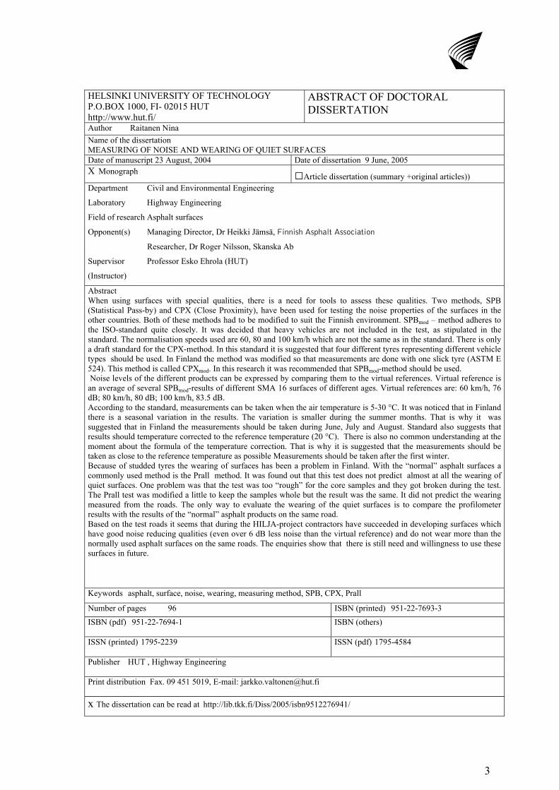
Abstract When using surfaces with special qualities, there is a need for tools to assess these qualities. Two methods, SPB (Statistical Pass-by) and CPX (Close Proximity), have been used for testing the noise properties of the surfaces in the other countries. Both of these methods had to be modified to suit the Finnish environment. SPBmod – method adheres to the ISO-standard quite closely. It was decided that heavy vehicles are not included in the test, as stipulated in the standard. The normalisation speeds used are 60, 80 and 100 km/h which are not the same as in the standard. There is only a draft standard for the CPX-method. In this standard it is suggested that four different tyres representing different vehicle types should be used. In Finland the method was modified so that measurements are done with one slick tyre (ASTM E 524). This method is called CPXmod. In this research it was recommended that SPBmod-method should be used. Noise levels of the different products can be expressed by comparing them to the virtual references. Virtual reference is an average of several SPBmod-results of different SMA 16 surfaces of different ages. Virtual references are: 60 km/h, 76 dB; 80 km/h, 80 dB; 100 km/h, 83.5 dB. According to the standard, measurements can be taken when the air temperature is 5-30 °C. It was noticed that in Finland there is a seasonal variation in the results. The variation is smaller during the summer months. That is why it was suggested that in Finland the measurements should be taken during June, July and August. Standard also suggests that results should temperature corrected to the reference temperature (20 °C). There is also no common understanding at the moment about the formula of the temperature correction. That is why it is suggested that the measurements should be taken as close to the reference temperature as possible Measurements should be taken after the first winter. Because of studded tyres the wearing of surfaces has been a problem in Finland. With the “normal” asphalt surfaces a commonly used method is the Prall method. It was found out that this test does not predict almost at all the wearing of quiet surfaces. One problem was that the test was too “rough” for the core samples and they got broken during the test. The Prall test was modified a little to keep the samples whole but the result was the same. It did not predict the wearing measured from the roads. The only way to evaluate the wearing of the quiet surfaces is to compare the profilometer results with the results of the “normal” asphalt products on the same road. Based on the test roads it seems that during the HILJA-project contractors have succeeded in developing surfaces which have good noise reducing qualities (even over 6 dB less noise than the virtual reference) and do not wear more than the normally used asphalt surfaces on the same roads. The enquiries show that there is still need and willingness to use these surfaces in future.

Keywords asphalt, surface, noise, wearing, measuring method, SPB, CPX, Prall

Number of pages 96 ISBN (printed) 951-22-7693-3

ISBN (pdf) 951-22-7694-1

ISBN (others)

ISSN (printed) 1795-2239

ISSN (pdf) 1795-4584

Publisher HUT , Highway Engineering Print distribution Fax. 09 451 5019, E-mail: jarkko.valtonen@hut.fi x The dissertation can be read at http://lib.tkk.fi/Diss/2005/isbn9512276941/

4

TEKNILLINEN KORKEAKOULU PL 1000, 02015 TKK http://www.hut.fi/

VÄITÖSKIRJAN TIIVISTELMÄ

Tekijä Raitanen Nina Väitöskirjan nimi MEASURING OF NOISE AND WEARING OF QUIET SURFACES Käsikirjoituksen jättämispäivämäärä 23.8.2005 Väitöstilaisuuden ajankohta 9.6.2005 X Monografia □Yhdistelmäväitöskirja (yhteenveto+erillisartikkelit) Osasto Rakennus- ja ympäristötekniikan osasto

Laboratorio Tietekniikka

Tutkimusala Päällystetekniikka

Vastaväittäjä(t) Toimitusjohtaja, tekn. tri. Heikki Jämsä Asfalttiliitto ry

Tutkija, tekn.tri Roger Nilsson, Skanska Ab

Työn valvoja Professori Esko Ehrola (TKK)

Työn ohjaaja

Tiivistelmä Arvioitaessa päällysteitä, joilla on toiminnallisia ominaisuuksia, tarvitaan työkaluja näiden ominaisuuksien arvioimiseksi. Useissa maissa on kahta eri mittausmenetelmää käytetty päällysteiden meluominaisuuksien arviointiin. Käytetyt menetelmät ovat: SPB (Statistical Pass-by) ja CPX (Close Proximity). Tässä tutkimuksessa molempia mittausmenetelmiä modifioitiin Suomen oloihin sopiviksi. SPBmod – menetelmä noudattaa melko tarkastit menetelmän ISO-standardia. Standardista poiketaan siinä, että raskaita ajoneuvoja ei sisällytetty mittauksiin. Lisäksi käytettävät tulosten normalisointinopeudet ovat poikkeavasti 60, 80 and 100 km/h. CPX-metodista on toistaiseksi olemassa vain standardiluonnos. Luonnoksen mukaan mittauksissa tulisi käyttää neljää mittarengasta, jotka edustavat eri ajoneuvotyyppejä. Suomessa mittaukset tehtiin yhdellä sileällä renkaalla (ASTM E 524). Tätä mittaustapaa kutsutaan nimellä CPXmod. Tutkimuksessa päädytään suosittelemaan SPBmod-menetelmän käyttöä. Hiljaisen päällysteen meluominaisuuksia voidaan arvioida vertaamalla niitä referenssipäällysteeseen. Referenssipäällyste on virtuaalinen SMA 16 päällyste eli keskiarvo useasta SPBmod-mittauksesta eri ikäisillä SMA 16 päällysteillä. Virtuaalisten referenssipäällysteiden mittaustulokset ovat seuraavat: 60 km/h , 76 dB; 80 km/h, 80 dB; 100 km/h, 83.5 dB. Standardien mukaan melumittauksia voidaan tehdä ilman lämpötilan ollessa 5-30 °C. Suomessa havaittiin kuitenkin, että tuloksissa esiintyi kausittaista vaihtelua. Vaihtelu oli pienintä kesäkuukausien aikana. Tämän vuoksi päädytään suosittelemaan, että Suomessa melumittaukset tulisi tehdä kesä-, heinä-tai elokuussa. Standardissa suositellaan myös, että melumittaustulokset tulisi lämpötilakorjata referenssilämpötilaan (20 °C) mutta lämpötilakorjauksen kaavasta ei ole yksimielisyyttä. Suositeltavaa onkin, että mittaukset tehdään mahdollisimman lähellä referenssilämpötilaa. Päällysteen meluominaisuudet tulee arvioida aikaisintaan yhden talven käytön jälkeen. Nastarenkaiden käytön vuoksi päällysteiden urautuminen on Suomessa ongelma. Tavallisten päällysteiden urautumista voidaan ennustaa Prall-kokeella. Menetelmää kokeiltiin myös hiljaisille päällysteille mutta se ei ennustanut näiden urautumista juuri lainkaan. Kokeen tekemisessä ongelmaksi osoittautui se, että koekappaleet hajosivat. Prall-kokeen asetuksia muokattiin, jolloin kappaleet saatiin pysymään koossa. Myöskään tämä modifioitu Prall-menetelmä ei ennustanut hiljaisten päällysteiden todellista kulumista. Tällä hetkellä hiljaisten päällysteiden kulumisominaisuuksia voidaan arvioida ainoastaan vertaamalla niiden ja ”tavallisten” asfalttipäällysteiden laserprofilometrillä mitattua urautumista samalla tiellä. Koeteiltä mitattujen tulosten perusteella voidaan päätellä, että urakoitsijat ovat onnistuneet HILJA-projektin aikana kehittämään päällysteitä, jotka ovat melua vähentäviä (jopa 6 dB virtuaaliseen referenssiin verrattuna) ja jotka eivät kulu enempää kuin tavallisesti käytetyt päällystetyypit samoilla teillä. Kyselyt osoittivat, että hiljaisille päällysteille on edelleen kysyntää.

Avainsanat asfaltti, päällyste, melu, urautuminen, mittausmenetelmä, SPB, CPX, Prall

Sivumäärä 96 ISBN (painettu) 951-22-7693-3 ISBN (pdf) 951-22-7694-1

ISBN (muut)

ISSN (painettu) 1795-2239

ISSN (pdf) 1795-4584

Julkaisija TKK , tietekniikan laboratorio Painetun väitöskirjan jakelu Fax. 09 451 5019, E-mail: jarkko.valtonen@hut.fi

X Luettavissa verkossa osoitteessa http://lib.tkk.fi/Diss/2005/isbn9512276941/

5

ACKNOWLEDGEMENTS It is obvious that this research would not have been possible without the HILJA-research. I want to thank all the participants of that project for allowing me to use these results for my own purposes as well. Different scholarships have kept me alive during these years. The Research Foundation of the HUT, Technological Foundation and The Finnish Cultural Foundation have all given their financial support for this research. My professor, Dr Esko Ehrola, thank you for seeing this whole process through and, in the same sentence, I want to thank my ex-boss, Mr Juhani Tervala at the Ministry of Transport and Communication, for allowing me to leave my work for these years (and for giving me extra years when I asked). This work would have been hard without my colleagues in the HUT, Laboratory of Highway engineering. I can honestly say that without you, Ilmo and Marko, I would not have been able to do this work. Thank you Petri for doing all the laboratory work for me and for being always ready for my new ideas. Those summers along the roadside would not have been the same without you Katja. Thank you Ute, Kari, Marja and Ville for giving me your support, especially with the computers and you Pekka for singing together in our room. You have been here most of the time I have been working and all those others who came and left during this process, you have been an essential part of the good spirit in the Laboratory. Last but not least, warm thanks to you Jarkko, for believing in me even though it must have been sometimes difficult. Special thanks to Mr Panu Sainio for being always available. My motto with difficult questions has been: Let’s ask Panu; if he doesn’t know the answer, no one does. The whole crew of the Automotive Engineering has been unbelievably nice and supporting. Thank you for giving me all the support with those difficult technical devices (and for giving me new ones when I broke them). The whole home crew, Pasi and all those four legged, hairy creatures, as well as my friends, you deserve special thanks for living together with me through this interesting period of my life. I want to dedicate this book for my Mummi who never saw this completed but who always was so proud of her granddaughter’s studies. It is important for me that you, Pappa, are still here to see this happen.

6

DEFINITIONS AC Asphalt Concrete ADT Average Daily Traffic ASTO Asfalttipäällysteiden tutkimusohjelma

(Recearch program of asphalt surfaces) CB Coast-by-method CPX Close Proximity-method CPXmod Modified Close Proximity-method CPXI Close Proximity Sound Index CRTN Calculation of Road Traffic Noise (name of the report) dB decibel value (in this research used also from the A-weighted dB) dB(A) A-weighted decibel value (unofficial symbol but commonly used) FinnRA Finnish Road Administration HAPAS Highway Authorities Product Approval Scheme HILJA Hiljaisten päällysteiden tutkimusprojekti

(Research program of quiet surfaces) HRA Hot Rolled Asphalt HUT Helsinki University of Technology ICT Intensive Compaction Tester INSIDE Noise measurements inside the vehicle ISO International Organisation for Standardisation LAeq A-weighted, equivalent sound pressure level LAmax A-weighted, maximum sound pressure level Lden indicator of the overall noise level during the day, evening and night Lnight indicator for the sound level during the night Lp Sound pressure level LAE noise exposure level MOBILE Liikenteen energian käytön ja ympäristövaikutusten tutkimusohjelma

(Research program: Developing solutions for the Environmental Issues in Transportation)

NOTRA Noise Trailer OA Open asphalt PA Porous Asfalt PANK Finnish Pavement Technology Advisory Council PWR Pavement Wearing Ratio rpm rotation per minute rutting deformation + wearing of the surface SMA Stone Mastic Asphalt SPB Statistical Pass-by-method SPB mod Modified Statistical Pass-by-method SPB mod (cal) Statistical Pass-by-result calculated from the CPXmod-results SPBI Statistical Pass-by Index TEKES National Technology Agency of Finland TINO EU-project (Tyre Noise, Brite Euram, BRPR 950121) tyre/road interaction between the tyre and the road surface U.K. United Kingdom VTT Technical Research Centre of Finland

7

TABLE OF CONTENTS ABSTRACT OF DOCTORAL DISSERTATION ..……………………………………………………..3

VÄITÖSKIRJAN TIIVISTELMÄ ……………………………………………………………………….4

ACKNOWLEDGEMENTS ....................................................................................................................... 5

DEFINITIONS ........................................................................................................................................... 6

TABLE OF CONTENTS............................................................................................................................ 7

1 BACKGROUND AND THE AIM OF THE RESEARCH............................................................. 9

2 SOUND AND NOISE ...................................................................................................................... 11 2.1 BASIC DEFINITIONS OF SOUND AND NOISE......................................................... 11

2.1.1 Sound pressure level ................................................................................ 11 2.1.2 Sound propagation and suppression ....................................................... 12 2.1.3 Frequency and A-weighting..................................................................... 15 2.1.4 Doppler effect .......................................................................................... 15 2.1.5 Maximum and equivalent sound pressure levels ..................................... 16

2.2 NOISE PROBLEM................................................................................................ 16 2.3 LEGISLATION AFFECTING THE ENVIRONMENTAL NOISE..................................... 18 2.4 ROAD TRAFFIC NOISE AND ITS CONTROLLING ................................................... 19

3 QUIET ASPHALT SURFACES AND THEIR MEASURING ................................................... 24 3.1 WHAT IS A QUIET ASPHALT SURFACE? .............................................................. 24 3.2 WHAT MAKES SURFACES QUIET ........................................................................ 25

3.2.1 Types of the quiet surfaces....................................................................... 25 3.2.2 Texture of the surface .............................................................................. 26 3.2.3 Porous...................................................................................................... 29 3.2.4 Binder and elasticity ................................................................................ 29 3.2.5 Colour ...................................................................................................... 29 3.2.6 The durability of the reduced noise ......................................................... 29

3.3 RUTTING OF THE QUIET SURFACES .................................................................... 30 3.3.1 General .................................................................................................... 30 3.3.2 Experiences in Finland ............................................................................ 31 3.3.3 Experiences in other countries ................................................................ 32 3.3.4 Surface properties affecting the wear...................................................... 32

3.4 MEASURING METHODS...................................................................................... 34 3.4.1 Noise ........................................................................................................ 34 3.4.2 Wearing.................................................................................................... 35 3.4.3 Temperature correction of the noise results ............................................ 36

4 CHOOSING THE MEASURING METHODS............................................................................. 38 4.1 NOISE MEASUREMENT METHODS ...................................................................... 38

4.1.1 General .................................................................................................... 38 4.1.2 Statistical Pass-by (ISO 11819-1) ........................................................... 38 4.1.3 Close-Proximity (ISO/CD 11819-2) ........................................................ 42 4.1.4 Comparison of the SPB- and CPX-methods ............................................ 43 4.1.5 Modification of SPB- and CPX-methods ................................................. 44

4.2 WEARING MEASUREMENT METHODS................................................................. 45 4.2.1 General .................................................................................................... 45 4.2.2 Prall-test method (prEN 12697-16)......................................................... 46 4.2.3 Profilometer-test (PANK-5105)............................................................... 47

5 NOISE MEASUREMENT PRACTISES WITH SPBMOD- AND CPXMOD-METHODS............ 48 5.1 EQUIPMENTS AND PERSONNEL .......................................................................... 48

8

5.2 MEASURING TIME PERIOD..................................................................................48 5.3 WEATHER CONDITIONS DURING THE MEASUREMENTS.......................................50

6 TEST ROADS AND SECTIONS ................................................................................................... 52 6.1 GENERAL...........................................................................................................52 6.2 TEST ROADS BUILT IN 2001 ...............................................................................52

6.2.1 Northern Bypass, Kokkola........................................................................52 6.2.2 Kaarinantie, Kaarina ...............................................................................53 6.2.3 Meripellontie, Helsinki.............................................................................54

6.3 TEST ROADS BUILT IN 2002 ...............................................................................56 6.3.1 Main road 25, Lohja.................................................................................56 6.3.2 Riihiniityntie, Espoo .................................................................................58 6.3.3 Main road 51, Kirkkonummi ....................................................................59

6.4 OTHER SURFACES ..............................................................................................60 7 MEASUREMENT RESULTS........................................................................................................ 61

7.1 TEMPERATURE CORRECTION .............................................................................61 7.2 NOISE RESULTS..................................................................................................62 7.3 NOISE RESULTS FROM TEST ROADS NOT APPROVED FOR THE FURTHER

INVESTIGATION ...................................................................................................66 7.4 WEARING RESULTS............................................................................................69

8 EVALUATION OF METHODS FOR QUIET SURFACES....................................................... 72 8.1 CHOOSING THE METHOD....................................................................................72

8.1.1 Repeatability of the SPBmod- and CPXmod-methods ..................................72 8.1.2 Comparing the SPBmod- and CPXmod – results ..........................................74 8.1.3 Suggestion for the noise measurement method ........................................77

8.2 SETTING LIMITS FOR QUIET SURFACES...............................................................78 8.2.1 Reference surface .....................................................................................78 8.2.2 Definition of the quiet surface ..................................................................80

8.3 THE DURABILITY OF NOISE REDUCTION .............................................................80 8.4 PRALL-TEST AND ITS MODIFICATION .................................................................81 8.5 NOISE AND WEARING RESULTS FROM THE TEST ROADS......................................84

9 OPINIONS ABOUT QUIET SURFACES AND THEIR FUTURE USE................................... 87 9.1 ENQUIRY FOR BIG CITIES AND ROAD DISTRICTS ................................................87 9.2 HILJA-PARTICIPANTS (2001)............................................................................88 9.3 THE CLOSING SEMINAR OF THE HILJA-PROJECT (2004)....................................88

10 FUTURE RESEARCH NEEDS ..................................................................................................... 90

11 CONCLUSIONS.............................................................................................................................. 91

REFERENCES ......................................................................................................................................... 93

ANNEX 1

9

1 Background and the aim of the research Noise reducing surfaces have been used in different countries for several decades and the noise reducing results have been promising. Using these same products in Finland has been difficult because of different climate conditions and specially the use of studded tyres causing the rutting of the surfaces. During the 1980´s and 1990´s some isolated research and tests were done in Finland on noise reducing surfaces, but in 1999 Finland was a part of the TINO (Tyre Noise, Brite Euram BRPR 95121) research program. As a result of this research, test surfaces were laid and results showed low noise levels but at the same time these test products wore out fast. There was great faith in the ability of making lasting and quiet surfaces and in 2001 a three-year-research program called HILJA started. The main issues in the HILJA-research project were the noise reducing asphalts, their definition and measurements. The project belonged to the INFRA-Technology Program of TEKES (National Technology Agency of Finland). Other financers of the project were the asphalt contractors Lemminkäinen, Finnish Road Enterprise, NCC Roads and Valtatie. Also the FinnRa (Finnish Road Administration) and the cities of Helsinki, Espoo and Turku were financiers. This project handed in its final report in January 2004 [Kelkka, M. et al. (2003)]. The project was coordinated by the Laboratory of Highway Engineering at the Helsinki University of Technology (HUT). When surfaces with special qualities, e.g. reduced noise, are used, it is necessary to have tools to assess these qualities. In Finland, the ordering of surfaces has typically been based on the use of the typical products identified in the Finnish Asphalt Specifications 2000 booklet [Finnish Asphalt Specifications 2000 (2000)]. After the guarantee period expired, the evenness and damages of the surfaces have been checked. New products, like quiet surfaces, require a different kind of approach, as their functional qualities must also be taken into account. The two main aims of this research were following.

1. Create a measurement method to assess the noise qualities of surfaces. a. Choosing the method. b. Setting limits for quiet surfaces. c. Evaluating the measurement practices.

2. Create a measurement method to predict the wearing of quiet surfaces. The research was based on the following material:

• literature • six test roads with 42 test sections built in years 2001 and 2002

o noise measurements with modified SPB– and CPX-methods from two or three years (all test roads)

o profilometer measurements from two years (all test roads) o Prall-test (two test roads), modified Prall-test (one test road)

• seven reference surfaces o noise measurements with the chosen method

• Enquiry about the use of the quiet asphalt surfaces in Finland (16 large cities and nine Road Districts.

This research starts with the literature survey (chapters 2 and 3) which presents the problem of the increasing noise and the basic definitions of the noise and sound. The sources of the road traffic noise have been presented shortly as well as the common measurement practices of noise and wearing to help the reader to familiarise themselves to the subject. Even though the composition of quiet asphalt surfaces is not the main issue in this research, it was seen to be important to present the basic ideas of how to

10

create quiet surfaces as well. This will help the reader to have a full picture of the research field. Quiet surfaces and road noise are wide subjects and it has been obligatory to limit their handling in this research. In the literature part I have left out the foreign experiences about the use of quiet surfaces. There is lots of information available about this subject and shortly it can be said that quiet surfaces have worked well in many countries and they have been used for reducing noise. The problem is that because studded tyres have not been used in these countries the results are not comparables as such. The situation in Sweden and Norway has been dealt shortly from the point of wearing in this research. Also no cost estimates for the tested products have been calculated because their total operating time was not known when the project ended and the prices of different products were not commonly known. They were confidential business information.

For HILJA-project, the total of six test roads and 46 test sections were built. Asphalt contractors experimented their own products on the roads. This research uses the SPBmod- and CPXmod-results (the author was responsible for SPBmod-measurements) and rutting results from six HILJA-test roads. Only the product names of tested asphalt products were available. The formulas of the products were confidential business secrets and not commonly known and this information has not been dealt at all in this research. This information would have been most interesting for us when explaining the behaviour of different products but unfortunately this was not possible. The focus of this research is mainly in the measurement methods not in the products themselves. Also the Prall-measurements were made in HILJA-project. Extra noise measurements were required in order to achieve the aim of this research. Furthermore, the Prall-test was modified outside HILJA. The measurements were taken between 2001 and 2004. The results were analysed statistically. The Laboratory of Automotive Engineering (HUT) had already been researching surfaces (CPXmod) and testing their NOTRA®-trailer for a few years. Some of these results were kindly submitted to my use. These results were used for estimating the proper measurement time in Finland. The interest of the cities and Road Districts in quiet asphalt surfaces was gauged by a questionnaire.

11

2 Sound and noise

2.1 Basic definitions of sound and noise

2.1.1 Sound pressure level Sound waves are longitudinal waves in the air. As the wave travels through the air, the air pressure changes by a slight amount, and it is this slight change in the pressure which allows our ears to detect the sound. The ear reacts to the strength (amplitude) of these variations of the air pressure as well as to their variation of speed (frequency). [Rossing, T. et al. (2002)] Noise is a subjective term and it is defined as unwanted sound. The same sound can be noise for one person and a pleasant sound for another. Furthermore, a person may not be disturbed by a sound in daytime but during night it can turn into noise. No sound is noise if no one hears and defines it. Sound pressure levels are normally measured with the sound level meters and in the normal speaking the sound pressure level is called “sound” or “noise”. The sound pressure level depends mainly on the following factors: • power of the source • distance to the source • environment (reflections, weather etc.). [Lahti, T. (2003)] The human hearing and ear work logarithmically. On a logarithmic scale each interval is larger than the previous interval by some common factor. A typical ratio is 10 (Fig. 1). Such a scale is useful if you are plotting a graph of values which have a very large range. Sound pressure level is a good example of this. Figure 1: Linear and logarithmic scales. On the linear scale, moving one unit to

the right adds an increment of one; on the logarithmic scale, moving one unit to the right multiples by a factor ten.

Sound pressures are converted into the logarithmic scale in the following way:

(1) 2

0

lg10 ⎟⎟⎠

⎞⎜⎜⎝

⎛×=

ppLp [dB]

Where Lp is the sound pressure level p is sound pressure (Pa) p0 is reference sound pressure (20µPa) Quite often we are concerned with more than one source of sound. For example, two sources, each of which would produce a sound level of 40 dB at a certain point, will

-5 -4 –3 –2 –1 0 1 2 3 4 5 linear scale

0.0001 0.001 0.01 0.1 1 10 100 1000 10000 logarihtmic scale

12

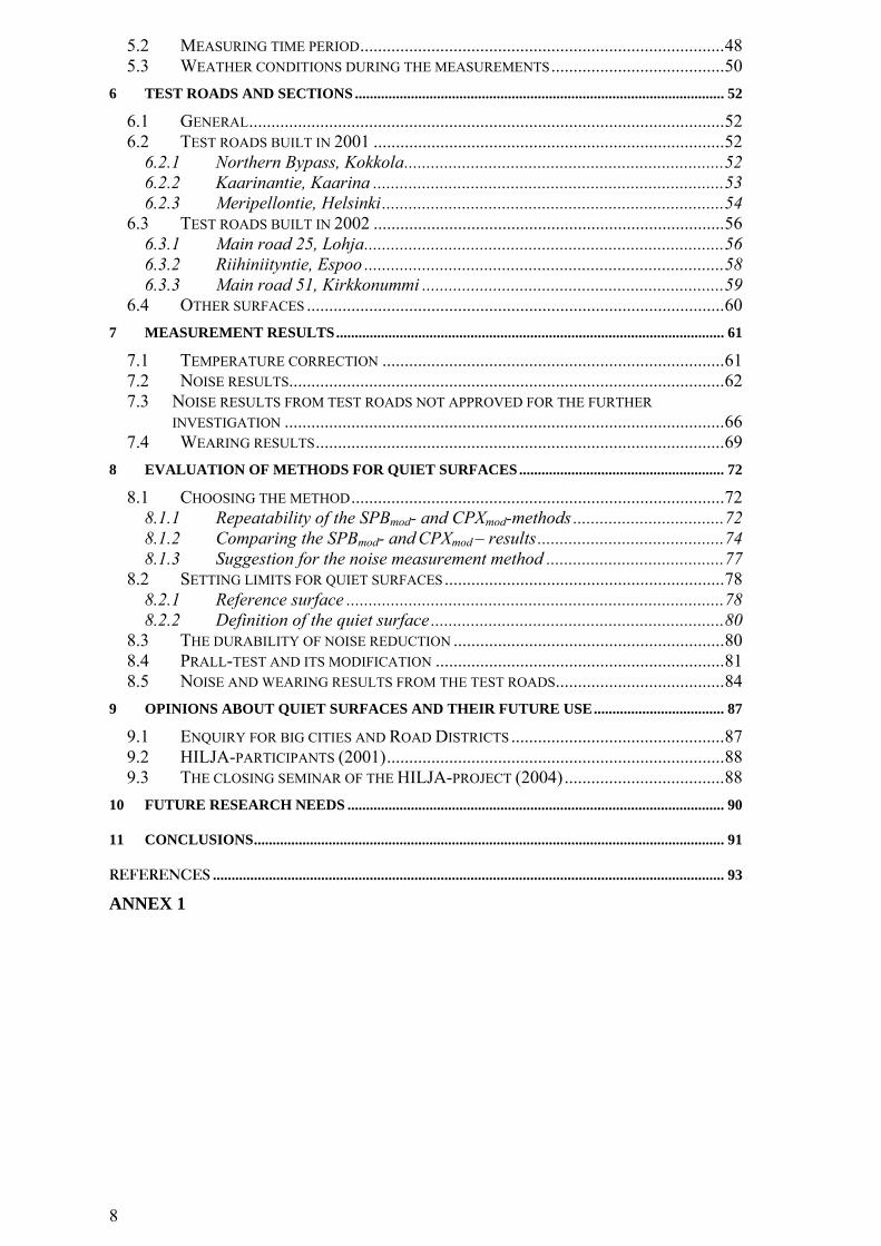
together give 43 dB at that point. The following figure (Fig. 2) gives the increase in sound level due to additional, equal sources.

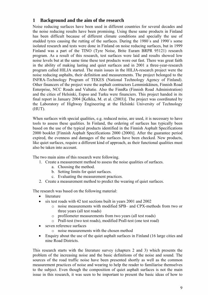
Figure 2: Addition of equal sound sources [Rossing, T. et al. (2002)] When putting this the other way around, it means that when the traffic for example decreases by half, the sound pressure level will decrease by 3 dB. This is a change which a human being can observe. However, when a person subjectively feels that there is a 50 % reduction in noise, this requires that the sound pressure level has decreased approximately by 10 dB. This would be equal to 90 % less traffic (Fig. 3). [Lahti, T. (2003)]

Figure 3: When the traffic decreases by half the sound pressure level will decrease by 3 dB. When a person subjectively feels that there is 50 % less noise, this requires that the sound pressure level has decreased by 10 dB which equals 90 % less traffic. [Lahti, T. (2003)]

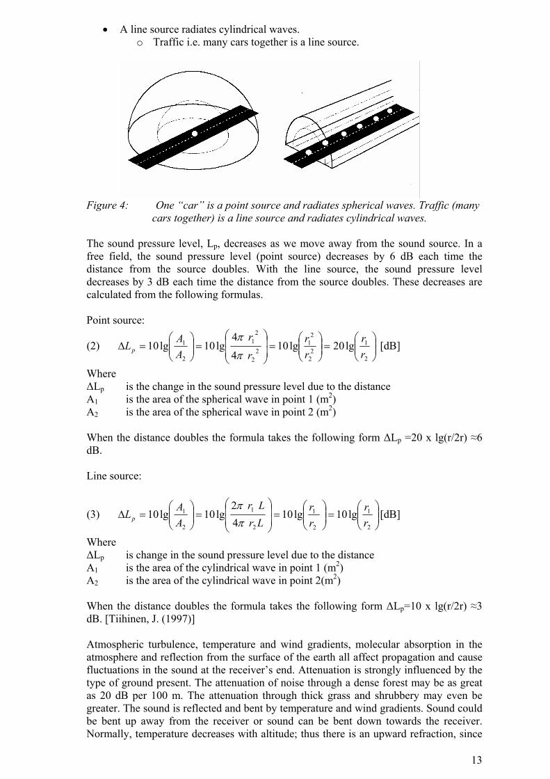
2.1.2 Sound propagation and suppression The source of the sound radiates a sound wave. The sound wave spreads out to a wider area when the distance increases. The noise gets muffled despite the environment. The sound can spread in different ways depending on the source (Fig.4).

• A point source radiates spherical waves. o For example a single car is a point source.

13

• A line source radiates cylindrical waves. o Traffic i.e. many cars together is a line source.

Figure 4: One “car” is a point source and radiates spherical waves. Traffic (many

cars together) is a line source and radiates cylindrical waves.

The sound pressure level, Lp, decreases as we move away from the sound source. In a free field, the sound pressure level (point source) decreases by 6 dB each time the distance from the source doubles. With the line source, the sound pressure level decreases by 3 dB each time the distance from the source doubles. These decreases are calculated from the following formulas. Point source:

(2) ⎟⎟⎠

⎞⎜⎜⎝

⎛=⎟⎟

⎠

⎞⎜⎜⎝

⎛=

⎟⎟

⎠

⎞

⎜⎜

⎝

⎛=⎟⎟

⎠

⎞⎜⎜⎝

⎛=∆

2

12

2

21

22

21

2

1 lg20lg104

4lg10lg10

rr

rr

r

rAA

Lp π

π [dB]

Where ∆Lp is the change in the sound pressure level due to the distance A1 is the area of the spherical wave in point 1 (m2) A2 is the area of the spherical wave in point 2 (m2) When the distance doubles the formula takes the following form ∆Lp =20 x lg(r/2r) ≈6 dB. Line source:

(3) ⎟⎟⎠

⎞⎜⎜⎝

⎛=⎟⎟

⎠

⎞⎜⎜⎝

⎛=

⎟⎟

⎠

⎞

⎜⎜

⎝

⎛=⎟⎟

⎠

⎞⎜⎜⎝

⎛=∆

2

1

2

1

2

1

2

1 lg10lg1042

lg10lg10rr

rr

LrLr

AA

Lp ππ

[dB]

Where ∆Lp is change in the sound pressure level due to the distance A1 is the area of the cylindrical wave in point 1 (m2) A2 is the area of the cylindrical wave in point 2(m2) When the distance doubles the formula takes the following form ∆Lp=10 x lg(r/2r) ≈3 dB. [Tiihinen, J. (1997)] Atmospheric turbulence, temperature and wind gradients, molecular absorption in the atmosphere and reflection from the surface of the earth all affect propagation and cause fluctuations in the sound at the receiver’s end. Attenuation is strongly influenced by the type of ground present. The attenuation of noise through a dense forest may be as great as 20 dB per 100 m. The attenuation through thick grass and shrubbery may even be greater. The sound is reflected and bent by temperature and wind gradients. Sound could be bent up away from the receiver or sound can be bent down towards the receiver. Normally, temperature decreases with altitude; thus there is an upward refraction, since

14

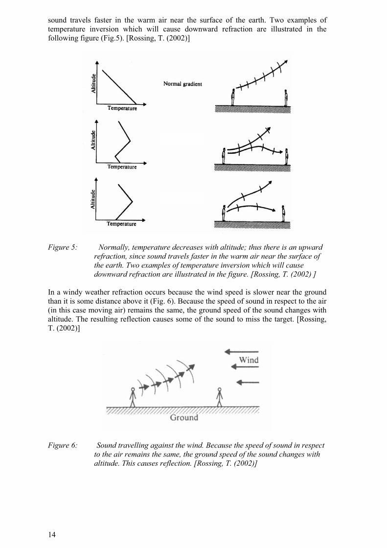
sound travels faster in the warm air near the surface of the earth. Two examples of temperature inversion which will cause downward refraction are illustrated in the following figure (Fig.5). [Rossing, T. (2002)]

Figure 5: Normally, temperature decreases with altitude; thus there is an upward refraction, since sound travels faster in the warm air near the surface of the earth. Two examples of temperature inversion which will cause downward refraction are illustrated in the figure. [Rossing, T. (2002) ]

In a windy weather refraction occurs because the wind speed is slower near the ground than it is some distance above it (Fig. 6). Because the speed of sound in respect to the air (in this case moving air) remains the same, the ground speed of the sound changes with altitude. The resulting reflection causes some of the sound to miss the target. [Rossing, T. (2002)]

Figure 6: Sound travelling against the wind. Because the speed of sound in respect to the air remains the same, the ground speed of the sound changes with altitude. This causes reflection. [Rossing, T. (2002)]

15

2.1.3 Frequency and A-weighting Frequency describes the speed at which the air pressure density variations or oscillations occur. It describes the number of full oscillations (periods) per second. The length of one period (in meters) is called wavelength. The unit of frequency is hertz [Hz] and 1 Hz is one oscillation per second.

(4) λcf = [Hz]

Where

f is frequency c is the speed of sound (345 m/s) λ is wavelength (m)

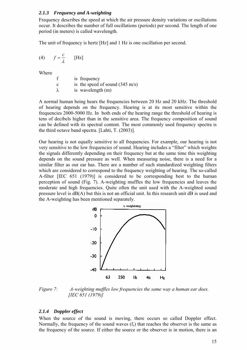
A normal human being hears the frequencies between 20 Hz and 20 kHz. The threshold of hearing depends on the frequency. Hearing is at its most sensitive within the frequencies 2000-5000 Hz. In both ends of the hearing range the threshold of hearing is tens of decibels higher than in the sensitive area. The frequency composition of sound can be defined with its spectral content. The most commonly used frequency spectra is the third octave band spectra. [Lahti, T. (2003)]. Our hearing is not equally sensitive to all frequencies. For example, our hearing is not very sensitive to the low frequencies of sound. Hearing includes a “filter” which weights the signals differently depending on their frequency but at the same time this weighting depends on the sound pressure as well. When measuring noise, there is a need for a similar filter as our ear has. There are a number of such standardized weighting filters which are considered to correspond to the frequency weighting of hearing. The so-called A-filter [IEC 651 (1979)] is considered to be corresponding best to the human perception of sound (Fig. 7). A-weighting muffles the low frequencies and leaves the moderate and high frequencies. Quite often the unit used with the A-weighted sound pressure level is dB(A) but this is not an official unit. In this research unit dB is used and the A-weighting has been mentioned separately.

Figure 7: A-weighting muffles low frequencies the same way a human ear does. [IEC 651 (1979)]

2.1.4 Doppler effect When the source of the sound is moving, there occurs so called Doppler effect. Normally, the frequency of the sound waves (fs) that reaches the observer is the same as the frequency of the source. If either the source or the observer is in motion, there is an

16

exception. If they are moving towards each other, the observed frequency is greater than fs. If they are moving apart, the observed frequency is lower than fs. This frequency shift is called the Doppler effect.

2.1.5 Maximum and equivalent sound pressure levels A common way to measure the sound level is to measure the A-weighted maximum sound level, LAmax. When measuring the passing vehicles, the maximum level is reached when the vehicle is at its closest point to the microphone. The sound pressure level which changes over the time can be described with one figure: equivalent sound pressure level (LAeq). This is not an average of the sound. LAeq is the constant sound level which for a certain time gives the same energy as the actual time history for the sound to be measured. The equivalent sound pressure level (LAeq) is calculated in the following way:

(5) ( ) dtp

tptt

Lt

t

AAeq ∫−

×=2

1

20

2

12

)(1lg10 [dB]

Where LAeq is A-weighted equivalent sound pressure level

t1 is starting time of the integration t2 is stopping time of the integration p(t) is sound pressure (Pa) p0 is reference sound pressure (20 µPa)

The sound changes during the time. For measuring the changing sound, different time periods have been standardized. The most commonly used time constants are “fast F” and “slow S”. The F time constant is 0.0125s and the S time constant is 1s. The shorter the time constant, the faster the measured sound level following the real changes of the sound level. The most commonly used time constant when measuring road traffic is fast (F).

2.2 Noise problem It has been estimated that around 20 percent of the population or close to 80 million people in the European Union (excluding new member states) suffer from noise levels which scientists and health experts consider unacceptable: most people become annoyed, their sleep is disturbed and adverse health effects are to be feared. An additional 170 million citizens are living in so-called “grey areas” where the noise levels are such as to cause serious annoyance during daytime. A wide variety of studies have examined the question of the external costs of noise to society, especially traffic noise. The estimates vary from 0.2% to 2% of gross domestic product. [EU (2004)] Because of this legislation and the technological progress, significant reductions of noise from individual sources have been achieved. For example, the noise from individual cars has been reduced by 85% since 1970 and the noise from lorries by 90%. However, data covering the past 15 years does not show significant improvements in the exposure to environmental noise, especially road traffic noise. The growth and spread of traffic in space and time and the development of leisure activities and tourism have partly offset the technological improvements. The forecast road and air traffic growth and the expansion of high speed rail risk exacerbating the noise problem. [EU (1996)] In 1998, a national survey about people exposed to noise was carried out in Finland. As a result, it was estimated that about every fifth person in Finland is exposed to

17

environmental noise in excess of 55 dB. The major source of this noise are the roads. About 880 000 people suffer from the noise of road traffic. This equals about 17% of the inhabitants. [Survo, K. et al. (1998)] In 2002, it was estimated that the situation has remained about the same. [Ympäristöministeriön moniste 102 (2002)]. Noise affects human beings in many ways. The most serious effect is loss of hearing, both temporary and permanent. Environmental noise is not usually at a level (sound pressure and frequency) that would cause a hearing loss. [Lahti, T. (2003)] However, environmental noise can still cause health problems. The most serious problem is that noise disturbs sleeping. Good and sound sleep is a basic need for the health of a human being. Noise can shorten sleep by making it difficult to fall asleep or it can wake people up. Noise can also affect the soundness of sleep even if the person does not wake up. The quality of sleep is weakened and the person wakes up easiest in the earlier hours when the sleep is not so sound. In both cases immediate physiological effects can be seen and they can cause health problems in a long run. Noise affects the activity of the brain, the heart beat and breathing of a sleeping person. The first effects can be seen when there are short peaks in the noise exceeding 40 dB. When these noise events increase, the risk of disturbance increases and the threshold of waking up is low when there are about five or more events where the maximum sound level exceeds 45 dB. [Lahti, T. (2003)] Some general conclusions can also be drawn about the effect of noise on performance. Steady noise below about 90 dB does not seem to affect performance but intermittent noise can be disruptive. Noise around 1000 to 2000 Hz is more disruptive than low-frequency noise. Noise is more likely to reduce the accuracy of work than to reduce the total quantity of it. Noise also appears to interfere with the ability to judge the passage of time. There is also a general feeling that nervousness and anxiety are caused by exposure to noise or at least are intensified by it. [Rossing, T. (2002)] Noise affects many normal activities in life. Both the hearing of speech and speaking itself becomes difficult when noise increases enough (Fig.8).

Figure 8: Maximum distance (outdoors) over which speech communication is possible. [Rossing, T. et al (2002) ]

18

Noise also affects many of our activities at home. Noise reduces enjoyment of a balcony or a garden and when inside, it interferes reading, watching TV or listening to music or radio.

2.3 Legislation affecting the environmental noise The most important law concerning the environmental noise is the Environmental protection law [Ympäristönsuojelulaki (86/2000)]. This law repealed the previous Noise protection law but the government decisions given by the Noise protection law stayed in force. One of the main decisions is presented in the following table. Table 1: Limits for the equivalent, A-weighted, sound level (LAeq) outside and inside

buildings. [Valtioneuvoston päätös (993/1992)] Outside LAeq(7.00-22.00) LAeq(22.00-7.00) Residential areas, recreation areas inside and near communities, areas for nursing homes and schools.

55 dB 45-50 dB 1) 2)

Holiday residential areas, camping sites, recreation areas outside communities and nature conservation areas

45 dB 40 dB 3) 4)

Inside Houses, nursing rooms, accommodation rooms 35 dB 30 dB School rooms and meeting rooms 35 dB - Business premises and offices 45 dB -

1) New areas, during the night time 45 dB 2) School areas do not have a limit for the night time 3) Nature conservation areas which are not used commonly for stay or for night time observation 4) Holiday living in the communities can be treated as permanent living The second important law in noise protection is the Land use and building law [Maankäyttö ja rakennuslaki (132/1999)]. This law sets the guidelines for all building, planning and land use. The aim is to build a healthy, secure and comfortable environment for living and working. The third important law is the law for Environmental assessment [Laki ympäristönvaikutusten arvioinnista (468/1994)] which orders that all major projects including motorways have to be assessed. In this assessment, noise has to be taken into consideration. The Road traffic law [Tieliikennelaki (267/1981)] and the statute for vehicles construction and equipment [Asetus ajoneuvojen rakenteesta ja varusteista (530/1993)] contain regulations for the noise emissions of vehicles. There are also other laws which have an indirect effect on noise protection but those mentioned above are the most important and set the limits for road traffic and its noise emissions. The European Union has set legislation on the noise emission of products. These are for example the maximum permissable noise emission for new vehicles [Directive 1996/20/EC] and the maximum permissable noise emission for new tyres [Directive 2001/43/EC]. In 2002, a directive about the assessment and management of environmental noise was published [Directive 2002/49/EC]. This directive introduces common noise indicators Lden (indicator of the overall noise level during the day, evening and night) and Lnight (indicator for the sound level during the night). It also stipulates that the Member States have to provide strategic noise maps.

19

2.4 Road traffic noise and its controlling There are many factors which affect road traffic noise. They can be divided into three different groups: • vehicle type and composition (personal car, truck, motorcycle) • road and traffic flow • driving behaviour. The noise of the vehicle originates mainly from the following sources: • power unit

• fan, engine, exhaust, transmission • tyre/road interaction • wind turbulence. The power unit noise, tyre/road noise and wind turbulence noise have different importance in the total noise emission in different speeds. Both tyre/road and power unit noise have a strong relationship with vehicle speed. The tyre/road noise level increases approximately logarithmically with speed, which means that on a logarithmic speed scale, noise levels increase linearly with speed. The power unit noise depends on a number of vehicle operating factors, most notably the gear selection and the engine speed, and its relation with vehicle speed is much more complicated than that of tyre/road. At low speeds, the power unit noise dominates while at high speeds the tyre/road noise dominates, and there is a certain “crossover speed” where the contribution is about the same. Since we know that if one has two noise sources which are equally strong, the overall level will be 3 dB higher than the level for the single source, we can say that the power unit noise level equals tyre/road noise when the overall noise is 3 dB higher than tyre/road noise; if it is less than 3 dB higher, tyre/road noise will dominate. [Sandberg, U. (2001)]. According to Sandberg´s research the tyre/road noise dominates over the power unit noise with passenger cars for all speeds and gears except when driving on the first gear. In practice, it means that when driving at a constant speed, tyre/road noise always dominates, even at low (30 km/h) speeds and in congested urban situations. [Sandberg, U. (2001)] When vehicles are under acceleration, both tyre/road and power unit noise levels increase due to the extra tyre torque and engine load; the increases are normally highest for the power unit noise. This means that at such conditions the power unit noise may occasionally exceed the tyre noise. [Sandberg, U. (2001)] With heavy vehicles, the power noise dominates during all accelerations 0-50 km/h, but the tyre /road noise dominates at all driving above 50 km/h and already from about 40 km/h at a constant speed. [Sandberg, U. (2001)] The tyre/road noise has a crossover speed after which it starts to dominate over the power unit noise as stated above. This crossover speed is not constant but it depends on many factors like the type of the vehicle, load and model year. The third component of the total vehicle noise is the wind turbulence noise. The aerodynamic design of vehicles is necessary for meeting the consumption requirements. This has meant that the wind turbulence does not cause much exterior noise, however it has an effect on the interior noise. [Sandberg, U. et al. (2002)] In reality, this noise factor is important for the exterior noise only at really high speeds like for example speeds of high-speed trains. These speeds and the wind turbulence noise are not important at everyday car traffic speeds. [Lahti, T. (2003)]

20

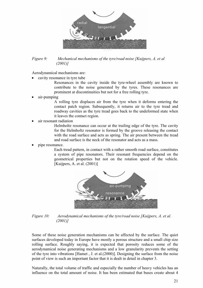
The main power unit noise source in motor vehicles is the combustion or explosion of the fuel-air mixture inside the cylinders. This very powerful noise source is buried deep inside the massive engine and therefore is well attenuated. Some of the energy of combustion does appear as noise, however, due to vibration of the entire engine as well as individual parts. Furthermore, when the exhaust and intake valves open, loud sound of short duration are emitted, especially in the exhaust system, since the exhaust valve opens when the cylinder pressure is still quite high. Engine cooling fans produce also a substantial amount of noise.[Rossing, T. (2002)] The tyre/road noise depends on many factors, for example: • model and age of the vehicle • axle weight • tyre pressure • tyre type (summer/ winter tyre, studded tyre) • size of the tyre • temperature of the tyre • tyre texture and material • road surface, its quality and temperature. [Sainio, P. (2000)] The generation of the tyre/road noise is a complicated phenomenon which is not fully known. There are dozens of different generation mechanisms and their mutual share of the total tyre/road noise depends on the surface, tyre and its texture as well as on the speed of the vehicle. In general these generation mechanisms can be divided into two groups: mechanical (Fig.9) and aero dynamical (Fig. 10) mechanisms. Mechanical mechanisms are: • radial and tangential vibrations of the tyre

Radial vibrations of the tyre belt and of the profile elements are excited by road roughness elements deforming the tread or by tread elements hitting (on the leading edge) or leaving (on the trailing edge) the road surface. Tangential vibrations are excited by tangential forces in the contact patch.

• side wall vibrations The tread vibrations are transported to the side wall which acts as a “sounding board” and radiates sound.

• stick-slip Stick-slip vibrations are a result of the stick-slip phenomenon which occurs when materials exhibit reduced friction with an increase in their relative speed. So the tread blocks of the tyre alternately “stick” and “slip” relative to the road surface. This mechanism is normally associated with situations where relatively high tangential forces are applied to the tyre.

• adhesion stick-snap. Stick-snap occurs when the tyre tread surface gets sticky and the road surface is very clean. The adhesive bond strength is increased, which leads to an increase of the excitation at the trailing edge of the tyre footprint. [Kuijpers, A. et al. (2001)]

21

Figure 9: Mechanical mechanisms of the tyre/road noise [Kuijpers, A. et al

(2001)] Aerodynamical mechanisms are: • cavity resonance in tyre tube

Resonances in the cavity inside the tyre-wheel assembly are known to contribute to the noise generated by the tyres. These resonances are prominent at discontinuities but not for a free rolling tyre.

• air-pumping A rolling tyre displaces air from the tyre when it deforms entering the contact patch region. Subsequently, it returns air to the tyre tread and roadway cavities as the tyre tread goes back to the undeformed state when it leaves the contact region.

• air resonant radiation Helmholtz resonance can occur at the trailing edge of the tyre. The cavity for the Helmholtz resonator is formed by the groove releasing the contact with the road surface and acts as spring. The air present between the tread and road surface is the neck of the resonator and acts as a mass.

• pipe resonance. Each tread pattern, in contact with a rather smooth road surface, constitutes a system of pipe resonators. Their resonant frequencies depend on the geometrical properties but not on the rotation speed of the vehicle. [Kuijpers, A. et al. (2001)]

Figure 10: Aerodynamical mechanisms of the tyre/road noise [Kuijpers, A. et al. (2001)]

Some of these noise generation mechanisms can be affected by the surface. The quiet surfaces developed today in Europe have mostly a porous structure and a small chip size rolling surface. Roughly saying, it is expected that porosity reduces some of the aerodynamical noise generating mechanisms and a low granularity prevents the setting of the tyre into vibrations [Hamet , J. et al.(2000)]. Designing the surface from the noise point of view is such an important factor that it is dealt in detail in chapter 3. Naturally, the total volume of traffic and especially the number of heavy vehicles has an influence on the total amount of noise. It has been estimated that buses create about 4

22

dB, trucks about 6 dB and articulated trucks about 9 dB more noise than passenger vehicles [Eurasto, R. (2002)]. Other factors in road design causing extra noise are for example crossings, longitudinal slope falls, curves and other places which cause drivers to change gear, accelerate or decelerate. The crossings usually break the free traffic flow. Their design and signalling affect the noise. A green wave in traffic lights and traffic lights reacting to the vehicles closing affect the noise of the crossings a little. A green wave reduces noise less than 2 dB but a “red wave” can increase it more. Roundabouts increase noise about 1-2 dB when the increase of the “normal” crossing is about 2-4 dB. [Lahti, T. (2003)] Other traffic controlling systems calming the speed also reduce noise in theory. These include speed limits and installation of road humps. It must be noticed that these installations causing strong acceleration or decelerating can actually produce more noise or the noise reduction does not occur. The altitude of the road also affects the spreading of noise. A road that is higher than the surrounding area spreads the noise over a larger area than a road at the same or lower level as its surroundings. The reducing of speed has a strong effect on noise. When measuring the LAmax with the SPB-method (see chapter 4) the following reductions (Table 2) can be achieved in theory. It must be noted that lowering the speed limit does not automatically reduce the noise if these limits are not controlled and, on the other hand, reducing speed can cause reduction in the trafficapability and break the free flow. Table 2: Noise reductions ( LAmax, SPB-method) when reducing speed. [Sandberg, U. et

al. (2002)] Speed reduction [km/h] Noise reduction [dB]

80→ 60 4.4 60→ 50 2.8 60→ 40 6.2 50→ 40 3.4 50→ 30 7.8 40→ 30 4.3

Even within any vehicle type, the noise generated by an individual vehicle is significantly affected by how the vehicle is driven. Specifically, the noise emitted depends upon the operating speed of the vehicle, the gear selected and whether the vehicle is accelerating or decelerating. These factors have a constantly varying influence on the traffic noise as drivers attempt to cope with the traffic and road conditions encountered as part of normal driving. However, no two drivers will react in exactly the same way to a given situation, as driving styles are known to differ substantially. [Phillips, S. (2001)] Up till now the road traffic noise problem has generally been solved by building noise walls or embankments. Traditional noise abatements can not be used in all environments. Noise walls and banks are useful in open environment and outside cities. Town planning can also be used in new areas. Window and facade isolations have been used in building constructions for noise reduction. Quite often inside cities and in suburban areas it is not possible to build massive constructions to protect the inhabitants from noise and these big constructions do not always fit into the surrounding environment and meet its beauty requirements. Quite often there is not enough space and these constructions also restrict the view of the inhabitants and are exposed to violence. It is not possible to compare the costs of quiet surfaces and other noise abatement methods in this research as prices as well as operating life spans of the surfaces are not

23

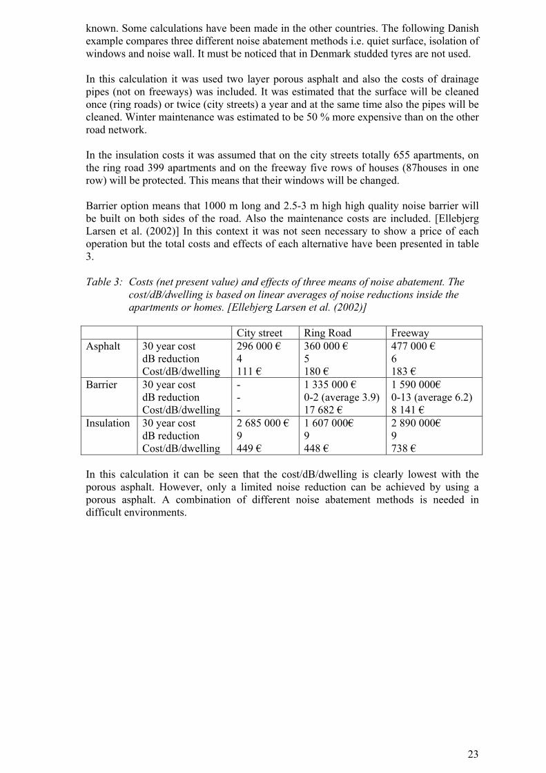
known. Some calculations have been made in the other countries. The following Danish example compares three different noise abatement methods i.e. quiet surface, isolation of windows and noise wall. It must be noticed that in Denmark studded tyres are not used. In this calculation it was used two layer porous asphalt and also the costs of drainage pipes (not on freeways) was included. It was estimated that the surface will be cleaned once (ring roads) or twice (city streets) a year and at the same time also the pipes will be cleaned. Winter maintenance was estimated to be 50 % more expensive than on the other road network. In the insulation costs it was assumed that on the city streets totally 655 apartments, on the ring road 399 apartments and on the freeway five rows of houses (87houses in one row) will be protected. This means that their windows will be changed. Barrier option means that 1000 m long and 2.5-3 m high high quality noise barrier will be built on both sides of the road. Also the maintenance costs are included. [Ellebjerg Larsen et al. (2002)] In this context it was not seen necessary to show a price of each operation but the total costs and effects of each alternative have been presented in table 3. Table 3: Costs (net present value) and effects of three means of noise abatement. The

cost/dB/dwelling is based on linear averages of noise reductions inside the apartments or homes. [Ellebjerg Larsen et al. (2002)]

City street Ring Road Freeway Asphalt 30 year cost

dB reduction Cost/dB/dwelling

296 000 € 4 111 €

360 000 € 5 180 €

477 000 € 6 183 €

Barrier 30 year cost dB reduction Cost/dB/dwelling

- - -

1 335 000 € 0-2 (average 3.9) 17 682 €

1 590 000€ 0-13 (average 6.2) 8 141 €

Insulation 30 year cost dB reduction Cost/dB/dwelling

2 685 000 € 9 449 €

1 607 000€ 9 448 €

2 890 000€ 9 738 €

In this calculation it can be seen that the cost/dB/dwelling is clearly lowest with the porous asphalt. However, only a limited noise reduction can be achieved by using a porous asphalt. A combination of different noise abatement methods is needed in difficult environments.

24

3 Quiet asphalt surfaces and their measuring

3.1 What is a quiet asphalt surface? How quiet should a surface be to be defined quiet? This is a question without one single or scientific answer but it is a question of personal appreciation. How much is enough and how can the noise reduction be shown? The noise reduction can be defined for example by measuring the noise before and after repaving the road with a noise reducing surface. Another way would be to compare the measured noise with a noise of a commonly used surface. An advantage of the second alternative is that it assesses the surfaces in different areas the same way. For example, Ulf Sandberg and Jerezy A Ejsmont define a quiet surface the following way: “ “A low noise road surface” is a road surface which, when interacting with a rolling tyre, influences vehicle noise in such a way as to cause at least 3 dB(A) (half power) lower vehicle noise than that obtained on conventional and “most common” road surfaces”. [Sandberg, U. et al. (2002)] This definition is for comparing A-weighted noise levels which can be measured either with the SPB- or CB-method. One of the tasks is to define these ”most common” reference surfaces which other surfaces will be compared to. Different countries can have different reference surfaces and they can change over the time. According to the ISO 11819-1 standard, the reference surface is a dense, smooth-textured asphalt concrete surface with a maximum chipping size of 11 mm to 16 mm. From the acoustical point of view, this is approximately equivalent to a stone-mastic asphalt surface with the same chipping size. When used as a reference surface it must have been trafficked for at least one year. The surface must be non-absorbing and the macro texture must be within 0.5-1.0 mm. The reference surface could also be fictitious. It can be for example based on the average results of a great number of SPB-measurements on the earlier mentioned surfaces. [ISO 11819-1] The ISO 10844 standard [ISO 10844 (1991)] also introduces a reference surface but this surface is used for tyre testing where the surface factor must be standard. In the United Kingdom a special system has been developed for assessing surfaces. The SPB-method has been incorporated into the noise test provided within the Highway Authorities Product Approval Scheme (HAPAS) for the approval or certification of road surfacing products for use on public roads in the U.K. The HAPAS procedure combines the results of SPB-measurements into the expected level of noise arising from a typical trunk road or alternatively a specified class of local road. From this value is subtracted the noise level that the standard noise calculation produces for the same traffic flow assuming the road had an average conventional surface. This difference is called the Road Surface Influence. [Highway Agencies (2002)] In principle, only approved products may be used without restrictions on trunk roads and motorways in the U. K. No official limits have been set and the noise test currently gives information when procurement is made. However, some agencies have set their own limits. For example, for certain exposure situations, the Highway Agency has specified guidelines for determining the types of materials that may be used based upon their HAPAS noise levels. [Sandberg, U. et al. (2002)] In the HAPAS system a “low noise surfacing” has been one that is 2.5 dB quieter than the reference type. The latter is formally the reference surface in CRTN (Calculation of Road Traffic Noise [UK DoT (1988)]) . In reality, this is “normal” hot rolled asphalt with about 20 mm chipping size. [Sandberg, U. et al. (2002)]

25

3.2 What makes surfaces quiet

3.2.1 Types of the quiet surfaces A conventional asphalt concrete consists of • aggregates

• crushed stones of size 2-16 mm • sand of size 0.063-2 mm • filler, very fine sand of size <0.063 mm

• binder, typically bitumen • possible additives (fibres, polymers, rubber etc.). The mixture of these is laid on the road and the surface gets its final composition depending on its compaction and laying conditions. The voids ratio of the final asphalt layer varies as well as its texture. The voids ratio of a dense asphalt concrete is typically <5 % of the volume. There are many surface characteristics known or believed to affect traffic noise emission. Their importance varies. Some are more important for noise reduction than others. Some of the characteristics are:

• texture of the surface • porosity • thickness of the layer • tyre/road adhesion • elasticity of the surface • colour of the surface.

Some of these characteristics are presented in detail later in this chapter. Roughly speaking, there are two main types of quiet surfaces which are:

• non–porous surface • porous surface.

In the non-porous surfaces the noise reduction is usually achieved by smoothening the surface texture. This can be achieved, for example, by limiting the maximum grain size or by extra compacting. Porous surfaces exhibit three major properties of importance to vehicle noise reduction: 1. Its porosity will eliminate the compression and expansion of air entrapped in the

tyre/road interface when tires are rolling over the surface. “Air-pumping and air resonant tire noise” will be reduced.

2. Porosity will also reduce the amplifying effect of the acoustical horn existing in the space between the curved tire tread and the plane road surface. [Sandberg, U. (1999)]

3. The noise benefits are partly dependent upon the complex interference which occurs between acoustic waves which propagate directly from the vehicle source to the receiver and waves which are reflected from the road surface. When the source and receiver of the noise are close to the ground, reflections from the ground plane will occur. To determine the acoustic field strength at the receptor it is necessary to determine the phase and amplitude of the direct and reflected waves and then combine these components taking account of any phase interactions (i.e. interference) that occur. With the porous surfaces, destructive interference will generally occur in the frequency range 250-1000 Hz (Fig. 11). [Nelson, P.M. (1994)]

26

Figure 11: Geometry for a source and receiver in the vicinity of a ground plane.

[Nelson, P.M. (1994)] Smoothening the surface of the porous asphalt is as important as with the non-porous quiet surfaces. This will emphasise the effect of the porous. Anyhow, it is important to find the balance between the porosity and the smoothness of the texture. A too small maximum grain size can, for example, reduce the porosity and too much rolling will reduce the porosity as well. [Sandberg, U. (1999)] The advantage of porous surfaces is that they reduce both the tyre/road noise and the power unit noise of the vehicles. To strengthen this effect, not only the driving lanes should be paved with porous surfaces but also the road shoulders, sidewalks and car parks. As large areas as possible between source and receiver, even outside the road lanes, should be covered with porous material in order to make use of the absorption of propagating sound. [Sandberg, U. (1996)]

3.2.2 Texture of the surface The road texture differs from the mean plane of the surface. The texture can be described by two parameters: amplitude (vertical deviation) and wavelength (horizontal periodicity). Texture is defined in three ranges (Fig. 12): • micro texture (texture having wavelengths of 0.5 mm and less)

This is the region of the texture spectrum which is associated with the small scale roughness of stones. It is responsible for the adhesion component of friction between the tyre and road surface.

• macro texture (texture having texture wavelengths between 0.5 and 50 mm) Macro texture is important by helping to disperse surface water by providing drainage channels in the surface. The macro texture is obtained by suitable proportioning of the aggregate and mortar of the surface or by surface finishing techniques.

• mega texture (texture having texture wavelengths between 50 and 500 mm). Mega texture is often materialized as potholes or “waviness”. It is usually an unwanted characteristic and it has a harmful effect both for friction and noise. [Chavet, J. et al. (1987)] [Nelson, P. et al. (1997)]

27

Figure 12: Micro-, macro, and megatexture and their influence on different

functions of the surface. [Chavet; J. et al. (1987)] The micro texture has a small effect on noise reduction. Polished surfaces should be avoided which means that polish-resistant materials should be used. A polished surface seems to give stronger adhesion bonds in dry condition than a non-polished one with a “rugged” micro texture and this seems to give somewhat higher noise. [Sandberg, U. (1996)] In Finland and in other countries where studded tyres are used, polishing does not play a major role because in winter surfaces get rough again. Crushed stones with sharp edges resist polishing and should be preferred. At the same time sharp edges cause higher amplitudes of high frequency components than a similar waveform without such sharp edges. In the wavelength range of 1-8 mm high amplitudes mean low noise. This leads us to the issue of macro texture. Optimizing the macro texture plays an important role in noise reduction. There are some major issues which should be optimized. Light vehicles: • Macro texture should have high amplitudes in the 1-8 mm wavelength range. • Macro texture should have low amplitudes in the 10-50 mm wavelength range. Heavy vehicles • Macro texture should have high amplitudes in the 0,5-12 mm wavelength range. • Macro texture should have low amplitudes in the 16-50 mm wavelength range. [Sandberg, U. (1996)] There is one problem because there is an intercorrelation (correlation coefficient 0.7-0.9) between texture at different wavelengths such as 5 and 50 mm. This means that a surface with high texture at 50 mm usually also has it at 5 mm and vice versa. The practical problem is to force a texture to be high at 5 mm without increasing it also at 50 mm.

28

However, by the choice of chipping size and shape, one can tailor the texture spectrum to a considerable degree. [Sandberg, U. (1996)] The larger the chipping size, the worse it is from the noise point of view. The maximum size should not exceed 8 mm (12 mm when optimizing the noise from heavy vehicles) but 4-6 mm (6-10 mm, heavy vehicles) would be even better. In all cases chipping sizes larger than 10 mm (12 mm, heavy vehicles) should be avoided. [Sandberg, U. (1996)] There is a conflict between these requirements. When selecting a small maximum chipping size, the amplitude will also be lower since the amplitude is often roughly proportional to the chipping size. Smaller chippings mean lower amplitude in the important 1-8 mm wavelength range but they also mean lower amplitude in the range over 10 mm which may be even more important. If the choice between these requirements should be made, the small chipping size should be preferred. [Sandberg, U. (1996)] Choosing the smaller chipping size is recommended purely from the noise point of view. In areas where studded tyres are used also the wearing must be taken into account when choosing the chipping size. A rough mega texture generates low frequency noise. The general advice is that mega texture should be minimized. This can be reached by avoiding the large chipping size, and the macro texture should be homogenous. Otherwise “missing chips” or large spaces between the chippings cause the mega texture to increase. This can be avoided the following ways: • Chippings should be of uniform size and well packed together. • Cubical particle shape should be preferred. They will be easier packed and oriented

than for example chippings with high flakiness. • If flaky chippings are used, surface should be compacted well in order to get a

uniform orientation. [Sandberg, U. (1996)] Porous surfaces can be optimize by affecting on three factors: • texture-for lowest impact excitation to the tyres • porosity-for favourable drainage and sound absorption properties • thickness and number of layers. For porous surfaces, the lowest possible mega and macro texture at all wavelengths is desired. This means, among other things that the chippings need not to be sharp. When the porosity is high the effect of air drainage is achieved with the porous while it is obtained with non-porous surfaces through high texture amplitudes at short wavelengths. This is valid only as long as the surface is really porous. When a surface has reached a certain degree of clogging the surface obeys the same ways as non-porous surfaces. [Sandberg, U. (1996)] To get the lowest texture, chippings as small as possible should be used. However this is in some conflict with the requirements for void content and non-clogging properties. A compromise has been found in the double-layer surfacing in which a small chipping size is desirable in the top layer as long as the chippings are large below. [Sandberg, U. (1996)] Also soft aggregate should never be used together with hard one because the soft chippings will be worn quicker and leave spaces which will result in an unwanted mega– and macro texture. The worn-of particles will also fill the voids. [Sandberg, U. (1996)]

29

3.2.3 Porous When increasing porosity, it is important to find the right balance between noise reduction and the mechanical strength and durability of the surface. However, the surface will not be acoustically efficient until the air void content is >20 %. [Sandberg, U. (1996)] It seems that a porosity of 25-30% is the maximum that can be achieved for a mixture which still offers acceptable mechanical stability. [von Meier, A. (1992)] The design goal is to obtain the maximum amount of sound absorption (α =1) at the frequency of fαmax =1000 Hz for high speed roads and of f αmax =600 Hz for low speed roads. [von Meier, A. (1992)]

3.2.4 Binder and elasticity The effect of binder in reducing noise has not been fully researched. It has been noticed that the stiffer the surface is, the noisier it is. To be on the safe side, binders providing stiff surfaces should be avoided. On the other hand, it has not been noticed that binders including rubber powder would give any lower noise due to reduced stiffness. [Hamet; L. et al. (2000)] However, rubber granules used as a part of an aggregate have given promising results. In Japan, a poroelastic surface reduced noise by 10 dB when a similar surface without rubber granules gave 6 dB reduction. [Ohnishi, H (2002)]

3.2.5 Colour The colour of the surface can also influence its noisiness. A black surface absorbs the sunshine and can easily get 10 ºC warmer than a bright surface. It is known that one degree addition in the temperature equals about a 0.1 dB reduction in noise. (There is further discussion about the effect of temperature in chapter 3.4.3). This means that a dark surface could be about 1 dB quieter than a bright one.

3.2.6 The durability of the reduced noise The noise properties of the surfaces change over time. For some surface types, this change can be quite small, for other surfaces it may be dramatical. The following phenomena can cause loss of noise properties: • Mega– and macro texture are changed, as particles and other material are worn out. • Mega– and macro texture, as well as stiffness, are changed due to the surface

structure being compacted by traffic. • Micro texture is changed, mainly by a polishing effect of many tyres passing over

the surface (studs on tyres may counteract this effect). • The chemical effects of the weather, maybe assisted by road salt, result in the

weathering and crumbling of the surface (loss of fine material), affecting both micro texture and macro texture. Rain may also play a role in changing the micro texture.

• Cracks may occure. • If the surface is porous, its pores will become clogged by accumulated dirt. [Sandberg; U. et al. (2002)] General assumption is that for smooth, medium-textured dense asphalt surfaces noise levels generally increase during the first 1-2 years, then remain stable until the end of the lifetime several years later when severe mega texture, cracks and unevenness occur. For porous surfaces, porosity becomes clogged with dirt, some chippings may get lost creating a rougher texture and the initially smooth-rolled top part of the surface will “deteriorate”. This is a continuous process, sometimes reducing noise reduction properties very rapidly, sometimes not so rapidly. [Sandberg; U. et al. (2002)]

30

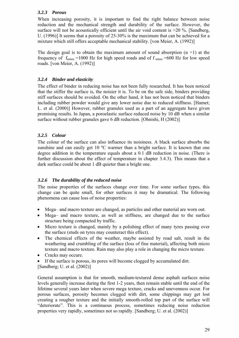
In Denmark it was noticed that the porosity is less clogged and the noise reduction stands longer on the wheel tracks than outside these tracks. Porous surfaces seem to have a self-cleaning mechanism. The more traffic and higher speeds, the better the self-cleaning is. [Bendtsen; H. (1998)] However, it must be noticed that this research was made in an environment where studded tyres are not used. In Finland, the situation can be different. In Denmark the long-term noise reduction of porous asphalt surfaces was researched. The products tested were (Fig.13): • dense asphalt concrete, max. particle size 12 mm (reference) • porous asphalt, max. particle size 8 mm, with pores 18-22 % • porous asphalt max. particle size 8 mm, with pores more than 22 % • porous asphalt max. particle size 12 mm, with pores more than 22 % • open graded asphalt concrete max. particle size 12. No cleaning of the surfaces was done. The first measurements were taken from the test sections in September 1990. Measurements were taken in a manner very similar to the Statistical pass-by. [Raaberg; J. et al. (2001)] It can be seen (Fig. 13) that the sections with porous asphalt were less noisy than the reference section (laid on the road at the same time) during the first six years. After seven years, the noise reduction disappears for all porous asphalt types. In figure 13, we can also notice that the reference surface gets noisier during the first two years and after that its noise qualities seem to become stable for the next five years. The old reference surface gets increasingly noisier throughout the whole test period.

Figure 13: Noise level on test sections at Viskinge, expressed as LAE values (dB) at

80 km/h, for an 8 year period. [Kragh, J. et al. (1997)]

3.3 Rutting of the quiet surfaces

3.3.1 General The rutting of surfaces consists of two different parts: a deformation during summer and a wear caused by studded tyres during winter.

70

72

74

76

78

80

82

84

0 1 2 3 4 5 6 7

Age

LAE

(80

km/h

, 10m

)

AC 8 18-22%

PA 8>22%

PA12>22%

AC 12(dense) ref.

AC 12 (open)

31

In Finland about 70-80 % of the rutting is wearing and only 20-30% is caused by deformation. [Ehrola, E. (1996)] The Finnish Road Enterprise ran a series of tests on its quiet asphalt product (HILTTI). One interesting result was that the deformation of quiet surfaces was only half of the deformation of SMA 16. Core samples were made for this research by the ICT (Intensive Compaction Tester) and the method used was PANK-4208 (cyclic compression test). [Komulainen, K. et al. (2002)] This result was confirmed in HILJA-research where the deformation of test surfaces was followed. [Kelkka, M. et al. (2003)] Deformation has not been researched further in this research. Studded tyres cause longitudinal ruts on the road. Ruts are formed when the studs either hit or scratch the surface. Ruts have a negative effect on traffic safety because the water staying in them increases the risk of aquaplaning. Fast wearing also increases the need to resurface. This means added costs and inconvenience to the traffic. Faster wearing also generates more dust into the air. The diameter of the dust particles originating from the wearing of asphalt surfaces is 2.5-10µm. These particles are unhealthy when breathed. Wearing is a typical problem in Finland because of the studded tyres used. About 88% of the winter tyres are studded. The share of friction tyres has been slowly increasing from 4 % (winter 1992-1993) to 12 % (winter 2000/2001). In contrast, over the same period of time, the use of friction tyres in vans fell from 11% to 6%. With steadily tightening requirements for a lower stud weight in Finland, the use of steel studs especially in passenger cars has decreased. During winter 1992-1993, the proportion of steel studs in passenger cars was 88% compared with 25% during winter 2000-2001. [ Malmivuo, M. et al.(2001)] The Ministry of Transport and Communications has expected that in the near future the rutting of Finnish main roads will increase 3 % annually even though the stud mass has decreased. This will be caused for example by the rising of tyre pressure and the mass of passenger cars as well as the rising of the driving speed. [Unhola, T. (2004)]

3.3.2 Experiences in Finland Early experiences with quiet surfaces in Finland have shown that rutting is a problem with quiet surfaces. As a result of the international TINO-project (Tyre Noise, Brite Euram, BRPR 950121) two test sections were built on Ring Road III in 1999. The tested products were SMA 5 and TINO (including light weight aggregate). After the first winter, these test sections were worn out. After this experience a large number of PWR-test were run in the Laboratory of Highway Engineering (HUT). The result was that these products wore out 2-3 times more than SMA 16. The light weight aggregate used in the TINO-surfaces particularly increased the wearing. [Valtonen, J. et al. (2000)] In 2000 and 2001 the wearing of some quiet surfaces was also measured on Ring Road I (Vallikallio) and Vantaa (Korso). The result of these measurements was that SMA 5 wore out six times faster than SMA 11 and ten times faster than SMA 16. [Hyyppä, I.. et al. (2001)] These early experiments in the 1990´s gave quiet surfaces a bad reputation and their use and development was stopped almost ten years.

32

3.3.3 Experiences in other countries The rutting of surfaces is a typical problem in Finland. Quiet asphalt products have been used widely in other countries where the wear caused by studded tyres is not a problem and that is why this problem has not been researched either. The problems with the resistance to wear have been caused by other things. For example, in the Netherlands it was reported that porous asphalts are not very resistant against heavy turning traffic. [Van, Bochove, G. (2000)] Also from Sweden and Norway, where studded tyres are used, there is only some information available. In Norway, some porous surfaces were followed from 1989 to 1994. They found out that abrasive wear caused by studded tyres seemed to be of minor importance. Other factors, like the loss of chippings seemed to reduce the life-span of quiet surfaces. It was noticed that the development of ruts depended much on the climatic conditions of winter, showing accelerated loss of chippings during the periods of rapid changes of frost and thaw. The same happened to dense asphalts as well but it was more moderate. The characteristic damage of porous surfaces seemed to be pot holes as a result of accelerated loss of chippings. [Norwegian Public Roads Administration (1994)] The other worry in Norway concerning the studded tyres seemed to be the fast clogging of porous not wearing. [Statens Vegvesen (2003)] A new interest to porous surfaces has risen in Norway and some test roads from the years 1996…2003 were measured by CPX. [Sintef (2004)] No information was found about the rutting of these surfaces. In Sweden the biggest problems with porous surfaces in the early 1990´s seemed to be the binder and its ageing and hardening. This caused the loosening of the stones. Today the Swedes do not see the rutting as a big problem because the aggregates are better and the development of binders has been significant in the 1990´s. [Wåberg, L-G (2004)] In 2003, three test sections were built on the E 18 motorway in Sweden. A special binder was used. [Relund, M (2003)] There was no exact information available about their rutting but it was estimated that the upper layer would last seven years and bottom layer 14 years. [www.trailer.se (2004)]

3.3.4 Surface properties affecting the wear The properties of asphalt surfaces were researched in the large ASTO-research program in 1987-1992. [PANK ry (1993)] After that research, there was quite a good understanding in Finland of the factors affecting the wearing of asphalt surfaces. In the following list these factors are shortly presented for the orientation of the reader.

• Aggregate Aggregate has the strongest effect on the wearing. Crushed aggregates used for surfaces have been divided to strength categories I-IV according to their Nordic abrasion value (SF-EN 1097-9). To secure the wearing, deformation and weather resistance properties of the surface also the < 8 mm aggregate has been crushed from the material fulfilling the criteria set. [PANK ry (2000)]

• Binder

The wearing properties of the surface can be improved little with the binder. Some special products like rubberised bitumen can resist wearing 10 per cent more than the “normal” products. The amount of binder does not affect the wearing remarkably. [PANK ry (1993)]

• Surface type

33

The most wearing surface types are those with a continuous grading curve and a small maximum grain size. Differences in wearing can be explained for example with an 8 mm passing and maximum grain size. [PANK ry (1993)]

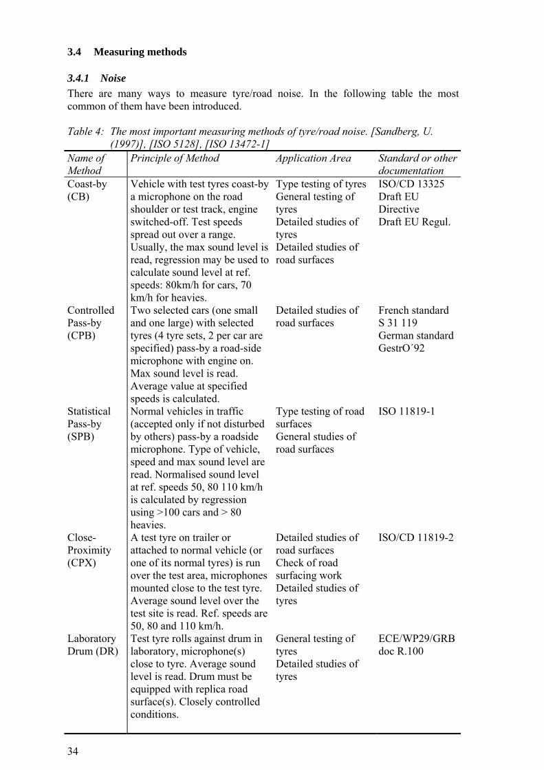
34

3.4 Measuring methods

3.4.1 Noise There are many ways to measure tyre/road noise. In the following table the most common of them have been introduced. Table 4: The most important measuring methods of tyre/road noise. [Sandberg, U.

(1997)], [ISO 5128], [ISO 13472-1] Name of Method

Principle of Method Application Area Standard or other documentation

Coast-by (CB)

Vehicle with test tyres coast-by a microphone on the road shoulder or test track, engine switched-off. Test speeds spread out over a range. Usually, the max sound level is read, regression may be used to calculate sound level at ref. speeds: 80km/h for cars, 70 km/h for heavies.

Type testing of tyres General testing of tyres Detailed studies of tyres Detailed studies of road surfaces

ISO/CD 13325 Draft EU Directive Draft EU Regul.

Controlled Pass-by (CPB)

Two selected cars (one small and one large) with selected tyres (4 tyre sets, 2 per car are specified) pass-by a road-side microphone with engine on. Max sound level is read. Average value at specified speeds is calculated.

Detailed studies of road surfaces

French standard S 31 119 German standard GestrO´92

Statistical Pass-by (SPB)

Normal vehicles in traffic (accepted only if not disturbed by others) pass-by a roadside microphone. Type of vehicle, speed and max sound level are read. Normalised sound level at ref. speeds 50, 80 110 km/h is calculated by regression using >100 cars and > 80 heavies.

Type testing of road surfaces General studies of road surfaces

ISO 11819-1

Close-Proximity (CPX)

A test tyre on trailer or attached to normal vehicle (or one of its normal tyres) is run over the test area, microphones mounted close to the test tyre. Average sound level over the test site is read. Ref. speeds are 50, 80 and 110 km/h.

Detailed studies of road surfaces Check of road surfacing work Detailed studies of tyres

ISO/CD 11819-2

Laboratory Drum (DR)

Test tyre rolls against drum in laboratory, microphone(s) close to tyre. Average sound level is read. Drum must be equipped with replica road surface(s). Closely controlled conditions.

General testing of tyres Detailed studies of tyres

ECE/WP29/GRB doc R.100

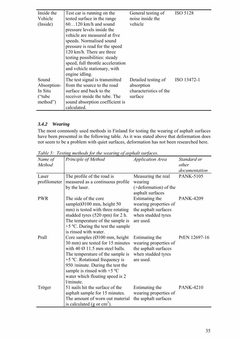
35

Inside the Vehicle (Inside)

Test car is running on the tested surface in the range 60…120 km/h and sound pressure levels inside the vehicle are measured at five speeds. Normalised sound pressure is read for the speed 120 km/h. There are three testing possibilities: steady speed, full throttle acceleration and vehicle stationary, with engine idling.

General testing of noise inside the vehicle

ISO 5128

Sound Absorption-In Situ (“tube method”)

The test signal is transmitted from the source to the road surface and back to the receiver inside the tube. The sound absorption coefficient is calculated.

Detailed testing of absorption characteristics of the surface

ISO 13472-1

3.4.2 Wearing The most commonly used methods in Finland for testing the wearing of asphalt surfaces have been presented in the following table. As it was stated above that deformation does not seem to be a problem with quiet surfaces, deformation has not been researched here. Table 5: Testing methods for the wearing of asphalt surfaces. Name of Method

Principle of Method Application Area Standard or other documentation

Laser profilometer

The profile of the road is measured as a continuous profile by the laser.

Measuring the real wearing (+deformation) of the asphalt surfaces

PANK-5105

PWR The side of the core sample(Ø100 mm, height 50 mm) is tested with three rotating studded tyres (520 rpm) for 2 h. The temperature of the sample is +5 ºC. During the test the sample is rinsed with water.

Estimating the wearing properties of the asphalt surfaces when studded tyres are used.

PANK-4209

Prall Core samples (Ø100 mm, height 30 mm) are tested for 15 minutes with 40 Ø 11.5 mm steel balls. The temperature of the sample is +5 ºC. Rotational frequency is 950 /minute. During the test the sample is rinsed with +5 ºC water which floating speed is 2 l/minute.

Estimating the wearing properties of the asphalt surfaces when studded tyres are used.

PrEN 12697-16

Tröger 51 nails hit the surface of the asphalt sample for 15 minutes. The amount of worn out material is calculated (g or cm3).

Estimating the wearing properties of the asphalt surfaces

PANK-4210

36

3.4.3 Temperature correction of the noise results To be able to repeat and reproduce the noise measurements they should be all done at the same temperature or some kind of a temperature correction should be used. A common estimate for the effect of the temperature is that a 10 °C difference in temperature means about 1 dB difference in the noise. At the moment there is no common standard for the temperature correction. The International Organisation for Standardisation (ISO) has a working group (ISO/TC 43/SC 1/WG 27) dealing with the problem but its work has not been finished yet. The tyre/road noise is known to be affected by temperature during both generation and propagation. The generation mechanisms which are most affected by the temperature can be generalised into two groups. The first involves the tread vibrational inputs which are dependent on the tread compound. The second concerns the vibrational transfer characteristics from the tread to the side wall. The influence on the overall noise level is dependent on the tyre and surface characteristics. Therefore it is likely that the influence of temperature will be different for each road surface type, although the differences are unlikely to be large in most cases. Another factor to consider is the temperature gradient existing above a road surface. During hot sunny conditions the temperature of the road surface can be very high. This produces a very hot layer of air close to the surface and a steep temperature gradient with height above the surface. Since the speed of sound is dependent on the temperature of the air, a steep temperature gradient above a road surface will tend to produce significant changes in the speed of sound with height-the speed decreasing as the temperature reduces. Under such conditions, sound waves propagating over a hot surface will be diffracted upwards by the temperature gradient. This can often lead to reduced noise levels at roadside receiver positions. [Phillips, S. et al. (1998)] The temperature correction could be done on the basis of different factors but the most commonly used are:

• tyre temperature • road surface temperature • air temperature.

The relation between the temperature and noise has been studied. It seems that the relation is between noise and road temperature or noise and air temperature. The relation between noise and tyre temperature is generally not as good. It means that one should select either road or air temperature. The choice between these two can be purely practical. The correction coefficient is anyway higher for air temperature than for road temperature. The latter is about 65 % of the former. This is because the air temperature does not vary over such a wide range as the road temperature. [Sandberg, U. et al. (2002)] Several factors seem to affect on the temperature effect. The effect of speed on the noise-temperature slope is inconsistent. Some studies suggest a higher slope at higher speeds, some suggest the contrary. Possibly there are some conflicting effect here. There is a rather big range of slopes for car tyres from +0.03 to –0.20 dB(A)/°C. The average lies between –0.03 and –0.09 for car tyres. One can see no clear pattern with regard to which tyre type may have lower or higher slopes. There is also a considerable range of slopes for road surfaces. When testing with a wide range of tyre of cars, the average is probably around –0.06 to –0.09 dB(A)/°C. However it seems that SPB-method gives somewhat lower temperature coefficients than measurements on a test track. One reason could be the age and wear of tyres. On the road, many tyres have a lower tread depth than new tyres have and tyres are generally older and stiffer than those generally used on the test tracks. [Sandberg, U. et al. (2002)]

37

The ISO standard of SPB-method and draft standard of the CPX-method give no formula for the temperature corrections. It was suggested in these papers that temperature correction should be used. Only in one draft standard for Coast-by-method, Draft International Standard (ISO/DIS 13325), a following method was introduced. (6) ( ) ( ) ( )Θ−Θ+Θ=Θ refmref KLL [dB] Where

L is corrected sound level Lm is measured sound level (dB) θ is the measured road temperature (ºC) θ ref is 20 ºC K is the temperature coefficient

For class C1 tyres (passenger car tyres)

K is -0.03 dB/ ºC if θ>θref K is -0.06 dB/ºC if θ<θref

For class C2 tyres (light truck and van tyres) K is -0.02 dB/ºC

For class C3 tyres (heavy truck tyres) K is 0

Measurements shall not be made if either the air or the test surface temperatures are below 5 ºC or the air temperature is above 40 ºC. There are also other temperature compensations and two of them have been presented in the following paper. [Lahtinen, I. et al. (1999)] In the first method, the compensation was done on the basis of the air temperature. (7) TKLL m ∆+= [dB] Where

L is the corrected sound level Lm is the measured sound level (dB) K is the temperature constant 0.08 dB/ºC

∆T is the difference between the air temperature at the time of the sound recording and the reference air temperature (20ºC)

Measurements shall not be made if either the air or test surface temperatures are below 5 ºC or the air temperature is above 40 ºC. In the second method, both the air and road temperatures were taken into the consideration: (8) AARrm TKTKLL ∆+∆+= [dB] Where

L is the corrected sound level Lm is the measured sound level (dB)

KR is the road temperature constant 0.040 dB/ºC ∆TR is the difference between the road temperature at the time of the

sound recording and the reference road temperature (20ºC) K is the air temperature constant 0.060 dB/ºC ∆TA is the difference between the air temperature at the time of the

sound recording and the reference air temperature (20ºC).

38

4 Choosing the measuring methods

4.1 Noise measurement methods

4.1.1 General Possible noise measurement methods were considered carefully and some of them were evaluated. Test method will be used for surfaces outdoors when also the laying work pays an important role. That is why the laboratory drum-method was left out. Tube-method was interesting and some basic calculations were made for building the device for this method. It was decided that further information about this method in road noise measurements from other countries is needed before testing this method in Finland. CB– and INSIDE-methods were both seen to be simple and easy methods to run and they were tested in the HILJA-project. INSIDE- and CB-methods have some disadvantages when used for quality controlling. The results of these methods are highly dependent on the vehicle and tyres used in the measurements. The same problem is with the Controlled pass-by method. Two methods, SBP and CPX, were chosen for further investigation. SPB- and CPX-methods have both been used for surface testing in the other countries as well. These two methods were chosen for further testing so that it would be possible to see how these methods work in Finland.

4.1.2 Statistical Pass-by (ISO 11819-1) In the Statistical Pass-by (SPB) method, the maximum A-weighted sound pressure levels, LAmax, (using time weighting “fast”) of individual vehicle pass-bys are measured together with the vehicle speeds. Each measured vehicle is classified into one of three vehicle categories: “cars”, “dual-axle heavy vehicles“ and “multi-axle heavy vehicles”. Three categories of roads are defined with respect to the range of speeds at which the traffic flows. There is a nominated reference speed given to each speed category. Speed categories and reference speeds are: • “low “ road speed category (45-64 km/h); reference speed 50 km/h • “medium” road speed category (65-99 km/h); reference speed 80 km/h • “high” road speed category (100 km/h or more); reference speed 110 km/h. Test sites should meet the following criteria: • Each test section shall extend at least 30 m on both sides from the microphone

location. For “high” road speed category the distance is increased to 50 m. • The road shall be essentially level and straight. Roads with slight bends or with

gradient ≤ 1% may be considered as valid test sites. • The number of vehicles judged to be moving at constant speed shall be sufficient in

order to allow a reasonable total measuring time. • Just prior to and just after the passage of a vehicle intended for measurement, the A-

weighted sound pressure level shall be at least 6 dB below the measured maximum A-weighted sound pressure level under the pass-by.

• The road surface shall be in a good condition, unless the intention is to study the effect of condition.

• The traffic flowing on the road section should contain sufficient numbers of each category of vehicle to enable a full analysis.

39

For surface classification purposes, the measurement microphone should be located in the acoustical free field (Fig. 14, 15). This means that acoustic reflections from surfaces such as building facades, noise barriers, road cuttings and embankments shall be at least 10 dB lower than the direct sound to be measured. As a guideline, 25 m of space around the microphone free of any reflecting objects other than the ground is usually adequate to ensure that approximate free field conditions exist.

Central line Test lane

Microphone

7,5 m

10 m

10 m10 m

10 m

10 m10 m

No reflecting objects inside this area

Figure 14: Requirements regarding freedom from reflecting or screening safety barriers or guard rails.

Test lane

Microphone

7,5 m

20 m20 m

>5 m >3,75

Material having the same sound absorption than the tested surface

Area with arbitary covering; no tall plants

No requirements

Center of test lane

Figure 15: Requirements regarding the minimum coverage with acoustically

appropriate surface between the test lane and the microphone. The horizontal distance from the microphone position to the centre of the lane in which the vehicles to be measured travel shall be 7.5 m ±0.1 m. The microphone shall be located 1.2 m ± 0.1 m above the plane of the road lane (Fig. 16).

40

Figure 16: Test setting of the SPBmod-method [Sainio, P. (2000)] The following minimum numbers of vehicles shall be measured, within each category: • cars min. 100 • dual-axle heavy vehicles min. 30 • multi-axle heavy vehicles min. 30 • dual- and multi-axle heavy vehicles together min. 80 Only vehicles which clearly fall within any of the vehicle categories shall be measured. Measurements shall only be taken on individual vehicle pass-bys which can be clearly distinguished acoustically from other traffic on the road. During the measurements wind speed at the microphone height shall not exceed 5 m/s. Air temperature shall be within 5 °C to 30 °C. The road surface temperature shall be within 5 °C to 50 °C. The Vehicle Sound Levels should be corrected to a reference air temperature of 20 °C. A suitable method is at present under consideration. A linear regression analysis of sound pressure levels on speed shall be made using data pairs consisting of the maximum A-weighted sound levels versus logarithm of speed for each vehicle pass-by. A regression line shall be fit to the data points for each separate vehicle category, using the least squares method. The reference speeds for the vehicle categories in the road speed categories are specified in table 6 below. The ordinate sound level of the regression line for each category of vehicle at the corresponding reference speed is taken to be the Vehicle Sound Level Lveh. In this way, for certain road sites, three Lveh values are obtained: for cars, dual-axle heavy vehicles and multi-axle heavy vehicles. Table 6: Reference speeds and weighting factors (Wx) in the different road speed

categories. [ISO 11819-1] Road speed category Vehicle category

Low Medium High Name No. Ref. speed

(km/h) Wx Ref. speed

(km/h) Wx Ref. speed

(km/h) Wx

Cars 1 50 0.900 80 0.800 110 0.700Dual-axle heavy vehicles

2a 50 0.075 70 0.100 85 0.075

Multi-axle heavy vehicles

2b 50 0.025 70 0.100 85 0.225

41

For the regression calculation and subsequent normalisation to a reference speed the following condition shall be met. The range of speeds covered by the measured vehicles shall be such that the reference speed shall be within the range of plus-or-minus one standard deviation from the actually measured average speed for heavy vehicles and plus-or-minus one-and-a-half standard deviation for cars. In order to obtain an average level of road surface influence on traffic noise for a mix of vehicles, a Statistical Pass-By Index shall be calculated as follows:

(9) ⎥⎦

⎤⎢⎣

⎡×⎟⎟⎠

⎞⎜⎜⎝

⎛×+×⎟⎟

⎠

⎞⎜⎜⎝

⎛×+××= 10

2

12

10

2

12

101

221

101010lg10ba L

bb

L

aa

L

vvW

vvWWSPBI [dB]

Where SPBI is the Statistical Pass-by Index, for standard mix of light and

heavy vehicles L1, L2, L3 are the Vehicle Sound Levels for vehicle categories 1, 2a and 2b (dB) W1,W2, W3 are the weighting factors, which are equivalent to the assumed

proportions of vehicle categories in the traffic, according to the table 6.

v1,v2a, v2b are the reference speeds of individual vehicle categories, according to table 6 (km/h).

Typical values for the weighting factors W1,W2, W3 may vary considerably from place to place, country to country and with time of day and night. The values selected to table 6 should represent globally most typical cases which allow simple comparison of road surfaces. In Finland the devices and computer programs for the SPBmod-measurements were built in the Laboratory of Automotive Engineering (HUT).This system was used in this research as well. Devices are (Fig. 17 ):

• Ono Sokki-sound level meter • VAISALA-weather station • two laser ports for measuring speed • portable computer with HUT SPB-measuring program.

LAmax decibel values are measured together with the speed and meteorological information (road and air temperature, together with the wind speed).

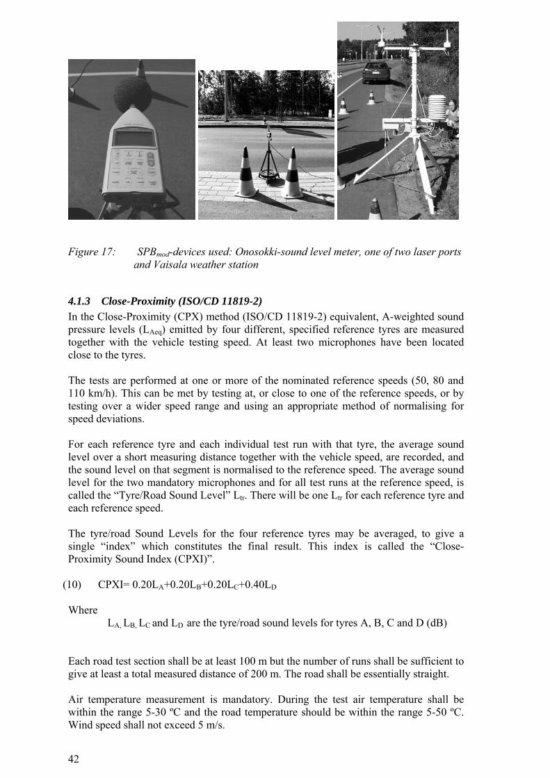
42

Figure 17: SPBmod-devices used: Onosokki-sound level meter, one of two laser ports

and Vaisala weather station

4.1.3 Close-Proximity (ISO/CD 11819-2) In the Close-Proximity (CPX) method (ISO/CD 11819-2) equivalent, A-weighted sound pressure levels (LAeq) emitted by four different, specified reference tyres are measured together with the vehicle testing speed. At least two microphones have been located close to the tyres. The tests are performed at one or more of the nominated reference speeds (50, 80 and 110 km/h). This can be met by testing at, or close to one of the reference speeds, or by testing over a wider speed range and using an appropriate method of normalising for speed deviations. For each reference tyre and each individual test run with that tyre, the average sound level over a short measuring distance together with the vehicle speed, are recorded, and the sound level on that segment is normalised to the reference speed. The average sound level for the two mandatory microphones and for all test runs at the reference speed, is called the “Tyre/Road Sound Level” Ltr. There will be one Ltr for each reference tyre and each reference speed. The tyre/road Sound Levels for the four reference tyres may be averaged, to give a single “index” which constitutes the final result. This index is called the “Close-Proximity Sound Index (CPXI)”.

(10) CPXI= 0.20LA+0.20LB+0.20LC+0.40LD Where

LA, LB, LC and LD are the tyre/road sound levels for tyres A, B, C and D (dB)

Each road test section shall be at least 100 m but the number of runs shall be sufficient to give at least a total measured distance of 200 m. The road shall be essentially straight. Air temperature measurement is mandatory. During the test air temperature shall be within the range 5-30 ºC and the road temperature should be within the range 5-50 ºC. Wind speed shall not exceed 5 m/s.

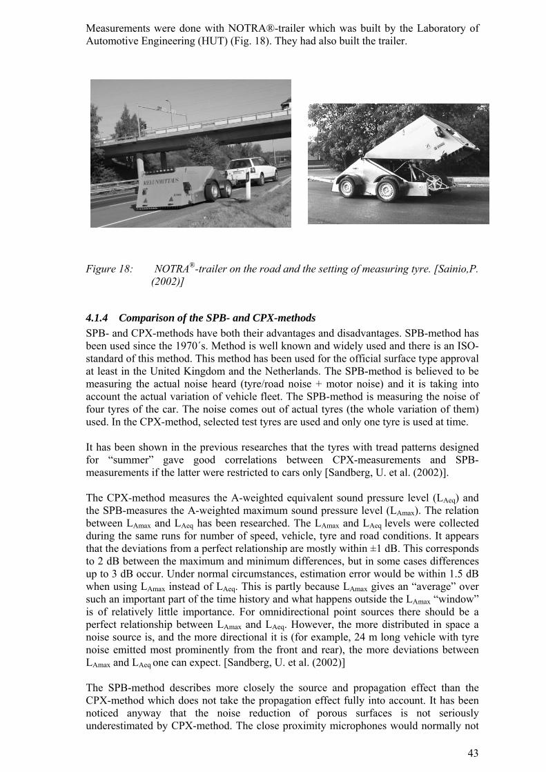
43

Measurements were done with NOTRA®-trailer which was built by the Laboratory of Automotive Engineering (HUT) (Fig. 18). They had also built the trailer. Figure 18: NOTRA®-trailer on the road and the setting of measuring tyre. [Sainio,P.

(2002)]

4.1.4 Comparison of the SPB- and CPX-methods SPB- and CPX-methods have both their advantages and disadvantages. SPB-method has been used since the 1970´s. Method is well known and widely used and there is an ISO-standard of this method. This method has been used for the official surface type approval at least in the United Kingdom and the Netherlands. The SPB-method is believed to be measuring the actual noise heard (tyre/road noise + motor noise) and it is taking into account the actual variation of vehicle fleet. The SPB-method is measuring the noise of four tyres of the car. The noise comes out of actual tyres (the whole variation of them) used. In the CPX-method, selected test tyres are used and only one tyre is used at time. It has been shown in the previous researches that the tyres with tread patterns designed for “summer” gave good correlations between CPX-measurements and SPB-measurements if the latter were restricted to cars only [Sandberg, U. et al. (2002)]. The CPX-method measures the A-weighted equivalent sound pressure level (LAeq) and the SPB-measures the A-weighted maximum sound pressure level (LAmax). The relation between LAmax and LAeq has been researched. The LAmax and LAeq levels were collected during the same runs for number of speed, vehicle, tyre and road conditions. It appears that the deviations from a perfect relationship are mostly within ±1 dB. This corresponds to 2 dB between the maximum and minimum differences, but in some cases differences up to 3 dB occur. Under normal circumstances, estimation error would be within 1.5 dB when using LAmax instead of LAeq. This is partly because LAmax gives an “average” over such an important part of the time history and what happens outside the LAmax “window” is of relatively little importance. For omnidirectional point sources there should be a perfect relationship between LAmax and LAeq. However, the more distributed in space a noise source is, and the more directional it is (for example, 24 m long vehicle with tyre noise emitted most prominently from the front and rear), the more deviations between LAmax and LAeq one can expect. [Sandberg, U. et al. (2002)] The SPB-method describes more closely the source and propagation effect than the CPX-method which does not take the propagation effect fully into account. It has been noticed anyway that the noise reduction of porous surfaces is not seriously underestimated by CPX-method. The close proximity microphones would normally not

44

be expected to take the sound propagation effect of porous surfaces fully into account. However, something seems to compensate for this. [Sandberg, U. et al. (2002)] The limitation of the SPB-measurements is that they are done only in one spot when the CPX-results are representing a longer stretch of the road. CPX-method can be used for the homogeneity check of the road. The correlation between roadside and close proximity measurements has been researched. By averaging the overall A-weighted noise levels obtained at the two microphone positions specified in the ISO-standard, values of close proximity noise levels have been correlated with maximum coast-by noise levels obtained on the same road surfaces. A regression analysis was then used to determine the functional relationship between these two variables and this relationship took the form of:

(11) 082,142

9939,0 21)max( −⎟

⎠⎞

⎜⎝⎛ +

×=SPLMSPLML cA [dB] R2=0,85

Where

LAmax (c) is the calculated overall coast –by noise level SPLMn is the overall close proximity sound pressure level at

microphone n (dB)

[Phillips, S. (2002)] The results of comparing the coast-by levels measured on a variety of surface types and the corresponding CPX-levels obtained from the equation above showed that though there is a good agreement between the measured and predicted levels (85% of the variance in the calculated levels explained), several outliers remained. In an attempt to improve the accuracy of prediction the analysis of frequency spectra showed that significant improvements were possible by selecting the most highly correlated frequency components. It was possible to improve the variance explained to 93 %. SPB-results were not used in this research but signs are encouraging that a high degree of correspondence between CPX- and roadside noise could be obtained. [Phillips, S. (2001)]

4.1.5 Modification of SPB- and CPX-methods In this study SPB-, CPX-methods were not done by the standards. From now on in this paper the modified methods used will be called SPBmod and CPXmod. The reasons of modifications are explained below. When measuring with the SPB-method it was soon noticed that there is not enough heavy traffic to fulfil the demand of 80 heavy vehicles per measurement. The heavy vehicles were measured anyway for a pure interest and the average number of heavy vehicles per hour was following: Table 7: The average number of heavy vehicles per hour. Test Road Average number of

heavy vehicles/hour Kaarina 8 Kokkola 8 Helsinki 7 Kirkkonummi 14 Espoo 3 Lohja 7

45

Including the heavy vehicles would have meant a huge increase in the measurement time. The number of heavy vehicles on some test roads was so low that it was not possible to do any statistical evaluation of their noise emissions. It was decided that heavy vehicles will be left out and SPBI will not be calculated. The results of 100 cars will be normalised and these LAmax values will be compared with each other as such. This change will make the measurement time reasonable and costs realistic. Though the heavy vehicles were left out it is still possible to compare different asphalt products with each other. SPB-standard sets three different reference speeds for normalisation: 50 km/h, 80 km/h and 110 km/h. The standard says that for the regression calculation and subsequent normalisation to a reference speed the following condition shall be met. The range of speeds covered by the measured vehicles shall be such that the reference speed shall be within the range of plus-or-minus one-and-a-half standard deviation for cars. To fulfil this criterion it was impossible to use the normalisation speeds suggested by the standard. In the areas where the speed limit was 50 km/h the cars were driving a little faster. Results measured would not have fulfilled the criteria set by the standard if the normalisation speed was 50 km/h. In the highest category it was chosen to use the 100 km/h as a reference speed because it was the actual speed limit. It was chosen that the normalisation speeds in Finland are 60 km/h, 80 km/h and 100 km/h. Because of modifications the results measured with the SPBmod-method can not be compared with the SPBI-results measured in the other countries. Anyhow they can be compared with the results of the category “cars” if the normalisation speed is the same. According to the Draft Standard of CPX-method four different tyres shall be used. All these tyres were not available when the research started, so it was decided to use only the ASTM E 524 (slick) for the measurements. This same method had been used earlier in Finland when the Laboratory of Automotive Engineering (HUT) developed their NOTRA-trailer and used it for some measures. It was seen as an advantage to keep this method same so that results could be compared. The Laboratory of Automotive Engineering had decided to use the ASTM E524 smooth tyre in order to avoid possibilities of tread pattern different operation on different surfaces. The second argument was that there would be similar reference tyres available over longer time period than normal production age with out the danger of modifications of normal production tyre model. [Sainio, P. (2003)] The tyre pressure was 1.9 bars and the static load of the test tyre was 3900N. This tyre is commercially available also in future. The measurement speed was 50 km/h. LAeq decibel-values were measured together with the speed and air temperature. Frequency spectrums were also measured. CPXI was not calculated but surfaces were compared by comparing the measured LAeq. Because of these changes the results measured with the CPXmod-method can not be compared with the CPXI-results measured in the other countries.

4.2 Wearing measurement methods

4.2.1 General PWR- and Prall-tests have replaced Tröger in surface testing. Nowadays commonly used methods for predicting the wearing of surfaces are Prall- and PWR-tests. In general there

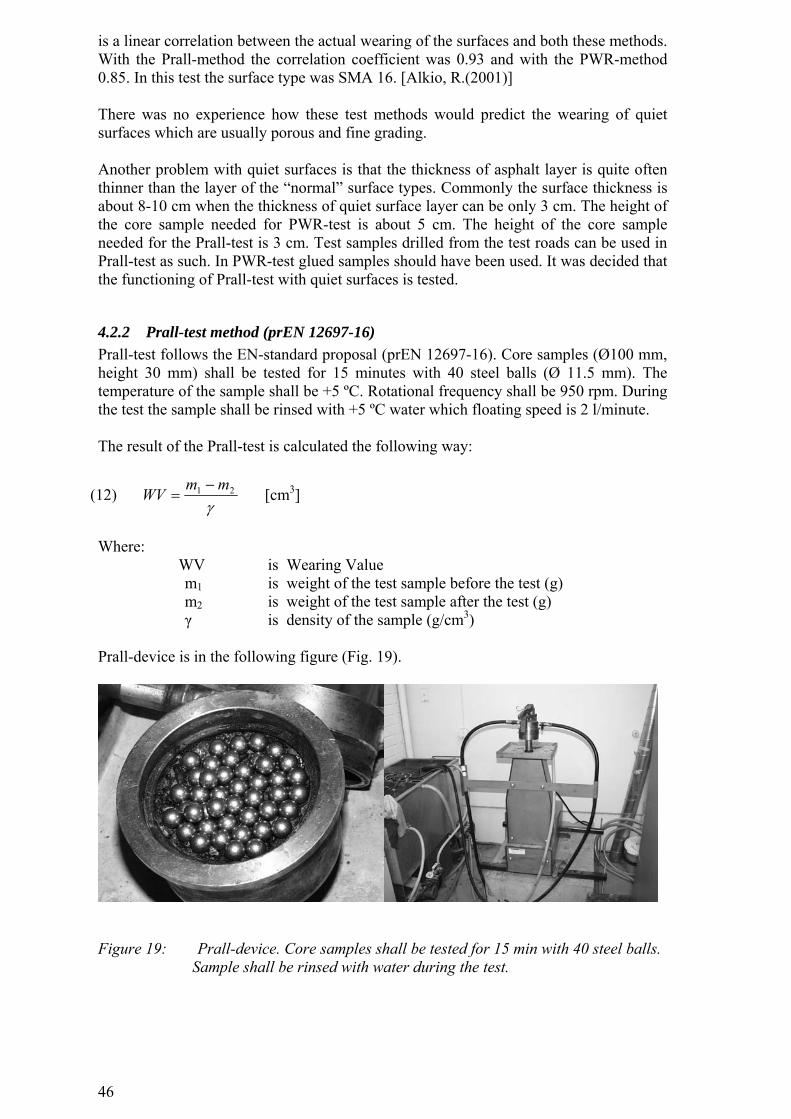
46

is a linear correlation between the actual wearing of the surfaces and both these methods. With the Prall-method the correlation coefficient was 0.93 and with the PWR-method 0.85. In this test the surface type was SMA 16. [Alkio, R.(2001)] There was no experience how these test methods would predict the wearing of quiet surfaces which are usually porous and fine grading. Another problem with quiet surfaces is that the thickness of asphalt layer is quite often thinner than the layer of the “normal” surface types. Commonly the surface thickness is about 8-10 cm when the thickness of quiet surface layer can be only 3 cm. The height of the core sample needed for PWR-test is about 5 cm. The height of the core sample needed for the Prall-test is 3 cm. Test samples drilled from the test roads can be used in Prall-test as such. In PWR-test glued samples should have been used. It was decided that the functioning of Prall-test with quiet surfaces is tested.

4.2.2 Prall-test method (prEN 12697-16) Prall-test follows the EN-standard proposal (prEN 12697-16). Core samples (Ø100 mm, height 30 mm) shall be tested for 15 minutes with 40 steel balls (Ø 11.5 mm). The temperature of the sample shall be +5 ºC. Rotational frequency shall be 950 rpm. During the test the sample shall be rinsed with +5 ºC water which floating speed is 2 l/minute. The result of the Prall-test is calculated the following way:

(12) γ

21 mmWV −= [cm3]

Where:

WV is Wearing Value m1 is weight of the test sample before the test (g) m2 is weight of the test sample after the test (g) γ is density of the sample (g/cm3)

Prall-device is in the following figure (Fig. 19).

Figure 19: Prall-device. Core samples shall be tested for 15 min with 40 steel balls.

Sample shall be rinsed with water during the test.

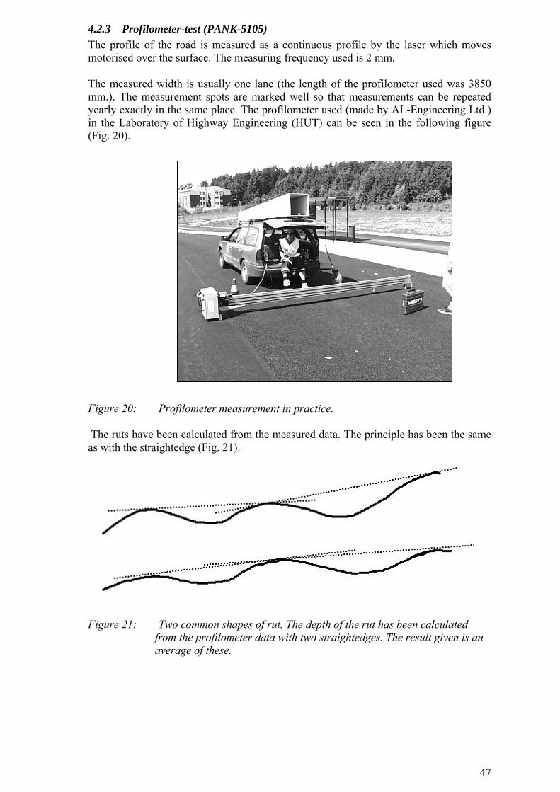
47

4.2.3 Profilometer-test (PANK-5105) The profile of the road is measured as a continuous profile by the laser which moves motorised over the surface. The measuring frequency used is 2 mm. The measured width is usually one lane (the length of the profilometer used was 3850 mm.). The measurement spots are marked well so that measurements can be repeated yearly exactly in the same place. The profilometer used (made by AL-Engineering Ltd.) in the Laboratory of Highway Engineering (HUT) can be seen in the following figure (Fig. 20). Figure 20: Profilometer measurement in practice. The ruts have been calculated from the measured data. The principle has been the same as with the straightedge (Fig. 21).

Figure 21: Two common shapes of rut. The depth of the rut has been calculated

from the profilometer data with two straightedges. The result given is an average of these.

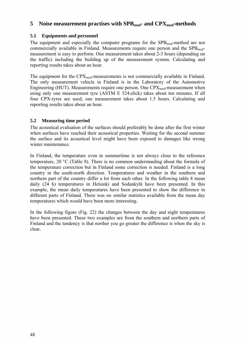
48

5 Noise measurement practises with SPBmod- and CPXmod-methods

5.1 Equipments and personnel The equipment and especially the computer programs for the SPBmod-method are not commercially available in Finland. Measurements require one person and the SPBmod-measurement is easy to perform. One measurement takes about 2-3 hours (depending on the traffic) including the building up of the measurement system. Calculating and reporting results takes about an hour. The equipment for the CPXmod-measurements is not commercially available in Finland. The only measurement vehicle in Finland is in the Laboratory of the Automotive Engineering (HUT). Measurements require one person. One CPXmod-measurement when using only one measurement tyre (ASTM E 524;slick) takes about ten minutes. If all four CPX-tyres are used, one measurement takes about 1.5 hours. Calculating and reporting results takes about an hour.

5.2 Measuring time period The acoustical evaluation of the surfaces should preferably be done after the first winter when surfaces have reached their acoustical properties. Waiting for the second summer the surface and its acoustical level might have been exposed to damages like wrong winter maintenance. In Finland, the temperature even in summertime is not always close to the reference temperature, 20 °C (Table 8). There is no common understanding about the formula of the temperature correction but in Finland some correction is needed. Finland is a long country in the south-north direction. Temperatures and weather in the southern and northern part of the country differ a lot from each other. In the following table 8 mean daily (24 h) temperatures in Helsinki and Sodankylä have been presented. In this example, the mean daily temperatures have been presented to show the difference in different parts of Finland. There was no similar statistics available from the mean day temperatures which would have been more interesting. In the following figure (Fig. 22) the changes between the day and night temperatures have been presented. These two examples are from the southern and northern parts of Finland and the tendency is that norther you go greater the difference is when the sky is clear.

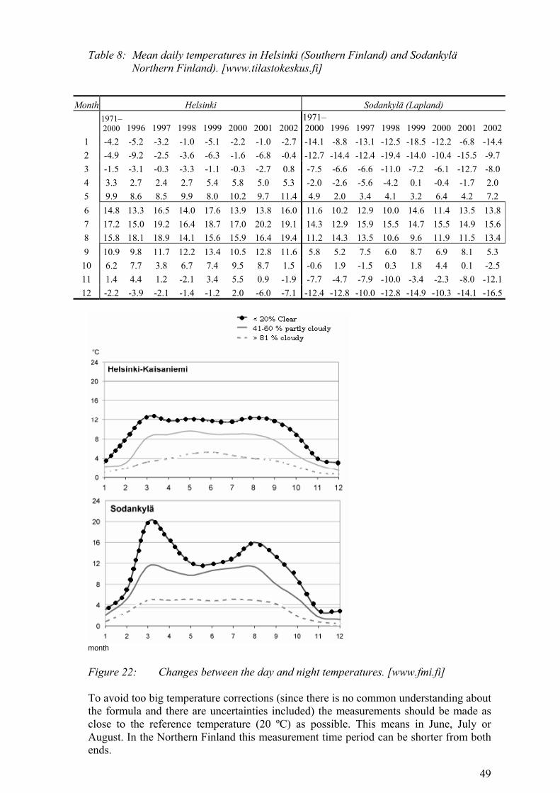
49

Table 8: Mean daily temperatures in Helsinki (Southern Finland) and Sodankylä

Northern Finland). [www.tilastokeskus.fi]

month Figure 22: Changes between the day and night temperatures. [www.fmi.fi] To avoid too big temperature corrections (since there is no common understanding about the formula and there are uncertainties included) the measurements should be made as close to the reference temperature (20 ºC) as possible. This means in June, July or August. In the Northern Finland this measurement time period can be shorter from both ends.

Month Helsinki Sodankylä (Lapland)

1971–2000 1996 1997 1998 1999 2000 2001 2002

1971–2000 1996 1997 1998 1999 2000 2001 2002

1 -4.2 -5.2 -3.2 -1.0 -5.1 -2.2 -1.0 -2.7 -14.1 -8.8 -13.1 -12.5 -18.5 -12.2 -6.8 -14.42 -4.9 -9.2 -2.5 -3.6 -6.3 -1.6 -6.8 -0.4 -12.7 -14.4 -12.4 -19.4 -14.0 -10.4 -15.5 -9.7 3 -1.5 -3.1 -0.3 -3.3 -1.1 -0.3 -2.7 0.8 -7.5 -6.6 -6.6 -11.0 -7.2 -6.1 -12.7 -8.0 4 3.3 2.7 2.4 2.7 5.4 5.8 5.0 5.3 -2.0 -2.6 -5.6 -4.2 0.1 -0.4 -1.7 2.0 5 9.9 8.6 8.5 9.9 8.0 10.2 9.7 11.4 4.9 2.0 3.4 4.1 3.2 6.4 4.2 7.2 6 14.8 13.3 16.5 14.0 17.6 13.9 13.8 16.0 11.6 10.2 12.9 10.0 14.6 11.4 13.5 13.87 17.2 15.0 19.2 16.4 18.7 17.0 20.2 19.1 14.3 12.9 15.9 15.5 14.7 15.5 14.9 15.68 15.8 18.1 18.9 14.1 15.6 15.9 16.4 19.4 11.2 14.3 13.5 10.6 9.6 11.9 11.5 13.49 10.9 9.8 11.7 12.2 13.4 10.5 12.8 11.6 5.8 5.2 7.5 6.0 8.7 6.9 8.1 5.3

10 6.2 7.7 3.8 6.7 7.4 9.5 8.7 1.5 -0.6 1.9 -1.5 0.3 1.8 4.4 0.1 -2.5 11 1.4 4.4 1.2 -2.1 3.4 5.5 0.9 -1.9 -7.7 -4.7 -7.9 -10.0 -3.4 -2.3 -8.0 -12.112 -2.2 -3.9 -2.1 -1.4 -1.2 2.0 -6.0 -7.1 -12.4 -12.8 -10.0 -12.8 -14.9 -10.3 -14.1 -16.5

50

The Laboratory of Automotive Engineering (HUT) measured certain test roads in the Southern Finland during several years once a month. [Sainio, P. (2003)] All the measurements were done inside the temperature limits (5-30 ºC) given by the draft ISO- standard. Results were temperature corrected by the air temperature (Formula 7). In these CPXmod-results it can be seen that there are monthly changes in the results (Fig. 23). Difference between different months is over 3 dB in the “worst” case (Korso; 05/2001…09/2001) and in the most cases the difference is over 1 dB which is the repeatability of the method. There is no clear pattern and there are not enough results to make clear statements but it seems that in most cases the results from the spring are bigger than results from the autumn. One reason could be that studded tyres are commonly used until the mid April. After that the rough surfaces will smoothen a little during the summer. It was also found out that the major difference between the seasons is located at the low frequencies under 500 Hz. [Sainio, P. (2003)] Figure 23: Monthly CPXmod-results (LAeq) on MOBILE test roads [Sainio, P. (2003)] During three summer months (June, July and August) the average difference between the largest and smallest values measured was 0.56 dB when the maximum difference was 0.8 dB and minimum 0.2 dB. This difference is already inside the measurement repeatability. All the CPXmod-measurements have been taken within the temperature limits set in the draft ISO-standard of CPX. It seems that in Finland that is not enough. Temperature limits would allow us to measure about from April to October. The “measurement window” in Finland and other countries with similar conditions is more limited than that suggested in the standards (5-30 ºC).

5.3 Weather conditions during the measurements The test surface should be dry during the measurement. Different types of surfaces behave differently in wet conditions and dry differently after the rain (Fig. 24). The noise level of porous asphalt increases by about 3.5 dB with a similar increase of about 3.2 dB for SMA surface compared with the measured levels when dry. After the rain

Evolution of noise in tyre-road interaction:CPX ( 50 km/h)

93,1

90,1

90,1

90,1

93,2

93,0

90,3

88,2

88,3

93,2

92,2

90,1

88,5 88

,7

92,792

,9

89,9

87,9

88,4

92,8

92,2

89,5

86,8 87

,2

92,1

91,7

88,6

87,5 87

,8

92,0

92,6

89,7 89

,8

89,8

92,4

92,1

90,5

89,1

89,6

92,692

,9

89,9

89,9

89,2

92,5

93,7

90,7

89,3

89,3

92,8

92,9

90,0

89,1 89

,4

92,893,0

89,8

89,2

89,1

92,9

91,8

89,3

87,7

88,7

92,9

89,1

88,2

89,4

92,1

92,1

89,5

89,0 89

,2

92,7

92,3

86

88

90

92

94

96

Kehä I Vallikal-Porint 50km/h Röylä 50km/h Korso 50km/h Jokimäki 50km/h Kehä III SMA18 50km/h

05/2001

06/2001

07/2001

08/2001

09/2001

10/2001

4/2002

5/2002

6/2002

7/2002

8/2002

9/2002

4/2003

5/2003

6/2003

51

stopped, the increase in noise appeared to decay exponentially with time. Figure 24 shows the average increase in noise (above that measured when dry) for each hour over a 12-hour period after the rain stopped. For the HRA surface, similarly monitored for comparison, noise levels after the rain had stopped were not significantly different from those measured under dry conditions. [Phillips, S. et al. (2001)] Figure 24: Increase in traffic noise for different surfaces after rainfall. [Phillips, S.

et al. (2001)] The suggestion is that 24 hours should be waited after the rain before the noise measurements. If the surface is porous 36 hours should be waited.

52

6 Test Roads and Sections

6.1 General The test roads were built in different parts of Finland (Fig. 25). Three of these roads were built in 2001 and three in 2002. Suitable roads were selected from the yearly surfacing programs of the Finnish Road Administration and municipals. They were roads which would have been paved that year anyway. It was not easy to find suitable roads for this research. A test road had to be long enough, each tested product should have had as equal site as possible and the noise measurement methods set also some criteria for test roads. The maximum number of 12 products were tested in some test roads. Some surfaces outside these test roads were also measured as references. At this stage of the research, all the surfaces laid are called either quiet or reference surfaces. The real quietness of the tested quiet surfaces was evaluated later.

Figure 25: Location of test roads.

6.2 Test roads built in 2001

6.2.1 Northern Bypass, Kokkola The Northern bypass of Kokkola (road number 749) has one carriageway and two lanes (Fig.26). The speed limit is 60 km/h. The test section was perfect for noise measurements: road was straight, no traffic lights and there were no noise reflecting objects nearby. Test surfaces were laid between the 1st and 3rd of August, 2001. There are two quiet surface sections which were normal SMA-surfaces made with the remix-technique and one reference section, SMA 18 (Table 9). Valtatie laid all the surfaces. Each test section is about 500 m long and the test surfaces cover both lanes. Table 9: Tested products in Kokkola Section Contractor Product 1 Valtatie SMA 8 2 Valtatie SMA 5 3 Valtatie SMA 18 Traffic volume was calculated in November 2001 by Laboratory of Highway Engineering (HUT). The results were following:

Lohja

Espoo and Helsinki

Kokkola

Kaarina

Kirkkomummi

53

Table 10: Traffic volumes in Kokkola Section Light vehicles Heavy vehicles 1, 2& 3 from south 1891 153 1, 2& 3 from north 1779 139

Figure 26: Kokkola test road

6.2.2 Kaarinantie, Kaarina Kaarinantie (road number 2200) has one carriageway and two lanes. The speed limit is 60 km/h. The test road has some up and down hills, some intersections without traffic lights and some curves (Fig. 27). Test surfaces were laid between the 12th and 18th of September, 2001. There are four quiet surface test sections and one reference section, SMA 16 (Table 11). The Finnish Road Enterprise laid all the other surfaces expect Novachip. Lemminkäinen used their own special equipment for this surface. Each test section is 200 m long and test surface cover both lanes. Table 11: Tested products in Kaarina Section Contractor Product 1 (ref) The Finnish Road Enterprise SMA 16 2 The Finnish Road Enterprise SMA 6 3 The Finnish Road Enterprise SMA 6 4 Lemminkäinen Whisperphalt 5 Lemminkäinen Novachip Traffic volume was calculated in April, 2002 by Laboratory of Highway Engineering (HUT). The results were following:

1 3

railway Jänismaa

North

2

54

Table 12: Traffic volumes in Kaarina Section Light vehicles Heavy vehicles 3,4&5 from south 4336 443 3,4&5 from north 4271 423 1&2 from south 4355 440 1& 2 from north 4265 421

Figure 27: Kaarina test road in winter

6.2.3 Meripellontie, Helsinki Meripellontie (Fig. 28) runs between Itäkeskus and Vuosaari in Helsinki. It has two carriageways and four lanes. From the direction of Itäkeskus the speed limit is 50 km/h but it changes to 60 km/h in the middle of the test road. There are two traffic-light-guided intersections which prevent the vehicles from moving freely. Curbs line both sides of the carriageways. Test surfaces were laid between the 14th of June and the 7th of July, 2001. There are 11 quiet surface sections and one reference section, SMA 16 (Table 13). Sections 1-6 have two layers. Their thickness is about 60+30 mm. Each section is 200 m. Carriageways were drained. Each contractor laid their products themselves. The reference surface was laid by Valtatie.

1. 5. 4. 3.

Häm

eenvaltatie

North

2.

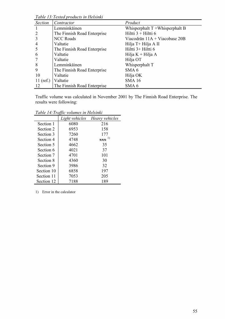
55

Table 13: Tested products in Helsinki Section Contractor Product 1 Lemminkäinen Whisperphalt T +Whisperphalt B 2 The Finnish Road Enterprise Hiltti 3 + Hiltti 6 3 NCC Roads Viacodrän 11A + Viacobase 20B 4 Valtatie Hilja T+ Hilja A II 5 The Finnish Road Enterprise Hiltti 3+ Hiltti 6 6 Valtatie Hilja K + Hilja A 7 Valtatie Hilja OT 8 Lemminkäinen Whisperphalt T 9 The Finnish Road Enterprise SMA 6 10 Valtatie Hilja OK 11 (ref.) Valtatie SMA 16 12 The Finnish Road Enterprise SMA 6 Traffic volume was calculated in November 2001 by The Finnish Road Enterprise. The results were following: Table 14: Traffic volumes in Helsinki

Light vehicles Heavy vehicles Section 1 6080 216 Section 2 6953 158 Section 3 7260 177 Section 4 4748 xxx 1) Section 5 4662 35 Section 6 4021 37 Section 7 4701 101 Section 8 4360 30 Section 9 3986 32 Section 10 6858 197 Section 11 7053 205 Section 12 7188 189 1) Error in the calculator

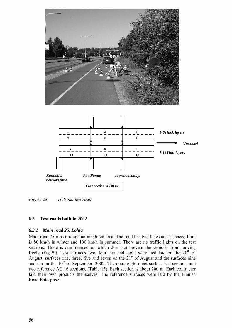
56

Figure 28: Helsinki test road

6.3 Test roads built in 2002

6.3.1 Main road 25, Lohja Main road 25 runs through an inhabited area. The road has two lanes and its speed limit is 80 km/h in winter and 100 km/h in summer. There are no traffic lights on the test sections. There is one intersection which does not prevent the vehicles from moving freely (Fig.29). Test surfaces two, four, six and eight were lied laid on the 20th of August, surfaces one, three, five and seven on the 21st of August and the surfaces nine and ten on the 10th of September, 2002. There are eight quiet surface test sections and two reference AC 16 sections. (Table 15). Each section is about 200 m. Each contractor laid their own products themselves. The reference surfaces were laid by the Finnish Road Enterprise.

1-6Thick layers

7-12Thin layers

Vuosaari

JuorumäenkujaPuotilantie Kunnallis- neuvoksentie

1 2 3

4 5 6

8 9

11 12

Each section is 200 m

7

10

57

Table 15: Tested products in Lohja Section Contractor Product 1 (ref) The Finnish Road Enterprise AC 16 2 (ref) The Finnish Road Enterprise AC 16 3 NCC Roads Viacodrän 16 4 NCC Roads Viacodrän 11 5 The Finnish Road Enterprise Hiltti A 6 The Finnish Road Enterprise Hiltti F 7 Valtatie SHP-KY4 8 Valtatie SHP-K3 9 Lemminkäinen Novachip 10 Lemminkäinen Novachip Traffic volume was calculated in December 2002 by the Finnish Road Enterprise. The results were following: Table 16: Traffic volumes in Lohja

Light vehicles Heavy vehicles Sections 1,3,5,7 and 9 3168 535 Sections 2,4,6,8 and 10 3152 464

Gunnarla

10 8 6 4 2

9 7 1 3 5 North

Figure 29: Test road in Lohja

58

6.3.2 Riihiniityntie, Espoo Riihiniityntie is a collecting street in a single-family house area in Espoo. The street has two lanes and the speed limit is 50 km/h. There are no traffic lights or major intersections which prevent the vehicles from moving freely (Fig. 30). Test surfaces were laid in the 1st of August, 2002, except the section one which was laid later on the 10th of September, 2002. There are eight quiet test sections and two reference sections, AC 16 and SMA 8 (Table 17). Each section is about 150 m (reference sections 320 m). Each contractor laid their own products themselves. The reference surfaces were laid by Lemminkäinen. Table 17: Tested products in Espoo Section Contractor Product 1 Lemminkäinen Novachip 2 Lemminkäinen Whisperphalt T 3 The Finnish Road Enterprise Hiltti-mix 4 The Finnish Road Enterprise SMA 6 5 NCC Roads Viacodrän 8 6 NCC Roads Viacodrän 11 7 Valtatie SHP-Y 8 Valtatie SHP-K2 9 (ref) Lemminkäinen SMA 8 10 (ref) Lemminkäinen AC 16 Traffic volume was calculated in March, 2003, by Laboratory of Highway Engineering (HUT). The results were following: Table 18: Traffic volumes in Espoo

Light vehicles Heavy vehicles Sections 1-4 and 9 2153 78 Sections 5-8 and 10 2175 74

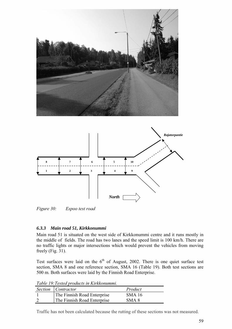
59

Rajatorpantie

8

1 2 4 9

1056 7

3

North

Figure 30: Espoo test road

6.3.3 Main road 51, Kirkkonummi Main road 51 is situated on the west side of Kirkkonummi centre and it runs mostly in the middle of fields. The road has two lanes and the speed limit is 100 km/h. There are no traffic lights or major intersections which would prevent the vehicles from moving freely (Fig. 31). Test surfaces were laid on the 6th of August, 2002. There is one quiet surface test section, SMA 8 and one reference section, SMA 16 (Table 19). Both test sections are 500 m. Both surfaces were laid by the Finnish Road Enterprise. Table 19: Tested products in Kirkkonummi. Section Contractor Product 1 The Finnish Road Enterprise SMA 16 2 The Finnish Road Enterprise SMA 8 Traffic has not been calculated because the rutting of these sections was not measured.

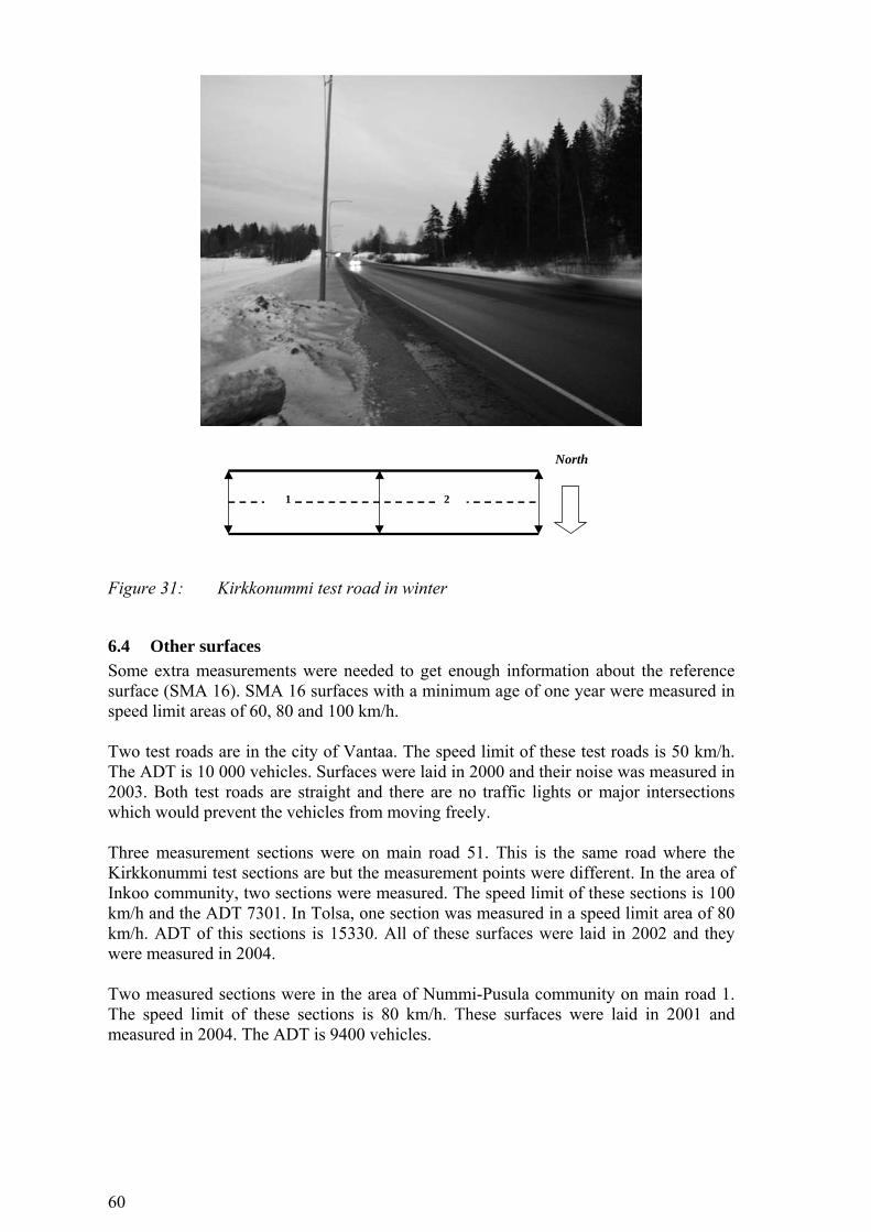
60

1 2

North

Figure 31: Kirkkonummi test road in winter

6.4 Other surfaces Some extra measurements were needed to get enough information about the reference surface (SMA 16). SMA 16 surfaces with a minimum age of one year were measured in speed limit areas of 60, 80 and 100 km/h. Two test roads are in the city of Vantaa. The speed limit of these test roads is 50 km/h. The ADT is 10 000 vehicles. Surfaces were laid in 2000 and their noise was measured in 2003. Both test roads are straight and there are no traffic lights or major intersections which would prevent the vehicles from moving freely. Three measurement sections were on main road 51. This is the same road where the Kirkkonummi test sections are but the measurement points were different. In the area of Inkoo community, two sections were measured. The speed limit of these sections is 100 km/h and the ADT 7301. In Tolsa, one section was measured in a speed limit area of 80 km/h. ADT of this sections is 15330. All of these surfaces were laid in 2002 and they were measured in 2004. Two measured sections were in the area of Nummi-Pusula community on main road 1. The speed limit of these sections is 80 km/h. These surfaces were laid in 2001 and measured in 2004. The ADT is 9400 vehicles.

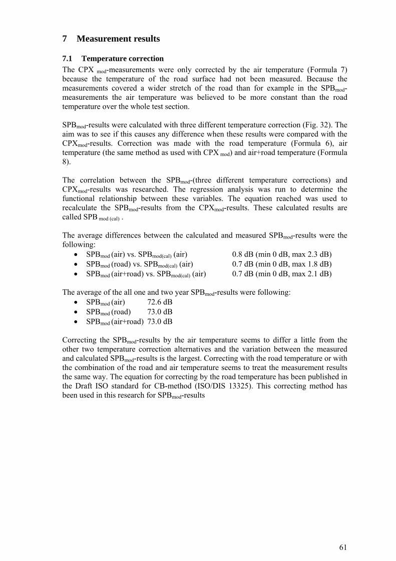
61

7 Measurement results

7.1 Temperature correction The CPX mod-measurements were only corrected by the air temperature (Formula 7) because the temperature of the road surface had not been measured. Because the measurements covered a wider stretch of the road than for example in the SPBmod-measurements the air temperature was believed to be more constant than the road temperature over the whole test section.

SPBmod-results were calculated with three different temperature correction (Fig. 32). The aim was to see if this causes any difference when these results were compared with the CPXmod-results. Correction was made with the road temperature (Formula 6), air temperature (the same method as used with CPX mod) and air+road temperature (Formula 8). The correlation between the SPBmod-(three different temperature corrections) and CPXmod-results was researched. The regression analysis was run to determine the functional relationship between these variables. The equation reached was used to recalculate the SPBmod-results from the CPXmod-results. These calculated results are called SPB mod (cal) . The average differences between the calculated and measured SPBmod-results were the following:

• SPBmod (air) vs. SPBmod(cal) (air) 0.8 dB (min 0 dB, max 2.3 dB) • SPBmod (road) vs. SPBmod(cal) (air) 0.7 dB (min 0 dB, max 1.8 dB) • SPBmod (air+road) vs. SPBmod(cal) (air) 0.7 dB (min 0 dB, max 2.1 dB)

The average of the all one and two year SPBmod-results were following:

• SPBmod (air) 72.6 dB • SPBmod (road) 73.0 dB • SPBmod (air+road) 73.0 dB

Correcting the SPBmod-results by the air temperature seems to differ a little from the other two temperature correction alternatives and the variation between the measured and calculated SPBmod-results is the largest. Correcting with the road temperature or with the combination of the road and air temperature seems to treat the measurement results the same way. The equation for correcting by the road temperature has been published in the Draft ISO standard for CB-method (ISO/DIS 13325). This correcting method has been used in this research for SPBmod-results

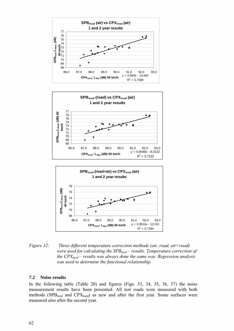
62

Figure 32: Three different temperature correction methods (air, road, air+road)

were used for calculating the SPBmod – results. Temperature correction of the CPXmod – results was always done the same way. Regression analysis was used to determine the functional relationship.

7.2 Noise results In the following table (Table 20) and figures (Figs. 33, 34, 35, 36, 37) the noise measurement results have been presented. All test roads were measured with both methods (SPBmod and CPXmod) as new and after the first year. Some surfaces were measured also after the second year.

SPBmod (air) vs CPXmod (air) 1 and 2 year results

y = 0,964x - 13,642R2 = 0,7308

68697071727374757677

86,0 87,0 88,0 89,0 90,0 91,0 92,0 93,0

CPXmod: LAeq (dB) 50 km/h

SPB m

od:L

Amax

(dB)

60

km

/h

SPBmod (road) vs CPXmod (air) 1 and 2 year results

y = 0,9048x - 8,0132R2 = 0,7133

68697071727374757677

86,0 87,0 88,0 89,0 90,0 91,0 92,0 93,0

CPXmod: LAeq (dB) 50 km/h

SPB

mod

:LAm

ax (d

B) 6

0 km

/h

SPBmod (road+air) vs CPXmod (air) 1 and 2 year results

y = 0,9516x - 12,201R2 = 0,7184

68

70

72

74

76

78

86,0 87,0 88,0 89,0 90,0 91,0 92,0 93,0CPXmod: LAeq (dB) 50 km/h

SPB m

od:L

Amax

(dB)

60 k

m/h

63

Some SPBmod – measurements did not succeed due to different reasons. This is further explained in chapter 7.3. Table 20: Results from the test roads . Test roads and tested products SPBmod : LAmax (dB) CPXmod; LAeq (dB)

New 1 year 2 years New 1 year 2 years Helsinki; SPBmod: 60 km/h CPXmod :50 km/h 1.Whisperphalt T + Whisperphalt B

- - - 86.5 90.1 -

2. Hiltti 3 + Hiltti 6 - - - 84.4 89.3 - 3.Viacodrän 11A + Viacobase 20B

- - - 87.7 91.8 91.0

4. HiljaT+Hilja A II - - - 86.1 90.6 - 5. Hiltti 3 + Hiltti 6 - - - 82.8 89.3 88.6 6. Hilja K + Hilja A - - - 85.3 90.1 - 7. Hilja OT - - - 82.5 87.8 - 8. Whisperphalt T - - - 84.3 90.8 - 9. SMA 6 - - - 84.3 88.8 88.4 10. Hilja OK - - - 86.5 - - 11. SMA 16 (ref) - - - 84.4 93.3 92.3 12. SMA 6 - - - 91.0 89.3 - Kaarina SPBmod: 60 km/h CPXmod :50 km/h 1. SMA 16 (ref) - 75.8 75.9 89.1 92.4 92.4 2. SMA 6 - 73.0 73.5 81.9 90.1 88.6 3. SMA 6 - 71.9 71.7 83.0 89.1 88.1 4. Whisperphalt T - 73.3 73.3 82.8 91.0 90.5 5. Novachip - 73.1 73.4 85.3 91.0 89.9 Kokkola SPBmod: 60 km/h CPXmod :50 km/h 1. SMA 8 71.5 73.6 - 85.2 90.2 - 2. SMA 5 70.3 73.5 - 83.9 89.1 - 3. SMA 18 72.6 76.0 - 89.5 92.1 - Espoo SPBmod: 60 km/h CPXmod :50 km/h 1. Novachip 8 65.8 73.3 - 82.5 89.4 - 2. Whisperphalt T 67.1 69.8 - 82.8 87.8 - 3. Hiltti-mix 69.6 72.8 - 85.1 88.0 - 4. SMA 6 69.1 71.6 - 83.6 87.4 - 5. Viacodrän 8 68.5 73.6 - 86.1 88.5 - 6. Viacodrän 11 71.5 72.2 - 89.9 88.5 - 7. SHP-Y 66.6 69.0 - 80.4 87.1 - 8. SHP-K2 68.1 72.0 - 82.6 88.3 - 9. SMA 8 (ref.) - - - 85.7 89.4 - 10. AC 16 (ref.) - - - 87.3 90.7 - Lohja SPBmod: 80 km/h CPXmod :50 km/h 1. AC 16 (ref.) 75.8 - - - 88.2 - 2. AC 16 (ref.) 76.5 - - - 87.9 - 3. Viacodrän 16 78.2 - - - 91.4 - 4. Viacodrän 11 75.9 - - - 89.5 - 5. Hiltti A 75.6 - - - 89.3 - 6. Hiltti F 74.3 - - - 86.3 - 7. SHP-KY 4 73.1 - - - 85.2 - 8. SHP-K3 73.0 - - - 85.5 - 9. Novachip 8 74.8 - - - 85.8 - 10. Novachip 11 77.6 - - - 91.2 - Kirkkonummi SPBmod: 100 km/h CPXmod :50 km/h 1. SMA 16 80.0 83.4 82.9 91.7 91.8 - 2. SMA 8 78.6 81.1 - 86.7 90.1 -

64

SPB mod; 60 km/h

40,0

45,0

50,0

55,0

60,0

65,0

70,0

75,0

80,0

1 (ref.) Kaarina

2 3 4 5 1 2 3 (ref.) Kokkola

1 Espoo

2 3 4 5 6 7 8

L(A

)max

(dB

)

New1 year2 years

Figure 33: SPBmod-results which were normalised to 60 km/h. Kaarina and Kokkola test sections were built in 2001 and Espoo test section in 2002.

SPB mod; 80 km/h

40,045,050,055,060,065,070,075,080,0

1 (ref.) Lohja

2 (ref.)

3 4 5 6 7 8 9 10

L(A

)max

(dB

)

New

Figure 34: SPBmod-results which were normalised to 80 km/h. Lohja test sections

were built in 2002.

65

SPBmod; 100 km/h

60,065,070,075,080,085,0

1(ref.)Kirkkonummi

2

L(A

)max

(dB

)

New1 year2 years

Figure 35: SPBmod-results which were normalised to 100 km/h. Kirkkonummi test

sections were built in 2002

CPXmod; 50 km/h

60,0

65,0

70,0

75,0

80,0

85,0

90,0

95,0

1 Helsinki

2 3 4 5 6 7 8 9 10 11 (ref.)

12 1 (ref.) Kaarina

2 3 4 5 1 (ref.) Kokkola

2 3

L(A

)eq

(dB

)

New 1 year 2 years

Figure 36: CPXmod-results from the test sections built in 2001. Measuring speed was

50 km/h.

66

.

CPXmod; 50 km/h

60,0

65,0

70,0

75,0

80,0

85,0

90,0

95,0

1 Espoo

2 3 4 5 6 7 8 9 (ref.)

10 (ref.)

1 (ref.) Lohja

2 (ref.)

3 4 5 6 7 8 9 10 1(ref.) Kirkkonum

mi

2

L(A)eq (dB)

New 1 year

Figure 37: CPXmod-results from the test sections built in 2002. Measuring speed was 50 km/h.

Some SMA 16-surfaces were measured at the different speed limit areas to fulfil the information gained from the test roads. These SPBmod-results have been presented in the following table. Table 21: SMA 16 results from other than test roads. Test sections and roads SPBmod ; LAmax (dB)

normalisation speed 60 km/h Vantaa 1 (Tikkurilantie) 75.9 Vantaa 2 (Länsimäentie) 75.4 normalisation speed 80 km/h Nummi-Pusula 1 (Main road 1) 80.0 Nummi-Pusula 2 (Main road 1) 80.0 Tolsa 1 (Main road 51) 79.5 normalisation speed 100 km/h Inkoo 1 (Main road 51) 83.6 Inkoo 2 (Main road 51) 83.6

7.3 Noise results from test roads not approved for the further investigation Test sections which are presented in this chapter did not give the noise information expected but they gave a lot of other information about the methods and quiet asphalt products. These results were not included in the research. • Helsinki; SPBmod-results The Helsinki test road was extremely difficult for SPBmod-measurements. It is a four lane road and there were curbs alongside the road. Sections were so short that finding a good or even a decent measuring site was difficult.

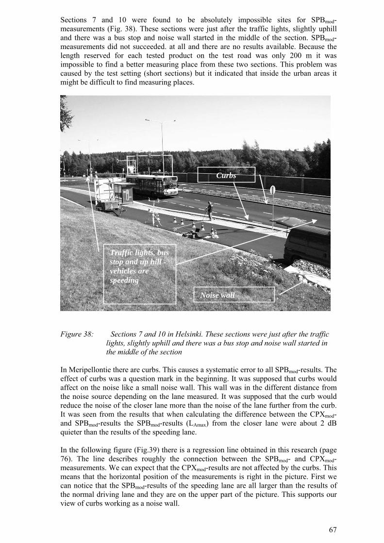
67

Sections 7 and 10 were found to be absolutely impossible sites for SPBmod-measurements (Fig. 38). These sections were just after the traffic lights, slightly uphill and there was a bus stop and noise wall started in the middle of the section. SPBmod-measurements did not succeeded. at all and there are no results available. Because the length reserved for each tested product on the test road was only 200 m it was impossible to find a better measuring place from these two sections. This problem was caused by the test setting (short sections) but it indicated that inside the urban areas it might be difficult to find measuring places.

Noise wall

Traffic lights, bus stop and up hill - vehicles are speeding

Curbs

Figure 38: Sections 7 and 10 in Helsinki. These sections were just after the traffic

lights, slightly uphill and there was a bus stop and noise wall started in the middle of the section

In Meripellontie there are curbs. This causes a systematic error to all SPBmod-results. The effect of curbs was a question mark in the beginning. It was supposed that curbs would affect on the noise like a small noise wall. This wall was in the different distance from the noise source depending on the lane measured. It was supposed that the curb would reduce the noise of the closer lane more than the noise of the lane further from the curb. It was seen from the results that when calculating the difference between the CPXmod- and SPBmod-results the SPBmod-results (LAmax) from the closer lane were about 2 dB quieter than the results of the speeding lane. In the following figure (Fig.39) there is a regression line obtained in this research (page 76). The line describes roughly the connection between the SPBmod- and CPXmod-measurements. We can expect that the CPXmod-results are not affected by the curbs. This means that the horizontal position of the measurements is right in the picture. First we can notice that the SPBmod-results of the speeding lane are all larger than the results of the normal driving lane and they are on the upper part of the picture. This supports our view of curbs working as a noise wall.

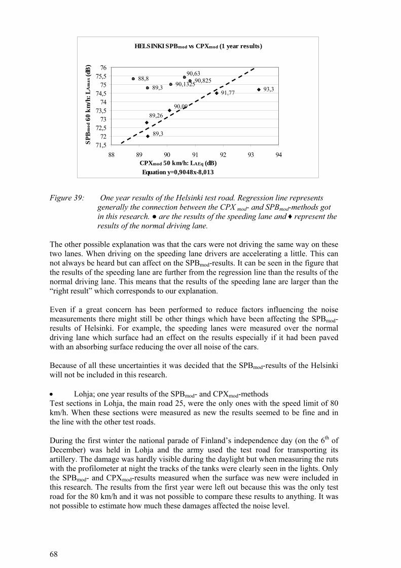
68

Figure 39: One year results of the Helsinki test road. Regression line represents

generally the connection between the CPX mod- and SPBmod-methods got in this research. ● are the results of the speeding lane and ♦ represent the results of the normal driving lane.

The other possible explanation was that the cars were not driving the same way on these two lanes. When driving on the speeding lane drivers are accelerating a little. This can not always be heard but can affect on the SPBmod-results. It can be seen in the figure that the results of the speeding lane are further from the regression line than the results of the normal driving lane. This means that the results of the speeding lane are larger than the “right result” which corresponds to our explanation. Even if a great concern has been performed to reduce factors influencing the noise measurements there might still be other things which have been affecting the SPBmod-results of Helsinki. For example, the speeding lanes were measured over the normal driving lane which surface had an effect on the results especially if it had been paved with an absorbing surface reducing the over all noise of the cars. Because of all these uncertainties it was decided that the SPBmod-results of the Helsinki will not be included in this research. • Lohja; one year results of the SPBmod- and CPXmod-methods Test sections in Lohja, the main road 25, were the only ones with the speed limit of 80 km/h. When these sections were measured as new the results seemed to be fine and in the line with the other test roads. During the first winter the national parade of Finland’s independence day (on the 6th of December) was held in Lohja and the army used the test road for transporting its artillery. The damage was hardly visible during the daylight but when measuring the ruts with the profilometer at night the tracks of the tanks were clearly seen in the lights. Only the SPBmod- and CPXmod-results measured when the surface was new were included in this research. The results from the first year were left out because this was the only test road for the 80 km/h and it was not possible to compare these results to anything. It was not possible to estimate how much these damages affected the noise level.

HELSINKI SPBmod vs CPXmod (1 year results)

91,7789,3 90,132590,82588,8

93,3

90,63

90,0989,26

89,3

71,572

72,573

73,574

74,575

75,576

88 89 90 91 92 93 94CPXmod 50 km/h: LAEq (dB)Equation y=0,9048x-8,013

SPB

mod

60

km/h

: LA

max

(dB

)

69

• Espoo; reference surfaces, SPBmod-method The standard (ISO 11819-1:1997) of the SPBmod-measurements says the following: “For the regression calculation and subsequent normalisation to a reference speed the following condition shall be met. The range of speeds covered by the measured vehicles shall be such that the reference speed shall be within the range of plus-or-minus one standard deviation from the actually measured average speed for heavy vehicles and plus-or-minus one-and-a-half standard deviation for cars.” The reference sections of Espoo (section 9 (SMA 8) and section 10 (AC 16)) could not meet this criteria neither when measured as new nor after the first year. The normalisation speed of the road was 60 km/h. The reference section 9 ends to the cross road and the reference section 10 starts from it. The cars were either speeding or reducing the speed on these sections. The SPBmod-results of Espoo sections 9 and 10 will not be further investigated in this research. • Kaarina; first year SPBmod-results Test roads were measured first time in the end of October in 2001. The weather was already quite cold also during the day time. The air temperature varied from 0.6 to 5.6 ºC. The most of the measurements were done under the limit set in the ISO-standard. First year SPBmod-results from Kaarina were left out of this research.

7.4 Wearing results Prall-test was done for the core samples from two test roads: Helsinki and Kaarina. Results were following: Table 22: Prall-results from Kaarina and Helsinki test roads Section Prall-value

(average; cm3) Numb. of sound samples1)

Helsinki 1.WhisperphaltT+Whisperphalt B 19.4 6 2.& 5. Hiltti 3 + Hiltti 6 35.2 3+1 3. Viacodrän 11A+Viacobase 20B - 4 4. HiljaT+Hilja A 11 42.2 3 6. Hilja K + Hilja A 38.4 6 7. Hilja OT 56.2 4 8. Whisperphalt T 16.7 6 9.& 12. SMA 6 25.0 2+4 10. Hilja OK 34.6 6 11. SMA 16 (ref) 21.0 6

Kaarina 1. SMA 16 (ref) 27.7 1 2. SMA 6 79.4 5 3. SMA 6 31.0 6 4. Whisperphalt T 32.5 2 5. Novachip 64.7 6 1)Totally six samples were ran from each section but some of them got broke during the test. Average was calculated from the sound samples Following test roads were measured with the profilometer: Helsinki, Kaarina, Espoo and Lohja. Results of the Helsinki test road were corrected by the traffic volume (only light vehicles using studded tyres) because the traffic volume changed remarkably on the different sections of the test road. Volumes were corrected by the reference surface 11. On the other test roads the variation was so small that it did not affect the results and

70

they were not corrected. Only the results from the same test road can be compared with each other. The deformation and wearing of surfaces can be seen from the following tables: Wearing: autumn measurement (before the use of the studded tyres starts)-spring measurement (after the period of studded tyres) Deformation: spring measurement (after the period of studded tyres)-autumn measurement (before the use of the studded tyres starts) Rutting: wearing + deformation Table 23: Traffic volume corrected profilometer-results of Helsinki. Section Traffic

volume (light

vehicles)

Traffic volume

correction coefficient

Autumn 01

Spring 02

Autumn 02

Spring 03

Helsinki; traffic volume corrected ruts [mm] 1.Whisperphalt T + Whisperphalt B

6080 0.862 1.5 15.4 15.5 not measured

2. Hiltti 3 + Hiltti 6 6953 0.986 0.8 6.1 6.3 13.4 3.Viacodrän 11A + Viacobase 20B

7260 1.029 2.7 4.6 4.7 6.4

4. HiljaT+Hilja A II 4748 0.673 1.7 4.3 4.9 8.1 5. Hiltti 3 + Hiltti 6 4662 0.661 2.9 7.9 8.3 14.2 6. Hilja K + Hilja A 4021 0.570 3.7 6.9 7.3 11.9 7. Hilja OT 4701 0.667 3.4 14.2 14.6 24.1 8. Whisperphalt T 4360 0.618 3.1 17.1 17.7 33.3 9. SMA 6 3986 0.565 3.6 6.5 7.0 9.3 10. Hilja OK 6858 0.972 2.6 6.1 6.2 10.8 11. SMA 16 (ref) 7053 1.000 2.4 3.7 3.9 5.1 12. SMA 6 7188 1.019 2.2 7.6 8.0 13.4 Table 24: Profilometer-results of Kaarina Section Autumn 01 Spring 02 Autumn 02 Spring 03 Kaarina; ruts [mm] 1. SMA 16 (ref) 2.3 5.4 6.7 7.3 2. SMA 6 0.9 7.7 8.8 14.4 3. SMA 6 2.0 4.1 4.9 6.7 4. Whisperphalt T 2.0 5.6 6.3 10.1 5. Novachip 2.0 6.8 7.6 10.7 Table 25: Profilometer-results of Espoo Section Autumn 02 Spring 03 Espoo; ruts [mm] 1. Novachip 8 1.7 5.4 2. Whisperphalt T 0.9 3.6 3. Hiltti-mix 1.5 3.1 4. SMA 6 0.7 2.8 5. Viacodrän 8 1.4 2.7 6. Viacodrän 11 2.4 3.5 7. SHP-Y 1.0 5.1 8. SHP-K2 1.3 3.5 9. SMA 8 (ref.) 0.7 2.6 10. AC 16 (ref.) 1.4 4.1

71

Table 26: Profilometer-results of Lohja Section Autumn 02 Spring 03 Lohja; ruts [mm] 1. AC 16 (ref.) 1.0 3.0 2. AC 16 (ref.) 1.1 3.6 3. Viacodrän 16 2.1 3.6 4. Viacodrän 11 1.2 4.2 5. Hiltti A 1.4 2.3 6. Hiltti F 1.2 3.6 7. SHP-KY 4 1.5 4.1 8. SHP-K3 1.3 5.6 9. Novachip 8 4.0 8.6 10. Novachip 11 3.0 9.3

72

8 Evaluation of methods for quiet surfaces

8.1 Choosing the method

8.1.1 Repeatability of the SPBmod- and CPXmod-methods Wrong calibration of the measurement devices can cause systematic error to the results. According to SPB ISO standard [ISO 11819-1] this error can be ±1 dB. The other uncertainty is the composition of the vehicle fleet which can change from place to place and time to time. This can cause the 0.3-0.6 dB systematic error to the results [ISO 11819-1] . It is also suggested that the measurements should be done close to the reference temperature ( +20 °C) to avoid the uncertainties included in the corrections. According to the standard [ISO 11819-1] expected random errors in A-weighted sound pressure levels are as presented in the following table 27. The errors quantified in the table represent road categories “medium” and “high”. The measurements made in the road speed category “low” may be influenced more by driving behaviour than others (some vehicles may be in an acceleration or deceleration mode which is not always easy to note). According to the standard the repeatability of the SPB-measurements is better than 1.0 dB. [ISO 11819-1] Table 27: Expected random errors in A-weighted sound pressure level. [ISO 11819-1] Vehicle class Standard deviation for

individual vehicles around Lveh

95 % confidence interval around Lveh

Cars 1.5 dB 0.3 dB Heavy vehicles, dual-axle 2.0 dB 0.7 dB Heavy vehicles, multi-axle 2.0 dB 0.7 dB NOTE-The confidence intervals, around the Vehicle Sound Levels, assume that the number of vehicles is 100 cars and 40 heavy vehicles of each type. The corresponding random error of the SPBI will be a combination of these errors according to the chosen weighting factors. The repeatability of the SPBmod–method was tested at two test sections: Espoo 3 and Kokkola 1. Test sections were measured totally five times. On both test roads measurements were done during three different days. The results are in the following figure (Fig. 40).

73

Figure 40: Five repeated measurements were done on two test roads: Kokkola

section 1 and Espoo section 3. In this research only the cars were included and the repeated measurements were done in the category “low”. The difference between the smallest and largest value is 0.2 dB in Espoo and 1.2 dB in Kokkola. One measurement in Kokkola is 0.5 dB lower than the second lowest. It is difficult to estimate the reason for that but it is possible that there has been some kind of mistake in the measurement event or the malfunctioning of the devices. This measurement was done at the same day as the previous measurement (73.9 dB) and just after that. Devices were rebuilt again for the second measurement. Weather conditions were about the same during these two measurement. If this measurement is left out the difference between the smallest and largest value is 0.7 dB. The standard gives the repeatability value of “better than 1 dB” for SPB-measurements in the categories “medium” and “high”. When heavy vehicles have been left out it could be estimated that the repeatability is somewhat better because in the category of cars the standard deviations are smaller. These results show that also in Finland we can meet this same repeatability. The repeated measures done in this research were done just to check the repeatability given in the standard. When doing the evaluation measurements each test section should be measured two times. If the difference between these two measurements is larger than 1 dB third measurement should be done to avoid the unnoticed mistakes during the measurements. In Kirkkonummi the test sections were long enough so that it was possible to measure the same surface, SMA 8, from three different spots (Fig. 41). Test spots 2 and 3 were about 200 meters from the original measurement point 1. Test road was straight and test sections as well as the weather conditions were almost identical during the measurements. The difference between the LAmax minimum and maximum value was 0.4 dB. Changing the measurement spot does not seem to influence the results critically.

Repeated measurements in the same place (SPBmod)

73,6

73,1

74,2

72,7

73,974,3

72,672,672,8 72,8

72

73

74

75

L Am

ax (d

B)

Espoo 3 Kokkola 1

74

Figure 41: Kirkkonummi SMA 8 results (1 year old) measured from three different

spots. The repeatability of 1 dB for SPBmod-measurements can be used. The vehicles used in Finland are older than in the other European countries. Their average age is about 10.4 years and the average scabbing age is 18 years. This can cause difference when comparing with the results measured in the other countries. This should also been kept in mind after a few years if the Finnish vehicle fleet renews and today’s measurements will be compared with them. CPXmod-measurements were done by the Laboratory of Automotive Engineering (HUT) and with NOTRA-trailer. This trailer has been used earlier in the same kinds of measurements. In the internal memo of the laboratory [TKK Autolaboratorio, (2001)] the calculated total uncertainty of the method was 1.0 %. If the highest measured sound pressure level is 105 dB this equals 1 dB. [TKK Autolaboratorio (2001)] The repeatability of 1 dB for CPXmod-measurements can be used.

8.1.2 Comparing the SPBmod- and CPXmod – results If these two methods would treat these surfaces the same way, either of these methods could be used for testing the noise qualities of surfaces. So far the connection found between the two original methods has not covered all the surface types. In this research the methods used were modified as explained earlier. In the figure 42 we can see how these two methods put surfaces in the order of magnitude depending on the noise measured. One and two year (2y) results from the Kaarina, Kokkola and Espoo test roads are presented. SPBmod-results are in the darker columns in the order of magnitude. Corresponding CPXmod-results are marked with a lighter colour.

Kirkkonummi SMA 8 Measurements in different places (SPBmod)

81,1 80,9 80,7

77

78

79

80

81

82

1 2 3

L A m

ax (d

B)

75

68

70

72

74

76

78

80

82

84

86

88

90

92

94

SPBmod 76 75,9 75,8 73,6 73,6 73,5 73,5 73,4 73,3 73,3 73,3 73,1 73 72,8 72,2 72 71,9 71,7 71,6 69,8 69

CPXmod 92,1 92,4 92,4 88,5 90,2 89,1 88,6 89,9 89,4 91 90,5 91 90,1 88 88,5 88,3 89,1 88,1 87,4 87,8 87,1

Ko 3 Ka 1 2y

Ka 1 Es 5 Ko 1 Ko 2 Ka 2 2y

Ka 5 2y

Es1 Ka 4 Ka 4 2y

Ka 5 Ka 2 Es 3 Es 6 Es 8 Ka 3 Ka 3 2y

Es 4 Es 2 Es7

LAm ax,LAe q

(dB)

Figure 42: One and two year (2y) old surfaces on Kokkola (Ko), Kaarina (Ka) and

Espoo (Es) test roads in the order of noisiness (SPBmod-method ). The difference between the highest and lowest value is larger when measured with the SPBmod-method (SPBmod 7dB and CPXmod 5.3 dB). Both methods find the same three noisiest surfaces (Kokkola 3 and Kaarina 1; 1 and 2 years). Both methods find the three noisiest surfaces clearly noisier than the other surfaces. This was expected, because these three surfaces were “reference” surfaces SMA 16 (Kaarina 1, 1 and 2 years) and SMA 18 (Kokkola 3). With the SPBmod-method these surfaces are over 2 dB noisier than the next surfaces and with the CPXmod-method there is about 1 dB difference to the next noisiest surface. The three most quiet surfaces (Espoo 2 years, sections 4 and 7) were also found with both methods. It should be noticed though that when measured with the SPBmod-method two most quiet surfaces Espoo 2 and 7 are about 2 dB (difference 2.6-1.8 dB) quieter than Espoo 4. CPXmod-method finds these three surfaces almost equally quiet (difference 0.8 dB). Espoo 6 and 8 as well as Kaarina 3 (1 and two years) are almost equally treated with these two methods. The difference between the noisiest of them and the most quiet of them is inside the repeatability (SPBmod 0.5 dB and CPXmod 1.0 dB). The SPBmod-results between 72.8-73.6 dB are interesting. These are well inside the repeatability of SPBmod-method so they could be easily in a different order. When these sections were measured with the CPXmod-method the results spread over a wide range of decibels (88.0-91 dB) (these are shown inside the squares). It can be seen that the CPXmod-method finds differences between the certain surfaces that can not be heard from the roadside. SPBmod-method separates the “reference” surfaces clearly from the “quiet surfaces”. Also the most quiet surfaces are clearly quieter than the other surfaces. CPXmod-method

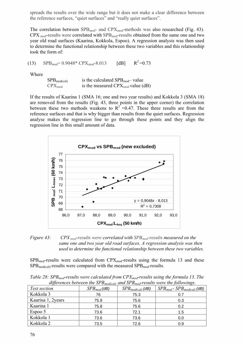
76

spreads the results over the wide range but it does not make a clear difference between the reference surfaces, “quiet surfaces” and “really quiet surfaces”. The correlation between SPBmod- and CPXmod-methods was also researched (Fig. 43). CPX mod-results were correlated with SPBmod-results obtained from the same one and two year old road surfaces (Kaarina, Kokkola, Espoo). A regression analysis was then used to determine the functional relationship between these two variables and this relationship took the form of:

(13) SPBmod= 0.9048* CPXmod-8.013 [dB] R2 =0.73 Where

SPBmod(cal) is the calculated SPBmod– value CPXmod is the measured CPXmod-value (dB) If the results of Kaarina 1 (SMA 16; one and two year results) and Kokkola 3 (SMA 18) are removed from the results (Fig. 43, three points in the upper corner) the correlation between these two methods weakens to R2 =0.47. These three results are from the reference surfaces and that is why bigger than results from the quiet surfaces. Regression analyse makes the regression line to go through these points and they align the regression line in this small amount of data. Figure 43: CPX mod-results were correlated with SPBmod-results measured on the

same one and two year old road surfaces. A regression analysis was then used to determine the functional relationship between these two variables.

SPBmod-results were calculated from CPXmod-results using the formula 13 and these SPBmod(cal)-results were compared with the measured SPBmod-results. Table 28: SPBmod-results were calculated from CPXmod-results using the formula 13. The

differences between the SPBmod(cal) and SPBmod-results were the followings. Test section SPBmod (dB) SPBmod(cal) (dB) SPBmod - SPBmod(cal) (dB)Kokkola 3 76 75.3 0.7 Kaarina 1, 2years 75.9 75.6 0.3 Kaarina 1 75.8 75.6 0.2 Espoo 5 73.6 72.1 1.5 Kokkola 1 73.6 73.6 0.0 Kokkola 2 73.5 72.6 0.9

y = 0,9048x - 8,013R2 = 0,7308

68697071727374757677

86,0 87,0 88,0 89,0 90,0 91,0 92,0 93,0

CPXmod:LAeq (50 km/h)

SPB

mod

: LA

max

(60

km/h

)

CPXmod vs SPBmod (new excluded)

77

Kaarina 2, 2 years 73.5 72.2 1.3 Kaarina 5, 2years 73.4 73.3 0.1 Espoo 1 73.3 72.9 0.4 Kaarina 4 73.3 74.3 -1.0 Kaarina 4, 2 years 73.3 73.9 -0.6 Kaarina 5 73.1 74.3 -1.2 Kaarina 2 73 73.5 -0.5 Espoo 3 72.8 71.6 1.2 Espoo 6 72.2 72.1 0.1 Espoo 8 72 71.9 0.1 Kaarina 3 71.9 72.6 -0.7 Kaarina 3, 2 years 71.7 71.7 0.0 Espoo 4 71.6 71.1 0.5 Espoo 2 69.8 71.4 -1.6 Espoo 7 69 70.8 -1.8 The difference between the measured and calculated results was one or over one decibel on the following sections: • Espoo 2 • Espoo 3 • Espoo 5 • Espoo 7 • Kaarina 4 (1 year) • Kaarina 5 (1year) • Kaarina 2 (2 years) According to the figure 42 these differences were expected. Espoo, sections 2 and 7, were obvious outliers because SPBmod-method finds them clearly quieter than the others surfaces when CPXmod-method does not find any major difference between these and the other “quiet surfaces”. The other outliers were well inside 1dB when measured with the SPBmod-method when their CPXmod-results spread over 2.5 dB. It seems that even these two modified methods do not correlate with each other on the level high enough. Good correlation would have allowed us to use these methods as parallel. Number of results was not significant in this research to make clear statements but it did not give any more promising results than those obtained with non-modified SPB- and CPX-methods.

8.1.3 Suggestion for the noise measurement method SPB mod- and CPXmod-methods should not be used to compensate each other as such. They correlate with each other in a certain level but not with all surfaces. Both of them have advantages and which should be exploited. SPB-method has been widely used for testing surfaces in the other countries and for type testing in some. This modified version, SPBmod, follows the standard quite closely. Only the heavy vehicles were left out and the normalisation speeds differ a little from the suggested. SPBmod-method can and should be used for type testing the noise properties of surfaces in Finland. Repeatability of the SPBmod-method is 1 dB. CPX mod-method can be used for product conformity checking as long stretches of roads can be measured.

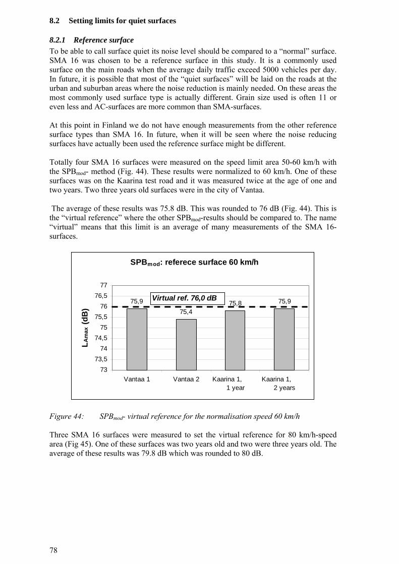
78

8.2 Setting limits for quiet surfaces

8.2.1 Reference surface To be able to call surface quiet its noise level should be compared to a “normal” surface. SMA 16 was chosen to be a reference surface in this study. It is a commonly used surface on the main roads when the average daily traffic exceed 5000 vehicles per day. In future, it is possible that most of the “quiet surfaces” will be laid on the roads at the urban and suburban areas where the noise reduction is mainly needed. On these areas the most commonly used surface type is actually different. Grain size used is often 11 or even less and AC-surfaces are more common than SMA-surfaces. At this point in Finland we do not have enough measurements from the other reference surface types than SMA 16. In future, when it will be seen where the noise reducing surfaces have actually been used the reference surface might be different. Totally four SMA 16 surfaces were measured on the speed limit area 50-60 km/h with the SPBmod- method (Fig. 44). These results were normalized to 60 km/h. One of these surfaces was on the Kaarina test road and it was measured twice at the age of one and two years. Two three years old surfaces were in the city of Vantaa. The average of these results was 75.8 dB. This was rounded to 76 dB (Fig. 44). This is the “virtual reference” where the other SPBmod-results should be compared to. The name “virtual” means that this limit is an average of many measurements of the SMA 16-surfaces.

SPBmod: referece surface 60 km/h

75,975,4

75,8 75,9

7373,5

7474,5

7575,5

7676,5

77

Vantaa 1 Vantaa 2 Kaarina 1, 1 year

Kaarina 1, 2 years

L Am

ax (d

B)

Virtual ref. 76,0 dB

Figure 44: SPBmod- virtual reference for the normalisation speed 60 km/h Three SMA 16 surfaces were measured to set the virtual reference for 80 km/h-speed area (Fig 45). One of these surfaces was two years old and two were three years old. The average of these results was 79.8 dB which was rounded to 80 dB.

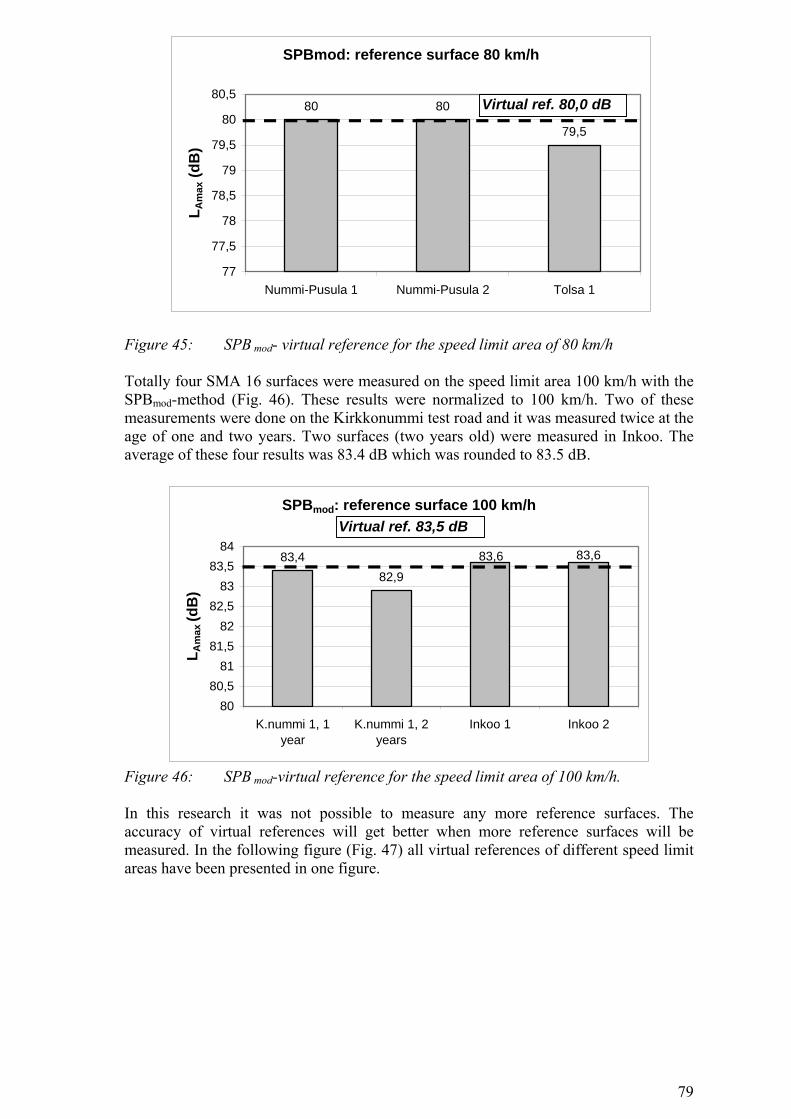
79

SPBmod: reference surface 80 km/h

80 80

79,5

77

77,5

78

78,5

79

79,5

80

80,5

Nummi-Pusula 1 Nummi-Pusula 2 Tolsa 1

L Am

ax (d

B)

Virtual ref. 80,0 dB

Figure 45: SPB mod- virtual reference for the speed limit area of 80 km/h Totally four SMA 16 surfaces were measured on the speed limit area 100 km/h with the SPBmod-method (Fig. 46). These results were normalized to 100 km/h. Two of these measurements were done on the Kirkkonummi test road and it was measured twice at the age of one and two years. Two surfaces (two years old) were measured in Inkoo. The average of these four results was 83.4 dB which was rounded to 83.5 dB.

SPBmod: reference surface 100 km/h

83,482,9

83,683,6

8080,5

8181,5

8282,5

8383,5

84

K.nummi 1, 1year

K.nummi 1, 2years

Inkoo 1 Inkoo 2

L Am

ax (d

B)

Virtual ref. 83,5 dB

Figure 46: SPB mod-virtual reference for the speed limit area of 100 km/h. In this research it was not possible to measure any more reference surfaces. The accuracy of virtual references will get better when more reference surfaces will be measured. In the following figure (Fig. 47) all virtual references of different speed limit areas have been presented in one figure.

80

SPBmod: Virtual References

76

80

83,5

72

74

76

78

80

82

84

86

60 80 100

km/h

L Am

ax (d

B)

Figure 47: Virtual references of different normalisation speeds.

8.2.2 Definition of the quiet surface All the surfaces which noise is less than the noise of the reference surface could be named quiet surfaces. However, this is not very practical solution. How much reduction should be required for the quiet surface? The repeatability of the SPBmod-method is 1 dB so the reduction should be more than this. Commonly used definition has been -3 dB and it defends its place as it equals 50 % reduction in the amount of traffic or the reduction of the speed limit by 20 km/h which are both radical actions. However, in this research there were products which were 7 dB quieter than the virtual reference in the speed limit area of 60 km/h. Definition should give a full credit also to these products. This could be achieved by having several categories. For example, “quiet surface”, “extra quiet surface” and “super quiet surface” with appropriate decibel limits for each speed limit area. This research did not give enough measurement data for this approach. Noise level is only a one character of a surface. When choosing a surface a decisions are made based on price and different qualities as resistance to wear, noise level etc. Instead of setting strict dB-limits for quiet surfaces each work site should have a targeting noise level. Weather this can be achieved with a surface or with the combination of surface and other noise abatement structures should be decided case-based. This approach gives full credit to the products which reduce noise more than for example 3 dB. Noise levels of the different products can be expressed by comparing them to the virtual references.

8.3 The durability of noise reduction In the early experiments of the quiet surfaces in Finland the fast loss of noise reduction was reported (see Annex 1). Different surfaces behave differently during the first year. In this research the changes in the noise level vary from 0 up to 8.1 dB. The first measurements were done two weeks after the laying at the earliest. During the first winter surfaces seem to take their acoustical level that they keep for a few years. We can say that during the first year some surfaces perform extra noise reduction and give extra benefit. Some of the test sections built in 2001 were measured also in 2003 after the second winter. It was feared that studded tyres used in Finland might increase the noise winter after winter. The surfaces achieved their acoustical level during the first winter and after

81

that it was maintained (Fig. 48) over the second winter season. This result was quite promising and at least showed that the acoustical properties did not disappear during the first winters. More experience is not available from these test roads. Due to the international experiences (see chapter 3.2.5) the acoustical properties of the surfaces have remained for some years but these results are not from the test roads where the studded tyres have been used. Figure 48: One and two year results from the two test roads.

8.4 Prall-test and its modification Running the Prall-test for the noise reducing pavements was difficult. Some of the core samples were fretting strongly and especially the edges of the samples did not last. Results were counted from the core samples which stayed as whole. Results showed that the Prall-test did not predict the actual wearing of the surfaces (Fig. 49). The result was almost the opposite: those surfaces which did fine in the Prall-test did not last at all on the road and vice versa.

70,0

72,0

74,0

76,0

78,0

80,0

82,0

84,0

86,0

88,0

90,0

92,0

94,0

96,0

SPB

Kaarina 1

2 3 4 5 CPX

Kaarina 1

2 3 4 5 Helsinki 3

5 7 9 11

SPB

: LA

max

(dB

)/ C

PX: L

Aeq

(dB

)

New One year Two years

82

Figure 49: Prall-results did not predict the actual wearing. Bigger the Prall-result

was more wearing was expected on the road. The result was almost the opposite.

It was suspected that rubberised bitumen would have an effect on the Prall-results (it must be remembered that the recipes of the tested surfaces were not known). Steel balls used in the test do not scratch the surface at all like the studs do in the real environment. The other problem was that Prall-test was too “rough” for quiet surfaces. Core samples did not last whole in the test which was ran with the normal settings. The Prall-test was modified so that the samples would stay whole. This time the proportioning of the asphalt mixtures was done in the Laboratory of the Highway Engineering (HUT) so that it was known. Also the samples were done in the laboratory with the ICT. Following asphalt types were tested. • SMA 5 (representing the fine grain type of quiet surfaces) • OA 11 (representing the open type of quiet surfaces) • SMA 16 (reference) Some samples were also made with the rubberised bitumen. The first aim was to find right settings so that the core samples would stay whole. Rotation frequency was lowered little by little (850→ 750→650→600 rpm). An appropriate frequency was 600 rpm. Samples from all mass types stayed whole. Anyhow, this rotation frequency was so low that the samples did not wear much in 15 minutes. The time of the test was added by half to 30 minutes. These settings were used for some core samples drilled from the Espoo test road. Because the recipes of the samples were unknown contractors were asked weather their products included rubberised bitumen or not. It was believed that the rubberised bitumen could cause some problems with the results. During the normal Prall-test it seemed that the rubberised bitumen caused a protecting cover on the top of the sample. In a short test setting we tried to add the water flow from 2 l/minute. The aim was to “wash” the cover away. This did not work the way we expected. More water we added less the sample

Helsinki: Prall-value vs wearingAutumn 2001 – Spring 2002

0 2 4 6 8

10 12 14 16

16.7 19.4 21 25 25 34.6 35.2 35.2 38.4 42.2 56.2 Prall-value (cm3)

Wea

ring

(mm

)

83

wore. We decided to keep the water flow in 2 l/minute and pay attention to the samples including rubberised bitumen when running the tests. In the following figure (Fig. 50), it can be seen how the rubberised bitumen forms a sheltering cover on the top of the sample and how the samples got broken even though the rotation frequency was already lowered.

Figure 50: On the left: SMA 5 sample with rubberised bitumen. Bitumen has formed

a sheltering cover on the top of the sample. In the middle: open graded asphalt (OA11) after the modified Prall-test (750 rpm/15 minutes). Still the edges of the sample broke. On the right: open graded asphalt (OA11) after the modified Prall-test (600 rpm/15 minutes). Sample has stayed whole but did not wear much. After this the testing time was added to 30 min.

Modified Prall-test was done for the core samples drilled from the Espoo test road. These results were compared with the profilometer results from the same road to see if the modified Prall-test could predict the actual wearing (Table 29 and Fig. 51). Table 29: The comparison of the results of the modified Prall-test (600 rpm, 30 min) and

the actual wearing measured from the Espoo test road after the first winter. Test section Modified Prall-value

(cm3) Wearing (mm)

1 25.5 3.7 2 10.9 2.7 3 7.8 1.6 4 9.7 2.1 5 14.5 1.3 6 11.7 1.1 7 8.3 4.1 8 16.1 2.2 9 20.7 1.9 10 21.6 2.7

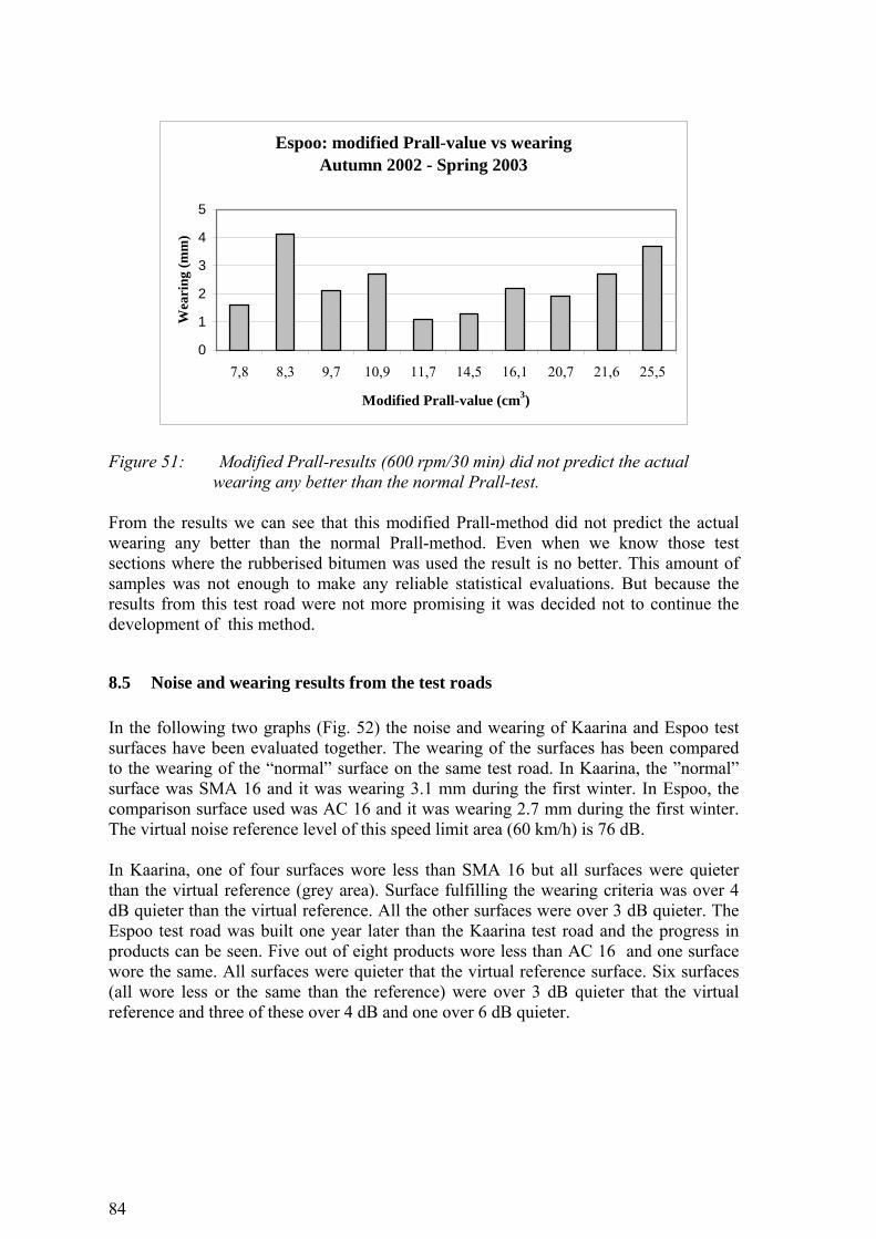
84

Espoo: modified Prall-value vs wearingAutumn 2002 - Spring 2003

0

1

2

3

4

5

7,8 8,3 9,7 10,9 11,7 14,5 16,1 20,7 21,6 25,5

Modified Prall-value (cm3)

Wea

ring

(mm

)

Figure 51: Modified Prall-results (600 rpm/30 min) did not predict the actual

wearing any better than the normal Prall-test. From the results we can see that this modified Prall-method did not predict the actual wearing any better than the normal Prall-method. Even when we know those test sections where the rubberised bitumen was used the result is no better. This amount of samples was not enough to make any reliable statistical evaluations. But because the results from this test road were not more promising it was decided not to continue the development of this method.

8.5 Noise and wearing results from the test roads In the following two graphs (Fig. 52) the noise and wearing of Kaarina and Espoo test surfaces have been evaluated together. The wearing of the surfaces has been compared to the wearing of the “normal” surface on the same test road. In Kaarina, the ”normal” surface was SMA 16 and it was wearing 3.1 mm during the first winter. In Espoo, the comparison surface used was AC 16 and it was wearing 2.7 mm during the first winter. The virtual noise reference level of this speed limit area (60 km/h) is 76 dB. In Kaarina, one of four surfaces wore less than SMA 16 but all surfaces were quieter than the virtual reference (grey area). Surface fulfilling the wearing criteria was over 4 dB quieter than the virtual reference. All the other surfaces were over 3 dB quieter. The Espoo test road was built one year later than the Kaarina test road and the progress in products can be seen. Five out of eight products wore less than AC 16 and one surface wore the same. All surfaces were quieter that the virtual reference surface. Six surfaces (all wore less or the same than the reference) were over 3 dB quieter that the virtual reference and three of these over 4 dB and one over 6 dB quieter.

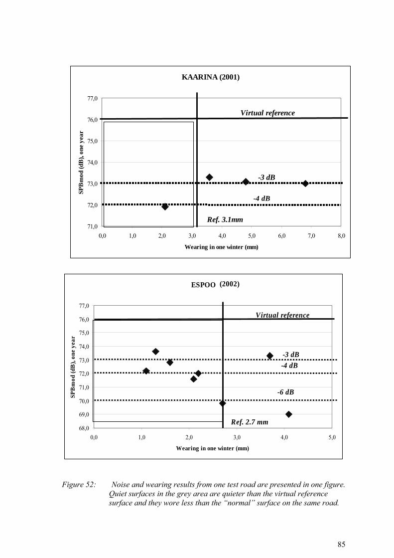
85

Figure 52: Noise and wearing results from one test road are presented in one figure.

Quiet surfaces in the grey area are quieter than the virtual reference surface and they wore less than the “normal” surface on the same road.

ESPOO

68,0

69,0

70,0

71,0

72,0

73,0

74,0

75,0

76,0

77,0

0,0 1,0 2,0 3,0 4,0 5,0

Wearing in one winter (mm)

SPB

mod

(dB

), on

e ye

ar

Ref. 2.7 mm

Virtual reference

-3 dB

-6 dB

-4 dB

(2002)

KAARINA (2001)

71,0

72,0

73,0

74,0

75,0

76,0

77,0

0,0 1,0 2,0 3,0 4,0 5,0 6,0 7,0 8,0

Wearing in one winter (mm)

SPB

mod

(dB

), on

e ye

ar

-4 dB

Ref. 3.1mm

Virtual reference

-3 dB

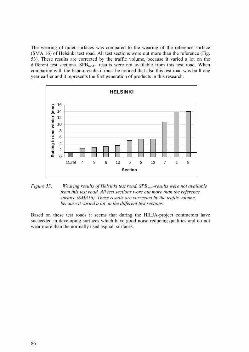
86

The wearing of quiet surfaces was compared to the wearing of the reference surface (SMA 16) of Helsinki test road. All test sections wore out more than the reference (Fig. 53). These results are corrected by the traffic volume, because it varied a lot on the different test sections. SPBmod– results were not available from this test road. When comparing with the Espoo results it must be noticed that also this test road was built one year earlier and it represents the first generation of products in this research. Figure 53: Wearing results of Helsinki test road. SPBmod-results were not available

from this test road. All test sections wore out more than the reference surface (SMA16). These results are corrected by the traffic volume, because it varied a lot on the different test sections.

Based on these test roads it seems that during the HILJA-project contractors have succeeded in developing surfaces which have good noise reducing qualities and do not wear more than the normally used asphalt surfaces.

HELSINKI

02468

10121416

11,ref 4 9 6 10 5 2 12 7 1 8

Section

Rut

ting

in o

ne w

inte

r (m

m)

87

9 Opinions about quiet surfaces and their future use

9.1 Enquiry for big cities and Road Districts An enquiry about the use of the quiet asphalt surfaces (Annex 1) was sent to 16 large cities in different parts of Finland. Cities are responsible for paving their own street network. The Finnish Road Administration has nine local Road Districts (Tiepiiri) responsible for the public roads in their area. This enquiry was sent to them as well. Eight Road Districts and 14 cities answered the enquiry. Answers can be see in detail in Annex 1. Seven Road Districts out of eight had used surfaces for reducing noise in their area. Products they had used were SMA 5-11, OA 8, TINO and some experimental surfaces. Only four cities had used quiet surfaces and two of them had HILJA-test roads in their area. Besides the products tested in the HILJA-project the cities had also used SMA, porous asphalts and Novachip. Surfaces had been used the following way: Table 30: Usage of quiet surfaces in the area of eight Road Districts and 14 cities Road Districts (m2) Cities (m2) Before year 1999 7 000 20 000 Year 2000 58 719 9000 Year 2001 199 700 20 000 Year 2002 158 930 58 200 Total 424 346 107 200 Total (Road District & cities)

531 546 m2

Quiet surfaces were used on the roads the following way: Four lane roads: ADT> 15 000 even ADT 50 000 Two lane roads: ADT about 3000-10 000 Speed limit varied from 60 km/h to 100 km/h. In the cities surfaces had been used on the streets where ADT was 12 000-20 000 and the speed limit 50-80 km/h. Early experiments indicated that quiet surfaces were rutting fast and after the first year the noise reduction properties seemed to disappear. Only the city of Oulu stated that the surface did not rut much when used in city area (ADT 17 000, speed limit 50 km/h). Cities mentioned that they got positive feedback from users. Four cities which had used quiet surfaces said that they will use them in the future as well. From the other ten cities four said that they will use quiet surfaces, one said maybe and three cities said no. Two cities did not answer this question at all. Out of the eight Road Districts, five will use quiet surfaces in future. One answered no (or maybe) and two did not answer this question. It was asked, what would be the best way for the road authorities or cities to order quiet surfaces in future and three alternatives were suggested.

88

1. Products will be tested beforehand and a certificate which states that the product is quiet will be given.

2. Noise and wearing properties will be measured after the first year and either penalty fees or bonuses will be paid depending on how the product fills the requirements set.

3. Noise and rutting properties have a long guarantee time (2-3 years). This question got 17 answers. All three alternatives were supported. Alternative 3 was supported by 6, alternative 1 by two and alternative 2 was supported by one. It was also said that none of these alternatives is enough alone. Using all three (2), or combining the pre-qualification with a long guarantee time (2) or long guarantee time with the first year testing (4) were suggested as well. It seems that the main concerns have been the rutting of the surfaces and the fact that the noise reducing propertied disappeared after a few years. At the same time these surfaces had been used on the roads with quite heavy traffic. There was not much experience from the low traffic roads on the residential areas. Anyway, there was positive indication that these surfaces might be used in future as well.

9.2 HILJA-participants (2001) In his M.Sc. thesis [Hyyppä, I. (2001)] Mr Hyyppä made a small enquiry about the quiet surfaces for the participants of the HILJA-project (nine answers). The enquiry was made before the project had ended. The answers of the different groups: asphalt contractors, ordering organisations and researchers, were separated. The result was the following:

• All the groups agreed that there has not been enough emphasis on the quiet surfaces in Finland.

• The results from these products have been important so far. • Quiet surfaces have lifted the image of the asphalt field. • Quiet surfaces are a competition benefit for the contractors. • Quiet surfaces will be used more in a future. • Wearing resistance against studded tyres will improve. • Researchers and contractors shared the opinion that these products will not be

used on the motorways but the ordering organisations were slightly positive for this alternative.

• All the contractors believed that these products will possibly not be used on the main roads. The view of the other groups varied a lot.

• All the groups believed that quiet surfaces might be used in the city centres. • More positive signal was given for using these products in the suburban areas. • The most positive signal was given for using these products in the residential

areas.

9.3 The closing seminar of the HILJA-project (2004) In the closing seminar of the HILJA-project short presentations were asked from the representatives of the Finnish Road Administration, the city of Espoo and one asphalt contractor (Valtatie Ltd). The roads which the Road Administration is responsible for are typically in the countryside where the need for the quiet surfaces is minor. Inside the city areas the need for the quiet surfaces is big. These kinds of projects can be found from all Road Districts. The Road Administration follows the development of the quiet surfaces in the other countries closely. [Reihe, M. (2004)]

89

The city of Espoo believes that the use of quiet surfaces will increase remarkably in the cities especially if the cost will remain reasonable. The main areas where these products will used are on the main and collecting streets. Humps and other speed limiting solutions have been used on the minor class road network where driving speeds are so low that quiet surfaces will not give benefit expected. When using quiet surfaces in Espoo the one year guarantee time will be used for noise and wearing properties. Quiet surfaces should be built in the beginning of the season because the noise reduction is greatest during the first summer. [Takaloeskola, J. (2004)] The contractor stated that they have nowadays a product called “quiet surface” but doing it is not simple nor a routine work. [Ruotsalainen, O. (2004)]

90

10 Future research needs This research has been dealing with the measurement methods. Several questions related to this subject are still worth researching. There are international researches going on about the methods and surfaces. Environment (weather + studded tyres) in Finland is different from many other countries and that is why foreign researchers are maybe not interested in the same questions. I also suggested modified noise measuring methods so the future research dealing with these methods should be done here in Finland. In my opinion future research needs that interest specially us could be the followings:

• Reference surfaces In this research only some reference surfaces were measured. More SPBmod-results are needed from reference surfaces (at the moment SMA 16) of different age and from different speed limit areas.

• Follow-up of test roads To get information about the durability of the noise reduction the HILJA-test surfaces should be yearly followed. Also the wearing of test surfaces should be measured to get more information. This is needed to evaluate the service life of these products as well as their total costs. A lot of work was done to build these surfaces so the information available should be gathered.

• Round-the-year functioning of surfaces In Finland surfaces are most of the year wet or ice/snow covered. In this research only the noise of dry surfaces and during the summer and day time has been researched. The behaviour of noise reducing surfaces in the other conditions would be interesting to know. This would help us to estimate, for example, their yearly benefits for the society.

• Seasonal and daily variation of noise measurement results This phenomena was noticed when the Laboratory of Automotive Engineering (HUT) followed some surfaces monthly (not in winter) with CPXmod-method. It seems that even though measuring conditions fulfilled those suggested in most of the standards there was a lot of monthly variation in results. It was not possible to investigate this phenomenon further in this research but future research would be interesting.

• Pre test for predicting the wearing This research did not find a method for predicting the wearing of these surfaces types in the environment where studded tyres are used. This target is still available for other researchers.

• Comparison between the original and modified SPB- and CPX-methods

91

11 CONCLUSIONS When starting to use noise reducing surfaces in a large scale it is necessary to have tools for evaluating their noise levels. Two different methods, Statistical Pass-by (SPB) and Close Proximity (CPX), have commonly been used in the other countries for measuring noise. These methods were not useable in Finland as such so they were modified. CPXmod-method was modified from the draft standard for the Close Proximity method. Instead of four test tyres recommended in the draft standard only one test tyre (ASTM E 524, slick) was used. This modified method had also been used in Finland earlier because all four test tyres were not available and it was seen to be a benefit that results from this research can be compared to those previous ones. The other method, SPBmod, was based on the standardised SPB-method. The modification was that heavy vehicles were not included in the measurements and slightly different normalisation speeds were used due to different speed limits used in the Finnish road network. Heavy vehicles were left out only because measuring them would have caused a huge increase in measurement time. The amount of them was not high enough. These two methods were tested on six test roads. It was found out that it was not possible to use these methods to replace each other. SPBmod-method found and separated reference surfaces clearly from the quiet surfaces and it also made a clear difference between different quiet surfaces. This method follows the commonly used, standardised SPB-method closely. One advantage was also that this method measures the noise heard from the road side. CPXmod-method could have ranked the surfaces but there should also have been a link to the actual noise heard. In this work it was recommended that SPBmod-method should be used for evaluating the quiet surfaces in Finland. In the SPBmod-method the LAmax and speed of 100 vehicles are measured. Results are normalised for the following normalisation speeds: 60 km/h, 80 km/h and 100 km/h. Repeatability of the method is 1 dB. Surfaces should be evaluated when they have been on the road over one winter. During that winter they get their acoustical level. The oldest surfaces were monitored over two winters and they kept that level also over the second winter. It is impossible to say how many years these acoustical properties will last in the environment where studded tyres are used. Anyhow it was seen that these propertied did not disappear in two years as it was scared. SMA 16 was mostly used as a reference surface on the test roads built for this research. More SMA 16 surfaces, age 1-3 years, were measured from different speed limit areas to set a virtual reference. Virtual means in this context that the reference value is an average of some SMA 16 surfaces of different ages. These references can be used as a comparison value. Virtual references are:

• 60 km/h 76 dB • 80 km/h 80 dB • 100 km/h 83.5 dB.

Noise level is only a one character of a surface. When choosing a surface decisions are made based on price and different qualities of the surface like resistance to wear, noise level etc. Instead of setting strict dB-limits for quiet surfaces each work site could have a targeting noise level. Weather this can be achieved with a surface or with the combination of surface and other noise abatement structures should be decided case-based. This approach gives full credit to the products which reduce noise more than for

92

example 3 dB. Noise levels of the different products can be expressed by comparing them to the virtual references. It is recommended that measurements should be done as close to the reference temperature (+20° C) as possible. One reason for this is that internationally, there is no common understanding about the temperature correction that should be used. The need of this correction is obvious. ISO-standard for SPB-method gives a permission to measure when the temperature is +5...+30 °C. It seems that this measurement window is too wide for Finland. The lower limit would allow us to start measuring already in early spring. In other research Laboratory of Automotive Engineering (HUT) measured with CPXmod some test roads monthly (not in winter time). These results indicated that there are big changes in results. These changes were more moderate between summer months than between summer and spring or autumn. Method is different but before researching this phenomenon further it could be wise to measure only during the summer months. The commonly used method used for predicting the wearing of surfaces is Prall. Anyhow this method did not predict the wearing of noise reducing surfaces. In this research Prall-method was modified. It was suspected that rubberised bitumen would have an effect on the Prall-results. Steel balls used in the test do not scratch the surface at all like the studs do in the real environment. The other problem was that Prall-test was too “rough” for quiet surfaces. Core samples did not last whole in the test ran with the normal settings. The Prall-test was modified so that the samples would stay whole. The first aim was to find right settings so that the core samples would stay whole. Rotation frequency was lowered little by little (850→ 750→650→600 rpm). An appropriate frequency was 600 rpm. Samples from all mass types stayed whole. Anyhow, this rotation frequency was so low that the samples did not wear much in 15 minutes. The time of the test was added by half to 30 minutes. During the normal Prall-test it seemed that the rubberised bitumen caused a protecting cover on the top of the sample. In a short test setting we tried to add the water flow from 2 l/minute. The aim was to “wash” the cover away. This did not work the way we expected. More water we added less the sample wore. We decided to keep the water flow in 2 l/minute and pay attention to the samples including rubberised bitumen when running the tests. Some test samples were ran with these settings (600 rpm, 30 min) but results did not correlate any better than the results of the normal Prall-test with the actual wearing measured on the road with the laser profilometer. At the moment it seems that there is no method for predicting the wearing of all types of quiet surfaces. The wearing occurred can be measured with the profilometer. Based on the test roads built for this research it can be said that the quiet surfaces have worked well in Finland. Contractors have succeeded in building surfaces which at the same time can be called quiet and which wear less than reference surfaces on the same road. The number of surfaces as well as the time of the surveillance are limited but we can say that at least the results have been promising. The enquiries show that the reputation of these surfaces has been bad due to the previous failed experiments in the 1990´s. There is still need and willingness to use these surfaces if it can be proven that they will not wear as fast as their predecessors.

93

REFERENCES Alkio, Risto: Prall-ja SRK-menetelmien vertailtavuus mikrotiekulumiin. Tiehallinto, sisäisiä julkaisuja 29/2001. Edita Oyj. Helsinki 2001. Bendtsen, Hans: Drainage Asphalt and Noise Reduction Over a Long Period. Euro Noise, 1998. Munich. Chavet, J; Dahbi, A; Descornet, G; Dhir, M; Huschek, S; Leyder, J.P: Optimization of Surface Characteristics. Technical Committee Report on Surface Characteristics XVIIth World Road Congress, Brussels, 1987. CPX 2000is: Steven, H.; Kűppers, D; van Blokland, G.J; van Houten, M.H; van Loon, R (2000): “International Validation Test for the ‘Close Proximity Method’ (CPX)”. CDROM from Raadgevende ingenieurs bv, Netherlands. Ehrola, Esko: Liikenneväylien rakennesuunnittelun perusteet. Rakennustieto Oy, Helsinki ,1996. EU: Research for a Quieter Europe in 2020. (An updated strategy paper of the CALM-network). European Commission, Brussels, Belgium, 2004. EU: Future Noise Policy-European Commission Green Paper. DG XI, European Commission, Brussels, Belgium, 1996. EU 2001/43/EC: Directive 2001/43/EC of the European Parliament and of the Council of 27 June 2001 amending Council Directive 92/23/EEC relating to tyres for motor vehicles and their trailers and to their fitting; The Official Journal 4, August 2001. EU 2002/49/EC: Directive 2002/49/EC of the European Parliament and of the Council of 25 June 2002 relating to the assessment and management of environmental noise; The Official Journal, 18.7.2002. Eurasto, Raimo: Tieliikenteen meluemissiomittaukset 1998-2000. VTT Rakennustekniikka tutkimusraportti 15.12.2000. Espoo, 2000. Finnish Asphalt Specifications 2000. PANK ry. Helsinki 2000. Hamet, Jean-François; Klein, Phillipe; Antosso, Fabienne; Duhamel, Denis; Fadari, Ali; Béguet, Bernard: Road Profile Texture and Tire Noise. Pavement Surface Characteristics. IVth International Symposium “SURF 2000”. Nantes 22.-24. May, 2000. Highway Agency: TRL Noise Assessment of Concrete Trunk Roads Opened Since June 1988. United Kingdom. 2002. Hyyppä, Ilmo: Hiljaiset päällysteet Suomessa. (M.Sc. thesis) TKK A54, Espoo, 2002. Hyyppä, Ilmo: Valtonen, Jarkko: Melua vähentävien päällysteiden vaikutus ympäristömeluun; kulumisraportti. T112. HUT, Laboratory of Highway Engineering. Espoo, 2001. IEC 651 Sound Level Meters, International Electro Technical Commission, 1979. 1º International Colloquium on Vehicle Tyre Road Interaction, “The Noise Emission”, Results of TINO-project Brite Euram Project BRPR-CT95-0121, Rome May 28th , 1999.

94

ISO 5128 (1980): Acoustics-Measurement of Noise Inside Motor Vehicles. International Organisation for Standardisation (ISO), Geneva, Switzerland, 1980. ISO 10844 (1991): Acoustics-Test Surface for Road Vehicle Noise Measurement. International Organisation for Standardisation (ISO), Geneva, Switzerland, 1991. ISO 11819-1(1997): Acoustics-Method for Measuring the Influence of Road Surfaces on Traffic Noise-Part 1: The Statistical Pass-By Method. International Organisation for Standardisation (ISO), Geneva, Switzerland,1997. ISO/CD 11819-2 (2000): Acoustics-Method for Measuring the Influence of Road Surfaces on Traffic Noise-Part 2:The Close Proximity Method. International Organisation for Standardisation (ISO), Geneva, Switzerland, 2000. ISO/DIS 13325 (2001): Tyres-Coast-by-Method for Measurement of Tyre/Road Sound Emission. International Organisation for Standardisation (ISO), Geneva, Switzerland,2001. ISO/FDIS 13472-1 (2001): Acoustics-Measurement of Sound Absorption Properties of Road Surfaces In Situ-Part 1: Extended Surface Method. International Organisation for Standardisation (ISO), Geneva, Switzerland,2001. Kelkka, Marko; Hyyppä, Ilmo; Raitanen, Nina; Valtonen, Jarkko; Sainio, Panu: Hiljaiset päällysteet - tuotevaatimukset ja mittarit. HUT, Laboratory of Highway Engineering, TKK-TIE-A55, Espoo, 2003. Komulainen, Keimo; Puttonen, Mikko; Kärkkäinen, Tapio; Nyberg, Clas: Ympäristömelun vähentäminen asfalttialan haasteena: ASFALTTI. Asfalttiliitto ry:n julkaisu, kesäkuu 2002, nro 69. pp.32-36. Kragh, J., Jenssen B.B.: Måling af støja fra biler på forsøgsstrrækninger på hovedlandvej 120, Viskinge. Delta Acoustics and Vibration. AV 1042/97. Kuijpiers, Ard; van Blokland, Gijsjan: Tyre/Road Noise Models in the Last Two Decades: a Critical Evaluation; The 2001 International Congress and Exhibition on Noise Control Engineering. The Hague, The Netherlands 2001. Lahti, Tapio:Ympäristömelun arviointi ja torjunta. Ympäristöopas 101, Helsinki, 2003. Lahtinen, Ismo; Sainio, Panu: Temperature Influence in Tyre Noise Measurement; 1º International Colloquium on Vehicle Tyre Road Interaction; 28.5.1999, Rome. Malmivuo, Mikko: Mäkinen, Tapani: Talvirengastutkimus 2000-2001: Tiehallinnon selvityksiä 34/2001. Nelson, P M: Designing Porous Road Surfaces to Reduce Traffic Noise. TRL Annual Review. United Kingdom, 1994. Nelson, P M; Phillips Steve: Quieter Road Surfaces. TRL Annual Review, 1997. United Kingdom, 1997. Norwegian Public Roads Administration. Directorate of Public Roads. Low Noise Road Surfacing. Summary Report In English. Oslo, 1994. Ohnishi, Hirofumi: Development of Low Noise Pavements for Abatement of Road Traffic Noise. SEPAVIAM-seminar 2002. Argentina, 2004.

95

PANK-5105: Profiilimittaus laserprofilometrillä. PANK ry, 2000. PANK ry, Valtion teknillinen tutkimuskeskus: Loppuraportti, Asfalttipäällysteiden tutkimusohjelma ASTO 1987-1992. Espoo, 1993. Phillips, Steven: Development and Experience with the Testing of the Acoustic Performance of Asphalt Surfaces. ISAP-conference. Copenhagen. August 17-22, 2002. Phillips, Steve; Kinsey, Peter: Aspects of Vehicle and Traffic Noise Control. UBA Workshop-Further Noise Reduction for Motorised Road Vehicles. Berlin, 2001. Phillips, Steven; Kollamthodi, S; Morgan, P: Classification of Low Noise Road Surfacings. Internoise – conference. The Hague, 2001. Phillips, Steve; Waters-Fuller, T.; Balsom, M.: Factors Affecting Statistical Pass-by Measurements: Internoise 98: Christchurch, New Zeland, 1998 . Raaberg, Jøn; Schmidt, Bjarne; Bendtsen, Hans: Technical Performance and Long-Term Noise Reduction of Porous Asphalt Surfaces. Road Directorate, Danish Road Institute, 2001. Reihe, Mats: Tilaajan näkökulma-miten tilata hiljainen päällyste? HILJA- Conference, 13.1.2004 Helsinki. Relund, Margaretha: Silvia bidrar till lägre trafikbuller. Byggindustrin 30/2003. pp.24-25. Rossing, Thomas; Moore, Richard; Wheeler, Paul (2002): The Science of Sound, Third Edition. Addison Wesley, 2002. Ruotsalainen, Olli: Hiljaiset päällysteet-urakoitsijan näkökulma. HILJA- Conference, 13.1.2004 Helsinki. Sainio, Panu: NOTRA®-Noise Trailer in Pavement Evolution Measurements HUT, Laboratory of Automotive Engineering. Espoo, 2003. Sainio, Panu: Renkaan ja tienpinnan kosketuksessa syntyvän melun mittaaminen. Autoalan rengaspäivä. 10.10.2002 Espoo. Sandberg, Ulf: Design and Maintenance of Low Noise Road Surfaces: Third International Symposium on Surface Characteristics: Christchurch, New Zealand, 3.-4. September, 1996. Sandberg, Ulf: Influence of Road Surface Texture of Road Surface Texture on Traffic Characteristics Related to Environment, Economy and Safety. A State-of the-art Study Regarding Measures and Measuring Methods. VTI notat 53A-1997. Swedish National Road Administration, 1997. Sandberg, Ulf: Low noise Road Surfaces-A State-of-the-art. Proc. of Euro Symposium “The Mitigation of Traffic Noise in Urban Areas”. LCPC, Nantes, 1992. Sandberg, Ulf: Low Noise Road Surfaces-A State-of-the-art Review. Reprint from the Journal (E) of the Acoustical Society of Japan, Vol. 20, No. 1 (1999), pp. 1-17. VTI särtryck 323/1999, VTI Sweden.

96

Sandberg, Ulf: Tyre/Road Noise – Myths and Realities: The 2001 International Congress and Exhibition on Noise Control Engineering. The Hague, The Netherlands 2001 Sandberg, Ulf; Ejsmont, Jerzy: Tyre/Road Noise Reference Book. Kisa, Sweden, 2002. Sintef: Vegdekkers støyegenskaper. Foreløpige resultater fra malinger p å norske vegdekker. Trondheim, 2004. Statens Vegvesen: Interim rapport nr 2336. Miljøvennlige vegdekker. Forprosjekt. Oslo, 2003. Survo, Kyösti; Hänninen, Otto: Altistuminen ympäristömelulle Suomessa, esiselvitys. Suomen ympäristö 241. Pohjois-Savon ympäristökeskus, Kuopio 1998. Takaloeskola, Jarmo: Tilaajan näkökulma-Miten tilata hiljainen päällyste. HILJA- Conference, 13.1.2004, Helsinki. TKK Autolaboratorio. Sisäinen laatukäsikirja (versio 2,2), työohje: Melunmittausperävaunu NOTRA. 2.5.2001.Laboratory of Automotive Engineering, HUT, Espoo, 2001 Tiihinen, Jyrki; Hänninen Otto: Meluntorjunnan perusteet. Meluntorjunnan koulutusaineisto ja käsikirja. Ympäristöopas 18. Ympäristöministeriö, Pohjois-Savon ympäristökeskus. Kuopio, 1997. UK, DoT: Calculation of Road Traffic Noise. Department of Transport, Welsh Office, HMSO, London, U.K., 1998. Unhola, Timo: Nastarenkaiden kuluttavuus. Ajoneuvotekijöiden vaikutus. Yliajokoe 2004. Publications of Ministry of Transport and Communications. 72/2004. Edita Publishing Oy, 2004. Valtonen, Jarkko; Kosonen, Tuomo; Peltonen, Petri: Melua vähentävien päällysteiden kuluminen. T94. HUT, Laboratory of Highway Engineering. Espoo, 2000. Van Bochove, Gerbert: Porous Asphalt (Two-Layered) – Optimising and Testing. Eurobitumen 2000. Barcelona, 2000. Von Meier, Alexander: Thin Porous Surface Layers-Design Principles and Results Obtained. Proc. of Euro Symposium “The Mitigation of Traffic Noise in Urban Areas”. LCPC, Nantes, 1992. Wågberg Lars-Göran: Genomgång av europeisk litteratur om dränerande asphalt. Utgivna 1990-2002. VTI notat 26-2004. Sweden, 2004. www.fmi.fi (Finnish Meteorological Institute) www.tilastokeskus.fi (Statistics Finland) www.trailer.se (En nyhets portal): Ny asphalt ger tystare vägar. 19.1.2004. Ympäristöministeriön moniste 102: Ympäristöhallinnon meluntorjunnan yleiset linjaukset. Ympäristöhallinnon meluverkko: Edita Prima Ltd., Helsinki, 2002.

i

ANNEX 1 KYSELY HILJAISISTA PÄÄLLYSTEISTÄ SUOMESSA Teknillisen korkeakoulun tielaboratoriossa on käynnissä tutkimus hiljaisista päällysteistä ja niiden käytöstä Suomessa. Tarkoituksena on selvittää päällysteiden nykyistä käyttöä sekä kehittää työkalut, joilla esimerkiksi tiehallinto sekä kunnat ja kaupungit voisivat tilata kyseisiä päällysteitä toiminnallisten kriteerien avulla (meluisuus, kestävyys). Tätä tavoitetta silmällä pitäen haluaisimme kartoittaa päällysteiden nykyistä käyttöä, niille asetettuja odotuksia sekä käytössä olevia tilausmenetelmiä. Hiljaisilla päällysteillä tarkoitetaan päällysteitä, joiden tarkoituksena on vaikuttaa liikennemeluun vähentävästi. Toivoisin, että te tai kolleganne voisitte vastata seuraaviin kysymyksiin joko tällä lomakkeella, sähköpostitse, faxilla tai soittamalla suoraan minulle. Vastauksia toivoisin 17.1.2003 mennessä.

Onko kaupungissanne/kunnassanne/Road Districtn alueella käytetty hiljaisia päällysteitä?

kyllä ei

Jos on niin

• Mistä vuodesta lähtien (tavoitteena nimenomaan meluisuuden vähentäminen) __________

• Mitä päällystetuotteita -

________________________________________________________________________

• Kuinka paljon (m2) kunakin vuonna

• Ennen vuotta 1999 ________ m2

• v.2000 ________ m2

• v.2001 ________ m2

• v.2002 ________ m2

• Suunnitelma vuodelle 2003 ________ m2

• millaisissa kohteissa (myös kohteen KVL ja nopeusrajoitus)

• kadut KVL nopeusrajoitus

• keskustan kadut __________ ____________

• asuntoalueilla olevat kadut __________ ____________

• muut kadut __________ ____________

• tiet

• 2-ajorataiset tiet __________ ____________

• 1-ajorataiset tiet __________ ____________

• Mitkä ovat olleet kokemuksenne?

_____________________________________________________________________________________

_____________________________________________________________________________________

______________________________________________________________________

• Millä kriteereillä ja miten olette tilanneet tähän mennessä hiljaisia päällysteitä?

_____________________________________________________________________________________

_____________________________________________________________________________________

______________________________________________________________________

Tullaanko kyseisiä päällysteitä käyttämään kaupungissanne/kunnassanne/Road Districtssänne

tulevaisuudessa? kyllä ei

Jos kyllä, niin millaisissa kohteissa?___________________________________________________

Mitkä ovat mielestänne hiljaisten päällysteiden heikkoudet/vahvuudet?

ii

_____________________________________________________________________________________

_____________________________________________________________________________________

______________________________________________________________________

Miten kyseisiä päällysteitä tulisi mielestänne kehittää?

_____________________________________________________________________________________

_____________________________________________________________________________________

______________________________________________________________________

Miten hiljaisia päällysteitä tulisi mielestänne tulevaisuudessa tilata?

• Tuotteita tuli testata ennakkoon ja niille tulisi myöntää ennakkoon käyttöoikeus

(sertifikointi, tuotehyväksyntä)

• Tuotteiden toiminnalliset ominaisuudet (esim. melu ja kestävyys) tulisi mitata esim.

vuoden kuluttua. Tulosten perusteella maksettaisiin joko sakkoa tai bonusta.

• Tuotteiden meluisuus ja kestävyysominaisuuksille asetetaan riittävän pitkä

takuuaika (2-3 v)

Muuta kommentoitavaa hiljaisista päällysteistä:

_____________________________________________________________________________________

_____________________________________________________________________________________

______________________________________________________________________

Yhteistyöstä kiittäen,

Nina Raitanen, tekniikan lisensiaatti

TKK/Tielaboratorio PL 2100, 02015 TKK Puh: 040 767 6280 Fax. 09-451 5019 Email : nina.raitanen@hut.fi

JAKELU: Road Districts Espoon kaupunki Helsingin kaupunki Hämeenlinnan kaupunki Joensuun kaupunki Jyväskylän kaupunki Kotkan kaupunki Kuopion kaupunki Lahden kaupunki Lappeenrannan kaupunki Oulun kaupunki Porin kaupunki Rovaniemen kaupunki Tampereen kaupunki Turun kaupunki Vaasan kaupunki Vantaan kaupunki

iii

English translation of the questions Quiet surfaces in Finland Have you used quiet surfaces in your city/community/Road District yes/no If yes, From which year? Which products? How much (m2) each year Before year 1999 ___m2 Year 2000 ___m2 Year 2001 ___m2 Year 2002 ___m2 Plans for year 2003 ___m2 Where have you used these products? ADT speed limit Streets

• City centres ___ ________ • Suburban areas ___ ________ • Other streets ___ ________

Roads

• Four lane roads ___ ________ • Two lane roads ___ ________

What is your experience? What criteria have you set when ordering surfaces? Will you use these products in future? Yes/no If yes, where? What are the weaknesses and benefits of these products? How should one develop these surfaces? How should one order quiet surfaces in future?

• Products should be tested beforehand ant qualified products would get a certificate/approval

• Functional properties (noise/wearing) should be measured for example after a year. According to these measurements bonus or fees should be paid.

• Long guarantee time (2-3 years) for noise and wearing properties. Other comments about the quiet surfaces

iv

ANSWERS LOCAL ROAD AUTHORITIES (ROAD DISTRICT)

Savo

-Kar

jala

Lapp

i

Uusim

aa

Kaak

kois-

Suom

i

Kesk

i-Suo

mi

Vaas

a

Turk

u

Häm

e

Have you used quiet surfaces? no no yes yes yes yes yes yes

Which products? SMA

5,8&11, TINO

SMA 5 & 11

SMA 8 & 11

SMA 6 & 8 - SMA 6&8, SKANSKA 1&2, OA 8

How much each year? (m2) < Year 1999 7000 - - - - - Year 2000 49 999 - 4000 - - 4 720 Year 2001 22 200 15 000 - 69 000 10 000 83 500 Year 2002 52 500 6 000 20 000 27 000 - 53 430 Plans for year 2003

? - - 0 - -

On what kinds of roads have you used quiet surfaces? (ADT/ speed limit) 4 lane roads 40 000-

50 000/ 80&60

16800/ 60 25 000/ 80-100

13 000/ 120 9300 / 60 23 867/ 60-70

2 lane roads 2000-10 000/ 60, 80, 100

2600/60 & 9800/100

3000/ 80 9 000/ 60-80 - 3100- 10 698/ 80-100

What is your experience? Poor wearing

resistance. Nice to drive as new. Less noise

Noise reduced but SMA 5 wore too fast cause of high traffic volume.

Works fine as new, poor wearing resistance is a problem

Wearing as expected but noise level after the winter higher than expected

Poor wearing resistance. Surfaces get noisier after one year

Have lasted only couple of years. Get noisier when wear.

How have you ordered quiet surfaces? Main point

has been in the wearing resistance.

Complains about noise. Done as normal maintenance contract

Extra works beside normal contracts

Normal contracts, no criteria for noise level.

As a part of HILJA-project

Extra works along with normal contracts

Are you going to use quiet surfaces in future? If yes, where? - No,

if yes, only small amount

Yes Special places where noise reduction is needed

Yes, If noise assessment states a problem

- Yes After consideration in places where noise is problem in houses

Yes Yes Inside cities where is no other options or together with noise barriers

What are the weaknesses/benefits of quiet surfaces - Poor

wearing resistance, not economical. How long will it last? Friction?

Very poor wearing resistance. Nice to drive, less noise as new.

Fast wearing, when the grain size is small.

Poor wearing resistance.

Fast wearing, porous disappear during winter and surfaces get noisier/ Cheap solution

Poor wearing resistance.

Poor wearing resistance when traffic volume is high.

How should one develop these surfaces?

v

- Weaknesses away

Better wearing resistance

Nothing new is achievable. Paving techniques can’t develop anymore. There has been nothing new for ten years.

Better wearing resistance

Long term assessment needed for the cost of quiet surfaces vs. normal surfaces.

Better wearing resistance

Small grain size works, otherwise new materials needed

How should we order quiet surfaces in a future? Pre qualification - X x X functional assessment

- X X

Long quarantine time

- X X X X X X

Other comments Houses built close

to roads despite noise. Road authorities have an unbearable situation. SMA11 should be used, smaller grain sizes don’t work if traffic volume is high. Porous asphalt doesn’t work here.

- Should be used only after exact consideration

Still need development work

-

CITIES Cities which had not used quiet surfaces

Turk

u

Tam

pere

H.äm

eenli

nna

Laht

i

Vaas

a

Jyvä

skylä

Joen

suu

Pori

Kotk

a

Rova

niem

i Have you used quiet surfaces?

no no no no no no no no no no Are you going to use quiet surfaces in a future? If yes, where?

No - - Yes. Residential areas, where noise walls cannot be built

Yes Yes, probably. On the streets along side houses where is high traffic volume.

No No Possibly if wearing problem is solved

Yes Probably in the city centres

What are the weaknesses/benefits of quiet surfaces

Poor

weari

ng re

sistan

ce

- - Not enough research information

- Poor wearing resistance,price,extra costs as surfaces must be renewed faster. This causes problems with traffic Nicer to drive, better living satisfaction

- Poor wearing resistance Price vs. quality not good

- -

How should one develop these surfaces? - - - Better

wearing resistance. Should stay quiet despite wearing.

- - - - - -

How should we order quiet surfaces in a future?

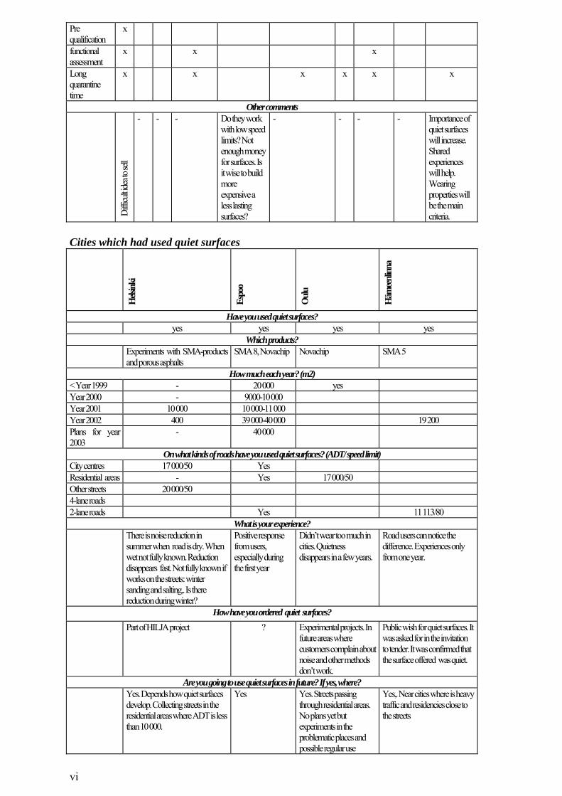
vi

Pre qualification

x

functional assessment

x x x

Long quarantine time

x x x x x x

Other comments

Diffic

ult id

ea to

sell

- - - Do they work with low speed limits? Not enough money for surfaces. Is it wise to build more expensive a less lasting surfaces?

- - - - Importance of quiet surfaces will increase. Shared experiences will help. Wearing properties will be the main criteria.

Cities which had used quiet surfaces

Hels

inki

Espo

o

Oulu

Häm

eenli

nna

Have you used quiet surfaces? yes yes yes yes

Which products? Experiments with SMA-products

and porous asphalts SMA 8, Novachip Novachip SMA 5

How much each year? (m2) < Year 1999 - 20 000 yes Year 2000 - 9000-10 000 Year 2001 10 000 10 000-11 000 Year 2002 400 39 000-40 000 19 200 Plans for year 2003

- 40 000

On what kinds of roads have you used quiet surfaces? (ADT/ speed limit) City centres 17 000/50 Yes Residential areas - Yes 17 000/50 Other streets 20 000/50 4-lane roads 2-lane roads Yes 11 113/80

What is your experience? There is noise reduction in

summer when road is dry. When wet not fully known. Reduction disappears fast. Not fully known if works on the streets: winter sanding and salting,. Is there reduction during winter?

Positive response from users, especially during the first year

Didn’t wear too much in cities. Quietness disappears in a few years.

Road users can notice the difference. Experiences only from one year.

How have you ordered quiet surfaces? Part of HILJA project ? Experimental projects. In

future areas where customers complain about noise and other methods don’t work.

Public wish for quiet surfaces. It was asked for in the invitation to tender. It was confirmed that the surface offered was quiet.

Are you going to use quiet surfaces in future? If yes, where? Yes. Depends how quiet surfaces

develop. Collecting streets in the residential areas where ADT is less than 10 000.

Yes Yes. Streets passing through residential areas. No plans yet but experiments in the problematic places and possible regular use

Yes,. Near cities where is heavy traffic and residencies close to the streets

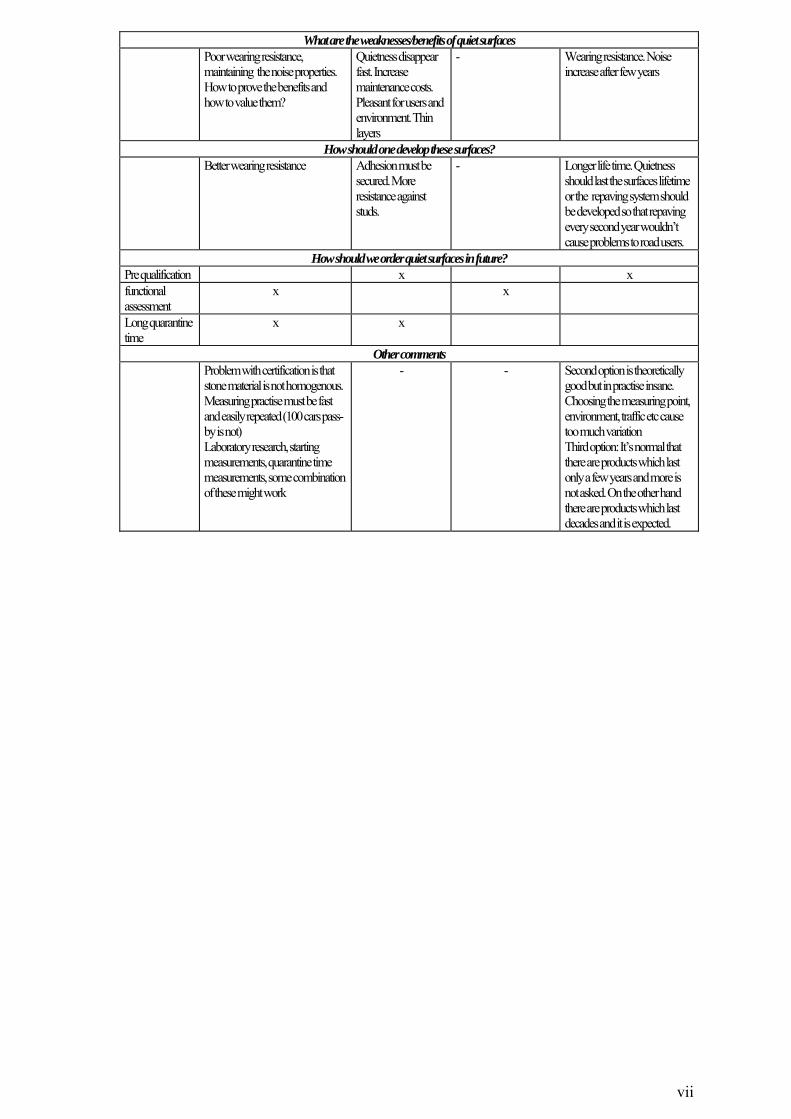
vii

What are the weaknesses/benefits of quiet surfaces Poor wearing resistance,

maintaining the noise properties. How to prove the benefits and how to value them?

Quietness disappear fast. Increase maintenance costs. Pleasant for users and environment. Thin layers

- Wearing resistance. Noise increase after few years

How should one develop these surfaces? Better wearing resistance Adhesion must be

secured. More resistance against studs.

- Longer life time. Quietness should last the surfaces lifetime or the repaving system should be developed so that repaving every second year wouldn’t cause problems to road users.

How should we order quiet surfaces in future? Pre qualification x x functional assessment

x x

Long quarantine time

x x

Other comments Problem with certification is that

stone material is not homogenous. Measuring practise must be fast and easily repeated (100 cars pass-by is not) Laboratory research, starting measurements, quarantine time measurements, some combination of these might work

- - Second option is theoretically good but in practise insane. Choosing the measuring point, environment, traffic etc cause too much variation Third option: It’s normal that there are products which last only a few years and more is not asked. On the other hand there are products which last decades and it is expected.

ISBN 951-22-7693-3ISBN 951-22-7694-1 (PDF)ISSN 1795-2239ISSN 1795-4584 (PDF)