1

Measuring the Hubble Constant

Yick Chee Fong

Supervised by Dr Carlo Contaldi

Theoretical Physics

Blackett Laboratory

Imperial College London

London SW7 2AZ

United Kingdom

Submitted in partial fulfillment of the requirements for the degree of

Master of Science of Imperial College London

23 September 2011

2

Abstract

The Hubble constant is an important cosmological parameter that describes the expansion

rate of the universe. While it is not regarded as a fundamental parameter in standard cosmological

models, it can be measured by various independent methods and enables us to exploit the wealth of

observational data to advance our theoretical understanding in cosmology. We first review the

motivations for measuring the Hubble constant. We discuss how independent Hubble constant

measurements can break the geometrical degeneracy in cosmic microwave background

measurements so that one can precisely determine the spatial curvature and dark energy densities.

We also discuss how independent Hubble constant measurements can improve the constraints on

cosmological parameters derived from cosmic microwave background measurements, specifically

the equation of state for dark energy and the neutrino mass. Furthermore, we discuss the

application of the Hubble constant to predict the age of the universe, which can be compared

against independent estimates from stellar chronometry on the oldest stars and cosmic microwave

background measurements so as to validate our understanding on the underlying cosmology of the

universe. We then review various modern methods to measure the Hubble constant, focusing on

their underlying physics, major sources of systematic errors and recent results. Based on the Hubble

law, various distance methods have been devised to determine the Hubble constant via distance

measurements on different types of galactic objects. Among these, we discuss the currently most

powerful methods using Cepheids, type Ia supernovae, the tip of red giant branch, the Tully-Fisher

relation and surface brightness fluctuations, as well as a promising method using masers. Other

complementary, and potentially competitive, non-distance methods have been developed: we

discuss the methods based on baryon acoustic oscillations, Sunyaev-Zel’dovich effect, gravitational

lens time delays and gravitational waves. At present, the Hubble constant values predicted by

various methods span a wide range from low 60s to high 70s (km per second per mega-parsec), and

a more thorough physical understanding on the systematics affecting each method may be required

for the predicted values to converge. We suggest a reasonable and safe approach of adopting a

value derived from a combination of independent high quality measurements: a good set comprises

cosmic microwave background, Cepheid, type Ia supernova and baryon acoustic oscillations

measurements and gives the Hubble constant as km s-1 Mpc-1 (Komatsu et al. 2011).

Finally, we highlight the future developments in observational cosmology which are expected to

improve the accuracies of the various methods discussed to the 1-3% level.

3

Contents

1. Introduction 6

2. Motivations for Measuring the Hubble Constant 13

2.1 Physical Origins of CMB Anisotropies 13

2.2 Geometrical Degeneracy 16

2.3 Constraining the Equation of State for Dark Energy 18

2.4 Constraining the Neutrino Mass 21

2.5 Age of the Universe 23

3. Distance Methods to Measure the Hubble Constant 25

3.1 Cepheids 25

3.1.1 Physical Origin 25

3.1.2 Observational Properties – the Leavitt Law 26

3.1.3 Fundamental Techniques to Calibrate Cepheid Distances 28

3.1.4 Main Sources of Systematic Errors 30

3.2 Type Ia Supernovae 32

3.2.1 Observational Properties 32

3.2.2 Underlying Physics 35

3.3 Recent Results for the Hubble Constant by Cepheid and Type Ia

Supernova Distances

36

3.4 Tip of the Red Giant Branch Method 38

3.5 Tully-Fisher Method 40

3.6 Surface Brightness Fluctuations Method 42

3.7 Masers 43

3.8 Hubble Diagram based on Modern Distance Measurements 45

4

4. Other Methods to Measure the Hubble Constant 48

4.1 Baryon Acoustic Oscillations 48

4.1.1 Physical Relation to the Hubble Constant 48

4.1.2 Error Sources 50

4.1.3 Recent Results for the Hubble Constant using BAO measurements 53

4.2 Sunyaev-Zel’dovich Effect 54

4.2.1 Inverse-Compton Scattering 55

4.2.2 Thermal SZE 58

4.2.3 Other Types of SZE: Non-thermal, Kinematic and Polarization 59

4.2.4 Method of Measuring the Hubble Constant via the SZE 61

4.2.5 Major Systematics 63

4.2.6 Recent Results for the Hubble Constant Measured via the SZE 66

4.3 Gravitational Lens Time Delays 66

4.3.1 Fundamental Principles 66

4.3.2 Constraints, Degeneracies and Other Difficulties 69

4.3.3 Recent Results for the Hubble Constant 72

4.4 Gravitational Waves 73

5. Conclusion 75

Acknowledgements 77

Reference 78

5

List of Figures

1.1 The original Hubble diagram 7

2.1 Schematic representation of the CMB power spectrum for scale invariant adiabatic

scalar models

14

2.2 Degeneracy lines in the plane for a fixed 17

2.3 Likelihood ratio contours in the plane for models containing only scalar

modes

18

2.4 Projected accuracies for the equation of state for dark energy due to improved

CMB and Hubble constant measurements

20

2.5 Improved constraint on the total mass of neutrinos due to independent Hubble

constant measurements via baryon acoustic oscillations and supernovae

22

3.1 The Cepheid manifold 28

3.2 Spectra of normal type Ia supernovae 33

3.3 Light curves of SN 1992A observed at three wavelengths 34

3.4 Red giant branch luminosity function of NGC 5253 39

3.5 Tully-Fisher relations at various wavelengths for galaxies calibrated with

independent Cepheid measurements from the Hubble Space Telescope Key Project

41

3.6 Prototype H2O maser galaxy NGC 4258 44

3.7 Hubble diagram based on modern distance measurements 46

4.1 Schematic diagram for the Alcock-Paczynski test 49

4.2 Schematic illustration of the correlation function and the power spectrum for

baryon acoustic oscillations

50

4.3 Peak broadening in the correlation function and damping in the power spectrum

due to non-linear clustering

53

4.4 Schematic galaxy distributions showing the effects due to peak broadening in the

correlation function and damping in the power spectrum

53

4.5 Sunyaev Zel’dovich effect (SZE) of a fictional cluster 1000 times more massive than

a typical cluster

54

4.6 The spectral deformation caused by inverse-Compton scattering of an incident

Planck spectrum after a single scattering from a thermal population of electrons as

a function of dimensionless frequency

57

4.7 Relative strengths of the thermal and kinematic Sunyaev Zel’dovich effects (SZE) 61

4.8 Basic ray geometry of gravitational lensing 67

6

1. Introduction

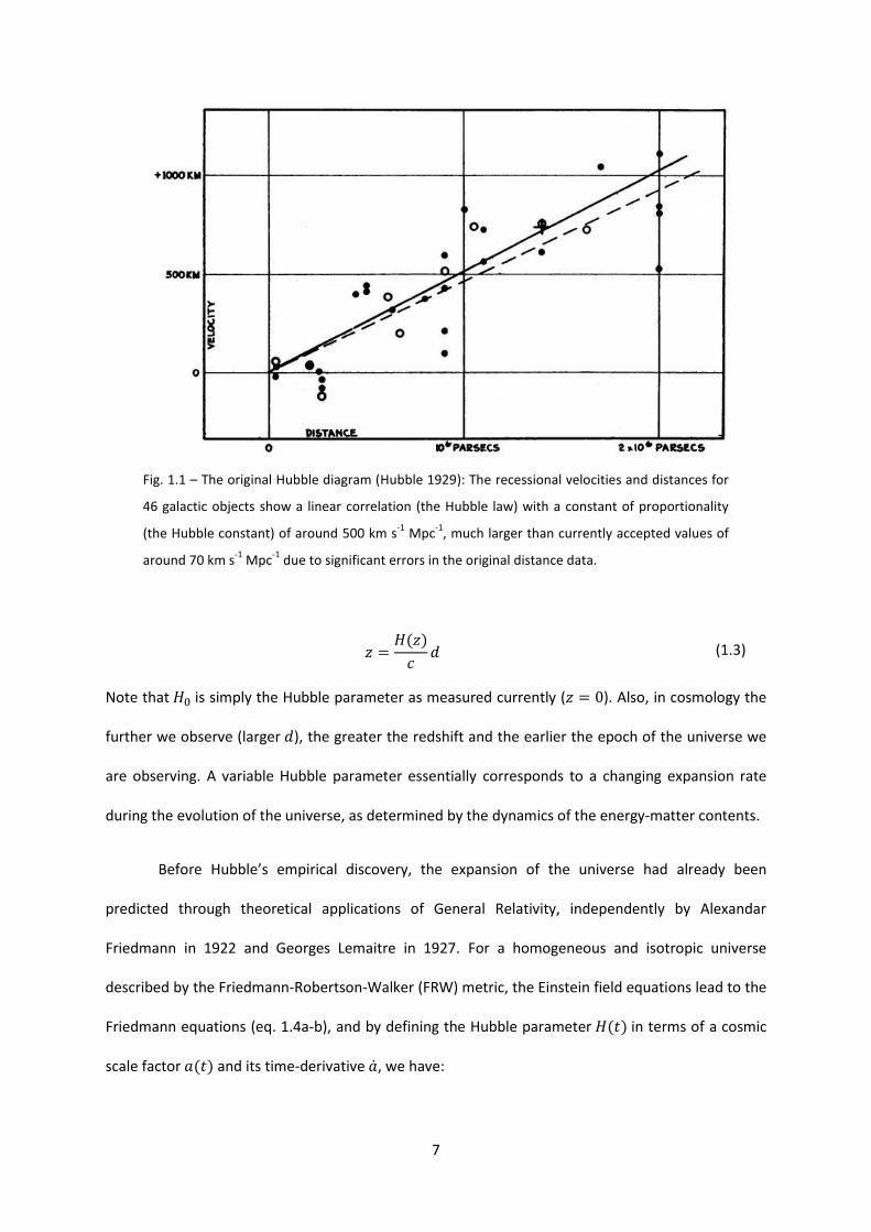
In 1929, Edwin Hubble discovered a linear correlation between the distance ( ) and

recessional velocity ( ) measurements of galaxies as far as the Virgo cluster (see Fig. 1.1 for the

original Hubble diagram):

(1.1)

This empirical relation (referred as the Hubble law) suggests that the more distant a galaxy is from us,

the faster it moves away from us. It provided the first piece of direct evidence for the expansion of

our universe (where spacetime itself is expanding) and prompted Einstein to abandon his attempts

to build a static universe model via the cosmological constant (which, however, would be re-

introduced later due to the inferred existence of dark energy). The proportionality factor ( ) in this

relation became to be known as the Hubble constant, and is a measure of the current expansion rate

of the universe. Its value as originally determined by Hubble (500 km s-1 Mpc-1) was almost an order

of magnitude larger than currently accepted values (around 70 km s-1 Mpc-1), due to significant

errors in the original distance measurements available to Hubble (Tammann 2005). Note that the

Hubble constant is often expressed numerically as , equal to divided by 100 km s-1 Mpc-1; for

example, in the above km s-1 Mpc-1 is equivalent to .

In practice, the recessional velocity can be determined accurately from the redshift ( ) of the

galaxy ( and below refer to observed and emitted wavelengths respectively):

(1.2)

For small redshifts ( ), and the Hubble law (eq. 1.1) can be expressed as .

However, for larger redshifts the relation between the recessional velocity and redshift is non-linear

and dependent on the cosmology (i.e. energy-matter contents) of the universe. The Hubble law can

then be re-expressed, using the Hubble parameter , as:

7

Fig. 1.1 – The original Hubble diagram (Hubble 1929): The recessional velocities and distances for

46 galactic objects show a linear correlation (the Hubble law) with a constant of proportionality

(the Hubble constant) of around 500 km s-1

Mpc-1

, much larger than currently accepted values of

around 70 km s-1

Mpc-1

due to significant errors in the original distance data.

(1.3)

Note that is simply the Hubble parameter as measured currently ( ). Also, in cosmology the

further we observe (larger ), the greater the redshift and the earlier the epoch of the universe we

are observing. A variable Hubble parameter essentially corresponds to a changing expansion rate

during the evolution of the universe, as determined by the dynamics of the energy-matter contents.

Before Hubble’s empirical discovery, the expansion of the universe had already been

predicted through theoretical applications of General Relativity, independently by Alexandar

Friedmann in 1922 and Georges Lemaitre in 1927. For a homogeneous and isotropic universe

described by the Friedmann-Robertson-Walker (FRW) metric, the Einstein field equations lead to the

Friedmann equations (eq. 1.4a-b), and by defining the Hubble parameter in terms of a cosmic

scale factor and its time-derivative , we have:

8

(1.4a)

(1.4b)

The cosmic scale factor describes the relative size of the universe ( at present and at the

Big Bang), thereby allowing the interpretation of the Hubble parameter as the expansion

rate. and refer to the density and pressure of individual energy-matter components labeled by

the subscript , each with its distinct equation of state reflecting its nature and

properties. specifies the global spatial geometry of the universe (+1, 0, –1 for open, flat and closed

geometries respectively).

Often the densities are expressed in units of the critical density (the total

energy-matter density below which an expanding universe without dark energy would eventually re-

collapse) as , so that eq. (1.4a) can be re-written as

(1.4c)

where we have used the monotonic relationship between cosmic time and redshift of the FRW

universe to re-parameterize in , while the spatial geometry of the universe has been expressed as

the curvature density (with ). The subscript 0 indicates that the value is

taken at present. In general, we also have . Current observations are

consistent with the standard concordance (ΛCDM) model with (matter consisting of a

small fraction of baryons and mostly cold dark matter), (dark energy in the form of a

cosmological constant, ) and (spatially flat). For details on the cosmological context,

the reader may refer to standard texts such as Dodelson (2003).

The above theoretical relations (eq. 1.4a-c) describe how the energy-matter contents and

the geometry of the universe govern the evolution of the expansion rate. Crucially, they suggest that

information on the Hubble parameter, obtained by direct or indirect measurements, may help us

9

infer and better understand the underlying cosmology of the universe. Specifically, while high quality

measurements on the CMB anisotropies have enabled us to determine various cosmological

parameters with high precisions and accuracies, there exists a nearly exact geometrical degeneracy

that permits cosmological models with different values for and to agree with the same CMB

anisotropies. Thus, it is fundamentally impossible to determine the spatial curvature of the universe

solely from CMB measurements. To break this geometrical degeneracy, one can incorporate

independent measurements on the Hubble constant ( ) in the analysis of CMB measurements to

obtain constraints on and . Furthermore, independent measurements of high accuracies

can complement CMB measurements to derive tighter constraints on other cosmological parameters

such as the equation of state for dark energy (where it is no longer assumed to be a cosmological

constant) and the neutrino mass. Another interesting application of measurements is the

determination of the age of the universe, which depends on the underlying cosmology as well as the

expansion rate. Theoretical estimates based on and an assumed cosmological model can be

compared against estimates from independent methods using stellar chronometry and CMB

measurements. Historically, the inconsistency between the predicted ages based on matter-

dominated models without dark energy (for any values greater than 50 km s-1 Mpc-1) and stellar

chronometry applied to the oldest stars in the Milky Way had provided strong indication for the

existence of dark energy. These topics will be discussed further in Section 2 to provide some

motivations for measuring the Hubble constant.

Most of the historical and modern observations to determine the Hubble constant employ

one or a combination of distance measurement methods. As the recessional velocity of a galaxy can

be accurately measured from the observed redshift, one can determine the Hubble constant (via the

Hubble law) essentially by measuring the distance to the galaxy. One can measure the angular

diameter distance or the luminosity distance , based on the simple facts that the more distant

an object is, the smaller and fainter it will appear to the observer. Quantitatively,

10

(1.5a)

(1.5b)

where are the proper size, apparent angular size (in radians), intrinsic luminosity and

observed flux (integrated over all wavelengths) respectively. They measure the true distance and are

related by . The relations above (eq. 1.5a-b) allow one to determine the relative

distance of the observed object. To determine directly the absolute distance, the intrinsic size or

luminosity of the observed object must be known – astrophysical objects as such are known as

‘standard rulers’ and ‘standard candles’ respectively. Various types of standard candles, such as

Cepheids and type Ia supernovae, exist in sufficient numbers across the universe from our own

galaxy to very distant galaxies. In addition, the absolute distance can be measured, using

trigonometric parallax, directly and accurately for objects very close or within our galaxy (less than 1

kpc away). Astrophysical objects for which we can directly determine the absolute distance are

primary distance indicators, while those that we have to calibrate, via the relative distance relations

eq. (1.5a-b), using known distances of primary indicators (located in the same galaxy hosts) are

known as secondary distance indicators. With astronomical observations accumulated over years,

one can construct a cosmic distance ladder, which is a succession of partially overlapping patches of

distance scales calibrated using various methods, to obtain the distances of nearby to very distant

galaxies (for a detailed review on galactic distance measurements, see Rowan-Robinson 1985).

Despite the seemingly simple underlying concept for the distance methods to determine the

Hubble constant, there exist sources of systematic errors that can severely affect the calibration of

the distance scales. Corrections for these errors are not straightforward especially where the

underlying physics is not well understood. Even if the same observational data is used, different

approaches to correct for possible systematics may result in widely inconsistent estimates of the

Hubble constant (as much as more than 15% difference). Nevertheless, distance measurement

methods continue to play a key role in Hubble constant measurements due to their advantages: the

relatively large number of observed galaxies where the methods can be applied; the availability of

11

well established empirical calibration techniques in spite of imperfect theoretical understanding; and

the good consistency, in general, of their predictions with results obtained by other independent

methods (Section 4). In Section 3 we review the main modern distance methods: the uses of

Cepheids, type Ia supernovae, tip of the red giant branch and masers, as well as the Tully-Fisher and

surface brightness fluctuations methods. We focus on the underlying physics that enables the

distance measurement as well as the major systematics, and also highlight some recent results for

the Hubble constant as determined by these methods.

While the distance methods are empirically effective for the purpose of estimating the

Hubble constant, our theoretical understanding on the distance indicators is far from thorough,

rendering it difficult to ascertain the reliability of our calibration and error correction procedures in

using these distance indicators. Thus, we need other independent methods, ideally based on well

established physics, to provide alternative estimates of the Hubble constant so as to, hopefully,

confirm the validity of the results by a consistency check. As mentioned earlier, CMB anisotropies,

which are theoretically well understood, can be analyzed in conjunction with other independent

measurements (primarily to break the geometrical degeneracy) to derive a tight constraint on the

Hubble constant amongst constraints on other parameters. In addition, baryon acoustic oscillations

(BAO), which arise from the same process that produces the CMB radiation, provide a standard ruler

in the form of a characteristic length scale in the underlying matter distribution. Information on the

Hubble parameter is contained the radial mode of this characteristic length scale at different

redshifts, and hence we can derive the Hubble constant from BAO measurements. Another

independent method uses measurements of the Sunyaev-Zel’dovich effect (SZE) and the X-ray

emission due to galaxy clusters. This method crucially makes use of the different dependences on

electron density along the same path-length in the electron gas, to estimate the angular size and

therefore the angular diameter distance of the galaxy cluster. The Hubble constant can then be

obtained by combining this information with the measured redshift. Furthermore, gravitational

lensing can produce, from the same source, multiple images that have different propagation times

12

to us. If the source luminosity varies in a regular manner, the relative time delays, which are

inversely proportional to the Hubble constant and dependent on the lens mass distribution, can be

used to derive the value of the Hubble constant. Lastly, gravitational waves from coalescing binary

systems provide a plausible means to determine the Hubble constant that is completely

independent of electromagnetic observations used in all of the previously mentioned methods. We

review these methods in Section 4.

Finally, in Section 5 we summarize the current outlook on the subject of Hubble constant

measurements; in particular, we briefly highlight some key on-going and future projects to obtain

improved measurements on the Hubble constant.

13

2. Motivations for Measuring the Hubble Constant

In this section we first review how accurate independent Hubble constant measurements

can be used in the analysis of high quality cosmic microwave background (CMB) data to improve

constraints on key cosmological parameters. We briefly recap the physical origins of CMB

anisotropies (Section 2.1), highlighting how their features are related to the underlying cosmological

parameters, and then discuss the applications of Hubble constant measurements to break the

geometrical degeneracy (Section 2.2) as well as to derive better constraints on the equation of state

for dark energy (Section 2.3) and the neutrino mass (Section 2.4). We also discuss the implications of

the Hubble constant on the predicted age of the universe (Section 2.5).

2.1 Physical Origins of CMB Anisotropies

The CMB is essentially formed by primordial photons that were released after recombination

(at approximately 3 × 105 years after Big Bang, corresponding to a redshift ) and since then

have been largely free-streaming. While the CMB spectrum, i.e. its intensity as a function of

frequency and direction on the sky, is an extremely good blackbody with a nearly uniform

temperature in all directions (Fixsen et al. 1996), anisotropies exist. The underlying physical

mechanisms can be understood using linear perturbation theory, where anisotropies are generally

described in terms of temperature fluctuation and polarization (the latter is a higher order effect).

Prior to recombination, photons and baryons were tightly coupled due to Thomson and

Coulomb scattering. Initial density fluctuations in this photon-baryon fluid led to pressure gradients

which, together with competing gravitational forces, produced acoustic oscillations. Shortly after

recombination, photon-baryon decoupling occurred as the scattering rates became slower than the

accelerating rate of expansion of the universe. Thus, the CMB spectrum observed today captures the

acoustic oscillations pattern as imprinted on the CMB photons at decoupling. Fig. 2.1 shows a

schematic representation of the CMB spectrum for scale invariant adiabatic scalar models.

14

Fig. 2.1 – Schematic representation of the CMB power spectrum for scale invariant adiabatic scalar

models (Hu et al. 1997): This figure illustrates the various contributions to the overall CMB

spectrum (black solid curve ‘Total’) as discussed in Section 2.1. Note that ‘Effective Temp’ includes

the ‘Redshift’ contribution. Features in open models would be shifted to significantly smaller

angles compared with Λ and models, represented here as a shift in the axis beginning at

the quadrupole . The arrows show the dependence of each contribution on the cosmology.

For instance, a decrease in (subscript 0 in this figure refers to cold dark matter, for which we

use subscript m), corresponding to an increase in radiation content, enhances the ‘Early ISW’ and

thus broadens the first peak; furthermore it also impacts the peak heights via its effects on the

‘Effective Temp’. An increase in will enhance the odd peaks relative to the even peaks via the

‘Effective Temp’ and ‘Acoustic Velocity’ contributions. Similarly, other parameters affect the

profile of the CMB spectrum via various contributions (for details, refer to references within

Section 2.1). Note that in the figure above is the ionization fraction.

In Fig. 2.1, ‘Effective temperature’ refers to the anisotropies attributed to the Sachs-Wolfe

effect, due to acoustic oscillations of the photon-baryon fluid and gravitational redshifts of the

photons as they decouple from baryons and stream out of potential wells (the latter contribution is

15

shown by the ‘redshift’ curve). The Sachs-Wolfe effect depends on the initial conditions of the

universe and the sound horizon , where is the conformal time at recombination and is the

speed of sound, which depends crucially on the baryon-photon density ratio as follows:

(2.1)

Meanwhile, the velocity profile associated with the acoustic oscillations of the photon-baryon fluid

also contributes to the anisotropies (the ‘acoustic velocity’ curve) via Doppler effect. However, this

contribution is small, though measurable, relative to that of the Sachs-Wolfe effect as it is

suppressed by the presence of even a tiny amount of baryons. Furthermore, there are contributions

from the integrated Sache-Wolfe (ISW) effect, which is caused by time-variations in the gravitational

potential and acts on the photons during their free-streaming from the last scattering surface to us.

‘Early ISW’ occurs before the matter domination phase of the expanding universe (after last

scattering) while ‘late ISW’ occurs after curvature or dark energy domination, and their contributions

to the CMB spectrum depend respectively on (early ISW) and or (late ISW). Lastly,

‘diffusion cutoff’ is a damping effect due to imperfect coupling between photons and baryons.

Photons diffuse over a length scale approximately proportional to

and smoothen

out the anisotropies. This corresponds to the washing out of small scale (large ) features in Fig. 2.1.

Overall, the detailed profile of the CMB spectrum, such as the positions of its peaks and troughs, the

spacing between adjacent peaks and the locations of the peaks, is determined by (in decreasing

order of importance) the initial conditions and the contents of the universe before and after

recombination (via effects on various contributions as indicated in Fig. 2.1). As such, precise CMB

measurements allow us to derive tight constraints on four fundamental parameters (Hu & Dodelson

2002): the physical dark matter density ( ), the physical baryon density (

), the comoving

angular diameter distance between recombination and present ( ) and the overall spectral tilt ( )

(Fig. 2.1 assumes ). Note that the third parameter contains information on curvature ( ) or

16

dark energy ( ), while the fourth relates to the initial conditions. From these, other secondary

parameters, including the Hubble constant km s-1 Mpc-1), may be derived. For details on

the physics of CMB anisotropies, see e.g. Hu et al. (1997), Hu & Dodelson (2002) and Dodelson (2003)

(the first two for a more qualitative overview and the third for a more quantitative discussion).

2.2 Geometrical Degeneracy

Various degeneracies among cosmological parameters exist in the CMB anisotropies

(Efstathiou & Bond 1999). These parameter degeneracies span a wide range over the sensitivity to

CMB measurements, but most are, in principle, breakable if sufficiently precise measurements are

available. However, there is a nearly exact geometrical degeneracy such that CMB anisotropies alone,

when analyzed using linear perturbation theory, cannot distinguish models with different

background geometries but identical (non-dark energy) matter contents regardless of the precision

of the CMB measurements. Thus, this geometrical degeneracy imposes fundamental limits on how

well one can determine the curvature of the universe as well as the Hubble constant from CMB

anisotropies alone.

We recall from Section 2.1 that cosmological parameters describing the energy-matter

contents of the universe, i.e. physical densities ( ) of baryons, cold dark matter, curvature

and dark energy, have measurable effects on the CMB spectrum. Clearly, recalling

from Section 1, the physical densities obey the following constraint equation:

(2.2)

Physically, these parameters influence the CMB spectrum via two physical scales, the sound horizon

at recombination and the angular diameter distance to the last scattering surface. The former

depends on baryon and dark matter physical densities but not curvature or dark energy (since the

latter two are dynamically negligible at recombination). The latter depends on the combined

physical density of baryons and dark matter, as well as the physical densities of curvature and dark

17

energy. The mapping from these parameters to the CMB spectrum is such that models with different

combinations of curvature and dark energy lead to indistinguishable features at high multipoles of

the spectrum, and hence the geometrical degeneracy. This is illustrated by the degeneracy lines in

Fig. 2.2. As illustrated by Fig. 2.3, a greater precision in CMB measurements merely corresponds to

narrowing around the degeneracy line without being able to rule out certain combinations of

curvature and dark energy. Thus, the geometrical degeneracy is fundamental, in the sense that it

cannot be broken by improving CMB observations alone. Note that at low multipoles curvature and

dark energy do result in distinguishable CMB features, but these differences are less significant than

the errors due to cosmic variance (i.e. limited sample size for large-scale measurements in a finite

universe), hence it is impossible to break the geometrical degeneracy from CMB anisotropies alone.

Fig. 2.2 – Degeneracy lines in the plane for a fixed (Efstathiou & Bond 1999): Each

degeneracy line is labeled by a parameter that depends on various component densities, and

represents the curvature and dark energy densities that would give rise to the same observed

CMB anisotropies given fixed total matter density ( ) and primordial fluctuation spectrum.

The five dots indicate models for which the baryon and cold dark matter densities ( and )

are, in fact, individually identical (i.e. not just their sum which is fixed along each degeneracy line);

despite their different curvature and dark energy densities, their CMB anisotropies would be

undistinguishable, illustrating the geometrical degeneracy.

18

The constraint equation (eq. 2.2) implies that one may use independent constraints on the

Hubble constant (or dark energy), obtained from measurements other than the CMB spectrum, to

break the geometrical degeneracy. In particular, when the matter content parameters are well

constrained by CMB measurements, a constraint on the Hubble constant directly converts into a

constraint on dark energy. In general, . An accuracy of for can be

achieved if the errors on can be kept to 5% (Efstathiou & Bond 1999).

Fig. 2.3 – Likelihood ratio contours in the (physical densities) plane for models containing

only scalar modes (Efstathiou & Bond 1999): Similarly as Fig. 2.2, the solid curve is a degeneracy

line with a fixed parameter , and all models have identical baryon and cold dark matter densities

( and ). The (approximate) , and contours are generated from actual (but older)

observational data (refer to the original paper for details). Improved observational sensitivities

would allow one to zoom into contours of higher likelihood, but these regions still lie along the

degeneracy line and hence the geometrical degeneracy cannot be broken in this way.

2.3 Constraining the Equation of State for Dark Energy

Besides the cosmological constant ( ), other candidates for dark energy have been

proposed, e.g. cosmic strings ( ), domain walls ( ), quintessence (constant

or dynamical w). CMB measurements, when combined with other independent

19

cosmological measurements, provide direct constraints on the dark energy equation of state. In fact,

Hu (2005) suggests that an independent Hubble constant measurement accurate to the percent

level is the single most useful complement to CMB parameters for dark energy studies. This appears

counter-intuitive because the Hubble constant is measured at present while the CMB is primarily a

snapshot of the last scattering surface where dark energy was subdominant. The essence of how this

works is that CMB anisotropies provide two self-calibrated (internally consistent) standards for dark

energy studies: the sound horizon at recombination and the initial amplitude of fluctuations at the

Mpc-1 scale. With the expansion history in the decelerating phase fixed according to the

standard thermal theory, deviations in the underlying CMB parameters due to the dark energy

equation of state are translated via the two standards into variations in the Hubble constant. With

current calibrations of the two standards using WMAP data alone at an accuracy of ≤4% and ≤10%

respectively, Hu (2005) concludes that a Hubble constant measurement with an accuracy of a few

percent can constrain the dark energy equation of state at a redshift around 0.5 to a comparable

fractional precision (assuming the universe is flat).

A few analytical estimates on the relation between errors in the Hubble constant and dark

energy parameters are provided by Olling (2007). Assuming a flat universe, the current Hubble

constant error of 9.8% contributes roughly half of the uncertainties in the dark energy parameters

(equation of state and density). However, data from the future Planck mission should result in an

eightfold decrease in the other half of the contributions, thus errors in the Hubble constant, if not

reduced significantly, would fully dominate the uncertainties in the dark energy parameters. On the

other hand, significant improvements in the accuracy of the Hubble constant (to 1% level) could

greatly improve the accuracy of the dark energy equation of state (to as good as 2%). Fig. 2.4 shows

the projections by Olling (2007) for future WMAP 8-year and Planck data. Aside, a Hubble constant

measurement with an accuracy at 1% level would decrease the error on the spatial curvature by a

factor 16. In addition, while improvements in the Hubble constant accuracy would eventually offer

20

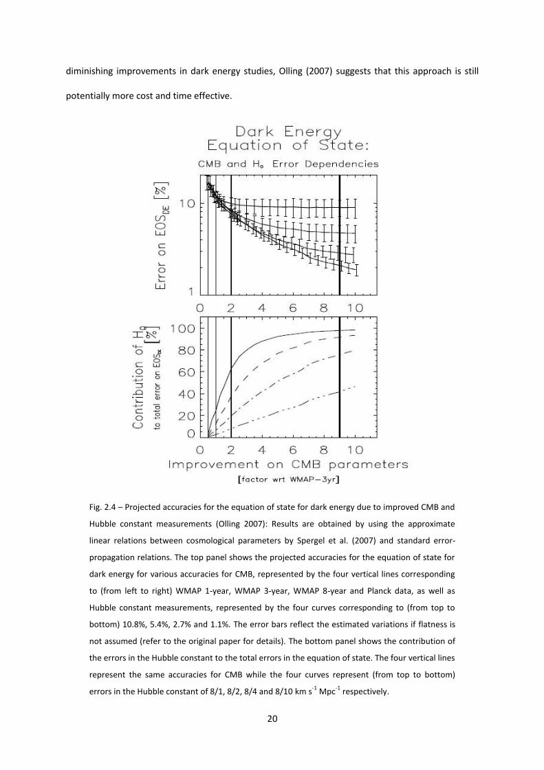
diminishing improvements in dark energy studies, Olling (2007) suggests that this approach is still

potentially more cost and time effective.

Fig. 2.4 – Projected accuracies for the equation of state for dark energy due to improved CMB and

Hubble constant measurements (Olling 2007): Results are obtained by using the approximate

linear relations between cosmological parameters by Spergel et al. (2007) and standard error-

propagation relations. The top panel shows the projected accuracies for the equation of state for

dark energy for various accuracies for CMB, represented by the four vertical lines corresponding

to (from left to right) WMAP 1-year, WMAP 3-year, WMAP 8-year and Planck data, as well as

Hubble constant measurements, represented by the four curves corresponding to (from top to

bottom) 10.8%, 5.4%, 2.7% and 1.1%. The error bars reflect the estimated variations if flatness is

not assumed (refer to the original paper for details). The bottom panel shows the contribution of

the errors in the Hubble constant to the total errors in the equation of state. The four vertical lines

represent the same accuracies for CMB while the four curves represent (from top to bottom)

errors in the Hubble constant of 8/1, 8/2, 8/4 and 8/10 km s-1

Mpc-1

respectively.

21

2.4 Constraining the Neutrino Mass

Despite their abundance in the universe, neutrinos have been difficult to study

experimentally due to their weak interactions. However, neutrino experiments have now established

that neutrinos have non-zero masses and provided constraints on the squared mass differences

between neutrino eigenstates. Furthermore, cosmology has turned out to be a fruitful area for

neutrino studies (see e.g. Crotty et al. 2004 and Hannestad 2006 for detailed reviews). Firstly,

neutrinos contribute to the overall relativistic energy density and play a key role in the evolution of

the universe during the radiation epoch. Neutrino properties affect the time of radiation-matter

equality and the sound horizon at decoupling, and impact mainly on the background (e.g. mean CMB

temperature) evolution. Secondly, neutrino masses determine the extent of their free-streaming and

therefore have implications on the evolution of cosmological fluctuations at the level of background

quantities and directly on the perturbations. Thus, cosmological observations can be used to derive

constraints on neutrino parameters.

An advantage of studying neutrinos through cosmology is that it can provide constraints on

the absolute mass of the neutrinos. Neutrinos affect the CMB spectrum when at least one of the

neutrino masses is greater than the mean energy of relativistic neutrinos per particle at so

that they would be non-relativistic at decoupling. This corresponds to a lower limit on neutrino mass

of eV. If the heaviest neutrino species is lighter than this, then CMB measurements

alone will not reveal any insights into neutrino masses. Supposing that neutrino mass eigenstates are

degenerate with an effective number of species of 3.04 (current standard value), CMB

measurements would be sensitive for total neutrino mass eV (Komatsu et al. 2009). To

probe below this value, one needs additional measurements independent of CMB, such as baryon

acoustic oscillations (BAO) or supernova (SN) data, to place a constraint on the neutrino mass.

The results of Komatsu et al. (2009) illustrate how measurements on the Hubble constant

can improve the constraints on the neutrino mass. Using WMAP 5-year data alone and adopting flat

22

ΛCDM models, they find the constraints on as eV (for ) and eV (for

) respectively (both at 95% confidence level). When BAO and SNe data are added, the

constraints are improved significantly to eV (for ) and eV (for ). This

is due to the additional information on the Hubble constant provided by the BAO and SNe data

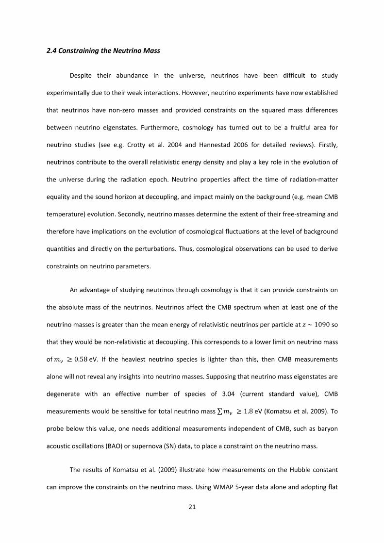
(Ichikawa et al. 2005). Physically, provided that neutrinos are still relativistic during decoupling,

enhances the early ISW effect that causes a shift in the first CMB peak to lower multipoles.

However, as this shift can be countered by a smaller Hubble constant value, there is a degeneracy

(an anti-correlation) between the neutrino mass and the Hubble constant. Thus, independent

Hubble constant measurements can help to break this degeneracy and improve the constraints on

neutrino masses. This is illustrated by Fig. 2.5.

Fig. 2.5 – Improved constraint on the total mass of neutrinos due to independent Hubble constant

measurements via baryon acoustic oscillations and supernovae (Komatsu et al. 2009): The joint

two-dimensional marginalized distributions of and (at 68% and 95 confidence levels) are

shown for the cases where WMAP only and WMAP+BAO+SN results are used respectively. The

much tighter constraint obtained from the latter is largely attributed to the independent distance

information from BAO (to be discussed in Section 4.1).

23

2.5 Age of the Universe

In principle, the age of the universe is determined by the underlying cosmology and the

current expansion rate of the universe (i.e. the Hubble Constant):

(2.3)

In the above the summation is over all energy-matter contents in the universe (including possibly

curvature) in the cosmological model adopted. Eq. (2.3) provides a theoretical prediction based on

the adopted values of the Hubble constant and other cosmological parameters. Alternatively,

observations on stellar evolution or CMB anisotropies, together with their well understood models,

can also be used to estimate the age of the universe. These independent methods should provide

consistent predictions on the age, and by demanding so one may gain insights on the underlying

cosmology as well as the value of the Hubble constant. Historically this has helped provide evidence

or motivation for the existence of dark energy: for a universe without dark energy, any Hubble

constant values greater than km s-1 Mpc-1 resulted in ages that were less than the age estimates

from the observed stellar evolution of the oldest stars in the Milky Way. Based on current commonly

adopted parameters of km s-1 Mpc-1, and , the age of the universe is

estimated to be Gyr (Freedman & Madore 2010).

Observations on the stellar evolution of the oldest stars in globular clusters in our galaxy

allow us to estimate their ages and place a lower limit on the Hubble constant. The age can be

estimated by three independent ways. First is by radioactive dating, where one uses spectroscopic

measurements on the abundance of thorium and uranium (for which the half-lives are known) in

metal-poor stars. Given an initial relative abundance of the two elements from theoretical modeling,

the age can be estimated (for a review, see Sneden et al. 2001). Second is by white dwarf cooling,

which occurs as energy loss from radiation is not replenished since white dwarfs are supported by

electron degeneracy pressure alone. The resulting drop in luminosity, among the faintest white

24

dwarfs, allows one to estimate the age of the galaxy cluster (for a review, see Moehler & Bono 2008).

Third is through modeling the evolution of the temperature-luminosity distribution for a system of

stars. As the stars (of different masses) evolve, their individual temperature-luminosity profiles

change. The temperature-luminosity distribution for the system of stars matches the theoretical

distribution at only one time, thereby allowing one to estimate the age of the stellar system. For this

method, while any stars in the system can be included, main sequence stars have well understood

theoretical models and therefore provide the best age estimates. In particular, the main sequence

turnoff time scale (for the hydrogen supply in the core to be exhausted) can be most robustly

predicted. Using this method (with a separate estimate of the time from the Big Bang to the

formation of the globular clusters), Krauss & Chaboyer (2003) obtains a lower bound of 11.2 Gyr and

a best fit value of 13.4 Gyr (both at 95% confidence level) for the age of the universe. The other two

methods also provide similar estimates for the age of the universe, albeit with larger uncertainties

due to the greater difficulties in modeling the physical processes. Separately, CMB measurements

allow us to derive the Hubble constant and the age of the universe as secondary quantities via the

constraints on and the distance to the last scattering surface by peak heights and positions

respectively. Using WMAP 5-year data with Type Ia SN and BAO data, Komatsu et al. (2009) derives

an age of Gyr. The various methods mentioned have led to consistent predictions on the

age of the universe.

25

3. Distance Methods to Measure the Hubble Constant

In Section 1 we mention that the Hubble constant can essentially be determined via distance

measurements (angular or luminosity) on the receding galaxies due to the relative ease and accuracy

of measuring the recessional velocities via the redshifts. A cosmic distance ladder providing

distances from nearby to distant galaxies can be constructed from the wealth of observational data.

This is crucial for the accurate determination of the Hubble constant, as distance measurements

must be obtained from objects sufficiently far away (at least a few tens of Mpc) so that the

recessional velocities observed are dominated by the Hubble flow (i.e. cosmic expansion) rather than

peculiar motions due to local structures. Furthermore, a large sample used in building the distance

ladder helps to suppress the resulting statistical uncertainties. We also have calibration methods

with high degrees of internal consistency amenable to empirical tests for systematic errors. In

practice, however, various observational and theoretical challenges remain. Few objects are

sufficiently luminous to be well observed at cosmological distances into the Hubble flow. Calibration

techniques for various distance indicators do not always have a solid theoretical basis, thus there

can be severe systematic errors built up in various layers of the distance ladder. Nevertheless, a

number of traditional and modern methods remain effective and promising – Cepheid, type Ia

supernova, tip of giant red branch, maser, Tully-Fisher relation and surface brightness fluctuations.

In the following we discuss the physical origins of these distance indicators, the main underlying

physics as well as sources of systematics, and recent results for these methods.

3.1 Cepheids

3.1.1 Physical Origin

Cepheids provide a widely applicable and powerful means for measuring distances to nearby

galaxies due to the ease of discovering and identifying them and, crucially, the Leavitt law (Leavitt

1908) which is empirically and theoretically well established. Physically, Cepheids arise when

26

massive stars have exhausted the hydrogen in their cores and evolve rapidly back and forth across

the Hertzsprung-Russell (HR) diagram (in the instability strip). The Cepheid has a doubly-ionized

helium layer that acts like a heat engine and valve mechanism. When this ionized layer is opaque to

radiation, energy is trapped and the pressure within increases. As a result, this layer expands and

loses temperature, allowing recombination to occur and therefore causing a decrease in opacity.

More radiation then escapes through the layer and the reverse process occurs. This cycle repeats to

give rise to the observable periodic changes in the Cepheid luminosity (Freedman & Madore 2010;

for details, see Cox 1980).

3.1.2 Observational Properties – the Leavitt Law

The Leavitt law is a relation between the pulsation period, intrinsic luminosity and color. A

simple explanation (following Madore & Freedman 1991 and Rowan-Robinson 1985) is outlined

below. The pulsation period for a Cepheid is related to the natural oscillation period of the star,

which can be shown to be proportional to where is the mean density of the star. As the

natural oscillation period is essentially the time taken for the star to collapse if pressure support

were suddenly removed, one expects:

(3.1)

where is the pulsational constant (which depends on the manner at which pulsation occurs), while

and are the mass and radius of the star respectively. The luminosity of the star is related to its

effective temperature by the Stefan-Boltzmann law:

(3.2)

where is the Stefan-Boltzmann constant. For observational purposes, we describe the luminosity

by the corresponding magnitude or the absolute magnitude (the latter is the magnitude as

observed if the star were at a distance of 10 pc):

27

(3.3a)

(3.3b)

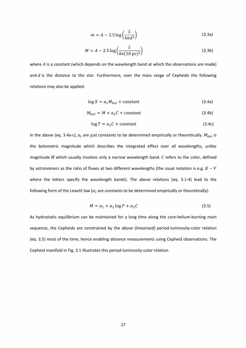
where is a constant (which depends on the wavelength band at which the observations are made)

and is the distance to the star. Furthermore, over the mass range of Cepheids the following

relations may also be applied:

(3.4a)

(3.4b)

(3.4c)

In the above (eq. 3.4a-c), are just constants to be determined empirically or theoretically. is

the bolometric magnitude which describes the integrated effect over all wavelengths, unlike

magnitude which usually involves only a narrow wavelength band. refers to the color, defined

by astronomers as the ratio of fluxes at two different wavelengths (the usual notation is e.g.

where the letters specify the wavelength bands). The above relations (eq. 3.1-4) lead to the

following form of the Leavitt law ( are constants to be determined empirically or theoretically):

(3.5)

As hydrostatic equilibrium can be maintained for a long time along the core-helium-burning main

sequence, the Cepheids are constrained by the above (linearized) period-luminosity-color relation

(eq. 3.5) most of the time, hence enabling distance measurements using Cepheid observations. The

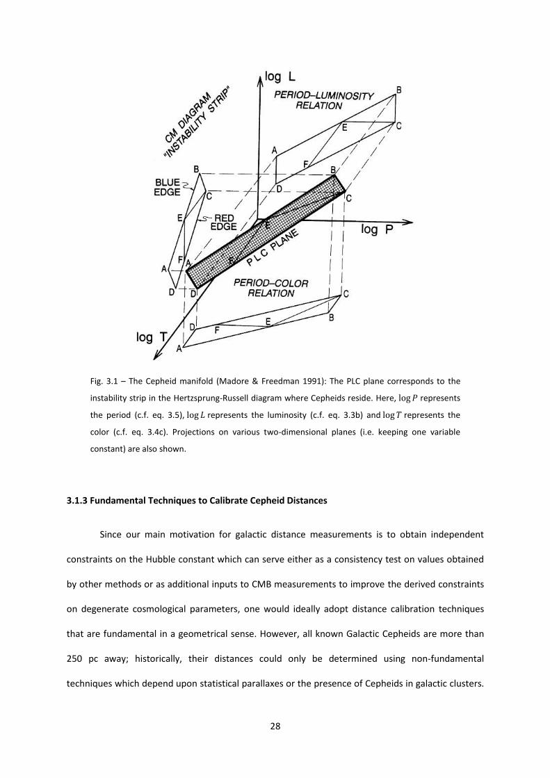
Cepheid manifold in Fig. 3.1 illustrates this period-luminosity-color relation.

28

Fig. 3.1 – The Cepheid manifold (Madore & Freedman 1991): The PLC plane corresponds to the

instability strip in the Hertzsprung-Russell diagram where Cepheids reside. Here, represents

the period (c.f. eq. 3.5), represents the luminosity (c.f. eq. 3.3b) and represents the

color (c.f. eq. 3.4c). Projections on various two-dimensional planes (i.e. keeping one variable

constant) are also shown.

3.1.3 Fundamental Techniques to Calibrate Cepheid Distances

Since our main motivation for galactic distance measurements is to obtain independent

constraints on the Hubble constant which can serve either as a consistency test on values obtained

by other methods or as additional inputs to CMB measurements to improve the derived constraints

on degenerate cosmological parameters, one would ideally adopt distance calibration techniques

that are fundamental in a geometrical sense. However, all known Galactic Cepheids are more than

250 pc away; historically, their distances could only be determined using non-fundamental

techniques which depend upon statistical parallaxes or the presence of Cepheids in galactic clusters.

29

Fortunately, recent progress has led to the development of fundamental techniques that allow us to

calibrate the Cepheid distance-luminosity relation geometrically or quasi-geometrically (the latter

refers to cases where there are non-geometric complications) (Barnes 2009).

Among these, a reliable method for finding Cepheid distances in our galaxy is the infrared

surface brightness method. The Baade-Wesselink method (Baade 1926; Wesselink 1946, 1969)

allows one to determine the mean radius of a Cepheid from its magnitude differences across

multiple phases, given its radial velocity curve. The correlation between the surface brightness and

color, established historically for non-variable stars and recently for Cepheids as well, allows one to

determine the mean surface brightness. Combining these, one can then determine the absolute

surface brightness of the Cepheid. The infrared color index is now commonly used as it is

the most effective in reducing uncertainties. In practice, such color computations require some

interpolation scheme based on accurate period information since V and K photometric data are

seldom collected simultaneously. The equations for finding distance and radius from magnitude,

color and radial velocity can now be solved rigorously and objectively using a Bayesian Markov-Chain

Monte Carlo code due to Barnes et al. (2003).

An alternative is the interferometric pulsation method which uses the observed

interferometric fringe patterns to deduce the angular diameter distance over a pulsation cycle. This

method requires an assumed model for the light distribution of the source, usually a uniform

intensity disk, and a theoretically established limb-darkening curve. Furthermore, it requires a

systematic correction in the form of a p-factor, which accounts for the difference between the

observed radial velocity and the actual pulsation velocity due to effects such as geometrical

projection, limb-darkening, choice of measurement technique, choice of lines measured and spectral

resolution. In fact, this p-factor correction is also needed in the surface brightness method. In this

sense, both methods discussed are quasi-geometric. The interferometric pulsation method does not

use color information and is therefore immune to reddening (discussed in Section 3.1.4). It is also

30

potentially more precise than the surface brightness method, but is limited by the relatively smaller

sample size within the distance where the method can be applied. Nevertheless, it has so far been

useful as a check on the infrared surface brightness distance scale and for finding the p-factor

observationally. Finally, distance measurements of a farther range and a higher precision can be

obtained using trigonometric parallaxes by space missions. Cepheid distances determined by the

previous two techniques agree well with high quality Hubble Space Telescope (HST) data.

3.1.4 Main Sources of Systematic Errors

Error sources in Cepheid distance measurements include statistical (random) errors, which

manifest as the scatter in the period-luminosity relation (observed at a specific color), and various

systematic effects, among which the most significant contributions arise from reddening and

metallicity. Empirically Cepheid data do not follow the ideal (linearized) period-luminosity-color

relation (eq. 3.5), with individual deviations as high as equivalent to a distance error of 30%.

Fortunately, since statistical errors vary inversely with the square root of the sample size, these can

be reduced to 10% with as few as a dozen of Cepheids (Freedman & Madore 2010). Observationally,

the importance of the Magellanic Clouds for the calibration of the cosmic distance ladder is precisely

due to their closeness to us and the large numbers of Cepheids observed in them.

A key source of systematic errors that affect all distance indicators is the reddening effect

(alternatively known as interstellar extinction) which must be corrected before any meaningful

analysis on the observational data can be made. Reddening refers to the wavelength-dependent

absorption and scattering (re-emission) of photons, and it occurs in the parent galaxy of the objects

observed, along the line-of-sight and within our galaxy. It introduces systematic errors into the

derived distances since the observed object will appear fainter and farther than it actually is. If one

collects data at least two wavelength bands (say, V and I) and adopts, as a priori, a value for the ratio

of total-to-selective absorption , then the reddening effect can be incorporated into the constant

in the magnitude relations (eq. 3.3a-b):

31

(3.6)

where is the color excess (defined as the difference between the observed and intrinsic

color indices) obtained from observational data. One can then obtain the Wesenheit magnitude:

(3.7)

which is by construction equivalent to the intrinsic Wesenheit magnitude on the right in eq. (3.7)

(computed using intrinsic values as denoted by subscript 0) and therefore free of reddening. While

this correction technique may break down in regions of intense star formation and extremely high

optical depths, Cepheids are generally sufficiently displaced from such regions for this correction to

be applicable. An alternative technique to minimize reddening is to observe at the longest

wavelengths possible, which is conceptually more robust but practically more challenging.

Besides reddening, another key source of systematic errors is due to the metallicity of the

observed objects. Differences in metal abundance in the stellar chemical compositions affect the

overall stellar structure and the corresponding properties such as color, brightness and radius of the

star. Theoretical studies on how metallicity impacts the period-luminosity relation have so far been

inconclusive. Empirically, two tests of the metallicity-dependence of the period-luminosity relation

have been used for samples in various galaxies. The first test uses measured radial metallicity

gradients within individual galaxies to determine the systematic errors solely due to metallicity. The

second test compares the Cepheid and tip of the red giant branch distance measurements for same

galaxies so as to establish the correlation of these differences with the metallicity. As results are still

being debated, this is very much an active area of research. In practice, as Section 3.3 illustrates

further, significant discrepancies can arise when different correction techniques are applied in the

calibration of distant galactic distances using nearby galactic distances where the galactic

metallicities are largely dissimilar (e.g. majority of the HST Key Project galaxies have metallicities

more comparable to our galaxy than the Large Magellanic Cloud but calibration was done using the

latter). For detailed reviews, see Madore & Freedman (1991) and Freedman & Madore (2010).

32

3.2 Type Ia Supernovae

Type Ia supernovae (SNe Ia) provide the most accurate distance measurements well into the

Hubble flow and is therefore a key distance indicator for measuring the Hubble constant. While our

theoretical understanding on SNe Ia is far from robust, observationally SNe Ia are bright enough to

be observed at great cosmological distances, can be reliably identified and exhibit a correlation of

very low intrinsic scatter between their peak luminosities and rates of decline so that they are good

standard candles. SNe Ia are primary distance indicators in the sense that their distances can be

estimated directly by the Baade-Wesselink method (Baade 1926; Wesselink 1946, 1969). Observing

the time-variation of the supernova luminosity and color, one can deduce the quantity

, where is the radius of the supernova photosphere at time and is the

radius at the instant of maximum luminosity. Using the radial velocity from the measured redshift,

one can then infer the value of . Putting this and the effective supernova temperature inferred

from the observed color into the Stefan-Boltzmann law (eq. 3.2), the maximum intrinsic supernova

luminosity can be determined (Rowan-Robinson 1985). Alternatively, distances of distant SNe Ia are

also calibrated using well measured Cepheid distances in nearby galaxies where both Cepheids and

SNe Ia are observed. In following we discuss the observational properties that make SNe Ia good

standard candles (Section 3.2.1) and our theoretical understanding on SNe Ia (Section 3.2.2).

3.2.1 Observational Properties

SNe Ia can be reliably identified by their spectra, light-curve shapes, colors and magnitudes.

Improved observational data reveal that SNe Ia are not strictly homogeneous, and a readily

distinguishable minority is classified as peculiar SNe Ia. Nevertheless, the majority classified as

normal SNe Ia displays a high degree of homogeneity and remains useful for distance measurements

to determine the Hubble constant.

33

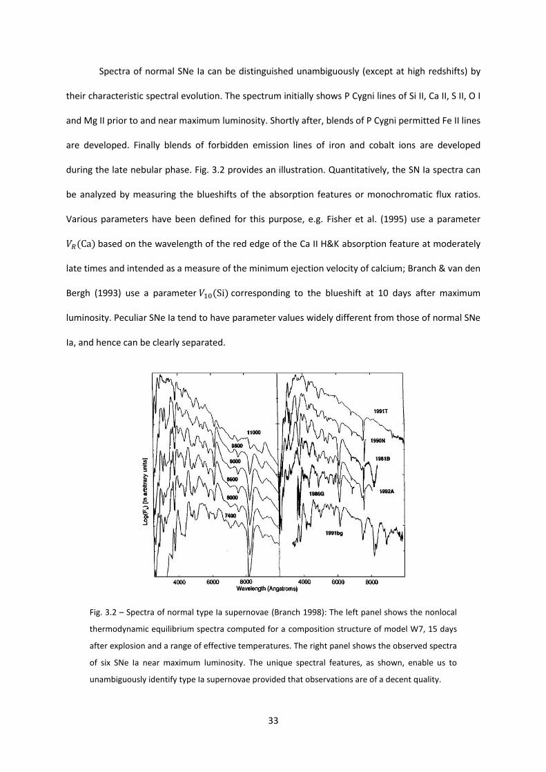
Spectra of normal SNe Ia can be distinguished unambiguously (except at high redshifts) by

their characteristic spectral evolution. The spectrum initially shows P Cygni lines of Si II, Ca II, S II, O I

and Mg II prior to and near maximum luminosity. Shortly after, blends of P Cygni permitted Fe II lines

are developed. Finally blends of forbidden emission lines of iron and cobalt ions are developed

during the late nebular phase. Fig. 3.2 provides an illustration. Quantitatively, the SN Ia spectra can

be analyzed by measuring the blueshifts of the absorption features or monochromatic flux ratios.

Various parameters have been defined for this purpose, e.g. Fisher et al. (1995) use a parameter

based on the wavelength of the red edge of the Ca II H&K absorption feature at moderately

late times and intended as a measure of the minimum ejection velocity of calcium; Branch & van den

Bergh (1993) use a parameter corresponding to the blueshift at 10 days after maximum

luminosity. Peculiar SNe Ia tend to have parameter values widely different from those of normal SNe

Ia, and hence can be clearly separated.

Fig. 3.2 – Spectra of normal type Ia supernovae (Branch 1998): The left panel shows the nonlocal

thermodynamic equilibrium spectra computed for a composition structure of model W7, 15 days

after explosion and a range of effective temperatures. The right panel shows the observed spectra

of six SNe Ia near maximum luminosity. The unique spectral features, as shown, enable us to

unambiguously identify type Ia supernovae provided that observations are of a decent quality.

34

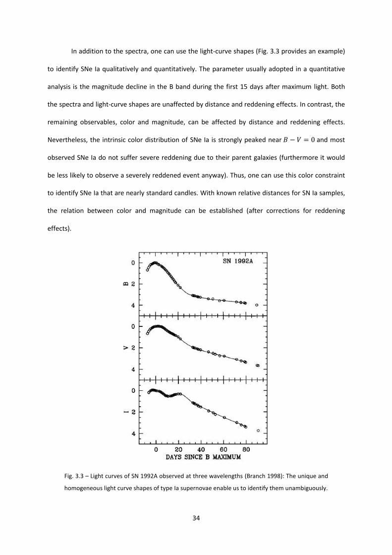
In addition to the spectra, one can use the light-curve shapes (Fig. 3.3 provides an example)

to identify SNe Ia qualitatively and quantitatively. The parameter usually adopted in a quantitative

analysis is the magnitude decline in the B band during the first 15 days after maximum light. Both

the spectra and light-curve shapes are unaffected by distance and reddening effects. In contrast, the

remaining observables, color and magnitude, can be affected by distance and reddening effects.

Nevertheless, the intrinsic color distribution of SNe Ia is strongly peaked near and most

observed SNe Ia do not suffer severe reddening due to their parent galaxies (furthermore it would

be less likely to observe a severely reddened event anyway). Thus, one can use this color constraint

to identify SNe Ia that are nearly standard candles. With known relative distances for SN Ia samples,

the relation between color and magnitude can be established (after corrections for reddening

effects).

Fig. 3.3 – Light curves of SN 1992A observed at three wavelengths (Branch 1998): The unique and

homogeneous light curve shapes of type Ia supernovae enable us to identify them unambiguously.

35

Correlations among the observables mentioned manifest clearly especially when both

normal and peculiar SNe Ia are considered. One can broadly describe SNe Ia as a sequence ranging

from those with high-excitation spectra, high blueshifts of spectral features, slow light curves and

high luminosities to those with low-excitation spectra, low blueshifts, fast light curves and low

luminosities. SNe Ia at the former extreme tend to be seen in blue, late-type galaxies while those at

the latter extreme tend to be seen in red, early-type galaxies. One should also note that within this

broad homogeneity, there exists much diversity in the sense that correlations may not be as strong

as when only normal SNe Ia (which are used as standard candles) are considered. Thus, the strength

of these intrinsic correlations, together with the quality of the calibration of distance-independent

SN Ia observables using, say, nearby Cepheids, will impact on the accuracies of the distance

measurements of SNe Ia and the Hubble constant derived. For a detailed review, see Branch (1998).

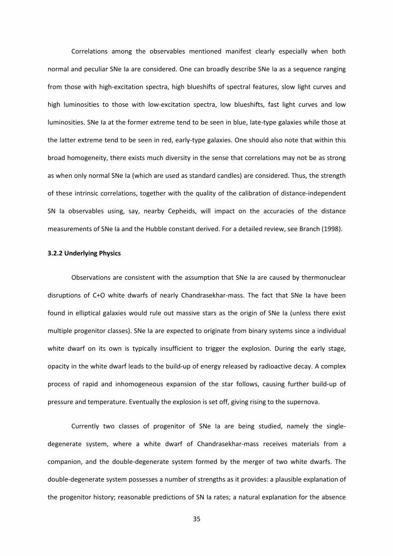
3.2.2 Underlying Physics

Observations are consistent with the assumption that SNe Ia are caused by thermonuclear

disruptions of C+O white dwarfs of nearly Chandrasekhar-mass. The fact that SNe Ia have been

found in elliptical galaxies would rule out massive stars as the origin of SNe Ia (unless there exist

multiple progenitor classes). SNe Ia are expected to originate from binary systems since a individual

white dwarf on its own is typically insufficient to trigger the explosion. During the early stage,

opacity in the white dwarf leads to the build-up of energy released by radioactive decay. A complex

process of rapid and inhomogeneous expansion of the star follows, causing further build-up of

pressure and temperature. Eventually the explosion is set off, giving rising to the supernova.

Currently two classes of progenitor of SNe Ia are being studied, namely the single-

degenerate system, where a white dwarf of Chandrasekhar-mass receives materials from a

companion, and the double-degenerate system formed by the merger of two white dwarfs. The

double-degenerate system possesses a number of strengths as it provides: a plausible explanation of

the progenitor history; reasonable predictions of SN Ia rates; a natural explanation for the absence

36

of H and He in the SN Ia spectra; and a single parameter (total mass) accounting for the SN Ia

sequence. However, for the double-degenerate system to become viable, one must overcome the

critical theoretical challenge of how to avoid its accretion-induced collapse, which is demonstrated

to be highly likely by various numerical studies. Furthermore, few white dwarfs have been observed

so that the double-degenerate system is not expected to account for most SNe Ia. On the other hand,

the single-degenerate system is generally favored since it is consistent with the broad homogeneity

of SNe Ia and at the same time can be fine-tuned to account for the diversities observed. Much

remains to be resolved though, as we have yet to understand the absence of H and He in the

observed spectra (which are expected to be present due to mass transfer from the companion) and

the explosion mechanism. For a detailed review, see Hillebrandt & Niemeyer (2000). Despite the lack

of solid theoretical understanding, SNe Ia are empirically well suited for cosmological distance

measurements needed to determine the Hubble constant.

3.3 Recent Results for the Hubble Constant by Cepheid and Type Ia Supernova Distances

Cepheid and typa Ia supernova distances are often used together to determine the Hubble

constant as they can be calibrated to high accuracies and provide sufficient coverage over the

nearby or far distant (well into Hubble flow) ranges respectively. Tammann et al. (2008) derive

km s-1 Mpc-1 from 29 Cepheids; using 20 Cepheid-calibrated SNe Ia which are close

enough so that no correction is made for CMB dipole motion, they derive km s-1

Mpc-1; and from a separate group of 62 SNe Ia farther out (assuming a flat universe with )

they obtain km s-1 Mpc-1. These independent distance scales, together with other

distance scales studied in their paper (RR Lyrae and tip of the red giant branch) show low dispersion

and derive close values for the Hubble constant. The various distance scales have sufficient overlap

and can be combined into a single distance scale covering nearby to cosmological distances. A

corresponding value for the Hubble constant, given by the unweighted mean from the Cepheids and

Cepheid-calibrated SNe Ia averaged with the TRGB result, is km s-1 Mpc-1. The high

37

consistency of these results may provide confidence in their accuracies. However, Riess et al.

(2009a-b), using measurements of 240 Cepheids from 6 type Ia supernova hosts and one maser

galaxy (Section 3.7), obtain a significantly different value of km s-1 Mpc-1. In a more

recent paper, Riess et al. (2011) attain a best estimate of km s-1 Mpc-1 (total

uncertainty of 3.3%) from data of over 600 Cepheids in 8 recent type Ia supernova hosts. The results

by these authors are highly consistent among themselves as well, but the discrepancy between the

two groups is more than 10% and well beyond the uncertainty allowances.

Tammann et al. (2008) suggest three possible causes for an overestimation of the Hubble

constant by other researchers. They argue that, firstly, an assumption often used in literature, that

the same Cepheid period-luminosity relation can be applied across different galaxies with different

metallicities, is untenable and therefore independent calibrations of period-luminosity relation for

galaxies with different metallicities should be done. Secondly, there exists a selection bias in the

sense that as we observe farther out naturally only the brighter events can be observed. Thus,

distant observations may incorrectly raise the Hubble constant estimate unless one ensures that

necessary corrections are made by checking with a Hubble diagram or incorporating highly accurate

distance measurements (say, from Cepheids, TRGB or RR Lyrae). Finally, they question the reliability

of the Hubble constant estimates which are highly model-dependent.

In contrast, Riess et al. (2009b) argue that the Hubble constant results of Tammann et al.

have been underestimated by due to an inaccurate calibration of Galactic Cepheid

period-luminosity relation, possibly due to the use of obsolete data, errors in the reddening

parameter adopted as well as using a limited sample of long-period Cepheids which would lead to

significant statistical errors. Furthermore, Riess et al. point out that the use of photographic SN Ia

data, which are shown to be unreliable and inconsistent with modern data, would underestimate

the Hubble constant results of Tammann et al. by 2.5%. On the other hand, the calibration of the

absolute distance scale is not seen to be a contributing factor to the differences in the Hubble

38

constant estimates, since the Large Magellanic Cloud distance modulo adopted by both groups are

very close.

Clearly, to improve and converge the Hubble constant estimates by distance methods, we

need, besides better observational data, crucially a better physical understanding of the distance

indicators so as to better correct the systematics inherent in individual data, in particular the

implications on the Cepheid distance calibration due to reddening and metallicity effects to resolve

the above disagreement. An accurate geometrically determined value of the Hubble constant will

have significant impact on cosmology since it can help derive strong constraints on other

cosmological parameters and potentially rule out certain cosmological models. For instance, an

approach by Wiltshire (2007) to explain accelerated expansion without dark energy by an

unexpected failure of the cosmological principle predicts km s-1 Mpc-1 (Leith et al.

2008), and thus would be validated by Tammann et al. (2008) but ruled out by Riess et al. (2009). As

another example, using km s-1 Mpc-1 and WMAP 7-year data, Riess et al. (2011)

obtain the constraints and , which supports a cosmological

constant type of dark energy in our universe and implies an excess of relativistic particle species in

the early universe (from the three known neutrino species) respectively.

3.4 Tip of the Red Giant Branch Method

An independent method useful for comparing against the Cepheid and type Ia supernova

distances discussed is the tip of the red giant branch (TRGB) method. The TRGB method uses the

discontinuity, a sharp decrease, in luminosity observed (see Fig. 3.4 for illustration) when a post-

main-sequence low-mass star transits from the red giant branch to the horizontal branch. During the

pre-transition phase, the luminosity of the star arises from a hydrogen-burning shell around a helium

core that is supported by electron degeneracy pressure. Hydrogen-burning produces helium,

increasing the core mass while decreasing the core radius. As a result, luminosity and core

temperature increase. At and above a critical temperature, helium ignition occurs throughout the

39

core and blows the surrounding shell apart, lifting the electron degeneracy in the core and thereby

triggering the lower-luminosity helium-burning phase. The helium ignition occurs at almost constant

core mass due to electron degeneracy, and consequently the luminosity at which this occurs is

predictable using nuclear physics. For details on the physics of stellar evolution, see e.g. Iben &

Renzini (1983).

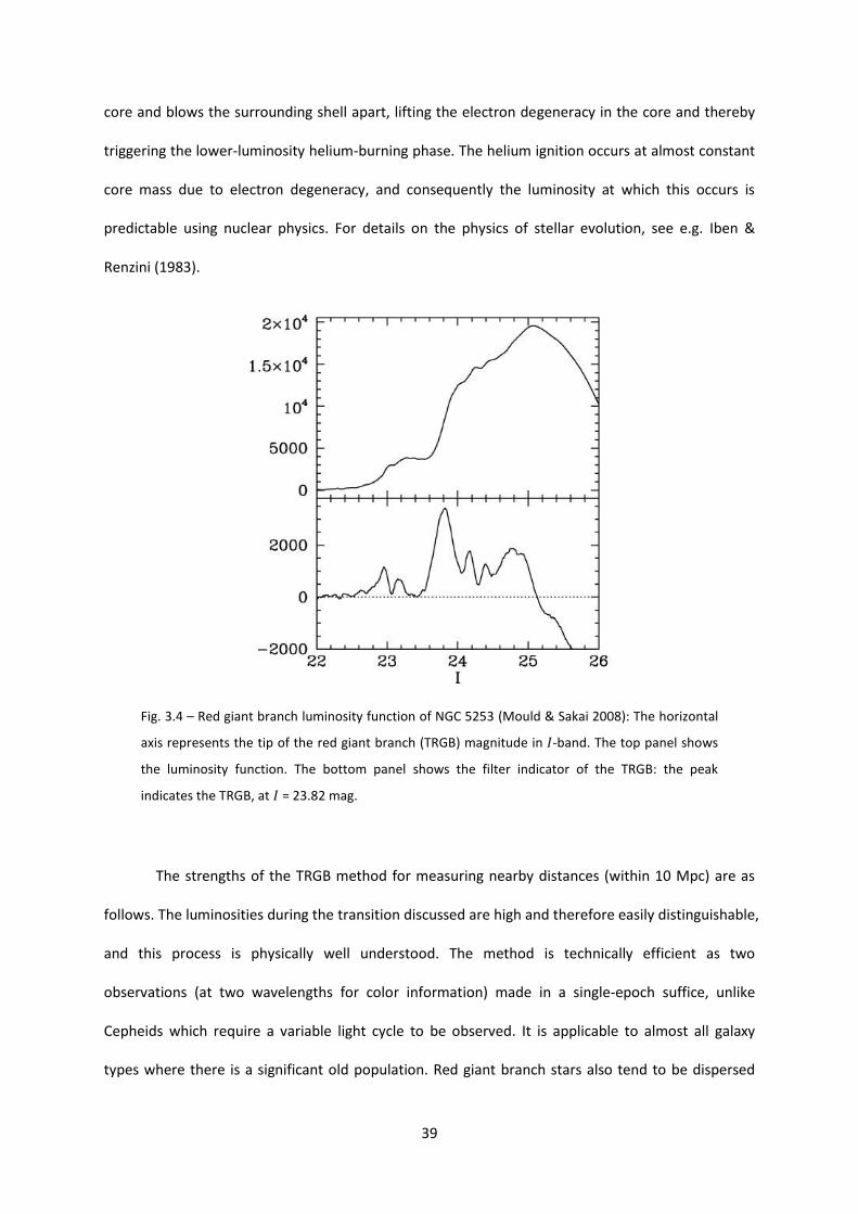
Fig. 3.4 – Red giant branch luminosity function of NGC 5253 (Mould & Sakai 2008): The horizontal

axis represents the tip of the red giant branch (TRGB) magnitude in -band. The top panel shows

the luminosity function. The bottom panel shows the filter indicator of the TRGB: the peak

indicates the TRGB, at = 23.82 mag.

The strengths of the TRGB method for measuring nearby distances (within 10 Mpc) are as

follows. The luminosities during the transition discussed are high and therefore easily distinguishable,

and this process is physically well understood. The method is technically efficient as two

observations (at two wavelengths for color information) made in a single-epoch suffice, unlike

Cepheids which require a variable light cycle to be observed. It is applicable to almost all galaxy

types where there is a significant old population. Red giant branch stars also tend to be dispersed

40

within host galaxies, reducing the systematic impact due to reddening. However, the observable

depends strongly on the metallicity of the host galaxy and weakly on the age of the stellar

population. A modern calibration of the TRGB luminosity is provided by Rizzi et al. (2007).

TRGB distance measurements can be used as an alternative to Cepheid distances in the

calibration of secondary distance indicators. Mould & Sakai (2008) use the Tully-Fisher relation

(Section 3.5) for 14 galaxies with TRGB measurements to find (statistical only) km s-1

Mpc-1, which is consistent within uncertainty allowance to the result km s-1 Mpc-1

from the Tully-Fisher relation for 21 galaxies with Cepheid measurements (Sakai et al. 2000). For the

surface brightness fluctuations method (Section 3.6), Mould & Sakai (2009a) obtain

(random) (systematic) km s-1 Mpc-1 with TRGB calibration, consistent to the result

km s-1 Mpc-1 when calibration is done using Cepheid distances. Finally, Mould & Sakai (2009b)

combine the TRGB-calibrated distances from Tully-Fisher, surface brightness fluctuations,

fundamental plane and type Ia supernovae to obtain a weighted mean for the Hubble constant

(random) (systematic) km s-1 Mpc-1, which is also consistent with the result

(random) (systematic) km s-1 Mpc-1 from a similar combination of distance

indicators but with Cepheid-calibration by Freedman et al. (2001). These results demonstrate the

consistency between TRGB and Cepheid methods.

3.5 Tully-Fisher Method

The Tully-Fisher (TF) relation is an empirical correlation between the luminosity and the

maximum rotational velocity of late-type spiral galaxies (Sakai et al. 2000). It can be generally

understood as the virial relation for rotationally supported disk galaxies with constant mass-to-light

ratio (Freedman & Madore 2010). However, its physical basis has not been firmly established: while

cold dark matter simulations suggest that the TF relation is a direct result of the cosmological

equivalence between mass and circular velocity, the dispersion due to variations in formation

41

histories is larger than what is actually observed, therefore the feedback processes regulating the

gas dynamics and stellar formation have casual effects on the TF relation (Tully & Pierce 2000).

The maximum rotational velocity is usually measured from the optical rotation curve or

radio observations of the neutral hydrogen 21 cm emission spectrum, and is distance-independent.

The TF method is applicable to thousands of distant galaxies at 100 Mpc and beyond, and is

therefore useful for Hubble constant measurements. Observations can be made at various

wavelengths, but near-infrared photometry minimizes the errors due to reddening and galaxy

morphology since infrared emission is dominated by late-type giants. The TF relation is wavelength-

dependent (see Fig. 3.5 for illustration) and is also different for field and cluster galaxies, as well as

for galaxies in different clusters.

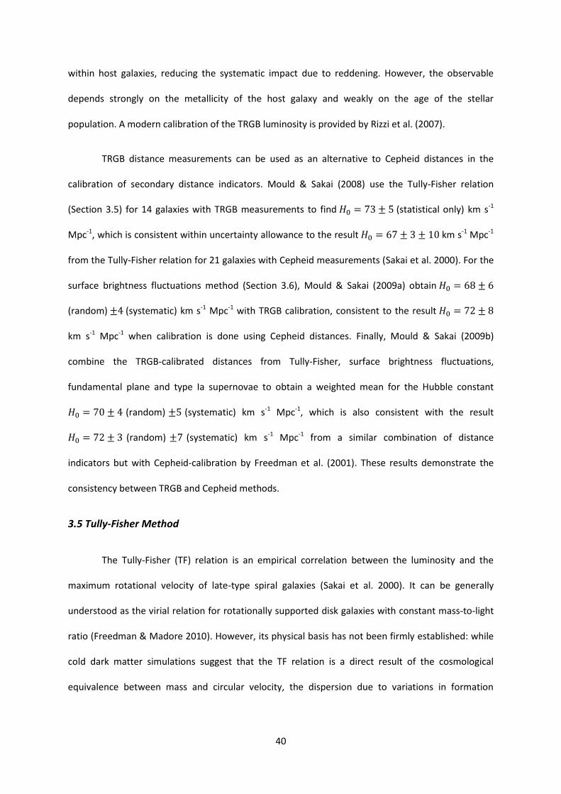
Fig. 3.5 – Tully-Fisher relations at various wavelengths for galaxies calibrated with independent

Cepheid measurements from the Hubble Space Telescope Key Project (Madore & Freedman

2010): The vertical and horizontal axes indicate the luminosity (measured by the magnitude) and

the maximum rotational velocity (typically measured by the width of a chosen spectral line) of the

spiral galaxies respectively. Panels (a) to (c) show that Tully-Fisher relations at different

wavelengths have different slopes and amounts of scatter. Panel (d) shows the Tully-Fisher

relation for a subset of 8 galaxies with luminosity observed at 3.6 μm: the small scatter suggests

that Tully-Fisher relations at this wavelength could potentially be used for high precision distance

and Hubble constant measurements, provided that the scatter would remain small when a larger

sample is considered.

42

The TF relation is typically calibrated using Cepheid distances. To determine the Hubble

constant accurately, one needs to correct for the reddening due to the inclination angle (typically

measured photometrically rather than kinematically) and the line-width of the galaxy. Approaches to

correct for the intrinsic reddening in the spiral galaxies vary as the underlying causes (e.g.

dependence on the line-width and morphology of the galaxy) are not fully understood, but

fortunately a consistent approach would suffice. Uncertainties in the derived value for the Hubble

constant are mainly due to metallicity effects on the Cepheid-calibration of the TF relation (a few

percent); variations in wavelength-dependent TF slopes used, as well as adopting different methods

to correct for intrinsic reddening and peculiar velocities, also contribute to the uncertainties in the

Hubble constant but are shown to be insignificant. Major systematics arise from the different

treatments for the zero point calibration of the TF relation and the selection biases (Malmquist and

cluster population incompleteness biases), and the resulting differences in the derived value of the

Hubble constant can be as much as km s-1 Mpc-1. Detailed analyses on this discrepancy

can be found in Sakai et al. (2000) and Tully & Pierce (2000).

Finally, Freedman & Madore (2010) observe a small intrinsic scatter in the Cepheid-

calibrated mid-infrared (3.6 μm) TF relation for 8 galaxies (Fig. 3.5d). If future observations preserve

this small scatter, potentially every TF galaxy observed in the mid-infrared could provide a distance

measurement of 5% accuracy, hence offering precision data for Hubble constant measurements.

3.6 Surface Brightness Fluctuations Method

The surface brightness fluctuations (SBF) method uses the brightness fluctuations due to a

Poissonian distribution of unresolved stars to estimate the distance to the galaxy. Specifically, the

pixel-to-pixel variance of the fluctuation is inversely proportional to the square of the distance. The

SBF measurement can be derived for an observed patch with a reasonably smooth luminosity profile,

and can be applied to galaxies as far as 100 Mpc (Biscardi et al. 2008).

43

To obtain the absolute distance (in the form of a SBF magnitude) one needs to calibrate the

SBF zero point just like other distance methods. Besides the usual Cepheid-calibration, one can also

calibrate the SBF magnitude using theoretical models. The properties of the stellar populations in

the galaxy affect the SBF magnitude, and are usually accounted for by a relation between the SBF

magnitude and the galaxy color, thereby allowing galaxies of almost any morphology to measured

using this method. Corrections are also required to remove contaminations to the observed patch,

such as dusts and foreground stars.

Biscardi et al. (2008) obtain (statistical) (systematic) km s-1 Mpc-1 using a

theoretically calibrated SBF distance scale. This agrees with km s-1 Mpc-1 from

Blakeslee et al. (2002) which calibrate SBF distances using Cepheid distances.

3.7 Masers

Cosmic maser emission occurs naturally in high density (but below the critical value for

collisional de-excitation) gas near an excitation source or a source of energy, where out-of-thermal-

equilibrium conditions readily lead to population inversion of excited atoms or molecules. Radiation

is amplified via stimulated emission as it propagates through the medium, and given the

astronomical path length this effect is significant, so that a maser emission can be luminous enough

(as high as for water masers) to be detected even from cosmological distances (Lo 2005).

Observations on maser emission from NGC 4258 give rise to a (warped) Keplerian rotating

disk model for the maser galaxy (Fig. 3.6). Maser emissions are seen, when the maser galaxy faces us

edge-on, just in front of the central continuum source and from points of the disk tangent to the line

of sight on either side of the centre, all at roughly the same radius from the centre, where the lines

of sight have the longest path with zero velocity gradient required for stimulated emission. The

proper motions of these masers, as described by their angular and absolute velocities, give the

distance to the maser galaxy. In practice, the proper motions can be inferred from high-resolution

44

observations by Very Long Baseline Interferometry (VLBI) in which masers appear as discrete peaks

in the spectrum or unresolved spots in the images. Systematics that may affect the distance

estimates include the eccentricity of the maser orbit, the source powering the masers (e.g. super-

massive black hole), radiative transfer effects (e.g. viscosity and accretion rate of disk resulting in

turbulent maser velocities), self-gravity of the disk, etc.

Fig. 3.6 – Prototype H2O maser galaxy NGC 4258 (Lo 2005): The top panel shows the spatial

distribution of the maser emission. The middle panel shows the rotation curve of the maser

emission. The bottom panel shows a three-dimensional model of a warped thin disk fitted to the

spatial distribution of the maser emission as given in the top panel.

45

Maser distance measurement to NGC 4258 agrees exactly with the Cepheid and TRGB

distances, showing its promise as an accurate alternative to SNe Ia if this accuracy holds up to

cosmological distances required for Hubble constant measurements (note that, however, NGC 4258,

at Mpc, is too close for this purpose). However, despite over 100 masers being discovered in

about 2000 galaxies so far, only about 5 of sufficient signal strengths (for current VLBI techniques)

have structures simple enough for model-fitting of the observational data to determine the distance.

The main difficulty lies in the necessity of observing the disk edge-on due to the high directionality of

maser emissions. If the method is to become viable, a significant number of maser galaxies need to

be precisely observed well into the Hubble flow. Major efforts are being undertaken through the

Megamaser Cosmology Project (Reid et al. 2009), and the Sqaure Kilometer Array is expected to

enhance the prospect of this method in future (beyond 2020).

3.8 Hubble Diagram based on Modern Distance Measurements

We conclude Section 3 by showing a Hubble diagram (Fig. 3.7) plotted with 2553 modern

accurate distance measurements using the methods discussed (Cepheids, type Ia supernovae, tip of

the red giant branch, Tully-Fisher relation, surface brightness fluctuations and masers) across 979

galaxies with known recessional velocities. The data are obtained from the online NASA/IPAC

Extragalactic Database NED-1D (Madore & Steer 2008) and are published mostly after 1990. Panels

(a) to (d) illustrate the relative ranges for various methods: the TF and SBF methods both cover up to

Mpc, while Cepheids and TRGB to Mpc and Mpc respectively; the farthest maser

distance included is at 18 Mpc; finally, note that SNe Ia are effective beyond Mpc but at such

large distances the Hubble parameter is cosmology-dependent and no longer constant. A linear

correlation consistent with a Hubble law (eq. 1.1) with km s-1 Mpc-1 is obtained (Fig. 3.7a).

The scatter is largely due to the systematics inherent in various methods, and at recessional

velocities below 5000 km s-1 peculiar motions also contribute significant errors to the observed

recessional velocities (Freedman & Madore 2010).

46

Recessional velocity / km s-1

Distance / Mpc

Recessional velocity / km s-1

Distance / Mpc

-2500

0

2500

5000

7500

10000

12500

15000

17500

20000

22500

25000

27500

30000

32500

35000

37500

0 50 100 150 200 250 300 350 400 450 500 550 600 650

Cepheid

Maser

SBF

SNIa

TRGB

TF

-1000

0

1000

2000

3000

4000

5000

6000

7000

8000

9000

10000

11000

12000

13000

0 10 20 30 40 50 60 70 80 90 100 110

Cepheid

Maser

SBF

SNIa

TRGB

TF

This segment is enlarged in the next diagram to show the ranges covered

by the Tully-Fisher (TF) and surface brightness fluctuations (SBF) methods

This segment is enlarged in the next diagram to

show the range covered by the Cepheid method

(turn to the next page)

(Fig. 3.7b)

(Fig. 3.7a)

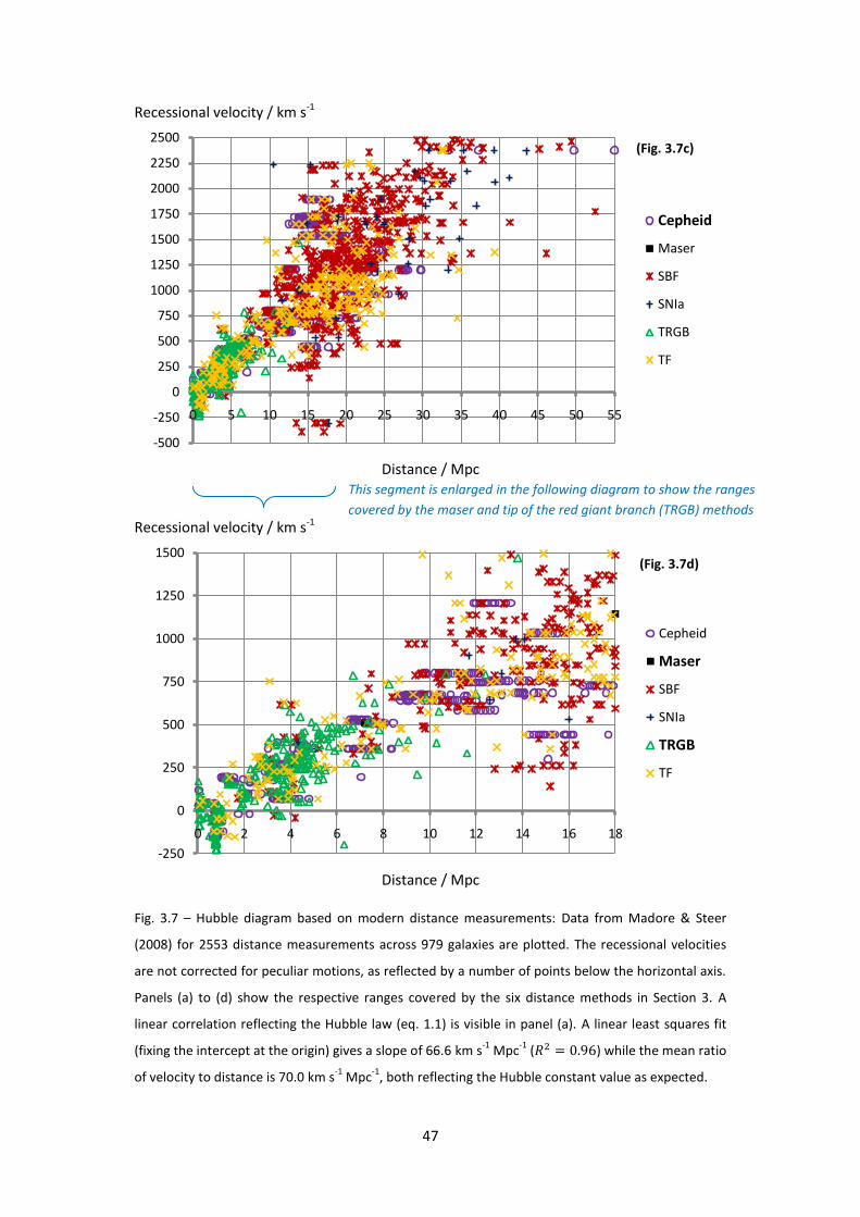
47

Recessional velocity / km s-1

Distance / Mpc

Recessional velocity / km s-1

Distance / Mpc

Fig. 3.7 – Hubble diagram based on modern distance measurements: Data from Madore & Steer

(2008) for 2553 distance measurements across 979 galaxies are plotted. The recessional velocities

are not corrected for peculiar motions, as reflected by a number of points below the horizontal axis.

Panels (a) to (d) show the respective ranges covered by the six distance methods in Section 3. A

linear correlation reflecting the Hubble law (eq. 1.1) is visible in panel (a). A linear least squares fit

(fixing the intercept at the origin) gives a slope of 66.6 km s-1

Mpc-1

( ) while the mean ratio

of velocity to distance is 70.0 km s-1

Mpc-1

, both reflecting the Hubble constant value as expected.

-500

-250

0

250

500

750

1000

1250

1500

1750

2000

2250

2500

0 5 10 15 20 25 30 35 40 45 50 55

Cepheid

Maser

SBF

SNIa

TRGB

TF

-250

0

250

500

750

1000

1250

1500

0 2 4 6 8 10 12 14 16 18

Cepheid

Maser

SBF

SNIa

TRGB

TF

This segment is enlarged in the following diagram to show the ranges

covered by the maser and tip of the red giant branch (TRGB) methods

(Fig. 3.7c)

(Fig. 3.7d)

48

4. Other Methods to Measure the Hubble Constant

4.1 Baryon Acoustic Oscillations

4.1.1 Physical Relation to the Hubble Constant

Baryon acoustic oscillations (BAO) arise from the same process that produces the cosmic

microwave background (CMB) radiation. Before recombination and decoupling, oscillations were set

up in the photon-baryon fluid by competing radiation and gravitational pressures, and density

perturbations (of this fluid) propagated outwards at a sound speed , where

(standard notations are used here: and for baryon and photon

densities, etc). Upon recombination, photons were allowed to free-stream, forming the CMB

radiation. Meanwhile, the baryon oscillations stopped as there was no longer radiation pressure on

the baryons, giving rise to fluctuations in the baryon density distribution. Over-densities have a

higher probability of forming at a characteristic length scale ( ), given by (Bassett & Hlozek 2009):

(4.1)

where (subscripts ‘eq’ and ‘rec’ indicate values as taken at equality and

recombination respectively). This characteristic scale is approximately equal to the sound horizon,

Mpc, and is an excellent standard ruler when and can be measured with high

precision. Since galaxies are more likely to form where baryon over-densities exist, the galaxy

distribution will also contain information on this characteristic scale. In this way, BAO provide a

statistical standard ruler in the form of the characteristic length scale ( ) embedded in a galaxy

distribution (observed at a particular redshift).

While other kinds of statistical standard ruler exist (e.g. Hubble scale at matter-radiation

equality and Silk damping scale), BAO can be studied primarily using linear physics. Furthermore,

since the sound horizon is well understood and determined, BAO measurements can be used in an

49

absolute Alcock-Paczynski test (Alcock & Paczynski 1979) so as to derive the Hubble rate and the

angular diameter distance (at a particular redshift where the galaxy distribution is sampled)

separately. The line-of-sight and tangential modes ( and ) of the characteristic scale are related

to the Hubble rate and angular diameter distance respectively (Fig. 4.1), as:

(4.2a)

(4.2b)

Fig. 4.1 – Schematic diagram for the Alcock-Paczynski test (Bassett & Hlozek 2009): The radial and

transverse sizes of an object are shown, where is the redshift difference between the front and

back of the object and is the angular size of the object. Where the object is spherical but with

its actual diameter unknown, the Alcock-Paczynski test enables one to determine the product

from measurements. For baryon acoustic oscillations, one can actually

theoretically compute the diameter (characteristic scale), thus the Hubble parameter and

the angular diameter distance can be determined separately using eq. (4.2a-b).

One can extract the characteristic scale ( ) from the two-point correlation function ( ) of the galaxy

distribution, which is a measure of the density difference on a given scale relative to a uniform

distribution of the same mean density. The correlation function is described approximately by a

power law ( is a spatial scale; and are constants) and reveals the characteristic

scale as a peak or dip, depending on whether there is an excess or deficiency of galaxy clustering at a

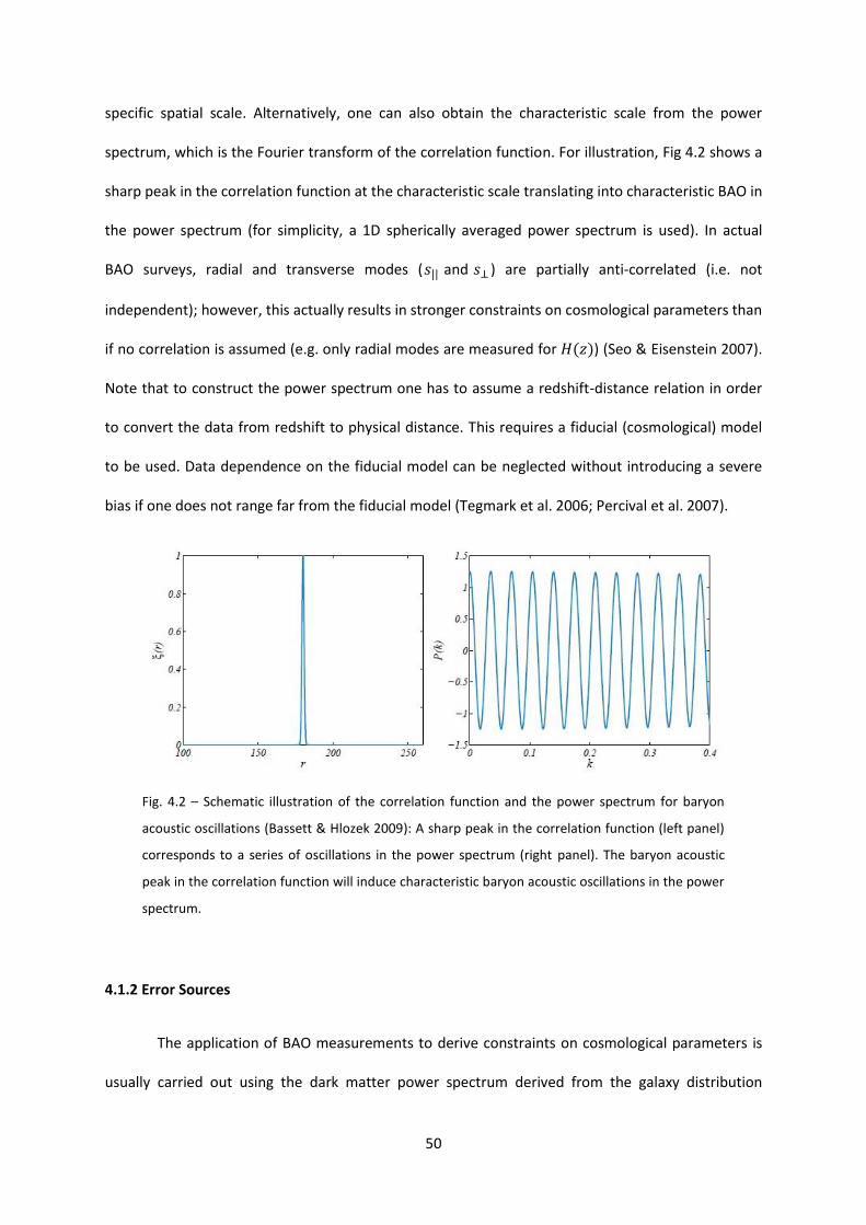
50

specific spatial scale. Alternatively, one can also obtain the characteristic scale from the power

spectrum, which is the Fourier transform of the correlation function. For illustration, Fig 4.2 shows a

sharp peak in the correlation function at the characteristic scale translating into characteristic BAO in

the power spectrum (for simplicity, a 1D spherically averaged power spectrum is used). In actual

BAO surveys, radial and transverse modes ( and ) are partially anti-correlated (i.e. not

independent); however, this actually results in stronger constraints on cosmological parameters than

if no correlation is assumed (e.g. only radial modes are measured for ) (Seo & Eisenstein 2007).

Note that to construct the power spectrum one has to assume a redshift-distance relation in order

to convert the data from redshift to physical distance. This requires a fiducial (cosmological) model

to be used. Data dependence on the fiducial model can be neglected without introducing a severe

bias if one does not range far from the fiducial model (Tegmark et al. 2006; Percival et al. 2007).

Fig. 4.2 – Schematic illustration of the correlation function and the power spectrum for baryon

acoustic oscillations (Bassett & Hlozek 2009): A sharp peak in the correlation function (left panel)

corresponds to a series of oscillations in the power spectrum (right panel). The baryon acoustic

peak in the correlation function will induce characteristic baryon acoustic oscillations in the power

spectrum.

4.1.2 Error Sources

The application of BAO measurements to derive constraints on cosmological parameters is

usually carried out using the dark matter power spectrum derived from the galaxy distribution

51

observed. As discussed in Section 4.1.1, the dark matter and galaxy distributions are largely similar in

their profiles and characteristic length scales due to gravitational coupling between dark matter and

baryons. Besides, we have well established our theoretical understanding on the relation between

the primordial dark matter and CMB spectra. In the following, we review the main error sources that

arise as one extracts the BAO characteristic scale from the dark matter distribution; the main error

sources arise from cosmic variance, shot noise, redshift and non-linearity effects.

Cosmic variance imposes fundamental limitations on the precision of our large-scale

observations due to the finite volume of the universe. On the other hand, shot noise refers to the

errors arising from the limited target density (number per unit volume of the universe) in our

observations. Targets refer to the galaxies or other discrete objects that serve as tracers to

reconstruct the dark matter distribution in the observed patch, and the accuracy of this

reconstruction increases with a higher number of tracers per unit volume of the universe observed.

The effects on the power spectrum by these two error sources cannot be minimized simultaneously.

Reducing uncertainties due to cosmic variance requires maximizing the observed volume of the

universe, but since the observation time is fixed the integration time for each observed volume will

be decreased. This is exactly the opposite of what is needed to increase the target number densities

so as to reduce shot noise. These fundamentally limit the accuracy of BAO measurements.

Another error source arises in the redshift at which our observations are made. Typically

redshifts obtained by spectroscopic means have a higher accuracy (<0.1%) than photometric means

(3-5%). However, even a smaller redshift error of 1% will lead to a significant uncertainty in BAO

measurements. Redshift errors affect only the radial position of the galaxy observed, but as the

Hubble rate is derived from the radial BAO scale its measurement will be strongly affected. In

photometric observations of BAO, redshift errors correspond to a loss in information about higher

order oscillations and therefore a smearing out of the peak in the correlation function. To improve

the photometric redshift accuracy, a greater volume of the universe needs to be surveyed.

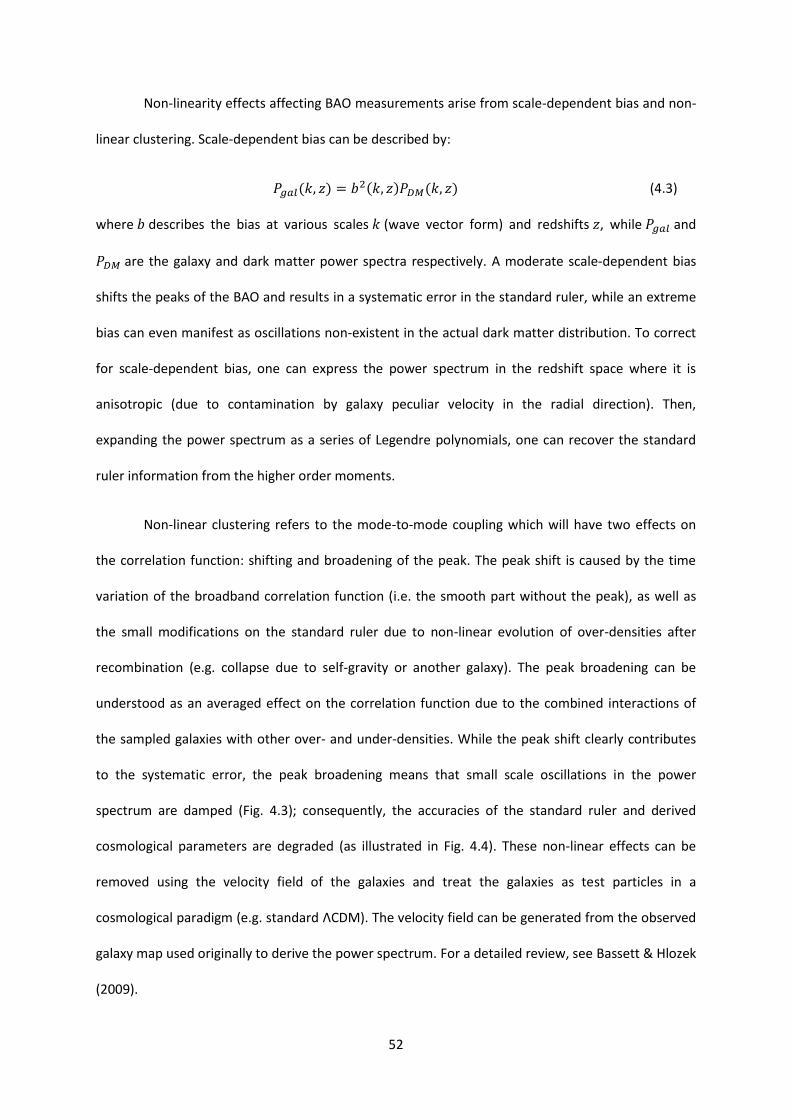
52

Non-linearity effects affecting BAO measurements arise from scale-dependent bias and non-

linear clustering. Scale-dependent bias can be described by:

(4.3)

where describes the bias at various scales (wave vector form) and redshifts , while and

are the galaxy and dark matter power spectra respectively. A moderate scale-dependent bias

shifts the peaks of the BAO and results in a systematic error in the standard ruler, while an extreme

bias can even manifest as oscillations non-existent in the actual dark matter distribution. To correct

for scale-dependent bias, one can express the power spectrum in the redshift space where it is

anisotropic (due to contamination by galaxy peculiar velocity in the radial direction). Then,

expanding the power spectrum as a series of Legendre polynomials, one can recover the standard

ruler information from the higher order moments.

Non-linear clustering refers to the mode-to-mode coupling which will have two effects on

the correlation function: shifting and broadening of the peak. The peak shift is caused by the time

variation of the broadband correlation function (i.e. the smooth part without the peak), as well as

the small modifications on the standard ruler due to non-linear evolution of over-densities after

recombination (e.g. collapse due to self-gravity or another galaxy). The peak broadening can be

understood as an averaged effect on the correlation function due to the combined interactions of

the sampled galaxies with other over- and under-densities. While the peak shift clearly contributes

to the systematic error, the peak broadening means that small scale oscillations in the power

spectrum are damped (Fig. 4.3); consequently, the accuracies of the standard ruler and derived

cosmological parameters are degraded (as illustrated in Fig. 4.4). These non-linear effects can be

removed using the velocity field of the galaxies and treat the galaxies as test particles in a

cosmological paradigm (e.g. standard ΛCDM). The velocity field can be generated from the observed

galaxy map used originally to derive the power spectrum. For a detailed review, see Bassett & Hlozek

(2009).

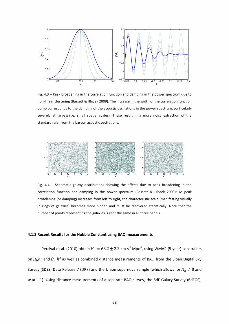
53

Fig. 4.3 – Peak broadening in the correlation function and damping in the power spectrum due to

non-linear clustering (Bassett & Hlozek 2009): The increase in the width of the correlation function

bump corresponds to the damping of the acoustic oscillations in the power spectrum, particularly

severely at large (i.e. small spatial scales). These result in a more noisy extraction of the

standard ruler from the baryon acoustic oscillations.

Fig. 4.4 – Schematic galaxy distributions showing the effects due to peak broadening in the

correlation function and damping in the power spectrum (Bassett & Hlozek 2009): As peak

broadening (or damping) increases from left to right, the characteristic scale (manifesting visually

in rings of galaxies) becomes more hidden and must be recovered statistically. Note that the

number of points representing the galaxies is kept the same in all three panels.

4.1.3 Recent Results for the Hubble Constant using BAO measurements

Percival et al. (2010) obtain km s-1 Mpc-1, using WMAP (5-year) constraints

on and

as well as combined distance measurements of BAO from the Sloan Digital Sky

Survey (SDSS) Data Release 7 (DR7) and the Union supernova sample (which allows for and

). Using distance measurements of a separate BAO survey, the 6dF Galaxy Survey (6dFGS),

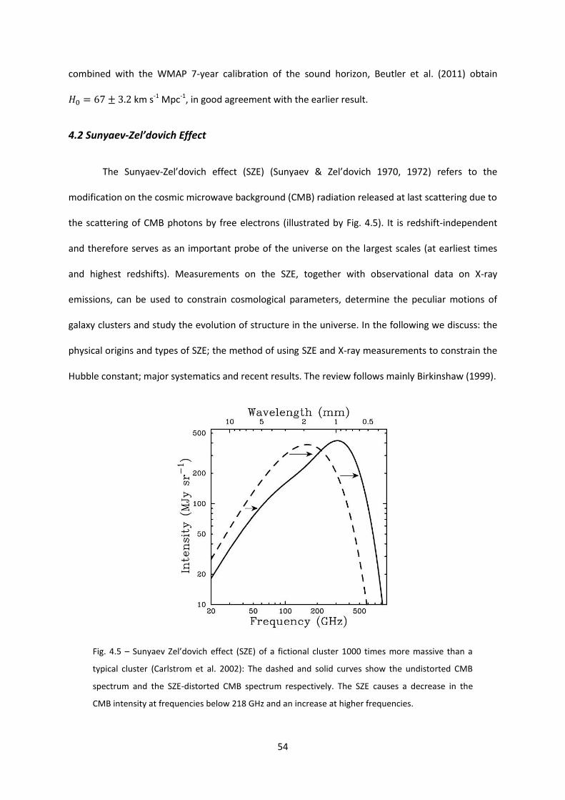
54

combined with the WMAP 7-year calibration of the sound horizon, Beutler et al. (2011) obtain

km s-1 Mpc-1, in good agreement with the earlier result.

4.2 Sunyaev-Zel’dovich Effect

The Sunyaev-Zel’dovich effect (SZE) (Sunyaev & Zel’dovich 1970, 1972) refers to the

modification on the cosmic microwave background (CMB) radiation released at last scattering due to

the scattering of CMB photons by free electrons (illustrated by Fig. 4.5). It is redshift-independent

and therefore serves as an important probe of the universe on the largest scales (at earliest times

and highest redshifts). Measurements on the SZE, together with observational data on X-ray

emissions, can be used to constrain cosmological parameters, determine the peculiar motions of

galaxy clusters and study the evolution of structure in the universe. In the following we discuss: the

physical origins and types of SZE; the method of using SZE and X-ray measurements to constrain the

Hubble constant; major systematics and recent results. The review follows mainly Birkinshaw (1999).

Fig. 4.5 – Sunyaev Zel’dovich effect (SZE) of a fictional cluster 1000 times more massive than a

typical cluster (Carlstrom et al. 2002): The dashed and solid curves show the undistorted CMB

spectrum and the SZE-distorted CMB spectrum respectively. The SZE causes a decrease in the

CMB intensity at frequencies below 218 GHz and an increase at higher frequencies.

55

4.2.1 Inverse-Compton Scattering

The scattering of photons by electrons is referred to as the inverse-Compton process. The

change in the energy and direction of a photon following an inverse-Compton scattering (by a static

electron) is given by the Compton scattering formula:

(4.4)

where and are the photon frequencies before and after the scattering, and is the deflection

angle of the photon ( is the Planck constant here). For our purpose we consider the SZE caused by

the scattering of low-energy photons by non-relativistic or mildly relativistic electrons (because, as

we will discuss in the following subsections, we rely mainly on the thermal SZE to measure the

Hubble constant). In this limit, using the logarithmic frequency shift to describe the

observed effect of the scattering ( is the observed final frequency of the photon, not equal to

due to the change in photon direction), the probability of a single scattering by an electron with

speed causing a photon frequency shift is given by:

(4.5a)

where and is the initial angle describing the photon direction (similarly, prime for final)

and is the Lorentz factor of the electron. For completeness, the other terms are given by:

(4.5b)

56

By averaging (from eq. 4.5) over the electron speed ( ) distribution, we can calculate

the distribution of photon frequency shifts for a population of electrons under inverse-Compton

scattering. For photons that have been scattered once, the probability distribution of frequency shift

is given by

(4.6)

where is the minimum value needed to cause a frequency shift and

is the electron speed distribution (common models include the relativistic Maxwellian and

power-law distributions). Further, we can obtain the distribution after scatterings from

repeated convolution integrals; for example, for photons that are scattered twice, the distribution is

(4.7)

The full frequency shift distribution includes contributions from all numbers of scatterings, i.e.

(4.8)

However, this is rarely required in most situations. In the following we will assume that the electron

scattering medium is optically thin and multiple scatterings on a photon can be neglected.

Consider an incident pure blackbody CMB spectrum, ;

the resulting CMB spectrum due to single scatterings of photons by electrons is given by

(4.9)

The above integrals can be computed to find the change in the CMB spectrum, i.e. the SZE. In the

case where we have low-energy photons, non-relativistic or mildly relativistic electrons and optically

thin scattering medium ( ), the following result can be derived:

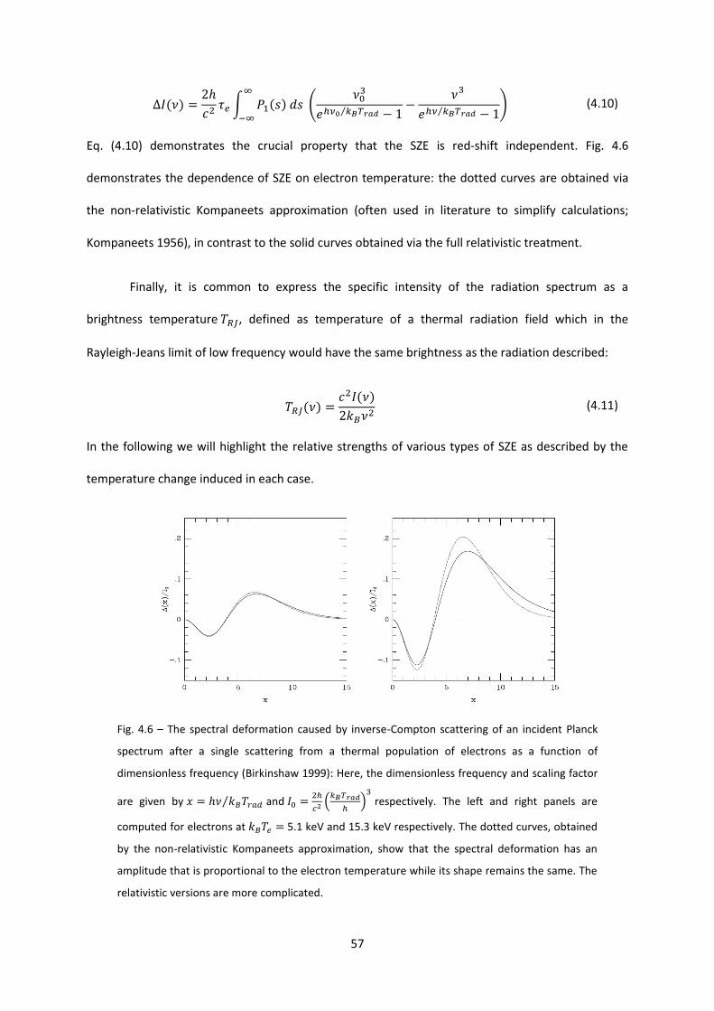
57

(4.10)

Eq. (4.10) demonstrates the crucial property that the SZE is red-shift independent. Fig. 4.6

demonstrates the dependence of SZE on electron temperature: the dotted curves are obtained via

the non-relativistic Kompaneets approximation (often used in literature to simplify calculations;

Kompaneets 1956), in contrast to the solid curves obtained via the full relativistic treatment.

Finally, it is common to express the specific intensity of the radiation spectrum as a

brightness temperature , defined as temperature of a thermal radiation field which in the

Rayleigh-Jeans limit of low frequency would have the same brightness as the radiation described:

(4.11)

In the following we will highlight the relative strengths of various types of SZE as described by the

temperature change induced in each case.

Fig. 4.6 – The spectral deformation caused by inverse-Compton scattering of an incident Planck

spectrum after a single scattering from a thermal population of electrons as a function of

dimensionless frequency (Birkinshaw 1999): Here, the dimensionless frequency and scaling factor

are given by and

respectively. The left and right panels are

computed for electrons at 5.1 keV and 15.3 keV respectively. The dotted curves, obtained

by the non-relativistic Kompaneets approximation, show that the spectral deformation has an

amplitude that is proportional to the electron temperature while its shape remains the same. The

relativistic versions are more complicated.

58

4.2.2 Thermal SZE

Inverse-Compton scattering occurs where there is an electron population with significant

energy content, mainly in the atmospheres of clusters and superclusters of galaxies as well as in the

ionized regions of the universe and ionized gas near us. Thermal SZE refers to that which arises from

electron populations that are not highly relativistic (and can be studied using the Kompaneets

approximation). Thermal SZE arising from the atmospheres of galaxy clusters is the most common

and dominant source of SZE. The existence of the electron population can be detected through its X-

ray emission or effects on radio source morphologies (e.g. disturbed lobe shapes, head-tail sources).

To describe the electron population such that its SZE and X-ray spectrum can be studied, the

following parameters are mainly used: the electron concentration ; scattering optical depth ;

Comptonization parameter ; and X-ray spectral surface brightness along the line of sight . They

are defined as follows:

(4.12a)

(4.12b)

(4.12c)

In the above, is the redshift of the cluster; is the spectral emissivity of the electron gas (assumed

to be isotropic) at observed X-ray energy ; is the path length and integrations are over the spatial

extension of the election gas; and is the Thomson cross-section which characterizes the strength

of the non-relativistic scattering process. With observational data from X-ray emission providing

information on , one can predict the SZE of the cluster (i.e. find and , and hence and )

if a parameterized model is adopted to fit the X-ray data. A common choice is the isothermal

model in which the electron temperature is constant and the electron number density follows the

spherical distribution:

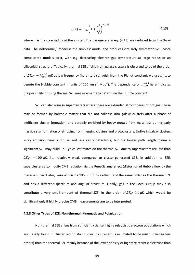
59

(4.13)

where is the core radius of the cluster. The parameters in eq. (4.13) are deduced from the X-ray

data. The isothermal model is the simplest model and produces circularly symmetric SZE. More

complicated models exist, with e.g. decreasing electron gas temperature at large radius or an

ellipsoidal structure. Typically, thermal SZE arising from galaxy clusters is observed to be of the order

of mK at low frequency (here, to distinguish from the Planck constant, we use to

denote the Hubble constant in units of 100 km s-1 Mpc-1). The dependence on here indicates

the possibility of using thermal SZE measurements to determine the Hubble constant.

SZE can also arise in superclusters where there are extended atmospheres of hot gas. These

may be formed by baryonic matter that did not collapse into galaxy clusters after a phase of

inefficient cluster formation, and partially enriched by heavy metals from mass loss during early

massive star formation or stripping from merging clusters and protoclusters. Unlike in galaxy clusters,

X-ray emission here is diffuse and less easily detectable, but the longer path length means a

significant SZE may build up. Typical estimates on the thermal SZE due to superclusters are less than

μK, i.e. relatively weak compared to cluster-generated SZE. In addition to SZE,

superclusters also modify CMB radiation via the Rees-Sciama effect (distortion of Hubble flow by the

massive supercluster; Rees & Sciama 1968), but this effect is of the same order as the thermal SZE

and has a different spectrum and angular structure. Finally, gas in the Local Group may also

contribute a very small amount of thermal SZE, in the order of μK which would be

significant only if highly precise CMB measurements are to be interpreted.

4.2.3 Other Types of SZE: Non-thermal, Kinematic and Polarization

Non-thermal SZE arises from sufficiently dense, highly relativistic electron populations which

are usually found in cluster radio halo sources. Its strength is estimated to be much lower (a few

orders) than the thermal SZE mainly because of the lower density of highly relativistic electrons than

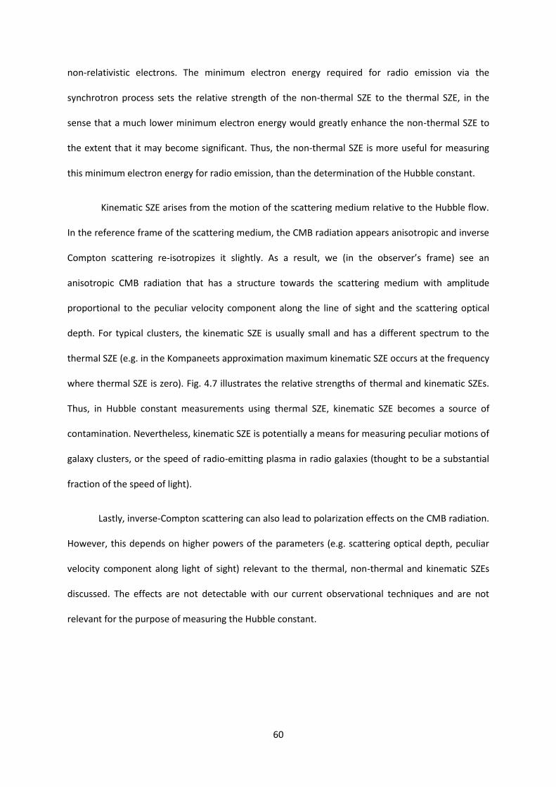
60

non-relativistic electrons. The minimum electron energy required for radio emission via the

synchrotron process sets the relative strength of the non-thermal SZE to the thermal SZE, in the

sense that a much lower minimum electron energy would greatly enhance the non-thermal SZE to

the extent that it may become significant. Thus, the non-thermal SZE is more useful for measuring

this minimum electron energy for radio emission, than the determination of the Hubble constant.

Kinematic SZE arises from the motion of the scattering medium relative to the Hubble flow.

In the reference frame of the scattering medium, the CMB radiation appears anisotropic and inverse

Compton scattering re-isotropizes it slightly. As a result, we (in the observer’s frame) see an

anisotropic CMB radiation that has a structure towards the scattering medium with amplitude

proportional to the peculiar velocity component along the line of sight and the scattering optical

depth. For typical clusters, the kinematic SZE is usually small and has a different spectrum to the

thermal SZE (e.g. in the Kompaneets approximation maximum kinematic SZE occurs at the frequency

where thermal SZE is zero). Fig. 4.7 illustrates the relative strengths of thermal and kinematic SZEs.

Thus, in Hubble constant measurements using thermal SZE, kinematic SZE becomes a source of

contamination. Nevertheless, kinematic SZE is potentially a means for measuring peculiar motions of

galaxy clusters, or the speed of radio-emitting plasma in radio galaxies (thought to be a substantial

fraction of the speed of light).

Lastly, inverse-Compton scattering can also lead to polarization effects on the CMB radiation.

However, this depends on higher powers of the parameters (e.g. scattering optical depth, peculiar

velocity component along light of sight) relevant to the thermal, non-thermal and kinematic SZEs

discussed. The effects are not detectable with our current observational techniques and are not

relevant for the purpose of measuring the Hubble constant.

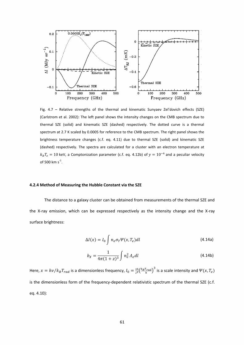
61

Fig. 4.7 – Relative strengths of the thermal and kinematic Sunyaev Zel’dovich effects (SZE)

(Carlstrom et al. 2002): The left panel shows the intensity changes on the CMB spectrum due to

thermal SZE (solid) and kinematic SZE (dashed) respectively. The dotted curve is a thermal

spectrum at 2.7 K scaled by 0.0005 for reference to the CMB spectrum. The right panel shows the

brightness temperature changes (c.f. eq. 4.11) due to thermal SZE (solid) and kinematic SZE

(dashed) respectively. The spectra are calculated for a cluster with an electron temperature at

keV, a Comptonization parameter (c.f. eq. 4.12b) of and a peculiar velocity

of 500 km s-1

.

4.2.4 Method of Measuring the Hubble Constant via the SZE

The distance to a galaxy cluster can be obtained from measurements of the thermal SZE and

the X-ray emission, which can be expressed respectively as the intensity change and the X-ray

surface brightness:

(4.14a)

(4.14b)

Here, is a dimensionless frequency,

is a scale intensity and

is the dimensionless form of the frequency-dependent relativistic spectrum of the thermal SZE (c.f.

eq. 4.10):

62

(4.15)

where . The expression for is the same as that in eq. (4.12c).

As the thermal SZE and X-ray emission depend on and respectively, the ratio of

gives a density-weighted measure of the path-length through the electron gas. Thus, if the

gas structure is known, then we can determine its angular size and therefore the angular diameter

distance to the galaxy cluster. One way to model the electron gas structure is to express various

parameters in combinations of reference values (at the centre or any fiducial point) and

dimensionless form factors ( ), an example as follows:

(4.16)

where is the angle between the reference line of sight and cluster center, is the azimuthal angle

about the line of sight, and gives an angular measure of distance along the line of sight (

is the angular diameter distance of the cluster). The SZE and X-ray emission (eq. 4.14a-b) can then be

re-expressed as:

(4.17a)

(4.17b)

Adopting a parameterized model (e.g. the isothermal model (eq. 4.13) and using observational

data for SZE and X-ray, the values of and can be deduced. Using eq. (4.17a-b), we can

calculate the angular diameter distance of the cluster:

(4.18)

63

The Hubble constant can then be determined using the angular diameter distance and measured

redshift of the cluster (with assumed values of the deceleration parameter and the

cosmological constant, which is taken to be zero below):

(4.19)

4.2.5 Major Systematics

Unlike other distance methods to determine the Hubble constant, this method can be used

to measure cosmological distances directly without using a distance ladder, therefore avoiding

systematics due to other distance indicators. This method is based on simple physics of a fully

ionized gas in hydrostatic equilibrium within the gravitational potential well of a galaxy cluster, and

hence the accuracy of the distance estimated depends only on how well we can understand and

model the intracluster gas. However, because the form factors (eq. 4.16) cannot be determined from

the SZE and X-ray data which have been used to determine and in the first place, substantial

systematics can arise due to model imperfections – e.g. form factors in (eq. 4.16) are inadequate if

there exists much small-scale structure in the cluster gas.

The most serious source of systematics is due to a selection bias in favor of clusters

elongated along the line of sight (instead of being spherically symmetric as assumed in convenient

models). Their X-ray and SZ effects are easier to detect due to the higher central surface brightness

in the elongated gas distributions, and observational images cannot distinguish them from

spherically symmetric ones if the gas distributions have a symmetry axis along the line of sight. The

above method, i.e. adopting a model that assumes spherical symmetry (Section 4.2.4), will result in a

biased estimate for the angular diameter distance:

(4.20)

where is the factor describing how much the distribution is elongated along the line of sight in

comparison with other directions. This can cause a large downward bias in the resulting estimate for

64

the Hubble constant (probably up to 30%). To minimize this error, the sample should include clusters

over a wide range of luminosities instead of just the brightest ones with the most detectable X-ray

and SZEs. Besides the elongation of gas distribution along the line of sight, intrinsic irregularities in

the cluster atmospheres may also contribute to a systematic error of as much as 20% in the Hubble

constant derived.

Another major source of systematics arises from the uncertainties in the model parameters

which depend on the accuracies of the observational data that the parameters are fitted upon. The

gas models adopted may also not capture every detail of the gas structure, hence contributing to the

systematics as well. The effects due to model imperfections are important because the X-ray and SZE

spectra are dominated by different parts of the gas. The X-ray surface brightness is dominated by the

densest parts of the clusters as X-ray emissivity is proportional to

, but the SZE is dominated

by the less dense and hotter parts where the path lengths are longest. To minimize this error,

observations need to capture a sufficiently large angular scale so as to include (ideally) all parts of

the gas that contribute strongly to either X-ray or SZE spectra. In practice, this requires tracing the X-

ray emission out to a radius where the surface brightness is a few orders lower than the core value.

While isothermal models are usually used, realistically they cannot describe completely the

thermal structure of the cluster gas. Furthermore, as mentioned measurements should be made at

outermost parts of the gas where the X-ray surface brightness is very low and current instruments

are not sensitive enough to determine temperature changes at such regions. This is expected to

contribute systematics at the 10% level; in fact, hydrodynamical models of the evolution of cluster

atmospheres (Roettiger et al. 1997; Yoshikawa et al. 1998) suggest that extreme non-isothermality

can cause up to 30% systematic and 10% random errors in the Hubble constant. However, recent

results by Bonamente et al. (2006) suggest that (using a sufficiently large sample) the effects of non-

isothermality under hydrostatic equilibrium conditions are not as significant as previously expected.

65

A cooling flow towards the core of the gas can introduce errors due to the large change of

gas properties in the core which the model adopted (eq. 4.16) does not account for. High X-ray

emissivity of the core means the gas cools more rapidly than gases elsewhere. This results in a drop

in core pressure and hence the cooling flow of surrounding gases towards the core. The core X-ray

emissivity increases further while temperature decreases. Since the affected core region is spatially

small, this error can be minimized by excluding the core data when using the parameterized model

to determine the Hubble constant.

Small-scale clumping in the gas structure, unresolved by observations, will lead to an

underestimated angular diameter distance and therefore overestimate the Hubble constant. This is

because (for an isothermal gas) density clumping enhances the X-ray emissivity of a small gas

element by a factor

, but the SZE is unaffected since is unchanged.

Significant systematics will arise if is or higher. This error cannot be reduced by using a

larger sample as in the case of the selection bias due to elongated gas distributions, because all

cluster atmospheres will be clumpy to some degree. One therefore should estimate or measure the

average clumping in a cluster so as to correct for it. However, this is theoretically challenging as one

will have to understand the processes that cause as well as negate clumping (e.g. gas injection from

galaxies and energy input from galaxy motions for the former, thermal conduction and gas dynamics

for the latter). Fortunately, current observations suggest that clumping is usually weak: if was

often large then variations in the degree of clumping among clusters would also be significant; the

resultant Hubble diagram would have a strong scatter, but this is not observed.

Additional errors can arise from various sources of contamination on the SZE as well as X-ray

emission. Potential SZE contaminations include: a background primordial anisotropy in the CMB

radiation spectrum; the non-thermal SZE by a cluster radio halo source; the kinematic SZE; and

diffuse radio emission from cool gas towards the edge of the cluster. Meanwhile, the X-ray emission

66

can be contaminated by the inverse-Compton emission of relativistic electrons in the cluster radio

halo source. These effects can contribute to up to 10% errors (systematic plus random).

4.2.6 Recent Results for the Hubble Constant Measured via the SZE

A recent determination of the Hubble constant using SZE and X-ray emission measurements

is provided by Bonamente et al. (2006). Data on 38 galaxy clusters in the redshift range

are analysed via a Markov chain Monte Carlo technique that provides simultaneous estimation

of all model parameters, firstly by adopting a hydrostatic equilibrium model that accounts for radial

variations in density and temperature due to cooling at the gas core, and then by the simpler

isothermal model. Assuming a universe with and , they obtain the values of

km s-1 Mpc-1 for the hydrostatic equilibrium model and

km s-1

Mpc-1 for the isothermal model (statistical followed by systematic uncertainties at 68% confidence

level for both results). The good agreement between the two models suggests that when using the

SZE method to measure the Hubble constant, the simpler isothermal model would suffice under

current observational sensitivities.

4.3 Gravitational Lens Time Delays

4.3.1 Fundamental Principles

Measured time delays between multiple images (of the same source) due to a gravitational

lens system provide an independent means of determining the Hubble constant. Such gravitational

lens systems include multiple quasars (double, triple and quadruple images of a single quasar), arcs

(images of high redshift galaxies formed by deep cluster potential wells) and radio rings (images of

extended radio sources formed by intervening galaxies) (Blandford & Narayan 1992). As discussed

below, the relative time delay between the images is inversely proportional to the Hubble constant

via a combination of angular diameter distances, and depends strongly on the lens mass distribution

but weakly on other cosmological parameters. Thus, we can infer the value for the Hubble constant

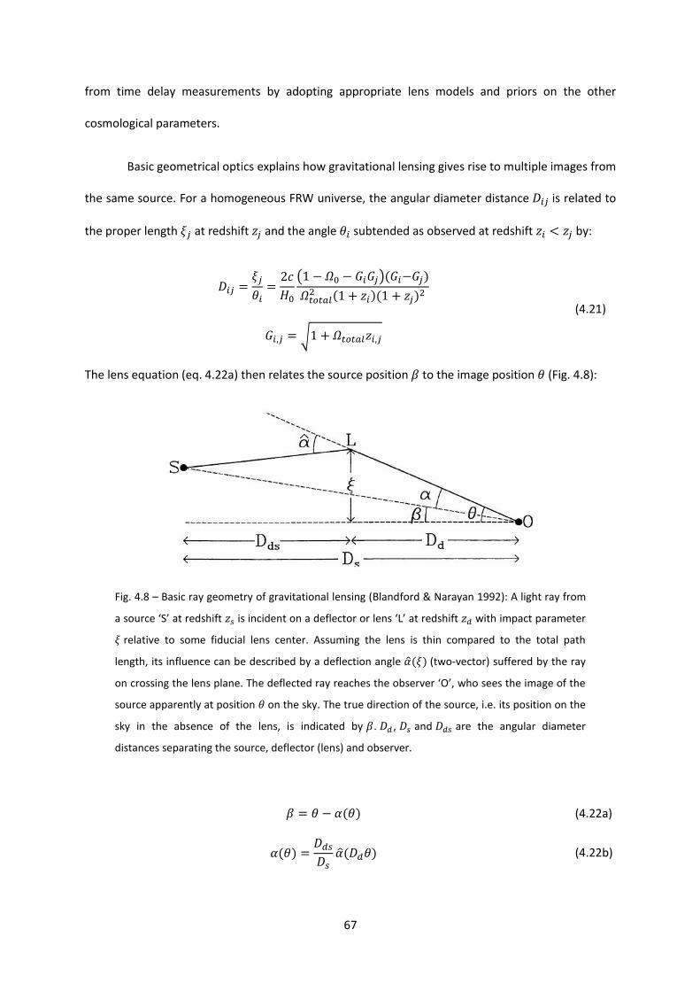
67

from time delay measurements by adopting appropriate lens models and priors on the other

cosmological parameters.

Basic geometrical optics explains how gravitational lensing gives rise to multiple images from

the same source. For a homogeneous FRW universe, the angular diameter distance is related to

the proper length at redshift and the angle subtended as observed at redshift by:

(4.21)

The lens equation (eq. 4.22a) then relates the source position to the image position (Fig. 4.8):

Fig. 4.8 – Basic ray geometry of gravitational lensing (Blandford & Narayan 1992): A light ray from

a source ‘S’ at redshift is incident on a deflector or lens ‘L’ at redshift with impact parameter

relative to some fiducial lens center. Assuming the lens is thin compared to the total path

length, its influence can be described by a deflection angle (two-vector) suffered by the ray

on crossing the lens plane. The deflected ray reaches the observer ‘O’, who sees the image of the

source apparently at position on the sky. The true direction of the source, i.e. its position on the

sky in the absence of the lens, is indicated by . , and are the angular diameter

distances separating the source, deflector (lens) and observer.

(4.22a)

(4.22b)

68

where is the reduced deflection angle and is the true deflection angle, and the above

angles are three-dimensional vector quantities (not scalars). The true deflection angle depends on

the lens mass distribution, and the dependence is governed by General Relativity. In the weak field

limit (applicable here since deflections are small) for a thin lens, where is a 2D

Newtonian potential determined by the surface mass density via the Poisson equation

. Multiple images arise when nontrivial allows more than one solutions for for a single

source in eq. (4.22).

We illustrate this with two examples in the opposite extremes: lensing by a point mass and

lensing by a mass distribution of a length scale much larger than that of the image region. In the case

of a point mass lens, a source on the optical axis will form an Einstein ring. An off-axis source will

produce two images on opposite sides of the lens (respective magnification on each image depends

on where the source lies with respect to the Einstein ring, thus lensing leads to image distortion for

an extended source). In the case of a lens formed by a widely extended mass distribution, if we

expand the potential to the quadratic order (i.e. considering a quadratic lens) then the

magnification consists of an isotropic part (parameterized by the convergence) and an anisotropic

part (parameterized by the shear). Normally, multiple images are produced when the lens has

regions with convergence greater than a critical value. In more realistic situations where the

universe may not even be homogeneous and the lens system is more complex, the number of

images by a source (or image multiplicity) depends on where the source lies with respect to the

caustics, which is the 2D surface where the magnification diverges formally, and generally separates

regions with image multiplicities differing by two.

The propagation time from the source to the observer can vary for different images due to

differences in geometrical path length and gravitational potential along the path, and this time-

difference can be measured if the source is variable. For a single lens in a homogeneous universe,

69

the excess time delay of an image at relative to the time without lensing ( labels the images) is

given by:

(4.23)

where the first term describes the geometric delay while the second describes the gravitational

delay (Shapiro effect). We can see that eq. (4.23) is consistent with the Fermat’s principle for photon

propagation since the extremal time (obtained by differentiating eq. (4.23) and solving for zero

derivative) occurs where the lens equation (eq. 4.22) with is satisfied. While the above

quantity cannot be measured, the relative time delay between two images, can be.

From the dependence on in (eq. 4.21), we can see that measurements on the relative time

delay (which is inversely proportional to ) allow us to determine the Hubble constant directly.

4.3.2 Constraints, Degeneracies and Other Difficulties

As we do not have a priori information on the exact form of lens potential in eq. (4.23),

we have to introduce parameterized models to fit with observational data so as to infer the time

delays and the Hubble constant. The detail or complexity to which we can model the gravitational

lensing system is restricted not only by our theoretical knowledge on the astrophysical objects

constituting the lensing system, but also the quantity and quality of our observational data. The

number of parameters should be at most equal to the number of constraints derived from the

observational data, otherwise we could always obtain a perfect fit without being able to check the

goodness of fit (using the excess constraints after the model parameters are determined) (Schechter

2005). In the case where we have resolved images (from, say, the lensing of a quasar), available

constraints are generated by measurements of the relative time delays ( ), image deflections

( ) and distortions ( ). Although delay (scalar), deflection (vector) and distortion (matrix)

each have one, two and three independent elements respectively, not all can contribute to the

available constraints for our model parameters since essentially all our measurements are relative in

70

nature – we do not know the absolute propagation time, the actual position or the exact shape and

size of the source. Furthermore, one constraint generated from the relative time delay has to be

reserved for the determination of the Hubble constant. Thus, the number of available constraints for

the model parameters is as shown in Table 4.1 below (Schechter 2005). In the case when the sources

are unresolved, we have even less available constraints from observational data because instead of

distortion (three elements) we can only measure the magnification (one element).

Observable Number of Constraints

Delay 1 × (no. of images – 2)

Deflection 2 × (no. of images – 1)

Distortion (if sources are resolved) 3 × (no. of images – 1)

Magnification (if sources are unresolved) 1 × (no. of images – 1)

Table 4.1: Number of constraints on model parameters that can be derived from observables

Furthermore, there exist degeneracies in the lens modeling that, if left unbroken, lead to

large variations in the Hubble constant prediction. The most serious is the mass-sheet degeneracy.

One can add a mass-sheet (with zero shear contributions) to the model such that the predicted

image positions remain unchanged (i.e. fitting the observations). However, the additional mass-

sheet will lead to a different relative time delay via its effects on the lens potential (through the

mean convergence), thus resulting in a different Hubble constant prediction (Suyu et al. 2010). The

mass-sheet degeneracy can be broken by information (in addition to lensing observations) on one of

following: the intrinsic magnitude or angular size of the source; the mass of the lensing system (mass

normalization); or the external convergence of the lensing system. The first is often unavailable for

sources observed through the gravitational lensing method. To understand the remaining two

options, we first note that mass-sheets can be classified as internal or external: internal mass-sheets

are galaxies, groups or clusters that are close enough to the lens galaxy such that they affect the

stellar dynamics of the latter; external mass-sheets, in contrast, are those who do not affect the

stellar dynamics of the lens galaxy. The external convergence is associated solely with the external

71

mass sheets. For a given stellar velocity dispersion, there is a degeneracy in the mass and the stellar

orbit anisotropy which is nearly orthogonal to the mass-sheet degeneracy. One can then break the

mass-sheet degeneracy by estimating the total mass of the internal mass-sheets using observational

data on the stellar velocity dispersion and lensing together. Alternatively, one can observe the

region around, as well as along the line of sight to, the lens galaxy to model the external mass

distribution, and therefore estimate the external convergence in order to break the mass-sheet

degeneracy. For details on how these work, refer to Suyu et al. (2010) and the references within.

There are other parameter degeneracies that affect the determination of the Hubble

constant. A notable example is the central concentration degeneracy which arises when there is a

lack of information about the internal structure of the lensing galaxy. When using power laws to

describe the mass distribution along the radial distance from the centre of the lens, the predicted

value of the Hubble constant is often degenerate with the radial slope in the mass profile. This

degeneracy can be broken if the radial slope can be determined from, for example, precise

observations of extended images.

Another challenge can arise in the form of multiple lensing, when there is more than one

lensing galaxy along the line of sight to the sources. Essentially the modeling of such a multiple

lensing system is difficult and the resulting Hubble constant prediction can vary significantly. This

issue is present even when one of the lenses is far more dominant than the rest, because path

lengths are highly sensitive to shifts in the centre of mass of the entire lensing system, hence the

predicted time delays can still be much affected. Difficulties can arise in the modeling of the

distribution of non-baryonic matter between lens galaxies (with possible dynamical interactions

between the lens galaxies), the respective features and details of the galaxies (e.g. the halos, the

central positions), etc. However, on a positive note, multiple lensing provides an observational

advantage as more images are actually produced (Schechter 2005), therefore offering more

empirical information to narrow down plausible theoretical descriptions.

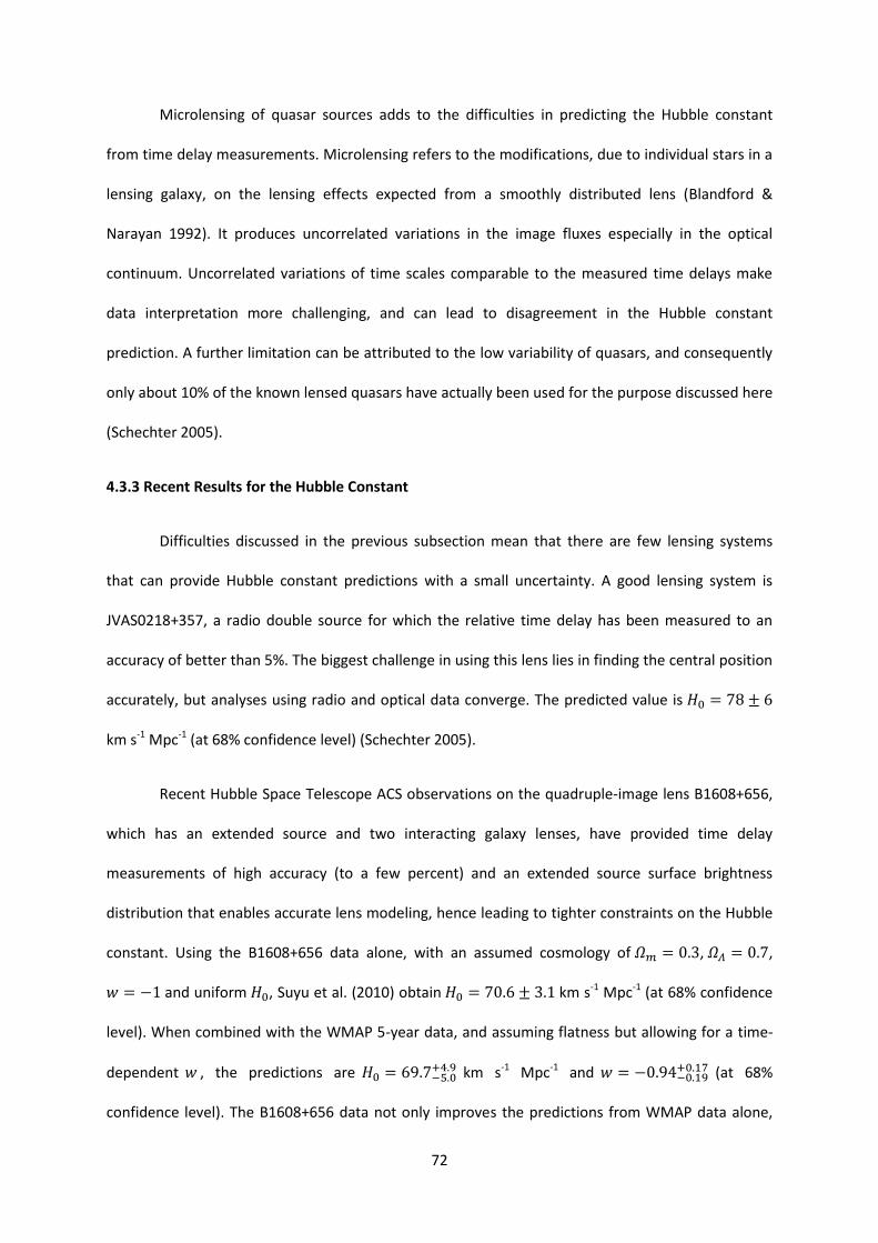
72

Microlensing of quasar sources adds to the difficulties in predicting the Hubble constant

from time delay measurements. Microlensing refers to the modifications, due to individual stars in a

lensing galaxy, on the lensing effects expected from a smoothly distributed lens (Blandford &

Narayan 1992). It produces uncorrelated variations in the image fluxes especially in the optical

continuum. Uncorrelated variations of time scales comparable to the measured time delays make

data interpretation more challenging, and can lead to disagreement in the Hubble constant

prediction. A further limitation can be attributed to the low variability of quasars, and consequently

only about 10% of the known lensed quasars have actually been used for the purpose discussed here

(Schechter 2005).

4.3.3 Recent Results for the Hubble Constant

Difficulties discussed in the previous subsection mean that there are few lensing systems

that can provide Hubble constant predictions with a small uncertainty. A good lensing system is

JVAS0218+357, a radio double source for which the relative time delay has been measured to an

accuracy of better than 5%. The biggest challenge in using this lens lies in finding the central position

accurately, but analyses using radio and optical data converge. The predicted value is

km s-1 Mpc-1 (at 68% confidence level) (Schechter 2005).

Recent Hubble Space Telescope ACS observations on the quadruple-image lens B1608+656,

which has an extended source and two interacting galaxy lenses, have provided time delay

measurements of high accuracy (to a few percent) and an extended source surface brightness

distribution that enables accurate lens modeling, hence leading to tighter constraints on the Hubble

constant. Using the B1608+656 data alone, with an assumed cosmology of , ,

and uniform , Suyu et al. (2010) obtain km s-1 Mpc-1 (at 68% confidence

level). When combined with the WMAP 5-year data, and assuming flatness but allowing for a time-

dependent , the predictions are km s-1 Mpc-1 and

(at 68%

confidence level). The B1608+656 data not only improves the predictions from WMAP data alone,

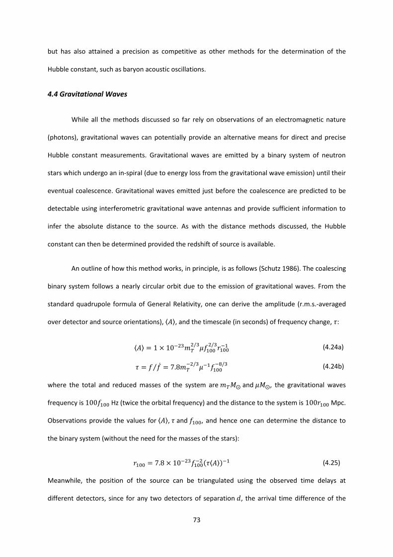
73

but has also attained a precision as competitive as other methods for the determination of the

Hubble constant, such as baryon acoustic oscillations.

4.4 Gravitational Waves

While all the methods discussed so far rely on observations of an electromagnetic nature

(photons), gravitational waves can potentially provide an alternative means for direct and precise

Hubble constant measurements. Gravitational waves are emitted by a binary system of neutron

stars which undergo an in-spiral (due to energy loss from the gravitational wave emission) until their

eventual coalescence. Gravitational waves emitted just before the coalescence are predicted to be

detectable using interferometric gravitational wave antennas and provide sufficient information to

infer the absolute distance to the source. As with the distance methods discussed, the Hubble

constant can then be determined provided the redshift of source is available.

An outline of how this method works, in principle, is as follows (Schutz 1986). The coalescing

binary system follows a nearly circular orbit due to the emission of gravitational waves. From the

standard quadrupole formula of General Relativity, one can derive the amplitude (r.m.s.-averaged

over detector and source orientations), , and the timescale (in seconds) of frequency change, :

(4.24a)

(4.24b)

where the total and reduced masses of the system are and , the gravitational waves

frequency is Hz (twice the orbital frequency) and the distance to the system is Mpc.

Observations provide the values for , and , and hence one can determine the distance to

the binary system (without the need for the masses of the stars):

(4.25)

Meanwhile, the position of the source can be triangulated using the observed time delays at

different detectors, since for any two detectors of separation , the arrival time difference of the

74

wave is , where is the angle subtended by the lines joining the source to each

detector. Taking into account further effects on the observed time delays due to the polarizations of

the individual detectors (linear) and the waves (elliptical), one can determine completely the five

unknowns of the waves (namely, two arrival directions, two amplitudes for different polarizations

and one phase difference of the polarizations) using three detectors (which provide two

independent time-delay and three amplitude measurements). In this way, one may be able to

determine the position accurately so that one can separately identify the galaxy and its redshift for

the Hubble constant to be determined. In practice, obtaining the position and redshift of the source

galaxy poses the biggest challenge for this method, and various statistical approaches are developed

(e.g. Chernoff & Finn 1993, MacLeod & Hogan 2008, Del Pozzo 2011).

In principle, this method has the potential to determine the Hubble constant to accuracies at

the few percent level. The underlying physics is relatively simple and immune to systematics

suffered by electromagnetic observational techniques, thus this method complements the other

methods discussed previously. A drawback is the low and highly uncertain event rate for the

coalescence of binary systems: based on the birth rate of pulsars, which are the only compact-object

binary systems known with a lifetime of years, there will be events per year out to 100

Mpc but the actual rate may fluctuate by a factor of 10 (Schutz 1986). In general, an increased

sample improves the accuracy of the Hubble constant prediction, thus an observational time of a

few years may be required to reduce the Hubble constant uncertainty to a few percent. Improved

observational techniques that measure the position and redshift more accurately will help to

shorten the observational time needed.

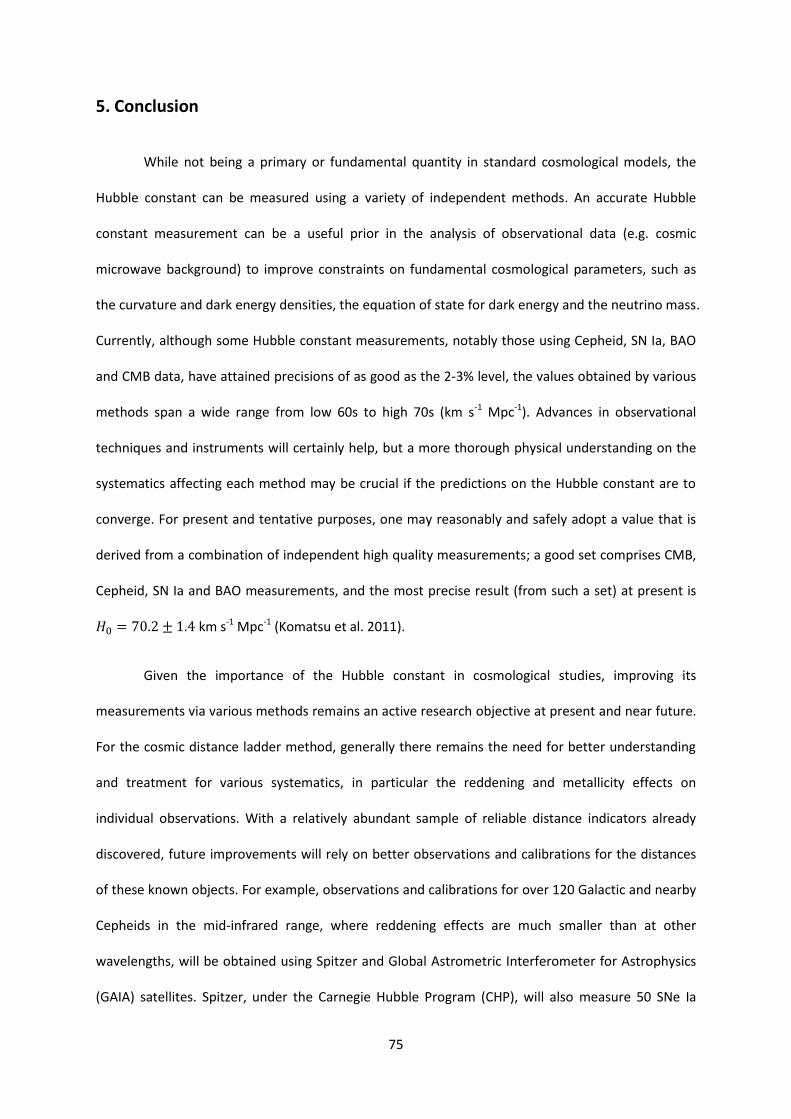
75

5. Conclusion

While not being a primary or fundamental quantity in standard cosmological models, the

Hubble constant can be measured using a variety of independent methods. An accurate Hubble

constant measurement can be a useful prior in the analysis of observational data (e.g. cosmic

microwave background) to improve constraints on fundamental cosmological parameters, such as

the curvature and dark energy densities, the equation of state for dark energy and the neutrino mass.

Currently, although some Hubble constant measurements, notably those using Cepheid, SN Ia, BAO

and CMB data, have attained precisions of as good as the 2-3% level, the values obtained by various

methods span a wide range from low 60s to high 70s (km s-1 Mpc-1). Advances in observational

techniques and instruments will certainly help, but a more thorough physical understanding on the

systematics affecting each method may be crucial if the predictions on the Hubble constant are to

converge. For present and tentative purposes, one may reasonably and safely adopt a value that is

derived from a combination of independent high quality measurements; a good set comprises CMB,

Cepheid, SN Ia and BAO measurements, and the most precise result (from such a set) at present is

km s-1 Mpc-1 (Komatsu et al. 2011).

Given the importance of the Hubble constant in cosmological studies, improving its

measurements via various methods remains an active research objective at present and near future.

For the cosmic distance ladder method, generally there remains the need for better understanding

and treatment for various systematics, in particular the reddening and metallicity effects on

individual observations. With a relatively abundant sample of reliable distance indicators already

discovered, future improvements will rely on better observations and calibrations for the distances

of these known objects. For example, observations and calibrations for over 120 Galactic and nearby

Cepheids in the mid-infrared range, where reddening effects are much smaller than at other

wavelengths, will be obtained using Spitzer and Global Astrometric Interferometer for Astrophysics

(GAIA) satellites. Spitzer, under the Carnegie Hubble Program (CHP), will also measure 50 SNe Ia

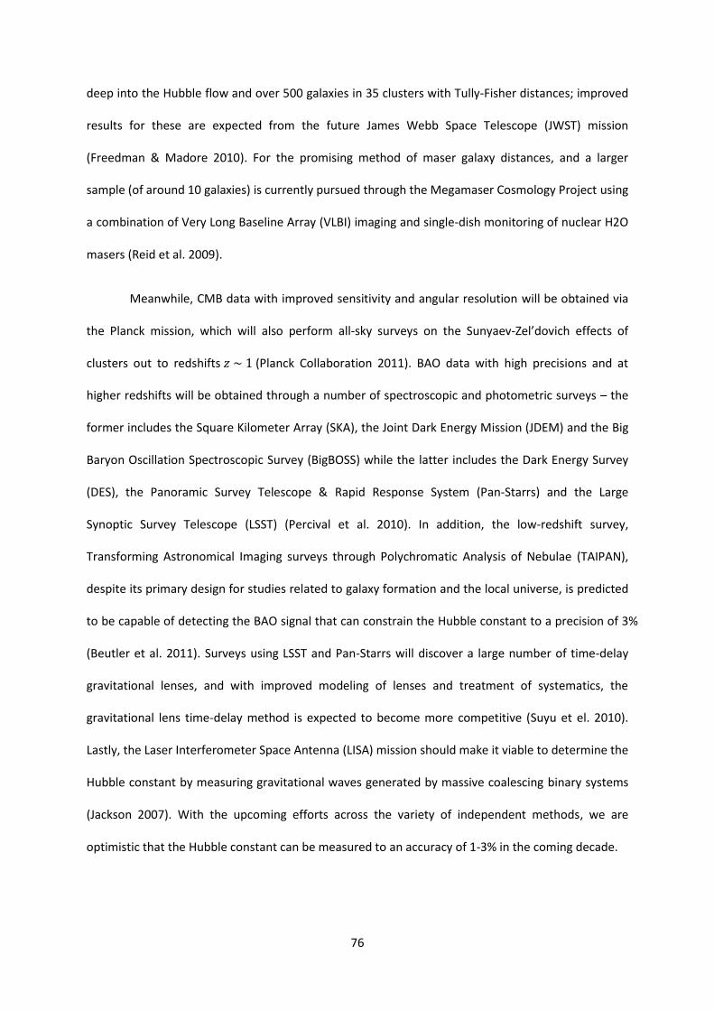
76

deep into the Hubble flow and over 500 galaxies in 35 clusters with Tully-Fisher distances; improved

results for these are expected from the future James Webb Space Telescope (JWST) mission

(Freedman & Madore 2010). For the promising method of maser galaxy distances, and a larger

sample (of around 10 galaxies) is currently pursued through the Megamaser Cosmology Project using

a combination of Very Long Baseline Array (VLBI) imaging and single-dish monitoring of nuclear H2O

masers (Reid et al. 2009).

Meanwhile, CMB data with improved sensitivity and angular resolution will be obtained via

the Planck mission, which will also perform all-sky surveys on the Sunyaev-Zel’dovich effects of

clusters out to redshifts (Planck Collaboration 2011). BAO data with high precisions and at

higher redshifts will be obtained through a number of spectroscopic and photometric surveys – the

former includes the Square Kilometer Array (SKA), the Joint Dark Energy Mission (JDEM) and the Big

Baryon Oscillation Spectroscopic Survey (BigBOSS) while the latter includes the Dark Energy Survey

(DES), the Panoramic Survey Telescope & Rapid Response System (Pan-Starrs) and the Large

Synoptic Survey Telescope (LSST) (Percival et al. 2010). In addition, the low-redshift survey,

Transforming Astronomical Imaging surveys through Polychromatic Analysis of Nebulae (TAIPAN),

despite its primary design for studies related to galaxy formation and the local universe, is predicted

to be capable of detecting the BAO signal that can constrain the Hubble constant to a precision of 3%

(Beutler et al. 2011). Surveys using LSST and Pan-Starrs will discover a large number of time-delay

gravitational lenses, and with improved modeling of lenses and treatment of systematics, the

gravitational lens time-delay method is expected to become more competitive (Suyu et el. 2010).

Lastly, the Laser Interferometer Space Antenna (LISA) mission should make it viable to determine the

Hubble constant by measuring gravitational waves generated by massive coalescing binary systems

(Jackson 2007). With the upcoming efforts across the variety of independent methods, we are

optimistic that the Hubble constant can be measured to an accuracy of 1-3% in the coming decade.

77

Acknowledgements

I would like to thank Dr Carlo Contaldi for his kind advice and generous support throughout

this project, and also for introducing me to the interesting field of Cosmology with his MSc lectures. I

would also like to thank the Physics Department and in particular the Theoretical Physics Group for

the successful organization of the MSc Quantum Fields and Fundamental Forces course, as well as

the College for its comprehensive provision in both academic and non-academic areas. My stay in

London for the past twelve months has been a positive and memorable experience, for which I am

grateful to many who have worked hard to make it possible. Finally, nothing would have been

possible without the ever present and unconditional support from my family, and I would like to

share with them my pride and joy in successfully completing this demanding but rewarding MSc

course.

78

Reference

Alcock C., Paczynski B., 1979, Nature, 281, 358.

Baade W., 1926, Astr. Nachr., 228, 359.

Barnes T.G., Jefferys W.H., Berger J.O., Mueller P.J., Orr K., Rodriguez R., 2003, Ap. J., 592, 539.

Barnes T.G., 2009, In Stellar Pulsation: Challenges for Theory and Observation, edited by J. Guzik and

P. Bradley (In Press), arXiv:astro-ph/0908.3859.

Bassett B. A., Hlozek R., 2009, arXiv:astro-ph/0910.5224.

Beutler F., Blake C., Colless M., Jones D.H., Staveley-Smith L., et al., 2011, MNRAS (Online Early),

arXiv:astro-ph/1106.3366.

Birkinshaw M., 1999, Phys. Rep., 310, 97.

Biscardi I., Raimondo G., Cantiello M., Brocato E., 2008, Ap. J., 678, 168.

Blakeslee J.P., Lucey J.R., Tonry J.L., Hudson M.J., Narayanan V.K., et al., 2002, MNRAS, 330, 443.

Blandford R.D., Narayan R., 1992, Annu. Rev. Astron. Astrophys., 30, 311.

Bonamente M., Joy M.K., LaRoque S.J., Carlstrom J.E., et al., 2006, Ap. J., 647, 25.

Branch D., 1998, Annu. Rev. Astron. Astrophys., 36, 17.

Branch D., van den Bergh S., 1993, Astron. J., 105, 2231.

Carlstrom J.E., Holder G.P., Reese E.D., 2002, Annu. Rev. Astron. Astrophys., 40, 643.

Chernoff D.F., Finn L.S., 1993, Ap. J., 411, L5.

Cox J.P., 1980, Theory of Stellar Pulsation, Princeton University Press: Princeton.

Crotty P., Lesgourges J., Pastor S., 2004, Phys. Rev. D, 69, 3007.

Del Pozzo W., 2011, arXiv:astro-ph/ 1108.1317.

Dodelson S., 2003, Modern Cosmology, Academic Press.

Efstathiou G., Bond J.R., 1999, MNRAS, 304, 75.

Fisher A., Branch D., Hoflich P.A., Khokhlov A., 1995, Ap. J. Lett., 447, L73.

Fixsen D.J., Cheng E.S., Gales J.M., Mather J.C. Shafer R.A., et al., 1996, Ap. J., 473, 576.

Freedman W.L., Madore B.F., Gibson B.K., Ferrarese L., Kelson D.D., et al., 2001, Ap. J., 553, 47.

Freedman W.L., Madore B. F., 2010, Annu. Rev. Astron. Astrophys., 48, 673.

Hannestad S., 2006, Prog. Part. Nuc. Phys., 57, 309.

79

Hillebrandt W., Niemeyer JC., 2000, Annu. Rev. Astron. Astrophys., 38, 191.

Hu W., Sugiyama N., Silk J., 1997, Nature, 386, 37.

Hu W., Dodelson S., 2002, Annu. Rev. Astron. Astrophys., 40, 171.

Hu W., 2005, Observing Dark Energy, 339, 215.

Hubble E.P., 1929, Proc. Natl. Acad. Sci. USA, 15, 168.

Iben I., Renzini A., 1983, Annu. Rev. Astron. Astrophys., 21, 271.

Ichikawa K., Fukugita M., Kawasaki, M., 2005, Phys. Rev. D, 71, 043001.

Jackson N., 2007, Living Reviews in Relativity, 10, 4.

Komatsu E., Dunkley J., Nolta M.R., Bennett C.L., Gold B., et al., 2009, Ap. J. Suppl., 180, 330.

Komatsu E., Smith K.M., Dunkley J., Bennett C.L., Gold B., et al., 2011, Ap. J. Suppl., 192, 18.

Kompaneets A.S., 1956, Zh.E.F.T., 31, 876, Translation (1957) in Sov. Phys. JETP, 4, 730.

Krauss L.M., Chaboyer B., 2003, Science, 299, 65.

Leavitt H.S., 1908, Annals of the Harvard College Observatory, 60, 87.

Leith B.M., Ng S.C.C., Wiltshire D.L., 2008, Ap. J., 672, L91.

Lo K.Y., 2005, Annu. Rev. Astron. Astrophys., 43, 625.

Madore B.F., Freedman W.L., 1991, PASP, 103, 933.

Madore B.F., Steer I.P., 2008, NASA/IPAC Extragalactic Database Master List of Galaxy Distances

(Version Date: 20 Oct 2008), http://ned.ipac.caltech.edu/level5/NED1D/intro.html [Online].

MacLeod C.L., Hogan C.J., 2008, Phys. Rev. D, 77, 043512, arXiv:astro-ph/0712.0618v3.

Moehler S., Bono G., 2008, In White Dwarfs, edited by Burleigh M. and Napiwotski R., Springer-

Verlag, ASSL, arXiv:astro-ph/0806.4456.

Mould J., Sakai S., 2008, Ap. J. Lett., 686, L75.

Mould J., Sakai S., 2009a, Ap. J., 694, 1331.

Mould J., Sakai S., 2009b, Ap. J., 697, 996.

Olling R.P., 2007, MNRAS, 378, 1385.

Percival W.J., Cole S., Eisenstein D.J., et al., 2007, MNRAS, 381, 1053.

Percival W.J., Reid B.A., Eisenstein D.J., Bahcall N.A., Budavari T., et al., 2010, MNRAS, 401, 2148.

Planck Collaboration, 2011, Planck early results VIII: The all-sky early Sunyaev-Zeldovich cluster

sample, arXiv:astro-ph/ 1101.2024v2.

80

Rees M.J., Sciama D.W., 1968, Nature, 217, 511.

Reid M.J., Braatz J.A., Condon J.J., Greenhill L.J., Henkel C., et al., 2009, Ap. J., 695, 287.

Riess A.G., Macri L., Casertano S., Sosey M., Lampeitl H., et al., 2009a, Ap. J., 699, 539.

Riess A.G., Macri L., Li W., Lampeitl H., Casertano S., et al., 2009b, Ap. J. Suppl., 183, 109.

Riess A.G., Macri L., Casertano S., Lampeitl H., Ferguson H.G., et al., 2011, Ap. J., 730, 119.

Rizzi L., Tully R.B., Makarov D., Makarova L., Dolphin A.E., et al., 2007, Ap. J., 661, 81.

Roettiger K., Stone J.M., Mushotzky R.F., 1997, Ap. J., 482, 588.

Rowan-Robinson M., 1985, The Cosmological Distance Ladder: Distance and Time in the Universe,

New York: W.H. Freeman & Co.

Sakai S., Mould J.R., Hughes S.M.G., Huchra J.P., Macri L.M., et al., 2000, Ap. J., 529, 698.

Schechter P.S., 2005, In Gravitational Lensing Impact on Cosmology, edited by Mellier Y. & Meylan G.,

(Cambridge, UK: Cambridge University Press), 225, 281.

Schutz B.F., 1986, Nature, 323, 310.

Seo H.J., Eisenstein D.J., 2007, Ap. J., 665, 14.

Sneden C., Cowan J.J., Beers T.C., Truran J.W., Lawler J.E., et al., 2001, Astrophysical Ages and Times

Scales, 245, 235.

Spergel D.N., Bean R., Dore O., Nolta M.R., Bennett C.L., et al., 2007, Ap. J. Suppl., 170, 377,

arXiv:astro-ph/0603449v2.

Sunyaev R.A., Zel’dovich Y.B., 1970, Comments Astrophys. Space Phys., 2, 66.

Sunyaev R.A., Zel’dovich Y.B., 1972, Comments Astrophys. Space Phys., 4, 173.

Suyu S.H., Marshall P.J., Auger M.W., Hilbert S., Blandford R.D., et al., 2010, Ap.J., 711, 201.

Tammann G.A., 2005, Rev. Mod. Astron., 19, 1, arXiv:astro-ph/0512584v1.

Tammann G.A., Sandage A.R., Reindl B., 2008, Astron. Astrophys. Rev., 15, 289.

Tegmark M., Eisenstein D.J., Strauss M.A., et al., 2006, Phys. Rev. D, 74, 123507.

Tully R.B., Pierce M.J., 2000, Ap. J., 553, 744.

Wesselink A.J., 1946, Bull. Astr. Inst. Netherlands, 10, 91.

Wesselink A.J., 1969, Mon. Not. Royal Astr. Soc., 144, 297.

Wiltshire D. L., 2007, Phys. Rev. Lett., 99, 251101.

Yoshikawa K., Itoh M., Suto Y., 1998, PASJ, 50, 203.