measuring the italian economy. 1300-1861 - paolo malanima · historians will be examined at the...

RIVISTA DI STORIA ECONOMICA, a. XIX, n. 3, dicembre 2003

The work of Seventeenth and Eighteenth centuryarithmetic politicians has recently been resumed. A newinterest has arisen for measuring wealth, income, capitalformation, product, productivity in pre-modern agrarianeconomies. It is now possible for some European regions todraw an outline of per capita product from the Sixteenthcentury onwards and to define an economic hierarchy. 1

Diverse approaches have been tried in these attempts at aquantification. They range from direct case-studies onspecific regions where documents are plentiful and seeminglyreliable (for example contemporary estimates of wealth orincome for taxation purposes) to estimates by contemporarywriters or political men (such as Gregory King’s calculations)and to figures derived from specific kinds of income – mainlywages – (such as the ones advanced by Bairoch some timeago). 2 These attempts have proposed a composite mosaic ofdata with different degrees of reliability.

Our purpose in the following pages is to outline theItalian aggregate and per capita output from the late MiddleAges until the Unification of the country in 1861. TheCentre-North will be considered here as stretching from theSouthern borders of the current regions of Tuscany, Umbria,Marche to the Alps: 161,000 sq. km. Our final series will bemade up of decadal averages from 1300 onwards; as this isthe starting point for our basic statistical data.

A new method will be presented. 3 A series of pastestimates together with values computed by modernhistorians will be examined at the beginning to define thepossible range of the actual variations (par. 1). Four long-term series – population, prices, wages, urbanization – willthen be introduced to obtain a concise view of the product

PAOLO MALANIMA

Measuring the Italian Economy. 1300-1861

266 Paolo Malanima

movement we are looking for and to provide thebackground for statistical elaboration (par. 2). It will thenbe possible from the first three series mentioned to outlinethe trend in agricultural product (par. 3). The next step willbe to add the product of secondary and tertiary sectors tothe agricultural product, indirectly through urbanization, toobtain the long-term estimate we are looking for (par. 4)and to define periodization (par. 5). Once defined, theItalian trend will be compared to the somewhat fragmentedknowledge available for other European regions and to thefew attempts at establishing continuous series for pre-industrial Europe (par. 6).

The method followed here differs from the attemptsmade until now to quantify pre-modern economicmovement. The same method could be usefully employedfor other pre-industrial agrarian economies. The ingredientsneeded to adapt this method to other case-studies aremultisecular series of population, prices (both agriculturaland non-agricultural), wages (possibly, but not necessarily,non-urban, that is agricultural, wages) and series ofurbanization. For Italy these series have only recently beenelaborated. 4 The other data we need are usually available inlate Nineteenth-early Twentieth century modern nationalaccounts.

Absolute certainty in these attempts regarding remote pre-statistical eras is impossible to reach. Reliable results, withnarrow margins of error, are, on the contrary, attainable.After all, in the pre-modern world, changes in consumption,in prices and in product were relatively modest. It is notimpossible to identify the range of variations. Transparency inany step may allow the reader to introduce new data and toobtain better results. We cannot but agree with anexperienced scholar in this kind of research, AngusMaddison, when he writes that «quantification clarifies issueswhich qualitative analysis leaves fuzzy. It is more readilycontestable and likely to be contested. It sharpens scholarlydiscussion, sparks off rival hypotheses, and contributes to thedynamics of the research process». 5

1. Old estimates

The older and more recent attempts may help define therange of possibilities. A simple collection of these calculations

267Measuring the Italian Economy. 1300-1861

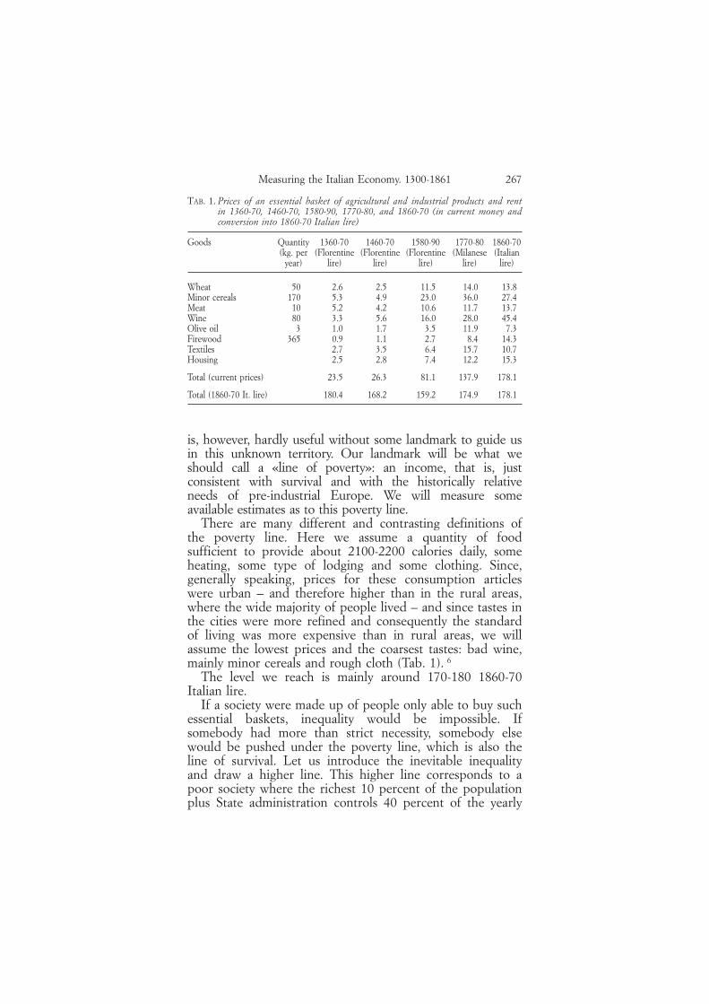
TAB. 1. Prices of an essential basket of agricultural and industrial products and rentin 1360-70, 1460-70, 1580-90, 1770-80, and 1860-70 (in current money andconversion into 1860-70 Italian lire)

Goods Quantity 1360-70 1460-70 1580-90 1770-80 1860-70(kg. per (Florentine (Florentine (Florentine (Milanese (Italian

year) lire) lire) lire) lire) lire)

Wheat 50 2.6 2.5 11.5 14.0 13.8Minor cereals 170 5.3 4.9 23.0 36.0 27.4Meat 10 5.2 4.2 10.6 11.7 13.7Wine 80 3.3 5.6 16.0 28.0 45.4Olive oil 3 1.0 1.7 3.5 11.9 7.3Firewood 365 0.9 1.1 2.7 8.4 14.3Textiles 2.7 3.5 6.4 15.7 10.7Housing 2.5 2.8 7.4 12.2 15.3

Total (current prices) 23.5 26.3 81.1 137.9 178.1

Total (1860-70 It. lire) 180.4 168.2 159.2 174.9 178.1

is, however, hardly useful without some landmark to guide usin this unknown territory. Our landmark will be what weshould call a «line of poverty»: an income, that is, justconsistent with survival and with the historically relativeneeds of pre-industrial Europe. We will measure someavailable estimates as to this poverty line.

There are many different and contrasting definitions ofthe poverty line. Here we assume a quantity of foodsufficient to provide about 2100-2200 calories daily, someheating, some type of lodging and some clothing. Since,generally speaking, prices for these consumption articleswere urban – and therefore higher than in the rural areas,where the wide majority of people lived – and since tastes inthe cities were more refined and consequently the standardof living was more expensive than in rural areas, we willassume the lowest prices and the coarsest tastes: bad wine,mainly minor cereals and rough cloth (Tab. 1). 6

The level we reach is mainly around 170-180 1860-70Italian lire.

If a society were made up of people only able to buy suchessential baskets, inequality would be impossible. Ifsomebody had more than strict necessity, somebody elsewould be pushed under the poverty line, which is also theline of survival. Let us introduce the inevitable inequalityand draw a higher line. This higher line corresponds to apoor society where the richest 10 percent of the populationplus State administration controls 40 percent of the yearly

268 Paolo Malanima

350 lire

262 lire

175 lire1400 1500 1600 1700 1800

1861

1820

1770

1750

1761-70

178017371681

1700

1586-901591

1580-90

1440

FIG. 1. Estimates of per capita GDP (15th-19th c.).

product. This was more or less the rule in past agrariansocieties which were less equalitarian than those in ouradvanced world. 7 The new line is 50 percent higher thanthe physiological minimum just calculated. 8 Another yethigher line is drawn to show a sum twice the line ofpoverty: 350 lire.

We then insert the values available for the six centuriesunder examination into the graph (Fig. 1). 9 These estimatescluster – with only one exception in the Fifteenth century –between the intermediate line of the social minimum andthe highest line which is twice the line of poverty. Theysuggest, for the early Modern Age, a range between 262 and350 1860-70 Italian lire. For the late Middle Ages, the onlyvalue (concerning Tuscany in the first half of the Fifteenthcentury), 10 suggests that per capita income could have beenhigher than in later years.

This first result is quite useful. On its basis, we maysuppose that the variation of per capita product along thecenturies probably moved within a very narrow range. In the140 years from 1861-2000, per capita product increased inItaly 13-14 times – from 1300 International (1990) dollars to18,000. 11 In Central and Northern Italy it increased 16-17times – from 1300-1400 to 23,000. According to this firstprovisional result, based on fragmented and doubtfulevidence, we find that during the 560 years of ourinvestigation, it remained probably between 1200 and 1700-1800 International (1990) dollars. 12 If this were really thecase, ours would appear, if not an «immobile», certainly a«scarcely mobile» history.

The main utility of this first collection of estimates is,anyway, the definition of possible values. Sometimes, whendealing with monetary data processed through price indicesand deflated series, we obtain values that are inconsistent


with past reality. An initial investigation into what people inthe past and recent historians have estimated about thestandard of living and a control of their data by means ofactual prices and quantities may be a starting point toenable us to make more effective comparisons betweenreality and our results. This is only the first step.

2. Four series

Population series, prices, wages and urbanization may benow introduced into this network of possible levels toindirectly outline trends. 13 This is the second step.

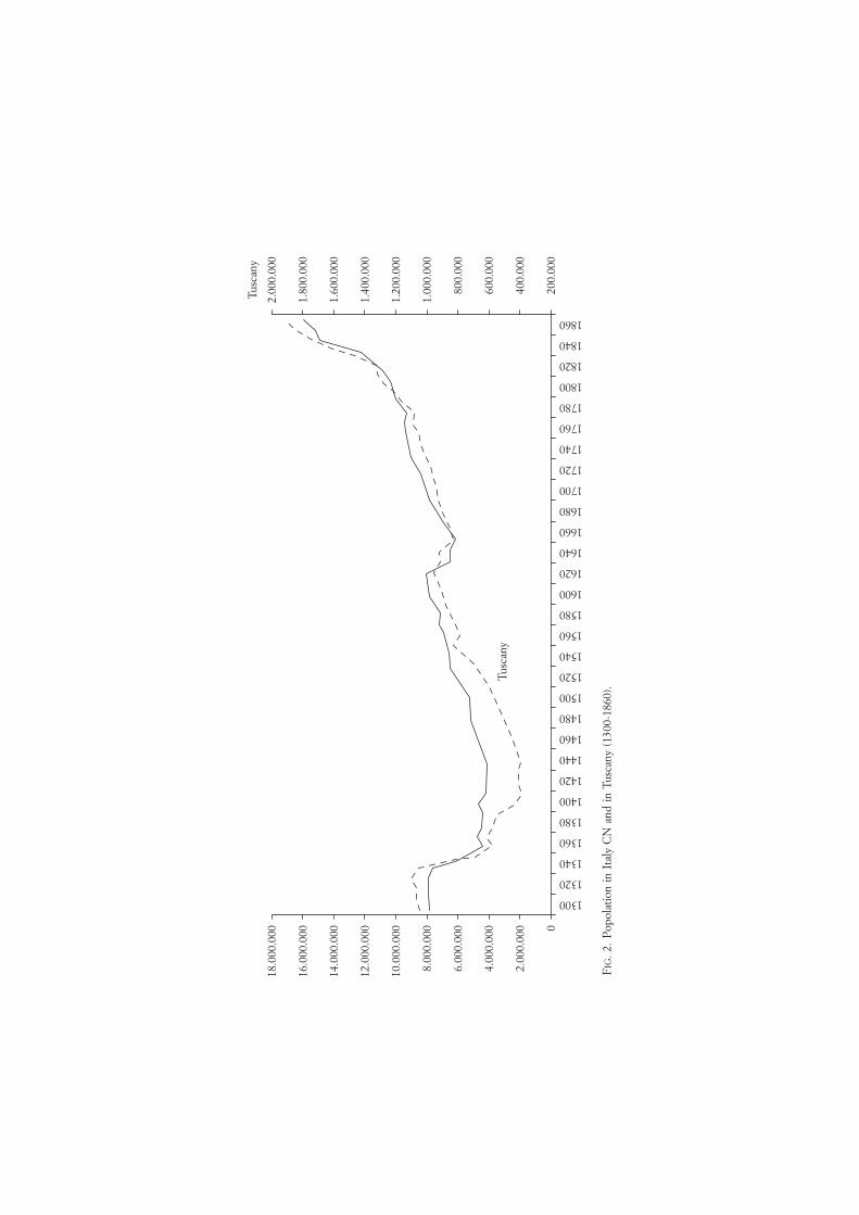
Population. Italy’s population has been partiallyreconstructed through the aggregate method of inverseprojection: from 1575 the demographic movement inTuscany; 14 from 1650 in the Centre-North. 15 Especially forTuscany, the result describes a more satisfying long-termtrend than the ones already available. For Central-NorthernItaly as a whole, the trend is more uncertain than forTuscany. For the period before the Sixteenth century, Italy’spopulation movement is still based on the reconstruction ofKarl Julius Beloch. 16 More recent results confirm Beloch’strend. 17 Here decadal values are interpolated from Beloch’sfigures and from the ones proposed by more recentdemographers (Fig. 2). In particular, the late-medieval levelcould be better specified. 18

The existing differences between Tuscany, on the onehand, and the Centre-North, on the other, are easilyexplainable: in the middle of the Fourteenth century, theBlack Death was less deadly in the Po Valley than in thedensely populated and highly urbanized Tuscany. In the1629-30 epidemics, mortality was, on the other hand, muchhigher in Lombardy and Venetia than in Tuscany. After themiddle of the Seventeenth century the intensity of thepopulation rise was the same in Tuscany and Po Valley.

From a demographic viewpoint, the beginning of theFourteenth century brought in a new era. The late medievalincrease was over. A long period – about 300 years – ofstability and decline was just starting. In particular, the twomajor plague epidemics, in 1348-49 and in 1629-30, togetherwith other minor, but frequent epidemics, contributed to haltthe rising trend. The two main plague outbursts were

270 Paolo Malanima

18.0

00.0

00

16.0

00.0

00

14.0

00.0

00

12.0

00.0

00

10.0

00.0

00

8.00

0.00

0

6.00

0.00

0

4.00

0.00

0

2.00

0.00

0 0

2.00

0.00

0

1.80

0.00

0

1.60

0.00

0

1.40

0.00

0

1.20

0.00

0

1.00

0.00

0

800.

000

600.

000

400.

000

200.

000

Tusc

any

1300

1320

1340

1360

1380

1400

1420

1440

1460

1480

1500

1520

1540

1560

1580

1600

1620

1640

1680

1700

1720

1740

1760

1780

1800

1820

1840

1860

1660

Tusc

any

FIG

. 2.

Pop

olat

ion

in I

taly

CN

and

in T

usca

ny (

1300

-186

0).


separated by a relatively rapid increase from 1450 until about1575 19 and then a decline. In the middle of the Seventeenthcentury, the population of Central-Northern Italy was 1.5million lower than at the peak of the medieval rise. Themodern growth of the population began around 1660-70. Itwas a European and probably a worldwide demographicchange. In Central-Northern Italy the population was6,230,000 in 1650. It was more than 10 million in 1800; itwas 16 million in 1860-70.

Italian demographic trends from the late Middle Agesmay thus be divided into two 300-350 year phases: one ofrelative stability, from 1300 until 1650; and one of rapidincrease from 1650 until about 2000.

Prices. Changes in prices were very slow before theTwentieth century; in consumption patterns they werealmost non-existent. Prices increased in Italy by less than0.5 percent a year in the 560 years from 1300 to 1860-70. Inconsumption, the only meaningful transformations inCavour’s time, compared to Dante’s era – and probably evento Virgil’s time – were maize and potato, tomato, coffee,tobacco, all introduced in the Sixteenth and Seventeenthcenturies. With the exception of maize, they hardly modifiedthe Italian consumption standards. 20

The price index presented here closely follows thedemographic movement from the late Middle Ages until theend of the Nineteenth century (Fig. 3). 21 Certainly, otherfactors also influenced price trends, first and foremost theavailability of precious metals and monetary exchange.However, their importance was, generally speaking,secondary. Prices increased in the late Middle Ages, whenthe population rose; they decreased and stabilized for acentury after the Black Death, they rose with the Sixteenth-century population growth; they decreased after the 1575epidemics and especially after the 1629-30 plague; theyincreased again at the end of the Seventeenth century. Achange in this correlation took place only after 1820: pricesbecame relatively stable while the population increased. Wewill return to this significant new trend later. A growingpopulation in this pre-modern world implied an increase inthe demand for primary articles, an increase in the velocityof money circulation and often an increase in money stockin the face of a slowly growing supply of agricultural goods.Prices could only rise.

272 Paolo Malanima

120

100

80

60

40

20

0

1840

-50

1300

-10

1330

-40

1360

-70

1390

-00

1420

-30

1450

-60

1480

-90

1510

-20

1540

-50

1570

-80

1600

-10

1630

-40

1660

-70

1690

-00

1720

-30

1750

-60

1780

-90

1810

-20

FIG. 3. Italian price index (1300-1870) (1420-40 = 1).

Since the method of estimating agricultural productinvolves the use of agricultural and non-agricultural prices,we need to distinguish their trends. 22 Agricultural goodsincreased much more than non-agricultural ones and morethan the price index: by 9.20, 2.31 and 8.24 respectivelyfrom 1420-40 until 1860-70. While decreasing returnsfollowing demographic increases characterized agriculture,in industry and services we find increasing returns from theincreasing cooperation and accumulation of knowledge. Butsince food and materials increased in price, non-agriculturalprices inevitably followed suit. The classical and especiallyRicardian explanation about the relation between agricultureand industry fits the pre-industrial world well.

Wages. Urban wage rates steadily declined from the lateMiddle Ages. 23 Their movement shows a clear inverserelation both as regards prices and the population. Fromtheir zenith in the Fifteenth century to their nadir between1800 and 1870 they decreased more than 50 percent in realterms (Fig. 4). 24 Their decline occurred not only in relationto the Fifteenth century, a happy period for salariedworkers, but also to the Fourteenth century. Since, as weshall see, per capita output performance was much lessnegative, the only explanation is that workers worked muchless when wages were high and were obliged, instead, to toilmuch more when wages were low. The ratio between wage


120

100

80

60

40

20

0

1285

-95

1320

-30

1340

-50

1360

-70

1380

-90

1400

-10

1420

-30

1440

-50

1460

-70

1480

-90

1500

-10

1520

-30

1540

-50

1560

-70

1580

-90

1600

-10

1620

-30

1640

-50

1660

-70

1680

-90

1700

-10

1720

-30

1740

-50

1760

-70

1780

-90

1800

-10

1820

-30

1840

-50

FIG. 4. Builders’ wages in Tuscany (1285-1860) (1420-40 = 1).

level and work supply, which is direct today, was inverse intraditional agrarian society. We know very little, at themoment, about real labour earnings. A complete pictureshould include figures on the working population over timeand working hours; topics on which information is stillscant and unsatisfactory.

Some clear phases are discernible in the declining trend.A strong rise took place after the Black Death and the latemedieval epidemics and lasted until population growthresumed around 1450. Real wage rates rapidly diminished inItaly thereafter; much earlier than in other Europeanregions. They remained low until the Seventeenth centurydemographic decline, and rose thereafter. A sharp and rapiddecline occurred in the Eighteenth century. The lowest levelwas reached between 1810 and 1820. A very uncertainrecovery took place after 1820. On the eve of the FirstWorld War, however, Italian wages were still lower than inthe late Middle Ages.

Agricultural wages follow the same long-run trends,although the long-term decline was stronger (Fig. 5). 25 Theywere higher in relation to urban wages in periods of urbandifficulty and crisis as during the late Middle Ages, whenmarkets for Italian products and services plummetedbecause of the decline in the population, and during thefirst half of the Seventeenth century, another well-known eraof crisis for Italy’s urban society.

274 Paolo Malanima

Urbanization. Urbanization trends always provideimportant information about the health of the economy inthe pre-industrial world. 26 An increase in the urbanpopulation is a symptom of change in the economicstructure in favour of the secondary and tertiary sectors,which usually are more productive and innovative than theprimary. On the other hand, agriculture too has to be moreproductive in a highly urbanized system, since fewerworkers in the countryside have to feed a higher number ofurban inhabitants.

If a relation exists between urbanization and economicperformance, then Central-Northern Italy reveals a decliningtrend in productivity since the movement is clearlydownward oriented: from 1300 until 1861 the decline inurbanization was 5 percent if we consider the centres withmore than 5000 inhabitants (Fig. 6 and Tab. 2). 27 The fallwas sudden and sharp during the late medieval industrialand commercial crisis; recovery, however, was rapid in thesecond half of the Fifteenth century. A slow downwardmovement took place from the Seventeenth century; in thefirst half of the Nineteenth century the decline quickenedjust when urban populations were increasing in relativeterms all over Europe. Italy was, therefore, the onlyexception, as far as we know, in an urbanizing continent. 28

FIG. 5. Agricultural wages in Central-Northern Italy (1320-1860).

120

100

80

60

40

20

0

1300

-10

1320

-30

1340

-50

1360

-70

1380

-90

1400

-10

1420

-30

1440

-50

1460

-70

1480

-90

1500

-10

1520

-30

1540

-50

1560

-70

1580

-90

1600

-10

1620

-30

1640

-50

1660

-70

1680

-90

1700

-10

1720

-30

1740

-50

1760

-70

1780

-90

1800

-10

1820

-30

1840

-50


50

40

30

20

10

0

1000

1200

1300

1400

1500

1600

1700

1800

1901

1951

FIG. 6. Urbanization in Italy CN (1000-1950).

TAB. 2. Urbanization in Central-Northern Italy from 1300 to 1861 (cities with atleast 5000 inhabitants)

Urban Urbanizationpopulation %

1300 1,657 21.41350 992 17.71400 829 17.61450 752 17.01500 1,117 21.01550 1,357 20.01600 1,438 18.41650 947 15.21700 1,363 16.91750 1,646 17.71800 1,788 17.51861 2,590 16.2

An initial reconstruction. The four previous series allow usto make an initial reconstruction of Italian economicperformance over six centuries.

As regards the aggregate trend, while in the first threecenturies of our reconstruction, we can expect stability and,in some periods, a decline in aggregate output, because ofthe overall stability (with periods of decline) in population,in the period 1650-1861, growth must have taken place.Such a long-lasting demographic rise must have beensustained by an increase in output.

Per capita production trends must have been different. A

276 Paolo Malanima

long-run increase in the population and in prices and adecline in wage rates and urbanization imply a decrease inproductivity and, as a consequence, a decrease in per capitaoutput if the employment structure does not drasticallychange. While in late medieval and early modern eras, theplague kept the population level low, the pressure onresources increased thereafter. Decreasing returns must havebeen followed by a fall in per capita income.

The ratio between natural resources and humansinevitably declines when the population rises. Relativescarcity of natural resources may be compensated by anincrease in produced resources, that is in capital, by meansof new investments. If the rate of increase in capital ishigher than the rate of increase in manpower, that is to say,in the population, productivity can grow and per capitaproduct can grow as well. Due to the increase in capital,labour demand is higher than labour supply and wage rateshave to rise in real terms together with the population andprices. We can suppose, on the contrary, that in Italypopulation growth was not followed by a more rapidincrease in capital formation (especially in machinery andmechanical power). A long-term population rise must havebeen followed by a fall in the marginal product of labourand hence in the per capita product (when the activity rateremains unchanged), as wage rates clearly reveal. While inthe first long period up to 1650 the plague heavilycountered this tendency, keeping population consistent withnatural and produced resources, from the late Seventeenthcentury the rise in population was no longer met by suchhigh rates of recurring mortality. As a consequence,productivity and per capita product must have declined.The stop to the negative trend of real wages from 1820,together with price stability and a sharp rise in thepopulation, implies, on the contrary, a break in the decline,even though the slow but continuous fall in urbanizationsuggests that the downward trend had not been completelyreversed. The decline had only been temporarily halted. Theforces of growth, however, were not yet fully at work. A lowprofile equilibrium still prevailed.

The results of the previous series do not seem easy to puttogether without the means of this classical theoreticalapparatus.


3. Agricultural product

Since, for this prestatistical world, we lack sufficient andreliable data on the supply side, we can try to reach ourgoal of arriving at a concise view of Italian agriculturalperformance from the demand side. 29 Agricultural grossoutput could be simply calculated as the result of theproduct of per capita agricultural consumption – which isrelatively well known – by the population. The use of thisvery simple method 30 depends, however, on twoassumptions:

1) the economy must be closed, that is without exportsand imports of agricultural products from and towardsother regions. Only in this way do consumption andproduction coincide;

2) everybody must consume the same value ofagricultural goods without changes brought on bymovements in prices and incomes.

With regard to the first assumption, internal consumptionis equal to internal product only if exchanges do not existbetween our economy and the outside world. We know,however, that Central-Northern Italy was not isolated froman agricultural viewpoint. The densely populated cities inthe Centre and North imported wheat, oil, wine from theSouth and from non-Italian regions as well, already in thelate Middle Ages. Considerable imports of raw materials –silk, wool especially – took place in several periods. From aquantitative viewpoint, however, their importance was not sosignificant. In a period of intense importation of agriculturalgoods, like the second half of the Sixteenth century, theyaccounted for less than 5 percent of the Centre-North’sgross product. 31 From the Seventeenth century onwards,agricultural raw materials such as raw silk began to beexported from the North beyond the Alps and, as aconsequence, to counterbalance agricultural importsespecially from Southern Italy.

Since, on the whole, the value of imports and exports inthe period 1300-1861 – which are in any case hard toquantify exactly – were never high enough to modify thesubstance of our calculations, it is preferable to ignorethem. 32

The situation is different in the case of the secondassumption. The movement of prices and real incomeheavily influenced the consumption of agricultural goods.

278 Paolo Malanima

2,0

1,8

1,6

1,4

1,2

1,0

0,8

0,6

0,4

0,2

0

1300

-10

1330

-40

1360

-70

1390

-00

1420

-30

1450

-60

1480

-90

1510

-20

1540

-50

1570

-80

1600

-10

1630

-40

1660

-70

1690

-00

1720

-30

1750

-60

1780

-90

1810

-20

1840

-50

FIG. 7. Per c. agricultural consumption (1300-1860) (1860-70 = 1; different elasti-cities).

We can not keep consumption unchanged. If we wish todefine agricultural product from the demand side, we haveto take these conjunctural changes into account. Anelasticity coefficient for prices and income is the result ofthe ratio between a change in the quantity demanded and achange in prices or income or in both. Now, since we arelooking for changes in quantity over the centuries, butknow, more or less, which coefficients of elasticity areconsistent with the economy we are studying and knowabout prices and wages, we can proceed from elasticitycoefficients for prices and wages to estimate changes inagricultural quantities. 33 This method of estimatingagricultural product from the demand side has a traditionespecially in studies on England and may produce goodresults. 34

The problem now is what coefficients to use. We can takethe ones worked out for today’s backward economies. Firstof all, we take the four pairs of wage and price coefficientsusually employed in such studies. Since the absolute sum ofboth coefficients must be 1, the combinations of the 8 mostfrequently used values as price and wage coefficients areonly 4. As we can see, if price and wage series do not movefar from the chosen benchmark, the results we reach aresimilar (Fig. 7). Only for the Fifteenth century, when bothprices and wages are relatively far from the basis of ourindices, do results diverge widely. In a dynamic economy


120

100

80

60

40

20

0

1300

-10

1330

-40

1360

-70

1390

-00

1420

-30

1450

-60

1480

-90

1510

-20

1540

-50

1570

-80

1600

-10

1630

-40

1660

-70

1690

-00

1720

-30

1750

-60

1780

-90

1810

-20

1840

-50

FIG. 8. Gross agricultural product in Italy CN (1300-1870) (1860-70 = 100).

experiencing great changes in the level of per capitaagricultural production over time, the method could resultin curves that diverge too much. Fortunately this is not thecase with Italy.

In the end we have chosen an 0.4 wage elasticity and a –0.6elasticity for agricultural prices. The use of other coefficientsmight introduce only marginal variations in our results. Thewage series is an average made up of urban and rural wagesand not just a series of urban wages, which is usuallyemployed due to the lack of agricultural wage series formany other regions in Europe. Estimates concern changes inquantity consumed – and hence in product – over thecenturies. 35 Assuming a real value for per capita agriculturaloutput in 1860-70 from the results of the newly revisedversion of the Italian national accounts, we may construct along-term series. 36 Multiplying the series by the population,we can estimate gross agricultural product.

The gross product series is inevitably rising, as weexpected, because of the demographic growth. It fallssharply in periods of population decline. It declined, thoughslightly, in the second half of the Eighteenth century, whilethe population was increasing (Fig. 8).

Per capita agricultural product falls over the centuries. 37

However the decline was halted when epidemics determinedsharp demographic trend reversals, especially during thecentury 1350-1450 and after 1629-30. As we see, the lowest

280 Paolo Malanima

level was reached in the second decade of the Nineteenthcentury. Afterwards there was a slight recovery and then aperiod of stability. No growth at all took place in Italy at thebeginning of Modern European Growth, although thedemographic rise was not followed by a decline in percapita product as had always happened before. From aclassical perspective, we might suspect that capital formation– especially for agricultural equipment – was then increasingat the same rate as the population.

4. Industry and services

Urbanization would suggest that in Northern and CentralItaly the typical urban occupations, that is, those pertainingto industry and services, declined in the centuries we areconsidering, although, as we have seen, with occasionalperiods of recovery. In the economic structure, industry,trade, banking and other services played a central role at thebeginning of the Fourteenth century. This was no longer thecase in the period of Unification. In comparison with otherEuropean regions, at that time Italy appeared to be adeurbanized or scarcely urbanized country. The conclusionshould be that the Italian economic structure was moreadvanced – that is less agrarian – in the Fourteenth centurythan at the end of the Nineteenth.

We should bear in mind, however, that all over European increasing dispersion of industrial and commercialactivities in the countryside took place from the Seventeenthcentury on. Protoindustry was in fact characterized by thebirth of secondary activities outside the towns. Commercialnetworks developed in the countryside all over thecontinent. We might suspect, then, that while in the earlyModern Age urbanization was declining in Italy, industrialdispersion in the countryside was counterbalancing urbandecline and that, in the end, secondary and tertiary sectorsflourished in both the Eighteenth and Nineteenth centuriesdespite deurbanization. We know, however, that because ofthe intensity of agricultural labour among peasant families,(as a consequence of the manifold cultivations – wheat butalso maize – and especially of trees – vineyards andmulberry trees) that characterized Italian agriculture,protoindustrial activities did not play such an important rolein Italy as in Northern European regions. 38 Wool, cotton,


silk and straw industries certainly advanced in small centresin the countryside. Overall, however, they do not seem tohave compensated for the relative decline in the cities. Thesilk industry was the most important secondary sector in theNorth Italian countryside. On the eve of Unification,however, only about 200,000 workers were employed inprocessing raw silk; many more were engaged in breedingsilkworms and in mulberry tree cultivation (but these wereagricultural and not industrial occupations).

In order to quantify the role of secondary and tertiaryactivities in Italy, we will now identify the relationshipbetween urbanization and the weight of the secondary andtertiary sectors on GDP after Unification, for which directstatistical data are available. If we take the relationshipbetween urbanization and secondary and tertiary sectors inthe period between Unification and the Second World War,we may then use the resulting equation to assess theimportance of these sectors in previous centuries. In thisway, we avoid the problem of secondary activities outsidethe cities. We do not identify, in fact, cities with industryand trades as we would do if we took the urban populationas being made up of workers in secondary and tertiaryactivities. We simply discover the relationship betweenurbanization on the one hand and the product fromindustry and services on the other; whether the productfrom these two sectors was created within the city walls oroutside. In the period from 1861 until 1938 non-urbanindustrial occupations flourished in Italy and our regressionis based on urbanization – the dependent variable – andsecondary and tertiary sectors – the independent variable –,widespread in the countryside as well and not only in thecities.

Both urbanization after 1861 and the economic structureare imperfectly known. Data on urban centres stoppedbeing recorded after the 1871 census and demographers andstatisticians have only been able to work out series of datathat are not wholly comparable to those for the previouscenturies. As to the economic structure, only uncertain dataare available as the differences among the diverse seriesworked out by various historians reveal. Fortunately therecent publication of the first results of the revised nationalaccounts at least throws light on the years 1891, 1911 and1938. We have taken these three years as our benchmarks.The complete reconstruction of industrial output from 1861

282 Paolo Malanima

TAB. 3. Urbanization in Italy and the share of secondary and tertiary production inGDP 1861-1938

Urbanization II and III sectors on GDP

1861 16.2 45.51871 17.8 45.41881 19.6 52.01891 20.7 55.71901 23.2 56.31911 25.9 61.91921 26.6 62.11931 29.0 66.01938 29.3 72.1

TAB. 4. Estimated proportions of GDP in Italy CN by sectors of origin 1330-1861(percent)

I II and III

1300 45 551350 48 521400 55 451450 54 461500 46 541550 48 521600 51 491650 57 431700 54 461750 52 481800 53 471861 53 47

until 1913 helps clarify the movement of a part of non-agricultural product. The series for urbanization and GDPstructure are based on the least doubtful among theavailable data (Tab. 3). 39 The regression of urbanization inrelation to the economy is significant from a statisticalviewpoint (Fig. 9). 40

We can now use the equation to estimate the weight ofsecondary and tertiary activities from urbanization.

The economic structure from the late Middle Ages toUnification does not show profound changes like those wewould probably find in other expanding North-Europeaneconomies (Tab. 4). 41 The weight of agriculture remainedbetween 45 and 55 percent. 42 It is impossible to distinguishthe relative weight of industry and services. From theevidence after Unification, we suspect that non-agriculturaloutput was equally divided between them.


35

30

25

20

15

1010 20 30 40 50 60 70 80

y = 0,5199x –6,7266R2 = 0,9454

FIG. 9. Urbanization and II and III sectors on GDP.

In the late Middle Ages the Italian economy was, inrelative terms, more industrialized than in the mid-Nineteenth century. The presence of services was higher.The arrival of the Black Death, which throughout Europereduced the number of customers for the Italian secondaryand tertiary sectors, led to a decline in urbanization and inthe role of non-agricultural occupations, although thedecline in urban occupations was compensated for by theexpansion of demand for rural labour which was muchmore productive than before and therefore expensive. Wagerates increased, especially in the countryside. The samelevels of per capita product were attained in the Fourteenthand Fifteenth centuries through two very different economicstructures. After a secular recovery in the Sixteenth century,from the Seventeenth the weight of agriculture rose beyond50 percent and remained there until the end of theNineteenth century. As far as we can see, the variations overtime were, generally speaking, relatively weak in the matureItalian agrarian economy.

5. Trends

Trends for per capita product (Fig. 10) do not contradictthe evidence we find in the literature on the subject or inthe already-examined series.

From the late Middle Ages to the end of the Nineteenthcentury a considerable growth took place in aggregate

284 Paolo Malanima

500

450

400

350

300

250

200

150

100

50

0

1300

-10

1340

-50

1380

-90

1420

-30

1460

-70

1500

-10

1540

-50

1580

-90

1620

-30

1660

-70

1700

-10

1740

-50

1780

-90

1820

-30

1860

-70

FIG. 10. Per c. GDP in Italy CN 1300-1870 (agricultural-low-and total).

terms. The Northern and Central Italian economy wasalways able to produce more for the increasing population.This growth was financed primarily by a decline in thestandard of living (Fig. 11). Per capita income fellcontinuously and particularly after the population rise whichbegan in the second half of the Seventeenth century. Itreached a very low level in the first two decades of theNineteenth century and more or less maintained such a lowlevel up to the start of Modern Growth at the very end ofthe Nineteenth century. 43

As we can see, per capita product remained, in the earlyModern Age, just within the range identified bycontemporaries and by historians in their attempts at aquantification: around 260-350 1860-70 Italian lire. 44 In thelate Middle Ages it often exceeded the highest level of 350lire. Our results are consistent with the already mentionedolder and more recent attempts at quantification. Theyallow us to identify a long-term trend amidst the variety ofdifferent values.

Considering per capita output, we may thereforedistinguish:

– the golden age: from the prosperous late Middle Agesto the end of the Sixteenth century when per capita productwas around 400 Italian 1860-70 lire;

– the silver age: from the end of the Sixteenth century to1730-40 when per capita product was around 350 Italian1860-70 lire;


FIG

. 11.

GD

P a

nd p

er c

. GD

P in

Ita

ly C

N (

1300

-187

0).

500

450

400

350

300

250

200

150

100 50 0

5.00

0.00

0

4.50

0.00

0

4.00

0.00

0

3.50

0.00

0

3.00

0.00

0

2.50

0.00

0

2.00

0.00

0

1.50

0.00

0

1.00

0.00

0

500.

000 0

Per

c. G

DP

GD

P

1300-10

1330-40

1420-30

1540-50

1660-70

1780-90

1360-70

1390-00

1450-60

1480-90

1510-20

1570-80

1600-10

1630-40

1690-00

1720-30

1750-60

1810-20

1840-50

286 Paolo Malanima

– the iron age: from 1730-40 to the start of ModernGrowth, at the end of the Nineteenth century, when percapita product was about 300 Italian 1860-70 lire.

In our developed world, we have been used to thinkingthat per capita and gross product move in the samedirection, albeit with different speeds. This has been thecase since the start of Modern Growth. It was not so before:often, when gross product increased, per capita product fell.

We have also been used to thinking that from the lateMiddle Ages to the present the European economy hasmoved in the direction of progress. The path followed byItaly shows that, at least in one case, this was not so: longdecline and not long progress characterized its economy for6 centuries.

6. On the European background

Data on per capita GDP have been proposed for otherEuropean countries in the early Modern Age. Needless tosay, the degree of uncertainty is still high. At the moment,only the size may be defined and with several reservations.From the figures collected for some regions, we might drawan initial conclusion that from 1500 until 1800 per capitaproduct probably moved mainly 45 in the range of 1000-2000international (1990) dollars and that the economies did notdiverge much. Usually not more than a 20-30 percentdifference existed between the best and the worstperformer. 46 Things changed in the age of Modern Growth.

Much more uncertain is the relative position of eachEuropean economy. For the United Kingdom and theNetherlands, we have more reliable estimates to compare toItalian estimates than for other European countries (Tab. 5). 47

We will start with the relative position of several WesternEuropean countries in the second half of the Nineteenthcentury and go backwards.

In 1870 some regions exceeded the level of 2000International 1990 dollars and United Kingdom was at 3200.Italy was relatively backward with less than 1300 dollars. 48 Alittle higher was the position of the Central and Northernregions, with 1400 dollars. In 1820 the Netherlands and theUnited Kingdom were the most advanced countries. 49 Thedistance from the rest of the Western European regions suchas Belgium, France, Italy, Denmark, Switzerland, Sweden


TAB. 5. Per capita product in United Kingdom, the Netherlands and Italy CN. 1700-1870 (International 1990 $ PPP)

UK The Netherlands Italy CN

1700 1250 2100 14401750 1500 2000 15701800 1580 1800 13401820 1700 1820 13601870 3200 2750 1400

(probably Germany), was, however, only 25-30 percent. Italyshared the relative retardation of many followers in a difficultmoment for the economies of the whole continent.

During the first part of the Eighteenth century Italy wasprobably second behind the Netherlands and on a par withthe United Kingdom, 50 losing ground only in the secondhalf of the century. Relative levels were not so different inthe preceding century, but while the rise in per capitaincome in the Seventeenth century Italy had been the effectof the decrease in population, in the Netherlands and inBritain it had been pushed forward by the increase in theproduct. In the ratio between gross product and population,a fall in the denominator had taken place in Italy, while inthe Netherlands and in Britain the numerator had risen.

For the late medieval and early modern ages, the data onper capita product are not well grounded. Sometimesexcessively low figures have been suggested, which arehardly consistent with population survival. 51 Our «povertyline» presented at the beginning shows that 800 1990International dollars was, in pre-modern times, hardlyconsistent with survival (and without inequality). Areconstruction of agricultural per capita product from wagesand prices for several European countries suggests a rangeof 600-1000 dollars in the centuries between 1300 and1600. 52 If we assume that agriculture accounted for 50-60percent of gross product, then per capita product had to beat least in the range of 1000-1600 International 1990 dollars:a range consistent with our series.

According to our results, Italy would have been well inthe forefront of this hierarchy and perhaps would haveoccupied first place in the late Middle Ages. Italy was atthat time a mature economy: an economy near theproduction possibilities frontier. It lost increasingly moreground during the early Modern Age both in relative and

288 Paolo Malanima

absolute terms. While its economy as a whole grew, its levelof per capita product fell.

Italy completely missed the First Industrial Revolution,the age of coal, iron and mixed farming. It was impossibleto adapt the English model to the available naturalresources. The lack of coal, the scarcity of iron and the drysoils of the peninsula, with the only exception of part of thePo Valley, was thus an obstacle too difficult to overcomeconsidering the technological level of the time. The relativebackwardness of the peninsula grew during the Nineteenthcentury. From the late Middle Ages to the end of theNineteenth century Italy followed the downward curve froma condition of progress to a state of backwardness.

While Italy missed the opportunities of the first wave ofModern Growth, it was able, on the other hand, to exploitthe possibilities offered by the Second Industrial Revolution,the age of oil, electricity, chemical fertilizers, whoseinception was at the very end of the Nineteenth century. Itbecame possible to import what Italy was lacking (fossilenergy sources and agricultural products), to exploit whatwas available (energy from waterfalls) and to export, thanksto emigration, what Italy had in abundance: people.

7. Conclusions

We sum up now the least uncertain points:1) in the long period from 1300 to 1860, per capita

product remained in Central-Northern Italy within the narrowrange of between 1300 and 1900 international 1990 dollars;

2) during the six centuries, the trend of per capita outputdeclined, while gross product rose;

3) the relative importance of non-agricultural sectorsdiminished from the late Middle Ages on (with a shortrecovery in the Sixteenth century);

4) especially around the mid-Eighteenth century, theItalian economy shifted towards the lower margin of thenarrow range of the European per capita product andstayed there until the start of Modern Growth;

5) compared to other Western European regions, theItalian economy was developed in the late Middle Ages; itwas still advanced in the early Modern Age up to the mid-Eighteenth century; it was backward from then until the endof the Nineteenth century.


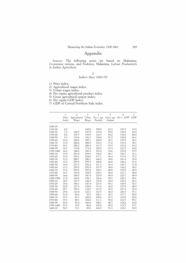
Appendix

Sources: The following series are based on Malanima,L’economia italiana, and Federico, Malanima, Labour Productivityin Italian Agriculture.

IIndices (base 1860-70)

1) Price index;2) Agricultural wages index;3) Urban wages index;4) Per capita agricultural product index;5) Gross agricultural output index;6) Per capita GDP index;7) GDP of Central-Northern Italy index.

1 2 3 4 5 6 7Price Agricultural Urban Per c. agr. Gross agr. Per c. GDP GDPIndex Wages Wages Product Output

1300-101310-20 6.2 162.0 128.0 63.2 147.9 74.31320-30 7.2 142.5 147.0 119.6 59.0 138.2 69.41330-40 8.2 125.5 130.9 116.3 58.2 134.4 68.41340-50 9.3 110.6 126.7 118.8 57.2 130.8 64.11350-60 12.4 180.6 189.1 128.8 45.1 135.5 48.31360-70 11.0 204.6 206.9 132.2 37.2 133.2 38.11370-80 10.1 282.2 280.4 111.5 33.5 112.4 34.31380-90 16.3 174.8 173.4 120.5 33.9 121.5 34.81390-1400 16.2 188.2 185.4 123.0 34.6 123.8 35.51400-10 13.0 241.4 239.6 136.0 40.1 136.7 41.11410-20 13.2 239.1 238.6 137.1 36.4 137.6 37.21420-30 11.2 280.7 280.1 146.9 38.6 147.4 39.41430-40 13.2 259.5 255.5 140.0 36.8 140.6 37.61440-50 14.4 237.5 236.4 137.1 36.4 136.7 37.01450-60 13.2 259.5 252.9 137.5 38.0 136.2 38.31460-70 13.2 259.5 253.8 138.1 40.8 135.8 40.91470-80 14.1 195.0 198.0 129.3 40.0 127.1 40.01480-90 14.6 188.5 187.4 125.8 40.9 123.7 40.91490-1500 17.2 160.4 156.7 116.6 38.3 120.1 40.11500-10 18.5 147.5 142.9 115.8 38.4 125.2 42.31510-20 15.6 186.1 187.4 127.4 45.1 144.9 52.31520-30 22.8 127.4 128.6 111.6 42.2 127.0 48.91530-40 25.7 109.1 118.5 111.9 45.2 127.4 52.41540-50 25.6 114.4 122.1 112.5 46.4 126.3 53.11550-60 31.8 83.6 92.5 106.3 45.1 117.7 50.81560-70 33.3 87.3 100.6 109.6 47.3 119.8 52.61570-80 39.3 88.3 104.0 111.1 50.0 121.5 55.71580-90 43.0 93.0 102.6 108.1 48.7 118.2 54.21590-1600 51.5 74.5 86.8 105.0 49.2 112.5 53.71600-10 52.3 73.3 85.0 104.9 51.3 110.3 54.9

290 Paolo Malanima

1610-20 48.5 98.6 109.5 109.7 54.7 113.1 57.41620-30 47.9 107.0 116.3 110.3 55.8 113.8 58.61630-40 45.5 112.7 121.0 114.9 46.7 118.5 49.01640-50 44.0 116.5 127.8 119.5 49.3 118.8 49.91650-60 42.7 120.1 130.2 118.1 46.0 113.3 44.91660-70 39.9 128.6 137.0 122.2 51.2 113.2 48.21670-80 40.4 127.0 135.3 119.5 52.3 110.7 49.31680-90 39.5 129.8 140.3 120.2 55.6 111.4 52.41690-700 47.6 107.8 116.6 111.5 54.4 105.2 52.21700-10 47.0 109.2 114.7 111.6 56.2 107.3 55.01710-20 40.5 126.6 133.4 119.8 61.9 117.3 61.71720-30 35.1 131.4 141.5 125.9 67.9 123.3 67.71730-40 43.5 116.6 123.0 116.6 65.6 114.2 65.41740-50 48.4 122.0 125.1 114.1 65.3 112.8 65.71750-60 46.8 130.3 132.6 116.9 67.9 116.7 69.01760-70 49.3 99.1 105.8 111.4 65.8 112.3 67.51770-80 62.7 84.1 88.1 103.7 60.3 104.5 61.81780-90 60.5 88.0 92.2 106.0 64.5 106.8 66.21790-1800 80.0 97.4 96.1 100.6 63.2 101.1 64.71800-10 85.1 84.3 83.5 99.5 63.5 99.7 64.81810-20 97.4 68.9 71.1 96.5 63.9 96.5 65.11820-30 77.2 77.2 79.7 101.0 72.0 101.0 73.31830-40 82.0 91.5 92.5 102.9 79.0 102.9 80.41840-50 84.5 100.2 99.8 102.5 94.8 102.5 96.51850-60 99.3 89.3 88.5 97.7 92.8 97.7 94.51860-70 100.0 100.0 100 100.0 100.0 100.0 100.0

IISeries in 1860-70 Italian lire

1) Population in Central-Northern Italy;2) Per capita agricultural product;3) Per capita GDP;4) Gross Domestic Product;5) Per capita GDP in 1990 International dollars PPP.

1 2 3 4 5Population Per c. agr. Per c. GDP GDP Per c. GDPCN (000) Product (000) in $ 1990

1300-10 77501310-20 7900 188.2 398.4 3,147,066 18081320-30 7900 187.5 390.6 3,085,920 17731330-40 8000 182.4 380.0 3,040,274 17251340-50 7700 186.2 376.5 2,899,040 17091350-60 5600 201.9 396.4 2,219,904 17991360-70 4500 207.3 395.6 1,780,171 17951370-80 4800 174.9 333.7 1,601,835 15141380-90 4500 189.0 360.7 1,623,053 16371390-1400 4500 192.9 362.1 1,629,648 16431400-10 4720 213.2 393.9 1,859,232 17881410-20 4250 215.0 390.9 1,661,204 1774


1420-30 4200 230.3 418.7 1,758,673 19001430-40 4200 219.6 399.2 1,676,754 18121440-50 4250 215.0 394.0 1,674,664 17881450-60 4425 215.7 398.4 1,762,946 18081460-70 4730 216.6 403.3 1,907,549 18301470-80 4950 202.7 377.4 1,868,188 17131480-90 5200 197.3 367.4 1,910,692 16671490-1500 5250 182.8 356.6 1,872,167 16181500-10 5310 181.6 371.8 1,974,477 16871510-20 5670 199.7 430.4 2,440,394 19531520-30 6050 175.0 377.1 2,281,448 17111530-40 6460 175.5 378.3 2,443,781 17171540-50 6600 176.4 375.1 2,475,934 17021550-60 6785 166.7 349.6 2,372,360 15871560-70 6900 171.8 355.8 2,454,954 16151570-80 7200 174.3 360.8 2,597,571 16371580-90 7200 169.6 351.0 2,527,455 15931590-1600 7500 164.7 334.2 2,506,526 15171600-10 7828 164.5 327.5 2,563,711 14861610-20 7980 172.0 335.9 2,680,613 15241620-30 8100 173.0 337.8 2,736,266 15331630-40 6500 180.2 351.9 2,287,402 15971640-50 6600 187.4 352.7 2,327,873 16011650-60 6230 185.2 336.4 2,095,772 15271660-70 6700 191.5 336.0 2,251,525 15251670-80 7000 187.4 328.7 2,301,234 14921680-90 7400 188.5 330.7 2,446,931 15011690-700 7800 174.9 312.5 2,437,320 14181700-10 8051 175.0 318.6 2,565,054 14461710-20 8270 187.8 348.4 2,880,982 15811720-30 8630 197.4 366.3 3,160,801 16621730-40 9000 182.8 339.1 3,051,634 15391740-50 9150 179.0 335.1 3,066,311 15211750-60 9300 183.3 346.5 3,222,358 15721760-70 9450 174.7 333.5 3,151,132 15131770-80 9300 162.6 310.3 2,885,659 14081780-90 9740 166.1 317.1 3,088,256 14391790-1800 10,050 157.8 300.3 3,018,286 13631800-10 10,212 156.0 296.1 3,024,044 13441810-20 10,600 151.3 286.6 3,037,561 13001820-30 11,400 158.4 300.0 3,420,556 13621830-40 12,280 161.3 305.5 3,752,062 13871840-50 14,800 160.7 304.4 4,505,239 13811850-60 15,200 153.2 290.1 4,409,047 13161860-70 15,716 156.8 297.0 4,751,349 1348

292 Paolo Malanima

1 Per capita product reconstructions for some European countries have beenproposed in: A. Maddison, H. Van der Wee (eds.), Economic Growth andStructural Change, Atti dell’XI Congresso internazionale di storia economica,Milano, 1994; J.-L. Van Zanden, «Early Modern Economic Growth. ASurvey of the European Economy, 1500-1800», in M. Prak (ed.), EarlyModern Capitalism. Economic and Social Change in Europe, 1400-1800, London-New York, 2001, pp. 68-87; A. Maddison, The World Economy. A MillennialPerspective, Paris, 2001.

2 P. Bairoch, «Ecarts internationaux des niveaux de vie avant la Révolutionindustrielle», Annales (ESC), 34, 1979; Id., «Estimations du revenu nationaldans les sociétés occidentales pré-industrielles et au XIXe siècle», Revueéconomique, 18, 1977. See the critical comments by F. Braudel, Civilisationmatérielle, économie et capitalisme (XVe-XVIIIe siècle), Paris, 1979, III, ch. 4.

3 I used this same method (with slightly different results) in P. Malanima,L’economia italiana. Dalla crescita medievale alla crescita contemporanea,Bologna, 2002, App. 5.

4 These series are extensively presented in Malanima, L’economia italiana. In thefollowing pages only some rapid hints will be made at the basic data of theseseries and at their construction.

5 Maddison, The World Economy, p. 18.6 Sources: 1360-70: Ch.-M. De La Roncière, Prix et salaires à Florence au XIVe

siècle, Roma, 1982; 1460-70: R.A. Goldthwaite, The Building of the RenaissanceFlorence, Baltimore and London, 1980 and S. Tognetti, «Prezzi e salari nellaFirenze tardomedievale: un profilo», Archivio Storico Italiano, 153, 1995;1580-1600: prices for Florence are from G. Parenti, Prime ricerche sullarivoluzione dei prezzi a Firenze, Firenze, 1939 except for wheat and minorcereals (from P. Malanima, Wheat Prices in Tuscany, International Institutefor Social History in Amsterdam www.iisg.nl, and Id., Grain prices andPrices of Olive Oil in Tuscany, International Institute for Social History inAmsterdam www.iisg.nl); 1770-80: A. De Maddalena, Prezzi e mercedi aMilano dal 1701 al 1860, Milano, 1974; 1860-70: prices for Milano are fromA. De Maddalena, I prezzi dei generi commestibili e dei prodotti agricoli sulmercato di Milano dal 1800 al 1890, Roma, 1957. Note: the conversion into1860-70 Italian lire is based on the price index presented in the Appendix.The conversion also needs the passage from Florentine and Milanese intoItalian lire based on the silver weight in 1861 of Florentine lira (3.8 gr.)and Milanese lira (3.45 gr.). The Italian lira was then 4.5 gr. The price ofminor cereals is half the wheat price per kg. in 1360-1590 and maize priceafterwards; meat is beef meat; textiles correspond to the price of half bedsheetand half blanket; housing is from De Maddalena, Prezzi e aspetti di mercato inMilano, p. 335 (for 1460-70 and 1580-90 housing has been calculated as 10percent of the whole basket). For comparisons of these values in time andspace, Italian 1860-70 lira is 4.538 International 1990 dollars PPP.

7 See the data in J.G. Williamson, Inequality, Poverty, and History: The KuznetsMemorial Lectures, Oxford, 1991, ch. 1.

8 If Y1 is subsistence level and Y2 is per capita income when 10 percent ofthe population owns 40 percent of gross product, to find Y2 we have tosolve: 90 Y1:100 Y2 = 60:100. The result is Y2 = 1.5 Y1. This result wouldsuggest that per capita income in a society characterized by the ordinary pre-industrial inequality is 50 percent higher than the subsistence income.

9 I reported these same estimates with their sources in P. Malanima, «Risorse,popolazioni, redditi: 1300-1861», in P. Ciocca, G. Toniolo (eds.), Storiaeconomica d’Italia, 1. Interpretazioni, Roma-Bari, 1999, pp. 105-108. Theseestimates are mainly based on contemporary evaluations, tax assessments andcalculations by historians.

10 The estimate was proposed by a contemporary, around 1440: L. Ghetti,«Inventiva d’una imposizione di nuova gravezza», in G. Roscoe, Vita di Lorenzo


De’ Medici detto il Magnifico, Pisa, 1816, I, Appendice n. 1. The text byGhetti was commented by V. Rutenburg, «A proposito del prodotto lordofiorentino, un progetto d’imposta del primo Quattrocento», in A. Guarducci(ed.), Prodotto lordo e finanza pubblica secoli XIII-XIX, Firenze, 1988, pp. 865-870. For almost the same period see also the estimate by R.W. Goldsmith,Pre-modern Financial Systems. A Historical Comparative Study, Cambridge,1987, ch. 9, which suggests the same level on the basis of the 1427Florentine Catasto.

11 See especially A. Maddison, Monitoring the World Economy 1820-1992, Paris,1995.

12 On international comparisons in Purchasing Parity Power (PPP) seeespecially I.B. Kravis, A. Heston, R. Summers, World Product and Income.International Comparisons of Real Gross Product, Baltimore and London, 1982.Since many series of national accounting are in International (1990) dollarsPPP, here we sometimes make use of this currency to make comparisons easy.The series of per capita GDP for Italy is also converted into this currency inthe Appendix II.

13 Except urbanization (presented in Tab. 2) the other series are in theAppendix.

14 M. Breschi, La popolazione della Toscana dal 1640 al 1940. Un’ipotesi diricostruzione, Firenze, 1990 and M. Breschi, P. Malanima, «Demografia edeconomia in Toscana: il lungo periodo (secoli XIV-XIX)», in Prezzi, redditi,popolazioni in Italia: 500 anni (dal secolo XIV al secolo XIX), Udine, 2003.

15 P. Galloway, «A reconstruction of the population of North Italy from 1650 to1881 using annual inverse projection with comparisons to England, France andSweden», European Journal of Population, 10, 1994.

16 K.J. Beloch, Bevölkerungsgeschichte Italiens, Berlin-Leipzig, 1937-1961.17 See in particular L. Del Panta, M. Livi Bacci, G. Pinto, E. Sonnino, La

popolazione italiana dal Medioevo a oggi, Roma-Bari, 1996.18 Data for the early Fourteenth century population are still uncertain.19 In 1575 plague struck many Northern Italian cities.20 Potatoes became an important consumption item in Italy only after the

Unification.21 For the construction of this price index see Malanima, L’economia italiana,

App. 3.22 Agricultural prices used to estimate agricultural consumption and hence

production are relative prices: agricultural prices divided by the price index.23 Malanima, L’economia italiana, App. 4. Although computed with different

methods and different price indices, the series of building wages presented hereis almost the same as that presented by R.C. Allen, «The great divergence inEuropean wages and prices from the Middle Ages to the First World War»,Explorations in Economic History, 38, 2001. If 1400-50 averages are 100, theresult for Allen’s wages in 1800-50 is 35, while in my series it is 37.

24 Since the Italian wages curves – reconstructed for Florence, Genoa, Milan andVenice – reveal only marginal differences in the long-run, we preferred toexploit, in our attempt, the best and longest series: the one concerning Florenceand Tuscany.

25 The series is built on data concerning Tuscany – until 1610 – and Piedmont.The construction is explained in Malanima, L’economia italiana, App. 4.

26 I discussed this problem in P. Malanima, «Italian cities 1300-1800. Aquantitative approach», Rivista di Storia Economica, 14, 1998.

27 Malanima, L’economia italiana, App. 2.28 See especially J. De Vries, European Urbanization 1500-1800, London, 1984,

p. 45 for a comparison with Italy between 1800 and 1850.

294 Paolo Malanima

29 The movement of agricultural production is the object of a widerexamination in G. Federico, P. Malanima, Labour Productivity in ItalianAgriculture 1000-2000, paper for XIII International Congress of EconomicHistory, Buenos Aires, July 2002 (now in the proceedings of the congress onCD).

30 See, for instance, P. Deane, W.A. Cole, British Economic Growth 1688-1959,Cambridge, 1962, pp. 62 ff.

31 P. Malanima, La fine del primato. Crisi e riconversione nell’Italia del Seicento,Milano, 1998, pp. 70-75.

32 It is impossible to use the same method after Unification because of theincreasing imports of agricultural products.

33 As we state later, an average of urban and rural wages has been used in thecalculations for the estimate of agricultural consumption and product.

34 The same method has been recently used by R.C. Allen, «Economic Structureand Agricultural Productivity in Europe, 1300-1800», European Review ofEconomic History, IV, 2000.

35 The calculation of agricultural consumption and hence product from elasticitycoefficients implies the use of the following formula:

c = Wa · Zb

where c is per capita consumption of agricultural goods, W are real wages, Zis the relative prices of agricultural products (agricultural prices divided bythe price index), and a and b are the elasticities. The sum of a and b mustequal 1.

36 See the reconstruction in Federico, Malanima, Labour Productivity in ItalianAgriculture 1000-2000.

37 See Figure 7.38 I examined these problem for Tuscany in P. Malanima, La decadenza di

un’economia cittadina, Bologna, 1982.39 Sources: for urbanization Malanima, L’economia italiana, App. 2; for GDP

structure the years 1861, 1871, 1881, 1921, 1931, are from A. Maddison, «ARevised Estimate of the Italian Economic Growth, 1861-1989», in Banca delLavoro Quaterly Review, 177, 1991; year 1891 is from N. Rossi, A. Sorgato,G. Toniolo, «I conti economici italiani: una ricostruzione statistica, 1890-1990», Rivista di Storia Economica, n.s., 10, 1993.; the years 1891, 1911,1938, are from G. Rey (ed.), I conti economici dell’Italia, Roma-Bari, 1, 1991;2, 1992; 3, 2000. Note: to check the changes in the GDP structure see therecent S. Fenoaltea, «La crescita industriale delle regioni d’Italia dall’Unitàalla Grande Guerra: una prima stima per gli anni censuari», Quadernidell’Ufficio Ricerche storiche (Banca d’Italia), 1, 2001, and Id., «Lo sviluppodell’industria dall’Unità alla Grande Guerra: una sintesi provvisoria», in P.Ciocca, G. Toniolo (eds.), Storia economica d’Italia, 3, Roma-Bari, 2003, pp.137-193. Since data for the Italian economic structure refer to the wholecountry, data on urbanization have been adjusted to the level of urbanizationin the Centre and North in 1861 (cities with more than 5000 inhabitants)from the increase on the Italian urbanization on the whole. Urbanpercentages are from C. Carozzi, «Il processo di urbanizzazione», in G.Germani (ed.), Urbanizzazione e modernizzazione: una prospettiva storica,Bologna, 1975, pp. 321-347.

40 In the regression, our dependent variable is urbanization and theindependent variable is the share of I and II sectors in the gross product.The result is y = 0.5199x – 6.7266, where y is urbanization and x the shareof sectors I and II in GDP. P-value (1.134E-05) is low, R2 (0.9454) is high,and the b coefficient is between 0.41 and 0.63 with 95 percent confidence.We do not need any lag in our time series since urbanization and growthof non-agricultural sectors are contemporary in decadal data such as thoseset out in Table 3.


41 Since data on urbanization have been calculated every 50 years (see Table 2)the series estimated through the preceding regression has been smoothed bymeans of a three terms mobile average. As we can see, comparing Table 4 toTable 3, in 1861 the estimated value by means of the regression (47) isdifferent from the result (45.5) in national statistic accounts because ofstandard errors in the estimated equation.

42 A higher weight of agriculture on GDP proposed for some preindustrialEuropean regions – even 70 and 80 percent – usually derives from anunderestimate of services.

43 Maddison, A revised estimate, and Id., Monitoring the World economy, proposedfor 1820 the estimate of 1092 Int. 1990 dollars PPP. Our higher estimate maydepend on the different economic conditions in the Centre and the North,where probably per capita product was actually higher than in the South. Ourestimates are, on the contrary, far from the ones proposed for Venetia andLombardy, from 1836 to 1857, by R. Pilcher, Die Wirtschaft der Lombardei alsTeil Österreich. Wirtschaftspolitik, Außenhandel und industrielle Interessen,Berlin, 1996, pp. 266 ff. and esp. p. 273 (the proposed estimates are too lowand the dynamism of both Venetia and Lombardy does not correspond to theeconomic reality).

44 See Figure 1.45 We refer here to average levels during decades. Naturally, in many short-term

crises, per capita income fell below those levels.46 An increasing divergence, based on wage series, throughout the early Modern

Age, has been suggested by Allen, The great divergence.47 Data in Table 5 are based especially on Van Zanden, Early Modern Economic

Growth, and on Maddison, The World Economy. A similar picture emerges inJ. De Vries, A. Van der Woude, The First Modern Economy. Success, Failure,and Perseverance of the Dutch economy, 1500-1815, Cambridge, 1997, pp. 699 ff.

48 Data in the Table 5 refer to the Centre and North of Italy and not to thecountry as a whole.

49 The more advanced position of the Netherlands emerges from the revisedDutch national accounts in J-P. Smits, E. Horlings, J.L. Van Zanden, DutchGNP and Its Components, 1800-1913, Groningen, 2000. See also the commentsby J. De Vries, «Dutch Economic Growth in Comparative-HistoricalPerspective, 1500-2000», De Economist, 148, 2000.

50 England already enjoyed a higher per capita GDP than Italy. The differencewas, however, small.

51 See, for instance, J. Bradford De Long, Estimating World GDP, One MillionB.C.-Present, in www.j-bradford-delong.net and R. Hanson, Long-TermGrowth as a Sequence of Exponential Modes, in www.hanson.gmu.edu.

52 This is the result of a few calculations based on Allen, Economic Structure.

measuring the italian economy. 1300-1861 - paolo malanima · historians will be examined at the...

Documents