measuring the masses of white dwarf binaries - a ... · measuring the masses of white dwarf...
TRANSCRIPT
Measuring the masses of white dwarf binaries - amultimessenger approach
N. K. Johnson-McDaniel
TPI, Uni Jena
SFB/TR7 Video SeminarNovember 26th, 2012
In collaboration with M. Koop, H. S. Langdon, A. Lundberg, andL. S. Finn
1 / 35
Outline
I An introduction to the galaxy’s population of white dwarfbinaries from the standpoint of electromagnetic andgravitational wave observations.
I A short overview of the current prospects for space-basedmHz gravitational wave detectors.
I Information available from a white dwarf binary’s GW signal.
I Electromagnetic measurements of white dwarf binaries(parallax and mass function).
I Including electromagnetic observations in the Fisher matrixformalism.
I Brief overview of models.
I Results.
I A bit about finite size effects.
I Conclusions.
2 / 35
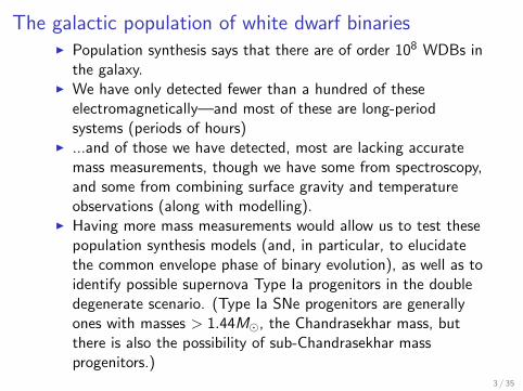
The galactic population of white dwarf binariesI Population synthesis says that there are of order 108 WDBs in
the galaxy.I We have only detected fewer than a hundred of these
electromagnetically—and most of these are long-periodsystems (periods of hours)
I ...and of those we have detected, most are lacking accuratemass measurements, though we have some from spectroscopy,and some from combining surface gravity and temperatureobservations (along with modelling).
I Having more mass measurements would allow us to test thesepopulation synthesis models (and, in particular, to elucidatethe common envelope phase of binary evolution), as well as toidentify possible supernova Type Ia progenitors in the doubledegenerate scenario. (Type Ia SNe progenitors are generallyones with masses > 1.44M�, the Chandrasekhar mass, butthere is also the possibility of sub-Chandrasekhar massprogenitors.)
3 / 35
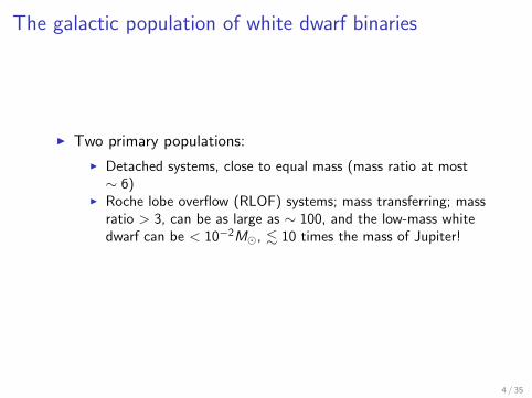
The galactic population of white dwarf binaries
I Two primary populations:
I Detached systems, close to equal mass (mass ratio at most∼ 6)
I Roche lobe overflow (RLOF) systems; mass transferring; massratio > 3, can be as large as ∼ 100, and the low-mass whitedwarf can be < 10−2M�, . 10 times the mass of Jupiter!
4 / 35

A RLOF system
HM Cnc, the shortest-period AM CVn system known (321 s), as envisioned by
Rob Haynes (LSU).
5 / 35
mHz gravitational wave detectors: Prospects andterminology
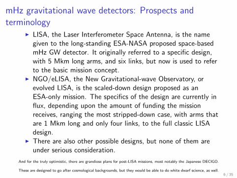
I LISA, the Laser Interferometer Space Antenna, is the namegiven to the long-standing ESA-NASA proposed space-basedmHz GW detector. It originally referred to a specific design,with 5 Mkm long arms, and six links, but now is used to referto the basic mission concept.
I NGO/eLISA, the New Gravitational-wave Observatory, orevolved LISA, is the scaled-down design proposed as anESA-only mission. The specifics of the design are currently influx, depending upon the amount of funding the missionreceives, ranging the most stripped-down case, with arms thatare 1 Mkm long and only four links, to the full classic LISAdesign.
I There are also other possible designs, but none of them areunder serious consideration.
And for the truly optimistic, there are grandiose plans for post-LISA missions, most notably the Japanese DECIGO.
These are designed to go after cosmological backgrounds, but they would be able to do white dwarf science, as well.6 / 35

mHz gravitational wave detectors: Prospects andterminology (cont.)
LISA classic5 Mkm armssix links
NGO/eLISA (stripped-down)1 Mkm arms“mother–daughter”configuration, four links
7 / 35
GW detectors and white dwarf binaries
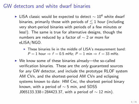
I LISA classic would be expected to detect ∼ 104 white dwarfbinaries, primarily those with periods of . 1 hour (includingvery short-period binaries with periods of a few minutes orless!). The same is true for alternative designs, though thenumbers are reduced by a factor of ∼ 2 or more foreLISA/NGO.
I These binaries lie in the middle of LISA’s measurement band:P = 1 hour ⇒ f = 0.5 mHz; P = 1 min ⇒ f = 33 mHz.
I We know some of these binaries already—the so-calledverification binaries. These are the only guaranteed sourcesfor any GW detector, and include the prototype RLOF systemAM CVn, and the shortest-period AM CVn and eclipsingsystems known to date: HM Cnc, the shortest period binaryknown, with a period of ∼ 5 min, and SDSSJ065133.338+284423.37, with a period of ∼ 12 min).
8 / 35
Low-frequency gravitational wave detectors and whitedwarf binaries (cont.)2 T. B. Littenberg, S. L. Larson, G. Nelemans, N. J. Cornish
Config. !!
Sa!
Sx Links
(m) (m/s2/!
Hz) (m/!
Hz)
1 1 " 109 4.5 " 10!15 11 " 10!12 4
2 2 " 109 3.0 " 10!15 10 " 10!12 63 5 " 109 3.0 " 10!15 18 " 10!12 6
Table 1. Gravitational wave detector configurations used in thisstudy. Configuration 1 corresponds to eLISA. Configuration 5 isthe classic LISA design. All simulations were for two year missionlifetimes.
dreds of sources that can be observed both electromagneti-cally and gravitationally.
The information encoded about the UCBs in each ofthe two spectrums is highly complementary, enabling testsof general relativity, full measurement of the physical pa-rameters enabling constraints on binary synthesis channels,and new methods of probing the close interaction dynamicsof the compact stars (Cutler et al 2003; Stroeer et al 2005).
2 DETECTORS
For a gravitational wave observatory, the limiting sensitivityas a function of frequency is dominated at low frequencies byacceleration noise Sa, while the “floor”, where the detector ismost sensitive, is dominated by position measurement noiseSx. Table 1 contains the parameters used for the detectorconfigurations in this study. These parameters can be usedto compute the noise power spectral density
Sn(f) = Sgal(f) + (4/3) sin2 u [(2 + cos u)Sx
+ 2(3 + 2 cos u + cos 2u)Sa/(2!f)4!, (1)
where u = 2!f"/c and Sgal is the contribution tothe instrument noise from the unresolved UCB fore-ground (Timpano et al 2006).
The configurations we will highlight correspond to theclassic LISA design (" = 5 Gm), as well as two shorter arm-length configurations (" = 2 Gm and " = 1 Gm) in orderto cover a variety of plausible mission configurations. The 1Gm configuration is similar to the eLISA mission being con-sidered by the European Space Agency (Amaro-Seoane et al2012). We use an observation time of two years for each con-figuration.
This suite of detectors provides a broad palette to il-lustrate the observational capabilities of these instrumentswith regards to the UCBs. A classic depiction of the per-formance for these interferometers is a plot of the averagesensitivity curve in strain spectral density versus frequency(Larson et al 2000), as shown in Fig. 1. The eLISA con-cept is the only one which uses a 4-link configuration. Thedoppler ranging between each spacecraft in the constella-tion is accomplished using two laser links. Thus the 4-linkdesign is a single-vertex interferometer, while the 6-link de-signs allow for three (coupled) interferometers. This di!er-ence accounts for an additional improvement in the 6-linksensitivity curves by a factor of !
"2 at frequencies where
the UCBs are found.
10-20
10-19
10-18
10-17
10-16
10-4 10-3 10-2
S h(f)
1/2 H
z-1/2
f (Hz)
Config 1 (eLISA)Config 2 Config 3 (LISA)
1000 loudest binariesKnown verification binaries
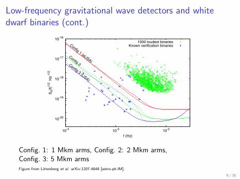
Figure 1. Sensitivity curve for each of the detector configura-tions in Table 1. The solid lines show the sensitivity set by themeasurment noise while the dashed curves include an estimateof the UCB confusion-limited foreground. Over-plotted are thebrightest UCBs in our simulated catalog (green crosses), and the
known verification binaries (blue stars)
3 DISCOVERING NEW VERIFICATIONBINARIES
The focus of this work is to study the population of de-tectable UCBs in the context of multi-messenger astronomy.We will focus on the sources detected via GWs which couldpotentially be identified electromagnetically. There is a sep-arate class of UCBs, the “verification binaries,” which areknown low-frequency GW sources with AM CVn servingas the archetype. There are ! 30 known verification bi-naries, ! 5 # 10 of which could be identified by the GWdetectors considered here, with sources still being discov-ered (Nelemans 2011; Roelofs et al 2007; Brown et al 2011).This study does not include the known verification binariesin the galaxy catalogs. Furthermore, many of the AM CVnsystems would not be localized well enough by the GW mea-surement alone to warrant simple electromagnetic follow-upobservations.
3.1 Binary selection
The UCB population model is essentially identical to thatfound in Nelemans et al (2004), so the positions and ages ofthe systems are based on the Boissier & Prantzos (1999)Galactic model. We use the white dwarf cooling tracksbased on Hansen (1999) as shown in the Appendix ofNelemans et al (2004). We convert the luminosities to V-band magnitudes using zero-temperature white dwarf radiiand simple bolometric corrections based on the e!ectivetemperature. This should su"ce for this initial estimate ofthe potentially detectable population, but can be improvedusing detailed WD cooling models in the future. We deter-mine the absorption as in Nelemans et al (2004) based onthe Sandage (1972) model, but correcting for the fact thatthe dust is more concentrated than the stars, so we use 120pcas scale height for the absorption.
To construct the magnitude limited catalog, we beginwith the entire binary population in the synthesized galaxy.The limiting apparent magnitude of a telescope is a function
c# 2012 RAS, MNRAS 000, 1–6
Config. 1: 1 Mkm arms, Config. 2: 2 Mkm arms,Config. 3: 5 Mkm armsFigure from Littenberg et al. arXiv:1207.4848 [astro-ph.IM].
9 / 35
GW detectors and white dwarf binaries (cont.)
I At low frequencies, the binaries are so numerous that theyform a confusion foreground for LISA. However, this does notconcern us, since we are primarily concerned with strongsources.
I These strong binaries will be detected by LISA at high SNRs(some > 1000 for LISA classic), since one can integrate thesignal for the entire mission (at least one year, possibly severalyears in optimistic scenarios). (This requires knowing thebinary’s phase evolution, but that can be obtained fromelectromagnetic observations to the needed accuracy for thebinaries we consider—getting it from LISA alone may be morecomplicated.)
10 / 35
Information in the GW signal
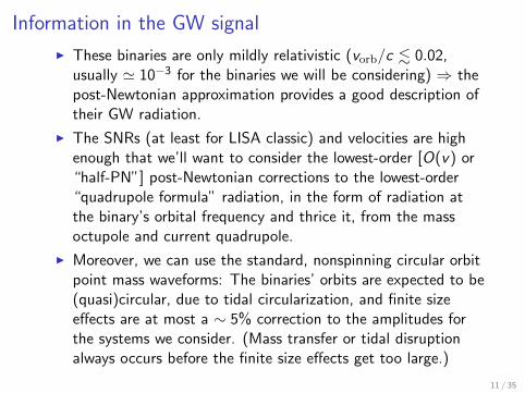
I These binaries are only mildly relativistic (vorb/c . 0.02,usually ' 10−3 for the binaries we will be considering) ⇒ thepost-Newtonian approximation provides a good description oftheir GW radiation.
I The SNRs (at least for LISA classic) and velocities are highenough that we’ll want to consider the lowest-order [O(v) or“half-PN”] post-Newtonian corrections to the lowest-order“quadrupole formula” radiation, in the form of radiation atthe binary’s orbital frequency and thrice it, from the massoctupole and current quadrupole.
I Moreover, we can use the standard, nonspinning circular orbitpoint mass waveforms: The binaries’ orbits are expected to be(quasi)circular, due to tidal circularization, and finite sizeeffects are at most a ∼ 5% correction to the amplitudes forthe systems we consider. (Mass transfer or tidal disruptionalways occurs before the finite size effects get too large.)
11 / 35

Information in the GW signal (cont.)The point mass, circular orbit waveform is
h+ = −()M5/3ω2/3
r(1 + cos2 θ) cos 2Φ +
(µδm)ω
r[() cos Φ + () cos 3Φ]
h× = −()M5/3ω2/3
rcos θ cos 2Φ +
(µδm)ω
r[() cos Φ + () cos 3Φ],
with relative errors of O(v2orb/c
2).
I M := (m1m2)3/5/(m1 + m2)1/5 is the binary’s so-called chirpmass (the name comes from its appearance in a point massbinary’s frequency evolution)
I µδm = m1m2(m1 −m2)/(m1 + m2)
I ω is the binary’s orbital angular frequency
I r is the binary’s distance
I θ is the binary’s inclination angle
I Φ is the binary’s phase
12 / 35
Information in the GW signal (cont.)
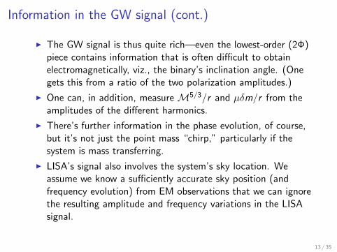
I The GW signal is thus quite rich—even the lowest-order (2Φ)piece contains information that is often difficult to obtainelectromagnetically, viz., the binary’s inclination angle. (Onegets this from a ratio of the two polarization amplitudes.)
I One can, in addition, measure M5/3/r and µδm/r from theamplitudes of the different harmonics.
I There’s further information in the phase evolution, of course,but it’s not just the point mass “chirp,” particularly if thesystem is mass transferring.
I LISA’s signal also involves the system’s sky location. Weassume we know a sufficiently accurate sky position (andfrequency evolution) from EM observations that we can ignorethe resulting amplitude and frequency variations in the LISAsignal.
13 / 35
What can electromagnetic observations add?
I First, knowing the sky position and frequency evolutionimproves LISA’s accuracy.
I If we know a distance and another combination of the masses,we can obtain the binary’s individual masses. (One only needs one
additional measurement if one is able to measure the higher harmonics.)
14 / 35
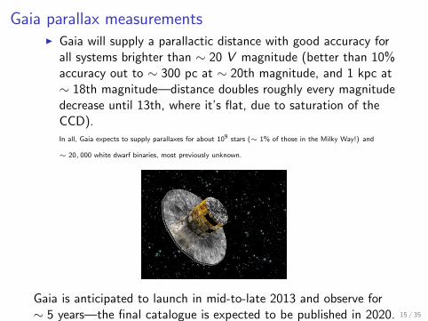
Gaia parallax measurementsI Gaia will supply a parallactic distance with good accuracy for
all systems brighter than ∼ 20 V magnitude (better than 10%accuracy out to ∼ 300 pc at ∼ 20th magnitude, and 1 kpc at∼ 18th magnitude—distance doubles roughly every magnitudedecrease until 13th, where it’s flat, due to saturation of theCCD).In all, Gaia expects to supply parallaxes for about 109 stars (∼ 1% of those in the Milky Way!) and
∼ 20, 000 white dwarf binaries, most previously unknown.
Gaia is anticipated to launch in mid-to-late 2013 and observe for∼ 5 years—the final catalogue is expected to be published in 2020. 15 / 35
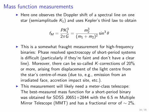
Mass function measurementsI Here one observes the Doppler shift of a spectral line on one
star (semiamplitude K1) and uses Kepler’s third law to obtain
fM =PK 3
1
2πG=
m32
(m1 + m2)2sin3 θ
I This is a somewhat fraught measurement for high-frequencybinaries: Phase resolved spectroscopy of short-period systemsis difficult (particularly if they’re faint and don’t have a clearline). Moreover, there can be so-called K -corrections of 20%or more, arising from displacement of the light centre fromthe star’s centre-of-mass (due to, e.g., emission from anirradiated face, accretion impact site, etc.).
I This measurement will likely need a meter-class telescope:The best-measured mass function for a short-period binarywas obtained for SDSS J0651+2844 with the 6.5 m MultipleMirror Telescope (MMT) and has a fractional error of ∼ 2%.
16 / 35
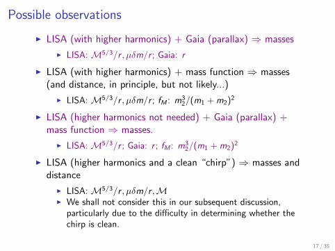
Possible observations
I LISA (with higher harmonics) + Gaia (parallax) ⇒ masses
I LISA: M5/3/r , µδm/r ; Gaia: r
I LISA (with higher harmonics) + mass function ⇒ masses(and distance, in principle, but not likely...)
I LISA: M5/3/r , µδm/r ; fM : m32/(m1 + m2)2
I LISA (higher harmonics not needed) + Gaia (parallax) +mass function ⇒ masses.
I LISA: M5/3/r ; Gaia: r ; fM : m32/(m1 + m2)2
I LISA (higher harmonics and a clean “chirp”) ⇒ masses anddistance
I LISA: M5/3/r , µδm/r ,MI We shall not consider this in our subsequent discussion,
particularly due to the difficulty in determining whether thechirp is clean.
17 / 35

General scheme of measurementI LISA first detects a binary, measuring its period and obtaining
a rough sky localization.I One then searches electromagnetically for a binary at that
period in LISA’s error box. Could be 10s of square degrees or larger in many cases,
though high-SNR binaries will be localized to square arcminutes, at least with LISA classic
I One expects a variation in luminosity at the system’s orbitalperiod for many of these systems, due to eclipses, hot spots,accretion disks, etc. Ellipsoidal variability has already been observed in several DWD
systems.
I Once one has a precise sky location, one can consult the Gaiacatalogue for a parallax (if the system is brighter than ∼ 20thmagnitude) and/or attempt to make a mass functionmeasurement.
I One also folds the information about the sky location andphasing back in to the LISA analysis, to improve parameterestimation.
(If the binary is already known electromagnetically, then things areeasy, but this is only applicable to a few presently known binaries.)
18 / 35
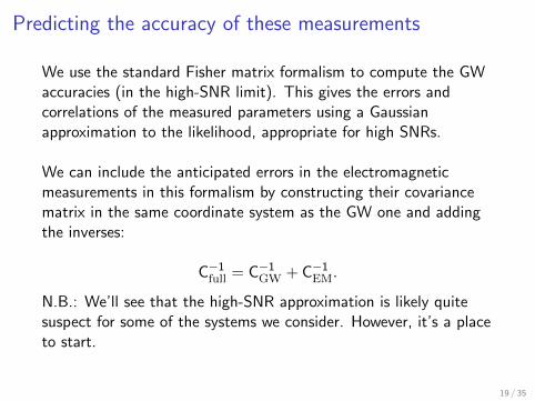
Predicting the accuracy of these measurements
We use the standard Fisher matrix formalism to compute the GWaccuracies (in the high-SNR limit). This gives the errors andcorrelations of the measured parameters using a Gaussianapproximation to the likelihood, appropriate for high SNRs.
We can include the anticipated errors in the electromagneticmeasurements in this formalism by constructing their covariancematrix in the same coordinate system as the GW one and addingthe inverses:
C−1full = C−1
GW + C−1EM.
N.B.: We’ll see that the high-SNR approximation is likely quitesuspect for some of the systems we consider. However, it’s a placeto start.
19 / 35
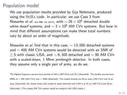
Population modelWe use population results provided by Gijs Nelemans, producedusing the SeBa code. In particular, we use Case 3 fromNissanke et al. ApJ 758, 131 (2012), with ∼ 26× 106 detached doublewhite dwarf systems, and ∼ 3× 10⁶ AM CVn systems. But bear inmind that different assumptions can make these total numbersvary by about an order of magnitude.
Nissanke et al. find that in this case, ∼ 13, 000 detached systemsand ∼ 400 AM CVn systems would be detected with an SNR of≥ 5 with classic LISA, and ∼ 6, 300 detached and ∼ 90 AM CVnwith a scaled-down, 1 Mkm armlength detector. In both cases,they assume only a single pair of arms, as do we.
The highest-frequency sources have periods of 185 s (AM CVn) and 76 s (detached). The loudest sources have
SNRs of ∼ 500 (AM CVn) and ∼ 2500 (detached). The closest binaries are 65 pc away (AM CVn) and 14 pc
away (detached); the closest binary that would be easily detected with LISA is at 97 pc (AM CVn) and 28 pc
(detached). (The closest AM CVn system would be marginal with LISA classic.)
20 / 35
Models for the accuracy of electromagnetic measurements
Since Gaia’s predicted accuracy is given in terms of the system’sapparent magnitude, we need to compute this, which we do usinga model for the system’s absolute magnitude (i.e., its intrinsicluminosity), and its distance, plus a model for the extinction(interstellar absorption) in the galaxy, for which we use the onefrom Bahcall and Soneira ApJS 44, 73 (1980).
We use the models of Nelemans et al. MNRAS 349, 181 (2004) for theluminosity of the accretion disk in the AM CVn systems and theirfits to white dwarf cooling curves for the detached systems, with afiducial cooling time of 108 years.
21 / 35

Results for LISA + Gaia
0 500 1000 1500 2000P (s)
0.1
0.2
0.3
0.4
0.5
Fra
cti
on
al
mass
err
or
m1, LISA classic
m2, LISA classic
m1, NGO 2 km
m2, NGO 2 km
(These are all detached systems.)
22 / 35
ES Cet with LISA + Gaia + mass function
0 0.1 0.2 0.3 0.4 0.5Fractional accuracy in the mass function measurement
0.05
0.1
0.15
0.2
0.25
0.3
0.35
0.4
Fra
ctio
nal
acc
ura
cy i
n t
he
mas
s m
easu
rem
ent
LISA classic, m1
LISA classic, m2
NGO 2 km, m1
NGO 2 km, m2
NGO 1 km, m1
NGO 1 km, m2
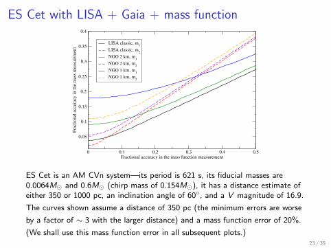
ES Cet is an AM CVn system—its period is 621 s, its fiducial masses are0.0064M� and 0.6M� (chirp mass of 0.154M�), it has a distance estimate ofeither 350 or 1000 pc, an inclination angle of 60◦, and a V magnitude of 16.9.
The curves shown assume a distance of 350 pc (the minimum errors are worse
by a factor of ∼ 3 with the larger distance) and a mass function error of 20%.
(We shall use this mass function error in all subsequent plots.)23 / 35
Results for LISA + Gaia + mass function
0 0.04 0.08 0.12 0.16 0.2 0.24 0.28 0.32 0.36 0.4σ
m1
/m1
0
25
50
75
100
125
150
Nu
mb
er o
f sy
stem
s
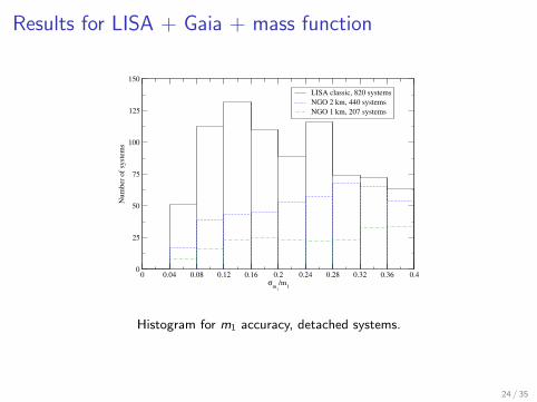
LISA classic, 820 systems
NGO 2 km, 440 systems
NGO 1 km, 207 systems
Histogram for m1 accuracy, detached systems.
24 / 35
Results for LISA + Gaia + mass function
0 0.04 0.08 0.12 0.16 0.2 0.24 0.28 0.32 0.36 0.4σ
m2
/m2
0
50
100
150
200
250
300
350
400
450
500
Nu
mb
er o
f sy
stem
s
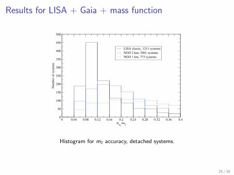
LISA classic, 1211 systems
NGO 2 km, 1061 systems
NGO 1 km, 773 systems
Histogram for m2 accuracy, detached systems.
25 / 35
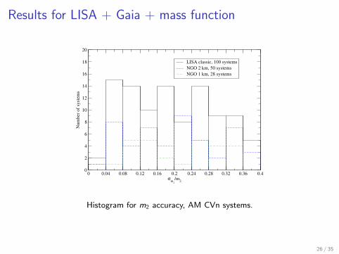
Results for LISA + Gaia + mass function
0 0.04 0.08 0.12 0.16 0.2 0.24 0.28 0.32 0.36 0.4σ
m2
/m2
0
2
4
6
8
10
12
14
16
18
20
Nu
mb
er o
f sy
stem
s
LISA classic, 100 systems
NGO 2 km, 50 systems
NGO 1 km, 28 systems
Histogram for m2 accuracy, AM CVn systems.
26 / 35
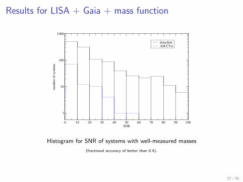
Results for LISA + Gaia + mass function
0 10 20 30 40 50 60 70 80 90 100SNR
1
10
100
1000
nu
mb
er o
f sy
stem
s
detachedAM CVn
Histogram for SNR of systems with well-measured masses
(fractional accuracy of better than 0.4).
27 / 35

Results for LISA + Gaia + mass function
0 0.5 1 1.5 2 2.5 3m (solar masses)
0
0.1
0.2
0.3
0.4
σm
/m
Fractional accuracy of total mass measurement versus total mass,
for LISA classic, detached systems, 987 total
28 / 35
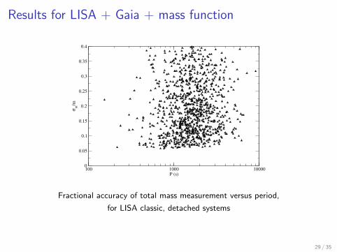
Results for LISA + Gaia + mass function
100 1000 10000P (s)
0
0.05
0.1
0.15
0.2
0.25
0.3
0.35
0.4
σm
/m
Fractional accuracy of total mass measurement versus period,
for LISA classic, detached systems
29 / 35
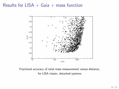
Results for LISA + Gaia + mass function
10 100 1000r (pc)
0
0.05
0.1
0.15
0.2
0.25
0.3
0.35
0.4
σm
/m
Fractional accuracy of total mass measurement versus distance,
for LISA classic, detached systems
30 / 35

Results for LISA + Gaia + mass function
We would be able to measure the total masses of 26 potentialType Ia supernova progenitors (all detached) with LISA classic withsufficient accuracy to say that they indeed have such high masseswith 95% confidence. With 2 km armlength eLISA/NGO, thenumber goes down to 12, and with 1 km arms, it goes down to 5.
(The highest-frequency potential Type Ia SNe progenitors in thepopulation model will coalesce in thousands of years. However,these systems are all many kpc away. The systems we would detectwith this measurement will be much lower frequency and closer by,and will not coalesce for hundreds of thousands of years—usuallymillions of years.)
31 / 35
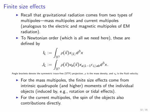
Finite size effects
I Recall that gravitational radiation comes from two types ofmultipoles—mass multipoles and current multipoles(analogous to the electric and magnetic multipoles of EMradiation).
I To Newtonian order (which is all we need here), these aredefined by
IL :=
∫R3
ρ(~x)x〈L〉d3x
JL :=
∫R3
ρ(~x)vb(~x)xa〈L−1εil 〉abd3x .
Angle brackets denote the symmetric trace-free (STF) projection, ρ is the mass density, and va is the fluid velocity.
I For the mass multipoles, the finite size effects come fromintrinsic quadrupole (and higher) moments of the individualobjects (induced by, e.g., rotation or tidal effects).
I For the current multipoles, the spin of the objects alsocontributions directly.
32 / 35
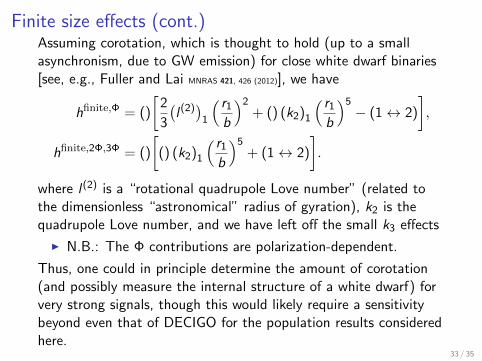
Finite size effects (cont.)Assuming corotation, which is thought to hold (up to a smallasynchronism, due to GW emission) for close white dwarf binaries[see, e.g., Fuller and Lai MNRAS 421, 426 (2012)], we have
hfinite,Φ = ()
[2
3
(l (2))
1
( r1b
)2+ () (k2)1
( r1b
)5− (1↔ 2)
],
hfinite,2Φ,3Φ = ()
[() (k2)1
( r1b
)5+ (1↔ 2)
].
where l (2) is a “rotational quadrupole Love number” (related tothe dimensionless “astronomical” radius of gyration), k2 is thequadrupole Love number, and we have left off the small k3 effects
I N.B.: The Φ contributions are polarization-dependent.
Thus, one could in principle determine the amount of corotation(and possibly measure the internal structure of a white dwarf) forvery strong signals, though this would likely require a sensitivitybeyond even that of DECIGO for the population results consideredhere.
33 / 35
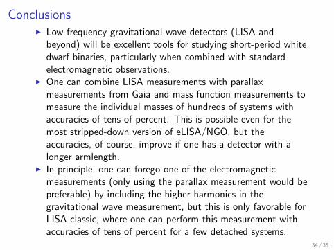
ConclusionsI Low-frequency gravitational wave detectors (LISA and
beyond) will be excellent tools for studying short-period whitedwarf binaries, particularly when combined with standardelectromagnetic observations.
I One can combine LISA measurements with parallaxmeasurements from Gaia and mass function measurements tomeasure the individual masses of hundreds of systems withaccuracies of tens of percent. This is possible even for themost stripped-down version of eLISA/NGO, but theaccuracies, of course, improve if one has a detector with alonger armlength.
I In principle, one can forego one of the electromagneticmeasurements (only using the parallax measurement would bepreferable) by including the higher harmonics in thegravitational wave measurement, but this is only favorable forLISA classic, where one can perform this measurement withaccuracies of tens of percent for a few detached systems.
34 / 35
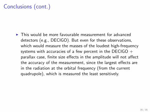
Conclusions (cont.)
I This would be more favourable measurement for advanceddetectors (e.g., DECIGO). But even for these observations,which would measure the masses of the loudest high-frequencysystems with accuracies of a few percent in the DECIGO +parallax case, finite size effects in the amplitude will not affectthe accuracy of the measurement, since the largest effects arein the radiation at the orbital frequency (from the currentquadrupole), which is measured the least sensitively.
35 / 35