Approved by:

Gary Bishop, Advisor

Mary Whitton, Reader

Anselmo Lastra, Reader

James Coggins

Frederick P. Brooks, Jr.

Measuring the Perceived Visual Realism of Images

by

Pablo Mauricio Rademacher

A dissertation submitted to the faculty of the University of North Carolina at Chapel

Hill in partial fulfillment of the requirements for the degree of Doctor of Philosophy in the

Department of Computer Science.

Chapel Hill

2002

ii

2002

Pablo Mauricio Rademacher

ALL RIGHTS RESERVED

iii

ABSTRACT

Pablo Mauricio Rademacher: Measuring the Perceived Visual Realism of Images

(Under the direction of Dr. Gary Bishop)

One of the main goals of computer graphics research is to develop techniques for

creating images that look real – i.e., indistinguishable from photographs. Most existing work

on this problem has focused on image synthesis methods, such as the simulation of the

physics of light transport and the reprojection of photographic samples. However, the

existing research has been conducted without a clear understanding of how it is that people

determine whether an image looks real or not real. There has never been an objectively

tested, operational definition of realism for images, in terms of the visual factors that

comprise them. If the perceptual cues behind the assessment of realism were understood,

then rendering algorithms could be developed to directly target these cues.

This work introduces an experimental method for measuring the perceived visual

realism of images, and presents the results of a series of controlled human participant

experiments. These experiments investigate the following visual factors: shadow softness,

surface smoothness, number of objects, mix of object shapes, and number of light sources.

The experiments yield qualitative and quantitative results, confirm some common assertions

about realism, and contradict others. They demonstrate that participants untrained in

computer graphics converge upon a common interpretation of the term real, with regard to

images. The experimental method can be performed using either photographs or computer-

generated images, which enables the future investigation of a wide range of visual factors.

iv

To Lisa

v

ACKNOWLEDGEMENTS

I would like to thank:

Gary Bishop for years of guidance and friendship.

Jed Lengyel, Ed Cutrell, and Turner Whitted, for enabling, supporting, and enthusiastically participating in this research.

Mary Whitton for raising the quality of this dissertation.

My dissertation committee: Gary Bishop, Frederick Brooks, James Coggins, Anselmo Lastra, and Mary Whitton, for encouraging the pursuit of difficult questions.

Microsoft Research for providing the funding, facilities, and assistance that made this work possible.

The UNC Department of Computer Science for providing a rich environment in which ideas thrive.

My professors at West Virginia University, especially William “Chip” Klostermeyer, Cun-Quan “C.Q.” Zhang, John Goldwasser, Frances VanScoy, and John Randolph, for sharing their love of mathematics and computer science.

The National Science Foundation for financial support.

The Research Triangle Institute for providing the SUDAAN statistical analysis software.

My parents for always encouraging me in every endeavor.

My wife, Lisa, for her patience, support, and love.

vi

TABLE OF CONTENTS

LIST OF TABLES................................................................................................................ x

LIST OF FIGURES ............................................................................................................ xii

1. Introduction.....................................................................................................................1

1.1 Motivation ............................................................................................................1

1.2 Experimental method for measuring the perceived visual realism of images ..........3

1.3 Thesis statement....................................................................................................4

1.4 Summary of experimental results ..........................................................................5

1.5 Overview of dissertation........................................................................................7

2. Background.....................................................................................................................9

2.1 Computer graphics research on realistic image synthesis .......................................9

2.1.1 Image-based rendering ................................................................................9

2.1.2 Physically-based rendering........................................................................ 10

2.2 Artistic methods for visual realism ...................................................................... 11

2.3 Research on the human visual system and visual perception................................ 11

2.4 Applications of human vision research to computer graphics............................... 13

2.4.1 Rendering methods for simulating direct vision......................................... 13

2.4.2 Image quality measures based on visual perception ................................... 14

2.4.3 Perceptual experiments using computer graphics....................................... 15

2.5 Summary............................................................................................................. 17

3. Method For Investigating the Perceived Realism of Images........................................... 18

3.1 Selection of participants ...................................................................................... 19

vii

3.2 Experimental instructions and task ...................................................................... 20

3.2.1 Experimental instructions.......................................................................... 20

3.2.2 No explicit definition of “real” or “not real”.............................................. 22

3.2.3 Operational definition of realism............................................................... 23

3.2.4 Experimental task...................................................................................... 23

3.2.5 Wording of experimental task ................................................................... 25

3.3 Active vs. passive assessments of realism............................................................ 27

3.4 Photographs and computer-generated images are not mixed ................................ 28

3.5 Object arrangement ............................................................................................. 28

3.6 Analysis method.................................................................................................. 31

3.7 Logistic regression model.................................................................................... 33

4. Overview of Experiments .............................................................................................. 35

4.1 Factors under investigation.................................................................................. 35

4.2 Image creation..................................................................................................... 38

4.3 Image presentation .............................................................................................. 40

4.4 Participant selection and compensation ............................................................... 41

4.5 Determination of outliers..................................................................................... 41

5. Photograph-Based Experiments on Shadow Softness And Surface Smoothness ................................................................................................................... 42

5.1 Introduction......................................................................................................... 42

5.2 Shadow softness.................................................................................................. 43

5.2.1 Experimental setup.................................................................................... 43

5.2.2 Results: ℜ vs. shadow softness.................................................................. 46

5.3 Surface smoothness ............................................................................................. 49

5.3.1 Experimental setup.................................................................................... 49

5.3.2 Results: ℜ vs. surface smoothness............................................................. 50

viii

5.4 Interaction effects between shadow softness and surface smoothness .................. 51

6. Photograph-Based Experiments on Number of Objects, Mix of Object Shapes, and Number of Light Sources ........................................................................... 53

6.1 Number of objects and mix of object shapes........................................................ 53

6.1.1 Experimental setup.................................................................................... 53

6.1.2 Results: ℜ vs. number of objects ............................................................... 55

6.1.3 Results: ℜ vs. mix of object shapes ........................................................... 57

6.1.4 Interaction between number of objects and mix of object shapes ............... 58

6.2 Number of light sources ...................................................................................... 59

6.2.1 Experimental setup.................................................................................... 59

6.2.2 Creation of images .................................................................................... 60

6.2.3 Results: ℜ vs. number of light sources ...................................................... 62

6.3 Number of participants and power....................................................................... 64

7. Experiments Using Computer-Generated Images........................................................... 68

7.1 Setup................................................................................................................... 69

7.2 Results: ℜ vs. shadow softness (computer-graphics-based experiment) ............... 72

7.3 Results: ℜ vs. surface smoothness (computer-graphics-based experiment) .......... 75

7.4 Comparison of photograph-based and computer-graphics-based shadow softness and surface smoothness experiments...................................................... 76

8. Discussion..................................................................................................................... 78

8.1 Experimental results ............................................................................................ 78

8.1.1 Discussion: shadow softness and surface smoothness ................................ 78

8.1.2 Discussion: number of objects, mix of object shapes, and number of light sources.......................................................................................... 80

8.2 Reliability, sensitivity, and validity ..................................................................... 81

8.3 Results support thesis statement .......................................................................... 83

8.4 Summary............................................................................................................. 84

ix

9. Future Work.................................................................................................................. 85

9.1 Other visual factors ............................................................................................. 85

9.1.1 Color......................................................................................................... 85

9.1.2 Global illumination ................................................................................... 86

9.1.3 Geometric complexity ............................................................................... 86

9.1.4 Surface texture .......................................................................................... 86

9.1.5 Motion ...................................................................................................... 87

9.2 Method of adjustment.......................................................................................... 87

9.3 Do viewers look for realistic or for unrealistic features in images? ...................... 87

Appendix: Data ................................................................................................................... 89

A.1 Raw data: photograph-based experiment on shadow softness and surface smoothness.......................................................................................................... 89

A.2 Scene-collapsed data: photograph-based experiment on shadow softness and surface smoothness ....................................................................................... 94

A.3 Raw data: photograph-based experiment on number of objects and mix of object shapes ....................................................................................................... 95

A.4 Scene-collapsed data: photograph-based experiment on number of objects and mix of object shapes ..................................................................................... 97

A.5 Raw data: photograph-based experiment on number of lights .............................. 98

A.6 Scene-collapsed data: photograph-based experiment on number of lights .......... 100

A.7 Raw data: computer-graphics-based experiment on shadow softness ................. 101

A.8 Scene-collapsed data: computer-graphics-based experiment on shadow softness ............................................................................................................. 103

A.9 Raw data: computer-graphics-based experiment on surface smoothness ............ 104

A.10 Scene-collapsed data: computer-graphics-based experiment on surface smoothness........................................................................................................ 105

References ........................................................................................................................ 106

x

LIST OF TABLES

Table 1. Summary of experimental results. ........................................................................6

Table 2. Example on how to calculate ℜℜℜℜ for surface smoothness experiment (numbers are fictitious). ℜℜℜℜ is calculated in the same manner for data from a single participant and for data from all participants. ℜℜℜℜ is entirely independent of the origin of image (photographic or computer-generated). ........25

Table 3. Logistic regression model for photograph-based experiment on shadow softness and surface smoothness. .......................................................................42

Table 4. Test statistics for brightness and contrast............................................................45

Table 5. Test statistics for photograph-based shadow softness experiment. ......................47

Table 6. Test statistics for pair-wise comparisons in photograph-based shadow softness experiment............................................................................................48

Table 7. Test statistics for comparison of top two levels in photograph-based shadow softness experiment...............................................................................49

Table 8. Test statistics for photograph-based surface smoothness experiment. .................51

Table 9. Test statistics for interaction between surface smoothness and shadow softness in photograph-based experiment. ..........................................................52

Table 10. Logistic regression model for experiment on number of objects and mix of object shapes......................................................................................................53

Table 11. Test statistics for photograph-based experiment on number of objects................56

Table 12. Test statistics for pair-wise comparisons in photograph-based experiment on number of objects..........................................................................................57

Table 13. Test statistics for photograph-based experiment on mix of object shapes............58

Table 14. Test statistics for interaction between number of objects and mix of object shapes. ...............................................................................................................59

Table 15. Logistic regression model for experiment on number of light sources. ...............59

Table 16. Test statistics for photograph-based experiment on number of light sources...............................................................................................................64

xi

Table 17. Test statistics for photograph-based shadow softness and surface smoothness experiments, using data from nine participants that also performed experiments on number of objects and mix of object shapes..............66

Table 18. Test statistics for photograph-based shadow softness and surface smoothness experiments, using data from six participants that also performed experiment on number of light sources..............................................67

Table 19. Logistic regression model for CG-based experiment on shadow softness. ..........70

Table 20. Logistic regression model for CG-based experiment on surface smoothness. .......................................................................................................70

Table 21. Test statistics for computer-graphics-based experiment on shadow softness. .............................................................................................................74

Table 22. Test statistics for pair-wise comparisons in computer-graphics-based experiment on shadow softness. .........................................................................74

Table 23. Test statistics for comparison of last four levels in computer-graphics-based shadow softness experiment. ....................................................................75

Table 24. Test statistics for computer-graphics-based experiment on surface smoothness. .......................................................................................................76

Table 25. Test statistics for photograph-based and computer-graphics-based experiments on shadow softness and surface smoothness. ..................................77

xii

LIST OF FIGURES

Figure 1. Is this image real or not real? How did you decide?.............................................2

Figure 2. Natural images tend to have a power distribution of 1/ƒ2. ..................................13

Figure 3. Written instructions given to participants. ..........................................................21

Figure 4. Sample screenshot from experiment on shadow softness. ...................................26

Figure 5. Sample screenshot from experiment on number of objects. ................................27

Figure 6. Example of multiple spatial arrangements (scenes), taken from photograph-based shadow softness experiment (Chapter 5). Each row has a different arrangement of objects. For each arrangement, all five levels of shadow softness are represented (across columns)..............................................30

Figure 7. Sample images from photograph-based shadow softness experiment. Shadow softness varies across columns, from hardest (left) to softest (right). Spatial arrangement of objects varies between rows. .............................44

Figure 8. Detail of images from photograph-based shadow softness experiment. Average penumbra angles for the five shadow levels were .39°, 1.5°, 2.5°, 5.2°, and 10.2°. ..................................................................................................44

Figure 9. ℜℜℜℜ vs. shadow softness for photographic experiment. Bar height indicates the proportion of “real” responses across all participants and images, for each shadow level. Error bars indicate ±1 standard deviation from the mean. The increase in ℜℜℜℜ was statistically significant. Note: the x-axis is not evenly scaled. ..............................................................................................46

Figure 10. Detail of two images from photograph-based surface smoothness experiment. The smooth, spray-painted cubes (left) rated much lower in realism than the rough, brush-painted cubes (right). ...........................................50

Figure 11. ℜℜℜℜ vs. surface smoothness for photographic experiment. Images with rough textures rated much higher (statistically significant) than images with smooth textures. .........................................................................................50

Figure 12. Sample images from experiment on number of objects and mix of object shapes. The number of objects increases across columns, and the mix of object shapes (cubes-only versus cubes and rounded objects) varies between rows.....................................................................................................55

xiii

Figure 13. Results of photograph-based experiment on number of objects. There was no statistically significant effect. Note: the x-axis is not evenly scaled. .............55

Figure 14. Results of photograph-based experiments on mix of object shapes. There was no statistically significant effect. .................................................................58

Figure 15. Sample images from experiment on number of light sources. From left to right, images have one, two, and four light sources. Top row has hard shadows; bottom row has soft shadows. There was no statistically significant effect with respect to number of light sources. ..................................62

Figure 16. Results of photograph-based experiment on number of light sources. There was no statistically significant effect ........................................................62

Figure 17. Graphs of shadow softness and surface smoothness responses, using data from nine participants that also performed experiments on number of objects and mix of object shapes. .......................................................................66

Figure 18. Graphs of shadow softness and surface smoothness responses, using data from six participants that also performed experiment on number of light sources...............................................................................................................66

Figure 19. Sample images from computer-graphics-based shadow softness experiment. Shadow softness varies across columns, from hardest (left) to softest (right). Object arrangement varies between rows....................................71

Figure 20. Detail of images from CG-based shadow softness experiment. Average penumbra angles for the five shadow levels were 0°, 1.5°, 2.5°, 5.2°, and 10.3°. .................................................................................................................71

Figure 21. Detail of images from CG-based surface smoothness experiment. The bump maps for the computer-generated objects were acquired by photographing the faces of the cubes used in the photograph-based surface smoothness experiment. .....................................................................................72

Figure 22. Results of computer-graphics-based experiment on shadow softness. There was a statistically significant increase in ℜℜℜℜ. The greatest increase in reported realism occurred between the first and second levels. ...........................73

Figure 23. Results of computer-graphics-based experiment on surface smoothness. These closely match the results from the photograph-based experiment. The increase in ℜℜℜℜ was statistically significant. ...................................................76

1. INTRODUCTION

1.1 Motivation

Realistic rendering is one of the main areas of research in computer graphics (CG).

In many applications, the goal of realistic rendering is to create images that are perceived by

human observers as being real, and not synthetic. The objective is for computer-generated

images to evoke a similar sense of perceived visual realism as that evoked by direct

photographic captures of existing physical scenes. This is the aim, for example, of visual

effects for live-action films – viewers should believe that the computer-generated elements

are as real as the photographed elements. While the goal of perceived visual realism is

common, not much is known about why some images are perceived as real and others are

not. There is very little data in the literature of computer graphics, visual perception, art, or

photography to indicate what about an image tells observers that it is real.

The lack of data on what causes images to be perceived as real hinders research on

realistic rendering. For example, perceived visual realism is often equated with physical

accuracy. It is reasoned that accurate computational simulations of the physical processes of

light transport and photography will lead directly to realistic imagery. The fallacy of this

reasoning lies in the presumption that photographs are always regarded as realistic. If real-

world photographs, which are the product of real-world light transport, are not all perceived

as realistic, then simulating these physical processes does not suffice to guarantee realistic

imagery. Instead, it becomes necessary to focus on those specific visual cues that suggest

realism to observers.

Evidence of why certain images are perceived as real would also help prioritize

research on the different elements of an image (lighting quality, surface texture, geometric

2

structure and detail, etc). There is no data in the literature as to which visual factors

contribute most to realism, and which visual factors have no effect.

Figure 1. Is this image real or not real? How did you decide?

In this dissertation I measure the perceived visual realism of images, as reported by

human participants via an experimental task. I obtain data on how changes along different

visual factors affect perceived visual realism. The modifier perceived is necessary because

the experimental method measures participants’ regard of images as being either real or not

real, rather than measuring an inherent property in the images themselves.

The experimental data are used to answer broad questions about perceived visual

realism (e.g., whether all photographs are perceived as equally realistic), as well as narrower

questions on specific visual factors (e.g., whether perceived visual realism increases with

shadow softness or with the number of objects in a scene). The long-term goal of this line of

research is to discover exactly the manner in which different factors affect perceived visual

realism, so that new rendering algorithms can directly target the necessary visual cues.

3

1.2 Experimental method for measuring the perceived visual realism of images

In the experimental method used in this dissertation, study participants are presented

with a set of images on a CRT monitor. Participants rate each image as being either “real” or

“not real.” The images are controlled and vary only along specific visual dimensions1

(shadow softness, surface smoothness, number of objects, mix of object shapes, and number

of light sources). Participants are not told what the differences are between the images.

They are told only that each image may be either a photograph or a computer-generated

image (this establishes the context in which the term real operates). Participants are not

given an explicit definition of the term real, and they are free to apply any criteria they

choose in order to evaluate the images.

This work is based on the notion that people have an internal concept of realism that

they cannot directly verbalize, but which can be indirectly measured via an experimental

task. The experimental method thus yields an operational definition of the term “real.” An

operational definition [Brid60] of an abstract concept is a definition in terms of a specific

measurement procedure and an accompanying set of measurements. In this dissertation, a

visually realistic image is defined operationally as one that is rated as “real” by human

observers.

The goal of this research is not to measure people’s ability to correctly distinguish

between photographs and computer-generated images, but rather to measure how changes

along specific visual dimensions affect perceived visual realism. For this reason, the images

within each experiment must be identical except along those dimensions that are being

directly manipulated. This implies that within a given experiment the images must all be

photographic or they must all be computer-generated. The two should not be mixed, as this

would likely introduce confounding factors.

1 The terms visual factors and visual dimensions will be used interchangeably throughout this dissertation.

4

1.3 Thesis statement

The goal of this dissertation is to measure the effect different visual factors have on

perceived visual realism. The work investigates the following three-part thesis:

There exist visual factors in images which have measurable, consistent effects on perceived visual realism, as reported by human observers.

Not all visual factors have the same effect on perceived visual realism.

Certain visual factors have similar effects on perceived visual realism in both photographs and computer-generated images.

The thesis statement consists of three parts, which will be proven by the results of a

set of human participant experiments. These experiments investigated the following five

visual factors: shadow softness, surface smoothness, number of objects, mix of object shapes,

and number of light sources.

The first part of the thesis states that manipulating images along certain visual

dimensions yields differences in perceived visual realism that are consistent among different

observers (i.e., statistically significant). Of the five visual dimensions investigated,

statistically significant effects were observed for shadow softness and for surface smoothness

(Chapter 5).

The second part of the thesis states that not all visual factors have the same effect on

perceived visual realism. Whereas shadow softness and surface smoothness were found to

have statistically significant effects on reported realism, significant effects were not observed

for number of objects, mix of object shapes, or number of light sources (Chapter 6).

The third part of the thesis states that results are consistent for certain visual

dimensions, between photograph-based experiments and experiments based on computer-

generated images. In Chapter 7, CG-based experiments on shadow softness and surface

smoothness are compared to the photograph-based shadow and surface experiments from

Chapter 5.

5

1.4 Summary of experimental results

For each experiment, participants were asked to rate each image in a randomly

ordered series as either “real” or “not real.” These responses were converted to binary scores

by assigning the value zero for “not real,” and the value one for “real.” Summing the binary

scores over all participants at each level of a visual factor, and then dividing by the number

of scores at that level, gives a mean score. A mean score of zero for a given factor level

indicates that none of the images at that level were rated as “real,” while a mean score of one

indicates that all images at that level were rated as “real.” If participants expressed no

preference towards “real” or “not real” for a given factor level, or if they chose their

responses at random, then the expected mean score would equal 0.5. Furthermore, if they

rated the same number of images at each level as “real,” then the mean scores would be equal

across all levels, indicating that the visual factor had no effect. However, if the visual factor

did have a consistent effect on participants’ responses, then the mean scores will either

increase or decrease as the visual factor is varied. This is what the analysis tests: did

variations within each visual dimension affect participants’ responses? In practice, the mean

scores will almost never be exactly the same across the factor levels. Statistical analysis is

therefore employed to determine whether existing differences are likely due to an actual

effect or due only to chance.

The raw binary data were analyzed by repeated measures logistic regression analysis

(an analogue to repeated measures linear regression, but suitable for analysis of binary data).

The null hypothesis was that manipulations along each visual dimension has no effect on

participants’ responses. This was tested using the logistic regression’s p-value, which

indicates the statistical probability that differences in the mean scores across the factor levels

were due to chance (i.e., that a visual factor had no measurable effect). An α value of .05

was selected in advance of performing the experiments, with p < α indicating statistical

significance (i.e., that differences in the data were likely due to actual effects).

The results of the experiments are summarized below. For each experiment, the table

gives the number of participants, the number of levels tested for the visual factor, the mean

response score at each level (over all trials and all participants), the standard deviation of this

score, the overall model Chi-square value, and the p-value test for statistical significance.

6

The experiments were conducted over four two-day sessions, spaced approximately

three weeks apart. Each participant completed all of his or her experiments in a single two-

hour sitting at one of these sessions. The experiments on number of objects, mix of object

shapes, and number of light sources were added in the later sessions, hence the reduced

number of participants for these visual factors. The row entitled “Experimental Session”

shows the sessions in which each experiment was conducted.

Shadows softness

(photo)

Surface

smoothness

(photo)

Number of

objects

(photo)

Mix of

object

shapes

(photo)

Number of

light sources

(photo)

Shadow softness

(CG)

Surface

smoothness

(CG)

Number of

participants 18 18 9 9 6 7 7

Experimental

session I, II, III I, II, III II, III II, III III IV IV

Number of

trials per

participant

60 60 40 40 36 30 12

Number of

levels 5 2 4 2 3 5 2

Mean score at

each level .47, .52, .55, .62, .59 .39, .71 .73, .61, .64, .53 .60, .64 .46, .39, .36 .38, .72, .67, .77, .77 .27, .77

Std. dev. at

each level .12, .11, .11, .10, .11 .10, .12 .16, .20, .18, .15 .12, .17 .16, .16, .20 .22, .13, .20, .05, .17 .10, .13

Model chi-

square (d.f.=1) 4.32 12.85 3.12 0.56 0.50 5.46 18.75

p-value .0377 .0003 .0772 .4550 .4790 .0197 <.0001

Statistically

significant at

αααα=.05?

Yes Yes No No No Yes Yes

Table 1. Summary of experimental results.

The data in the table above proves the three parts of the thesis statement. First, two of

the visual factors, shadow softness and surface smoothness, yielded effects that were

statistically significant – i.e., measurable and consistent across different observers. Second,

7

not all the visual factors had the same effect on perceived visual realism – shadow softness

and surface smoothness were statistically significant, but number of objects, mix of object

shapes, and number of lights were not statistically significant. Third, results were consistent

between photograph-based experiments and experiments based on computer-generated

images, for the two visual factors that were tested in both forms.

1.5 Overview of dissertation

Chapter 2 – Background

This chapter reviews relevant previous research in computer graphics

and visual perception. Despite the fact that there is much crossover

work between these two fields, the central question of this

dissertation (“What visual factors cause an image to be perceived as

real?”) has not been directly studied in the existing literature.

Chapter 3 – Experimental method for investigating perceived visual realism

in images

This chapter discusses the many issues of experimental design that

must be considered for the proposed experimental method.

Chapter 4 – Overview of experiments

This chapter summarizes the visual factors investigated in this

dissertation, and discusses how the factors were selected.

Chapter 5 – Photograph-based experiments on shadow softness and surface

smoothness

This chapter presents photograph-based experiments exploring the

effects of shadow softness and surface smoothness on perceived

visual realism. Both visual factors had a statistically significant

effect on the reported realism.

8

Chapter 6 – Photograph-based experiments on number of objects, mix of

object shapes, and number of light sources

This chapter presents photograph-based experiments that measure

whether perceived visual realism varies with number of objects, mix

of object shapes, or number of light sources. These visual factors did

not have a statistically significant effect on reported realism.

Chapter 7 – Experiments using computer-generated images

This chapter presents CG-based experiments on shadow softness and

surface smoothness. The findings are shown to be consistent with

the photograph-based experiments on shadow softness and surface

smoothness from Chapter 5.

Chapter 8 – Discussion

This chapter discusses the results of the experiments from Chapters

5, 6, and 7.

Chapter 9 – Future work

The experiments I present in this dissertation only begin to explore

the complex problem of perceived visual realism. This chapter

describes some possible directions for future work.

2. BACKGROUND

There is little previous work that investigates how different visual factors affect

perceived visual realism. Existing research on image synthesis has not directly asked why

images look real, even though the answer to this question is essential for realistic rendering.

Research on human vision has not directly investigated the question either.

This chapter presents previous work from the following areas: realistic image

synthesis, art, human vision and visual perception, and applications of human vision research

to computer graphics. The relevance of existing work to perceived visual realism – the topic

of this dissertation – is discussed for each of these areas.

2.1 Computer graphics research on realistic image synthesis

This section discusses two leading approaches to realistic rendering in computer

graphics: image-based rendering and physically-based rendering.

2.1.1 Image-based rendering

Image-based rendering [Leng98] is a technique in which images of a three-

dimensional scene are generated for novel viewpoints, by manipulating and reprojecting pre-

acquired images (or, more generally, samples) of the scene. This can be a synthetic scene (a

set of renderings is computed as a preprocess, and reprojected at run-time), or a real-world,

physical scene (photographs are taken, and reprojected at run-time).

Forms of image-based rendering include lumigraph/light field methods

[Gort96][Levo96], image warping [McMi95][Shad98][McAl99], and photogrammetry

[Faug93][Debe96][Pull97]. Each of these techniques has been shown to be capable of

generating images that resemble photographs from novel viewpoints. However, image-based

10

rendering sheds little light on the nature of perceived visual realism. If the original images

are photographs, then the resulting images will look like photographs – the realism of the

final image is simply carried over from the original input images. Image-based rendering

research does not answer the question of what it is about the original images that makes them

look real or not to begin with.

2.1.2 Physically-based rendering

Another method for synthesizing realistic images is to simulate the physical process

of light transport. This approach typically centers on global illumination and surface

reflectance. Global illumination describes the propagation of light throughout a three-

dimensional environment, and surface reflectance describes the distribution of light reflected

from a surface [Cohe93][Glas95]. The success of a global illumination rendering method is

usually gauged by its predictive ability – how similar the images it produces are to what a

real-world image (e.g., a photograph) of the same scene would be. Surface reflectance

models are often expected to be predictive as well, and are compared for accuracy against

real-world photometric measurements of sample surfaces. Error metrics for physically-based

rendering methods have been extensively studied [Lisc94][Lafo96][Patt97], and primarily

consist of numerical analyses of the various approximations in the simulation models.

A problem with physically-based approaches to rendering is that it has not been

proven that physical accuracy is necessary or sufficient for perceived visual realism. That is,

there is no existing evidence to indicate that all realistic images are physically accurate, or

that all physically accurate images are realistic. If the two are not equivalent, then it may be

that physical accuracy is not enough to guarantee realism, or that accuracy is not even

required for realism. If not all photographs are perceived as real, then merely simulating the

physical process of photography will not guarantee realistic images. In this case, it would be

worthwhile to instead seek out those specific visual cues that indicate to an observer that an

image is real or not real.

11

2.2 Artistic methods for visual realism

The pursuit of visual realism in synthetic images is not a new endeavor. It can be

traced back to the Renaissance, when concepts such as perspective projection were

discovered [Jans91]. Up until the 19th century, much of the focus in painting was on realistic

lighting, texture, and form. In the 1970's, the Photorealism school of painting emerged

(exemplified by artists such as Chuck Close and Richard Estes) with the goal of creating

paintings that look like photographs [Meis80][Meis93]. Unfortunately, the methods used by

the Photorealist painters have never been expressed in formal terms, and they remain a purely

artistic skill.

More recently, visual effects studios for feature films have achieved high levels of

realism using computer graphics. Their images are usually generated without using

physically-based rendering algorithms, due to the long rendering times and loss of artistic

control associated with physically-based methods [Kahr96][Barz97][Vaz00]. Instead of

employing accurate physical simulations to achieve realistic imagery, visual effects studios

rely on the skills of their artists, who possess an understanding of how an image must look in

order to be perceived as real. This understanding, however, remains entirely in the artistic

domain, and has not been documented in formal terms.

It should be noted that while visual effects studios do not often employ physically-

based rendering algorithms, it is possible that the artists are manually approximating

physically-accurate solutions in their images. The task of determining the important features

of such approximations remains an open problem.

2.3 Research on the human visual system and visual perception

While there is much existing research on the human visual system and visual

perception (see [Bruc96] and [Gord97] for overviews), the main question of this dissertation

has never been directly addressed by these fields, and the issue of why photographs and

computer graphics are perceived as real or synthetic has not been a focus of study. In this

section we discuss research in these fields that nonetheless is relevant to this dissertation.

12

An area that has received much attention in human vision research is the role of edges

in the visual field. These have been found to be very important to overall visual perception.

[Bruc96] discusses the neurological basis for the importance of edges (retinal cells form

receptive fields1 which respond to edges) and [Marr80] provides a high-level computational

explanation of how edges are utilized in visual perception. Because of their importance to

overall perception, it is possible that edges play a role in determining perceived visual

realism of images as well. This is an open research question.

Another area that has been studied extensively is the perception of reflectance versus

lightness. When viewing a surface, or an image of a surface, there is an inherent ambiguity

as to how much of the surface's observed brightness is due to its reflectivity, and how much

is due to the intensity of the light. Visual perception research has explored how the visual

system resolves this ambiguity [Gilc94][Adel96][Sinh93]. The perception of reflectance

versus lightness is relevant to perceived realism in the context of lighting mismatches. For

example, in digital compositing [Brin99], a single image is comprised of many individual

image layers, which are merged together. If the layers are not consistent in their lighting or

reflectance, then the resulting image will look unrealistic. No existing work has applied the

findings of research on the perception of reflectance and lightness to the problem of

perceived realism in digital compositing.

Another area that relates to perceived visual realism is the study of statistics of natural

images. It has been discovered that images of natural environments (forests, lakes, rivers,

clouds, etc.) tend to exhibit a power distribution proportional to 1/ƒ2 [Scha96], where ƒ is a

given spatial frequency. That is, in a Fourier decomposition of a typical natural image, low-

frequency coefficients will have greater amplitude than high-frequency coefficients, with a

1/ƒ falloff (power is defined as amplitude-squared). It has also been shown that certain

neural cells along the visual pathway are tuned to this statistical distribution [Parr00]. This

suggests that one possible requirement for a natural image to be perceived as real may be

1 A receptive field is a collection of cells in the visual pathway that responds maximally to a specific visual

input pattern, such as edges or spots [Bruc96].

13

adherence to a 1/ƒ2 power distribution. The relationship between image statistics and

perceived visual realism has not been explored in the existing literature.

Figure 2. Natural images tend to have a power distribution of 1/ƒ2.

2.4 Applications of human vision research to computer graphics

Findings from research on human vision have been applied to computer graphics in

several ways. One is to simulate the physiological properties of the visual system, in order to

develop rendering systems whose images approximate direct vision better. Another

application is to develop perceptual metrics to measure the perceived difference between

pairs of images. Other research efforts have investigated issues in computer graphics using

experimental methods adapted from the study of visual perception.

2.4.1 Rendering methods for simulating direct vision

Findings from traditional research on visual perception have been applied to the

creation of synthetic images that approximate direct vision. There are many physiological

and perceptual responses that cannot be elicited by images displayed on computer monitors,

due to limitations in modern displays’ dynamic range, resolution, and field of view. To

14

compensate for display limitations, the physiological and perceptual responses can be

simulated within the images themselves. For example, the visual system's adaptation to

brightness was modeled in a CG rendering algorithm by Ferwerda [Ferw96]. Images created

by this algorithm are blurry and have unsaturated colors when the image in intended to

represent low-light conditions. This simulates the visual system's decreased spatial and

chromatic sensitivity in low light. Another example of using findings from visual perception

for realistic rendering is found in [Spen95], which simulates glare induced by bright light

sources.

These methods attempt to create images that are “realistic” in the sense that they

simulate what the human visual system encounters when directly viewing physical scenes.

However, this dissertation is not concerned with direct vision. In this dissertation it is given

that the visual stimulus in question is a two-dimensional image (not direct vision) and the

issue is whether the image is regarded by observers as being a direct capture of a physical

scene, or a synthetic rendering of a virtual one.

2.4.2 Image quality measures based on visual perception

One of the goals of the research in this dissertation is to take first steps towards the

development of a metric for perceived visual realism in images. No such metric currently

exists. In this section we review existing work on perception-based image-difference

metrics, which provide insight on how to construct image metrics using findings from

research on human visual perception.

Non-perceptual image difference metrics, such as Root Mean Square Error, do not

accurately predict the difference between two images that would be noticed by a human

observer [Rush95]. Non-perceptual metrics do not take into consideration the human visual

system’s non-linear and space-varying sensitivity to contrast, lightness, spatial frequencies,

etc. [Bruc96]. To account for these, Daly [Daly93] developed the Visible Differences

Predictor (VDP), which incorporates perceptual properties of the human visual system in

order to predict the perceived difference between a pair of images. For example, the human

visual system’s response to sinusoidal gratings at different frequencies and amplitudes is well

understood. One of the tasks performed by the VDP is to apply these known response curves

15

to a frequency-based decomposition of a target image, in order to assess an observer’s ability

to discern features within that image. The output of the VDP is a Difference Map: a meta-

image that indicates the magnitude of perceived difference at each corresponding pixel in a

pair of input images. A competing model to the VDP is the Sarnoff Visual Discrimination

Model (VDM) [Lubi95], which places more emphasis on physiology than psychophysics.

Perception-based metrics such as the VDP and VDM have been used to optimize

image rendering algorithms by steering computational effort towards those regions with the

highest noticeable error (i.e., towards perceptually-important regions). A rendering

algorithm can then halt when the overall perceptual difference between successive rendering

steps is below some threshold. There are numerous examples of CG rendering algorithms

that incorporate the VDP, the VDM, or derivatives of these models

[Gibs97][Gadd97][Boli98] [Mysz99][Rama99]. A survey is given by [Prik99].

These existing works on perception-based metrics may serve as templates for future

work on perceived visual realism. One long-term goal that follows from this dissertation is

the development of a Perceived Visual Realism Map, which would attempt to predict the

magnitude of perceived visual realism at each region of an input image. This map could be

based in part on the findings of this dissertation. That is, if realism response curves have

been experimentally obtained for different visual factors, then by measuring these factors in a

target image, one may predict the realism rating that the image would be given by observers.

This could be incorporated into a rendering algorithm as well, in a manner similar to the

VDP and the VDM, by guiding computational rendering effort towards those image regions

that have low predicted realism.

2.4.3 Perceptual experiments using computer graphics

There have been many perceptual experiments conducted within the field of computer

graphics. Here we review the experiments that are relevant to visual realism.

The fidelity of one of the early radiosity systems was evaluated with a perceptual

experiment [Meye86]. Participants in the experiment viewed a real physical scene (the

“Cornell Box”) and a CG rendering of the same scene. The physical scene was captured with

a camera and displayed on a computer monitor, and the CG scene was directly displayed on a

16

second computer monitor. Participants were asked which of the two images was the real

scene. The goal of the experiment was to establish their perceptual similarity, by seeing

whether observers could correctly differentiate between the two. Participants chose correctly

in fifty-five percent of the trials (data was statistically equivalent to guessing), thereby

demonstrating that the rendering algorithm could create synthetic images that were

perceptually similar to real images of the scene. In contrast, the experimental method of this

dissertation does not directly compare computer generated images to reference photographs

in order to establish their similarity, but instead focuses on how changes along specific visual

dimensions – in both photographs and CG images – affect perceived visual realism.

McNamara [McNa98][McNa00] studied the fidelity of images created by different

illumination algorithms, including ray tracing [Glas89], radiosity [Cohe93], and the

Radiance software package [Ward94]. A rig was constructed that allowed participants to see

either a real physical scene, a photograph of that scene, or one of several computer-generated

images of that scene. The scene was a box containing a few simple objects. The CG images

varied in their rendering method (e.g., radiosity versus ray tracing) and in their rendering

parameters (e.g., the number of indirect light ray bounces). The participants' task was to

estimate the grayscale value of different regions within each image and different regions

within the physical environment. The task was not the assessment of real versus not real. A

novel perceptual metric of rendering fidelity was constructed based on the similarity between

the perceived grayscale values of the real scene (viewed directly) and the reported grayscale

values of the images. This metric can predict, given a set of parameters for a given rendering

algorithm, how similar a synthetic image created by that algorithm would be to direct

viewing. The metric does not, however, predict whether an image would be assessed as

“real” by observers. The experiment does not ask participants to report on how realistic they

believe each image is, but only to judge the grayscale lightness values of different regions

within the images.

[Thom98] and [Madi99] report on the results of an experimental evaluation of the

effect of shadows and global illumination on the perception of surface contact. A set of

rendered images was presented to participants, in which the images differed only in whether

shadows and global illumination were present or not. The goal was to experimentally

determine whether these visual factors had an effect on the perception of surface contact.

17

The results showed that shadows and global illumination significantly improved observers'

ability to detect contact between surfaces. The experimental method is similar to that of this

dissertation: a series of images is presented, one at a time, with a single question for

participants to answer for each image. The method of this dissertation, however, asks “is this

image real?” for each image, rather than “are these surfaces in contact?” Chapters 5 and 7 of

this dissertation present a photograph-based and CG-based experiment, respectively, which

investigate the effect of shadows on perceived visual realism.

2.5 Summary

There is much existing work on realistic image synthesis, but it has mainly focused

on how to create realistic images, not on why images as perceived as real. There are

artistically oriented methods for creating realistic imagery, but these have not been

verbalized in formal terms, and remain entirely in the artistic domain. There is much existing

research involving the human visual system and visual perception, but it has not focused on

perceived visual realism. There are visual perception experiments in computer graphics, but

they have focused on the fidelity of CG renderings, and have not directly investigated how

different visual factors affect an observer’s assessment of an image as being either real or not

real.

In this dissertation I address the problem of perceived visual realism with an

experimental method that asks participants to directly rate a series of images as either “real”

or “not real.” Participants are not asked to directly compare real and synthetic images to

each other. This dissertation is not interested in participants’ ability to correctly differentiate

between the two, but only in how changes along specific visual dimensions influence

observers’ assessments of visual realism.

3. METHOD FOR INVESTIGATING THE PERCEIVED REALISM OF IMAGES

This chapter describes a novel experimental method for studying the perceived visual

realism of images. The experimental method measures the effect that variations along

specific visual dimensions have on realism, as reported by participants. The method can be

used to study both photographs and computer-generated images. The method does not

measure participants’ ability to correctly differentiate between photographs and computer-

generated images – it instead measures the effect of different visual factors on participants’

assessments of images as being either real or not real.

Study participants are shown a randomized series of images, one at a time. They are

told in advance that each image will be either photographic or computer-generated. Their

task is to rate each as either “real” or “not real.” The images are controlled, and differ only

with regard to predetermined, manipulated visual factors. The participants’ pattern of

responses is later analyzed to determine which visual factors had a measurable effect on the

reported realism.

Although participants are instructed that the images are a mix of photographs and CG,

the images within a given experiment are in fact either all photographic or all computer-

generated. The two are not mixed, since the experimental design demands that the only

differences between images be along the manipulated visual factors.

The experimental method is based on standard principles from perceptual

experimentation, and the resulting data are analyzed with standard statistical techniques. The

experimental method has a repeated measures two-alternative forced-choice design [Levi94].

Each participant performs a number of trials (they view a number of images, one at a time)

with a two-choice selection task for each trial (rating each image as either “real” or “not

19

real”). This chapter describes the general experimental design. Subsequent chapters will

describe the specific experiments that were conducted for this research.

3.1 Selection of participants

This section discusses whether the experimental participants should be experts in a

visual field (such as computer graphics or photography), non-experts, or a mix of both. Each

approach has merits.

One of the possible advantages of employing experts in a visual field such as

computer graphics or photography is that experts might readily understand what is meant by

an image looking “real.” They might also already be familiar with the distinctions between

graphics and photographs. This a priori knowledge could presumably make the

experimental setup simpler, since experts might require fewer instructions at the beginning of

the experiment. Also, the resulting data could provide insights into the criteria used by

experts in their assessment of visual realism.

The problem with experts, however, is that they are already biased by their

experience. Professionals in computer graphics, for example, are already familiar with

common rendering artifacts (e.g., aliasing, sampling noise, and surface faceting) and may

specifically look for these artifacts. They know what can and what cannot be rendered with

current technology, and might interpret a particular image as photographic solely because

they know that it would be difficult to render with computer graphics. Conversely, they

might interpret an image as computer-generated simply because its content resembles

common CG images (e.g., it contains cubes, spheres, or teapots). They might respond to the

images in an experiment based on their expectations and knowledge of the field, rather than

on their true perceptions. Furthermore, it may be more useful to understand what non-

professionals think looks real, rather than professionals, since the ultimate audience for CG

images is usually the general public.

For the reasons above, the experiments in this dissertation employ only non-experts in

graphics or related visual fields. This does not affect the experimental design, but it does

affect the interpretation of the resulting data, which cannot necessarily be generalized to

experts. It is possible that experts have a different opinion of what looks real. There is no

20

guarantee, therefore, that the results in this dissertation will be consistent with results

obtained using experts.

The experimental method does not preclude the use of both experts and non-experts.

Performing experiments with both would permit a comparison of the two groups’ responses,

to determine if the given visual factors have the same effect on both experts and non-experts.

This would not change the experimental setup, but any interpretation of the resulting data

should address the expertise of the participants.

3.2 Experimental instructions and task

This section discusses the written instructions given to participants, as well as the

experimental task. It also discusses the operational definition of realism established by the

experimental task.

3.2.1 Experimental instructions

Care must be taken that the experimental instructions do not lead participants towards

any particular response. One common technique is to conceal the purpose of the experiment

until after the experiment is finished [Levi94, pg. 344]. Also, the instructions should explain

only what is essential for participants to know to be able to properly complete the

experimental task [Cool99]. These techniques prevent the participants from forming

expectations of how to respond.

Below are the written instructions given to participants. In the experiments

conducted for this dissertation, participants could ask questions, but only those questions that

related to the experimental procedure were answered (e.g., clarifications on how to change

one’s response if the wrong key is pressed).

21

Experimental Instructions

Today we are interested in gathering some

information about how people perceive images. In the

tasks that follow, you will see a number of images and

we will ask you to evaluate what you see. There is no

“right” or “wrong” answer to any response; we just want

to know what you think. As you look at these images,

try not to “think too much” about what you see. Go with

your first impression.

In this experiment we will show you a number of

images, one shown right after the other. Some of these

images are photographs of real objects, and others are

computer-generated. For each image, we want to know

whether you think it is real or not real. Sometimes it

may be a close call, but just do the best you can.

Figure 3. Written instructions given to participants.

The instructions convey the following:

• The experiment is investigating the perception of images.

Participants are told that this is a perceptual experiment, but they are

not told about the exact nature or purpose of the study.

• Not to “think too much” about the task.

Participants are instructed to go with their instinctive feeling on each

image, and not to worry about what the “correct” answer might be.

This is intended to reduce any anxiety, by telling participants that

they are not being scored on their performance.

22

• A series of images will be presented, some of which are photographs, and

others computer-generated.

This sets a context for the perceptual experiment, and states that each

image will fall under one of two categories. The instructions do not

tell how to distinguish the photographs from the computer-generated

images.

There is a small amount of deception involved, as all the images

within each experiment are of the same type, either photographic or

computer-generated. Photographs and computer-generated images

are never mixed in any single experiment. The reason for this is

discussed in Section 3.4.

• Their task is to label each image as either “real” or “not real.”

Participants are instructed to choose ones of the two options for each

image. There is no way for participants to indicate uncertainty over

any single image.

3.2.2 No explicit definition of “real” or “not real”

The experimental instructions do not explicitly define the terms “real” and “not

real,” nor do they elaborate on the visual differences between photographs and computer

graphics. The instructions present the two terms with no specific guidance on how decisions

should be made.

“Real” and “not real” are not necessarily common ways to think about images for

people who are not familiar with computer graphics, photography, or related visual fields.

One might expect that non-experts would have difficulty distinguishing between the two

types of images. However, if the instructions gave more detailed information, they could

bias participants’ responses.

Furthermore, the motivation for this research is the fact that it is not known what

makes an image look real. Therefore, an explicit definition of realism cannot be provided for

23

participants, because no such definition yet exists. We do not want to tell the participants

what causes images to look real – we want them to tell us.

3.2.3 Operational definition of realism

Instead of providing an explicit definition, the experiments let the participants define

realism through their responses. This is one of the basic principles of this experimental

method. The terms “real” and “not real” are presented, and participants interpret these words

– based on criteria of their choice – in response to the various visual factors in the images.

The experimental task and subsequent participant responses give an operational definition of

realism.

Operational definitions [Brid60] are standard components of psychological

experimentation. They are axiomatic, and define a concept in terms of the method used to

measure it and the subsequent measurements using that method.

An example of the use of operational definitions is the concept of intelligence – we

believe that there is such a thing, but what is it exactly? A non-operational definition of

intelligent might be “has high mental capacity” – but this says nothing of how to measure it

or recognize it in a person. In contrast, an operational definition might be “scores above 100

on an I.Q. test.” This provides a method of measurement and a range of measurements,

which together define the concept in question: any person that scores above 100 on an I.Q.

test would be considered intelligent under this definition. It is not an exhaustive or exclusive

definition, but it is one way to take an abstract concept and make it concrete.

The experimental method described in this dissertation operationalizes the abstract

concept of visual realism in a similar manner. A task is defined (participants rate a series of

images as either “real” or “not real”), and the pattern of responses relative to a given visual

factor is taken to be a measure of the perceived realism of the images across that factor.

3.2.4 Experimental task

A randomized series of images is presented to each participant, who rates each image

as either “real” or “not real.” The images vary according to some manipulated visual factors.

In this dissertation, the manipulated factors are shadow softness, surface smoothness, number

24

of objects, mix of object shapes, and number of lights. Each factor has a number of

predetermined levels that are tested. For example, in the experiment on surface smoothness

(Chapter 5) the factor can take one of two possible levels: rough and smooth – each image

shows either objects with rough surfaces or objects with smooth surfaces.

In this dissertation, the following three visual factors are measured along quantitative

scales: shadow softness (measured by penumbra angle), number of objects, and number of

lights. The remaining two visual factors – surface smoothness and mix of object shapes – are

not measured quantitatively. This is discussed further in Chapter 4.

The amount of data gathered at each factor level is increased by having participants

perform multiple trials for each level. For example, in the surface smoothness experiment,

multiple rough-surface images and multiple smooth-surface images are shown, rather than

only a single image for each of the two cases. By increasing the number of data points that

are measured, we increase the statistical power of the experiments. Section 3.5 discusses in

greater detail the creation of multiple images for each factor level.

The proportion of “real” responses for a particular level of a factor (i.e., the number

of images at that factor level that were rated as “real,” divided by the total number of images

at that factor level) is the realism response rating for that factor level. The realism response

rating is denoted in this dissertation by the symbol ℜℜℜℜ. Although participants give each

individual image only a binary score (“real” versus “not real”), the ℜℜℜℜ value for each factor

level is fractional. If we assign the numerical value of one to “real,” and zero to “not real,”

then ℜℜℜℜ is simply the mean of all numerical responses for a given factor level. ℜℜℜℜ can be

calculated for a single participant, across all participants, or for any combination of

participants. Also, ℜℜℜℜ is entirely independent of the origin of the image (photographic or

computer-generated) and it is calculated in the same manner for either case.

Here we present a fictional example to illustrate the computation of ℜℜℜℜ across all

participants. In the surface smoothness experiment (Chapter 5), each participant rates thirty

rough-surface images and thirty smooth-surface images. In this fictional example there are

ten participants who performed the experiment. Each participant rated 30 + 30 = 60 images,

for a total of 600 trials across all participants. The total numbers of “real” and “not real”

25

responses are given below, as well as the corresponding ℜℜℜℜ values for each of the two factor

levels (rough and smooth).

Number of trials

rated “real”

Number of trials

rated “not real”

Rough

surface 200 100

ℜℜℜℜrough = 200 / (200 + 100)

= .667

Smooth

surface 80 220

ℜℜℜℜsmooth = 80 / (80 + 220)

= .267

Table 2. Example on how to calculate ℜℜℜℜ for surface smoothness experiment (numbers are fictitious). ℜℜℜℜ is calculated in the same manner for data from a single

participant and for data from all participants. ℜℜℜℜ is entirely independent of the origin of image (photographic or computer-generated).

Instead of rating images only as “real” or “not real,” a different experimental task

would have been to rate each image along a multiple-point or continuous scale. This

complicates the experimental task by giving participants more than two choices for their

responses, and it requires a linearization step in the data analysis to account for non-

linearities in each participant’s interpretation of the linear scale. Furthermore, there is no

existing evidence in the literature to suggest that people are even able to differentiate

between more than two grades of visual realism (this question is discussed further in

Chapters 5 and 7).

3.2.5 Wording of experimental task

The experimental task is to rate images as “real” or “not real”, and not

“photographic” or “not photographic.” The intent is not to focus on specific qualities of

photography, but rather to investigate the general property of perceived visual realism. This

property is not exclusive to photographs – it may be possessed by a computer-generated

image, a painting, or any type of image with the potential of being perceived as a direct

26

capture of an existing physical scene. “Not real” is used in the experimental task instead of

alternatives such as “fake” or “synthetic” because “not real” is the direct negation of “real.”

Future work could study whether results would differ if the experimental question is changed

from “real” and “not real.” If the wording is changed, however, then the experimental

method will no longer be establishing an operational definition of the term real.

The experimental instructions do mention photographs and computer-generated

images, and provide a vague, implicit association between photographs/CG and real/not real.

This is intended to establish a context for the term real during the experiment, since real can

have several different interpretations. For example, a person might regard a photograph of a

physical sculpture of an alien creature as being “not real” because the creature is imaginary –

even though the image is of a real physical object. By stating that the images in the

experiment are either photographic or computer-generated, the instructions suggest that some

images are direct captures of physical objects, whereas others are synthetic renderings of a

virtual model. The instructions are not explicit in this association, and the words

“photograph” and “computer-generated image” are not mentioned elsewhere throughout the

experiment.

Figure 4. Sample screenshot from experiment on shadow softness.

27

Figure 5. Sample screenshot from experiment on number of objects.

3.3 Active vs. passive assessments of realism

A computer graphics professional might routinely look at images with the sole

purpose of deciding whether they look real. In contrast, a person untrained in graphics (such

as the participants in these experiments) may never have set out to determine if an image is

real or not real. Nonetheless, even when a person does not actively evaluate the realism of an

image, there are cases when they may passively make an assessment.

An active assessment of visual realism is when the observer is specifically looking at

an image in order to determine whether it looks real or not. The observer is aware that the

realism of the image is in question, and is looking for specific clues to determine its status.

A passive assessment of visual realism is one that is made when the observer is not

specifically intending to evaluate the realism of an image. The observer is not necessarily

aware that the realism of the image is in question, and is not specifically looking for evidence

for or against realism. An example of a passive assessment is someone watching a film when

a special effect suddenly stands out as being not real. The viewer may not have intended to

assess the realism of the image, but nonetheless some visual element became noticeably

28

unrealistic. One can also make a passive assessment in the opposite situation: some visual

element that is presumed to be not real may inadvertently stand out as looking real instead.

This experimental method only explores active assessments, since participants are told

in advance that they will be asked to judge each image as real or not real. The realism of any

given image is explicitly in question. The results of these experiments do not necessarily

generalize to the passive case, as active and passive evaluations of realism might behave

differently.

Future studies could determine the relationship (if any) between active and passive

assessments. A study of passive assessments would require an unobtrusive or nonreactive

form of measurement [Levi94, pg. 388], in which participants would have to be entirely

unaware of the target domain (visual realism).

3.4 Photographs and computer-generated images are not mixed

The goal of this experimental method is not to measure participants’ ability to

correctly identify photographs or computer-generated images. Instead, it is to measure how

participants’ responses change across the different levels of the manipulated visual factors.

Because of this, photographs and computer-generated images cannot be mixed in a single

experiment. If they were mixed, then there would be uncontrolled factors between the two

cases, unless the computer-generated images exactly matched the corresponding

photographs. Any uncontrolled factors would confound the analysis [Klei97]. For any

single experiment, therefore, the images must be either all photographs or all computer-

generated.

3.5 Object arrangement

The images in these experiments each show a small number of simple objects. There

are many possible ways in which these objects could be arranged (positioned and oriented).

The arrangement of objects affects the visibility of surfaces, the pattern of global

illumination, the number and size of shadows, and more. If only a single spatial arrangement

were used, then the results would be highly dependent on that particular arrangement and the

associated secondary factors. This would limit the generality of the results.

29

Furthermore, with only a single spatial arrangement, the steady repetition of similar-

looking images might cause the participants to lose interest. If the participants believed that

the same image was being repeatedly shown, then they might cease to evaluate each image

on its own merits, as an independent stimulus. They might instead rate all the images as a

group, believing them all to be the same image.

A solution is to use multiple spatial arrangements of objects instead of a single one.

That is, for each factor level, show more than one image, with different object arrangements.

This reduces the dependence of the results on any particular spatial arrangement, and it adds

visual variety to the image set. It also yields more data points at each factor level, which

increases the statistical power of the experiments. For these reasons, the experiments in this

dissertation employ multiple spatial arrangements of objects.

Another way to increase the number of data points would be by presenting every

image more than once. However, simple repetition would not reduce the results’ dependence

on a given spatial arrangement, nor would it increase the visual variety of the image set.

To illustrate the usage of multiple spatial arrangements, suppose that an experiment is

investigating a visual factor with five levels, and that three spatial arrangements of objects

(also referred to as scenes) are used. Let the five levels of the visual factor be labeled 1, 2, 3,

4, and 5, and let the three different spatial arrangements be labeled A, B, and C. Then the

experiment would consist of 5 × 3 = 15 images, labeled A1...A5, B1...B5, and C1...C5.

30

The spatial arrangement of objects is illustrated in the following figure, with images

taken from the experiment on shadow softness (Chapter 5):

Multiple spatial

arrangements

(scenes)

Figure 6. Example of multiple spatial arrangements (scenes), taken from photograph-based shadow softness experiment (Chapter 5). Each row has a

different arrangement of objects. For each arrangement, all five levels of shadow softness are represented (across columns).

The different spatial arrangements of objects are not required to have the same

perceived realism. It may be the case, for example, that a given spatial arrangement rates

significantly higher in realism, overall, than the other arrangements. For example, ℜℜℜℜA1…A5

might be higher than ℜℜℜℜB1…B5. That is, the reported realism of scene A might be higher than

that of scene B, across the five levels of the visual factor. However, this would not confound

the analysis. The data across different spatial arrangements are aggregated for each factor

level, and the statistical analysis measures response differences between factor levels, not

between spatial arrangements. The analysis for the visual factor in the example above would

compare the values {ℜℜℜℜA1..C1, ℜℜℜℜA2..C2, ℜℜℜℜA3..C3, ℜℜℜℜA4..C4, ℜℜℜℜA5..C5}, and not {ℜℜℜℜA1..A5, ℜℜℜℜB1..B5,

ℜℜℜℜC1..C5}. Since every spatial arrangement is represented for each level of the visual factor,

the arrangement of objects is orthogonal to the visual factor during the statistical analysis.

Besides the possibility of scenes not rating equally on overall realism, it may also be

the case that the spatial arrangement of objects interacts with the main visual factors under

investigation. For example, if one scene contains larger shadows than the other scenes, then

its perceived visual realism might be more strongly affected by shadow softness than the

31

other scenes. As discussed above, however, this would not affect the analysis of the main

visual factors under investigation (here, shadow softness), since the analysis of the main

effects considers the aggregate data across the scenes.

The spatial arrangements in this dissertation were not constructed in the same manner

as the main factors. For each of the five main visual factors under investigation, a scale was

determined along which to generate images. This scale was continuous for shadow softness,

discrete for number of objects and number of light sources, and binary for surface

smoothness and mix of object types. In contrast, the position and orientation of objects in

each scene was randomly determined, and there was no ordinal relationship between the

different scenes. Because of this, the scene variable cannot be placed on a meaningful metric

– it is a categorical, rather than numeric, variable [Klei97]. A test for statistical significance

of the scene variable could show that there exists a difference in realism between scenes, or

an interaction between scenes and main factors, but the test would not provide any

meaningful insight into the manner in which different arrangements of objects affect

perceived visual realism.

Because the spatial arrangement of objects was not designed to be analyzed

meaningfully like the main visual factors under investigation, and because one can validly

analyze the main visual factors without explicitly testing for differences between spatial

arrangements, I do not explicitly test whether spatial arrangement of objects has a statistically

significant main effect or interaction effect. This is left for future work, where spatial

arrangement of objects could be studied as a main visual factor, by constructing spatial

arrangements along some meaningful and quantifiable scale.

3.6 Analysis method

This experimental design is not intended to measure participants’ ability to correctly

distinguish between photographs and computer-generated images. It is therefore not

important within this research to think of the responses as hits, misses, false positives, false

negatives, etc., or to apply an analysis based on correctness of responses. This research is

instead designed to study how changes along various independent variables (the visual

factors) affect the participants’ realism ratings.

32

Linear regression and analysis of variance (ANOVA) [Levi94] are common analysis

methods for studying the change in a dependent variable as a function of a set of independent

variables. However, these techniques are valid only on normally distributed, continuous

data. In this dissertation, the response variable is binary.

An appropriate analysis method for the experimental design in this research is logistic

regression [Hosm00]. This is an adaptation of linear regression that is suitable for binary

data, and makes no assumptions about the distribution of the data. Logistic regression

computes the correlation between a manipulated factor and a binary response variable. For

each experiment in this research, a logistic regression analysis is used to test whether the

given factor (e.g., shadow softness or number of lights) has a significant effect on

participants’ responses of “real” versus “not real.” The null hypothesis in each test is that the

manipulated factor has no effect.

Logistic regression yields a p-value test statistic, whose function is identical to that of

p-values in linear regression. The p-value indicates the statistical probability that the data in

question would have been observed if there was no true effect. Low p-values are interpreted

as representing a high probability that there were measurable differences in the data – i.e.,

statistically significant effects [Chow96]. In the experiments conducted for this dissertation,

the level for asserting statistical significance was determined in advance to be p < .05. A p-

value of less than .05 indicates that there is at most a one in twenty probability that the

observed data would have resulted as such if the given factor had no true effect (i.e., if the

participants’ responses were random). In this research, we will also refer to p-values

between .05 and .10 as trends (also known as borderline effects), which indicate that there

may be an effect present, though the predetermined criteria for statistical significance was not

reached. Trends are often regarded as potential areas for future study.

Because each participant in these experiments performs many trials (and the

responses are therefore not independent), a repeated measures analysis [Wine91] is required.

This takes into account the correlation between responses by the same participant. The data

in this dissertation were analyzed using the Research Triangle Institute’s commercial

statistics package SUDAAN [Shah96][Biel97], which handles repeated measures logistic

regression designs. It outputs a number of statistics describing the data. The relevant

33

statistics presented in this report are the Chi-square1 value for each statistical test, and the

corresponding p-value test.

3.7 Logistic regression model

Logistic regression analysis in a single-factor experimental design is modeled as:

y = β0 + β1 x

where y is the dependent variable, x is the independent variable, and β0 and β1 are the

intercept and slope of the regression line, respectively. In logistic regression, the dependent

variable is defined as y = logit(p) = log(odds) = log(p / (1 − p)), where p is the probability of

an event [Hosm00]. In this research, p is the probability of an image being rated as real. The

independent variables are the various visual factors under investigation. The values β0 and

β1 are estimated by the regression analysis method. When the reported p-value is less than

.05, we consider the regression slope β1 to be statistically non-zero, and we say that a

measurable effect was detected. The regression model presented above is used to analyze the

single-factor experiments of Chapter 6 (on photograph-based number of light sources) and

Chapter 7 (on CG-based shadow softness and surface smoothness).

When two factors are studied simultaneously within a single factorial experimental

design, the model is:

y = β0 + β1 x1 + β2 x2 + β3 x1 x2

where y and β0 are as before, x1 and x2 are the two independent variables, β1 is the regression

slope of the first factor, β2 is the regression slope of the second factor, and β3 is the slope of

the interaction between the two factors. The values β1 and β2 relate to the main effects of the

experimental design – i.e., the effect of each factor separately, ignoring the other factor. The

value β3 relates to the interaction effect, which shows whether the effect of one factor was

different based on the value of the other factor. A statistically significant main effect for

either of the factors indicates that participants’ responses varied measurably with that factor.

1 The Chi-squared test statistic indicates the dissimilarity between the observed data and the data which would

be expected if the responses were random. A small Chi-squared value (close to zero) indicates that the observed values were likely random and not correlated with the independent variable.

34

When a statistically significant interaction effect is present, the effect of one factor depends

on the level of the other factor, and any discussion or interpretation of the factors must take

this into account. A two-factor experimental design does not presume that there will be an

interaction between the two factors.

The two-factor regression model with interaction, presented above, is used to analyze

the two-factor experiments of Chapter 5 (on photograph-based shadow softness and surface

smoothness) and Chapter 6 (on photograph-based number of objects and mix of object

shapes). Although the logistic regression analysis was performed for each case using the full

two-factor model presented above, the results are presented in separate sections for clarity

(first each main effect, then the interaction effect).

4. OVERVIEW OF EXPERIMENTS

The previous chapter discussed general design issues related to the experimental

method. This chapter discusses the specific experiments that were conducted for this

dissertation. It covers the selection of visual factors, the creation of images, the image-

presentation procedure, and the selection and compensation of participants.

4.1 Factors under investigation

The following criteria were used to select the visual factors to investigate in this

dissertation:

• Relevance to computer graphics – the visual factors should relate to current

issues in this field.

• Fundamental factors – the visual factors should be present in any image.

This gives the results wider applicability.

• Simplicity – the visual factors should be reasonably easy to manipulate, so

that images can be created without introducing extraneous, confounding

factors.

Based on these criteria, I selected five visual factors for investigation: shadow

softness, surface smoothness, number of objects, mix of object shapes, and number of light

sources. Photograph-based experiments were conducted for each of the five factors.

Computer-graphics-based experiments were conducted for shadow softness and surface

smoothness.

Because of the differing nature of the five visual factors, each was investigated with a

different number of levels. Two of the factors – surface smoothness and mix of object

shapes – did not possess a single numerical metric with which they could be measured.

36

There are many ways in which surfaces can vary in smoothness, and there are many ways to

classify the variety of object shapes in a scene. These two visual factors were therefore

reduced to binary variables: the surfaces in the image were either smooth or rough, and the

scene contained either a mixed or uniform selection of object shapes.

The remaining three visual factors possessed clear numerical scales on which they

could be measured. Shadow softness was measured by penumbra angle. Number of objects

and number of light sources were measured in the straightforward manner. Shadow softness

was investigated with five different levels, number of objects with four, and number of light

sources with three. The latter two experiments were tested with fewer levels due to practical

constraints in constructing the image set. As described in Chapter 6, constructing an

additional level for number of objects required doubling the number of physical objects in the

scene, and for number of light sources it required doubling the number of total photographs

to be taken.

Here is an overview of the visual factors and experiments:

• Shadow softness

Does perceived visual realism vary with the softness of shadows in the

image? This was studied with five shadow levels, ranging from very hard

shadows (from a spotlight) to very soft shadows (from a diffused light).

Shadow softness was tested in a photograph-based experiment (Chapter 5)

and in a CG-based experiment (Chapter 7). Separate pools of participants

performed each experiment, so there were no crossover effects between the

photograph-based and CG-based experiments.

• Surface smoothness

Does perceived visual realism vary with the smoothness of surfaces in the

image? Two levels were tested: “smooth” and “rough” surfaces. As with

shadow softness, this experiment was conducted in both photograph-based

form (Chapter 5) and CG-based form (Chapter 7).

37

The photographic smooth case showed spray-painted cubes, and the

photographic rough case showed brush-painted cubes. The computer-

graphics smooth and rough cases showed CG-rendered cubes, with texture

maps created from photographs of the real, physical cubes.

The photograph-based shadow softness and surface smoothness factors were

combined into a single experiment to allow for a test for interaction between

the two factors, in addition to the main effect test for each individual factor.

The total number of images for this photograph-based experiment was:

5 (shadow softness) × 2 (surface smoothness) ×

6 (object arrangements) = 60 images

The CG-based shadow softness and surface smoothness factors were studied

in separate experiments. I therefore only tested the main effect of each

individual factor, and not the interaction effect. The total number of images

in the CG-based shadow softness experiment was:

5 (shadow softness) × 6 (object arrangement) = 30 images

The total number of images in the CG-based surface smoothness experiment

was:

2 (surface smoothness) × 6 (object arrangements) = 12 images

Fewer images were created for the CG-based experiments than for the

photograph-based experiments due to time constraints in preparing and

rendering the CG images. The number of data points was nonetheless

sufficient to yield statistically significant results.

• Number of objects

Does perceived visual realism vary with the number of objects in the scene?

Four levels were tested, with images displaying two objects, four objects,

eight objects, and thirty objects. This experiment was conducted using only

photographs, and is described in detail in Chapter 6. Number of objects was

tested in conjunction with mix of object shapes, as described below.

38

• Mix of object shapes

Does perceived visual realism differ between images that have only one type

of object, and those that have multiple types of objects? This was tested

with two factor levels. In the first, all objects were cubes. In the second,

half the objects were cubes, and half the objects were curved shapes (spheres

and egg-shapes). This experiment was conducted using only photographs,

and is described in detail in Chapter 6.

The two factors, number of objects and mix of object shapes, were combined

into a single experiment to allow for a test for interaction, in addition to the

main effect test for each individual factor. The total number of images in

this experiment was:

4 (number of objects) × 2 (mix of object shapes) ×

5 (object arrangements) = 40 images

• Number of light sources

Does perceived visual realism vary with the number of light sources? There

were three levels in this experiment: images had either one, two, or four

lights. The softness of the shadows was also co-varied, with two levels

(hard and soft shadows). This experiment was conducted using only

photographs, and is described in detail in Chapter 6.

The total number of images in this experiment was:

3 (number of lights) × 2 (shadow softness) ×

6 (object arrangements) = 36 images

4.2 Image creation

All five visual factors were tested using photographs, and two were also tested using

computer-generated images. I acquired the photographs with an Olympus 3030Z digital

camera, at 800×600 pixel resolution. The green channel of each image was used to create a

39

grayscale image1. The camera was locked into place for the capture of all the images. The

scene objects were wooden cubes and spheres (5 centimeters tall), and wooden egg-shapes (7

centimeters tall). They were all painted white. In all the photographs, the objects were set

against a large white paper backdrop. All the photographs were taken at the same focal

distance, and the images were all downsampled internally by the digital camera (from its

internal resolution of 2048×1536) using the same downsampling algorithm. Because they

were constant across all the photographs, focal distance and downsampling were not

confounding factors. The digital camera’s location was held constant for all the photographs

within each experiment, and the shutter release was operated via remote control.

The images in the CG-based experiments were rendered using 3D Studio Max

[Disc02], with raytraced soft shadows. The CG objects were cubes, with bump maps

[Blin78] acquired by orthographically photographing the physical wooden blocks from the

photograph-based experiments. The intensity values of the maps were shifted to a common

mean, to ensure the various maps shared the same average intensity. The CG textures were

applied as bump maps instead of reflectance maps since the surface variations on the original

physical blocks were due to undulations in the paint layer (from the brush strokes), rather

than differences in the paint’s reflectance.

The CG images all had the same background, which was texture-mapped with a

photograph of the physical stage (the white backdrop). Indirect illumination (the reflection

of light from surfaces onto other surfaces) was not computed for any of the images. The

same anti-aliasing was used for all the CG images (a quadratic filtering kernel). Anti-

aliasing was therefore not a confounding factor. Since the CG images were all batch-

rendered from the same geometric and textural dataset, the CG version of the experiments

had precise experimental control.

All the images (photographs and CG) were generated with a single light source on the

right side (except for the experiment on number of lights, described in Chapter 6). When

each experiment was conducted, half the images were randomly selected at run-time to be

1 The green channel was chosen instead of the red channel, the blue channel, or a weighted blend of the three,

because the green channel carried the smallest amount of sensor noise with this digital camera. Nonetheless, any combination of channels could have been used, provided that the same combination was used for all the images (thereby ensuring experimental control).

40

shown flipped horizontally. This was randomized for each participant. Half the images

therefore appeared to have their light source on the right side, and half on the left side. This

was intended to increase the visual variety of the image set. Since the two image orientations

were evenly and randomly distributed, they cancel out and do not confound the analysis.

4.3 Image presentation

Image presentation and data collection were automated. Each image was displayed

on a CRT computer monitor against a gray background, with the captions “Not Real” and

“Real” below it in black. The participant chose a response by pressing either the ‘f’ key or

the ‘j’ key. When a key was pressed, the appropriate caption was highlighted (the text

changed color from black to white). The highlighting gave visual feedback of the response

that was selected. If the participant selected a different response than what she intended, she

could press the other key (‘f’ or ‘j’) to change the selection. The response for each image

was not finalized until the participant pressed the spacebar, which caused the entry to be

recorded and the experiment to proceed to the next image. The pace of the experiments was

therefore controlled by the participant.

The images were presented in groups of eight, where each group was shown in two

consecutive passes. In the first pass the images were only previewed, one at a time, and in

the second pass the participants rated the images, one at a time. The sequence of images in

the second pass was identical to that in the first. The preview pass showed the visual range

of upcoming images, to help participants calibrate their judgments. Since the total number of

images in each experiment did not always divide by eight, the last group of each experiment

could contain fewer than eight images.

At the start of each experiment, sixteen practice images (selected randomly from the

experimental set) were presented to familiarize the participant with the experiment. These

were presented in two groups of eight, as described above. The responses for these practice

trials were excluded from analysis. The images used for the practice trials were used again

for the main trials.

The order of image presentation was fully randomized for each participant. Each

participant conducted all of his or her image trials in one sitting. They were permitted to take

41

short breaks at any time. The total completion time for each participant ranged from 1 to 1½

hours.

The experiments were conducted in a room with controlled lighting, on PC

workstations with 21-inch CRT monitors. The monitors were not calibrated, but were

manually adjusted to match in brightness and contrast. Although these factors were not

strictly controlled, Chapter 5 presents an analysis that demonstrates that brightness and

contrast do not have a statistically significant effect on participants’ responses. The monitors

were set to a resolution of 1152×864, and each image had a resolution of 800×600.

Participants sat approximately two feet from the screen, giving a subtended viewing angle of

the images of approximately 30 degrees.

4.4 Participant selection and compensation

All participants were non-experts in computer graphics or related visual fields, aged

20 to 50, and had normal or corrected-to-normal vision. They all gave informed consent, and

were naïve to the study’s purpose. The experiments were performed at the Microsoft

Research Usability Labs in Redmond, Washington. Participants were chosen from a pool of

available candidates by a Participant Coordinator in the Microsoft Usability Group.

Participants were all non-Microsoft employees, and were each compensated with one piece

of Microsoft software.

4.5 Determination of outliers

I selected criteria, a priori, to determine when a participant’s data should be classified

as outlying. If a participant rated either more than 90% or less than 10% of the images as

“real” for a given visual factor, then all the data from that participant for the given visual

factor would be disregarded in the analysis. That is, a participant’s data would not be

included in the analysis for a given visual factor if he or she rated nearly all the images as

“real” or nearly all the images as “not real.”

There was only one participant who met this criteria. The data for this participant (as

well as the others, who were not classified as outliers) is included in the Appendix.

5. PHOTOGRAPH-BASED EXPERIMENTS ON SHADOW SOFTNESS AND SURFACE SMOOTHNESS

5.1 Introduction

This chapter presents experiments investigating the effect of shadow softness and

surface smoothness on perceived visual realism. All of the images shown to participants in

these experiments were photographs.

The two visual factors, shadow softness and surface smoothness, were tested within a

single experiment. Shadow softness was varied across five levels, from very hard shadows

(from a spotlight) to very soft shadows (from a diffused light source). Surface smoothness

was varied across two levels: smooth surfaces versus rough surfaces. The five levels of

shadow softness were crossed with the two levels of surface smoothness, and there were six

different spatial arrangements of objects. The experiment therefore contained 5 × 2 × 6 = 60

unique images.

Having the two factors in a single experiment allows us to test for interaction between

them. That is, to test whether the realism response behaves differently for one of the factors

depending on the level of the other factor. The logistic regression model1 for this experiment

is:

y = β0 + β1 ∗ SHADOW

+ β2 ∗ SURFACE

+ β3 ∗ SHADOW ∗ SURFACE

Table 3. Logistic regression model for photograph-based experiment on shadow softness and surface smoothness.

1 See Section 3.7 for a discussion of logistic regression models.

43

The statistics presented in this chapter result from the full model given above. For

clarity, the statistics for each main effect and for the interaction effect will be presented in

separate sections.

The order of image presentation was randomized for each participant at run-time. As

described in Section 4.2, half of the images (randomized per participant) were displayed

flipped horizontally. Each participant initially viewed and rated sixteen practice images,

selected randomly from the experimental set. The data from the practice trials is not included

in the analysis. The images used for the practice trials were used again for the main trials.

5.2 Shadow softness

5.2.1 Experimental setup

This experiment tested five levels of shadow softness, ranging from very hard to very

soft. The lowest level (hard shadows) was created with a spotlight (a 300W incandescent

light bulb inside a metallic housing), positioned 2.3 meters from the scene. The next two

levels were created with a 200W incandescent light bulb, progressively closer to the scene

(two and one meters, respectively). The closer distances made the shadows softer, while the

dimmer bulb intensity compensates for the increased illumination of the objects as the light

source moves closer. The last (softest) two levels were created with this same 200W light

source, diffused behind a sheet of white paper, at 1 meter and 20 centimeters, respectively.

The light positions were co-linear relative to the scene for all the images; the illumination

direction was therefore the same for all the photographs. Shadow softness increased

monotonically with each factor level.

The five shadow levels can be placed along a physically meaningful scale according

to the average penumbra angle of the images at each level. The penumbra angle was

measured from the bottom-most corner of the front-most object in each image. All the

objects in the photographs were cubes. The average penumbra angle at each shadow level

was .39°, 1.5°, 2.5°, 5.2°, and 10.3° (from hardest to softest). There were 12 images for each

of the five shadow softness levels.

44

Figure 7. Sample images from photograph-based shadow softness experiment. Shadow softness varies across columns, from hardest (left) to softest (right).

Spatial arrangement of objects varies between rows.

Figure 8. Detail of images from photograph-based shadow softness experiment. Average penumbra angles for the five shadow levels were

.39°, 1.5°, 2.5°, 5.2°, and 10.2°.

45

Because the different shadow levels were generated using lights at different distances

and with different intensities, the photographs varied in brightness and contrast. The

photographs were manually adjusted to correct any obvious exposure differences. The

remaining differences in brightness and contrast could potentially affect the results. In order

to verify that the results were not affected, I tested whether image brightness and image

contrast had a statistically significant effect on participants’ responses. The brightness and

contrast of each image was measured1, and used as independent variables in a repeated

measures logistic regression analysis of the data from the shadow softness and surface

smoothness experiments. Brightness and contrast were not found to have statistically

significant effects on participants’ responses. The following table gives the Chi-squared

value, the degrees of freedom2, and the p-value for brightness and contrast in this experiment:

ℜℜℜℜ vs. brightness and contrast:

CONTRAST: χ2=1.41, df=1, p=.2346 (not statistically significant) BRIGHTNESS: χ2=0.03, df=1, p=.8675 (not statistically significant)

Table 4. Test statistics for brightness and contrast.

The lack of precise experimental control when using photographs was one of the

motivations for verifying the results of this experiment using computer-generated images.

This is discussed in Chapter 7.

1 The mean and standard deviation of the pixel intensities in an image were taken as that image’s brightness and

contrast measures, respectively. The intensity of each pixel was measured as the unweighted average of the red, green, and blue values (each ranging from 0 to 255) of the pixel.

2 Since each test statistic refers to one independent variable, the degrees of freedom for each statistic is one.

46

5.2.2 Results: ℜℜℜℜ vs. shadow softness

ℜℜℜℜ

0.37 1.51 2.46 5.21 10.300.1

0.2

0.3

0.4

0.5

0.6

0.7

0.8

0.9

Penumbra Angle

Figure 9. ℜℜℜℜ vs. shadow softness for photographic experiment. Bar height indicates the proportion of “real” responses across all participants and images, for each shadow level. Error bars indicate ±1 standard deviation from the mean. The

increase in ℜℜℜℜ was statistically significant. Note: the x-axis is not evenly scaled.

The photograph-based shadow softness experiment was performed with 18

participants. Table 1 shows which participants performed this experiment. The graph above

shows the results, presented as ℜℜℜℜ vs. shadow softness. It shows the proportion of “real”

responses for each shadow softness level. The error bars show the variability in ℜℜℜℜ between

participants at a given factor level – the standard deviation of the set of values {ℜℜℜℜ1, ℜℜℜℜ2,…,

ℜℜℜℜN}, where each ℜℜℜℜi is the proportion of “real” responses given by participant i, at a given

factor level.

The ℜℜℜℜ values for the first three levels are close to 0.5. This indicates that at those

levels, participants were essentially guessing in their “real” / “not real” responses. At the last

two levels of shadow softness, ℜℜℜℜ appears to increase. The statistical tests presented below

attempt to determine whether this increase is likely due to an actual effect.

I first tested for statistical significance by fitting a logistic regression model (see

Table 3) to the data using degrees of penumbra angle (0.39, 1.5, 2.5, 5.2, and 10.2) as an

independent variable. The null hypothesis was that shadow softness has no effect on

participants’ responses. With this model, shadow softness was found to be not statistically

significant (p=.0543, which only indicates a trend). This indicates that ℜℜℜℜ did not increase

linearly with degrees of penumbra angle.

47

I next tested whether a better model would offer a statistically significant fit, after

noting that the penumbra angle values were not evenly spaced, but increased exponentially

(0.39, 1.5, 2.5, 5.2, and 10.2). To account for this, I transformed the independent variable

using the log2 function1. This is a common way of testing whether a response variable varies

non-linearly with an independent variable. Transformations of independent variables are

discussed in detail in [Klei97].

After the transformation, the independent variable took the following values: -1.36,

0.58, 1.32, 2.38, and 3.36. The dependent variable was not changed by the transformation.

With this model, the regression was statistically significant, with p=.0377. This indicates

that ℜℜℜℜ increased measurably with log2 degrees of penumbra angle.

ℜℜℜℜ vs. shadow softness, photograph-based,

degrees of penumbra angle as independent variable:

SHADOW: χ2=3.70, df=1, p=.0543 (not statistically significant, but trend)

ℜℜℜℜ vs. shadow softness, photograph-based,

log2(degrees of penumbra angle) as independent variable:

SHADOW: χ2=4.32, df=1, p=.0377 (statistically significant)

Table 5. Test statistics for photograph-based shadow softness experiment.

Because there were more than two levels of shadow softness, we can perform pair-

wise tests to determine at which level, relative to the first, the effect becomes statistically

significant. As presented in the table below, a statistically significant difference in ℜℜℜℜ exists

between shadow levels 1 and 4 (between the hardest shadow level and the second-softest

1 The sqrt and log10 functions would have also been appropriate candidates for linearizing the independent

variable, and would yield different test statistics. In this research we are only attempting to determine whether there exists a model that significantly describes the response data, and are not seeking to find the best-fit model. The choice of log2 is therefore sufficient.

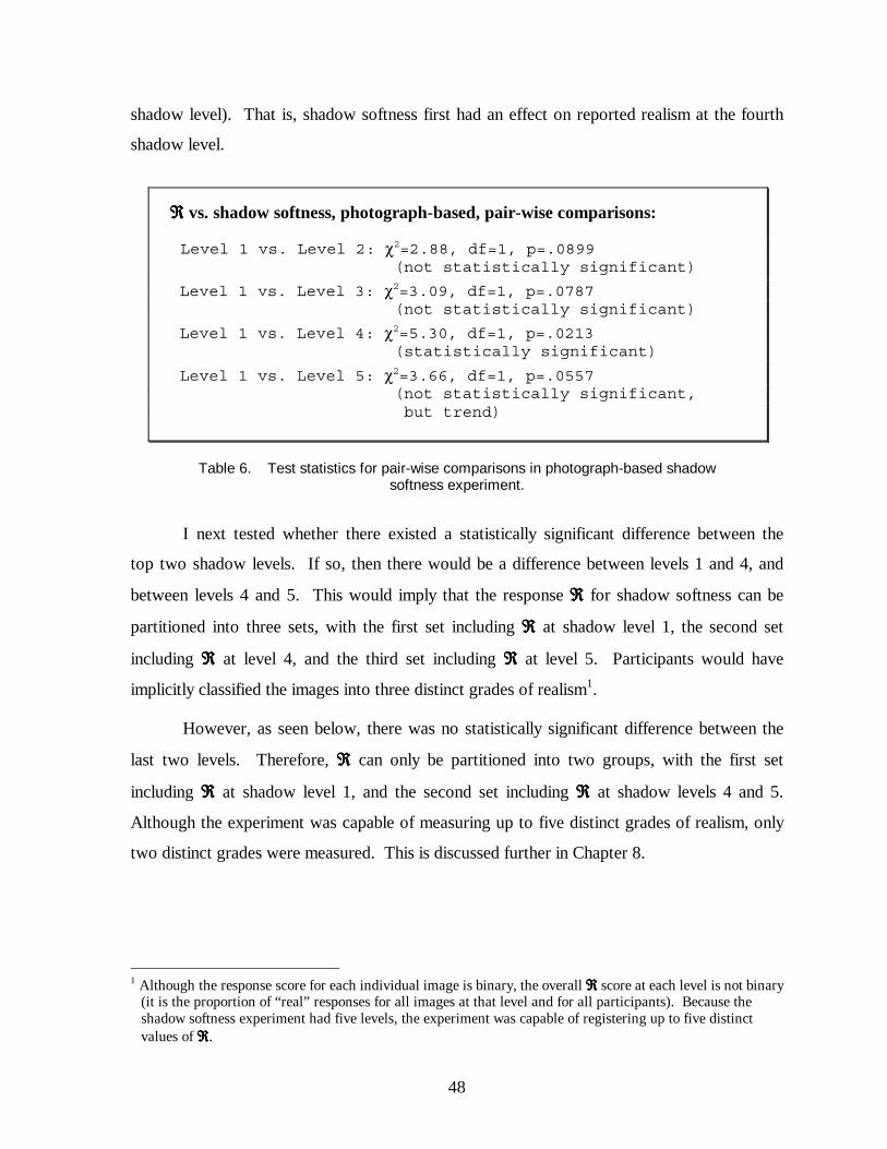
48

shadow level). That is, shadow softness first had an effect on reported realism at the fourth

shadow level.

ℜℜℜℜ vs. shadow softness, photograph-based, pair-wise comparisons:

Level 1 vs. Level 2: χ2=2.88, df=1, p=.0899 (not statistically significant)

Level 1 vs. Level 3: χ2=3.09, df=1, p=.0787 (not statistically significant)

Level 1 vs. Level 4: χ2=5.30, df=1, p=.0213 (statistically significant)

Level 1 vs. Level 5: χ2=3.66, df=1, p=.0557 (not statistically significant, but trend)

Table 6. Test statistics for pair-wise comparisons in photograph-based shadow softness experiment.

I next tested whether there existed a statistically significant difference between the

top two shadow levels. If so, then there would be a difference between levels 1 and 4, and

between levels 4 and 5. This would imply that the response ℜℜℜℜ for shadow softness can be

partitioned into three sets, with the first set including ℜℜℜℜ at shadow level 1, the second set

including ℜℜℜℜ at level 4, and the third set including ℜℜℜℜ at level 5. Participants would have

implicitly classified the images into three distinct grades of realism1.

However, as seen below, there was no statistically significant difference between the

last two levels. Therefore, ℜℜℜℜ can only be partitioned into two groups, with the first set

including ℜℜℜℜ at shadow level 1, and the second set including ℜℜℜℜ at shadow levels 4 and 5.

Although the experiment was capable of measuring up to five distinct grades of realism, only

two distinct grades were measured. This is discussed further in Chapter 8.

1 Although the response score for each individual image is binary, the overall ℜℜℜℜ score at each level is not binary

(it is the proportion of “real” responses for all images at that level and for all participants). Because the shadow softness experiment had five levels, the experiment was capable of registering up to five distinct values of ℜℜℜℜ.

49

ℜℜℜℜ vs. shadow softness, photograph-based, comparison of two softest levels:

Level 4 vs. Level 5: χ2=2.60, df=1, p=.1072 (not statistically significant)

Table 7. Test statistics for comparison of top two levels in photograph-based shadow softness experiment.

5.3 Surface smoothness

5.3.1 Experimental setup

This photograph-based experiment investigated whether perceived visual realism

varies with surface smoothness. Two levels of surface smoothness were tested. Images in

the first level contained smooth-textured cubes, and images in the second level contained

rough-textured cubes. The smooth textures were created using white spray-paint, which gave

a flat, even coat. The rough textures were created by painting with white paint and a rough-

bristled brush, which produced uneven brush marks with paint at varying heights. Because

the objects were completely painted white, the visible variations on the surfaces were due

only to shading differences from the undulating surface normals. There were 30 images for

each of the two surface smoothness levels.

50

Figure 10. Detail of two images from photograph-based surface smoothness experiment. The smooth, spray-painted cubes (left) rated much

lower in realism than the rough, brush-painted cubes (right).

5.3.2 Results: ℜℜℜℜ vs. surface smoothness

The photograph-based surface smoothness experiment was performed with eighteen

participants. Table 1 shows which participants performed this experiment. The graph below

shows the results, presented as ℜℜℜℜ vs. surface smoothness. There was a strong difference in

reported realism for the two types of surfaces. The rough-painted cubes were rated much

higher than the smooth-painted ones (ℜℜℜℜ = .71 vs. ℜℜℜℜ = .39).

ℜℜℜℜ

Smooth Rough0.1

0.2

0.3

0.4

0.5

0.6

0.7

0.8

0.9

Surface Type

Figure 11. ℜℜℜℜ vs. surface smoothness for photographic experiment. Images with rough textures rated much higher (statistically

significant) than images with smooth textures.

51

I tested for statistical significance using surface smoothness as an independent

variable (with two levels, “smooth” and “rough”). The null hypothesis was that surface

smoothness has no effect on participants’ responses. The full logistic regression model is

given in Table 3.

The effect of surface smoothness was statistically significant, as shown below. This

indicates that surface smoothness had a measurable effect on participants’ responses. The

implications of this finding with respect to visual realism are discussed in Chapter 8.

ℜℜℜℜ vs. surface smoothness, photograph-based,

binary independent variable: SURFACE: χ2=12.85, df=1, p=.0003 (statistically significant)

Table 8. Test statistics for photograph-based surface smoothness experiment.

5.4 Interaction effects between shadow softness and surface smoothness

As described at the beginning of this chapter, shadow softness and surface

smoothness were varied simultaneously within a single experiment. The previous two

sections discussed the main effects of shadow softness and surface smoothness. That is, the

difference in ℜℜℜℜ between the five shadow softness levels (with the two levels of surface

smoothness taken together), and the difference in ℜℜℜℜ between the two surface smoothness

levels (with the five levels of shadow softness taken together). However, it is possible that

the effect of one factor varies for different individual levels of the other factor. For example,

it could be the case that the effect of shadow softness is different for rough surfaces than for

smooth surfaces.

The presence of an interaction effect does not affect the statistical analysis of the

main effects of the experiment, but it does affect the interpretation and discussion of results:

for a given image, the effect of one factor cannot be predicted without considering the level

of the other factor. When there is no interaction, the effect of one factor can be predicted for

a given image without consideration of the other factor.

52

The full logistic regression model is given in Table 3. The result for interaction

between shadow softness and surface smoothness is:

ℜℜℜℜ vs. interaction between surface smoothness and shadow softness,

photograph-based: SURFACE × SHADOW: χ2=0.14, df=1, p=.7102 (not statistically significant)

Table 9. Test statistics for interaction between surface smoothness and shadow softness in photograph-based experiment.

The analysis shows that there was no statistically significant interaction between

surface smoothness and shadow softness. The effect on perceived visual realism of one

factor did not depend on the level of the other factor. That is, shadow softness had the same

effect on perceived visual realism regardless of the smoothness of surfaces, and surface

smoothness had the same effect on perceived visual realism regardless of the softness of

shadows.

6. PHOTOGRAPH-BASED EXPERIMENTS ON NUMBER OF OBJECTS, MIX OF OBJECT SHAPES, AND

NUMBER OF LIGHT SOURCES

This chapter reports on photograph-based experiments investigating the effect of

number of objects, mix of object shapes, and number of light sources on perceived visual

realism. Number of objects and mix of object shapes were studied in a combined two-factor

experiment. Number of light sources was studied independently, in a single-factor

experiment.

6.1 Number of objects and mix of object shapes

6.1.1 Experimental setup

The effects of number of objects and mix of object shapes were tested simultaneously

in a single, combined experiment. By testing the two factors together, we are able to test for

an interaction effect between the two. That is, to test whether the number of objects in an

image influences the effect of mix of object shapes, and vice versa.

The logistic regression model for this experiment is:

y = β0 + β1 ∗ NUM_OBJS

+ β2 ∗ MIX_SHAPES

+ β3 ∗ NUM_OBJS ∗ MIX_SHAPES

Table 10. Logistic regression model for experiment on number of objects and mix of object shapes.

54

The statistics presented in this chapter result from the full model given above. For

clarity, the statistics for each main effect and for the interaction effect will be presented in

separate sections.

Nine participants performed this two-factor experiment (see Table 1). The first factor

was the number of objects: each image contained either two, four, eight, or thirty objects.

The second factor was the mix of object shapes, with two levels: each image consisted either

of only cubes, or of half cubes and half rounded objects (spheres and egg-shapes). Crossing

the two factors yielded 4 × 2 = 8 conditions. For example, a given image might have eight

objects that are all cubes, or it might have thirty objects with mixed shapes (fifteen cubes and

fifteen rounded objects). There were five different spatial arrangements of objects for each

of these combinations. The total number of images in this experimental set was therefore 4 ×

2 × 5 = 40.

The order of image presentation was randomized for each participant at run-time.

The light intensity and angle was identical for all the photographs, though half of the images

were displayed flipped horizontally (randomized at run-time per participant). Each

participant initially viewed and rated sixteen practice images, selected randomly from the

experimental set. The data from the practice trials is not included in the analysis. The

images used for the practice trials were used again for the main trials.

55

Figure 12. Sample images from experiment on number of objects and mix of object shapes. The number of objects increases across columns, and the mix of object

shapes (cubes-only versus cubes and rounded objects) varies between rows.

6.1.2 Results: ℜℜℜℜ vs. number of objects

The graphs below show the data, presented as ℜℜℜℜ vs. number of objects. It shows an

overall decrease in ℜℜℜℜ as the number of objects was increased.

Number of Objects

Figure 13. Results of photograph-based experiment on number of objects. There was no statistically significant effect. Note: the x-axis is not evenly scaled.

56

I first tested for statistical significance by fitting a logistic regression model (see

Table 10) to the data using the number of objects in each image (2, 4, 8, and 30) as an

independent variable. The null hypothesis was that number of objects has no effect on

participants’ responses. With this model, number of objects was found to be not statistically

significant (p=.1261). This indicates that ℜℜℜℜ did not increase linearly with the number of

objects in the images.

I next tested whether a better model would offer a statistically significant fit. The

values of the independent variable (2, 4, 8, and 30) were not evenly spaced, but increased

nearly as powers of two. To account for this, I transformed the independent variable using

the log2 function, yielding the values 1, 2, 3, and 4.9. The dependent variable was not

changed by the transformation. With this model, the regression analysis yielded p=.0772,

which indicates a trend, though not statistical significance.

ℜℜℜℜ vs. number of objects, photograph-based, number of objects as independent variable:

NUM_OBJS: χ2=2.34, df=1, p=.1261

(not statistically significant)

ℜℜℜℜ vs. number of objects, photograph-based, log2(number of objects) as independent variable:

NUM_OBJS: χ2=3.12, df=1, p=.0772

(not statistically significant, but trend)

Table 11. Test statistics for photograph-based experiment on number of objects.

There was no statistically significant overall regression using either model. Reported

realism was therefore not a measurable function of either number of objects or log2 number

of objects.

I next performed pair-wise tests to see if there were measurable differences between

the first level and each additional level. As presented below, there was a statistically

significant difference between levels 1 and 2, and between levels 1 and 4. However, there

57

was no difference between levels 1 and 3. Although there were differences between

individual pairs, the overall regression was not statistically significant because of the value of

ℜℜℜℜ at the third level. Future experiments with more participants could determine whether this

was due to low power, since more participants could potentially yield a smoother response

curve.

Because the overall regression for number of objects was not statistically significant,

I did not investigate how many distinct grades of realism were evoked, as I did for the

shadow softness experiment in Chapter 5.

The implications of these findings with respect to visual realism are discussed in

Chapter 8.

ℜℜℜℜ vs. number of objects, photograph-based, pair-wise comparisons:

Level 1 vs. Level 2: χ2=4.25, df=1, p=.0392 (statistically significant)

Level 1 vs. Level 3: χ2=1.91, df=1, p=.1674 (not statistically significant)

Level 1 vs. Level 4: χ2=4.74, df=1, p=.0295 (statistically significant)

Table 12. Test statistics for pair-wise comparisons in photograph-based experiment on number of objects.

6.1.3 Results: ℜℜℜℜ vs. mix of object shapes

The mix of object shapes was co-varied along with the number of objects, as

described at the beginning of this chapter. Mix of object shapes was tested with two levels:

each image either showed only blocks, or showed an equal mix of blocks and rounded

objects. The graph below shows the results, presented as ℜℜℜℜ vs. mix of object shapes.

58

Mix of Object Shapes

Figure 14. Results of photograph-based experiments on mix of object shapes. There was no statistically significant effect.

The graph shows that there was not much difference in ℜℜℜℜ between the two levels. I

tested for statistical significance by fitting a logistic regression model (see Table 10) to the

data, using mix of object shapes as an independent variable (with two levels, “mixed” and

“not mixed”). The null hypothesis was that mix of object shapes has no effect on

participants’ responses. As shown below, the regression test was not statistically significant.

Participants’ responses did not vary based on whether an image displayed only objects of the

same shape, or objects of mixed shapes.

ℜℜℜℜ vs. mix of object shapes, photograph-based, binary independent variable:

MIX_SHAPES: χ2=0.56, df=1, p=.4550 (not statistically significant)

Table 13. Test statistics for photograph-based experiment on mix of object shapes.

6.1.4 Interaction between number of objects and mix of object shapes

Because the two factors were tested simultaneously in a single experiment, we can

test for interaction between them. The analysis is given below. The interaction term is not

statistically significant. This implies that the effect of each factor did not depend on the

current level of the other factor.

59

ℜℜℜℜ vs. interaction between number of objects and mix of object shapes, photograph-based:

NUM_OBJS × MIX_SHAPES: χ2=0.02, df=1, p=.8862 (not statistically significant)

Table 14. Test statistics for interaction between number of objects and mix of object shapes.

6.2 Number of light sources

6.2.1 Experimental setup

This experiment investigated whether perceived visual realism varies with number of

light sources. There were three levels of this factor: scenes were lit with either one, two, or

four lights. There was an additional crossed factor, shadow softness, with two levels: hard

and soft shadows. The hard-shadowed images were created using the spotlight from the

photograph-based shadow softness experiment in Chapter 5 (shadow softness level 1), and

the soft-shadowed images were created using the diffuse light from that experiment (shadow

softness level 5).

The logistic regression model for this experiment is:

y = β0 + β1 ∗ NUM_LIGHTS

+ β2 ∗ SHADOWNUM_LIGHTS_EXP

+ β3 ∗ NUM_LIGHTS ∗ SHADOWNUM_LIGHTS_EXP

Table 15. Logistic regression model for experiment on number of light sources.

There were six possible lighting conditions in this experiment (number of lights ×

shadow softness = 3 × 2). This experiment also used six spatial arrangements of objects.

The total number of images in this experiment was therefore 3 × 2 × 6 = 36. Half of these

images (randomized per participant) were displayed flipped horizontally. Each participant

initially viewed and rated sixteen practice images, selected randomly from the experimental

60

set. The data from the practice trials is not included in the analysis. The images used for the

practice trials were used again for the main trials.

6.2.2 Creation of images

The images in this experiment were generated by blending photographs containing a

single light source each. This section describes the creation of images with one, two, and

four light sources, for a single shadow softness level and a single scene. The procedure was

repeated for the two shadow softness levels, across the six scenes.

A single light source was placed at four evenly-spaced locations along a 120° arc

around the given scene. For each of the four light source locations, a photograph of the scene

was taken. The camera location was held constant, and operated via remote control. The

aperture and exposure settings were locked for all the photographs.

The photographs, which were each lit by a single light, were blended to generate

images that appeared to contain multiple light sources. For example, to generate an image

with two light sources, two light positions were randomly selected and the two corresponding

images were blended to create a single new image that appeared to be lit by two lights. The

image selection and blending process was automated by a custom software utility.

The blend operation was radiometrically correct. I used the mkhdr software tool

([Diuk98], based on [Debe97]) to calculate the CCD response curve of the digital camera

used in this experiment. Given a set of images of a fixed scene at different exposure levels,

mkhdr calculates a scale-less response curve. This response curve provides a mapping

between photometric values (luminance) and camera pixels. Based on the response curve of

the camera used in this experiment, the formula used to compute photometric luminance

values from camera pixel values was:

photometric_luminance =

.2545 − .0053 ∗ camera_pixel_value +

.000085 ∗ camera_pixel_value ∗ camera_pixel_value

61

To blend a pair of images with different light locations, each image is first mapped

into photometric space (mapped from camera pixel intensities to luminance). Due to the

additive nature of light, the luminance field from two simultaneous light sources is equivalent

to the sum of the luminance fields from each independent light source. To simulate two

simultaneous light sources, the two photometric-space images (each containing a single light

source) are summed. The resulting image is overexposed by a factor of two relative to the

original photographs, so the exposure is reduced by multiplying the intensity values by one-

half. Finally, the image is mapped back to camera-pixel space using the inverse of the

function above. The resulting image represents what a photograph would look like had it

been taken with the two light sources simultaneously, at one-half the exposure time of the

original photographs.

When multiple images are blended, the resulting image has less camera noise than the

original images. The camera noise can be modeled as a random variable across the image,

with some expected value E. As the number of images that are blended increases, the camera

noise for each pixel of the resulting image goes to the expected value E, and the random

variation decreases. To prevent camera noise from decreasing as the number of blended

images increases (which would confound the analysis) each image in the experiment was

created by blending exactly four single-light-source photographs.

To accomplish this, I took four photographs for each of the four light source positions

(i.e., 4 × 4 = 16 photographs per scene). Four photographs with the same light position were

blended to generate an image with “one” light. Two pairs of photographs, with the same

light position within each pair, were blended to generate an image with “two” lights. Four

photographs, each with a different light position, were blended to generate an image with

“four” lights. Because each new image was a blend of exactly four images, they all had the

same amount of camera noise. Camera noise was therefore not a confounding factor.

62

Figure 15. Sample images from experiment on number of light sources. From left to right, images have one, two, and four light sources. Top row has hard

shadows; bottom row has soft shadows. There was no statistically significant effect with respect to number of light sources.

6.2.3 Results: ℜℜℜℜ vs. number of light sources

Six participants performed the experiment on number of light sources. Table 1 shows

which participants performed this experiment. The graph below shows the resulting data,

presented as ℜℜℜℜ vs. number of light sources. There was a decrease in reported realism as the

number of lights was increased.

ℜℜℜℜ

Number of Light Sources

Figure 16. Results of photograph-based experiment on number of light sources. There was no statistically significant effect

63

I first tested for statistical significance by fitting a logistic regression model (see

Table 15) to the data using the number of lights (1, 2, and 4) and the shadow softness (binary:

“soft” vs. “hard”) as the independent variables. The null hypothesis was that number of

lights and shadow softness has no effect on participants’ responses. As shown in the table

below, shadow softness was statistically significant (p=.0071), which is consistent with the

shadow softness results of Chapter 5. However, number of lights was not statistically

significant (p=.4850).

I next tested whether a better model would offer a statistically significant fit with

respect to number of lights. The values of the independent variable (1, 2, and 4) are not

evenly spaced, but increase as powers of two. To account for this, I transformed the

independent variable using the log2 function, yielding the values 1, 2, and 3. The dependent

variable was not changed by the transformation. With this model, the regression analysis

yielded p=.4790, which is still not statistically significant.

I also tested the interaction term between number of lights and shadow softness. This

was not statistically significant (p=.3544). This indicates that participants’ responses with

respect to number of lights did not vary according to the current shadow softness level, nor

vice versa. The two were independent.

Lastly, I conducted pair-wise tests between the three levels of number of lights. The

tests were not statistically significant, which indicates that there were no differences amongst

the individual levels. This, along with the lack of overall statistical significance, indicates

that only a single grade of realism was detected with respect to number of light sources.

The implications of these results are discussed in Chapter 8.

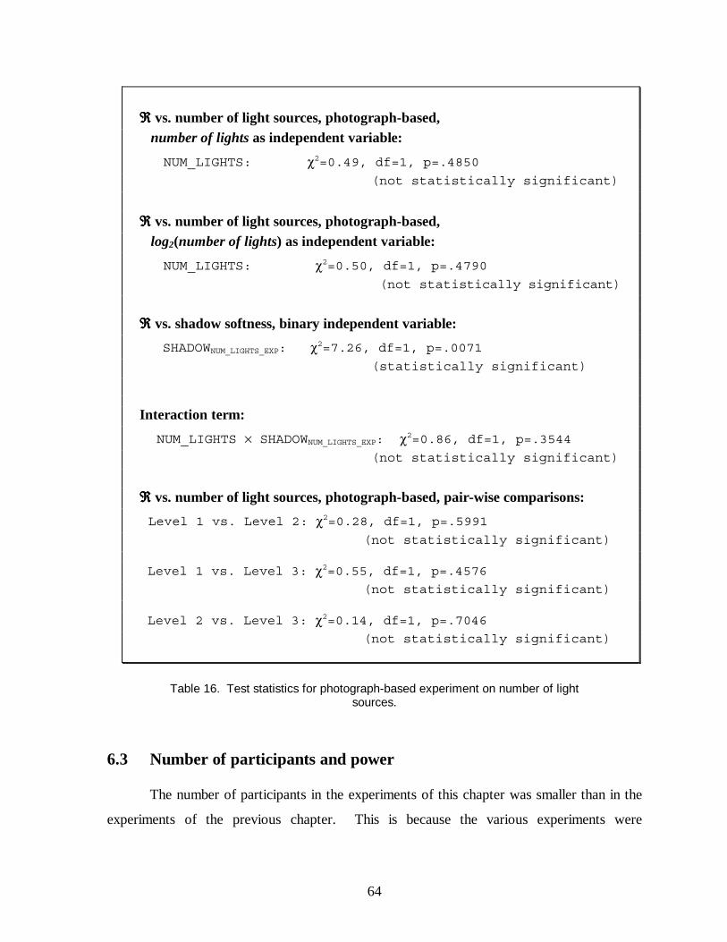
64

ℜℜℜℜ vs. number of light sources, photograph-based, number of lights as independent variable:

NUM_LIGHTS: χ2=0.49, df=1, p=.4850

(not statistically significant)

ℜℜℜℜ vs. number of light sources, photograph-based, log2(number of lights) as independent variable:

NUM_LIGHTS: χ2=0.50, df=1, p=.4790

(not statistically significant)

ℜℜℜℜ vs. shadow softness, binary independent variable:

SHADOWNUM_LIGHTS_EXP: χ2=7.26, df=1, p=.0071

(statistically significant)

Interaction term:

NUM_LIGHTS × SHADOWNUM_LIGHTS_EXP: χ2=0.86, df=1, p=.3544

(not statistically significant)

ℜℜℜℜ vs. number of light sources, photograph-based, pair-wise comparisons:

Level 1 vs. Level 2: χ2=0.28, df=1, p=.5991

(not statistically significant)

Level 1 vs. Level 3: χ2=0.55, df=1, p=.4576

(not statistically significant)

Level 2 vs. Level 3: χ2=0.14, df=1, p=.7046

(not statistically significant)

Table 16. Test statistics for photograph-based experiment on number of light sources.

6.3 Number of participants and power

The number of participants in the experiments of this chapter was smaller than in the

experiments of the previous chapter. This is because the various experiments were

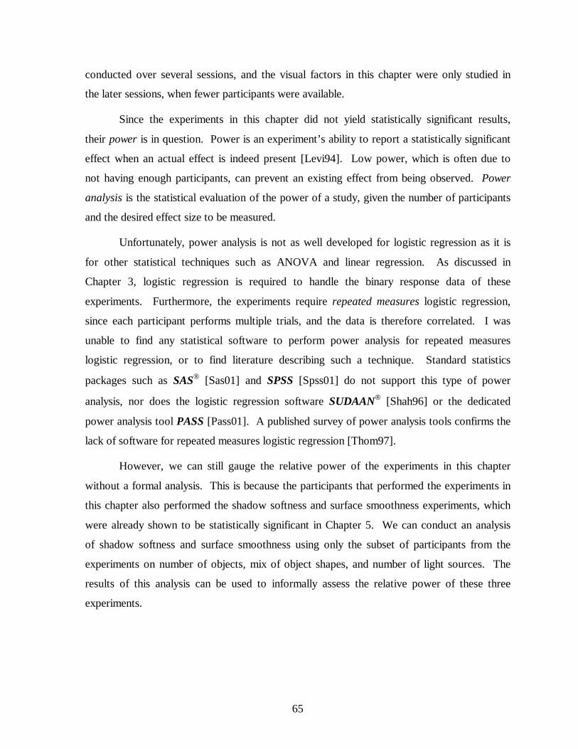
65

conducted over several sessions, and the visual factors in this chapter were only studied in

the later sessions, when fewer participants were available.

Since the experiments in this chapter did not yield statistically significant results,

their power is in question. Power is an experiment’s ability to report a statistically significant

effect when an actual effect is indeed present [Levi94]. Low power, which is often due to

not having enough participants, can prevent an existing effect from being observed. Power

analysis is the statistical evaluation of the power of a study, given the number of participants

and the desired effect size to be measured.

Unfortunately, power analysis is not as well developed for logistic regression as it is

for other statistical techniques such as ANOVA and linear regression. As discussed in

Chapter 3, logistic regression is required to handle the binary response data of these

experiments. Furthermore, the experiments require repeated measures logistic regression,

since each participant performs multiple trials, and the data is therefore correlated. I was

unable to find any statistical software to perform power analysis for repeated measures

logistic regression, or to find literature describing such a technique. Standard statistics

packages such as SAS [Sas01] and SPSS [Spss01] do not support this type of power

analysis, nor does the logistic regression software SUDAAN [Shah96] or the dedicated

power analysis tool PASS [Pass01]. A published survey of power analysis tools confirms the

lack of software for repeated measures logistic regression [Thom97].

However, we can still gauge the relative power of the experiments in this chapter

without a formal analysis. This is because the participants that performed the experiments in

this chapter also performed the shadow softness and surface smoothness experiments, which

were already shown to be statistically significant in Chapter 5. We can conduct an analysis

of shadow softness and surface smoothness using only the subset of participants from the

experiments on number of objects, mix of object shapes, and number of light sources. The

results of this analysis can be used to informally assess the relative power of these three

experiments.

66

ℜℜℜℜ ℜℜℜℜ

Penumbra Angle Surface Type

Figure 17. Graphs of shadow softness and surface smoothness responses, using data from nine participants that also performed experiments on number of objects

and mix of object shapes.

ℜℜℜℜ vs. shadow softness and surface smoothness (photograph-based), using only the nine participants that performed experiments on number of objects and mix of object shapes:

SHADOW: χ2=0.82, df=1, p=.3665 (not statistically significant) SURFACE: χ2=15.64, df=1, p<.0001 (statistically significant)

Table 17. Test statistics for photograph-based shadow softness and surface smoothness experiments, using data from nine participants that also performed

experiments on number of objects and mix of object shapes.

ℜℜℜℜ

ℜℜℜℜ

Penumbra Angle Surface Type

Figure 18. Graphs of shadow softness and surface smoothness responses, using data from six participants that also performed experiment on number of light

sources.

67

ℜℜℜℜ vs. shadow softness and surface smoothness (photograph-based), using only the six participants that performed experiment on number of light sources:

SHADOW: χ2=3.95, df=1, p=.0470 (statistically significant) SURFACE: χ2=8.12, df=1, p=.0044 (statistically significant)

Table 18. Test statistics for photograph-based shadow softness and surface smoothness experiments, using data from six participants that also performed

experiment on number of light sources.

Table 17 shows that the surface smoothness experiment from Chapter 5 was

statistically significant when using only the participant set that also performed the combined

experiment on number of objects and mix of object shapes. The participant set from the

experiment on number of objects and mix of object shapes therefore yielded enough power

for an effect of the magnitude of surface smoothness to be detected. Since number of objects

and mix of object shapes were not statistically significant with these same participants, we

can infer that these two factors influenced perceived visual realism less than surface

smoothness did.

The shadow softness experiment from Chapter 5 was not statistically significant using

the participant set that also performed the combined experiment on number of objects and

mix of object shapes. We therefore cannot determine whether shadow softness had more or

less influence than number of objects or mix of object shapes.

Table 18 shows that both the shadow softness and the surface smoothness

experiments from Chapter 5 were statistically significant using the participant set that also

performed the experiment on number of light sources. The participant set from the

experiment on number of light sources therefore yielded enough power for an effect of the

magnitude of both shadow softness and surface smoothness to be detected. Since number of

light sources was not statistically significant with these same participants, we can infer that

number of light sources had less influence than either shadow softness or surface

smoothness.

7. EXPERIMENTS USING COMPUTER-GENERATED IMAGES

The experiments presented in the previous two chapters used only photographs. It

would be useful to know whether the experimental method is also valid for computer-

generated images.

Photographs limit the kinds of visual factors that can be investigated. Non-

physically-realistic effects cannot be studied using unmanipulated photographs. For

example, with photographs one cannot arbitrarily manipulate the propagation of light

throughout a scene, as one can with computer graphics. Computer graphics are not bound by

physical correctness, and can be used to create images that would be impossible with

unmanipulated photography.

Photographs also limit the experimental control that can be achieved across images.

This problem was noted in the experiment on shadow softness in Chapter 5, where different

lighting conditions were required to generate the different shadow levels, and this led to

variations in image brightness and contrast. With computer graphics, images can be

generated with precise experimental control across the various visual factors.

The goal of this chapter is to determine whether CG-based experiments produce

results that are consistent with photograph-based experiments. In this chapter we test this by

conducting experiments on shadow softness and surface smoothness using only computer-

generated images. The results from these experiments will be compared to the photograph-

based shadow softness and surface smoothness experiments from Chapter 5.

69

7.1 Setup

The computer-generated images for this experiment were rendered using 3D Studio

Max [Disc02]. Soft shadows were generated by raycasting towards a disc light source of

varying radius. The radius of the light source affected only the softness of the shadow

penumbras. The illumination on non-penumbral regions was not affected by changes in the

light source radius. This is an example of the control afforded by computer graphics.

Object textures were created using orthographic photographs of the physical cubes

used in the photograph-based experiments. The intensity values of the resulting textures

were shifted to a common mean, to ensure they all had the same average intensity. The

textures were used as bump maps [Blin78], rather than as reflectance maps. The same anti-

aliasing algorithm (a quadratic filtering kernel) was used for all the images; anti-aliasing was

therefore a controlled factor.

The images were rendered with direct lighting only, and lacked indirect illumination

(i.e., reflectance of light from surfaces onto other surfaces was not computed). It is possible

that CG images without indirect illumination would be judged as less real than their

photographic counterparts, if a side-by-side comparison were performed. However, the

baseline realism of the set of images is not important in this experimental design. The only

question is whether realism measurably increases or decreases across the levels of the

manipulated factors. The lack of indirect illumination does not present a problem as long as

it does not overpower the effects of shadow softness and surface smoothness, causing a floor

effect (i.e., as long as the images are not all rated as “not real” because of it).

Unlike the photograph-based shadow softness experiment from Chapter 5, the lowest

shadow level in the CG-based experiment had a penumbra angle of zero degrees – a perfect

point light source. Point light sources are not possible in the real world, but they are

common in computer graphics. Here we test their effect on perceived realism.

Seven participants performed the CG-based shadow softness and surface smoothness

experiments. Table 1 shows which participants performed the CG-based experiments. To

eliminate the possibility of crossover effects from exposure to both CG images and

70

photographs, the participants in these CG-based experiments were different from those that

performed the photograph-based experiments.

Unlike the photograph-based shadow softness and surface smoothness experiments,

the CG-based factors were tested in two independent experiments. We therefore cannot

perform a test for interaction between the two CG-based factors.

Shadow softness was tested with five shadow levels (at 0, 1.5, 2.5, 5.2, and 10.3

degrees of penumbra angle) and with six different spatial arrangements of objects. The total

number of images for the shadow softness experiment was therefore 5 × 6 = 30. Surface

smoothness was tested with two smoothness levels, and with twelve different spatial

arrangements of objects. The total number of images for the surface smoothness experiment

was therefore 2 × 12 = 24. The logistic regression models for the two experiments are

presented below:

y = β0 + β1 ∗ SHADOWCG

Table 19. Logistic regression model for CG-based experiment on shadow softness.

y = β0 + β1 ∗ SURFACECG

Table 20. Logistic regression model for CG-based experiment on surface smoothness.

Half of the images in the experiments (randomized per participant at run-time) were

displayed flipped horizontally. Each participant initially viewed and rated sixteen practice

images, selected randomly from the experimental set. The data from the practice trials is not

included in the analysis. The images used for the practice trials were used again for the main

trials.

71

Figure 19. Sample images from computer-graphics-based shadow softness experiment. Shadow softness varies across columns, from hardest (left) to softest

(right). Object arrangement varies between rows.

Figure 20. Detail of images from CG-based shadow softness experiment. Average penumbra angles for the five shadow levels were 0°, 1.5°, 2.5°, 5.2°, and 10.3°.

72

Figure 21. Detail of images from CG-based surface smoothness experiment. The bump maps for the computer-generated objects were acquired by photographing the faces of the cubes used in the photograph-based surface smoothness experiment.

7.2 Results: ℜℜℜℜ vs. shadow softness (computer-graphics-based experiment)

The reported realism rating ℜℜℜℜ increased with shadow softness, as it did in the

photographic experiment presented in Chapter 5. This is shown in the graph below.

However, the change in ℜℜℜℜ between the first and second shadow levels was more pronounced

with computer graphics than with photographs. This may be due to the fact that the CG

renderings contained a true point light source, which cannot be achieved with a physical

spotlight. The lowest shadow softness level in the CG images was therefore less physically

plausible than the lowest level in the photograph-based experiment.

73

Penumbra Angle

Figure 22. Results of computer-graphics-based experiment on shadow softness. There was a statistically significant increase in ℜℜℜℜ. The greatest increase in reported

realism occurred between the first and second levels.

I first tested whether ℜℜℜℜ varied linearly with shadow softness by fitting a logistic

regression model (see Table 19) to the data, using degrees of penumbra angle as the

independent variable. The null hypothesis was that shadow softness has no effect on

participants’ responses. With this model, shadow softness was found to be not statistically

significant (p=.0863, a trend). As with the photographic shadow softness experiment, ℜℜℜℜ did

not vary linearly with degrees of penumbra angle.

I next tested whether a better model would offer a statistically significant fit, noting

that the penumbra angle values were not evenly spaced, but rather increased exponentially (0,

1.5, 2.5, 5.2, and 10.3). To account for this, I transformed the independent variable using the

function log2(α + 1.0), where α is the degrees of penumbra angle. I used (α + 1.0) instead of

just α (as in the photographic analysis) because log2(0) is undefined, and the lowest shadow

level has a penumbra angle of zero.

After the transformation, the independent variable took the following values: 0, 1.33,

1.8, 2.6, and 3.5. The dependent variable was not changed by the transformation. With this

model, the regression was statistically significant, with p=.0228. This indicates that ℜℜℜℜ

increased measurably with log2 degrees of penumbra angle, for CG-based shadow softness.

This is consistent with the findings from the photograph-based experiment.

74

ℜℜℜℜ vs. shadow softness, CG-based,

degrees of penumbra angle as independent variable:

SHADOWCG: χ2=2.94, df=1, p=.0863

(not statistically significant, but trend)

ℜℜℜℜ vs. shadow softness, CG-based:

log2(degrees of penumbra angle + 1.0) as independent variable:

SHADOWCG: χ2=5.18, df=1, p=.0228

(statistically significant)

Table 21. Test statistics for computer-graphics-based experiment on shadow softness.

Because there were more than two levels of shadow softness, we can perform pair-

wise tests for the log2 case to determine at which level, relative to the first, the effect

becomes statistically significant. As presented in the table below, a statistically significant

difference in ℜℜℜℜ first appears between shadow levels 1 and 2.

ℜℜℜℜ vs. shadow softness, CG-based, pair-wise comparisons,

log2(degrees of penumbra angle + 1.0) as independent variable:

Level 1 vs. Level 2: χ2=6.64, df=1, p=.0100 (statistically significant)

Level 1 vs. Level 3: χ2=2.30, df=1, p=.1296 (not statistically significant)

Level 1 vs. Level 4: χ2=7.34, df=1, p=.0068 (statistically significant)

Level 1 vs. Level 5: χ2=5.14, df=1, p=.0234 (statistically significant)

Table 22. Test statistics for pair-wise comparisons in computer-graphics-based experiment on shadow softness.

As with the photograph-based shadow softness experiment in Chapter 5, we can now

test whether participants implicitly classified the images into more than two distinct grades of

75

realism. We can explore this by testing levels 2 through 5, and if these exhibit statistical

significance, then we proceed to test for pair-wise differences starting at level 2.

I ran a logistic regression test including only levels 2 through 5, with log2 shadow

softness as the independent variable. The null hypothesis was that shadow softness has no

effect on reported realism.

As shown below, there was no statistically significant difference in the last four

shadow softness levels. We therefore do not proceed to conduct further pair-wise

comparisons, but instead conclude that ℜℜℜℜ can only be partitioned into two groups, with the

first set including ℜℜℜℜ at shadow level 1, and the second set including ℜℜℜℜ at shadow levels 2

through 5. Although the experiment was capable of measuring up to five distinct grades of

realism, only two distinct grades were measured. This is discussed further in Chapter 8.

ℜℜℜℜ vs. shadow softness, CG-based, comparison of four softest levels

log2(degrees of penumbra angle + 1.0) as independent variable:

Levels 2, 3, 4, 5: χ2=0.35, df=1, p=.5562

(not statistically significant)

Table 23. Test statistics for comparison of last four levels in computer-graphics-based shadow softness experiment.

7.3 Results: ℜℜℜℜ vs. surface smoothness (computer-graphics-based experiment)

As shown in the graph below, smooth-surfaced images rated much lower in ℜℜℜℜ than

rough-surfaced images. This is consistent with the results from the photograph-based surface

smoothness experiment.

76

Surface Type

Figure 23. Results of computer-graphics-based experiment on surface smoothness. These closely match the results from the photograph-based

experiment. The increase in ℜℜℜℜ was statistically significant.

I tested for statistical significance by fitting a logistic regression model (see Table 20)

to the data, using surface smoothness as the independent variable (with two levels, “smooth”

and “rough”). The null hypothesis was that surface smoothness has no effect on participants’

responses.

The effect of surface smoothness was statistically significant, as shown below. This

indicates that surface smoothness had a measurable effect on participants’ responses.

ℜℜℜℜ vs. surface smoothness, CG-based, binary independent variable:

SURFACECG: χ2=18.75, df=1, p<.0001 (statistically significant)

Table 24. Test statistics for computer-graphics-based experiment on surface smoothness.

7.4 Comparison of photograph-based and computer-graphics-based shadow softness and surface smoothness experiments

The results of the computer-graphics based shadow softness and surface smoothness

experiments are consistent with the photograph-based experiments presented in Chapter 5.

77

There was a statistically significant increase in the realism response as shadows were

softened and as surfaces were made less smooth.

Shadow softness

(log2 degrees of penumbra angle) Surface smoothness

(“smooth” vs. “rough” textures)

Photograph-based

experiments χ2=4.32, df=1, p=.0377 χ2=12.85, df=1, p=.0003

CG-based experiments χ2=5.18, df=1, p=.0228 χ2=18.75, df=1, p<.0001

Table 25. Test statistics for photograph-based and computer-graphics-based experiments on shadow softness and surface smoothness.

In both the photograph-based and CG-based shadow softness experiments, it was

found that the realism response did not increase linearly with penumbra angle, but instead

increased with log2 of penumbra angle.

Also, the realism response increased quickly with shadow softness and then leveled

off, in both the photograph-based and CG-based experiments. Statistical analysis determined

that only two distinct grades of realism were reported in both of these experiments, despite

the fact that the experiments were capable of measuring up to five distinct grades of realism

(one per level of shadow softness).

8. DISCUSSION

I have presented a novel experimental method for measuring the perceived visual

realism of images. This method differs from existing research on visual realism in that it is

the first to ask human participants to directly rate images as either “real” or “not real.” The

experimental method presents participants with a series of images that vary only along

specific manipulated factors. Statistical analysis is used to determine whether the

manipulated factors had an effect on participants’ responses. By seeing which visual factors

had an effect on reported realism and which did not, we can learn what is visually important

for an image to be regarded as “real.”

8.1 Experimental results

I conducted experiments on the following five visual factors: shadow softness,

surface smoothness, number of objects, mix of object shapes, and number of light sources.

8.1.1 Discussion: shadow softness and surface smoothness

Shadow softness was tested with both photograph-based and CG-based experiments.

Participants viewed images with very hard shadows (from a spotlight), very soft shadows

(from a diffused light source), and three intermediate levels of shadow softness. In both the

photograph-based and CG-based experiments, the realism response ℜℜℜℜ was lower for hard

shadows than for soft shadows. The effect was statistically significant. This indicates that

participants consistently rated soft-shadowed images as “real” more often than they did hard-

shadowed images. Shadow softness therefore measurably increased perceived visual realism.

ℜℜℜℜ was defined in each experiment as the proportion of images that were rated as

“real” at a given level of the visual factor (in this case, at a given level of shadow softness).

79

The ℜℜℜℜ curve increased quickly with shadow softness at only a few degrees of penumbra

angle, and then leveled off. The increase in ℜℜℜℜ was not linear with penumbra angle, but rather

logarithmic. The practical application of this finding is that for a given scene there may be

an optimal degree of shadow softness that will maximize perceived visual realism, beyond

which any increase in shadow softness will have diminishing results.

In the CG-based experiment, the increase in ℜℜℜℜ between the first two shadow softness

levels was greater than the increase in ℜℜℜℜ between the first two levels in the photographic

experiment. This may have been because the computer-generated images at the first shadow

softness level contained a perfect point light source. This was trivial to implement using

computer graphics, though it cannot be accomplished in photographs using physical

spotlights. The first CG shadow softness level was therefore less physically plausible than

the first photographic shadow softness level.

In the CG-based experiment, the greatest increase in ℜℜℜℜ occurred between the first two

shadow softness levels, and there was no statistically significant difference in ℜℜℜℜ between the

four softer shadow levels. Participants effectively divided the images into two groups, where

all the images containing the point light source were rated low on realism, and all the other

images were rated equally high (statistically) on realism. Likewise, the responses in the

photograph-based shadow softness level could only be partitioned into two groups. Despite

the fact that the experiments could measure five distinct grades of perceived visual realism

(one for each of the five levels of shadow softness), only two distinct grades of realism were

measured. Neither the photograph-based nor the CG-based shadow softness experiment

answered the open question of whether people can differentiate between more than two

grades of perceived visual realism1.

Surface smoothness was investigated with both photograph-based and CG-based

experiments. Two levels of surface smoothness were tested: images showed either rough-

surfaced objects or smooth-surfaced objects. For both photographs and computer graphics,

the rough-surfaced images were rated much higher on realism than the smooth-surfaced

1 The other experiments capable of registering more than two levels of perceived visual realism – the

experiments on number of objects and number of light sources – did not yield statistically significant results.

80

images, with statistical significance. This suggests that in order to maximize perceived

visual realism, the surfaces in an image should not all be smooth.

The photograph-based shadow softness and surface smoothness experiments were

investigated in a single combined experiment, to allow for a test for interaction between the

two factors. No statistically significant interaction was found. The effect of shadow softness

did not depend on the current level of surface smoothness, nor vice versa. The two had

independent effects on perceived visual realism.

Both the CG-based shadow softness experiment and the CG-based surface

smoothness experiments were consistent with their photograph-based counterparts, in that

they had similar ℜℜℜℜ response curves, with statistical significance. This demonstrates that the

experimental method presented here can be used with computer-generated images as well as

photographs, which greatly expands the range of possible visual factors that can be studied.

It is often stated within the computer graphics literature that shadow softness and

surface smoothness affect visual realism [Stre95][Sole98][Shir00]. These studies present the

first experimentally obtained evidence that shadow softness and surface smoothness do

indeed have a measurable, statistically significant effect on observers’ regard of images as

being either real or not real.

8.1.2 Discussion: number of objects, mix of object shapes, and number of light sources

Statistically significant effects were not observed for number of objects, mix of object

shapes, or number of light sources. The realism response ℜℜℜℜ did not measurably vary as a

function of any of these three factors (i.e., the slope of the response curve was statistically

zero for all three experiments). This contradicts the common assertion within the computer

graphics literature that complexity implies visual realism [Chiu94][Gree97]. Each of these

three visual factors represented some measure of complexity (though not the only possible

ones), yet none had a statistically significant effect on participants’ responses. The result on

number of objects suggests that if a given image is not realistic, then making it more complex

by replicating the objects within it will not increase its realism. The result on mix of object

shapes suggests that varying the shapes of objects in an image with other objects of similar

geometric and textural complexity will not increase the image’s realism. The result on

81

number of light sources suggests that adding lights to a scene will not affect its perceived

visual realism.

These experiments did not explore the question of why it is that the visual factors did

not have a statistically significant effect on participants’ responses. One possibility is that

the experiments did not have enough power – i.e., there were too few participants and/or the

variance of responses was too large. However, as shown in the informal analysis of power in

Section 6.3, the set of participants for these three visual factors did yield statistical

significance for shadow softness and surface smoothness. It is therefore uncertain whether

conducting these three experiments with more participants would have yielded statistically

significant results. Of the three visual factors, the one most likely to yield different results

with more participants is number of objects, for which a trend was observed (0.1 > p > .05).

8.2 Reliability, sensitivity, and validity

Reliability, sensitivity, and validity [Suth96][Levi94] are relevant issues in the

assessment of novel experimental methods. Reliability is the extent to which an

experimental method gives the same results when employed on different occasions.

Sensitivity refers to the ability of an experimental method to accurately detect an effect,

when one does exist. Validity is the extent to which an experimental method genuinely

measures what it claims to measure.

Reliability is typically measured by performing the experimental tests repeatedly with

the same participants, on different occasions. The method’s reliability is given by the

similarity between the results from different occasions, taking into account that the earlier

exposure to the experimental method may affect the results from the later exposure. I did not

re-test the same participants over time, so the question of whether the experimental results

would be the same upon re-testing remains open for future investigation.

The experimental method exhibited sensitivity, in that it was able to register

statistically significant effects for certain visual factors. This indicates that the experimental

method was able to detect patterns of response for effects of a certain size. Another form of

sensitivity is multi-level sensitivity: the ability to accurately measure different grades of the

response variable. It is not known, however, whether more than two grades of perceived

82

visual realism actually exist. In the two experiments that had statistically significant results

and were capable of registering more than two distinct grades of perceived visual realism,

only two grades of realism were actually measured. These results do not resolve the question

of whether observers are capable of differentiating between more than two grades of

perceived visual realism, and whether multi-level sensitivity is achievable. It is possible that

there exists a single threshold of realism, above which an image is regarded as “real,” and

below which an image is regarded as “not real.”

The question of validity asks whether this experimental method is actually measuring

visual realism. Visual realism is an internal percept, however, and cannot be measured

directly. The only way to assess it is through some external test or observation. The analogy

of intelligence was presented earlier: people believe that intelligence exists, but it can only be

assessed through concrete external means (e.g., intelligence tests) that are believed to

correlate with the abstract internal property. Similarly, the internal perception of visual

realism can only be measured by external means. The external measure in this research is the

question “is this image real?” Perceived visual realism is defined operationally in terms of

this question – a “realistic image” is defined in this research as an image that is rated by

participants as being real. We can therefore assert that the experimental method in this

dissertation provides a valid measure of perceived visual realism of images, where perceived

visual realism is defined operationally as the property of being rated as “real” by human

viewers.

Research works in established fields of perception often address the validity of a new

experimental method by comparing the new method’s results to the results of existing

methods. If the new results are consistent with the existing, accepted results, then the new

method is deemed valid. However, the validity of the method in this dissertation cannot be

evaluated via comparisons with existing methods, since no previous work has attempted to

measure the perceived visual realism of images in a comparable manner (see Chapter 2 for a

full review of the relevant literature).

83

8.3 Results support thesis statement

My thesis statement consisted of three claims. The results of the experiments support

the three claims:

There exist visual factors in images which have measurable, consistent

effects on perceived visual realism, as reported by human observers.

In the photograph-based experiments of Chapter 5, and in the CG-based

experiments of Chapter 7, it was established that shadow softness and

surface smoothness had statistically significant effects on perceived visual

realism, as measured by participants’ responses to the “real” / “not real”

question. Statistical significance indicates that the observed pattern of

responses was not likely due to chance, but rather that a true effect was

likely measured. Statistical significance also indicates that the effect was

consistent across participants: different participants responded similarly to

the manipulated factors.

Not all visual factors have the same effect on perceived visual realism.

Number of objects, mix of object shapes, and number of light sources did

not have statistically significant effects (see Chapter 6). The participants

who performed these three experiments also performed experiments on

shadow softness and surface smoothness, for which their responses were

statistically significant. This demonstrates that not all visual factors have

the same effect on perceived visual realism. For any visual factor that was

not investigated in these experiments, an explicit test will be required to

establish its effect on perceived visual realism.

84

Certain visual factors have similar effects on perceived visual realism in both

photographs and computer-generated images.

Shadow softness and surface smoothness were tested in both photograph-

based and CG-based experiments (in Chapters 5 and 7). The effects were

statistically significant for both photographs and computer-generated

images, and the patterns of responses were qualitatively similar between the

two cases.

8.4 Summary

This research has demonstrated that perceived visual realism can be studied using

standard principles of experimental design and analysis. Realism was defined operationally

in terms of an experimental task. Rather than explicitly defining realism for participants, the

experimental method enabled participants to tell us what they considered real, via their

responses. The presence of statistically significant effects in the resulting data indicated that

the participants (all non-experts in computer graphics, photography, or related visual fields)

did not have widely varying notions between them of what looked real.

Not all photographs were perceived as equally realistic. Participants regarded the

realism of photographs differently depending on shadow softness and surface smoothness.

Physical accuracy is therefore not equivalent to perceived visual realism, since all the

photographs in these experiments were physically accurate images.

This research has shown that there are certain visual cues that observers use to assess

the realism of images. Future work can focus on investigating further the nature of perceived

visual realism, identifying other important visual cues than the ones studied in this research,

and targeting these cues directly in new rendering algorithms.

9. FUTURE WORK

The work presented in this dissertation is an early step towards understanding what it

is that makes images look real or not real. This chapter discusses possible directions for

future work.

9.1 Other visual factors

This dissertation explored only five visual factors. There are many other visual

factors that could be studied using this experimental method.

9.1.1 Color

The experiments in this dissertation used only grayscale images. There is no existing

evidence of whether color increases or decreases an image’s likelihood to be perceived as

real. There are also no existing studies on the way in which “proper” usage of color

(however defined) affects perceived visual realism.

Some questions regarding color that can be studied using the experimental method of

this dissertation are:

• Given a color image and a grayscale version of the same image, will the

realism rating differ between the two? More generally, does the realism

rating of an image vary with color saturation?

• How dependent is realism on the “correctness” of colors? For example, if

the hues in an image are shifted (or only the hues of specific scene

elements), does perceived realism change?

86

9.1.2 Global illumination

Global illumination – the propagation of light throughout an environment – is an

important element of real-world imagery. It is difficult to manipulate the propagation of light

in photographs, but trivial to do so in computer-generated imagery. Some questions that can

be studied using the experimental method of this dissertation are:

• Is full global illumination necessary for realism? Does realism change

significantly when an image is rendered without calculating the full

propagation of light?

• How sensitive are observers to the numerical accuracy of the global

illumination solution? What are the numerical error bounds on the solution

within which the resulting images will be perceived as real?

9.1.3 Geometric complexity

All the objects in the experiments of this dissertation had simple geometry – they

were either cubes, spheres, or egg-shapes. Future experiments could investigate the effect of

increasing the geometric complexity of the individual objects. Experiments could also be

conducted with more familiar, everyday objects than the primitive shapes used in this

dissertation, and could explore whether the familiarity of objects interacts with other visual

factors.

9.1.4 Surface texture

The experiments in this dissertation addressed surface texture only in the limited

context of surface smoothness, by comparing smooth surfaces to rough ones. The problem

was reduced to a binary question along one dimension.

There are other dimensions of surface texture that can be investigated. Examples

include specularity, glossiness, and anisotropy. Experiments could be conducted to test the

effect of each of these dimensions on perceived visual realism. One could also test the

relative effects of different categories of surface textures. For example, an experiment could

be constructed using the categorization system of the Columbia-Utrecht Reflectance and

87

Texture Database [Dana99]. This database defines several texture groups, including

specular, diffuse, isotropic, anisotropic, natural, man-made, and more.

9.1.5 Motion

Motion was not studied in this dissertation. The experimental method could be

adapted to study motion by presenting participants with motion clips rather than static

images.

One possible research idea would be to study the effect of high-frequency versus low-

frequency variations in motion data. For example, an experiment could gather motion-

capture data of people performing various actions, and investigate the amount of high-

frequency information that can be eliminated from the motion-capture signals before the

resulting movements look unrealistic.

9.2 Method of adjustment

A different experimental design would be to study visual factors as continuous

dimensions, by using a method of adjustment [Levi94]. Participants would interactively alter

some visual factor within a given image by manipulating a dial or slider. They would

continue to alter the visual factor until they determined that the image looked real.

Performed over a number of trials, this method could yield a range of values for which the

visual factor gives realistic-looking images.

9.3 Do viewers look for realistic or for unrealistic features in images?

An open question is whether viewers look for realistic elements or for unrealistic

elements in an image when assessing its realism. It would be useful to know how much of an

image must look real before the image as a whole is considered real, and how much must

look not real before the image as a whole is regarded as not real.

One way to explore this would be with a variation on the surface smoothness

experiment. The new experiment would have three experimental levels. At the first level,

the images would contain some even number of objects, all smooth-textured. These are

88

expected to rate low on realism, according to the results of Chapters 5 and 7. At the third

level, the images contain the same number of objects, all rough-textured. These are expected

to rate high on realism. In the middle level, the images contain the same number of objects,

but with half the objects smooth, and the other half rough.

At the middle level, there are an equal number of realistic, rough objects and

unrealistic, smooth ones. Will the participants judge the images at this level as real or not

real? If this level’s realism rating is close to that of the smooth (low realism) level, then this

suggests that the participants judged the images based on the presence of unrealistic elements

– i.e., the presence of unrealistic objects led participants to decide that the whole image was

not real. However, if the realism rating of the mixed-surface level is close to that of the

rough (high realism) level, then this suggests that the participants interpreted the presence of

realistic-looking objects as evidence of overall realism. If the realism rating of the mixed-

surface level falls at the midpoint between the smooth and rough levels, then this would

imply that the realistic and the unrealistic elements of the image contributed equally to

participants’ assessments.

APPENDIX: DATA

The following tables present the raw data for each experiment in this dissertation, as

well as the data collapsed across scenes. Outliers have been removed as described in Section

4.5.

A.1 Raw data: photograph-based experiment on shadow softness and surface smoothness

ID: Participant ID number TR: Trial number SC: Scene = {A, B, C, D, E, F} SRF: Surface smoothness = {0:Smooth, 1:Rough} SHD: Shadow softness, in degrees of penumbra angle RSP: Participant response = {0:Not real, 1:Real}

ID TR SC SRF SHD RSP

10 1 A 0 10.20 0 10 2 C 0 0.37 0 10 3 D 1 5.21 0 10 4 B 0 5.21 1 10 5 E 1 2.46 1 10 6 F 0 2.46 1 10 7 E 0 1.51 1 10 8 D 0 2.46 1 10 9 A 0 0.37 1 10 10 E 0 5.21 1 10 11 A 1 0.37 1 10 12 F 0 1.51 1 10 13 D 1 1.51 1 10 14 D 1 0.37 1 10 15 B 1 1.51 1 10 16 E 1 10.20 0 10 17 E 0 10.20 0 10 18 D 0 5.21 1 10 19 C 1 1.51 1 10 20 F 1 0.37 1 10 21 B 1 5.21 1 10 22 A 0 1.51 1 10 23 B 0 2.46 0 10 24 D 0 10.20 1 10 25 B 0 0.37 0 10 26 F 0 10.20 1 10 27 D 1 2.46 1 10 28 F 1 2.46 1 10 29 E 0 2.46 1 10 30 E 1 1.51 1 10 31 E 1 5.21 0 10 32 C 1 5.21 0 10 33 C 1 10.20 1 10 34 C 0 5.21 0 10 35 A 1 5.21 0 10 36 C 1 0.37 0 10 37 F 0 5.21 1 10 38 F 1 5.21 1 10 39 D 1 10.20 1 10 40 A 1 2.46 1 10 41 B 1 0.37 0 10 42 B 0 1.51 1 10 43 C 0 2.46 1 10 44 B 1 2.46 1 10 45 C 0 1.51 0

ID TR SC SRF SHD RSP

10 46 E 1 0.37 0 10 47 B 0 10.20 0 10 48 E 0 0.37 0 10 49 F 1 10.20 1 10 50 C 0 10.20 1 10 51 F 0 0.37 0 10 52 D 0 1.51 0 10 53 F 1 1.51 1 10 54 A 0 2.46 0 10 55 D 0 0.37 0 10 56 B 1 10.20 1 10 57 A 1 10.20 1 10 58 C 1 2.46 1 10 59 A 0 5.21 1 10 60 A 1 1.51 1 11 1 C 1 2.46 1 11 2 F 0 10.20 0 11 3 C 0 2.46 0 11 4 D 0 0.37 1 11 5 C 1 1.51 1 11 6 E 0 2.46 0 11 7 D 0 5.21 0 11 8 F 0 0.37 0 11 9 D 0 1.51 0 11 10 A 1 2.46 1 11 11 A 0 5.21 0 11 12 A 1 0.37 1 11 13 A 0 1.51 0 11 14 E 1 5.21 1 11 15 C 1 0.37 1 11 16 E 1 2.46 1 11 17 F 0 5.21 0 11 18 D 0 2.46 0 11 19 D 1 0.37 1 11 20 C 0 10.20 0 11 21 C 0 5.21 0 11 22 F 1 10.20 1 11 23 D 0 10.20 0 11 24 D 1 5.21 1 11 25 B 1 1.51 1 11 26 F 0 1.51 0 11 27 D 1 2.46 1 11 28 E 0 10.20 0 11 29 D 1 1.51 1 11 30 F 1 2.46 1

ID TR SC SRF SHD RSP

11 31 A 0 0.37 0 11 32 A 0 2.46 0 11 33 D 1 10.20 1 11 34 F 1 0.37 0 11 35 C 0 1.51 0 11 36 B 0 5.21 0 11 37 B 0 1.51 0 11 38 E 0 0.37 0 11 39 E 1 10.20 1 11 40 E 1 1.51 1 11 41 A 1 10.20 1 11 42 C 1 10.20 1 11 43 A 1 5.21 1 11 44 E 1 0.37 1 11 45 F 0 2.46 0 11 46 F 1 5.21 1 11 47 C 0 0.37 0 11 48 B 0 0.37 0 11 49 A 1 1.51 0 11 50 F 1 1.51 1 11 51 B 1 5.21 0 11 52 B 0 10.20 0 11 53 B 0 2.46 0 11 54 E 0 1.51 0 11 55 C 1 5.21 1 11 56 B 1 2.46 1 11 57 B 1 10.20 1 11 58 E 0 5.21 0 11 59 A 0 10.20 0 11 60 B 1 0.37 0 15 1 A 1 0.37 0 15 2 D 0 2.46 1 15 3 E 1 5.21 1 15 4 F 1 1.51 1 15 5 E 1 1.51 0 15 6 E 0 0.37 0 15 7 E 0 1.51 0 15 8 C 1 10.20 0 15 9 B 1 2.46 0 15 10 E 0 10.20 0 15 11 B 1 5.21 0 15 12 F 0 2.46 0 15 13 A 0 0.37 0 15 14 E 1 10.20 1 15 15 D 0 5.21 1

90

ID TR SC SRF SHD RSP

15 16 C 1 1.51 0 15 17 F 0 1.51 0 15 18 A 0 10.20 1 15 19 F 1 0.37 0 15 20 C 0 5.21 0 15 21 F 1 5.21 0 15 22 C 1 5.21 0 15 23 B 0 1.51 0 15 24 F 1 2.46 0 15 25 B 1 0.37 0 15 26 C 0 0.37 0 15 27 D 0 10.20 0 15 28 B 0 10.20 1 15 29 D 1 5.21 0 15 30 B 0 0.37 0 15 31 B 1 1.51 0 15 32 E 1 2.46 0 15 33 A 0 1.51 0 15 34 F 0 0.37 0 15 35 D 0 0.37 0 15 36 A 1 10.20 0 15 37 E 0 2.46 0 15 38 F 0 5.21 1 15 39 E 1 0.37 0 15 40 D 1 2.46 0 15 41 A 1 5.21 1 15 42 F 0 10.20 1 15 43 D 1 0.37 0 15 44 D 0 1.51 1 15 45 C 0 2.46 0 15 46 A 1 1.51 0 15 47 C 1 0.37 0 15 48 C 1 2.46 0 15 49 B 0 2.46 1 15 50 D 1 1.51 0 15 51 A 0 2.46 1 15 52 B 0 5.21 1 15 53 B 1 10.20 1 15 54 A 1 2.46 0 15 55 E 0 5.21 1 15 56 C 0 10.20 1 15 57 D 1 10.20 1 15 58 C 0 1.51 1 15 59 A 0 5.21 1 15 60 F 1 10.20 0 16 1 B 1 1.51 0 16 2 E 0 5.21 1 16 3 C 1 10.20 1 16 4 B 1 2.46 0 16 5 D 0 5.21 1 16 6 D 1 5.21 1 16 7 A 0 0.37 0 16 8 D 0 2.46 1 16 9 C 0 1.51 1 16 10 B 1 5.21 1 16 11 B 0 10.20 1 16 12 F 1 5.21 1 16 13 F 0 2.46 0 16 14 D 1 10.20 1 16 15 A 0 2.46 1 16 16 D 0 1.51 1 16 17 C 0 10.20 1 16 18 E 1 5.21 0 16 19 E 0 0.37 0 16 20 D 1 0.37 0 16 21 F 0 10.20 1 16 22 E 0 1.51 0 16 23 E 1 1.51 0 16 24 E 0 2.46 1 16 25 F 1 2.46 1 16 26 A 1 10.20 1 16 27 C 1 0.37 0 16 28 D 0 0.37 1 16 29 B 0 2.46 1 16 30 C 0 0.37 1 16 31 F 1 0.37 0 16 32 D 1 2.46 1 16 33 F 1 10.20 0 16 34 B 1 10.20 1 16 35 C 0 5.21 1 16 36 C 0 2.46 1 16 37 B 0 0.37 0 16 38 E 1 2.46 1 16 39 A 1 1.51 0 16 40 F 1 1.51 1 16 41 D 0 10.20 1 16 42 E 1 10.20 1

ID TR SC SRF SHD RSP

16 43 D 1 1.51 1 16 44 F 0 5.21 0 16 45 A 1 0.37 0 16 46 C 1 2.46 1 16 47 B 0 1.51 1 16 48 E 0 10.20 1 16 49 F 0 1.51 1 16 50 A 0 1.51 1 16 51 A 1 5.21 1 16 52 B 0 5.21 1 16 53 E 1 0.37 0 16 54 A 0 5.21 0 16 55 A 0 10.20 0 16 56 C 1 5.21 1 16 57 A 1 2.46 1 16 58 C 1 1.51 1 16 59 F 0 0.37 1 16 60 B 1 0.37 1 17 1 E 1 5.21 0 17 2 F 1 10.20 0 17 3 F 1 1.51 0 17 4 E 1 0.37 0 17 5 B 1 5.21 1 17 6 B 0 2.46 1 17 7 A 0 1.51 0 17 8 B 0 0.37 0 17 9 C 1 0.37 0 17 10 A 1 10.20 1 17 11 F 0 0.37 0 17 12 D 0 0.37 1 17 13 C 0 0.37 1 17 14 D 1 2.46 0 17 15 C 1 5.21 1 17 16 D 1 1.51 0 17 17 F 1 0.37 0 17 18 C 1 10.20 1 17 19 D 0 5.21 1 17 20 B 1 2.46 1 17 21 B 0 1.51 1 17 22 E 1 1.51 1 17 23 E 0 0.37 0 17 24 B 1 10.20 1 17 25 F 0 5.21 1 17 26 F 1 2.46 0 17 27 A 0 10.20 1 17 28 F 0 10.20 1 17 29 A 1 1.51 0 17 30 D 0 1.51 0 17 31 C 0 1.51 1 17 32 C 1 2.46 0 17 33 A 0 5.21 1 17 34 A 1 0.37 0 17 35 A 1 2.46 0 17 36 F 0 1.51 1 17 37 E 0 5.21 1 17 38 D 1 10.20 1 17 39 D 1 5.21 1 17 40 E 1 2.46 1 17 41 B 1 0.37 0 17 42 C 0 2.46 1 17 43 E 1 10.20 0 17 44 B 0 5.21 1 17 45 D 1 0.37 1 17 46 A 1 5.21 1 17 47 A 0 2.46 0 17 48 C 0 5.21 1 17 49 C 0 10.20 1 17 50 E 0 10.20 0 17 51 D 0 2.46 0 17 52 F 0 2.46 1 17 53 F 1 5.21 0 17 54 B 1 1.51 1 17 55 E 0 2.46 1 17 56 B 0 10.20 1 17 57 C 1 1.51 1 17 58 A 0 0.37 0 17 59 D 0 10.20 0 17 60 E 0 1.51 0 18 1 E 0 5.21 0 18 2 F 1 0.37 1 18 3 B 1 1.51 1 18 4 E 1 2.46 0 18 5 C 1 10.20 0 18 6 B 1 10.20 1 18 7 B 0 0.37 0 18 8 D 1 5.21 1 18 9 D 0 0.37 1

ID TR SC SRF SHD RSP

18 10 C 0 5.21 0 18 11 D 0 1.51 0 18 12 D 1 1.51 1 18 13 A 0 2.46 0 18 14 E 1 0.37 1 18 15 E 1 1.51 1 18 16 F 0 2.46 0 18 17 D 0 5.21 0 18 18 F 0 10.20 0 18 19 A 1 0.37 1 18 20 C 1 0.37 1 18 21 F 1 1.51 1 18 22 F 0 5.21 0 18 23 C 1 1.51 1 18 24 C 0 2.46 0 18 25 B 0 1.51 0 18 26 F 1 2.46 1 18 27 D 1 0.37 1 18 28 B 1 5.21 1 18 29 A 1 1.51 1 18 30 A 0 5.21 0 18 31 C 1 2.46 1 18 32 E 0 0.37 0 18 33 B 1 0.37 1 18 34 E 0 2.46 0 18 35 A 1 2.46 1 18 36 E 0 1.51 0 18 37 E 1 5.21 1 18 38 E 1 10.20 1 18 39 C 0 10.20 0 18 40 A 0 0.37 0 18 41 B 1 2.46 1 18 42 B 0 10.20 0 18 43 C 1 5.21 1 18 44 D 1 2.46 1 18 45 B 0 2.46 0 18 46 A 1 5.21 1 18 47 A 1 10.20 1 18 48 B 0 5.21 0 18 49 A 0 1.51 0 18 50 A 0 10.20 0 18 51 D 0 10.20 0 18 52 E 0 10.20 0 18 53 F 1 5.21 1 18 54 F 0 1.51 0 18 55 D 1 10.20 1 18 56 C 0 0.37 0 18 57 C 0 1.51 0 18 58 D 0 2.46 0 18 59 F 1 10.20 1 18 60 F 0 0.37 0 30 1 C 0 0.37 1 30 2 F 1 0.37 1 30 3 B 1 5.21 1 30 4 A 0 0.37 0 30 5 A 1 0.37 1 30 6 A 1 1.51 1 30 7 D 0 0.37 0 30 8 F 1 2.46 0 30 9 C 1 1.51 0 30 10 E 0 0.37 0 30 11 B 0 2.46 1 30 12 D 0 10.20 0 30 13 A 0 2.46 0 30 14 E 0 10.20 0 30 15 E 1 10.20 1 30 16 A 0 1.51 0 30 17 F 0 1.51 0 30 18 B 1 0.37 0 30 19 C 0 2.46 0 30 20 E 0 5.21 1 30 21 E 1 0.37 1 30 22 E 0 1.51 0 30 23 E 1 2.46 1 30 24 C 1 10.20 0 30 25 A 1 10.20 0 30 26 C 0 5.21 0 30 27 D 1 10.20 1 30 28 A 1 5.21 0 30 29 B 0 0.37 0 30 30 D 0 5.21 0 30 31 C 0 10.20 0 30 32 C 1 0.37 0 30 33 D 0 1.51 0 30 34 C 1 5.21 0 30 35 E 1 1.51 1 30 36 A 0 5.21 0

91

ID TR SC SRF SHD RSP

30 37 F 0 2.46 1 30 38 B 0 5.21 1 30 39 F 1 1.51 1 30 40 B 1 10.20 0 30 41 B 1 1.51 0 30 42 E 1 5.21 0 30 43 B 0 10.20 0 30 44 F 0 10.20 0 30 45 C 1 2.46 0 30 46 B 1 2.46 0 30 47 F 0 0.37 0 30 48 C 0 1.51 0 30 49 D 1 2.46 0 30 50 D 1 1.51 0 30 51 F 1 5.21 1 30 52 D 0 2.46 0 30 53 B 0 1.51 0 30 54 F 1 10.20 1 30 55 D 1 0.37 1 30 56 D 1 5.21 1 30 57 E 0 2.46 0 30 58 A 0 10.20 1 30 59 A 1 2.46 0 30 60 F 0 5.21 0 31 1 B 0 5.21 0 31 2 D 1 5.21 1 31 3 F 0 1.51 0 31 4 A 1 0.37 1 31 5 A 0 0.37 0 31 6 C 0 2.46 0 31 7 C 1 1.51 1 31 8 E 1 1.51 1 31 9 F 1 2.46 1 31 10 C 0 10.20 0 31 11 F 0 2.46 0 31 12 A 0 5.21 0 31 13 D 0 5.21 1 31 14 A 0 2.46 0 31 15 D 1 10.20 1 31 16 B 1 10.20 1 31 17 B 0 1.51 1 31 18 F 0 0.37 0 31 19 B 0 0.37 1 31 20 A 0 1.51 0 31 21 B 1 2.46 1 31 22 D 0 1.51 1 31 23 A 0 10.20 0 31 24 E 1 10.20 1 31 25 F 1 0.37 1 31 26 D 1 1.51 1 31 27 B 1 1.51 1 31 28 C 1 10.20 1 31 29 A 1 2.46 1 31 30 E 1 5.21 1 31 31 C 0 0.37 0 31 32 D 1 2.46 1 31 33 D 0 2.46 1 31 34 C 0 1.51 0 31 35 E 0 0.37 1 31 36 A 1 1.51 1 31 37 E 0 2.46 1 31 38 E 1 0.37 1 31 39 D 1 0.37 1 31 40 C 1 0.37 1 31 41 F 0 5.21 0 31 42 E 0 1.51 1 31 43 C 1 5.21 1 31 44 A 1 10.20 1 31 45 A 1 5.21 1 31 46 F 0 10.20 0 31 47 F 1 1.51 1 31 48 E 0 5.21 1 31 49 B 0 2.46 0 31 50 B 1 5.21 1 31 51 C 1 2.46 1 31 52 E 1 2.46 1 31 53 D 0 0.37 0 31 54 F 1 5.21 1 31 55 B 1 0.37 1 31 56 C 0 5.21 0 31 57 D 0 10.20 1 31 58 E 0 10.20 1 31 59 F 1 10.20 1 31 60 B 0 10.20 0 40 1 B 0 2.46 0 40 2 A 1 5.21 1 40 3 E 0 1.51 1

ID TR SC SRF SHD RSP

40 4 A 0 0.37 1 40 5 A 0 10.20 1 40 6 B 0 1.51 1 40 7 A 0 1.51 1 40 8 D 0 5.21 1 40 9 A 0 2.46 0 40 10 B 1 2.46 1 40 11 B 0 5.21 1 40 12 E 1 1.51 1 40 13 E 0 2.46 0 40 14 E 1 10.20 1 40 15 B 1 10.20 1 40 16 E 1 2.46 1 40 17 F 1 5.21 1 40 18 D 1 5.21 1 40 19 E 0 10.20 1 40 20 F 0 0.37 0 40 21 B 0 10.20 0 40 22 C 0 2.46 1 40 23 F 1 1.51 1 40 24 F 0 10.20 1 40 25 C 1 5.21 1 40 26 F 0 1.51 0 40 27 F 0 2.46 0 40 28 C 1 10.20 1 40 29 D 0 2.46 0 40 30 C 0 0.37 1 40 31 C 0 1.51 1 40 32 D 1 10.20 1 40 33 A 0 5.21 1 40 34 D 0 0.37 0 40 35 F 1 10.20 1 40 36 B 1 1.51 1 40 37 F 0 5.21 1 40 38 A 1 0.37 1 40 39 E 0 0.37 0 40 40 C 1 2.46 1 40 41 D 1 2.46 0 40 42 B 1 0.37 1 40 43 D 1 1.51 1 40 44 A 1 2.46 1 40 45 B 1 5.21 1 40 46 C 0 5.21 1 40 47 E 0 5.21 0 40 48 D 1 0.37 1 40 49 C 1 1.51 1 40 50 D 0 1.51 0 40 51 F 1 2.46 1 40 52 C 0 10.20 0 40 53 B 0 0.37 0 40 54 A 1 1.51 1 40 55 D 0 10.20 1 40 56 E 1 0.37 0 40 57 C 1 0.37 1 40 58 F 1 0.37 1 40 59 A 1 10.20 1 40 60 E 1 5.21 1 41 1 B 0 1.51 1 41 2 C 0 10.20 0 41 3 F 1 2.46 1 41 4 C 0 5.21 0 41 5 B 1 10.20 0 41 6 A 0 5.21 0 41 7 E 0 5.21 1 41 8 D 0 1.51 0 41 9 A 1 0.37 1 41 10 F 1 1.51 0 41 11 F 0 0.37 0 41 12 B 0 0.37 1 41 13 B 0 2.46 0 41 14 E 0 0.37 0 41 15 A 1 2.46 0 41 16 B 1 2.46 0 41 17 E 0 2.46 0 41 18 D 1 10.20 1 41 19 C 1 1.51 0 41 20 A 0 10.20 0 41 21 E 1 1.51 1 41 22 D 1 0.37 0 41 23 C 1 10.20 1 41 24 C 0 2.46 0 41 25 E 0 10.20 0 41 26 F 0 1.51 1 41 27 E 1 0.37 0 41 28 D 0 0.37 1 41 29 E 1 10.20 1 41 30 D 0 5.21 0

ID TR SC SRF SHD RSP

41 31 C 0 1.51 0 41 32 E 0 1.51 0 41 33 E 1 2.46 1 41 34 D 0 2.46 1 41 35 F 0 10.20 0 41 36 F 1 5.21 1 41 37 F 1 10.20 1 41 38 D 1 2.46 1 41 39 C 1 0.37 1 41 40 F 0 5.21 0 41 41 D 1 1.51 1 41 42 A 0 0.37 0 41 43 E 1 5.21 1 41 44 D 1 5.21 1 41 45 B 1 0.37 0 41 46 A 1 10.20 1 41 47 A 1 1.51 1 41 48 C 0 0.37 0 41 49 B 1 5.21 1 41 50 F 1 0.37 1 41 51 A 1 5.21 1 41 52 C 1 2.46 1 41 53 C 1 5.21 1 41 54 A 0 2.46 0 41 55 B 1 1.51 1 41 56 B 0 5.21 0 41 57 F 0 2.46 0 41 58 D 0 10.20 1 41 59 A 0 1.51 0 41 60 B 0 10.20 0 45 1 A 0 10.20 0 45 2 F 1 10.20 0 45 3 D 0 5.21 0 45 4 D 1 0.37 1 45 5 F 1 2.46 0 45 6 C 1 2.46 0 45 7 A 0 2.46 0 45 8 E 1 2.46 0 45 9 E 0 5.21 0 45 10 D 0 1.51 0 45 11 B 0 1.51 0 45 12 B 0 2.46 1 45 13 E 0 10.20 0 45 14 C 1 0.37 1 45 15 A 0 5.21 0 45 16 D 0 0.37 1 45 17 B 1 1.51 1 45 18 A 1 10.20 0 45 19 D 1 2.46 0 45 20 B 1 5.21 0 45 21 C 0 10.20 0 45 22 A 1 2.46 0 45 23 C 1 5.21 0 45 24 D 1 1.51 0 45 25 D 1 10.20 0 45 26 A 1 1.51 1 45 27 B 0 0.37 0 45 28 F 0 0.37 1 45 29 A 0 1.51 0 45 30 B 1 0.37 1 45 31 E 1 5.21 0 45 32 D 1 5.21 0 45 33 C 1 1.51 0 45 34 E 0 0.37 0 45 35 B 0 5.21 0 45 36 E 1 1.51 0 45 37 F 1 1.51 0 45 38 F 1 5.21 0 45 39 E 1 0.37 1 45 40 B 0 10.20 0 45 41 E 0 1.51 0 45 42 D 0 2.46 0 45 43 F 1 0.37 1 45 44 C 0 0.37 0 45 45 F 0 1.51 0 45 46 C 0 5.21 0 45 47 F 0 2.46 0 45 48 C 0 2.46 0 45 49 F 0 5.21 0 45 50 A 1 0.37 1 45 51 D 0 10.20 0 45 52 A 0 0.37 0 45 53 E 0 2.46 0 45 54 E 1 10.20 0 45 55 B 1 10.20 0 45 56 B 1 2.46 1 45 57 C 1 10.20 0

92

ID TR SC SRF SHD RSP

45 58 A 1 5.21 0 45 59 F 0 10.20 0 45 60 C 0 1.51 0 48 1 A 1 1.51 1 48 2 C 0 2.46 0 48 3 E 1 2.46 0 48 4 D 0 10.20 1 48 5 A 0 0.37 0 48 6 F 0 1.51 1 48 7 E 0 0.37 0 48 8 E 1 1.51 1 48 9 B 0 5.21 0 48 10 B 0 10.20 0 48 11 F 0 2.46 0 48 12 E 0 10.20 0 48 13 D 0 0.37 0 48 14 E 1 10.20 1 48 15 C 1 5.21 1 48 16 D 1 1.51 1 48 17 F 1 10.20 1 48 18 C 0 0.37 0 48 19 A 1 2.46 0 48 20 C 1 1.51 0 48 21 F 1 2.46 1 48 22 C 0 1.51 0 48 23 C 1 10.20 1 48 24 B 1 10.20 1 48 25 D 1 2.46 1 48 26 A 1 5.21 0 48 27 A 0 2.46 0 48 28 F 0 10.20 1 48 29 F 1 5.21 1 48 30 D 1 5.21 1 48 31 E 0 5.21 0 48 32 F 1 1.51 1 48 33 F 0 5.21 0 48 34 E 1 0.37 0 48 35 A 0 5.21 1 48 36 B 1 5.21 1 48 37 D 0 5.21 0 48 38 E 0 1.51 0 48 39 A 1 0.37 1 48 40 C 0 10.20 0 48 41 C 1 2.46 0 48 42 F 0 0.37 0 48 43 C 1 0.37 0 48 44 B 1 1.51 1 48 45 D 0 2.46 0 48 46 D 0 1.51 0 48 47 E 1 5.21 1 48 48 B 0 1.51 0 48 49 B 1 0.37 0 48 50 C 0 5.21 0 48 51 D 1 10.20 1 48 52 B 0 0.37 0 48 53 B 0 2.46 1 48 54 F 1 0.37 1 48 55 A 0 10.20 0 48 56 A 1 10.20 0 48 57 D 1 0.37 1 48 58 B 1 2.46 1 48 59 A 0 1.51 0 48 60 E 0 2.46 0 49 1 D 1 10.20 1 49 2 E 1 2.46 1 49 3 C 1 5.21 1 49 4 C 0 2.46 0 49 5 B 0 5.21 0 49 6 C 0 5.21 0 49 7 E 1 5.21 1 49 8 C 0 1.51 0 49 9 B 1 2.46 1 49 10 F 0 0.37 0 49 11 A 0 10.20 0 49 12 E 1 1.51 1 49 13 E 0 10.20 0 49 14 B 0 0.37 0 49 15 D 0 5.21 0 49 16 A 1 2.46 1 49 17 C 0 0.37 0 49 18 C 0 10.20 0 49 19 A 1 5.21 1 49 20 F 0 10.20 0 49 21 A 1 0.37 1 49 22 B 0 10.20 0 49 23 D 1 0.37 1 49 24 B 1 10.20 1

ID TR SC SRF SHD RSP

49 25 C 1 1.51 0 49 26 B 1 1.51 0 49 27 F 1 10.20 1 49 28 B 0 1.51 0 49 29 F 0 5.21 0 49 30 C 1 2.46 1 49 31 D 0 2.46 1 49 32 B 1 0.37 0 49 33 F 1 1.51 1 49 34 A 0 2.46 1 49 35 E 0 1.51 0 49 36 F 1 5.21 1 49 37 F 0 2.46 0 49 38 F 0 1.51 1 49 39 A 0 0.37 0 49 40 A 0 5.21 0 49 41 D 0 10.20 0 49 42 A 0 1.51 1 49 43 E 1 10.20 1 49 44 F 1 0.37 1 49 45 E 1 0.37 1 49 46 A 1 1.51 0 49 47 E 0 2.46 0 49 48 C 1 10.20 1 49 49 D 1 5.21 1 49 50 D 1 1.51 0 49 51 E 0 5.21 1 49 52 D 0 0.37 0 49 53 C 1 0.37 0 49 54 A 1 10.20 1 49 55 D 1 2.46 0 49 56 E 0 0.37 1 49 57 B 0 2.46 0 49 58 B 1 5.21 1 49 59 D 0 1.51 0 49 60 F 1 2.46 1 50 1 B 1 10.20 0 50 2 E 1 0.37 1 50 3 C 0 1.51 1 50 4 F 0 5.21 1 50 5 A 0 0.37 0 50 6 C 0 0.37 0 50 7 B 1 0.37 0 50 8 F 1 10.20 1 50 9 D 0 2.46 0 50 10 D 1 0.37 1 50 11 C 1 1.51 1 50 12 F 0 1.51 1 50 13 D 1 5.21 1 50 14 F 1 1.51 1 50 15 D 1 1.51 1 50 16 C 1 10.20 1 50 17 A 0 1.51 0 50 18 E 0 10.20 0 50 19 E 1 2.46 1 50 20 A 0 5.21 0 50 21 E 1 5.21 1 50 22 F 0 10.20 1 50 23 B 1 2.46 0 50 24 C 1 0.37 0 50 25 E 0 0.37 1 50 26 C 0 5.21 1 50 27 C 0 2.46 1 50 28 F 0 0.37 0 50 29 A 1 1.51 0 50 30 A 0 2.46 1 50 31 D 0 5.21 1 50 32 B 0 1.51 0 50 33 D 0 10.20 0 50 34 A 1 5.21 1 50 35 C 0 10.20 0 50 36 C 1 2.46 1 50 37 E 1 10.20 1 50 38 F 1 5.21 1 50 39 F 1 2.46 0 50 40 B 0 0.37 1 50 41 A 1 0.37 0 50 42 D 1 2.46 1 50 43 B 0 2.46 1 50 44 A 0 10.20 0 50 45 E 0 1.51 0 50 46 A 1 2.46 1 50 47 E 1 1.51 0 50 48 F 1 0.37 0 50 49 B 1 1.51 0 50 50 B 0 10.20 1 50 51 A 1 10.20 0

ID TR SC SRF SHD RSP

50 52 D 1 10.20 1 50 53 B 1 5.21 0 50 54 E 0 2.46 0 50 55 D 0 0.37 1 50 56 C 1 5.21 0 50 57 B 0 5.21 0 50 58 F 0 2.46 1 50 59 E 0 5.21 0 50 60 D 0 1.51 0 52 1 B 0 0.37 1 52 2 C 1 2.46 1 52 3 A 1 5.21 1 52 4 F 0 2.46 0 52 5 A 0 5.21 1 52 6 D 1 2.46 1 52 7 C 1 1.51 1 52 8 E 0 0.37 0 52 9 A 1 1.51 1 52 10 A 0 0.37 0 52 11 C 0 2.46 0 52 12 F 0 1.51 1 52 13 A 0 10.20 0 52 14 A 0 1.51 1 52 15 D 1 10.20 1 52 16 D 0 5.21 0 52 17 D 1 1.51 1 52 18 F 1 1.51 1 52 19 A 1 2.46 1 52 20 F 1 2.46 1 52 21 B 1 1.51 1 52 22 F 0 0.37 0 52 23 D 0 0.37 0 52 24 E 0 5.21 1 52 25 E 0 10.20 0 52 26 B 1 5.21 1 52 27 F 1 5.21 1 52 28 D 1 0.37 1 52 29 F 0 10.20 0 52 30 E 0 2.46 1 52 31 C 1 0.37 1 52 32 C 1 5.21 1 52 33 D 0 2.46 1 52 34 C 0 5.21 0 52 35 E 1 1.51 1 52 36 E 1 5.21 1 52 37 D 0 10.20 0 52 38 D 1 5.21 1 52 39 B 0 2.46 0 52 40 A 1 0.37 1 52 41 F 0 5.21 0 52 42 B 1 10.20 1 52 43 E 0 1.51 0 52 44 B 1 0.37 1 52 45 B 0 1.51 0 52 46 B 1 2.46 1 52 47 C 0 10.20 0 52 48 A 0 2.46 0 52 49 E 1 2.46 1 52 50 F 1 0.37 1 52 51 B 0 5.21 0 52 52 F 1 10.20 0 52 53 C 1 10.20 1 52 54 C 0 0.37 0 52 55 E 1 10.20 1 52 56 E 1 0.37 1 52 57 B 0 10.20 1 52 58 D 0 1.51 0 52 59 C 0 1.51 0 52 60 A 1 10.20 1 53 1 B 1 10.20 1 53 2 B 0 1.51 0 53 3 A 0 5.21 0 53 4 D 0 5.21 1 53 5 C 0 5.21 0 53 6 C 1 0.37 1 53 7 E 1 1.51 1 53 8 C 0 2.46 0 53 9 F 0 2.46 1 53 10 E 0 5.21 0 53 11 D 1 10.20 1 53 12 D 0 0.37 0 53 13 D 0 2.46 0 53 14 B 1 1.51 1 53 15 F 1 10.20 1 53 16 E 1 5.21 1 53 17 A 1 10.20 1 53 18 D 0 1.51 1

93

ID TR SC SRF SHD RSP

53 19 C 1 1.51 1 53 20 C 1 2.46 0 53 21 C 0 0.37 0 53 22 B 0 0.37 1 53 23 D 1 0.37 1 53 24 E 1 10.20 1 53 25 A 0 0.37 0 53 26 E 0 2.46 1 53 27 F 1 1.51 1 53 28 B 0 5.21 0 53 29 A 1 1.51 1 53 30 C 1 10.20 1 53 31 E 1 2.46 1 53 32 D 1 5.21 1 53 33 A 1 5.21 1 53 34 F 1 2.46 1 53 35 E 0 0.37 0 53 36 D 1 1.51 1 53 37 A 0 10.20 0 53 38 B 1 5.21 1 53 39 A 0 1.51 0 53 40 B 0 2.46 1 53 41 F 0 1.51 1 53 42 F 0 0.37 1 53 43 C 0 1.51 0 53 44 A 1 2.46 1 53 45 C 1 5.21 0 53 46 B 1 2.46 1 53 47 C 0 10.20 0 53 48 F 1 5.21 1 53 49 F 0 10.20 1 53 50 D 0 10.20 0 53 51 D 1 2.46 1 53 52 A 1 0.37 1 53 53 E 1 0.37 1 53 54 F 1 0.37 1 53 55 B 0 10.20 0 53 56 B 1 0.37 1 53 57 E 0 10.20 1 53 58 E 0 1.51 1 53 59 A 0 2.46 1 53 60 F 0 5.21 1 56 1 B 1 0.37 0 56 2 E 1 0.37 0 56 3 C 1 0.37 0 56 4 A 1 0.37 0 56 5 A 1 1.51 1 56 6 D 0 0.37 0 56 7 E 1 10.20 1 56 8 D 0 2.46 1 56 9 E 0 5.21 1 56 10 D 1 5.21 1 56 11 C 0 0.37 0 56 12 E 1 2.46 1 56 13 F 1 5.21 1 56 14 A 1 5.21 1 56 15 E 0 2.46 1 56 16 A 1 10.20 0 56 17 E 0 1.51 0 56 18 A 0 0.37 0 56 19 F 1 10.20 0 56 20 A 1 2.46 1 56 21 D 0 5.21 1 56 22 E 0 0.37 0 56 23 B 1 2.46 0 56 24 F 1 1.51 0 56 25 B 0 2.46 0 56 26 E 1 5.21 1 56 27 A 0 5.21 1 56 28 C 1 10.20 0 56 29 D 1 10.20 1 56 30 C 0 1.51 0 56 31 F 0 10.20 1 56 32 F 1 2.46 0 56 33 C 0 10.20 1 56 34 A 0 2.46 1 56 35 D 1 1.51 0 56 36 C 0 2.46 1 56 37 A 0 10.20 1 56 38 C 0 5.21 1 56 39 F 0 0.37 0 56 40 B 0 1.51 0 56 41 F 1 0.37 0 56 42 D 1 2.46 0 56 43 C 1 2.46 0 56 44 B 0 0.37 0 56 45 D 0 1.51 1

ID TR SC SRF SHD RSP

56 46 B 1 5.21 0 56 47 F 0 1.51 0 56 48 E 1 1.51 0 56 49 B 0 10.20 0 56 50 E 0 10.20 1 56 51 D 0 10.20 1 56 52 D 1 0.37 0 56 53 F 0 5.21 1 56 54 B 1 10.20 1 56 55 F 0 2.46 0 56 56 B 0 5.21 0 56 57 C 1 5.21 1 56 58 B 1 1.51 0 56 59 A 0 1.51 0 56 60 C 1 1.51 0

94

A.2 Scene-collapsed data: photograph-based experiment on shadow softness and surface smoothness

ID: Participant ID number SRF: Surface smoothness = {0:Smooth, 1:Rough} SHD: Shadow softness, in degrees of penumbra angle R: Average of responses across all scenes ID SRF SHD R

10 1 0.37 0.500 10 1 1.51 1.000 10 1 2.46 1.000 10 1 5.21 0.333 10 1 10.20 0.833 10 0 0.37 0.167 10 0 1.51 0.667 10 0 2.46 0.667 10 0 5.21 0.833 10 0 10.20 0.500 11 1 0.37 0.667 11 1 1.51 0.833 11 1 2.46 1.000 11 1 5.21 0.833 11 1 10.20 1.000 11 0 0.37 0.167 11 0 1.51 0.000 11 0 2.46 0.000 11 0 5.21 0.000 11 0 10.20 0.000 15 1 0.37 0.000 15 1 1.51 0.167 15 1 2.46 0.000 15 1 5.21 0.333 15 1 10.20 0.500 15 0 0.37 0.000 15 0 1.51 0.333 15 0 2.46 0.500 15 0 5.21 0.833 15 0 10.20 0.667 16 1 0.37 0.167 16 1 1.51 0.500 16 1 2.46 0.833 16 1 5.21 0.833 16 1 10.20 0.833 16 0 0.37 0.500 16 0 1.51 0.833 16 0 2.46 0.833 16 0 5.21 0.667 16 0 10.20 0.833 17 1 0.37 0.167 17 1 1.51 0.500 17 1 2.46 0.333 17 1 5.21 0.667 17 1 10.20 0.667 17 0 0.37 0.333 17 0 1.51 0.500 17 0 2.46 0.667 17 0 5.21 1.000 17 0 10.20 0.667 18 1 0.37 1.000 18 1 1.51 1.000 18 1 2.46 0.833 18 1 5.21 1.000 18 1 10.20 0.833 18 0 0.37 0.167 18 0 1.51 0.000 18 0 2.46 0.000 18 0 5.21 0.000 18 0 10.20 0.000 30 1 0.37 0.667 30 1 1.51 0.500 30 1 2.46 0.167 30 1 5.21 0.500 30 1 10.20 0.500 30 0 0.37 0.167

ID SRF SHD R

30 0 1.51 0.000 30 0 2.46 0.333 30 0 5.21 0.333 30 0 10.20 0.167 31 1 0.37 1.000 31 1 1.51 1.000 31 1 2.46 1.000 31 1 5.21 1.000 31 1 10.20 1.000 31 0 0.37 0.333 31 0 1.51 0.500 31 0 2.46 0.333 31 0 5.21 0.333 31 0 10.20 0.333 40 1 0.37 0.833 40 1 1.51 1.000 40 1 2.46 0.833 40 1 5.21 1.000 40 1 10.20 1.000 40 0 0.37 0.333 40 0 1.51 0.667 40 0 2.46 0.167 40 0 5.21 0.833 40 0 10.20 0.667 41 1 0.37 0.500 41 1 1.51 0.667 41 1 2.46 0.667 41 1 5.21 1.000 41 1 10.20 0.833 41 0 0.37 0.333 41 0 1.51 0.333 41 0 2.46 0.167 41 0 5.21 0.167 41 0 10.20 0.167 45 1 0.37 1.000 45 1 1.51 0.333 45 1 2.46 0.167 45 1 5.21 0.000 45 1 10.20 0.000 45 0 0.37 0.333 45 0 1.51 0.000 45 0 2.46 0.167 45 0 5.21 0.000 45 0 10.20 0.000 48 1 0.37 0.500 48 1 1.51 0.833 48 1 2.46 0.500 48 1 5.21 0.833 48 1 10.20 0.833 48 0 0.37 0.000 48 0 1.51 0.167 48 0 2.46 0.167 48 0 5.21 0.167 48 0 10.20 0.333 49 1 0.37 0.667 49 1 1.51 0.333 49 1 2.46 0.833 49 1 5.21 1.000 49 1 10.20 1.000 49 0 0.37 0.167 49 0 1.51 0.333 49 0 2.46 0.333 49 0 5.21 0.167 49 0 10.20 0.000 50 1 0.37 0.333 50 1 1.51 0.500

ID SRF SHD R

50 1 2.46 0.667 50 1 5.21 0.667 50 1 10.20 0.667 50 0 0.37 0.500 50 0 1.51 0.333 50 0 2.46 0.667 50 0 5.21 0.500 50 0 10.20 0.333 52 1 0.37 1.000 52 1 1.51 1.000 52 1 2.46 1.000 52 1 5.21 1.000 52 1 10.20 0.833 52 0 0.37 0.167 52 0 1.51 0.333 52 0 2.46 0.333 52 0 5.21 0.333 52 0 10.20 0.167 53 1 0.37 1.000 53 1 1.51 1.000 53 1 2.46 0.833 53 1 5.21 0.833 53 1 10.20 1.000 53 0 0.37 0.333 53 0 1.51 0.500 53 0 2.46 0.667 53 0 5.21 0.333 53 0 10.20 0.333 56 1 0.37 0.000 56 1 1.51 0.167 56 1 2.46 0.333 56 1 5.21 0.833 56 1 10.20 0.500 56 0 0.37 0.000 56 0 1.51 0.167 56 0 2.46 0.667 56 0 5.21 0.833 56 0 10.20 0.833

95

A.3 Raw data: photograph-based experiment on number of objects and mix of object shapes

ID: Participant ID number TR: Trial number SC: Scene = {A, B, C, D, E} NUM: Number of objects = {2, 4, 8, 30} MIX: Mix of object types = {0:Not mixed, 1:Mixed} RSP: Participant response = {0:Not real, 1:Real} ID TR SC NUM MIX RSP

40 1 B 2 1 1 40 2 E 30 0 1 40 3 B 8 0 0 40 4 D 30 1 1 40 5 A 8 0 1 40 6 B 4 0 0 40 7 D 30 0 1 40 8 D 2 1 1 40 9 B 8 1 1 40 10 B 4 1 1 40 11 C 4 1 1 40 12 D 4 1 1 40 13 C 2 1 1 40 14 B 30 0 1 40 15 E 2 0 1 40 16 A 8 1 1 40 17 C 4 0 1 40 18 E 4 1 1 40 19 D 8 0 0 40 20 E 8 1 1 40 21 A 30 0 0 40 22 A 30 1 0 40 23 D 2 0 1 40 24 C 2 0 1 40 25 E 30 1 1 40 26 A 2 1 0 40 27 C 8 1 1 40 28 C 30 0 1 40 29 A 2 0 1 40 30 D 8 1 1 40 31 D 4 0 1 40 32 B 30 1 1 40 33 A 4 1 1 40 34 C 8 0 0 40 35 A 4 0 1 40 36 E 2 1 1 40 37 E 4 0 0 40 38 E 8 0 0 40 39 B 2 0 1 40 40 C 30 1 1 41 1 C 2 0 1 41 2 A 8 0 1 41 3 E 4 0 1 41 4 E 2 1 1 41 5 B 4 0 1 41 6 C 4 0 0 41 7 E 4 1 1 41 8 B 4 1 1 41 9 A 30 0 1 41 10 B 2 1 1 41 11 E 30 0 0 41 12 C 4 1 1 41 13 C 30 1 0 41 14 E 8 1 1 41 15 C 8 1 1 41 16 A 8 1 1 41 17 A 4 1 1 41 18 B 30 1 1 41 19 A 4 0 1 41 20 D 30 0 0 41 21 B 30 0 0 41 22 C 8 0 1 41 23 A 2 0 1

ID TR SC NUM MIX RSP

41 24 E 2 0 1 41 25 B 8 1 1 41 26 B 2 0 1 41 27 C 30 0 0 41 28 D 8 0 1 41 29 D 30 1 1 41 30 E 8 0 1 41 31 E 30 1 1 41 32 D 4 1 1 41 33 D 2 1 1 41 34 B 8 0 1 41 35 D 4 0 1 41 36 A 30 1 0 41 37 C 2 1 1 41 38 D 8 1 1 41 39 A 2 1 1 41 40 D 2 0 1 45 1 D 4 0 0 45 2 A 8 0 1 45 3 C 2 0 1 45 4 A 2 0 1 45 5 B 2 0 0 45 6 B 4 0 1 45 7 A 30 1 0 45 8 C 8 1 0 45 9 B 30 0 0 45 10 E 4 0 1 45 11 B 8 0 1 45 12 E 30 0 0 45 13 D 2 0 0 45 14 D 30 0 1 45 15 A 8 1 1 45 16 A 30 0 0 45 17 D 2 1 1 45 18 E 2 1 1 45 19 E 30 1 1 45 20 C 30 0 0 45 21 E 8 0 1 45 22 E 2 0 1 45 23 C 30 1 0 45 24 B 2 1 0 45 25 B 30 1 0 45 26 D 4 1 1 45 27 A 4 0 1 45 28 C 2 1 1 45 29 D 8 1 0 45 30 D 30 1 0 45 31 C 8 0 1 45 32 C 4 1 1 45 33 B 4 1 1 45 34 B 8 1 0 45 35 C 4 0 1 45 36 E 8 1 1 45 37 A 4 1 1 45 38 E 4 1 1 45 39 A 2 1 1 45 40 D 8 0 1 48 1 C 2 0 1 48 2 A 4 1 1 48 3 C 4 1 1 48 4 B 30 0 1 48 5 B 8 1 1 48 6 C 30 1 0

ID TR SC NUM MIX RSP

48 7 E 30 0 1 48 8 E 4 1 0 48 9 B 2 1 1 48 10 C 4 0 0 48 11 B 4 1 1 48 12 D 4 1 1 48 13 A 30 0 0 48 14 D 2 0 1 48 15 D 2 1 1 48 16 A 8 1 1 48 17 D 30 1 1 48 18 A 2 1 1 48 19 A 4 0 1 48 20 A 8 0 0 48 21 E 8 1 1 48 22 C 2 1 1 48 23 E 2 1 1 48 24 B 8 0 0 48 25 E 8 0 1 48 26 B 2 0 1 48 27 C 8 1 1 48 28 D 8 1 1 48 29 C 30 0 0 48 30 D 4 0 1 48 31 D 30 0 0 48 32 E 30 1 1 48 33 A 30 1 1 48 34 C 8 0 1 48 35 B 4 0 0 48 36 D 8 0 0 48 37 B 30 1 1 48 38 E 4 0 1 48 39 E 2 0 1 48 40 A 2 0 1 49 1 B 30 0 0 49 2 A 2 1 1 49 3 C 4 1 0 49 4 A 2 0 0 49 5 B 4 1 1 49 6 A 30 1 0 49 7 D 8 1 1 49 8 E 8 0 0 49 9 C 4 0 1 49 10 D 8 0 0 49 11 C 30 0 1 49 12 C 2 1 0 49 13 A 8 1 0 49 14 E 8 1 1 49 15 A 4 0 1 49 16 C 30 1 1 49 17 C 2 0 1 49 18 C 8 0 1 49 19 B 30 1 1 49 20 D 2 1 1 49 21 B 2 0 1 49 22 E 2 1 1 49 23 E 4 1 0 49 24 A 4 1 0 49 25 D 4 1 0 49 26 D 2 0 0 49 27 E 4 0 0 49 28 A 8 0 0 49 29 B 2 1 1

96

ID TR SC NUM MIX RSP

49 30 E 30 0 0 49 31 E 30 1 0 49 32 D 4 0 0 49 33 B 4 0 0 49 34 B 8 1 0 49 35 C 8 1 0 49 36 A 30 0 0 49 37 B 8 0 0 49 38 D 30 1 0 49 39 D 30 0 0 49 40 E 2 0 1 50 1 D 8 0 0 50 2 A 2 1 1 50 3 D 2 1 1 50 4 E 4 0 0 50 5 C 4 1 1 50 6 E 30 0 1 50 7 C 8 0 0 50 8 E 4 1 0 50 9 C 8 1 0 50 10 B 4 1 0 50 11 A 4 0 0 50 12 B 8 0 0 50 13 D 8 1 0 50 14 B 30 1 0 50 15 A 8 0 0 50 16 E 2 0 0 50 17 D 4 0 0 50 18 E 30 1 1 50 19 A 4 1 1 50 20 E 8 0 1 50 21 B 30 0 1 50 22 B 2 1 1 50 23 D 2 0 0 50 24 E 8 1 1 50 25 B 2 0 0 50 26 C 2 0 0 50 27 C 4 0 1 50 28 A 8 1 0 50 29 D 30 0 1 50 30 C 30 1 0 50 31 B 4 0 0 50 32 B 8 1 0 50 33 A 30 1 0 50 34 A 30 0 1 50 35 C 2 1 0 50 36 D 30 1 0 50 37 C 30 0 0 50 38 E 2 1 0 50 39 D 4 1 0 50 40 A 2 0 1 52 1 A 8 1 1 52 2 D 8 0 1 52 3 C 30 0 1 52 4 C 30 1 1 52 5 C 2 1 1 52 6 D 4 1 0 52 7 B 2 0 1 52 8 E 4 0 1 52 9 D 4 0 1 52 10 B 8 0 0 52 11 C 8 0 1 52 12 B 8 1 0 52 13 E 8 0 1 52 14 A 4 1 0 52 15 A 4 0 1 52 16 B 30 1 0 52 17 E 2 1 0 52 18 A 30 0 1 52 19 A 2 1 0 52 20 A 2 0 1 52 21 D 2 0 0 52 22 E 30 0 0 52 23 A 30 1 1 52 24 A 8 0 1 52 25 C 4 0 0 52 26 C 8 1 1 52 27 B 2 1 0 52 28 B 30 0 1 52 29 E 30 1 0 52 30 E 8 1 1 52 31 E 4 1 0 52 32 C 4 1 1 52 33 D 8 1 1 52 34 D 30 1 0 52 35 B 4 1 1

ID TR SC NUM MIX RSP

52 36 C 2 0 0 52 37 D 30 0 1 52 38 B 4 0 0 52 39 E 2 0 1 52 40 D 2 1 0 53 1 E 30 0 1 53 2 D 4 1 0 53 3 A 4 1 0 53 4 E 2 0 0 53 5 A 30 0 1 53 6 C 4 1 0 53 7 B 30 0 1 53 8 A 4 0 0 53 9 D 2 0 0 53 10 A 8 1 0 53 11 D 30 0 0 53 12 A 30 1 0 53 13 A 2 0 1 53 14 C 2 0 1 53 15 D 8 0 0 53 16 C 8 1 0 53 17 C 4 0 0 53 18 B 4 0 0 53 19 E 4 1 1 53 20 E 8 1 0 53 21 B 8 0 1 53 22 A 8 0 1 53 23 B 4 1 0 53 24 C 8 0 1 53 25 E 2 1 0 53 26 B 2 0 1 53 27 E 8 0 0 53 28 C 30 1 0 53 29 D 2 1 0 53 30 C 30 0 0 53 31 E 4 0 0 53 32 A 2 1 0 53 33 B 2 1 1 53 34 B 8 1 0 53 35 D 4 0 0 53 36 D 30 1 1 53 37 C 2 1 0 53 38 D 8 1 1 53 39 E 30 1 0 53 40 B 30 1 1 56 1 A 2 1 0 56 2 D 30 0 1 56 3 B 30 0 0 56 4 B 8 1 1 56 5 C 8 0 0 56 6 E 2 0 1 56 7 D 4 0 1 56 8 E 30 1 0 56 9 A 8 1 1 56 10 E 30 0 1 56 11 D 2 1 1 56 12 B 4 0 0 56 13 E 8 1 1 56 14 C 2 1 0 56 15 B 4 1 0 56 16 A 30 1 0 56 17 A 8 0 0 56 18 E 4 0 0 56 19 E 8 0 0 56 20 B 8 0 0 56 21 A 4 1 1 56 22 A 2 0 1 56 23 D 8 0 0 56 24 B 2 1 1 56 25 D 8 1 1 56 26 C 2 0 0 56 27 D 30 1 0 56 28 C 4 1 1 56 29 C 8 1 1 56 30 D 4 1 0 56 31 E 2 1 1 56 32 B 30 1 0 56 33 B 2 0 1 56 34 C 30 1 0 56 35 A 30 0 0 56 36 E 4 1 1 56 37 D 2 0 1 56 38 A 4 0 1 56 39 C 30 0 1 56 40 C 4 0 0

97

A.4 Scene-collapsed data: photograph-based experiment on number of objects and mix of object shapes

ID: Participant ID number NUM: Number of objects = {2, 4, 8, 30} MIX: Mix of object types = {0:Not mixed, 1:Mixed} R: Average of responses across all scenes ID NUM MIX R

40 2 1 0.8 40 2 0 1.0 40 4 1 1.0 40 4 0 0.6 40 8 1 1.0 40 8 0 0.2 40 30 1 0.8 40 30 0 0.8 41 2 1 1.0 41 2 0 1.0 41 4 1 1.0 41 4 0 0.8 41 8 1 1.0 41 8 0 1.0 41 30 1 0.6 41 30 0 0.2 45 2 1 0.8 45 2 0 0.6 45 4 1 1.0 45 4 0 0.8 45 8 1 0.4 45 8 0 1.0 45 30 1 0.2 45 30 0 0.2 48 2 1 1.0 48 2 0 1.0 48 4 1 0.8 48 4 0 0.6 48 8 1 1.0 48 8 0 0.4 48 30 1 0.8 48 30 0 0.4 49 2 1 0.8 49 2 0 0.6 49 4 1 0.2 49 4 0 0.4 49 8 1 0.4 49 8 0 0.2 49 30 1 0.4 49 30 0 0.2 50 2 1 0.6 50 2 0 0.2 50 4 1 0.4 50 4 0 0.2 50 8 1 0.2 50 8 0 0.2 50 30 1 0.2 50 30 0 0.8 52 2 1 0.2 52 2 0 0.6 52 4 1 0.4 52 4 0 0.6 52 8 1 0.8 52 8 0 0.8 52 30 1 0.4 52 30 0 0.8 53 2 1 0.2 53 2 0 0.6 53 4 1 0.2 53 4 0 0.0 53 8 1 0.2 53 8 0 0.6 53 30 1 0.4 53 30 0 0.6 56 2 1 0.6 56 2 0 0.8 56 4 1 0.6 56 4 0 0.4

ID NUM MIX R

56 8 1 1.0 56 8 0 0.0 56 30 1 0.0 56 30 0 0.6

98

A.5 Raw data: photograph-based experiment on number of lights

ID: Participant ID number TR: Trial number SC: Scene = {A, B, C, D, E, F} LTS: Number of lights = {1, 2, 4} SOFT: Shadow softness = {0:Sharp shadows, 1:Soft shadows} RSP: Participant response = {0:Not real, 1:Real}

ID TR SC LTS SOFT RSP

48 1 F 4 0 1 48 2 F 2 0 0 48 3 F 4 1 1 48 4 C 4 1 1 48 5 D 4 1 0 48 6 E 1 0 0 48 7 E 4 1 1 48 8 C 1 0 0 48 9 C 4 0 1 48 10 C 2 0 0 48 11 A 1 1 1 48 12 A 2 1 0 48 13 D 4 0 1 48 14 C 1 1 0 48 15 B 4 0 0 48 16 A 2 0 0 48 17 E 2 0 0 48 18 A 4 1 0 48 19 B 4 1 1 48 20 D 1 1 0 48 21 E 1 1 1 48 22 F 1 0 0 48 23 D 1 0 1 48 24 A 4 0 1 48 25 E 2 1 1 48 26 B 2 0 1 48 27 B 1 0 1 48 28 F 1 1 1 48 29 C 2 1 1 48 30 D 2 1 1 48 31 F 2 1 0 48 32 A 1 0 0 48 33 B 1 1 1 48 34 E 4 0 0 48 35 B 2 1 0 48 36 D 2 0 1 49 1 A 2 1 0 49 2 C 2 0 0 49 3 B 1 1 1 49 4 C 4 0 0 49 5 A 1 0 0 49 6 B 1 0 0 49 7 A 1 1 0 49 8 C 2 1 1 49 9 B 2 0 0 49 10 E 1 1 0 49 11 A 4 1 0 49 12 D 2 0 0 49 13 F 4 1 1 49 14 D 1 1 0 49 15 C 1 1 1 49 16 F 2 1 0 49 17 E 2 0 0 49 18 D 4 1 1 49 19 A 4 0 0 49 20 D 4 0 0 49 21 F 1 0 0 49 22 F 4 0 0 49 23 B 2 1 1 49 24 F 1 1 0 49 25 B 4 1 0 49 26 E 2 1 0 49 27 E 1 0 0 49 28 C 1 0 0 49 29 E 4 0 0 49 30 C 4 1 0 49 31 A 2 0 0

ID TR SC LTS SOFT RSP

49 32 F 2 0 0 49 33 B 4 0 0 49 34 D 1 0 0 49 35 E 4 1 0 49 36 D 2 1 1 50 1 B 1 0 1 50 2 E 2 0 0 50 3 C 4 0 0 50 4 A 4 1 0 50 5 F 2 0 1 50 6 E 2 1 0 50 7 E 1 0 0 50 8 D 1 1 0 50 9 A 4 0 0 50 10 B 2 0 0 50 11 F 4 1 1 50 12 E 4 1 0 50 13 A 2 1 1 50 14 E 1 1 1 50 15 C 1 0 0 50 16 D 2 0 0 50 17 A 2 0 0 50 18 B 2 1 0 50 19 B 1 1 0 50 20 F 4 0 0 50 21 D 2 1 1 50 22 C 2 1 0 50 23 D 1 0 1 50 24 C 1 1 1 50 25 B 4 1 0 50 26 F 2 1 1 50 27 A 1 1 1 50 28 D 4 0 0 50 29 F 1 0 1 50 30 B 4 0 0 50 31 C 4 1 0 50 32 A 1 0 1 50 33 E 4 0 0 50 34 D 4 1 1 50 35 C 2 0 1 50 36 F 1 1 1 52 1 A 2 0 1 52 2 F 2 0 1 52 3 B 2 0 0 52 4 F 2 1 1 52 5 B 1 1 1 52 6 F 4 0 0 52 7 E 1 1 1 52 8 B 4 0 1 52 9 A 4 0 0 52 10 D 2 1 1 52 11 E 2 0 1 52 12 E 4 0 1 52 13 A 2 1 0 52 14 E 1 0 1 52 15 F 1 0 0 52 16 B 1 0 0 52 17 C 2 0 0 52 18 D 4 0 1 52 19 F 4 1 1 52 20 B 4 1 1 52 21 A 1 0 0 52 22 E 2 1 1 52 23 F 1 1 1 52 24 C 2 1 1 52 25 B 2 1 1 52 26 D 1 1 0

ID TR SC LTS SOFT RSP

52 27 E 4 1 1 52 28 A 1 1 0 52 29 C 4 0 0 52 30 A 4 1 1 52 31 C 1 0 0 52 32 D 1 0 0 52 33 C 1 1 0 52 34 C 4 1 1 52 35 D 2 0 1 52 36 D 4 1 0 53 1 E 1 1 0 53 2 A 1 1 0 53 3 C 2 0 1 53 4 F 2 1 0 53 5 B 2 1 0 53 6 A 4 1 0 53 7 D 1 0 1 53 8 C 2 1 0 53 9 D 2 0 0 53 10 B 1 1 1 53 11 B 4 1 0 53 12 E 1 0 1 53 13 C 4 1 0 53 14 D 1 1 1 53 15 D 4 0 0 53 16 F 1 0 0 53 17 E 2 0 0 53 18 A 2 0 0 53 19 D 2 1 1 53 20 F 2 0 1 53 21 B 2 0 0 53 22 A 4 0 1 53 23 C 1 1 1 53 24 C 4 0 0 53 25 F 4 1 0 53 26 C 1 0 0 53 27 E 4 1 0 53 28 A 2 1 1 53 29 D 4 1 1 53 30 B 4 0 0 53 31 F 1 1 1 53 32 A 1 0 1 53 33 F 4 0 1 53 34 B 1 0 0 53 35 E 4 0 0 53 36 E 2 1 0 56 1 E 4 1 0 56 2 C 4 0 0 56 3 A 4 1 1 56 4 D 4 0 0 56 5 A 2 1 0 56 6 A 2 0 0 56 7 D 1 1 1 56 8 E 2 0 0 56 9 E 4 0 0 56 10 C 2 0 0 56 11 C 1 0 0 56 12 D 2 1 1 56 13 C 4 1 0 56 14 B 4 1 0 56 15 E 1 0 0 56 16 B 4 0 0 56 17 E 1 1 1 56 18 F 4 1 1 56 19 F 2 0 0 56 20 A 1 0 0 56 21 D 2 0 0

99

ID TR SC LTS SOFT RSP

56 22 F 4 0 0 56 23 B 1 1 1 56 24 B 1 0 0 56 25 E 2 1 0 56 26 F 2 1 0 56 27 B 2 1 0 56 28 F 1 0 0 56 29 F 1 1 1 56 30 D 1 0 0 56 31 A 4 0 0 56 32 C 2 1 1 56 33 A 1 1 1 56 34 C 1 1 1 56 35 B 2 0 0 56 36 D 4 1 1

100

A.6 Scene-collapsed data: photograph-based experiment on number of lights

ID: Participant ID number LTS: Number of lights = {1, 2, 4} SOFT: Shadow softness = {0:Sharp shadows, 1:Soft shadows} R: Average of responses across all scenes

ID LTS SOFT R

48 1 0 0.333 48 1 1 0.667 48 2 0 0.333 48 2 1 0.500 48 4 0 0.667 48 4 1 0.667 49 1 0 0.000 49 1 1 0.333 49 2 0 0.000 49 2 1 0.500 49 4 0 0.000 49 4 1 0.333 50 1 0 0.667 50 1 1 0.667 50 2 0 0.333 50 2 1 0.500 50 4 0 0.000 50 4 1 0.333 52 1 0 0.167 52 1 1 0.500 52 2 0 0.667 52 2 1 0.833 52 4 0 0.500 52 4 1 0.833 53 1 0 0.500 53 1 1 0.667 53 2 0 0.333 53 2 1 0.333 53 4 0 0.333 53 4 1 0.167 56 1 0 0.000 56 1 1 1.000 56 2 0 0.000 56 2 1 0.333 56 4 0 0.000 56 4 1 0.500

101

A.7 Raw data: computer-graphics-based experiment on shadow softness

ID: Participant identification number TR: Trial number SC: Scene = {A, B, C, D, E, F} SHAD: Shadow softness, in degrees of penumbra angle RSP: Participant response = {0:Not real, 1:Real}

ID TR SC SHAD RSP

42 1 D 1.50 1 42 2 B 0.35 1 42 3 A 10.30 1 42 4 E 10.30 0 42 5 A 1.50 1 42 6 A 5.20 1 42 7 C 10.30 0 42 8 E 5.20 1 42 9 D 5.20 1 42 10 E 0.35 0 42 11 A 0.35 0 42 12 E 2.50 1 42 13 D 10.30 1 42 14 B 10.30 1 42 15 F 1.50 1 42 16 C 2.50 1 42 17 C 0.35 0 42 18 D 2.50 1 42 19 A 2.50 0 42 20 B 2.50 1 42 21 F 10.30 0 42 22 E 1.50 1 42 23 C 1.50 1 42 24 B 1.50 1 42 25 C 5.20 0 42 26 F 2.50 1 42 27 F 0.35 0 42 28 F 5.20 1 42 29 B 5.20 1 42 30 D 0.35 0 43 1 C 2.50 1 43 2 C 5.20 1 43 3 A 1.50 1 43 4 F 10.30 1 43 5 F 2.50 1 43 6 A 2.50 1 43 7 E 0.35 0 43 8 E 1.50 1 43 9 C 0.35 0 43 10 A 0.35 0 43 11 B 2.50 1 43 12 F 0.35 0 43 13 E 2.50 1 43 14 B 0.35 0 43 15 D 2.50 1 43 16 F 5.20 1 43 17 C 1.50 1 43 18 F 1.50 0 43 19 D 0.35 0 43 20 E 5.20 1 43 21 C 10.30 1 43 22 B 1.50 0 43 23 D 10.30 1 43 24 D 5.20 0 43 25 A 10.30 1 43 26 B 5.20 1 43 27 D 1.50 0 43 28 A 5.20 1 43 29 E 10.30 1 43 30 B 10.30 1 46 1 C 0.35 1 46 2 D 10.30 1 46 3 F 5.20 1 46 4 F 0.35 1 46 5 E 2.50 1 46 6 C 10.30 1

ID TR SC SHAD RSP

46 7 B 10.30 1 46 8 A 2.50 1 46 9 D 1.50 1 46 10 B 1.50 1 46 11 F 1.50 0 46 12 E 0.35 1 46 13 D 5.20 1 46 14 A 10.30 1 46 15 F 2.50 1 46 16 A 5.20 0 46 17 E 1.50 1 46 18 E 5.20 1 46 19 C 5.20 1 46 20 A 1.50 1 46 21 C 1.50 0 46 22 B 5.20 1 46 23 F 10.30 0 46 24 A 0.35 0 46 25 D 2.50 0 46 26 B 2.50 0 46 27 C 2.50 1 46 28 B 0.35 1 46 29 E 10.30 1 46 30 D 0.35 0 47 1 B 5.20 1 47 2 B 2.50 0 47 3 A 1.50 1 47 4 E 1.50 0 47 5 D 5.20 1 47 6 A 10.30 1 47 7 E 10.30 1 47 8 D 1.50 1 47 9 F 2.50 0 47 10 C 0.35 0 47 11 B 0.35 1 47 12 A 0.35 1 47 13 E 0.35 0 47 14 E 5.20 1 47 15 C 2.50 0 47 16 D 2.50 1 47 17 C 1.50 0 47 18 F 5.20 0 47 19 C 5.20 0 47 20 F 0.35 1 47 21 A 2.50 0 47 22 D 10.30 1 47 23 C 10.30 1 47 24 A 5.20 1 47 25 D 0.35 0 47 26 B 1.50 1 47 27 F 10.30 1 47 28 E 2.50 0 47 29 F 1.50 1 47 30 B 10.30 1 51 1 E 10.30 0 51 2 F 1.50 1 51 3 A 5.20 1 51 4 E 2.50 1 51 5 A 10.30 1 51 6 E 1.50 1 51 7 F 10.30 1 51 8 D 1.50 1 51 9 A 0.35 0 51 10 B 2.50 1 51 11 A 2.50 1 51 12 D 10.30 1

ID TR SC SHAD RSP

51 13 C 0.35 0 51 14 C 5.20 1 51 15 B 1.50 1 51 16 D 0.35 0 51 17 D 5.20 1 51 18 B 10.30 1 51 19 F 2.50 0 51 20 C 10.30 1 51 21 C 2.50 0 51 22 B 0.35 1 51 23 F 0.35 0 51 24 B 5.20 0 51 25 E 0.35 1 51 26 F 5.20 0 51 27 D 2.50 1 51 28 A 1.50 1 51 29 C 1.50 0 51 30 E 5.20 1 54 1 F 0.35 0 54 2 E 0.35 0 54 3 F 5.20 0 54 4 B 0.35 1 54 5 E 5.20 1 54 6 C 10.30 1 54 7 C 5.20 1 54 8 B 10.30 1 54 9 A 10.30 0 54 10 F 10.30 0 54 11 F 2.50 0 54 12 A 2.50 1 54 13 D 10.30 1 54 14 E 2.50 1 54 15 A 5.20 1 54 16 F 1.50 1 54 17 E 1.50 0 54 18 E 10.30 1 54 19 B 2.50 1 54 20 D 1.50 1 54 21 C 2.50 0 54 22 C 1.50 0 54 23 D 5.20 1 54 24 B 5.20 1 54 25 D 2.50 1 54 26 A 1.50 0 54 27 A 0.35 0 54 28 D 0.35 0 54 29 B 1.50 1 54 30 C 0.35 0 55 1 F 1.50 1 55 2 C 1.50 1 55 3 A 5.20 1 55 4 E 0.35 1 55 5 E 1.50 1 55 6 E 2.50 1 55 7 D 1.50 0 55 8 C 10.30 0 55 9 D 0.35 0 55 10 D 2.50 0 55 11 C 0.35 1 55 12 B 0.35 1 55 13 E 5.20 0 55 14 C 5.20 1 55 15 A 0.35 1 55 16 B 1.50 1 55 17 A 1.50 1 55 18 E 10.30 0

102

ID TR SC SHAD RSP

55 19 C 2.50 0 55 20 D 10.30 0 55 21 B 10.30 1 55 22 F 5.20 0 55 23 A 2.50 1 55 24 B 2.50 1 55 25 A 10.30 1 55 26 F 2.50 1 55 27 F 10.30 1 55 28 B 5.20 1 55 29 F 0.35 1 55 30 D 5.20 1

103

A.8 Scene-collapsed data: computer-graphics-based experiment on shadow softness

ID: Participant identification number SHAD: Shadow softness, in degrees of penumbra angle R: Average of responses across all scenes

ID SHAD R 42 0.35 0.167 42 1.50 1.000 42 2.50 0.833 42 5.20 0.833 42 10.30 0.500 43 0.35 0.000 43 1.50 0.500 43 2.50 1.000 43 5.20 0.833 43 10.30 1.000 46 0.35 0.667 46 1.50 0.667 46 2.50 0.667 46 5.20 0.833 46 10.30 0.833 47 0.35 0.500 47 1.50 0.667 47 2.50 0.167 47 5.20 0.667 47 10.30 1.000 51 0.35 0.333 51 1.50 0.833 51 2.50 0.667 51 5.20 0.667 51 10.30 0.833 54 0.35 0.167 54 1.50 0.500 54 2.50 0.667 54 5.20 0.833 54 10.30 0.667 55 0.35 0.833 55 1.50 0.833 55 2.50 0.667 55 5.20 0.667 55 10.30 0.500

104

A.9 Raw data: computer-graphics-based experiment on surface smoothness

ID: Participant identification number TR: Trial number SC: Scene = {A, B, C, D, E, F} SRF: Surface smoothness = {0:Smooth, 1:Rough} RSP: Participant response = {0:Not real, 1:Real}

ID TR SC SRF RSP

42 1 A 1 1 42 2 E 1 0 42 3 C 1 0 42 4 D 0 1 42 5 D 1 1 42 6 B 1 1 42 7 B 0 0 42 8 F 1 0 42 9 F 0 0 42 10 A 0 0 42 11 E 0 0 42 12 C 0 0 43 1 B 0 0 43 2 C 0 0 43 3 F 1 1 43 4 E 0 0 43 5 D 0 1 43 6 C 1 1 43 7 A 0 1 43 8 D 1 1 43 9 A 1 1 43 10 E 1 1 43 11 F 0 0 43 12 B 1 1 46 1 C 0 1 46 2 D 1 1 46 3 C 1 1 46 4 B 1 1 46 5 B 0 0 46 6 D 0 0 46 7 A 1 1 46 8 F 0 0 46 9 A 0 0 46 10 F 1 0 46 11 E 0 0 46 12 E 1 1 47 1 A 0 1 47 2 A 1 1 47 3 E 1 1 47 4 B 0 1 47 5 D 1 1 47 6 F 0 1 47 7 C 1 1 47 8 E 0 0 47 9 D 0 0 47 10 F 1 1 47 11 C 0 1 47 12 B 1 1 51 1 E 1 0 51 2 C 0 1 51 3 A 1 1 51 4 F 1 1 51 5 D 0 1 51 6 D 1 1 51 7 A 0 0 51 8 F 0 0 51 9 B 1 1 51 10 C 1 1 51 11 B 0 1 51 12 E 0 0 54 1 C 1 1 54 2 B 1 1 54 3 A 1 0 54 4 F 1 0

ID TR SC SRF RSP

54 5 F 0 0 54 6 B 0 0 54 7 D 1 1 54 8 D 0 0 54 9 A 0 0 54 10 E 1 1 54 11 E 0 0 54 12 C 0 1 55 1 A 0 1 55 2 E 0 0 55 3 C 0 0 55 4 C 1 0 55 5 B 0 1 55 6 D 0 1 55 7 E 1 0 55 8 D 1 0 55 9 B 1 1 55 10 F 0 1 55 11 A 1 1 55 12 F 1 1

105

A.10 Scene-collapsed data: computer-graphics-based experiment on surface smoothness

ID: Participant identification number SRF: Surface smoothness = {0:Smooth, 1:Rough} R: Average of responses across all scenes

ID SRF R

42 1 0.500 42 0 0.167 43 1 1.000 43 0 0.333 46 1 0.833 46 0 0.166 47 1 1.000 47 0 0.667 51 1 0.833 51 0 0.500 54 1 0.667 54 0 0.167 55 1 0.500 55 0 0.667

REFERENCES

[Adel96] Edward Adelson and A. Pentland. The Perception of Shading and Reflectance. In Perception as Bayesian Inference, pp. 409-423. New York, 1996. Cambridge Univ Press.

[Barz97] Ronen Barzel. Lighting Controls for Computer Cinematography. In Journal of Graphics Tools, 2(1), pp. 1-20. 1997. A. K. Peters, Ltd.

[Biel97] Gayle Bieler and Rick Williams. Analyzing Repeated Measures and Cluster-Correlated Data Using SUDAAN Release 7.5. In Joint Statistical Meetings, Continuing Education Workshop. August, 1997. Research Triangle Institute Press.

[Blin78] James F. Blinn. Simulation of Wrinkled Surfaces. In Computer Graphics, 12(3), pp. 286-292. 1978, ACM.

[Boli98] Mark Bolin and Gary Meyer. A Perceptually Based Adaptive Sampling Algorithm. In Proceedings of SIGGRAPH 98, pp. 299-309. New York, 1998. ACM.

[Brid60] Percy Bridgman. The Logic of Modern Physics. New York, 1960. Macmillan.

[Brin99] Ron Brinkmann. The Art and Science of Digital Compositing. New York, 1999. Morgan Kaufmann.

[Bruc96] Vicki Bruce, Patrick Green, and Mark Georgeson. Visual Perception: Physiology, Psychology, and Ecology. East Sussex, UK, 1996. Psychology Press.

[Chiu94] Kenneth Chiu and Peter Shirley. Rendering, Complexity, and Perception. In Proceedings of the 5th Eurographics Rendering Workshop. New York, 1994. SpringerWein press.

[Chow96] Siu Chow. Statistical Significance. Thousand Oaks, 1996. SAGE Publications.

[Cohe93] Michael Cohen and John Wallace. Radiosity and Realistic Image Synthesis. Boston, 1993. Academic Press.

[Cool99] Hugh Coolican. Research Methods and Statistics in Psychology. Oxford, UK, 1999. Hodder and Stoughton.

107

[Daly93] Scott Daly. The Visible Differences Predictor: An Algorithm for the Assessment of Image Fidelity. In Digital Images and Human Vision, A. B. Watson, Ed., pp. 179-206. Cambridge, MA, 1993. MIT Press.

[Dana99] Kristin Dana, Bram Van Ginneken, Shree Nayar, and Jan Koenderink. Reflectance and Texture of Real-World Surfaces. In ACM Transactions on Graphics, 18 (1), pp. 1-34. January 1999. ACM.

[Debe96] Paul Debevec, Camillo Taylor, and Jitendra Malik. Modeling and Rendering Architecture from Photographs: A Hybrid Geometry- and Image-Based Approach. In Proceedings of SIGGRAPH 96, pp. 11-20. New York, 1996. ACM.

[Debe97] Paul Debevec and Jitendra Malik. Recovering High Dynamic Range Radiance Maps from Photographs. In Proceedings of SIGGRAPH 97, pp. 369-378. New York, 1997. ACM.

[Disc02] Discreet. 3D Studio Max (software). 10 Duke Street, Montreal, Quebec, H3C 2L7, Canada. 2002.

[Diuk98] H.P Duiker, Tim Hawkins, and Paul Debevec. Mkhdr (software). http://www.debevec.org/FiatLux/mkhdr/

[Faug93] Olivier Faugeras. Three-Dimensional Computer Vision. Cambridge, MA, 1993. MIT Press.

[Ferw96] James Ferwerda, Sumanta Pattanaik, Peter Shirley, and Don Greenberg. A Model of Visual Adaptation for Realistic Image Synthesis. In Proceedings of SIGGRAPH 96, pp. 249-258. New York, 1996. ACM.

[Gadd97] A. Gaddipatti, R. Machiraju, and R. Yagel. Steering Image Generation with Wavelet-Based Perceptual Metric. In Proceedings of the 1997 Eurographics Forum on Computer Graphics, pp. 241-251. New York, 1997. Blackwell.

[Gibs97] S. Gibson, R. J. Hubbold. Perceptually-Driven Radiosity. In Computer Graphics Forum, 16 (2), pp. 129-141. New York, 1997. Blackwell.

[Gilc94] Alan Gilchrist. Lightness, Brightness and Transparency. Hillsdale, NJ, 1994. Lawerence Erlbaum.

[Glas89] Andrew Glassner, ed. An Introduction to Ray Tracing. New York, 1989. Academic Press.

[Glas95] Andrew Glassner. Principles of Digital Image Synthesis. San Francisco, 1995. Morgan Kaufmann.

[Gord97] Ian Gordon. Theories of Visual Perception. New York, 1997. John Wiley & Sons.

108

[Gort96] Steven J. Gortler, Radek Grzeszczuk, Richard Szeliski, and Michael F. Cohen. The Lumigraph. In Proceedings of SIGGRAPH 96, pp. 43-54. New York, 1996. ACM.

[Gree97] Donald Greenberg, Kenneth Torrance, Peter Shirley, Jim Arvo, Eric Lafortune, James Ferwerda, Bruce Walter, Ben Trumbore, Sumanta Pattanaik, and Sing- Choong Foo. A Framework for Realistic Image Synthesis. In Proceedings of SIGGRAPH 97, pp. 477-494. New York, 1997. ACM.

[Hosm00] David Hosmer and Stanley Lemeshow. Applied Logistic Regression. New York, 2000. Wiley & Sons.

[Jans91] Horst Woldemar Janson. History of Art. New York, 1991. Prentice Hall.

[Kahr96] John Kahrs, Sharon Calahan, Dave Carson, and Stephen Poster. Pixel Cinematography: A Lighting Approach for Computer Graphics. Siggraph Course Notes #30. 1996. ACM.

[Klei82] David Kleinbaum, Lawrence Kupper, and Hal Morgenstern. Epidemiologic Research. Belmont, California, 1982. Lifetime Learning Publications.

[Klei97] David Kleinbaum, Lawrence Kupper, Keith Muller, Azhar Nizam. Applied Regression Analysis and Multivariable Methods. New York, 1997. Duxbury Press.

[Lafo96] Eric Lafortune. Mathematical Models and Monte Carlo Algorithms for Physically Based Rendering. Ph.D. thesis, Department of Computer Science, Katholieke Universitiet Leuven. Leuven, Belgium, February 1996.

[Leng98] Jed Lengyel. The Convergence of Graphics and Vision. In IEEE Computer, 31(7), pp. 46-53. 1998. IEEE.

[Levi94] Gustave Levine and Stanley Parkinson. Experimental Methods in Psychology. Hillsdale, New Jersey, 1994. Lawrence Erlbaum Associates.

[Levo96] Marc Levoy and Pat Hanrahan. Light Field Rendering. In Proceedings of SIGGRAPH 96, pp. 31-42. New York, 1996. ACM.

[Lisc94] Dani Lischinski, Brian Smits, and Donald Greenberg. Bounds and Error Estimates for Radiosity. In Proceedings of SIGGRAPH 94, pp. 67-74. New York, 1994. ACM.

[Lubi95] J. Lubin. A Visual Discrimination Model for Imaging System Design and Development. In Vision Models for Target Detection and Recognition, pp. 245-283. 1995. World Scientific Publishing Co.

109

[Madi99] Cindee Madison, Daniel Kersten, William Thompson, Peter Shirley, and Brian Smits. The Use of Subtle Illumination Cues for Human Judgement of Spatial Layout. University of Utah Technical Report UUCS-99-001. Computer Science Dept., Univ. of Utah, January 1999.

[Marr80] David Marr and E. Hildreth. Theory of Edge Detection. In Proceedings of the Royal Society of London, Series B, 204, pp. 301-328. London, 1980.

[McAl99] David McAllister, Lars Nyland, Voicu Popescu, Anselmo Lastra, and Chris McCue. Real-Time Rendering of Real-World Environments. In Proceedings of the 10th Eurographics Workshop on Rendering Techniques. June 1999. Springer Verlag.

[McMi95] Leonard McMillan and Gary Bishop. Plenoptic modeling: an image-based rendering system. In Proceedings of SIGGRAPH 95, pp. 39-46. New York, 1995. ACM.

[McNa00] Ann McNamara. Comparing Real and Synthetic Scenes Using Human Judgements of Lightness. Ph.D. Thesis. University of Bristol. Bristol, UK, July 2000.

[McNa98] Ann McNamara, Alan Chalmers, Tom Troscianko, and Erik Reinhard. Fidelity of Graphics Reconstructions: A Psychophysical Investigation. In Proceedings of the 9th Eurographics Rendering Workshop, pp. 237-246. June 1998. Springer Verlag.

[Meis80] Louis Meisel. Photorealism. New York, 1980. H. N. Abrams.

[Meis93] Louis Meisel (ed.), Maria Teresa Vicens, and Margaret Donovan. Photorealism Since 1980. New York, 1993. H. N. Abrams.

[Meye86] Gary Meyer, Holly Rushmeier, Michael Cohen, Donald Greenberg, and Kenneth Torrance. An Experimental Evaluation of Computer Graphics Imagery. In Transactions on Graphics, 5 (1), pp. 30-50. New York, 1986. ACM.

[Mysz99] Karol Myszkowski, Przemyslaw Rokita, and Takehiro. Tawara. Perceptually-Informed Accelerated Rendering of High Quality Walkthrough Sequences. In Proceedings of the 1999 Eurographics Workshop on Rendering Techniques, pp. 13-26. June 1999. SpringerWein Press.

[Parr98] Alejandro Parraga, David Tolhurst, and Tom Troscianko. Natural Image Statistics and Visual Processing: Are They Matched? In Proceedings of 21st European Conference on Visual Perception. August, 1998.

[Parr00] Alejandro Parraga, Tom Troscianko, and David Tolhurst. The Human Visual System Is Optimized For Processing The Spatial Information In Natural Visual Images. In Current Biology, vol 10, pp. 35-38. 2000.

110

[Pass01] NCSS Statistical Software. PASS: Power Analysis and Sample Size (software). 329 North 1000 East, Kaysville, Utah, 84037. 2001.

[Patt97] Sumanta Pattanaik, James Ferwerda, Kenneth Torrance, and Donald Greenberg. Validation of Global Illumination Solutions Through CCD Camera Measurements. In Proc of 5th Color Imaging Conf, Soc for Imaging Sci and Tech, pp. 250-253. 1997.

[Port00] Javier Portilla and Eero Simoncelli. A Parametric Texture Model based on Joint Statistics of Complex Wavelet Coefficients. In Int'l Journal of Computer Vision 40(1), pp. 49-71. October, 2000.

[Prik99] Jan Prikryl and Werner Purgathofer. Overview of Perceptually-Driven Radiosity Methods. Technical Report TR-186-2-99-26. Institute of Computer Graphics and Algorithms, Vienna University of Technology. December 1999.

[Pull97] Kari Pulli, Michael Cohen, Tom Duchamp, Hughes Hoppe, Linda Shapiro, and Werner Stuetzle. View-Based Rendering: Visualizing Real Objects from Scanned Range and Color Data. In Proceedings of the 1997 Eurographics Workshop on Rendering Techniques, pp. 23-34. June 1997. Springer Wien Press.

[Rama99] Mahesh Ramasubramanian, Sumanta Pattanaik, and Donald Greenberg. A Perceptually Based Physical Error Metric for Realistic Image Synthesis. In Proceedings of SIGGRAPH 99, pp. 73-82. New York, 1999. ACM.

[Rush95] Holly Rushmeier, Greg Larson, Christine Piatko, Phil Sanders, and Bert Rust. Comparing Real and Synthetic Images: Some Ideas About Metrics. In Proceedings of Eurographics Rendering Workshop 1995, pp. 82-91. New York, 1995. SpringerWein press.

[Sas01] SAS Institute Inc. SAS (software). SAS Campus Drive, Cary, NC, 27513. 2001.

[Shad98] Jonathan Shade, Steven Gortler, Li-wei He, Richard Szeliski. Layered Depth Images. In Proceedings of SIGGRAPH 98, pp. 231-242. New York, 1998. ACM.

[Shah96] Babubhai Shah, Beth Barnwell, and Gayle Bieler. SUDAAN User’s Manual, Release 7. Research Triangle Institute, Research Triangle Park, NC. 1999. Research Triangle Institute Press.

[Shir00] Peter Shirley. Realistic Ray Tracing. New York, 2000. A. K. Peters Ltd.

[Sinh93] Pawan Sinha and Edward Adelson. Recovering Reflectance in a World of Painted Polyhedra. In Proceedings of the 4th Int’l Conf on Computer Vision, pp. 156-163. Berlin, 1993.

111

[Sole98] Cyril Soler and François Sillion. Fast Calculation of Soft Shadow Textures Using Convolution. In Proceedings of SIGGRAPH 98, pp. 321-332. New York, 1998. ACM.

[Spen95] Greg Spencer, Peter Shirley, Kurt Zimmerman , and Donald Greenberg. Physically-Based Glare Effects for Digital Images. In Proceedings of SIGGRAPH 95, pp. 325-334. New York, 1995. ACM.

[Spss01] SPSS Inc. SPSS (software). 233 S. Wacker Dr., Chicago, IL, 60606. 2001.

[Stre95] Rita Street. Toys Will be Toys: Toy Story. In Cinefex, issue 64, pp. 76-95. December 1995.

[Thom97] Len Thomas and Charles Kreb. A Review of Statistical Power Analysis Software. In Bulletin of the Ecological Society of America 1997, 78(2), pp. 126-139. April 1997.

[Thom98] William Thompson, Peter Shirley, Brian Smits, Daniel Kersten, and Cindee Madison. Visual Glue. University of Utah Technical Report UUCS-98-007, March, 1998. University of Utah Press.

[Scha96] Arjen van der Schaaf, Hans van Hateren. Modeling the Power Spectra of Natural Images: Statistics and Information. In Vision Research 36, pp. 2759-2770. 1996.

[Vaz00] Mark Cotta Vaz. Engendered Species. In Cinefex, issue 82, pp. 68-89. July 2000.

[Ward94] Gregory Ward. The RADIANCE Lighting Simulation and Rendering System. In Proceedings of SIGGRAPH 94, pp. 459-472. New York, 1994. ACM.

[Wine91] Benjamin J. Winer, Donald Brown, and Kenneth Michels. Statistical Principles in Experimental Design, 3rd ed. New York, 1991. McGraw-Hill