measuring the subjective well-being of nations: national … · 2011. 5. 20. · 155 7...

This PDF is a selection from a published volume from the National Bureau of Economic Research

Volume Title: Measuring the Subjective Well-Being of Nations: National Accounts of Time

Use and Well-Being

Volume Author/Editor: Alan B. Krueger, editor

Volume Publisher: University of Chicago Press

Volume ISBN: 0-226-45456-8

Volume URL: http://www.nber.org/books/krue08-1

Conference Date: December 7-8, 2007

Publication Date: October 2009

Title: International Evidence on Well-Being

Author: David G. Blanchflower

URL: http://www.nber.org/chapters/c5059

155

7International Evidence on Well- Being

David G. Blanchfl ower

National Time Accounting (NTA) as propounded by Krueger et al. (see chapter 1 of this volume)—henceforth K2S3—is a way of measuring so-ciety’s well- being based on time use. It is a set of methods for measuring, comparing, and analyzing the way people spend their time: across countries, over historical time, or between groups of people within a country at a given time. The arguments for NTA build on earlier work in Kahneman et al. (2004a, 2004b) and Kahneman and Krueger (2006). Krueger et al. argue that NTA should be seen as a complement to the National Income Accounts, not a substitute. Like the National Income Accounts, K2S3 accept that NTA “is also incomplete, providing a partial measure of society’s well- being.” However, National Time Accounting, as K2S3 note, “misses people’s general sense of satisfaction or fulfi llment with their lives as a whole, apart from moment to moment feelings” (see chapter 1 of this volume).

Krueger et al. propose an index, called the U- index (for “unpleasant” or “undesirable”), which is designed to measure the proportion of time an indi-vidual spends in an unpleasant state. The fi rst step in computing the U- index is to determine whether an episode is unpleasant or pleasant. An episode is classifi ed as unpleasant by K2S3 if the most intense feeling reported for that episode is a negative one—that is, if the maximum rating on any of the negative affect dimensions is strictly greater than the maximum rating of the positive affect dimensions. Once they have categorized episodes as

David G. Blanchfl ower is the Bruce V. Rauner Professor of Economics at Dartmouth College and a research associate of the National Bureau of Economic Research.

I thank Andrew Clark, Dick Easterlin, Richard Freeman, Alan Krueger, Andrew Oswald, Jon Skinner, Alois Stutzer, Justin Wolfers, and participants at the NBER Conference on Na-tional Time Accounting for helpful comments and suggestions.

156 David G. Blanchfl ower

unpleasant or pleasant, the U- index is defi ned by K2S3 as the fraction of an individual’s waking time that is spent in an unpleasant state. The U- index can be computed for each individual and averaged over a sample of individuals. There do seem to be some differences in chapter 1 on how the U- index is actually calculated. For example, in K2S3’s table 1.8, the U- index is defi ned as where “stressed, sad, or pain exceeded happy,” whereas in table 1.21 it is defi ned as the “maximum of tense, blue, and angry being strictly greater than the rating of happy.”

It is apparent that K2S3 believe their index is an improvement on the use of data on life satisfaction and happiness, which they suggest has a number of weaknesses. In Kahneman et al. (2004a), these same authors have criti-cized the use of such data because they argue that there are (a) surprisingly small effects of circumstances on well- being (e.g., income, marital status, etc.), and (b) large differences in the level of life satisfaction in various coun-tries, which they regard as “implausibly large.” They go on to argue that

reports of life satisfaction are infl uenced by manipulations of current mood and of the immediate context, including earlier questions on a survey that cause particular domains of life to be temporarily salient. Satisfaction with life and with particular domains (e.g., income, work) is also affected by comparisons with other people and with past experi-ences. The same experience of pleasure or displeasure can be reported differently, depending on the standard to which it is compared and the context. (430)

Indeed, Kahneman and Krueger (2006, b) argue that well- being measures are best described as “a global retrospective judgment, which in most cases is constructed only when asked and is determined in part by the respondent’s current mood and memory, and by the immediate context.” Frey and Stutzer (2005) have a rather different view:

As subjective survey data are based on individuals’ judgments, they are, of course, prone to a multitude of systematic and non- systematic biases. The relevance of reporting errors, however, depends on the intended usage of the data. Often, the main use of happiness measures is not to compare levels in an absolute sense, but rather to seek to identify the determi-nants of happiness. For that purpose, it is neither necessary to assume that reported subjective well- being is cardinally measurable, nor that it is interpersonally comparable. Higher reports of subjective well- being for one and the same individual has solely to refl ect that she or he experiences more true inner positive feelings. (208– 9)

In the same vein Di Tella and MacCulloch (2007, 17) note, “One would expect that such small shocks can be treated as noise in regression anal-yses.” Consistent with this, however, Krueger and Schkade (2007) have re-ported that

International Evidence on Well-Being 157

overall life satisfaction measures . . . exhibited test- retest correlations in the range of .50– .70. While these fi gures are lower than the reliability ratios typically found for education, income and many other common micro economic variables, they are probably sufficiently high to support much of the research that is currently being undertaken on subjective well- being, particularly in cases where group means are being compared (e.g. rich vs. poor, employed vs. unemployed) and the benefi ts of statistical aggregation apply. (23)

In their earliest empirical analysis, Kahneman and Kruger (2006) calcu-lated a U- index using data from a sample of 909 working women in Texas and showed that those who report less satisfaction with their lives spend a greater fraction of their time in an unpleasant state. Of the respondents who reported they were “not at all satisfi ed,” 49 percent of their time was spent in an unpleasant state, compared with 11 percent who said they were “very satisfi ed.” The authors also found that those who score in the top third on a depression scale spent 31 percent of their time in an unpleasant state, whereas those who score in the bottom third on the depression scale spent 13 percent of their time in an unpleasant state. Krueger et al. extend this work and report a comparison of the U- index based on data they collected in the United States and France—and I understand that results from Denmark are coming shortly. They sampled 810 women in Columbus, Ohio, and 820 women in Rennes, France, in the spring of 2005 and obtained information on both their life satisfaction and their U- index. The American women were twice as likely to say they were very satisfi ed with their lives as were the French women (26 percent versus 13 percent). Furthermore, assign-ing a number from one to four indicating life satisfaction also showed that the Americans are signifi cantly more satisfi ed, on average. In contrast to reported life satisfaction, the U- index is 2.8 percentage points lower in the French sample (16 percent) than in the American sample (18.8 percent). Thus, the French, according to K2S3, appear to spend less of their time engaged in unpleasant activities (i.e., activities in which the dominant feel-ing is a negative one) than do the Americans in their samples. Moreover, national time- use data examined by K2S3 indicated that the French spend relatively more of their time engaged in activities that tend to yield more pleasure than do Americans.

The U- index relates to a relatively short period of time. Hence, there are a number of things the U- index does not measure—it appears to miss more general factors likely to impact a citizen’s overall well- being. Examples, by country, include the fact that young people have been rioting in the streets of Paris (the U.K. Daily Telegraph headline read “Test for Sarkozy as Paris riots continue,” November 27, 2007); the French soccer team has won the World Cup and the English team has been knocked out of Euro 2008; the United States is at war in Iraq and Afghanistan; and there has been a ter-


rorist attack, a hurricane, and even forest fi res in Malibu and fl oods in New Orleans. These may well be missed by the U- index while likely being picked up in happiness or life satisfaction measures, which relate to a more general feeling of happiness. It remains unclear whether an increase in unemploy-ment, infl ation, or inequality; a decline in growth; a drop in the stock market; or a rise in the possibility of recession the following year would raise the U- index. Does the U- index predict the outcomes of elections, or migration fl ows, or anything at all for that matter? As I will outline in more detail, it certainly seems that these factors impact our measures of well- being.

In what follows I provide a somewhat selective review of evidence on well- being using cross- country data, and I try to provide a framework for reconciling the fi ndings from this work with those from the U- index. I pre-sent the main fi ndings from responses on both happiness and life satisfac-tion, as well as on unhappiness, hypertension, stress, depression, anxiety, and pain from a considerable number of cross- country data sources. I also explore the results when happiness questions are based on what happened over the preceding week and fi nd slightly weaker results. I then move on to look at how macro variables, such as the national unemployment rate, infl a-tion, and output, impact life satisfaction. I fi nd evidence that a 1 percentage point increase in unemployment lowers happiness more than an equivalent increase in infl ation and that the highest level of infl ation experienced as an adult lowers happiness further. Also, I show that life satisfaction levels in Eastern European countries predict the fl ow of workers to the United King-dom and Ireland. Finally, I examine individual’s expectations and show that happy people are particularly optimistic about the future, both for them-selves and the economy. Subjective well- being data are clearly correlated with observable phenomena (Oswald 1997).

7.1 Happiness and Life Satisfaction

Data on happiness and life satisfaction in particular are now available for many countries and for a large number of time periods. As with the U- index, it is possible to average these already- existing data across individuals and countries to form a National Happiness Index (NHI) to generate a measure of national well- being, which would be a simple and cheap alternative to K2S3’s proposed NTA. A crucial question is whether or not K2S3’s pro-posed U- index is an improvement over an NHI. As I lay out in detail, there are many similarities between the two indices in terms of their determinants. The main differences relate to country rankings.

Before presenting data on happiness and life satisfaction in seminars to the many skeptical economists who do not believe you can, or even should, measure well- being—although there are less of that ilk these days—I explain that the data have been validated by researchers in other disciplines. The answers to happiness and life satisfaction questions are well correlated


with a number of important factors (for references, see Di Tella and Mac-Culloch [2007]).

1. Objective characteristics such as unemployment.2. Assessments of the person’s happiness by friends and family members.3. Assessments of the person’s happiness by his or her spouse.4. Heart rate and blood pressure measures of response to stress.5. The risk of coronary heart disease.6. Duration of authentic or so- called Duchenne smiles. A Duchenne

smile occurs when both the zygomatic major and obicularus orus facial muscles fi re, and human beings identify these as genuine smiles (see Ekman, Friesen, and O’Sullivan [1988]; Ekman, Davidson, and Friesen [1990]).

7. Skin- resistance measures of response to stress.8. Electroencephelogram measures of prefrontal brain activity.

Happiness and life satisfaction data are easy to obtain at the macro level, as the data are downloadable from the World Database of Happiness for over one hundred countries. Most surveys now use a common format for the questions. In general, economists have focused on modeling two fairly simple questions: one on life satisfaction and one on happiness. These are typically asked as follows.

Q1. Three- step happiness—example from the U.S. General Social Sur-vey (GSS): “Taken all together, how would you say things are these days—would you say that you are very happy, pretty happy or not too happy?”

Q2. Four- step life satisfaction—example from the European Euroba-rometer Surveys: “On the whole, are you very satisfi ed, fairly satisfi ed, not very satisfi ed, or not at all satisfi ed with the life you lead?”

The microdata on happiness are easily obtained from most data archives, including the Interuniversity Consortium for Political and Social Research (ICPSR) for the GSS, and the Data Archive at the University of Essex and ZACAT, a social science data portal, in Germany (for the Eurobarometers, International Social Survey Programme [ISSP], European Social Survey [ESS], British Household Panel Survey [BHPS], German Socio- Economic Panel [GSOEP], European Quality of Life Survey [EQLS], etc.). Life sat-isfaction data are also now available annually from the Latinobarometers, while happiness data is available annually in the Asianbarometers (Blanch-fl ower and Oswald 2008b). Several of the data series extend back at least to the early 1970s. Many of the data sets cover several countries.

Economists like to run regressions, so by now the standard econometric approach taken by economists is to use microdata on happiness or life sat-isfaction to estimate an ordered logit or an Ordinary Least Squares (OLS) regression, with the coding such that the higher the number, the more satis-fi ed an individual is (e.g., Blanchfl ower and Oswald 2004a). Generally, it makes little or no difference if you use an OLS or an ordered logit. The


results are similar—but not identical—for happiness and life satisfaction. The main, ceteris paribus, fi ndings from happiness and life satisfaction equa-tions across countries and time are as follows.

Well- being is higher among:WomenMarried peopleThe highly educatedThose actively involved in religionThe healthyThose with high incomeThe young and the old—U- shaped in ageThe self- employedThose with low blood pressureThe sexually active, and especially those who have sex at least once a weekThose with one sex partnerThose without children

Well- being is lower among:Newly divorced and separated peopleAdults in their mid to late fortiesThe unemployedImmigrants and minoritiesThose in poor healthCommutersPeople with high blood pressureThe less educatedThe poorThe sexually inactiveThose with children

There have been a number of recent surveys of the happiness literature, including Clark, Fritjers, and Shields (2007); Frey and Stutzer (2002a, 2002b); and Di Tella and MacCulloch (2006), which provide discussions of the relevant issues. Recent fi ndings from the statistical happiness research include the following.

1. For a person, money does buy a reasonable amount of happiness, but it is useful to keep this in perspective. Very loosely, for the typical individual, a doubling of salary makes a lot less difference than do life events like mar-riage or unemployment.

2. For a nation, things are different. Whole countries, at least in the West where almost all the research has been done, do not seem to get much hap-pier as they get richer.

3. Happiness is U- shaped in age. Women report higher well- being than men. Two of the biggest negatives in life are unemployment and divorce.


Education is associated with high reported levels of happiness even after controlling for income.

4. Happy people are less likely to commit suicide (Koivumaa- Honkanen et al. 2001).

5. The structure of a happiness equation has the same general form in each industrialized country (and possibly in developing nations, though only a small amount of evidence has so far been collected). In other words, the broad statistical patterns look the same in France, Britain, and the United States. As Di Tella and MacCulloch note, “‘well- being equations,’ (where happiness and life satisfaction scores are correlated with the demographic characteristics of the respondents) are broadly ‘similar’ across countries, an unlikely outcome if the data contained just noise” (2007, 9).

6. There is some evidence that the same is true in panels of people (that is, in longitudinal data). Particularly useful evidence comes from looking at windfalls like lottery wins.

7. There is adaptation. Good and bad life events wear off, at least par-tially, as people get used to them.

8. Relative things matter a great deal. First, in experiments, people care about how they are treated compared to those who are like them, and in the laboratory will even pay to hurt others to restore what they see as fairness. Second, in large statistical studies, reported well- being depends on a person’s wage relative to an average or comparison wage, as found in Blanchfl ower and Oswald (2004a); Ferrer- i- Carbonell (2005); Di Tella, MacCulloch, and Haisken- DeNew (2005); and Luttmer (2005). Third, wage inequality depresses reported happiness in a region or nation (controlling for many variables), but the effect is not large (Alesina, Di Tella, and MacCulloch 2004). Some of these patterns are visible in raw data alone. Strong correla-tions with income, marriage, and unemployment are noticeable.

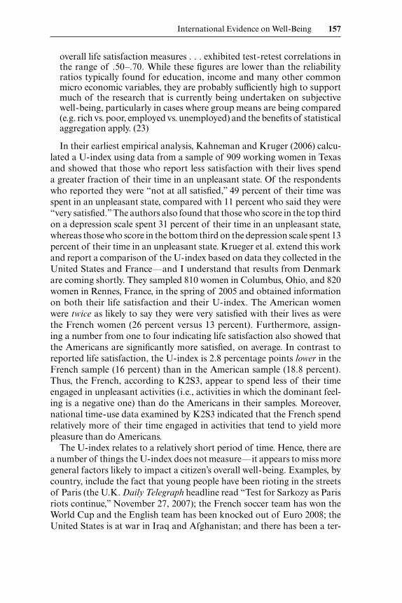
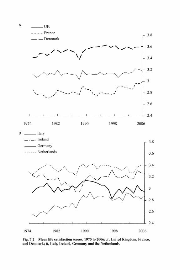
For the United States there seems to be relatively little evidence that despite rising affluence, happiness or life satisfaction have trended up much over time (Blanchfl ower and Oswald 2004a). For example, in the 2006 GSS, 13.1 percent of respondents said they were not too happy, 56.1 percent said they were pretty happy, and 30.8 percent said they were very happy. In 1972, the fi rst year happiness data are available, the numbers were 16.5 percent, 53.2 percent, and 30.3 percent, respectively. As can be seen from fi gure 7.1, average happiness levels for the United States are fl at, while real gross domestic product (GDP) per capita has risen. It is also apparent from table 1.18 of K2S3 that their U- index based on time in various activities each year is also fl at over time, as seen in table 7.1. The picture is more mixed among European countries. For example, in fi gure 7.2, panels A and B, there is some sign of a strong long- run upward trend in Italy, and to a lesser extent in Denmark and France, while the data are relatively fl at in the Netherlands, Germany, the United Kingdom, and Ireland. In contrast,


Belgium and Portugal have signifi cant downward trends (results not re-ported). Note that happiness levels are generally high in Denmark and low in Italy and France. In addition, Frey and Stutzer (2002b) have shown that the time trend in life satisfaction in Japan was fl at between 1958 and 1991, the period when GDP per capita rose by a factor of six.

There is evidence, however, of upward trends in Eastern European coun-tries, Turkey, and South American countries over the recent past. Table 7.2 reports the distribution of life satisfaction scores over the recent past for countries from Western and Eastern Europe and from Latin America. Among the seventeen Western European countries, since the turn of the century, fi ve have seen satisfaction broadly fl at (Denmark, Greece, Ireland, Spain, and the United Kingdom); fi ve have seen increases (Belgium, Finland, France, Luxembourg, and Sweden); and seven have seen declines (Austria, Germany, Italy, Japan, the Netherlands, Portugal, and the United States). In contrast, with the exception of Hungary, all of the Eastern European countries and Turkey have all seen increases, as is the case for all the Latin

Fig. 7.1 Average happiness and real GDP per capita for repeated cross- sections of Americans

Table 7.1 Happiness averages: General Social Surveys, U.S.

1965–1966

(%) 1975–1976

(%) 1985 (%)

1992–1994 (%)

2003 (%)

2005 (%)

All 20.1 19.5 19.5 20.0 19.3 19.6Men 20.9 20.4 20.1 20.2 19.6 19.9Women 19.4 18.7 19.0 19.8 19.2 19.4

B

A

Fig. 7.2 Mean life satisfaction scores, 1975 to 2006: A, United Kingdom, France, and Denmark; B, Italy, Ireland, Germany, and the Netherlands.

Table 7.2 4- step life satisfaction: Europe, the United States, Japan, and Latin America

2001 2002 2003 2004 2005 2006

Western countriesAustria 3.18 3.13 3.08 3.05 3.04 3.08Belgium 3.06 2.96 3.04 3.18 3.16 3.19Denmark 3.60 3.61 3.57 3.59 3.62 3.61Finland 3.11 3.14 3.15 3.29 3.26 3.23France 2.94 2.88 2.85 2.95 2.96 3.00Germany 2.94 2.86 2.75 2.96 2.93 2.87Greece 2.66 2.66 2.66 2.73 2.66 2.67Ireland 3.26 3.18 3.15 3.32 3.29 3.28Italy 2.93 2.95 2.86 2.86 2.83 2.85Japan 2.71 2.61 2.59 2.74 2.58 n.a.Luxembourg 3.31 3.30 3.25 3.44 3.42 3.39Netherlands 3.42 3.31 3.28 3.33 3.41 3.36Portugal 2.71 2.63 2.49 2.49 2.48 2.44Spain 3.07 3.02 3.01 3.13 3.03 3.08Sweden 3.35 3.32 3.28 3.40 3.42 3.39U.K. 3.21 3.18 3.17 3.23 3.20 3.19U.S. 3.35 3.33 3.37 3.42 n.a. n.a.

East Europe � TurkeyBulgaria 2.08 2.04 2.05 2.06 2.04 1.99Czech Republic 2.84 2.84 2.73 2.82 2.93 2.92Estonia 2.44 2.52 2.48 2.74 2.72 2.74Hungary 2.54 2.63 2.53 2.44 2.53 2.50Latvia 2.54 2.47 2.54 2.52 2.62 2.62Lithuania 2.29 2.46 2.52 2.55 2.56 2.62Poland 2.65 2.71 2.67 2.81 2.77 2.80Romania 2.12 2.20 2.10 2.32 2.35 2.33Slovakia 2.48 2.54 2.47 2.59 2.64 2.70Slovenia 3.04 3.03 3.04 3.17 3.10 3.09Turkey 2.26 2.43 2.71 2.87 2.90 2.84

1997 2000 2001 2003 2004 2005

Latin AmericaArgentina 2.14 2.21 2.82 2.91 2.92 2.94Bolivia 1.97 1.89 2.54 2.77 2.42 2.57Brazil 2.34 2.61 2.71 2.71 2.67 2.73Colombia 2.50 2.40 3.06 3.16 3.14 3.17Costa Rica 2.82 2.65 3.34 3.46 3.29 3.34Chile 2.32 2.84 2.82 2.92 2.80 2.85Ecuador 2.06 1.86 2.74 3.03 2.48 2.68El Salvador 2.49 2.34 2.90 3.34 2.88 2.90Guatemala 2.40 2.64 3.01 3.15 3.03 3.13Honduras 2.41 2.62 3.28 3.21 3.17 2.98Mexico 2.61 2.71 2.95 3.13 2.96 3.06Nicaragua 2.67 2.16 2.96 3.18 2.77 2.94Panama 2.38 2.78 2.64 3.17 3.13 3.21


Table 7.2 (continued)

1997 2000 2001 2003 2004 2005

Paraguay 2.16 2.14 2.93 3.26 2.84 2.95Peru 1.70 1.72 2.48 2.74 2.49 2.50Uruguay 2.40 2.36 2.91 2.88 2.73 2.90Venezuela 2.45 2.82 3.26 3.36 3.26 3.45

Source: Blanchfl ower and Shadforth (2007), plus Eurobarometers, Latinobarometers, and the World Database of Happiness.

American countries from 1997.1 There is also some consistent evidence that the well- being of the young (less than thirty years old) has risen over time in both the United States and Europe (Blanchfl ower and Oswald 2000). The rise is mostly among the unmarried. We found that this upward trend is not explained by changing education or work, falling discrimination, or the rise of youth- oriented consumer goods.

There is some evidence of convergence over time in the happiness of men and women in the United States, as women have become less happy (Blanchfl ower and Oswald 2004a). Stevenson and Wolfers (2007) fi nd that the relative decline in women’s well- being holds for both working and stay- at- home moms, for those married and divorced, for the old and the young, and across the education distribution. The relative decline in well- being holds across various data sets, regardless of whether one asks about hap-piness or life satisfaction. Stevenson and Wolfers fi nd that the exception to this is that African American women have become happier over this period, as have African American men, and there has been little consistent change in the gender happiness gap among African Americans over this period. As with U.S. women, Stevenson and Wolfers fi nd that the well- being of Euro-pean women has declined relative to men. However, while U.S. women also experienced an absolute decline in well- being, the subjective well- being of European men and women has risen over time.

There is also intriguing new evidence that high frequency happiness data yields information about preferences. Kimball et al. (2006), for example, showed that happiness dipped signifi cantly in the fi rst week of September 2005, after the seriousness of the damage caused by Hurricane Katrina started to become apparent. The dip in happiness lasted two or three weeks and was especially apparent in the South Central region, closest to the dev-astated area.

1. Easterlin and Zimmermann (2008) suggest that the observed increases in happiness in East Germany have arisen following a noticeable drop in life satisfaction at the time of unifi cation (Blanchfl ower 2001), so the rise is largely a recovery to pretransition levels. In private commu-nication, Dick Easterlin has further suggested that based on his recent work, the collapse and recovery of life satisfaction is typically the case for the European transition countries.


7.2 The U- Index

The fi rst column of table 7.3 is taken from K2S3 and reports their U- index, which should be thought of as the inverse of a subjective well- being or happiness index. The higher the U- index, the more unhappy the person is. There is little difference by gender, and blacks are especially unhappy, as are the poor and the least educated. Unhappiness declines with age and is particularly low for the married and high for the widowed. How do these fi ndings compare with those found using happiness and life satisfaction data? Column (2) presents the proportion of people in the United States from the GSS of 2000 to 2006 who say they are very happy (on a one to three scale), while column (3) presents the proportion of Europeans from the 2000 to 2006 Eurobarometers who say they are very satisfi ed (on a one to four scale). The fi nal column reports the proportion of Latin Americans from the 2005 and 2006 Latinobarometers who say they are very satisfi ed (on a one to four scale).2 Here a larger proportion means happier people, which is the inverse of the U- index. Interestingly, the results are very similar in all four columns. Happiness is higher for the more educated, for married people, for those with higher incomes, and for whites.

Happiness does rise with age in the United States, but once controls are included, happiness is U- shaped in age (Blanchfl ower and Oswald 2008b). It is U- shaped in age in both the European and Latin American countries, even in the raw data and even when controls are included (Blanchfl ower and Oswald 2007b).3 This result is confi rmed by K2S3 in their table 1.19, where unhappiness seems to follow an inverted U- shape.4 We explore this

2. The countries covered in these Eurobarometers are Austria, Belgium, Bulgaria, Croatia, Cyprus, Czech Republic, Denmark, Estonia, Finland, France, Germany, Greece, Hungary, Ireland, Italy, Latvia, Lithuania, Luxembourg, Malta, the Netherlands, Norway, Poland, Por-tugal, Romania, Slovakia, Slovenia, Spain, Sweden, Turkey, and the United Kingdom. The Latinobarometer covers Argentina, Bolivia, Brazil, Chile, Colombia, Costa Rica, Dominican Republic, Ecuador, El Salvador, Guatemala, Honduras, Mexico, Nicaragua, Panama, Para-guay, Peru, Uruguay, and Venezuela.

3. As Clark (2007) notes, this fi nding is repeated in happiness equations in Blanchfl ower and Oswald (2004a); Clark (2005); Clark and Oswald (1994); Di Tella, MacCulloch, and Os-wald (2001); Frey and Stutzer (2002a); Frijters, Haisken- DeNew, and Shields (2004); Gerdtham and Johannesson (2001); Graham (2005); Helliwell (2003); Kingdon and Knight (2007); Lelkes (2007); Oswald (1997); Powdthavee (2005); Propper et al. (2005); Sanfey and Teksoz (2007); Senik (2004); Shields and Wheatley Price (2005); Theodossiou (1998); Uppal (2006); Van Praag and Ferrer- i- Carbonell (2004); and Winkelmann and Winkelmann (1998).

4. Blanchfl ower and Oswald (2008b) fi nd that a robust U- shape in age in happiness and life satisfaction is found in seventy- two countries—Albania, Argentina, Australia, Azerbaijan, Belarus, Belgium, Bosnia, Brazil, Brunei, Bulgaria, Cambodia, Canada, Chile, China, Colom-bia, Costa Rica, Croatia, Czech Republic, Denmark, Dominican Republic, Ecuador, El Salva-dor, Estonia, Finland, France, Germany, Greece, Honduras, Hungary, Iceland, Iraq, Ireland, Israel, Italy, Japan, Kyrgyzstan, Laos, Latvia, Lithuania, Luxembourg, Macedonia, Malta, Mexico, Myanmar, the Netherlands, Nicaragua, Nigeria, Norway, Paraguay, Peru, Philippines, Poland, Portugal, Puerto Rico, Romania, Russia, Serbia, Singapore, Slovakia, South Africa, South Korea, Spain, Sweden, Switzerland, Tanzania, Turkey, Ukraine, the United Kingdom, the United States, Uruguay, Uzbekistan, and Zimbabwe.

Table 7.3 U- index, happiness, and life satisfaction for various demographic groups

U- index (%) GSS (%) EB (%) LB (%)

Sex Men 17.6 30.9 27.0 30.5 Women 19.6 31.3 26.8 30.1Race/ethnicity White 17.5 32.7 Black 23.8 26.6 Hispanic 21.9 24.8Household income �$30,000 22.5 31.8 $30,000–$50,000 18.6 23.6 $50,000–$100,000 ($110k) 18.6 38.2 �$100,000 15.7 46.8Education �High school/�16 years 20.5 28.9 19.3 28.0 High school/16–19 years 21.3 31.2 25.1 31.6 Some college/20� years 19.6 31.7 34.8 32.4 College/still studying 15.6 37.2 32.5 Masters 16.6 36.6 Doctorate 11.3 36.4Men 15–24 18.8 23.4 28.0 34.1 25–44 17.1 29.2 25.7 30.8 45–64 18.7 33.0 25.9 27.6 65� 15.6 39.8 30.5 28.0 Married 17.4 39.0 29.3 33.6 Divorced/separated 24.3 17.5 18.6 27.1 Widowed 20.2 22.1 21.6 Never married 16.9 20.3 23.3 29.1Women 15–24 18.9 29.5 28.9 33.7 25–44 20.5 32.0 28.1 30.5 45–64 20.9 33.5 25.4 26.6 65� 16.1 33.6 24.6 28.7 Married 17.4 41.6 29.4 32.9 Divorced/separated 24.5 20.3 18.7 29.0 Widowed 22.3 25.0 20.7 Never married 23.2 24.1 24.9 29.8

Source: GSS pooled 2000, 2002, 2004, 2006—percent “very happy.” Eurobarometers for EU15 from 2000 to 2006—% “very satisfi ed” (Austria, Belgium, Denmark, Finland, France, Germany, Greece, Ireland, Italy, Luxembourg, the Netherlands, Portugal, Spain, Sweden, and United Kingdom). Krueger et al. (2007)—table 5.1 using Princeton Affect and Time Survey data. Latinobarometer 2005—% “very satisfi ed” (Argentina, Bolivia, Brazil, Colombia, Costa Rica, Chile, Dominican Republic, Ecuador, El Salvador, Guatemala, Honduras, Mexico, Ni-caragua, Panama, Paraguay, Peru, Uruguay, and Venezuela). Education categories for the LB are “�9 years schooling,” “10–12 years schooling,” and “�12 years schooling.”Note: U- index is proportion of time that rating of “sad,” “stressed,” or “pain” exceeds “happy.”EB � Eurobarometer, LB � Latinobarometer.


U- shape in age in more detail next. The patterns across individuals are essen-tially the same then, for subjective well- being (SWB) and NTA in the United States, Latin America, and Europe. It turns out that the happiness derived from sex in both SWB studies and in U- index studies is especially high. Blanchfl ower and Oswald (2004b) found that sexual activity enters strongly positively into happiness equations.5 Indeed, in Kahneman and Krueger (2006) and Kahneman et al. (2004b), “intimate relations” has the lowest rating (i.e., gives the most happiness), while “commuting” has the highest. Though somewhat surprisingly, in K2S3, “walking” gave more happiness than “making love” among U.S. women, although the reverse was the case among French women (table 1.22)!

In section 1.8 of their chapter, K2S3 do some international comparisons of SWB in two representative cities—one in France and the other in the United States—and ask whether the standard measure of life satisfaction and the NTA yield the same conclusion concerning relative well- being. Specifi cally, they designed a survey to compare overall life satisfaction, time use, and recalled affective experience during episodes of the day for random samples of women in Rennes, France, and Columbus, Ohio. The authors argued that these cities were selected because they represented “middle America” and “middle France.” Krueger et al. also presented results using time allocation derived from national samples in the United States and France to extend their analysis beyond these two cities. The city sample consisted of 810 women in Columbus, Ohio, and 820 women in Rennes, France. Respondents were invited to participate based on random- digit dialing in the spring of 2005 and were paid approximately $75 for their participation. The age range spanned from eighteen years old to sixty- eight years old, and all participants spoke their country’s dominant lan-guage at home. The Columbus sample was older (median age of forty- four years old versus thirty- nine years old), more likely to be employed (75 per-cent versus 67 percent), and better educated (average of 15.2 years of school versus fourteen years) than the Rennes sample, but the Rennes sample was more likely to currently be enrolled in school (16 percent versus 10 per-cent). The life satisfaction question was taken from the World Values Sur-vey (WVS).

The distribution of reported life satisfaction in Columbus, Ohio, and Rennes, France, for women found by K2S3 is presented in the fi rst two columns of part A of table 7.4 using the 4- step life satisfaction scale. Life satisfaction is based on the question, “Taking all things together, how satis-fi ed are you with your life as a whole these days—not at all satisfi ed, not

5. Blanchfl ower and Oswald (2004b) found that higher income does not buy more sex or more sexual partners. Married people have more sex than those who are single, divorced, widowed, or separated. The happiness- maximizing number of sexual partners in the previous year is cal-culated to be one. Highly educated females tend to have fewer sexual partners. Homosexuality has no statistically signifi cant effect on happiness.


very satisfi ed, fairly satisfi ed, or very satisfi ed?” Krueger et al. found that American women reported higher levels of life satisfaction than the French, regardless of whether the proportion who said they were “very satisfi ed” or the overall score was used. Yet they also found that on average, the French spent their days in a more positive mood. Moreover, the national time- use data they used also indicated that the French spend relatively more time engaged in activities that tend to yield more pleasure than do Americans. Their results, they argue, “suggest that considerable caution is required in comparing standard life satisfaction data across populations with different cultures.” In particular, the Americans seem to be more emphatic when

Table 7.4 Life satisfaction and country characteristics: France, Denmark, the United Kingdom, and the United States

K2S3, 2006Women

Eurobarometer, 2000–2006Women

U.S. France France Denmark U.K.

A. 4- step life satisfactionNot at all satisfi ed 1.6 1.1 4.5 0.6 2.2Not very satisfi ed 21.4 16.1 15.1 2.7 8.4Satisfi ed 51.0 70.0 64.5 31.7 56.6Very satisfi ed 26.1 12.9 15.9 65.0 32.9Score 3.00 2.94 2.92 3.62 3.21N 810 816 7,074 6,700 9,457

France Denmark U.K. U.S.

B. 10- step life satisfaction for women: WVS1981–1984 6.75 8.27 7.55 7.731989–1993 6.82 8.07 7.65 7.651999–2004 6.97 8.23 7.68 7.65

C. 4- step life satisfaction for men and women combined: World Database of Happiness2001 2.90 3.59 3.17 3.352002 2.89 3.59 3.14 3.332003 2.86 3.56 3.16 3.412004 2.96 3.60 3.22 3.42

D. MacrodataGDP/capita (PPP U.S.$, 2004) $29,300 $31,914 $30,821 $39,676Gini coefficient 32.7 24.7 36.0 40.8Unemployment rate 8.6% 3.3% 5.4% 4.7%Long- term unemployment 44.8% 20.7% 27.5% 10.7%Youth unemployment 23.9% 7.6% 13.9% 10.5%

Source: http://hdrstats.undp.org/indicators/.Notes: Score is obtained by calculating a weighted average of responses, where 1 � “not at all satisfi ed,” 2 � “not very satisfi ed,” 3 � “satisfi ed,” and 4 � “very satisfi ed.” “Youth unemploy-ment” and “long- term unemployment” are both for males. “Youth unemployment” is for ages 15 to 24. “PPP” means “purchasing power parity.”


reporting their well- being. The U- index, K2S3 suggests, “apparently over-comes this inclination.”

Kahneman et al. (2004a, 430) have argued that differences in the SWB ratings of Denmark and France) in the Eurobarometers, for example, are implausibly large, and they “raise additional doubts about the validity of global reports of subjective well- being, which may be susceptible to cultural differences in the norms that govern self descriptions.” For example, in the Eurobarometers from 2000 to 2006, the average distributions for life satis-faction for these two countries are as seen in table 7.5. Such differences are consistently repeated in multiple data sets, regardless of whether happiness or life satisfaction is used. It is clearly problematic to compare one coun-try’s happiness answers to those of another country. Nations have different languages and cultures, and in principle, that may cause biases—perhaps large ones—in happiness surveys. At this point in research on subjective well- being, the size of any bias is not known, and there is no accepted way to correct the data, although the literature has made some progress in explor-ing this issue (for instance, by looking inside a nation like Switzerland at subgroups with different languages). In the long run, research into ways to difference out country fi xed effects will no doubt be done, and the work of K2S3 in this regard is obviously important. For example, the strong well- being performance in some happiness surveys of countries such as Mex-ico and Brazil in the 2002 ISSP (Blanchfl ower and Oswald 2005) may or may not ultimately be viewed as completely accurate. In Blanchfl ower and Oswald (2005), one check was done by comparing happiness in the English- speaking nations of Great Britain, Ireland, New Zealand, Northern Ire-land, and the United States. The main attraction is that this automatically avoids translation problems. Moreover, this smaller group of nations has the advantage that they are likely to be more similar in culture and philo-sophical outlook, and that in turn may reduce other forms of bias in people’s answers. However, it does appear that there is considerable stability in cross- country rankings of life satisfaction in English- speaking countries (Blanch-fl ower and Oswald 2005, 2006; Leigh and Wolfers 2006).

7.3 Econometric Evidence on Life Satisfaction and Happiness

As I will show in more detail next, there is also a great deal of stability in the rankings of European countries across a number of surveys, includ-

Table 7.5 Life satisfaction averages: 2000–2006 Eurobarometers

Not at all

satisfi ed (%) Not very

satisfi ed (%) Fairly

satisfi ed (%) Very

satisfi ed (%) N

France 4 15 65 16 13,554Denmark 1 3 33 63 13,718


ing the Eurobarometers (1973 to 2006), the EQLS (2003), and the Euro-pean Social Survey (2002). Further, it seems that there is evidence from the WVS and the ISSP (2002) supporting a happiness ranking where the United States is ranked above France, as implied in K2S3’s life satisfaction data, rather than below it, as implied by their U- index. In fact, I am unable to fi nd any data fi le where the ranking reverses, as occurs with the U- index. The evidence is essentially the same, both when we look at happiness, life satisfaction, health, or family life, and conversely, when we look at a variety of measures of unhappiness including high blood pressure, stress, lack of sleep, pain, and being “down and depressed.”

Where feasible I present data comparing the United States and France, but there are only a few data fi les that include both countries, so we make use of data from a number of European data fi les that allow a direct compari-son with Denmark—which will be included in K2S3’s analysis shortly—plus the United Kingdom, which is of particular interest to this author. In almost all of what follows, the United Kingdom ranks above France: Den-mark is mostly at the top of the happiness rankings in Europe, especially when life satisfaction is used. If we refer to fi gure 7.2, panels A and B, which are based on Eurobarometer data, Denmark ranks above the United King-dom, which itself ranks above France, in every year of data we have avail-able. Indeed, based simply on life satisfaction averages, France usually ranks below the large majority of the EU- 15 (the European Union comprised of Austria, Belgium, Denmark, Finland, France, Germany, Greece, Ire-land, Italy, Luxembourg, the Netherlands, Portugal, Spain, Sweden, and the United Kingdom). For example, in the raw data from the latest Euro-barometer available, number 65.2 for March through May 2006, France ranked fourteenth out of thirty countries.6 Controlling for a variety of characteristics over a long run of thirty years, France ranked seventeenth out of thirty.7

Columns (3) through (5) of part A of table 7.4 report results using the most recent subset of the data from the Eurobarometers for 2000 to 2006, which shows that France ranks third behind Denmark and the United

6. Average life satisfaction scores were Denmark (3.61), Luxembourg (3.39), Sweden (3.39), the Netherlands (3.36), Ireland (3.28), Finland (3.23), Belgium (3.19), the United Kingdom (3.19), Cyprus (3.12), Slovenia (3.10), Austria (3.08), Spain (3.08), Turkish Cyprus (3.02), France (3.00), Malta (2.98), West Germany (2.95), Czech Republic (2.89), Italy (2.86), Turkey (2.85), Poland (2.79), Croatia (2.78), East Germany (2.72), Estonia (2.72), Greece (2.67), Slo-vakia (2.66), Lithuania (2.58), Latvia (2.56), Hungary (2.47), Portugal (2.44), Romania (2.31), and Bulgaria (1.97).

7. When an ordered logit is run using these Eurobarometer data from 1973 to 2006—pooled across all member countries, plus candidate countries Croatia, Norway, and Turkey, with a standard set of controls as in table 8, column (5)—the rankings are as follows, with rank in parentheses: Denmark (1), the Netherlands (2), Norway (3), Sweden (4), Luxembourg (5), Ire-land (6), the United Kingdom (7), Finland (8), Belgium (9), Austria (10), Cyprus (11), Slovenia (12), Malta (13), Spain (14), Germany (15), Turkey (16), France (17), Czech Republic (18), Italy (19), Croatia (20), Poland (21), Portugal (22), Estonia (23), Greece (24), Slovakia (25), Latvia (26), Lithuania (27), Hungary (28), Romania (29), and Bulgaria (30).


Kingdom. Part B of table 7.4 presents data on women using the WVS on a 10- point life satisfaction scale and replicates that ranking. Part C of the table uses data for men and women combined from the World Database of Happiness, which includes all four countries. Once again France ranks at the bottom, with Denmark second, the United Kingdom third, and the United States at the top.

In the fi nal part of table 7.4 I present some macroeconomic data on GDP per capita, the Gini coefficient, and the most recent unemployment rate (Office of National Statistics 2007). In comparison with France, the United States has (a) a lower unemployment rate, (b) a higher GDP per capita, and (c) a higher Gini coefficient. France has especially high rates of long- term unemployment and youth unemployment. Denmark has an especially low unemployment rate and low Gini coefficient. Despite the well- known difficulty of making suicide rates comparable across countries, it appears that the rates in France for both men and women are well above those for the United States. This is illustrated in table 7.6. This ranking is more con-sistent with SWB data rankings than it is with rankings based on NTA.

Table 7.6 Suicide rates (per 100,000)

United States

1950 1955 1960 1965 1970 1975 1980 1985 1990 1995 2000 2002

Total 7.6 10.2 10.6 11.1 11.5 12.7 11.8 12.3 12.4 11.9 10.4 11.0Male 17.7 15.9 16.4 16.7 16.7 18.9 18.6 19.9 20.4 19.8 17.1 17.9Female 2.5 4.5 4.9 6.1 6.5 6.8 5.4 5.1 4.8 4.4 4.0 4.2

France

1950 1955 1960 1965 1970 1975 1980 1985 1990 1995 2000 2003


Denmark

1950 1955 1960 1965 1970 1975 1980 1985 1990 1995 2000 2001


United Kingdom

1950 1955 1960 1965 1970 1975 1980 1985 1990 1995 1999 2004


Source: http://www.who.int/mental_health/prevention/suicide/country_reports/en/index.html.


Happiness from a further source, the ISSP, which also contains data from the two countries, is supportive of the fact that happiness in the United States is higher than it is in France. Data on the two countries are available in the 1998, 2001, and 2002 sweeps. In the fi rst two sweeps, happiness data is available on a 4- point scale in response to the question, “How happy are you with your life in general—not at all happy, not very happy, fairly happy, or very happy?” Responses are found in table 7.7. The overall score for the French increased between 1998 and 2001. In the 2002 ISSP, responses were provided on a 7- point scale, and the U.S. score was once again considerably higher than the French for both men and women. As can be seen in table 7.8, the average score across respondents in the United States was higher for both men and women; however, the proportion who were unhappy—completely, very, or fairly—was higher. For men in the United States, 4.3 percent in this category were unhappy, compared with 3.1 percent in France,

Table 7.7 Happiness: 1998 and 2000 ISSP

Not at all (%) Not very (%) Fairly (%) Very (%) Score (%) N

2001 U.S. 1 7 51 41 3.3 1,1291998 U.S. 2 9 52 37 3.2 1,2722001 France 1 9 62 27 3.2 1,3301998 France 3 20 64 13 2.9 1,082

Table 7.8 Happiness: 2002 ISSP

Female Male All

United StatesCompletely unhappy 0.2 0.0 0.1Very unhappy 1.5 1.2 1.4Fairly unhappy 2.5 3.1 2.8Neither 5.4 6.8 6.0Fairly happy 31.9 36.3 33.7Very happy 45.7 41.6 44.0Completely happy 13.0 11.1 12.2Score 5.56 5.47 5.52N 672 488 1,160

FranceCompletely unhappy 0.1 0.2 0.1Very unhappy 0.3 0.5 0.3Fairly unhappy 3.2 2.4 3.0Neither 13.4 10.9 12.6Fairly happy 48.8 49.1 48.9Very happy 23.6 25.0 24.1Completely happy 10.7 12.0 11.1Score 5.24 5.31 5.26

N 1,216 617 1,833


while for women, the numbers were 4.2 percent and 3.6 percent, respectively. We now turn to the econometric evidence where we are able to hold constant a number of factors including labor market and marital status, age, gender, and schooling. The rankings remain essentially unchanged.

7.3.1 Econometric Evidence on the Microdeterminants of Happiness

Rank orderings of the United States and France are consistent, whether we examine happiness, life satisfaction, or other variables relating to the fam-ily, no matter what data fi le or year we examine. Tables 7.9 and 7.10 explore differences in happiness between the United States and France using the ISSP 1998, 2001, and 2002 data previously described.8 In all three years of data, the United States ranks above France, although there is some variation in the rankings across other countries. For example, the United Kingdom is above the United States in 1998 and 2001, but below it in 2002; it is also above Denmark in all three years, while Denmark is below France in 2001. In most other data fi les we examine, Denmark ranks at the top in Europe, especially on life satisfaction. Columns (3) and (4) provide estimates of ordered logits estimating how satisfi ed an individual is with their family life. The idea here is to ensure the rankings are not driven by different interpretations of the word “happy,” although they are still potentially impacted by the reticence of the French to be emphatic when reporting their well- being. Rankings are similar to those based on happiness, with Americans more satisfi ed than the French. It does seem, however, that people in the United States value time with their families very highly. Interestingly, when individuals in the ISSP are asked whether they wished they could spend more time with their families, more than half of respondents reported they would like to spend “much more time,” compared with a third in France and the United Kingdom and a fi fth in Denmark (table 7.11).

It is appropriate to explore further the ranking by country using the SWB measures from other data fi les to see if the rankings are consistent. This is what is done in tables 7.12 through 7.14, and it turns out they are. Table 7.12 uses data from eighty- two countries from the four sweeps of the WVS of 1981 to 2004 on both life satisfaction and happiness. Ordered logits are estimated in columns (1) and (2) with the dependent variable—life satisfac-tion—and responses are scored on a scale of one to ten, where one is least satisfi ed and ten is most satisfi ed. The sample size is just over one- quarter million observations—only three country dummies are included, with the remaining country dummies all excluded for simplicity. The fi rst column only includes nineteen year dummies and country dummies for France, Den-mark, the United Kingdom, and the United States, with all other countries

8. The exact question asked is Q.17: “If you were to consider your life in general, how happy or unhappy would you say you are, on the whole?”—1 � completely happy, 2 � very happy, 3 � fairly happy, 4 � neither happy nor unhappy, 5 � fairly unhappy, 6 � very unhappy, and 7 � completely unhappy.

Table 7.9 Happiness equations: 1998 and 2001 ISSP

1998 2001

(1) (2) (3) (4)

Denmark .6415 (7.32) .6554 (7.39) .2451 (2.86) .2664 (3.05)France –.2635 (3.00) –.3977 (4.49) .2699 (3.22) .3043 (3.59)U.K. .8500 (10.55) .8920 (10.97) .5855 (7.64) .7097 (9.16)Australia .6791 (8.06) .6196 (7.17) .2599 (3.12) .2942 (3.41)Austria .3595 (4.02) .3139 (3.48) .3252 (3.63) .4093 (4.52)Brazil 1.2895 (16.34) 1.4270 (17.10)Bulgaria –1.4468 (16.31) –1.4724 (16.39)Canada .2404 (2.63) .0987 (1.06) .5587 (6.42) .5751 (6.45)Chile –.5378 (6.32) –.6176 (7.20) .4707 (5.64) .5407 (6.39)Cyprus –.2714 (2.95) –.4533 (4.88) –.9342 (10.26) –1.0880 (11.83)Czech Republic –.3740 (4.41) –.4048 (4.73) –.5579 (6.47) –.5132 (5.87)East Germany –.6886 (7.70) –.5614 (6.25) –.3648 (3.18) –.2484 (2.16)Finland –.3058 (3.65) –.3262 (3.79)Hungary –1.5248 (17.34) –1.4973 (16.84) –.7982 (9.71) –.6713 (8.06)Ireland 1.2023 (13.53) 1.2171 (13.51) .0850 (1.02)Israel –.1655 (1.88) –.3189 (3.59) –.3637 (4.10) –.4534 (5.06)Italy –.3475 (3.88) –.4527 (5.03) –.6034 (6.64) –.8020 (8.56)Japan .0343 (0.41) –.1062 (1.26) .1487 (1.76) .0985 (1.15)Latvia –1.4895 (17.63) –1.5736 (18.41) –1.4145 (15.85) –1.3995 (15.50)Netherlands .7338 (9.48) .7252 (9.30)New Zealand .7760 (8.70) .7544 (8.31) .7155 (8.27) .7782 (8.80)Norway .2935 (3.58) .2269 (2.73) .0872 (1.06) .0850 (1.02)Philippines .2444 (2.79) –.0038 (0.04) .1119 (1.28) .0772 (0.87)Poland –.0188 (0.21) –.0332 (0.38) –.5691 (6.61) –.5061 (5.83)Portugal –.9207 (10.49) –1.0417 (11.82)Russia –1.3633 (16.72) –1.4252 (17.16) –2.5134 (32.28) –2.5377 (32.23)Slovakia –.9608 (11.40) –1.1135 (13.04)Slovenia –.7625 (8.47) –.9077 (9.99) –.5625 (6.31) –.6460 (7.17)South Africa –.1925 (2.46) –.0077 (0.10)Spain .1531 (2.03) .0883 (1.17) –.2714 (3.20) –.2837 (3.31)Sweden .2767 (3.18) .1541 (1.75)Switzerland .5572 (6.49) .5453 (6.28) .7205 (8.12) .7698 (8.52)U.S. .8065 (9.49) .8325 (9.72) .7800 (8.98) .9193 (10.45)Age –.0738 (17.72) –.0630 (15.17)Age2 .0006 (14.76) .0006 (13.29)Male –.0960 (4.23) –.0180 (0.80)Personal controls No Yes No Yes

Cut1 –3.6133 –5.4182 –3.5164 –4.9288Cut2 –1.5153 –3.2445 –1.7275 –3.0885Cut3 1.4123 –.2039 1.1509 –.1180

N 37,875 37,521 35,950 35,219Pseudo R2 .0607 .0857 .0765 .0964

Source: 1998 and 2001 ISSP.Notes: Personal controls are marital status and labor market status dummies. Excluded country: West Germany. “If you were to consider your life in general, how happy would you say you are, on the whole—not at all happy, not very happy, fairly happy, or very happy?”

Table 7.10 Happiness and role of the family: 2002 ISSP

Happiness Family

(1) (2) (3) (4)

Denmark –.1159 (1.53) .3825 (4.95)France –.3039 (4.40) –.4605 (6.41)U.K. .3613 (5.65) .3082 (4.65)U.S. .6701 (8.30) .4169 (5.45) .7448 (9.36) .3612 (4.56)Age –.1084 (7.26) –.0705 (19.55) –.1032 (7.06) –.0675 (18.53)Age2 .0011 (7.29) .0006 (17.50) .0010 (6.91) .0006 (17.03)Male –.0261 (0.35) .0507 (2.68) –.0758 (1.02) .1118 (5.87)No formal education .5095 (1.36) .0208 (0.49) –.1011 (0.28) .0432 (1.05)Above lowest formal .2813 (2.02) .1833 (4.32) –.0020 (0.01) .1848 (4.43)Higher secondary .5644 (3.97) .2459 (5.81) .0738 (0.21) .2191 (5.28)Above secondary .5243 (3.75) .2957 (6.52) .0035 (0.01) .2207 (4.93)University degree .8726 (6.44) .4026 (8.92) .1145 (0.33) .2392 (5.37)Married .9005 (9.00) .7009 (26.23) 1.1943 (11.93) .8491 (31.05)Widowed .0561 (0.30) –.2500 (5.54) .4089 (2.24) –.1107 (2.41)Divorced –.0866 (0.63) –.2372 (5.46) .0597 (0.44) –.3134 (6.96)Separated –.4838 (2.16) –.3636 (5.53) –.3306 (1.53) –.5151 (7.85)Public sector .0291 (0.29) .0392 (1.41) –.0114 (0.12) .0050 (0.18)Self- employed .0980 (0.65) .1061 (3.11) .1601 (1.08) .0911 (2.69)Unpaid family worker –.7075 (0.91) .0398 (0.33) .2213 (0.25) –.0415 (0.35)Unemployed –.2388 (1.24) –.5482 (12.92) –.2223 (1.17) –.3923 (9.24)Student .0559 (0.28) .1459 (3.13) .0872 (0.42) .1028 (2.16)Retired –.0991 (0.67) –.0496 (1.34) –.0267 (0.18) –.0625 (1.68)Housewife –.0016 (0.01) .0363 (1.01) –.0246 (0.18) .0038 (0.11)Disabled –.5181 (1.04) –.4661 (6.60) –.5115 (1.11) –.3052 (4.29)Other labor market –.3538 (1.35) –.2712 (4.43) –.5177 (1.94) –.2909 (4.77)Austria .4277 (6.34) .5102 (7.24)Brazil .4371 (6.13) –.3380 (4.64)Bulgaria –1.6116 (20.47) –1.3513 (16.66)Chile .4715 (6.41) .5708 (7.70)Cyprus –.0927 (1.16) –.1089 (1.38)Czech Republic –.7562 (10.08) –.8577 (11.23)East Germany –.6619 (6.41) –.1039 (0.98)Estonia –.2654 (4.06) –.2251 (3.37)Finland –.3428 (4.44) –.3863 (4.86)Flanders –.3712 (4.98) –.2767 (3.62)Hungary –.5945 (7.41) –.2962 (3.59)Ireland –.0298 (0.41) .4107 (5.34)Israel –.2329 (3.00) .1679 (2.13)Japan .2953 (3.70) –.2731 (3.40)Latvia –1.1807 (14.87) –1.1642 (14.13)Mexico .5591 (7.34) .8134 (10.61)Netherlands –.2270 (3.06) –.1761 (2.30)New Zealand .2682 (3.30) .1114 (1.34)Norway –.1811 (2.48) –.0272 (0.37)Philippines .1092 (1.37) .0601 (0.74)Poland –.7878 (10.48) –.3929 (5.11)Portugal –.3820 (4.82) –.2205 (2.75)



Happiness Family

(1) (2) (3) (4)

Russia –1.0997 (15.45) –1.0436 (14.00)Slovakia –.9487 (12.21) –.8533 (10.61)Slovenia –.4791 (6.15) –.1456 (1.81)Sweden –.2411 (3.06) .0495 (0.60)Switzerland .3338 (4.28) .2935 (3.68)Taiwan –.3847 (5.59) –.4845 (6.95)West Germany –.4315 (5.36) –.0499 (0.60)

Cut1 –8.1600 –7.5073 –6.3764 –6.4968Cut2 –6.0305 –5.9530 –5.2860 –5.4063Cut3 –4.5138 –4.5258 –3.9864 –4.1993Cut4 –3.0443 –2.9599 –3.0898 –3.0322Cut5 –.7444 –.8420 –1.3159 –1.1549Cut6 1.1677 1.1391 .2919 .7428

Pseudo R2 .0460 .0456 .0444 .0442N 2,885 44,468 2,859 43,657

Notes: Excluded categories are: “lowest formal qualifi cation,” “private sector employee,” and Australia. T- statistics are in parentheses. Columns (1) and (3) are U.S. and France only. Columns (1) are (2) are responses to the question, “If you were to consider your life in general, how happy or unhappy would you say you are, on the whole?” (Respondents answered on a 7- point scale.) Column (2) refers to the fol-lowing question: “All things considered, how satisfi ed are you with your family life?” (Respondents an-swered on a 7- point scale.) Scale is “completely unhappy,” “very unhappy,” “fairly unhappy,” “neither,” “fairly happy,” “very happy,” and “completely happy.”

set as the omitted category for simplicity. Column (2) adds controls for age, gender, marital status, and labor market status. Happiness is higher among the married (Zimmermann and Easterlin 2006) and the educated and is especially low among the unemployed (Blanchfl ower and Oswald 2004a, 2004b). In both columns the country ranking remains as follows: France, the United Kingdom, the United States, and Denmark. In columns (3) and (4) the dependent variable is a 4- step happiness variable and the rankings are a little different: France, the United States, the United Kingdom, and again Denmark at the top. These results are consistent with the fi ndings of Veenhoven (2000), who examined the fi rst three waves of the WVS and found that among the three possible ways of ranking countries—based on responses of individuals on how happy they are, how satisfi ed they are, and how they would rate their lives on a scale from the worst to the best possible life—the ranking stays roughly the same.

Table 7.13 uses data from another source, the 2003 EQLS (n � 26,000), which obviously excludes the United States and follows a similar form, but this time separate results are reported on a 10- step scale for life satisfaction and happiness. Data are also available on the individual’s assessment of their overall health on a 5- point scale: poor, fair, good, very good, and excellent.

Table 7.11 Wanting to spend time with the family—ranked by percentage in 2005

1997 (%) 2005 (%)

United States 41.9 55.3Dominican Republic 55.3Mexico 43.5Philippines 50.8 38.7Canada 23.3 37.8South Africa 36.7France 34.3 33.7Israel 35.6 33.5New Zealand 23.9 28.6Australia 28.5Ireland 28.1United Kingdom 31.6 27.7East Germany 29.8 25.7Sweden 27.9 25.7Norway 25.5 24.8Slovenia 26.3 23.3West Germany 24.5 21.4Denmark 21.0 21.2Portugal 34.1 19.8Russia 23.9 19.3Hungary 19.1 18.7Switzerland 22.8 17.1Bulgaria 14.7 16.7Czech Republic 25.2 15.1Spain 7.8 15.0Finland 14.4South Korea 13.1Japan 7.5 9.1Taiwan 8.9Cyprus 25.2 7.2Bangladesh 5.1Italy 15.7Latvia 15.6Netherlands 14.6

Poland 23.4

Source: 1997 ISSP (n � 32,783) and 2005 (n � 43,440).Notes: Question asked is, “Suppose you could change the way you spend your time, spending more time on some things and less time on others. Which of the things on the following list would you like to spend more time on, which would you like to spend less time on, and which would you like to spend the same amount of time on as now?” (1 � Much more time, 2 � A bit more time, 3 � Same time as now, 4 � A bit less time, and 5 � Much less time.) Tabulated are the proportions saying “much more time” with their family.

Table 7.12 Life satisfaction and happiness: 1981–2004 World Values Survey (ordered logits)

Life satisfaction Happiness

Denmark .9958 (31.91) 1.0033 (31.47) .8450 (24.83) .8625 (24.78)France –.1073 (3.88) –.1470 (5.11) .4227 (13.64) .4426 (13.74)U.K. .5004 (22.79) .2823 (11.91) .8036 (30.05) .6773 (23.67)U.S. .5197 (23.77) .3480 (14.59) .6959 (28.04) .5800 (21.41)Age –.0377 (22.09) –.0491 (26.11)Age2 .00046 (24.75) .00050 (24.63)Male –.0765 (8.45) –.0848 (8.38)Married .1907 (14.98) .4063 (28.44)Living together .2133 (10.00) .3131 (13.04)Divorced –.3442 (14.18) –.3737 (13.82)Separated –.4235 (12.29) –.4364 (11.36)Widowed –.4123 (18.33) –.4927 (19.98)Part- time employee –.0252 (1.56) –.0064 (0.36)Self- employed .0361 (2.32) .0612 (3.50)Retired –.2202 (12.43) –.2276 (11.73)Home worker .0607 (4.21) .1494 (9.35)Student –.0158 (0.84) .0824 (3.87)Unemployed –.6850 (40.79) –.4884 (26.36)Other –.2326 (6.80) –.0245 (0.64)

Cut1 –3.4057 –4.0057 –3.6190 –4.3648Cut2 –2.8445 –3.4499 –1.4905 –2.2030Cut3 –2.2542 –2.8627 1.0105 .4280Cut4 –1.8110 –2.4062Cut5 –1.0434 –1.6032Cut6 –.5878 –1.1143Cut7 –.0103 –.4836Cut8 .8544 .4453Cut9 1.5985 1.2323Year dummies 19 19 19 19Schooling dummies 0 10 0 10

N 263,097 188,529 257,881 185,629Pseudo R2 0.0112 .0191 .0131 .0336

Notes: Excluded category is “full- time employees.” Excluded countries are: Albania, Algeria, Argentina, Armenia, Australia, Austria, Azerbaijan, Bangladesh, Belarus, Belgium, Bosnia and Herzegovina, Brazil, Bulgaria, Canada, Chile, China, Colombia, Croatia, Czech Repub-lic, Dominican Republic, Egypt, El Salvador, Estonia, Finland, Georgia, Germany, Greece, Hungary, Iceland, India, Indonesia, Iran, Iraq, Ireland, Israel, Italy, Japan, Jordan, Korea, Kyrgyzstan, Latvia, Lithuania, Luxembourg, Macedonia, Malta, Mexico, Moldova, Mo-rocco, the Netherlands, New Zealand, Nigeria, Norway, Pakistan, Peru, Philippines, Poland, Portugal, Puerto Rico, Romania, Russia, Saudi Arabia, Serbia and Montenegro, Singapore, Slovakia, Slovenia, South Africa, Spain, Sweden, Switzerland, Taiwan, Tanzania, Turkey, Uganda, Ukraine, Uruguay, Venezuela, Vietnam, and Zimbabwe.

Tab

le 7

.13

Hap

pine

ss: 2

003

Eur

opea

n Q

ualit

y of

Lif

e S

urve

y (o

rder

ed lo

gits

)

Lif

e sa

tisf

acti

on

Hap

pine

ss

Aus

tria

.409

0 (5

.10)

.427

1 (5

.27)

.428

9 (4

.49)

.142

8 (1

.79)

.156

7 (1

.93)

.236

4 (2

.47)

Bel

gium

.038

2 (0

.49)

.060

1 (0

.76)

.117

8 (1

.21)

–.15

05 (1

.94)

–.13

05 (1

.64)

.024

8 (0

.26)

Bul

gari

a–2

.536

8 (3

1.15

)–2

.440

4 (2

9.46

)–1

.544

6 (1

4.49

)–1

.969

6 (2

3.99

)–1

.789

6 (2

1.30

)–1

.017

9 (9

.45)

Cyp

rus

–.09

81 (1

.04)

–.56

91 (5

.95)

–.39

93 (3

.47)

–.02

03 (0

.22)

–.59

92 (6

.26)

–.50

23 (4

.35)

Cze

ch R

epub

lic–.

8607

(10.

67)

–.84

86 (1

0.29

)–.

4109

(3.9

9)–.

6880

(8.6

5)–.

5519

(6.7

7)–.

0797

(0.7

8)D

enm

ark

1.13

01 (1

4.11

).9

682

(11.

68)

.994

6 (1

0.42

).4

876

(6.1

7).3

591

(4.3

5).4

889

(5.1

5)E

ston

ia–1

.414

3 (1

5.42

)–1

.117

6 (1

1.94

)–.

5002

(4.5

2)–1

.042

4 (1

1.19

)–.

5971

(6.2

7)–.

0060

(0.0

5)F

inla

nd.7

337

(9.3

1).8

776

(10.

95)

.930

7 (1

0.07

).2

892

(3.7

3).5

505

(6.8

7).6

638

(7.1

7)F

ranc

e–.

5155

(6.6

7)–.

5407

(6.8

7)–.

5271

(5.6

0)–.

5903

(7.7

0)–.

6114

(7.7

7)–.

5381

(5.7

2)G

erm

any

–.05

95 (0

.75)

.017

5 (0

.22)

.168

8 (1

.77)

–.17

87 (2

.28)

–.03

40 (0

.43)

.188

6 (1

.98)

Gre

ece

–.50

31 (6

.23)

–.76

47 (9

.29)

–.49

13 (4

.61)

–.29

15 (3

.64)

–.53

31 (6

.53)

–.19

70 (1

.86)

Hun

gary

–1.3

205

(16.

37)

–1.1

253

(13.

75)

–.62

37 (6

.28)

–.76

12 (9

.36)

–.49

81 (6

.02)

–.01

20 (0

.12)

Irel

and

.305

5 (3

.83)

.119

4 (1

.48)

–.07

26 (0

.66)

.309

9 (3

.82)

.053

4 (0

.65)

–.01

87 (0

.17)

Ital

y–.

2241

(2.8

9)–.

3280

(4.1

5)–.

2784

(2.8

2)–.

3707

(4.7

9)–.

5112

(6.4

2)–.

3979

(3.9

9)L

atvi

a–1

.679

4 (2

1.04

)–1

.266

5 (1

5.48

)–.

5631

(5.5

2)–1

.494

5 (1

8.57

)–.

9902

(11.

95)

–.36

24 (3

.52)

Lit

huan

ia–1

.801

5 (2

2.55

)–1

.405

3 (1

7.23

)–.

6031

(5.9

1)–1

.417

6 (1

7.51

)–.

9009

(10.

83)

–.19

88 (1

.92)

Lux

embo

urg

.376

6 (4

.04)

.344

8 (3

.61)

.290

2 (2

.38)

.199

6 (2

.19)

.174

5 (1

.84)

.271

5 (2

.24)

Mal

ta–.

0742

(0.8

0)–.

1755

(1.8

4).0

016

(0.0

1).0

692

(0.7

5).0

152

(0.1

6).1

816

(1.4

9)N

ethe

rlan

ds.0

326

(0.4

3).1

135

(1.4

6).1

602

(1.7

0)–.

2649

(3.4

6)–.

2190

(2.7

6)–.

1452

(1.5

2)Po

land

–1.1

107

(13.

66)

–.77

42 (9

.34)

–.26

35 (2

.61)

–.93

45 (1

1.47

)–.

5367

(6.4

0)–.

0732

(0.7

2)Po

rtug

al–1

.362

1 (1

7.13

)–.

9364

(11.

45)

–.56

50 (5

.66)

–1.1

363

(14.

13)

–.63

04 (7

.62)

–.29

09 (2

.88)

Rom

ania

–1.0

805

(13.

45)

–.81

07 (9

.93)

.168

0 (1

.59)

–.69

32 (8

.76)

–.34

69 (4

.29)

.490

8 (4

.66)

Slov

akia

–1.5

512

(19.

34)

–1.5

434

(18.

76)

–1.1

304

(11.

09)

–1.3

157

(16.

74)

–1.2

635

(15.

61)

–.82

67 (8

.23)

Slov

enia

–.33

13 (3

.61)

–.25

57 (2

.75)

.052

4 (0

.48)

–.43

07 (4

.72)

–.34

49 (3

.70)

–.05

21 (0

.48)

Spai

n.0

092

(0.1

2).0

423

(0.5

2).2

027

(2.0

2)–.

0578

(0.7

2)–.

0038

(0.0

5).1

765

(1.7

4)Sw

eden

.454

5 (5

.70)

.317

8 (3

.90)

.388

6 (4

.14)

.127

5 (1

.61)

.033

0 (0

.41)

.144

6 (1

.54)

Tur

key

–1.5

390

(18.

43)

–1.4

167

(16.

39)

–.70

61 (6

.83)

–1.2

119

(14.

74)

–1.1

451

(13.

31)

–.54

24 (5

.24)

Age

–.03

72 (8

.56)

–.04

35 (8

.79)

–.03

01 (6

.89)

–.03

52 (7

.09)

Age

2.0

004

(11.

16)

.000

5 (1

1.11

).0

003

(7.7

0).0

0038

(7.7

2)M

ale

–.17

95 (7

.43)

–.19

42 (7

.11)

–.18

17 (7

.44)

–.18

01 (6

.55)

16–1

9 ye

ars

scho

olin

g.1

903

(5.7

2).1

360

(3.6

0).1

829

(5.4

4).1

370

(3.5

9)20

� y

ears

sch

oolin

g.3

223

(8.7

5).1

855

(4.4

1).2

517

(6.7

5).1

473

(3.4

7)St

ill s

tudy

ing

.211

2 (2

.21)

.056

7 (0

.52)

.335

2 (3

.51)

.164

3 (1

.50)

No

scho

olin

g–.

2564

(2.8

8)–.

2819

(2.8

0)–.

2349

(2.6

2)–.

2533

(2.5

1)Se

lf- e

mpl

oyed

.151

6 (1

.43)

.170

0 (1

.39)

.021

8 (0

.20)

–.04

19 (0

.33)

Man

ager

.301

2 (2

.91)

.317

7 (2

.69)

.137

7 (1

.29)

.078

7 (0

.65)

Oth

er w

hite

col

lar

.092

8 (0

.91)

.112

5 (0

.96)

–.05

82 (0

.55)

–.12

33 (1

.03)

Man

ual w

orke

r–.

0248

(0.2

5).0

583

(0.5

2)–.

1044

(1.0

2)–.

1115

(0.9

5)H

ome

wor

ker

.030

3 (0

.29)

.165

8 (1

.39)

–.00

13 (0

.01)

.068

5 (0

.56)

Une

mpl

oyed

–.78

98 (7

.40)

–.54

03 (4

.46)

–.69

51 (6

.35)

–.58

01 (4

.66)

Ret

ired

.117

6 (1

.15)

.281

9 (2

.43)

.099

5 (0

.95)

.165

7 (1

.39)

Stud

ent

.370

6 (2

.80)

.491

9 (3

.22)

.135

5 (1

.01)

.187

7 (1

.22)

Mar

ried

/livi

ng to

geth

er.4

165

(11.

5).3

121

(7.5

6).6

819

(18.

57)

.641

0 (1

5.36

)Se

para

ted/

divo

rced

–.25

13 (5

.05)

–.15

61 (2

.79)

–.28

46 (5

.66)

–.16

13 (2

.86)

Wid

owed

–.10

51 (2

.00)

–.06

21 (1

.06)

–.19

05 (3

.59)

–.13

74 (2

.32)

Exc

elle

nt h

ealt

h2.

3432

(41.

06)

2.23

64 (3

4.51

)2.

8968

(49.

23)

2.77

34 (4

1.60

)V

ery

good

hea

lth

1.92

04 (3

8.47

)1.

8470

(33.

09)

2.26

10 (4

4.35

)2.

1651

(38.

07)

Goo

d he

alth

1.43

78 (3

2.19

)1.

3678

(27.

81)

1.69

80 (3

7.22

)1.

6213

(32.

31)

Fai

r he

alth

.878

3 (2

0.27

).8

278

(17.

52)

1.01

35 (2

2.98

).9

574

(19.

93)

Log

hou

seho

ld in

com

e (E

uros

).3

854

(19.

33)

.298

0 (1

4.93

)

Cut

1–4

.279

6–3

.298

9–.

6592

–4.9

381

–3.7

997

–1.7

221

Cut

2–3

.728

6–2

.717

0–.

0796

–4.3

122

–3.1

498

–1.0

977

Cut

3–3

.126

2–2

.069

4.5

638

–3.6

354

–2.4

316

–.36

06C

ut4

–2.6

458

–1.5

519

1.08

99–3

.062

0–1

.813

4.2

562

Cut

5–1

.579

7–.

3838

2.28

45–2

.028

2–.

6567

1.42

75C

ut6

–1.0

325

.222

52.

8925

–1.4

683

–.01

422.

0587

Cut

7–.

2024

1.13

523.

8177

–.63

48.9

508

3.02

05C

ut8

1.07

232.

5166

5.21

06.6

150

2.37

534.

4443

Cut

91.

9941

3.48

336.

1853

1.54

503.

3891

5.46

96N

25,9

9125

,603

20,0

4725

,654

25,2

8319

,818

Pse

udo

R2

.053

5.0

885

.097

3.0

297

.082

5.0

867

Age

min

imum

47

39

50

46

Not

es: E

xclu

ded

cate

gori

es: “

sing

le,”

“ot

her

labo

r m

arke

t act

ivit

y,”

“� 1

5 ye

ars

of s

choo

ling,

” “p

oor

heal

th,”

and

the

U.K

.


Four separate controls for health status are included in column (2) for life satisfaction and in column (5) for happiness, along with a standard set of controls. Household income in Euros is also available in the data fi le, which is added in natural logarithms, in columns (3) and (6). This is the fi rst time in a cross- country data fi le on happiness that income has been available in one currency (Euros). In all cases the rankings for the three main countries of interest are France, then the United Kingdom, and fi nally highest- ranked Denmark. Eastern European countries have low levels of happiness (Blanch-fl ower 2001; Sanfey and Teksoz 2007); life satisfaction and happiness is U- shaped in age, minimizing in the mid- forties for life satisfaction and in the fi fties for happiness. Adding controls for income lowers the age minimum. Happiness rises with education and income, regardless of whether health is controlled for. Married people and those living together, as well as those in good health, are particularly happy. The unemployed are especially unhappy (Blanchfl ower and Oswald [2004a]; Carroll [2007] for Australia; Hinks and Gruen [2007] and Powdthavee [2007] for South Africa).

Money buys happiness. Interestingly, and perhaps surprisingly from an economist’s point of view, the coefficients of the other variables in the well- being equations of table 7.13 hardly alter when income is controlled for. The amount of happiness bought by extra income is not as large as some would expect. To put this differently, the noneconomic variables in hap-piness equations enter with large coefficients, relative to those of income. Following Blanchfl ower and Oswald (2004a), table 7.13, or its OLS equiva-lent (see table 7A.1), can be used to do a form of happiness calculus. The relative size of any two coefficients provides information about how one variable would have to change to maintain constant well- being in the face of an alteration in the other variable. To compensate for a major life event, such as becoming a widow or a ending a marriage, it would be necessary to provide an individual with additional income. Viewing widowhood as an exogenous event, and so a kind of natural experiment, this number may be thought of as the value of marriage. A different interpretation of this type of correlation is that happy people are more likely to stay married. It is clear that this hypothesis cannot easily be dismissed if only cross- section data are available. However, panel data on well- being suggest that simi-larly large effects are found when looking longitudinally at changes (thus differencing out person- specifi c fi xed effects). If higher income goes with more happiness and characteristics such as unemployment and being black go with less happiness, it is reasonable to wonder whether a monetary value could be put on some of the other things that are associated with disutility. Further calculation using the life satisfaction data in table 7A.1 suggests that compared with being a manual worker, to compensate for unemploy-ment would take a rise in net income of approximately €3,900 per month, which is very large, given the mean in the data of €1,392. Compared to being single, to compensate for being married or cohabiting would take


€1,770.9 Blanchfl ower and Oswald (2004a) also found large effects for the United States using the GSS data. These effects seem large and inconsistent with the claims of Kahneman et al. (2004a) that the size of the effects of circumstances on well- being are “surprisingly small.”

Table 7.14 examines data from the 2002 ESS across twenty E.U. coun-tries, plus Israel and Switzerland. Data are provided in columns (1) through

Table 7.14 Happiness, life satisfaction: 2002 European Social Survey (ordered logits)

Happiness Life satisfaction

France –.0016 (0.03) .0588 (1.24) –.5082 (10.71) –.4803 (10.03)Denmark .8828 (19.15) .7462 (16.01) 1.1833 (25.38) 1.0605 (22.55)U.K. .2033 (5.01) .1386 (3.39) –.0617 (1.55) –.1435 (3.57)Married .5126 (19.35) .4891 (18.42) .2702 (10.25) .2339 (8.86)Separated –.4287 (5.73) –.4585 (6.10) –.4754 (6.39) –.5149 (6.86)Divorced –.1309 (3.10) –.1249 (2.96) –.2130 (5.06) –.2062 (4.89)Widowed –.4401 (10.00) –.4067 (9.26) –.4055 (9.26) –.3704 (8.48)Age –.0789 (24.00) –.0634 (19.24) –.0725 (22.14) –.0564 (17.17)Age2 .0007 (23.77) .0007 (21.98) .0007 (23.77) .0007 (21.95)Male –.1421 (7.85) –.1807 (9.95) –.1550 (8.59) –.1967 (10.86)Schooling .0403 (17.03) .0224 (9.41) .0486 (20.62) .0302 (12.68)Self- employed –.0461 (1.45) –.0811 (2.54) –.0575 (1.81) –.0879 (2.76)Not employed –.2922 (13.25) –.1454 (6.53) –.3163 (14.36) –.1678 (7.55)Good health –.5999 (26.65) –.5906 (26.25)Fair health –1.2547 (45.77) –1.2830 (46.88)Bad health –2.1052 (47.99) –2.1141 (48.80)Very bad health –2.9244 (34.24) –3.0003 (36.15)

Cut1 –6.3055 –6.8664 –5.0623 –5.6024Cut2 –5.6224 –6.1758 –4.5712 –5.0994Cut3 –4.9425 –5.4806 –4.0161 –4.5278Cut4 –4.2389 –4.7518 –3.3945 –3.8793Cut5 –3.7357 –4.2258 –2.9508 –3.4121Cut6 –2.7478 –3.1797 –2.1598 –2.5686Cut7 –2.2507 –2.6484 –1.7411 –2.1194Cut8 –1.4475 –1.7908 –1.0251 –1.3520Cut9 –.2258 –.5009 .1222 –.1381Cut10 .9345 .6989 1.1579 .9339

N 40,903 40,879 40,852 40,825Pseudo R2 .0149 .0382 .0138 .0369Age minimum 56 45 52 40

Notes: Excluded categories are “very good health,” “single,” and “employee,” plus: Austria, Belgium, Czech Republic, Finland, Germany, Greece, Hungary, Ireland, Israel, Italy, Luxem-bourg, the Netherlands, Norway, Poland, Portugal, Slovenia, Spain, Sweden, and Switzer-land.

9. This is done simply by dividing the coefficient of unemployment by the coefficient of household income (i.e., 0.6847/ 0.0001715 � 3,903 Euros). The size of these effects is even higher using the happiness data (i.e., 6,420 Euros for unemployment).


(3) on happiness and life satisfaction. The rankings are very similar to those reported in table 7.13—France, then the United Kingdom, then Denmark at the top. The patterns in the data are similar to those identifi ed previously—happiness and life satisfaction is higher for the most educated, the married, the employed, and the healthy. Happiness and life satisfaction are U- shaped in age. Table 7.15 uses data from a single Eurobarometer, number 57.2, on life- satisfaction (5- step), also with and without health status dummies. There is a U- shape in age in every case. Once again, in all six cases, the rankings are France, then the United Kingdom, then highest- ranked Denmark.

Identical rankings to this are found in table 7.16, which uses over three- quarter million observations from a long time series of Eurobarometers on life satisfaction (4- step). The rank ordering is France, the United Kingdom, and Denmark for the period 1975 to 2006, as well as for all subperiods. The rankings were also the same when thirty separate equations were individu-ally run with the same controls in every year (results not reported). It is also apparent from table 7A.2 that the structure of OLS life satisfaction equations is similar across the main European countries. Interestingly, the patterns of the life satisfaction appear to be very similar to those in the hap-piness data of the United States.

Blanchfl ower and Oswald (2008b) found that psychological well- being is U- shaped through life. A difficulty with research on this issue is that there are likely to be omitted cohort effects (earlier generations may have been born in, say, particularly good or bad times). First, using data on 500,000 randomly sampled Americans and West Europeans, the paper designs a test that can control for cohort effects. Holding other factors constant, we showed that a typical individual’s happiness reaches its minimum—on both sides of the Atlantic and for both males and females—during middle age. Second, evi-dence was provided for the existence of a similar U- shape through the life course in Eastern European, Latin American, and Asian nations. Third, a U- shape in age is found in separate well- being regression equations in seventy- two developed and developing nations. Fourth, using measures that are closer to psychiatric scores, Blanchfl ower and Oswald (2008b) docu-ment a comparable well- being curve across the life cycle in two other data sets: (a) in the GHQ- N6 (General Health Questionnaire [six negative ques-tions]) mental health levels among a sample of 16,000 Europeans, and (b) in reported depression and anxiety levels among one million U.K. citizens.10 Evidence of a U- shape in age is found in all life satisfaction and happiness equations reported in this paper.11

Easterlin (2006) argues that happiness in the United States, as well as fam-ily satisfaction and job satisfaction in the United States, follow an inverse

10. Clark (2007) fi nds a similar result in the United Kingdom using data from the BHPS, even after controlling for cohort effects.

11. See tables 7.11 through 7.16 and tables 7.20 and 7.21.

Table 7.15 Life satisfaction in Europe: 2002 Eurobarometer (ordered logits)

Age –.0686 (10.97) –.0524 (8.26)Age2 .0006 (10.56) .0005 (9.03)Male –.0956 (2.79) –.1366 (3.94)ALS 16–19 .2396 (5.51) .1616 (3.67)ALS � 20 .3558 (6.95) .2533 (4.89)Still studying .4607 (4.83) .1785 (1.84)Married .3649 (6.24) .3094 (5.23)Remarried .1566 (1.12) .1712 (1.22)Living as married .0441 (0.65) .0519 (0.76)Lived together –.4266 (5.12) –.4029 (4.80)Divorced –.3551 (4.18) –.3256 (3.80)Separated –.3424 (2.73) –.2905 (2.30)Widowed –.2354 (2.75) –.2528 (2.93)Home worker –.0752 (1.12) –.2046 (3.03)Unemployed –.6153 (6.94) –.7256 (8.15)Austria .3848 (4.33) .3325 (3.70)Denmark 1.3696 (15.04) 1.3512 (14.55)East Germany –.8624 (9.94) –.7610 (8.70)Finland .4217 (4.79) .5945 (6.67)France –.7296 (8.29) –.6743 (7.60)Greece –1.6273 (18.30) –1.6692 (18.48)Ireland .4194 (4.68) .3555 (3.92)Italy –.3468 (3.93) –.2360 (2.64)Luxembourg .8863 (8.56) 1.0032 (9.57)Netherlands .7914 (8.97) .9653 (10.79)Portugal –1.6154 (18.32) –1.2698 (14.17)Spain –.2256 (2.52) –.1340 (1.48)Sweden .8549 (9.65) .9918 (11.03)U.K. .4863 (5.85) .5822 (6.93)West Germany –.2427 (2.75) –.1162 (1.31)

Good health –.6605 (16.25)Fair health –1.2178 (24.90)Bad health –1.8047 (25.42)Very bad health –2.4710 (19.85)

Cut1 –5.7366 –6.2917Cut2 –3.9623 –4.4689Cut3 –2.7567 –3.2146Cut4 .1500 –.1654

N 16,032 15,992Pseudo R2 .0911 .1197

Age minimum 57 52

Source: Eurobarometer number 57.2: Health Issues, Cross- Border Purchases, and National Identities, April to June 2002.Notes: Excluded categories are “ALS � 16,” “retired,” “excellent health,” “single,” and Bel-gium. Equations also include thirteen occupation dummies.

Tab

le 7

.16

Lif

e sa

tisf

acti

on in

Eur

ope:

197

5–20

06 E

urob

arom

eter

s (o

rder

ed lo

gits

)

1975

–198

9

1990

–199

9

2000

–200

6

1975

–200

6

1975

–200

6

Fra

nce

–1.5

161

(88.

25)

–1.4

750

(68.

29)

–1.3

120

(52.

90)

–1.4

516

(23.

07)

–1.4

453

(123

.72)

Den

mar

k.5

820

(33.

06)

.603

1 (2

6.85

).7

707

(30.

27)

.634

6 (5

2.57

).6

311

(52.

64)

U.K

.–.

4656

(28.

88)

–.55

82 (2

7.77

)–.

3871

(16.

72)

–.47

38 (4

2.96

)–.

4685

(42.

73)

Age

–.03

89 (2

4.25

)–.

0389

(20.

22)

–.03

65 (1

7.97

)–.

0379

(36.

35)

–.04

39 (5

1.02

)A

ge2

.000

47 (2

7.08

).0

0043

(21.

14)

.000

43 (1

9.86

).0

0044

(39.

84)

.000

47 (5

1.96

)M

ale

–.17

54 (1

8.19

)–.

0995

(9.3

1)–.

0843

(7.0

4)–.

1275

(20.

83)

–.09

42 (1

8.76

)M

arri

ed.3

341

(25.

83)

.306

3 (2

0.17

).5

527

(31.

33)

.363

0 (4

2.50

).3

511

(49.

32)

Liv

ing

toge

ther

.049

0 (1

.93)

.144

2 (6

.18)

.233

8 (1

0.27

).1

268

(9.4

2).1

562

(14.

23)

Div

orce

d–.

6085

(21.

31)

–.44

94 (1

6.53

)–.

3219

(11.

68)

–.47

59 (3

0.20

)–.

4055

(31.

47)

Sepa

rate

d–.

7687

(18.

55)

–.56

79 (1

2.91

)–.

4587

(10.

78)

–.60

17 (2

4.65

)–.

5303

(25.

42)

Wid

owed

–.33

19 (1

6.10

)–.

2200

(8.9

7)–.

1292

(4.5

9)–.

2566

(18.

71)

–.23

14 (2

0.58

)A

LS

16–1

9.2

485

(24.

71)

.177

8 (1

3.86

).1

819

(11.

16)

.213

7 (3

0.26

).2

234

(37.

68)

AL

S �

20

.440

7 (3

3.33

).3

836

(25.

62)

.472

9 (2

5.82

).4

385

(51.

61)

.462

2 (6

6.14

)St

ill s

tudy

ing

.425

4 (2

0.90

).4

591

(18.

34)

.635

7 (2

1.44

).4

998

(36.

08)

.499

7 (4

4.35

)Se

lf- e

mpl

oyed

.080

1 (5

.40)

.016

7 (0

.88)

.062

8 (2

.81)

.051

4 (4

.97)

.035

8 (4

.33)

Hom

e w

orke

r–.

0332

(2.5

2)–.

0594

(3.5

0)–.

1582

(7.8

7)–.

0510

(5.6

0)–.

0412

(5.3

4)R

etir

ed–.

0235

(1.3

7)–.

0950

(5.0

1)–.

1389

(6.7

5)–.

0863

(8.0

2)–.

1115

(12.

76)

Une

mpl

oyed

–1.0

206

(54.

66)

–1.0

112

(49.

64)

–1.1

590

(46.

81)

–1.0

593

(88.

25)

–.95

57 (9

5.69

)B

elgi

um–.

5811

(34.

07)

–.74

33 (3

4.84

)–.

8530

(34.

71)

–.68

52 (5

8.64

)–.

6809

(58.

52)

Ger

man

y–.

8913

(52.

16)

–1.2

599

(66.

97)

–1.3

673

(62.

25)

–1.1

622

(07.

17)

–1.1

457

(106

.75)

Irel

and

–.46

84 (2

6.80

)–.

3616

(16.

67)

–.31

09 (1

2.60

)–.

3968

(33.

38)

–.39

74 (3

3.62

)It

aly

–1.7

333

(99.

51)

–1.3

532

(62.

52)

–1.4

872

(58.

95)

–1.5

650

(31.

22)

–1.5

468

(131

.58)

Lux

embo

urg

–.22

19 (8

.95)

–.11

88 (4

.43)

–.14

32 (5

.02)

–.15

94 (1

0.48

)–.

1523

(10.

04)

Aus

tria

–.71

95 (4

1.96

)B

ulga

ria

–3.4

622

(108

.59)

Cro

atia

–1.6

853

(49.

75)

Cyp

rus

–.78

11 (2

2.28

)C

zech

Rep

ublic

–1.4

738

(46.

91)

Est

onia

–1.9

726

(61.

17)

Fin

land

–.61

19 (3

6.28

)G

reec

e–1

.974

2 (1

56.2

0)H

unga

ry–2

.395

0 (7

4.57

)L

atvi

a–2

.281

6 (7

1.80

)L

ithu

ania

–2.3

225

(71.

07)

Mal

ta–.

8704

(18.

67)

Nor

way

–.01

03 (0

.40)

Pola

nd–1

.747

0 (5

2.54

)Po

rtug

al–1

.888

5 (1

42.5

8)R

oman

ia–2

.858

4 (8

7.56

)Sl

ovak

ia–2

.200

4 (7

0.75

)Sl

oven

ia–.

8661

(26.

28)

Spai

n–1

.073

7 (8

1.08

)Sw

eden

–.08

93 (5

.27)

Tur

key

–1.2

908

(34.

25)

Yea

r du

mm

ies

147

629

29

Cut

1–4

.681

4–4

.826

8–5

.004

2–4

.707

5–4

.867

9C

ut2

–3.0

561

–2.9

365

–3.1

052

–2.9

500

–3.0

738

Cut

3–.

2110

–.21

03.0

150

–.09

00–.

2416

N23

4,93

916

4,69

313

0,07

752

9,70

976

8,99

3P

seud

o R

2.0

731

.065

6.0

908

.074

9.0

845

Age

min

imum

41

45

42

43

47

Sou

rce:

Eur

obar

omet

ers,

197

5 to

200

6. E

xclu

ded

cate

gori

es a

re “

sing

le,”

“em

ploy

ee,”

“A

LS

� 1

6,”

and

the

Net

herl

ands

. No

data

for

1996

.


U- shape in age.12 His evidence was based on data from the General Social Surveys from 1973 to 1994. It is true that in the raw data, or in specifi cations that do not include income or marital status as controls, there is an inverse U- shape in the data of these three variables—but only in the United States.13 However, once marital status alone is included, the U- shape fl ips and the sign of the time trend reverses, as can be seen in the two ordered logits with t- statistics in parentheses in table 7.17, estimated on the GSS data from 1972 to 2006.14 Easterlin (2006) only includes controls for gender, education, and year of birth and its square, and I replicate his results with these variables using the longer time run of data from 1973 to 2006. I include controls for gender, schooling, race, region, birth decade, marital status, and labor market status in table 7.18.15 In each case there is a U- shape in age after the inclusion of controls.16

I estimated fourteen separate OLS equations for the largest European countries using the 1972 to 2006 Eurobarometers; in each case the dependent variable was life satisfaction, scored from one to four, with only age and its square as controls. We report signs of the variables if signifi cant at 1 per-cent on a two- tailed test. If insignifi cant, a zero is entered. In every country except Austria there is a signifi cant U- shape in age. The coefficients, all of which were highly signifi cant, can be found in table 7.19. When controls are included in table 7A.1—for education, gender, marital status, labor market status, and time—all of these countries had signifi cant U- shapes in age. Table 7.20 uses 5- step happiness data for thirteen Asian countries for 2003

Table 7.17 Happiness ordered logit equations: 1972–2006 GSS

Age �.0152 (5.18) –.0276 (8.92)Age2 –.00011 (3.76) .00031 (10.21)Time (1972 � 0) –.0032 (3.52) .0044 (4.79)Married .9872 (49.23)Cut1 –1.6061 –1.9501Cut2 1.1330 .9123N 46,153 46,149

Pseudo R2 .0011 .0299

12. However, Easterlin (2006) did fi nd a U- shape in health and satisfaction with their fi nan-cial situation. Analogously, Mroczek and Spiro (2005) found that subjective well- being follows an inverted U- shape, peaking at around retirement age.

13. If an ordered logit is run with each of these fi ve variables, along with only age and its square, there is an inverse U- shape for happiness, family satisfaction, and job satisfaction (workers only). There is a U- shape for the family’s fi nancial situation, while for the health vari-able, only the age square term is signifi cant and negative.

14. Note in the data that the proportion married falls from 71.9 percent in 1972 to 48.1 percent in 2006.

15. I use a slightly different health variable than the one used by Easterlin (2006). I used “health,” whereas Easterlin used “Sathealth,” which was only available for a subset of years.

16. Health satisfaction declines with age in the raw data, which is consistent with the fi ndings of Deaton (2008), who also found that health satisfaction declined with age.


and 2004, drawn from the Asianbarometers.17 The variables work in the same way as for other countries, and there are U- shapes in age with minima of forty- six from column (3) for the two years pooled. However, there is no

Table 7.18 Happiness in the U.S. (ordered logits)

Happiness 1973–2006

Financial situation 1973–2006

Family situation 1973–1994

Health 1972–2006

Age –.0168 (4.11) –.0209 (5.32) –.0171 (2.55) –.0615 (14.51)Age2 .0002 (5.31) .0004 (9.82) .0002 (2.45) .0004 (9.86)Married .7629 (26.65) .1593 (5.87) 1.4303 (35.82) .2514 (8.88)Widowed –.3187 (7.05) –.2519 (5.87) .4710 (7.89) –.0094 (0.96)Divorced –.2303 (6.08) –.5496 (15.13) .1492 (2.78) –.0629 (1.64)Separated –.4843 (8.56) –.6057 (11.27) –.1039 (1.42) –.2047 (3.57)Male –.1769 (8.42) .0107 (0.54) –.3776 (13.06) –.0520 (2.39)Years schooling .0570 (17.33) .0787 (24.99) .0271 (6.33) .1420 (40.53)Black –.4233 (14.74) –.5367 (19.62) –.1456 (3.97) –.3020 (10.45)Other race –.1588 (3.23) –.1035 (2.24) .0174 (0.20) .3007 (6.11)Part- time –.1178 (3.61) –.2360 (7.52) –.1053 (2.39) –.1988 (5.82)Temp. worker –.2791 (4.28) –.1396 (2.22) –.0703 (0.82) –.4426 (6.44)Unemployed –.7613 (13.37) –1.2248 (21.38) –.0498 (0.71) –.4486 (7.73)Retired –.0222 (0.55) –.1763 (4.60) –.0705 (1.33) –.6291 (14.85)Student .1004 (1.75) –.0141 (0.26) .0233 (0.31) –.2497 (4.19)Home worker –.1206 (3.99) –.1416 (4.90) –.1765 (4.60) –.5754 (18.03)Other –.6738 (9.12) –.8077 (11.36) –.2245 (2.15) –1.9501 (24.90)Self- employed .1363 (3.89) .1390 (4.10) .0257 (0.54) .2398 (6.46)

Cut1 –1.4343 –.1456 –3.5776 –3.5952Cut2 1.4994 1.9331 –2.7383 –1.6977Cut3 –2.1230 .5157Cut4 –1.2882Cut5 –.5270Cut6 1.0421

N 46,034 46,168 23,911 38,256Pseudo R2 .0451 .0507 .0403 .752Age minimum 42 26 43 77

Source: 2006 GSS. All equations also include nine birth cohort decadal dummies and eight region dummies.Notes: HAPPY: “Taken all together, how would you say things are these days—would you say that you are very happy, pretty happy, or not too happy?” (Coded 3, 2, 1, respectively.) SATFIN: “We are inter-ested in how people are getting along fi nancially these days. So far as you and your family are concerned, would you say that you are pretty well satisfi ed with your present fi nancial situation, more or less satisfi ed, or not satisfi ed at all?” (Coded 3, 2, 1, respectively.) SATFAM: “For each area of life I am going to name, tell me the number that shows how much satisfaction you get from that area. Your family life: (1) A very great deal, (2) A great deal, (3) Quite a bit, (4) A fair amount, (5) Some, (6) A little, (7) None.” (Reverse coded here.) HEALTH: “Would you say in general your health is excellent, good, fair, or poor?”

17. The 5- step happiness scale is “very unhappy,” “not too unhappy,” “neither,” “pretty happy,” and “very happy.” The raw means by country were: Brunei (4.45), Cambodia (3.34), China (3.73), Indonesia (3.71), Japan (3.70), Korea (3.37), Laos (3.66), Malaysia (3.93), Myan-mar (3.71), Philippines (3.82), Singapore (3.99), Thailand (3.88), and Vietnam (3.87).


U- shape in the raw data, as was found in the United States. Analogously, simply adding marital status variables generates a signifi cant U- shape. Well- being is U- shaped in age, whether measured by life satisfaction, happiness, or the U- index, once controls are included—even in the raw data in many countries. Cambodians and South Koreans are the least satisfi ed, while those from Brunei and Singapore are the most satisfi ed.

Table 7.21 uses data on 5- step life satisfaction for nine Asian and nine European countries from the Asia- Europe Survey (ASES) of 2001. Hap-piness is U- shaped in age and rises with education. The unemployed are especially unhappy in Europe but are also unhappy in Asia. In both Asia and Europe, native English speakers are especially happy—those with no understanding of English at all are less happy. The Swedish are especially happy and the Portuguese especially unhappy. There is a similar pattern to the Asian country dummies to those reported in table 7.20: Koreans are especially unhappy, and Malaysians and Singaporeans are notably happy.

7.4 Econometric Evidence on Hypertension, Unhappiness, and Pain

The question then is whether the pattern of results we have seen using hap-piness and life satisfaction are repeated when we make use of self- reported data on unhappiness, including high blood pressure, strain, inability to sleep, tiredness, stress, and pain. It turns out that the results mostly go through. A modern literature has claimed that countries like Denmark, Ireland, and the Netherlands are particularly happy, while nations such as Germany, Italy, and Portugal are less happy. Yet it is arguably implausible that words such as “happiness” or “satisfaction” can be communicated unambigu-ously and in exactly the same way across countries, so it is not easy to know

Table 7.19 OLS life satisfaction equations: 1972–2006 Eurobarometers

Age Age2 Minimum N

Austria –.0035 0 n.a. 19,309Belgium –.00692 .000055 63 61,840Denmark –.00331 .000028 60 61,023Finland –.01312 .000117 56 19,646France –.01943 .000208 47 63,253Germany –.00512 .000056 46 92,815Greece –.01741 .000127 68 49,863Ireland –.00766 .000105 36 59,983Italy –.00745 .000054 69 63,587Netherlands –.00918 .000084 55 61,699Portugal –.01572 .000096 82 41,286Spain –.01510 .000140 54 41,201Sweden –.00768 .000073 53 19,602U.K. –.00619 .000077 40 81,992

Table 7.20 Happiness equations: Asia, 2003–2004

2003 2004 2003–1004 (1) (2) (3)

Age –.0609 (3.64) –.0530 (3.51) –.0545 (4.89)Age2 .0006 (2.94) .0006 (3.38) .0005 (4.25)Male .1131 (2.34) .0055 (0.12) .0556 (1.96)2004 .0974 (2.06)Married .5337 (8.21) .3379 (5.56) .4297 (9.72)Divorced/separated –.7679 (5.31) –.4338 (3.11) –.5873 (5.88)Widowed –.3372 (2.13) –.3545 (2.46) –.3298 (3.13)Elementary school –.2265 (1.53) .1359 (1.14) –.0271 (0.29)High school –.1977 (1.35) .2888 (2.35) .0487 (0.52)Vocational school .1407 (0.89) .2014 (1.25) .2784 (2.56)Professional school –.0057 (0.04) .4041 (2.92) .1959 (1.92)University –.0763 (0.50) .4324 (3.22) .1735 (1.74)Business owner, mining –.2329 (1.03) .0195 (0.08) –.0839 (0.57)Business owner, retail –.0436 (0.22) .1060 (0.76) .0880 (0.84)Vendor/street trader –.3903 (2.14) –.0467 (0.38) –.2284 (2.51)Business owner � 30 workers .0765 (0.27) .1698 (0.52) .2185 (1.08)Self- employed professional –.1191 (0.52) –.0972 (0.47) –.0453 (0.32)Senior manager .1003 (0.42) .3179 (1.38) .2387 (1.56)Employed professional –.3691 (1.90) .1311 (1.03) –.0526 (0.52)Clerical worker –.1217 (0.68) .0468 (0.44) –.0016 (0.02)Sales worker –.1244 (0.66) –.0897 (0.82) –.0678 (0.75)Manual worker –.4373 (2.54) –.1523 (1.62) –.2525 (3.18)Driver –.3220 (1.52) –.1068 (0.73) –.2073 (1.81)Other worker –.2107 (1.10) .0259 (0.26) –.0708 (0.81)Homemaker –.1748 (0.99) .0829 (0.86) .0332 (0.42)Student –.0042 (0.02) –.0244 (0.18) .0371 (0.36)Retired –.3681 (1.73) .3568 (1.83) –.0487 (0.38)Unemployed –.3312 (1.77) –.3040 (2.53) –.2613 (2.77)Brunei 2.0931 (20.87) 1.8634 (22.63)Cambodia –1.1444 (11.56) –1.2613 (16.21)China .1355 (1.75) .1703 (2.27)Indonesia .7814 (7.88) .4968 (6.32)Korea –.4566 (6.02) –.5237 (5.49) –.5538 (9.67)Laos .1558 (1.58) –.0544 (0.69)Malaysia .4374 (5.53) 1.1094 (11.45) .7029 (11.90)Myanmar .2563 (3.18) .0389 (0.38) .1005 (1.65)Philippines .8101 (8.06) .6123 (7.39)Singapore .9663 (9.88) .7894 (9.86)Thailand .1916 (2.35) .8087 (8.00) .4205 (6.89)Vietnam .3507 (4.34) .8255 (8.04) .5075 (8.22)

Cut1 –5.2402 –4.9904 –5.0458Cut2 –3.2705 –2.7417 –2.9530Cut3 –1.7456 –.9109 –1.2860Cut4 .4602 1.4327 .9750

N 8,063 9,656 17,719Pseudo R2 .0187 .0754 .0459

Source: Asianbarometers, 2003 to 2004.Notes: Excluded categories are Japan, “single,” “self- employed in agriculture,” and “no formal edu-cation.”

Table 7.21 5- step life satisfaction: Asia and Europe (ordered logits)

All Asia Europe

Age –.0389 (6.05) –.0202 (2.19) –.0582 (6.45)Age2 .0004 (6.59) .0003 (2.97) .0006 (6.39)Male .0050 (0.14) –.0602 (1.35) .0446 (1.04)Years of education .0144 (3.96) .0107 (1.71) .0173 (3.90)Part- time 15–34 hrs. –.1321 (2.54) –.0856 (1.20) –.1748 (2.28)Part- time � 15 hrs. –.3989 (4.23) –.3739 (3.07) –.4217 (2.82)Unemployed –.8698 (12.25) –.6509 (6.23) –1.0340 (10.60)Retired .0185 (0.31) .1725 (1.85) –.0375 (0.45)Student .0665 (1.03) .0246 (0.26) .1135 (1.28)Disabled –.8076 (6.27) –.2873 (1.17) –.9950 (6.50)Home worker .0225 (0.47) .1144 (1.80) –.1279 (1.75)China –.6128 (5.80) .0222 (0.24)Indonesia –.9945 (9.50) –.3335 (3.77)Japan –1.0882 (10.58) –.4530 (4.98)Malaysia .5612 (5.60) 1.2387 (13.80)Philippines –.6495 (6.09)Singapore .4854 (5.32) 1.1575 (12.46)South Korea –1.1532 (11.14) –.4814 (5.43)Taiwan –.8515 (8.25) –.2023 (2.29)Thailand .0830 (0.79) .7481 (8.35)France –.1068 (1.02) –.0552 (0.46)Germany .2187 (2.13) .2779 (2.33)Greece –.6369 (6.27) –.5683 (4.90)Ireland –.0280 (0.34) –.0226 (0.27)Italy –.1751 (1.67) –.0999 (0.82)Portugal –.8867 (8.76) –.8485 (7.24)Spain .1017 (0.97) .1885 (1.56)Sweden .7458 (7.53) .7707 (6.96)Living with spouse .2354 (6.00) .0429 (0.78) .4417 (7.72)Living with children .0440 (1.28) .0685 (1.36) .0325 (0.67)Living alone –.2406 (4.38) –.1437 (1.44) –.1417 (2.02)No English –.2741 (4.38) –.2748 (5.18) –.3007 (5.54)English native speaker .1855 (2.79) .1615 (1.66) .2377 (2.59)

Cut1 –4.0738 –3.1443 –4.3091Cut2 –2.5235 –1.5143 –2.8690Cut3 –.7316 .1917 –.9634Cut4 1.2928 2.3497 .9668

N 18,148 9,126 9,022Pseudo R2 .0470 .0501 .0402

Source: Asia- Europe Survey (ASES): A multinational comparative study in eighteen coun-tries, 2001 (ICPSR study number 22324).Notes: Excluded categories are the: United Kingdom in columns (1) and (3) and the Philip-pines in column (2), and “full- time worker.” T- statistics in parentheses.


whether such cross- national well- being patterns are believable. Evidence on blood pressure across nations suggests that such happiness fi ndings are credible. This is illustrated in table 7.22, which uses data from two individual Eurobarometers—number 56.1 for 2001 in columns (1) through (5), and the more recent number 64.4 for December 2005 to January 2006. Column (1) of table 7.22 reports an ordered logit estimating whether an individual has high blood pressure from Blanchfl ower and Oswald (2008a), who showed that self- reported high blood pressure across individuals and countries is negatively correlated with self- reported happiness. Denmark ranks lowest on blood pressure and France ranks highest. More recently, Mojon- Azzi and Sousa- Poza (2007) show that even with more objective measures of hypertension, a negative relationship between high blood pressure prob-lems and life satisfaction can be observed. They examined life satisfaction (scored in the normal way from one to four) and self- reported blood pres-sure, including whether the respondent took blood pressure medication, for a sample of people age fi fty and older from the Survey on Health, Ageing and Retirement in Europe. Their main results can be found in table 7.23. Note that the correlation with life satisfaction was higher with taking medi-cation (correlation � – 0.79) than with self- reported high blood pressure (correlation � – 0.66). Happy countries seem to have fewer blood pressure problems. This has two implications. First, it suggests that there may be a case to take seriously the subjective happiness measurements made across the world: they follow a pattern like the (inverse of) high blood pressure estimates. Second, in constructing new kinds of economic and social poli-cies in the future, where well- being rather than real income is likely to be a prime concern, there are grounds for economists to study people’s blood pressure. The results on blood pressure validate the differences in happiness across nations, in part because people can report high blood pressure in a more objective way than they report levels of happiness.

The second column of table 7.22, which is taken from Blanchfl ower and Oswald (2008a, column [4], table 5), estimates an OLS where the dependent variable is a measure of psychological distress constructed (in the spirit of the well- known GHQ score) by amalgamating answers to the following questions.

Have you recently:1. Lost much sleep over worry?2. Felt constantly under strain?3. Felt you could not overcome your difficulties?4. Been feeling unhappy and depressed?5. Been losing confi dence in yourself ?6. Been thinking of yourself as a worthless person?

To the answers to each of these six, we assigned the integers 0, 1, 2, 3—de-pending on whether each was answered “not at all,” “no more than usual,”

Tab

le 7

.22

Unh

appi

ness

equ

atio

ns: 2

001–

2006

(ord

ered

logi

ts)

Blo

od

pres

sure

OL

OG

ITG

HQ

- N6

OL

SU

nhap

pyO

LO

GIT

Stra

inO

LO

GIT

Los

t sle

epO

LO

GIT

Dow

n an

d de

pres

sed

OL

OG

ITP

ain

OL

OG

IT

(1

)

(2)

(3

)

(4)

(5

)

(6)

(7

)

Fra

nce

–.16

28 (1

.60)

.637

9 (4

.12)

.247

7 (2

.85)

.279

7 (3

.19)

.247

7 (2

.85)

–.10

10 (1

.17)

–.09

42 (0

.99)

Den

mar

k–.

5664

(5.1

8)–.

6924

(4.3

8)–.

3992

(4.4

3)–.

2454

(2.6

9)–.

3992

(4.4

3)–.

2508

(2.8

7)–.

2196

(2.3

7)U

.K.

–.50

73 (5

.13)

–.01

58 (0

.11)

.151

9 (1

.86)

–.05

39 (0

.64)

.151

9 (1

.86)

–.20

50 (2

.51)

–.27

30 (3

.10)

Aus

tria

.177

2 (1

.80)

–.09

85 (0

.63)

.051

6 (0

.60)

–.08

16 (0

.92)

.051

6 (0

.60)

–.25

98 (2

.99)

.270

2 (3

.04)

Eas

t Ger

man

y.6

290

(6.7

0).8

156

(5.2

1).2

159

(2.5

2).5

190

(5.9

9).2

159

(2.5

2)–.

2564

(2.9

9).1

323

(1.4

7)F

inla

nd.1

967

(1.9

9).5

969

(3.8

1).2

817

(3.2

2).3

776

(4.2

7).2

817

(3.2

2).0

235

(0.2

8).3

676

(4.1

7)G

reec

e–.

1284

(1.2

6).6

818

(4.3

3).7

509

(8.6

1).6

417

(7.2

1).7

509

(8.6

1).6

611

(7.8

8)–.

0768

(0.8

2)Ir

elan

d–.

2044

(1.9

6)–.

0254

(0.1

6).0

787

(0.9

0)–.

0859

(0.9

6).0

787

(0.9

0)–.

0239

(0.2

8)–.

4457

(4.5

9)It

aly

.176

4 (1

.76)

2.23

81 (1

4.26

)1.

1709

(13.

58)

1.00

01 (1

1.35

)1.

1709

(13.

58)

.919

7 (1

1.08

).2

801

(3.1

2)L

uxem

bour

g–.

2635

(2.1

4)–.

1069

(0.5

7)–.

0350

(0.3

3)–.

1633

(1.5

3)–.

0350

(0.3

3)–.

2997

(2.7

4)–.

1870

(1.6

1)N

ethe

rlan

ds–.

4413

(4.1

9)–.

2764

(1.7

7).1

471

(1.7

0)–.

1331

(1.4

9).1

471

(1.7

0)–.

3231

(3.8

1)–.

1954

(2.1

6)Po

rtug

al.6

478

(6.6

0).4

654

(2.8

7).3

101

(3.5

0).1

795

(1.9

8).3

101

(3.5

0).3

919

(4.4

7).2

049

(2.2

1)Sp

ain

–.07

15 (0

.70)

.085

2 (0

.55)

.411

1 (4

.77)

–.11

56 (1

.29)

.411

1 (4

.77)

.146

0 (1

.68)

–.22

19 (2

.33)

Swed

en–.

7688

(6.9

8)–.

1259

(0.8

1)–.

0285

(0.3

2).1

365

(1.5

4)–.

0285

(0.3

2)–.

2545

(2.9

2).4

133

(4.5

3)W

est G

erm

any

.363

6 (3

.77)

.051

6 (0

.33)

–.35

62 (4

.00)

.117

4 (1

.34)

–.35

62 (4

.00)

–.38

61 (3

.63)

.126

9 (1

.17)

Bul

gari

a.1

444

(1.6

8).3

881

(4.2

7)C

roat

ia.5

969

(7.0

9).4

603

(5.0

6)C

ypru

s.3

463

(3.3

3).0

174

(0.1

5)C

zech

Rep

ublic

–.01

78 (0

.21)

.549

7 (6

.40)

Est

onia

.017

3 (0

.20)

.380

9 (4

.30)

Hun

gary

–.25

02 (2

.85)

.313

8 (3

.54)

Lat

via

.685

0 (8

.29)

.583

2 (6

.68)

Lit

huan

ia1.

0796

(12.

96)

.541

4 (6

.11)

Mal

ta.5

618

(5.4

7).1

774

(1.6

4)Po

land

.711

6 (8

.42)

.848

3 (9

.64)

Rom

ania

.489

2 (5

.69)

.579

7 (6

.46)

Slov

akia

.203

3 (2

.43)

.842

6 (9

.76)

Slov

enia

.258

6 (3

.11)

.502

4 (5

.67)

Tur

key

1.25

14 (1

4.21

).2

272

(2.3

1)T

urki

sh C

ypru

s.9

654

(9.1

3).2

866

(2.5

0)A

ge.0

675

(9.1

8).0

958

(8.7

3).0

580

(9.4

2).0

551

(8.6

6).0

580

(9.4

2).0

426

(9.6

2).0

432

(9.2

2)A

ge2

–.00

035

(4.8

9)–.

0010

(9.2

2)–.

0006

(9.1

7)–.

0006

(9.7

5)–.

0005

(9.1

7)–.

0003

7 (8

.28)

–.00

014

(2.9

6)M

ale

.022

2 (0

.55)

–.47

27 (7

.73)

–.31

22 (9

.20)

–.13

38 (3

.91)

–.31

22 (9

.20)

–.33

16 (1

3.33

)–.

3302

(12.

44)

Age

left

sch

oolin

g–.

0173

(3.5

3)–.

0211

(2.7

7)–.

0022

(0.5

3)–.

0044

(1.0

3)–.

0022

(0.5

3)–.

0241

(7.8

2)–.

0388

(11.

88)

Con

stan

t/cu

t 12.

6653

1.49

13.6

249

.807

0.6

249

.134

61.

0880

Cut

24.

2449

2.50

832.

6542

2.50

831.

0063

1.50

432.

1977

Cut

35.

8586

4.17

514.

4382

4.17

512.

6996

3.17

423.

1486

Cut

44.

4722

4.92

444.

6304

0

Pse

udo/

adju

sted

R2

.084

7.1

349

.048

7.0

449

.048

7.0

439

.082

6N

15,3

9615

,379

15,6

5815

,633

15,6

5828

,185

28,1

51A

ge m

axim

um

96

48

48

46

58

58

160

Sou

rce:

Col

umns

(1) t

hrou

gh (5

): E

urob

arom

eter

num

ber

56.1

: Soc

ial E

xclu

sion

and

Mod

erni

zati

on o

f P

ensi

on S

yste

ms,

Sep

tem

ber

to O

ctob

er 2

001

(IC

PSR

st

udy

num

ber

3475

), a

nd B

lanc

hfl o

wer

and

Osw

ald

(200

8a).

Col

umn

(6):

Eur

obar

omet

er n

umbe

r 64

.4: M

enta

l Wel

l- B

eing

, Tel

ecom

mun

icat

ions

, Har

mfu

l In

tern

et C

onte

nt, a

nd F

arm

Ani

mal

Wel

fare

, Dec

embe

r 20

05 to

Jan

uary

200

6 (I

CP

SR s

tudy

num

ber

4667

).N

otes

: T

he d

epen

dent

var

iabl

e in

col

umn

(1)

is a

mea

sure

of

repo

rted

pro

blem

s of

hig

h bl

ood

pres

sure

. The

que

stio

n th

at fo

rms

the

depe

nden

t va

riab

le is

, “W

ould

you

say

that

you

hav

e no

t at a

ll, n

o m

ore

than

usu

al, r

athe

r m

ore

than

usu

al, m

uch

mor

e th

an u

sual

. . .

had

pro

blem

s of

hig

h bl

ood

pres

sure

?” (1

�

not a

t all,

2 �

no

mor

e th

an u

sual

, 3 �

rath

er m

ore

than

usu

al, a

nd 4

� m

uch

mor

e th

an u

sual

.) T

he d

epen

dent

var

iabl

e in

col

umn

(2) i

s a p

sych

olog

ical

dis

tres

s sc

ore

mea

sure

d on

a s

cale

from

zer

o to

eig

htee

n. A

GH

Q- N

6 sc

ore

amal

gam

ates

ans

wer

s to

six

que

stio

ns. H

ave

you

rece

ntly

: los

t muc

h sl

eep

over

wor

ry?

Fel

t co

nsta

ntly

und

er st

rain

? Fel

t you

cou

ld n

ot o

verc

ome

your

diffi

cult

ies?

Bee

n fe

elin

g un

happ

y an

d de

pres

sed?

Bee

n lo

sing

con

fi den

ce in

you

rsel

f? B

een

thin

king

of

you

rsel

f as

a w

orth

less

per

son?

Its

mea

n in

the

sam

ple

is 3

.6 (

stan

dard

dev

iati

on �

3.7

). T

he q

uest

ion

that

form

s th

e de

pend

ent

vari

able

(in

col

umns

[3]

thro

ugh

[5])

is, “

Wou

ld y

ou s

ay th

at y

ou h

ave

not a

t all,

no

mor

e th

an u

sual

, rat

her

mor

e th

an u

sual

, muc

h m

ore

than

usu

al .

. .”:

(a) c

olum

n (3

) � b

een

feel

ing

unha

ppy

and

depr

esse

d; (b

) col

umn

(4) �

bee

n fe

elin

g co

nsta

ntly

und

er s

trai

n; (c

) col

umn

(5) �

lost

muc

h sl

eep

over

wor

ry. P

erso

nal c

ontr

ols

incl

uded

in c

ol-

umns

(1) t

hrou

gh (5

) are

ten

dum

my

vari

able

s rel

atin

g to

the

indi

vidu

al’s

exp

erie

nces

bef

ore

the

age

of 1

8, si

xtee

n la

bor-

forc

e st

atus

dum

mie

s, a

nd e

ight

mar

ital

- st

atus

dum

mie

s. B

elgi

um is

the

excl

uded

nat

ion.

The

dep

ende

nt v

aria

ble

in c

olum

n (6

) mod

els

the

follo

win

g qu

esti

on: “

The

se q

uest

ions

are

abo

ut h

ow y

ou fe

el

and

how

thin

gs h

ave

been

wit

h yo

u du

ring

the

past

four

wee

ks. F

or e

ach

ques

tion

, ple

ase

give

the

one

answ

er th

at c

omes

clo

sest

to th

e w

ay y

ou h

ave

been

feel

-in

g. H

ow m

uch

of th

e ti

me

duri

ng th

e pa

st fo

ur w

eeks

hav

e yo

u fe

lt d

ownh

eart

ed a

nd d

epre

ssed

?” (A

ll th

e ti

me,

mos

t of

the

tim

e, s

omet

imes

, rar

ely,

or

neve

r.)

In c

olum

n (7

) the

que

stio

n is

, “D

urin

g th

e pa

st fo

ur w

eeks

, how

muc

h, if

at a

ll, h

as p

ain

inte

rfer

ed w

ith

your

act

ivit

ies?

” (E

xtre

mel

y, q

uite

a lo

t, m

oder

atel

y, a

lit

tle,

or

not a

t all.

) In

empi

rica

l est

imat

ion

we

reve

rsed

the

orde

ring

. Per

sona

l con

trol

s in

clud

ed in

col

umns

(6) a

nd (7

) are

six

teen

labo

r- fo

rce

stat

us d

umm

ies

and

eigh

t mar

ital

- sta

tus

dum

mie

s. B

elgi

um is

the

excl

uded

nat

ion.

T- s

tati

stic

s ar

e in

par

enth

eses

. OL

OG

ITS

� o

rder

ed lo

gits

.


“rather more than usual,” or “much more than usual.” The numerical answers were summed, and we term the result a GHQ- N6 measure, where N stands for “negative.” The mental distress score denoted in the GHQ- N6 must therefore lie between zero and eighteen for a person. Across Europe, the mean of the variable is 3.6 (standard deviation 3.7). These six are the six negative questions from the fuller GHQ- 12 measure of psychological distress. The data set does not provide data on the other six positive ques-tions. Thus our focus is upon negative affect. The rank ordering is the same once again—France as the most depressed, then the United Kingdom, and then Denmark as the least depressed. Column (3) then estimates an ordered logit with the dependent variable of whether an individual reports that they feel “unhappy or depressed.” Column (4) models whether they “had been feeling constantly under strain,” and column (5) refers to whether they had “lost much sleep over worry.” The rankings once again, in all cases, showed France as the most depressed and Denmark as the least depressed. Column (6) of table 7.22 uses a different question from another Euroba-rometer, number 64.4 for 2005 and 2006, in which the respondent was asked whether, during the preceding four weeks, they had felt “downhearted and depressed.” Rankings were the same—France, then the United Kingdom, and then Denmark.

Atlas and Skinner (2007) examined the prevalence of pain in the U.S. population using the 2004 Health and Retirement Study (HRS) for approxi-mately 18,000 people aged fi fty and older. Among fi fty to fi fty- nine- year- olds, rates of pain ranged from 19 percent for male college graduates to 55 percent among female respondents who did not fi nish high school. A variety of covariates in the HRS such as occupation, industry, and mari-tal status attenuated, but did not erase, these gradients. Atlas and Skinner found differences across educational groups, with rates of people aged fi fty

Table 7.23 Hypertension measures: Mojon- Azzi and Sousa- Poza (2007)

Satisfaction

score High blood pressure (%)

Taking blood pressure medication (%)

Austria 3.25 30.9 31.3Belgium 3.33 30.5 26.1Denmark 3.65 28.6 26.4France 3.02 27.9 30.8Germany 3.19 35.4 34.9Greece 3.23 33.0 32.6Israel 3.04 41.4 41.8Italy 3.00 36.1 35.9Netherlands 3.56 24.8 24.2Spain 3.30 34.3 32.4Sweden 3.33 28.8 27.9Switzerland 3.43 25.6 27.9


to fi fty- nine troubled by pain ranging from 20 percent for men with a col-lege education to 55 percent of women who did not fi nish high school. Data from the Eurobarometer, number 64.4 for 2006, allows us to examine this issue across thirty- one European countries (n � 28,000). Respondents were asked, “During the past four weeks, how much, if at all, has pain interfered with your activities? Extremely, quite a lot, moderately, a little, or not at all?” The weighted percentage for the EU29 average reporting “quite a bit” or “extremely” by gender can be found in table 7.24. The data here are consistent with those reported by Atlas and Skinner for the United States—pain declines with education. I fi nd that pain rises with age in Europe for all levels of education, whereas Skinner and Atlas found some evidence of the same for the more educated but found the reverse, surprisingly, for the least educated: pain fell with age from age fi fty and older. Column (7) of table 7.22 estimates an ordered logit and confi rms that, ceteris paribus, pain declines with level of education, rises with age, and is lower for men. Countries with the highest amount of pain are all from Eastern Europe (Poland, Slovakia, Latvia, Romania, Czech Republic, Lithuania, Slovenia, Croatia, Bulgaria, and Estonia) and all have low rankings on happiness and life satisfaction equations (tables 7.13 and 7.16).18 Countries with the least pain, in order, are Ireland and the United Kingdom. The French report higher levels of pain than either the British or the Danish. Alongside the evidence on hypertension, the evidence from the incidence of pain does seem to further validate the fi ndings from the SWB data rather than the U- index. It is difficult to believe that data on pain and blood pressure are as susceptible to the K2S3 criticisms that the French are less emphatic when reporting their well- being.19

There seems to be very clear evidence, then, that the patterns in both

Table 7.24 Pain: 2006 Eurobarometer no. 64.4

Men Women

ALS � � 15 years 17 24ALS 16–19 years 9 12

ALS � � 20 years 7 9

18. I ran a happiness equation (how much of the time have you felt happy over the past four weeks—never, rarely, sometimes, most of the time, or all the time?) with the same data set. The rankings of these countries out of thirty- one was Poland (17), Slovakia (20), Latvia (30), Romania (24), Czech Republic (14), Lithuania (27), Slovenia (13), Croatia (23), Bulgaria (31), and Estonia (29). The overall correlation between the country coefficients from the pain and happiness equations was – 0.61.

19. In ongoing work, Andrew Oswald and I have also found that pulse rates are also highly correlated with (un)happiness scores. Indeed, the structure of a pulse equation is very similar to that of a GHQ score in terms of its determinants. This work is being conducted using data from the English National Health Surveys of 1998 to 2007.


happiness and unhappiness equations are remarkably stable across data sets, countries, and question formats. They also appear to be broadly con-sistent in other attitudinal questions relating to the state of the economy, the government, and even law and order. The evidence does seem to sug-gest dramatic stability in the cross- country rankings. Table 7.25 examines happiness and life satisfaction data as well as data on unhappiness from a recently available sweep of the ESS of 2006 and 2007. The broad structure of both the happiness and life satisfaction equations are as before—U- shaped in age and higher for women, the more educated, the married, the healthy, and the employed. We also estimate an equation relating to the respondent’s standard of living. The structure of the unhappiness equations—here relat-ing to depression, loneliness, and anxiety—have the inverse structure. The country rankings can be seen in table 7.26—in all cases, Denmark was high-est (lowest) and France was lowest (highest) for happiness and unhappiness, respectively. I explored responses to a number of other attitudinal variables relating to the respondent’s well- being over the preceding week, whereas the other questions, as Krueger and Schkade (2007, 5) suggest, “elicit a global evaluation of one’s life.”20 Ordered logits were again estimated with the same controls as in table 7.25: once again they had a similar structure, as shown before. For example, in all cases, happiness was U- shaped in age and unhappiness followed an inverted U- shape. In four of the fi ve “happiness” questions, Denmark ranked higher than France, while in four of the six “unhappiness” questions, Denmark ranked lower than France. Countries in table 7.27 are ranked by coefficient size, from positive to negative. The rank-ings of countries when the questions relate to relatively short time periods, such as a week, are somewhat different from those obtained when ques-tions covering the respondent’s life more globally are examined. This seems more consistent with fi ndings of the U- index that relate to even shorter time periods.

7.5 The Macroeconomics of Well- Being

I have increasingly become interested in the well- being data in the role of a macro policymaker. In the raw data, happiness (and life satisfaction) is negatively correlated with unemployment (fi gure 7.3) and infl ation (fi gure 7.4). It also appears that happiness is positively correlated with GDP growth (fi gure 7.5—taken from Leigh and Wolfers [2006]). When a nation is poor, it appears that extra riches raise happiness. However, income growth in richer countries is not correlated with growth in happiness. This is the Easterlin hypothesis (Easterlin 1974) and is illustrated in fi gure 7.6, which uses data

20. The question asked was as follows: “Using this card, please tell me how much of the time during the past week. (a) None or almost none of the time, (b) Some of the time. (c) Most of the time. (d) All or almost all of the time?”

Tab

le 7

.25

Hap

pine

ss a

nd u

nhap

pine

ss e

quat

ions

: 200

6–20

07 E

urop

ean

Soc

ial S

urve

y (o

rder

ed lo

gits

)

Lif

e sa

tisf

acti

on(1

)

Hap

pine

ss(2

)

Stan

dard

of

livin

g(3

)

Dep

ress

ed(4

)

Lon

ely

(5)

A

nxio

us(6

)

Age

–.06

53 (1

7.43

)–.

0757

(19.

98)

–.06

81 (1

8.05

).0

144

(3.3

3).0

127

(2.8

8).0

168

(3.9

3)A

ge2

.000

6 (1

7.77

).0

007

(18.

86)

.000

7 (1

9.79

)–.

0001

(4.4

0)–.

0001

(2.9

1)–.

0002

(5.9

8)M

ale

–.09

00 (4

.51)

–.13

96 (6

.94)

.013

3 (0

.67)

–.38

81 (1

6.32

)–.

1367

(5.4

9)–.

3476

(14.

87)

Bul

gari

a–1

.824

6 (2

6.25

)–1

.882

9 (2

6.66

)–2

.744

7 (3

8.91

).2

715

(3.3

9).5

862

(7.0

0).1

460

(1.9

5)D

enm

ark

1.20

81 (1

8.03

).8

112

(12.

22)

.993

0 (1

4.62

)–.

8543

(9.8

4)–.

7340

(7.6

8)–2

.178

2 (2

5.00

)E

ston

ia–.

5613

(8.4

1)–.

5132

(7.6

6)–1

.226

7 (1

8.23

).1

649

(2.1

6).1

317

(1.5

9)–.

3774

(5.1

8)F

inla

nd.7

498

(12.

06)

.588

6 (9

.46)

.165

3 (2

.63)

–1.1

273

(13.

82)

–.53

82 (6

.34)

–1.4

849

(20.

38)

Fra

nce

–.63

08 (1

0.07

)–.

2637

(4.2

8)–.

6065

(9.7

8)–.

1376

(1.8

8).2

460

(3.1

6)–.

3743

(5.4

8)G

erm

any

–.34

17 (5

.80)

–.36

54 (6

.22)

–.45

80 (7

.70)

–.06

90 (1

.00)

–.17

83 (2

.35)

–2.3

118

(31.

74)

Gre

at B

rita

in–.

0972

(1.6

1).0

187

(0.3

1)–.

0795

(1.3

0)–.

2742

(3.7

8)–.

0736

(0.9

5)–.

8920

(13.

19)

Hun

gary

–1.1

962

(17.

76)

–.76

58 (1

1.09

)–1

.241

3 (1

8.31

)1.

1965

(15.

90)

.315

5 (3

.84)

–.08

89 (1

.21)

Nor

way

.354

3 (5

.57)

.336

2 (5

.27)

.290

0 (4

.52)

–.76

12 (9

.36)

–.43

93 (5

.08)

–2.2

072

(26.

72)

Pola

nd–.

3125

(4.7

2)–.

4102

(6.2

2)–1

.035

2 (1

5.76

).3

509

(4.6

8).0

381

(0.4

6)–.

8912

(12.

15)

Port

ugal

–1.1

116

(17.

94)

–.72

88 (1

1.76

)–.

9754

(15.

79)

.153

5 (2

.15)

.516

3 (6

.79)

–.36

86 (5

.38)

Rom

ania

–.49

46 (7

.40)

–.63

67 (9

.52)

–.96

58 (1

4.52

)–.

7713

(9.9

5).2

046

(2.5

6)–.

3411

(4.7

4)R

ussi

a–1

.380

2 (2

2.47

)–1

.200

3 (1

9.42

)–2

.376

3 (3

7.78

).3

083

(4.3

6).7

754

(10.

44)

.185

1 (2

.77)

Slov

akia

–.93

16 (1

4.15

)–.

9521

(14.

41)

–1.0

570

(15.

98)

.321

7 (4

.23)

.791

4 (9

.94)

–.58

62 (8

.05)

Slov

enia

–.04

98 (0

.74)

–.05

13 (0

.76)

–.59

68 (8

.86)

–.43

90 (5

.51)

.024

8 (0

.30)

–1.3

731

(17.

94)

Spai

n.3

175

(5.0

2).2

956

(4.6

5)–.

1610

(2.5

4)–.

2762

(3.6

9)–.

1086

(1.3

4)–1

.683

2 (2

2.57

)Sw

eden

.525

2 (8

.35)

.375

7 (5

.99)

.388

9 (6

.10)

–.66

93 (8

.52)

–.28

06 (3

.39)

–1.1

832

(16.

49)

Swit

zerl

and

.690

7 (1

0.77

).5

006

(7.8

7).4

709

(7.2

8)–.

0641

(0.8

5)–.

3779

(4.4

2)–.

2113

(3.0

1)P

rim

ary

.237

6 (3

.89)

.314

2 (5

.06)

.269

8 (4

.39)

–.28

85 (4

.27)

–.20

50 (2

.99)

–.13

96 (2

.03)

Low

er s

econ

dary

.330

0 (5

.37)

.387

9 (6

.21)

.436

1 (7

.06)

–.48

30 (7

.04)

–.40

47 (5

.81)

–.25

02 (3

.60)

(con

tinu

ed)

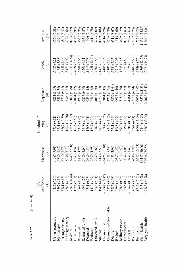
Tab

le 7

.25

(con

tinu

ed)

Lif

e sa

tisf

acti

on(1

)

Hap

pine

ss(2

)

Stan

dard

of

livin

g(3

)

Dep

ress

ed(4

)

Lon

ely

(5)

A

nxio

us(6

)

Upp

er s

econ

dary

.445

2 (7

.20)

.496

7 (7

.91)

.572

8 (9

.21)

–.62

24 (8

.97)

–.50

85 (7

.21)

–.37

73 (5

.38)

Non

tert

iary

.559

7 (8

.16)

.588

0 (8

.47)

.673

1 (9

.77)

–.65

02 (8

.38)

–.46

55 (5

.88)

–.39

94 (5

.13)

1st s

tage

tert

iary

.578

1 (9

.13)

.561

0 (8

.73)

.866

7 (1

3.59

)–.

6736

(9.4

2)–.

5457

(7.4

6)–.

3842

(5.3

3)2n

d st

age

tert

iary

.758

3 (8

.33)

.804

6 (8

.73)

1.12

44 (1

2.36

)–.

8300

(7.6

7)–.

8173

(7.0

2)–.

3794

(3.6

4)M

arri

ed.4

380

(14.

44)

.674

9 (2

2.00

).4

855

(15.

92)

–.20

97 (5

.79)

–.92

38 (2

4.54

)–.

0283

(0.7

9)C

ivil

part

ner

.157

6 (2

.32)

.296

9 (4

.34)

.181

6 (2

.68)

–.18

14 (2

.22)

–.48

24 (5

.70)

.072

2 (0

.92)

Sepa

rate

d–.

4863

(5.4

2)–.

3335

(3.7

5)–.

5256

(5.9

6).4

741

(4.8

8).5

793

(6.0

2).5

072

(5.2

3)Se

para

ted

(civ

il)–.

4096

(1.7

5)–.

5080

(2.0

4)–.

5818

(2.4

6).0

237

(0.0

9).0

299

(0.1

1)–.

3953

(1.3

7)D

ivor

ced

–.03

41 (0

.78)

.068

0 (1

.54)

–.17

68 (4

.01)

.059

1 (1

.15)

.141

5 (2

.78)

.109

0 (2

.14)

Wid

owed

–.14

42 (3

.09)

–.23

50 (4

.98)

–.13

57 (2

.90)

.250

2 (4

.68)

.695

1 (1

2.91

).3

614

(6.7

8)D

isso

lved

(civ

il)–.

3086

(2.3

1)–.

2289

(1.6

6)–.

6762

(4.9

0).4

097

(2.6

0).4

304

(2.8

6).6

273

(4.0

2)St

uden

t.1

985

(4.4

5).1

130

(2.5

3).2

913

(6.4

0)–.

0716

(1.3

3)–.

1473

(2.7

2).0

039

(0.0

8)U

nem

ploy

ed–.

9607

(16.

42)

–.64

75 (1

1.10

)1.

0584

(18.

32)

.580

4 (9

.17)

.448

5 (6

.96)

.431

4 (6

.70)

Une

mpl

oyed

(not

look

ing)

–.77

76 (9

.97)

–.54

43 (6

.88)

–.87

16 (1

1.03

).4

712

(5.4

1).5

392

(6.1

9).4

546

(5.2

0)D

isab

led

–.52

85 (8

.08)

–.40

53 (5

.96)

–.57

51 (8

.56)

.837

9 (1

1.64

).5

534

(7.5

3).6

312

(8.6

7)R

etir

ed.0

896

(2.4

4).0

587

(1.5

9)–.

1088

(2.9

7).0

927

(2.1

9).0

915

(2.0

5).1

516

(3.6

0)M

ilita

ry s

ervi

ce–.

2866

(0.9

6)–.

5011

(1.5

3)–.

6952

(2.1

6).5

182

(1.3

9).1

838

(0.4

5).8

609

(2.2

9)H

ome

wor

ker

–.00

85 (0

.22)

.003

1 (0

.08)

–.07

97 (2

.09)

.111

2 (2

.57)

.222

9 (4

.80)

.079

2 (1

.83)

Oth

er lf

–.07

47 (0

.76)

.046

1 (0

.47)

–.03

02 (0

.31)

.436

4 (4

.07)

.302

5 (2

.76)

.282

6 (2

.63)

Bad

hea

lth

.403

4 (5

.36)

.458

0 (5

.92)

.356

4 (4

.74)

–.51

58 (6

.54)

–.24

09 (3

.09)

–.29

97 (3

.75)

Fai

r he

alth

.871

6 (1

2.01

).9

745

(13.

05)

.800

8 (1

1.06

)–1

.067

6 (1

4.02

)–.

6548

(8.7

2)–.

7573

(9.8

5)G

ood

heal

th1.

4213

(19.

28)

1.51

47 (2

0.00

)1.

2440

(16.

95)

–1.6

578

(21.

35)

–.93

63 (1

2.25

)–1

.239

1 (1

5.85

)V

ery

good

hea

lth

1.91

83 (2

4.98

)2.

0326

(25.

82)

1.68

60 (2

2.05

)–2

.100

2 (2

5.47

)–1

.202

4 (1

4.76

)–1

.566

4 (1

9.04

)

Cut

1–4

.239

1–5

.239

4–4

.436

2–1

.791

1–.

6224

–2.1

631

Cut

2–3

.632

0–4

.533

6–3

.822

4.5

269

1.28

65.2

997

Cut

3–3

.004

3–3

.794

3–3

.121

12.

0986

2.57

591.

9788

Cut

4–2

.356

3–3

.090

1–2

.462

7C

ut5

–1.8

710

–2.5

543

–1.9

433

Cut

6–.

9569

–1.4

430

–1.0

441

Cut

7–.

4357

–.84

56–.

4025

Cut

8.4

154

.111

0–.

5434

Cut

91.

7241

1.46

421.

9403

Cut

102.

8699

2.67

673.

1896

Pse

udo

R2

.076

7.0

711

.088

5.0

961

.094

1.1

160

N34

,786

34,6

3834

,780

34,5

9234

,674

34,6

43A

ge m

in./m

ax.

49

53

46

39

50

33

Sou

rce:

Eur

opea

n So

cial

Sur

vey,

200

6 to

200

7.N

otes

: Exc

lude

d ca

tego

ries

: Bel

gium

, “si

ngle

,” “

very

bad

hea

lth,

” “p

aid

wor

k,”

and

“no

form

al e

duca

tion

.” (a

) All

thin

gs c

onsi

dere

d, h

ow sa

tisfi

ed

are

you

wit

h yo

ur li

fe a

s a

who

le n

owad

ays?

(b) A

nd h

ow s

atis

fi ed

are

you

wit

h yo

ur p

rese

nt s

tand

ard

of li

ving

? P

leas

e an

swer

usi

ng th

is c

ard,

whe

re z

ero

mea

ns “

extr

emel

y di

ssat

isfi e

d” a

nd te

n m

eans

“ex

trem

ely

sati

sfi e

d.”

Tak

ing

all t

hing

s to

geth

er, h

ow h

appy

wou

ld y

ou s

ay y

ou a

re?

(Ext

rem

ely

unha

ppy

� 0

to e

xtre

mel

y ha

ppy

� 1

0.) U

sing

this

car

d, p

leas

e te

ll m

e ho

w m

uch

of th

e ti

me

duri

ng th

e pa

st w

eek

(a) y

ou fe

lt d

epre

ssed

; (b)

you

felt

lone

ly; a

nd (c

) you

felt

anx

ious

. (N

one

or

alm

ost n

one

of th

e ti

me,

som

e of

the

tim

e, m

ost o

f th

e ti

me,

or

all o

r al

mos

t all

of th

e ti

me.

)

Table 7.26 Well- being rankings: 2006–2007 European Social Surveys

Denmark France Great Britain

1) Life satisfaction 1 14 92) Happiness 1 10 73) Standard of living 1 11 74) Depressed 18 11 125) Lonely 19 6 126) Anxious 17 8 12

Table 7.27 Happiness and unhappiness rankings: 2006–2007 European Social Surveys

Denmark France Great Britain

Happiness ranks You were happy? 10 4 5 You enjoyed life? 4 2 5 You had a lot of energy? 11 7 17 You felt calm and peaceful? 1 16 18 You felt really rested when you woke up in the morning? 12 15 19Unhappiness ranks You felt that everything you did was an effort? 7 13 10 Your sleep was restless? 9 7 2 You felt sad? 17 13 12 You could not get going? 11 19 6 You felt tired? 8 6 3 You felt bored? 17 13 5

Fig. 7.3 Life satisfaction and the unemployment rate (2003)


from the 1995 through 2000 WVS; the slope of the function for Western countries is approximately horizontal.

There is a small body of literature that uses SWB data across countries and through time to estimate a “misery index.” Di Tella, McCulloch, and Oswald (2001, 2003) and Di Tella and MacCulloch (2007) use life satisfac-tion data to show that people are happier when both infl ation and unemploy-

Fig. 7.4 Life satisfaction and infl ation (2003 HICP)

Fig. 7.5 Life satisfaction and GDP per capita


ment are low. They all fi nd that unemployment depresses well- being more than does infl ation. Di Tella and MacCulloch (2007) suggest that left- wing individuals care more about unemployment relative to infl ation than do right- wingers. Wolfers (2003) has also shown that greater macro volatility undermines well- being.

Table 7.28 uses aggregate life satisfaction data from the country∗year cell of the World Database of Happiness, with the dependent variable as the score on a 4- step scale. Results are reported without a lagged dependent variable in columns (1) and (3) and with one added in columns (2) and (4), but this has little effect on the results. In columns (3) and (4), GDP per capita is added in U.S. dollars but is always insignifi cant once controls for unemployment and infl ation are included. The rank ordering of countries once again is lowest- ranked France, then the United Kingdom, followed by the United States, and then highest- ranked Denmark. Both unemployment and infl ation lower happiness. A 1 percentage point increase in unemploy-ment has a larger impact than a 1 percentage point increase in infl ation in all four columns. If GDP per capita is included without controls for infl ation or unemployment but with country and year dummies, it enters positively and signifi cantly. If an additional term is included, where GDP is interacted with a poor country dummy, the results were as seen in table 7.29, with t- statistics in parentheses.21 Both terms are signifi cant and positive, but the slope for

Fig. 7.6 1995 to 2000 World Values Survey result

21. “Poor” is defi ned here as having 2004 GDP per capita of less than $20,000, which includes the Czech Republic ($6,263), Hungary ($5,626), Italy ($19,506), Mexico ($6,006), Poland ($5,032), Portugal ($11,090), Slovakia ($4,483), and Spain ($15,403)—GDP per capita in U.S. dollars in parentheses.


the richer countries is less steep than found for the poorer countries—there is diminishing marginal utility of income. This is the Easterlin effect, and it does suggest that rising GDP per capita raises happiness less for devel-oped than for developing countries, which is consistent with the fi ndings of Deaton (2008), who argues that “it is not true that there is some critical level of GDP per capita above which income has no further effect on hap-piness” (2008, 16– 17). It is also consistent with the fi ndings of Helliwell (2003), who uses data from the fi rst three sweeps of the WVS and fi nds that in a life satisfaction equation across countries, “national average income also has diminishing returns, since the logarithm of average per capita income takes a positive coefficient, while the square takes a negative coefficient” (345). This result is different from the fi ndings of Easterlin (1974, 1995) that happiness does not increase for long time spans, despite large increases

Table 7.28 Macrolife satisfaction: 1973–2006 (ordered logits)

(1) (2) (3) (4)

Life satisfactiont–1 .5713 (13.83) .5689 (13.64)Infl ationt –.0056 (3.87) –.0029 (2.32) –.0061 (4.11) –.0031 (2.37)Unemploymentt –.0126 (6.26) –.0046 (2.77) –.0119 (5.69) –.0046 (2.63)GDPt .000002 (1.46) .00001 (0.51)Austria –.0819 (3.20) –.0458 (2.24) –.0783 (3.04) –.0452 (2.19)Belgium –.0266 (1.46) –.0181 (1.26) –.0250 (1.36) –.0178 (1.22)Czech Republic –.3133 (9.38) –.1284 (4.18) –.2737 (5.59) –.1175 (2.81)Denmark .3816 (20.73) .1710 (7.94) .3707 (18.67) .1688 (7.64)Finland .0484 (1.86) .0248 (1.21) .0493 (1.90) .0252 (1.22)France –.2940 (16.01) –.1253 (6.64) –.2920 (15.85) –.1253 (6.61)Germany –.1334 (7.17) –.0563 (3.65) –.1333 (7.16) –.0566 (3.66)Greece –.4725 (21.48) –.1937 (7.31) –.4474 (16.05) –.1876 (6.41)Hungary –.6310 (18.77) –.2768 (7.30) –.5785 (11.73) –.2640 (5.73)Ireland .0764 (3.88) .0329 (2.10) .0847 (4.11) .0360 (2.17)Italy –.3445 (18.72) –.1375 (6.77) –.3346 (17.06) –.1354 (6.50)Japan –.5266 (23.77) –.2317 (8.27) –.5519 (19.79) –.2403 (7.45)Luxembourg .0779 (3.55) .0475 (2.71) .0497 (1.71) .0395 (1.71)Mexico –.2705 (6.53) –.2517 (4.32) –.2167 (3.89) –.2371 (3.63)Netherlands .1835 (9.50) .0792 (4.68) .1844 (9.53) .0799 (4.60)Poland –.2952 (6.80) –.1135 (2.97) –.2511 (4.76) –.1014 (2.27)Portugal –.5259 (24.67) –.2211 (8.11) –.4917 (15.47) –.2130 (6.64)Slovakia –.4588 (10.64) –.1769 (4.34) –.4112 (7.63) –.1641 (3.45)Spain –.1276 (5.30) –.0528 (2.69) –.1075 (3.89) –.0472 (2.10)Sweden .1590 (6.03) .0736 (3.36) .1544 (5.81) .0726 (3.29)U.S. .1674 (5.64) .1137 (4.02) .1465 (4.46) .1081 (3.56)

Constant 3.1310 1.4209 3.2277 1.4230Adjusted R2 .9375 .9631 .9376 .9630N 457 423 455 421

Source: World Database of Happiness and OECD, 1973 to 2006.Notes: The U.K. is excluded category. T- statistics in parentheses. Equations also include thirty- one year dummies. GDP is per capita in U.S. dollars. Data on GDP unavailable in 2006 for Czech Republic and Ireland.


Table 7.29 Life satisfaction equations: 1972–2006 Eurobarometers

Without a lagged

dependent variable With a lagged

dependent variable

GDPt .000016 (11.84) .00000247 (2.12)GDP poor countryt .0000287 (6.46) .00000746 (2.14)

in income. Consistent with this result is the fact that happiness levels for a number of E.U. countries have increased over time. Indeed, in the pooled microdata fi les of the Eurobarometers from 1973 to 2006, if we simply regress life satisfaction in an OLS on a time trend only, there is a signifi cant upward trend in life satisfaction for ten countries—Denmark, the United Kingdom, France, Finland, Ireland, Luxembourg, the Netherlands, Spain, Sweden, and Italy. There is a negative trend for Portugal, Germany, and Belgium and no signifi cant trend for Austria and Greece.22

Table 7.30 uses microdata on over 700,000 individuals from fi fteen coun-tries for which I have long- time series- of- infl ation data dating back to the 1950s (Austria, Belgium, Denmark, Finland, France, Germany, Greece, Ireland, Italy, the Netherlands, Norway, Portugal, Spain, Sweden, and the United Kingdom), drawn from the Eurobarometers from 1973 to 2006 and reported in Blanchfl ower (2007). As in table 7.28, which uses macrodata, controls are included for the unemployment rates and the infl ation rate, but here, standard errors are clustered at the country∗year cell. Once again both macrovariables enter negatively, and the ranking is Denmark, then the United Kingdom, and fi nally lowest- ranked France. Column (2) adds the variable refl ecting the average annual infl ation experience of each indi-vidual in our sample, given their age, their country, and the year the life satisfaction survey was conducted; this term is insignifi cant. Column (3) substitutes the average annual experience term for the highest annual infl a-tion rate experienced by each individual over their adult life. This term is negatively signed and signifi cant, and its inclusion has essentially no effect on either the coefficients of infl ation or unemployment. An individual who has experienced high infl ation in the past has lower happiness today, even holding constant today’s infl ation and unemployment rates. Unemployment appears to be more costly than infl ation in terms of its impact on well- being. In Blanchfl ower (2007), I used these data to estimate a misery- index, which measures the relative effect of a 1 percentage point increase in unemploy-ment compared with a 1 percentage point increase in infl ation. The estimates imply individuals weight the loss from unemployment 1.6 times more than

22. Data are available for 1973 to 2006 for Belgium, France, Denmark, Germany, Ireland, Italy, Luxembourg, Netherlands, and the United Kingdom; for 1981 to 2006 for Greece; for 1985 to 2006 for Portugal and Spain; and from 1995 to 2006 for Austria, Finland, and Sweden.

Tab

le 7

.30

Mic

rolif

e sa

tisf

acti

on: E

urop

e, 1

973–

2006

(ord

ered

logi

ts)

Age

� 4

0A

ge �

40

(1)

(2

)

(3)

(4

)

(5)

Infl a

tion

t–.

0094

(5.1

6)–.

0095

(5.1

8)–.

0096

(5.2

5)–.

0102

(4.8

3)–.

0128

(5.8

9)U

nem

ploy

men

t rat

e t–.

0114

(5.8

2)–.

0115

(5.8

8)–.

0119

(6.0

5)–.

0109

(5.7

1)–.

0081

(4.2

0)A

vera

ge in

fl ati

on e

xper

ienc

e–.

0010

(1.0

2)H

ighe

st in

fl ati

on e

xper

ienc

e–.

0001

(3.4

4)–.

0002

(2.6

2)–.

0000

3 (2

.85)

Age

–.01

33 (1

6.42

)–.

0133

(16.

38)

–.01

34 (1

6.74

)–.

0067

(1.8

7)–.

0048

(3.8

3)A

ge2

.000

1 (1

8.68

).0

001

(18.

58)

.000

1 (1

9.11

)–.

0000

(0.0

1).0

0007

(7.4

1)M

ale

–.03

27 (1

0.48

)–.

0328

(10.

43)

–.03

29 (1

0.51

)–.

0424

(11.

94)

–.02

30 (5

.69)

16–1

9 yr

s. s

choo

ling

.087

3 (1

7.72

).0

873

(17.

73)

.087

1 (1

7.80

).0

723

(10.

70)

.093

1 (1

8.85

)20

� y

rs. s

choo

ling

.166

4 (2

6.12

).1

665

(26.

13)

.166

4 (2

6.23

).1

530

(21.

10)

.166

6 (2

1.92

)St

ill s

tudy

ing

.117

8 (7

.88)

.117

4 (7

.84)

.117

4 (7

.82)

.112

7 (9

.02)

–.00

80 (0

.11)

Mar

ried

.118

6 (1

9.86

).1

185

(19.

84)

.118

9 (1

9.92

).1

325

(20.

30)

.127

5 (1

7.81

)L

ivin

g as

mar

ried

.048

1 (7

.38)

.048

3 (7

.38)

.049

6 (7

.61)

.056

9 (8

.20)

.040

6 (3

.65)

Div

orce

d–.

1621

(20.

04)

–.16

23 (2

0.05

)–.

1622

(20.

05)

–.16

93 (1

5.76

)–.

1415

(14.

86)

Sepa

rate

d–.

2065

(19.

13)

–.20

65 (1

9.12

)–.

2061

(19.

12)

–.20

85 (1

3.83

)–.

1839

(12.

83)

Wid

owed

–.08

66 (1

3.17

)–.

0864

(13.

09)

–.08

52 (1

2.95

)–.

0938

(3.3

5)–.

0723

(9.7

7)Se

lf- e

mpl

oyed

.005

7 (1

.22)

.005

7 (1

.20)

.005

6 (1

.19)

.029

5 (4

.69)

–.00

97 (1

.71)

Hom

e w

orke

r–.

0243

(4.8

0)–.

0244

(4.8

0)–.

0244

(4.8

1)–.

0293

(4.5

0)–.

0205

(3.4

3)St

uden

t.0

710

(4.9

0).0

713

(4.9

2).0

715

(4.9

3).0

589

(4.9

4).0

487

(0.7

3)R

etir

ed–.

0395

(6.8

8)–.

0394

(6.8

4)–.

0395

(6.8

9)–.

1463

(6.2

3)–.

0348

(5.9

6)U

nem

ploy

ed–.

3657

(29.

77)

–.36

58 (2

9.74

)–.

3660

(29.

71)

–.35

74 (3

0.25

)–.

3909

(24.

68)

Aus

tria

–.09

56 (4

.17)

–.09

69 (3

.45)

–.09

04 (3

.96)

–.07

20 (2

.65)

–.11

42 (4

.90)

Bel

gium

–.08

07 (0

.23)

–.09

55 (4

.17)

–.08

07 (4

.39)

–.04

32 (2

.11)

–.11

64 (5

.99)

Den

mar

k.3

220

(21.

96)

.321

2 (2

1.82

).3

206

(21.

78)

.351

5 (2

1.58

).2

969

(19.

72)

Fin

land

–.00

01 (0

.00)

.001

4 (0

.07)

.003

2 (0

.16)

.039

7 (1

.60)

–.02

83 (1

.49)

Fra

nce

–.32

71 (2

3.35

)–.

3254

(23.

29)

–.32

54 (2

2.99

)–.

3044

(17.

94)

–.34

40 (2

5.36

)

Tab

le 7

.30

(con

tinu

ed)

Age

� 4

0A

ge �

40

(1)

(2

)

(3)

(4

)

(5)

Ger

man

y–.

2286

(19.

35)

–.22

97 (1

9.18

)–.

2229

(18.

85)

–.22

55 (1

7.82

)–.

2289

(17.

34)

Gre

ece

–.45

96 (2

0.71

)–.

4512

(18.

89)

–.44

85 (2

0.32

)–.

3443

(15.

86)

–.55

00 (2

0.14

)Ir

elan

d.0

524

(3.5

0).0

540

(3.6

1).0

549

(3.6

8).0

471

(2.8

3).0

651

(4.0

1)It

aly

–.34

34 (1

7.47

)–.

3374

(15.

85)

–.33

06 (1

6.34

)–.

2789

(12.

53)

–.38

50 (2

0.09

)N

ethe

rlan

ds.1

199

(10.

55)

.117

9 (1

0.12

).1

181

(10.

33)

.154

9 (1

1.70

).0

869

(7.2

3)N

orw

ay.1

072

(3.4

7).1

064

(3.4

4).1

057

(3.4

2).1

423

(4.6

5).0

757

(2.3

0)Po

rtug

al–.

4979

(21.

41)

–.49

39 (2

1.13

)–.

4973

(21.

47)

–.37

46 (1

5.68

)–.

6047

(25.

23)

Spai

n–.

1240

(7.4

1)–.

1206

(7.1

0)–.

1200

(7.1

4)–.

0794

(3.9

8)–.

1632

(9.7

9)Sw

eden

.105

7 (8

.12)

.105

4 (8

.07)

.105

4 (8

.04)

.138

6 (7

.04)

.082

1 (6

.27)

Con

stan

t3.

5198

3.52

623.

5264

3.43

153.

2963

N70

3,17

270

3,17

270

3,17

233

2,20

237

0,97

0R

2

.154

9

.154

9

.155

0

.148

1

.163

9

Sou

rce:

Eur

obar

omet

ers,

197

3 to

200

6, a

nd B

lanc

hfl o

wer

(200

7).

Not

es: E

xclu

ded

cate

gori

es a

re th

e U

.K.,

“em

ploy

ee,”

“no

chi

ldre

n,”

“lef

t sch

ool b

efor

e ag

e 15

,” a

nd “

sing

le.”

All

equa

tion

s in

clud

e tw

enty

yea

r du

mm

ies.

St

anda

rd e

rror

s ar

e cl

uste

red

by c

ount

ry a

nd y

ear.

“A

vera

ge in

fl ati

on e

xper

ienc

e” r

efer

s to

the

ave

rage

ann

ual i

nfl a

tion

rat

e ex

peri

ence

d by

an

indi

vidu

al

over

thei

r lif

e to

the

surv

ey d

ate.

“H

ighe

st in

fl ati

on e

xper

ienc

ed”

refe

rs to

the

high

est a

nnua

l infl

ati

on r

ate

expe

rien

ced

by a

n in

divi

dual

ove

r th

eir

life

to th

e su

rvey

dat

e.


the loss in well- being from infl ation.23 Columns (4) and (5) of the table pro-vide separate estimates for those younger than forty years old and for those age forty and older. Interestingly, for the younger group, the misery- index is close to 1.4, whereas for the older group, it is approximately 2.1, while the size of the loss of happiness for the unemployed is similar.24 Interestingly, the highest infl ation term, which is negative and signifi cant in both cases, is much larger in size in the former case, although its mean is much lower (20.2 and 116.2, respectively).

In table 7.31 I explore the impact of the macroeconomy on individual happiness and life satisfaction using self- reported views on unemployment, infl ation, and inequality from three recent Eurobarometers from 2006 and 2007. The results are very similar to those based on using the macrodata; we also have evidence that inequality lowers happiness. In the fi rst column the results from estimating a series of ordered logits are reported, with 4- step happiness as the dependent variable. In addition to the standard con-trols of labor market and marital status, schooling, gender, age, and country dummies, plus a number of additional controls not available in other data fi les were used. First, if the respondent is a member of a minority group, as well as if they are not part of the majority but do not associate them-selves with a particular group, they enter signifi cantly and negative with the effect three times larger. Second, controls are included to distinguish whether they owned their house outright or with a mortgage, both which enter signifi cantly positive. Third, I include a control identifying whether the respondent belonged to a religious organization, which is also signifi -cant and positive. Fourth, following Di Tella and MacCulloch (2005) and Alesina, Di Tella, and MacCulloch (2004), I include controls for an indi-vidual’s political views on a scale from one (left wing) to ten (right wing) and show that right- wingers are happiest. Finally, I include three vari-ables based on an individual’s response to a question asking what top-ics “worry you the most?” I include responses relating to unemployment, inequality, and the cost of living (infl ation); multiple responses are pos-sible. Unemployment and infl ation lowers happiness, as does inequality, following Alesina, Di Tella, and MacCulloch (2004) and Blanchfl ower and Oswald (2004a). Column (2) uses data from Eurobarometer number 66.1,

23. The misery- index is calculated in Blanchfl ower (2007) as the coefficient of the unemploy-ment rate plus the loss for the unemployed themselves, divided by the coefficient on the infl ation rate. The loss to the individual from being unemployed can be calculated from the coefficient of being “unemployed” in a life- satisfaction microregression like the one reported in column (1) of table 7.18: estimated with OLS to keep the units consistent, we get – 0.3657. The entire well- being cost of a 1 percentage point increase in the unemployment rate is therefore given by the sum of two components. Combining the two, we have 0.0114 � 0.0036 � 0.0147 as society’s overall well- being cost for a 1 percentage point rise in the unemployment rate divided by 0.0094. The implication is that the well- being cost of a 1 percentage point increase in the unemployment rate equals the loss brought about by an extra 1.56 percentage points of infl ation.

24. Calculated as (0.0102 � 0.0036)/ 0.0109 � 1.27 and (0.0128 � 0.0039)/ 0.0081 � 2.06, respectively.

Table 7.31 Happiness, life satisfaction, and views on the macroeconomy, 2006–2007 (ordered logits)


Inequality (current) –.1976 (5.77)Unemployment (current) –.0787 (2.71) –.0745 (2.79)Infl ation (current) –.2313 (8.40) –.1468 (4.83)Infl ation (equal) –.0409 (0.97)Infl ation (higher) –.0671 (1.83)Unemployment (equal) –.1895 (4.80)Unemployment (higher) –.2402 (6.56)Age –.0973 (19.20) –.0785 (16.84) –.0871 (14.48)Age2 .0008 (16.43) .0007 (15.99) .0008 (13.65)Male –.1655 (6.00) –.1187 (4.60) –.0566 (1.83)ALS � 16 –.0958 (0.66) .3097 (2.84) –.3417 (0.82)ALS 16–19 .1883 (1.30) .6316 (5.72) –.2154 (0.52)ALS � 20 .3747 (2.55) .8830 (7.87) .0368 (0.09)Unemployed –.7356 (10.43) –.6970 (11.01) –.8683 (10.77)Retired –.1756 (3.11) .0142 (0.27) –.1487 (2.19)Married .8203 (16.61) .3283 (7.18) .3544 (6.48)Remarried .6441 (6.42) .2989 (3.16) .3703 (3.28)Living as married .4075 (6.88) .1736 (3.10) .1033 (1.55)Previously lived together –.2089 (2.69) –.2262 (3.21) –.4206 (5.10)Divorced –.1563 (2.35) –.2834 (4.50) –.4249 (5.64)Separated –.5704 (5.15) –.3983 (3.71) –.4337 (3.49)Widowed –.4460 (6.80) –.2379 (3.89) –.3670 (4.85)Austria –.9599 (10.46) .0404 (0.55) –.0304 (0.35)Bulgaria –3.1762 (33.98) –2.2106 (30.93) –2.2350 (23.42)Cyprus –1.0438 (9.06) .3658 (3.74) .3694 (2.77)Czech Republic –1.2175 (13.65) –.3675 (5.08) –.3712 (4.40)Denmark .4515 (4.90) 1.9123 (23.45) 1.7403 (18.61)East Germany –1.2621 (11.05) –.5185 (5.31) –.4315 (3.97)Estonia –1.6008 (17.00) –.6161 (8.28) –.7205 (7.96)Finland –.4786 (5.31) .7295 (9.88) .4965 (5.88)France –.2727 (3.00) –.0309 (0.42) –.2405 (2.65)Greece –1.2132 (12.85) –.6965 (9.42) –1.0286 (12.59)Hungary –1.6718 (17.61) –1.5970 (22.32) –1.5296 (17.90)Ireland .2515 (2.73) .8377 (11.11) .7815 (8.75)Italy –1.1559 (12.49) –.3288 (4.48) –.6513 (7.02)Latvia –1.7255 (18.56) –.9410 (12.72) –1.1391 (13.10)Lithuania –1.8129 (19.28) –1.0639 (14.30) –1.0678 (11.90)Luxembourg –.0565 (0.51) 1.1205 (11.56) 1.2979 (10.77)Malta –.5982 (5.19) .2136 (2.13) .3762 (2.96)Netherlands .0978 (1.07) 1.2924 (16.78) 1.1640 (13.24)Poland –1.0093 (10.85) –.5752 (7.84) –.5261 (5.64)Portugal –.9639 (10.32) –1.0027 (13.87) –1.0446 (10.94)Romania –2.4141 (25.56) –1.7300 (24.31) –1.5874 (15.49)Slovakia –1.8201 (19.67) –.8210 (11.21) –.8749 (10.59)Slovenia –.6665 (7.25) .2936 (4.04) .1955 (2.26)Spain –.6784 (7.34) .4474 (6.07) .0516 (0.51)Sweden –.1260 (1.38) 1.2562 (16.46) 1.1273 (12.91)U.K. .1592 (1.84) .7696 (11.20) .8118 (9.32)


which uses a 4- step life satisfaction dependent variable and confi rms that both unemployment and infl ation lowers pay—information on inequality is available in that survey.25

Column (3) also uses 4- step data on life satisfaction from a 2007 Euro-barometer, number 67.2, with slightly different attitudinal questions. Once again, the unemployed have lower life satisfaction; happiness is U- shaped in age and higher for the married and for those who own their own house. It is especially high in Denmark and low in Bulgaria. The main difference in



West Germany –.8584 (9.22) .2374 (3.21) .3455 (3.99)Member religious org. .2927 (5.20) .0455 (1.17)Minority group –.2695 (5.78)No group –.1113 (3.52)Own house (outright) .2112 (6.11) .3899 (12.65) .2414 (6.23)Own house (mortgage) .1099 (2.85) .3356 (9.33) .3188 (7.36)Left wing (1–2) .0478 (0.75) .0123 (0.21) .1210 (1.67)Left (3–4) .0028 (0.05) .1584 (3.17) .2116 (3.36)Center (5–6) .0843 (1.74) .2392 (5.35) .2259 (3.88)Right (7–8) .1413 (2.60) .3746 (7.49) .3792 (5.98)Right wing (9–10) .3454 (5.20) .4856 (8.31) .5561 (7.58)

Cut1 –7.1023 –4.1532 –5.6338Cut2 –4.8577 –2.2430 –3.6509Cut3 –1.4631 .8395 –.4712

N 26,526 29,017 20,472Pseudo R2 .1319 .1294 .1297

Source: Column (1) � Eurobarometer number 66.3: European Social Reality, November to December 2006 (ICPSR study number 4528). Column (2) � Eurobarometer number 66.1: European Values and Societal Issues, Mobile Phone Use, and Farm Animal Welfare, Septem-ber to October 2006 (ICPSR study number 21281). Column (3) � Eurobarometer number 67.2: European Union Enlargement, Personal Data Privacy, National Economy and Scientifi c Research, April to May 2007 (ICPSR study number 21160).Notes: Excluded categories: Belgium; “responsible for ordinary shopping and housework,” “unmarried, having previously lived with a partner,” “no formal education,” “refused to an-swer left/right scale,” and “majority group.” All equations also include fi fteen occupation dummies. T- statistics in parentheses. Survey questions: Q1. On the whole, are you very satis-fi ed, fairly satisfi ed, not very satisfi ed, or not at all satisfi ed with the life you lead? Q2. Do you think that in (OUR COUNTRY), the infl ation rate in 2006 was higher, lower, or equal to the one in 2005? Q3. Do you think that in (OUR COUNTRY), the unemployment rate in 2006 was higher, lower, or equal to the one in 2005? Q4. Taking all things together, would you say you are very happy, quite happy, not very happy, or not at all happy? Q5. Which topics worry you the most?: (a) unemployment, (b) the cost of living (infl ation), (c) the gap between the rich and the poor (inequality). Q6. In political matters people talk of “the left” and “the right.” How would you place your views on this scale? (1 [left] to 10 [right].)

25. Similar results are also found using Eurobarometer number 64.1, which does not contain details of home ownership.


column (3) is that now, the macro controls relate to whether the respondent believes that infl ation is lower than, equal to, or higher than it was a year earlier. Once again, happiness is lower when the respondent reports that infl ation or unemployment is higher. Unemployment, infl ation, and inequal-ity all appear to lower happiness and life satisfaction.

7.6 Predictions and Expectations

I recall John Abowd saying to me at a very early seminar given at the Na-tional Bureau of Economic Research that the crucial test for happiness data is whether or not it has any predictive power. Little work has so far been done on this question, but in some recent work I found that life satisfaction levels in Eastern European countries is a good predictor of migration fl ows to the United Kingdom. On May 1, 2004, the so- called A8 accession coun-tries (the Czech Republic, Estonia, Hungary, Latvia, Lithuania, Poland, Slovakia, and Slovenia) joined the European Union.26 Citizens from the A8 nations obtained free movement and the right to work in the United King-dom, Ireland, and Sweden as of May 1, 2004.27 Gilpin et al. (2006) examined data for the United Kingdom drawn from the Worker Registration Scheme (WRS), which registers the A8 workers, and computed the number of WRS registrations as a percentage of the home country population, which showed it is correlated with GDP and unemployment. Gilpin et al. found that coun-tries with the lowest GDP per head, such as Lithuania (€2,500), are more likely to be registered on the U.K. WRS than those from countries with a higher GDP, such as Slovenia (€11,400).28 The propensity to migrate is even more highly correlated with life satisfaction than it is with GDP per capita (Blanchfl ower and Shadforth 2009).

Of interest is whether life satisfaction or happiness is correlated with people’s expectations of the economic situation. It turns out that they are. Respondents in thirteen separate Eurobarometers for the period of 1995 to 2006 were asked the following questions.

What are your expectations for the next twelve months: will the next twelve months be better, worse, or the same when it comes to a) your life in general, b) the economic situation in (our country), c) the fi nancial situation of your household, d) the employment situation in (our coun-try), and e) your personal job situation?

Data are available on fi fteen countries for all twelve years (Austria, Belgium, Denmark, Finland, France, Germany, Greece, Ireland, Italy, Luxembourg,

26. In addition, Malta and (South) Cyprus also joined the European Union at that date. Bulgaria and Romania joined the European Union on January 1, 2007.

27. Finland, Greece, Portugal, and Spain opened their labor markets to these workers on May 1, 2006, while Italy followed in late July 2006. Five other countries (Belgium, Denmark, France, the Netherlands, and Luxembourg) alleviated restrictions in 2006 (Zaiceva 2006).

28. Expressed as Euros per inhabitant at 1995 exchange rates and prices.


the Netherlands, Portugal, Spain, Sweden, and the United Kingdom). Data for the fi fteen accession and candidate countries (Republic of Cyprus, Czech Republic, Estonia, Hungary, Latvia, Lithuania, Malta, Poland, Slovakia, Slovenia, Bulgaria, Romania, Turkey, Croatia, and Cyprus [Turkish Cypriot Community]) are present for only 2004 to 2006. In eight separate surveys, respondents were also asked about their expectations for themselves ten years hence—“In the course of the next fi ve years, do you expect your per-sonal situation to improve, to stay about the same, or to get worse?” Life satisfaction is further reported in a subset of these surveys. We examine three of these responses here.

Table 7.32 reports the results of estimating ordered logits for parts b, d, and d of the question, as well as for life fi ve years ahead. The dependent variable is coded as one if the response was “worse,” two if it was “the same,” and three if it was “better,” so positive coefficients should be interpreted once again as suggesting that the variable raises the probability of life improving. Column (1) and (2) of table 7.32 relates to the individual’s views on the eco-nomic situation, columns (3) and (4) to the employment situation, columns (5) and (6) to their life over the following twelve months, and columns (7) and (8) for life over the following fi ve years. In each case, separate results are provided with and without three life satisfaction controls derived from the standard 4- category life satisfaction variable. Happiness enters signifi cantly and positively in each of these equations. This is similar to fi ndings by Guven (2007), who found by using data from the Netherlands and Germany that happiness increases savings and decreases expenditures, and that the mar-ginal propensity to consume is lower for the happy people. Happy people, Guven also found, (a) are more risk averse in fi nancial decisions, (b) expect to live longer, (c) are more concerned about the future than the present, (d) expect lower prices in the future, (e) are less likely to smoke, and (f) do not desire to move within a country.29

There is a common pattern in the control variables across all eight specifi -cations. Optimism (a) rises with educational attainment, (b) is U- shaped in age, (c) is lower for the married, the widowed, and the unemployed, and (d) is higher when the level of current happiness is greater. The country ranking in relation to people’s views on the economic and employment situations is once again France, then the United Kingdom, and then Denmark. The British, though, are especially optimistic that their life will improve, and the Danish are now less optimistic than the French. Happier people, it turns out,

29. Guven (2007) examined data on prices only for the Netherlands using data from the Dutch National Bank Household Survey, which is a panel of about 4,500 individuals from 1993 to 2006. Data on price expectations are of particular interest to macropolicy makers. Guven found that happier people expect lower prices than unhappy people for the next year and also in fi ve years’ time. Questions asked were (a) “Do you expect prices in general to rise, to remain the same, or to go down in the next 12 months? 1 � go down, 2 � remain the same, 3 � rise,” and (b) “By what percentage do you expect prices in total to have risen after 5 years?”

Tab

le 7

.32

Eco

nom

ic, e

mpl

oym

ent,

and

life

exp

ecta

tion

s in

Eur

ope:

199

5–20

06 E

urob

arom

eter

s (o

rder

ed lo

gits

)

Eco

nom

ic s

itua

tion

Em

ploy

men

t sit

uati

onL

ife

one

year

ahe

adL

ife

fi ve

year

s ah

ead

(1)

(2

)

(3)

(4

)

(5)

(6

)

(7)

(8

)

Fra

nce

–.19

92 (8

.00)

–.16

45 (5

.65)

.211

2 (8

.41)

.253

2 (8

.65)

.516

6 (2

0.17

).6

714

(22.

18)

.241

9 (7

.76)

.304

5 (8

.99)

Den

mar

k.2

793

(11.

31)

.164

0 (5

.68)

.671

0 (2

6.70

).4

432

(15.

09)

.474

1 (1

8.48

).2

439

(8.0

1).5

509

(17.

42)

.342

7 (9

.88)

U.K

..1

664

(7.2

3).0

751

(2.8

0).5

437

(23.

41)

.422

3 (1

5.64

).8

461

(35.

52)

.794

4 (2

8.28

).8

284

(28.

01)

.759

9 (2

3.68

)N

ot v

ery

sati

sfi e

d.5

787

(22.

91)

.531

8 (2

1.01

).9

013

(34.

32)

.838

0 (2

8.38

)F

airl

y sa

tisfi

ed

1.09

71 (4

4.84

).9

678

(39.

53)

1.84

23 (7

2.14

)1.

7548

(61.

65)

Ver

y sa

tisfi

ed

1.37

50 (5

2.90

)1.

2523

(48.

21)

2.32

65 (8

5.19

)2.

1457

(69.

87)

Age

–.02

47 (1

6.31

)–.

0177

(10.

33)

–.02

60 (1

7.03

)–.

0187

(10.

89)

–.04

54 (2

9.01

)–.

0338

(18.

99)

–.07

17 (3

6.07

)–.

0623

(29.

09)

Age

2.0

002

(12.

98)

.000

1 (7

.84)

.000

2 (1

3.53

).0

001

(8.3

0).0

002

(14.

87)

.000

1 (6

.75)

.000

4 (1

9.36

).0

002

(13.

11)

Mal

e.1

379

(15.

73)

.134

7 (1

3.62

).0

694

(7.8

6).0

791

(7.9

6)–.

0424

(4.6

8)–.

0443

(4.3

0)–.

0015

(0.1

4).0

119

(1.0

1)A

LS

16–1

9.1

058

(9.3

5).0

659

(5.1

3).1

005

(8.7

8).0

713

(5.5

0).2

280

(19.

58)

.165

0 (1

2.42

).1

279

(9.1

3).0

714

(4.7

7)A

LS

20�

.268

4 (2

0.75

).1

946

(13.

26)

.256

0 (1

9.61

).1

970

(13.

31)

.443

9 (3

3.20

).3

216

(21.

07)

.352

1 (2

1.82

).2

552

(14.

80)

Still

stu

dyin

g–.

1670

(2.2

5)–.

1396

(1.8

5)–.

0469

(0.6

3)–.

0399

(0.5

3).0

261

(0.3

4).0

510

(0.6

6)–.

1002

(1.2

0)–.

0596

(0.7

1)H

omem

aker

–.03

54 (1

.93)

.006

6 (0

.32)

–.02

79 (1

.51)

.015

0 (0

.72)

–.11

02 (5

.83)

–.06

77 (3

.14)

–.14

06 (6

.12)

–.10

88 (4

.44)

Stud

ent

.414

1 (5

.51)

.322

4 (4

.20)

.268

1 (3

.53)

.211

8 (2

.75)

.202

5 (2

.62)

.034

0 (0

.43)

.235

6 (2

.75)

.024

7 (0

.29)

Une

mpl

oyed

–.17

22 (8

.46)

–.04

28 (1

.85)

–.16

66 (8

.14)

–.06

00 (2

.58)

–.06

74 (3

.15)

.173

8 (7

.08)

–.34

99 (1

3.55

)–.

1498

(5.3

9)R

etir

ed–.

0892

(5.1

4)–.

0679

(3.4

7)–.

0604

(3.4

3)–.

0479

(2.4

3)–.

2201

(12.

24)

–.20

62 (1

0.16

)–.

2226

(10.

02)

–.18

28 (7

.69)

Far

mer

–.25

91 (7

.36)

–.20

83 (5

.22)

–.18

74 (5

.37)

–.18

56 (4

.68)

–.42

08 (1

1.53

)–.

3427

(8.3

2)–.

4239

(9.5

9)–.

3726

(7.9

8)F

ishe

rman

–.09

87 (0

.50)

–.13

20 (0

.60)

.200

0 (1

.02)

.195

2 (0

.90)

–.02

21 (0

.11)

–.02

60 (0

.11)

–.55

45 (2

.20)

–.57

13 (2

.13)

Pro

fess

iona

l.1

447

(4.1

3).1

020

(2.5

8).0

805

(2.3

0).0

583

(1.4

7).3

413

(9.3

4).2

896

(6.9

4).2

365

(5.2

9).2

137

(4.5

0)Sh

opke

eper

–.03

29 (1

.32)

–.01

71 (0

.60)

–.02

57 (1

.04)

–.01

08 (0

.38)

.077

9 (3

.02)

.086

2 (2

.90)

.017

8 (0

.56)

–.00

94 (0

.28)

Bus

ines

s pr

opri

etor

.037

5 (1

.13)

.012

1 (0

.32)

.014

3 (0

.43)

–.00

43 (0

.12)

.313

3 (9

.04)

.267

1 (6

.78)

.264

2 (6

.18)

.218

0 (4

.77)

Em

pd. p

rofe

ssio

nal

.108

3 (3

.66)

.056

9 (1

.75)

.112

0 (3

.78)

.080

3 (2

.47)

.222

3 (7

.12)

.135

5 (3

.92)

.226

4 (5

.85)

.148

0 (3

.64)

Gen

eral

mgm

t..1

640

(4.3

1).1

272

(2.9

2).1

348

(3.5

1).0

950

(2.1

7).2

302

(5.8

5).1

340

(2.9

5).3

875

(7.8

3).3

203

(6.0

7)D

esk

empl

oyee

.063

1 (3

.40)

.066

3 (3

.15)

.047

2 (2

.54)

.050

3 (2

.39)

.072

1 (3

.74)

.053

6 (2

.44)

.045

8 (1

.94)

.028

4 (1

.13)

Tra

velin

g w

orke

r.0

258

(0.9

6).0

252

(0.8

3)–.

0047

(0.1

8)–.

0063

(0.2

1).1

356

(4.8

4).1

436

(4.5

0).0

370

(1.0

7).0

235

(0.6

4)Se

rvic

e w

orke

r–.

0422

(2.1

8)–.

0454

(2.0

7)–.

0335

(1.7

2)–.

0383

(1.7

4).0

488

(2.4

2).0

534

(2.3

2).0

243

(0.9

8).0

095

(0.3

6)Su

perv

isor

–.10

80 (2

.59)

–.09

57 (1

.98)

–.02

44 (0

.59)

.002

6 (0

.06)

–.06

48 (1

.50)

–.06

41 (1

.28)

.006

6 (0

.13)

–.01

30 (0

.23)

Skill

ed m

anua

l wor

ker

–.07

04 (3

.86)

–.05

74 (2

.78)

–.03

69 (2

.02)

–.01

60 (0

.78)

–.07

19 (3

.79)

–.03

51 (1

.63)

–.11

54 (4

.98)

–.09

92 (4

.01)

Mar

ried

–.04

38 (3

.42)

–.10

87 (7

.41)

–.04

65 (3

.62)

–.11

11 (7

.57)

–.22

85 (1

7.11

)–.

3427

(22.

26)

.005

9 (0

.36)

–.07

94 (4

.41)

Liv

ing

as m

arri

ed–.

0218

(1.3

0)–.

0485

(2.5

6).0

154

(0.9

2)–.

0127

(0.6

7).0

913

(5.1

7).0

524

(2.6

1).2

435

(10.

99)

.220

7 (9

.25)

Div

orce

d–.

1214

(5.9

8)–.

0807

(3.5

3)–.

0892

(4.3

7)–.

0520

(2.2

7)–.

0604

(2.8

6).0

105

(0.4

4)–.

0211

(0.8

2).0

410

(1.4

8)Se

para

ted

–.07

85 (2

.26)

–.00

24 (0

.06)

–.04

33 (1

.24)

.000

1 (0

.00)

.038

0 (1

.04)

.120

2 (2

.91)

.025

3 (0

.57)

.085

2 (1

.80)

Wid

owed

–.03

48 (1

.77)

–.02

66 (1

.20)

–.04

51 (2

.26)

–.04

62 (2

.06)

–.25

52 (1

2.59

)–.

2605

(11.

35)

–.04

26 (1

.74)

–.00

44 (0

.17)

Bel

gium

–.32

70 (1

3.12

)–.

3317

(11.

44)

–.11

87 (4

.68)

–.15

95 (5

.43)

.259

3 (1

0.15

).2

989

(9.9

3).1

800

(5.8

0).1

593

(4.7

4)B

ulga

ria

.212

2 (5

.88)

.686

4 (1

7.75

).6

647

(18.

04)

1.02

73 (2

6.01

)–.

3157

(8.3

7).5

173

(12.

75)

–.46

46 (1

0.36

).4

203

(8.8

2)C

roat

ia–.

1509

(4.1

9)–.

0566

(1.4

9).1

982

(5.4

5).2

246

(5.8

8).0

765

(2.0

2).3

013

(7.5

4).1

426

(3.2

2).4

676

(10.

13)

Cyp

rus

–.84

93 (1

6.54

)–.

9129

(17.

29)

–.38

79 (7

.66)

–.50

87 (9

.77)

.289

6 (5

.70)

.248

1 (4

.72)

1.06

63 (1

6.89

)1.

3438

(20.

56)

Cze

ch R

epub

lic.1

033

(3.0

2).1

450

(4.0

3).3

946

(11.

57)

.371

4 (1

0.34

)–.

0144

(0.4

0).0

914

(2.4

1).1

454

(3.4

9).0

384

(0.8

9)E

ast G

erm

any

–.59

25 (2

2.24

)–.

5337

(16.

83)

–.68

07 (2

4.45

)–.

6763

(20.

46)

–.29

50 (1

1.00

)–.

1412

(4.3

9)–.

4160

(12.

80)

–.20

58 (5

.79)

Est

onia

1.13

82 (3

1.82

)1.

2831

(34.

11)

1.29

97 (3

5.81

)1.

3702

(35.

92)

.642

1 (1

7.21

).9

339

(23.

53)

.831

7 (1

8.25

)1.

2139

(25.

58)

Fin

land

.410

6 (1

6.93

).2

582

(9.1

7).6

297

(25.

52)

.426

4 (1

4.87

).6

797

(26.

72)

.560

4 (1

8.76

).4

954

(15.

92)

.413

6 (1

2.26

)G

reec

e–.

5529

(21.

75)

–.51

37 (1

7.23

)–.

3399

(13.

19)

–.35

86 (1

1.89

).0

693

(2.6

4).3

453

(11.

20)

.095

6 (2

.97)

.269

7 (7

.71)

Hun

gary

.144

4 (4

.07)

.374

8 (1

0.02

).3

728

(10.

49)

.506

2 (1

3.51

).0

314

(0.8

4).4

611

(11.

65)

.107

7 (2

.49)

.624

3 (1

3.78

)Ir

elan

d.6

633

(26.

36)

.509

8 (1

7.30

).9

641

(38.

02)

.770

8 (2

6.02

).8

581

(33.

18)

.779

3 (2

5.53

)1.

0534

(32.

12)

.990

4 (2

7.92

)It

aly

–.09

66 (3

.85)

–.00

24 (0

.09)

.212

4 (8

.36)

.269

3 (9

.13)

.701

9 (2

7.05

).7

908

(25.

84)

.496

9 (1

5.59

).6

210

(17.

96)

Lat

via

.334

1 (9

.48)

.538

1 (1

4.48

).9

425

(26.

76)

1.06

72 (2

8.71

).4

124

(11.

13)

.820

5 (2

0.80

).4

771

(10.

86)

.983

6 (2

1.31

)L

ithu

ania

.703

9 (1

9.56

).9

195

(24.

23)

1.41

42 (3

8.46

)1.

5498

(39.

97)

.348

6 (9

.22)

.762

9 (1

8.98

).3

308

(7.4

0).8

426

(17.

98)

Lux

embo

urg

–.03

92 (1

.33)

–.18

69 (5

.36)

–.10

65 (3

.50)

–.27

19 (7

.57)

.371

7 (1

2.26

).2

367

(6.5

0).4

776

(13.

07)

.321

7 (8

.07)

Mal

ta–.

2176

(4.2

0)–.

2520

(4.7

4).1

570

(3.0

4).0

601

(1.1

4).3

609

(6.8

7).3

433

(6.3

5).5

864

(9.6

6).6

571

(10.

61)

Net

herl

ands

–.16

66 (6

.71)

–.36

47 (1

2.52

).2

334

(9.3

0)–.

0006

(0.0

2).2

141

(8.4

3).0

308

(1.0

3).3

388

(10.

93)

.240

3 (7

.13)

Pola

nd.2

184

(6.0

0).3

241

(8.4

7).5

216

(14.

56)

.554

0 (1

4.68

).2

721

(7.1

6).5

026

(12.

47)

–.14

93 (3

.37)

.129

1 (2

.80)

Port

ugal

–.46

62 (1

8.09

)–.

4349

(14.

29)

–.30

92 (1

1.79

)–.

2527

(8.2

3)–.

2748

(10.

36)

–.04

19 (1

.34)

.551

6 (1

7.01

).8

370

(23.

60)

Rom

ania

.539

8 (1

4.11

).8

658

(21.

55)

.470

9 (1

2.23

).6

939

(17.

12)

.429

5 (1

0.78

)1.

0253

(24.

31)

.614

9 (1

3.07

)1.

2583

(25.

48)

(con

tinu

ed)

Tab

le 7

.32

(con

tinu

ed) Eco

nom

ic s

itua

tion

Em

ploy

men

t sit

uati

onL

ife

one

year

ahe

adL

ife

fi ve

year

s ah

ead

(1)

(2

)

(3)

(4

)

(5)

(6

)

(7)

(8

)

Slov

akia

–.18

74 (5

.36)

–.00

76 (0

.21)

.414

6 (1

1.92

).5

137

(13.

99)

–.19

50 (5

.36)

.152

0 (3

.95)

.077

3 (1

.32)

.137

2 (2

.29)

Slov

enia

.038

6 (1

.08)

–.01

15 (0

.31)

.044

3 (1

.23)

–.06

43 (1

.71)

.189

4 (5

.15)

.158

5 (4

.08)

–.24

30 (5

.85)

.174

1 (4

.01)

Spai

n.4

554

(18.

19)

.357

8 (1

2.21

).6

354

(25.

07)

.499

2 (1

6.82

).7

092

(27.

37)

.741

0 (2

4.22

).1

905

(4.4

6).2

488

(5.6

3)Sw

eden

.351

1 (1

4.17

).2

350

(8.1

4).5

797

(23.

18)

.455

4 (1

5.64

).9

136

(35.

52)

.781

6 (2

5.80

).8

418

(26.

37)

.860

4 (2

4.84

)T

urke

y.8

676

(21.

72)

.956

6 (2

3.01

).8

859

(22.

43)

.902

4 (2

1.91

).6

698

(15.

84)

.854

3 (1

9.30

).7

608

(23.

91)

.643

0 (1

8.59

)T

urki

sh C

ypru

s1.

2484

(24.

82)

1.30

15 (2

5.14

)1.

3926

(27.

75)

1.37

65 (2

6.64

)1.

0391

(19.

32)

1.19

83 (2

1.32

).2

221

(4.6

6).5

001

(10.

12)

Wes

t Ger

man

y–.

2751

(11.

14)

–.25

65 (8

.93)

–.11

66 (4

.62)

–.11

99 (4

.09)

–.14

41 (5

.72)

–.08

79 (2

.97)

–.30

21 (9

.94)

–.22

64 (6

.88)

Cut

1–.

4833

.549

1–.

1550

.749

4–2

.390

5–.

6778

–3.7

664

–2.0

448

Cut

21.

3971

2.47

031.

5584

2.49

85.4

734

2.35

22–1

.466

5.3

5400

N22

5,31

517

9,20

522

4,57

817

8,29

523

2,55

118

4,89

015

5,51

813

9,55

9P

seud

o R

2

.053

5

.048

9

.044

0

.053

7

.071

1

.105

9

.095

8

.122

5

Not

es: E

xclu

ded

cate

gori

es: “

mid

dle

man

ager

,” “

sing

le,”

and

“A

LS

� 1

6.”

T- s

tati

stic

s in

par

enth

eses

. Ord

ered

logi

ts. E

quat

ions

als

o in

clud

e ye

ar d

umm

ies.

Sou

rce

for

colu

mns

(1) t

hrou

gh (6

): E

urob

arom

eter

num

ber

65.2

(200

6), n

umbe

r 64

.2 (2

005)

, num

ber

63.4

(200

5), n

umbe

r 62

.0 (2

004)

, num

ber

61.0

(200

4),a n

umbe

r 60

.1

(200

3),

num

ber

58.1

(20

02),

num

ber

56.2

(20

01),

num

ber

54.1

(20

00),

num

ber

52.0

(19

99),

num

ber

50.0

(19

98),

num

ber

48.0

(19

97),

num

ber

46.0

(19

96),

a an

d nu

mbe

r 44

.1 (

1995

).a

For

col

umns

(7)

and

(8)

: Eur

obar

omet

er n

umbe

r 65

.2 (

2006

), n

umbe

r 63

.4 (

2005

), n

umbe

r 62

.0 (

2004

), n

umbe

r 61

.0 (

2004

),a

num

ber

57.1

(2

002)

, num

ber

55.1

(200

1), n

umbe

r 53

.0 (2

000)

, and

num

ber

47.1

(199

7).

a � d

oes

not i

nclu

de li

fe s

atis

fact

ion

data

in th

e su

rvey

.


are less pessimistic about the state of the economy, as well as, unsurprisingly, about how their life will proceed. These country rankings are consistent with the evidence from the 2002 ESS previously reported in table 7.14, where the respondents report on their current views on the economy, the government, and democracy.

Interestingly, respondents seem more optimistic about their own lives than they are about the economy or the employment situation in their country. For example, in the United Kingdom, respondents are twice as likely to re-port that they think their own situation will improve than to report that they think either the economic situation or the employment situation of the coun-try will improve. Moreover, the trend in the former is up, while the trend in the latter is down. The proportion of U.K. respondents saying that the situa-tion will be “better” for the economic and employment situations and their life in general over the next twelve months is set out in table 7.33. Annual percentage point changes in the unemployment and infl ation rates are also shown. There is some evidence that respondents’ expectations about the wider economic and employment situation in the Eurobarometers are well corre-lated with actual (t � 1) macro- outturns, as can be seen in table 7.34.

Figure 7.7, panel A plots the proportion of respondents in the Euro-barometers who say they expect the economic situation in the next twelve months in the United Kingdom to “improve” (inverted) against the changes in both the unemployment rate and the infl ation rate. The responses to how the economic situation is expected to develop is also highly correlated with

Table 7.33 Expectations twelve months ahead: U.K.

Your life Economic Employment Annual pp changes in

Economic situation

in general situation situation Unemployment Infl ation GfK MORI

1995 38 25 21 –1.0 0.6 –6.9 –17.51996 42 25 27 –0.5 –0.1 –3.6 –6.91997 39 29 33 –1.1 –0.7 8.3 7.31998 39 21 23 –0.9 –0.2 –6.9 –17.01999 36 25 31 –0.2 –0.3 –4.4 –5.32000 41 24 28 –0.5 –0.5 –10.8 –9.22001 46 21 23 –0.7 0.4 –14.8 –22.22002 46 16 19 0.3 0.1 –8.1 –22.82003 49 17 20 –0.2 0.1 –18.4 –28.32004 44 18 20 –0.2 –0.1 –12.9 –21.82005 44 18 20 –0.1 0.8 –11.8 –20.62006 43 21 21 0.7 0.2 –17.9 –28.3

Source: Columns (1) to (3): as in table 18. Columns (4) and (5): Office of National Statistics. Columns (6) and (7): MORI General Economic Optimism Index (www.IPSOS- MORI.com—economic optimism over the next twelve months), Gfk NOP Consumer Confi dence Survey. (Q4. How do you think the general economic situation in this country will develop over the next twelve months?)Note: “pp” means “percentage point.”


other surveys of economic confi dence, such as the Growth from Knowledge Group (GfK) and Market and Opinion Research International Inc. (MORI) measures of general economic confi dence for the coming twelve months, which use the same questions. The correlations are 0.73 and 0.85, respectively, as shown in fi gure 7.7, panel B. Macroeconomic variables appear to impact individual’s expectations about their own lives and what they expect to hap-pen to the economy as a whole, as do their current levels of happiness.

7.7 Conclusions

There are broadly consistent patterns in the SWB microdata, no matter what data fi le is used and no matter which country—perhaps excluding the poorest countries with low life expectancy. Results using data on well- being seem very similar to the results obtained from NTA—and potentially more stable, as sample sizes are often large. Happiness appears to be (a) U- shaped in age, (b) higher for the most educated, (c) higher for the better paid, (d) higher for nonminorities, (e) higher for the employed, and (f) higher for mar-ried people. Analogous results are found using self- reported unhappiness data. However, when such questions are asked in relation to the week prior to interview, the country rankings are quite different and seem more consistent with fi ndings with the U- index that relate to fi fteen- minute intervals.

Responses on blood pressure and pain appear to validate the happiness and life satisfaction data, as they are likely less subject to any cultural and language differences that might arise—for example, if the French are less emphatic when reporting their well- being. Happy people and happy coun-tries seem to have fewer blood pressure and pain problems.

There are long consistent time runs of data available for macroeconomic analysis dating back to the early 1970s. Well- being across nations is corre-lated with the unemployment rate, the current infl ation rate, and the high-est infl ation rate in a person’s adult life, as well as with GDP growth rates, especially in poorer countries. Happiness and life satisfaction data help to forecast economic patterns, including migration fl ows. Happy people are particularly optimistic about the prospects for the economy.

There are a number of SWB measures that can and already are being used as an NHI in one form or another. These seem to correlate strongly with other macro measures including the unemployment rate, the infl ation

Table 7.34 Correlation matrix

Correlation matrix: unemployment rate

Annual pp changes at time t � 1 in infl ation

Economic situation –0.70 –0.48Employment situation –0.65 –0.45

Note: “pp” means “percentage point.”

Fig. 7.7 Proportion of U.K. Eurobarometer respondents saying the economic situation in twelve months will improve (inverted): A, The change in unemploy-ment and infl ation rates will improve; B, Compared with other measures of economic confi dence.Source: Eurobarometers 1995 to 2006, MORI General Economic Optimism Index (www.IPSOS- MORI.com—economic optimism over the next twelve months), and the Gfk NOP Consumer Confi dence Survey (Q4. How do you think the general economic situation in this country will develop over the next twelve months?).


rate, and even the suicide rate. The simplest and most widely available SWB measure is apparently the 4- step life satisfaction index, which is already available in similar form through ongoing annual surveys for all EU coun-tries collected by the E.U. Commission, as well as in most Latin American countries. The fact that so much harmonized cross- country data are already available of this type is the singular attraction for this one measure. The one country where suitable data are unavailable is the United States, although 3- step happiness data have been available for many years in the GSS, which is quite small in size and now only collected biannually.30 I recommend that a 4- step life satisfaction plus a 3- step happiness question are included as soon as possible at regular intervals in one or more large national surveys in the United States, such as the Current Population Survey (CPS). The CPS is an obvious place to include these questions, as they could be asked on more than one occasion to the same individual—perhaps in the fi rst and last rota-tion groups, which would permit panel data analysis to be done over time for the same individuals. Such work has been possible in the United Kingdom using the BHPS and in Germany using the GSOEP, but to my knowledge, it has not been possible in the United States. This needs to change.

Research on NTA appears to be an important complement to this work, but the 4- step life satisfaction NHI, in my view, should be its starting point. Obviously nations have different languages and cultures, and in principle, this may cause biases in happiness surveys. Krueger et al. have identifi ed that there appears to be a bias when comparing results from France with those from the United States. They found that on average, the French spent their days in a more positive mood and spent more of their time engaged in activities that tend to yield more pleasure than did Americans. The Ameri-cans seem to be more emphatic when reporting their well- being. Despite this, there are considerable similarities between the fi ndings from the U- index and those from happiness and life satisfaction data. We are all trying to get utility proxy data for the u in the conventional utility function u(y), and in principle, this is complementary to normal economics, not a rival to it. Happiness data no doubt have weaknesses, but it seems unlikely that they contain no useful information. A standard equation structure has now been replicated hundreds of times in a large number of nations, so we need to get to the bottom of it. Plus, income comes in positive and concave, infl ation and unemployment hurt, and so on; all this seems to make sense to econo-mists. Thus there are interesting regularities in well- being data. Whatever they mean, and whatever criticisms one might have of such data, it seems worth the time of economists and others attempting to understand why these patterns exist. It is good scientifi cally if rather different subjective well- being measures give similar equation structures. They seem to.

30. The World Database of Happiness does report data on 4- step life satisfaction (see table 7.2) for the United States, drawn from a number of small Gallup polls for the years 1991, 1997, and 2002 to 2004.


A big question going forward is how to incorporate the fi ndings from national time use with those from the subjective well- being literature. Of interest will be whether there are differences, for example, between coun-tries who speak the same language, such as the United Kingdom, Australia, Canada, and New Zealand. Are there signifi cant differences between the results obtained from NTA and SWB in other countries besides the United States and France? If happiness is U- shaped in age, to what extent is the time use of the young different from that of the old? What is it that makes people unhappy during middle- age? Nations have different languages and cultures, and in principle, that may cause biases—perhaps large ones—in happiness surveys. At this point in research on subjective well- being, the size of any bias is not known, and there is no accepted way to correct the data, but progress is being made. National Time Accounting and SWB appear to be complements rather than substitutes. There is still much work to be done.

Appendix

Table 7A.1 OLS happiness equations: 2003 EQLS

Life satisfaction Happiness

Household income (Euros) .0001754 (11.72) .0000915 (6.60)Age –.0475 (9.31) –.0346 (7.33)Age2 .0005 (11.50) .0003 (8.08)Male –.1844 (6.41) –.1525 (5.72)16–19 years schooling .1797 (4.61) .1972 (5.46)20� years schooling .2712 (6.21) .2491 (6.15)Still studying .1016 (0.89) .2236 (2.13)No schooling .2341 (1.31) .0604 (0.36)Self- employed .2506 (1.98) .0820 (0.70)Manager .4361 (3.55) .2269 (2.00)Other white collar .2251 (1.86) .0405 (0.36)Manual worker .1189 (1.01) .0050 (0.05)Home worker .1785 (1.45) .1114 (0.98)Unemployed –.6847 (5.49) –.5874 (5.08)Retired .2864 (2.39) .1786 (1.61)Student .5249 (3.33) .2678 (1.84)Very good health –.3109 (6.05) –.4164 (8.74)Good health –.7433 (14.94) –.8651 (18.76)Fair health –1.3280 (24.70) –1.5188 (30.50)Poor health –2.2910 (35.29) –2.5683 (42.67)Married/living together .3389 (7.78) .6240 (15.46)Separated/divorced –.2355 (3.99) –.2292 (4.19)Widowed –.1400 (2.27) –.1989 (3.48)Constant 8.0087 (41.49) 8.7142 (48.12)

Notes: Equations also include twenty- seven country dummies. T- statistics are in parentheses.

Tab

le 7

A.2

O

LS

coe

ffici

ents

by

coun

try

from

life

sat

isfa

ctio

n an

d ha

ppin

ess

equa

tion

s

Mal

e

Age

min

.

AL

S 16

–19

A

LS

�

20

Tim

e

Mar

ried

W

idow

ed

Self

- em

ploy

ed

Stud

ent

R

etir

ed

Une

mpl

oyed

N

Bel

gium

–.03

48.0

3.1

2–.

004

.15

–.12

–.05

.14

–.05

–.31

57,6

37D

enm

ark

–.06

44.0

3.1

0.0

03.1

4–.

04–.

03.0

5–.

13–.

2756

,882

Fra

nce

–.02

46.1

0.2

4.0

05.1

2–.

08a

.33

.13

–.24

58,3

35G

erm

any

a42

.02

.10

–.00

4.1

1–.

04.0

5.1

2–.

05–.

5285

,631

Gre

ece

–.01

56.1

6.2

8a

.12

–.12

a.2

9a

–.21

47,8

01Ir

elan

d–.

0937

.14

.27

a.1

2–.

07.0

4.2

2–.

04–.

5555

,839

Ital

ya

56.0

9.1

2.0

11.1

5–.

07.0

3.1

3a

–.39

59,0

32L

uxem

bour

g–.

0441

.06

.11

.003

.15

–.08

a.1

2a

–.41

23,2

97N

ethe

rlan

ds–.

0846

.07

.12

.001

.16

–.16

a.1

0–.

04–.

3756

,710

Port

ugal

.04

62.0

8.1

5–.

003

.05

–.12

.08

.16

–.04

–.29

38,3

54Sp

ain

–.02

51.0

4.1

1.0

06.1

1–.

11.0

3.1

1a

–.27

38,9

69Sw

eden

–.02

49.0

6.0

8.0

19.1

7a

.01

a–.

09–.

2518

,427

U.K

.–.

0638

.10

.19

.002

.14

–.08

a.1

8–.

07–.

4076

,346

Eur

ope

–.03

46.0

8.1

6.0

01.1

1–.

10.0

1.1

7–.

05–.

3776

8,99

3U

.S.

–.

04

41

.09

.1

9

a

.28

a

.0

5

.17

a

–.

23

46,0

35

Sou

rce:

Eur

obar

omet

ers

and

GSS

200

6. O

LS,

dep

ende

nt v

aria

ble

is 4

- ste

p lif

e sa

tisf

acti

on a

nd 3

- ste

p ha

ppin

ess

in t

he U

nite

d St

ates

. Exc

lude

d ca

tego

ries

ar

e “s

ingl

e,”

and

“AL

S �

� 1

5 ye

ars.

” A

lso

incl

udes

dum

mie

s fo

r ho

me

wor

kers

and

tho

se w

ho a

re d

ivor

ced.

Dat

a fo

r th

e U

nite

d St

ates

are

fro

m 1

972

to

2006

(exc

ludi

ng 1

979,

198

1, 1

992,

199

5, 1

997,

199

9, 2

001,

200

3, a

nd 2

005)

, and

dat

a fo

r E

urop

e ar

e fr

om th

e E

urob

arom

eter

s fr

om 1

973

to 2

006

(exc

ludi

ng

1974

and

199

6). D

ata

for

Gre

ece

are

from

198

1 to

200

6; fo

r Sp

ain

and

Port

ugal

are

from

198

5 to

200

6; a

nd fo

r Sw

eden

and

Fin

land

are

from

199

5 to

200

6 (a

ll ex

clud

ing

1996

). A

ge m

inim

um c

alcu

late

d fr

om t

he a

lway

s hi

ghly

sig

nifi c

ant

age

and

age

squa

red

coeffi

cien

ts. E

urop

e al

so in

clud

es A

ustr

ia (

1995

to

2006

), C

zech

Rep

ublic

, Hun

gary

, Pol

and,

Slo

vaki

a, S

love

nia,

Bul

gari

a, R

oman

ia, C

roat

ia, T

urke

y, a

nd E

ston

ia (

all 2

004

to 2

006)

, plu

s N

orw

ay (

1990

to

1995

), a

nd in

clud

es c

ount

ry d

umm

ies

for

each

.a M

eans

t- st

atis

tic

� 2

.


References

Alesina, A., R. Di Tella, and R. J. MacCulloch. 2004. Inequality and happiness: Are Europeans and Americans different? Journal of Public Economics 88 (9/ 10): 2009– 42.

Atlas, S., and J. Skinner. 2007. Education and the prevalence of pain. Paper presented at the Conference on Aging, NBER. December, Carefree, AZ.

Blanchfl ower, D. G. 2001. Unemployment, well- being and wage curves in Eastern and Central Europe. Journal of Japanese and International Economies 15 (4): 364– 402.

———. 2007. Is unemployment more costly than infl ation? NBER Working Pa-per no. 13505. Cambridge, MA: National Bureau of Economic Research, Oc-tober.

Blanchfl ower, D. G., and A. J. Oswald. 2000. The rising well- being of the young. In Youth employment and joblessness in advanced countries, ed. D. G. Blanchfl ower and R. B. Freeman, 289– 328. Chicago: University of Chicago Press.

———. 2004a. Money, sex and happiness. Scandinavian Journal of Economics 106 (3): 393– 415.

———. 2004b. Well- being over time in Britain and the USA. Journal of Public Eco-nomics 88 (7/ 8): 1359– 86.

———. 2005. Happiness and the Human Development Index: The paradox of Aus-tralia. The Australian Economic Review 38 (3): 307– 18.

———. 2006. On Leigh- Wolfers and well- being in Australia. The Australian Eco-nomic Review, 39 (2): 185– 86.

———. 2008a. Hypertension and happiness across nations. Journal of Health Eco-nomics 27 (2): 218– 33.

———. 2008b. Is well- being U- shaped over the life cycle? Social Science and Medi-cine, 66 (6): 1733– 49.

Blanchfl ower, D. G., and C. Shadforth. 2009. Fear, unemployment and migration. Economic Journal. 119 (535): F136– F182.

Carroll, N. 2007. Unemployment and psychological well- being. The Economic Record 83 (262): 287– 302.

Clark, A. E. 2005. Your money or your life: Changing job quality in OECD coun-tries. British Journal of Industrial Relations 43 (3): 377– 400.

———. 2007. Born to be mild? Cohort effects don’t (fully) explain why well- being is U- shaped in age. IZA Discussion Paper no. 3170. Bonn, Germany: Institute for the Study of Labor, November.

Clark, A. E., P. Frijters, and M. Shields. 2007. Relative income, happiness, and util-ity: An explanation for the Easterlin paradox and other puzzles. Journal of Eco-nomic Literature 46 (1): 95– 144.

Clark, A. E., and A. J. Oswald. 1994. Unhappiness and unemployment. Economic Journal 104 (2): 648– 59.

Deaton, A. 2008. Income, health, and well- being around the world: Evidence from the Gallup World Poll. Journal of Economic Perspectives 22 (2): 53– 72.

Di Tella, R., and R. J. MacCulloch. 2005. Partisan social happiness. Review of Eco-nomic Studies 72 (2): 367– 93.

———. 2006. Some uses of happiness data in economics. Journal of Economic Per-spectives 20 (1): 25– 46.

———. 2007. Happiness, contentment and other emotions for central banks. NBER Working Paper no. 13622. Cambridge, MA: National Bureau of Economic Research, November.

Di Tella, R., R. J. MacCulloch, and J. P. Haisken- DeNew. 2005. Happiness adapta-


tion to income and to status in an individual panel. Harvard Business School, Working Paper.

Di Tella, R., R. J. MacCulloch, and A. J. Oswald. 2001. Preferences over infl ation and unemployment: Evidence from surveys of happiness. American Economic Review 91 (1): 335– 41.

———. 2003. The macroeconomics of happiness. Review of Economics and Statistics 85 (4): 809– 27.

Easterlin, R. A. 1974. Does economic growth improve the human lot? Some empir-ical evidence. In Nations and households in economic growth: Essays in honor of Moses Abramowitz, ed. P. A. David and M. W. Reder, 89– 125. New York: Aca-demic Press.

———. Will raising the incomes of all increase the happiness of all? Journal of Economic Behavior and Organization 27 (1): 35– 47.

———. 2006. Life cycle happiness and its sources: Intersections of psychology, eco-nomics, and demography. Journal of Economic Psychology 27 (4): 463– 82.

Easterlin, R. A., and A. C. Zimmermann. 2008. Life satisfaction and economic con-ditions in East and West Germany pre- and post- unifi cation. Journal of Economic Behavior and Organization 68 (3/ 4): 433– 44.

Ekman, P., R. Davidson, and W. Friesen. 1990. The Duchenne smile: Emotional expression and brain physiology II. Journal of Personality and Social Psychology 58 (2): 342– 53.

Ekman, P., W. Friesen, and M. O’Sullivan. 1988. Smiles when lying. Journal of Per-sonality and Social Psychology 54 (3): 414– 20.

Ferrer- i- Carbonell, A. 2005. Income and well- being: An empirical analysis of the comparison income effect. Journal of Public Economics 89 (5/ 6): 997– 1019.

Frey, B. S., and A. Stutzer. 2002a. Happiness and economics. Princeton, NJ: Princeton University Press.

———. 2002b. What can economists learn from happiness research? Journal of Eco-nomic Literature 40 (2): 402– 35.

———. 2005. Happiness research: State and prospects. Review of Social Economy 63 (2): 207– 28.

Frijters, P., J. Haisken- DeNew, and M. Shields. 2004. Money does matter! Evidence from increasing real incomes and life satisfaction in East Germany following reunifi cation. American Economic Review 94 (3): 730– 40.

Gerdtham, U., and M. Johannesson. 2001. The relationship between happiness, health, and socio- economic factors: Results based on Swedish microdata. Journal of Socio- Economics 30 (6): 553– 57.

Gilpin, N., M. Henty, S. Lemos, J. Portes, and C. Bullen. 2006. The impact of free movement of workers from Central and Eastern Europe on the UK labour market. Department for Work and Pensions, Working Paper no. 29.

Graham, C. 2005. Insights on development from the economics of happiness. World Bank Research Observer 20 (2): 201– 31.

Guven, C. 2007. Reversing the question: Does happiness affect individual economic behavior? Evidence from surveys from Netherlands and Germany. PhD thesis, University of Houston.

Helliwell, J. 2003. How’s life? Combining individual and national variables to explain subjective well- being. Economic Modelling 20 (2): 331– 60.

Hinks, T., and C. Gruen. 2007. What is the structure of South African happiness equations? Evidence from quality of life surveys. Social Indicators Research 82 (2): 311– 36.

Kahneman, D., and A. B. Krueger. 2006. Developments in the measurement of subjective well- being. Journal of Economic Perspectives 20 (1): 3– 24.

Kahneman, D., A. B. Krueger, D. Schkade, N. Schwarz, and A. Stone. 2004a. Toward


national well- being accounts. American Economic Review Papers and Proceedings 94 (2): 429– 34.

———. 2004b. A survey method for characterizing daily life experience: The Day Reconstruction Method (DRM). Science 306 (5702): 1776– 80.

Kimball, M., H. Levy, F. Ohtake, and Y. Tsutsui. 2006. Unhappiness after Hurricane Katrina. NBER Working Paper no. 12062. Cambridge, MA: National Bureau of Economic Research, March.

Kingdon, G. G., and J. Knight. 2007. Community, comparisons and subjective well- being in a divided society. Journal of Economic Behavior and Organization 64 (1): 69– 90.

Koivumaa- Honkanen, H., R. Honkanen, H. Viinamäki, K. Heikkilä, J. Kaprio, and M. Koskenvuo. 2001. Life satisfaction and suicide: A 20- year follow- up study. American Journal of Psychiatry 158 (3): 433– 39.

Krueger, A. B., and D. A. Schkade. 2007. The reliability of subjective well- being measures. Princeton University, Department of Economics, Industrial Relations Section. Working Paper no. 516, January.

Leigh, A., and J. Wolfers. 2006. Happiness and the Human Development Index: Australia is not a paradox. Australian Economic Review 39 (2): 176– 84.

Lelkes, O. (2007). Happiness over the life- cycle: Exploring age- specifi c preferences. In Mainstreaming ageing: Indicators to monitor sustainable policies, ed. B. Marin and A. Zaidi, 359– 91. Vienna: European Centre, Ashgate.

Luttmer, E. 2005. Neighbors as negatives: Relative earnings and well- being. Quar-terly Journal of Economics 120 (3): 963– 1002.

Mojon- Azzi, S., and A. Sousa- Poza. 2007. Hypertension and life satisfaction: An analysis using data from the Survey of Health, Ageing and Retirement in Europe (SHARE). University of Hohenheim, Working Paper, Stuttgart, Germany.

Mroczek, D. K., and A. Spiro. 2005. Change in life satisfaction during adulthood: Findings from the Veterans Affairs Normative Aging Study. Journal of Personality and Social Psychology 88 (1): 189– 202.

Office of National Statistics. 2007. First release: Labour market statistics, November. Available at http:/ / www.statistics.gov.uk/ pdfdir/ lmsuk1107.pdf.

Oswald, A. J. 1997. Happiness and economic performance. Economic Journal 107 (445): 1815– 31.

Powdthavee, N. 2005. Unhappiness and crime: Evidence from South Africa. Eco-nomica 72 (3): 531– 47.

———. 2007. Are there geographical variations in the psychological cost of unem-ployment in South Africa? Social Indicators Research 80 (3): 629– 52.

Propper, C., K. Jones, A. Bolster, S. Burgess, R. Johnston, and R. Sarker. 2005. Local neighbourhood and mental health: Evidence from the UK. Social Science and Medicine 61 (10): 2065– 83.

Sanfey, P., and U. Teksoz. 2007. Does transition make you happy? Economics of Transition 15 (4): 707– 31.

Senik, C. 2004. When information dominates comparison: Learning from Russian subjective panel data. Journal of Public Economics 88 (9/ 10): 2099– 2123.

Shields, M. A., and S. Wheatley Price. 2005. Exploring the economic and social determinants of psychological well- being and perceived social support in En-gland. Series A, Journal of the Royal Statistical Society 168 (3): 513– 37.

Stevenson, B., and J. Wolfers. 2007. The paradox of declining female happiness. University of Pennsylvania, Wharton Business School. Working Paper.

Theodossiou, I. 1998. The effects of low- pay and unemployment on psychological well- being: A logistic regression approach. Journal of Health Economics 17 (1): 85– 104.

Uppal, S. 2006. Impact of the timing, type and severity of disability on the subjective


well- being of individuals with disabilities. Social Science and Medicine 63 (2): 525– 39.

Van Praag, B., and A. Ferrer- i- Carbonell. 2004. Happiness quantifi ed. Oxford: Oxford University Press.

Veenhoven, R. 2000. Freedom and happiness: A comparative study in 44 nations in the early 1990s. In Culture and subjective well- being, ed. E. Diener and E. Suh, 257– 88. Cambridge, MA: MIT Press.

Winkelmann, L., and R. Winkelmann. 1998. Why are the unemployed so unhappy? Evidence from panel data. Economica 65 (257): 1– 15.

Wolfers, J. 2003. Is business cycle volatility costly? Evidence from surveys of subjec-tive well- being. International Finance 6 (1): 1– 26.

Zaiceva, A. 2006. Reconciling the estimates of potential migration into the enlarged European Union. IZA Discussion Paper no. 2519. Bonn, Germany: Institute for the Study of Labor, December.

Zimmermann, A. C., and R. A. Easterlin. 2006. Happily ever after? Cohabitation, marriage, divorce, and happiness in Germany. Population and Development Review 32 (3): 511– 28.

measuring the subjective well-being of nations: national … · 2011. 5. 20. · 155 7...

Documents